development of a numerical methodology for the …

DEVELOPMENT OF A NUMERICAL METHODOLOGY FOR THEANALYSIS OF AERODYNAMICS SURFACES

Rangel Silva Maia

Dr. Manuel Nascimento Dias Barcelos Junior

[email protected]

[email protected]

University of Brasilia

Special Industry Area, 72.444-240, Brasilia, DF, Brazil

Dr. Henrique Gomes de Moura

[email protected]

University of Brasilia

Special Industry Area, 72.444-240, Brasilia, DF, Brazil

Abstract. The cars aerodynamics study aims to evaluate the distribution of pressure and shearstress through the passage of the fluid on its surface. With a laminar flow in this passage, theloss of performance by the drag is minimized and hence there is a lower fuel consumption.Good performance in high-speed corners is due to the aerodynamic development, since it aimsto keep the vehicle in contact with the ground all the track. The main factor that contributes to abetter tyre grip is the force that the vehicle imposes on the ground. One way for maximizing thisforce without increasing its mass, is the use of aerodynamic forces seeking maximum lift alongwith the lower drag force. The use of airfoils is therefore a challenge to find a balance betweenthem. Due to high project costs for manufacturing and testing, carrying out the development incomputer programs is an economical way to improve the car’s aerodynamics. This paper aimsto develop a methodology for computer simulation of aerodynamic surfaces. It is important tomention this is a complementary work to the use of wind tunnels, not replacing, but providing aneconomical alternative with satisfied numerical precision in the design of aerodynamic surfaces.

Keywords: CFD, Airfoils, StarCCM+, Formula Student (SAE), Aerodynamics

CILAMCE 2016Proceedings of the XXXVII Iberian Latin-American Congress on Computational Methods in Engineering

Suzana Moreira Avila (Editor), ABMEC, Braslia, DF, Brazil, November 6-9, 2016

R. S. Maia, Prof. Dr. M. N. D. Barcelos Jnior

1 INTRODUCTION

The cars aerodynamic have two primary concerns: the increase of negative lift (known asdownforce) and decrease of drag. These aerodynamic forces are generated by the pressure andshear stress distributions on the surface of the body.

The downforce is the responsible for the increment of vertical force that will be added tothe weight. This addition helps to push the tyre against the track, and thus increasing the contactpatch and the cornering ability. On the other hand, the drag acts in the opposite direction of thebody by imposing a resistance to its movement.

The downforce is in the opposite direction at the wing (airfoil) of a car compared withaircrafts, whose force acts in the opposite direction to the weight force. The difference in airflow velocity passing over the leading edge and trailing edge of the wing creates a pressuredifference. It ”pushes” the wing toward the low pressure zone, causing a lift force.

Figure 1: rear wing of an F1 car, (FORMULA 1, 2015)

The Formula 1 teams bet on aerodynamics changes to make the cars faster and faster, andhence summing crucial gains in time of each lap. There are two ways of aerodynamic research:wind tunnel experiments and fluid dynamics programs. The first one has a high cost involvedin both the expenditure of materials for construction of scale models and the energy used togenerate the experiments; or at room construction with large turbines, high-precision scales,etc.

The Computational Fluid Dynamic (CFD) is a numerical methodology that uses the fluiddynamics equations to allow engineers predict the performance of a project when exposed toboth internal or external flow. CFD programs can simulate problems involving gases and liq-




uids, or solids whether CSD (Computational structures dynamics) is available for the fluid-structure interaction.

The CFD programs emulate virtual environments of wind tunnels with the aid of computersimulation, and thus allowing engineers to analyze the aerodynamic efficiency of models be-fore they are manufactured in order to reduce expenses with prototypes and time in projectdevelopment.

The most obvious and important aerodynamic devices in a car are the front and rear airfoils.They have different profiles depending on the downforce required in a particular track. Slowtracks, with many curves, require wing profiles that maximize lift while high speed tracks, withlong straights, require a drag decrease with reduced size of airfoils.

A range of researches has been performed on the aerodynamic characteristics of race cars.As a result of the competitive nature of motorsport, these projects are usually not publishedbefore they become outdated (KIEFFER; MOUJAES; ARMBYA, ).

Despite the computer simulation provides similar results to those obtained in real tests, itis still needed to carry out experiments in wind tunnel. The evaluation of the cars aerodynamicsin wind tunnel is applied as a validation of the results obtained in CFD platforms. This allowscomparison between the forces and pressures acting on the vehicle on both tests to ensure thatthe CFD analysis are similar to the ”real world.”

In motorsport it is important to use a wing profile that meets the needs of downforce profitsand drag reduction. With the increase of drag, it is apparent the decrease in vehicle performanceand fuel consumption enhancement.

The main component of the lift comes from the pressure that acts on the body surface. It isoriginated from the difference of velocities in the upper and lower camber.

On the other hand, the drag force comes from the frictional drag due to the fluid viscosity(on the boundary layer next to the body) and also from the normal pressure distribution. Thefluid viscosity causes a friction in the boundary layer. So, this friction generates a shear stresswhich contributes to the drag. With the turbulent boundary layer, the flow is retarded and thusdrag is further increased.

Unlike laminar flows, fluid viscosity is not only a function of temperature in turbulent flows,and if it does not make a direct simulation of the equations that describe the movement of thefluid (do not solve numerically the equations that describe the fluid movement in an extremelyrefined mesh) the viscosity needs to be adjusted. This correction is made by an equation thatdescribes the behavior of properties associated with turbulent flow. It complements the model-ing and solves numerically the problem in more feasible meshes from the computational costpoint of view.

The Reynolds Number, a dimensionless number that can determine whether a flow is morelaminar or turbulent, is applied to the similarity condition (different fluids under the sameboundary conditions and initial conditions have forces with constant ratio , with geometricallysimilar bodies (KATZ, 1995). This condition is the ratio of the inertial forces over the viscousforces:

Re =Inertialforces

V iscousforces=ρu∂u

∂x

µ ∂2u∂x2

=ρud

µ= constant (1)




Where d is the characteristic dimension of the body, u is the velocity and ρ is the fluiddensity. According to (KATZ, 1995), for airfoil chords with higher Reynolds than 105 the flowis turbulent. In formula SAE cars, the Reynolds number varies between 200,000 and 600,000according to (PAKKAM, 2011).

The interest in racecar projects is that the airfoils work in the linear region of the lift curve,near the stall condition, and thus on the maximum lift. In projects that aims to reduce drag, itis important there is no detachment of the boundary layer by gradient of adverse pressure. Thestudy of the air flow over vehicles mind that this detachment is as laminar as possible in orderto reduce turbulence.

One way to study the properties of the turbulent flow in CFD is using turbulence modelsfor the closure of the equations that describe the fluid movement. Without these models, theresolution of the governing equations for turbulent flows would only be solved with extremelyrefined mesh.

The development of numerical methods for aerodynamic surfaces analysis seeks to fillthe lack of a wind tunnel, however, instead of rule out the experiment in this environment, itprovides a reliable study to select, evaluate and improve airfoils in a more affordable way. Onthe same hand, in the 2010 season, Virgin Racing team tried to develop a car completely througha CFD program without the use of wind tunnel. They continued not being competitive as otherteams were.

CFD simulations may show fluid behavior, aerodynamics improvement, however, they can-not provide exact values of the forces, but approximations. Wind tunnels provide the actualresults of the forces with a vehicle half model (as in Formula 1) and assess the actual need forchanges in the model.

As racecars require a greater concern with the downforce, the wing design is made to speedswhere negative lift is most required than drag decrease. One type of chord profile widely usedin researches with low Reynolds number and high lift is the ”s1223” developed by (SELIG;GUGLIELMO., 1997), which will be used in this work.

In the second part of this work, profiles of Wortmann type (FX72-150a; FX63-137 andFX74 cl5-140), Selig (s1223), Eppler (E423) and Liebeck (LA203a and LNV109a) will becompared using the methodology established in the first part.

2 OBJECTIVES

The aim of this work is to develop a numerical methodology of wing profiles for motorsport,especially for the Formula SAE electric car of University of Brasilia. The methodology willbe assessed from the computational cost point of view and quality of results. The specificobjectives include:

1. Creation of the mesh and analysis of its refinement and boundary layer in 2D.

2. Simulation and analysis of turbulence models at different angles of attack in order to ob-serve its behavior within the linear region (the region in the lift graphics where the lift increaseswith the increasing of the angle of attack and before the stall on the surface).

3. Study of the boundary layer.




4. Simulation of a reduced scale model (quasi-2D) in order to validate the three-dimensionalone.

5. Profile analysis in real scale according to the parameters of (SELIG; GUGLIELMO.,1997; WILLIAMSON et al., 2012).

3 METHODOLOGY

In this paper is developed a numerical methodology for the airfoil design of a Formula SAEteam. The simulations are done through StarCCM+, a commercial package of CFD programwhich uses the finite volume method for simulations with turbulent flows. This method dividesthe domain in a finite number of small volumes (CD-ADAPCO, 2015).

Three steps are considered for this methodology:

The first one is the creation of the mesh (convergence study) in which the degree of refine-ment and the boundary layer are studied by evaluating the computational cost and quality ofresults. The numerical methodology is validated by comparison between experimental resultsavailable in the literature.

In the second stage, studies compare the turbulence models available in the CFD programfor the approximation of Reynolds Average Navier Stokes (RANS) model (a turbulence modelto provide the convergence for the governing equations). This turbulence model choice is basedon the computational cost aligned to the quality of results.

Finally, the airfoil is discussed in full scale under different angles of attack for the stallstudy on the surface. The studies are done in 2D, quasi-2D and 3D simulations.

Two computational equipments are used for this work:

Table 1: Computational settings of the equipments.

Equipment 1 Equipment 2

Processor Intel R© Core TM i7-4500U [email protected] 2.4GHz

Intel R© Xeon R© CPU E5620 @2.4GHz 2.4 GHz (2 processor

Memory (RAM) 12 GB DDR3 26 GB

System Windows 8 64 Bits Windows 7 64 Bits.

Graphics cards NVIDIA R© GeForce R© GT 720Mcom 2GB VRAM dedicada

NVIDIA GeForce GTX 295

The meshes 1 and 2 were generated by the Equipment 1 due to lower computational cost,while for the mesh 3, the Equipment 2 was used. As an estimate of the computational cost,Equipment 2 generated mesh 1 for three-dimensional full-scale model (with 850 mm thick)within 2000 seconds, getting 9,400,000 elements. The Table 3 shows the number of elementsfor each mesh.

The points of the wing geometry used were obtained from the (AIRFOILTOOLS, 2015).This tool imports the values of the profile geometry defined by (SELIG; GUGLIELMO., 1997)




which is available in the virtual address of the University of Illinois, USA. The profile Seligs1223 is also tested in a wind tunnel by (WILLIAMSON et al., 2012), and used in this work fornumerical validations. The upload of the curve points is made to the software via a CSV file(Comma Separated Values ).

In the work of (WILLIAMSON et al., 2012), were used two Reynolds numbers: 200,000and 250,000. For the first part of this study, the analysis were made to these values of Reynoldsaccording to the parameters used in the wind tunnel test developed by (WILLIAMSON et al.,2012) and (SELIG; GUGLIELMO., 1997). With 300 mm of chord and 850 mm of span, as wellas air density of 1.18415kg/m3, it is possible to find the velocity by the Reynolds Equation. Itis important that these values keep close to the values of the problem studied (the average speedof formula SAE vehicles in the endurance race, skid pad or autocross, which is 12.5 m / saccording to (EQUIPE ICARUS, 2015)).

For the boundary conditions, the inlet is set to the velocity in the regions of the front andabove the airfoil; the outlet as the pressure distribution in the regions below and rear the airfoil;and a symmetrical condition for the symmetry plane in the regions of the sides of the controlregion for the 2D case and quasi-2D. For the three-dimensional case, a wall condition is adoptedto the sides of the volume control.

The lift coefficient (CL) is calculated by Eq.2:

CL =Fy · cos (α) + Fx · sen (α)

0, 5 · ρ · V 2infty · A

(2)

In which α is the angle of attack , V∞ is the velocity in the middle, ρ is the fluid density,A is the wetted area (the chord multiplied by the span), Fx is the horizontal force and Fy is thevertical force.

The Errors are given by:

Erro (%) =

√√√√(Cl − Clexp

Clexp

x100

)2

(3)

Where Clexp is the lift value obtained by the wind tunnel by (WILLIAMSON et al., 2012).

3.1 Generation of the meshOne of the most important areas in CFD is the creation of the mesh. It must always has

a compromise between the number of cells and the quality of the mesh. More cells provide abetter quality, but the simulation will take longer. Fewer cells, however, lead to less accurateresults of the real model, but will be quicker, which is one of the crucial things when dealingwith high performance racing.

The mesh is generated from an automatic option of trimmed type combined with prismlayers in regions close to the wall. (CD-ADAPCO, 2015) states that it is a robust and efficientmethod for capturing high quality mesh in simple problems, such as the flow of air over anairfoil. Moreover, according to the work of (AIGUABELLA MACAU, 2011), the polyhedralmesh has the ability to deal with complex problems and not precise geometries, neverthelesstrimmed one converges faster.

In the first stage in the creation of the methodology, three types of meshes are consideredfor the angles of attack of 0, 5 and 10 degrees: a less refined mesh, a medium and a more refined




one. The lift coefficient obtained with these meshes for different angles of attack are comparedwith the experimental values.

The convergence of the simulations is made by numerical iterations aligned with an analysisof the graphics resolution of the governing equations. In this step, the grid is analyzed for threeangles of attack and the object is focused in the linear region of the lift curve. Finally, thethickness of the boundary layer is refined to assess the quality improvement.

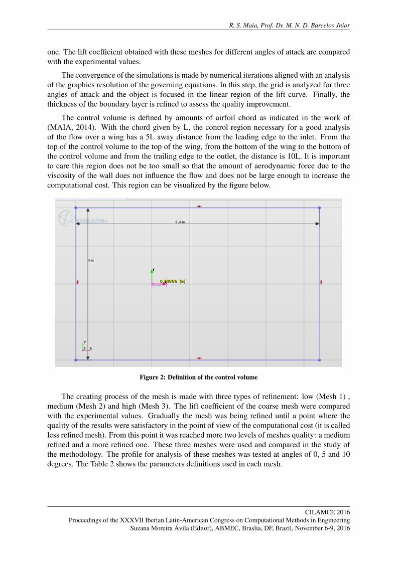
The control volume is defined by amounts of airfoil chord as indicated in the work of(MAIA, 2014). With the chord given by L, the control region necessary for a good analysisof the flow over a wing has a 5L away distance from the leading edge to the inlet. From thetop of the control volume to the top of the wing, from the bottom of the wing to the bottom ofthe control volume and from the trailing edge to the outlet, the distance is 10L. It is importantto care this region does not be too small so that the amount of aerodynamic force due to theviscosity of the wall does not influence the flow and does not be large enough to increase thecomputational cost. This region can be visualized by the figure below.

Figure 2: Definition of the control volume

The creating process of the mesh is made with three types of refinement: low (Mesh 1) ,medium (Mesh 2) and high (Mesh 3). The lift coefficient of the coarse mesh were comparedwith the experimental values. Gradually the mesh was being refined until a point where thequality of the results were satisfactory in the point of view of the computational cost (it is calledless refined mesh). From this point it was reached more two levels of meshes quality: a mediumrefined and a more refined one. These three meshes were used and compared in the study ofthe methodology. The profile for analysis of these meshes was tested at angles of 0, 5 and 10degrees. The Table 2 shows the parameters definitions used in each mesh.




Table 2: Parameters used for the mesh refinement.

Parameters Mesh 1 Mesh 2 Mesh 3

Base size 100 mm 100 mm 100 mm

Target surface size 5% 2.5% 2.5%

Minimum surface size 1% 0.1% 0.01%

Number of prism layers 4 4 4

Prism layer stretching 1.3 1.3 1.3

Prism layer total thickness 5% 5% 5%

Volume growth rate Fast Medium Slow

Maximum cell size 50mm 50mm 50mm

The base size parameter is a control variable as other parameters are defined as a percentageof it. In this experiment, it was defined as 100 mm, once the chord is 300 mm.

It can be noted by the Table 2 the mesh 3 is denser than mesh 2, and these, in turn, is denserthan mesh 1. This is justified by the quantity of elements from one to another.

The program calculates the elements size until the target surface size, however does notdiscard zones that need more refinement. In these zones, the elements which size is lower thanthe minimum surface size value are discarded.

The number of prism layers parameter indicates the quantity of elements layers present inthe boundary layer. This parameter was set to 4 elements. A total thickness of these layers isdefined by the parameter prism layer total thickness.

The thickness of each layer is determined by the previous layer with the prism layer stretch-ing parameter. In this problem, the thickness is set to 1.3 times the previous layer.

The volume growth rate parameter indicates the generation rate of the mesh size from onelayer to another. A fast growth rate, increase cell size quickly. On the other hand, a lower rate,indicates that the cell uses multiple mesh layers providing a gradual transition. This parametercan be better understood by the following figure.

Figure 3: Growth rate.

3.2 Turbulence model

In this section, the profile is analyzed to angles of attack of 0, 5, 10, 12, 15 and 18 degrees,with the k-epsilon, k-omega and Spalart-Allmaras turbulence models. The lift coefficients are




compared with the experimental values. It is important to remember that the experimentalvalues of work done by (WILLIAMSON et al., 2012) and (SELIG; GUGLIELMO., 1997) wereconducted in a controlled environment with the aid of a wind tunnel and hence the reliability ofthese results.

The mesh used for each angle of attack is the same, changing only the x, y and z compo-nents to obtain the flow angle recquired.

The turbulence model is defined according to the problem. For simulations involving flowover an airfoil, the RANS models meet satisfactorily the problem requirements and provideaccurate values for the resolution of the governing equations (CD-ADAPCO, 2015).

For the flow problem on the formula SAE vehicle wing, a steaty state was adopted. Thus,as the fluid is air and the compressibility effects are negligible, the equations are solved for idealgas due to this have good solution when it comes to determining the lift coefficient.

The solution of segregated flow solves the flow equations in a separated way and then themoviment and moment equations are connected by a corrective approximation. There are threetypes of segregated fluid energy used in StarCCM+. The temperature one is used in this paper.

The turbulence models adopted was the realizable k-epsilon with two layers; k-omega SST(Menter); and Spalart-Allmaras standard model.

In the first model, the transport equations are solved to the turbulent kinetic energy k andits dissipation psilon. It is able to deal with general flow and not only external ones (AIGUA-BELLA MACAU, 2011). The two layer model is a type of K-epsilon which uses low reynoldsnumber to apply K-epsion in the sublayers.

The K-omega SST (Shear Stress Transport) uses the especific dissipation rate instead of thedissipation used in K-epsilon. It solve the problem of applying the standard model to practicalproblems and it is sensible to the refinement of the mesh.

The last model solves a single transport equation to determine the turbulent viscosity. Thismethod is indicated for problems with associated boundary layer and flow with smooth detach-ment as a flow on airfoils.

4 RESULTS ANALYSIS

4.1 Mesh Convergence

The following figures show the level of convergence of each mesh for zero degrees of angleof attack. In order to assure the mesh of 2D is the same as 3D, the meshes were generated firstlyin 3D and with then converted to 2D by the command ”convert to 2D”.

Table 3: Number of elements of each mesh.

Mesh 1 Mesh 2 Mesh 3

Elements 2.183.143 9.849.521 9.850.255

This table indicates the number of elements generated for each mesh. The larger it is, themore refined will be the mesh.




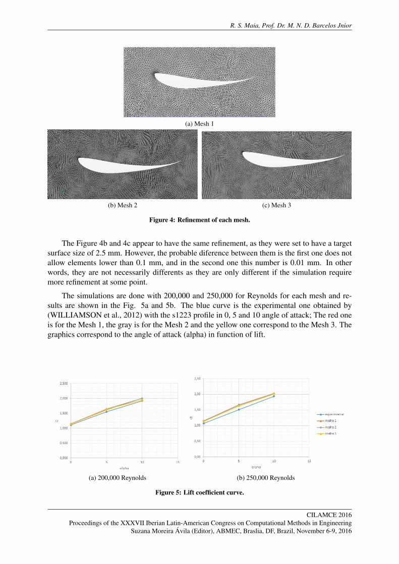
(a) Mesh 1

(b) Mesh 2 (c) Mesh 3

Figure 4: Refinement of each mesh.

The Figure 4b and 4c appear to have the same refinement, as they were set to have a targetsurface size of 2.5 mm. However, the probable diference between them is the first one does notallow elements lower than 0.1 mm, and in the second one this number is 0.01 mm. In otherwords, they are not necessarily differents as they are only different if the simulation requiremore refinement at some point.

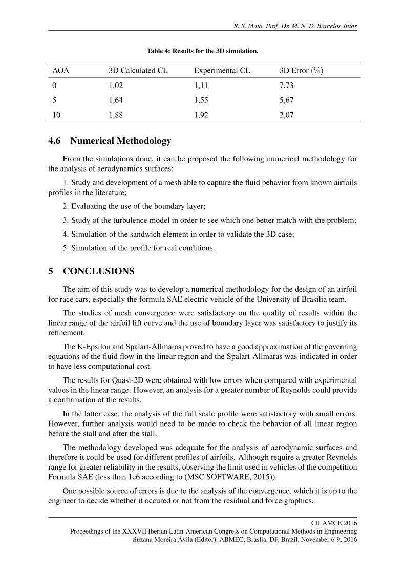
The simulations are done with 200,000 and 250,000 for Reynolds for each mesh and re-sults are shown in the Fig. 5a and 5b. The blue curve is the experimental one obtained by(WILLIAMSON et al., 2012) with the s1223 profile in 0, 5 and 10 angle of attack; The red oneis for the Mesh 1, the gray is for the Mesh 2 and the yellow one correspond to the Mesh 3. Thegraphics correspond to the angle of attack (alpha) in function of lift.

(a) 200,000 Reynolds (b) 250,000 Reynolds

Figure 5: Lift coefficient curve.




The Figures 5a and 5b show the lift curve in the linear region for the three meshes afore-mentioned. It is importante that the airfoil works inside this zone in order to avoid lift losscaused by stall.

The convergence study shows that the results are very close for the different meshes andfor the experimental curve. Analysing both graphics for 200,000 and 250,000 Reynolds, it ispossible to see that the use of more refined meshes does not improve the results.

4.2 Convergence of turbulence model

In the study of the convergence models, it is also used the two values of Reynolds, however,more angles of attack is simulated in order to know the behavior of each model throughout allthe linear curve.

The Spalart-Allmaras model uses one equation while the k-epsilon and k-omega use twoequations for the description of the fluid flow.

The Figure 6 represents the results for the simulation with 200,000 Reynolds of the differentturbulence models.

Figure 6: Lift curve of 200,000 Reynolds for different turbulence models.

For the Figure 6, it is possible to see that as the angle of attack increase, the error alsoincreases in a significant way. In this region, the k-epsilon and k-omega models need morerefinement. This can be explained by the fact that the equations of fluid flow and the governingequations of fluid dynamics do not converge totally.

The mean errors for each model is calculate by the Eq. 4

Error (%) =

∑ni Errorin

(4)

In the above equation, the angles above 15 degrees are discarded as these values are out ofthe linear curve and so the fluid are stalled. Thus:

k-epsilon =4,23%




k-omega =9,63%

Spalart-Allmaras=7,17%

According to Figure 6 it is possible to conclude that k-epsilon and Spalart-Allmaras mod-els have better approximations when compared with k-omega. However, evaluating for thecomputational cost, the Spalart is better because it uses only one equation as aforementioned.

For the 250,000 Reynolds, the results of the errors are:

k-epsilon=5,25%

k-omega=8,57%

Spalart-Allmaras=10,53%

Despite the errors of k-epsilon show better results, these values are not too significantbetween the models and so the Spalart model is chosen for the following sections.

4.3 Boundary Layer

The small region next to the surface is important to the description of the turbulence flows.This is duo to the fact that the turbulence begins when the fluid is dettached from the surface.The Equation 5 refers to the thickness of the boundary layer for flat plates (ANDERSON, 2001).The calculations are done for Reynolds of 200,000 with Spalart model model.

δ =0.3747L

Re0.2=

0.3747 ∗ 0.3200.0000.2

= 9.786mm (5)

The boundary layer is tested with 10, 20 and 30 layers. The Figure 7 shows the improve-ment of the results with the use of boundary layer. The simulation with 10 layers in yellow hasthe less error and proved to be useful.

Figure 7: Curve of Lift coefficient for Spalart model with 200,000 of Reynolds




The boundary layer was studied and provided more accurate values in comparison with thecomputational results according to the Fig.7. The difference for further refinement of the bound-ary layer can be justified by the fact that the increase of layers results in numerical roundingerrors.

4.4 Quasi-2d

The quasi-2D is a model 3D with so small thickness that can be compared with 2D. Thisprofile is studied in order to validate the 3D case from the 2D. This model is also known assandwich and can be saw by Fig. 8. The thickness is set to be 20 mm.

Figure 8: Thickness of the simulated airfoil

The results for the quasi-2D profile is shown by the Fig.9. The curves are simulated for200,000 of Reynolds with Mesh 1.

Figure 9: Comparison between quasi-2D, 2D and experimental curves.

It can be seen by the Figure 9 that the quasi-2D model has a large error for 18 angle ofattack. This can be explained by the presence of gradient of adverse pressure such vortexstructures which are commum when it occurs the detachment of the boundary layer.




4.5 3D

The 3D simulation is represented by the Fig. 10.

Figure 10: 3D model of the profile in the control volume.

The results of the simulation for 3D are shown in Fig. 11. For this case, it is simulated onlythree angle of attacks due to the high computational cost.

Figure 11: 3D curve compared with the experimental one.

In the Table 4 it is possible to see the errors of the linear region for full scale model.




Table 4: Results for the 3D simulation.

AOA 3D Calculated CL Experimental CL 3D Error (%)

0 1,02 1,11 7,73

5 1,64 1,55 5,67

10 1,88 1,92 2,07

4.6 Numerical Methodology

From the simulations done, it can be proposed the following numerical methodology forthe analysis of aerodynamics surfaces:

1. Study and development of a mesh able to capture the fluid behavior from known airfoilsprofiles in the literature;

2. Evaluating the use of the boundary layer;

3. Study of the turbulence model in order to see which one better match with the problem;

4. Simulation of the sandwich element in order to validate the 3D case;

5. Simulation of the profile for real conditions.

5 CONCLUSIONS

The aim of this study was to develop a numerical methodology for the design of an airfoilfor race cars, especially the formula SAE electric vehicle of the University of Brasilia team.

The studies of mesh convergence were satisfactory on the quality of results within thelinear range of the airfoil lift curve and the use of boundary layer was satisfactory to justify itsrefinement.

The K-Epsilon and Spalart-Allmaras proved to have a good approximation of the governingequations of the fluid flow in the linear region and the Spalart-Allmaras was indicated in orderto have less computational cost.

The results for Quasi-2D were obtained with low errors when compared with experimentalvalues in the linear range. However, an analysis for a greater number of Reynolds could providea confirmation of the results.

In the latter case, the analysis of the full scale profile were satisfactory with small errors.However, further analysis would need to be made to check the behavior of all linear regionbefore the stall and after the stall.

The methodology developed was adequate for the analysis of aerodynamic surfaces andtherefore it could be used for different profiles of airfoils. Although require a greater Reynoldsrange for greater reliability in the results, observing the limit used in vehicles of the competitionFormula SAE (less than 1e6 according to (MSC SOFTWARE, 2015)).

One possible source of errors is due to the analysis of the convergence, which it is up to theengineer to decide whether it occured or not from the residual and force graphics.




REFERENCES

AIGUABELLA MACAU, R. Formula one rear wing optimization. master thesis. UniversitatPolitecnica de Catalunya, 2011.

AIRFOILTOOLS. Airfoil plotter. s1223-il.acesso em 21 de maio de 2015. 2015. Disponıvel em:〈Airfoiltools.com〉.

ANDERSON, J. Fundamentals of aerodynamics. Traducao. [S.l.: s.n.], 2001.

CD-ADAPCO. Steve portal. documentation. 2015. Acesso em: 5 maio 2015. Disponıvel em:〈https://steve.cd-adapco.com/Home〉.

EQUIPE ICARUS. Poli ufrj. 2015. Disponıvel em: 〈http://www.equipeicarus.poli.ufrj.br/?page=competicao〉.

FORMULA 1. Inside f1. understanding f1 racing. aerodynamics. acessado em 3 de maio de2015. 2015. Disponıvel em: 〈http://www.formula1.com/content/fom-website/en/championship/inside-f1/understanding-f1-racing/aerodynamics.html〉.

KATZ, J. Racecar aerodynamics. [S.l.: s.n.], 1995.

KIEFFER, W.; MOUJAES, S.; ARMBYA, N. Cfd study of section characteristics of formulamazda race car wings. mathematical and computer modelling. p. 1275–1287.

MAIA, R. S. Cfd analysis concept, school of engineering and technology. University of derby,2014.

MSC SOFTWARE. Academic case studies, cal poly pomona formula sae team. n.p., 2015. web.2015.

PAKKAM, S. High downforce aerodynamics for motorsports. [raleigh, north carolina]. NorthCarolina State University., 2011.

SELIG, M. S.; GUGLIELMO., J. J. ’high-lift low reynolds number airfoil design’. journal ofaircraft 34.1. p. 72–79. Web., 1997.

WILLIAMSON, G. A. et al. Summary of low speed airfoil data, vol 5. University of Illinois,Department of Aerospace Engineering, Urbana-Champaign, 2012.



development of a numerical methodology for the …

Documents