Development of a SensorPlatform for Roadway Mapping:

Part B – Mapping the RoadFog Lines

Max Donath, Principal Investigator Intelligent Vehicles Laboratory

Department of Mechanical Engineering University of Minnesota

April 2015

Research ProjectFinal Report 2015-11

To request this document in an alternative format call 651-366-4718 or 1-800-657-3774 (Greater Minnesota) or email your request to ADArequest.dot@state.mn.us. Please request at least one week in advance.

Technical Report Documentation Page 1. Report No. 2. 3. Recipients Accession No. MN/RC 2015-11 4. Title and Subtitle Development of a Sensor Platform for Roadway Mapping: Part B – Mapping the Road Fog Lines

5. Report Date April 2015 6.

7. Author(s) 8. Performing Organization Report No. Brian Davis, Max Donath 9. Performing Organization Name and Address 10. Project/Task/Work Unit No. Department of Mechanical Engineering University of Minnesota 111 Church Street SE Minneapolis, MN 55455

CTS Project #2014019 11. Contract (C) or Grant (G) No.

(c) 99008 (wo) 115

12. Sponsoring Organization Name and Address 13. Type of Report and Period Covered MN Local Road Research Board Minnesota Department of Transportation Research Services & Library 395 John Ireland Boulevard, MS 330 St. Paul, Minnesota 55155-1899

Final Report 14. Sponsoring Agency Code

15. Supplementary Notes http://www.lrrb.org/pdf/201511.pdf 16. Abstract (Limit: 250 words) Our objective is the development and evaluation of a low-cost, vehicle-mounted sensor suite capable of generating map data with lane and road boundary information accurate to the 10 cm (4 in) level. Such a map could be used for a number of different applications including GNSS/GPS based lane departure avoidance systems, smart phone based dynamic curve speed warning systems, basemap improvements, among others.

The sensor suite used consists of a high accuracy GNSS receiver, a side-facing video camera, and a computer. Including cabling and mounting hardware, the equipment costs were roughly $30,000. Here, the side-facing camera is used to record video of the ground adjacent to the passenger side of the vehicle. The video is processed using a computer vision algorithm that locates the fog line within the video frame. Using vehicle position data (provided by GNSS) and previously collected video calibration data, the fog line is located in real-world coordinates.

The system was tested on two roads (primarily two-lane, undivided highway) for which high accuracy (<10 cm) maps were available. This offset between the reference data and the computed fog line position was generally better than 7.5 cm (3 in).

The results of this work demonstrate that it is feasible to use a camera to detect the position of a road’s fog lines, or more broadly any other lane markings, which when integrated into a larger mobile data collection system, can provide accurate lane and road boundary information about road geometry.

17. Document Analysis/Descriptors 18. Availability Statement Mobile computing, Global Positioning System, Satellite navigation systems, Computer vision, Rural areas, Driver support systems, Vehicle safety, Ran off road crashes, lane departure warning systems.

No restrictions. Document available from: National Technical Information Services, Alexandria, Virginia 22312

19. Security Class (this report) 20. Security Class (this page) 21. No. of Pages 22. Price Unclassified Unclassified 44

Development of a Sensor Platform for

Roadway Mapping: Part B – Mapping the Road Fog Lines

Final Report

Prepared by:

Brian Davis Max Donath

Intelligent Vehicles Laboratory

Department of Mechanical Engineering University of Minnesota

April 2015

Published by: Minnesota Department of Transportation

Research Services & Library 395 John Ireland Boulevard, MS 330

St. Paul, Minnesota 55155-1899 This report represents the results of research conducted by the authors and does not necessarily reflect the official views or policies of the Local Road Research Board (LRRB), the University of Minnesota, or the Minnesota Department of Transportation. This report does not contain a standard or specified technique. The authors, the Local Road Research Board (LRRB), the Minnesota Department of Transportation, and the University of Minnesota do not endorse products or manufacturers. Any trade or manufacturers’ names that may appear herein do so solely because they are considered essential to this report.

Acknowledgments This project was funded by the Local Road Research Board (LRRB) and the University of Minnesota’s Center for Transportation Studies and the Intelligent Transportation Systems Institute. The authors would like to thank the following individuals for their generous help and support with this project:

• Rick West (who led our Technical Advisory Panel) and Chuck Grotte of Otter Tail County

• Joe Gustafson (who reviewed the report and provided feedback), David Brandt and Charlie Parent of Washington County

• Derek Leuer of MnDOT, for his assistance with identifying high-priority crash-risk road segments in the counties

• Peter Jenkins of MnDOT for his assistance with obtaining data provided by Continental Mapping and reviewing the report

• Brad Canaday, Trisha Stefanski, Peter Morey, and Brad Estochen of MnDOT for their assistance reviewing the report and providing insightful comments throughout the project

• Rodney Dockter for his assistance with the software

Table of Contents

1 Introduction ............................................................................................................................. 1

1.1 Lane departure in rural areas ............................................................................................ 1

1.2 Objective .......................................................................................................................... 1

1.3 Project Scope .................................................................................................................... 2

2 Proposed System...................................................................................................................... 4

2.1 Hardware .......................................................................................................................... 4

2.1.1 GNSS ........................................................................................................................ 4

2.1.2 Camera ...................................................................................................................... 5

2.1.3 Computer................................................................................................................... 7

2.1.4 Mounting Equipment ................................................................................................ 7

2.2 Post-Processing Software ................................................................................................. 9

3 System Evaluation Methods .................................................................................................. 12

3.1 Data Collection and Analysis ......................................................................................... 12

3.2 Test Areas ....................................................................................................................... 12

3.2.1 United States Highway 63 ...................................................................................... 13

3.2.2 Minnesota State Highway 23 .................................................................................. 14

3.3 Reference Data ............................................................................................................... 15

4 Results ................................................................................................................................... 16

4.1 US 63 .............................................................................................................................. 16

4.2 MN 23 ............................................................................................................................ 23

5 Discussion and Conclusions .................................................................................................. 30

5.1 Fog Line Detection and Positioning ............................................................................... 30

5.2 Sources of Residual Error and Anomalies ..................................................................... 30

5.2.1 Sensor Error ............................................................................................................ 30

5.2.2 Timing Ambiguity and Synchronization ................................................................ 30

5.2.3 Lane Marking Visibility and Quality ...................................................................... 30

5.2.4 Error vs Offset......................................................................................................... 31

5.2.5 Lane Re-striping...................................................................................................... 31

5.3 Future Work ................................................................................................................... 31

5.4 Final Conclusions ........................................................................................................... 32

6 References ............................................................................................................................. 33

List of Figures

Figure 2.1: Minnesota CORS/RTRN GNSS network as of March 11, 2014 (from: [7]) ............... 4 Figure 2.2: Trimble BX982 receiver and Zephyr-2 antenna (from: [8,9]) ..................................... 5 Figure 2.3: Sample frame collected from camera ........................................................................... 6 Figure 2.4: iDS UI-3250CP camera and Kowa LMVZ4411 lens (from: [10, 11]) ........................ 6 Figure 2.5: Vehicle mounts and sensor pod on Chevrolet Impala .................................................. 8 Figure 2.6: Vehicle mounts and sensor pod on Metro District’s video logging van ...................... 9 Figure 2.7: Region of interest within full image frame ................................................................ 10 Figure 3.1: US 63 test area data extent ......................................................................................... 13 Figure 3.2: MN 23 test area data extent (basemap from ESRI) .................................................... 14 Figure 4.1: US 63 data extent with figure locations ..................................................................... 17 Figure 4.2: US 63 – Location A .................................................................................................... 18 Figure 4.3: US 63 – Magnified view of location A ...................................................................... 18 Figure 4.4: US 63 – Location B .................................................................................................... 19 Figure 4.5: US 63 – Magnified view of location B....................................................................... 19 Figure 4.6: US 63 – Location C .................................................................................................... 20 Figure 4.7: US 63 – Location D .................................................................................................... 21 Figure 4.8: US 63 – Location E .................................................................................................... 22 Figure 4.9: US 63 – Location F .................................................................................................... 23 Figure 4.10: MN 23 data extent with figure locations .................................................................. 24 Figure 4.11: MN 23 – Location A ................................................................................................ 25 Figure 4.12: MN 23 – Magnified view of location A ................................................................... 26 Figure 4.13: MN 23 – Close up view of location A...................................................................... 26 Figure 4.14: MN 23 – Location B ................................................................................................. 27 Figure 4.15: MN 23 – Location C ................................................................................................. 28 Figure 4.16: MN 23 – Magnified view of location C ................................................................... 29 Figure 5.1: Example of poor quality fog line ................................................................................ 31

List of Tables

Table 4.1: Fog Line Offset Analysis for US 63 ............................................................................ 16 Table 4.2: Fog Line Data for MN 23 ............................................................................................ 23

Executive Summary Roadway departure crashes represent a major road-safety issue on both the national and state level. Infrastructure-based countermeasures including pavement treatments (e.g., rumble strips) have had success, but not enough to significantly reduce the large fraction of road fatalities that run-off-road (ROR) crashes represent. Newer, more accurate, Global Navigation Satellite Systems (GNSS) technologies open up many possibilities, in particular, the potential of in-vehicle GNSS-based lane departure warning systems (LDWS) especially for wintery climates where lane markings are inadequate to trigger vision-based LDWS. However, these new driver assist systems would require high accuracy maps that represent the road and its boundaries. Our objective is the development and evaluation of a low-cost, vehicle-mounted sensor suite capable of generating map data with lane and road boundary information accurate to the 10 cm (4 in) level. An inexpensive method for acquiring a state-wide map of such accuracy would have many applications besides LDWS and would especially benefit rural counties, which do not typically have access to high-end systems. For example, more accurate measures of road curvature acquired inexpensively and automatically could be used to better match speed limits with curves and provide curve-speed warnings using smartphones, especially where low average daily traffic volumes (ADTs) do not justify signage on a system-wide basis. In the first phase of the project, and as detailed in the report Development of a Sensor Platform for Roadway Mapping: Part A - Road Centerline and Asset Management [1], a data collection platform was developed that consisted of a GNSS receiver capable of receiving real-time corrections, a LIDAR (light detection and ranging) scanner and a computer, which along with mounting hardware, was purchased for roughly $40,000. It was shown that using this hardware, the system could detect and position curbs and guardrails with an accuracy of better than 10 cm. Additionally, the system could determine road centerlines to within 6 cm (2 in) in areas where applicable without the use of the LIDAR, relying only on GNSS-provided vehicle-path information. There were limitations; however, these are outlined in the first phase report. This report details the second phase of a project that seeks to extend the work done in the first phase by augmenting the system with a video camera for automated fog line detection and positioning. This report focuses on this effort and the evaluation thereof. Video data is captured by a side-facing camera that views an area of the ground adjacent to the passenger side of the vehicle. The video is collected and stored for later processing to extract the position of the fog line by applying a computer vision algorithm that locates the fog line within the video frame under a variety of lighting conditions. The position of the line in the frame is converted to a distance from the vehicle based on calibration information. The line’s distance from the vehicle is then used to determine the fog line’s position in world coordinates by using the vehicle’s position information obtained through the GNSS receiver. The system was tested on two roads for which high accuracy (<10 cm) maps were available. Both were roads that were primarily two-lane, undivided highway, a configuration common among rural roads where lane departure crashes are common. The results compared the offset between the fog line position determined by our system with the fog line position in the reference

data. This offset was generally better than 7.5 cm (3 in), which is within our design goal of achieving an accuracy of 10 cm. LIDAR was not needed for determining fog line positions, thus reducing the cost of the sensor suite to $30,000 for this application. Future potential improvements include additional automation of the process, adding cameras to acquire more information about the roadway (e.g. centerline striping, road signs), and continued development to extract additional types of road information. The results of this work demonstrate that it is feasible to use a camera to detect the position of a road’s fog lines, or more broadly any other lane markings, which when integrated into a larger mobile data collection system, can provide accurate lane and road boundary information about road geometry.

1

1 Introduction Roadway departure crashes represent a major road safety issue on both the national and state level. Infrastructure-based countermeasures including pavement treatments (e.g., rumble strips) have had success, but not enough to significantly reduce the large fraction of road fatalities that Run-Off-Road (ROR) crashes represent.. Newer, higher accuracy Global Navigation Satellite Systems1 (GNSS) technologies open up many possibilities, in particular, the potential of in-vehicle GNSS-based lane departure warning systems (LDWS) especially for wintery climates where lane markings are inadequate to trigger vision-based LDWS. However, these new driver assist systems would require high accuracy maps that represent the road and its boundaries. 1.1 Lane departure in rural areas A recent report by CH2M Hill [2] discusses the process of creating county safety plans in the state of Minnesota including their system-wide crash analysis and risk assessment. They found that throughout Minnesota, about 80% of serious crashes, those involving a serious injury or fatality, occurred on state and county roads with the other 20% occurring on city, township and other roads. Additionally, of crashes on county systems, 83% were in rural areas. Of these rural crashes, about half of them are caused by lane departures. Because of this, the report lists run-off-road crashes among crash types representing the greatest opportunity for reduction. This is further supported by 2012 data published by the Minnesota Department of Public Safety stating that 51% of fatal crashes were due to vehicles leaving their lane [3]. The CH2M Hill report also indicates that low volume roads comprise a substantial number of Minnesota’s severe run-off-road crashes. 65% of severe run-off-road crashes on Minnesota’s county roads occur on roadways with less than 1000 vehicles per day. Another risk factor identified was the frequency and radius of curvature of horizontal curves. Curve radii between 500 and 1200 feet presented the highest risk factor accounting for approximately 50% of curves along county roadways and 63% of severe crashes. 1.2 Objective The CH2M Hill report shows that lane departures in rural areas represent a significant portion of severe and fatal crashes in Minnesota. One way to begin to reduce these types of crashes is through the use of GNSS-based, in-vehicle lane departure warning systems. These systems use high accuracy differential GNSS to determine the real-time position of the vehicle and digital maps containing lane boundary information to determine where the vehicle is in relation to the lane boundaries. With advance knowledge of the location of high-risk curves or other hazards provided by a map, the system can then warn the driver before they begin to leave their lane, even under conditions where real time sensing of the lane boundaries would be difficult (i.e. snow, heavy rain, etc.). We believe that higher accuracy GNSS not requiring differential corrections will likely be available within 5 years when the full constellation of newer GNSS satellites is in orbit.

1 In this report, the term Global Navigation Satellite System (GNSS) is used instead of Global Positioning System (GPS) for consistency with the literature and to reflect the fact that many GNSS receivers (including the one used in this project) receive signals from multiple Global Navigation Satellite Systems (i.e. GPS, GLONASS, Galileo, Compass, etc.).

2

Our objective is the development and evaluation of a low-cost (under $40k) vehicle-mounted sensor suite capable of generating map data with lane and road boundary information accurate to the 10 cm (4 inch) level. An inexpensive method for acquiring a state-wide map of such accuracy would have many applications besides LDWS and would especially benefit rural counties which do not typically have access to high-end systems. For example, more accurate measures of road curvature acquired inexpensively and automatically could be used to better match speed limits with curves and provide curve-speed warnings using smartphones, especially where low ADT’s do not justify signage on a system wide basis. Work on automated detection and characterization of road curvature data has been performed at the University of Wisconsin [4] and Iowa State University [5]. Their work describes automated methods by which road curvature data could be extracted from existing map data or collected GNSS data. This data would be useful for a number of applications on rural roads. We believe that smartphone-based Assisted-GPS (A-GPS) systems have improved significantly and it is possible to develop and deploy dynamic curve speed warning systems deployed as a smartphone app that capture the attention of drivers before they run off the road at high risk curves. The efficacy of such systems obviously relies on the availability and quality of high accuracy map data. The focus of this project is the generation of these maps. In addition to lane departure warning systems, the high accuracy map data as well as the raw collected data such as vehicle path, LIDAR (light detection and ranging) scans, and video can also be used for a number of other applications including GIS basemap creation and maintenance, inventory tracking, pavement monitoring, lane marking maintenance, etc. The key is to design a system that is capable of collecting data suitable for as many applications as possible while still maintaining fiscal efficiency. The system designed in this project seeks first to create high accuracy maps while leaving open the option to use the collected data in other ways. 1.3 Project Scope This research seeks to extend the work performed in Part 1 of this project. Part 1 focused on the creation of a system capable of locating guard rails and curbs through the use of a relatively inexpensive, commercially available LIDAR scanner paired with GNSS. The report for Part 1 [1] discusses the system as well as provides additional context including a summary of the state of mobile data collection (including mobile LIDAR). It also elaborates on the state of lane departure avoidance systems and the motivation for using a GNSS based system over the more common vision-based systems. The experiments performed in Part 1 seek to determine the accuracy with which the developed system can detect guard rails, curbs and calculate centerlines in urban and rural environments. One overlapping focus of both parts is the evaluation of methods to determine a high accuracy road centerline data for roads with simple or well understood geometries. The result of this analysis is presented in the report for Part 1 [1] which discusses the hardware (section 2.1), software (section 2.2.1), the test area where the data was collected (section 3.2.2), the results (section 4.1) and a discussion of the results (5.1). This analysis showed that the methods utilized could calculate the position of the road centerline to an accuracy of around 6 cm for roads with simple or well understood geometries such as two lane, undivided highways. These results were within the 10 cm accuracy goal.

3

The work performed in Part 2 extends the prior work by augmenting the data collection system’s capabilities with the addition of a side-looking video camera which can provide additional information about lane boundaries. Specifically, this report will focus on the system used to collect video data, analyze it, and create maps of roadway fog lines. The resulting fog line data will be compared to available high accuracy reference data for two test areas, a segment of US 63 near Red Wing, MN and a segment of MN 23 south of Granite Falls, MN. Additionally, county system roads were also driven in Otter Tail and Washington counties. High risk roads were selected to be mapped based on their county safety plan risk assessment. However, because no high accuracy reference map data is available for these areas, these results are not included in this report but will be delivered in the form of shapefiles to those counties. Please note that the data for the roads driven in these two counties should exhibit the same accuracy as achieved for the test areas discussed in this report.

4

2 Proposed System The focus of the system developed in this project is to generate high accuracy road fog line position data for use in basemaps, lane departure warning systems, and other applications. The goal is to capture these road features accurate to 10 cm using a system whose components cost roughly $30,000. This accuracy level is considered to be a good tradeoff between being accurate enough to be used in a number of applications while still being cost effective to collect on a wide scale. This section describes the hardware used to accomplish this as well as the algorithms needed to process the raw data to generate useful information. 2.1 Hardware 2.1.1 GNSS The positioning system used in this project is a single GNSS receiver capable of determining a real time kinematic (RTK) solution. RTK is a method by which a GNSS receiver calculates a highly accurate, real time position solution by combining carrier phase measurements with corrections information from base stations. Here, the corrections are provided by MnDOT’s statewide Continuously Operating Reference Station/Real-Time Reference Network (CORS/RTRN) GNSS. The corrections are accessed over the internet using a wireless modem with a cellular data plan. Many states and other private groups operate CORS networks including those using the same Trimble Virtual Reference Station (VRS) software that MnDOT operates [6]. A map of the Minnesota system is shown in Figure 2.1.

Figure 2.1: Minnesota CORS/RTRN GNSS network as of March 11, 2014 (from: [7])

5

The receiver combines the raw position information obtained through its antenna with the real-time corrections data available over the internet to calculate its position. The resulting position information is obtained from the GNSS receiver and interpolated for camera frames collected between position fixes. The GNSS receiver used in this project is the Trimble BX982 which is paired with a single Trimble Zephyr Antenna. The receiver and antenna used are shown (not to scale) in Figure 2.2.

Figure 2.2: Trimble BX982 receiver and Zephyr-2 antenna (from: [8,9])

The Trimble BX982 is a receiver capable of calculating position fixes with a stated horizontal accuracy of 8 mm + 1 part per million (ppm calculated with respect to the distance to the nearest correction station) RMS. The receiver is set to provide these fixes 10 times per second. For a data collection vehicle moving at 55 mph, this corresponds to a position update every 2.5 meters. This receiver is commercially available and costs about $16,000. 2.1.2 Camera The camera allows the system to detect and locate the position of the fog line with respect to the vehicle. For this application, it is mounted inside an enclosure on the right (passenger) side of the vehicle and faces downward so that its field of view contains the pavement adjacent to the vehicle to about 3 meters away from the side of the vehicle. A representative sample image taken from the camera is shown in Figure 2.3: Sample frame collected from camera to illustrate the camera’s field of view.

6

Figure 2.3: Sample frame collected from camera This image shows the white fog line on the gray pavement. Beyond the pavement, the gravel shoulder is visible. The camera housing and LIDAR bug screen occludes a portion of the image frame and is visible in the top right and bottom right corners of the image, respectively. The red number in the top left of the image is the timestamp when the frame was captured. The camera used in this project is the iDS UI-3250CP which was paired with the Kowa LMVZ4411 lens which are shown in Figure 2.4.

Figure 2.4: iDS UI-3250CP camera and Kowa LMVZ4411 lens (from: [10, 11])

7

Additionally, a polarizing filter was used to mitigate glare in the lens caused by the sun. The camera is configured to collect video at 30 frames per second at a resolution of 1600 by 1200 pixels. When traveling at 55 mph, this corresponds to a frame captured every 0.82 meters. The camera and lens were purchased for a combined cost of approximately $1300. 2.1.3 Computer A computer is required to communicate with the sensors in order to initialize them and acquire the data. In our case, the computer used was a consumer laptop that costs around $2000. It must be fast enough to run the sensor drivers and collect the data, but because no post-processing or analysis is performed in real time, it can have moderate specifications. Although the computer does not affect the accuracy of the system in any way, it is included in this discussion because it performs a critical function without which the system could not function. 2.1.4 Mounting Equipment It is important that the equipment be attached securely to the data collection vehicle. The method utilized here is a two-part solution consisting of the vehicle mounts and the sensor pod. The vehicle mounts connect to the vehicle and provide a connection point for the sensor pod. The bars are mounted so that they are parallel to each other and the ground and perpendicular to the car’s direction of travel. Once the vehicle mounts are installed, the sensor pod attaches easily by sliding on the ends of the bars and clamping in place with set screws. The advantage of using a system like this is that the vehicle mounts can be left on the vehicle even when the sensor pod is removed. The sensor pod itself is adjustable so that the orientation of the sensors can be changed allowing for flexibility throughout this and future projects. Because the camera can be repositioned, it must be re-calibrated every time it is moved. This is performed by collecting images with a marker or scale placed at known distances away from the vehicle. This allows for a function to be created that maps the relationship between the pixel location of an object in the image to its real world position with respect to the vehicle.

8

For the primary research vehicle, a Chevrolet Impala, the mounts are a commercially available off the shelf roof rack that consist of two aluminum bars attached to the top of the vehicle with clamps that attach to the door frames. The vehicle mounts and sensor pod are shown attached to the Chevrolet Impala in Figure 2.5.

Figure 2.5: Vehicle mounts and sensor pod on Chevrolet Impala

Custom vehicle mounts were also fabricated to allow for the system to be installed on a MnDOT pavement monitoring van. This type of van was selected because these vehicles drive the roads for other purposes, thus serving as a data collection platform that could be used with this system for a small incremental cost. Here, vehicle mounts were constructed that clamped on to the rain gutter of the van which then support aluminum bars similar to those used on the Chevrolet Impala. This provides the same connection point for the sensor pod allowing for the same sensor pod to be used on either vehicle. The vehicle mounts for the van along with the sensor pod in this configuration are shown in Figure 2.6.

9

Figure 2.6: Vehicle mounts and sensor pod on Metro District’s video logging van

2.2 Post-Processing Software Extracting road features such as lane markings can be resource intensive depending on the methods used to collect and process the raw data. The goal of this project was to design data processing software that would require as little human intervention as possible and yet, accommodate different ambient lighting and pavement conditions. For the purposes of detecting the position of the fog line, a computer vision algorithm was developed to determine the position of the fog line from the collected video. Using this algorithm allows for an automated post-processing workflow not requiring human intervention to identify the location of the fog line. Work in the field of video-based lane marking detection generally focus on forward facing cameras. Using such a camera configuration allows for more data to be collected about the vehicle’s current surroundings [12,13,14]. Specifically, the forward looking imaging systems allow both lane markings to be detected at once with the same camera which enables calculations to determine the vehicle’s lane position. However, the tradeoff is that the software required to do this is more complex. The software developed for our project focused on a straight forward algorithm that can be implemented and evaluated within the project timeline. The goal of the video analysis algorithm is to use the collected videos and the GNSS provided vehicle position data to determine the location of the fog line for a driven road. This is accomplished by first identifying the location of the fog line within an image, then converting the line’s position within the frame to its position with respect to the vehicle, and finally combining that with the vehicle position data to determine the line’s position in world coordinates.

10

The fog line is located through the use of a computer vision algorithm which detects the presence and location of a paint stripe within the image by searching for a horizontal band whose pixels have higher brightness values than the pixels outside that band. First the raw image from the camera is cropped to reduce the amount of processing required to determine the position of the line. The crop was selected to balance processing time by only including areas where the fog line is most frequently located within the frame. The region of interest is a 1300 by 600 pixel subset located in the bottom left hand of the original image. Figure 2.7 illustrates the size and location of the region of interest.

Figure 2.7: Region of interest within full image frame

Next, the image is transformed from color to grayscale. This is done because searching for a white line on darker pavement doesn’t require the information provided by color. Then a series of binary thresholds are independently applied to the image. A binary threshold is a process that considers the brightness of each pixel and determines whether or not it meets the given threshold value. If it is darker than that value, the pixel is set to black and if it’s higher than that value, the pixel is set to white. The resulting image is binary black and white (i.e. every pixel is either black or white but never gray). This is performed for 20 different threshold values ranging from very dark to very light. The goal of this operation is to find a threshold for which the fog line is set to white and the adjacent

11

pavement is set to black. The reason so many values must be used is because it is not possible to predict the relative brightness of the image a priori. That is to say, even though the fog line appears lighter than the pavement, the absolute brightness values of both the fog line and the pavement change based on the ambient lighting conditions. For example, the overall image brightness can be affected by time of day, cloud cover, and shadows due to trees, buildings, and the vehicle itself. Next, the collection of thresholded images is analyzed to determine whether or not there is a horizontal band of white pixels surrounded by black pixels. This is done by summing the number of white pixels in each pixel row resulting in a 1-dimensional histogram where each bin represents a single pixel row. Then, the gradient, or derivative, of this histogram is calculated which represents the change in brightness of a given pixel row. With this information, it is then possible to determine whether a horizontal, white line exists in the image by determining if there is a gradient peak (representing dark to light) and then an accompanying valley (representing light to dark). This peak and valley represent the top and bottom of the fog line. If the distance between the top and the bottom of the line are consistent with a fog line, the algorithm then saves the position of the line as the midpoint between them. This process is performed on all 20 of the thresholded images which generally results in between 1 and 8 calculated lines each located with a different threshold value. The algorithm then calculates and reports the median position of all the lines located in that image which results in a single, final line position for the frame. To determine the position of the line with respect to the vehicle, the software uses a polynomial function generated during calibration. The calibration procedure begins by using the camera to take images of markers placed on the ground next to the vehicle at known distances from the vehicle. Then, the markers are located within the images (i.e. the row in which the marker appears is noted). This yields a set of pixel row, distance pairs that can be used to calculate a 3rd order polynomial fit relating pixel row locations within the image to a distance from the vehicle. This process takes care of the trigonometric relationship between the imaging sensor and the ground as well as any lens distortion. This process is only performed once each time the camera is moved. After determining the position of the fog line with respect to the vehicle using the function described above, the software then combines that with information about the vehicle’s location as provided by the GNSS. This yields the fog line’s position in real world coordinates. Because the software requires the vehicle’s position in real world coordinates to determine the location of the detected fog lines, the accuracy with which the fog lines are located is highly dependent on the quality of the GNSS receiver’s position fix. That is to say, if the GNSS does not have a high accuracy position fix, the system can’t provide a high accuracy line position. This procedure is performed for every frame in the video in order to generate a series of points that when combined, constitute the calculated position of the fog line.

12

3 System Evaluation Methods 3.1 Data Collection and Analysis Our evaluation seeks to determine the accuracy with which the system can determine the position of a road’s fog lines. This was conducted by first collecting video and GNSS data in two test areas and then processing the data to produce the fog line location information. The calculated fog lines can then be compared, where applicable, to reference data. Then, the offset between these two data sources can be calculated to determine the system’s accuracy.

For each test area, the road segment was driven multiple times in each direction. The path for each pass was the same, always taking the right most thru lane. Data for both test areas were collected in the fall of 2014. 3.2 Test Areas Data was collected for evaluation in two test areas chosen due to the availability of high accuracy map data that could be used as a reference against which the computed data can be evaluated. Originally, the goal was to use information obtained in the analysis of the county road safety plans to help inform the decision of where to test the system. However, this method presented issues because those roads identified in partner counties did not already have high accuracy map data to which system results could be compared.

13

3.2.1 United States Highway 63 The first test area is a 2.8 mile stretch of US 63 between US 61 in Red Wing, MN and Wisconsin State Highway 35 in Hagar City, WI. This road is an undivided two lane highway that includes two major bridges crossing the Mississippi River and Wisconsin Channel. The extent of this test area is shown in Figure 3.1 superimposed on orthorectified imagery from Wisconsin DOT.

Figure 3.1: US 63 test area data extent

14

3.2.2 Minnesota State Highway 23 The second test area is an 18.6 mile stretch of MN 23 between US 212 in Granite Falls, MN and Lyon County Road 73, approximately 3 miles south of Cottonwood, MN. Except for two relatively short portions, this road is a 2 lane, undivided highway. The extent of this test area is shown in Figure 3.2 superimposed on a basemap from ESRI and their data partners.

Figure 3.2: MN 23 test area data extent (basemap from ESRI)

15

3.3 Reference Data The reference data was provided by Continental Mapping, a contractor from Sun Prairie, Wisconsin. They drove the test areas with a Riegl VMX-250 mobile LIDAR scanning system in the summer of 2013 and then processed the resulting point cloud to extract lane and road boundary information. For US 63, the raw point cloud data has a specified horizontal accuracy of 5.39 cm or better and the extracted road features have a stated accuracy of 10 cm or better. For MN 23, the raw point cloud has a specified accuracy of 1.5 cm and no stated accuracy for the extracted features. The reference data contains, among other features, the locations of painted lane markings. These elements are each represented by a line string, which is a series of connected points. The reported position for the painted fog line markings is the center of the line which is consistent with the methods used in our system.

16

4 Results The results consist of a quantitative and qualitative analysis of the fog line detection and positioning. The quantitative analysis consists of the fog line detection and positioning evaluation for the two test areas. Our quantitative accuracy analysis calculates the mean and standard deviation of the offsets between the computed fog lines and the reference data for each pass. A pass consists of traveling once along the entire length of the test area in a single direction. The calculations were done by projecting or transforming both the calculated and reference data into the Minnesota South State Plane coordinate system [15]. The mean and standard deviation data is presented in meters. It’s important to note that these values do not give any information about whether the detected fog line was closer to or further from the vehicle than the reference data fog line. Passes are numbered based on the order in which they were driven and the direction of travel is designated with NB or SB for north and south bound passes respectively. In addition to the quantitative results, a number of sample results are presented showing the calculated position data represented by points superimposed on the reference data and orthorectified aerial photography which is used for context but not to determine a measure of accuracy. The imagery for locations within Minnesota was provided by MnDOT and has a pixel size (resolution) of 0.15 meters. Similarly, for locations in Wisconsin, the imagery was provided by the Wisconsin DOT and has a pixel size (resolution) of 0.30 meters. The results used in both the quantitative analysis and shown in the figures below contain the raw output of the post-processing. That is to say the results have not been “cleaned-up” or modified by human intervention. 4.1 US 63 Data was collected for US 63 in 4 passes (2 in each direction). The results of each pass are shown in Table 4.1 in the order in which they were collected. The last row is an aggregated total for all the passes.

Table 4.1: Fog Line Offset Analysis for US 63 Pass Name Number of

Samples Mean Error [m] Standard

Deviation [m] NB 1 4445 0.085 0.106 SB 1 4316 0.067 0.181 NB 2 4680 0.078 0.076 SB 2 4816 0.066 0.010 Total 19257 0.074 0.108

The results show that generally, the offsets between the calculated and reference fog lines is on average, 7.5 cm which is within the 10 cm design goal. It is noted that there is a relatively high standard deviation for the SB1 pass. It is not clear why this pass in particular has a high standard deviation, but when put in the context of the rest of the quantitative results, it is likely that this pass represents an outlier or some one-time environmental or sensor anomaly.

17

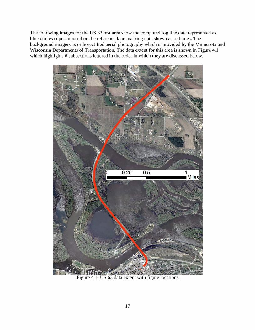
The following images for the US 63 test area show the computed fog line data represented as blue circles superimposed on the reference lane marking data shown as red lines. The background imagery is orthorectified aerial photography which is provided by the Minnesota and Wisconsin Departments of Transportation. The data extent for this area is shown in Figure 4.1 which highlights 6 subsections lettered in the order in which they are discussed below.

Figure 4.1: US 63 data extent with figure locations

18

Figure 4.2 shows an example of accurate fog line detection at location A. The offset between the calculated and reference fog lines at this location is around 2 cm. Because of this small offset, the lane stripes are not visible underneath the blue circles marking the computed fog line. Figure 4.3 shows a magnified view of the northeast side of the road.

Figure 4.2: US 63 – Location A (Data from 2 passes in each direction)

Figure 4.3: US 63 – Magnified view of location A (Data from 2 passes in each direction) (15 cm pixel resolution)

19

Location B is shown in Figure 4.4 with a magnified view of the northwest side of the road in Figure 4.5. This is another example of where the offset between the reference and computed data is small.

Figure 4.4: US 63 – Location B (Data from 2 passes in each direction)

Figure 4.5: US 63 – Magnified view of location B (Data from 2 passes in each direction) (30 cm pixel resolution)

20

Location C, shown in Figure 4.6 is an example of what happens when the vehicle passes a fork where one lane splits in to two. The gap in the computed data corresponds to the area where the lane is split. Since the fog line here is too far away from the vehicle, it is no longer captured by the system. This is intentional because the system is not designed to capture paint markings that do not represent a boundary of a standard width (12 ft) lane. Then when the new lane line starts, the camera begins to detect it again. Similar results are also common when the vehicle passes a protected right turn lane or an exit ramp.

Figure 4.6: US 63 – Location C (Data from 2 passes in each direction)

21

Figure 4.7 shows Location D which is another example of a relatively complex intersection geometry. Here, the northbound (right hand side) lane splits in to two lanes to form a bypass lane on the right side of the thru lane. Consistent with the data acquisition plan, the vehicle was driven in the right most thru lane, which in this case was the left lane of the two. Similar to Location C, the system stops detecting the fog line once it is beyond the range of the camera. The paint markings separating the thru lane and the bypass lane is a skip line which explains the pattern of the computed line in that segment. The reference data does not treat the lane marking as a skip line but rather captures it as a continuous line.

Figure 4.7: US 63 – Location D (Data from 2 passes in each direction)

22

Location E is shown in Figure 4.8 and is an example of a larger offset between the reference and computed data. Although the offset between our computed data and the reference data on the northeast side of the road is only about 2 to 3 cm, the offset on the southwest side of the road is 15 to 20 cm. A discussion of potential error sources will be found in the conclusions. It is noteworthy however, that between the two passes in a given direction, the position of the computed data is consistent.

Figure 4.8: US 63 – Location E (Data from 2 passes in each direction)

23

Location F is shown in Figure 4.9 which shows an example of an area where the system does not detect lines that are present. This can be due to a number of reasons, but the most likely reasons are poor line quality2 and a lane width that was wider than standard meaning the fog line would end up being outside the range of the camera.

Figure 4.9: US 63 – Location F

(Data from 2 passes in each direction)

4.2 MN 23 The results for the accuracy analysis of the MN 23 test area are shown in Table 4.2. Again, the passes are listed based on the order in which they were driven. The analysis includes data from 6 passes (3 in each direction) and an aggregated total for all the passes.

Table 4.2: Fog Line Data for MN 23 Pass Name Number of

Samples Mean Error [m] Standard

Deviation [m] SB 1 27635 0.065 0.038 NB 1 28586 0.040 0.045 SB 2 27818 0.065 0.049 NB 2 28567 0.038 0.042 SB 3 24772 0.061 0.038 NB 3 28423 0.039 0.041 Total 165801 0.051 0.044

Similar to the results for US 63, this analysis shows that for this test area, the system generated fog lines that were within 6 cm of those of the reference data. 2 By line quality we are referring to how the line shows up in the side-facing camera. This is different than retroreflectivity, which is a measure of how the line reflects one’s headlights. They are however related.

24

The following images show the calculated fog line data represented by blue circles superimposed on the reference data shown as red lines. Here, the reference data includes paint markings and other break lines such as edge of pavement, edge of shoulder, among others. The data extent for this test area is shown in Figure 4.10 which highlights 3 locations that are discussed in greater detail below. Locations are lettered in the order in which they are discussed. This figure contains basemap imagery from ESRI and its partners. The background imagery for all other figures in this test area are orthorectified aerial photography provided by MnDOT.

Figure 4.10: MN 23 data extent with figure locations

Location A is an intersection with a protected right turn shown in Figure 4.11. Again, there is a gap in the computed fog line where the lane forks and another gap in the data inside the intersection where there is no fog line. Note that for this test area, the reference data continues to mark the edge of the lane with a breakline (shown in red) even though there is not a physical fog line where the protected right turn lane splits from the lane of travel. The green square marks the area magnified in Figure 4.12.

25

Figure 4.11: MN 23 – Location A (Data from 3 passes in each direction) (Area in square is magnified in Figure 4.12)

26

Figure 4.12 shows the computed fog line adjacent to the protected right turn lane to show the accuracy with which the line is collected. In this location, the offsets are around 2 to 3 cm. The green square marks the area magnified in Figure 4.13.

Figure 4.12: MN 23 – Magnified view of location A (Data from 3 passes in each direction) (Area in square is magnified in Figure 4.13)

Figure 4.13: MN 23 – Close up view of location A (Data from 3 passes in each direction) (15 cm pixel resolution)

Figure 4.14 shows an intersection without protected turn lanes. Here, the gaps in the computed data correspond to the portions of the lane in the intersection where there is no fog line. The single point in the intersection is an example of the system detecting a fog line that doesn’t exist. However this point can be removed through an outlier analysis or by using some other filtering method.

27

Figure 4.14: MN 23 – Location B (Data from 3 passes in each direction)

28

Location C is shown in Figure 4.15 and magnified in Figure 4.16. This is an example of a location on MN 23 where there is a larger offset between the computed and reference data. On the east side of the road, the offset is relatively small, but on the west side the offset is around 10 cm. Again, it is noteworthy that between passes, the position of the calculated fog line is consistent.

Figure 4.15: MN 23 – Location C

(Data from 3 passes in each direction)

29

Figure 4.16: MN 23 – Magnified view of location C (Data from 3 passes in each direction) (15 cm pixel resolution)

30

5 Discussion and Conclusions 5.1 Fog Line Detection and Positioning The results of the evaluation show that generally the system will accurately determine the position of the fog lines to 10 cm or better. From time to time, the system did not detect existing fog lines, and very infrequently, it would detect a line when one didn’t exist. 5.2 Sources of Residual Error and Anomalies 5.2.1 Sensor Error Most of the results were within the 0.1 meter specification. What is described here is the source of errors less than 0.1 meters. One such error source stems from the accuracy of the sensors themselves. There is a relatively small error (around 1 to 3 cm) associated with position fixes provided by the GNSS depending on the distance to a reference station, the position of the satellites, and local geometry and interference. Additionally, position fixes are only calculated at 10 Hz, so position data must be interpolated for video frames. This interpolation assumes that between position fixes, the vehicle is moving in a straight line at a constant speed. Determining the position of the vehicle is a critical function and a prerequisite for calculating the location of the fog line. Because of this, any error in the positioning system propagates to the final calculated locations. To reduce the error in the positioning system, it would be necessary to use a GNSS receiver with a higher accuracy or to augment the positioning system with an inertial measurement unit or a distance measuring indicator. There is also some error associated with the camera’s calibration. Even for lines correctly identified within a given video frame, there still may be errors associated with the accuracy to which the camera can be calibrated. A rigorous evaluation of the camera’s calibration was not in the scope of the project. 5.2.2 Timing Ambiguity and Synchronization Another factor that affects the quality of the data is the ability to tie the sensor data together. For example, finding a feature cross section within a raw data scan is not useful unless it can be correlated to a real-world location. To do this, the time that sensors make individual readings is recorded along with the raw data. Then it’s possible to correlate the video data to the GNSS data in post-processing in order to determine fog line locations. However, there are errors in determining the times that sensor readings occur. For example, it is trivial to record the times when the video frames are received by the computer, but it is not always straightforward to record the times when the data was observed by the camera. This is because the internal clocks on the sensors can be difficult to synchronize accurately. To mitigate these errors, it would be necessary to obtain a better camera that would be capable of synchronizing its internal clock to the computer and GNSS receiver. 5.2.3 Lane Marking Visibility and Quality As discussed above, a possible system error may be the failure to detect an existing fog line. The two most common reasons for this were camera image frame limits and fog line quality. Occasionally, due to unique road geometry, the lanes were so wide that the fog line was not visible in the camera’s region of interest when the vehicle was driving in the center of the lane. To mitigate this, further improvements could be made to the camera analysis software to better

31

take advantage of the full frame. In some areas fog line quality was too poor for the software to detect. In northern climates with frequent and long-term snow plow use, the quality of lane markings can deteriorate quickly. An example of this situation is shown in Figure 5.1.

Figure 5.1: Example of poor quality fog line

5.2.4 Error vs Offset When discussing system errors, it is important to consider that the reference data isn’t completely accurate. All the errors calculated in this report are generated by comparing the computed data to the reference data. If there are errors in the reference data, this would affect the validity of the results. The stated accuracy of the reference data is 10 cm or better, so as offsets get below 10 cm, it’s difficult to determine whether errors are in the computed data or the reference data. To better account for these issues, more accurate reference data would be required. 5.2.5 Lane Re-striping In the process of investigating potential sources of errors, it was discovered that some sections of the test areas were re-striped during the time period between the collection of the reference data and our data collection efforts. Generally, the re-striping process paints the new line directly on top of the old one, but this is not always the case, which can lead to new lines not coincident with the old lines. This would affect the analysis by potentially changing the position or geometry of the lines. 5.3 Future Work The results show that the system proposed in this report can successfully detect fog lines using a side-facing camera. However, improvements could be made to the system to increase its accuracy or to develop new features. Currently, the processing software can only detect the fog line, the solid lane marking on the outside (right) side of the lane. However, it may be possible to detect and classify other types of lines determining both the type of line (i.e., solid, double, dashed) and the color of the line (i.e.,

32

white, yellow). This would be particularly useful if an additional camera were placed on the left side of the vehicle to directly collect the position of the centerline. Additionally, by classifying the line as well as detecting it, the system could determine when the left camera is viewing a road centerline, or the dashed white line separating thru lanes. In addition to detecting other painted markings, it would be useful to also identify the interface between the pavement and shoulder or the interface between the shoulder and the grass beyond it. By examining patterns and colors in these surfaces, it may be possible to detect and locate these boundaries. This system was not designed to capture information about protected turn lanes, but this data can be useful for a number of applications including driver assist systems in snow plows. If required, this data could be collected by changing the data collection procedures to include driving into protected turn lanes. Further system development could potentially negate this need by using additional cameras and software to automatically detect turn lanes in the areas adjacent to the current lane of travel. Adding a forward facing camera to the system could further expand the types of information extracted from the video data. Utilizing an additional camera in this way would allow for detection and location of other types of objects. Specifically, the ability to automatically locate road signs would be an advantage for groups collecting inventory data. Detecting other roadside obstacles, such as mail boxes, light poles, and roadside cabinets, could help improve driver assist systems. Driving the roads to collect the data is a task that requires a great deal of time. To reduce the resources required to collect this data, the data collection system could be installed on vehicles already driving the roads for other purposes (e.g., pavement monitoring/video logging vans) using the alternate set of mounting hardware. Utilizing these vehicles as a platform would allow for additional data to be collected at a relatively low incremental cost. To achieve this, more development would be required to ensure that the system would be both easy to run, so as to not overload the operator, and robust to changing conditions including extended exposure to weather. 5.4 Final Conclusions The results of this work show that the camera that was added to the data collection system was capable of detecting and locating fog lines. With the algorithms developed for this application, the fog lines detected in the two test areas were accurately located generally better than 10 cm with no manual intervention. This system can perform its function at a price point that is cost effective for wide-scale deployment and data collection. The final system used consisted of only the GNSS receiver, the camera, and the computer costing approximately $30,000 when purchased in low quantities. For those groups who seek to better characterize and digitize their road systems, these methods present a modular solution that can be utilized for data collection in a cost-effective and efficient way.

33

6 References [1] Davis, B., & Donath, M. (2014). Development of a Sensor Platform for Roadway Mapping: Part A – Road Centerline and Asset Management. (Report No. CTS 14-09). Minneapolis, MN: Center for Transportation Studies. Retrieved from: http://www.cts.umn.edu/Publications/ResearchReports/reportdetail.html?id=2376. [2] CH2M HILL. (2014). Final Report for the Minnesota County Roadway Safety Plans. [3] Minnesota Department of Public Safety – Office of Traffic Safety. (2013). Minnesota Motor Vehicle Crash Facts 2012. St. Paul, MN: Minnesota Department of Public Safety. Retrieved from https://dps.mn.gov/divisions/ots/reports-statistics/pages/crash-facts.aspx. [4] Li, Z., Chitturi, M., Bill, A., & Noyce, D. (2012). Automated Identification and Extraction of Horizontal Curve Information from Geographic Information System Roadway Maps. Transportation Research Record: Journal of the Transportation Research Board, No. 2291, 80-82. doi:10.3141/2291-10 [5] Hans, Z., Souleyrette, R., & Bogenreif, C. (2012). Horizontal Curve Identification and Evaluation. (Report No. InTrans Project 10-369). Ames, IA: Center for Transportation Research and Education. Retrieved from http://www.intrans.iastate.edu/research/projects/detail/?projectID=82223295. [6] Trimble. (n.d.). VRS Installations around the world. Retrieved April 2014 from https://www.trimble.com/infrastructure/vrs-installations.aspx. [7] Minnesota Department of Transportation. (n.d.). MnCORS GNSS Network. Retrieved April 2014 from http://www.dot.state.mn.us/surveying/cors/. [8] Trimble. (n.d.). BX982. Retrieved November 2014 from http://www.trimble.com/gnss-inertial/bx982.aspx. [9] Trimble. (n.d.). GNSS Antennas for Heavy Construction. Retrieved June 2014 from http://construction.trimble.com/products/marine-systems/gnss-antennas-for-construction. [10] iDS. (n.d.). UI-3250CP. Retrieved November 2014 from http://en.ids-imaging.com/store/ui-3250cp.html. [11] Kowa. (n.d.). LMVZ4411. Retrieved November 2014 from http://www.kowa.eu/fa/en/LMVZ4411.php. [12] Mobileye (n.d.). OEM - Mobileye. Retrieved March 2014 from http://www.mobileye.com/markets/oem/.

34

[13] Lipski, C., Scholz, B., Berger, K., Linz, C., Stich, T. & Magnor, M. (2008). A Fast and Robust Approach to Lane Marking Detection and Lane Tracking. IEEE Southwest Symposium on Image Analysis and Interpretation, 57-60. doi: 10.1109/SSIAI.2008.4512284 [14] Bertozzi, M., & Broggi, A. (1997, July). Vision-Based Vehicle Guidance. Computer, 30 (7), 49-55. [15] Stem, J. (1989). State Plane Coordinate System of 1983. (NOAA Manual NOS NGS 5). Rockville, MD: U.S. Department of Commerce – National Oceanic and Atmospheric Administration. Retrieved from http://www.ngs.noaa.gov/PUBS_LIB/ManualNOSNGS5.pdf.