development of a simplified engineering design equation ... ·...

DEVELOPMENT OF A SIMPLIFIED ENGINEERING DESIGN EQUATIONFOR A THERMOELECTRIC HEATING/ COOLING DEVICE

by ^

GEORGE ROBERT MOWRY

B. S. , The Pennsylvania State University, 1941

A MASTER'S THESIS

submitted in partial fulfillment of the

requirements for the degree

MASTER OF SCIENCE

Department of Agricultural Engineering

KANSAS STATE UNIVERSITYManhattan, Kansas

1967

Approved by

:

Major Professor

ii

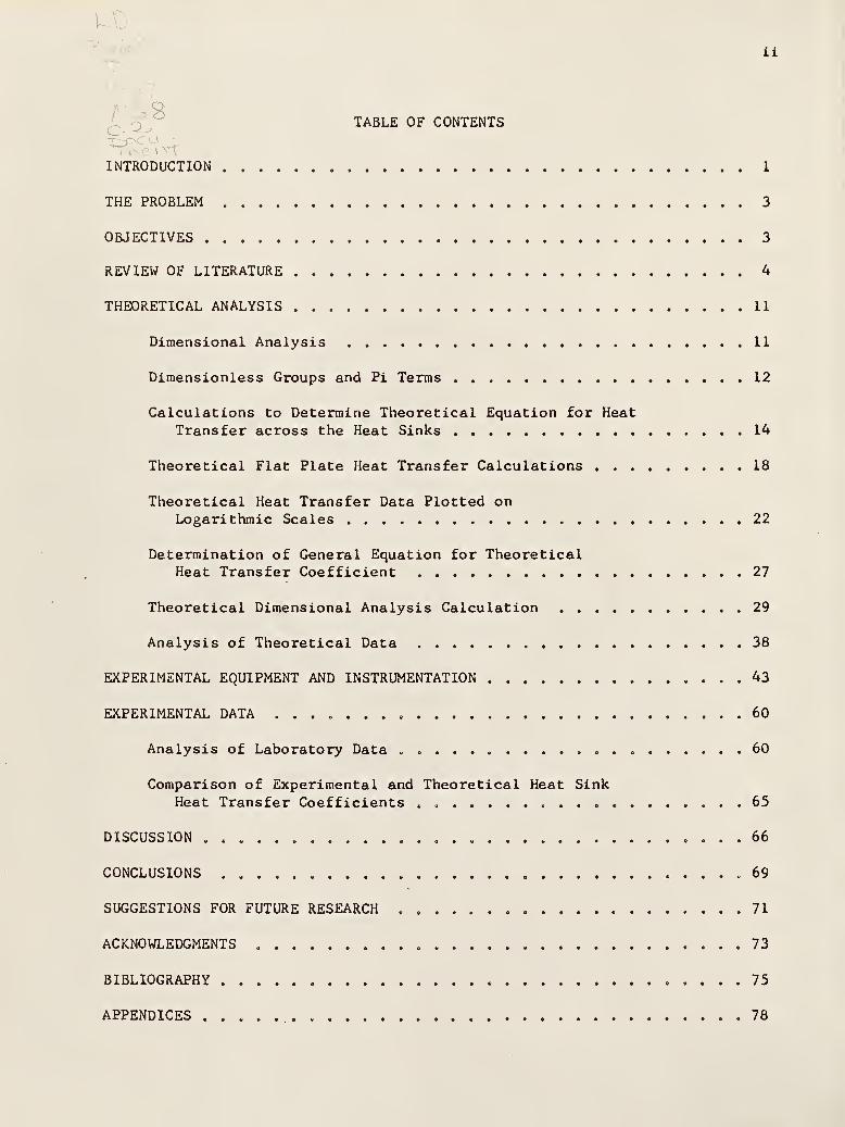
TABLE OF CONTENTS

INTRODUCTION 1

THE PROBLEM 3

OBJECTIVES 3

REVIEW OF LITERATURE 4

THEORETICAL ANALYSIS 11

Dimensional Analysis 11

Dimensionless Groups and Pi Terms 12

Calculations to Determine Theoretical Equation for HeatTransfer across the Heat Sinks 14

Theoretical Flat Plate Heat Transfer Calculations 18

Theoretical Heat Transfer Data Plotted onLogarithmic Scales 22

Determination of General Equation for TheoreticalHeat Transfer Coefficient 27

Theoretical Dimensional Analysis Calculation 29

Analysis of Theoretical Data 38

EXPERIMENTAL EQUIPMENT AND INSTRUMENTATION .... 43

EXPERIMENTAL DATA ........ .... 60

Analysis of Laboratory Data ...... 60

Comparison of Experimental and Theoretical Heat SinkHeat Transfer Coefficients . . ............ 65

DISCUSSION ...... ........... .... 66

CONCLUSIONS . 69

SUGGESTIONS FOR FUTURE RESEARCH . 71

ACKNOWLEDGMENTS 73

BIBLIOGRAPHY 75

APPENDICES .78

INTRODUCTION

Utilization of electricity on the farm and in the farm home is increas-

ing along with the development of new equipment as a result of further

application of basic principles which were discovered 50 to 100 or more

years ago. One such electro-physical principle, known as thermoelectricity,

has created interest in recent years with regard to the use of the Peltier

effect for cooling and/or heating purposes. This is the reverse process to

thermoelectric power generation (Seebeck potential) of direct current by

heating alternate junctions of pairs of dissimilar metals or semi-conductors,

the latter being required for high efficiency. Utilization of the refriger-

ating affect achieved in this manner has been limited to laboratory experi-

ments due to the minuscule nature of the Peltier effect.

A French physicist, Jean C. A. Peltier in 1834 first observed the

reverse of the thermoelectric phenomenon discovered in 1832 by Thomas J.

Seebeck, a German physicist. At that time it would have been theoretically

possible to generate electricity with thermocouples at an efficiency of about

3 percent, which would have been as good as the best steam engines available.

During the past decade or so progress in the development of thermoelec-

tric materials have produced more efficient semi-conductor compounds. Lead

Telluride is one such compound that is now being used in such applications

as water coolers, ice cube makers, air conditioners, and numerous instrumen-

tation devices. The material development has reached a plateau during the

past several years. However the method of assembling these materials into

thermoelectric junctions has continued to advance and thus further improve

the efficiency of the devices.

There is also continued advancement in mass production techniques for

assembling various numbers of thermoelectric junctions into a module. Such

techniques will further reduce the cost per Btu of cooling capacity which

will make larger thermoelectric devices more competitive with conventional

refrigeration systems.

The reverse cycle refrigeration system or "heat pump" as it is commonly

called, is capable of transferring heat from a low energy level to a high

energy level. This device can transfer more heat (Btu/Hr) than the heat

equivalent (Btu/hr) of the system power input. The ratio of the heat trans-

ferred to the heat equivalent of the power input is called the coefficient

of performance or C.O.P. of the device. A thermoelectric "heat pump" invar-

iably has a heating coefficient of performance greater than unity. At the

present state of thermoelectric material development, the cooling coefficient

of performance is usually less than unity. However it is predicted that as

more efficient thermoelectric materials are developed and better design

methods are found for applying them in heat transfer devices, a cooling

coefficient of performance greater than unity can be accomplished.

Also this transfer of heat can be accomplished by thermoelectric

devices which have no moving parts. The refrigeration effect and heat

transfer is accomplished solely by the flow of electrons through the thermo-

electric materials. Today's agricultural scientists apply new principles

and methods of heat transfer to their design needs. The improvement of

conventional systems by eliminating moving parts must be considered to be

of major importance. Several theoretically possible thermoelectric appli-

cations in agriculture are cooling milk and heating water (or air); milk

cooling and pasteurization; humidity and dew point controls; equipment

operator air conditioning; animal body cooling or heating; dehumidifiers;

electronic control element cooling, water cooling; refrigeration of semen,

antibiotics and vaccines and small isolated power supplies.

THE PROBLEM

The design of thermoelectric heating/cooling systems has heretofore

been investigated for systems that generally have somewhat fixed conditions

on both sides of the heat transfer device. Such systems are represented by

water coolers, refrigerators, air conditioners, ice cube machines and

freezers.

Methods of estimating the cooling capacity, power requirements and

other factors have utilized complicated charts and computer programs. There

appears to be very little information on engineering design equations for

determining the relationship of the important variables in a transient

system. Such a device can be represented by a milk cooler/water heater or

a milk pasteurizer/water cooler, milk cooler/water heater combination.

It would appear that a general engineering design equation which

relates the important variables would be a useful tool for the engineer.

OBJECTIVES

The objectives of the study were:

1. To investigate the development of a general prediction equa-

tion that describes the relationship of the important vari-

ables in a thermoelectric heating/cooling system.

2. To verify the general prediction equation by laboratory

experiments.

The experimental research was planned to incorporate two flat-plate

liquid heat exchangers with a 12-couple thermoelectric module mounted

between these heat exchangers. The thermoelectric module is of a type

that is commercially available at this time.

REVIEW OF LITERATURE

Only one reference has been found regarding the use of thermoelectric-

ity in agriculture. Golubyatnikov (10) reports on a thermoelectric milk

cooler/water heater unit being tested in Russia. He states,

Its relevant data are: throughput 100-150 lit./hr. (26-40gal./hr.) (or approximately 220-340 lbs./hr.) with milk storagecapacity up to 2000 Kg (510 gal.); refrigerating capacity, 2700-3000 Kcal./hr. (10,700-11,900 Btu./hr.); cooling coefficient E(CO. P.) = 1.36 - 1.92; power requirement = 0.9-2.7 KW, d.c.current I = 140 - 150 A (amperes); milk can be cooled to a tempera-ture of 8-5°C (46-4l°F) ; the energetic characteristic of the semi-conductor material Z = 1.70 x 10""-V

oC; the weight of semiconductormaterial used is 6.0-7.5 Kg. (13-16.5 lbs.); the number of thermo-couples: up to 1000.

The thermoelectric refrigerator constitutes a thermoelectricbattery of circular high-current thermocouples consisting of aternary alloy Te Bi Se negative branch and a Te Bi Sb positivebranch, connected in series. It was found that the inertia of

circular thermocouples is small, and that they can provide a highpower output with stable characteristic.

By this circular thermocouple design, resulting in muchsimplified manufacturing technology, semiconductor power systemscan be realized . . .

Golubyatnikov further describes the thermoelectric rectifier power supply

water cooler. Thermostats control the milk input and output for the device.

The milk is first pasteurized and then cooled. The heat transfer mechanism

used provides a solution of the problem of the cooling of milk with material

having a small figure of merit.

He states further,

The counter-convective heat exchange is effected (provided)by the appropriate direction of the milk and cooling water flows,

and by passing the liquid to be cooled over the radiator surfaceof the generator (thermoelectric cooler). This assures maximumheat loss and a maximum heat transfer coefficient and consequentlyan increase in generator efficiency. Thus an energetic characteris-tic Z = 1.70 x 10"3/°C obtained by the USSR Semiconductor Institute,is perfectly adequate for solving the thermal-engineering andhydromechanical problems connected with the design of an economi-cally operating thermoelectric refrigerator-heater for dairy farms.

A paper prepared by Charles L. Feldman et al. (7) explains a method by

which cascaded peltier coolers can be optimized under certain specified

conditions such as hot junction temperature. The figure of merit was assumed

-3 -1to be 2.8 x 10 K ' and T, = 300K. A low temperature freezer was designed

from theoretical calculations using bismuth telluride thermoelectric modules.

A report (1) by Dr. E. F. Cox of the Whirlpool Corporation states,

"Except for economics, thermoelectric heat pumping should be excellently

suited to distillation processes." He presents an abbreviated and simplified

theoretical analysis to determine the optimum thermoelectric material pro-

perties to maximize efficiency of salt water still operation. Several ideas

are presented for making short thermoelements and junctioning them to

bridges. The possibility of thin films of metals or semiconductors are

discussed and studies along these lines are recommended as a wide-open area

for experimental research.

A series of reports by the United States Naval Research Laboratory

Washington, D.C. (2) review the status of thermoelectric materials and

device developments. The final report (NRL Memorandum Report 1404) in

this series discusses briefly Peltier heat pumps, parameters and device

possibilities. The report states, "Materials developments now make pos-

sible the construction of practical reversible Peltier heat pumps and simple

refrigerators for a variety of military applications."

D. C. Siegla et al. (19) have analyzed the heat transfer characteristics

of a thermoelectric module for refrigeration. A one dimensional and a three

dimensional analysis are described. In both analyses the relationship of

junction temperature and dimensions of the thermoelectric element are

evaluated with respect to the heat transfer capability of the module.

In several progress reports by the Carrier Corporation to the Depart-

ment of the Navy (22), research is described relating to design of submarine

air conditioning units. An analog computer study is described which program

produces operation data based on selected values of junction temperature

differences. Thermoelectric submarine air cooling systems utilizing sea

water exchangers are estimated to be 71 percent as heavy as a conventional

reciprocating refrigeration system.

A NRL status report by Dr. J. W. Davisson and Joseph Pasternak (3)

describes theoretical analysis by analog computer programs of thermoelectric

devices for use in submarines. In each design certain factors were held

constant such as sink water temperature, air flow through cooling coil or

cooling capacity. Therefore all the important variables are not combined

into one solution.

Another NRL status report by Dr. J. W. Davisson and Joseph Pasternak

(4) summarizes thermoelectric materials characteristics and includes such

parameters as figure of merit, Seebeck coefficient, electrical resistivity,

thermal conductivity and others.

A report by E. W. Frantti, Westinghouse Electric Corporation (8)

describes the analysis of a thermoelectric air conditioning system for

submarines. Test loops were set up to measure the operating characteris-

tics of a thermoelectric module in the laboratory. Various relationships

were derived from laboratory measurements. However the relationships were

not of a mathematical form such that the variables could be combined. For

certain fixed conditions, curves are presented which, for example, show the

relationship of heat pumping rate and CO. P., to current, chill water flow

or heat sink water flow.

The transient performance of a thermoelectric couple under step-current

control is described in a paper by W. F. Stoecker and J. B. Chaddock (20).

The temperature of the cold junction with respect to time is shown following

a step-change in current. For example this characteristic is shown for

step-change from to 10 amperes and from 10 to 20 amperes and vice versa.

In all cases the hot junction temperature was held constant at 310 K.

Magazine articles by Alwin B. Newton (15) discuss the selection of

materials and prediction of performance for thermoelectric systems. Conven-

tional charts are presented which show performance for a fixed sink tempera-

ture. Analysis of other heat transfer variables is not included. The

author points out a recent development of ceramic interfaces between the

module junctions and the surface being cooled or heated. This development

has reduced the temperature drop across such interfaces from about 20 to

25 degrees F. to about an average of 2 F. Power and control systems are

also discussed.

Rajic presents in his article Refrigeration Techniques and Thermo-

electric Phenomena (18), the theoretical bases of analyzing thermo-electric

phenomena, and of the technical calculations of thermo-electric refrigera-

tion devices. To determine characteristics of thermo-electric elements,

scientists have suggested various coefficients, such as: "effective thermal

force" (E. Altenkirch), dimensionless coefficient (H. J. Goldsmid, R. W.

Douglas) and "effectiveness of thermoelement" Z (Ioffe). Z= <* © /K

where <?C is the coefficient of proportionality of the thermo-electric excit-

ing force according to Zebeke; E = OC (T - T ) where E is the voltage, T and

T - the temperature of the hot and cold junction respectively; £ - the

specific electric conductivity of the thermo-electric element, and }\ is the

coefficient of its heat conductivity. If these characteristics are known,

it is easy to determine the maximum value of the hot and cold junction

temperature (T/T ) for obtaining the maximum value of operation current

in the circuit, I . The efficiency of the refrigerating unit isoptim. J o &

determined by the refrigeration coefficient £ found from equationw max

£max= T/(T-T

o)=

E VI + Z(T+TQ)/2 - T/T ]/|yi + Z(T+T

Q)/2 + l]. Data are

given on the selection of materials for thermo-electric elements, in par-

ticular, some characteristics of semiconductor alloys Bi Te (52.8% Bi +

47.8% Te) and Sb Te, (38.9% Sb + 61.1% Te) which were studied at the

Institut Poluprovodnikov AN USSR (Institute of Semiconductors, AS USSR).

The conclusions indicate advantages of thermo-electric refrigeration over

the classical liquid one. For further successful utilization of thermo-

electric phenomena in refrigeration engineering, joint efforts of physicists,

chemists and metallurgists are imperative.

A paper by R. C. Miller et al. (14) theoretically analyzes the depend-

ence of the figure of merit (Z) of thermoelectric material on the energy

bandwidth. It was found that Z approaches zero as the bandwidth goes to

zero. The existence of an optimin bandwidth is established. However the

magnitude could not be ascertained.

A paper by Roland W. Ure, Jr. (21) presents comments on thermal con-

ductivity in two-phase alloys. Quantitative agreement between the predic-

tions of the model used and experimental data were obtained.

A paper by I. N. Pomazanov and P. L. Tikhomikov (Russia) (16) discusses

the operation of a thermoelectric/generator/ refrigerator operating from a

gas burner. With a power output of from 2 to 3KW, sufficient refrigeration

capacity was obtained to freeze about 0.7 kg (1.54 lbs.) of water per hour.

One operational disadvantage of the system described was the high rate of

flow of cooling water (100-120 liters/hr.) (26.4-31.7 gal./hr.).

In a report to the Department of the Navy (23) Carrier Corporation

research work on thermoelectric air coolers and water chillers are described,

Exact differential equations were written for heat and mass transfer rela-

tionships and these equations along with basic thermoelectric equations were

solved by an analog computer.

In these analyses fixed cooling compartment temperatures were assumed.

Figure of merit of thermoelectric materials ranged from 2.75 x 10 / C to

3.04 x 10 / C. An air cooler of about 12,000 Btu/hr. capacity was

designed and tested.

A report by the Whirlpool Corporation (24) to the Department of the

Navy describes the design of a specific prototype, including controls, of

a thermoelectric refrigerating system for use aboard submarines. One room

is held at F and another can be held at 33 F or F as may be required.

It was assumed that thermoelectric materials would have a figure of merit

of at least 2.5 x 10 / C. It was recommended from this study that a proto-

type refrigeration system be assembled and tested.

A report by the York Corporation to the Department of the Navy (25)

includes a thorough study of present food preservation and storage practices.

New food preservation methods such as freeze dehydration are discussed and

revised food storage tables were developed. Another part of this report

10

presents a preliminary study of the application of thermoelectricity to

submarine food storage facilities.

Comments by W. Maurice Pritchard in the Proceedings of the IEEE (17),

refer to previous work on calculating and optimizing the coefficient of

performance of thermoelectric cooling devices. Previous studies have been

based on the average thermoelectric properties and have neglected the

Thomson effect. Also the effects of junction resistance and a.c. ripple

in the power supply are important factors to be considered. The writer

presents a mathematical approach to the optimization problem.

A status report by Dr. J. W. Davisson and Joseph Pasternak (5) presents

thermoelectric materials data. The authors point out that no dramatic gains

in the figure of merit have been accomplished at the time of their report.

However they state that Bell Laboratories have developed a bismuth antimony

-3alloy with a Z of better than 5 x 10 at 80 K. This is a very high Z and

is a usable performance at cryogenic temperatures.

A paper by Marvin A. Fuller (9) discusses the mass production tech-

niques of thermoelectric modules. He points out that a simple flat con-

figuration which can be sandwiched between two heat sinks is desirable.

Junction resistance problems are discussed along with the process apability

level.

A report by Whirlpool Corporation to the Department of the Navy (26)

describes a design study to optimize the application of a thermoelectric

device for refrigeration aboard submarines. The study clearly showed that

it is possible and practical to thermoelectrically provide such refrigeration

in food storage rooms.

11

THEORETICAL ANALYSIS

Dimensional Analysis

The variables which influence a physical system can often be correlated

by methods of dimensional analysis. Such an analysis offers a means of

simplification by combining these factors into dimensionless groups which

can facilitate experimental research.

Dimensional analysis establishes the relationship of these variables in

a model which can then be compared with a prototype device.

To utilize dimensional analysis the variables considered to be impor-

tant to the physical system are first selected. Then these variables are

grouped into dimensionless "77"" terms.

The "77"" terms can then be related by an equation of the form:

irl

= f(72

, wr ... ^n

)

In order to determine the general equation the nature of the function

"f" must be established. Satisfactory predictions can be made if the

theoretical model and prototype are operated so that the values of the "77""

terms in each case are equal.

The method of evaluating the function "f" is to hold one of the inde-

pendent "77"" terras constant and vary the other. This method is then applied

to each of the "77"" terms and the resulting component equations can be

combined to give the general relationship. The final equation may be a

polynomial type or exponential type depending on the relationship of the

"77"" terms.

12

Dimensionless Groups and "Jfu Terms

The design of this investigation was developed around the principles of

dimensional analysis. The formation of dimensionless groups was investi-

gated with an IBM 1620 computer to provide theoretical data. This data was

supplied to an IBM 1410 computer which was programmed to statistically

analyze the data. The output from the 1410 computer yielded a general

prediction equation which could be experimentally investigated.

In analyzing the dimensionless "77"" groups the following variables were

considered to be pertinent:

Factor Description Dimension

Mass-Length-TimeTemperature Units

wb

Ati

Atc

Wc

W,

Cooling capacity

Power required

Difference between inlet watertemperatures

Drop in water temperature dueto cooling

Water flow rate through cooling sink

Water flow rate through heating sink

2 -3ML T

°

2 -3ML T

9

MT-1

MT-1

The required number of U 7T" terms can be determined as follows:

P = K(Q )

a, <At.)\ (At )

C, (W )

d, (W, )

e

wb x: l c c h(1)

Substituting the dimensions for each term:

ML ML2\a• 6". •'• $• (ff

(2)

13

Equations can then be written by summarizing the exponents for each

dimension as follows:

£M: 1 = a + d + e (3)

2L: 2 =* 2a (4)

£T: -3 = -3a - d - e (5)

£3: = b + c (6)

From these equations the following is obtained:

a = 1

d + e = or d=-e

c = -b or b = -c

Substitution of the above values into equation (2) yields:

From equation (7) by rearranging terms the following results:

h -# fey

The relationship between the three "77"" terms thus formed can be

analyzed by holding one constant while the other two are varied. The

analysis was developed as follows:

First set of data from computer:

"l m f (^"2 * 3* wne re; (77" constant

Q At. W77- =-c- 7T = —i 7T=-£-' 1 P ' " 2 At ' "3 w\

wb c h

14

Second set of data from computer:

TTl

= f ( 7T , T2

) ( 7T2

constant)

In the analysis another "jf" term was used as a level indicator to cor-

relate differences in cooling capacity and water inlet temperatures on the

cooling side. The fourth "77"" terra was as follows:

T77" - wic _ inlet water temperature on cooling side4 t drop in water temperature due to cooling

This "77"" term was held constant at four different values of inlet

water temperature while At was held at a constant value of 2 F. The

relationship between the other "7f" terms was then determined at these

levels. The data were then combined to yield a general prediction equation.

A family of equations of surfaces can be obtained for various values of At .

Engineering design can begin by selecting a value of At and then using the

general prediction equation the other pertinent variables can be related.

Calculations to Determine Theoretical Equation forHeat Transfer Across the Heat Sinks

Basic Equation :

. .Atq- k A^

15

Values of Thermal Conductivity - "k"

MaterialBtu : Gm. Cal.

hr.'ft. • F./ft. : sec. 'cm. ' C./cm,

Copper 222.0 0.918 (1)

ruN^?

n^ °' 145 °- 0006 (2)

(Monofilament)

SiliconeGrease

Dow Corning# 340

0.363 0.0015 (3)

(1) At 18°C. - Handbook of Chemistry and Physics, Twenty Fifth Edition.

(2) At 68 F. - Elements of Material Science, by VanVlack. Second Editionby Addison Wesley, 1964, p. 420.

(3) Dow Corning Corporation, Bulletin # 04-027, September 1963.

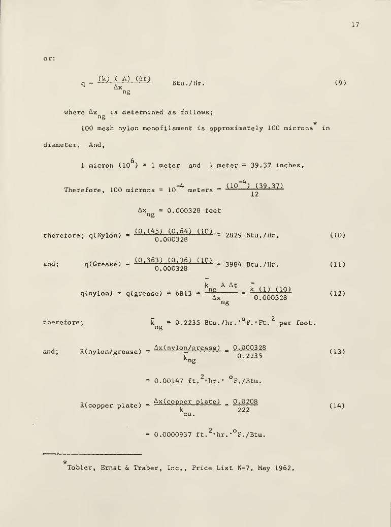
Figure 1 shows the cross sectional view of the heat sink copper plate

and the nylon/grease separator between the heat sink and the thermoelectric

module. The total area considered in these calculations is one square foot,

100 mesh nylon material has an open area of approximately 36 percent.

Therefore the nylon occupies 64 percent of the area and the silicone grease

fills the remaining 36 percent.

Assuming a ten degree F. temperature difference across the nylon and

grease separator the following calculations are considered:

thermal percent of temperature, _ , conductivity area differenceheat transferred = —„. . .

t~~z : : "

thickness of nylon/grease separator

Tobler, Ernst & Traber, Inc., Price List N-7, May 1962.

I FT.

16

COPPER PLATE

7YzzzzzzzzzzzzzzzMmmNYLON64%

GREASE*k— 36% A

—.0208 FT.

— .000328 FT.

Fig. 1. Cross section of heat sink copper plateand nylon/grease separator.

17

or:

=<kM A? W

^ Ax

where Ax is determined as follows;

100 mesh nylon monofilament is approximately 100 microns in

diameter. And,

1 micron (10 ) = 1 meter and 1 meter = 39.37 inches.

-4_4 qo ) (39 37)

Therefore, 100 microns = 10 meters = J ~~—*

—

Ax = 0.000328 feetng

therefore; q(Nylon) =( °' ^OOO^ ^ = 2829 Btu * /Hr ' (10)

and; q(Grease) = ^63^0^ (10) . 3984 Btu#/Hr> (n)

q(nylon) + q(grease) = 6813 = -*fc—- = ^^^f (12)

ng

therefore; k = 0.2235 Btu./hr.* F.'Ft. per foot.ng r

„ j o/ i / \ - Ax(nvlon/grease) m 0.000328 ....and; R(nylon/grease) = —*—*—=-J& u (13)

Kng

= 0.00147 ft.2'hr.« °F./Btu.

d/ i n Ax(copper plate) 0.0208 ....R(copper plate) = —*—

*£K fc = —^

—

(14)cu.

= 0.0000937 ft.2'hr.*°F./Btu.

Tobler, Ernst & Traber, Inc., Price List N-7, May 1962.

18

R = 0.00147 + 0.0000937 = 0.0015637 (15)

and

C = h = » m ? CA» = 639.5 Btu./ft.2'hr.'°F. (16)

R 0.0015637

therefore;

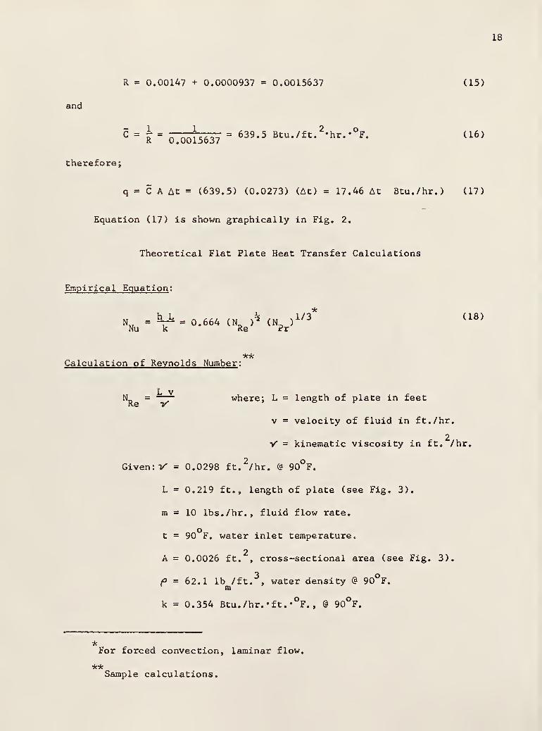
q = C A At = (639.5) (0.0273) (At) = 17.46 At Btu./hr.) (17)

Equation (17) is shown graphically in Fig. 2.

Theoretical Flat Plate Heat Transfer Calculations

Empirical Equation :

Nu k Re Pr

Calculation of Reynolds Number :

L vN = -~r where; L = length of plate in feet

v = velocity of fluid in ft./hr.

2V = kinematic viscosity in ft. /hr.

Given: Y = 0.0298 ft.2/hr. @ 90°F.

L = 0.219 ft., length of plate (see Fig. 3).

m = 10 lbs./hr., fluid flow rate.

ot = 90 F. water inlet temperature.

2A = 0.0026 ft. , cross-sectional area (see Fig. 3).

P = 62.1 lb /ft. , water density @ 90°F.m

k = 0.354 Btu./hr. 'ft.^F. , @ 90°F.

(18)

For forced convection, laminar flow.

**Sample calculations.

19

lO ^ lO CM —

3 S33y03a-3DN3ii3ddia 3ynivy3dW3i

CO uX

3 ^"O •

3B AJ

CQa•** Cu •|H

aj

o (0

(J »*.—

«

Q- o VX g

-

^*J» a> T>~) j= c\— aj CO

CO *0 .

C u,i <0

10

n W 

-Jaj

•o

o <0

oc•H

z x.03_ c •»-l

—J V

o a3 AJ

o AJ

a><l

u uso

0) >-l

C£ oc

o a> 3>»</

»-

AJ j=a>w •

o CO

0) >jraJ 0)

cU-l oo

AJ

AJ uo c—

1

1

3Pm •»-»

00

20

<fy7777777777777/A

.219 FT.

. /./ z s.-jcszz ZZ

.021 FT.

SIDE VIEW

n.125 FT.

'!'.'.1 1

!tr ' •-

-i

i

|

•

>-

END VIEW

Fig. 3. Dimensions used for theoretical flat plate

heat transfer calculations.

21

then;

Volume of water .. ., , _., _ ,, .. lbs./hr. 10 , 1Q *

flowing - v - - - rrrrrr ,, . : c 19

;

£ ^ 3, /o^o^\ /iu /r- 3 (3600) (62.1)ft. /sec. (3600) (lb /ft.

IQ

V = 0.00004477 ft. /sec.

and;

Velocity offt.

3/sec. (3600) _ 0.00004477 (3600) ,__.

water tlowing = v = —•—

«

*—

J

r4- = -1

nAoA (20)-„ ,, cross-sectional 0.0026ft./hr.

area

v = 61.9 ft./hr.

then;

. L^ a (0,219) (61.9) =(\e V 0.0298 ^

'* ^

and;

N_ = 5.23Pr

**Calculation of Heat Transfer Coefficient :

NM = 0.664 (N_ )* (N_ )

1/3(22)

Nu Re Pr

= 0.664 (454.9)^ (5.23)1/3

= 0.664

= 24.59

then;

h =CV ) (k>

= (24.59) (0.354)L 0.219 (23)

h = 39.75 Btu./hr.-ft.2'°F.

**Sample calculations.

22

The theoretical values of the heat transfer coefficient are shown in

Table 1. These values are shown graphically in Fig. 4.

Theoretical Heat Transfer Data Plotted onLogarithmic Scales

The data obtained from the theoretical analysis of flat plate heat

transfer were plotted on logarithmic scales. Graphs of equal water tempera-

tures (60 F. , 75 F. , 90 F. ) were obtained by plotting the heat transfer

coefficient versus the mass flow rate. These data plotted as straight lines

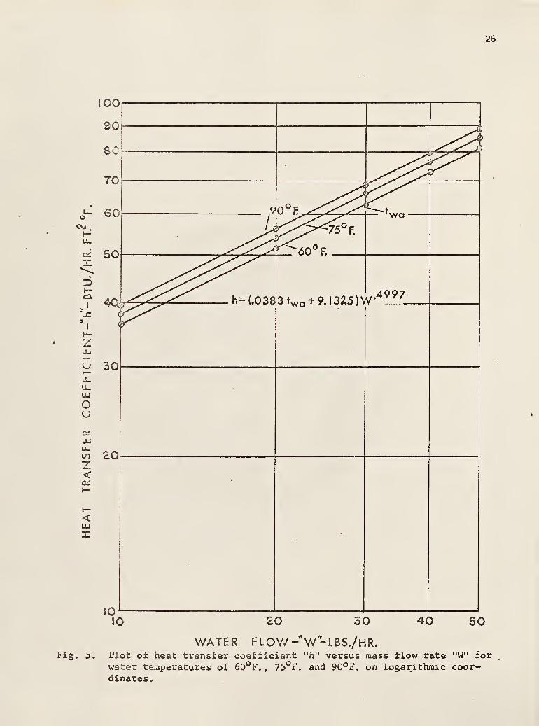
on logarithmic coordinates as shown in Fig. 5.

From this data equations for each water temperature line were obtained

as follows;

Equation is of the form: y = bxm

Determination of the slope :

m -log y

2- log y

l

log x2

- log xl

= log 68.83 - log 39,7501

"

log 30 - log 10

from calculations:

y. = 39.75 and x = 10

y2= 68.83 x

2= 30

= 1.83778 - 1,59934 =m1.47712 - i.o

u.*yy* (24)

Determination of "y" Intercept

y = bxra

(25)

Therefore; b = —*• or log bm ° = log y - mlog x

And for x = 10

23

u0)

U4id

ccd

I-

4J

4J

'.w

•J

43

i—

i

«u •

•rt oi-J aj

0) <fl

•m —1O aO43 ^•U 4->

cx; a)

w •Hf> oD H

CH« 14-1

U <UCO oQ cj

.OCH

D4-)

CO

uuCtJ

5-.

o

cj

CO

43CO

•Hl-l

(0

>

• -H o o 00 COCn co r^ r- m oo5

• • • • •

O <r in <t Csl ooON CO co vD -d- vD

--4 i—

t

COi—i

• r* vD vO CO ooU4 oo CO CM vO r*>

• • • • •

m CO m o •—i mr* CO 00 <f <r vO

CX4

oovO

U-,

oon

[14

m

U4

ovO

(X4

Oon

m

mvO

COCO

m•

o>oo

CM

ooon

ONoo

-a-

CMvO

moo

ooo

COCM

mCOCM

o

COCM

on

r-4

vO

ON

vO

• mu. m r*

• •

o <r ftv£> <r nO

oON

•

COCOON

o00

ONoON

ovO

o•

CMCMvO

ON•

m

ONo

•

oooCO

CO

CO

O

CO

ONON

COCO

00

COCO

ONm

CM

COO

CM

COCM

mCM

OCM

•

vOm

COm

o

m

m

ONCO

00ON

CO

CM

vOCO

1 ,

co

wco

CO

•

= fX4

O U 0) (!) 4301 -4 0) —

<

.-4 IT •

u 4-1 l-l c C ICNV X! CO 0) o l-l 1

4J w 5 43 •H ct> •l-l M 4-1 4-»

<0 E CO 43 CO CJ C cws . 14-1 3 c e C CM a) .

o o Z 0) 3 0) CO i-i •

U-l CD • E Z E c CJ Mco >, U C4 •M •H CO •h j:^ 4-J 43 "O a 4-1 a u CW >v

CUCO •r-t ^ 1—1 S-o' <—

(

v^ H U-l •

e • o • O 0) %Z CO z CO O CQO CD CD a 0)

> > Oi z X

[XI

24

<D

U

4-1

«01-1

CJ

QEcju)-i

CJ4Jc3

"OcCO

a)xj

<o

u-t

o

o

Cx,

O

[x,

Cx,

oo

CM

o

43

CO

X

O

[x,

mr-

coo

XS3

H

[nOovO

o

u[X,

X•Hu

>

LA r* vO . oCO LO LO on CO Cxi ON /—

\

• * • • • O v»< •

CO on >J <f co o fxi

CM o f>. m co a% <f OCN en CM

CMCOo>CMO

*

o

men

•

o

Pxi

OC7\

enCN

mi—

I

en en in en Oi—

1

on <r r*» on 0* in A• • • • • •-N r*» /~\

CO CO o m <r /—

\

• N.X •

CN o o m co • [XI Fxi

CN en onOoON

1—

<

•

Oin

vOmen

en

o

Om

o

m co \0 CM o • vOr-« m m sr r^ vO • Pxi

• • • • • o O #>

CN CO vO CM o A O /-N

CN o m m co ^-\ a «£• •

CN en m •

oin

•

Pxi

OovO

enen

•

o

[X|

ovO

oCO vO vD CM <f ii

•

o vX vX •—I St • en CO• • • • • CM «tf *~s

cy» r~ on on ON vO o ft* II

r^ vt •—

i

<t r- • o*-4 CN 00

i—i

OovO

oII

u

CM

4-t

CW

•

x;

CO

CO

CJ1—1

co•H

ON <r -3- GO vO *>. •v. CO

*tf i—i en o on <r CM 3 c• • • • • • • 4-1 CJ

CO r^ o co m CM 4J CO Er>- <f CM <t r- vO <+-l v«/ Hw4 CM in

r-t

<r en

II

/—

\

en

4JCW•v.

4-1

•HCO

oCJ

(0

4J•H>•H4JCJ

3

oOS

2>—^

MCJ

CN CO CM ON CM E •i-l -a X• • • • • X > c E

co vO m vO CM —i o 3r- >* <tf <f f>» v-* O o 2f—

•

CM CN

*-* ^-N

4J•HCO

c

o

•H

CO

c•H

r-l

CO

CJ

x;H

•—I

4JTJCCO

MOi

vO1 1

CO

CO

CO

CO-

•

Cxi

CO

o u CJ CJ io o1 -H CJ •—

I

1—1 ; • 4J>-l *J u c c ICN oa> !< CO CJ M I • CO

4-> —

'

2 X •1-1 CJ •r-l S-. *J 4-1 (XI

CO E CO JO CO a) C U-l

5 • <+-) 3 c E c U-l CO • uo 2 CD 3 <D CO •H • CD

M-l CJ • E 2 E c o M X,O CO >. u co •H •H <0 •H J2 4J

-«* 4-> X TJ O 4J o ^ M-l -s. oCJen •H ^. I—

1

^/ t—

1

s^/ H M-l *

E • CJ • o <0 CD 3 CD 33 4J O 4-> c oi CO 2 4-t O 4J»-l 4-1 i—

i

l4-( >,2 CO 2 (0 U PQo CJ 0) 3 0)

> > OS 2 K

25

<7>

OO

in<7>

O0>

o

o>

uV)

u>

<a

e

"Oc«

1-1

3

4

0)

a.

CO uj

O £uj S>

Q *w

o i 300 LU

rvi 

H- z

< MrVm LU

h- a. 0)

m

LU

a:LU

inin

in in :nmSm inin <*•

'J 332030313' ^H/'nig-H,rlN30IJd303 a3dSNVai 1V3H

0) •

oo •»->

cdLi —ia) a.

1-1

a.a.ou

CD4J

a) c.c -•

«M•H<o <o

-4 uO uO 0) ^M

1_1

26

ZLU

u 30

UJ

Ou

oo 20Z<

<UJ

X

Fig. 5.

10

h= (.0383 twa + 9. 1 325 )W499>7.

20 30 40 50

WATER FLOW-"W-LBS./HR.h" versus mass flow rate "W" for

water temperatures of 60°F. , 75°F. and 90°F. on logarithmic coor-dinates.

Plot of heat transfer coefficient-vOc tcO

27

log b = log 39.75 - 0.49974 log 10

log b = 1.59934 - 0.49974

log b = 1.09960

Therefore: b = 12.58 ("y" intercept)

Equation of the line, heat transfer coefficient vs. flow rate for water

temperature of 90 F. is:

_ .. QQ 0.4997y = 12.58 x

Similarly:

Equation of the line, heat transfer vs. flow rate for a water temperature

of 60°F. is:

... ,, 0.4997

y = 11.43 x

Determination of General Equation for TheoreticalHeat Transfer Coefficient

From previous calculations it was determined that the slope of each

water temperature line was approximately equal. The temperature of the

water caused the lines to move vertically on the graph.

The calculations also showed that they intercept changes in equal seg-

ments for each equal segment of change in water temperature. Therefore the

following relationship was noted:

For 90 water temperature b. (y intercept) is 12.58.

For 60 water temperature b (y intercept) is 11.43.

and; Ab = b - b = 12.58 - 11.43 = 1.15

Dividing Ab by 30 yields a value of "b" for each degree change in water

temperature.

28

Therefore b. 0p would be 11.4683; b, would be 11.5066, etc. If the

above were true from F to 60 F then multiplying the water temperature by

.0383 would yield the correct b (y intercept). However the following was

noted:

(60) (.0383) = 2.2980 (for 60°F water temperature)

Subtracting 2.2980 from 11.43 (b,^0lJ = 9.132OU r

Similarly:

(90) (.0383) = 3.4470 (for 90°F water temperature)

Subtracting 3.4470 from 12.58 (b o p) = 9.133

Therefore the constant 9.1325 must be added to each water temperature

multiplied by 0.0383.

The mathematical relationship was determined to be;

b = (0.0383) (water temperature) + 9.1325

The general equation used to relate water flow, average water tempera-

ture and the heat transfer coefficient was;

4QQ7y = (0.0382 t + 9.1325) x '

**'(26)

wa

where;

y = heat transfer coefficient - Btu./hr.ft. F.

ot = average water temperature - F.

x = water flow rate - lbs./hr.

29

Theoretical Dimensional Analysis Calculations

Assumptions ( 77 Constant):

Twic = 90°F.

At = 2°F.c

-rr _ Twic _ 90 _ , c . ...If , = r-— = — = 45 (constant)

4 At 2c

W7f . - -f-

= 0.5 (constant)3 w,

a

W = 10 lbs./hr.c

Total cooling capacity;

Q = (W ) (At ) = (10) (2) = 20 Btu./hr. (27)c c c

Cooling capacity per couple;

c 20

% =(12) (3.413)

=(12) (3.413)

=°' 488 Wa" S (28)

Outlet water temperature on cooling side;

Twoc = Twic - At =88 °F. (29)c

Temperature of plate on cold side;

From previous heat transfer relationships it was shown that;

Qc= h A At

lnor h =—

-

(30)

In

Also,

4997y = (.0383 t + 9.1325) x ' (Equation 26) (31)

30

Also it is known that,

h = y

Therefore,

Q-= (.0383 t + 9.1325) x

,4" 7(32)

A At, waIn

where

,

At, -*In (Twic - t )

, pc(Twoc - t )

pc

and,

x = W ; t = t + At, ; Twoc = Twic - Atc wa pc In c

therefore by trial and error substitution for t equation (32) and bepc

solved and the solution is;

o *t = 70.72 F.pc

Temperature gradient across nylon, grease and copper plate;

QAt = TT7I = 7^TZ = 1.1455 °F. (33)

eg 17.46 17.46

Temperature of cold junction;

t r = t - At = 69.5745 °F.* (34)cf pc eg

t = 5/9 (t , - 32) = 20.8747 °Ccc cf

IBM 1620 computer data.

31

Temperature difference between hot and cold junctions;

1.13 + .00678(t ) - qAt. = n ._,

CC ~ = 44.5001 °C. (35)he .0176

Temperature of hot junctions;

t, t + At, = 65.3748 °C. (36)he cc he

t. - = (9/5) (t, ) + 32 = 149.6747 °F.*hf he

Millivolt drop across each couple;

V = .526 (At. ) + 43.4 = 66.8071 MV. (37)ra he

Total power required for module;

[V + (.017) (I) (t )] [(12) (I)] •P = —

1 „nnCC

= 12.9834 watts (38)w 1000

P . - (P ) (3.413) = 44.3124 Btu./hr.*wo w

Total heat to be rejected at hot junctions;

Qu = Q + P U =20+ 44.3124 64.3124 Btu./hr.* (39)h xc wb


At = t—tt = 3.6834 °F. (40)eg 17.46

Temperature of plate on hot side;

t .= t. . - At = 145.9913 °F.* (41)

ph hf eg

Water flow rate through hot side;

Wc 10

Wh

= ^ = -^ = 20 lbs./hr. (42)

32

Temperature rise of water through hot side;

h o *At

h= — = 3.2156 °F. (43)

h

Inlet water temperature at hot side;

From previous heat transfer relationships,

Qh= h A At or h = j-jj- (44)

In

and,

4997y = (.0383 t + 9.1325) x (Equation 26) (45)

wa

and it is known that,

h = y

where

,

AtIn (Twih - t , )

, ph(Twoh - t . )

ph

and,

x = W, ; t = t . - At.h wa ph In

therefore,

Qh 4997-= (.0383 t + 9.1325) x '**'

(46)A At, wa

In

and by trial and error substitution for Twih equation (46) can

be solved and the solution is,

Twih = 104.7413 °F.*

33

Outlet water temperature at hot side;

Twoh = Twih + At = 107.9769 °F. (47)n

77 = —£ = —2S = 4513*

(48)

wb

^ . Twih^- Twic , 104,7413 - 90, , 7>37Q7* ^

c

WT

->

= 7T = ™ =' 3 (constant) (50)

3 Wh

20

77/ = 77— = — = 45 (constant) (51)

c

Assumptions ~ff Constant:

Twic = 90° F.

At = 2° F.c

-rr TwJC 90 . _ .

II . = T~— = ~ = 45 (constant)

Twih = 110° F.

_. _ Twih - Twic _ 110 - 90 _ .. , ...77

2=

— = r 10, ^ constant )

c

W =10 lbs./hr.c

A = .0273 ft.2

Calculations:

Total cooling capacity;

Q = (W ) (At ) = (10) (2) = 20 Btu./hr. (52)c c c

34

Cooling capacity per couple;

= 0.488 watts (53)Nc (12) (3.413)

Outlet water temperature on cooling side;

Twoc = Twic - At = 90 - 2 = 88° F. (54)c

Temperature of plate on cold side;

From previous heat transfer relationships it was shown that,

Qc= h A At or h = —- (55)

In

Also,

4997y = (.0383 t + 9.132) x * (Equation 26) (56)J wa ^

Also it is known that,

hSy

Therefore,

Q.

= (.0383 t + 9.132) x,4"7

(57)A At, wa

In

where,

At. -*-In (Twic - t )

, PC1

(Twoc - t )

pc

and,

x = W ; t = t + At, ; Twoc = Twic - Atc ' wa pc In <

35

therefore by trial and error substitution for t equation ( 57) canPC

be solved and the solution is;

t = 70.72 °F.*pc


QAt = T7TZ = 7TZZ = l « 1455 ° F - (58)

eg 17. 46 17.46

Temperature of cold junctions;

t . = t - At = 69.5745 °F.* (59)cf pc eg

t = 5/9 (t , - 32) = 20.8747 °C. (60)cc cf

Temperature difference between hot and cold junctions;

1.13 + .00678 (t ) - q ^At = cc c m 44#5001

°c# (61)

he .0176

Temperature of hot junction;

t. t + At. = 65.3748 °C. (62)he cc he

t, . = (9/5) (t. ) + 32 = 149.6747 °F.*hf he

Millivolt drop across each couple;

V = .526 (At, ) + 43.4 = 66.8071 MV. (63)m he

Total power required for module;

[V + (.017) (I) (t )] [(12) (I)] •P = ~

, nnnCC = 12.9834 watts (64)

w 1000

*IBM 1620 computer data.

36

P ,= (P ) (3.413) = 44.3124 Btu./hr.* (65)wb w

Total heat to be rejected at hot junctions;

Qu= Q + p u

~ 64.3124 Btu./hr.* (66)h c wb


Q,

At = 777t = 3.6834 °F. (67)eg 17.46

Temperature of plate on hot side;

t ,= t, . - At = 145.9913 °F.* (68)

ph hf eg

Water flow through hot side;

From previous heat transfer relationships;

QhQ = h A At, or h = ;

" (69)xh In A At,In

and,

4997y = (.0383 t + 9.132) x *

**'(70)J wa

and it is known that,

h = y

where,

At,

At'h

T ; x = W, ; t = t . - At.) h wa ph InIn (Twih - t . )

' h wa ph, phin

(Twoh - t . )ph

and;

37

^h 49977—^— = (.0383 t + 9.132) x * *' (71)A At, wa

In

therefore by trial and error substitution for w, equation (71

)

can be solved and the solution is;

Wh

= 25.35 lbs./hr.

Temperature rise of water through hot side;

Qh _ *At

h= ~ = 2.5370 F. (72)

h

Outlet water temperature at hot side;

Twoh = Twih + At, = 112.5370 °F. (73)n

Therefore;

QT = =-* = .4513 *(variable) (74)

wb

^2 = TWlhA t

TWi ° = 10 *° *< constant > (75)

W7", * — 0.3945 *(variable) (76)J W

h

7/*

4= —^ = 45 *(constant) (77)

c

38

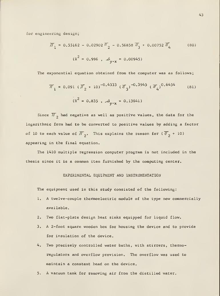
Analysis of Theoretical Data

The theoretical data acquired from the IBM 1620 computer were pro-

grammed for multiple-regression analysis by an IBM 1410 computer. Plates

X and II graphically show the theoretical data* Appendix C shows the data

furnished the IBM 1410 computer.

The following equations were used for the statistical analysis:

= A + B T + C 7T + D J.2 3 4

= A + B 7T- + C J- + D 7T, + E 7T 7" T.2 3 4 2 3 4

= A + B72

+ C 7f + D7"4

+ E 7T2T^ 7T

h+ FF

4'

1. If

2. ri

3. Wl

4. Wl

5. 7Tl

6. 7Tl

7. wl

= a + b w2

+ c j3

+ d ^2r3irk

= A+B^2+C7

3+ D7

4'

= A + B 77* + C 7T_ + D /7". + E 7"/2 3 4 4

2 3 2 3 4 4

The data also were converted to natural logarithmic values. These

values were also processed by the IBM 1410 computer for the best fit analy-

sis of an equation of the form;

log 77^ = A .+ BlogT2+ Clog7*

3+ Dlog7"

4(78)

From equation (78) an equation of exponential form can be derived as

follows;

77*, = eA

(/7\)B (7T )

C{7T,)^

1 2 3 4(79)

From the multiple regression analysis by the IBM 1410 computer the

following polynomial equation was determined to provide adequate precision

EXPLANATION OF PLATE I

Plot of the computer data of the pi term Q /P . on the pi term

CT ., - T . )/At while holding the pi term W /W, constant andN wih wic c ° r chthe pi term T . /At constant at four values,

wic c

40

wH

1

.{£>

CM

CO

^

*•

Si

CMi

£h-v_^

O. .

tf*

CM1

<fri

<DI

CO1

1wd/D-({*)

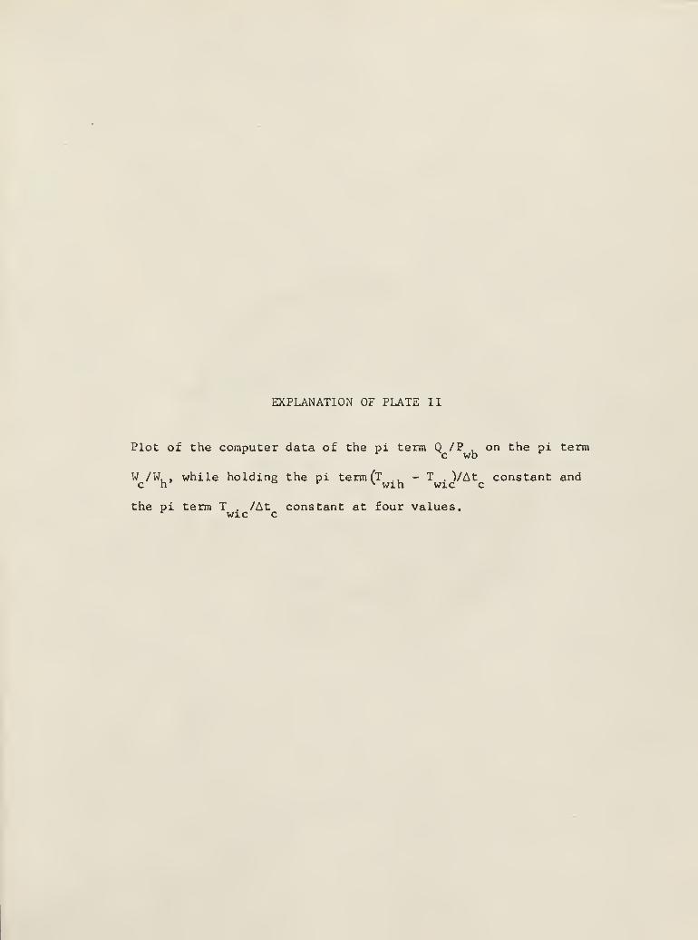
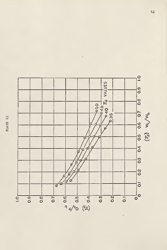
EXPLANATION OF PLATE II

Plot of the computer data of the pi term Q /P on the pi term

W /W, , while holding the pi term (T . , - T . VAt constant andc h o r \ W1h W1C c

the pi term T . /At constant at four values.r W1C c

42

wH

0) o Is*. o m 4- IO <V1

•

o o o o o o o o

V'o W

43

for engineering design;

7fl

= 0.55162 - 0.02902 7T - 0.56858 7^ + 0.00752/7^ (80)

(R2

= 0.996 , 4> = 0.00945)yx

The exponential equation obtained from the computer was as follows;

Tx

= 0.091 (7T2

ID)"' 4333 C^)- - 3945 (

4̂)°- 6454 (81)

(R2

= 0.835 , ^ = 0.13641)yx

Since 77~_ had negative as well as positive values, the data for the

logarithmic form had to be converted to positive values by adding a factor

of 10 to each value of 7T , This explains the reason for ( 7"^ + 10)

appearing in the final equation.

The 1410 multiple regression computer program is not included in the

thesis since it is a common item furnished by the computing center.

EXPERIMENTAL EQUIPMENT AND INSTRUMENTATION

The equipment used in this study consisted of the following:

1. A twelve-couple thermoelectric module of the type now commercially

available.

2. Two flat-plate design heat sinks equipped for liquid flow.

3. A 2-foot square wooden box for housing the device and to provide

for insulation of the device.

4. Two precisely controlled water baths, with stirrers, thermo-

regulators and overflow provision. The overflow was used to

maintain a constant head on the device.

5. A vacuum tank for removing air from the distilled water.

44

6. A return tank and a supply tank with suitable pump.

7. A d.c. power supply consisting of two six volt automobile type

batteries connected in parallel and two rheostats to control the

current.

8. A thermocouple switch.

9. An electronic ice bath.

10. A precision potentiometer.

11. An ammeter and voltmeter.

12. A precision balance to batch weigh the liquid.

13. Needle valves to control flow rate.

14. Liquid filters and associated apparatus.

15. Calibrated thermocouples for determining the water temperatures

and degrees of cooling and heating of the water by the device.

16. Thermocouples soldered to junctions to determine hot and cold

junction temperatures.

The liquid heat sinks were made of copper. The heat sinks were approx-

imately 1.5 inches wide by 2.25 inches long so as to fit the heat transfer

area of the thermoelectric module.

A mixing tube was attached to the outlet of each sink. The purpose of

the mixing tube was to assure adequate mixing of the liquid before the out-

let thermocouple sensed the liquid temperature. The mixing tube was made

from one-half inch diameter copper tubing. Inside the tube and at one end

a small copper disc was suspended by means of thin spiders in the center of

the tube. Liquid flowing through the tube had to pass over and around this

disc thus causing turbulence and subsequent mixing of the liquid. A cross-

section of the device is shown in Plate III. Plate IV is a photograph of

EXPLANATION OF PLATE III

Cross-section of thermoelectric heating/cooling device showing

arrangement of thermoelectric module, heat sinks inlets and out-

lets, thermocouples and associated equipment.

46

PLATE III

LIQUID OUT

%" COPPER TUBE

LIQUID ISM

THERMOCOUPLE

THERMOCOUPLE

V-i mum

THIN COPPEPLATE

szsgsa titf

MODULEE7ZZZZZZZZZZZZZZ

2H I t t I I I I

LIQUID

o-j

THERMOCOUPLE

MIXING CHAMBER

PLASTIC TUBE

COPPER HEAT SINK

2 POWER LEADS

MIXING CHAMBER

THERMOCOUPLE

^w LIQUID OUT

EXPLANATION OF PLATE IV

View of thermoelectric heating/cooling device mounted inside

plywood container and ready for addition of insulation

material.

PLATE IV

48

**-—^ .- -- *-r-vrpv- f^"V^iiYwy.-.>y ~ry~~..»* . y —*~t- —

il. II I. Ill J.l.i Jri.l.nlllli' fc-^ ,— -at -.1 nV»j~~*ii*«»~~i»^~

49

the device mounted inside the plywood container and ready for addition of

the insulating material.

Short lengths of plastic tubing were used to connect the inlets and

outlets to 3/8 inch diameter copper tubing which connected to the water bath

outlets.

The block diagram of the laboratory equipment is shown in Plate V. The

water baths were equipped with overflow outlets which provided the device

with a constant head of water. By this system of overflows precise rates

of flow were possible to attain and hold constant. Each water bath con-

tained an electric stirrer and a precision mercury actuated thermoregulator.

The mercury actuater was electrically connected to a solid-state, low cur-

rent actuated, 5-ampere capacity relay. This relay controlled the power to

the 300-watt low time lag water heaters in each water bath. Each water bath

outlet was provided with a fiberglass water filter. Plate VI is a photograph

of the experimental system as it appeared in the laboratory.

A twenty gallon plastic supply tank was provided to furnish the dis-

tilled water for both water baths. Water could be circulated through a

heat exchanger before going into the water bath is a lower water bath temper-

ature was required. Water entering the water baths was maintained several

degrees cooler than the desired water bath temperature. The water bath

heaters then heated the water to the desired temperature and turned off as

determined by the thermoregulators. Cooling water was obtained from a

standard electric water fountain type cooler.

A vacuum tank was constructed from a liquified gas cylinder. A vacuum

pump was used to obtain a high vacuum (about 28 inches Hg. ) on a portion of

the distilled water which was in the tank. The vacuum pump was allowed to

EXPLANATION OF PLATE V

Block diagram of the Laboratory equipment.

51

x _i

< org 3

or fc < a z ow 5uj £ < ££ I co or

* 10

15

UJto

o^ X-"r o< CD

co=JO

,-^z UJCD _ f-or <xUJ _J _JCD _J 3Ul U. CO

"• *\

UJo

UJ>

•••:"•••.••••••.••.•;••.•• ••••>.• .••••• V- ••• .-'-^ •;•• •''••,-l'i

Is

EXPLANATION OF PLATE VI

View of the experimental equipment in the laboratory,

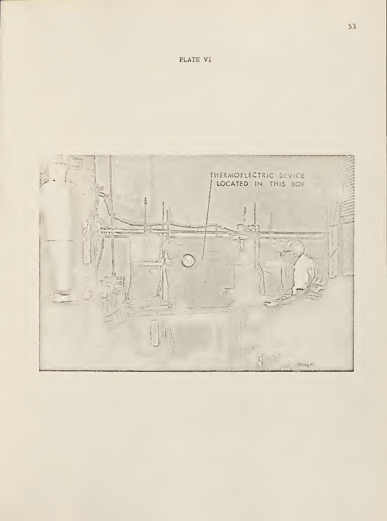
PLATE VI

THERMOELECTRIC DEVICELOCATED IN THIS BOX

/

53

\J r'j

>--*:;

'in II HI I

54

operate for 4 to 6 hours to "boil off" the air from the water. This deaer-

ated water was then removed from the vacuum tank by means of a water syphon

system and then pumped into the main supply tank for release into the water

baths. It was found that deaerated water helped to maintain a more constant

flow through the system. Air in the water can accumulate at various loca-

tions in the system particularly in the needle valves and precision flow-

raters thus causing variations in the water flow rate.

A return tank provided a method of collecting the liquid from the over-

flow tubes and the outlets from the thermoelectric device. A pump connected

to the return tank allowed the liquid to be either transferred to the vacuum

tank for deaerating or to the main supply tank for return to the water

baths. A high quality water filter was installed after the water pump to

further assure clean water for the system.

A 500-gram precision scale provide for accurate batch weighing of 300

gram samples of the liquid flowing through each circuit. Electric solonoid

valves provided for selection of the liquid from each flow circuit for batch

weighing. A sample was taken each time temperature and power data were

noted. Any change in flow rate was thus quickly ascertained and corrected.

Precision flowrators were used to determine the approximate rate of

flow through each circuit. However final determination of the flow rate

was made with the precision scale.

A diagram of the temperature measurement instrumentation is shown in

Plate VII. Temperatures were measured using calibrated copper-constantan

thermocouples connected to a high quality thermocouple switch. The output

terminals on this switch were connected to the input terminals of an elec-

tronic ice bath. The electronic ice bath provided a highly stable reference

EXPLANATION OF PLATE VII

Diagram of temperature measurement instrumentation.

56

Zo<

LU O

o oTV+ I

0990

UJ_Jo_

oOo01UJXH

X

X

I— W>

QCL "-»

Q i±:

Z

UJ

O

zUJ

oa.

x<1

/"

<3

57

junction for the measurement system without the need for inaccurate water

type ice baths. The output from the electronic ice bath provided a precise

millivolt signal that could be accurately measured by a precision potenti-

ometer. The supply voltage to the electronic ice bath was precisely

regulated to further assure accurate reference junction output.

The difference between the inlet and outlet water temperatures was

determined by connecting the inlet and outlet thermocouples so as to buck

each other. This connection was provided at the thermocouple switch by

connecting the constantan terminals together with a short length of constan-

tan wire. The output from these thermocouples was then connected to a

double pole-double throw knife switch and thence to the input terminals

on the potentiometer. When it was desired to measure the temperature dif-

ference the thermocouple switch was placed in position zero (all contacts

open). The knife switch could then be positioned so as to measure the

temperature difference. The electronic ice bath is not connected into the

measurement circuit during measurement of the temperature difference,

because of the open contacts in the thermocouple switch.

Plate VIII is a diagram of the direct current power supply for the

thermoelectric module and the electrical measurement instrumentation. The

direct current power for the thermoelectric module was obtained from two

6-volt automotive type lead acid batteries connected in parallel. Two

rheostats were connected in parallel and inserted in one of the power lines

to the module. One rheostat was used to control the largest portion of the

voltage drop to the module from the batteries. The second rheostat was used

to drop a small portion of the voltage and acted as a fine adjustment for

the current to the module. By this means the current to the module could

EXPLANATION OF PLATE VIII

Diagram of direct current power supply for thermoelectric module

and electrical instrumentation.

59

H

FINE ADJUST

RHEOSTAT

COARSE ADJUST

RHEOSTAT

'

5 >-

o £

* <CO 1

O

y

DC AMMETER

/

Q 2> h-

_/

DCVOLTMETER

ULU lu

LL

c:>

02LL

I

I•

1

;

!

i

>LU

60

be precisely controlled.

A direct current ammeter and voltmeter were used to measure the power

to the module. The ammeter had a full range of 15 amperes and the voltmeter

a full scale range of one volt. The voltmeter could be read to .005 volts.

EXPERIMENTAL DATA

Analysis of Laboratory Data

The laboratory data were programmed for multiple-regression analysis

by an IBM 1410 computer. Plates IX and X graphically show the laboratory

data along with the theoretical data. Appendix C shows the data furnished

the IBM 1410 computer.

The following equations were used for the statistical analysis:

1. 77" = a + b^ + cT3

2. 7Fl

= a + B7T2

+ c7T3

+ d^27"3

3. 7Tl

= A + B 7T2

+ C 7T3

+ D 7T2T3

+ E 7T3

4. 7Tl

= A + B 7T2

+ c 7"3

+ D 7]3

2

The data were also converted to natural logarithmic values. These

values were also processed by the IBM 1410 computer for the best fit analy-

sis of an equation of the form;

log 7Tl

= A + Blog 7T2

+ Clog 7T3

(82)

from equation (82) an equation of exponential form can be derived

as follows;

Tx= *

A<>7

2

B) (7T

3

C) (83)

EXPLANATION OF PLATE IX

Plot of theoretical and laboratory data of the pi term Q /P on

the pi term(T ,. -T . )/At while holding the pi term W /W, constantr wih wic c c c h

and the pi terra T . /At constant at selected values,wic c

62

x:

Cm

o 00 K *o 10 "*. CO CNo o O o c> o o c>

ooT

^Ma/ Dc i*JL)

EXPLANATION OF PLATE X

Plot of theoretical and laboratory data of the pi term Q /P , onJ r x wb

the pi term W /W, while holding the pi term(T . , -T . )/At constantr c h r \ W1 h W1C c

and the pi term T . /At constant at selected values.r W1C c

64

04

qM</

:d/ D(50

65

From the multiple regression analysis by the IBM 1410 computer the

following polynomial equation was determined to provide adequate precision

for engineering design;

7fl

= 1.18418 - 0.02457 W2

- 0.05885^~

3(84)

(R2

= 0.859 , > = 0.02693)yx

The exponential equation obtained from the computer was as follows;

T1

= 2.094! ( 7T2

)-°- 37515 (7r3

,-°-°"66(85 )

(R2

= 0.874 , A> = 0.03015)y«x

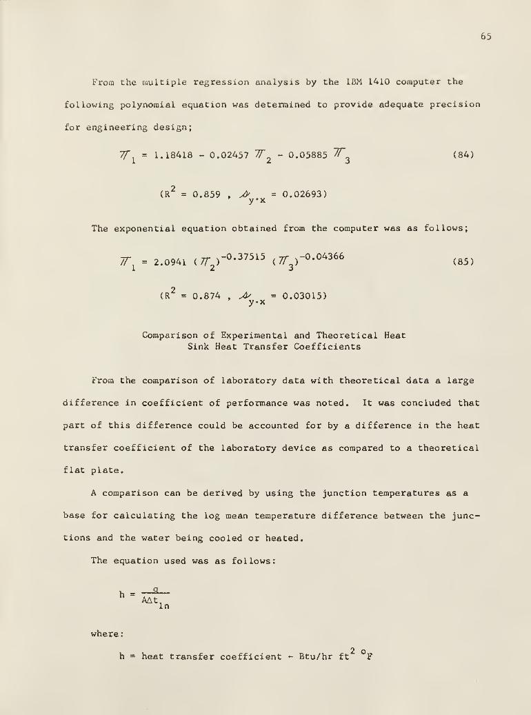
Comparison of Experimental and Theoretical HeatSink Heat Transfer Coefficients

From the comparison of laboratory data with theoretical data a large

difference in coefficient of performance was noted. It was concluded that

part of this difference could be accounted for by a difference in the heat

transfer coefficient of the laboratory device as compared to a theoretical

flat plate.

A comparison can be derived by using the junction temperatures as a

base for calculating the log mean temperature difference between the junc-

tions and the water being cooled or heated.

The equation used was as follows:

h = -a-AAt.

In

where

h = heat transfer coefficient - Btu/hr ft F

66

At

2A = area of heat transfer surface - ft

q = rate of heat transfer - Btu/hr

AtIn t .

- t.

lnt - tWO J

and:

t .= inlet water temperature - F

ot = outlet water temperature - Fwo r

t. = junction temperature - F

The calculated heat transfer coefficients are shown in Tables 2 and 3.

Also shown are the ratio between the experimental values and the theoretical

values. From this data it was concluded that the heat transfer coefficient

of the experimental device was greater than the coefficient for a theoretical

flat plate under the assumed conditions. The ratio of the experimental to

the theoretical heat transfer coefficient related to the cold and hot junc-

tions was about 3.32:1 and 2.46:1, respectively.

DISCUSSION

The results of this research indicate that the methods and equipment

used to conduct the laboratory tests were adequate to determine dimension-

less term relationships for engineering design requirements. A device hav-

ing larger capacity for cooling could improve on the accuracy of laboratory

measurements by providing a greater temperature drop as the liquid passes

through the heat exchanger. Also the flow rates could then be increased by

providing adequate systems for handling the flow of liquid and for liquid

bath heating and/or cooling.

67

Ea)

oAJ

-o

cd)1-1

o•H*w

oou1-1

a;iaj.

(0

c«

AJ

0)

c

00c

oo

CM

a)•—<

H

waj

*4-l CO 0)

o o

(0 m-i

as -

H Oi-i a)

£

ajc0)

H-l

<A-I

a)

o

u<uU-l

caj

H

a)

33

Cma-> O

s-

33

34-1

ca

CMF-l AJa] «4-4

u.

u33u

0}

a. dx ajW CQ

c-i Cm

aj O<3

O CM

H Cm

A °

CO •

aj g CmO (0 OC H3»->

a>AJ U-l

0} wa) cx <o

Wi

H3AJCQ

(0 •

0) O

m oo-• o

m

o

oooo

CO CO

oo00

co co vOom o

-JCOm o CO

CM

COCOCOCOCOCOCOCOCOCOmCO

oCO

CO

mcr>inooco\A5CM«-*mcM m~* CMm m

on O -•m m oo on co *->

mm onm nO

ONmo m o

m00

00 \£>

on

ON

co co 00 00 00 00 00vO

oo 00

onCM

oo

mco

O o o> oon on r^ co

o o o Or» r» r» r-»

o o o or-> r» oo oo

o< a. o o O O o o O£ O Cm • • • • • « •

u U o CM CM CM CM CM CM CMH O

o o o o o• • • • •

CM CM CM CM CM

o>mcoooocoooN»3'ON'^cM• •••••••••••O O '-* -H •—i-h.—(.—<»^OCM—<cocor^r^vovovovovosor^r^

0)

-auou<y

t-i

w0)

3AJ<3

>-

CJ

Q.s

co00

oON

vO

CO

oo oo 00 CM CO oo

AJuc3i-l CM

r^r^

co cm

~* COm m

vOON

00

00GO

OON

ooo

coONco CO CO

inCO co co

CMCO

-3"

CO CO COvOCO

oco co

-H CM CO m vo 00 ON O -* CM CO m

CMCO

CO

m

CO -H r^ >* CO ON ON CO r^ —> ^* ON >J CM <r

p̂^CM o

coNO CO vO

M3 vOONm o ON o ON

09

0)

00(0

u0)

><

68

CUS-J

3+-»

CO

Ucu

a.e0)uco•HUoc3

oX

T3CU

0)

ccu

•HCJ

•i-l

vw

0)

(J

>j

cu<4-J

CO

cCO

S-i

uuCO

(1)

jr

.*c

00c

<3

0)

33

CO

a).—

i

JO0}

H

iwO

o o•H -H4-J U-4

CO M-l

oo

i—

i

cO

CO U

C 4JO CU

S U•h oM CU

CU XO.HXW o

c

•Hu

•f-l

U-l

IWcu

oc_>

>-i

a>

CO

ccO

MH

cO

0)

o•H4-1

a

O0)

-CH

CN4-J

CM

r-l

n3

CO

CN

cCU

S•r-l

UCU

Cu

uCM

(£4

J-1

S3

34J

CQ

C

+J o<

Xo -"*

u*

£ °

a. oE w InQ) -H oH oi

c•

•H CUU E u,o a) oC H3

u

J-> C4-I

cO iQ

a; c33 co

uH

03

3P

J-J

CO •

cu o

o nO co vO o oo o r» 00 00 <r CMm CM o r» 00 m r^ CO >r on f—i >*

CNCNCOCMCMCNCNCNCN.-HCNCN

00-^C00000O>*LnO<fC0nO

COr-l

f-4

oo

00CN

m

ooo

oo

CO CM

CO CO

vOCN

CN

m

•<rm onnO

ONCO

CO nO CO oo

cn <t^ o

on

asas

cno

oo

COcx>

oo>

CNON

oON

CNON

oON

CNo

oo

ONoON

r-» cn

NO ON-H CN

CN CN

CO

O -•oo 00

r-l COCM

<—

i

ONnOCN

ONvO

00CO

ONoo

CNr-l

CNCN

ooNO as vO

CMON

NO m m >* in vf CM <t <f r^ «n CO m >r

1—

1

i—

*

r-

1

NO CN CN o —4 r^ 00 o o ON CM

vo oo oo

CNON

00 -vT

00 ~*

CM NO CN CM O <—l —4 O CN• • • • • • • • •

>r CN CO CN CN CM CN CN CN

oo

CN

vO CO in CO CM ON CO

oo m r-.

i—I r-t Omo

m mo ~* o o

-< m

xicu

•auoV0)i-l

CO

CU

u34-J

cO

CU

cuEcu4-t

CO NOCN —i

,-< <r

CN ~4• •

CN CN

m r*

ooCO

oCO

ON ON 00 CN CM CM CM

O•H•U

Oc3

ON 00

CN co CNnO

^ o ONNO

CN oz CO m

•-• cn co ^ in no oo ON <-* cm co •* m

vO

CM

vO

CN

<r ON <f •J- >o- cm ON CO -3- r-* ON CO r- »-* <r

NOooo NO

CMON nO

oooo

NOo

COoo

CNNO

ON00

CN NOoo

CO

CU

00cO

ucu

><

69

Multiple regression was used to determine the relationships between the

pi terms involved in the analysis. Polynomial equations of the form

77 = A + B 77 + C 71 and exponential equations of the form 77 = C 7f 77

were developed from computer programs. The equation showing adequate fit to

the data and having the least number of terms was chosen from the group of

equations solved by the computer programs.

As shown in Plate IX the relationship of 77".( Qc / Pwb ) to 7"

(Twih-Twic/Atc) was almost linear with 7T (Wc/Wh) held constant. Plate X

shows a non-linear relationship of 7T (Qc/Pwb) to 77 (Wc/Wh) with

77« (Twih-Twic/Atc) held constant. The above relationships were approxi-

mately true for both theoretical and experimental data.

The mercury thermoregulators used to maintain constant water bath

temperatures were very sensitive. Difficulty was experienced when mounting

these regulators directly on the sides of the water baths. The slightest

vibration from the stirrer motors could cause the regulator relay to

chatter. The final solution to this problem was to mount the regulators

on a rod which was isolated from the water baths.

CONCLUSIONS

The following conclusions were drawn from the analysis and data

presented

:

1. The method of dimensional analysis can be used to determine the

operating characteristics of a thermoelectric heating/cooling device. The

device can be either operated with liquid or air flowing through the heat

sinks or liquid through one sink and air through the other. For example the

device could be used to cool and heat water or cool water and heat air.

70

2. The slopes of the graphs for the experimental and theoretical data

were not exactly the same. It is believed that experimental error can

account for part of this inaccuracy. The experimental data showed that for

77* Twi h — Twi c ~tt Wc //*

//„( 7"7 ) constant, // „ (~) decreased in value as '/ . (cooling CO. P.)2 Ate 3 Wh 1

°

increased in value and appeared to be a curvilinear function. Also when

''^(777) was held constant, f/ n ( 77 ) decreased as 7T. (cooling CO. P.)3 Wh 2 Ate 1

increased and the relationship was essentially linear. Both relationships

were in general agreement with the predicted functions as derived from the

theoretical analysis.

3. Another factor which could have caused a deviation between experi-

mental and theoretical results could be a difference in the heat transfer

coefficient of the experimental device. The theoretical calculations were

based on an emperical equation for a flat plate under laminar flow condi-

tions. Although the experimental device approached a flat plate configura-

tion, the liquids entered and left the heat transfer system at right angles.

This could have caused entrance and exit effects that the theoretical

analysis did not include.

4. The experimental data did not show any measurable difference due to

different water inlet temperatures at the cooling side of the device. From

the theoretical data an error of less than 0.1 degree Fahrenheit in the

measurement of the temperature drop of the water being cooled could have

nullified the theoretical difference due to the inlet water temperature.

Since the inlet water temperature appeared to have no significant effect,

Twicthe fourth Pi term (—-— ) was eliminated from the statistical analysis of

the experimental data.

5. An empirical equation for the type of heat sinks used in this

71

research was not available. Therefore close agreement between actual values

of experimental and theoretical data could not be expected.

SUGGESTIONS FOR FURTHER RESEARCH

Laboratory experiments of the type described here, require highly

accurate instruments. Instruments for measuring the electrical power deliv-

ered to the device should be as accurate as possible. Thermocouples for

determining the temperature drop of the liquid being cooled should be

calibrated.

It was possible with the instruments available and calibrated thermo-

couples to measure a temperature change of 2 F in the liquid being cooled.

In future research a larger device should be assembled so as to provide a

greater heat transfer capacity. This greater heat transfer capacity would

result in a greater temperature drop of the liquid being cooled. The result

should be a greater degree of precision in the measurement of the temperature

drop of the liquid.

Other investigators who may perform similar research should carefully

consider the precise control of liquid flow, and assure themselves of reli-

able equipment. A closed system for the liquid circulation with suitable

filters should be considered for future research. However the open type

system and filters used in these tests proved to be satisfactory.

Future research should be carried out with other temperature drops of

the liquid being cooled. The tests reported were performed for the liquid

being cooled 2 F. Additional research would provide a family of equations

related to various temperature drops. Such equations could then be applied

to engineering design for a particular device.

72

Also these tests were performed with a current flow of 15 amperes.

Future tests should be conducted on a device with other currents, i.e. 20,

25, and 30 amperes, or up to the limit of current for the particular thermo-

electric module being used.

Future research should encompass the preliminary testing of a particu-

lar device to determine the heat transfer coefficient of the heat sinks, if

a satisfactory theoretical heat transfer coefficient is not available.

73

ACKNOWLEDGMENTS

The author owes much to his wife Jean and sons Jim and Bob, for their

patience, cooperation and loving support for his work. They must have felt

at times, that they did not have a husband or a father.

Many thanks are expressed to Dr. Truman E. Hienton, Chief, Farm Elec-

trification Research Branch, Agricultural Research Service, U.S. Department

of Agriculture, for his wisdom and patience. Largely due to his persuasion

the author accepted the challenge and opportunity to do advanced work. His

kindness and consideration are much appreciated.

Grateful acknowledgment is expressed for my advisors who contributed

with their support, guidance and thoughtfulness. Thanks to Dr. George H.

Larson, Head, Agricultural Engineering Department and Dr. Teddy 0. Hodges

and Professor Ralph I. Lipper of the Agricultural Engineering Department.

The author appreciates very much the inspiration and guidance rendered to

him by Professor Wilson Tripp, Mechanical Engineering Department.

The author also wishes to thank Herbert D. Ball, Mechanical Engineering

Department for his interest and helpful advice, Dr. Arlin H. Feyerherm,

Department of Statistics, for his guidance, Professor Michael H. Miller,

Mathematics Department and Computing Center, for his guidance in programming

the IBM 1410 computer, Dr. Jacob J. Smaltz, Industrial Engineering Depart-

ment, for instruction and guidance in the use of the IBM 1620 computer.

The understanding, helpfulness and moral support received from the late

Chester Paul Davis, Jr., are also acknowledged.

The high quality of the thermoelectric modules and accessories supplied

by Frigistors Ltd., Montreal, Canada are appreciated. Also the author

acknowledges the use of Frigistor module performance characteristics as

74

part of the theoretical analysis.

And to the friends who were concerned and contributed with their moral

support, the author expresses deep appreciation and thanks.

And last but not least, to my mother the author gives many thanks for

all her sacrifices. She advised the author to accept this opportunity when

she knew that it would separate our family at a time when she had hoped we

would be near to them.

75

BIBLIOGRAPHY

Cox, E. F.

Research on Thermoelectric Heat Pumps. Research and DevelopmentProgress Report No. 79. United States Department of the Interior,November, 1963.

Davisson, J. W. , and Joseph Pasternak.Status Report on Thermoelectricity. Naval Research LaboratoryMemorandum Report No. 1404. March, 1963.

3.

4.

Davisson, J. W. , and Joseph Pasternak.Status Report on Thermoelectricity.Report No. 1361. January, 1963.

Naval Research Laboratory

Davisson, J. W. , and Joseph Pasternak.Status Report on Thermoelectricity. Naval Research LaboratoryMemorandum Report No. 1361. October, 1962.

5. Davisson, J. W. , and Joseph Pasternak.Status Report on Thermoelectricity. Naval Research LaboratoryMemorandum No. 1241. January, 1962.

6. Egli, Paul H.

Thermoelectricity. John Wiley and Sons, New York, I960.

7. Feldman, Charles L. , S. F. Martin, and W. A. McConarty.Optimization of Cascaded Peltier Coolers. American Society ofHeating, Refr- ,oration and Air-Conditioning Engineers. Paperpresented January, 1965.

8. Frantti, E. W.

Design of Model of a Thermoelectric Air Conditioning System forSubmarines. Report No. 9161-01208-208(1). New Products Engineer-ing Department, Westinghouse Electric Corporation.

9. Fuller, Marvin A.

Some Aspects of Mass Production of Thermoelectric Heat PumpModules. AIEE paper No. CPA 62-5077. May, 1962.

10. Golubyatnikov, N. G.

Preservation of Milk Quality Using Semiconductors. (Russian)Termoelektrogenerator Kholoda-Nagrevatel' Vestnik Selkhos Nauki,1958 (10), 99-103.

11. Heikes, Robert R. , and Roland W. Ure, Jr.

Thermoelectricity: Science and Engineering. IntersciencePublishers, New York, 1961.

76

12. loffe, A. F.

Semiconductor Thermoelements and Thermoelectric Cooling. Info-search Ltd., London, 1957.

13. Jakob, Max, and George W. Hawkins.Elements of Heat Transfer. John Wiley and Sons, New York, 3rdEdition, 1959.

14. Miller, R. C, R. R. Heikes, and A. E. Fein.

Dependence of the Thermoelectric Figure of Merit on Energy Band-width. Journal of Applied Physics, Volume 33, No. 6, June, 1962,1928-1932.

15. Newton, Alwin B.

Thermoelectric Systems of Cooling and Heating. Heating, Pipingand Air Conditioning, October and November, 1963.

16. Pomazanov, I. N. , and P. L. Tikhomirov.Thermoelectric Refrigerator Operating on Heat Energy.Kholodilnaya Tekhnika, Volume 4, 1961, 24-27.

17. Pritchard, W. Maurice.The Coefficient of Performance of Thermoelectric Cooling Devices.Proceedings of the IEEE, April, 1964, 442-443.

18. Rajic, Rajica.Refrigeration Techniques and Thermoelectric Phenomena.Referativnyy Zhurnal, Metallurgiya, No. 8, 1962.

19. Siegla, D. C. , and J. B. Chaddock.Heat Transfer Analysis of a Thermoelectric Module for Refrigera-tion. ASHRAE Paper presented in January, 1965.

20. Stoecker, W. F. , and J. B. Chaddock.Transient Performance of a Thermoelectric Refrigerator UnderStep-Current Control. ASHRAE paper presented in June, 1963.

21. Ure, Roland W. , Jr.

Comments on Thermal Conductivity in Two-Phase Alloys. Journalof Applied Physics, Vol. 33, No. 7, July, 1962, 2290-2292.

22. Progress Reports 1 through 5. Thermoelectric Air ConditioningSystems for Submarines. Bureau of Ships, April - May, 1959.

23. Report No. 1. Phase II. Thermoelectric Air Conditioning Systemsfor Submarines. Bureau of Ships, November - December, 1959.

24. Design a Specific Prototype, Including Controls, of a ThermoelectricRefrigerating System for Use Aboard Submarines. Final ReportPhase II, Bureau of Ships, November 25, I960.

77

25. Submarine Food Storage Project, Phase I Report, Borg-Warner Corpora-tion, September 1, I960.

26. Design Study to Optimize the Application of Thermoelectric Materialsfor Refrigerated Spaces Aboard Submarines. Bureau of Ships,

Final Report, Phase I, December, 1959.

78

APPENDIX A

Determination of Conversion Factor to Convert

Thermal Conductivity from Metric Units to

British Thermal Units

79

Determination of conversion factor to convert from gram calories per

square centimeter per degree Centigrade per second/centimeter to British

Thermal Units per square foot per degree Fahrenheit per hour/foot.

-3Gram calories x 3.968 x 10 " = British Thermal Units

Degrees Centigrade x 1.8 = degrees Fahrenheit

-3Square centimeters x 1.076 x 10 = square feet

Centimeters30.48

= feet

Secondsl6bT~

= hours

and;

gm. cal.k =

2 °^ /sec. cm. C./cm.

Substitution of these conversion units in the above equation results in the

following relationship;

k _ (gm. cal.)(3.9681)(10~3

)

(

OC.)(1.8)(cm.

2)(1.076)(10"3 )

(

^^:) /^a7^3600 30.48

k = (3.968)(3600)(1.8)(1.076)(30.48)

Btu.k = 241.97

hr. ft.2°F./ft.

Therefore:

B|u^m

gm^cj^(241>97)

hr. ft. F./ft. sec. cm. C./cm.

80

APPENDIX B

Sintered Frigistor Performance Data

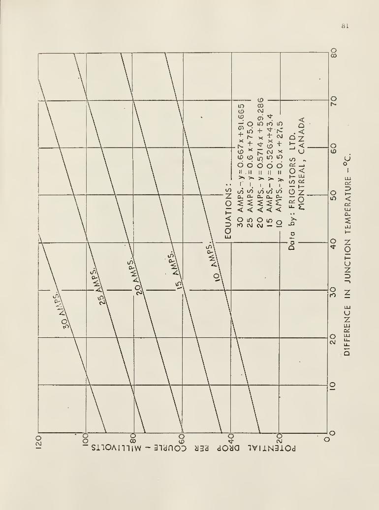
81

intoCO

COCOC\J

oS

oCO

- O in ro in o£*> »- 2 < . <* 4- ^ * 4-N 3 <" CD + ^ <CD

x|^ CVJ x <j

CD cD in in m to „

b d d 6 d c^ _i

ii. ii ii n ii o<

^ >» >» =•* >»l— UJtO C£

• i.i i i

t— h-

t/) io to «/> to o zo_ a- a. o_ c-

S oZZ £:>£< < < < <O in O in oro c\J cvj — ^

• aQ

O

OCD

Om

uo

<UJa.

3

2 zoi—uz3

IO ±

uzUJ

O i"

^ it

"o cr oO CO <x>" snoAimw - 3idnoD

oH3d dOya 1VIJLN3iOd

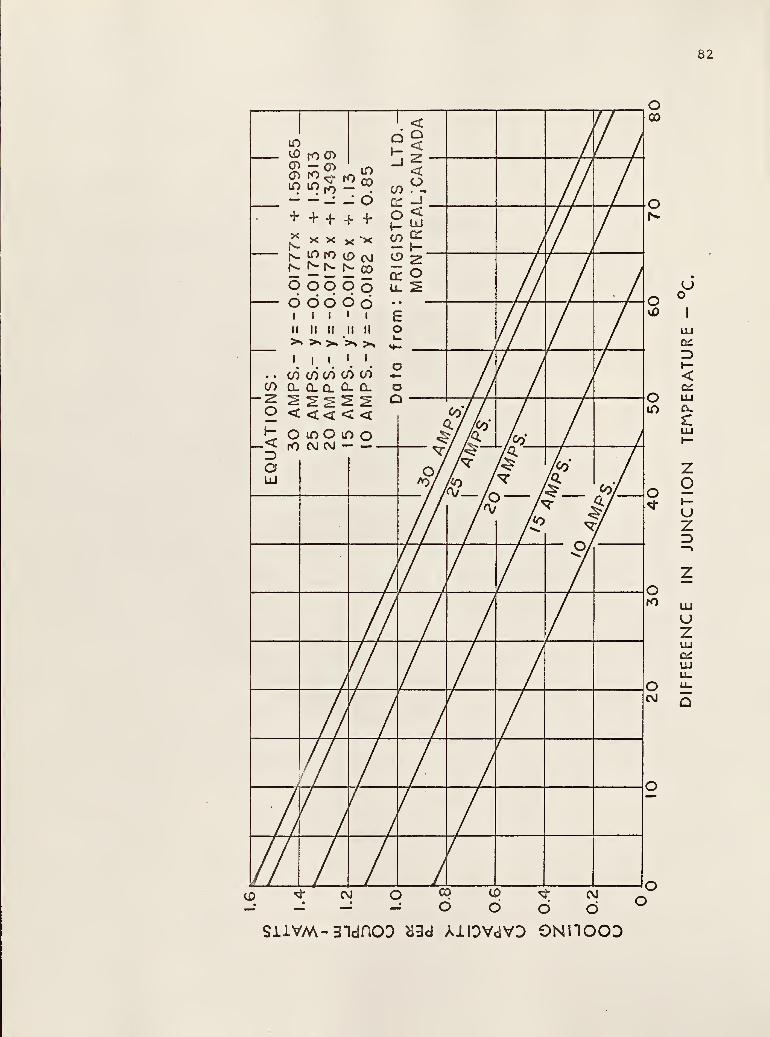
82

o

ID

<LU

LU

zo»—

uz3

LU

zLU

LU

SHVM-31dnOD tf3d AlDVdVD ONHOOD

83

APPENDIX C

Data Programmed for Multiple-regression

Analysis by IBM 1410 Computer

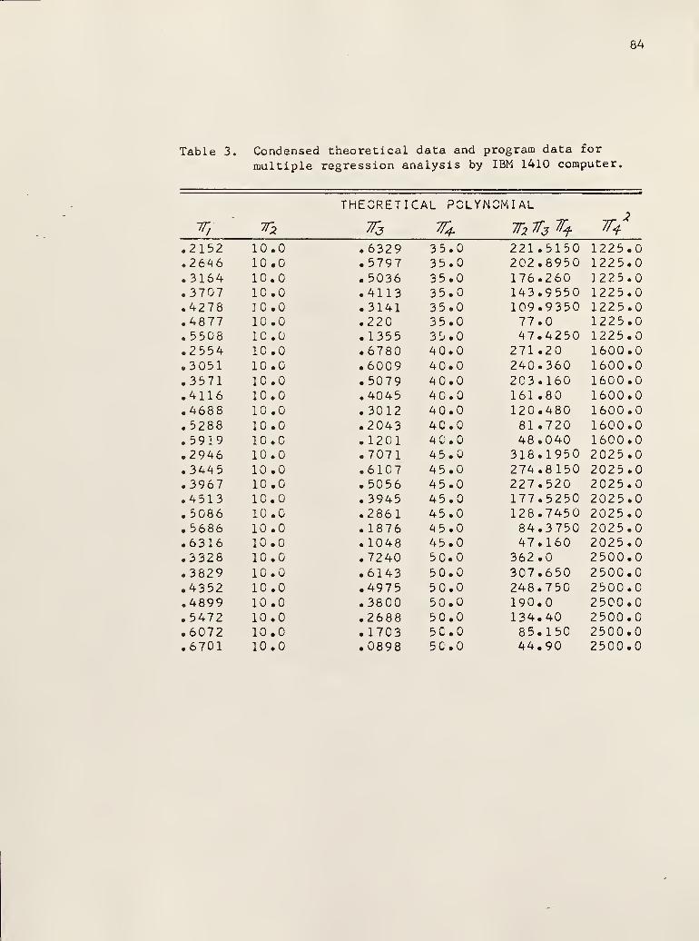
84

Table 3. Condensed theoretical data and program data for

multiple regression analysis by IBM 1410 computer,

THEORETICAL POLYNOMIAL

.2152 10.0

.2646 10.0

.3164 10.0

.3707 10.0

.4278 10.0

.4877 10.0

.5508 10.0

.2554 10.0

.3051 10.0

.3571 10.0

.4116 10.0

.4688 10.0

.5288 10.0

.5919 10.

c

.2946 10.0

.3445 10.0

.3967 10.0

.4513 10.0

.5086 10.0

.5686 10.0

.6316 10.0

.3328 10.0

.3829 10.0

.4352 10.0

.4899 10.0

.5472 10.0

.6072 10.0

.6701 10.0

.6329 35.0

.5797 35.0

.5036 35.0

.4113 35.0

.3141 35.0

.220 35.0

.1355 3^.0

.6780 40.0

.6009 40.0

.5079 40.0

.4045 40.

.3012 40.0

.2043 40.0

.12 01 40.0

.7071 45.0

.6107 45.0

.5056 45.0

.3945 45.0

.2861 45.0

.1876 45.0

.1048 45.0

.7240 50.0

.6143 50.0

.4975 50.0

.3800 50.0

.2688 50.0

.1703 50.0

.0898 5 0.0

221..5150 1225 .0

202,,8950 1225 .0

176 .260 1225 .0

143,.9550 1225 .0

109 .9350 1225 .0

77,.0 1225 .0

47,.4250 1225 .0

271 .20 1600 .0

240 .360 1600 .0

203 .160 1600 .0

161 ,80 1600 .0

120 .480 1600 .0

81 .720 1600 .0

48,.040 1600 .0

318,,1950 2025 .0

274 .8150 2025 .0

227 .520 2025 .0

177 .5250 2025 .0

128,,7450 2025 ,0

84 .3750 2025 ,0

47,,160 2025 ,0

362,.0 2500 ,0

307,,650 2500 .0

248,,750 2500 ,0

190,.0 2500,.0134,,40 2500,,085,,150 2500,.044,.90 2500,,0

Table 3 (cont. ).

85

THEORETICAL PCLYN CM I A L

**r, Ts 7% 7T4 T2 T3 77i-

.2152 14. 1042 .50 35.0 246.8235 1225.0

.2646 12.3314 .50 35.0 215.7995 1225.0

.3164 10.1093 .50 35.0 176.912a 1225.0

.3707 7.5992 .50 35.0 132.9860 1225.0

.4278 4.8803 .50 35.0 85.4053 1225.0

.4877 2=*527 .50 35.0 35.9223 1225.0

.5 508 -0.8905 .50 35.0 - 15.5838 1225.0

.6172 - 3.9311 .50 35.0 -68.7943 1225.0

.6873 -7.0192 .50 35.0 -122.8360 1225.0

.2554 14.8612 .50 4CO 297.2240 1600.0

.3051 12.6667 .50 40.0 253.3340 1600.0

.3571 10.2022 .50 40.0 204.0440 1600.0

.4116 7.5539 .50 40.0 151.0780 1600.0

.4688 4.7470 .50 40.0 94.940 1600.0

.5288 1.8495 .50 40.0 36.990 1600.0

.5919 - 1.1205 .50 4C.0 - 22.410 1600.0

.6582 - 4. 163o .50 40.0 - 83.260 1600.0

.7281 -7.2599 .50 40.0 -145.1980 1600.0

.2946 15.1715 .50 45.0 341 .3588 2025.0• 3445 12.7526 .50 4 5.0 286.9335 2025.0.3967 10.1319 .50 45.0 227.9678 2025.0.4513 7.3707 .50 45.0 165.8408 2025.0.5086 4.5188 .50 45.0 101.6730 2025.0.5686 1.5944 .50 45.0 35.8740 2025.0.6316 - 1.4093 .50 45.0 - 31.7093 2025.0.6978 - 4.4674 .50 45.0 -100.5165 2025.0.7674 - 7.5479 .50 45.0 -169.8278 2025.0.3328 15.2394 .50 50.0 380.9850 2500.0.3829 12.6574 .50 50.0 316.4350 2500.0.4352 9.9418 .50 50.0 248.5450 2500.0.4899 7.1355 .50 50.0 178.3875 2500.0.5472 4.2249 .50 50.0 105.6225 2500.0.6072 1.2669 .50 50.0 31.6725 2500.0.6701 - 1.7206 . 50 50.0 - 43.0150 2500.0.7361 - 4.7692 .50 50.0 -119.230 2500.0.8055 - 7.8473 .50 50.0 -196.1825 2500.0

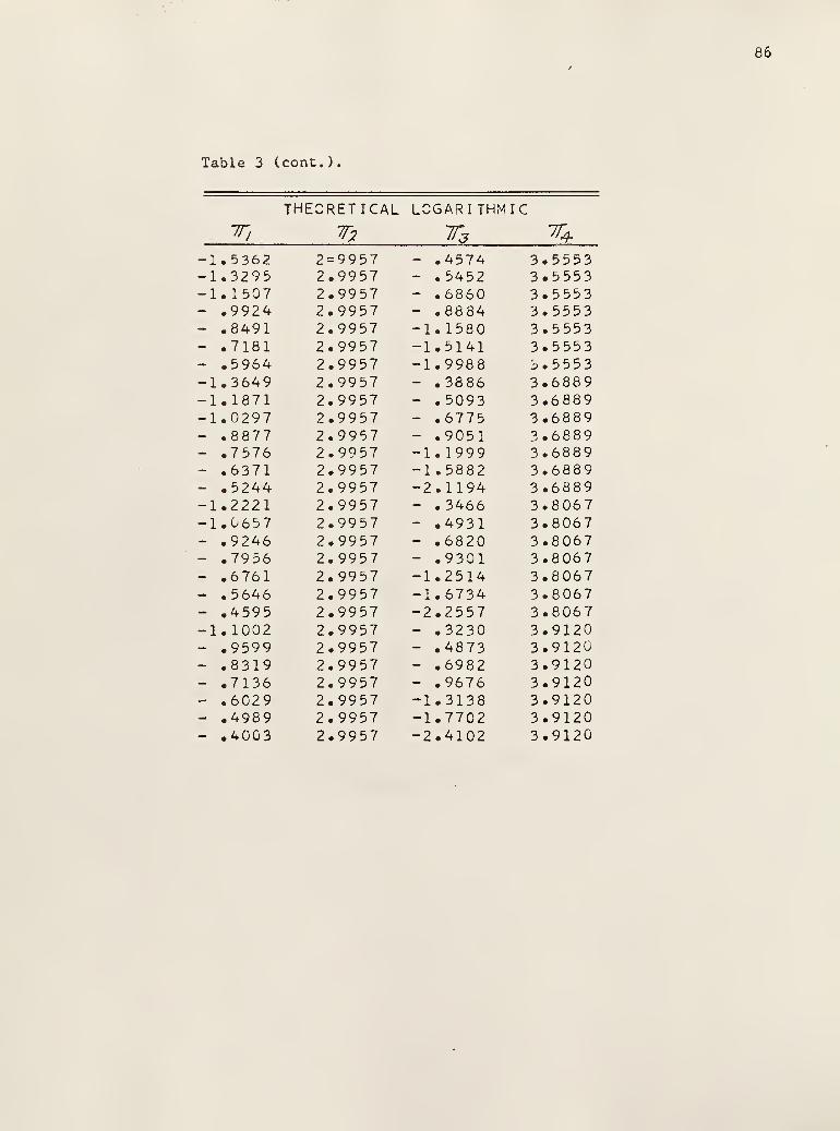
Table 3 (cont.).

86

THEORETICAL LOGARITHMIC

in T* Tj ^f .

-1.5362 2=9957 - .4574 3.5553-1.3295 2.9957 - .5452 3.5553-1.1507 2.9957 - .6860 3.5553- .9924 2.9957 - .8884 3.5553- .8491 2.9957 -1.1580 3.5553- .7181 2.9957 -1.5141 3.5553- .5964 2.9957 -1.9988 3.5553-1.3649 2.9957 - .3886 3.6889-1.1871 2.9957 - .5093 3.6889-1.0297 2.9957 - .6775 3.6889- .8877 2.9957 - .9051 3.6889- .7576 2.9957 -1. 1999 3.6889- .6371 2.9957 -1.5882 3.6889- .5244 2.9957 -2.1194 3.6889-1.2221 2.9957 - .3466 3.8067-1.0657 2.9957 - .4931 3.8067- .9246 2.9957 - .6820 3.8067- .7956 2.9957 - .9301 3.8067- .6761 2.9957 -1.2514 3.8067- .5646 2.9957 -1.6734 3.8067- .4595 2.9957 -2.2557 3.8067-1.1002 2.9957 - .3230 3.9120- .9599 2.9957 - .4873 3.912U- .8319 2.9957 - .6982 3.9120- .7136 2.9957 - .9676 3.9120- .6029 2.9957 -1.3138 3.9120- .4989 2.9957 -1.7702 3.9120- .4003 2.9957 -2.4102 3.9120

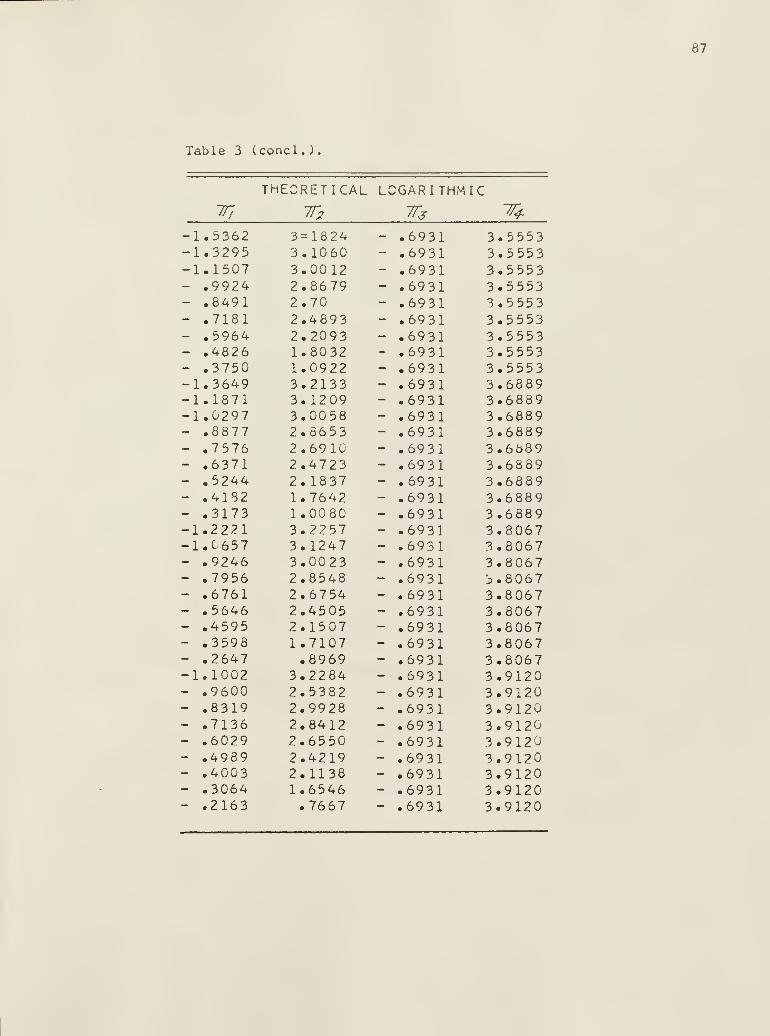
Table 3 (concl.).

87

THEORETICAL L<2GARITHMIC-ir, ir2 Tj "35

-1.5362 3=1824 - .6931 3.5553-1.3295 3.1060 - .6931 3.5553-1.1507 3.0012 - .6931 3.5553- .9924 2.8679 - .6931 3.5553- .8491 2.70 - .6931 3.5553- .7181 2.4893 - .6931 3.5553- .5964 2.2093 - .6931 3.5553- .4826 1.8032 - .6931 3.5553- .3750 1.0922 - .6931 3.5553-1.3649 3.2133 - .6931 3.6889-1.1871 3. 1209 - .6931 3.6889-1.0297 3.0058 - .6931 3.6889- .8877 2.8653 - .6931 3.6889- .7576 2.6910 - .6931 3.6889- .6371 2.4723 - .6931 3.6889- .5244 2. 1837 - .6931 3.6889- .4182 1.7642 - .6931 3.6889- .3173 1.0080 - .6931 3.6889-1.2221 3.2257 - .693] 3.8067-1.C657 3.1247 - .6931 3.8067- .9246 3.0023 - .6931 3.8067- .7956 2.8548 - .6931 3.8 06 7- .6761 2.6754 - .6931 3.8067- .5646 2.4505 - .6931 3.8067- .4595 2.1507 - .6931 3.8067- .3598 1.7107 - .6931 3.8067- .2647 .8969 - .6931 3.8067-1.1002 3.2284 - .6931 3.9120- .9600 2.5382 - .6931 3.9120- .8319 2.9928 - .6931 3.9120- .7136 2.8412 - .6931 3.9120- .6029 2.6550 - .6931 3.9120- .4989 2.4219 - .6931 3.9120- .4003 2.1138 - .6931 3.9120- .3064 1.6546 - .6931 3.9120- .2163 .7667 — .6931 3.9120

88

APPENDIX D

Condensed Laboratory Test Data

89

Table 4. Condensed laboratory data and program data for

multiple regression by IBM 1410 computer.

labcrat::ry pclync MI AL

r, Tu T3 ^2^3 ~7jZ

.9520 10.0 .5190 5.190 .2694

.9430 10.0 .5190 5.560 .3091

.9290 10.0 .6560 6.560 .4303

.9270 10.0 .5510 5.510 .3036

.8890 10.0 .7810 7.810 .6099

.8760 10.0 .7860 7.860 .6178

.8740 10.0 1.040 10.40 1.0816

.8880 9.40 .4990 4.690 .2490

.8740 10.0 .4990 4.990 .2490

.8560 11.30 .5010 5.6613 .2510

.8470 12.10 .4990 6.0379 .2490

.7810 14.30 .50 7.150 .250

.7810 15.90 .5090 8.0931 .2591

.780 15.0 .50 7.50 .250

.7340 17.40 .5020 8.7348 .2520

LABORATORY LOGARITHMIC

.0492 2.3026 - .6559

.0587 2.3026 - .5870

.0736 2.3026 - .4216

.0758 2.3026 - .5960

.1177 2.3026 - .2472

.1324 2.3026 - .2408

.1347 2.3026 - .0392

.1188 2.2407 - .6951

.1347 2.3026 - .6951

.1555 2.4248 - .6911

.1661 2.4932 - .6951

.2472 2.6603 - .6931

.2472 2.7663 - .6753

.2485 2.7081 - .6931

.3C92 2.8565 - .6892

90

APPENDIX E

IBM 1620 Computer FORGO Programs

Used For Theoretical Dimensional Analysis

91

FORGO PROGRAM FORT.O SOLVE FOR PI3 H!

IBM 1620 COMPUTER:LD1NG PI2 CONSTANT

1920

10221

71

70

61

6063

6265

6468

67

TWIDELP4 =

P2 =

A = .

T W I

DC =

wc=oc=OCTTWOTPCRl =

R2 =

R3 =

DTLHl =

Yl =

IF(

°RI,-OR

CONIF(TPCGOCONIF(

TPCGOIF(TPCGOIF(TPCGOIF(

TPCGOCONDELFTCCTCDHCCTHVM =

MO WRYC = 80.TC = 2.TWIC/DELTC10,0273H=(P2) *(DELTC)+TWIC15.8.

WC*DELTC=(QC)/((12.)*<3.413))C=TWIC-DELTC=TWOC-.l(WC)**.4997(TWIC-TPC)/(TW0C-TPC)L0G(R2 )

NC=(DELTC)/(R3 )

(QC)/( A*DTLNC)( ( .0383 )*( TPC+DTLNO+9. 1325 )*(R1 )

SENSE SWITCH 1 )20,21NT 102,TPC»H1»Y1MAT(3F10.4)TINUE(ABS(Hl-Yl) ) -5C ) 7 0,70,71=TPC-1.TO 9

TINUE(ABS(H1-Y1 ))-2 0.) 60,60,61=TPC-.5TO 9

(ABMH1-Y1) )-3.)62,62,63=TPC-.lTO 9

(ABS(H1-Y1 ) )-l.)64,64,65=TPC-.-5TO 9

(ABS(Hl-Yl) )-. 5)67,67, 68=TPC-.01TO 9

TINUECG=(QC )/( 17.46)=TPC-DELCG={ (5. ) /(9. ) )*(FTC-32.

)

= (1.13+( .00678*CTC)-QCT) / ( .0176 )

=DHC+CTC•526*DHC+43.4

92

PW=( (VM+.017*DC*CTC)*( 12.*DC) )/( 10 00.

)

PWB=(PW)*{ 3.413)FTH=( (9.) /(5. ) )*(CTH)+32.QH=QC+PWBDELHG=(QH)/( 17.46)TPH=FTH-DELHGWH=.l

5 R4= (WH)**.4997DELTH=(QH)/(WH)TWCH=TWIH+DELTHIF(TW0H-TPH)6»4,4

4 WH=WH+1.GO TO 5

6 CONTINUER5 = (TWIH-TPH)/(TWCH-TPH)R6=L0G(R5 )

H2=( (WH)*(R6 ) )/( .0273)Y2=( ( .0383 )*( TPH- ( DEL TH)/(R6) )+9.132 5)#R4

18 IF(SENSE SWITCH 2)15*1015 PRINT 101,WH,H2,Y2

101 FORMAT(3F10.4)10 CONTINUE

IF( (ABS(H2-Y2) )-5 0. ) 52,52,5353 WH=WH+2.

GO TO 5

52 IF( (ABS(H2-Y2) )-20. ) 22,22,232 3 WH=WH+1.

GO TO 5

22 IF( (ABS(H2-Y2) )-3. )27,27,2929 WH=WH+.5

GO TO 5

27 IF( (ABSCH2-Y2) )-l.) 16,16,1717 WH=WH+.l

GO TO 5

16 IF( (ABS(H2-Y2) ) -. 5 ) 24 ,24 ,2525 WH=WH+.05

GO TO 5

24 CONTINUEP]=(OC)/(PWB )

P2=(TWIH-TWIC)/(DELTC)P3= (WC) /( WH)PUNCH 28,DHC,FTC,PW,DELTC,DELTHPUNCH 28, PI ,P2,P3,TWIC,TWIHPUNCH 28,WH,WC,QC,QH,PWBPUNCH 28,TPC,TPH,FTH,P4,DC

28 F0RMAT(5F10.4)WC=WC+1.GO TO 3

END

93

FCRGC PROGRAM FOR IBM 1620 COMPUTERTO SOLVE FOR PI2 HOLDING PI 3 CONSTANT

192010221

71

70

61

6063

6265

6467

66

MOWRYC =80.TC = 2.TWIC/DELTC027315..5

TWIDELP4 =

A = .

DC =

P3 =

WC =

QC =

OCTTWOTPCRl =

R2 =

R3 =

DTLHl =

Yl =

IF(PRIFORCONIF(TPCGO TO 9

CON

WC*D= (0CC = TW= TWO(WC)( TWILOG(NC=((QC)( ( .0SENSNT 1

MAT(TINU(ABS= TPC

IF(TPCGOIF<TPC

TINU(ABS= TPCTO 9

(ABS= TPC

GO TO 9

ELTC) /( ( 12. )*(3.413) )

IC-DELTCC-.l**.4997C-TPC)/ (TWOC-TPC)R2)DELTC)/(R3 )

/( A*DTLNC)3 83)*(TPC+DTLNC)+9.1325)*(R1)E SWITCH 1)20.2102»TPC»H1»Y13F10.4)E

(Hl-Yl) )-50. )70,70,71-1.

(Hl-Yl ) )-20. ) 60,60,61-.5

(Hl-Yl) )-3. )62,62,63-.1

(Hl-Yl) )-l. )64,64,65-.05

(ABS= TPCTO 9

(ABS (Hl-Yl ))-.5)66,66,67=TPC-.Ol

IF(TPCGOIF(

TPCGO TO 9

CONTINUEDELCG=(QC)/( 17.4.6)FTC=TPC-DELCGCTC=( (5. ) /(9. ) )*(FTC-32.

)

DHC=( 1.13+( ,00678*CTC)-QCT)/( .0176)CTH=DHC+CTCVM=.526*DHC+43.4

94

1510110

53

5223

2229

2725

24

PW= ( (VMPW3=(PWFTH=( (9

QH=QC+PDELHG»<TPH=FTHWH= (WOR4=(WH)DELTH=(TWIH=TPTWCH=TWIF(TWCHTWIH=TWGO TO 5

CONTINUR5=(TWIR6=LCG(H2=( (WHY2=( ( .0

IF(SENSPRINT 1

FCRMAT(CONTINUIF( (ABSTWIH=TW

+ .

)*

• )

WBQM-D/(•**

QHH

IH-TIH

017*DC*CTC)*( 12.*DO )/ (10 00.

)

(3.413)/(5. ) )*(OH)+32.

J /( 17.46)ELHGP3).4997)/(WH)

+DELTHPH)6,4,4-1.

E

H-TR5 )

)*.{

383E S

01,3F1E

(H2IH-

PH) /(TWCH-TPH)

R6 ) )/ ( .0273))*(TPH-(DELTH)/(R6) )+9.1325)*R4WITCH 2) 15*10TWIH,H2»Y20.4)

-Y2) )-20. ) 52,52*531.

28

GC TO 5

IF( (ABSTWIH=TWGC TC 5



CCNTINUP1=(QC)P2=(TWIPUNCH 2

PUNCH 2

PUNCH 2

PUNCH 2

FCRMAT(WC=WC+1GC TC 3

END

(H2-Y2) )-3. )22,22.23IH-.5

(H2-Y2) )-l.)27»27»29IH-.l

(H2-Y2) )-. 5)24, 24*25IH-.05

E

/(PWB)H-TWIO/ (DELTC)8,DHC,FTC»PW,DELTC»DELTH8,P1,P2.P3*TWIC,TWIH8,WH»WC,QC»QH»PWB8,TPC,TPH»FTH»P4,DC5F10.4)

95

APPENDIX F

Important Thermoelectric Equations

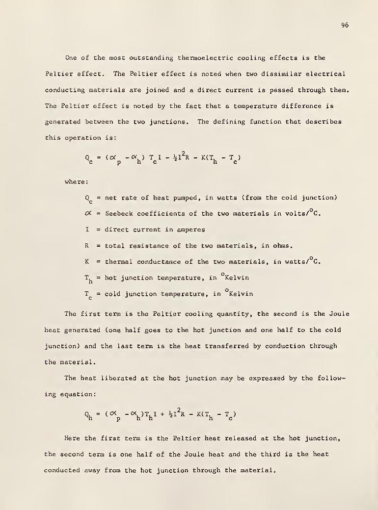
96

One of the most outstanding thermoelectric cooling effects is the

Peltier effect. The Peltier effect is noted when two dissimilar electrical

conducting materials are joined and a direct current is passed through them.

The Peltier effect is noted by the fact that a temperature difference is

generated between the two junctions. The defining function that describes

this operation is:

q =(of -Of. ) T I - %I2R - K(T, - T )

c p h c hewhere:

Q = net rate of heat pumped, in watts (from the cold junction)

OC = Seebeck coefficients of the two materials in volts/ C.

I = direct current in amperes

R = total resistance of the two materials, in ohms.

K = thermal conductance of the two materials, in watts/ C.

T, = hot junction temperature, in Kelvin

T = cold junction temperature, in Kelvin

The first term is the Peltier cooling quantity, the second is the Joule

heat generated (one half goes to the hot junction and one half to the cold

junction) and the last term is the heat transferred by conduction through

the material.

The heat liberated at the hot junction may be expressed by the follow-

ing equation:

Q = (c* -CX )T, 1 + %I2R - K(T, - T )

h p h h heHere the first term is the Peltier heat released at the hot junction,

the second term is one half of the Joule heat and the third is the heat

conducted away from the hot junction through the material.

97

A relationship has been evolved between the Seebeck coefficient, ther-

mal conductivity, and the electrical resistivity. This relationship is

expressed as a factor Z or figure of merit.

where:

S = Seebeck coefficient in volts/ C.

P = Electrical resistivity in ohm • cm.

k = Thermal conductivity in watts/cm.* C.

From this expression the dimension of Z is C

Important Formulas:

AT = i;ZT2

max. c

Q. = K(AT - AT)^1 max . max

.

AT -ATmax.

max. Z T, Th c

(c* )

2

AB

where:

AT = maximum temperature difference that can be produced by a

couple, C.

AT = operating temperature difference (T, - T ) C.

k = thermal conductivity - watts/cm* C.

T, and T = Hot and cold junction temperatures - Kelvin

98

P = Electrical resistivity - ohm-cm.

Q. = maximum cooling effect - watts.1 max

.

°

= maximum coefficient of performance for maximum cooling -max

.

dimensionless.

K = thermal conductance - watts/ C.

Z = Figure of merit

°£ = Seebeck coefficient of the materials in volts/ C.

99

APPENDIX G

List of Symbols and Explanation

LIST OF SYMBOLS USED IN THEORETICAL ANALYSIS

100

Symbol Description Units

A

C

h

I

k

L

m

Nu

Pr

Re

w

"wb

cf

cc

'hf

'he

pc

•ph

area

thermal conductance

heat transfer coefficient for flat plate

electric current (direct current)

thermal conductivity

length

mass flow rate

Nusselt number

Prandtl number

Reynolds number

electric power

electric power

rate of heat transfer

cooling capacity per couple

cooling capacity of module

heat rejected by module

thermal resistance

cold junction temperature

cold junction temperature

hot junction temperature

hot junction temperature

plate temperature on cold side

plate temperature on hot side

ft.

Btu./ft.2°F.hr.

Btu./hr.ft. F.

amperes

Btu./hr.ft.°F.

ft.

lbs./hr.

dimensionless

dimensionless

dimensionless

watts

Btu./hr.

Btu./hr.

watts

Btu./hr.

Btu./hr.

ft.2hr.°F./Btu,

°F.

°c-

°F.

°C

°F.

°F.

101

wa

Twih

Twoh

Twic

Twoc

v

V

Vm

wh

W

AtIn

At

At,

Athe

Ateg

V

e

Tl

7Tk

average water temperature

inlet water temperature on hot side

outlet water temperature on hot side

inlet water temperature on cold side

outlet water temperature on cold aide

velocity

volume rate of flow

potential drop per couple

water flow through hot junction sink

water flow through cold junction sink

water flow rate in heat transfer equation

heat transfer coefficient for flat platerelated to water flow and watertemperature

log mean temperature difference betweenplate and liquid

temperature drop of liquid due to cooling

temperature rise of liquid

temperature difference between hotand cold junctions

temperature difference across copperplate and nylon/grease separator

kinematic viscosity

density

Q /P,

c wb

(Twih-Twic)/4t

F.

'P.

'F.

F.

'P.

ft. /hr.

ft.3./sec.

millivolts

lbs ./hr.

lbs ./hr.

lbs ./hr.

Btu ./hr.ft, 2o F

w /w,c h

Twic /At

F.

°F.

°F.

°C

°F.

ft.2/hr.

lb. /ft.3

ra

dimensionless

dimensionless

dimensionless

dimensionless

102

APPENDIX H

Laboratory Test Data

103

Table 5. Bas ic laboratory test data.

Millivo Its Minutes for300 pram sample

W Wuc h

Direct currentTest No.

Twic Atc

Twih Ath

voltage

T2constant

1. 1.276 0.046 1.742 0.071 2.10 1.64 0.8301.275 0.046 1.742 0.072 2.10 1.65 0.8301.275 0.046 1.741 0.073 2.11 1.64 0.8301.276 0.047 1.742 0.072 2.10 1.64 0.830

2. 1.280 0.046 1.742 0.048 1.99 1.11 0.8251.274 0.045 1.741 0.047 1.99 1.11 0.8251.277 0.046 1.741 0.048 1.98 1.12 0.8251.276 0.046 1.742 0.048 1.99 1.11 0.825

3. 1.046 0.047 1.505 0.096 2.20 2.29 0.8051.046 0.046 1.508 0.095 2.20 2.29 0.8051.047 0.046 1.506 0.096 2.21 2.28 0.8051.046 0.047 1.506 0.096 2.20 2.29 0.805

4. 1.048 0.046 1.505 0.058 2.10 1.38 0.7951.047 0.047 1.508 0.059 2.11 1.39 0.7951.046 0.047 1.506 0.059 2.10 1.38 0.7951.047 0.047 1.508 0.060 2.10 1.38 0.795

5. 0.822 0.046 1.276 0.073 2.26 1.78 0.7850.824 0.046 1.277 0.072 2.25 1.77 0.7850.823 0.046 1.276 0.073 2.25 1.77 0.7850.823 0.045 1.277 0.072 2.26 1.77 0.785

6. 0.822 0.046 1.276 0.049 2.15 1.18 0.7800.820 0.046 1.276 0.051 2.16 1.18 0.7800.823 0.046 1.277 0.051 2.15 1.18 0.7800.823 0.045 1.276 0.050 2.15 1.18 0.780

7. 0.823 0.044 1.276 0.046 2.09 1.09 0.7750.821 0.046 1.275 0.046 2.10 1.09 0.7750.821 0.044 1.277 0.047 2.10 1.09 0.7750.822 0.046 1.276 0.046 2.10 1.09 0.775

Table 5 (cont.).

104

Test No.

Twic

Millivolts

At Twih At,

Minutes for300 gram sample

W W,

Direct currentvoltage

8.

9.

10.

11.

12,

13.

14.

15.

77~o constant

0.823 0.046 1.508 0.050 2.48 1.24 0.8000.824 0.047 1.507 0.049 2.48 1.24 0.8000.823 0.046 1.507 0.049 2.48 1.24 0.8000.823 0.046 1.508 0.050 2.48 1.24 0.800

0.824 0.046 1.336 0.048 2.32 1.17 0.7750.823 0.046 1.336 0.047 2.34 1.17 0.7750.823 0.046 1.335 0.048 2.33 1.17 0.7750.823 0.046 1.336 0.048 2.33 1.17 0.775

0.823 0.047 1.249 0.047 2.27 1.13 0.7700.824 0.046 1.248 0.046 2.26 1.14 0.7700.822 0.046 1.249 0.046 2.27 1.13 0.7700.824 0.047 1.248 0.046 2.27 1.13 0.770

1.048 0.047 1.856 0.053 2.50 1.25 0.8451.048 0.047 1.854 0.052 2.50 1.25 0.8451.047 0.048 1.855 0.052 2.51 1.25 0.8451.048 0.047 1.856 0.053 2.51 1.25 0.845

1.047 0.046 1.508 0.046 2.20 1.10 0.8051.046 0.047 1.509 0.047 2.20 1.10 0.8051.048 0.046 1.507 0.046 2.21 1.10 0.8051.047 0.046 1.508 0.046 2.20 1.10 0.805

1.046 0.047 1.710 0.048 2.42 1.21 0.8201.045 0.046 1.711 0.048 2.41 1.21 0.8201.045 0.046 1.711 0.049 2.42 1.21 0.8201.046 0.047 1.710 0.048 2.42 1.21 0.820

1.277 0.047 2.018 0.052 2.32 1.18 0.8551.276 0.046 2.019 0.051 2.31 1.18 0.8551.277 0.046 2.018 0.052 2.32 1.18 0.8551.277 0.047 2.018 0.052 2.32 1.18 0.855

1.277 0.046 1.838 0.048 2.20 1.10 0.8301.276 0.046 1.837 0.050 2.21 1.10 0.830

1.277 0.047 1.837 0.050 2.20 1.10 0.8301.276 0.047 1.838 0.049 2.20 1.10 0.830

DEVELOPMENT OF A SIMPLIFIED ENGINEERING DESIGN EQUATIONFOR A THERMOELECTRIC HEATING/ COOLING DEVICE

by

GEORGE ROBERT MOWRY

B. S., The Pennsylvania State University, 1941

AN ABSTRACT OF A MASTER'S THESIS

submitted in partial fulfillment of the

requirements for the degree

MASTER OF SCIENCE

Department of Agricultural Engineering

KANSAS STATE UNIVERSITYManhattan, Kansas

196*

The past decade has seen the development of new serai-conductor materials

which exhibit a greater thermoelectric effect than previously was available.

As a result the application of thermoelectric cooling devices may become

more feasible within the next decade or so. Devices which can cool and heat

without moving parts are already being manufactured.

The application of thermoelectric cooling may be feasible in agriculture

for such uses as milk pasturization and/or milk cooling coupled with water or

air heating or cooling.

Design of thermoelectric devices usually proceeds by selecting some

cold junction temperature to be held constant. Such may not be the case

with some applications as mentioned in this study. The development of sim-

plified engineering design equations can be of help in predicting the operat-

ing characteristics of such devices, especially if the operating conditions

are not constant. It was decided to investigate the application of the

principles of dimensional analysis to determine the relationship of the

important variables involved in a thermoelectric heating/coo ling device.

It was first necessary to explore theoretically the dimensionless Pi groups

that could be formed in order to determine the proper combination that would

yield an explicit relationship. The theoretical analysis was performed with

an IBM 1620 computer.

A simple device was fabricated to handle liquid in both heat exchangers.

The heat exchanger design approached that of a flat plate but with the liquid

entering the chambers at right angles. An empirical equation for flat plate

heat transfer was used in the theoretical analysis. Operating characteristics

of the thermoelectric module were derived from the manufacturers data.

The current was held constant at 15 amperes. The theoretical analysis

assumed water inlet temperatures on the cold side heat sink of 70, 80, 90 and

100 F. Flow rates were assumed between about 10 lbs/hr to about 50 lbs/hr.

The temperature drop of the water being cooled was assumed to be 2 F and

held constant at that value.

The data obtained from the theoretical analysis with the IBM 1620 com-

puter was programed for multiple-regression analysis with the IBM 1410 com-

puter. The multiple-regression analysis yielded an equation which showed the

mathematical relationship of the Pi groups.

Equipment was assembled in the laboratory and analysis similar to that

used with the computer program was followed. The data was then programed for

multiple-regression analysis by the IBM 1410 computer.

The results of the laboratory tests were in general agreement with the

relationships as predicted by the theoretical analysis.

development of a simplified engineering design equation ... ·...

Documents