development of an intelligent model …etd.lib.metu.edu.tr/upload/12619999/index.pdf · controller...

DEVELOPMENT OF AN INTELLIGENT MODEL PREDICTIONCONTROLLER FOR AUTONOMOUS HELICOPTERS

A THESIS SUBMITTED TOTHE GRADUATE SCHOOL OF NATURAL AND APPLIED SCIENCES

OFMIDDLE EAST TECHNICAL UNIVERSITY

BY

SEVKET ESER KUBALI

IN PARTIAL FULFILLMENT OF THE REQUIREMENTSFOR

THE DEGREE OF MASTER OF SCIENCEIN

AEROSPACE ENGINEERING

MAY 2016

Approval of the thesis:


submitted by SEVKET ESER KUBALI in partial fulfillment of the requirements forthe degree of Master of Science in Aerospace Engineering Department, MiddleEast Technical University by,

Prof. Dr. Mevlüde Gülbin Dural ÜnverDean, Graduate School of Natural and Applied Sciences

Prof. Dr. Ozan TekinalpHead of Department, Aerospace Engineering

Assoc. Prof. Dr. Ilkay YavrucukSupervisor, Aerospace Engineering Department, METU

Examining Committee Members:

Prof. Dr. Ozan TekinalpAerospace Engineering Department, METU

Assoc. Prof. Dr. Ilkay YavrucukAerospace Engineering Department, METU

Prof. Dr. M. Kemal LeblebiciogluElectrical and Electronics Engineering Department, METU

Prof. Dr. Metin U. SALAMCIMechanical Engineering Department, Gazi University

Assist. Prof. Dr. Ali Türker KutayAerospace Engineering Department, METU

Date:

I hereby declare that all information in this document has been obtained andpresented in accordance with academic rules and ethical conduct. I also declarethat, as required by these rules and conduct, I have fully cited and referenced allmaterial and results that are not original to this work.

Name, Last Name: SEVKET ESER KUBALI

Signature :

iv

ABSTRACT


Kubali, Sevket Eser

M.S., Department of Aerospace Engineering

Supervisor : Assoc. Prof. Dr. Ilkay Yavrucuk

May 2016, 81 pages

In this thesis, a new PID gain update law using linear least squares regression is intro-duced as an adaptive control method for autonomous helicopters. In addition, futureprediction analyses are conducted for error dynamics of the closed loop system usingrecursive linear least squares regression. Combining these two concepts with classi-cal PID controller, an intelligent PID controller is obtained. On the other hand, usingPID controllers, a flight controller with three control loops is developed to demon-strate the capabilities of the new intelligent controller and PID controllers of secondand third control loops of this flight controller are replaced by the newly developedintelligent controller. Thus, a new intelligent flight controller is acquired with modelprediction and adaptation abilities. Several challenging maneuvers are carried out invirtual environment for the flight controller that has no adaptation ability and the newintelligent flight controller using the same initially stable PID gains to investigate thesuccess of the new intelligent controller.

Keywords: adaptive control, pid controller, least squares regression, optimization,helicopter, simulation

v

ÖZ

OTONOM HELIKOPTERLER IÇIN AKILLI BIR MODEL TAHMINKONTROLCÜSÜ GELISTIRILMESI

Kubali, Sevket Eser

Yüksek Lisans, Havacılık ve Uzay Mühendisligi Bölümü

Tez Yöneticisi : Doç. Dr. Ilkay Yavrucuk

Mayıs 2016 , 81 sayfa

Bu tezde, yeni bir PID kontrolcüsü kazanç ayarı güncelleme kuralı, dogrusal en küçükkareler iliskilendirmesi kullanılarak yeni bir uyarlanabilir kontrol yöntemi olarak su-nulmustur. Ayrıca, kapalı devre sistemlerin hata dinamigi için yinelemeli dogrusal enküçük kareler iliskilendirmesi kullanarak gelecek tahmin analizleri yürütülmüstür. Buiki kavram, klasik PID kontrolcüsüyle birlestirilerek, yeni bir akıllı PID kontrolcüsüelde edilmistir. Bunun yanısıra, yeni aklıllı kontrolcünün yeteneklerini göstermek içinPID kontrolcüler kullanarak üç kontrol döngülü bir uçus kontrolcüsü gelistirilmis vebu uçus kontrolcüsünün ikinici ve üçüncü kontrol döngülerindeki PID kontrolcüleriyeni gelistirilen kontrolcüyle degistirilmistir. Böylece, model tahmin ve uyarlanmayetenekleri olan yeni bir akıllı uçus kontrolcüsü elde edilmistir. Yeni akıllı kontrolcü-nün basarısını inceleyebilmek için uyarlanma yetenegi olmayan ilk uçus kontrolcü-süyle yeni akıllı uçus kontrolcüsü, sanal ortamda çesitli ve zorlayıcı manevralara tabitutulmuslardır.

Anahtar Kelimeler: uyarlanabilir kontrol, pid kontrolcüsü, en iyilestirme, en küçükkareler iliskilendirmesi, helikopter, simülasyon

vi

To my family

vii

ACKNOWLEDGMENTS

I would like to thank my supervisor Associate Professor Ilkay Yavrucuk for his guid-ance and friendship. It was a great honor and opportunity to work with him for nearlyeleven years as well as a student and a professional engineer. My aerospace perspec-tive is shaped and improved a lot by the virtue of him. I would also like to thank himfor nine lectures during my aerospace education.

I would like to thank to Yunus Emre Arslantas and Gönenç Gürsoy for their endlesssupport, guidance and friendship, without them it would be very hard to complete thisthesis. I would like to express my thanks to Onur Tarımcı for his friendship and verywell prepared master thesis which is a very good handbook for this study. I wouldalso like to thank to Deniz Yılmaz for his friendship and guidance in Simulation,Control and Avionics Laboratory.

I would like to thank to my directors at TAI, Akif Çetintas and Özcan Ertem for givingme a work leave for a duration of two months to complete my thesis.

I am very grateful to all people who guide, trust and support me during my wholeeducation. I appreciate the support of my cousin Serdar Somyürek who take over thework load of my website bitzfree.com during thesis period. I would also thank toAli Sahin, Alper Gümüstepe and Esra Arslan for their close friendship and support. Icould not even graduate from METU-AEE without them.

A special gratitude and love goes to my family for their unique unfailing support andtrust. I could not think the completion of this thesis without their endless help.

viii

TABLE OF CONTENTS

ABSTRACT . . . . . . . . . . . . . . . . . . . . . . . . . . . . . . . . . . . . v

ÖZ . . . . . . . . . . . . . . . . . . . . . . . . . . . . . . . . . . . . . . . . . vi

ACKNOWLEDGMENTS . . . . . . . . . . . . . . . . . . . . . . . . . . . . . viii

TABLE OF CONTENTS . . . . . . . . . . . . . . . . . . . . . . . . . . . . . ix

LIST OF TABLES . . . . . . . . . . . . . . . . . . . . . . . . . . . . . . . . xii

LIST OF FIGURES . . . . . . . . . . . . . . . . . . . . . . . . . . . . . . . . xiii

LIST OF ABBREVIATIONS . . . . . . . . . . . . . . . . . . . . . . . . . . . xvi

CHAPTERS

1 INTRODUCTION . . . . . . . . . . . . . . . . . . . . . . . . . . . 1

1.1 Literature Survey . . . . . . . . . . . . . . . . . . . . . . . 2

1.2 Contribution of this Thesis . . . . . . . . . . . . . . . . . . 4

1.3 Thesis Structure . . . . . . . . . . . . . . . . . . . . . . . . 4

2 METHODOLOGY . . . . . . . . . . . . . . . . . . . . . . . . . . . 7

2.1 Linear Least Squares Regression . . . . . . . . . . . . . . . 7

2.2 Recursive Linear Least Squares Regression . . . . . . . . . . 9

2.3 Limitations . . . . . . . . . . . . . . . . . . . . . . . . . . . 10

ix

3 LEAST SQUARES BASED ADAPTIVE CONTROL . . . . . . . . . 13

3.1 Modeling Error Dynamics . . . . . . . . . . . . . . . . . . . 13

3.2 PID Gain Update Law . . . . . . . . . . . . . . . . . . . . . 14

3.3 Intelligent Controller Design . . . . . . . . . . . . . . . . . 16

4 INTELLIGENT FLIGHT CONTROLLER ARCHITECTURE . . . . 17

4.1 Flight Controller Design . . . . . . . . . . . . . . . . . . . . 17

4.1.1 Actuator Model . . . . . . . . . . . . . . . . . . . 19

4.1.2 Command Filter . . . . . . . . . . . . . . . . . . . 19

4.1.3 Trajectory Generator . . . . . . . . . . . . . . . . 20

4.1.4 Outer Loop . . . . . . . . . . . . . . . . . . . . . 20

4.1.4.1 Translational Dynamic Inverse Block . 21

4.1.5 Inner Loop . . . . . . . . . . . . . . . . . . . . . 21

4.1.5.1 Innermost Loop . . . . . . . . . . . . 22

4.2 Controller Optimization for Hover and Forward Flight . . . . 22

4.3 Intelligent Controller Implementation . . . . . . . . . . . . . 25

5 MODELING HELICOPTER . . . . . . . . . . . . . . . . . . . . . . 27

6 SIMULATION RESULTS . . . . . . . . . . . . . . . . . . . . . . . 33

6.1 Root Mean Square Analysis . . . . . . . . . . . . . . . . . . 34

6.1.1 RMSE Analysis for a Single State . . . . . . . . . 34

6.1.2 RMSE Analysis for Multiple States . . . . . . . . 34

6.2 Maneuvers . . . . . . . . . . . . . . . . . . . . . . . . . . . 35

x

6.2.1 Pull Up - Push Over Maneuver . . . . . . . . . . . 36

6.2.2 Slalom Maneuver . . . . . . . . . . . . . . . . . . 41

6.2.3 Pull Up - Push Over - Slalom Maneuver . . . . . . 46

6.2.4 Coning Maneuver . . . . . . . . . . . . . . . . . . 53

6.2.5 Pirouette Maneuver . . . . . . . . . . . . . . . . . 59

6.2.6 3-D Cone Maneuver . . . . . . . . . . . . . . . . 65

7 CONCLUSION . . . . . . . . . . . . . . . . . . . . . . . . . . . . . 73

7.1 Future Work . . . . . . . . . . . . . . . . . . . . . . . . . . 74

REFERENCES . . . . . . . . . . . . . . . . . . . . . . . . . . . . . . . . . . 77

APPENDICES

A ROOT MEAN SQUARE ERROR ANALYSIS OF MANEUVERS . . 81

xi

LIST OF TABLES

TABLES

Table 4.1 Actuator Limits . . . . . . . . . . . . . . . . . . . . . . . . . . . . 19

xii

LIST OF FIGURES

FIGURES

Figure 2.1 Prediction of Unit Step Input . . . . . . . . . . . . . . . . . . . . . 10

Figure 2.2 Outliers in a Data Set . . . . . . . . . . . . . . . . . . . . . . . . . 11

Figure 2.3 Heteroskedasticitic Data . . . . . . . . . . . . . . . . . . . . . . . 12

Figure 3.1 Block Diagram of the Intelligent Controller . . . . . . . . . . . . . 16

Figure 4.1 Block Diagram of the I-PID Controller . . . . . . . . . . . . . . . 18

Figure 4.2 Command Filter Damping Changes for North and East VeloctiyCommands . . . . . . . . . . . . . . . . . . . . . . . . . . . . . . . . . . 23

Figure 4.3 Intelligent Flight Controller Design . . . . . . . . . . . . . . . . . 24

Figure 5.1 Performance Analysis Using Heli-Dyn . . . . . . . . . . . . . . . 28

Figure 5.2 Modeling Components of Heli-Dyn . . . . . . . . . . . . . . . . . 28

Figure 5.3 Geometric Inputs for Main Rotor Component . . . . . . . . . . . . 30

Figure 5.4 Geometric Inputs for Tail Rotor Component . . . . . . . . . . . . . 30

Figure 5.5 Mass and Inertia Data of UH-1H . . . . . . . . . . . . . . . . . . . 31

Figure 5.6 Hover Trim Results of UH-1H at 1000 ft . . . . . . . . . . . . . . 32

Figure 6.1 Block Diagram of the Test Bench for Simulation Tests . . . . . . . 33

Figure 6.2 Trajectory of the Helicopter on X-Z Plane . . . . . . . . . . . . . . 37

Figure 6.3 Adaptation History of the Euler Angle Controller Gains . . . . . . 38

Figure 6.4 Adaptation History of the Body Angular Velocity Controller Gains 39

xiii

Figure 6.5 RMSE Analyses of the Positions of the Helicopter in Pull Up -Push Over Maneuver . . . . . . . . . . . . . . . . . . . . . . . . . . . . . 40

Figure 6.6 Control Inputs Generated by I-PID and IFC in Pull Up - Push OverManeuver . . . . . . . . . . . . . . . . . . . . . . . . . . . . . . . . . . 41

Figure 6.7 Trajectory of the Helicopter on X-Y Plane . . . . . . . . . . . . . 42



Figure 6.10 RMSE Analyses of the Positions of the Helicopter in Slalom Ma-neuver . . . . . . . . . . . . . . . . . . . . . . . . . . . . . . . . . . . . 45

Figure 6.11 Control Inputs Generated by I-PID and IFC in Slalom Maneuver . . 46


Figure 6.13 Trajectory of the Helicopter on X-Z Plane . . . . . . . . . . . . . . 49



Figure 6.16 RMSE Analyses of the Positions of the Helicopter in Pull Up -Push Over - Slalom Maneuver . . . . . . . . . . . . . . . . . . . . . . . . 52

Figure 6.17 Control Inputs Generated by I-PID and IFC in Pull Up - Push Over- Slalom Maneuver . . . . . . . . . . . . . . . . . . . . . . . . . . . . . . 53




Figure 6.21 RMSE Analyses of the Positions of the Helicopter in Coning Ma-neuver . . . . . . . . . . . . . . . . . . . . . . . . . . . . . . . . . . . . 58

Figure 6.22 Control Inputs Generated by I-PID and IFC in Coning Maneuver . 59




Figure 6.26 RMSE Analyses of the Positions of the Helicopter in PirouetteManeuver . . . . . . . . . . . . . . . . . . . . . . . . . . . . . . . . . . 64

xiv

Figure 6.27 Control Inputs Generated by I-PID and IFC in Pirouette Maneuver . 65


Figure 6.29 Isometric View of the Trajectory of the Helicopter . . . . . . . . . 68



Figure 6.32 RMSE Analyses of the Positions of the Helicopter in 3-D ConeManeuver . . . . . . . . . . . . . . . . . . . . . . . . . . . . . . . . . . 71

Figure 6.33 Control Inputs Generated by I-PID and the Intelligent Flight Con-troller in 3-D Cone Maneuver . . . . . . . . . . . . . . . . . . . . . . . . 72

Figure A.1 RMSE Analysis of Maneuvers . . . . . . . . . . . . . . . . . . . . 81

xv

LIST OF ABBREVIATIONS

Alt Altitude

Dn nth coefficient of error modeling forderivative channel

deg degree

E Least Squares Sum of modelingerrors of linearization for LeastSquares Regression

e Error

Fx Resultant Force in body x-axis

Fy Resultant Force in body y-axis

ft Feet

g Gravitational Acceleration

Hz Hertz

LV B Transformation Matrix from BodyFrame to North-East-Down Naviga-tion Frame

LBV Transformation Matrix fromNorth-East-Down Navigation Frameto Body Frame

m Mass of the helicopter

In nth coefficient of error modeling forintegral channel

K Gain of the PID controller

N Number of data points for LeastSquares Regression

P Number of past values for LeastSquares Regression

Pn nth coefficient of error modeling forproportional channel

R Number of recursive usages of LeastSquares Regression for future pre-diction

p Body roll rate (Angular velocity overbody x-axis )

q Body pitch rate (Angular velocityover body y-axis )

r Body yaw rate (Angular velocityover body z-axis )

S Success ratio

t Time

u Command input to controller

Uφ Command input for desired Eulerroll angle

Uθ Command input for desired Eulerpitch angle

Uψ Command input for desired Euleryaw angle

UXNCommand input for desired north

position in NED navigation frame

UXECommand input for desired east


UXDCommand input for desired down


u Velocity in body x-axis

v Velocity in body y-axis

w Velocity in body z-axis

XN North Position in NED navigationframe

XE East Position in NED navigationframe

xvi

XD Down Position in NED navigationframe

X Position in body x-axis

Y Position in body y-axis

Z Position in body z-axis1s+1

Transfer function in Laplace do-main

α Coefficient matrix in Least SquaresRegression

∆ Modeling error of linearization forLeast Squares Regression

δe Longitudinal cyclic control input

δc Collective control input

δa Lateral cyclic control input

δp Pedal control input

η Learning rate

Φ State matrix in Least Squares Re-gression

φ Euler roll angle

θ Euler pitch angle

ψ Euler yaw angle

ωn Natural frequency

ξ Damping ratio

Subscripts and Superscripts

0b Body

0c Command

0d Desired

0D Derivative channel

0I Integral channel

0k kth value of the state in a data set

0P Proportional channel

0ref Reference test

0new New test

0trim Trim value

0v Vehicle

0T Transpose of the matrix

0−1 Inverse of the matrix

0 Instant Prediction

0 First derivative with respect to time

0 Second derivative with respect totime

∆0 Deviation

Acronyms

3-D Three dimension

DLS Damped Least Squares Regression

EAC Euler Angle Controller

BAVC Body Angular Velocity Con-troller

IFC Intelligent Flight Controller

I-PD Improved Proportional Derivative(Controller)

I-PID Improved Proportional IntegralDerivative (Controller)

min Minimum function

MRAC Model Reference AdaptiveControl

NED North East Down

PI Proportional Integral (Controller)

PD Proportional Derivative (Controller)

PID Proportional Integral Derivative(Controller)

RBF Radial Basis Function

RLS Recursive Least Squares Regres-sion

RMS Root Mean Square

RMSE Root Mean Square Error

UAV Unmanned Aerial Vehicle

xvii

CHAPTER 1

INTRODUCTION

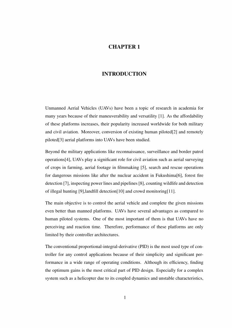
Unmanned Aerial Vehicles (UAVs) have been a topic of research in academia for

many years because of their maneuverability and versatility [1]. As the affordability

of these platforms increases, their popularity increased worldwide for both military

and civil aviation. Moreover, conversion of existing human piloted[2] and remotely

piloted[3] aerial platforms into UAVs have been studied.

Beyond the military applications like reconnaissance, surveillance and border patrol

operations[4], UAVs play a significant role for civil aviation such as aerial surveying

of crops in farming, aerial footage in filmmaking [5], search and rescue operations

for dangerous missions like after the nuclear accident in Fukushima[6], forest fire

detection [7], inspecting power lines and pipelines [8], counting wildlife and detection

of illegal hunting [9],landfill detection[10] and crowd monitoring[11].

The main objective is to control the aerial vehicle and complete the given missions

even better than manned platforms. UAVs have several advantages as compared to

human piloted systems. One of the most important of them is that UAVs have no

perceiving and reaction time. Therefore, performance of these platforms are only

limited by their controller architectures.

The conventional proportional-integral-derivative (PID) is the most used type of con-

troller for any control applications because of their simplicity and significant per-

formance in a wide range of operating conditions. Although its efficiency, finding

the optimum gains is the most critical part of PID design. Especially for a complex

system such as a helicopter due to its coupled dynamics and unstable characteristics,

1

designing and tuning of PID controllers are very hard in practice. Besides, even a well

designed PID controller with fixed parameters can hardly adapt to uncertainties and

changing flight conditions[12]. Therefore, operation range of PID controllers are re-

stricted with the initial gain settings. For these reasons, self-tuning and adaptive PID

controllers are used in literature to design, tune and improve the control performance

of PID controllers[13].

In this study, the Bell UH-1 Huey (UH-1H) helicopter which is a two-bladed military

helicopter powered by a single turboshaft engine and also commonly used by Turkish

Land Forces Aviation is converted to an unmanned platform in virtual environment by

developing a full flight controller for hover and forward flight conditions. Then, a PID

gain update law using linear least squares regression is presented as a new adaptive

control method for autonomous helicopters. In addition, future prediction analysis

are conducted for error dynamics of the closed loop system using recursive linear

least squares regression. Combining these two concepts with classical PID controller,

an intelligent PID controller is acquired. Excluding the velocity controllers, PID

controllers of the flight controller are replaced by the newly developed intelligent

controller. Thus, a new intelligent flight controller is obtained with model prediction

and adaptation abilities.

After completing the design of the intelligent flight controller, the first flight con-

troller that has no adaptation ability and the new intelligent flight controller are tested

with same PID gains by conducting several challenging maneuvers to demonstrate

the effectiveness of the new intelligent flight controller.

1.1 Literature Survey

Self tuning, adaptive and intelligent controller concepts are well known and widely

used in literature. In 1997, an intelligent helicopter controller using artificial neural

network, genetic algorithm and fuzzy logic was developed by S. Zein-Sabatto and Y.

Zheng[14]. Lee et al. implemented fuzzy neural network as an adaptation method

for PID controllers in 2002 [12]. In 2005, Zhang et al. used radial basis function

(RBF) neural networks for PID gain adaptation [13]. Sanchez et al. used fuzzy logic

2

to adjust the PID controller gains for an autonomous mini-helicopter in 2007 [15].

O. Tarimci developed a neural network based adaptive flight controller for AH-1S

helicopter using model inversion technique in 2009 [16]. This study is the starting

point of this thesis. In 2011, Sadeghzadeh et al. developed a trajectory tracking

controller for a quadrotor helicopter using gain-scheduled PID and model reference

adaptive control (MRAC)[17]. A self tuning PID controller for a twin rotor system

was developed by P. Sahu and S. K. Pradhan in 2014. [18]. In 2015, H. Gao et al.

developed a fuzzy adaptive PD controller for a quadrotor UAV[19].

Least squares regression is also popular in literature for adaptation and optimization

of PID gains. In 1985, A. Brickwedde used RLS for PID pole assignment to control

the speed and postion of an electrical drive with a microprocessor[20]. E. Poulin et al.

used damped version of recursive linear least square regression (DLS) to find the op-

timum gains of the PID controller for a given transfer function in 1996 . In this study,

gains of PID were calculated directly from the least squares optimization using the

process gain, time constant and time delay in the coefficient matrix of DLS[21]. In

1997, a combined method of least-squares estimation, Newton–Raphson search tech-

nique and Ziegler-Nichols formulas for self tuning of PID controllers was proposed

by Rad et al. [22]. In 1999, Mitsukura et al. also used Recursive Least Squares (RLS)

algorithm to find the process gain, time constant and time delay of a PID controller

from the deviation of RLS coefficient matrix[23]. In 2000, Grassi et al. used Least

Squares Regression for loop shaping of PID controller[24]. In 2004, J. Chen and Y.

Cheng used Partial Least Squares algorithm to find the process gain, time constant

and time delay of a PID controller from the deviation of RLS coefficient. Differ-

ently, they used error as a state instead of using state of the system in least square

regression[25]. Again Recursive Least Squares (RLS) algorithm was used to find the

process gain, time constant and time delay of a PID controller from the deviation

of RLS coefficient matrix with a different gain update formula by T. Yamamoto and

S. L. Shah in 2007 [26]. In 2008, Wanfeng et al. used least squares support vector

machines with RBF kernel to model the gradient of the system error with respect to

control input and update the PID gains using this gradient[27]. Similarly, Zhao et al.

used least squares support vector machines with RBF kernel to design an intelligent

PID controller in 2009[28]. Recent research have focused on non-linear least squares

3

regression for adaptive control. In 2014, Wilson et al. applied non-linear least squares

regression for trajectory optimization[29].

1.2 Contribution of this Thesis

In this thesis, an intelligent flight controller is developed for a full size helicopter that

has the ability to perform challenging maneuvers better than a human pilot. As an

original contribution to the literature, a new PID gain update law using Linear Least

Squares Regression is proposed. In addition, prediction of future values of the closed

loop error is achieved by using Recursive Linear Least Squares Regression. Com-

bining these two concepts, a new intelligent controller for autonomous helicopters is

obtained that has an effective PID gain scheduling capability.

1.3 Thesis Structure

The structure of this thesis is as follows, Adaptation and model prediction concepts

are given in Chapter 1 as an introduction. In addition, results of literature survey about

adaptive PID control methods and least squares regression applications for adaptive

control are mentioned in Chapter 1.

In Chapter 2, Least Squares Regression and Recursive Least Squares Regression

methods are explained in detail. The limitations of Least Squares Regression are also

described in this chapter. In addition, implementation of Recursive Least Squares

Regression for prediction is mentioned in this chapter.

The main contribution of this thesis which is a least squares based adaptive controller

with a new PID gain update law is presented in Chapter 3. Besides, an intelligent

controller design that is the second contribution of this thesis is expressed in this

chapter.

Architecture of the Intelligent Flight Controller is described in Chapter 4. Implemen-

tation of the intelligent controller is also explained in this chapter.

Modeling the UH-1H is described in Chapter 5. Mass, inertia and geometric data of

4

UH-1H are given in this chapter.

Chapter 6 includes the simulation results of six challenging maneuvers for both a

flight controller with classical PID controllers and the Intelligent Flight Controller.

Finally, a brief summary of the thesis is given in Chapter 7. Conclusions and future

work are also discussed in this chapter.

5

CHAPTER 2

METHODOLOGY

In this study, an adaptive and model predictive PID controller is developed by using

Least Squares Regression which is widely used for online adaptive control and real

time parameter estimation [30]. Least Squares Regression finds an optimum solution

by minimizing the sum of the squares of the errors for overdetermined systems [31].

This method is used to derive a new PID gain update law that is detailed in Chapter

3 and also an optimum statistical model to predict the future value of a state from

its previous values for an asymptotically stable closed loop system. For a given time

frame, Least Squares Regression is used recursively to predict the next future values.

This recursive usage is called as Recursive Least Squares Regression in literature

[32].

2.1 Linear Least Squares Regression

A state can be modeled using the past values of itself within a given time frame P[33].

xk = a0 + a1 · xk−1 + a2 · xk−2 + · · ·+ an · xk−n + ∆k (2.1)

αT =[a0 a1 a2 · · · an

](2.2)

ΦTk =

[1 xk−1 xk−2 · · · xk−n

](2.3)

7

xk = ΦTkα + ∆k (2.4)

where ∆k is the modeling error,

∆k = xk − ΦTkα (2.5)

Sum of the least squares of the modeling errors for N data points can be expressed as

follows,

E(α,N) =N∑k=1

(xk − ΦTkα)2 (2.6)

E(α,N) =N∑k=1

[(xk − ΦT

kα)T (xk − ΦTkα)]

E(α,N) =N∑k=1

(xTk xk − xTkΦTkα− αTΦkxk + αTΦkΦ

Tkα) (2.7)

Note that xk = ΦTkα + ∆k and (αTΦkxk)

T = xTkΦTkα,

(αTΦkxk)T = xTk (xk −∆k) (2.8)

Since xk is a (1× 1) vector, αTΦkxk is a scalar value and equal to its own transpose.

αTΦkxk = xTkΦTkα (2.9)

Then equation (2.7) can be simplified as,

E(α,N) =N∑k=1

(xTk xk − 2αTΦkxk + αTΦkΦTkα) (2.10)

Differentiating both sides with respect to α,

∂E

∂α=

N∑k=1

(−2Φkxk + 2ΦkΦTkα)

∂E

∂α= 2

N∑k=1

(−Φkxk + ΦkΦTkα) (2.11)

8

Second derivative of E(α,N) with respect to α,

∂2E

∂α2= 2

N∑k=1

(ΦTkΦk) (2.12)

Due to the definition of Φk, Φk cannot be a zero vector and the multiplication of a

non-zero vector Φk by its transpose always gives a positive value.

∀ Φk, (ΦTkΦk) > 0 =⇒ ∂2E

∂α2> 0 (2.13)

Therefore, E(α,N) always decreases as k → N and has a global minimum at k = N

for N data points.

To satisfy the necessary condition for a relative extremum, equating the first derivative

of E(α,N) to zero is enough to find the best modeling parameter αk that minimizes

E(α,N) according to the second derivative test of E(α,N).

Then the equation (2.11) becomes,

0 =N∑k=1

(−Φkxk + ΦkΦTk αk) (2.14)

Rearranging for the modeling paramater αk,

N∑k=1

(Φkxk) =N∑k=1

(ΦkΦTk αk)

αk =

(N∑k=1

ΦkΦTk

)−1( N∑k=1

Φkxk

)(2.15)

2.2 Recursive Linear Least Squares Regression

Assume αT =[a0 a1 a2 · · · an

]is constant for a limited time frame R, then xk

can be used to calculate the next R states.

xk = a0 + a1 · xk−1 + a2 · xk−2 + · · ·+ an · xk−n

xk+1 = a0 + a1 · xk + a2 · xk−1 + · · ·+ an · xk−n+1

9

xk+2 = a0 + a1 · xk+1 + a2 · xk + · · ·+ an · xk−n+2

...

xk+R = a0 + a1 · xk+R−1 + a2 · xk+R−2 + · · ·+ an · xk−n+R

The recursive least squares algorithm allows the prediction of the next R future states

assuming a constant modeling parameter α which is calculated from equation (2.15)

using xk and the P past values of x.

0

0.2

0.4

0.6

0.8

1

0 0.5 1 1.5 2 2.5 3

y(t

)

time (s)

Predicted ResponseActual Response

Figure 2.1: Prediction of Unit Step Input

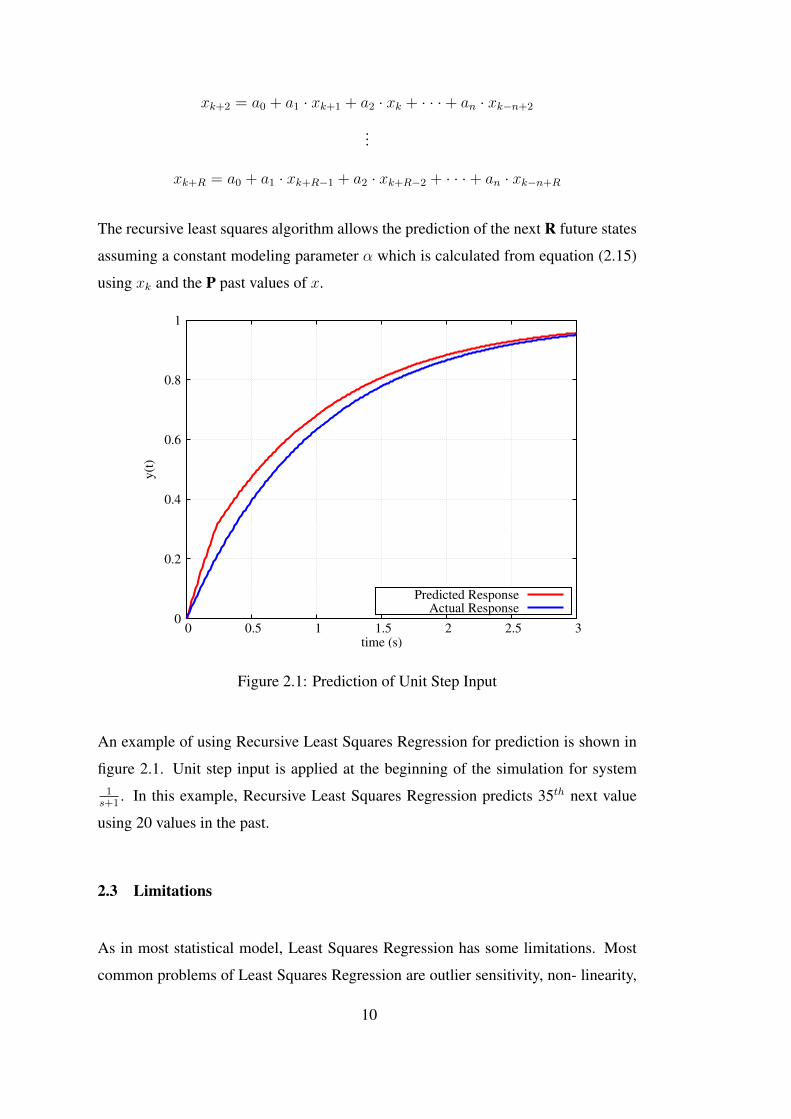
An example of using Recursive Least Squares Regression for prediction is shown in

figure 2.1. Unit step input is applied at the beginning of the simulation for system1s+1

. In this example, Recursive Least Squares Regression predicts 35th next value

using 20 values in the past.

2.3 Limitations

As in most statistical model, Least Squares Regression has some limitations. Most

common problems of Least Squares Regression are outlier sensitivity, non- linearity,

10

dealing with high numbers of variables, dependencies between independent variables,

heteroskedasticity and variances in independent variables.[34].

Figure 2.2: Outliers in a Data Set

Outlier is a distinct point in a data set which lies outside of the overall pattern[35] as

shown in figure 2.2. For a continuous system with a very tiny step size, outliers are

not expected and hence outliers does not create a problem for the least square regres-

sion. Hence, choosing a step size of 0.01 seconds and using a continuous integration

method like Euler on MATLAB Simulink is enough to minimize outliers. Effect of

non-linearity of the system is eliminated by choosing a tiny step size and decreasing

the number of independent variables of regression. Modeling errors due to high num-

bers of variables is avoided by choosing the number of independent variables much

smaller than the number of available data points[34].

11

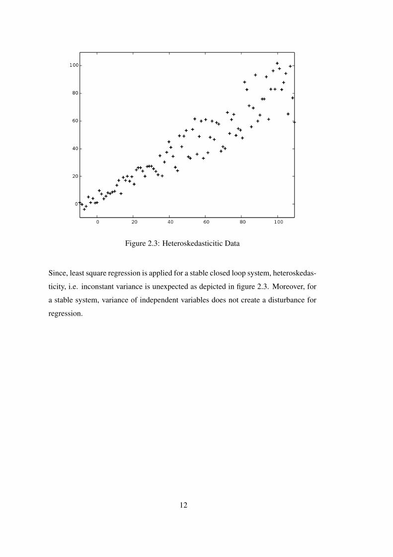
Figure 2.3: Heteroskedasticitic Data

Since, least square regression is applied for a stable closed loop system, heteroskedas-

ticity, i.e. inconstant variance is unexpected as depicted in figure 2.3. Moreover, for

a stable system, variance of independent variables does not create a disturbance for

regression.

12

CHAPTER 3

LEAST SQUARES BASED ADAPTIVE CONTROL

Adaptive control is achieved by modeling the error dynamics and finding the optimum

PID gains using Least Squares Regression. For a quick gain optimization, proper

initial PID gains should be used. It is also possible to start from any initial guess like

a system identification process. In this thesis, an asymptotically stable closed loop

system is selected as a starting point to increase the success of the optimization. In

addition, the limitations of Least Squares Regression which are mentioned in Chapter

2 restrict the usage of this method for mostly stable systems.

3.1 Modeling Error Dynamics

The output of conventional PID controller is the weighted sum of proportional, inte-

gral and derivative channels.

uk = KP ek +KI

∫ek dt+KD ek (3.1)

whereKP ,KI andKD are the proportional, integral and derivative gains respectively.

Error that is minimized by PID controller is the difference between the desired and

the current values of a state.

ek = xdk − xk (3.2)

Each channel of a PID controller is modeled using Least Square Regression as shown

below,

Proportional Channel:

ek = P0 + P1xk−1 + P2xk−2 + . . .+ Pnxk−n + ∆P k (3.3)

13

Integral Channel:∫ek dt = I0 + I1xk−1 + I2xk−2 + . . .+ Inxk−n + ∆Ik (3.4)

Derivative Channel:d ekdt

= D0 +D1xk−1 +D2xk−2 + . . .+Dnxk−n + ∆Dk (3.5)

The modeling errors of the each channel are ∆P k, ∆Ik and ∆Dk respectively.

Error dynamics is in matrix form,

ek∫ek dt

ek

=

P0 P1 P2 · · · Pn

I0 I1 I2 · · · In

D0 D1 D2 · · · Dn

1

xk−1

xk−2

...

xk−n

+

∆P k

∆Ik

∆Dk

(3.6)

3.2 PID Gain Update Law

Modeling errors are used for updating the PID gains using a learning rate η for each

channel as follows,

∆KP k = ηP ∆P k (3.7)

∆KIk = ηI ∆Ik (3.8)

∆KDk = ηD ∆Dk (3.9)

PID gain update law in matrix form,

∆KP k

∆KDk

∆KIk

=

ηP 0 0

0 ηI 0

0 0 ηD

ek∫ek dt

ek

−P0 P1 P2 · · · Pn

I0 I1 I2 · · · In

D0 D1 D2 · · · Dn

1

xk−1

xk−2

...

xk−n

(3.10)

14

An adaptive controller is obtained from the modeling errors of the Linear Least

Squares Regression of the error dynamics. These modeling errors are multiplied by a

learning rate for each channel and added to the gains of the PID controller to calculate

the new PID gains for the next time step as shown below,

KP k+1 = KP k + ∆KP k (3.11)

KIk+1 = KIk + ∆KIk (3.12)

KDk+1 = KDk + ∆KDk (3.13)

According to the proof in section 2.1, as the number of data points for least squares re-

gression increases, the modeling error of the least square regression decreases. Thus,

increasing the number of data points that have similar variance in a closed domain

of the target state minimizes the regression error. An asymptotically stable system

satisfies this condition. As stated in Chapter 2, Least Square Regression is applied

for an asymptotically stable closed loop system. Therefore, the least squares based

adaptive controller is also asymptotically stable and PID gain updates go to zero for

sufficiently small learning rates.

The limitations of this new PID gain update law depend on the limitations of the

Linear Least Squares Regression that is mentioned in Chapter 2.

15

Figure 3.1: Block Diagram of the Intelligent Controller

3.3 Intelligent Controller Design

Classical PID controller design is improved by adding prediction and adaptation ca-

pabilities that convert the PID to an intelligent controller as depicted in figure 3.1.

In order to achieve this, an error predictor is developed using Recursive Linear Least

Squares Regression which predicts the 35th future value of the error from 20 past

values of the error. Instead of feeding the instantaneous error, this predicted error is

used as an input to the controller. In addition to the predictor, a state history block

is implemented to log the 20 past values of the state. Error dynamics of the system

is modeled using these past values with Least Squares Regression. After adaptation

is completed in Least Squares based Adaptive Controller by updating PID gains with

the errors of the error dynamics as explained in equation 3.10, the optimum PID gains

are obtained.

16

CHAPTER 4

INTELLIGENT FLIGHT CONTROLLER ARCHITECTURE

The main objective of this thesis is to design an intelligent model prediction controller

for an autonomous helicopter. For this purpose, adaptive controller architectures [16]

and [36] are analysed and improved without using a neural network for adaptation.

In addition, the controller is optimized for both hover and forward flight conditions.

Finally, an intelligent model prediction controller is implemented and an Intelligent

Flight Controller (IFC) is obtained.

4.1 Flight Controller Design

As in the previous controller design[16], flight controller consist of a trajectory gen-

erator, outer loop for position control and inner loop for attitude control. In addition,

body angular velocity controller is added as a third loop. Decoupling the position and

attitude control, improves the controller efficiency for faster rotational dynamics. In

addition to decoupling, the controller has two command filters for both inner loop and

outer loop to eliminate oscillations. Also, an actuator model is included in the inner

loop for swashplate dynamics.

The previous design[16] has an effective feed forward mechanism for PID controller

that increases the performance of the controller significantly. This feed forward mech-

anism is arisen by the summation of the second derivative of the command with the

control output of PID and thus an improved PID controller (I-PID) is obtained as

illustrated in figure 4.1.

17

Figure 4.1: Block Diagram of the I-PID Controller

In the previous design[16], model inversion technique is used to generate control in-

puts. An error always occurs due to the approximations for inversion. Moreover, as

the complexity and fidelity of the model increases, it gets harder to invert the model

and model inversion error increases. An online learning capable neural network based

adaptive controller is used to overcome this modeling error in the previous study[16].

In spite of using an adaptive controller, the model inversion has still a disadvantage

that the stability and control matrices are assumed to be time invariant and linearized

for only one flight condition. Because of this assumption, as flight condition changes

from the initial trim point where the linearization is done, model inversion error in-

creases. Therefore, since the model inversion method has a restricted usage due to the

assumption of the constant stability and the control matrices of the system, instead of

using the model inversion method in the inner loop, a Body Angular Velocity Con-

troller (BAVC) is implemented as a third loop (most-inner loop) for the new flight

controller.

18

4.1.1 Actuator Model

A second order filter is used as an actuator model. The natural frequency of the actu-

ator model is chosen as 70 rad/s to be faster than helicopter dynamics. The damping

ratio is selected as 0.6 to prevent the flattening out the dynamics. In addition, the ac-

tuator model has angle and rate saturations to model the actual swashplate dynamics.

The transfer function of the actuator model is as shown below,

4900

s2 + 84 s+ 4900(4.1)

4.1.2 Command Filter

A second order command filter is also used for both outer and inner loops to eliminate

the control oscillations. The natural frequency of the command filter is chosen as

1 rad/s to have a slower dynamics than the controllers of the position and attitude

channels. The damping ratio of the command filter is chosen as 0.8 to have an extra

feed forward effect for controllers.The transfer function of the command filter is as

follows,

1

s2 + 1.6 s+ 1(4.2)

Actuator model and command filter settings are taken from the previous study. But,

there is an obligatory change for the Acutator Model, since the helicopter is AH-1S

in the previous thesis[16] and has different control margins from UH-1H. Actuator

limits of UH-1H are shown in the table 4.1. These limits are obtained during the

development of Heli-Dyn[37].

Table 4.1: Actuator Limits

Longitudinal LateralSwashplate Collective Swashplate Pedal

Angle Limit (deg) ± 8 0 - 20 ± 8 -5 - 20Rate Limit (deg/s) ± 10 ± 10 ± 10 ± 10

19

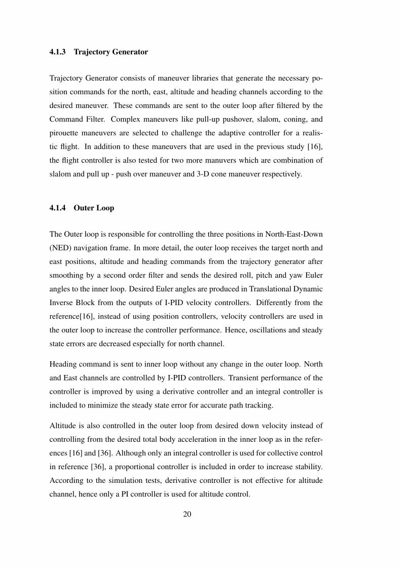
4.1.3 Trajectory Generator

Trajectory Generator consists of maneuver libraries that generate the necessary po-

sition commands for the north, east, altitude and heading channels according to the

desired maneuver. These commands are sent to the outer loop after filtered by the

Command Filter. Complex maneuvers like pull-up pushover, slalom, coning, and

pirouette maneuvers are selected to challenge the adaptive controller for a realis-

tic flight. In addition to these maneuvers that are used in the previous study [16],

the flight controller is also tested for two more manuvers which are combination of

slalom and pull up - push over maneuver and 3-D cone maneuver respectively.

4.1.4 Outer Loop

The Outer loop is responsible for controlling the three positions in North-East-Down

(NED) navigation frame. In more detail, the outer loop receives the target north and

east positions, altitude and heading commands from the trajectory generator after

smoothing by a second order filter and sends the desired roll, pitch and yaw Euler

angles to the inner loop. Desired Euler angles are produced in Translational Dynamic

Inverse Block from the outputs of I-PID velocity controllers. Differently from the

reference[16], instead of using position controllers, velocity controllers are used in

the outer loop to increase the controller performance. Hence, oscillations and steady

state errors are decreased especially for north channel.

Heading command is sent to inner loop without any change in the outer loop. North

and East channels are controlled by I-PID controllers. Transient performance of the

controller is improved by using a derivative controller and an integral controller is

included to minimize the steady state error for accurate path tracking.

Altitude is also controlled in the outer loop from desired down velocity instead of

controlling from the desired total body acceleration in the inner loop as in the refer-

ences [16] and [36]. Although only an integral controller is used for collective control

in reference [36], a proportional controller is included in order to increase stability.

According to the simulation tests, derivative controller is not effective for altitude

channel, hence only a PI controller is used for altitude control.

20

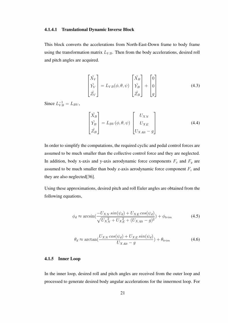
4.1.4.1 Translational Dynamic Inverse Block

This block converts the accelerations from North-East-Down frame to body frame

using the transformation matrix LV B. Then from the body accelerations, desired roll

and pitch angles are acquired.

XV

YV

ZV

= LV B(φ, θ, ψ)

XB

YB

ZB

+

0

0

g

(4.3)

Since L−1V B = LBV ,

XB

YB

ZB

= LBV (φ, θ, ψ)

UXN

UXE

UXAlt − g

(4.4)

In order to simplify the computations, the required cyclic and pedal control forces are

assumed to be much smaller than the collective control force and they are neglected.

In addition, body x-axis and y-axis aerodynamic force components Fx and Fy are

assumed to be much smaller than body z-axis aerodynamic force component Fz and

they are also neglected[36].

Using these approximations, desired pitch and roll Euler angles are obtained from the

following equations,

φd ≈ arcsin(−UXN sin(ψd) + UXE cos(ψd)√UX

2N + UX

2E + (UXAlt − g)2

) + φtrim (4.5)

θd ≈ arctan(UXN cos(ψd) + UXE sin(ψd)

UXAlt − g) + θtrim (4.6)

4.1.5 Inner Loop

In the inner loop, desired roll and pitch angles are received from the outer loop and

processed to generate desired body angular accelerations for the innermost loop. For

21

this process, the relation matrix between Euler angle rates and body angular velocities

is used as shown in equation 4.7.

p

q

r

=

1 0 −sin(θ)

0 cos(φ) sin(φ) cos(θ)

0 −sin(φ) cos(φ) cos(θ)

φ

θ

ψ

(4.7)

Since the integral controller has adverse effects for attitude control, for each attitude

channel an I-PD controller is used. Transient performance of the attitude channels are

improved by implementing a derivative controller for each channel. The commands

for attitude controllers are passed through the command filter and taken by Euler

Angle Controller (EAC) which consists of three I-PD attitude controllers. The outputs

of EAC are sent to the innermost loop to generate longitudinal cyclic, lateral cyclic

and pedal controls from desired body angular velocities.

Inner loop also includes the innermost loop that is responsible from controlling the

body angular velocities.

4.1.5.1 Innermost Loop

As mentioned before, necessary control inputs are generated according to the desired

body angular velocities which are received from the inner loop. Th innermost loop

or in other words Body Angular Velocity Controller (BAVC) generates longitudinal

cyclic, lateral cyclic and pedal controls from desired body angular velocities using

I-PID controllers for each channel.

4.2 Controller Optimization for Hover and Forward Flight

The new flight controller is capable of both flying at hover and forward flight condi-

tions. Therefore, gain scheduling is used for the velocity controller and the command

filter to optimize the transition between hover and forward flight. The gain scheduling

is achieved by setting nonlinear gain equations. First, variable derivative and integral

gains are used for east velocity controller rather than constant ones. The following

22

equations are used for the gain scheduling,

I = min

(VTotal250

, 1

)+ 0.02 ·

(VTotal

10

)2

(4.8)

D =0.7 · VTotal + 13

8+ 0.1 ·min

(VTotal

50, 1

)(4.9)

where velocities are in knots and VTotal is obtained from,

VTotal = min(√

V 2N + V 2

E , 50√

2)

(4.10)

Second, damping ratios for north and east channels of the command filter in the outer

loop are changed according to the 4.11 and 4.12 instead of using constant values. The

damping ratios are increased with respect to forward flight speed as shown in figure

4.2 to increase the stability of the transition from hover to forward flight.

ξNorth = 0.8 + min(0.001 · |∆VNorth|2.1, 30) (4.11)

ξEast = 0.8 + min(0.001 · |∆VEast|2.5, 30) (4.12)

0

5

10

15

20

25

30

35

0 10 20 30 40 50 60 70 80 90

Dam

ping

Rat

io

Commanded Absolute Change in North Velocity (knots)

0

5

10

15

20

25

30

35

0 10 20 30 40 50 60 70 80 90

Dam

ping

Rat

io

Commanded Absolute Change in East Velocity (knots)

Figure 4.2: Command Filter Damping Changes for North and East Veloctiy Com-

mands

23

Figure 4.3: Intelligent Flight Controller Design

24

4.3 Intelligent Controller Implementation

In this study, capabilities of I-PID controller are extended by adding model prediction

and adaptation abilities which leads to an intelligent controller as described in Chapter

3. Each of the I-PID controllers in the inner loop (EAC and BAVC) is replaced with

this intelligent I-PID controller. Thus, a new adaptive and model predictive Intelligent

Flight Controller (IFC) is acquired. As mentioned before, IFC has three control loops

as shown in figure 4.3. The outer loop of IFC has only I-PID controllers. But, the

inner and the innermost loop contains Intelligent I-PID Controllers.

25

CHAPTER 5

MODELING HELICOPTER

For the simulation tests, the UH-1H helicopter is chosen since it is a known heli-

copter in literature[38]. A software for rotorcraft modeling and simulation called

Heli-Dyn[37] is used for modeling the helicopter.

Heli-Dyn was firstly developed by AeroTIM with the support of TUBITAK and KOS-

GEB. The author of this thesis is also a member of the core development team of

the first several versions of Heli-Dyn. It is a dynamic modeling tool which is capa-

ble of modeling a helicopter, trimming, linearizing around any trim points and also

conducting basic performance analysis that supports for different ISA temperature

conditions as shown in figure 5.1. In addition, any external simulation and software

environments can be integrated with Heli-Dyn. Providing geometric, inertial and

aerodynamic data any helicopter can be modeled using this software.

Heli-Dyn uses a component build-up technique for generating the whole helicopter

model. In component built-up method, the forces and moments generated by each

component of the helicopter are integrated at the center of gravity of the helicopter

leading the usage of 6-DOF (Degree of Freedom) rigid body dynamics. This method

allows an interchangeability for the users and developers. Any component can be

replaced with a more sophisticated high fidelity model or there may be lots of versions

for a specific component with different fidelities as shown in figure 5.2.

27

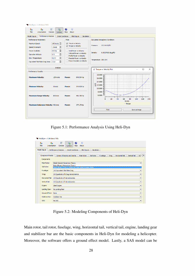
Figure 5.1: Performance Analysis Using Heli-Dyn

Figure 5.2: Modeling Components of Heli-Dyn

Main rotor, tail rotor, fuselage, wing, horizontal tail, vertical tail, engine, landing gear

and stabilizer bar are the basic components in Heli-Dyn for modeling a helicopter.

Moreover, the software offers a ground effect model. Lastly, a SAS model can be

28

added to ease the usage of the helicopter or for testing purposes.

Each model component includes different models with various fidelities. For the

main rotor component, there are two versions; the well known "Minimum Complex-

ity" model[39] which uses Blade Element Momentum Theory and Blade Element

Moementum with Peters-He Inflow model[40]. These models were validated by the

development team in 2008[41]. The minimum complexity model uses first order flap-

ping, uniform inflow and an iterative approach to the classic momentum and Glauert

Theories for force and moment calculations. Peters-He Inflow model of Heli-Dyn

uses 3-state Peters-He inflow models for main rotor blade element solutions.

The main difference between these two main rotor models is the main rotor thrust

and inflow calculations. While, minimum complexity accepts flow distribution as

uniform and calculates thrust from momentum theory, Peters-He inflow distribution

model computes thrust by sectioning the main rotor blades. For real time performance

considerations, section number is limited to three for the inflow model in Heli-Dyn.

The Peters-He inflow model has some advantages on blade element momentum mod-

els like minimum complexity such that it generates an improved pressure distribution

across a rotor plane including tip loss[41]. In this thesis, the minimum complexity

model is used for the main rotor and tail rotor components. Geometric inputs for

the main rotor component and stabilizer bar are given in figure 5.3 and the tail rotor

geometry inputs are specified as shown in figure 5.4

29

Figure 5.3: Geometric Inputs for Main Rotor Component

The data of geometric inputs of main rotor and tail rotor are the default values in the

HeliDyn software for UH-1H and are validated in the study[41].

Figure 5.4: Geometric Inputs for Tail Rotor Component

Other basic components such as wings, horizontal stabilizer, vertical tail, etc. are

modeled by simple aerodynamic equations with constant coefficients[42].

Mass and inertia data are taken from the reference[38] as stated in figure 5.5.

30

Figure 5.5: Mass and Inertia Data of UH-1H

In this study, Heli-Dyn v1.04 is used to model the UH-1H with the default geometry

and components settings as shown below,

• Main Rotor: Blade Element Momentum Theory

• Tail Rotor: Blade Element Momentum Theory

• Fuselage: 3-D Equivalent Flat Plate Drag

• Wing: 2-D Quadratic Lift Aerodynamics

• Horizontal Tail: 1-D Quadratic Lift Aerodynamics

• Vertical Tail: 1-D Quadratic Lift Aerodynamics

• Engine: Ideal Engine

• Landing Gear: None

• Ground Effect: None

• Stabilizer Bar: Default

• SAS: None

Since all simulations start from 1000 ft hover and the minimum altitude for each

maneuver is higher than 750 ft during flight, ground effect and landing gear models

are not used. Using these settings, UH-1H model is trimmed at 1000 ft for hover as

31

depicted in figure 5.6. The simulation tests are started from this trim point with the

initial conditions and corresponding trim controls.

Figure 5.6: Hover Trim Results of UH-1H at 1000 ft

32

CHAPTER 6

SIMULATION RESULTS

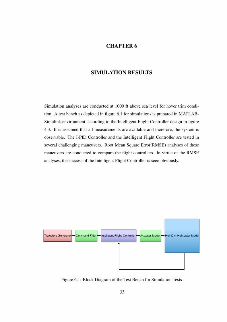
Simulation analyses are conducted at 1000 ft above sea level for hover trim condi-

tion. A test bench as depicted in figure 6.1 for simulations is prepared in MATLAB-

Simulink environment according to the Intelligent Flight Controller design in figure

4.3. It is assumed that all measurements are available and therefore, the system is

observable. The I-PID Controller and the Intelligent Flight Controller are tested in

several challenging maneuvers. Root Mean Square Error(RMSE) analyses of these

maneuvers are conducted to compare the flight controllers. In virtue of the RMSE

analyses, the success of the Intelligent Flight Controller is seen obviously.

Figure 6.1: Block Diagram of the Test Bench for Simulation Tests

33

6.1 Root Mean Square Analysis

The root mean square is a special case of power mean. The power mean is a general-

ized mean which is in the form,

Mp(a1, a2, . . . , an) =

(1n

n∑k=1

apk

)1/p

(6.1)

where ak ≥ 0 and p is a real number in the domain [−∞,+∞].

And for p = 2 which is the M2 power mean is the root mean square (RMS),

M2(a1, a2, . . . , an) =

√√√√ 1

n

n∑k=1

a2k (6.2)

The RMS can be extended to RMSE for error analysis using the equation 3.2.

RMSE =

√√√√ 1

n

n∑k=1

(xd − x)2 (6.3)

The RMSE analysis is used for comparing difference between the desired and actual

values of the position and attitude channels to find the best flight controller for each

maneuver. The results of the RMSE analysis for each maneuver are illustrated in

figure A.1.

6.1.1 RMSE Analysis for a Single State

For comparing two tests for a single state like roll angle, quotient of the RMSE values

of the state is used as shown below,

S = 100×(

1− RMSEnewRMSEref

)(6.4)

where S is the success ratio, RMSEref is the RMSE value of the reference test and

RMSEnew is the RMSE value of the new test.

6.1.2 RMSE Analysis for Multiple States

For comparing two tests for multiple states like the combination of roll, pitch and yaw

angles as attitude, ratio of Euclidean Norms of the RMSE values of these states are

34

used as shown below,

S = 100×

(1−

√RMSE2

1new+RMSE2

2new+ · · ·+RMSE2

nnew

RMSE21ref

+RMSE22ref

+ · · ·+RMSE2nref

)(6.5)

where S is the success ratio, RMSEnrefis the RMSE value of the reference test for

nth state in the comparison list and RMSEnrefis the RMSE value of the new test for

nth state in the comparison list.

6.2 Maneuvers

As mentioned before, six challenging maneuvers are selected to demonstrate the

adaptation abilities of the Intelligent Flight Controller with respect to the I-PID con-

troller with constant gains. These maneuvers are pull up - push over, slalom, pull-up -

push over - slalom, coning, pirouette and 3-D cone respectively. All these maneuvers

are started from hover trim point at 1000 ft above sea level with the initial trim con-

trols and simulated at 100 Hz using Euler integration method in MATLAB Simulink.

As described in Chapter 4, the Intelligent Flight Controller has ability to change the

Inner Loop controller gains during flight. Both I-PID and the Intelligent Flight Con-

troller are started from the same gains and performance of the controllers are ana-

lyzed.

Initial controller gains for the inner loop are selected as,

• Euler Angle Controller

– φ Channel: KP=10,KI=0,KD=5

– θ Channel: KP=10,KI=0,KD=5

– ψ Channel: KP=10,KI=0,KD=5

• Body Angular Velocity Controller

– p Channel: KP=20,KI=1,KD=10

– q Channel: KP=30,KI=1,KD=15

– r Channel: KP=20,KI=1,KD=10

35

The intelligent controller needs a closed loop stable system due to the limitations of

Least Squares Regression as stated in Chapter 2 and 3. Otherwise, intelligent con-

troller may still adapt and control the helicopter if Least Squares Regression succeeds

to model the error dynamics of the unstable system. Therefore, these initial PID

gains are chosen after testing them to have a stable system at least 30 seconds for

each maneuver with I-PID controller. After determination of the initial PID gains,

six complex maneuvers are tested for both controllers. The first three maneuvers and

the last one are conducted for 300 seconds. However, simulations for coning and

pirouette maneuvers are limited to 120 seconds for both controllers because of the

difficulty of these maneuvers.

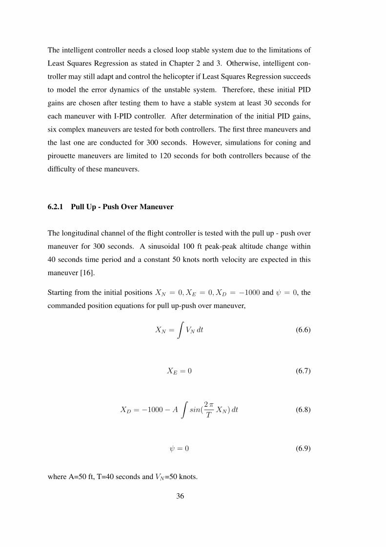
6.2.1 Pull Up - Push Over Maneuver

The longitudinal channel of the flight controller is tested with the pull up - push over

maneuver for 300 seconds. A sinusoidal 100 ft peak-peak altitude change within

40 seconds time period and a constant 50 knots north velocity are expected in this

maneuver [16].

Starting from the initial positions XN = 0, XE = 0, XD = −1000 and ψ = 0, the

commanded position equations for pull up-push over maneuver,

XN =

∫VN dt (6.6)

XE = 0 (6.7)

XD = −1000− A∫sin(

2π

TXN) dt (6.8)

ψ = 0 (6.9)

where A=50 ft, T=40 seconds and VN=50 knots.

36

960

980

1000

1020

1040

0 5000 10000 15000 20000

Alt

itude

Posi

tion (

ft)

North Position (ft)

Commanded TrajectoryI-PID Controller

Intelligent Controller

Figure 6.2: Trajectory of the Helicopter on X-Z Plane

The I-PID controller can stand for about 100 seconds without any adaptation, but

the chosen initial gains are not suitable for this maneuver and the helicopter crashes

before the simulation ends. However, the Intelligent Flight Controller is adapted itself

quickly and controls the helicopter until the end of the simulation. Divergent path

followed by I-PID controller and also the trajectory followed by the Intelligent Flight

Controller are shown in in figure 6.2.

Adaptation of PID gains of the Euler Angle Controller of the Intelligent Flight Con-

troller is shown in figure 6.3. Derivative gains are nearly constant and integral gains

are applied periodically after learning is completed. Differently, there are oscillations

in proportional gains, but the amplitude of the oscillations are insignificant.

37

9.75 9.8

9.85 9.9

9.95 10

10.05 10.1

10.15

0 50 100 150 200 250 300

P G

ain

time (s)

PhiTheta

Psi

0

0.1

0.2

0.3

0.4

0.5

0.6

0.7

0 50 100 150 200 250 300

I G

ain

time (s)

PhiTheta

Psi

4.5 4.6 4.7 4.8 4.9

5 5.1 5.2 5.3

0 50 100 150 200 250 300

D G

ain

time (s)

PhiTheta

Psi

Figure 6.3: Adaptation History of the Euler Angle Controller Gains

The amplitude of oscillations in proportional channel for theta control is larger than

other channels. This difference is expected since the maneuver challenges the longi-

tudinal stability of the controller directly by periodic climbs and dives.

Initial short-time peaks for integral and derivative gains of theta and psi channels are

related with the adaptation process and transition from hover to forward flight. As

helicopter reaches to 50 knots forward speed, adaptation gets easier and these peaks

fade out.

The stability of the PID gains of the Euler Angle Controller of the Intelligent Flight

Controller provides a correct trajectory tracking as seen in figure 6.2.

38

0

5

10

15

20

25

30

35

0 50 100 150 200 250 300

P G

ain

time (s)

pqr

0

2

4

6

8

10

12

14

0 50 100 150 200 250 300

I G

ain

time (s)

pqr

0

5

10

15

20

25

30

35

0 50 100 150 200 250 300

D G

ain

time (s)

pqr

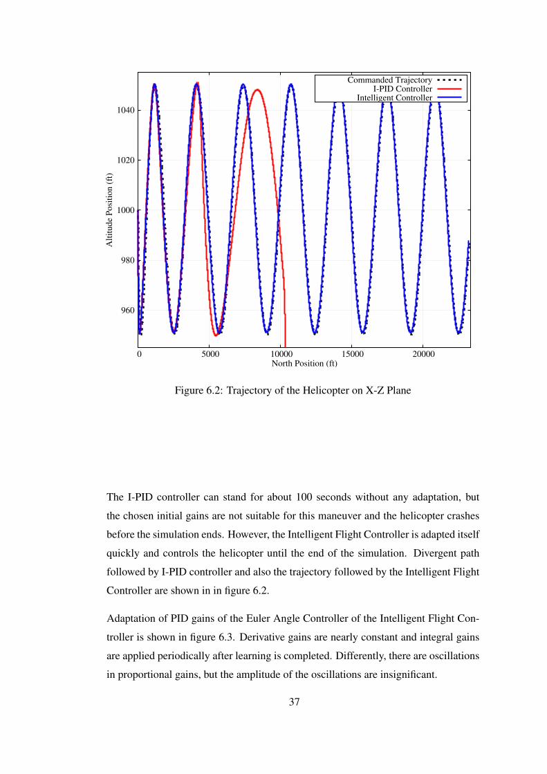
Figure 6.4: Adaptation History of the Body Angular Velocity Controller Gains

Learning regime of PID gains of the Body Angular Velocity Controller of the Intel-

ligent Flight Controller is illustrated in figure 6.4. Proportional and derivative gains

have continuous oscillations with negligible amplitudes. As integral gains of the Euler

Angle Controller, integral gains of the Body Angular Velocity Controller are applied

periodically after learning is completed. Although integral gains seem unstable at the

beginning, the peak amplitude of the integral gains are not changed after adaptation

is completed.

The stability of the PID gains of the Body Angular Velocity Controller provides stable

PID gains for Euler Angle Controller as shown in figure 6.3.

39

0

0.1

0.2

0.3

0.4

0.5

0 50 100 150 200 250 300

Phi

RM

SE

(deg

)

time (s)

I-PIDIFC

0 2 4 6 8

10 12 14

0 50 100 150 200 250 300

Nort

h R

MS

E (

ft)

time (s)

I-PIDIFC

0 0.2 0.4 0.6 0.8

1 1.2 1.4

0 50 100 150 200 250 300

Thet

a R

MS

E (

deg

)

time (s)

I-PIDIFC

0

0.1

0.2

0.3

0.4

0.5

0 50 100 150 200 250 300E

ast

RM

SE

(ft

)time (s)

I-PIDIFC

0

0.1

0.2

0.3

0.4

0.5

0 50 100 150 200 250 300

Psi

RM

SE

(deg

)

time (s)

I-PIDIFC

0

0.1

0.2

0.3

0.4

0.5

0 50 100 150 200 250 300

Alt

itude

RM

SE

(ft

)

time (s)

I-PIDIFC

Figure 6.5: RMSE Analyses of the Positions of the Helicopter in Pull Up - Push Over

Maneuver

When comparing the root mean square errors of six positions for both controllers

from figure 6.5, effectiveness of the Intelligent Flight Controller is seen obviously

for all positions. In addition to the root mean square error analysis, it is seen from

in figure 6.6 that the Intelligent Flight Controller completes the given mission with

periodic but stable control inputs.

In consequence, the reference trajectory for pull up - push over maneuver is followed

successfully by the Intelligent Flight Controller. However, I-PID controller with fixed

gains lose the control and helicopter hit the ground within 150 seconds. Therefore,

simulation for I-PID controller is stopped at 150th second as it can be seen on figure

6.6.

40

-10-8-6-4-2 0 2 4 6 8

10

0 50 100 150 200 250 300

Lon

git

ud

inal

Cycl

ic (

deg

)

time (s)

I-PIDIFC

-10

-5

0

5

10

15

20

25

0 50 100 150 200 250 300

Lat

eral

Cy

clic

(d

eg)

time (s)

I-PIDIFC

10 11 12 13 14 15 16 17 18 19 20 21

0 50 100 150 200 250 300

Coll

ecti

ve

(deg

)

time (s)

I-PIDIFC

9.9 9.92 9.94 9.96 9.98

10 10.02 10.04 10.06 10.08

0 50 100 150 200 250 300

Ped

al (

deg

)

time (s)

I-PIDIFC

Figure 6.6: Control Inputs Generated by I-PID and IFC in Pull Up - Push Over Ma-

neuver

6.2.2 Slalom Maneuver

The lateral channel of the flight controller is tested in the slalom maneuver for 300

seconds. A sinusoidal 100 ft peak-peak east position change within 100 seconds time

41

period and a constant 10 knots north velocity are expected in this maneuver [16].


commanded position equations for slalom maneuver,

XN =

∫VN dt (6.10)

XE = A

∫sin(

2π

TXN) dt (6.11)

XD = −1000 (6.12)

ψ = 0 (6.13)

where A=50 ft, T=100 seconds and VN=10 knots.

0

1000

2000

3000

4000

5000

-40 -20 0 20 40

Nort

h P

osi

tion (

ft)

East Position (ft)



Figure 6.7: Trajectory of the Helicopter on X-Y Plane

42

The I-PID controller can follow the desired trajectory with oscillations for about 250

seconds without any adaptation. However, these oscillations continuously increases

due to the incorrect initial gains for this maneuver and the helicopter crashes before

end of the simulation. The process which leads to crash is seen obviously from the

controller inputs in figure 6.11.

Unlike I-PID controller, the Intelligent Flight Controller completes the learning within

50 seconds and completes this test successfully. Divergence of the path followed by

I-PID controller and also the effort of the Intelligent Flight Controller are shown in

figure 6.7.

9.8 9.85 9.9

9.95 10

10.05 10.1

10.15 10.2

10.25

0 50 100 150 200 250 300

P G

ain

time (s)

PhiTheta

Psi

0 0.05 0.1

0.15 0.2

0.25 0.3

0.35 0.4

0 50 100 150 200 250 300

I G

ain

time (s)

PhiTheta

Psi

4.6

4.7

4.8

4.9

5

5.1

5.2

0 50 100 150 200 250 300

D G

ain

time (s)

PhiTheta

Psi



troller is shown in figure 6.8. Proportional and derivative gains are nearly constant

and integral gains are applied periodically with a very low frequency and insignificant

amplitude after learning is completed.

43

Initial short-time peaks with small amplitudes for integral and derivative gains of theta

and psi channels are related with the adaptation process and transition from hover to

forward flight. As helicopter reaches to 10 knots forward speed, these peaks fade out

due to the completion of adaptation.

The stability of the PID gains of the Euler Angle Controller of the Intelligent Flight

Controller provides an accurate trajectory as shown in figure 6.7.

16 18 20 22 24 26 28 30 32

0 50 100 150 200 250 300

P G

ain

time (s)

pqr

0 1 2 3 4 5 6 7 8 9

10

0 50 100 150 200 250 300

I G

ain

time (s)

pqr

4 6 8

10 12 14 16 18 20 22 24

0 50 100 150 200 250 300

D G

ain

time (s)

pqr


PID gains of the Body Angular Velocity Controller of the Intelligent Flight Controller

are also stable and depicted in figure 6.9. After learning process is completed, propor-

tional and derivative gains are nearly constant until the end of the simulation. Integral

gains of p and q channels of the Body Angular Velocity Controller are also constant.

However, integral gain of r channel is applied periodically with a very low frequency

after learning is completed. Because of very low frequency, integral gain of r channel

does not cause an unexpected disturbance for 300 seconds.

44

The stability of the PID gains of the Body Angular Velocity Controller provides stable

PID gains for Euler Angle Controller as shown in figure 6.8.

0

0.2

0.4

0.6

0.8

1

0 50 100 150 200 250 300

Phi

RM

SE

(deg

)

time (s)

I-PIDIFC

0

2

4

6

8

10

0 50 100 150 200 250 300

Nort

h R

MS

E (

ft)

time (s)

I-PIDIFC

0

0.2

0.4

0.6

0.8

1

0 50 100 150 200 250 300

Thet

a R

MS

E (

deg

)

time (s)

I-PIDIFC

0

1

2

3

4

5

0 50 100 150 200 250 300E

ast

RM

SE

(ft

)time (s)

I-PIDIFC

0

0.2

0.4

0.6

0.8

1

0 50 100 150 200 250 300

Psi

RM

SE

(deg

)

time (s)

I-PIDIFC

0

1

2

3

4

5

0 50 100 150 200 250 300

Alt

itude

RM

SE

(ft

)

time (s)

I-PIDIFC

Figure 6.10: RMSE Analyses of the Positions of the Helicopter in Slalom Maneuver

The root mean square errors of six positions for both controllers as shown in figure

6.10 indicate the effectiveness of the Intelligent Flight Controller for all positions. It

is also seen in figure 6.10 that I-PID controller with constant gains lose control in

all positions after 250 seconds. In addition to the root mean square error analysis, it

is seen from in figure 6.11 that the Intelligent Flight Controller completes the given

mission with nearly constant control inputs. However, control deflections of the I-PID

controller with fixed gains oscillate increasingly.

Consequently, the reference desired trajectory for slalom maneuver is accomplished

by the Intelligent Flight Controller without any bias. However, I-PID controller with

fixed gains cannot control the helicopter and helicopter crashes after about 250 sec-

onds as it can be seen on figure 6.7.

45

-4

-2

0

2

4

6

8

10

0 50 100 150 200 250 300

Lon

git

ud

inal

Cycl

ic (

deg

)

time (s)

I-PIDIFC

-10

-5

0

5

10

15

20

25

0 50 100 150 200 250 300

Lat

eral

Cy

clic

(d

eg)

time (s)

I-PIDIFC

-5

0

5

10

15

20

25

0 50 100 150 200 250 300

Coll

ecti

ve

(deg

)

time (s)

I-PIDIFC

9.9

9.92

9.94

9.96

9.98

10

10.02

10.04

0 50 100 150 200 250 300

Ped

al (

deg

)

time (s)

I-PIDIFC

Figure 6.11: Control Inputs Generated by I-PID and IFC in Slalom Maneuver

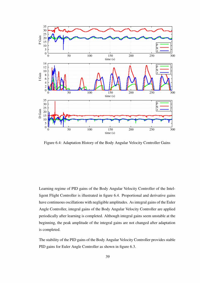
6.2.3 Pull Up - Push Over - Slalom Maneuver

This maneuver is a combination of pull up - push over and slalom maneuvers. Both

lateral and longitudinal channels of the flight controller are tested in pull up - push

over - slalom maneuver for 300 seconds. A sinusoidal 100 ft peak-peak east position

46

change within 100 seconds time period and a sinusoidal 100 ft peak-peak altitude

change within 50 seconds time period are expected in this maneuver. The forward

velocity target is 50 knots constant during flight.


commanded position equations for slalom maneuver,

XN =

∫VN dt (6.14)

XE = A

∫sin(

2π

T1XN) dt (6.15)

XD = −1000− A∫sin(

2 π

T2XN) dt (6.16)

ψ = 0 (6.17)

where A=50 ft, T1=100 seconds, T2=50 seconds and VN=50 knots.

47

0

5000

10000

15000

20000

-40 -20 0 20 40

Nort

h (

ft)

East (ft)




At the end of the simulation, the I-PID controller cannot follow the reference trajec-

tory and the helicopter crashes after about 120 seconds. Although I-PID controller

can follow the North-Altitude trajectory for about 60 seconds as seen in figure 6.13,

due to the unstable characteristics of the helicopter in lateral channel as shown in fig-

ure 6.12, initial gains are not enough to control in lateral channel and attitude of the

helicopter crashes with I-PID controller.

The process of crash is seen obviously from growing oscillations in the longitudinal

cyclic, lateral cyclic and collective controls as shown in figure 6.17. These oscillations

are started after about 30 seconds for longitudinal cyclic, lateral cyclic and collective

controls and lead to crash of the helicopter after about 120 seconds.

48

960

980

1000

1020

1040

0 5000 10000 15000 20000

Alt

itude

Posi

tion (

ft)

North Position (ft)



Figure 6.13: Trajectory of the Helicopter on X-Z Plane

However, the Intelligent Flight Controller is adapted itself within the first 20 seconds

and maintains the control of the helicopter for 300 seconds as shown in figures 6.12

and 6.13. Thus, the helicopter follows correct trajectories for both North-Altitude and

North-East channels with the Intelligent Flight Controller.


troller is shown in figure 6.14. Compulsion of the Intelligent Flight Controller is un-

derstood from the oscillations of PID gains. Derivative gains are more stable. Integral

gains are applied periodically even after learning is completed. Although the oscilla-

tions in proportional gains shows an unstable regime, the amplitude of the oscillations

are small in magnitude and they cannot force the Intelligent Flight Controller to lead

a crash during the simulation period.

49

9.8

9.85

9.9

9.95

10

10.05

10.1

10.15

0 50 100 150 200 250 300

P G

ain

time (s)

PhiTheta

Psi

0

0.1

0.2

0.3

0.4

0.5

0.6

0 50 100 150 200 250 300

I G

ain

time (s)

PhiTheta

Psi

4.6

4.7

4.8

4.9

5

5.1

5.2

0 50 100 150 200 250 300

D G

ain

time (s)

PhiTheta

Psi


The amplitude of oscillations in proportional channel for theta control is larger than

other channels. This difference is expected since the maneuver challenges the longi-

tudinal stability of the controller directly by pull up - push over maneuver. In addi-

tion, minor oscillations are existed in phi and psi channels due to the difficulty of the

slalom maneuver. These oscillations of the PID gains of the Euler Angle Controller

cannot deter the Intelligent Flight Controller to follow correct trajectories for both

North-Altitude and North-East channels as seen in figures 6.12 and 6.13.

Initial short-time peaks with small amplitudes for integral and derivative gains of

theta and psi channels also occur in this maneuver. As helicopter reaches to 50 knots

forward speed, adaptation gets easier and these peaks are fade out.

50

12 14 16 18 20 22 24 26 28 30 32 34

0 50 100 150 200 250 300

P G

ain

time (s)

pqr

0 2 4 6 8

10 12 14 16 18

0 50 100 150 200 250 300

I G

ain

time (s)

pqr

0

5

10

15

20

25

30

0 50 100 150 200 250 300

D G

ain

time (s)

pqr


Learning process of PID gains of the Body Angular Velocity Controller of the In-

telligent Flight Controller is shown in figure 6.15. Proportional and derivative gains

behave sinusoidally with small magnitudes. As integral gains of the Euler Angle Con-

troller, integral gains of the Body Angular Velocity Controller are applied periodically

after learning is completed except integral gain of r controller. Between about 140th

and 265th seconds, integral gain of r controller suddenly increases and then fades out.

These gain oscillations show the complexity of this maneuver. In spite of this com-

plexity, the Intelligent Flight Controller can control the helicopter until the end of the

simulation and follows the desired trajectory.

51

0

0.2

0.4

0.6

0.8

1

0 50 100 150 200 250 300

Phi

RM

SE

(deg

)

time (s)

I-PIDIFC

0 2 4 6 8

10 12 14

0 50 100 150 200 250 300

Nort

h R

MS

E (

ft)

time (s)

I-PIDIFC

0 0.2 0.4 0.6 0.8

1 1.2 1.4

0 50 100 150 200 250 300

Thet

a R

MS

E (

deg

)

time (s)

I-PIDIFC

0

1

2

3

4

5

0 50 100 150 200 250 300E

ast

RM

SE

(ft

)time (s)

I-PIDIFC

0

0.2

0.4

0.6

0.8

1

0 50 100 150 200 250 300

Psi

RM

SE

(deg

)

time (s)

I-PIDIFC

0

1

2

3

4

5

0 50 100 150 200 250 300

Alt

itude

RM

SE

(ft

)

time (s)

I-PIDIFC

Figure 6.16: RMSE Analyses of the Positions of the Helicopter in Pull Up - Push

Over - Slalom Maneuver

Root mean square errors of six positions for both controllers from figure 6.16 show

the effectiveness of the Intelligent Flight Controller for all positions. According to

RMSE analysis, I-PID controller lose the control of the helicopter nearly at the be-

ginning. But, the Intelligent Flight Controller maintains the control until the end of

the simulation. In addition to the root mean square error analysis, it is shown in fig-

ure 6.17 that the Intelligent Flight Controller accomplishes the given mission with

periodic but stable control inputs.

To sum up, the reference trajectory for the pull up - push over - slalom maneuver is

followed successfully by the Intelligent Flight Controller. However, I-PID controller

with constant gains lose the control and thus the helicopter hit the ground within 100

seconds.

52

-6

-4

-2

0

2

4

6

8

10

0 50 100 150 200 250 300

Lon

git

ud

inal

Cycl

ic (

deg

)

time (s)

I-PIDIFC

-10

-5

0

5

10

15

20

25

0 50 100 150 200 250 300

Lat

eral

Cy

clic

(d

eg)

time (s)

I-PIDIFC

8

10

12

14

16

18

20

22

0 50 100 150 200 250 300

Coll

ecti

ve

(deg

)

time (s)

I-PIDIFC

9.85

9.9

9.95

10

10.05

10.1

10.15

0 50 100 150 200 250 300

Ped

al (

deg

)

time (s)

I-PIDIFC

Figure 6.17: Control Inputs Generated by I-PID and IFC in Pull Up - Push Over -

Slalom Maneuver

6.2.4 Coning Maneuver

Both lateral and longitudinal channels of the flight controller are tested in the coning

maneuver in the case of a constant heading change. A continuously rounding path

53

with a decreasing radius is expected along north and east positions like drawing a

cone in the case of a constant heading change. Total velocity is 8 knots and heading

rate is 4.58 deg/s during flight. [16].


commanded position equations for coning maneuver,

XN =

∫VTotal sin

(∫ψ dt

)dt (6.18)

XE =

∫VTotal cos

(∫ψ dt

)dt (6.19)

XD = −1000 (6.20)

ψ =VTotalR

(6.21)

where R=100 ft and VTotal=8 knots.

54

0

100

200

300

400

500

600

700

0 100 200 300 400 500 600 700

Nort

h P

osi

tion (

ft)

East Position (ft)




This maneuver is hard to accomplish due to the constant heading rate and continu-

ously decreasing radius of the trajectory. Therefore, the simulation is limited to 120

seconds for both controllers. At the beginning, helicopter accelerates to reach 8 knots

to start to draw a cone. The Intelligent Flight Controller reaches to 8 knots in to-

tal velocity and follows the trajectory as expected. The Intelligent Flight Controller

completes two loops in this maneuver.

However, the I-PID controller cannot start to draw a cone due to the incorrect gains

for this maneuver. In spite of following the same trajectory with the Intelligent Flight

Controller for about 10 seconds, the I-PID controller leaves the path within 60 sec-

onds as seen in figure 6.18.

55

9.6

9.7

9.8

9.9

10

10.1

10.2

10.3

0 20 40 60 80 100 120

P G

ain

time (s)

PhiTheta

Psi

0 0.1 0.2 0.3 0.4 0.5 0.6 0.7 0.8

0 20 40 60 80 100 120

I G

ain

time (s)

PhiTheta

Psi

4.5

4.6

4.7

4.8

4.9

5

5.1

5.2

0 20 40 60 80 100 120

D G

ain

time (s)

PhiTheta

Psi


Adaptation process of PID gains of the Euler Angle Controller of the Intelligent Flight

Controller is shown in figure 6.19. Because of the complexity of the coning maneu-

ver, PID gains of the Euler Angle Controller are not as smooth as in the previous

maneuvers.

There are sinusoidal oscillations for all gains, but the amplitude of these oscillations

are small. In spite of the oscillations, the Intelligent Flight Controller can follow the

desired trajectory in this maneuver. The most oscillatory gains of the Euler Angle

Controller are belonged to psi controller because of the constant heading rate and

continuously decreasing radius of the trajectory of the coning maneuver.

56

5

10

15

20

25

30

35

0 20 40 60 80 100 120

P G

ain

time (s)

pqr

0 2 4 6 8

10 12 14 16

0 20 40 60 80 100 120

I G

ain

time (s)

pqr

0

5

10

15

20

25

0 20 40 60 80 100 120

D G

ain

time (s)

pqr


Learning process of PID gains of the Body Angular Velocity Controller of the Intel-

ligent Flight Controller is illustrated in figure 6.20. Proportional and derivative gains

have continuous oscillations with small amplitudes. As integral gains of the Euler

Angle Controller, integral gains of the Body Angular Velocity Controller are applied

periodically after learning is completed.

As in the Euler Angle Controller, the most oscillatory gains of the Body Angular

Velocity Controller are belonged to psi controller because of the constant heading

rate and continuously decreasing radius of the trajectory of the coning maneuver.

In spite of these oscillations, the Intelligent Flight Controller can control the heli-

copter until the end of the simulation and follows the desired trajectory.

57

0

0.1

0.2

0.3

0.4

0.5

0 20 40 60 80 100 120

Phi

RM

SE

(deg

)

time (s)

I-PIDIFC

0

1

2

3

4

5

0 20 40 60 80 100 120

Nort

h R

MS

E (

ft)

time (s)

I-PIDIFC

0

0.1

0.2

0.3

0.4

0.5

0 20 40 60 80 100 120

Thet

a R

MS

E (

deg

)

time (s)

I-PIDIFC

0

1

2

3

4

5

0 20 40 60 80 100 120E

ast

RM

SE

(ft

)time (s)

I-PIDIFC

0

0.1

0.2

0.3

0.4

0.5

0 20 40 60 80 100 120

Psi

RM

SE

(deg

)

time (s)

I-PIDIFC

0

1

2

3

4

5

0 20 40 60 80 100 120

Alt

itude

RM

SE

(ft

)

time (s)

I-PIDIFC

Figure 6.21: RMSE Analyses of the Positions of the Helicopter in Coning Maneuver

Root mean square error analyses of six positions for both controllers from figure 6.21

show the effectiveness of the Intelligent Flight Controller for all positions. Accord-

ing to RMSE analysis, the trajectory followed by I-PID controller diverges from the

reference nearly at the beginning. But, the Intelligent Flight Controller maintains the

tacking the reference trajectory until the end of the simulation. In addition to the

root mean square error analysis, it is shown in figure 6.22 that the Intelligent Flight

Controller accomplishes the given mission with nearly constant control inputs.

In consequence, the reference trajectory for coning maneuver is followed successfully

by the Intelligent Flight Controller. However, I-PID controller with fixed gains cannot

start to draw a cone and follows a different path rather than the reference trajectory as

seen on figure 6.18.

58

-6

-4

-2

0

2

4

6

8

10

0 20 40 60 80 100 120

Lon

git

ud

inal

Cycl

ic (

deg

)

time (s)

I-PIDIFC

-10

-5

0

5

10

15

20

25

0 20 40 60 80 100 120

Lat

eral

Cy

clic

(d

eg)

time (s)

I-PIDIFC

12 13 14 15 16 17 18 19 20 21

0 20 40 60 80 100 120

Coll

ecti

ve

(deg

)

time (s)

I-PIDIFC

9.92

9.94

9.96

9.98

10

10.02

10.04

10.06

10.08

0 20 40 60 80 100 120

Ped

al (

deg

)

time (s)

I-PIDIFC

Figure 6.22: Control Inputs Generated by I-PID and IFC in Coning Maneuver

6.2.5 Pirouette Maneuver

Both lateral and longitudinal channels of the flight controller are tested in the pirouette

maneuver in the case of a constant heading change. A continuously rounding path

with a decreasing radius is expected along north and east positions. But, in this case

59

heading rate is faster and constant north velocity is slower than coning maneuver.

Hence, this condition causes to turn around a single point which is the definition of

pirouette. 6.88 deg/s yaw rate in reverse direction and a constant 6 knots total velocity

are expected in this maneuver [16].


commanded position equations for pirouette maneuver,

XN =

∫VTotal sin

(∫ψ dt

)dt (6.22)

XE =

∫VTotal cos

(∫ψ dt

)dt (6.23)

XD = −1000 (6.24)

ψ = −2VTotalR

(6.25)


60

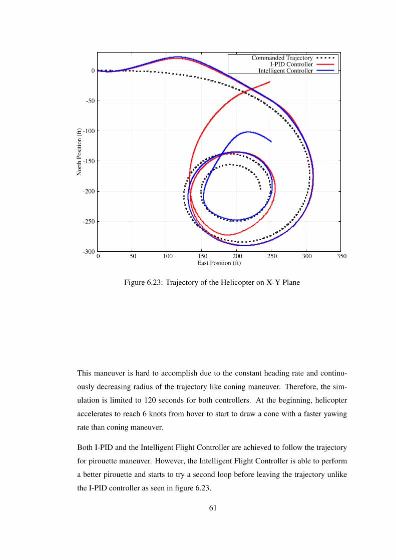
-300

-250

-200

-150

-100

-50

0

0 50 100 150 200 250 300 350

Nort

h P

osi

tion (

ft)

East Position (ft)




This maneuver is hard to accomplish due to the constant heading rate and continu-

ously decreasing radius of the trajectory like coning maneuver. Therefore, the sim-

ulation is limited to 120 seconds for both controllers. At the beginning, helicopter

accelerates to reach 6 knots from hover to start to draw a cone with a faster yawing

rate than coning maneuver.

Both I-PID and the Intelligent Flight Controller are achieved to follow the trajectory

for pirouette maneuver. However, the Intelligent Flight Controller is able to perform

a better pirouette and starts to try a second loop before leaving the trajectory unlike

the I-PID controller as seen in figure 6.23.

61

9.75 9.8

9.85 9.9

9.95 10

10.05 10.1

10.15 10.2

10.25

0 20 40 60 80 100 120

P G

ain

time (s)

PhiTheta

Psi

0

0.1

0.2

0.3

0.4

0.5

0.6

0 20 40 60 80 100 120

I G

ain

time (s)

PhiTheta

Psi

4.5

4.6

4.7

4.8

4.9

5

5.1

5.2

0 20 40 60 80 100 120

D G

ain

time (s)

PhiTheta

Psi


Learning process of PID gains of the Euler Angle Controller of the Intelligent Flight

Controller is depicted in figure 6.24. Because of the complexity of the pirouette

maneuver, PID gains of the Euler Angle Controller are not as smooth as in the pull

up - push over and slalom maneuvers.

There are sinusoidal oscillations for all gains, but the amplitude of these oscillations

are small. In addition, there are short-time small peaks for derivative gains. In spite

of the oscillations and small peaks, the Intelligent Flight Controller can follow the

desired trajectory in this maneuver. As in the coning maneuver, the most oscillatory

gains of the Euler Angle Controller are the psi controller gains because of the con-

stant heading rate and continuously decreasing radius of the trajectory of the pirouette

maneuver.

62

12 14 16 18 20 22 24 26 28 30 32 34

0 20 40 60 80 100 120

P G

ain

time (s)

pqr

0

5

10

15

20

25

0 20 40 60 80 100 120

I G

ain

time (s)

pqr

2 4 6 8

10 12 14 16 18 20 22 24

0 20 40 60 80 100 120

D G

ain

time (s)

pqr


Adaptation process of PID gains of the Body Angular Velocity Controller of the Intel-

ligent Flight Controller is shown in figure 6.25. Proportional, derivative and integral

gains have continuous oscillations with small amplitudes and short-time small peaks

except r controller.

Amplitudes of peaks in derivative gain, amplitudes of oscillations in proportional and

integral gains of r controller are not so small because of the constant heading rate and

continuously decreasing radius of the trajectory of the pirouette maneuver.

In spite of these oscillations and peaks, the Intelligent Flight Controller can control

the helicopter until the end of the simulation and follows the desired trajectory.

63

0

0.1

0.2

0.3

0.4

0.5

0 20 40 60 80 100 120

Phi

RM

SE

(deg

)

time (s)

I-PIDIFC

0

1

2

3

4

5

0 20 40 60 80 100 120

Nort

h R

MS

E (

ft)

time (s)

I-PIDIFC

0

0.1

0.2

0.3

0.4

0.5

0 20 40 60 80 100 120

Thet

a R

MS

E (

deg

)

time (s)

I-PIDIFC

0

1

2

3

4

5

0 20 40 60 80 100 120E

ast

RM

SE

(ft

)time (s)

I-PIDIFC

0

0.1

0.2

0.3

0.4

0.5

0 20 40 60 80 100 120

Psi

RM

SE

(deg

)

time (s)

I-PIDIFC

0

1

2

3

4

5

0 20 40 60 80 100 120

Alt

itude

RM

SE

(ft

)

time (s)

I-PIDIFC

Figure 6.26: RMSE Analyses of the Positions of the Helicopter in Pirouette Maneuver

As it is shown in figure 6.26, root mean square error analyses of six positions for

both controllers are similar until the last 20 seconds. The Intelligent Flight Controller

is still more effective for all positions. According to RMSE analysis, the trajectory

followed by I-PID controller diverges from the reference in the last 20 seconds. But,

the Intelligent Flight Controller maintains to track the reference trajectory until the

end of the simulation. In addition to the root mean square error analysis, it is shown

in figure 6.27 that the Intelligent Flight Controller completes the given mission with

more stable control inputs.

In conclusion, the Intelligent Flight Controller is more successful for following the

desired trajectory than the I-PID controller with fixed gains in pirouette maneuver as

seen on figure 6.23.

64

-6

-5

-4

-3

-2

-1

0

1

2

0 20 40 60 80 100 120

Lon

git

ud

inal

Cycl

ic (

deg

)

time (s)

I-PIDIFC

6 6.5

7 7.5

8 8.5

9 9.5 10

10.5

0 20 40 60 80 100 120

Lat

eral

Cy

clic

(d

eg)

time (s)

I-PIDIFC

13.25 13.3

13.35 13.4

13.45 13.5

13.55 13.6

13.65 13.7

13.75

0 20 40 60 80 100 120

Coll

ecti

ve

(deg

)

time (s)

I-PIDIFC

9.88 9.9

9.92 9.94 9.96 9.98

10 10.02 10.04 10.06 10.08

0 20 40 60 80 100 120

Ped

al (

deg

)

time (s)

I-PIDIFC

Figure 6.27: Control Inputs Generated by I-PID and IFC in Pirouette Maneuver

6.2.6 3-D Cone Maneuver

The last maneuver is the combination of all maneuvers to challenge the flight con-

troller as much as possible. A continuously rounding path with a decreasing radius

like drawing a cone is expected for all positions. 3.44 deg/s yaw rate and a constant

65

3 knots total velocity are expected in this maneuver. At the beginning, the maneuver

is much simpler for flight controllers. But, as the radius of the cone decreases, path

tracking becomes increasingly challenging due to the constant heading rate.


commanded position equations for 3-D Cone maneuver,

XN =

∫VTotal sin

(∫ψ dt

)dt+

∫ ∣∣∣sin(∫ ψ dt)∣∣∣ dt (6.26)

XE =

∫VTotal cos

(∫ψ dt

)dt (6.27)

XD = −1000 +

∫VTotal sin

(∫ψ dt

)dt (6.28)

ψ = 2VTotalR

(6.29)


66

150

200

250

300

350

80 100 120 140 160 180 200 220

Nort

h P

osi

tion (

ft)

East Position (ft)




As the simulation continues, completion of the loops in this maneuver gets harder an

harder for both controllers due to the constant heading rate and continuously decreas-

ing radius of the trajectory like coning maneuver. Unlike the coning and pirouette

maneuvers, the simulation is conducted for 300 seconds for this maneuver because

of the slower total velocity. At the beginning, helicopter accelerates to reach 3 knots

from hover to start to draw a 3-D cone with a constant yaw rate.

Both I-PID and the Intelligent Flight Controller are able to follow the trajectory for

3-D cone maneuver until the last 40 seconds. In the last 40 seconds of the simulation,

I-PID controller leaves the trajectory as seen in figure 6.28. However, the Intelligent

Flight Controller continues to complete loops for this maneuver.

67

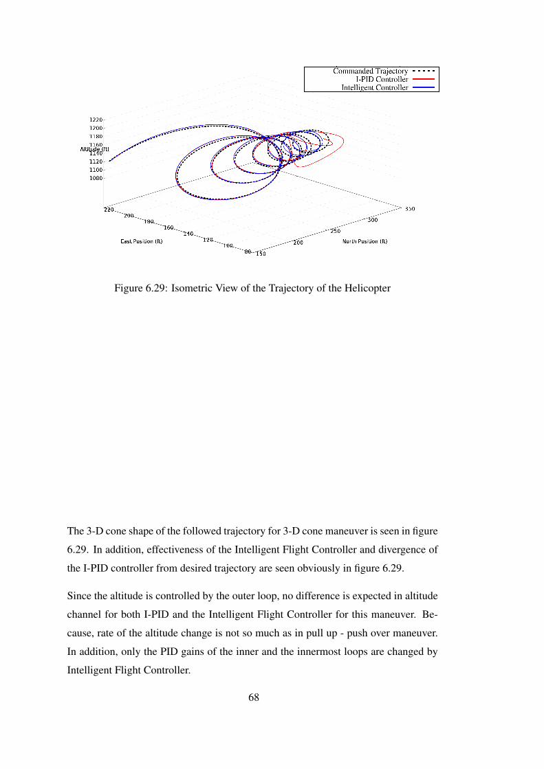
Figure 6.29: Isometric View of the Trajectory of the Helicopter

The 3-D cone shape of the followed trajectory for 3-D cone maneuver is seen in figure

6.29. In addition, effectiveness of the Intelligent Flight Controller and divergence of

the I-PID controller from desired trajectory are seen obviously in figure 6.29.

Since the altitude is controlled by the outer loop, no difference is expected in altitude

channel for both I-PID and the Intelligent Flight Controller for this maneuver. Be-

cause, rate of the altitude change is not so much as in pull up - push over maneuver.

In addition, only the PID gains of the inner and the innermost loops are changed by

Intelligent Flight Controller.

68

9.7 9.75 9.8

9.85 9.9

9.95 10

10.05 10.1

10.15 10.2

0 50 100 150 200 250 300

P G

ain

time (s)

PhiTheta

Psi

0

0.1

0.2

0.3

0.4

0.5

0.6

0 50 100 150 200 250 300

I G

ain

time (s)

PhiTheta

Psi

4.6 4.65 4.7

4.75 4.8

4.85 4.9

4.95 5

5.05 5.1

0 50 100 150 200 250 300

D G

ain

time (s)

PhiTheta

Psi


Learning process of PID gains of the Euler Angle Controller of the Intelligent Flight

Controller is depicted in figure 6.30. Because of the complexity of the 3-D cone

maneuver, PID gains of the Euler Angle Controller are oscillatory as in coning and

piroutte maneuvers.

The amplitude of the PID gain oscillations are small in magnitude. In addition, there

are short-time small peaks for derivative gains. In spite of the oscillations and small

peaks, the Intelligent Flight Controller can follow the desired trajectory better than

I-PID controller in this maneuver. As in the coning and piroutte maneuvers, the most

oscillatory gains of the Euler Angle Controller are the psi controller gains because of

the constant heading rate and continuously decreasing radius of the trajectory of the

3-D cone maneuver.

69

14 16 18 20 22 24 26 28 30 32

0 50 100 150 200 250 300

P G

ain

time (s)

pqr

0 1 2 3 4 5 6 7 8 9

0 50 100 150 200 250 300

I G

ain

time (s)

pqr

2 4 6 8

10 12 14 16 18

0 50 100 150 200 250 300

D G

ain

time (s)

pqr


Adaptation process of PID gains of the Body Angular Velocity Controller of the In-

telligent Flight Controller is shown in figure 6.31. Proportional and derivative gains

are nearly constant. In addition derivative gains have small short-time peaks and there

are periodic oscillations with small amplitudes in integral gains of p and q controllers.

Amplitudes of peaks in derivative gains, amplitudes of oscillations in proportional

and integral gains of r controller are not so small because of the constant heading rate

and continuously decreasing radius of the trajectory of the 3-D cone maneuver.

Although existence of these oscillations and peaks, the Intelligent Flight Controller

can control the helicopter better than the I-PID controller for 3-D cone maneuver.

70

0

0.05

0.1

0.15

0.2

0.25

0.3

0 50 100 150 200 250 300

Phi

RM

SE

(deg

)

time (s)

I-PIDIFC

0 0.2 0.4 0.6 0.8

1 1.2 1.4

0 50 100 150 200 250 300

Nort

h R

MS

E (

ft)

time (s)

I-PIDIFC

0

0.05

0.1

0.15

0.2

0.25

0.3

0 50 100 150 200 250 300

Thet

a R

MS

E (

deg

)

time (s)

I-PIDIFC

0 0.2 0.4 0.6 0.8

1 1.2 1.4

0 50 100 150 200 250 300

Eas

t R

MS

E (

ft)

time (s)

I-PIDIFC

0

0.05

0.1

0.15

0.2

0.25

0.3

0 50 100 150 200 250 300

Psi

RM

SE

(deg

)

time (s)

I-PIDIFC

0 0.2 0.4 0.6 0.8

1 1.2 1.4

0 50 100 150 200 250 300

Alt

itude

RM

SE

(ft

)

time (s)

I-PIDIFC

Figure 6.32: RMSE Analyses of the Positions of the Helicopter in 3-D Cone Maneu-

ver

As it is shown in figure 6.32, root mean square error analyses of six positions for

both controllers are similar until the last 40 seconds. The Intelligent Flight Controller

is still more effective for all positions. According to RMSE analysis, the trajectory

followed by I-PID controller diverges from the reference in the last 40 seconds. How-

ever, the Intelligent Flight Controller maintains to follow the reference trajectory until

the end of the simulation. In addition to the RMSE analysis, it is shown in figure 6.33

that the IFC completes the given mission with more stable control inputs.

To sum up, the IFC is more successful for following the desired trajectory than the

I-PID controller with fixed gains in 3-D cone maneuver as seen on figure 6.28.

71

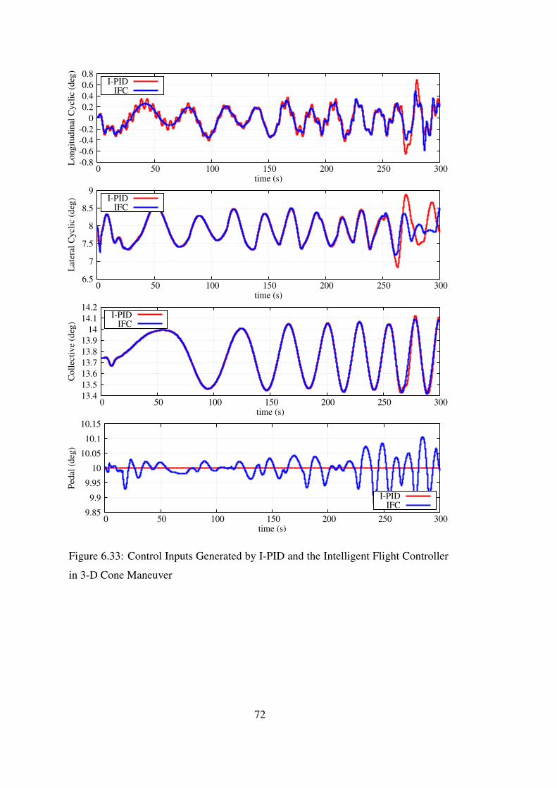
-0.8

-0.6

-0.4

-0.2

0

0.2

0.4

0.6

0.8

0 50 100 150 200 250 300

Lon

git

ud

inal

Cycl

ic (

deg

)

time (s)

I-PIDIFC

6.5

7

7.5

8

8.5

9

0 50 100 150 200 250 300

Lat

eral

Cy

clic

(d

eg)

time (s)

I-PIDIFC

13.4

13.5

13.6

13.7

13.8

13.9

14

14.1

14.2

0 50 100 150 200 250 300

Coll

ecti

ve

(deg

)

time (s)

I-PIDIFC

9.85

9.9

9.95

10

10.05

10.1

10.15

0 50 100 150 200 250 300

Ped

al (

deg

)

time (s)

I-PIDIFC

Figure 6.33: Control Inputs Generated by I-PID and the Intelligent Flight Controller

in 3-D Cone Maneuver

72

CHAPTER 7

CONCLUSION

In this study, a new intelligent flight controller is developed with model prediction

and adaptation abilities for a full sized autonomous helicopter. Testing platform for

the intelligent controller is selected as the UH-1H helicopter. To achieve this, UH-1H

helicopter is converted to an unmanned platform in virtual environment by developing

a full flight controller for hover and forward flight conditions.

For a contribution to the literature, a PID gain update law using linear least squares

regression is proposed as a new adaptive control method. Moreover, future prediction

analysis are conducted for error dynamics of the closed loop system using recursive

linear least squares regression. These two concepts are combined with conventional

PID controller and an intelligent PID controller is acquired.

Excluding the velocity controllers, PID controllers of the flight controller are replaced

by the newly developed intelligent PID controller. Thus, a new intelligent flight con-

troller is obtained with model prediction and adaptation abilities for autonomous he-

licopters.

Finally, several complex maneuvers are conducted to challenge the intelligent flight

controller. The first flight controller that has no adaptation ability and the new intelli-

gent flight controller are tested with same initally stable PID gains to demonstrate the

effectiveness of the new intelligent flight controller.

All challenging maneuvers are completed successfully by the new Intelligent Flight

Controller (IFC). However, these complex maneuvers are too aggressive for the flight

controller with fixed PID gains. Therefore, most of the maneuvers are ended due to

73

crash of the helicopter with this flight controller although using the same initial PID

gains with IFC.

However, the new controller IFC is not more effective than a very well tuned PID. The

results of the comparison between IFC and a very well tuned PID is not given in this

study because of the difference in the success ratio of these methods is approximately

1-3%. As stated in the introduction section, tuning the gains of the PID controllers is

very hard in practice. Therefore, acquiring a very well tuned PID is not an easy pro-

cess without using any advanced techniques like adaptive control. The main objective

for an adaptive controller is to find the optimum PID gains while maximizing given

performance index. The new controller IFC achieves such objective while satisfying

constraints, even starting from a very rough initial PID gains.

To sum up, a new PID update law using Linear Least Squares Regression is proposed

for adaptation. Implementing the acceleration of the command, an I-PID controller is

obtained. This I-PID controller is converted to a new intelligent I-PID controller by

adding adaptation and prediction abilities using Linear Least Squares Regression and

Recursive Linear Least Squares Regression, respectively. On the other hand, a flight

controller with three control loops is developed using I-PID controllers to convert

UH-1H to an autonomous helicopter. Then, the I-PID controllers of the second and

third loops of this flight controller are replaced by newly developed intelligent I-PID

controllers. Consequently, an effective intelligent flight controller is acquired for

autonomous helicopters.

7.1 Future Work

Suggested improvements for this thesis are listed below,

• PID gain update law can be extended for Proportional Integral Derivative Ac-

celeration (PIDA) controllers.

• Damped Linear Least Squares regression can be used for gain optimization

using forgetting factors for back-stepping.

• Non-Linear Least Squares regression methods can be used for adaptation of

74

PID gains and prediction of the error.

• Controller can be challenged for more complex maneuvers.

• Initial PID gains can be selected from an unstable closed loop condition to

analyze the fidelity range of the intelligent flight controller.

• Different gain update rules can be applied for the same intelligent flight con-

troller.

75

REFERENCES

[1] Cai, G., Chen, B., Peng, K., Dong, M., and Lee, T., Industrial Electronics, IEEETransactions on 55 (2008) 3426.

[2] Azeem, S., Autonomous unmanned aerial vehicles, Technical report, TheGeorge Washington University, 2012.

[3] Beharrell, A., Converting an inexpensive rc helicopter into an autonomous ve-hicle, Master’s thesis, University Of Southampton, 2011.

[4] Haddal, C. C. and Gertler, J., Homeland security: Unmanned aerial vehicles andborder surveillance, Technical report, U.S. Congressional Research Service,2010, Retrieved from: http://nsarchive.gwu.edu/NSAEBB/NSAEBB527-Using-overhead-imagery-to-track-domestic-US-targets/documents/EBB-Doc24.pdf, Last Accessed: May 22, 2016.

[5] Nicas, J., Drones find fans among farmers, filmmakers, Re-trieved from: http://www.wsj.com/articles/, 2014, Article ID:SB10001424052702304732804579425342990070808, Last Accessed: May22, 2016.

[6] Autonomous drone developed for Fukushima reactors (11.06.2015). Retrievedfrom: http://www.bbc.com/news/blogs-news-from-elsewhere-33096077, LastAccessed: May 22, 2016.

[7] Zhang, L. et al., Advanced Science and Technology Letters 81 (2015) 69.

[8] Smith, R., Utilities turn to drones to inspect power lines and pipelines,Retrieved from: http://www.wsj.com/articles/utilities-turn-to-drones-to-inspect-power-lines-and-pipelines-1430881491, 2015, Last Accessed: May 22, 2016.

[9] Hedges, S. and O’Brien, T., Monitoring Elephant Populations and AssessingThreats (2012).

[10] Gasperini, D., Allemand, P., Delacourt, C., and Grandjean, P., InternationalJournal of Environmental Technology and Management 17 (2014) 1.

[11] Khaleghi, A. M. et al., Agent-based hardware-in-the-loop simulation foruav/ugv surveillance and crowd control system, in Proceedings of the 2013Winter Simulation Conference: Simulation: Making Decisions in a ComplexWorld, pages 1455–1466, IEEE Press, 2013.

77

[12] Lee, C., Lee, Y., and Teng, C., A novel robust pid controllers design by fuzzyneural network, in American Control Conference, 2002. Proceedings of the2002, volume 2, pages 1561–1566 vol.2, 2002.

[13] Ming-guang, Z., Xing-gui, W., and qiang Liu, M., Adaptive pid control basedon rbf neural network identification, in Tools with Artificial Intelligence, 2005.ICTAI 05. 17th IEEE International Conference on, pages 3 pp.–683, 2005.

[14] Zein-Sabatto, S. and Zheng, Y., Intelligent flight controllers for helicopter con-trol, in Neural Networks,1997., International Conference on, volume 2, pages617–621 vol.2, 1997.

[15] Sanchez, E. N., Becerra, H. M., and Velez, C. M., Information Sciences 177(2007) 1999 , Including Special Issue on Hybrid Intelligent Systems.

[16] Tarimci, O., Adaptive controller applications for rotary wing aircraft models ofvarying simulation fidelity, Master’s thesis, METU, 2009.

[17] Sadeghzadeh, I., Mehta, A., Zhang, Y., and Rabbath, C.-A., Fault-tolerant tra-jectory tracking control of a quadrotor helicopter using gain-scheduled pid andmodel reference adaptive control, in Annual Conference of the Prognostics andHealth Management Society, volume 2, 2011.

[18] Sahu, P. and Pradhan, S., Multi variable self tuning pid control of a twin rotormimo system, in Advanced Communication Control and Computing Technolo-gies (ICACCCT), 2014 International Conference on, pages 381–385, 2014.

[19] Gao, H., Liu, C., Guo, D., and Liu, J., Fuzzy adaptive pd control for quadrotorhelicopter, in Cyber Technology in Automation, Control, and Intelligent Systems(CYBER), 2015 IEEE International Conference on, pages 281–286, 2015.

[20] Brickwedde, A., Industry Applications, IEEE Transactions on IA-21 (1985)1154.

[21] Éric Poulin, Pomerleau, A., Desbiens, A., and Hodouin, D., Automatica 32(1996) 71 .

[22] Rad, A., Lo, W. L., and Tsang, K., Industrial Electronics, IEEE Transactions on44 (1997) 717.

[23] Mitsukura, Y., Yamamoto, T., and Kaneda, M., A design of self-tuning pidcontrollers using a genetic algorithm, in American Control Conference, 1999.Proceedings of the 1999, volume 2, pages 1361–1365 vol.2, 1999.

[24] Grassi, E., Tsakalis, K. S., Dash, S., Gaikwad, S., and Stein, G., Adaptive/self-tuning pid control by frequency loop-shaping, in Decision and Control, 2000.Proceedings of the 39th IEEE Conference on, volume 2, pages 1099–1101 vol.2,2000.

78

[25] Chen, J. and Cheng, Y.-C., Industrial & engineering chemistry research 43(2004) 5888.

[26] Yamamoto, T. and Shah, S., Design of a performance-adaptive pid controller,in Control Conference (ECC), 2007 European, pages 4799–4804, 2007.

[27] Wanfeng, S., Shengdun, Z., and Yajing, S., Adaptive pid controller based ononline lssvm identification, in Advanced Intelligent Mechatronics, 2008. AIM2008. IEEE/ASME International Conference on, pages 694–698, 2008.

[28] Zhao, J., Li, P., and song Wang, X., Intelligent pid controller design with adap-tive criterion adjustment via least squares support vector machine, in Controland Decision Conference, 2009. CCDC ’09. Chinese, pages 7–12, 2009.

[29] Wilson, A., Schultz, J., and Murphey, T., Automation Science and Engineering,IEEE Transactions on 12 (2015) 28.

[30] Tao, G., Adaptive Control Design and Analysis, Wiley, 2003.

[31] Bretscher, O., Linear Algebra with Applications, Printice Hall, 2001.

[32] Chowdhary, G. V., Concurrent Learning For Convergence In Adaptive ControlWithout Persistency Of Excitation, PhD thesis, Daniel Guggenheim School ofAerospace Engineering, Georgia Institute of Technology, 2010.

[33] Kim, K., Rao, P., and Burnworth, J. A., IEEE Transactions on Industry Appli-cations 46 (2010).

[34] Burger, M. and Repiský, J., Problems of linear least square regression, in ARSA,volume 1, pages 257–262, EDIS - Publishing Institution of the University ofZilina, 2012.

[35] Renze, John. "Outlier." From MathWorld–A Wolfram Web Resource, created byEric W. Weisstein. http://mathworld.wolfram.com/Outlier.html, Last Accessed:May 22, 2016.

[36] Prasad, J., Calise, A., Pei, Y., and Corban, J. E., Adaptive nonlinear controllersynthesis and flight test evaluation on an unmanned helicopter, in InternationalConference on Control Applications, volume 1, pages 137–142, IEEE, 1999.

[37] Official Website of Heli-Dyn: http://www.heli-dyn.com/Helidyn/Home.html,Last Accessed: May 22, 2016.

[38] Talbot, P. D. and Corliss, L. D., A mathematical force and moment model of auh-1h helicopter for flight dynamics simulations, Technical report, NASA, Pre-pared in Cooperation with USAAMRDL Moffett Field, Calif., 1977, DocumentID:19770024231,.

79

[39] Heffley, R. K. and Mnich, M. A., Minimum-complexity helicopter simu-lation math model, Technical report, NASA, Prepared for Army Researchand Technology Labs., Moffett Field, Calif., 1988, NASA-CR-177476, NAS1.26:177476, USAAVSCOM-TR-87-A-7.

[40] Peters, D. A., Boyd, D. D., and He, C. J., Journal of the American HelicopterSociety 34 (1989) 5.

[41] Yilmaz, D., Evaluation and comparison of helicopter simulation models withdifferent fidelities, Master’s thesis, METU, 2008.

[42] Yavrucuk, I., Tarimci, O., Katircioglu, M., Kubali, E., and Yilmaz, D., A newhelicopter simulation and analysis tool: Helidyn+, European Rotorcraft Forum,2010.

80

APPENDIX A

ROOT MEAN SQUARE ERROR ANALYSIS OF MANEUVERS

Figure A.1: RMSE Analysis of Maneuvers

81

development of an intelligent model …etd.lib.metu.edu.tr/upload/12619999/index.pdf · controller...

Documents