DEVELOPMENT OF APPLE WORKGROUP CLUSTER AND

PARALLEL COMPUTING FOR PHASE FIELD MODEL OF

MAGNETIC MATERIALS

A Thesis

by

YONGXIN HUANG

Submitted to the Office of Graduate Studies of

Texas A&M University

in partial fulfillment of the requirements for the degree of

MASTER OF SCIENCE

May 2009

Major Subject: Aerospace Engineering

DEVELOPMENT OF APPLE WORKGROUP CLUSTER AND

PARALLEL COMPUTING FOR PHASE FIELD MODEL OF

MAGNETIC MATERIALS

A Thesis

by

YONGXIN HUANG

Submitted to the Office of Graduate Studies of

Texas A&M University

in partial fulfillment of the requirements for the degree of

MASTER OF SCIENCE

Approved by:

Chair of Committee, Yongmei Jin

Committee Members, Raymundo Arroyave

Zoubeida Ounaies

Head of Department, Dimitris Lagoudas

May 2009

Major Subject: Aerospace Engineering

iii

ABSTRACT

Development of Apple Workgroup Cluster and Parallel Computing

for Phase Field Model of Magnetic Materials. (May 2009)

Yongxin Huang, B.S., University of Science and Technology of China

Chair of Advisory Committee: Dr. Yongmei Jin

Micromagnetic modeling numerically solves magnetization evolution equation to

process magnetic domain analysis, which helps to understand the macroscopic

magnetic properties of ferromagnets. To apply this method in simulation of

magnetostrictive ferromagnets, there exist two main challenges: the complicated micro-

elasticity due to the magnetostrictive strain, and very expensive computation mainly

caused by the calculation of long-range magnetostatic and elastic interactions. A

parallel computing for phase field model based on computer cluster is then developed

as a promising tool for domain analysis in magnetostrictive ferromagnetic materials.

We have successfully built an 8-node Apple workgroup cluster, deploying the

hardware system and configuring the software environment, as a platform for parallel

computation of phase field model of magnetic materials. Several testing programs have

been implemented to evaluate the performance of the cluster system, especially for the

application of parallel computation using MPI. The results show the cluster system can

iv

simultaneously support up to 32 processes for MPI program with high performance of

interprocess communication.

The parallel computations of phase field model of magnetic materials implemented by

a MPI program have been performed on the developed cluster system. The simulated

results of a single domain rotation in Terfenol-D crystals agree well with the theoretical

prediction. A further simulation including magnetic and elastic interaction among

multiple domains shows that we need take into account the interaction effects in order

to accurately characterize the magnetization processes in Terfenol-D. These simulation

examples suggest that the paralleling computation of the phase field model of magnetic

materials based on a powerful cluster system is a promising technology that meets the

need of domain analysis.

v

ACKNOWLEDGEMENTS

I would like to thank my advisor, Dr. Yongmei Jin, who introduced me into the field of

computational materials science. Dr. Jin helped me to broaden my knowledge of

mathematics, mechanics, and materials science. She always encouraged me to take any

challenge with a positive attitude.

I am very grateful to my committee members, Dr. Ounaies and Dr. Arroyave, for their

support.

I want to thank James Munnerlyn, Computer System Manager with the Aerospace

Engineering Department, for helping with the installation and maintenance of our

cluster system. I also thank Dr. Srinivasan for answering my questions which helped

me start the work on computer cluster.

Special thanks to my parents and my girlfriend.

vi

TABLE OF CONTENTS

Page

ABSTRACT ....................................................................................................................... iii

ACKNOWLEDGEMENTS ............................................................................................... v

TABLE OF CONTENTS ................................................................................................... vi

LIST OF FIGURES......................................................................................................... vii

1 INTRODUCTION............................................................................................................ 1

1.1 Magnetic microstructure analysis............................................................................ 1

1.2 Phase field model .................................................................................................... 4

1.3 Parallel computing................................................................................................... 8

1.4 Description of the thesis ........................................................................................ 12

2 BUILDING CLUSTER SYSTEM FOR PARALLEL COMPUTATION..................... 13

2.1 Overview of a computer cluster system ................................................................ 13

2.2 Hardware system structure .................................................................................... 15

2.2.1 Compute nodes .......................................................................................... 15

2.2.2 Communication network ........................................................................... 16

2.2.3 Other hardware components...................................................................... 19

2.3 Software environment for cluster system.............................................................. 19

2.3.1 Operating system....................................................................................... 19

2.3.2 Communication mechanism and implementation ..................................... 20

2.3.3 Workload management software............................................................... 21

2.3.4 Other software ........................................................................................... 23

2.4 Deploying an 8-nodes Apple workgroup cluster with high performance

networks ................................................................................................................ 24

2.4.1 Compute nodes .......................................................................................... 24

2.4.2 Interconnect networks ............................................................................... 25

2.4.3 Other hardware components...................................................................... 26

2.4.4 Mac OS X Serve operating system ........................................................... 28

2.4.5 MPICH2 for message passing interface in parallel computation.............. 29

3 PARALLEL COMPUTATION FOR PHASE FIELD MODEL ................................... 30

vii

Page

3.1 Domain decomposition ......................................................................................... 30

3.2 Data communication based on MPI ...................................................................... 33

3.2.1 Message passing interface ......................................................................... 33

3.2.2 Data read and write in parallel computing ................................................ 37

3.3 Parallel fast Fourier transformation....................................................................... 41

4 THE PERFORMANCE EVALUATION OF APPLE WORKGROUP CLUSTER...... 42

4.1 Verify MPI functions ............................................................................................ 42

4.2 Data communication performance ........................................................................ 43

4.2.1 Benchmarking point-to-point communication .......................................... 43

4.2.2 Benchmarking collective communication ................................................. 47

5 PARALLEL IMPLEMENTATION OF PHASE FIELD MODELING OF

MAGNETIZATION PROCESS IN TERFENOL-D CRYSTALS................................ 53

5.1 Simulation of single magnetic domain rotation .................................................... 54

5.2 Simulation of magnetization process in twinned single crystal ............................ 58

6 CONCLUSIONS AND FUTURE WORK .................................................................... 65

REFERENCES.................................................................................................................. 67

APPENDIX A. .................................................................................................................. 70

APPENDIX B. .................................................................................................................. 71

APPENDIX C. ................................................................................................................ 72

VITA ................................................................................................................................. 74

viii

LIST OF FIGURES

Page

Figure 1.1 Magnetic domain patterns on single crystals of silicon iron (a) single domain

structure (b) complex domain structure.6

.......................................................... 4

Figure 1.2 The architecture of a shared memory multiprocessors system. ....................... 10

Figure 1.3 The architecture of a distributed memory system............................................ 11

Figure 2.1 Topology of computer cluster.......................................................................... 14

Figure 2.2 Eight Apple Xserver computing nodes. ........................................................... 27

Figure 2.3 Apple workgroup cluster system. .................................................................... 28

Figure 3.1 Domain decomposition (a) original computational domain with 128*128

grids. (b) Four subsets of the original computational domain are distributed

across four compute nodes. ............................................................................. 32

Figure 3.2 Sequential reading/writing data and distributing data through MPI................ 39

Figure 4.1 Performance of blocking communication based on MPI_send

routine.(a)latency for short message (b) bandwidth for short message (c)

latency for long message (d) bandwidth for long message. ............................ 45

Figure 4.2 Performance of non-blocking communication based on MPI_send routine(a)

latency for short message (b) bandwidth for short message (c) latency for

long message (d) bandwidth for long message. .............................................. 46

Figure 4.3 Point-to-point communication latency in distributed memory system and

shared memory system. ................................................................................... 47

Figure 4.4 Performance of collective communication based on MPI _reduce routine. .... 48

Figure 4.5 Performance of collective communication dependent on number of

processors. ....................................................................................................... 49

Figure 4.6 The sequence to assign processes among multiple compute nodes. (a)

circular way; (b) consecutive way................................................................... 50

ix

Page

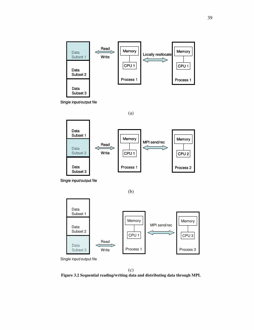
Figure 4.7 Performance of collective communication. (a) assigning the processes in

circular way; (b) assigning the processes in consecutive way. ....................... 52

Figure 5.1 The magnetic domain temporal evolution under vertical external magnetic

field. (a) time steps=0; (b)time=100; (c) time =500; (d) time =1000.............. 55

Figure 5.2 Magnetization curve simulated by parallel implementation and a simple

sequential program. ......................................................................................... 57

Figure 5.3 (a) Energy-minimizing domain configuration in growth twinned Terfenol-D

crystal. Magnetization vectors are aligned perpendicular to (111) growth

twin boundaries and form continuous 180° domains. (b) Schematics of

crystallographic orientations and magnetization easy axes (projected to the

plane of figure) of a pair of twin-related crystals (parent and twin). Only the

easy axes whose dot products with applied magnetic field Hex along c[112]

growth direction are non-negative are shown.43

.............................................. 59

Figure 5.4 Simulated magnetization curve in case (1) and (2).......................................... 61

Figure 5.5 Magnetic domain evolution for case (1). The vector plotted is the projection

of magnetization vector on the plane. The contour colors represent the

magnetization vector component out of the plane. ......................................... 62

Figure 5.6 Magnetic domain evolution for case (2). The vector plotted is the projection

of magnetization vector on the plane. The contour colors represent the

magnetization vector component in horizontal direction. ............................... 63

1

1 INTRODUCTION

1.1 Magnetic microstructure analysis

Magnetic phenomenon and magnetic materials, since their discovery, have been used for

a very long period of time. Lodestone, the material with a spontaneous magnetic state,

has been used in the compass to indicate north and south for almost two thousand years.

With today’s fast growing technology, magnetic materials find wider applications in

many fields. Among various magnetic materials, ferromagnetic materials, like iron,

nickel, cobalt, some of rare earths and their alloys, are widely used in permanent

magnets, information recording system, and so on. This is because ferromagnetic

materials exhibit many unique behaviors. For example, ferromagnetic materials can be

significantly magnetized under a relatively small applied magnetic field. Using this

property, electromagnets, such as iron core solenoids, can multiple an applied magnetic

field by thousand of times to generate large magnetic fields. After removal of the applied

magnetic field, ferromagnetic materials tend to keep their magnetized state, leading to

history dependent behavior, so called hysteresis. With this hysteretic characteristic,

ferromagnetic materials find important applications as information recording media.

Another important characteristic of ferromagnetic materials is magnetostriction, a

phenomenon of interdependence between magnetization and deformation.

This thesis follows the style of Applied Physics Letters.

2

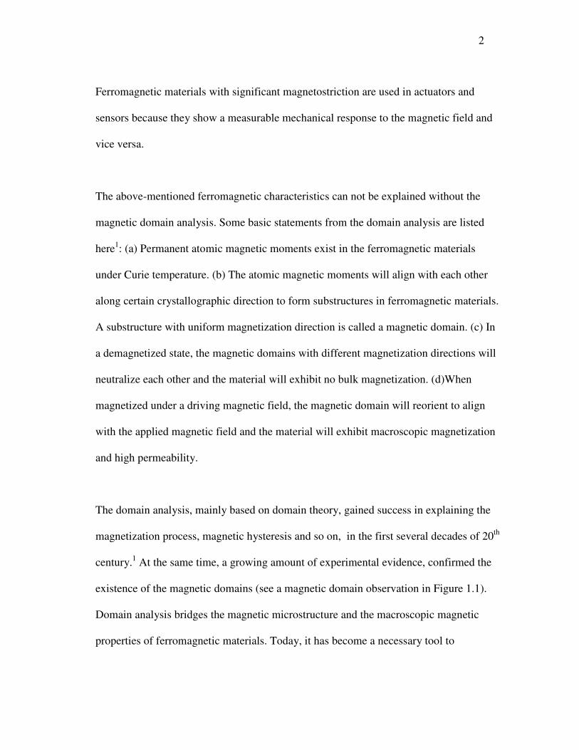
Ferromagnetic materials with significant magnetostriction are used in actuators and

sensors because they show a measurable mechanical response to the magnetic field and

vice versa.

The above-mentioned ferromagnetic characteristics can not be explained without the

magnetic domain analysis. Some basic statements from the domain analysis are listed

here1: (a) Permanent atomic magnetic moments exist in the ferromagnetic materials

under Curie temperature. (b) The atomic magnetic moments will align with each other

along certain crystallographic direction to form substructures in ferromagnetic materials.

A substructure with uniform magnetization direction is called a magnetic domain. (c) In

a demagnetized state, the magnetic domains with different magnetization directions will

neutralize each other and the material will exhibit no bulk magnetization. (d)When

magnetized under a driving magnetic field, the magnetic domain will reorient to align

with the applied magnetic field and the material will exhibit macroscopic magnetization

and high permeability.

The domain analysis, mainly based on domain theory, gained success in explaining the

magnetization process, magnetic hysteresis and so on, in the first several decades of 20th

century.1 At the same time, a growing amount of experimental evidence, confirmed the

existence of the magnetic domains (see a magnetic domain observation in Figure 1.1).

Domain analysis bridges the magnetic microstructure and the macroscopic magnetic

properties of ferromagnetic materials. Today, it has become a necessary tool to

3

understand macroscopic magnetic properties and to develop new magnetic materials. To

process the domain analysis, domain observation and micromagnetic theory are two

approaches that complement each other.2

Domain observation, such as Bitter patterns, magneto-optical methods, X-ray, and

transmission electron microscopy (TEM), can directly or indirectly reveal the magnetic

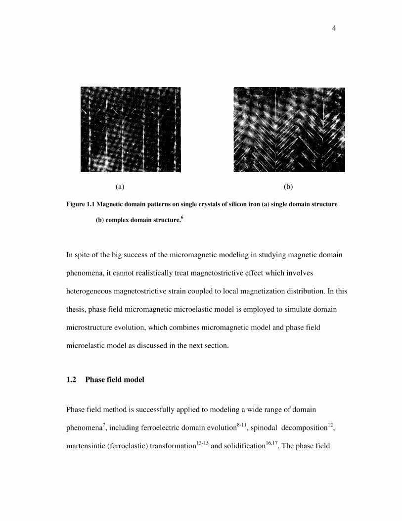
domain pattern based on different mechanisms. Figure 1.1 shows the domain pattern on

the surface of Si-Fe single crystal revealed by Bitter patterns.1 However, experimental

observations of domain evolutions under an applied field are time consuming and costly.

Moreover, the available observation technologies are limited to external surface while

the domain structure inside the bulk sample is not necessarily the same as that of

external surfaces. Given this limitation, the domain observation cannot offer enough

information to study magnetic domains in many cases.

Micromagnetism is an effective theoretical approach to studying domain structures. The

possible domain structures can be obtained based on the principle of total free energy

minimization.3 However, the micromagnetic equations are highly non-linear and non-

local. The minimization can be done analytically for very limited simple cases in which

a linearization is possible. Moreover, as mentioned previously, domain structures are

history dependent, so it is necessary to track the domain evolution in domain analysis.

Micromagnetic modeling, where the magnetization evolution equation is numerically

solved, offers a powerful simulation tool for domain analysis.4,5

4

(a) (b)

Figure 1.1 Magnetic domain patterns on single crystals of silicon iron (a) single domain structure

(b) complex domain structure.6

In spite of the big success of the micromagnetic modeling in studying magnetic domain

phenomena, it cannot realistically treat magnetostrictive effect which involves

heterogeneous magnetostrictive strain coupled to local magnetization distribution. In this

thesis, phase field micromagnetic microelastic model is employed to simulate domain

microstructure evolution, which combines micromagnetic model and phase field

microelastic model as discussed in the next section.

1.2 Phase field model

Phase field method is successfully applied to modeling a wide range of domain

phenomena7, including ferroelectric domain evolution

8-11, spinodal decomposition

12,

martensintic (ferroelastic) transformation13-15

and solidification16,17

. The phase field

5

method uses the spacial distribution of field variables to describe the domain

microstructures. For example, in decomposition the local concentration is used as the

field variable. Therefore, the domain with the homogenous physical property is

represented by the region with the homogenous field variables in the computational

region. At the domain boundaries, the field variables change continuously forming

smooth interfacial regions with finite thickness, i.e., diffused interfaces. For diffused

interfaces, there is no need to explicitly track the boundaries, which is a great advantage

of the phase field method.

The spacial and temporal evolution of field variables is described by the phase field

kinetic equations: Ginzburg-Landau equation for martensitic transformation18

, Cahn-

Hilliard equation for decomposition19

, and Landau-Lifshitz equation for magnetic

switching20

. The phase field variables obtained by solving the kinetic equations describe

domain microstructure evolution which decreases the system free energy and eventually

reaches the energy minimizing equilibrium state under given external condition.

Recently, a phase field micromagnetic microelastic model has been developed to study

the magnetic domain microstructure evolution in giant magnetostrictive materials, which

combines micromagnetic model of domain switching and phase field microelastic model

of martensitic transformation21,22

. The model is briefly described below.

6

The evolving magnetic domain structure in a magnetic material is described by

magnetization direction field ( )m r , whose average value gives the macroscopic

magnetization ( )sM m r (Ms being saturation magnetization). The total system free

energy for arbitrarily distributed magnetization field is a sum of magnetocrystalline

anisotropy energy Fani

, exchange energy Fexch

, magnetostatic self-energy Fmag

, external

magnetic energy Fex-mag

, elastic self-energy Fel, and external elastic energy F

ex-el:

1,21

F=Fani

+ Fex-mag

+ Fexch

+ Fmag

+ Fel + F

ex-el

= 2 2 2 2 2 2 2 2 2 3

1 1 2 2 3 3 1 2 1 2 3( )c c c c c c c c c

K m m m m m m K m m m d r + + + ∫ex 3

0 ( )s i iM m H d rµ− ∫ r

2 3( )A grad d r+∫ m r3

22

0 3

1( )

2 (2 )s

d kMµ

π+ ⋅∫ n m k

( ) ( ) ( ) ( )3

0 0 * ex 0 3

3

1

2 (2 )ijkl p ijpq qr klrs s ij kl ij ij

d kC n C C n d rε ε σ ε

π + − Ω − ∫∫ n k k r , (1)

where ( ) ( ) ( )c

i ij jm Q m=r r r , ( )Q r is rotation matrix field describing the grain structure,

1K and 2K are material constants characterizing magnetocrystalline anisotropy, A is

exchange stiffness constant, Hex

is external magnetic field, ~ indicates Fourier transform,

the integral ∫ is evaluated as a principal value excluding the point 0k = , kkn = , 0µ

is the vacuum permeability, ( )nijΩ is Green function tensor inverse to ( ) lkikjlij nnC=Ω− n1 ,

exσ is the external stress, and magnetostrictive strain field 0 ( )ε r is given as

0 ( ) ( ) ( ) ( ) ( ) ( (c

ij pqrs pi qj rk sl k lQ Q Q Q m mε α=r r r r r r) r) (2)

7

Under given external conditions, the evolution of magnetization field is described by the

Landau-Lifshitz-Gilbert equation:

( )( , )t t F Fγ δ δ α δ δ∂ ∂ = × − × ×m m r m m m m , (3)

where γ and α are the constants accounting for gyromagnetic process and

phenomenological damping.

The simulation of domain microstructure evolution in magnetic materials is performed

by numerically solving Eqs. (1)-(3) over discritized computational grids under given

initial and external boundary conditions. For such a computation, two major problems

arise; they are long computation time and large memory.

It is noted that, for a system of N computational grids, dipole-dipole interactions require

2( )O N number of floating point computation for each time step, which is reduced to

( log )O N N when a Fourier spectral method is adopted.17

For our simulations, it is

usually desirable to consider typical computation size of 512×512 and 256×256×256 for

2D and 3D simulations, respectively. Moreover, the number of time steps is usually as

high as one million or even more. Therefore, given current performance of a single

processor computer, the total computation time would be unacceptable, especially for

three dimensional problems.

8

Another serious problem for phase field simulations is the large memory requirement. It

requires a number of arrays to hold the field variables and related parameters associated

with all computational grids. For the typical simulation sizes used in phase field

modeling, the required memory size is far beyond the capability of a single processor

computer.

The phase field micromagnetic microelastic model described above allows all domain-

level mechanisms to operate freely, does not impose a priori constraint on the kinetic

pathways, accurately treats long-range interactions, and takes into account

magnetoelastic coupling due to magnetostriction. Therefore, the model is uniquely

capable for domain analysis to help reveal new domain mechanisms and develop new

magnetostrictive materials. However, its simulations demand for intensive computation

as discussed, and cannot be realized by a single processor computer available today.

Parallel computing offers an opportunity here.

1.3 Parallel computing

Parallel computation has been widely used in many fields for large scale scientific

simulations for decades, which effectively overcomes the limitations of sequential

computation operated by a single processor computer.23

The general strategy of parallel

computation is to make multiple computer resources work simultaneously on one

problem that does not fit on single processor computers. A large computational problem

is divided into smaller parts to be solved in parallel by multiple processors.

9

Based on the types of divided or parallelized units in a problem, the parallel computing

can be classified into four levels: Bit-level, instruction-level, data-level and task-level.

Most scientific parallel computation falls into the category of data parallelism handling

huge data but similar operation. “parallelizing loops often leads to similar (not

necessarily identical) operation sequences or functions being performed on elements of a

large data structure.”24

This is also true for the simulation of magnetic domains based on

the phase field model. In our simulation, the problem of formidable computer time and

memory requirement is solved by dividing the data associated with the whole simulated

volume into smaller subsets.

For parallel computing, the hardware architecture of the parallel computer is important.

Improper hardware architecture may not support the expected parallelism. There are

mainly two kinds of hardware architecture: shared memory multiprocessors and

distributed memory system. Their main characteristics are briefly explained in the

following.

In the shared memory architecture, multiple processors share the same memory, as

shown in Figure 1.2. Its advantages include fast memory access by all processors and no

need for communications among processors, and easy realization of parallelism for

computer programming. With certain programming interfaces, a programmer may easily

change the sequential code into shared memory multiprocessing program that

10

significantly reduces computer running time. However, shared memory multiprocessors

system can not scale well, and the number of multiprocessors involved in the parallel

computing is limited. It is also constrained by the available amount of the shared

memory.

Memory Hard disk

CPU CPU CPU CPU

Data bus

Memory Hard disk

CPU CPU CPU CPU

Data bus

Figure 1.2 The architecture of a shared memory multiprocessors system.

A distributed memory system has multiple independent memories and processors, where

a memory can only be directly accessed by the local processor. The architecture,

illustrated as Figure 1.3, allows much more memory and processors to be involved in the

parallel computation, compared to that of shared memories. Therefore, the problems

simultaneously requiring large memory and computation time can be solved through

parallelizing the program based on a distributed memory system. But this is not obtained

without cost. The complicated communications between processors arise. When a

processor needs data in the memory associated with another processor, it requires

communiation between the two processors through network, which costs significant

11

computer time. The true challenge we face here is the computer programming to

optimize communications among the processors.

Memory Hard disk

CPU

Memory Hard disk

CPU

Memory Hard disk

CPU

Memory Hard disk

CPU

Memory Hard disk

CPU

Memory Hard disk

CPU

Memory Hard disk

CPU

Memory Hard disk

CPU

Memory Hard disk

CPU

Memory Hard disk

CPU

Memory Hard disk

CPU

Memory Hard disk

CPU

Memory Hard disk

CPU

Memory Hard disk

CPU

Memory Hard disk

CPU

Memory Hard disk

CPU

Figure 1.3 The architecture of a distributed memory system.

For the simulations of domain structure evolution using the phase field model as given in

section 1.2, the parallel computing on a distributed memory system is a better choice.

Therefore, based on the distributed memory architecture, a more specified parallel

computing system, computer cluster, is selected as the computational platform. A

computer cluster is mainly composed of compute nodes and communication networks. A

compute node is similar to a traditional PC with independent processor and memory, and

12

the network requires high performance with low latency and fast bandwidth speed. The

technical details of the computer cluster will be introduced in next section.

1.4 Description of the thesis

This thesis begins with this Introduction. Development of a computer cluster system as

platform for parallel computation and the parallel algorithm for phase field model are

presented in Section 2 and Section 3, respectively. The performance evaluation of the

developed cluster system is introduced in Section 4. In Section 5, the parallel

implementation of phase field modeling of magnetization process in Terfenol-D crystals

is performed on the developed cluster system. The simulation results is presented and

discussed.

13

2 BUILDING CLUSTER SYSTEM FOR PARALLEL

COMPUTATION

2.1 Overview of a computer cluster system

A computer cluster is a high performance computing system consists of a group of

computers. The cluster, composed of multiple identical high performance computers

(compute nodes) and high performance network, is an ideal platform for scientific

parallel computation. Figure 2.1 shows the topology of a general computer cluster. By

integrating multiple linked compute nodes into a single cluster under uniform

administration, the system performs as a single supercomputer. Computer clusters retain

a reasonable price without compromising computation power. Due to these advantages,

the computer cluster has become the mainstream of high performance computation and

widely used in the field of science, engineering and business. From the TOP500 list of

World’s Most Powerful Supercomputers of year 200825

, 80% of supercomputers are

computer clusters.

Clusters are divided into two types: custom cluster and commodity cluster. By

customizing the compute nodes, networks and operating system, the custom cluster can

obtain excellent performance to support parallel computation but at a very high price. In

contrast, commodity clusters are mainly composed of commercial off-the-shelf hardware

and open source software so that cost can be minimized while performance can be

14

maximized. Considering the requirement for the computational performance and a

limited funding, commodity cluster would be a reasonable high performance

computation solution for small research groups. A book26

for guiding how to build a

commodity cluster was provided by Sterling et al. as a good handbook for developing a

such cluster system

The cluster system mainly consists of compute nodes and networks. Besides being

compatible with the given hardware, the software system must meet the needs of

administration and management, and support parallel computation. Like developing any

other computer system, selecting and deploying hardware system as well as building the

software environment are the main tasks when constructing a cluster system.

Master

Compute

node

Network switch

Slave

Compute

node

Slave

Compute

node

Slave

Compute

node

Master

Compute

node

Network switch

Slave

Compute

node

Slave

Compute

node

Slave

Compute

node

Figure 2.1 Topology of computer cluster.

15

2.2 Hardware system structure

2.2.1 Compute nodes

The configuration of each individual compute node is one of the most important

considerations in the development of a computer cluster. Generally, each individual

compute node is an independent computer. The procedure of configuring each individual

compute node is similar to the procedure for configuring a conventional PC. Four basic

components, the processor, main memory, motherboard, and hard disk, are to be

considered and will determine the general performance of the nodes. The space occupied

by the compute node must also be considered when many compute nodes are

incorporated into the cluster. The commodity cluster may utilize either rack-mounted

servers or PCs as its compute nodes. Although the price is higher, the rack-mounted

server has a more powerful computational ability. Also, the uniform compact structure

of the rack-mounted serve make it easily attachable to the standard enclosure for good

organization and great space saving.

There are two kinds of nodes in the cluster though they both are called compute nodes:

Master nodes, and slave nodes. Master node will control other nodes to form a uniform

system so that the group of nodes would act as a single computer. For small cluster with

a limited number of nodes, a single master node would be sufficient for the control and

management work of the whole system. Conversely, slave nodes are controlled by a

master node to work on assigned job. The master node usually has better performance,

16

such as larger storing capability and faster processors, to support the management of the

whole system. It may or may not directly take part in the parallel computation jobs based

on the situation of load balance. For slave nodes, identical configuration is suggested to

simplify the cluster system and maintain the load balance for parallel computation.

The number of nodes is another important factor to determine the computation capability

of the whole system. More compute nodes included in cluster would involve more

processors in the system and naturally increase the computation capability. For example,

1100 Apple Xserve G5 system serve as compute nodes in the System X cluster at Virgin

Tech27

, which delivers an incredible computation speed of 12.35 TFlops, was the fastest

supercomputer in 2006 all over the world according to the TOP500 list of World’s Most

Powerful Supercomputers. However, the float operation per seconds can not fully

describe the performance of users’ practical parallel application on the cluster. Actually,

many parallel implementations may run satisfactorily on a computer cluster with no

more than 32 processors, due to the scalability of the program and other factors.

Therefore, the number of compute nodes must be carefully considered according to the

requirement of potential parallel computation.

2.2.2 Communication network

A communication network system connects the compute nodes to form an integrated

cluster system. In parallel computation, it is used to transfer data among different

compute nodes. The hardware of a general network system includes a switch, an

17

interface on the compute nodes and cable. Like compute nodes, hardware for the

network is also based on commercial commodity. For example, common and economical

Ethernet-based networks are most frequently utilized in clusters. But a better

performance network with a much higher price is necessary for some parallel

computation that involved intense data communication. Therefore, the choice of network

hardware is highly dependent on the requirement of potential parallel computation.

In parallel computation, the network is used to deliver information or data among

compute nodes. Its performance is described mainly by its bandwidth and latency.

Bandwidth is the average rate of information or data delivered via the network. It is

usually measured by Bit/s. Higher bandwidth speed will significantly decrease the

delivery time, especially for the information with large size. The latency is related to the

delay of the information delivered, which is mainly caused by the required responding

time between compute nodes to send and receive information. The efficiency of

delivering information or data with small size is very sensitive to the latency because the

delay time, rather than the direct transferring time, takes the main part in the whole

delivering time.

There may be one or two network systems in one computer cluster. The first

management network is usually an IP-based Ethernet private network. This network is

used for sending and receiving controlling messages. Through this network, master node

can reach the whole cluster system by sending instruction to slave nodes, maintain the

18

operating system, and manage the parallel jobs and so on. Because the management

messages delivered are usually relatively small, an Ethernet-based network with

moderate performance can satisfy the management requirement. If the computer cluster

is used to run some parallel implementation without intense data communication, this

management network may also be used to support the data communication among

compute nodes in parallel computation. In that case, a single high performance Ethernet-

based network will support all communication and no secondary network is needed.

Some parallel application involves intensive interprocess communication to share the

data among different nodes. In that case, it is recommended to separate interprocess

communication from the management messages through building a secondary high

performance network. The computer time consumed by a parallel program consists of

two parts: the direct computation time and interprocess communication time. A high

performance network with wide bandwidth and low latency would significantly decrease

the communication time. Through that, a decreased total computer time and better

scalability may be obtained for parallel programs. Due to the critical role played by the

network in intensive communication parallel computation, some advanced network

technology such as Infinitband and Myrinet, at much higher price, will be used in this

secondary high performance network instead of ordinary Ethernet-based system. And if

the secondary network is applied, the first management network is only required to have

moderate performance to save money.

19

2.2.3 Other hardware components

Some support components are also necessary for the cluster system. If compacted rack-

mounted servers are chosen as compute nodes, a cooling system is critical to prevent

system failure by over-heating. It will remove the system heat output, which mostly

comes from the compacted rack-mounted servers. Also, a backup power supply is

needed to prevent damage due to a power surge. Finally, all of this hardware needs a

standard enclosure for storage.

2.3 Software environment for cluster system

2.3.1 Operating system

An operating system of computer cluster works both for the compute node itself, just

like an ordinary PC, and also for the whole network system of the cluster. A

sophisticated operating system for a cluster is used to manage each node such as

configuring all of hardware resources, managing user accounts, managing memory,

hosting application program, and so on. Also, the cluster operating system is in charge of

administration and management of the whole cluster system, creating a uniform software

environment, building the distributed file system, configuring the private communication

networks, and so on.

20

2.3.2 Communication mechanism and implementation

Complex parallel computation requires intense communication for sharing data,

synchronizing processes and so on. This communication can be done by “message

passing” for distributed memory system or multithread for SMP (share memory

multiprocessors). In the distributed memory system, like cluster, through “sending” and

“receiving” messages containing needed data or other information, the compute nodes

involved in parallel computation can communicate with each other. Therefore, a

standard of message-passing become necessary to formalize the communication style. A

corresponding software implementation will work with programming language, through

that programmers can control the interprocess communication in their programs.

It is noteworthy that this communication mechanism is highly dependent on the

architecture of hardware. As mentioned above, “message passing” communication is

mainly based on a distributed memory system, but contemporary clusters usually utilize

SMP computers as compute nodes. In another word, the whole cluster is a hybrid system;

inside of each node, it has the architecture of share memory multiprocessors while

among the compute nodes it is a distributed memory system. This complex structure,

called a distributed SMP system, makes the interprocess communication more difficult

than pure distributed memory system or SMP system. Generally, a mixture of message

passing and multithread communication mechanisms would optimize performance in a

hybrid system; however, this would greatly complicate the programming. How to build

an optimized communication mechanism on this hybrid SMP cluster system is still under

21

research. Today, a message-passing communication is typically used exclusively in a

SMP nodes cluster though it is obviously not the best choice.

2.3.3 Workload management software

The workload management software is used to manage computing resource for the user

applications. Usually, there are multiple users served by a cluster system. A usage policy

sets the priority to use computing resource for the applications submitted by different

users. For example, some users may always have the highest priority to use the

computing resource, or, only the parallel application submitted by certain group of users

may use more memory or computing nodes. The workload management software will

combine the current state of the cluster system and carry out such sets of policy to

manage the usage of computing resources. Generally, there are five responsibilities for

the workload management software:

1. Queuing

When users want to run any task on a cluster, a job must be submitted to the workload

management system with enough information about this task, like user’s account, the

needed number of CPU, the amount of memory, the file to execute, and the path storing

output files. With the information of submitted jobs, the management system will follow

the usage policy to rank all of submitted jobs to form a job queue. The jobs will be

executed following the sequence of the queue whenever the needed computing resources

become available. Through this queuing system, different usage policies can be carried

out. The administrator can designate top priority to certain users in order to prevent them

from waiting in queue. Also, it may prefer to run small tasks during daytime to serve

22

more users, but to run tasks which consume substantial computing resources and

computer time at night. These kinds of restrictions can be realized by the queuing

function of workload management software on the cluster.

2. Scheduling

Usually, the usage policy given by the administrator can not fully define the executed

sequence of submitted jobs. A scheduler will also be used to choose the best job to run.

The scheduler will consider the usage policy and current available computing resources

to run the best job and optimize the usage of computing resources.

3. Monitoring

The monitoring in workload management software will provide information about

computing resources. It will check the state of the compute nodes before assigning jobs

in order to assure the compute nodes are error free and meet the requirement of assigned

jobs; any discrepancies be reported to system.

Another important application of resource monitoring is to report the performance of

running jobs. All of important information such as the usage of CPU, memory, network

and other resources on a certain job can be viewed through the monitoring function.

With this information, users can evaluate and improve their parallel program. For

example, if the resource monitor reported more than 90% computer time was consumed

by communication, then the data communication strategy within the program need

requires substantial improvement.

23

4. Resource management

Once a job is submitted to the cluster system and determined as the current best job to

run, the workload management software will automatically run the job on the

corresponding computing resource, and when the job finishes, it will stop the application

and clean up for the next job. These processes are called resource management.

5. Accounting

This function will collect the information of resource usage for certain jobs, users, and

groups.

2.3.4 Other software

Some support software would also be necessary when running the aforementioned

software. For example, the message passing communication would require OpenSSH as

the tool for remote logging from master node to slave nodes.

Also, additional commercial software may be required according to the specific

application of users. Some commercial software companies already offer the edition

applied for cluster and parallel computation; MATLAB introduced a distributed

computing toolbox to support parallel computation on clusters. GridMathematica also

delivers a parallelized Mathmatica environment for cluster platform. Such commercial

software will allow user to simply explore the advantage of cluster as a parallel

computation platform without messing up with complex parallel algorithm.

24

2.4 Deploying an 8-nodes Apple workgroup cluster with high performance

networks

Our Apple workgroup cluster selects 8 powerful Xserve/Intel servers as compute nodes.

Mac OS X server, the UNIX based operating system is preinstalled on these servers.

Xserve/Intel server integrates and optimizes all of hardware needed for computing nodes,

such as processors, memories and network interface to deliver powerful computation

capability. The Mac OS X server operating system is customized by the same vendor of

servers to optimize the performance of single node. This operating system already

includes many tools for administration and management of the whole distributed

memory system.

2.4.1 Compute nodes

Two 2.66 GHz Dual-core Intel Xeon processors have been selected for every SMP

compute node mainly due to two considerations: the first is that this processor one

generation behind the cutting edge, usually has best performance/price. Another reason

is that previous computation on other clusters has shown that satisfactory speed can be

obtained only if the processors have clock rate above 2.0 GHz. Although faster

processors are always welcomed by users, overall performance/price is the key for

configuring a system. Especially for a platform of intense parallel computation, the

performance of networks, not the processors, are usually the bottleneck of computation,

so the newest and fastest processors costing much funding are most likely not to greatly

improve the overall performance.

25

The capability of main memory is very important for scientific and engineering

simulation. The problem of “out of memory” is fatal, and prevents researchers exploring

some problems interesting but too large (e.g. some 3-dimensional simulation). Therefore,

a memory requirement for possible largest simulation for phase field model of magnetic

domain has been estimated. It shows that the amount of memory, for every compute note

with two Dual-core processors, should be about 8 gigabyte. Accordingly, the total

memory would be 64 gigabyte.

The capability of hard disk is 80 GB for compute nodes according to the principle that

local disk capacity should be ten times the main memory capacity. But a much larger

hard disk (750 GB) is selected for master node for the management work and temporally

storing users’ data files.

2.4.2 Interconnect networks

The first management network for the cluster is an Ethernet private network mainly

based on 3com 24-port baseline switch, which is a highly affordable, unmanaged Gigabit

switch. This gigabit switch has 100MBps bandwidth and around 210 us latency.

Myrinet is selected as the second interprocess network system for the Apple workgroup

cluster. Myrinet, designed by Myricom, is one of the best network solutions for parallel

computation with intensive communication. Myrinet has fast bandwidth and low latency.

According to Myricom, the latency of this Myrinet-2000 switch network for data

communication using Message Passing Interface (MPI), an implementation of parallel

26

communication, is only 2.6µs–3.2µs, and the MPI unidirectional data rate is 247

MBytes/s. An advantage of Myrinet is that this Myrinet-2000 switch has independent

processor and memory so that the data transmission would not take the main processor

clock time to interrupt the process. This feature will significantly improve the efficiency

of parallel computation.

To build Myrinet high performance network, a 16-port Myrinet-2000 switch and 8 PCI-

X NICs as network interface cards have been selected for the 8-node Apple cluster. The

switch has 8 ports available for potential update adding more computing nodes into the

system.

2.4.3 Other hardware components

According to Apple Company, the thermal output per Xserve/Intel server is about 1100

BTU/h. So a cooling system with capacity removing at least heat output of 11000 BTU/h

is required with 20% headroom for eight compute nodes. But considering the potential

of adding more compute nodes, a rack air removal unit with much higher cooling power

has been equipped.

APC 1000VA Uninterruptibel Power Supply (UPS) has been selected for protecting

head node and networks from damage due to power surges.

27

NetShelter enclosure, a standard enclosure for storage of 19-inch rack –mount hardware,

is selected to accommodate all of hardware including eight compute nodes, two sets of

networks switches, rack air removal unit, UPS, and so on.

Appendix A. gives the information of hardware to deploy an 8-node Apple workgroup

cluster with high performance network. Figure 2.2 shows the eight Apple Xserver

computing nodes, and figure 2.3 shows the completed cluster system.

Figure 2.2 Eight Apple Xserver computing nodes.

28

Figure 2.3 Apple workgroup cluster system.

2.4.4 Mac OS X Serve operating system

The Mac OS X Serve, designed by Apple Corp for Xserve server, is a powerful

operating system for administration and management of workgroup cluster. Its

convenient and nice-interface management tools make administration of computing

resources and users accounts much easier than traditional Unix/Linux system. At the

same time, this UNIX based operating system inherits the main advantages of

Unix/Linux system, like supporting almost all of open source software for UNIX/Linux

system. In fact, Mac OS X already integrates more than 100 open source projects

including OpenSSH, X11, GCC, and so on most used tools.

29

In addition to the basic administration and management function, Mac OS X Serve also

has many advantages for scientific computation. It fully supports 64-Bit computing. The

64-bit addressing of the operating system provides the capability of accessing large

memory, and what is more excited for high-performance computation, Mac OS X Serve

already includes many 64-bit optimized math libraries for the hardware of Xserve

servers, such as BLAS, LAPACK, vBigNum (a vector big number library), vBasicOps

(a basic algebraic operations library). All of these math libraries can be easily call from

C or Fortran program.

2.4.5 MPICH2 for message passing interface in parallel computation

As 2.3.2 mentioned, a message-passing communication mechanism is used globally in a

SMP nodes cluster. The message passing process is specified by Message Passing

Interface (MPI)28

. MPI provides a set of standards for message passing communication,

and these standards now have been developed as so-called MPI-2. MPICH229

, developed

by Argonne National Lab, is chosen as the implementation of MPI-2. The actually used

in the cluster is MPICH2-MX30

, which is a port of MPICH2 on top of MX (a low-level

message-passing system for Myrinet networks) developed by Myricom to optimize

Myrinet networks performance for MPI application.

30

3 PARALLEL COMPUTATION FOR PHASE FIELD MODEL

3.1 Domain decomposition

As 1.2 introduces, the magnetic domain structure is described by the spatial distribution

of local unit magnetization vector ( )m r . Its evolution is then reflected by the evolution

of ( )m r , which is obtained at every computing grid by solving equations (1)-(3). A

number of huge data associated with the computing grids are used to accommodate the

intermediate results, the updated unit magnetization vector field, and other information

such as free energy density for each cell. How to handle these huge arrays storing the

information associated with each grid is the key for the parallel computation applied here.

As 1.3 introduced, the parallelism in our simulation is mainly based on the data-level

parallel model. In this model, the computational domain of a problem is distributed

among compute nodes. Each compute node has certain subset of the data stored on its

local memory, and the processor will perform task mainly based on its local data. Figure

3.1 illustrates this method. The computational domain is divided into four subsets with

equal size. The data associated with the grid are distributed across four different

compute nodes. The processor of each node will perform very similar operation but only

on the subset stored on local memory. Through this so-called domain decomposition

operation, the huge data array storing large computational domain is easily

accommodated by multiple memories on involved compute nodes. This is the very

31

reason that the data-level parallel computation on distributed memory system can handle

the problem of inefficient memory on traditional PC.

In the domain decomposition shown as Figure 3.1, the divided subsets have identical

size and geometry. But equally decomposing domain is not the universal solution. The

domain decomposition must follow several general rules.

The domain decomposition is directly related with the work load assigned to each

compute node. And the load balance is the critical for the efficiency of parallel program.

Poor load balance among different compute nodes will seriously break down the

program and waste compute resource. The whole parallel program completes only when

all of compute nodes complete their subtasks. During this period, the compute nodes

cannot be released for new task even if some compute nodes may be idle after

completing their own subtasks. The ideal case is that all of compute nodes complete their

subtasks at same time. To do so, balance load control is necessary. If the compute nodes

have very similar operation on the subsets of data, the operation time is mainly

dependent on the size of data. Therefore, the computational domain is naturally

decomposed equally, which is just the case of our simulation. But in some complicated

situation, the subtasks scale may differ. In those cases, there is no general method to do

the domain decomposition. Some advanced method, like monitoring the load balance

and real-time adjusting it, may be needed to maintain the parallel performance.

32

Another important reason to equally decompose computational domain is due to the

similar calculation operated by compute nodes. On each node, the equation is solved

following almost the same procedures though the data are different. It would be easy for

programming loops when the subsets of computational domain have identical size and

shape.

1 64 128

64

128

1

Subset 3 Subset 4

Subset 1 Subset 2

(a)

Subset 3Subset 1 Subset 2 Subset 4

Node 1

CPU 1

Memory 1

Node 2

CPU 2

Memory 2

Node 3

CPU 3

Memory 3

Node 4

CPU 4

Memory 4

network

Subset 3Subset 1 Subset 2 Subset 4

Node 1

CPU 1

Memory 1

Node 2

CPU 2

Memory 2

Node 3

CPU 3

Memory 3

Node 4

CPU 4

Memory 4

network

(b)

Figure 3.1 Domain decomposition (a) original computational domain with 128*128 grids. (b) Four

subsets of the original computational domain are distributed across four compute nodes.

33

To decrease data communication among compute nodes is another important

consideration when decompose domain. Comparing with traditional sequential

programming, complex data communication among compute nodes is the disadvantage

for parallel computing based on distributed memory system. The overhead from data

communication may greatly increase the computer time, which seriously worsens the

performance of parallel computing. Therefore, the domain should be decomposed in a

way that the data communication is as little as possible and most of calculation can be

supported by local data.

3.2 Data communication based on MPI

Data communication is important in the parallel programming especially on the share

memory system. A good data communication control means low overhead and most

CPU time is attributed to the data computation rather than communication. MPI

(Message Passing Interface) is used in our parallel programming as the communication

standard, and MPICH2 is the corresponding implementation applied. The main features

of MPI and some important MPI routines are introduced here, followed by the data

communication strategy in our program.

3.2.1 Message passing interface

MPI is a communication protocol in parallel computation mainly for distributed memory

system while it still can be used for share memory computer. The goal of MPI is “to

develop a widely used standard for writing message-passing programs”. It provides the

34

standards of the process topology, synchronization, point-to-point communication,

collective operations, and other operations involving in communication of parallel

computation. In MPI, the communicated data is packaged in a message and passed

among multiple processors. MPICH2, used by our cluster, is a high-performance

implementation of MPI standard. It has a specific set of routines which can be called

from Fortran or C language. The implementation of MPI allows programmer manage the

data communication by programming.

Unlike the sequential computation, parallel computation based on MPI involves many

operations directly controlling the processors and network. We need to understand the

architecture of actual used cluster before using MPI control the communication.

Globally, there are eight compute nodes connected by network to form the distributed

memory system. But for each node, it is a shared memory computer with two CPUs. In

each CPU, there are two cores which can perform the instructions independently. A

processor or process defined in MPI should be taken as a single core in our cluster. In

another word, the Apple 8-node cluster has 32 processors for parallel computation.

Based on the knowledge of the architecture of our cluster, we can introduce how MPI

works in the data communication.

Firstly, every MPI session needs a communicator to include a group of processes. Here,

the process, originally means the set of sequentially executed instructions, always can be

taken as the processor. For example, four cores in two dual-core CPU would be included

35

in a communicator if users require four processes in the parallel computation. There may

be more than one communicator in one session to control several groups of processors.

In each group, the processors are identified by a unique integer between zero and the

number of processors. In our parallel program, only one communicator is used.

Once the communicator is set up, the processors can be identified so that the message

can be passed among specific processors. There are two types of data communication

applied in our program. The Point-to-Point communication will pass data between two

specific processes while collective communication happens among all of processes in the

group. The Point-to-Point communication has blocking and non-blocking mechanisms.

The blocking communication has some extra operations to assure the process receiving

message is ready and waiting for the message. It gains more security but with slower

speed compared with non-blocking communication. Both mechanisms have application

in our program.

MPICH2 offers routines to manage the data communication operations, like initializing

and terminating the MPI process, passing and collecting data among processors. Some

important routines used in our fortran program are introduced as follows.

MPI_INIT(ierr)

This routine initializes the MPI execution environment to start a MPI process.

MPI_COMM_SIZE(comm.,size,ierr)

This routine determines the number of processes involved in the group.

36

MPI_COMM_RANK(comm.,rank,ierr)

This routine determines the rank of the calling process. The parameter “rank” will return

a unique integer between 0 to the number of process in the group, which will be used to

identify the processor.

MPI_Bcast (buffer,count,datatype,root,coom,ierr)

This routine broadcast a message from one certain process to all other processes

involved in the communication group. The message or data address is specified by the

parameter buffer, and the process sent message is identified by the parameter root, which

is its rank in the group. The parameter count specifies the message size.

MPI_Send (buffer,count,datatype,dest,tag,comm.,ierr) `

This routine sends data located in “buffer” to the process with rank as “dest”. This

operation is labeled by the parameter tag.

MPI_Recv(buffer,count,datatype,source,tag,comm.,status,ierr)

This routine receive data sent from process with rank as “source”. The received message

is labeled by the parameter tag. This routine always works with MPI_Send to complete

the message passing.

MPI_Barrier(comm.,ierr)

This routine makes synchronization in a communication group. Every process will block

at the MPI_Barrier routine until all processes in the communication group reach same

MPI_Allreduce(sendbuffer,recvbuffer,count,datatype,op,comm.,ierr)

This routine operates a reduction and writes the results in all process.

37

From the above description, it shows that the data communication control in the

programming is realized by simply setting parameters and calling proper MPI functions.

Through that, MPI and its implementation MPICH2 offer a convenient way to directly

control hardware such as the processors and network to realize the data communication

among independent compute nodes.

3.2.2 Data read and write in parallel computing

Equation (3) is an initial value problem for each grid, so the initial information, like the

initial unit magnetization vector on each computing grid must be given to start the Euler

scheme. Therefore, program needs to read a huge input file with initial information to

start the iteration. In addition, these data associated with the mesh of computing grid

must be assigned to different computing nodes as Figure 3.1 shows. The first problem in

parallelizing the iteration is how to read the initial data from input files and assigned the

data to multiple computing nodes. Accordingly, an opposite problem is how to collect

the resulting data from computing nodes and output them to several files in right

sequence after the iteration is finished. This parallel reading and writing problem will be

discussed here.

It would be ideal if each computing node can directly read from (or write to) the same

file simultaneously. Unfortunately, parallel I/O may induce some serious problem; the

output file may be overwrote by the multiple writing operation, the parallel reading may

not be supported by ability of the operating system to handle multiple reading operation

38

at the same time. At current technology a parallel I/O system is still uncertain, some

compromise must be made to perform the parallel reading and writing operation.

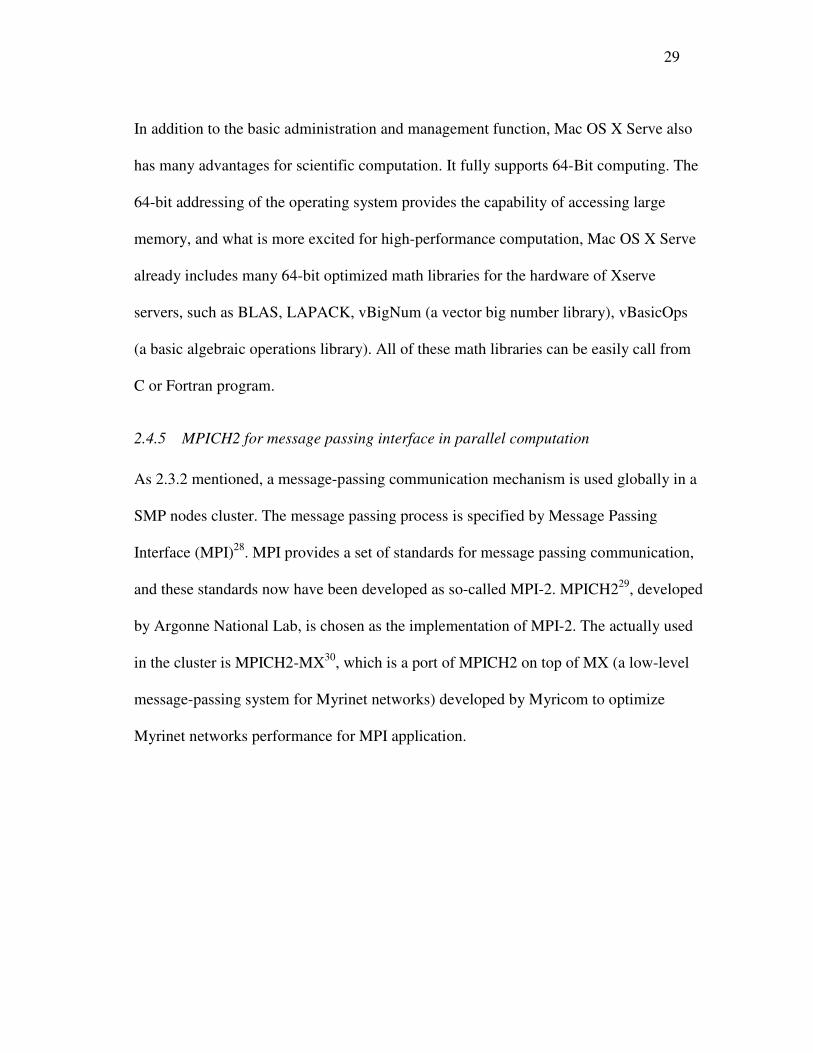
In our program, sequential rather than parallel reading and writing is applied. There is a

process, say the one with rank 1, will handle main operation. The operation includes

reading from (or writing to) a single file, distributing input data or collecting resulting

data among the local memories of multiple processors in the communication group, and

reformatting those data. The actual reading procedure for a parallel implementation is

shown as Figure 3.2.

Three processes are assumed to take part in the parallel computation without loss of

generality. The process 1 firstly reads the first part of input data and locates them in its

local memory. It continues to read the second part of data and uses the MPI routine

MPI_Send to send this part of data to process 2. The similar operation follows the

second step except that the destination of third part of data is process 3. Accordingly, the

process 2 and process 3 will call routine MPI_Recv to receive the data sent from

process1 and locate them on their local memory. The opposite operation, writing

resulting data to single file, can be figured out in similar way.

It should be pointed out that the MPI sending or receiving operation during above

procedure does not have to happen among multiple compute nodes via network. As 2.1

mentioned, the cluster used here is a hybrid system with shared memory computer as

39

Data

Subset 3

Data

Subset 1

Data

Subset 2

Read

Write

Single input/output file

Locally reallocateMemory

CPU 1

Process 1

Memory

CPU 1

Process 1

Data

Subset 3

Data

Subset 1

Data

Subset 2

Read

Write

Single input/output file

Locally reallocateMemory

CPU 1

Process 1

Memory

CPU 1

Process 1

(a)

Data

Subset 3

Data

Subset 1

Data

Subset 2

Read

Write

Single input/output file

MPI send/recMemory

CPU 1

Process 1

Memory

CPU 2

Process 2Data

Subset 3

Data

Subset 1

Data

Subset 2

Read

Write

Single input/output file

MPI send/recMemory

CPU 1

Process 1

Memory

CPU 2

Process 2

(b)

Data

Subset 3

Data

Subset 1

Data

Subset 2

Read

Write

Single input/output file

MPI send/recMemory

CPU 1

Process 1

Memory

CPU 3

Process 3

(c)

Figure 3.2 Sequential reading/writing data and distributing data through MPI.

40

compute node. Therefore, the multiple processors involved in the communication group

may belong to the same compute node. As we know, the data communication inside

single compute node is much faster than that among multiple compute nodes. It is very

important to understand this character to optimize the performance of the parallel

implementation on the cluster with hybrid structure.

A similar consideration in above example exists when the first process reads the input

data file on the hard drive. Through open directory file system, the common directory

accommodates the I/O files and physically locates on the hard drive of the head node in

our cluster. Other compute nodes can access the common directory via network, but the

access speed is much slower than that accessing local hard drive via data bus. Therefore,

if the first process in charge of reading file from hard drive can be assigned to the head

node, it will read input file directly from local hard drive through data bus. Especially for

the situation involving frequent I/O operation, like intense backup of huge intermediate

results, this kind of optimization should be considered.

The sequential reading and writing operation and distributing data through MPI can

handle files with moderate size, which is just the case of our current simulation. If the

simulation size goes much larger in future, some complex parallel reading and writing

technology have to be introduced in our programming. A book by John M. introduces

some advanced methods to realize parallel I/O31

.

41

3.3 Parallel fast Fourier transformation

After the initial data is read and distributed, the iteration based on Euler scheme can start

simultaneously on multiple processors in the group. At each step, the main task is to

calculate the driving force, Fδ δm , based on current unit magnetization vector field.

But the calculation of driving force for each grid is highly dependent on the information

related with all other grids in the computational region.

With periodic boundary conditions, fast Fourier transform (FFT) method is often

employed to deal with the non-local computation when solving phase field equation32,33

.

The method “converts the integral-differential equations into algebraic equations”7. The

complexity for the direct computation of interaction between magnetization

vectors, 2( )O N , will be reduced to ( log )O N N by using fast Fourier transform.

If FFT is implemented in our parallel program, the algorithm of FFT must be

parallelized compatible with the parallel program. Because of the wide use of FFT, many

references can be found on parallelizing FFT method. However, few parallel FFT codes

are publicly available. 2D and 3D parallel FFT subroutines are developed by our group.

42

4 THE PERFORMANCE EVALUATION OF APPLE

WORKGROUP CLUSTER

The performance evaluation includes two parts: test of the software environment to see if

the cluster supports general MPI program, and test of data communication performance

on the workgroup cluster.

4.1 Verify MPI functions

The developed Apple workgroup cluster is to serve as parallel computing platform for

MPI programs. After the software environment is set up, all MPI functions must be

carefully tested. The error checking will assure the cluster system can perform as a

capable platform of MPI programs.

Some initial tests can be done by directly running the example programs, which come

with MPICH2 software. If these programs successfully run on the cluster and return

correct results, then a more thorough test is run with the command “make testing” from

the top-level of mpich2 directory. It produces a summary of the test results. From the

summary, all function related with the MPI functions in fortran program are error free in

our cluster system.

43

4.2 Data communication performance

4.2.1 Benchmarking point-to-point communication

The MPI functions test only can determine if the installed version of MPICH2 is

functioning in the current cluster system. But users may be more interested in the

performance of their parallel implementation on the cluster system. Besides of the

parallel implementation itself, the data communication performance is the most

important factor to determine the overall performance of the potential MPI program.

Given some performance parameters on the data communication, users may be able to

estimate the performance of their MPI programs on the cluster system.

The program mpptest is a performance test suite. This program is distributed with

MPICH2. Once the MPICH2 is installed successfully, the executable, mpptest, is already

available. It measures the MPI-based communication performance in several ways to

reflect the performance.

By measure some important parameters during the communication, mpptest provides a

clear picture both for point-to-point and collective communication performance on our

cluster system. In our implementation, block and non-blocking point-to-point

communication, and collective communication are operated. Therefore, the mpptest is

conducted based on these three types of data communication.

44

Figure 4.1 and Figure 4.2 show the performance of a single message sent between two

processes based on blocking and non-blocking communication, respectively. The

bandwidth and latency, two important parameters in communication, are revealed by the

tests. The size of messages is automatically chosen in order to reveal the message size

where the change of behavior happens.

From Figure 4.1 and Figure 4.2, the latency for small massage is about 4 microseconds,

and the maximum bandwidth is about 220MB/sec. The same parameters based on

similar hardware, reported by Myrinet, are used to compare with our performance

parameters. According to the report from Myrinet, the maximum bandwidth is about 230

MB/sec, and the latency for empty message is about 9 microseconds, which proves that

our cluster system have obtained the expected performance in point-to-point

communication.

The point-to-point communication tests provide us with certain confidence that the

cluster system is functioning properly. Also, the test results show the best bandwidth

performance dependent on the message size. From Figure 4.1(b) and Figure 4.2(b), a

sudden drop in bandwidth happens when message size is increased to about 32000 bytes.

This information may be useful when users try to control the message size to optimize

their implementation performance.

45

(a) (b)

(c) (d)

Figure 4.1 Performance of blocking communication based on MPI_send routine.(a)latency for short

message (b) bandwidth for short message (c) latency for long message (d) bandwidth for

long message.

46

(a) (b)

(c) (d)

Figure 4.2 Performance of non-blocking communication based on MPI_send routine(a) latency for

short message (b) bandwidth for short message (c) latency for long message (d)

bandwidth for long message.

Another interesting phenomenon, revealed by the point-to-point communication test, is

shown as Figure 4.3.The previous point-to-point communication tests are all conducted

between two compute nodes via Myrinet network. However, the developed Apple

workgroup cluster is based on shared memory computer nodes. The point-to-point

communication can also be operated between two processors within the same compute

node. In that situation, the data bus, rather than the Myrinet network, will be in charge of

47

the communication, and support faster communication speed as Figure 4.3 shows. This

communication performance difference may affect the way we distribute parallel tasks

among our cluster system.

Figure 4.3 Point-to-point communication latency in distributed memory system and shared memory

system.

4.2.2 Benchmarking collective communication

Another important data communication type applied in our parallel implementation is

collective communication. Mpptest also can measure the communication performance

based on this data communication type. The measured communication performance of

MPI collective communication routine, MPI_reduce, is showed as Figure 4.4, which

48

behaves similarly with the one according to the report of Myrinet Company. Like point-

to-point communication, a sudden behavior change happens where the message size is

increased to 1000 bytes.

(a) (b)

Figure 4.4 Performance of collective communication based on MPI _reduce routine.

(a)latency; (b) bandwidth.

Unlike point-to-point communication, collective communication involves multiple

processes. As the number of involved processors increases, some MPI routines may

induce a latency cost proportional to the number of processors. Therefore, scalability is

another important consideration to evaluate a collective communication on our cluster

system. Goptest, a MPI benchmarking program distributed with MPICH2, is used to test

this property. Goptest will measure the collective communication performance

dependent on the number of processors.

49

Figure 4.5 shows the average time for collective communication dependent on the

number of processors. The tested MPI routine is MPI_reduce, and the message size

varies from 256 bytes to 1024 bytes. From Figure 4.5, the message passing time does not

increase significantly as the number of processors increases. This trend implies that the

collective communication will not break down as more processors join in the group.

Figure 4.5 Performance of collective communication dependent on number of processors.

An interesting phenomenon related with the hybrid architecture of the Apple workgroup

cluster is found in goptest. Before introducing it, a related background about how

MPICH2 assigns parallel tasks to processors is given as Figure 4.6 illustrates.

50

Node1

Processor 1

Processor 2

Node2

Processor 1

Processor 2

Processrank 0

Process

rank 2

Process

rank 3

Processrank 1

network

Node1

Processor 1

Processor 2

Node2

Processor 1

Processor 2

Node2

Processor 1

Processor 2

Processrank 0Processrank 0

Process

rank 2

Process

rank 2

Process

rank 3

Process

rank 3

Processrank 1Processrank 1

network

(a)

Node1

Processor 1

Processor 2

Node2

Processor 1

Processor 2

Processrank 0

Processrank 1

Process

rank 3

Processrank 2

network

Node1

Processor 1

Processor 2

Node2

Processor 1

Processor 2

Node2

Processor 1

Processor 2

Processrank 0Processrank 0

Processrank 1Processrank 1

Process

rank 3

Process

rank 3

Processrank 2Processrank 2

network

(b)

Figure 4.6 The sequence to assign processes among multiple compute nodes. (a) circular way; (b)

consecutive way.

When a parallel implementation is started, MPICH2 needs to assign the parallel

processes to the involved processors. The computer node in our cluster system has four

processors. It can take four processes simultaneously. If a parallel job has four processes

working on two compute nodes, the default operation is rank 0 and 2 will be assigned on

51

first node ,and rank 1 and 3 will be on second node. This circular way is shown in Figure

4.6.a. But MPICH2 does offer option for users to control the process placement

explicitly. The user may want to have consecutive ranks on the same node, so that rank 0

and 1 will be on first node and rank 2 and 3 will be on second node. This consecutive

way of processes placement is shown in Figure 4.6.b.

The interesting phenomenon in goptest is that the collective communication performance

is significantly affected by the way of processes placement. Figure 4.7 shows the

average time for message passing dependent on number of processors. Figure 4.7.a is

corresponding to the processes placement with circular fashion, and Figure 4.7.b is the

results based on the processes placement with consecutive rank within one compute

node. Obviously, the performance is greatly improved by assigning consecutive

processes within one compute node.

This performance difference induced by the way of processes placement is related with

the hybrid architecture of our cluster. Unlike sequential computation, parallel

computation is highly dependent on the architecture of the computing platform.

Therefore, the optimizing operations for running the parallel implementation are

encouraged based on the actual situation of the specified cluster system for the users.

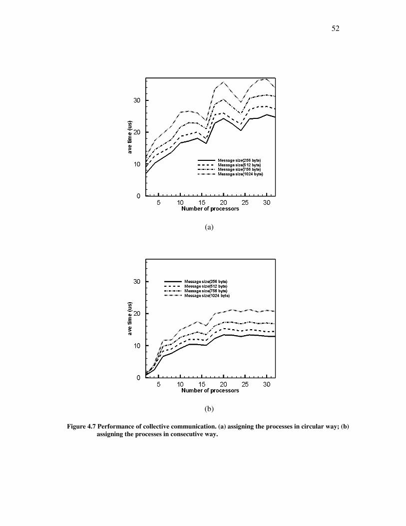
52

(a)

(b)

Figure 4.7 Performance of collective communication. (a) assigning the processes in circular way; (b)

assigning the processes in consecutive way.

53

5 PARALLEL IMPLEMENTATION OF PHASE FIELD

MODELING OF MAGNETIZATION PROCESS IN TERFENOL-D

CRYSTALS*

Terfenol-D has been the leading magnetostrictive material for magnetomechanical

transducers and actuators since its discovery in 1970’s.34

Because of its lower cost,

twinned crystals are usually used in technological applications.35

Twinned crystals are

grown along 112< >c direction and composed of alternate crystalline layers of twin

relation with c

111 plane whose normal is perpendicular to the 112< >c growth

direction.

Growth twinned Terfenol-D crystals have been studied over the past two decades.

However, the domain-level mechanisms are still not fully understood. This is because

the low magnetocrystalline anisotropy results in magnetization rotation that competes

with domain wall motion, and their interplay leads to complex domain-level processes.

Various models have been proposed to explain the magnetomechanical behaviors of

Terfenol-D, which are based on different mechanisms. Magnetic domain rotation model

assumes no interaction among different domains. The simulation of magnetization

*Part of this section reprinted with permission from “Phase field modeling of

magnetization process in growth twinned Terfenol-D crystals” by Y.Y.Huang and

Y.M.Jin, 2008. Applied Physics Letters, 93, 142504(3pp.). Copyright © 2009 American

Institute of Physics.

54

process is then reduced to the single magnetic domain rotation without considering the

domain wall motion. In the single magnetic domain rotation model, the process is

relative simple. The theoretical results are easy to calculate. In this case, the simulated

results by the parallel implementation will be compared with the theoretical results to

test our cluster and the parallel implementation.

However, the single magnetic domain rotation model is not able to realistically describe

the domain evolution in Tefenol-D. In fact, the magnetic and elastic interaction among

different domains will greatly affect the magnetic domain evolution. But the

computation related with the interaction is very complicated. No previous work has been

reported to properly take into account this important interaction. The phase field model

of magnetic materials in Section 2.1 can effectively evaluate the interaction effect with

the help of parallel computing on our developed workgroup cluster. The simulated

magnetization processes in twinned Terfenol-D crystal by our parallel implementation

will be presented as a successful application of the parallel computing for phase field

model of magnetic materials.

5.1 Simulation of single magnetic domain rotation

Figure 5.1(a) shows the initial spacial distribution of magnetization vectors in a single

magnetic domain. All magnetization vectors are oriented along the same easy axis. The

crystal structure is assumed to be twinning-free.

55

The physical properties of Terfenol-D used in our simulation are listed in Table 5.1. The

initial horizontal magnetization direction is corresponding to easy axis,[111]c. The

vertical direction, along which the magnetic field is applied, is [ 1 12]c in the crystal.

(a) (b)

(c) (d)

Figure 5.1 The magnetic domain temporal evolution under vertical external magnetic field. (a) time

steps=0; (b)time=100; (c) time =500; (d) time =1000.

56

Table 5.1 The physical properties of Terfenol-D used in the testing simulation

Ms, Saturation Magnetization 58 10 / m× A36,37

100λ , Magnetostriction 690 10 /mm mm−×

111λ 61640 10 /mm mm−× 36

1K , Magnetocrystalline Anisotropy 5 30.6 10 J / m− × 38

2K 52.0 10 J/m− × 38

YE , Yong’s modulus 30 Gpa39,40

µ , Shear modulus 11.5 Gpa

γ , Possion ratio 0.339,40

When an external magnetic field is applied along vertical direction, the magnetization

vectors will homogenously rotate and reorient to the easy axis closer to the direction of

external field. This magnetization process driven by the applied field, as the result of

minimizing total free energy, has been previously studied by domain theory.

Figure 5.1 shows the simulated results on the temporal evolution of magnetic domain

under 2000 Oe applied field along vertical direction. It is shown that the magnetization

vectors rotate and reorient to the [ 1 11]c easy axis, the closest easy axis to the applied

field. The simulation results predict same trend of magnetic domain evolution during

magnetization process as the theoretical prediction according to domain theory.

Besides the qualitative comparison between our simulation results and theoretical

prediction, an analytical solution for this case is also needed to verify the simulation

results quantitatively. A simple sequential program can give the correct quantitative

results for the magnetization process by tracking the magnetization vector corresponding

57

to the minimum energy. Following previous work on magnetic domain rotation model41

,

the simulation of a single magnetic domain rotation can be reduced to simulate the

behavior of a single magnetization vector under an external magnetic field, which is easy

to be calculated based on the principle of minimization of free energy. The sequential

code to implement this function is included in the Appendix C.

Figure 5.2 shows the comparison of magnetization curves simulated by the parallel

implementation of phase field model and a simple sequential program, respectively. The

exactly same results suggest that the parallel implementation on our cluster system is

functioning properly.

0 0.080.0480.0320.016 0.064

-0.5

0

0.5

1.0

Parallel program

Sequential program

sM/Η

Figure 5.2 Magnetization curve simulated by parallel implementation and a simple sequential

program.

58

5.2 Simulation of magnetization process in twinned single crystal

Most of the previous studies of magnetization processes in Terfenol-D crystal have

assumed no interaction among different magnetic domains in Terfenol-D35,37,41,42

. The

magnetic domain rotation without domain wall motion is considered to be the only

mechanism during magnetization process, which is against experimental observations.

Our parallel computing of the phase field model of magnetic materials will include the

magnetic and elastic interaction to quantitatively describe the magnetization processes

involving both magnetization rotation and domain wall motion in twinned Terfenol-D

crystals.

Figure 5.3 (a) illustrates an energy-minimizing domain configuration in growth twinned

Terfenol-D crystal, which is used as initial state of our simulations. The crystal consists

of alternate twin-related plate-shaped grains, and magnetization forms continuous 180°

domains across twin boundaries covering multiple grains, as shown in Figure 5.3 (a).

Figure 5.3 (b) illustrates the crystallographic orientations of a parent layer and its twin

layer, as well as the 111 c< > easy magnetization axes in respective layers. In the initial

state, magnetization vectors are aligned with easy axes throughout the crystal (i.e., VP1,

VP1′ in parent crystal and VT1, VT1′ in twin crystal), minimizing magnetocrystalline

energy. The domain continuity across twin boundaries makes them free of magnetic

charge and lattice misfit, minimizing magnetostatic and elastic energies. Such a domain

59

state is stable and is observed in experiments by applying a compressive stress along the

[112]c growth direction, and is the most desirable initial domain configuration because it

Figure 5.3 (a) Energy-minimizing domain configuration in growth twinned Terfenol-

D crystal. Magnetization vectors are aligned perpendicular to (111) growth

twin boundaries and form continuous 180°°°° domains. (b) Schematics of

crystallographic orientations and magnetization easy axes (projected to the

plane of figure) of a pair of twin-related crystals (parent and twin). Only

the easy axes whose dot products with applied magnetic field Hex along

c[112] growth direction are non-negative are shown.43

generates maximum field-induced deformation under magnetic field along [112]c

growth direction. It is worth noting that, starting from the initial state, complex domain

evolution processes take place in response to external magnetic field, where the

complexity results from the frustration in magnetic and elastic compatibilities at twin

boundaries. With increasing magnetic field applied along [112]c , magnetization vectors

tend to reorient to easy axes closer to [112]c , namely, VP2, VP3, VT2, and VT3. However,

60

the existence of twin boundaries leads to magnetic charge and lattice misfit there: among

the easy axes shown in Figure 5.3(b), besides of the initial state, only VP2/VT3 and

Vp3/VT2 are magnetically compatible, but they are elastically incompatible. As a result,

significant internal magnetic field and stress field develop, causing strong domain

interactions. We simulate the detailed domain evolutions to investigate the important

roles played by magnetic and elastic interactions in the magnetization processes. A

computation cell of 256×128 with grid size l=10nm and periodic boundary condition is

used to describe a representative Terfenol-D volume containing parent and twin grains

and initial 180° magnetic domains. The parameter used in the simulation is the same as

Table 5.1 lists.

The computer simulations reveal complex domain microstructure evolutions involving

both magnetization rotation and domain wall motion, and clarify the underlying domain

mechanisms responsible for the experimentally observed jump effect. In order to analyze

the respective contributions from magnetostatic interaction and elastic interaction, two

different cases are considered: (1) magnetically but not elastically interacting domains

with both magnetization rotation and domain wall motion, and (2) taking into account all

energy contributions and allowing magnetization to evolve freely. In both cases,

magnetic field is applied along [112]c .

The simulated magnetization curves are shown in Figure 5.4. A very large discontinuous

change is observed in both cases. This magnetization jump effects have been reported in

61

0 0.080.0480.0320.016 0.064

-0.5

0

0.5

1.0

sM/Η

Case (1)

Case (2)

Figure 5.4 Simulated magnetization curve in case (1) and (2).

experimental observation.38

The magnitude of the applied field corresponding to the

jump effect is called critical field. The critical field is an important parameter when

describe the magnetization behavior of Terfenol-D.

A detailed magnetic domain evolution during the magnetization process would help to

explain the magnetization jump effect. Figure 5.5 and Figure 5.6 show the magnetic

domain evolution in response to the applied field in case (1) and case (2), respectively.

62

-1 -0.5 0.50.0 1

M1

50 100 150 200 2500

40

80

120

050 100 150 200 2500

40

80

120

0

(a) (b)

50 100 150 200 2500

40

80

120

050 100 150 200 2500

40

80

120

0

(c) (d)

50 100 150 200 2500

40

80

120

050 100 150 200 2500

40

80

120

0

(e) (f)

50 100 150 200 2500

40

80

120

050 100 150 200 2500

40

80

120

0

(g) (h)

(h) Figure 5.5 Magnetic domain evolution for case (1). The vector plotted is the projection of

magnetization vector on the plane. The contour colors represent the magnetization vector

component out of the plane.

63

-1 -0.5 0.50.0 1

M2

50 100 150 200 2500

40

80

120

050 100 150 200 2500

40

80

120

0

(a) (b)

50 100 150 200 2500

40

80

120

050 100 150 200 2500

40

80

120

0

(b) (d)

50 100 150 200 2500

40

80

120

050 100 150 200 2500

40

80

120

0

(e) (f) Figure 5.6 Magnetic domain evolution for case (2). The vector plotted is the projection of

magnetization vector on the plane. The contour colors represent the magnetization vector

component in horizontal direction.

In case (1), the simulation observes nucleation and growth of VP2, VP3, VT2 and VT3

domains and finds that domain wall motion is the main mechanism producing one-step

jump as shown in Figure 5.5. During the magnetization jump, the domains are

magnetically compatible both inside grains (forming three-domain configurations

64

VP1/VP2/VP3, VT1/VT2/VT3, and two-domain configurations VP1′/VP3, VT1′/VT3) and

across twin boundaries (forming VP2/VT3 and VP3/VT2 neighboring pairs), which,

however, is elastically incompatible. Such domain structure is possible only in a system

where elastic interaction energy is significantly smaller than magnetocrystalline

anisotropy and magnetostatic interaction energies.

In case (2), the critical field is higher than that in case (1), as Figure 5.6 shows. The

higher critical field is due to the additional elastic constraint that necessitates a higher

field to activate nucleation and domain wall motion. More complicated domain

evolution is also observed in this case. But the phenomenon that domain wall motion

follows the initial magnetic domain rotation is observed both in case (1) and case (2).

Comparing the simulated domain evolution in case(1) and (2) with the single magnetic

domain rotation model in 5.1, we found that domain interactions through internal

magnetic and elastic fields greatly affect the predicted magnetization processes. Thanks

to the paralleling computing of phase field model based on our cluster system, we can

take into account these complicated interaction effects in order to accurately characterize

the magnetization of twinned Terfenol-D crystals, finding the underlying mechanisms

involve both domain wall motion and magnetization rotation.

65

6 CONCLUSIONS AND FUTURE WORK

According to the requirement of the parallel computing for phase field model of

magnetic materials, a workgroup cluster system with high performance network was

selected as the computation platform to support the parallel implementation. We have

successfully deployed the hardware system and configured the software environment to

build an 8-node workgroup cluster system, serving as a parallel computing platform for

MPI program. The 8-node workgroup cluster can simultaneously support a maximum of

32 processes for a MPI program to speed up the execution. The distributed memory

architecture in the cluster system accommodates 64 GB memory to support the parallel

computation usually involving huge data. And the high performance Myrinet network

greatly improves the performance of data communication among compute nodes.

Several testing programs have been implemented to evaluate the performance of the

cluster system, especially for the application of parallel computation using MPI. The

tested results show that the cluster system can efficiently execute MPI program with

intensive communication.

A simulation of the single magnetic domain rotation in Terfenol-D crystals was

performed by our parallel implementation of phase field model of magnetic materials on

the cluster system. The simulated results agree well with the theoretical prediction. A

further simulation including magnetic and elastic interaction using our parallel

implementation shows the important roles of these interaction effects in the

66

magnetization processes of twinned Terfenol-D crystals. This simulation example proves

that the paralleling computing for the phase field model of magnetic materials based on

the workgroup cluster system offers a promising tool for realistic domain analysis.

The developed computer cluster and parallel program lay the foundation for our planned

future work:

A. Analyze the output of benchmarking implementations to optimize the execution

of the MPI program;

B. Perform 3-D simulations of magnetization processes in Terfenol-D single and

polycrystals;

C. Simulate domain phenomena in other magnetic materials of interests.

67

REFERENCES

1 C. Kittel, Reviews of Modern Physics 21, 541-583 (1949).

2 A. Hubert and R. Schafer, Magnetic Domains: The Analysis of Magnetic

Microstructures (Springer, New York, 1998).

3 W. F.Brown, Micromagnetics (Krieger Pub Co, Malabar, FL, 1978).

4 H. H. Long, Z. J. Liu, E. T. Ong, and E. P. Li, in Micromagnetic Modeling

Simulations and Applications, (ETH Zentrum, Zurich, Switzerland, 2006), p.

398-401.

5 J. Fidler and T. Schrefl, Journal of Physics D: Applied Physics 33, 135-56 (2000).

6 H. J. Williams, R. M. Bozorth, and W. Shockley, Physical Review 75, 155-178

(1949).

7 L.-Q. Chen, Annual Review of Materials Research 32, 113-40 (2002).

8 S. Nambu and D. A. Sagala, Physical Review B: Condensed Matter 50, 5838-47

(1994).

9 A. Artemev, J. Slutsker, and A. L. Roytburd, IEEE Transactions on Ultrasonics,

Ferroelectrics and Frequency Control 55, 963-70 (2008).

10 S. Semenovskaya and A. G. Khachaturyan, Journal of Applied Physics 83, 5125

(1998).

11 R. Ahluwalia, T. Lookman, A. Saxena, and C. Wenwu, Applied Physics Letters

84, 3450-2 (2004).

12 T. M. Rogers, K. R. Elder, and R. C. Desai, Physical Review B: Condensed

Matter 37, 9638 (1988).

13 Y. M. Jin, A. Artemev, and A. G. Khachaturyan, Acta Materialia 49, 2309-20

(2001).

14 Y. Wang and A. G. Khachaturyan, Acta Materialia 45, 759-73 (1997).

15 A. Artemev, Y. Wang, and A. G. Khachaturyan, Acta Materialia 48, 2503-18

(2000).

68

16 W. J. Boettinger, J.A. Warren, C. Beckermann and A. Karma, Annual Review of

Materials Research 32, 163-194 (2002).

17 A. Karma and W. J. Rappel, Physical Review E: Statistical Physics, Plasmas,

Fluids, and Related Interdisciplinary Topics 53, 3017-20 (1996).

18 V. L. Ginzburg and L. D. Landau, Zhurnal Eksperimental'noi i Teoreticheskoi

Fiziki 20, 1064-82 (1950).

19 J. W. Cahn and J. E. Hilliard, Journal of Chemical Physics 31, 688-699 (1959).

20 L. Landau and E. Lifshitz, Physikalische Zeitschrift der Sowjetunion 8, 153-169

(1935).

21 Y. M. Jin, Y. U. Wang, A. Kazaryan, W. Yunzhi, D. E. Laughlin, and A. G.

Khachaturyan, Journal of Applied Physics 92, 6172-81 (2002).

22 J. X. Zhang and L. Q. Chen, Acta Materialia 53, 2845-55 (2005).

23 G. S. Almasi and A. Gottlieb, Highly Parallel Computing (Benjamin-Cummings

Publishers, Redwood City, CA, 1989).

24 D. Culler, J.P.Singh, P. Pacheco, and A. Gupta, Parallel Computing Set (Morgan

Kaufmann, San Francisco, CA, 1999).

25 A. E. Clark, J. D. Verhoven, O. D. McMasters, and E. D. Gibson, IEEE

Transactions on Magnetics 22, 973-5 (1986).

26 T. Sterling, D. J. Becker, and D. F. Savarese, How to Build a Beowulf: A Guide

to the Implementation and Application of PC Clusters (The MIT press,

Cambridge, MA, 1999).

27 D. G. Lord, V. Elliot, A. E. Clark, H. T. Savage, J. P. Teter, and O. D.

McMasters, IEEE Transactions on Magnetics 24, 1716-18 (1988).

28 M. Snir, S. Otto, S. Huss-Lederman, D. Walker, and J. Dongarra, MPI-The

Complete Reference (The MIT Press, Cambridge, MA, 1998).

29 R. C. Smith, S. Seelecke, M. M. Dapino, and Z. Z. Ounaies, Journal of the

Mechanics and Physics of Solids 54, 46-85 (2006).

30 S. Mani, R. Perez, L. Hyungoo, Z. Ounaies, W. Hung, and L. Hong, Transactions

of the ASME. Journal of Tribology 129, 836-40 (2007).

69

31 J. M. May, Parallel I/O for High Performance Computing (Morgan Kaufman,

San Francisco, CA, 2000).

32 Y. Wang, L. Q. Chen, and A. G. Khachaturyan, Acta Metallurgica et Materialia

41, 279-96 (1993).

33 W. Yunzhi, C. Long-Qing, and A. G. Khachaturyan, Journal of the American

Ceramic Society 79, 987-91 (1996).

34 D. C. Jiles, Journal of Physics D: Applied Physics 27, 1 (1994)

35 A. E. Clark, H. T. Savage, and M. L. Spano, IEEE Transactions on Magnetics 20,

1443-5 (1984)

36 D. C. Jiles and J. B. Thoelke, Journal of Magnetism and Magnetic Materials 134,

143-60 (1994).

37 W. D. Armstrong, Journal of Applied Physics 81, 2321-6 (1997).

38 A. E. Clark, J. P. Teter, and O. D. McMasters, Journal of Applied Physics 63,

3910-12 (1988).

39 Y. Zhou and F. G. Shin, IEEE Transactions on Magnetics 41, 2071-76 (2005).

40 W. D. Armstrong, Journal of Intelligent Material Systems and Structures 13, 137-

41 (2002).

41 W. Mei, T. Okane, and T. Umeda, Journal of Applied Physics 84, 6208-16

(1998).

42 R. D. James and D. Kinderlehrer, Journal of Applied Physics 76, 7012-14 (1994)

43 Y. Y. Huang and Y. M. Jin, Applied Physics Letters 93, 142504-06 (2008).

70

APPENDIX A. LIST OF HARDWARE IN THE 8-NODE APPLE

WORKGROUP CLUSTER

hardware description

Master node Xserve Quad Xeon server:

Two 2.66GHz Dual-Core Intel Xeon

8GB (8x1GB) memeory

750 GB Serial ATA ADM @ 7200-rpm hard drive

24x Combo (DVD-ROM/CD-RW)

Slave nodes Xserve Quad Xeon server:

Two 2.66GHz Dual-Core Intel Xeon

8GB (8x1GB) memeory

80 GB Serial ATA ADM @ 7200-rpm hard drive

24x Combo (DVD-ROM/CD-RW)

First management network 3Com 24-port Baseline Switch 2824 & cable

Second high performance

communication network

16-port Myrinet-2000 switch with Fiber ports and monitoring

8 Myrinet-2000 PCI-X NIC (2MB memory)

Myrinet-2000 fiber cable

Back up power supply APC Smart-UPS 1000VA USB & Serial Rack-Mount 1U 120V

Power supply APC 14-outlet, 15A, 0U PDU (AP9567)

Cooling system APC rack air removal unit

Enclosure APC NetShelter SX 42U Enclosure with Sides

71

APPENDIX B. INSTALLED SOFTWARE ON THE 8-NODE

APPLE WORKGROUP CLUSTER

Software installed Description

Mac OS X Serve Operating system, preinstalled by vendor

Apple Remote Desktop Remote administration tool

Absoft Pro Fortran 10.1 x86-32 OSX Commercial fortran compiler for Mac OS

X system

MX-2G A low-level message-passing system for

Myrinet networks

MPICH2-MX A port of MPICH2 ( an implementation of

MPI) on top of MX(ch_mx)

FFTW3 A free C subroutine library for computing

the discrete Fourier transform (DFT)

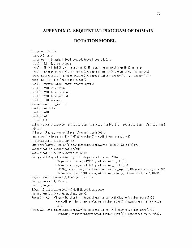
72

APPENDIX C. SEQUENTIAL PROGRAM OF DOMAIN

ROTATION MODEL Program rotation implicit none integer :: length,H_load_period,Record_period,i,n,j real:: k1,k2,time_step,p real:: M_initial(3),H_direction(3),H_load_increase(3),tmp,H(3),mh_tmp real:: Energy,Force(3),tmp_Force(3),Magnetization(3),Magnetization_sqrt(3) real,allocatable:: Energy_record(:),Magnetization_record(:,:),H_record(:,:) open(unit=11,file="Martensite.dat") read(11,*)time_step,length,record_period read(11,*)H_direction read(11,*)H_load_increase read(11,*)H_load_period read(11,*)M_initial Magnetization=M_initial read(11,*)k1,k2 read(11,*)H read(11,*)p close (11) allocate(Magnetization_record(3,length/record_period+1),H_record(3,length/record_period+1)) allocate(Energy_record(length/record_period+1)) tmp=sqrt(H_direction(1)**2+H_direction(2)**2+H_direction(3)**2) H_direction=H_direction/tmp tmp=sqrt(Magnetization(1)**2+Magnetization(2)**2+Magnetization(3)**2) Magnetization=Magnetization/tmp Magnetization_sqrt=Magnetization**2 Energy=k1*(Magnetization_sqrt(1)*Magnetization_sqrt(2)& +Magnetization_sqrt(2)*Magnetization_sqrt(3)& +Magnetization_sqrt(1)*Magnetization_sqrt(3))& +k2*Magnetization_sqrt(1)*Magnetization_sqrt(2)*Magnetization_sqrt(3)& -Magnetization(1)*H(1)-Magnetization(2)*H(2)-Magnetization(3)*H(3) Magnetization_record(:,1)=Magnetization Energy_record(1)=Energy do i=1,length if(mod(i,H_load_period)==0)H=H+H_load_increase Magnetization_sqrt=Magnetization**2 Force(1)=-2*k1*Magnetization(1)*(Magnetization_sqrt(2)+Magnetization_sqrt(3))& -2*k2*Magnetization(1)*Magnetization_sqrt(2)*Magnetization_sqrt(3)& +H(1) Force(2)=-2*k1*Magnetization(2)*(Magnetization_sqrt(1)+Magnetization_sqrt(3))& -2*k2*Magnetization(2)*Magnetization_sqrt(1)*Magnetization_sqrt(3)&

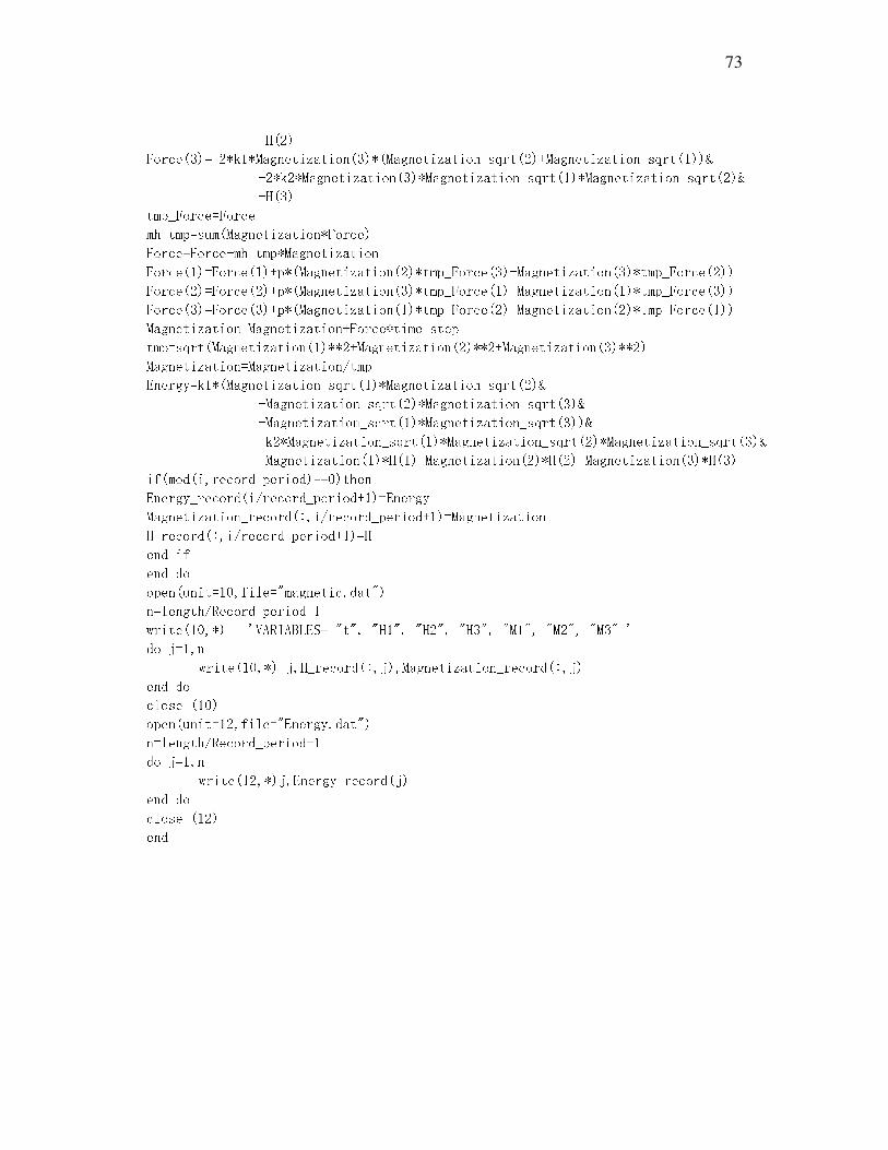
73

+H(2) Force(3)=-2*k1*Magnetization(3)*(Magnetization_sqrt(2)+Magnetization_sqrt(1))& -2*k2*Magnetization(3)*Magnetization_sqrt(1)*Magnetization_sqrt(2)& +H(3) tmp_Force=Force mh_tmp=sum(Magnetization*Force) Force=Force-mh_tmp*Magnetization Force(1)=Force(1)+p*(Magnetization(2)*tmp_Force(3)-Magnetization(3)*tmp_Force(2)) Force(2)=Force(2)+p*(Magnetization(3)*tmp_Force(1)-Magnetization(1)*tmp_Force(3)) Force(3)=Force(3)+p*(Magnetization(1)*tmp_Force(2)-Magnetization(2)*tmp_Force(1)) Magnetization=Magnetization+Force*time_step tmp=sqrt(Magnetization(1)**2+Magnetization(2)**2+Magnetization(3)**2) Magnetization=Magnetization/tmp Energy=k1*(Magnetization_sqrt(1)*Magnetization_sqrt(2)& +Magnetization_sqrt(2)*Magnetization_sqrt(3)& +Magnetization_sqrt(1)*Magnetization_sqrt(3))& +k2*Magnetization_sqrt(1)*Magnetization_sqrt(2)*Magnetization_sqrt(3)& -Magnetization(1)*H(1)-Magnetization(2)*H(2)-Magnetization(3)*H(3) if(mod(i,record_period)==0)then Energy_record(i/record_period+1)=Energy Magnetization_record(:,i/record_period+1)=Magnetization H_record(:,i/record_period+1)=H end if end do open(unit=10,file="magnetic.dat") n=length/Record_period+1 write(10,*) 'VARIABLES= "t", "H1", "H2", "H3", "M1", "M2", "M3" ' do j=1,n write(10,*) j,H_record(:,j),Magnetization_record(:,j) end do close (10) open(unit=12,file="Energy.dat") n=length/Record_period+1 do j=1,n write(12,*)j,Energy_record(j) end do close (12) end

74

VITA

Yongxin Huang, was born in Sichuan, China. He obtained his B.S. degree in Modern

Mechanics at University of Science and Technology of China in 2006. He came to Texas

A&M University to pursue his master degree with Dr. Yongmei Jin in fall 2006. The

author can be reached at iamhyx@tamu.edu. His contact address is:

Yongxin Huang

Texas A&M University

Department of Aerospace Engineering

H.R. Bright Building, Rm 701, Ross Street

College Station TX 77840