development of district-level agro-meteorological cotton ... · account for yield losses due to...
TRANSCRIPT

International Journal of Environmental Research and Development.
ISSN 2249-3131 Volume 6, Number 1 (2016), pp. 17-32
© Research India Publications
http://www.ripublication.com
Development of district-level Agro-meteorological
Cotton Yield Models in Punjab
Kalubarme Manik H.* and Saroha G.P.**
*Former Scientist, Space Applications Centre (ISRO), Ahmedabad
Currently, Bhaskaracharya Institute for Space Applications and
Geo-informatics (BISAG), Gandhinagar (Gujarat State)
** Computer Centre, Maharshi Dayanand University, Rohtak (Haryana State)
Abstract
District-level agromet-cotton yield models were developed using fortnightly
meteorological variables like mean maximum temperature (MXT), mean
minimum temperature (MNT) and total rainfall (TRF) from first fortnight of
June to First fortnight of November of every year for 24 years (1980-2003).
The crop condition (CC) term was also incorporated into the yield model to
account for yield losses due to pest/disease or drought conditions. This study
was conducted in the five major cotton producing districts namely Bathinda,
Faridkot, Firozpur, Mansa and Muktasar which account for 93.9 per cent of
acreage and 95.5 per cent of cotton production in Punjab State.Technology
trend has been separately modelled using time series data of district-level
cotton yield data of 24 years. Yield deviations from their respective trends
have been regressed against the selected subset of explanatory variables. The
weather variable subset for each district was selected by backward elimination
procedure based on the strength and significance of association observed from
the correlation matrix. The regression coefficients were tested for significance
at 95 percent confidence level using two tailed ‘t’ test. Repetitive analysis for
different districts has been facilitated by a semi-automated procedure based on
macros of different steps in data analysis.
The best sub-set of 3-4 explanatory agro-meteorological variables, which
resulted in highest R2 with minimum SEOE were selected for each district
independently. Using these set of variables cotton yields were predicted for
each district. The results indicate that the adjusted R2 for all the five districts
range from 0.91 to 0.95. This indicates that these variables explain around 91
to 95 per cent variability in the cotton yields in five districts. The most
significant variables in the regression equations of five districts are: Crop
Condition (CC), TRFJUN1, MNTOCT1 and MXTNOV1. The agro-

18 Kalubarme Manik H. and Saroha G.P.
meteorological model predicted and observed cotton yields in five districts
indicated that the relative deviations were in the range of-0.5 to 10 per cent in
all the districts from 1980 to 2003 period.
Key words: Agro-meteorological variables, Step-wise regression, Crop
Condition term, Relative Deviations, Mean Absolute Percent Error (MAPE),
1. INTRODUCTION
Cotton is one of the finest natural fibres available to mankind for clothing from time
immemorial. Cotton is an important commercial crop of the country and contributing
nearly 85% of the total domestic fibre consumption. It is estimated that cotton
requirement in India by 2025 will be around 140 lakh bales of lint and the present
production is around 123 lakh bales. India is the third largest cotton producer after
China and the United States of America. In terms of acreage India has largest cotton
acreage, accounting for 25 per cent of world acreage. However, India has the lowest
average yield (287 kg/ha against the world average of 567 kg/ha) amongst the major
cotton producing countries of the world.
1.1 Cotton growing regions in India
Cotton is mainly concentrated in four agro-ecological regions in India, either as a sole
or as an intercrop in cereal or pulse based cropping systems. Four species of cotton
grown in India, of which two are diploid (Gossypium arboreum and G. herbaceum)
and the other two tetraploids (G. hirsutum and G. barbadense). The diploid species
referred to as ‘Desi’ variety and accounts for 25-30 % of the production. These
varieties have low productivity and are not responsive to good agronomic practices in
terms of yield. In addition, its fibre is rough and short. However, the negligible cost of
desi cotton seeds accounts for its popularity amongst the poor farmers. The tetraploid
varieties account for the remaining 70% of the cotton production in India. These
varieties provide fine quality fibre, which is used by the textile industry. Although
hybrid seeds are costly, their yield can be as high as 800 kg/ha, depending on the
agronomic conditions. However, this too is lower than the 1200 kg/ha yield obtained
in the US.
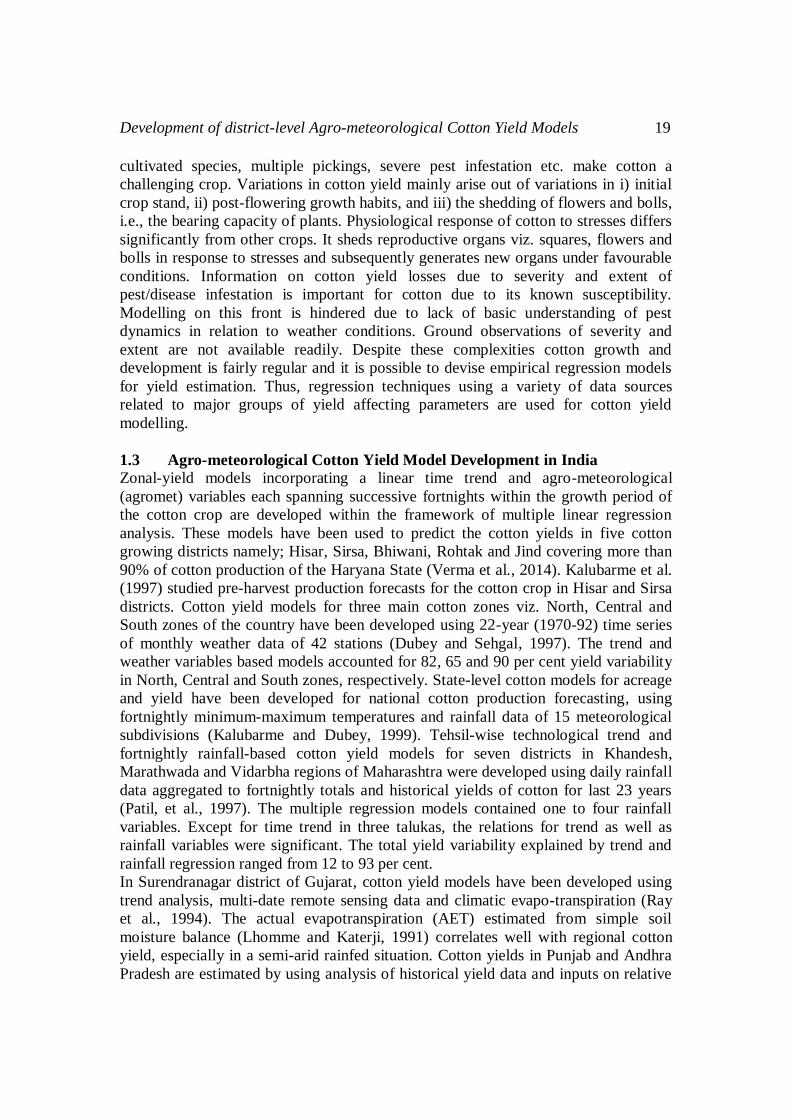
Cotton growing regions in India can be categorised into three major zones (Figure-1)
and nearly 99 per cent of cotton production in the country comes from first three
zones with Eastern zone contributing merely one per cent. The northern zone typically
produces 35 per cent of the total cotton produced in India, the central zone 40 per cent
and the southern zone 24 per cent. The northern zone is the primary producer of short
and medium staple cotton. These nine states are in first three zones, have distinct
characteristics in terms of soil base, varietal composition, irrigation practices, crop
rotations and intercrops, sowing and harvest periods and agro-climatic conditions,
which reflect on the realised yield levels and yield trends in respective zones.
1.2 Problems in Cotton Forecasting
Peculiarities like indeterminacy in growth habits, longer maturation period, multiple
Development of district-level Agro-meteorological Cotton Yield Models 19
cultivated species, multiple pickings, severe pest infestation etc. make cotton a
challenging crop. Variations in cotton yield mainly arise out of variations in i) initial
crop stand, ii) post-flowering growth habits, and iii) the shedding of flowers and bolls,
i.e., the bearing capacity of plants. Physiological response of cotton to stresses differs
significantly from other crops. It sheds reproductive organs viz. squares, flowers and
bolls in response to stresses and subsequently generates new organs under favourable
conditions. Information on cotton yield losses due to severity and extent of
pest/disease infestation is important for cotton due to its known susceptibility.
Modelling on this front is hindered due to lack of basic understanding of pest
dynamics in relation to weather conditions. Ground observations of severity and
extent are not available readily. Despite these complexities cotton growth and
development is fairly regular and it is possible to devise empirical regression models
for yield estimation. Thus, regression techniques using a variety of data sources
related to major groups of yield affecting parameters are used for cotton yield
modelling.
1.3 Agro-meteorological Cotton Yield Model Development in India
Zonal-yield models incorporating a linear time trend and agro-meteorological
(agromet) variables each spanning successive fortnights within the growth period of
the cotton crop are developed within the framework of multiple linear regression
analysis. These models have been used to predict the cotton yields in five cotton
growing districts namely; Hisar, Sirsa, Bhiwani, Rohtak and Jind covering more than
90% of cotton production of the Haryana State (Verma et al., 2014). Kalubarme et al.
(1997) studied pre-harvest production forecasts for the cotton crop in Hisar and Sirsa
districts. Cotton yield models for three main cotton zones viz. North, Central and
South zones of the country have been developed using 22-year (1970-92) time series
of monthly weather data of 42 stations (Dubey and Sehgal, 1997). The trend and
weather variables based models accounted for 82, 65 and 90 per cent yield variability
in North, Central and South zones, respectively. State-level cotton models for acreage
and yield have been developed for national cotton production forecasting, using
fortnightly minimum-maximum temperatures and rainfall data of 15 meteorological
subdivisions (Kalubarme and Dubey, 1999). Tehsil-wise technological trend and
fortnightly rainfall-based cotton yield models for seven districts in Khandesh,
Marathwada and Vidarbha regions of Maharashtra were developed using daily rainfall
data aggregated to fortnightly totals and historical yields of cotton for last 23 years
(Patil, et al., 1997). The multiple regression models contained one to four rainfall
variables. Except for time trend in three talukas, the relations for trend as well as
rainfall variables were significant. The total yield variability explained by trend and
rainfall regression ranged from 12 to 93 per cent.
In Surendranagar district of Gujarat, cotton yield models have been developed using
trend analysis, multi-date remote sensing data and climatic evapo-transpiration (Ray
et al., 1994). The actual evapotranspiration (AET) estimated from simple soil
moisture balance (Lhomme and Katerji, 1991) correlates well with regional cotton
yield, especially in a semi-arid rainfed situation. Cotton yields in Punjab and Andhra
Pradesh are estimated by using analysis of historical yield data and inputs on relative
20 Kalubarme Manik H. and Saroha G.P.
crop condition and varietal improvement (Anonymous, 1996). The models based on
remote sensing and meteorological data have been developed and used for cotton
yield forecasting in Gujarat and Maharashtra (Ray et al., 1999; Dubey and Chaudhary,
1995). Towards development of simple yield forecasting procedures, the time trend
has been used for yield estimation of different crops including cotton (Bhagia and
Dubey, 1994). Kharche (1984) has also validated Gossym simulation model for
growth and yield estimation of cotton. Role of rainfall and other climatic data for
cotton yield forecasting has been visualised and used in cotton yield forecasting
(Jahagirdar and Ratnalikar, 1995).
2. OBJECTIVES
Timely and accurate estimates of area and production of cotton with less subjectivity
would be highly useful in deciding the exportable surplus. Comprehensive, reliable
and timely data collection over extensive areas is the major problem. Therefore, in the
present study Subdivision-level weather data like minimum-maximum temperature
and rainfall has been analysed to develop agro-meteorological cotton yield models.
Agromet-yield models combining weather parameters have been generated for cotton
yield prediction in five major cotton growing districts in Punjab State. The broad
objective of this study is development of district-level Agro-meteorological yield
models in Punjab State.
3. MATERIALS AND METHODS
3.1 Study Area and its Location
The state of Punjab is one of the most intensively cultivated and irrigated areas of the
world. Area under agriculture is around 89 per cent of the total geographical area
(5.036 m ha) of the Punjab state with cropping intensity of 178 per cent, thus leaving
hardly any scope for further increase in area under agriculture. The success of
agricultural sector in Punjab state has very few parallels in the world. Scope for
horizontal expansion of agricultural land is limited but the scope for vertical
expansion for increasing productivity of lands already under cultivation with
improved technology is enormous. The Punjab State, with a geographical area of 50,
362 sq. km, forms a part of the Indus plain. It lies between 29o 33’ to 32
o 31’ N
latitude and 73o 53’ to 76
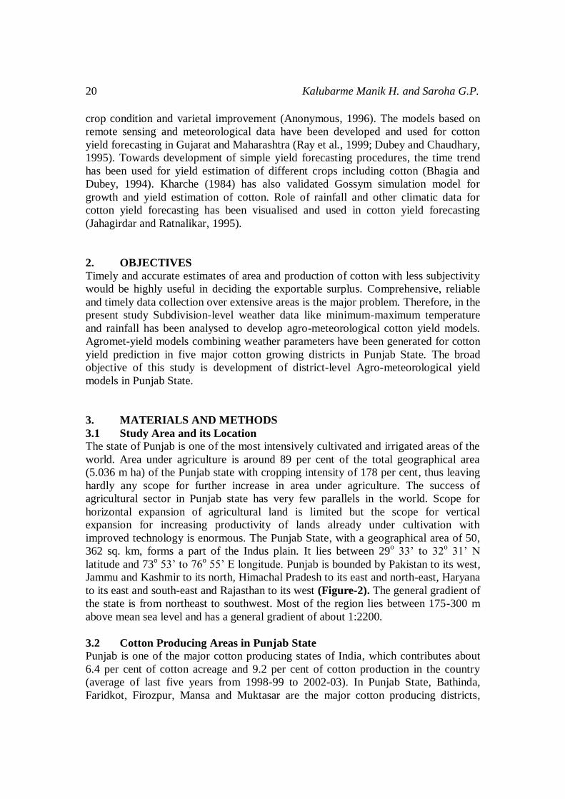
o 55’ E longitude. Punjab is bounded by Pakistan to its west,
Jammu and Kashmir to its north, Himachal Pradesh to its east and north-east, Haryana
to its east and south-east and Rajasthan to its west (Figure-2). The general gradient of
the state is from northeast to southwest. Most of the region lies between 175-300 m
above mean sea level and has a general gradient of about 1:2200.
3.2 Cotton Producing Areas in Punjab State
Punjab is one of the major cotton producing states of India, which contributes about
6.4 per cent of cotton acreage and 9.2 per cent of cotton production in the country
(average of last five years from 1998-99 to 2002-03). In Punjab State, Bathinda,
Faridkot, Firozpur, Mansa and Muktasar are the major cotton producing districts,
Development of district-level Agro-meteorological Cotton Yield Models 21
accounting for 93.9 per cent of acreage and 95.5 per cent of the cotton production of
the state (average of last five years from 1999-2000 to 2003-04). Cotton acreage and
production in Punjab State during Kharif 2003-2004 was 0.452 million hectares (mha)
and 1.478 million bales.
3.3 Data Used
3.3.1 Cotton Acreage, Yield and Production Statistics
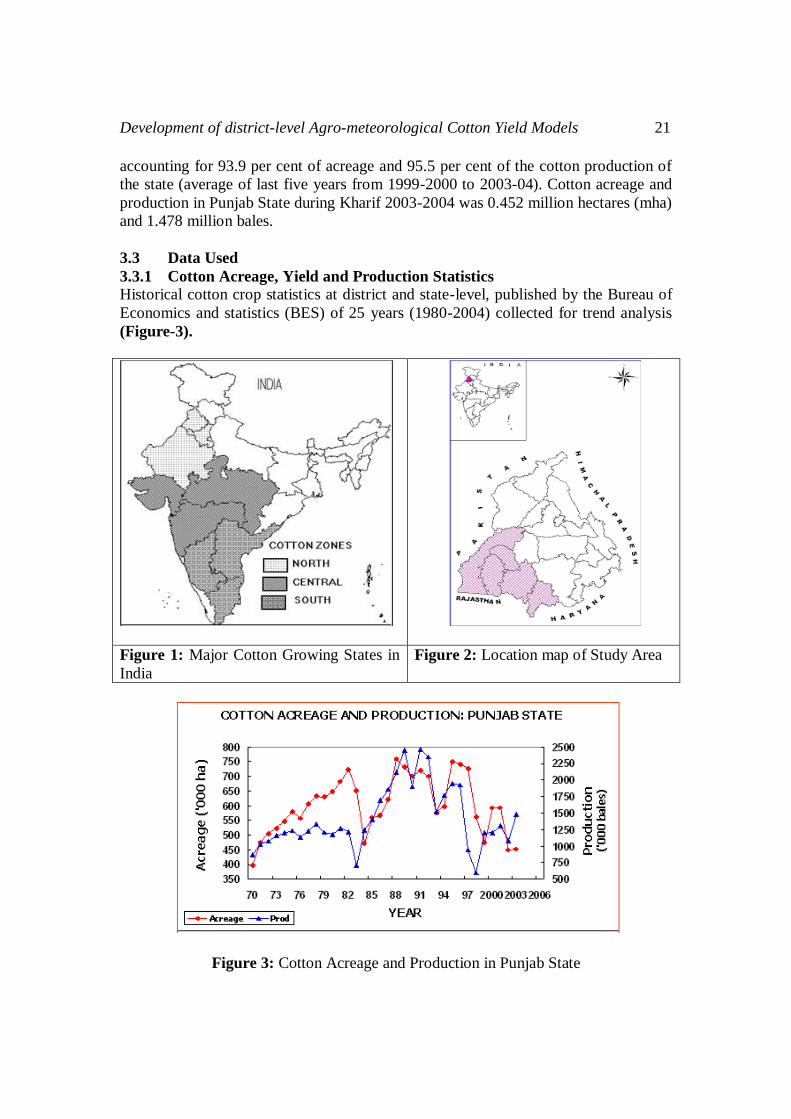
Historical cotton crop statistics at district and state-level, published by the Bureau of
Economics and statistics (BES) of 25 years (1980-2004) collected for trend analysis
(Figure-3).
Figure 1: Major Cotton Growing States in
India
Figure 2: Location map of Study Area
Figure 3: Cotton Acreage and Production in Punjab State
22 Kalubarme Manik H. and Saroha G.P.
3.3.2 Meteorological Data
Meteorological data like minimum temperature, maximum temperature, and rainfall
was collected from Bathinda meteorological observatory in the study area. The daily
meteorological data was compiled as fortnightly average values for the period of June
to December for developing district-level agrometeorological cotton yield models. In
case of rainfall data, instead of average values total rainfall during the fortnight was
computed.
3.3.3 Ground Truth Data
Field data at selected sites in the study districts was collected during the cotton
growing seasons. The field data collected includes variety, crop growth stage, crop
vigour, disease/insect-pest attack, soils, irrigation, fertilizer application, etc.
3.4 Data Analysis Procedure
3.4.1 Data Aggregation and Data-base Generation
The daily meteorological data like minimum-maximum temperatures (MNT-MXT),
and total rainfall (TRF) were aggregated over fortnightly values as independent
response variables. The first fortnight of May refers to average values of daily data
over May 1-15, while second fortnight of May (for example) refers to average values
of daily data over May 16-31; and likewise for other months from June to November.
The crop condition term computed from the historical yield data was also included in
the data series. This term takes into account the impact of yield reducing factors like
crop stresses (moisture stress, disease/pest stress etc.). Chakraborty, 1991 also
incorporated this crop condition term in the multiple regression for district-level
cotton yield forecast in Punjab State. The data was arranged in a matrix form where
each row refers to the data set of one year with columns as year, yield and fortnightly
meteorological values. Such data matrix was prepared for each district.
3.4.2 Semi-automated Procedure for Agro-meteorological Model Development
A Semi-automated procedure for development of cotton yield models based on trend
and fortnightly rainfall, maximum temperature (Tmax), and minimum temperature
(Tmin) was designed and developed. In this procedure, a set of command language
programs (macros) were written for semi-automated execution of model development
steps, in order to improve the efficiency of model development. A sequence of five
macros were written using development tools of spreadsheet (Quattro Pro) software
for following distinct steps of this procedure (Kalubarme, and Dubey, 1999), they are
as follows:
a) Data matrix generation: The data is arranged in a matrix form where each
row refers to the data set of one year with columns as year, fortnightly Tmax,
Tmin and rainfall and cotton yield.
b) Scatter plot creation for time trend: Year versus cotton yield line graph is
generated from the data matrix.
c) Computation of trend line and normalised yield deviations: Based on
observations of scatter plot, trend analysis and normalised deviations of yields
(NDY) are computed for one of the three options like Average, Single trend
Development of district-level Agro-meteorological Cotton Yield Models 23
and Two trends.
d) Correlation analysis and regression with backward elimination: A
correlation matrix of NDY and Tmax, Tmin and rainfall is generated and
subset of six best variables is selected on the basis of magnitude of correlation
coefficient.
e) Cotton yield prediction and its graphical presentation: Forecast of cotton
yield is generated using current season data and predicted values for current as
well as previous years are plotted on the original scatter plot.
3.4.3 Trend Analysis
For the purpose of trend analysis, 1970 was taken as reference year and the
subsequent years were referred to as modified years (Tm) where, Tm = (YEAR-1970)
and YEAR is 1971 for 1971-72 crop season. The scatter plots of year vs. yield have
been created for evaluating the time trend. Based on the assessment of scatter plots,
single or two-trend linear analysis is performed and appropriate regression equations
and their significance is obtained. However, if the regression line showed the
significant slope and the data points were uniformly distributed around this line, then
a single trend line was assumed to apply to the entire yield time series. The
significance of the slope of the equation was tested by using two-tailed t-test at 95%
confidence interval. The general form of the equation fitted is as follows (Kalubarme,
and Dubey, 1999):
Y = a + b * Tm
Where,
Y = seed cotton yield (kg/ha)
Tm = modified year i.e. (Year-1970)
a = intercept,
b = slope
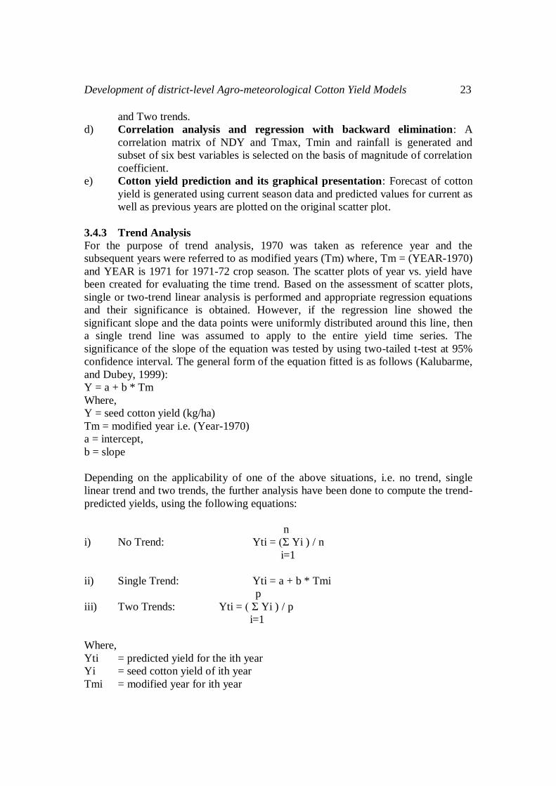
Depending on the applicability of one of the above situations, i.e. no trend, single
linear trend and two trends, the further analysis have been done to compute the trend-
predicted yields, using the following equations:
n
i) No Trend: Yti = (Σ Yi ) / n
i=1
ii) Single Trend: Yti = a + b * Tmi
p
iii) Two Trends: Yti = ( Σ Yi ) / p
i=1
Where,
Yti = predicted yield for the ith year
Yi = seed cotton yield of ith year
Tmi = modified year for ith year
24 Kalubarme Manik H. and Saroha G.P.
n, p = number of years used in model
a = intercept of trend line
b = coefficient of regression of trend line
3.4.4 Normalized Yield Deviations
Highly varying component of yield time series appears as transient around the trend
line. Normalised yield deviations representing these transients were computed and
related to the weather variables. The normalised yield deviation is absolute difference
of observed yield and the predicted yield from trend equation for a given year, which
is normalised with respect to predicted yield to take care of proportionate inter-annual
yield fluctuations. Trend predicted yield values are plotted against the observed yields
to assess the visual fit of model to data. The option giving the best fit is selected for
computation of normalised yield deviations using the following formula:
∆ Yi = Yti-Yoi
NDYi = ∆ Yi / Yti
= ( Yti-Yoi ) / Yti
Where,
∆ Yi = absolute yield deviation for ith year
Yti = trend predicted yield from trend for ith year
Yoi = observed yield for the ith year
NDYi = normailized deviations of yield for ith year, with respect to long term trend
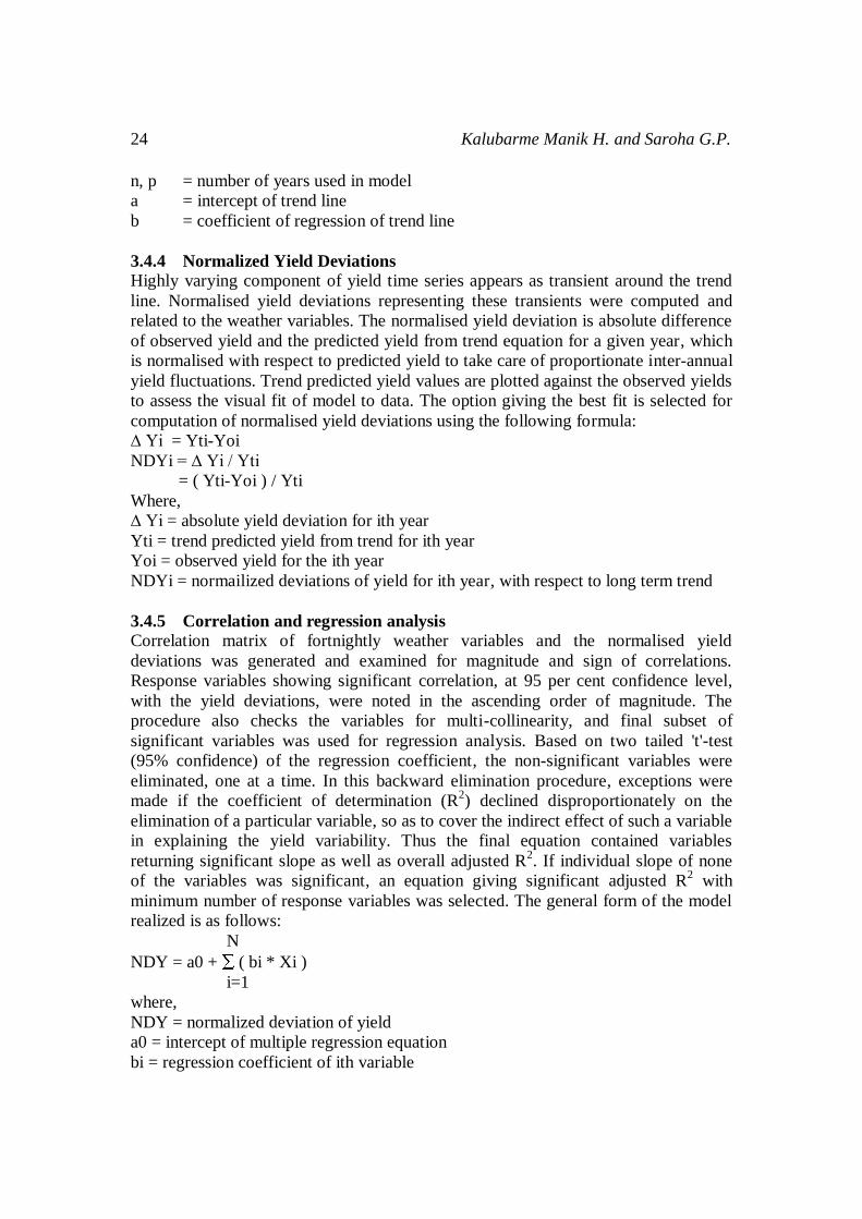
3.4.5 Correlation and regression analysis
Correlation matrix of fortnightly weather variables and the normalised yield
deviations was generated and examined for magnitude and sign of correlations.
Response variables showing significant correlation, at 95 per cent confidence level,
with the yield deviations, were noted in the ascending order of magnitude. The
procedure also checks the variables for multi-collinearity, and final subset of
significant variables was used for regression analysis. Based on two tailed 't'-test
(95% confidence) of the regression coefficient, the non-significant variables were
eliminated, one at a time. In this backward elimination procedure, exceptions were
made if the coefficient of determination (R2) declined disproportionately on the
elimination of a particular variable, so as to cover the indirect effect of such a variable
in explaining the yield variability. Thus the final equation contained variables
returning significant slope as well as overall adjusted R2. If individual slope of none
of the variables was significant, an equation giving significant adjusted R2 with
minimum number of response variables was selected. The general form of the model
realized is as follows:
N
NDY = a0 + ( bi * Xi )
i=1
where,
NDY = normalized deviation of yield
a0 = intercept of multiple regression equation
bi = regression coefficient of ith variable
Development of district-level Agro-meteorological Cotton Yield Models 25
Xi = ith fortnightly weather (response) variable
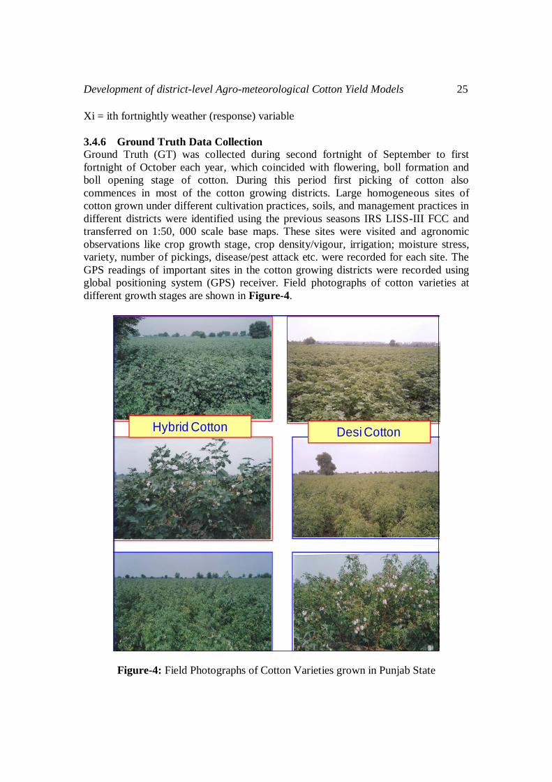
3.4.6 Ground Truth Data Collection
Ground Truth (GT) was collected during second fortnight of September to first
fortnight of October each year, which coincided with flowering, boll formation and
boll opening stage of cotton. During this period first picking of cotton also
commences in most of the cotton growing districts. Large homogeneous sites of
cotton grown under different cultivation practices, soils, and management practices in
different districts were identified using the previous seasons IRS LISS-III FCC and
transferred on 1:50, 000 scale base maps. These sites were visited and agronomic
observations like crop growth stage, crop density/vigour, irrigation; moisture stress,
variety, number of pickings, disease/pest attack etc. were recorded for each site. The
GPS readings of important sites in the cotton growing districts were recorded using
global positioning system (GPS) receiver. Field photographs of cotton varieties at
different growth stages are shown in Figure-4.
Field Photographs of Hybrid and Desi Cotton varieties grown in Punjab
Desi Cotton Hybrid Cotton
Figure-4: Field Photographs of Cotton Varieties grown in Punjab State

26 Kalubarme Manik H. and Saroha G.P.
4. RESULTS AND DISCUSSIONS
4.1 Trend Predicted Cotton Yields
The scatter plots of year vs. cotton yields for five districts were generated to assess the
fluctuations and trends in cotton yields over the years. It was observed that the cotton
yields were highly fluctuating over the period of 24 years in cotton growing districts
of Punjab State depending upon the climatic conditions and incidence of pest/disease.
During the kharif seasons from 1984 to 1996, cotton yields in all the districts were
between 400 to 650 kg/ha and showed an increasing trend. However, cotton yields
during the periods of 1980 to 1983 and 1997 to 2002 were below 400 kg/ha and
cotton seasons of 1983, 1997 and 1998 showed drastic reductions in cotton yields and
were below 250 kg/ha in all the cotton growing districts. A single trend was fitted to
the yield time series data for all the districts and trend predicted yields were
computed. The scatter plot of observed yields along with trend predicted yields for
one of the districts (Bathinda) is given in Figure-5.
Figure-5: Trend Predicted Cotton Yields in Bathinda District of Punjab State
4.2 Correlation and regression analysis with backward elimination
The trend predicted yields in all the districts were used to compute normalized yield
deviations. The computed yield deviations were regressed against the fortnightly
meteorological variables like mean maximum temperature (MXT), mean minimum
temperature (MNT) and total rainfall (TRF) from first fortnight of June to First
fortnight of November of every year for 24 years (1980-2003). The data-set of yield
deviations along with Crop Condition (CC) term and meteorological variables
generated for one of the districts (Bathinda) is shown in Table-1.
From the correlation matrix of yield deviations and meteorological variables a subset
of top eight variables showing significant correlations, at 95 % confidence level, with
yield deviations was selected for further regression analysis (Table-2). In the multiple

Development of district-level Agro-meteorological Cotton Yield Models 27
regression analysis of eight variable with yield deviations, the non-significant
variables were eliminated, one at a time, by backward elimination procedure based on
two tailed ‘t’-test (95% confidence).
Table-1: Correlation data set generated for Agromet-Yield model development in
Bathinda
Table-2: A subset of eight variables selected for regression analysis of Bathinda
District
28 Kalubarme Manik H. and Saroha G.P.
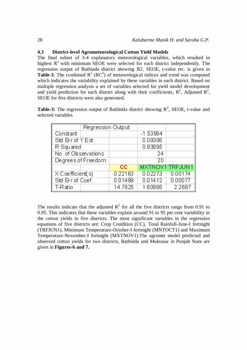
4.3 District-level Agrometeorological Cotton Yield Models
The final subset of 3-4 explanatory meteorological variables, which resulted in
highest R2 with minimum SEOE were selected for each district independently. The
regression output of Bathinda district showing R2, SEOE, t-value etc. is given in
Table-3. The combined R2 (RC
2) of meteorological indices and trend was computed
which indicates the variability explained by these variables in each district. Based on
multiple regression analysis a set of variables selected for yield model development
and yield prediction for each district along with their coefficients, R2, Adjusted R
2,
SEOE for five districts were also generated.
Table-3: The regression output of Bathinda district showing R2, SEOE, t-value and
selected variables
The results indicate that the adjusted R2 for all the five districts range from 0.91 to
0.95. This indicates that these variables explain around 91 to 95 per cent variability in
the cotton yields in five districts. The most significant variables in the regression
equations of five districts are: Crop Condition (CC), Total Rainfall-June-I fortnight
(TRFJUN1), Minimum Temperature-October-I fortnight (MNTOCT1) and Maximum
Temperature-November-I fortnight (MXTNOV1).The agromet model predicted and
observed cotton yields for two districts, Bathinda and Muktasar in Punjab State are
given in Figures-6 and 7.

Development of district-level Agro-meteorological Cotton Yield Models 29
Figure-6: Agromet Model Predicted Cotton Yields in Bathinda District, Punjab State
Figure-7: Agromet Model Predicted Cotton Yields in Muktasar District, Punjab State
4.4 Performance Evaluation of District-level Agrometeorological Cotton-
Yield Models
The performance of district-level Agrometeorological cotton-yield models developed
using both meteorological variables in terms of their yield prediction capability was
evaluated by computing Mean Absolute Per cent Error (MAPE) in comparison with

30 Kalubarme Manik H. and Saroha G.P.
yields estimated by the Department of Agriculture, Government of Punjab. The
MPAE of one of the districts (Bathinda) during 1980 to 2003 period are presented in
Table-4.
Table-4: Observed and Predicted Cotton Yields along with MAPE for Bathinda
District
Year Cotton Yield (kg/ha) Relative DeviObserved Predicted (%)
1980 339 326 -3.81981 356 342 -3.91982 304 320 5.31983 206 222 7.81984 443 447 0.91985 426 442 3.81986 516 520 0.81987 490 482 -1.61988 452 446 -1.31989 577 559 -3.11990 489 457 -6.51991 647 652 -0.81992 577 559 -3.11993 495 489 -1.21994 521 552 6.01995 451 455 0.91996 449 450 0.21997 245 249 1.21998 173 159 -8.11999 314 350 11.52000 383 372 -2.92001 395 377 -4.62002 472 467 -1.12003 546 555 1.8
MAPE -0.2
Mean Absolute Percent Error (MAPE) = 100*Pr1
YldObs
YldObsedYld
N
It can be seen from Table-4 that in general, the MAPE of the predicted yields are
within 10 per cent, except for one data point of 1999. The agro-meteorological model
predicted and observed cotton yields in all the five districts indicated that the relative
deviations were in the range of-0.5 to 10 per cent in all the districts from 1980 to 2003
period.

Development of district-level Agro-meteorological Cotton Yield Models 31
CONCLUSIONS
This study was conducted in the five major cotton producing districts namely
Bathinda, Faridkot, Firozpur, Mansa and Muktasar which account for 93.9 per cent of
acreage and 95.5 per cent of cotton production in Punjab State. In this study Agro-
meteorological yield modelling approach was adopted to develop district-level cotton
yield models using Agro-meteorological data of past 25-years.
District-level cotton yield models were developed using fortnightly
meteorological variables like mean maximum temperature (MXT), mean
minimum temperature (MNT) and total rainfall (TRF) from first fortnight of
June to First fortnight of November of every year for 24 years (1980-2003).
The crop condition term was also incorporated into the yield model to account
for yield losses due to pest/disease or drought conditions. Technology trend
has been separately modelled using time series data of district-level cotton
yield data of 24 years. Yield deviations from their respective trends have been
regressed against the selected subset of explanatory variables.
The weather variable subset for each district was selected by backward
elimination procedure based on the strength and significance of association
observed from the correlation matrix. The regression coefficients were tested
for significance at 95 percent confidence level using two tailed ‘t’ test.
Repetitive analysis for different districts has been facilitated by a semi-
automated procedure based on macros of different steps in data analysis.
The best sub-set of 3-4 explanatory agro-meteorological variables, which
resulted in highest R2 with minimum SEOE were selected for each district
independently. Using these set of variables cotton yields were predicted for
each district. The results indicate that the adjusted R2 for all the five districts
range from 0.91 to 0.95. This indicates that these variables explain around 91
to 95 per cent variability in the cotton yields in five districts.
The most significant variables in the regression equations of five districts are:
Crop Condition (CC), TRFJUN1, MNTOCT1 and MXTNOV1. The agro-
meteorological model predicted and observed cotton yields in five districts
indicated that the relative deviations were in the range of-0.5 to 10 per cent in
all the districts from 1980 to 2003 period.
REFERENCE
1. Anonymous, 1996. Cotton Acreage and Condition Assessment (CACA):
Project Proposal for Phase-II. RSAM/SAC/CACA/PP/18/96, Space
Applications Centre, Ahmedabad.
2. Bhagia, N. and Dubey, R.P., 1994. Yield modelling of cotton and sorghum
using time series analysis. Scientific Note: RSAM/SAC/CAPE-II/SN/35/94,
Space Applications Centre, Ahmedabad, 53.
3. Chakraborty, M., 1992. In Status Report of Cotton Acreage and Condition
Assessment Project.RSAM/SAC/CACA/SR/01/92. Space Applications Centre
(ISRO), Ahmedabad-53.
32 Kalubarme Manik H. and Saroha G.P.
4. Dubey, R.C., Chaudhary, A., and Kale, J.D., 1995. The estimation of cotton
yield based on weather parameters in Maharashtra. Mausam, 46(3): 275-278.
5. Dubey, R.P. and Sehgal, V.K., 1997. Development of weather based zonal
models for cotton crop in India. Paper presented at INTROMET (International
Symposium on Advances in Tropical Meteorology) under theme, “Monsoon
and Management of Agricultural activities, IIT, New Delhi, Dec. 2-5, 1997.
6. Jahagirdar, S.W. and Ratnalikar, D.V., 1995. Cotton yield model based on
monthly rainfall and rainy days. Paper submitted to the Research Review Sub-
committee, P.K.V., Akola.
7. Kalubarme, M.H., Hooda, R.S., Yadav, Manoj, Saroha, G.P., Arya, V.S.,
Bhatt, H.P., Ruhal, D.S., Khera, A.P., Hooda, I.S. and Singh, C.P., 1998.
Cotton production forecast using remote sensing data and agro-meteorological
yield models in Haryana. Paper presented in National seminar on,
‘Applications of Remote Sensing and GIS for sustainable development’, Nov.
26-28, 1997, NRSA, Hyderabad.
8. Kalubarme, M.H., and Dubey, R.P., 1999. State-level agro-meteorological
models for national cotton production forecast. Scientific Note:
RSAM/SAC/FASAL-TD/SN/05/99, Space Applications Centre, Ahmedabad.
9. Kalubarme, M.H., Yadav, Manoj, Ruhal, D. S., Khera, A. P. and Hooda, I.S.,
1997. Agro-meteorological cotton yield modelling in Haryana, Paper
presented in TROPMET 97: Monsoon, Climate and Agriculture, Bangalore,
February 10-14.
10. Kharche, S.G., 1984. Simulation models on growth and yield of cotton. A
Dissertation submitted to the faculty of Mississippi State University for award
of Ph.D. Degree in Agronomy.
11. Lhomme, J.P. and Katerji, N., 1991. A simple modeling of crop water balance
for agrometeorological applications. Ecological Modeling, 57, 11-25.
12. Patil, S.M., Sehgal, V.K., Mehta, N.S., Shrivastava, S.K., Dubey, R.P. and
Nalamwar, R.V., 1997. Taluqwise technology trend and rainfall based cotton
yield models for seven districts in Khandesh, Marathwada and Vidarbha
regions of Maharashtra. Scientific Note: RSAM/SAC/CAPE-II/SN/72/97.
13. Ray, S.S., Pokharna, S.S. and Ajai, 1994. Cotton production estimation using
IRS-1B and meteorological data. Int. J. Remote Sens., 15(5): 1085-1090.
14. Ray, S.S., Pokharna, S.S. and Ajai, 1999. Cotton yield estimation using agro-
meteorological model and satellite-derived profile. Int. J. Remote Sensing,
1999, Vol. 20, No. 14, 2693-2702.
15. Verma, U., Piepho, H.P., Ogutu, J.O., Kalubarme, M.H. and Goyal, M., 2014.
Development of agromet models for district-level cotton yield forecasts in
Haryana State. International J. of Agricultural and Statistical Sciences, 10(1),
59-65.