DEVELOPMENT OF HPGE DETECTORFOR THE LONGITUDINAL EMITTANCE MEASUREMENT

By

Reiko Taki

A THESIS

Submitted toMichigan State University

in partial fulfillment of the requirementsfor the degree of

MASTER OF SCIENCE

Department of Physics and Astronomy

2003

ABSTRACT

DEVELOPMENT OF HPGE DETECTORFOR THE LONGITUDINAL EMITTANCE MEASUREMENT

By

Reiko Taki

The longitudinal emittance of the beam from the RIKEN Ring Cyclotron (RRC) is

indispensable knowledge for the operation of the Radioactive Isotope Beam Factory,

which is now under construction and uses the RRC as an injector. We proposed to

employ a HPGe detector as a compact and convenient energy detector for longitudinal

emittance measurements and studied the feasibility of its use with high-energy heavy

ions. A reasonably good energy resolution, δE/E = 6.5×10−4, has been observed for

1890-MeV 14N, which makes the HPGe promising. A new detector is being fabricated

to achieve a better resolution. Also the longitudinal emittances were measured for

3800-MeV 40Ar and 2420-MeV 22Ne. It has been demonstrated that the measurement

of longitudinal emittance provides rich information on the acceleration condition, such

as the single-turn extraction and the effect of phase compression, and is very helpful

for the beam tuning of the present and new facilities.

TABLE OF CONTENTS

1 Introduction 1

1.1 Purpose of Experiment . . . . . . . . . . . . . . . . . . . . . . . . . . 1

1.2 Cyclotron . . . . . . . . . . . . . . . . . . . . . . . . . . . . . . . . . 2

1.2.1 Principle of Cyclotron . . . . . . . . . . . . . . . . . . . . . . 3

1.2.2 Sector Focus Cyclotron . . . . . . . . . . . . . . . . . . . . . . 5

1.2.3 Beam Extraction . . . . . . . . . . . . . . . . . . . . . . . . . 7

1.2.4 Single- and Multi-Turn Extraction . . . . . . . . . . . . . . . 10

1.2.5 Longitudinal Emittance . . . . . . . . . . . . . . . . . . . . . 11

1.2.6 Phase Compression . . . . . . . . . . . . . . . . . . . . . . . . 13

1.3 HPGe Detector . . . . . . . . . . . . . . . . . . . . . . . . . . . . . . 13

1.3.1 Range of Particles . . . . . . . . . . . . . . . . . . . . . . . . 14

1.3.2 Simple Estimation of Energy Resolution . . . . . . . . . . . . 15

1.3.3 Energy Loss Straggling . . . . . . . . . . . . . . . . . . . . . . 16

1.3.4 Recombination Effect . . . . . . . . . . . . . . . . . . . . . . . 19

1.3.5 Radiation Damage . . . . . . . . . . . . . . . . . . . . . . . . 19

2 Experimental Arrangement 20

i

2.1 AVF Cyclotron . . . . . . . . . . . . . . . . . . . . . . . . . . . . . . 21

2.2 Ring Cyclotron . . . . . . . . . . . . . . . . . . . . . . . . . . . . . . 22

2.3 Beam Transport . . . . . . . . . . . . . . . . . . . . . . . . . . . . . . 24

2.4 Target and Collimator . . . . . . . . . . . . . . . . . . . . . . . . . . 27

2.5 Magnetic Spectrometer SMART . . . . . . . . . . . . . . . . . . . . . 28

2.6 Detector Systems . . . . . . . . . . . . . . . . . . . . . . . . . . . . . 31

2.6.1 Energy Resolution Measurement . . . . . . . . . . . . . . . . . 31

2.6.2 Longitudinal Emittance Measurements . . . . . . . . . . . . . 32

2.7 Data Acquisition . . . . . . . . . . . . . . . . . . . . . . . . . . . . . 35

2.7.1 Energy Resolution Measurement . . . . . . . . . . . . . . . . . 35

2.7.2 Longitudinal Emittance Measurements . . . . . . . . . . . . . 37

3 Analysis 38

3.1 Energy Calibration of HPGe . . . . . . . . . . . . . . . . . . . . . . . 38

3.2 Veto by Active Slit . . . . . . . . . . . . . . . . . . . . . . . . . . . . 41

3.3 Time Calibration . . . . . . . . . . . . . . . . . . . . . . . . . . . . . 42

3.4 Position Calibration . . . . . . . . . . . . . . . . . . . . . . . . . . . 42

3.5 Time of Flight Correction . . . . . . . . . . . . . . . . . . . . . . . . 44

4 Results and Discussions 50

4.1 Energy Resolution of HPGe . . . . . . . . . . . . . . . . . . . . . . . 50

4.2 Longitudinal Emittance of 40Ar Beam— case of single turn extraction — . . . . . . . . . . . . . . . . . . . 52

4.3 Longitudinal Emittance of 22Ne Beam— case of multi-turn extraction — . . . . . . . . . . . . . . . . . . . 58

ii

5 Conclusions 62

6 Future Prospects 64

Appendix 66

A Angular Distribution of Elastic Scattering 67

iii

LIST OF TABLES

1.1 Ranges of Ge for typical beams delivered from the RRC. . . . . . . . 15

1.2 Estimation of energy loss straggling for some materials. . . . . . . . 18

2.1 List of the experiments. . . . . . . . . . . . . . . . . . . . . . . . . . 20

2.2 Accelerator parameters. . . . . . . . . . . . . . . . . . . . . . . . . . 24

2.3 Energy spreads due to the angular acceptance of the collimator ∆Eang

and the energy-loss straggling in the target ∆Estraggle (FWHM). . . . 28

2.4 Typical optical characteristics of the SMART. . . . . . . . . . . . . . 29

3.1 Energies of γ rays emitted by 60Co, 22Na, 137Cs and 40Kr, and thecorresponding ADC channels. . . . . . . . . . . . . . . . . . . . . . . 40

4.1 Peak width in observed energy spectra, the contributions from energy-loss straggling and the intrinsic energy resolution of HPGe at normaland 43 injections for 1890-MeV 14N. . . . . . . . . . . . . . . . . . 51

6.1 Specifications of Ge detector (Princeton Gammatech: IGP1010185Model). . . . . . . . . . . . . . . . . . . . . . . . . . . . . . . . . . . 65

iv

LIST OF FIGURES

1.1 Schematic layout of the new facility, RIBF, at RIKEN. . . . . . . . . 1

1.2 Schematic drawings of the cyclotron. Vertical (left) and horizontal(right) mid plane cross sections. . . . . . . . . . . . . . . . . . . . . 3

1.3 Schematic drawings of AVF (upper panel) and Ring (lower panel) cy-clotrons at RIKEN. Both of them have four sectors. . . . . . . . . . 6

1.4 Beam current versus radius measured with the differential probe for a135-MeV/A 28Si14+ beam at the RRC. . . . . . . . . . . . . . . . . . 9

1.5 Kinetic energy versus RF phase near extraction (solid curve) and en-ergy profile of the extracted beam for the case of multi-turn extraction(dots). . . . . . . . . . . . . . . . . . . . . . . . . . . . . . . . . . . 10

1.6 (T, t) correlation of 185-MeV Ar beam measured at VICKSI (presentlyISL), Hahn-Meitner Institute [4]. The right panel shows a high-resolutionmeasurement (presumably, labels on abscissa, 84.8 and 85.0, shouldread 184.8 and 185.0). . . . . . . . . . . . . . . . . . . . . . . . . . . 11

1.7 (T, φ) correlation of the extracted beam for the case of single-turnextraction. Injection phases are displaced by 0, ±3 and ±6 aroundφ0. . . . . . . . . . . . . . . . . . . . . . . . . . . . . . . . . . . . . . 12

2.1 Schematic layout of RIKEN Accelerator Research Facility. . . . . . . 21

2.2 Dependence of acceleration voltage on the relative phase φ. . . . . . 22

2.3 Beam configuration in the RRC in the case of the AVF injection. . . 24

2.4 Transport line components from the RRC to F2 of SMART togetherwith the extraction components of the RRC. . . . . . . . . . . . . . 25

v

2.5 A Typical beam envelope from the RRC to the target of scatteringchamber in E4 experimental area. . . . . . . . . . . . . . . . . . . . 26

2.6 Side view of the SMART scattering chamber. . . . . . . . . . . . . . 27

2.7 Arrangement of SMART and the detector system. . . . . . . . . . . 30

2.8 Setup of the HPGe detector and the slits for the energy resolutionmeasurement. . . . . . . . . . . . . . . . . . . . . . . . . . . . . . . . 31

2.9 Setup of Si-PSD and the plastic scintillators for the longitudinal emit-tance measurements. . . . . . . . . . . . . . . . . . . . . . . . . . . . 33

2.10 A simplified equivalent circuit and the layout of Si-PSD. . . . . . . . 34

2.11 Data acquisition system for the energy resolution measurement. . . . 36

2.12 Data acquisition system for the longitudinal emittance measurements. 36

3.1 Energy spectra from 137Cs, 22Na and 60Co sources which are used forthe energy calibration of ADC channels. The peak from the back-ground, 40K, was also observed. . . . . . . . . . . . . . . . . . . . . . 39

3.2 Energy spectra for all events (unshaded) and for events without signalsfrom the active slit (shaded). . . . . . . . . . . . . . . . . . . . . . . 41

3.3 Typical time spectrum used for time calibration (upper panel). Pulsesfrom a time calibrator had a 10 ns interval over 100 ns range. Theregression line is shown in the lower panel. . . . . . . . . . . . . . . 42

3.4 Spectrum used for calibration of Left ADC (upper panel). The regres-sion line is shown in the lower panel. . . . . . . . . . . . . . . . . . . 43

3.5 Qleft-Qright plot for different x generated by the dedicated position cal-ibrator. The inset is a closeup around the intersecting point. . . . . 44

3.6 Spectrum of x/L calculated by using Eq. (2.5) (upper panel). Discretepeaks reflecting the strip structure are clearly seen. The lower panelshows the regression curve to deduce the correct position determinedby the least squares method. . . . . . . . . . . . . . . . . . . . . . . 45

3.7 Time spectra with the first-term correction only. The injection phasewith respect to the RF phase of the RRC, ∆φinj, is displaced in stepof 2. . . . . . . . . . . . . . . . . . . . . . . . . . . . . . . . . . . . 47

vi

3.8 Same as Fig. 3.7but with the correction assuming (l|δ) = −35.5 cm/%. 47

3.9 The correlation between the time and momentum of particles detectedat F2 without the stripper (left) and with the stripper (right). . . . . 48

3.10 Beam spot on a ZnS scintillation target at the target position with(right panel) and without the stripper foil (left panel). Ticks on thetarget are marked in 5 mm step. . . . . . . . . . . . . . . . . . . . . 49

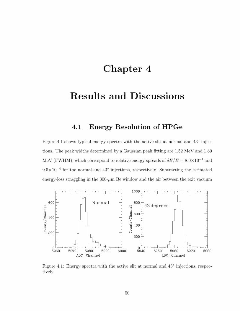
4.1 Energy spectra with the active slit at normal and 43 injections, re-spectively. . . . . . . . . . . . . . . . . . . . . . . . . . . . . . . . . 50

4.2 Longitudinal emittances of 3800-MeV 40Ar. The injection phase ∆φinj

is displaced relative to the RF of the RRC in step of 2. . . . . . . . 53

4.3 Schematic illustration of phase compression effect for the case of narrow-bunched beam. The extraction time is either relative to the RF of theRRC (upper panel) or relative to the injection (lower panel). . . . . 55

4.4 Projected spectra of the extraction time relative to the injection. Thephase of the RF with respect to the injection, ∆φinj, is shifted in stepof 2. . . . . . . . . . . . . . . . . . . . . . . . . . . . . . . . . . . . 56

4.5 Shifts of time spectra deduced from Fig. 4.4 plotted as a function of∆φinj. The solid line is a prediction from Eq. (1.13). The dashed curveis a third order polynomial for eye-guide. . . . . . . . . . . . . . . . 57

4.6 Time spectrum (upper panel), the longitudinal emittances for the mainand adjacent turns at the nominal Dee voltage (middle panels) and ata slightly lowered Dee voltage (lower panels). Straight lines are foreye-guide. . . . . . . . . . . . . . . . . . . . . . . . . . . . . . . . . . 59

4.7 Schematic illustration of δT -δt correlations for neighboring turns atthe nominal Dee voltage (upper panel) and at a slightly lowered Deevoltage (lower panel). . . . . . . . . . . . . . . . . . . . . . . . . . . 60

6.1 Overview of the newly fabricated HPGe detector. . . . . . . . . . . . 65

A.1 Angular distribution of 197Au(14N,14 N)197Au elastic scattering at E/A =135 MeV/A compared with Rutherford scattering. The exponentialline is for eye-guide. . . . . . . . . . . . . . . . . . . . . . . . . . . . 68

vii

Chapter 1

Introduction

1.1 Purpose of Experiment

The new facility, Radioactive Isotope Beam Factory (RIBF), is now under construc-

tion at RIKEN and is scheduled to be operational in 2006. The schematic layout of

the facility is shown in Fig. 1.1. The main accelerator of the present facility, RIKEN

Ring Cyclotron (RRC), will be used as a pre-accelerator in this new facility. The

typical injection energy is 60 MeV/A, although the RRC is capable to accelerate up

RARF Heavy-ion accelerator system

RIBF RI beam experimentswill be started in 2006.

RIBF Exp. Bldg.

SRC

fRC

BF2

BigRIPSIRC

BF1

RI Beam Factory (RIBF): Upgrading project of RIKEN Accelerator Research Facility (RARF)

RFQ

RILAC

AVF

RRCRIBF Accle. Bldg.

Figure 1.1: Schematic layout of the new facility, RIBF, at RIKEN.

1

to 135 MeV/A for Z/A = 1/2 particles.

For designing new accelerator components, such as a re-buncher after the RRC,

the information of time structure and energy spread, i.e., the longitudinal emittance of

the beam coming from the RRC is needed. For successful operation of this accelerator

complex, it is also important to know the longitudinal emittance while beam tuning.

Because the typical time and relative energy spreads of the beam coming from the

RRC are 1 ns and 10−3, the required time and energy resolutions for the measurement

are δt ' 0.1 ns and δE/E ' 10−4, respectively. Such an energy resolution is usually

achieved by using a magnetic spectrometer, but, for the routine beam tuning, the

use of a compact and convenient detector system is more desirable. We propose to

employ a High Purity Germanium (HPGe) detector for this purpose. The response of

HPGe to medium energy protons, ≤ 150 MeV, was reported, for example in Ref. [10],

but that to energetic heavy ions is not well known. In the present experiment, the

energy resolution of HPGe has been studied for 135-MeV/A 14N, the momentum of

which is defined by using a magnetic spectrometer. We also studied the longitudinal

emittances of 95-MeV/A 40Ar and 110-MeV/A 22Ne beams.

1.2 Cyclotron

Cyclotron is a circular particle accelerator first built by Lawrence and Livingston in

1930. The cyclotron employs a uniform magnetic field to guide particles along the

circular orbit, so that particles can be accelerated many times by the same acceler-

ating cavities. The principle of the cyclotron, however, is limited to non-relativistic

particles because of the change of revolution frequency. The technique of varying the

radio frequency (RF) of the accelerating cavity overcomes this limitation. This is the

principle of synchrocyclotron. In 1938, a significant breakthrough, strong focusing,

came out from H. A. Thomas. He found that the radial dependence of the magnetic

2

V = VD cos ωD t

B

Dee

Figure 1.2: Schematic drawings of the cyclotron. Vertical (left) and horizontal (right)mid plane cross sections.

field makes the revolution frequency of particles constant. The machine employing

this principle is called isochronous cyclotron. In contrast to the synchrocyclotron,

the isochronous cyclotron provides a continuous thus high-intensity beam. Presently,

most of cyclotrons are isochronous type. Details of cyclotrons as well as other types

of accelerators can be found in textbooks, e.g., Refs. [1] and [2].

1.2.1 Principle of Cyclotron

The schematic configuration of an early cyclotron is shown in Fig. 1.2. The cyclotron

consists of magnets which generate a uniform magnetic field and two accelerating

cavities which extend over the whole aperture between the poles. These cavities form

semi-circles and generate the accelerating fields between them. Because of its shape,

the cavity is often called Dee. Since particles travel inside Dees, they are contained

in a vacuum box. The magnets have coils surrounding their poles and yokes which

reduce leakage field and resistance of magnetic field.

A particle which has the charge q and is moving at the velocity of v in the electric

and magnetic fields, E and B, feels the Lorentz force,

F = q (E + v ×B) . (1.1)

Particles injected from the center of the cyclotron perpendicularly to the uniform

3

magnetic field B are guided along a circular orbit. Under this condition, Eq. (1.1) is

reduced to

F = qvB .

An equilibrium between Lorentz force and the centrifugal force,

mγv2

r= qvB ,

defines the curvature of the orbit r as

r =p

qB, (1.2)

where m and p are the mass and momentum of the particle, respectively. γ is the

Lorentz factor defined by γ = 1/√

1−(v/c)2. Particles are accelerated by an electric

field E every time when passing the gap between the accelerating cavities. Because

the momentum of the particle p increases after acceleration, the curvature of the orbit

r becomes larger and larger. Accordingly, the orbit of the particle forms in spiral.

The revolution time τ and the revolution frequency frev are given by

τ =2πr

v=

2π

qB

p

v=

2πmγ

qB=

1

frev

. (1.3)

They remain constant for non-relativistic case, where γ ' 1. The accelerating voltage

V (t) applied to the cavities is a sinusoidal function,

V (t) = VD cos ωDt . (1.4)

The angular velocity ωD = 2πfrf is chosen in such a way that the particles get the

4

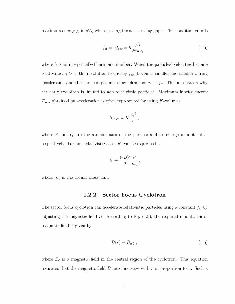
maximum energy gain qVD when passing the accelerating gaps. This condition entails

frf = hfrev = hqB

2πmγ, (1.5)

where h is an integer called harmonic number. When the particles’ velocities become

relativistic, γ > 1, the revolution frequency frev becomes smaller and smaller during

acceleration and the particles get out of synchronism with frf. This is a reason why

the early cyclotron is limited to non-relativistic particles. Maximum kinetic energy

Tmax obtained by acceleration is often represented by using K-value as

Tmax = KQ2

A,

where A and Q are the atomic mass of the particle and its charge in units of e,

respectively. For non-relativistic case, K can be expressed as

K =(rB)2

2

e2

mu

,

where mu is the atomic mass unit.

1.2.2 Sector Focus Cyclotron

The sector focus cyclotron can accelerate relativistic particles using a constant frf by

adjusting the magnetic field B. According to Eq. (1.5), the required modulation of

magnetic field is given by

B(r) = B0γ , (1.6)

where B0 is a magnetic field in the central region of the cyclotron. This equation

indicates that the magnetic field B must increase with r in proportion to γ. Such a

5

Figure 1.3: Schematic drawings of AVF (upper panel) and Ring (lower panel) cy-clotrons at RIKEN. Both of them have four sectors.

6

field, however, causes a vertical defocusing of particles, while it provides a horizontal

focusing. This vertical instability can be compensated by an azimuthally alternating

varying field. Focusing powers arise at the boundaries between strong and week fields.

These fields can be formed by hill and valley on the poles. This type of machine is

called azimuthally varying field (AVF) cyclotron (upper panel of Fig. 1.3). The larger

difference of field strength makes the stronger focusing power. In order to provide

a maximumly varying field, the magnets are divided into some sectors as shown in

lower panel of Fig 1.3. Accelerating cavities are arranged in the field-free regions,

where much more spaces are available than magnet regions. Thus the cavities can be

designed to have higher quality factors and generate the RFs with higher voltages.

The orbit of particles becomes quadrangle-like because the particles go straight in the

field-free regions while they curve in the magnetic fields. The average of magnetic

fields in each turn,

〈B(r)〉 =1

2π

∫ 2π

0

B(r, θ)dθ ,

must satisfy Eq. (1.6) to keep the isochronal condition, where θ is the azimuth.

1.2.3 Beam Extraction

Several kinds of extraction methods are employed for cyclotrons [3]. Generally in

the case of positive ion acceleration, the beams can be extracted with the help of

extraction devices such as electrostatic and magnetic deflector channels (EDC and

MDC). The EDC consists of a septum, which is a thin inner electrode at the earth

potential, and an outer electrode at a negative high potential. Reaching the final

radius, particles enter between the septum and the outer electrode to be directed

away from the cyclotron magnetic field. In order to reduce the cyclotron magnetic

field along the extraction path, MDCs are employed. In the design of MDC, it is

7

important to keep the stray magnetic field as small as possible in the area of the

last acceleration orbit. For achieving a high extraction efficiency and a good beam

quality, a large separation between successive turns is desired. The radial position of

a particle at an azimuth θ in the cyclotron is given by

r(θ) = r0(θ) + x(θ) sin(νrθ + θ0) , (1.7)

where r0(θ) is the radial position of the equilibrium orbit at that azimuth, x(θ) is

the radial oscillation amplitude and θ0 is an arbitrary phase angle. νr is a betatron

tune defined as the number of cycles of the radial oscillation during one turn. For

incoherent oscillations, the amplitude x(θ) is given by

√βr0(θ)εx ,

where βr0 is the radial beta function for radius r0 and at azimuth θ, and εx the radial

emittance. Rewriting Eq. (1.7) as a function of turn number n, the radial position at

a fixed azimuth θi = 2πn becomes

r(θi) = r0(θi) + x(θi) sin(2πn(νr−1) + θ0) , (1.8)

where for convenience νr−1 has been taken since νr is close to 1, which is the case

with most isochronous cyclotrons. The separation between two successive turns is

given by

∆r(θi) = ∆r0(θi) + ∆x sin(2πn(νr−1) + θ0)

+2π(νr−1)x cos(2πn(νr−1) + θ0) . (1.9)

8

The first term on the right-hand side in Eq. (1.9) represents the orbit separation due

to acceleration. Using the kinetic energy of particle T =√

(mc2)2+(pc)2−mc2 and

Eq. (1.2), the turn separation due to acceleration becomes

∆r

r=

γ

γ + 1

∆T

T, (1.10)

where r and ∆T are the average radius and the energy gain per turn, respectively.

The second term in Eq. (1.9) gives the orbit separation by an increase in the oscilla-

tion amplitude. This can be accomplished by providing a gradient of first harmonic

magnetic field, which leads to an increase in the beta function βr0 . This method is

called regenerative extraction. The third term in Eq. (1.9) describes a turn separation

due to precessional orbit motion with the oscillation amplitude x. The maximum turn

separation produced by the precessional motion is given by 2π(νr−1)x. The extrac-

tion using the precessional orbit motion is called precessional extraction. It can be

achieved by off-center injection, which generates a rotation of the orbit center around

the machine center, and thus, the oscillation pattern of the radius. A typical turn

separation is presented in Fig. 1.4.

Figure 1.4: Beam current versus radius measured with the differential probe for a135-MeV/A 28Si14+ beam at the RRC.

9

1.2.4 Single- and Multi-Turn Extraction

In general, particles with a different value of the accelerating RF phase experi-

ence a different number of turns before reaching the extraction radius. In a purely

isochronous cyclotron, RF phase of a particle remains constant. This leads to the

multi-turn extraction. The single-turn extraction can be achieved by restricting the

injection RF phase with a help of phase slits in the central region of cyclotron. This

reduces the energy spread of the extracted beam. The flat-top technique is also use-

ful, as described later. The kinetic energy T and the radius r of a particle on an ideal

orbit with accelerating voltage V (t) in Eq. (1.4) are

T (φ) = T0 cos φ ' T0

(1− 1

2φ2

)(1.11)

r(φ) = r0

√T (T+2mc2)

T0(T0+2mc2)' r0

[1− 1

2

γ

γ+1φ2

],

where T0 and r0 are the kinetic energy and radius at the central RF phase φ0, and φ is

the phase difference with respect to φ0. Figure 1.5 shows the energies for orbits near

Figure 1.5: Kinetic energy versus RF phase near extraction (solid curve) and energyprofile of the extracted beam for the case of multi-turn extraction (dots).

10

extraction and the energy pattern of the extracted beam as a function of RF phase.

It is seen that several turns get extracted when an energy gate opens between T1

and T2, which are mainly defined by the EDC and MDC apertures. The single-turn

extraction can be accomplished by restricting phase width ≤ φ2−φ1. This is further

discussed for an actual case in Sec. 4.3.

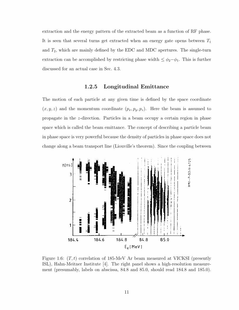
1.2.5 Longitudinal Emittance

The motion of each particle at any given time is defined by the space coordinate

(x, y, z) and the momentum coordinate (px, py, pz). Here the beam is assumed to

propagate in the z-direction. Particles in a beam occupy a certain region in phase

space which is called the beam emittance. The concept of describing a particle beam

in phase space is very powerful because the density of particles in phase space does not

change along a beam transport line (Liouville’s theorem). Since the coupling between

Figure 1.6: (T, t) correlation of 185-MeV Ar beam measured at VICKSI (presentlyISL), Hahn-Meitner Institute [4]. The right panel shows a high-resolution measure-ment (presumably, labels on abscissa, 84.8 and 85.0, should read 184.8 and 185.0).

11

Figure 1.7: (T, φ) correlation of the extracted beam for the case of single-turn extrac-tion. Injection phases are displaced by 0, ±3 and ±6 around φ0.

the transverse and longitudinal motion, as well as the coupling between the horizontal

and vertical plane, is being ignored in linear beam dynamics, six-dimensional phase

space can be split into three independent two-dimensional phase planes. In systems

where the beam energy stays constant, the slopes of the trajectory a≡ px/p and

b≡ py/p may be used instead of the transverse momenta and the transverse emittances

are usually defined as areas in x-a and y-b planes. Likewise the longitudinal emittance

is defined as an area in z-p plane or, as another set of canonically conjugate variables,

in t-T plane. The area alone, however, does not reflect the detailed quality of the

beam thus we will rather discuss the longitudinal distribution in t-T plane.

The beam extracted from the cyclotron is expected to have a quadratic correlation

between T and φ, or equivalently time t, according to Eq. (1.11). Such a correlation

was actually measured at several facilities [4, 5]. An example at VICKSI (presently

ISL), Hahn-Meitner Institute, is shown in Fig. 1.6.

The phase width of the injection beam is often reduced by using a phase slit

and a buncher so that the single-turn is extracted easily. In this case, the quadratic

correlation is not observed, but it is useful to intentionally displace the injection phase

to see the correlation and to diagnose the acceleration condition conveniently (Fig.

1.7). This method is employed in the present experiment for 40Ar case (Sec. 4.2).

12

1.2.6 Phase Compression

The phase compression was first mentioned by Muller and Mahrt [6] and generalized

in Ref. [7]. A radial voltage distribution of the RF cavity produces a time varying

magnetic field. This field compresses the bunch size of beam for a radially increasing

voltage or expands it for a radially decreasing voltage. For an ideal isochronous

cyclotron, the effect of phase compression can be described by the Hamiltonian

H(T (n), φ(n)) = qV (n) sin φ(n) ,

where φ(n) is the relative phase and qV (n) is the peak energy gain per turn at n-th

turn. Since the Hamiltonian H does not depend explicitly on the turn number n

(∂H/∂n = 0), it is a constant of motion. This leads to an important relation between

peak energy gain and relative phase of acceleration,

qV (n1) sin φ(n1) = qV (n2) sin φ(n2) , (1.12)

where n1 and n2 are turn numbers in an isochronous cyclotron. According to this

equation, a voltage distribution increasing from Vinj at injection to Vext at extraction

can compress the original phase spread φinj into

φext =Vinj

Vext

φinj . (1.13)

1.3 HPGe Detector

In this section, matters related to operation of HPGe detectors are described. Detailed

review of them can be found in textbooks, e.g., Refs. [8] and [9].

13

1.3.1 Range of Particles

Heavy charged particles lose their energy by Coulomb interaction with the electrons

and the nuclei of absorbing materials. The collisions of heavy charged particles with

the free and bound electrons of the material are mainly responsible for the energy

loss of heavy particles and result in the ionization or excitation of the atom. The

scattering from nuclei also occurs, although not as often as electron collisions. Thus

the major part of the energy loss is due to electron collisions. The average energy

loss per unit path length,dE

dx, was calculated by Bethe and Bloch. The Bethe-Bloch

formula is

−dE

dx= 2πNar

2emec

2ρZ

A

z2

β2

[ln

(2meγ

2v2Wmax

I2

)− 2β2

], (1.14)

where

2πNar2emec

2 = 0.1535 MeV cm2/g

Na : Avogadro’s number = 6.022 ×1023 mol−1

re : classical electron radius = 2.817×10−23 cm

me : electron mass = 0.511 MeV/c2

Z : atomic number of absorbing material

A : atomic weight of absorbing material

ρ : density of absorbing material

z : charge of incident particle in units of e

Wmax ' 2mec2η2 : maximum energy transfer in a single collision

β =v

cof the incident particle

η = βγ .

14

The mean range of a particle with a given energy E0 is obtained by integrating the

inverse of Bethe-Bloch formula over E,

R(E0) =

∫ E0

0

(dE

dx

)−1

dE . (1.15)

The ranges in Ge for some typical beams calculated by Eq. (1.15) are listed in Table

1.1. The result indicates that the HPGe detector with thickness of 1 cm, which is

easily obtained commercially, can stop the beams of 60 MeV/A and serve as an energy

detector for the present purpose.

Table 1.1: Ranges of Ge for typical beams delivered from the RRC.

E/A = 135 MeV/AParticle Energy Range

[MeV] [cm]α 540 3.798

12C6+ 1620 1.26514N7+ 1890 1.08416O8+ 2160 0.949

20Ne10+ 2700 0.76028Si14+ 3780 0.54640Ar18+ 5400 0.477

E/A = 60 MeV/AParticle Energy Range

[MeV] [cm]α 240 0.920

12C6+ 720 0.30714N7+ 840 0.26316O8+ 960 0.231

20Ne10+ 1200 0.18628Si14+ 1680 0.13640Ar18+ 2400 0.122

1.3.2 Simple Estimation of Energy Resolution

The intrinsic energy resolution δε depends on the number of electron-hole pairs pro-

duced by incoming beam and the Fano factor. Assuming that all the energy deposited

by radiation E is used to create electron-hole pairs and that the number of those pairs

n follows the Poisson distribution, the expected relative energy resolution δε/E can

be obtained by

δε

E= 2.35

√F

n= 2.35

√Fw

E, (1.16)

15

where n = E/w and w is the average energy for electron-hole creation, which is 2.96 eV

for Ge at 77 K. The Fano factor F is still not well determined, but is about 0.12. The

total energy resolution δE contains contributions from other sources, e.g., electronics

noise and fluctuation of leakage current. Denoting them by D, the resolution can be

expressed as

δE =√

δε2 + D2 . (1.17)

A simple estimation of energy resolution is obtained by neglecting D and by us-

ing certification values given in catalogs of commercial products. For example, the

DGP100-15 planer-type Ge detector of EURISIS MEASURES Inc., a typical charged-

particle detector with thickness of 15 mm and sensitive area of 100 mm2, has an energy

resolution of δE0 = 20 keV (FWHM) for α particles with E0 = 5.486 MeV. On the

assumption that δε0 = δE0, the relative energy resolution for 1890-MeV 14N becomes

δε

E=

√E0

E

δε0

E0

= 1.96×10−4 (FWHM) .

This value makes HPGe very promising for the present purpose.

1.3.3 Energy Loss Straggling

In the measurement of heavy ions, one of major source of D is the energy loss strag-

gling in the entrance window of the detector, typically made of Be, and in other

materials which particles pass through. The amount of energy loss is not equal to the

mean energy loss because of the statistical fluctuations in the number of collisions of

charged particles with electrons and in the energy transferred in each collision. There-

fore, after passing through a fixed thickness of material, an initially mono-energetic

beam has an energy distribution. Calculating the distribution of energy losses for a

given thickness of absorber is generally divided into two cases: thick absorbers and

16

thin absorbers.

For relatively thick absorbers, where the number of collisions is large, the total

energy loss distribution will approach the Gaussian form,

f(x, ∆) ∝ exp

[−(∆− ∆)2

2σ2

],

where x is the thickness of the absorber, ∆ is the energy loss in the absorber, ∆ is the

mean energy loss, and σ is the standard deviation. In the case of relativistic heavy

ions, the spread σ of this Gaussian can be calculated by

σ2 =

(1− 1

2β2

)

1− β2σ2

0 and (1.18)

σ20 = 4πNar

2e(mec

2)2ρZ

Ax = 0.1569ρ

Z

Ax [MeV2] , (1.19)

where σ0 is the spread of the Gaussian for non-relativistic heavy ions, Na is Avogadro’s

number, re and me are the classical electron radius and mass, and ρ, Z and A are the

density, atomic number and atomic weight of the absorber, respectively.

For thin absorbers or gases, where the number of collisions is small, the distribu-

tion of energy loss is complicated to calculate because of the possibility of large energy

transfers in a single collision. Since a long tail is added to the high energy side of

the energy loss probability distribution, the mean energy loss no longer corresponds

to the peak. One basic calculation of this distribution was carried out by Vavilov.

According to Vavilov’s theory, the spread σ is given by

σ2 =ξ2

κ

1− β2

2, (1.20)

where κ = ∆/Wmax and ∆ ' ξ = 2πNar2emec

2ρZ

A

z2

β2x, which is the approximated

mean energy loss obtained by taking only the first term and ignoring the logarithmic

term in Eq. (1.14). Vavilov’s formula agrees with Eq. (1.18) for heavy particles.

17

Substituting κ and ξ to Eq. (1.20), σ is reduced to

σ = C z , where

C =

[2πNar

2em

2ec

4ρZ

Ax

] 12

.

The energy loss straggling caused in a thin absorber is in proportion to the charge

of incident particle, but independent of the injecting energy E. Thus the relative

energy spread σ/E becomes larger with E decreasing. It may be useful to rewrite the

formula as

σ

E= C

z

Ain

/E

Ain

.

Thus, for incident particles having the same injection energy per nucleon and the

same charge-to-mass ratio z/Ain, the relative energy spread becomes constant.

Table 1.2: Estimation of energy loss straggling for some materials.

Energy thickness δE/E[MeV/A] [µm] = 2.35σ/E

Be window135 300 0.38×10−3

135 25 0.11×10−3

60 25 0.25×10−3

Plastic Scintillator135 100 0.18×10−3

60 100 0.41×10−3

Table 1.2 shows the energy loss straggling estimated for some materials. The

plastic scintillator is used as a timing detector. Since its contribution is relatively large

even with a thickness as thin as 100 µm, the use of a micro-channel plate combined

with a thin foil for secondary electron production may be considered. Contributions

from the vacuum window (Mylar, aramid, etc.), as well as the gold target which is

used for elastic scattering, must be also taken into consideration.

18

1.3.4 Recombination Effect

Another possible source of D in Eq. (1.17) is the recombination effect. In the measure-

ment of heavy ions, the high density of charge carriers created along the ion tracks can

decrease the local electric field for charge collection, thus increase the magnitude of

the electron-hole recombination. A method usually employed for reducing the pulse

height defect caused by this is to increase the bias voltage. However, the leakage

current, which will be increased by the radiation damage described in the next sec-

tion, may limit the maximum bias voltage and make this method impractical. The

recombination effect is expected to depend also on the relative orientation of the par-

ticle path with respect to the electric field. Therefore, in the present experiment, the

energy resolution has been measured for inclined particle injection as well as normal

injection with respect to the Ge crystal (Fig. 2.8).

1.3.5 Radiation Damage

Incident particles collide with lattice atoms and knock them out of their normal posi-

tions with a certain probability. The resulting structural defects cause imperfection of

charge collection because they capture charge carriers in the semiconductors. There-

fore after long irradiation, the degradation of energy resolution appears. A review

of the radiation damage of Ge detector for protons can be found in Ref. [10]. Ac-

cording to this review, Ge detectors lose their resolution after irradiation of ∼ 109

protons/cm2, which corresponds to 10 days use at a rate of 1 kcps. It is also reported

that, in the case of Si detectors, the effect of radiation damage by heavy ions is re-

markable compared with that by light ions [11]. Thus, Ge detectors must be carefully

protected against heavy particle radiations.

19

Chapter 2

Experimental Arrangement

Table 2.1 summarizes the measurements discussed in this thesis. All the experiments

were performed in the E4 experimental area at RIKEN Accelerator Research Facility

(RARF). The schematic layout of RARF is shown in Fig. 2.1.

Table 2.1: List of the experiments.

Date Beam Energy MeasurementNov. 16, 2002 14N 135 MeV/A Energy resolution of HPGeJun. 26, 2003 40Ar 95 MeV/A Emittance for various injection phaseOct. 21, 2003 22Ne 110 MeV/A Emittance for multi-turn extraction

The test of HPGe detector was carried out using the 14N beam from the RRC

in November, 2002. Though our interest is to estimate energy resolution of HPGe

for particles with energy around 60 MeV/A, which is the injection energy in RIBF,

the highest beam energy 135 MeV/A was chosen in order to reduce contributions

from energy-loss straggling. The 14N beam accelerated by the AVF cyclotron and

the RRC was transported to a scattering chamber in the E4 experimental area and

elastically scattered by a gold target. Scattered particles were momentum-analyzed

by the magnetic spectrometer SMART (Sec. 2.5) [12] and detected at the second focal

plane by a HPGe detector (EURISYS MEASURES: EGM 3800-30-R) with an active

slit for defining the momentum.

20

0 10 20 m

Ring Cyclotron

E7

E2

E1E3

E4

E6E5

AVF Cyclotron from LINAC

Figure 2.1: Schematic layout of RIKEN Accelerator Research Facility.

The longitudinal emittances of 40Ar at 95 MeV/A and 22Ne at 110 MeV/A from

the RRC were measured also utilizing the spectrometer in June and October, 2003,

respectively. After scattered by a gold target and momentum-analyzed, particles were

detected at the second focal plane by a pair of plastic scintillation counters followed

by a silicon position-sensitive detector. In the study of 40Ar, the injection time of the

beam to the RRC was displaced with respect to RF phase to cover the wide range

of beam distribution (see Fig. 1.7). Voltages applied to Dees of the RRC were also

varied for the same purpose in the measurement of 22Ne beam emittance.

2.1 AVF Cyclotron

The AVF cyclotron has K = 70 MeV. It consists of four spiral sectors and two Dees

with an angle of 85 (Fig. 1.3). The pole diameter is 1.73 m and the gap between

21

the poles is 300 mm. The maximum flux density is 1.7 Tesla. The mean extraction

radius is 714 mm, which is the four-fifth of the mean injection radius of the RRC. RF

is tunable from 12 to 24 MHz, which corresponds to the accelerating energy from 3.8

to 14.5 MeV/A for ions having a mass to charge ratio smaller than 4. The harmonic

number hAVF is 2. To improve the extraction efficiency and beam quality, a flat-

top acceleration system was installed in collaboration with the Center for Nuclear

Study (CNS), Graduate School of Science, University of Tokyo, in 2001 [13] and has

been used in routine operations. The flat-top acceleration voltage is generated by a

superposition of the fundamental frequency (12–24 MHz) and 3rd-harmonic (36–72

MHz) frequency. This system reduces the momentum and time spreads of the beam

and improves the transmission, not only for the AVF but also for the RRC.

2.2 Ring Cyclotron

The RRC has K = 540 MeV. It consists of four sectors with an angle of 50 and two

Dees with an angle of 23.5 (Fig. 1.3). The pole gap is 80 mm and the maximum flux

density is 1.67 Tesla. The beam pre-accelerated by the AVF cyclotron is transported

through the beam line 4 m above the median plane of the RRC and levelled down

Figure 2.2: Dependence of acceleration voltage on the relative phase φ.

22

into the medium plane at a slope of 45 by a couple of 45 bending magnets, a

quadrupole doublets and a quadrupole singlet. Each of Dees can generate 275 kV

at maximum. The Dee voltage has a radial distribution for the purpose of phase

compression described in Sec. 1.2.6, and Vext/Vinj = 1.6 for the frequencies operated

at the present experiments. RF is tunable from 18 to 45 MHz and the operational

RF is twice that of the AVF. The harmonic number hRRC is 5 in the case of the

AVF injection, thus particles are not accelerated at the highest voltage (Fig. 2.2).

However, the quadratic relation in Eq. (1.11) is applied also in this case, because the

dependence of acceleration voltage on the relative phase φ is expressed as

V (φ) = V0

(sin(φ0−φ) + sin(φ0+φ)

)

= 2V0 sin φ0 cos φ ,

where

φ0 =23.5

2× hRRC ' 60 .

The injection radius is 0.89 m on the average, while the extraction radius is 3.56 m.

The velocity gain is 4, which is equivalent to the ratio of the extraction to injection

radii. Since the ratio of the AVF extraction radius to the RRC injection radius is 4/5,

while hAVF/hRRC = 2/5, the beam exists only in alternate RF buckets as shown in Fig.

2.3. Thus the beam bunches in neighboring turns are extracted at different times by

1/frf (cf. Fig. 4.6). This configuration is useful to diagnose single turn extraction. An

example is presented in Sec. 4.3. The beam accelerated up to the extraction radius is

peeled off by an EDC and extracted from the RRC through a couple of MDCs. Two

bending magnets, EBM1 and EBM2, guide the extracted beam to the transport line.

The accelerator parameters of the AVF and the RRC in the present experiments are

summarized in Table 2.2.

23

3

1

5

2

4

Figure 2.3: Beam configuration in the RRC in the case of the AVF injection.

Table 2.2: Accelerator parameters.

Beam AVF RF RRC RF Harmonics Intensity135-MeV/A 14N7+ 16.30 MHz 32.6 MHz 5 50 enA95-MeV/A 40Ar17+ 14.05 MHz 28.1 MHz 5 50 enA

110-MeV/A 22Ne10+ 15.05 MHz 30.1 MHz 5 100 enA

2.3 Beam Transport

The beam extracted from the RRC is transported to the target in the E4 experimental

area through the transport system shown in Fig. 2.4. The transport system consists of

six dipoles (EBM1, EBM2, DAA1, DMA1, DAD4, DMD4), nine quadrupole triplets

(QA01, QA02, QA11, QD12, QD13, QD14, QD15, QD16, Q4A1), a quadrupole septe-

nary (TWISTER), a set of two dipoles (WD1, WD2) and a quadrupole doublet (WQ1,

WQ2). The TWISTER, WD1, WD2, WQ1 and WQ2 are the parts of the spectrom-

eter SMART described later. A removable charge stripping foil (STRIP in Fig. 2.4)

can be inserted between QA01 and QA02. This foil was used for the purpose of

measuring the dependence of time-of-flight on the momentum of the beam in the

experiment using the 22Ne beam. Details are described later in Sec. 3.5.

A typical beam envelope calculated by using the computer code transport [14]

is shown in Fig. 2.5. The transfer matrix from the EDC to the target is

24

MDC1

MDC2

EBM1

EBM2

QA01

STRIP

QA02

DAA1

DMA1

QA11

QD12

QD13

QD14

QD15

QD16

DAD4

DMD4

Q4A1

TWISTER

WD1

WQ1 WQ2

WD2

TARGET

PQ1

PQ2

PD1PQ3

PD2

Figure 2.4: Transport line components from the RRC to F2 of SMART together withthe extraction components of the RRC.

25

Figure 2.5: A Typical beam envelope from the RRC to the target of scattering cham-ber in E4 experimental area.

x′

a′

y′

b′

l′

δ′

=

0.8089 −0.0430 0 0 0 −3.1035

18.857 1.9009 0 0 0 −22.837

0 0 −0.1378 −0.1151 0 0

0 0 9.7494 0.8878 0 0

−0.2214 −0.8719 0 0 1 −7.7312

0 0 0 0 0 1

x

a

y

b

l

δ

, (2.1)

where x and y denote horizontal and vertical positions in cm, a and b horizontal and

vertical angles in mrad, and δ = δp/p in %, respectively.

26

Incidentbeam

particles

Faraday cupCollomator

Target

420 mm

θScattered

Figure 2.6: Side view of the SMART scattering chamber.

2.4 Target and Collimator

Figure 2.6 shows a schematic view of the scattering chamber. It is a cylindrical

chamber with an inner diameter of 510 mm and equipped with a turning table. Since

the beam injection angle is rotated by the beam swinger system described in the next

section, the Faraday cup is installed on the turning table. The target is rotated so

that the thickness viewed by the incident beam is kept constant. To keep the count

rate of detectors reasonable, elastically scattered particles are measured instead of

direct measurement of the beam. The scattering angle θ must be sufficiently small

in order to obtain a good signal-to-noise ratio (elastic to non-elastic scattering ratio),

but can not be ∼ 0 to separate scattered particles from the beam. In the present

experiments, θ = 2 was chosen (cf. Fig. A.1). Usually the beam on target has a

distribution with width of a few mm. To make the most of the momentum resolving

power of the SMART, a gold strip target with 1-mm width and 1-µm thickness was

used in the energy resolution measurement of HPGe, while an ordinary gold foil target

with 0.25-µm thickness was used in the longitudinal emittance measurements in order

to reduce the energy-loss straggling.

27

To keep the higher order effects other than (x|δ) small, a 5.5-mm thick tantalum

collimator with an aperture of 5 mm in diameter was set 420-mm downstream from

the target, which corresponds to the 12-mrad angular acceptance. Due to the finite

mass of the target, the angular acceptance also contributes to the energy spread.

The energy dependence on the scattering angle dE/dθ and the energy spread ∆Eang

due to the angular acceptance of the collimator are calculated according to the two-

body kinematics and summarized in Table 2.3. Also the energy spread ∆Estraggle

due to the energy-loss straggling in the target, together with target thickness, and

their quadratic sum ∆Etotal are presented. They are comparable to the resolution of

SMART and sufficiently smaller than the beam energy spread.

Table 2.3: Energy spreads due to the angular acceptance of the collimator ∆Eang andthe energy-loss straggling in the target ∆Estraggle (FWHM).

14N 22Ne 40Ar unitsBeam energy T 1890 2420 3800 [MeV]

dE/dθ 10.1 20.0 56.6 [MeV/rad]∆Eang 0.12 0.24 0.68 [MeV]

Target thickness 1 0.25 0.25 [µm]∆Estraggle 0.13 0.09 0.16 [MeV]

∆Etotal 0.18 0.33 0.84 [MeV]∆Etotal/T 0.95 1.36 2.21 ×10−4

2.5 Magnetic Spectrometer SMART

The magnetic spectrometer SMART [12] is composed of the beam twister, the beam

swinger, and the magnetic analyzer consisting of QQD-QD magnet series (Fig. 2.7).

Different from ordinary spectrometer systems, the scattering angle is changed by

rotating the beam swinger while the analyzer is fixed on the ground. The twister is

used to keep the beam emittance irrespective of the scattering angle. The analyzer has

two focal planes, F1 and F2, each of which serves as the large-acceptance and high-

28

resolution spectrometer, respectively. The typical optics properties of the SMART

are summarized in Table 2.4.

The first order transfer matrix from the target to F2 calculated by using ray-

trace is

x′

a′

y′

b′

δ′

=

0.5212 −0.0007 0 0 −7.5131

18.8574 1.9009 0 0 −38.0819

0 0 −0.8337 −0.0578 0

0 0 16.078 −0.0946 0

0 0 0 0 1

x

a

y

b

δ

, (2.2)

where x and y denote horizontal and vertical positions in cm, a and b horizontal and

vertical angles in mrad, and δ = δp/p in %, respectively. The momentum resolution

in Table 2.4 is calculated by assuming a beam width of 1 mm on the target. The most

important matrix element in Eq. (2.2) is (x|δ), which is experimentally determined

to be −7.7 cm/% in the present experiments. Other terms, including higher order

matrix elements, have negligible contributions due to the small acceptance of the

collimator.

Table 2.4: Typical optical characteristics of the SMART.

Focal plane F1 F2Magnet arrangement Q-Q-D Q-Q-D-Q-DMomentum dispersion 3.4 m 7.5 mMomentum resolution p/δp 3000 13000Momentum acceptance ∆p/p 15 % 4%Angular acceptance 20 msr 10 msr

29

Figure 2.7: Arrangement of SMART and the detector system.

30

2.6 Detector Systems

Two types of detector systems were used for the present experiments: (1) the system

for the energy resolution measurement, composed of a HPGe detector and brass and

scintillator active slits, which are used for defining the particle momentum as shown in

Fig. 2.8, and (2) the system for the longitudinal emittance measurements, composed

of a silicon position sensitive detector (Si-PSD) and a pair of plastic scintillators

detecting the position and timing of particles, respectively (Fig. 2.9).

2.6.1 Energy Resolution Measurement

In the energy resolution measurement, momentum-analyzed particles were brought

to the atmosphere through a 16-µm aramid window, collimated by the slits and

detected by the HPGe detector. The brass slit with a thickness of 10 mm was set

20-mm downstream from the vacuum window to protect HPGe against undesirable

irradiation. The aperture size was 3 mmW× 12 mmH. Behind the brass slit, the

active slit made of plastic scintillator with a thickness of 0.1 mm and an aperture

Figure 2.8: Setup of the HPGe detector and the slits for the energy resolution mea-surement.

31

of 1 mmW× 10 mmH was located. According to Eq. (2.2), the 1-mm aperture width

corresponds to a relative momentum width of 1.3×10−4. The active slit was attached

to a photo multiplier tube (PMT) via a light guide. A carbon aramid foil with a

thickness of 9 µm was used for light shield. Using the active slit, particles scattered

from the edge of the brass slit were vetoed, which, otherwise, cause a tail of peak in

the spectrum.

The HPGe detector (EURISYS MEASURES: EGM 3800-30-R) consisted of a Be

entrance window of 300-µm thickness and a semi-planar HPGe crystal with 30-mm

thickness and 70-mm sensitive diameter. The crystal was mounted 5-mm behind from

the entrance window in a cryostat. This detector was specially fabricated for the mea-

surement of intermediate energy protons by Kobayashi group at Tohoku University

and was kindly loaned to us for this experiment. Although the feedback capacitor

of the preamplifier was modified to allow the measurement up to ∼ 4-GeV particles,

the thick Be window is not appropriate for heavy ion detection and must be care-

fully treated in the analysis. Also the HPGe detector was set either perpendicular or

inclining by 43 to the particle path (Fig. 2.8), expecting to see the influence of the

electric field direction on the charge collection, which may be deteriorated by the high

density of electron-hole pairs as described in Sec. 1.3.4. The difference of energy-loss

straggling in the air between the vacuum window and the detector, 44 mm and 65

mm for normal and inclined injections, respectively, must be taken into consideration

in the analysis. The detector was operated at the liquid nitrogen temperature with a

bias voltage of −4000 V.

2.6.2 Longitudinal Emittance Measurements

In the longitudinal emittance measurements, momentum-analyzed particles were brought

to the atmosphere through a 50-µm Kapton vacuum window (See Fig. 2.9). Two plas-

tic scintillators, J1 (front) and J2 (rear), measured the arrival time of the particles.

32

Figure 2.9: Setup of Si-PSD and the plastic scintillators for the longitudinal emittancemeasurements.

They have sensitive areas of 65 mm× 55 mm and a thickness of 0.5 mm. The PMTs

were shielded by iron tubes in order to prevent the reduction of signals due to stray

field produced by the second dipole magnet of the spectrometer. Since the PMT and

the light guide were attached to the opposite side for each scintillator, the averaged

time

tav =tJ1 + tJ2

2

becomes almost position-independent. The time resolution, on the other hand, is

estimated from the spread of time difference between J1 and J2,

tdiff = tJ1 − tJ2 .

After correcting the position dependence, δtdiff = 212 and 218 ps (FWHM) have

been obtained from the data of 3800-MeV 40Ar and 2420-MeV 22Ne, respectively. By

assuming δtJ1 = δtJ2, δtav is related to δtdiff as

δtav =

√δt2J1 + δt2J2

2=

δtdiff

2,

33

which results in 106 and 109 ps (FWHM) for 40Ar and 22Ne, respectively.

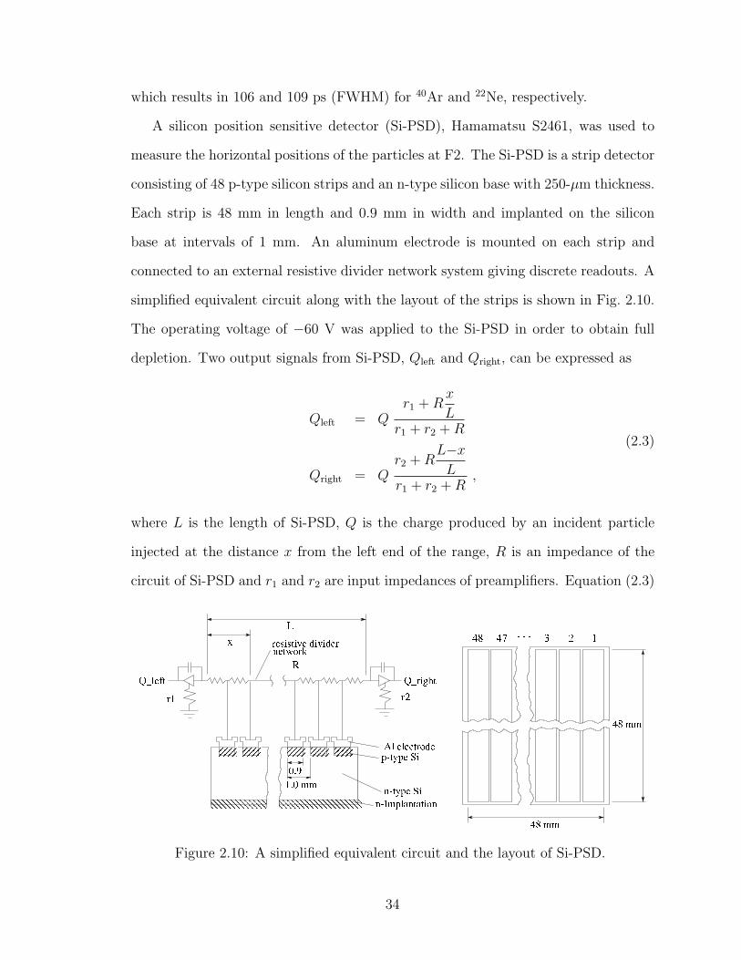
A silicon position sensitive detector (Si-PSD), Hamamatsu S2461, was used to

measure the horizontal positions of the particles at F2. The Si-PSD is a strip detector

consisting of 48 p-type silicon strips and an n-type silicon base with 250-µm thickness.

Each strip is 48 mm in length and 0.9 mm in width and implanted on the silicon

base at intervals of 1 mm. An aluminum electrode is mounted on each strip and

connected to an external resistive divider network system giving discrete readouts. A

simplified equivalent circuit along with the layout of the strips is shown in Fig. 2.10.

The operating voltage of −60 V was applied to the Si-PSD in order to obtain full

depletion. Two output signals from Si-PSD, Qleft and Qright, can be expressed as

Qleft = Qr1 + R

x

Lr1 + r2 + R

Qright = Qr2 + R

L−x

Lr1 + r2 + R

,

(2.3)

where L is the length of Si-PSD, Q is the charge produced by an incident particle

injected at the distance x from the left end of the range, R is an impedance of the

circuit of Si-PSD and r1 and r2 are input impedances of preamplifiers. Equation (2.3)

"!$#%& ' % )(+*

,& ' % )(+*,&.- % 0/ , /0*! ,

12 143 5 6 7

89$:"

";<*;<0*=)#$*=$*#$> , ?@! "A

BBB

C

D 7 D 6

EF

89$ "*G$H

IJ

IJ

Figure 2.10: A simplified equivalent circuit and the layout of Si-PSD.

34

can be written as

Qleft = Ax + B

Qright = A(L−x) + C .(2.4)

The parameters B and C are obtained by using a pulse generator and a dedicated

calibrator (See sec.3.4.). Then the position x is given by

x =Qleft −B

(Qleft−B) + (Qright−C)L . (2.5)

2.7 Data Acquisition

A schematic diagram of the data acquisition systems for the energy resolution mea-

surement and the longitudinal emittance measurements are shown in Figs. 2.11 and

2.12, respectively. In the case of the energy resolution measurement, data were stored

in HSM (CES High Speed Memory 8170) via FERA bus and FERA driver (LeCroy

4301). In the case of the longitudinal emittance measurements, on the other hand,

data were read via CAMAC at each event without buffering. In both cases, data

were stored and analyzed on a personal computer running a free-Unix clone, Linux.

Details of the data acquisition system can be found in Ref. [15].

2.7.1 Energy Resolution Measurement

The signal from HPGe detector was fed to a spectroscopy amplifier (ORTEC 671)

and formed to a Gaussian with shaping time of 6 µsec. The unipolar output (UNI in

Fig. 2.11) has a pulse height in proportion to the energy deposited in the HPGe. It

was digitized by an ORTEC AD413A analog-to-digital converter (ADC) with a 13-bit

resolution and subsequently fed to HSM to make energy spectra. The bipolar output

(BI) was used for monitoring signals. The logic signal output, counter & rate meter

35

TTL/NIM Delay TAC

756Logic Unit

G.GFI/FO

FI FI/FO

FERA4301

HSM OVFL

DRIVE

veto

stop

startveto

OUT____

Gate

CLR

Counting Room

stop

HSM

REQ BUSY

WAKWST

Ge SA

G.G

756Logic Unit

OutputRegister

G.G

CRMBI

UNI

(FI/FO)

Counting Room

Date Acquisition Softwarestart 1 stop 0

OVFL

DAQ ON

60 ns

Logic Delay 4303TFC

ActiveSlit

AMP CF8000

Counting Room

Counting Room startTAC

60 ns Delay

FERA

level 1 level 2

Scaler

4300B

AD413A

Figure 2.11: Data acquisition system for the energy resolution measurement.

Figure 2.12: Data acquisition system for the longitudinal emittance measurements.

36

(CRM), was fed to a logic unit (Phillips Scientific 756) and a gate generator (LeCroy

222) to make the gate for ADC. The signal from the active slit was amplified by 10,

discriminated by a constant-fraction discriminator (ORTEC CF8000) and fed to an

ORTEC 567 time-to-amplitude converter (TAC). The TAC output was converted by

AD413A and used for a veto.

2.7.2 Longitudinal Emittance Measurements

The signals from plastic scintillators, J1 and J2, were amplified by Phillips Scien-

tific 776 and fed to a constant fraction discriminator (CFD), Tennelec 454, in the

experimental area. The CFD outputs were transmitted to the counting room and

discriminated again by a discriminator (LeCroy 821). The outputs were subsequently

sent to a time-to-digital converter (TDC), KAIZU 3781A, in order to obtain the infor-

mation of particle arrival time. The outputs from the discriminator were also used to

make a coincidence signal between J1 and J2, which triggered the data acquisition.

The signals from J1 and J2 were also sent to an ADC (LeCroy 2449W). The Si-PSD

signals, Qleft and Qright, were transmitted to shaping amplifiers (ORTEC 671) via a

preamplifier and subsequently fed to an ADC (HOSHIN C008). It should be noted

that the RF signal fed to TDC represents the injection phase and is different from

the one fed to the RRC cavities, the phase of which is shifted by a phase shifter (Fig.

2.12).

37

Chapter 3

Analysis

3.1 Energy Calibration of HPGe

The output of HPGe was calibrated by using the standard γ-sources, 60Co, 22Na and

137Cs. Figure 3.1 shows the energy spectra for these sources. The background γ ray

from 40K, as seen in Fig. 3.1, was also used for calibration. The energies of gamma

rays and corresponding ADC channels are listed in Table 3.1. The regression line

obtained by the least squares method is

Energy [keV] = −4.03 + 0.923× ADC [channel] . (3.1)

The energy resolution at 1332.5-keV was 14.2 keV (FWHM) in this calibration. This

is reasonably good for measuring energies as large as ∼ 2 GeV, although the resolution

is generally 2 keV in ordinary γ-ray spectroscopies. The resolution at 1890 MeV is

expected to be

δE

E=

√1.333

1890

14.2

1332.5= 2.8×10−4

38

Figure 3.1: Energy spectra from 137Cs, 22Na and 60Co sources which are used for theenergy calibration of ADC channels. The peak from the background, 40K, was alsoobserved.

if estimated in the same manner as Sec. 1.3.2. The gain of spectroscopy amplifier for

the energy resolution measurement was determined to be 4.4 in such a way that 1890

MeV corresponded to 6000 channels, while the gain was 1500 in the γ-ray calibration.

39

Table 3.1: Energies of γ rays emitted by 60Co, 22Na, 137Cs and 40Kr, and the corre-sponding ADC channels.

ADC [channel] 558.4 721.1 1274.9 1385.5 1447.8 1587.8Energy [keV] 511.0 661.7 1173.3 1274.5 1332.5 1460.9

Source 22Na 137Cs 60Co 22Na 60Co 40K

40

Figure 3.2: Energy spectra for all events (unshaded) and for events without signalsfrom the active slit (shaded).

3.2 Veto by Active Slit

Figure 3.2 shows typical energy spectra detected by the HPGe at normal injection.

The unshaded one is the spectrum for all events without using the information from

the active slit. Two peaks are observed; one at higher energy is formed from particles

passing through the 1-mm aperture of active slit, while one at lower energy is from

particles which pass through the aperture of brass slit but not the active slit, thus lose

some energies in the 0.1-mm scintillator. The shaded one is the spectrum obtained by

rejecting events having signals from the active slit. It is clearly seen that the particles

penetrating the 0.1-mm scintillator are completely eliminated. The lower energy peak

in the unshaded spectrum has a slightly larger width than the one at higher energy,

due to the larger aperture of brass slit (3 mm) and the energy-loss straggling in the

scintillator, but the difference is not significant because the resolution of HPGe has

the largest contribution.

41

Figure 3.3: Typical time spectrum used for time calibration (upper panel). Pulsesfrom a time calibrator had a 10 ns interval over 100 ns range. The regression line isshown in the lower panel.

3.3 Time Calibration

The time calibration was performed by using pulses generated by a time calibrator

(ORTEC 462). Each of TDCs reading J1, J2 and RF signals was calibrated individ-

ually. Figure 3.3 shows one of typical time spectra for pulses having a 10 ns interval

over 100 ns range and the regression line obtained by the least squares method.

3.4 Position Calibration

Each of ADC channels of Si-PSD signals, Qleft and Qright, was calibrated by using a

pulse generator. One of typical spectra and a regression line obtained by the least

squares method are shown in Fig. 3.4. Then B and C in Eq. (2.5) were determined

42

Figure 3.4: Spectrum used for calibration of Left ADC (upper panel). The regressionline is shown in the lower panel.

in the following way. Equation (2.4) is reduced to

Qleft −B

x=

Qright − C

L− x, (3.2)

which is a straight line containing the point (B,C) in (Qleft, Qright) plot. Thus (B, C)

is given by the intersecting point of Qleft-Qright correlation lines for different x. These

correlation lines were obtained by using a pulse generator and a dedicated position

calibrator for Si-PSD. The result is shown in Fig. 3.5. However, Eq. (2.4) is correct

only in the ideal case. Since the real detector has stray capacitance, which makes

the time constant RC position-dependent, signals are not linear functions of x due to

the ballistic deficit in shaping circuits. In the present case, fortunately, the discrete

structure of the spectrum (Fig. 3.6) definitely gives us information on the absolute

position. A third order polynomial giving the correct position x was determined by

the least squares method. In the following analysis, random numbers in [0, 1] were

43

Figure 3.5: Qleft-Qright plot for different x generated by the dedicated position cali-brator. The inset is a closeup around the intersecting point.

added to x for removing spurious structure of the spectra.

3.5 Time of Flight Correction

The flight time of particle traveling from the RRC to the detector depends on the par-

ticle momentum. This effect must be corrected to obtain the longitudinal emittance

of the RRC. The time-of-flight (ToF) is given by

t =L

v=

LE

pc2,

where L is the flight path length, E is the total energy and p is the momentum of a

particle. The ToF difference δt is related to the momentum difference δp via

δt =

[L0

c2

∂

∂p

(E

p

)+

E0

p0c2

∂L

∂p

]δp

=

[− 1

γ20

+1

L0

∂L

∂p/p0

]t0

δp

p0

. (3.3)

44

Figure 3.6: Spectrum of x/L calculated by using Eq. (2.5) (upper panel). Discretepeaks reflecting the strip structure are clearly seen. The lower panel shows the regres-sion curve to deduce the correct position determined by the least squares method.

L0 is the length of the reference orbit. From the first quadrupole of QA02 (Fig. 2.4)

to SMART-F2, L0 = 89.5 m. The transfer matrix element∂L

∂p/p0

= (l|δ) can be esti-

mated, e.g., by using transport, where R56 = −(l|δ) . In the code cosy infinity

[16], even the correction coefficient ∂t/(∂T/T0) is directly given by −ME(5, 6) . While

the first term in Eq. (3.3) is independent of the transport condition, the second term

is very sensitive to the choice of transport parameters and changes even its sign easily.

It was determined for each case of 40Ar and 22Ne in the following way.

In the case of 40Ar beam, data were obtained displacing the phase of the RRC

Dee voltages relative to the injection phase in step of 2 (198 ps for 28.1-MHz RF).

Since the RF signal fed to TDC represents the injection phase (Sec. 2.7.2), the time

difference between the RF and the detector does not change if the acceleration is truly

isochronous, but it does change due to the phase compression described in Sec. 1.2.6.

45

According to Eq. (1.13), the shift by the phase compression is proportional to the

injection phase with respect to the RF, ∆φinj. (l|δ) has been artificially determined so

as to satisfy this relation. Figure 3.7 shows the time spectra corrected only by the first

term in Eq. (3.3). It is seen that time spectra at ∆φinj = +4 to −2 do not shift while

time spectra at ∆φinj = −4 and −6 do significantly. On the other hand, by assuming

(l|δ) = −35.5 cm/%, the corrected time spectra shift approximately in proportion to

their injection phases as shown in Fig. 3.8. This hypothetical value is consistent with a

transfer matrix element (l|δ) = −32.6 cm/% calculated by transport. Substituting

L0 = 89.5 m and γ0 = 1.1021 as well as (l|δ) = −35.5 cm/% into Eq. (3.3), ToF

correction is obtained as

δt = [−584.8−281.7]δp

p0

[ns] . (3.4)

In the case of 22Ne beam, the dependence of ToF on the particle momentum was

determined by slightly degrading the momentum with the charge stripper (Fig. 2.4).

The shift in (t, δ) plot directly gives the coefficient in Eq. (3.3). The used stripper was

a carbon foil with a thickness of 9 mg/cm2. Figure 3.9 shows the correlation spectra,

h2(t, δ) and h1(t, δ), detected at F2 with (right panel) and without the stripper (left

panel), respectively. The displacements, t0 and δ0, were determined so as to minimize

the chi squares defined by

χ2 =∑i, j

[ h1(ti, δj)− h2(ti−t0, δj−δ0) ]2 .

The obtained values are t0 = 0.525 ns and δ0 = −1.021× 10−3, resulting in the ToF

46

Figure 3.7: Time spectra with the first-term correction only. The injection phasewith respect to the RF phase of the RRC, ∆φinj, is displaced in step of 2.

Figure 3.8: Same as Fig. 3.7 but with the correction assuming (l|δ) = −35.5 cm/%.

correction to be

δt = −514.20δp

p0

[ns] . (3.5)

47

Figure 3.9: The correlation between the time and momentum of particles detected atF2 without the stripper (left) and with the stripper (right).

48

Figure 3.10: Beam spot on a ZnS scintillation target at the target position with (rightpanel) and without the stripper foil (left panel). Ticks on the target are marked in 5mm step.

To justify the above procedure, the beam spot on the target should not move

irrespective of the momentum, which is achieved by an achromatic transport. The

calculated transfer matrix from the stripper to the target is

x′

a′

y′

b′

l′

δ′

=

0.3620 0.1745 0 0 0 0.8351

−1.5762 2.0025 0 0 0 4.9694

0 0 0.4601 −0.0785 0 0

0 0 −1.1680 2.3725 0 0

−0.3115 0.0805 0 0 1 1.6120

0 0 0 0 0 1

x

a

y

b

l

δ

. (3.6)

(x|δ) is not zero but sufficiently small. It was experimentally verified by using a ZnS

scintillation target (Fig. 3.10).

49

Chapter 4

Results and Discussions

4.1 Energy Resolution of HPGe

Figure 4.1 shows typical energy spectra with the active slit at normal and 43 injec-

tions. The peak widths determined by a Gaussian peak fitting are 1.52 MeV and 1.80

MeV (FWHM), which correspond to relative energy spreads of δE/E = 8.0×10−4 and

9.5×10−4 for the normal and 43 injections, respectively. Subtracting the estimated

energy-loss straggling in the 300-µm Be window and the air between the exit vacuum

Figure 4.1: Energy spectra with the active slit at normal and 43 injections, respec-tively.

50

Table 4.1: Peak width in observed energy spectra, the contributions from energy-lossstraggling and the intrinsic energy resolution of HPGe at normal and 43 injectionsfor 1890-MeV 14N.

Injection Peak Straggling Beam Intrinsic UnitAngle Width Be Air Spread Resolution

Normal 1.52 0.72 0.24 0.47 1.23 MeV8.0 3.8 1.3 2.5 6.5 ×10−4

43 1.80 0.88 0.30 0.47 1.47 MeV9.5 4.7 1.6 2.5 7.7 ×10−4

(FWHM)

window and the Be window, the intrinsic energy resolution of HPGe becomes 1.23

MeV and 1.47 MeV (FWHM) for the normal and 43 injections, respectively. The

energy-loss straggling in the vacuum window and the light shield is negligibly small.

The results are summarized in Table 4.1.

Note that the present HPGe detector is not optimized for our purpose. For exam-

ple, the use of smaller Ge crystal decreases the leakage current and the capacitance,

which results in the lower electronics noise, and allows the use of small and thin Be

window, say 25 µm, resulting in the smaller energy-loss straggling. Since the intrinsic

resolution achieved in the present experiment is already at a level of practical use, it

is concluded that HPGe is promising as an energy detector for longitudinal emittance

measurements.

The energy resolution at 43 was slightly worse than that at normal injection,

contrary to our expectation that the inclined electric field with respect to the particle

path will improve the charge collection, leading to the improvement of energy reso-

lution. There are two possible reasons: One is that, because the HPGe detector was

not precisely set on the beam axis (Fig. 2.8), particles were injected near the edge

of crystal where the electric field can be weak. A weak electric field deteriorates the

charge collection and accordingly the energy resolution. The other is an underesti-

mation of energy-loss straggling in the Be window, which mainly contributes to the

51

systematic error of energy resolution. This is also suggested even from the data for

normal injection, as the observed resolution 6.5×10−4 is significantly worse than the

one expected from the γ-source data described in Sec. 3.1. The present estimation of

energy-loss straggling has some ambiguities since the data in this energy region are

rare. The error may be removed by directly measuring the energy-loss straggling in

a Be foil with the spectrometer.

4.2 Longitudinal Emittance of 40Ar Beam

— case of single turn extraction —

Figure 4.2 shows the longitudinal emittances of 3800-MeV 40Ar. δt is the extraction

time relative to the RF of the RRC, instead of the injection time, and is corrected

for ToF according to Eq. (3.4). The injection phase ∆φinj is displaced relative to

the RF of the RRC in step of 2 (198 ps for 28.1-MHz RF). Like in Fig. 1.7, it

is clearly seen that there is a quadratic correlation between δt and δT/T , which

is expected from Eq. (1.11). A sinusoidal curve corresponding to the RF of 28.1

MHz is displayed for eye-guide. The correlation is, however, smeared by fairly large

spread of distribution. The time and energy spreads are approximately 700 ps and

1.3×10−3 (FWHM), respectively. The energy resolution expected from (x|δ) of the

spectrometer, 2.5×10−4, can be deteriorated by several times due to the beam spread

on the target, ∼5 mm. The time resolution for the scintillators, on the other hand,

was confirmed to be 100 ps in the present experiment (Sec. 2.6.2). The other source

of time spread is not clear. It is unlikely that the beam in acceleration has such a

time spread. The investigation of this spread is critical for the longitudinal emittance

measurement. A smaller time spread will be particularly helpful to see the steep

correlations more clearly.

Figure 4.2 includes not only the sinusoidal correlation but also the effect of phase

52

Figure 4.2: Longitudinal emittances of 3800-MeV 40Ar. The injection phase ∆φinj isdisplaced relative to the RF of the RRC in step of 2.

53

compression discussed in Sec. 1.2.6 (upper panel in Fig. 4.3). The effect is directly

seen by taking the extraction time relative to the injection (middle panel in Fig. 4.3).

The projected spectra corresponding to the lower panel of Fig. 4.3 are presented in

Fig. 4.4. The shifts of spectra are deduced from Gaussian peak-fitting and plotted as

a function of ∆φinj in Fig. 4.5. According to Eq. (1.13), where Vext/Vinj = 1.6 for the

RRC, they are expected to lie on the solid line in Fig. 4.5. It is approximately the

case, but the deviation indicates a higher order effect, the origin of which is a future

problem.

54

Figure 4.3: Schematic illustration of phase compression effect for the case of narrow-bunched beam. The extraction time is either relative to the RF of the RRC (upperpanel) or relative to the injection (lower panel).

55

Figure 4.4: Projected spectra of the extraction time relative to the injection. Thephase of the RF with respect to the injection, ∆φinj, is shifted in step of 2.

56

Figure 4.5: Shifts of time spectra deduced from Fig. 4.4 plotted as a function of∆φinj. The solid line is a prediction from Eq. (1.13). The dashed curve is a thirdorder polynomial for eye-guide.

57

4.3 Longitudinal Emittance of 22Ne Beam

— case of multi-turn extraction —

The tuning of cyclotrons for the single-turn extraction is not always achieved at

RIKEN. In fact, it is sometimes the case that two or three turns are extracted for

experiments not requiring a high-quality beam, like ones using a secondary beam.

As a case of multi-turn extraction, the longitudinal emittance of 2420-MeV 22Ne is

discussed in this section.

The time structure of the extracted beam relative to the injection time is shown

in the upper panel of Fig. 4.6. Two peaks are observed separated by 33.2 ns, one of

which would disappear for the case of single-turn extraction. As described in Sec.

2.2, adjacent turns are extracted at different times from the main one by 33.2 ns

because hAVF/hRRC = 2/5 and frf = 30.10 and 15.05 MHz for the RRC and AVF,

respectively. Note that the main turn is extracted at an interval of 66.4 ns. The

longitudinal emittances for the main and adjacent turns are presented in the middle

panel of Fig. 4.6. There are two loci for the adjacent turn, suggesting a mixture of

two turns. Together with the main turn, all of the three turns have different δT -δt

correlations from each other. A possible explanation of this is illustrated in Fig. 4.7.

It is assumed that the beam is not injected at the phase of highest voltage and the

phase spread is relatively large. A part of the beam distribution is peeled off by the

extraction devices at the N−1 turn, the main part at the N turn and the remaining at

the N+1 turn. They are extracted at different phases and accordingly with different

δT -δt correlations. This idea is supported by the data obtained with the lower Dee

voltage by 2×10−3 relative to the nominal value. They are shown in the lower panel

of Fig. 4.6. Here the beam in the N−1 turn is not extracted and a smaller part of the

beam is extracted in the main turn, as expected from the lower panel of Fig. 4.7. This

illustration, however, does not explain the data quantitatively and a further study

58

Figure 4.6: Time spectrum (upper panel), the longitudinal emittances for the mainand adjacent turns at the nominal Dee voltage (middle panels) and at a slightlylowered Dee voltage (lower panels). Straight lines are for eye-guide.

59

Figure 4.7: Schematic illustration of δT -δt correlations for neighboring turns at thenominal Dee voltage (upper panel) and at a slightly lowered Dee voltage (lower panel).

60

must be made.

61

Chapter 5

Conclusions

It is important to measure the longitudinal emittance of the beam coming from the

RRC for successful operations of the new facility, RIBF. A compact and convenient

energy detector is desired for routine operations, thus the use of a HPGe detector

was proposed and the feasibility of its use with energetic heavy ions was studied. The

energy resolution of a HPGe detector for a high-energy heavy ion, 135-MeV/A 14N,

has been measured using a magnetic spectrometer for defining the particle energies.

A reasonably good resolution, δE/E = 6.5×10−4 (FWHM), has been observed by

a HPGe detector with the crystal size as large as φ70 mm in diameter and 30 mm

in thickness. As a better resolution is expected for smaller crystals, the HPGe is

promising as an energy detector for longitudinal emittance measurements.

Using the same magnetic spectrometer, the longitudinal emittances have been

measured for the 3800-MeV 40Ar beam, as a case of the single-turn extraction, and

for the 2420-MeV 22Ne beam, as a case of the multi-turn extraction. For the 40Ar

beam, by displacing the RF phase of the RRC from −6 to +4 in step of 2, a

quadratic correlation reflecting the sinusoidal RF voltage as well as the effect of

phase compression have been observed. The time spread, however, was larger than

expected from the detector resolution and acceleration mechanism. Its origin should

62

be investigated to observe the correlation more clearly. For the 22Ne beam, it was

found from the time structure of the beam that several turns were extracted. Besides,

the longitudinal emittance had a structure suggesting a mixture of different turns.

An illustrative explanation has been proposed for identifying each turn. Data with a

different Dee voltage are consistent with this idea. However, a further study must be

made to obtain a quantitative understanding.

In conclusion, it has been demonstrated that the measurement of longitudinal

emittance provides rich information on the acceleration condition and will be very

helpful for the beam tuning of the present and new facilities.

63

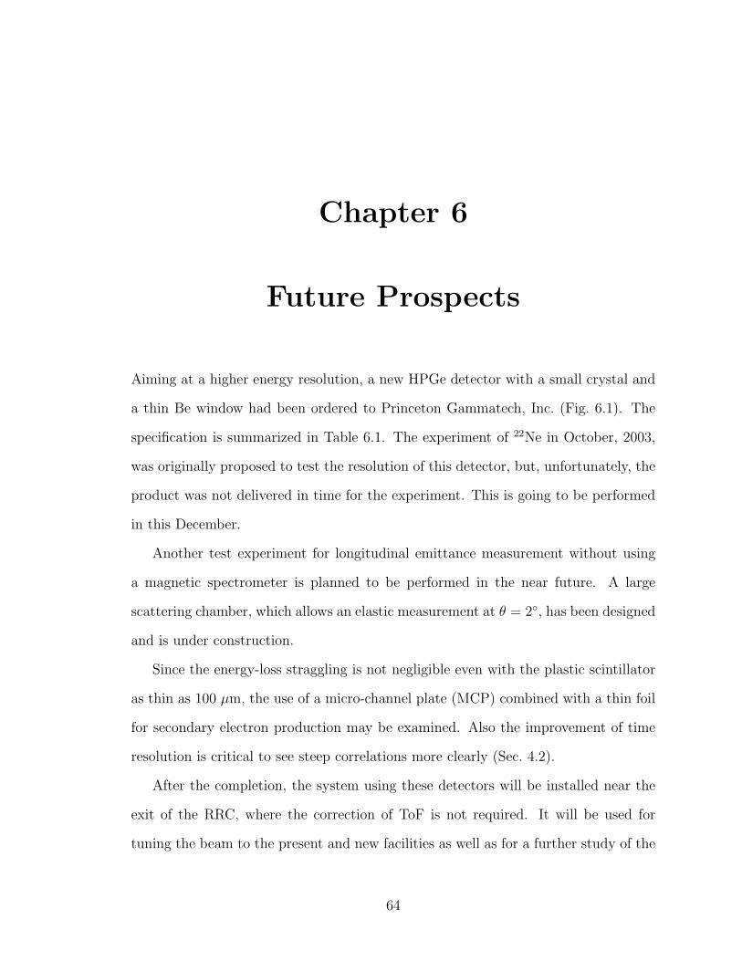
Chapter 6

Future Prospects

Aiming at a higher energy resolution, a new HPGe detector with a small crystal and

a thin Be window had been ordered to Princeton Gammatech, Inc. (Fig. 6.1). The

specification is summarized in Table 6.1. The experiment of 22Ne in October, 2003,

was originally proposed to test the resolution of this detector, but, unfortunately, the

product was not delivered in time for the experiment. This is going to be performed

in this December.

Another test experiment for longitudinal emittance measurement without using

a magnetic spectrometer is planned to be performed in the near future. A large

scattering chamber, which allows an elastic measurement at θ = 2, has been designed

and is under construction.

Since the energy-loss straggling is not negligible even with the plastic scintillator

as thin as 100 µm, the use of a micro-channel plate (MCP) combined with a thin foil

for secondary electron production may be examined. Also the improvement of time

resolution is critical to see steep correlations more clearly (Sec. 4.2).

After the completion, the system using these detectors will be installed near the

exit of the RRC, where the correction of ToF is not required. It will be used for

tuning the beam to the present and new facilities as well as for a further study of the

64

Table 6.1: Specifications of Ge detector (Princeton Gammatech: IGP1010185 Model).

Crystal Diameter Thickness Be End CapType Window Length

Planar Ge φ10 mm 10 mm 50.8 µm 200 mm

Preamplifier Gain Energy Vacuum DewarType Range Flange Volume

Resistive Feedback 1/60 ' 2 GeV CF φ70 mm 7.5 `

Figure 6.1: Overview of the newly fabricated HPGe detector.

65

beam from the RRC. Particularly important for the operation of the new facility is a

study of 60-MeV/A beams, which are obtained by using the LINAC as the injector,

instead of the AVF cyclotron, but were not available in the present experiments.

66

Appendix A

Angular Distribution of Elastic

Scattering

The knowledge on the elastic scattering cross section is important for designing ex-

periments without using a magnetic spectrometer, but data for heavy ions are scarce.

The angular distribution of elastic scattering of 14N on 197Au target at E/A = 135

MeV/A has been obtained in the present experiment. The result of the cross section

in the laboratory frame is presented in Fig. A.1. It is remarkable that the cross section

varies exponentially and the distribution is much steeper than that of the Coulomb

scattering from a point charge (Rutherford scattering). Since the cross section be-

comes very small at backward angles, it will be appropriate to make measurements

at θ = 2–3 in this energy region. The counting rate dY/dt is related to the cross

section dσ/dΩlab by

dY

dt= In

dσ

dΩlab

∆Ωlab , (A.1)

where I denotes the beam intensity, n the thickness of target and ∆Ωlab the detector

solid angle.

67

2 3 4 5 6

10−1

100

101

102

expRuth

θlab (deg)

dσ/dΩ(b/sr)

197Au(14N,14N)197Au elasticE=135 MeV/u

Figure A.1: Angular distribution of 197Au(14N,14 N)197Au elastic scattering at E/A =135 MeV/A compared with Rutherford scattering. The exponential line is for eye-guide.

68

Acknowledgement

First of all, I would like to express my appreciation to Prof. Martin Berz for preparing

the fascinating course of VUBeam and for his continuous support during my study.

I am deeply indebted to Dr. Akira Goto, the chief of Beam Dynamics Division at

RIKEN Accelerator Research Facility, for providing me an opportunity to make this

study. I am grateful to Prof. Toshio Kobayashi at Tohoku University who kindly

loaned us the HPGe detector, allowed us to modify the preamplifier and participated

in the experiment. Also my thanks go to Prof. Hiroyuki Okamura at Saitama Univer-

sity (presently at Tohoku University) who has been sincerely concerned about me and

gave me countless pieces of advice and comment in the course of the experiment, data

analysis and writing of this thesis. Theoretical discussions on the experimental results

with Dr. Nobuhisa Fukunishi are gratefully acknowledged. I sincerely appreciate the

help from Dr. Naruhiko Sakamoto, who provided me a supportive environment for

learning about accelerator concepts and made my life at RIKEN delightful. I would

like to thank Dr. Hiromichi Ryuto for his support in the experiments and for his

careful reading of my thesis. I am thankful to Dr. Kimiko Sekiguchi-Sakaguchi who

participated in the experiments and always cheered me heartily. I wish to express

my gratitude to all the staff members of the RIKEN Accelerator Research Facility,

particularly to the RIKEN cyclotron crew for their excellent machine operation, to

Dr. Yasushige Yano, the director of the RIKEN Accelerator Research Facility, who

generously accepted me for making a study at RIKEN, and to Dr. Masayuki Kase

69

for his arrangement of the experiments. I am grateful to Prof. Harry Weerts for his

serving my defense committee and for his perceptive comments on my thesis. I am

much obliged to Prof. Kyoko Makino for her cordial advice through the course of the

study and for her serving my defense committee. Last but not least, I would like to

thank my family with my whole heart for their encouragement.

70

BIBLIOGRAPHY

[1] H. Wiedemann, Particle Accelerator Physics I & II, second edition, Springer-Verlag, 1998.

[2] Mario Conte and William W MacKay, AN INTRODUCTION TO THE PHYSICSOF PARTICLE ACCELERATORS, first edition, World Scientific Publishing Co.Pte. Ltd, 1991.

[3] J. I. M. Botman and H. L. Hadedoorn, EXTRACTION FROM CYCLOTRONS,report CERN 96-02 article/p169

[4] B. Martin, R. C. Sethi and K. Ziegler, Measurements and Studies of the Longitu-dinal Phase Space at VICKSI, unpublished.

[5] V. S. Pandit, Characteristics of the cyclotron beam in the longitudinal phase space,Nucl. Instr. and Meth. A 414 (1998) 127.

[6] R. W. Muller and R. W. Mahrt, Phase compression and phase dilatation in theisochronous cyclotron, Nucl. Instr. and Meth. 86 (1970) 241.

[7] W. Joho, Application of the phase compression-phase expansion effect forisochronous storage rings, Particle Accelerators, 6 (1974) 41.

[8] W. R. Leo, Techniques for Nuclear and Particle Physics Experiments, secondedition, Springer-Verlag, 1994.

[9] G. F. Knoll, Radiation Detection and Measurement, third edition, John Willy &Sons, 2000.

[10] D. L. Friesel, B. S. Flanders and R. H. Pehl, A variable geometry high-puritygermanium detector telescope system for use with intermediate energy chargedparticles, Nucl. Instr. and Meth., 207 (1983) 403.

[11] M. Kurokawa et al., Radiation Damage Factor for Ion-Implanted Silicon Detec-tors Irradiated with Heavy Ions, IEEE Trans. Nucl. Sci., 42 (1995) 163.

[12] T. Ichihara et al., Spin-Isospin Resonances Observed in the (d, 2He) and(12C, 12N) Reactions at E/A = 135 MeV, Nucl. Phys. A569 (1994) 287c.

71

[13] A. Goto et al., Beam test and operation of the flattop acceleration system in theRIKEN AVF cyclotron, RIKEN Accel. Prog. Rep. 36 (2003) 287.

[14] D. C. Carey, K. L. Brown and F. Rothacker, Third-Order TRANSPORT withMAD Input, A Computer Program for Designing Charged Particle Beam Trans-port Systems, FERMILAB-Pub-98/310, SLAC-R-530 and UC-414.

[15] H. Okamura, Fast data acquisition system for the spectrometer SMART atRIKEN, Nucl. Instr. and Meth., A 443 (2000) 194.

[16] M. Berz and J. Hoefkens, COSY INFINITY Version 8.1 Programming Manual,Technical Report MSUCL-1196 (2001), National Superconducting Cyclotron Lab-oratory, Michigan State University; K. Makino and M. Berz, COSY INFINITYversion 8, Nucl. Instr. and Meth. A 427 (1999) 338.

72