development of precise gps/ins/wheel speed … ntm 2006, 18-20 january 2006, monterey, ca 1...

ION NTM 2006, 18-20 January 2006, Monterey, CA 1

Development of Precise GPS/INS/Wheel Speed Sensor/Yaw Rate Sensor Integrated Vehicular

Positioning System

J. Gao, M.G. Petovello and M.E. Cannon Position, Location And Navigation (PLAN) Group

Department of Geomatics Engineering Schulich School of Engineering

University of Calgary BIOGRAPHY Jianchen Gao is a PhD candidate in the Department of Geomatics Engineering at the University of Calgary. He received a PhD degree in Mechatronics at the Beijing Institute of Technology, an MSc in Automatic Control at the Beijing Institute of Technology and a BSc in Automatic Control at the Hebei University of Science and Technology. His current research area is in GPS/INS/On-board vehicle sensor integrated positioning and navigation systems. Dr. Mark Petovello holds a PhD from the Department of Geomatics Engineering at the University of Calgary where he is a senior research engineer in the Position, Location And Navigation (PLAN) group. He has been involved in various navigation research areas since 1998, including satellite-based navigation, inertial navigation, reliability analysis, and dead-reckoning sensor integration. Dr. M. Elizabeth Cannon is Professor and Head of Geomatics Engineering at the University of Calgary. She has been involved in GPS research and development since1984, and has worked extensively on the integration of GPS and inertial navigation systems for precise aircraft positioning. Dr. Cannon is a Past President of the ION and is currently Chair of the Satellite Division. ABSTRACT This paper aims to develop a more precise vehicular positioning system during GPS outages by integrating GPS, a tactical grade HG1700 IMU, as well as Wheel Speed Sensor and a Yaw Rate Sensor. Using a tight coupling strategy, three types of sensor integration schemes are proposed, namely GPS/INS/Wheel Speed Sensor, GPS/INS/Yaw Rate Sensor and GPS/INS/Yaw Rate Sensor/Wheel Speed Sensor. The models for each of

the schemes are discussed in detail including the sensor error models. The benefits after integrating the Wheel Speed Sensor and the Yaw Rate Sensor are investigated in terms of positioning accuracy during GPS data outages. Furthermore, the reduction in the time to fix the carrier phase ambiguities after various GPS outage durations is analyzed. INTRODUCTION To meet the requirements for vehicle safety and stability control such as forward-collision avoidance, significant attention has been paid to new sensor systems in recent years. Among them are anti-lock brake systems (ABS), traction control (TC), and vehicle stability control systems (VSC) which have already found their way into production passenger vehicles (Tseng et al., 1999). In most autonomous vehicle control and vehicle stability control systems, GPS and other dead-reckoning sensors are being employed to provide navigation and positioning information (Bevly, 1999). With respect to GPS, centimeter-level accuracies can be achieved by using carrier phase measurements in a double difference approach whereby the integer ambiguities are resolved correctly. However, difficulties arise during significant shading from obstacles such as buildings, overpasses and trees. This has led to the development of integrated systems whereby GPS is complemented by an inertial navigation system (INS). In such a system, GPS provides long-term, accurate and absolute positioning information which is subject to the blockage of line-of-sight signals as well as signal interference or jamming. Additionally, its measurement update rate is relatively low (typically less than 20 Hz). By contrast, an INS is autonomous and non-jammable, and most IMU data rates exceed 50 Hz with some reaching into several hundreds of Hertz. However, the weak points of INS are that its


navigation quality degrades with time, and its accuracy depends on the quality of INS sensors. GPS/INS integrated systems have been studied extensively. Based on the concept of lower cost and high accuracy, Petovello (2003) integrated carrier phase DGPS and a tactical grade IMU to provide decimeter-level accuracies during GPS outages. By integrating GPS and low cost inertial sensors, Sukkarieh (2000) developed a low cost, high integrity, aided inertial navigation system for use in autonomous land vehicle applications. Positioning accuracy and system redundancy have crucial impacts on the performance and reliability of autonomous vehicle control systems and vehicle safety and stability control systems. The more accurate the positioning system, the more reliable the vehicle autonomy or the safety control. The importance of sensor redundancy lies in the fact that any sensor failure due to mechanical, electrical or an external disturbance could lead to a disastrous result if the failed sensor was the only sensor on-board (Redmill, 2001). To improve accuracy and redundancy, significant work has also been done to integrate GPS with other lower cost dead-reckoning sensors to aid positioning and/or attitude determination. These sensors have ranged from the use of a compass, tilt meter and fiber-optic gyro for vehicle pitch and azimuth estimation (Harvey, 1998), to the integration of GPS with an on-board ABS, odometer and gyro for positioning in urban areas (Stephen, 2000). Wheel Speed Sensors are fundamental components of an ABS which is standard equipment on nearly all vehicles (Hay, 2005). Kubo et al. (1999) implemented a GPS/INS/Wheel Speed Sensor integrated system in the wander angle frame for land-vehicle positioning, and proposed an algorithm to calibrate the two tilt angles (azimuth angle and pitch angle) between the Wheel Speed Sensor and the IMU body frame. Based on the above discussion, with particular emphasis on Petovello (2003), this research aims to develop a more precise vehicular positioning system during GPS outages by integrating GPS, a tactical grade HG1700 IMU, as well as Wheel Speed Sensors and a Yaw Rate Sensor from a vehicle stability control (VSC) system. The research focuses on how to integrate the Wheel Speed and Yaw Rate Sensors with GPS/INS in an effective way and what benefits can be gained through this approach. The accuracy required is at the centimeter-level so carrier phase GPS measurements will be used. To be precise, an on-line calibration algorithm was designed to estimate the three tilt angles between the vehicle frame and the IMU body frame using an extended Kalman filter. Non-holonomic constraints are also considered for the GPS/INS/Wheel Speed Sensor integration strategy. Furthermore, the scale factor of the Wheel Speed Sensor and the bias of the Yaw Rate Sensor are augmented to the

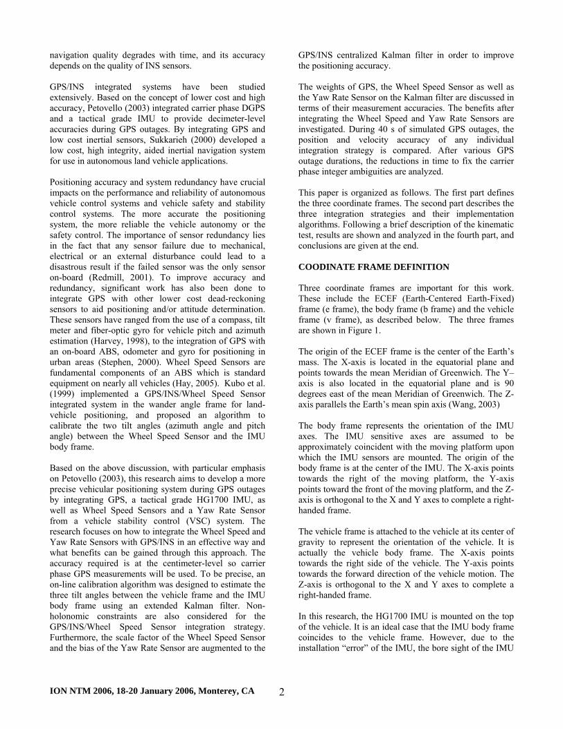
GPS/INS centralized Kalman filter in order to improve the positioning accuracy. The weights of GPS, the Wheel Speed Sensor as well as the Yaw Rate Sensor on the Kalman filter are discussed in terms of their measurement accuracies. The benefits after integrating the Wheel Speed and Yaw Rate Sensors are investigated. During 40 s of simulated GPS outages, the position and velocity accuracy of any individual integration strategy is compared. After various GPS outage durations, the reductions in time to fix the carrier phase integer ambiguities are analyzed. This paper is organized as follows. The first part defines the three coordinate frames. The second part describes the three integration strategies and their implementation algorithms. Following a brief description of the kinematic test, results are shown and analyzed in the fourth part, and conclusions are given at the end. COODINATE FRAME DEFINITION Three coordinate frames are important for this work. These include the ECEF (Earth-Centered Earth-Fixed) frame (e frame), the body frame (b frame) and the vehicle frame (v frame), as described below. The three frames are shown in Figure 1. The origin of the ECEF frame is the center of the Earth’s mass. The X-axis is located in the equatorial plane and points towards the mean Meridian of Greenwich. The Y–axis is also located in the equatorial plane and is 90 degrees east of the mean Meridian of Greenwich. The Z-axis parallels the Earth’s mean spin axis (Wang, 2003) The body frame represents the orientation of the IMU axes. The IMU sensitive axes are assumed to be approximately coincident with the moving platform upon which the IMU sensors are mounted. The origin of the body frame is at the center of the IMU. The X-axis points towards the right of the moving platform, the Y-axis points toward the front of the moving platform, and the Z-axis is orthogonal to the X and Y axes to complete a right-handed frame. The vehicle frame is attached to the vehicle at its center of gravity to represent the orientation of the vehicle. It is actually the vehicle body frame. The X-axis points towards the right side of the vehicle. The Y-axis points towards the forward direction of the vehicle motion. The Z-axis is orthogonal to the X and Y axes to complete a right-handed frame. In this research, the HG1700 IMU is mounted on the top of the vehicle. It is an ideal case that the IMU body frame coincides to the vehicle frame. However, due to the installation “error” of the IMU, the bore sight of the IMU


is misaligned with the vehicle frame in most cases. It is therefore necessary to calibrate the tilt angles between the body frame and the vehicle frame in the integrated algorithms.

Figure 1 Coordinate Frame Definition

INTEGRATION STRATEGIES & ALGORITHMS Using a tight coupling strategy, three types of integration strategies which are mechanized in the ECEF frame are proposed by integrating GPS, the INS as well as several on-board vehicle sensors including Wheel Speed Sensors and an automotive grade Yaw Rate Sensor. These include: • GPS/INS/Wheel Speed Sensor (GPS/INS/WSS); • GPS/INS/Yaw Rate Sensor (GPS/INS/YRS) , and; • GPS/INS/Yaw Rate Sensor/Wheel Speed Sensor

(GPS/INS/YRS/WSS). Tight coupling strategy combines all available sensor measurements at each epoch to obtain a globally optimal solution using one centralized Kalman filter.

For the equipment used, the IMU data rate is 100 Hz, and its mechanization equation output rate is set to 20 Hz. The IMU mechanization equations were implemented in the

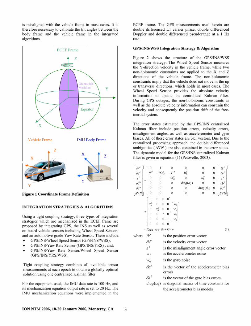
ECEF frame. The GPS measurements used herein are double differenced L1 carrier phase, double differenced Doppler and double differenced pseudorange at a 1 Hz rate. GPS/INS/WSS Integration Strategy & Algorithm Figure 2 shows the structure of the GPS/INS/WSS integration strategy. The Wheel Speed Sensor measures the Y-direction velocity in the vehicle frame, while two non-holonomic constraints are applied to the X and Z directions of the vehicle frame. The non-holonomic constraints imply that the vehicle does not move in the up or transverse directions, which holds in most cases. The Wheel Speed Sensor provides the absolute velocity information to update the centralized Kalman filter. During GPS outages, the non-holonomic constraints as well as the absolute velocity information can constrain the velocity and consequently the position drift of the free-inertial system. The error states estimated by the GPS/INS centralized Kalman filter include position errors, velocity errors, misalignment angles, as well as accelerometer and gyro biases. All of these error states are 3x1 vectors. Due to the centralized processing approach, the double differenced ambiguities ( N∇∆ ) are also contained in the error states. The dynamic model for the GPS/INS centralized Kalman filter is given in equation (1) (Petovello, 2003).

(1)

0000I0000000000000000

0000000)(000000)(000000000200000

/

f

wGxF

wwww

IR

R

Ndb

vr

diagdiag

RRFN

I

Ndb

vr

INSGPS

d

b

web

eb

b

b

e

e

e

i

i

eb

eie

eb

eeie

e

b

b

e

e

e

⋅+⋅=

⎥⎥⎥⎥

⎦

⎤

⎢⎢⎢⎢

⎣

⎡

⋅

⎥⎥⎥⎥⎥⎥⎥⎥

⎦

⎤

⎢⎢⎢⎢⎢⎢⎢⎢

⎣

⎡

+

⎥⎥⎥⎥⎥⎥⎥⎥

⎦

⎤

⎢⎢⎢⎢⎢⎢⎢⎢

⎣

⎡

∇∆

⋅

⎥⎥⎥⎥⎥⎥⎥⎥

⎦

⎤

⎢⎢⎢⎢⎢⎢⎢⎢

⎣

⎡

−−

Ω−−Ω−

=

⎥⎥⎥⎥⎥⎥⎥⎥

⎦

⎤

⎢⎢⎢⎢⎢⎢⎢⎢

⎣

⎡

∇∆

δ

δδεδδ

βα

δδεδδ

&

&

&&

&

&

where erδ is the position error vector

evδ is the velocity error vector

eε is the misalignment angle error vector

fw is the accelerometer noise

ww is the gyro noise

bbδ is the vector of the accelerometer bias

errors

bdδ is the vector of the gyro bias errors

)( idiag α is diagonal matrix of time constants for the accelerometer bias models

X

Y

Equator

Z

ECEF Frame

Y

Vehicle Frame IMU Body Frame

Z

Y

X Z

X

Greenwich Meridian

ION

)( idiag β is diagonal matrix of time constants for the gyro bias models

bw is the driving noise for the accelerometer biases

dw is the driving noise for the gyro biases

ebR is the direction cosine matrix between b

frame and e frame xδ is the error states vector, and

INSGPSF / is the dynamic matrix for GPS/INS integration strategy

As implied by the above model, the bias states are modeled as first-order Gauss-Markov processes.

Figu

In practical use, the tire radius is subject to a change of the load and the driving conditions. Additionally, the IMU body frame does not always coincide with the vehicle frame. Thus, the scale factor of the Wheel Speed Sensor and the tilt angles between the vehicle and body frames are augmented into the error states of GPS/INS centralized Kalman filter. The dynamic model in equation (1) is accordingly changed to equation (2) below. The Wheel Speed Sensor scale factor and the tilt angles between the b and v frames are modeled as random constants.

b

vr

F

b

vr

b

e

e

e

INSGPSb

e

e

e

⎥⎥⎥⎥⎥⎤

⎢⎢⎢⎢⎢⎡

⋅⎥⎥⎥⎥⎥⎤

⎢⎢⎢⎢⎢⎡

=⎥⎥⎥⎥⎥⎤

⎢⎢⎢⎢⎢⎡

00|00|00|00|

/

δεδδ

δεδδ

&

&

&

&

K

z 20 Hz

• G• A

G

M

100 H

NTM 2006, 18-20 January 2006, Mon

re 2 GPS/INS/WSS Integration Strate

Nd

Nd bb

⎥⎥⎥

⎢⎢⎢∇∆⎥

⎥⎥

⎢⎢⎢

−−−−−−−−⎥⎥⎥

⎢⎢⎢

∇∆00| δδ

&&

Mechanization Integration

+

• Wheel Speed Sensor • Non-holonomic constraints

1 Hz Vδ

δGPS

alman filter

-

GPS measurements • DD L1 carrier phase • DD Doppler • DD pseudorange

yros ccelerometers

PS update WSS update

Position (3) Velocity (3)

Misalignment angles (Gyro biases (3)

Accelerometer biases GPS ambiguities

WSS scale factor (1B to V frame tilt angles

KaF

eas Res

Position VelocityAttitude

wGF

wwww

II

RR

SS

WSSINSGPS

d

b

w

eb

eb

vbvb

⋅+⋅=

⎥⎥⎥⎥

⎦

⎤

⎢⎢⎢⎢

⎣

⎡

⋅

⎥⎥⎥⎥⎥⎥⎥⎥⎥⎥⎥

⎦

⎤

⎢⎢⎢⎢⎢⎢⎢⎢⎢⎢⎢

⎣

⎡

+

⎥⎥

⎦⎢⎢

⎣⎥⎥⎥

⎦⎢⎢⎢

⎣⎥⎥⎥

⎦⎢⎢⎢

⎣ −−

x

(2)

000000000000

0000000000000000

00|0000000|00000

//

f

δ

εδ

εδ&

&

where WSSINSGPSF // is the dynamic matrix for GPS/INS/WSS integration strategy, Sδ is the Wheel Speed Sensor scale factor error state, and

[ ]Tvb δγδβδαε =− is the error vector of the tilt angles between the body frame and the vehicle frame

3)

(3)

) (3)

Velocity in vehicle frame

corresponding to the X, Y and Z axes respectively. Since the wheel speed is measured in the vehicle frame, and the velocities in GPS/INS system are parameterized in ECEF frame, the WSS update can be either carried out in the e frame by transforming the WSS measurement into the e frame or carried out in the v frame by transforming the GPS/INS integrated velocities into the v frame. In this research, the WSS update is carried out in v frame, and the GPS/INS integrated velocities are transformed from e frame into v frame. The measurement equation is expressed in equation (3) with two non-holonomic constraints being applied into the X and Z axes of the

Estimated satellite measurement

-

vehicle frame.
IMU data flow
+

Error states
Centralized KF
lman ilter urementiduals

terey, CA 4

gy

( ) eTeb

vbWSS vRRvS ⋅⋅=

⎥⎥⎥

⎦

⎤

⎢⎢⎢

⎣

⎡⋅0

0 (3)


where WSSv is the Wheel Speed Sensor measurement, S

is the Wheel Speed Sensor scale factor, and vbR is the

direction cosine matrix between the b and v frames calculated by the following:

( ) ( ) ( )βαγ 213 RRRRvb ⋅⋅= (4)

where γβα ,, are the tilt angles between the b and v frames with respect to the X, Y and Z axes, respectively. The measurement model in the extended Kalman filter is generally expressed by equation (5):

mxHZ ωδ +⋅= (5)

where H is the design matrix, mω is the measurement noise and Z is the measurement residual. By linearizing equation (3), the measurement residual is expressed as in equation (6)

( ) vWSS

eTeb

vbWSS vvSvRRvSZ −

⎥⎥⎥

⎦

⎤

⎢⎢⎢

⎣

⎡⋅=⋅⋅−

⎥⎥⎥

⎦

⎤

⎢⎢⎢

⎣

⎡⋅=

0

0

0

0

(6)

where vv is the integrated velocity expressed in the v frame. The design matrix is expressed by a matrix in equation (7).

( ) ( )⎥⎥⎦

⎤

⎢⎢⎣

⎡

−⋅⋅⋅=

××

××V

WSS

ETeb

vb

Teb

vb

VvOOOVRRRROH

ARAR33

3333 .... (7)

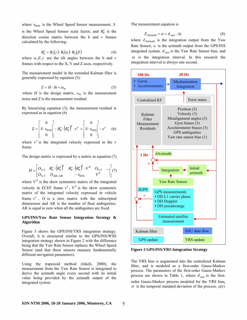
where EV is the skew symmetric matrix of the integrated velocity in ECEF frame ev , VV is the skew symmetric matrix of the integrated velocity expressed in vehicle frame vv , O is a zero matrix with the subscripted dimensions and AR is the number of float ambiguities. AR is equal to zero when all the ambiguities are fixed. GPS/INS/Yaw Rate Sensor Integration Strategy & Algorithm Figure 3 shows the GPS/INS/YRS integration strategy. Overall, it is structured similar to the GPS/INS/WSS integration strategy shown in Figure 2 with the difference being that the Yaw Rate Sensor replaces the Wheel Speed Sensor (and that these sensors measure fundamentally different navigation parameters). Using the trapezoid method (Jekeli, 2000), the measurement from the Yaw Rate Sensor is integrated to derive the azimuth angle every second with its initial value being provided by the azimuth output of the integrated system.

The measurement equation is

tdZ yawAzimuth ∆⋅+= α (8) where AzimuthZ is the integration output from the Yaw Rate Sensor, α is the azimuth output from the GPS/INS integrated system, yawd is the Yaw Rate Sensor bias, and

t∆ is the integration interval. In this research the integration interval is always one second.

Figure 3 GPS/INS/YRS Integratio

The YRS bias is augmented into tfilter, and is modeled as a firsprocess. The parameters of the firsprocess are shown in Table 1, worder Gauss-Markov process modeσ is the temporal standard deviatio


δAzimuth

+

Kalman Filter

MeasurementResiduals

Centralized KF

Estimated satellitemeasurement

Integration

δGPS+

-

100 Hz • Gyros • Accelerometers

GPS measurements • DD L1 carrier phas• DD Doppler • DD pseudorange

Error states

Position (3) Velocity (3)

Misalignment angles (3) Gyro biases (3)

Accelerometer biases (3) GPS ambiguities

Yaw rate sensor bias (1)

1 Hz

r

e

IM

z

Yaw Rate Sensor

Initial azimuth

e

U data flow
Kalman filte
GPS updat

20 H

YRS update

-

n Strategy

he centralized Kalman t-order Gauss-Markov t-order Gauss-Markov here yawd is the first-led for the YRS bias, n of the process, )(tu


is a unity white noise sequence that drives the system, and Yawβ is the inverse of the process time constant.

Table 1 First-Order Gauss Markov Process Parameters for Yaw Rate Sensor Bias

deg/s 059.0=σ First-order Gauss-Markov process ( )tudd YawYawYawYaw ⋅+⋅−= βσβ 22& h 75.01 =Yawβ

Equation (9) shows the dynamic model by augmenting the Yaw Rate Sensor bias.

(9)

1000000000000000000000000000000

|000000|

0|0|0|0|0|0|

/

⎥⎥⎥⎥⎥⎥

⎦

⎤

⎢⎢⎢⎢⎢⎢

⎣

⎡

⎥⎥⎥⎥⎥⎥⎥⎥⎥

⎦

⎤

⎢⎢⎢⎢⎢⎢⎢⎢⎢

⎣

⎡

+

⎥⎥⎥⎥⎥⎥⎥⎥⎥

⎦

⎤

⎢⎢⎢⎢⎢⎢⎢⎢⎢

⎣

⎡

∇∆

⋅

⎥⎥⎥⎥⎥⎥⎥⎥⎥⎥⎥

⎦

⎤

⎢⎢⎢⎢⎢⎢⎢⎢⎢⎢⎢

⎣

⎡

−−−−−−−−

=

⎥⎥⎥⎥⎥⎥⎥⎥⎥

⎦

⎤

⎢⎢⎢⎢⎢⎢⎢⎢⎢

⎣

⎡

∇∆

yaw

d

b

w

feb

eb

yawYaw

INSGPS

yaw

wwwww

II

RR

dNdb

vr

F

d

Ndb

vr

δ

δδεδδ

βδ

δδεδδ

&

&&

&&

&

&

where yawdδ is the error state of the Yaw Rate Sensor bias,

Yawβ is the inverse of the time constant, and yawω is the driving noise of the Yaw Rate Sensor bias. The design matrix is a matrix expressed in equation (10), which is derived from the measurement equation (8).

⎥⎥⎦

⎤

⎢⎢⎣

⎡

∆=

×××

××

tOOOROOH

ARAR

le

3333

row 3rd3333 ...)( (10)

where leR is the direction cosine matrix between the e

frame and the local level frame. Since the estimated error states are defined in ECEF frame, and the azimuth angle is related to the local level frame, the third row in the l

eR matrix appears in the design matrix. In this integration strategy, the Yaw Rate Sensor provides the azimuth update to the centralized filter. Since only the relative azimuth is computed from the Yaw Rate Sensor, the performance of this integration strategy has a close relationship with the measurement accuracy of the Yaw Rate Sensor. Given the low quality Yaw Rate Sensor, it is difficult to estimate both the azimuth and the YRS bias. As such, the benefit in terms of azimuth accuracy is expected to be somewhat limited.

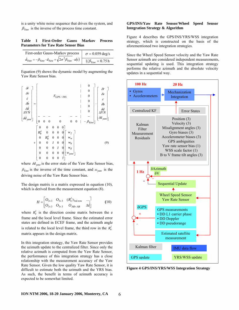
GPS/INS/Yaw Rate Sensor/Wheel Speed Sensor Integration Strategy & Algorithm Figure 4 describes the GPS/INS/YRS/WSS integration strategy, which is constructed on the basis of the aforementioned two integration strategies. Since the Wheel Speed Sensor velocity and the Yaw Rate Sensor azimuth are considered independent measurements, sequential updating is used. This integration strategy performs the relative azimuth and the absolute velocity updates in a sequential way.

Figu

20 Hz

• •

G

z

M

100 H

re 4 GPS/INS/YRS/WSS In


+

-

Kalman filter

δGPS

-+

Gyros Accelerometers

PS update YR

s

PosiVelo

MisalignmGyro b

AcceleromGPS am

Yaw rate sWSS sca

B to V fram

Kalman Filter

easurementResiduals

δAzimuthδV1 Hz

Sequential Up

Wheel SpeedYaw Rate S

GPS measurem• DD L1 carri• DD Doppler• DD pseudora

Estimated smeasurem

Error State
Centralized KF
tion (3) city (3) ent angles (3) iases (3)

eter biases (3) biguities

ensor bias (1) le factor (1) e tilt angles (3)

date

Sensor ensor

ents er phase nge

atellite ent
IMU data flow
tegration Strategy

S/WSS update


The Measurement Accuracy of GPS, Wheel Speed Sensor & Yaw Rate Sensor Using the NovAtel OEM2 precise velocity GPS receiver that provides millimeter per second level accuracy, the Wheel Speed Sensor measurement accuracy was determined in a specially conducted kinematic test. By driving the car at low (20 km/h), medium (50 km/h) and high (80 km/h) speeds on a flat road and in a straight direction, the speed error between the Wheel Speed Sensor and OEM2 GPS velocity receiver can be computed and the Wheel Speed Sensor measurement accuracy can be estimated accordingly. The measurement accuracy of the Yaw Rate Sensor as well as the first-order Gauss-Markov process parameters of the Yaw Rate Sensor bias shown in Table 1 were determined by a long time static test. In static mode, the Yaw Rate Sensor measures the Earth rotation rate. To avoid the long term variations in the data, 40 evenly spaced 1-second intervals were chosen, and the corresponding standard deviation of each interval was calculated. The average standard deviation across all intervals is computed as the accuracy of the Yaw Rate Sensor. The first-order Gauss-Markov process parameters were estimated from the autocorrelation series by using a least square curve fitting technique. The autocorrelation series were computed from the low-frequency components in the wavelet decomposition of the long time static dataset. Table 2 summarizes the measurement accuracy of GPS, the Wheel Speed Sensor as well as the Yaw Rate Sensor. In this table, GPS has the highest accuracy. During GPS outages, the Wheel Speed Sensor has a relatively high accuracy. Since the Yaw Rate Sensor used in this research is automotive grade, it has a lower accuracy.

Table 2 Measurement Accuracy of GPS, Wheel Speed Sensor and Yaw Rate Sensor

GPS Carrier phase: 5 cm

Doppler: 3 cm/s Pseudorange: 50 cm

Wheel Speed Sensor 5 cm/s Yaw Rate Sensor 0.408 deg/s

Kalman filter performs the measurement update in terms of the measurement accuracy. When GPS is fully available, GPS dominates in the Kalman filter due to its high absolute accuracy. Consequently, in this case, the three integration strategies produce almost equivalent results to GPS/INS integrated system. During GPS outages however, the Wheel Speed Sensor with a relatively high accuracy dominates in the Kalman filter. In contrast, the low quality Yaw Rate Sensor, combined with the fact that it only provides relative azimuth

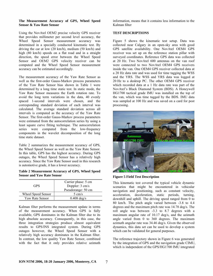
information, means that it contains less information to the Kalman filter TEST DESCRIPTIONS Figure 5 shows the kinematic test setup. Data was collected near Calgary in an open-sky area with good GPS satellite availability. One NovAtel OEM4 GPS receiver was set up on the reference station pillar with surveyed coordinates. Reference GPS data was collected at 20 Hz. Two NovAtel 600 antennas on the van roof were connected to two NovAtel OEM4 GPS receivers inside the van. One OEM4 GPS receiver collected data at a 20 Hz data rate and was used for time tagging the WSS and the YRS. The WSS and YRS data was logged at 20 Hz to a desktop PC. The other OEM4 GPS receiver which recorded data at a 1 Hz data rate was part of the NovAtel’s Black Diamond System (BDS). A Honeywell HG1700 tactical grade IMU was installed on the top of the van, which was time tagged by the BDS. IMU data was sampled at 100 Hz and was saved on a card for post processing.

Figure 5 Field Test Descrip

This kinematic test coveredscenarios that might be navigation and positioning,acceleration, deceleration, downhill and uphill. The dri80 km/h. The pitch angle degrees and the maximum piroll angle was between -3maximum angular rate of 1angle varied from 0 to 3azimuth angular rate was 34.dynamics, this data set can which can be validated for ge The reference trajectory showby the integration of GPS anwhich is independent of the G

Antennas HG1700 IMU n

e

Test van and base statio

Open sky
Vehicle sensor cabl
tion

the typical vehicle dynamic encountered in vehicular

such as constant velocity, static periods, turning,

ving speed ranged from 0 to varied between -3.8 to 4.4 tch rate was 14.78 deg/s. The .3 to 8.7 degrees with a

0.17 deg/s, and the azimuth 60 degrees. The maximum 46 deg/s. Given the observed be used to develop a system neral purposes.

n in Figure 6 was generated d the navigation grade CIMU,

PS/HG1700 IMU integrated


system. The GPS/CIMU integrated data was processed by the PosPac software from the Applanix Corporation. PosPac can compute the optimally accurate and the backward smoothed navigation solution. The accuracy estimates output from the software indicate that the solution is better than 1.4 cm horizontally, and 5.5 cm vertically. To evaluate the effects of the integration strategies during GPS outages, four GPS outages were simulated. Each outage has durations of 10, 20, 30 and 40 s. Figure 7 through Figure 10 show the vehicle dynamics during each individual GPS outage. Among these four simulated GPS outages, outage 1 and 3 are with slow varying vehicle dynamics as shown in Figure 7 and Figure 9, and the other two (Figure 8 and Figure 10) cover a wide range of vehicle dynamics, such as acceleration, deceleration and constant speed, as well as attitude orientation changes such as turning, constant azimuth as well as pitch and roll changes. The locations of the outages on the reference trajectory are labeled on Figure 6.

Figure 6 Reference Trajectory

Figure 7 Vehicle Dynamics With Respect to GPS Outage 1

Figure 8 Vehicle Dynamics with Respect to GPS Outage 2

Figure 9 Vehicle Dynamics with Respect to GPS Outage 3

Figure 10 Vehicle Dynamics with respect to GPS Outage 4

2 1 3 4


RESULTS AND ANALYSIS The performance of each integration strategy is analyzed in two ways. First, the position and velocity drift errors relative to the reference trajectory during the four simulated 40 s GPS outages are evaluated. Comparing the behavior of the integration strategies can indicate if any benefit can be gained from WSS or YRS during GPS outages. Additionally, the estimated position and velocity standard deviations, which come from the updated covariance matrix in the Kalman filter, are an estimate of the actual error by the Kalman filter, which should have good agreement with the actual error in an ideal case. In practice, however, it indicates that the model and parameters in the Kalman filter are well tuned if the estimated standard deviation does not deviate too much from the variation of the actual error. Furthermore, the estimated standard deviation determines the search space for ambiguity resolution which has a direct relationship with the ambiguity resolution time. From this point of view, the actual position and velocity error, as well as their estimated standard deviations, are analyzed during GPS outages. By computing the error relative to the reference solution, the RMS error across all the outages is examined. The average estimated standard deviation across all of the outages is also computed. Second, when GPS is restored from a full outage, the time to fix the ambiguities, as well as the correctness of the selected integers, are investigated. The average time to fix ambiguities corresponding to GPS-only, GPS/INS tight coupling as well as each individual integration strategy were computed after each simulated GPS outage. For the data processed herein, correct ambiguities were always selected. Position & Velocity Drift Error During GPS Outages Figure 11 through Figure 13 compare the position RMS errors and the average estimated standard deviations of the three integration strategies to the corresponding values from the GPS/INS solution. The velocity results can be inferred from the position results and are therefore not shown. Table 3 and Table 4 summarize the RMS position and velocity drift error as well as the average estimated standard deviation at the end of the 40 s GPS outage. Table 5 evaluates the position and velocity drift error percentage improvement of the proposed integration strategies over GPS/INS tight coupling strategy. In Figure 11, the RMS position error and average estimated standard deviation of the inertial plus Wheel Speed Sensor is much smaller than that of the free-inertial system. From Table 3, the free-inertial system horizontal RMS position error of 2.189 m and velocity error of 0.123 m/s at the end of the 40 s GPS outage can be reduced to 0.329 m and 0.028 m/s by using the inertial

plus Wheel Speed Sensor system, which yields an 85.0% and 77.2% improvement respectively. Since the Wheel Speed Sensor does not provide any aiding in the up direction, no improvement can be found. The 3D position drift error can be reduced from 2.207 m for the free-inertial system to 0.455 m through the integration with the Wheel Speed Sensor, and the 3D velocity drift error can be reduced from 0.124 m/s to 0.030 m/s. The 3D position percentage improvement is 79.4%, and the velocity percentage improvement is 75.8%. Therefore, the Wheel Speed Sensor greatly enhances the system accuracy during GPS outages when it is suitably integrated with GPS and INS. Similarly, the average estimated standard deviation is also reduced when integrating the Wheel Speed Sensor. In the meantime, with respect to the actual 3D position and velocity errors of 0.455 m and 0.030 m/s respectively, the average estimated 3D position and velocity errors are at 1.523 m and 0.073 m/s. The RMS actual error and the average estimated standard deviation with respect to the four simulated GPS outages agree reasonably well even though some differences exist due to the limited sample of the simulated outages.

Figure 11 Position RMS Error and Average Estimated Standard Deviation for Four GPS Outages (GPS/INS/WSS Integration Strategy)

Figure 12 compares the position RMS errors and the average standard deviations between the GPS/INS/YRS and GPS/INS tight coupling strategies. Their average estimated standard deviations virtually overlap. With this in mind, it makes sense that the actual position and velocity RMS error of the GPS/INS/YRS system is only slightly smaller than that of the free-inertial system. The RMS horizontal position and velocity error of the free-inertial system are reduced 8.6% and 3.3% respectively, from 2.189 m and 0.123 m/s to 2.001 m and 0.119 m/s. The 3D RMS position and velocity error are reduced 8.4% and 4.0% respectively, from 2.207 m and 0.124 m/s of the free-inertial system to 2.021 m and 0.119 m/s of inertial plus Yaw Rate Sensor system. Compared to the


GPS/INS/WSS integration strategy, GPS/INS/YRS reduces the position and velocity drift error to a much smaller degree. It again shows that the Yaw Rate Sensor has less weight in the Kalman filter due to its low measurement accuracy. Thus, the overall improvement from the Yaw Rate Sensor is less significant than with the Wheel Speed Sensor. Table 3 Position and Velocity RMS Error at the End of 40 s GPS Outage

RMS error at the end of 40 s GPS outage Strategies

Horizontal Up 3D Position [m]

GPS/INS 2.189 0.283 2.207 GPS/INS/WSS 0.329 0.314 0.455 GPS/INS/YRS 2.001 0.282 2.021

GPS/INS/YRS/WSS 0.310 0.313 0.441 Velocity [m/s]


GPS/INS/YRS/WSS 0.027 0.010 0.029

Figure 12 Position RMS Error and Average Estimated Standard Deviation for Four GPS Outages (GPS/INS/YRS Integration Strategy)

Since the GPS/INS/YRS/WSS integration strategy relies on the Wheel Speed Sensor to a larger degree than the Yaw Rate Sensor, the RMS actual and the average estimated errors are largely reduced by Wheel Speed Sensor with a slight further reduction by the sequential integration of the Yaw Rate Sensor. Comparing Figure 11 and Figure 13, the horizontal RMS and 3D position error of the GPS/INS/WSS integration strategy at the end of the 40 s GPS outage can be slightly reduced from 0.329 m and 0.455 m to 0.310 m and 0.441 m respectively through the addition of the Yaw Rate Sensor. Accordingly, the horizontal and 3D position error percentage improvement

of GPS/INS/WSS integration strategy over GPS/INS can be marginally increased from 85.0% and 79.4% to 85.8% and 80.0% by the GPS/INS/YRS/WSS strategy.

Figure 13 Position RMS Error and Average Estimated Standard Deviation for Four GPS Outages (GPS/INS/YRS/WSS Integration Strategy)

Table 4 Position and Velocity Average Estimated Standard Deviation at the End of 40 s GPS Outage

Average estimated standard deviation at the end of 40 s

GPS outage Strategies

Horizontal Up 3D Position [m]


GPS/INS/YRS/WSS 0.862 1.255 1.523 Velocity [m/s]


GPS/INS/YRS/WSS 0.052 0.05 0.072

Table 5 Position and Velocity Error Percentage Improvement of Three Integration Strategies over GPS/INS Tight Coupling Strategy

Strategies Horizontal 3D Position [%]

GPS/INS/WSS 85.0 79.4 GPS/INS/YRS 8.6 8.4

GPS/INS/YRS/WSS 85.8 80.0 Velocity [% ]

GPS/INS/WSS 77.2 75.8 GPS/INS/YRS 3.3 4.0

GPS/INS/YRS/WSS 78.1 76.6


Time to Fix Ambiguities after GPS Outages The ambiguity resolution time is determined by the search volume, which is closely related to the covariance of the estimated ambiguities. It has been shown theoretically in Scherzinger (2002), and verified by Petovello (2003) as well as Zhang et al. (2005), that an external measurement update such as an inertial measurement can reduce the covariance of the estimated ambiguities and, as a result, some benefits can be gained in the time to fix ambiguities after GPS outages. More specifically, from the above analysis on the position and velocity drift error and the average estimated standard deviation during GPS outages, the external velocity update from the Wheel Speed Sensor significantly reduces the estimated standard deviation and makes the ambiguity search space smaller. Therefore, the time to fix ambiguities can be reduced for any integration strategy that contains the Wheel Speed Sensor. In other words, the Wheel Speed Sensor can benefit significantly in reducing the time to fix ambiguities after GPS outages. Figure 14 shows the time to fix ambiguities for the GPS-only, GPS/INS tight coupling and GPS/INS/WSS strategies after four simulated GPS outages that last 10 s, 20 s, 30 s and 40 s. Table 6 and Table 7 show the percentage improvement in the average time to fix ambiguities over GPS-only as well as GPS/INS tight coupling for all integration strategies and all GPS outage durations. With respect to GPS-only, corresponding to the fourth GPS outage, the time to fix ambiguities after 10 s is much larger than other scenarios. The possible reason to account for this is that a 2.5 m/s2 acceleration in the East direction as well as a 14 deg/s azimuth rate occurred simultaneously between 0 and 10 s during the fourth GPS outages. The detailed vehicle dynamics can be found in Figure 10. The high vehicle dynamics may insert some influences on the time to fix ambiguities. When integrating the Wheel Speed Sensor with GPS/INS system, the percentage improvement over GPS-only reaches 94.5 %, 44.8%, 20.7% and 11.3%. By contrast, the percentage improvement over GPS/INS tight coupling reaches 7.1%, 6.7 %, 5.1% and 4.1 %. From Petovello (2003) and Zhang et al.(2005), the INS does not provide significant improvement over the GPS-only case after about 30 seconds of GPS outages. Therefore, for the shorter GPS outages, both INS and WSS contribute to the improvement on the time to fix ambiguities over GPS-only. For outage durations that are larger than 30 s, the improvements are less significant than a shorter time period of GPS outages. Nevertheless, the addition of the WSS does provide some benefit. Figure 15 compares the time to fix ambiguities after 10 s, 20 s, 30 s and 40 s GPS outages for a GPS-only, GPS/INS

tight coupling and GPS/INS/YRS integration strategies. The GPS/INS/YRS strategy improves the time to fix ambiguities over the GPS-only strategy to a larger degree for a shorter GPS outage, and to a smaller degree for a longer GPS outage. Comparing between the GPS/INS/YRS and GPS/INS tight coupling integration strategies, since the estimated standard devations of GPS/INS/YRS and GPS/INS tight coupling are almost identical, no significant benefit in the time to fix ambiguities can be expected from the Yaw Rate Sensor integration strategy even if the GPS outage time is less than 30 s. This means the Yaw Rate Sensor contributes less to the improvement of time to fix ambiguities over the GPS/INS tight coupling strategy.

Figure 14 Time to Fix of Ambiguities after 10 s, 20 s, 30 s, 40 s GPS Outages for GPS-only, GPS/INS Tight Coupling and GPS/INS/WSS Integration Strategy

Figure 15 Time to Fix Ambiguities after 10 s, 20 s, 30 s, 40 s GPS Outages for GPS-only, GPS/INS Tight Coupling and GPS/INS/YRS Integration Strategy

For the GPS/INS/YRS/WSS integration strategy that is dominated by the Wheel Speed Sensor, its position


average estimated standard deviations shown in Table 4 are same as those for the GPS/INS/WSS integration strategy. From this point of view, it makes sense that the times to fix ambiguities after GPS outages shown in Figure 16 for the GPS/INS/YRS/WSS integration strategy are all basically the same as for the GPS/INS/WSS integration strategy shown in Figure 14.

Figure 16 Time to Fix Ambiguities after 10 s, 20 s, 30 s, 40 s GPS Outages for GPS-only, GPS/INS Tight Coupling and GPS/INS/YRS/WSS Integration Strategy

Table 6 Average Time to Fix Ambiguities Percentage Improvement of Three Integration Strategies over GPS-only

Durations of GPS outages Strategies 10 s 20 s 30 s 40 s

GPS/INS/WSS 94.5 44.8 20.7 11.3 GPS/INS/YRS 94.1 40.8 16.7 8.1

GPS/INS/YRS/WSS 94.6 44.8 20.7 11.3

Table 7 Average Time to Fix Ambiguities Percentage Improvement of Three Integration Strategies over GPS/INS Tight Coupling

Durations of GPS outages Strategies 10 s 20 s 30 s 40 s

GPS/INS/WSS 7.1 6.7 5.1 4.1 GPS/INS/YRS 0 0 0 0.7

GPS/INS/YRS/WSS 7.1 6.7 5.1 4.1 CONCLUSIONS Using a centralized processing approach, three integration strategies are proposed by integrating the Wheel Speed Sensor (WSS) and Yaw Rate Sensor (YRS) with GPS/INS in various combinations, namely GPS/INS/WSS, GPS/INS/YRS and GPS/INS/YRS/WSS. The WSS scale factor, the tilt angles between the b and v frames as well

as the YRS scale factor are augmented to the error states of a centralized Kalman filter. When GPS is fully available, GPS dominates in the Kalman filter, and the three integration strategies produce almost equivalent results to the GPS/INS integrated system. During GPS outages, the benefits gained by integrating on-board vehicle sensors are reductions in the position and velocity errors as well as an improvement in the time to fix ambiguities. Improvements in the position and velocity errors are closely related to the sensor measurement accuracy. The Wheel Speed Sensor with high measurement accuracy outweighs the Yaw Rate Sensor with lower quality, and hence provides the most benefit. The Wheel Speed Sensor greatly enhances the system accuracy during GPS outages. The reduction of the actual and estimated errors resulting from the Yaw Rate Sensor is less significant than with the Wheel Speed Sensor. The estimated standard deviation has a direct relationship with the time to fix ambiguities. The Wheel Speed Sensor significantly reduces the estimated standard deviation and makes the ambiguity search space smaller. The time to fix ambiguities can be reduced to a large degree for any integration strategy that contains the Wheel Speed Sensor. The estimated standard devations of the GPS/INS/YRS and GPS/INS tight coupling approaches are almost identical. No significant benefit in the time to fix ambiguities were obtained from the Yaw Rate Sensor. REFERENCES Bevly, D.M.(1999) Evaluation of a Blended Dead

Reckoning and Carrier Phase Differential GPS System for Control of an Off-Road Vehicle. Proceedings of ION GPS 1999. (September, Nashville, TN), pp. 2061-2069.

Harvey, R.S. (1998). Development of a Precision pointing System Using an Integrated Multi-Sensor Approach. M.Sc. thesis, UCGE Report, Department of Geomatics Engineering, University of Calgary.

Hay, C. (2005) Turn, Turn, Turn Wheel-Speed Dead Reckoning for Vehicle Navigation. GPS World, October, 2005, pp 37-42.

Jekli, C. (2000) Inertial Navigation Systems with Geodetic Applications. Walter de, Gruyter, New York, NY, USA.

Kubo, J., Kindo, T., Ito, A. and Sugimoto, S. (1999) DGPS/INS/Wheel Sensor Integration for High Accuracy Land-Vehicle Positioning. Proceedings of ION GPS 1999. (September, Nashville, TN), pp. 555-564.


Petovello, M.G. (2003) Real-Time Integration of Tactical Grade IMU and GPS for High-Accuracy Positioning and Navigation. PhD Thesis, UCGE Report #20116, Department of Geomatics Engineering, University of Calgary.

Redmill, K.A., Kitajima, T. and Ozguner, U. (2001) DGPS/INS Integrated Positioning for Control of Automated Vehicle. IEEE Intelligent Transportation Systems Conference Proceedings. (August, Oakland, CA), pp. 172-178.

Scherzinger, B.M. (2002). Robust Positioning with Single Frequency Inertially Aided RTK. Proceedings of ION NTM 2002 (January, Alexandria, VA, USA). pp. 911-917.

Stephen, J. (2000). Development of a Multi-Sensor GNSS Based Navigation system. M.S.c. Thesis, UCGE Report, Department of Geomatics Engineering, University of Calgary

Sukkarieh, S. (2000) Low Cost, High Integrity, Aided Inertial Navigation System for Autonomous Vehicles. Ph.D Thesis, Australian Center for Field Robotics, University of Sydney, Australia.

Tseng, H.E., Ashrafi, B.,Madau, D., Brown, T.A. and Recker,D. (1999) The Development of Vehicle Stability Control at Ford. IEEE/ASME Transactions on Mechatronics, Vol.4, No.4, 1999, pp. 223-234.

Wang, C.C. (1998) Development of a Low-cost GPS-based Attitude Determination System. M.Sc. thesis, UCGE Report #20175, Department of Geomatics Engineering, University of Calgary.

Zhang, H.T., Petovello, M.G. and Cannon, M.E.(2005) Performance Comparison of Kinematic GPS Integrated with Different Tactical Level IMUs. Proceedings of ION NTM 2005, (January, San Diego, CA), pp. 243-254.

development of precise gps/ins/wheel speed … ntm 2006, 18-20 january 2006, monterey, ca 1...

Documents