development of robust document analysis and recognition ...jinesh/ocrdesigndoc.pdf · development...
TRANSCRIPT
OCR Technical Report
for the project
Development of Robust
Document Analysis and Recognition
System for Printed
Indian Scripts
Project Sponsered By
Ministry of Communication and Information Technology
July 2008

This document has been written with contributions from:
1. IIIT Hyderabad
2. University of Hyderabad
3. Punjabi University, Patiala
4. Utkal University, Bhubneshwar
5. IIIT Allahabad
6. M.S. University, Baroda
7. ISI Kolkatta
8. IISc Bangalore
9. C-DAC Noida
10. IIT Delhi
Document compiled and edited by:
− Prof. Santanu Chaudhury(Project Investigator, IIT Delhi)
− Ritu Garg(Project Associate, IIT Delhi)

Contents
List of Figures ix
List of Tables xv
1 Problems of OCR Development in Indian Scripts 11.1 Devanagari Script . . . . . . . . . . . . . . . . . . . . . . . . . . . . . . . 11.2 Bangla Script . . . . . . . . . . . . . . . . . . . . . . . . . . . . . . . . . 21.3 Malayalam Script . . . . . . . . . . . . . . . . . . . . . . . . . . . . . . . 6
1.3.1 Technical characteristics . . . . . . . . . . . . . . . . . . . . . .. 71.3.2 Independent vowels and Dependent vowel signs . . . . . . .. . . . 91.3.3 Script Revision . . . . . . . . . . . . . . . . . . . . . . . . . . . . 101.3.4 Challenges . . . . . . . . . . . . . . . . . . . . . . . . . . . . . . 10
1.4 Gurmukhi Script . . . . . . . . . . . . . . . . . . . . . . . . . . . . . . . 101.4.1 Challenges in Developing Gurmukhi OCR . . . . . . . . . . . . .14
1.5 Tibetan and Nepali Script . . . . . . . . . . . . . . . . . . . . . . . . . .. 191.6 Oriya Script . . . . . . . . . . . . . . . . . . . . . . . . . . . . . . . . . . 221.7 Kannada Script . . . . . . . . . . . . . . . . . . . . . . . . . . . . . . . . 231.8 Gujarati Script . . . . . . . . . . . . . . . . . . . . . . . . . . . . . . . . . 231.9 Telugu Script . . . . . . . . . . . . . . . . . . . . . . . . . . . . . . . . . 26
1.9.1 Script Characteristics . . . . . . . . . . . . . . . . . . . . . . . . .261.9.2 Component Definition . . . . . . . . . . . . . . . . . . . . . . . . 27
1.10 General OCR problems . . . . . . . . . . . . . . . . . . . . . . . . . . . . 281.10.1 Imaging Defects . . . . . . . . . . . . . . . . . . . . . . . . . . . 281.10.2 Similar Symbols . . . . . . . . . . . . . . . . . . . . . . . . . . . 291.10.3 Punctuation . . . . . . . . . . . . . . . . . . . . . . . . . . . . . . 301.10.4 Typography . . . . . . . . . . . . . . . . . . . . . . . . . . . . . . 30
1.11 Possible Directions . . . . . . . . . . . . . . . . . . . . . . . . . . . . .. 321.11.1 Image processing . . . . . . . . . . . . . . . . . . . . . . . . . . . 32
i
1.11.2 Adaptation . . . . . . . . . . . . . . . . . . . . . . . . . . . . . . 33
1.11.3 Multi-character recognition . . . . . . . . . . . . . . . . . . .. . 34
1.11.4 Linguistic context . . . . . . . . . . . . . . . . . . . . . . . . . . . 34
2 Software Architecture of OCR System 37
2.1 Stage 1 : Image Acquisition . . . . . . . . . . . . . . . . . . . . . . . . .38
2.1.1 Image Acquisition: XML Input Specifications . . . . . . . . . . . . 38
2.1.2 Image Acquisition: XML Output Specifications . . . . . . . . . . . 41
2.2 Stage 2: Pre-Processing Scanned Document Images . . . . . .. . . . . . . 43
2.2.1 Pre-Processing: XML Input Specifications . . . . . . . . . . . . . 43
2.2.2 Pre-Processing: XML Output Specifications . . . . . . . . . . . . 43
2.3 Stage 3: Script Independent Processing . . . . . . . . . . . . . .. . . . . 46
2.3.1 Script Independent Processing: XML Input Specifiations . . . . . . 46
2.3.2 Script Independent Processing: XML Output Specifications . . . . 46
2.4 Stage 4: Script Dependent Processing . . . . . . . . . . . . . . . .. . . . 48
2.4.1 Script Dependent Processing: XML Input Specifications . . . . . . 48
2.4.2 Script Dependent Processing: XML Output Specifications . . . . . 49
2.4.3 Script Dependent Processing: XML output specifications for Sub-Modules . . . . . . . . . . . . . . . . . . . . . . . . . . . . . . . 50
2.5 Stage 5: User Interface . . . . . . . . . . . . . . . . . . . . . . . . . . . .53
2.5.1 User Interface: XML Input Specifiations . . . . . . . . . . . . . . 53
2.5.2 User Interface: XML input schema . . . . . . . . . . . . . . . . . 54
3 Pre-processing of Scanned Documents 59
3.1 Introduction . . . . . . . . . . . . . . . . . . . . . . . . . . . . . . . . . . 59
3.2 Text Direction : Detection and correction of portrait/landscape mode . . . 60
3.2.1 Requirement analysis . . . . . . . . . . . . . . . . . . . . . . . . . 60
3.2.2 Software development . . . . . . . . . . . . . . . . . . . . . . . . 60
3.3 Skew Detection and correction . . . . . . . . . . . . . . . . . . . . . .. . 62
3.4 Noise Removal . . . . . . . . . . . . . . . . . . . . . . . . . . . . . . . . 63
3.5 Binarization and Thresholding . . . . . . . . . . . . . . . . . . . . .. . . 63
3.5.1 Sauvola Binarization Module - ISI Kolkatta . . . . . . . . .. . . . 64
3.5.2 The Adaptive and Quadratic Preprocessor : IIT Delhi . .. . . . . . 65
3.5.3 Thresholding Techniques . . . . . . . . . . . . . . . . . . . . . . . 68
3.6 Cropping . . . . . . . . . . . . . . . . . . . . . . . . . . . . . . . . . . . 70
ii
4 Script-Independent Processing : Segmentation and LayoutAnalysis 714.1 Document Image Segmentation . . . . . . . . . . . . . . . . . . . . . . .. 71
4.1.1 Recursive X-Y Cut . . . . . . . . . . . . . . . . . . . . . . . . . . 714.1.2 Docstrum . . . . . . . . . . . . . . . . . . . . . . . . . . . . . . . 724.1.3 Profile Based Page Segmentation . . . . . . . . . . . . . . . . . . 72
4.2 Top-Down Scheme for Multi-page Document Segmentation .. . . . . . . 774.2.1 Top-down Segmentation using Document Schema . . . . . . .. . 85
4.3 Content Classification . . . . . . . . . . . . . . . . . . . . . . . . . . . .. 864.3.1 Estimating Globally Matched Wavelet filters . . . . . . . .. . . . 864.3.2 Locating text from arbitrary backgrounds . . . . . . . . . .. . . . 904.3.3 Classification . . . . . . . . . . . . . . . . . . . . . . . . . . . . . 914.3.4 Segmentation of document images . . . . . . . . . . . . . . . . . .934.3.5 MRF postprocessing for Document Image Segmentation .. . . . . 954.3.6 Document Image Segmentation . . . . . . . . . . . . . . . . . . . 97
4.4 Results and Comparisons . . . . . . . . . . . . . . . . . . . . . . . . . . .98
5 Script-Dependent Processing : Unicode Generation 1055.1 Architecture of Script Dependent OCR module . . . . . . . . . .. . . . . 106
6 Telugu OCR System: Classifier Design and Implementation 1096.1 Language structure based clustering . . . . . . . . . . . . . . . .. . . . . 1096.2 Convolutional Neural Network classifier . . . . . . . . . . . . .. . . . . . 110
6.2.1 Convolutional neural networks . . . . . . . . . . . . . . . . . . .. 1116.2.2 LeCun’s architecture — LeNet-5 — for recognizing handwritten
Roman numerals . . . . . . . . . . . . . . . . . . . . . . . . . . . 1126.3 Multi-class C-NN Classifier for Telugu Components . . . . .. . . . . . . 113
6.3.1 Architecture – 1 . . . . . . . . . . . . . . . . . . . . . . . . . . . . 1146.3.2 Hybrid architecture for 44-class problem . . . . . . . . . .. . . . 116
6.4 Other Experiments . . . . . . . . . . . . . . . . . . . . . . . . . . . . . . 1206.4.1 Normalizing stroke-widths of components . . . . . . . . . .. . . . 1206.4.2 Clustering based on component areas . . . . . . . . . . . . . . .. 1206.4.3 EM-based binarization . . . . . . . . . . . . . . . . . . . . . . . . 121
7 Tibetan OCR System: Classifier Design and Implementation 1237.1 Introduction . . . . . . . . . . . . . . . . . . . . . . . . . . . . . . . . . . 1237.2 Description of Tibetan script: . . . . . . . . . . . . . . . . . . . . .. . . . 1237.3 Segmentation . . . . . . . . . . . . . . . . . . . . . . . . . . . . . . . . . 126
7.3.1 Line segmentation . . . . . . . . . . . . . . . . . . . . . . . . . . 127
iii
7.3.2 Word segmentation . . . . . . . . . . . . . . . . . . . . . . . . . . 1277.3.3 Checking for numerals and khari pai . . . . . . . . . . . . . . . .. 1287.3.4 Identification of the rows of the word that contain the shirorekha . . 1287.3.5 Identification of the syllable markers in the word . . . .. . . . . . 1297.3.6 Segmentation of the vowel symbols lying above the shirorekha in
the word . . . . . . . . . . . . . . . . . . . . . . . . . . . . . . . 1297.3.7 Segmentation of the symbols lying below the shirorekha . . . . . . 129
7.4 Features used for classification . . . . . . . . . . . . . . . . . . . .. . . . 1307.5 Classifier . . . . . . . . . . . . . . . . . . . . . . . . . . . . . . . . . . . 131
7.5.1 k – nearest neighbor classifier . . . . . . . . . . . . . . . . . . . .1327.5.2 Adaptive linear discriminant function classifier . . .. . . . . . . . 132
7.6 Post-processing: . . . . . . . . . . . . . . . . . . . . . . . . . . . . . . . .1347.7 Hierarchical classifier . . . . . . . . . . . . . . . . . . . . . . . . . . .. . 1357.8 Current status . . . . . . . . . . . . . . . . . . . . . . . . . . . . . . . . . 1367.9 Introduction . . . . . . . . . . . . . . . . . . . . . . . . . . . . . . . . . . 1397.10 Technical details . . . . . . . . . . . . . . . . . . . . . . . . . . . . . . .139
7.10.1 Procedure Followed . . . . . . . . . . . . . . . . . . . . . . . . . 1397.10.2 Classification Based on the Features . . . . . . . . . . . . . .. . . 1397.10.3 Feature Extraction Technique . . . . . . . . . . . . . . . . . . .. 1427.10.4 Feature Matching: (Interim step) . . . . . . . . . . . . . . . .. . . 142
7.11 Future Work . . . . . . . . . . . . . . . . . . . . . . . . . . . . . . . . . . 1437.12 Issues in Oriya OCR . . . . . . . . . . . . . . . . . . . . . . . . . . . . . 143
8 Gurmukhi OCR System: Classifier Design and Implementation 1458.1 Introduction . . . . . . . . . . . . . . . . . . . . . . . . . . . . . . . . . . 1458.2 Word Segmentation . . . . . . . . . . . . . . . . . . . . . . . . . . . . . . 1488.3 Work Skew . . . . . . . . . . . . . . . . . . . . . . . . . . . . . . . . . . 149
8.3.1 Phase 1: Skewed word identification . . . . . . . . . . . . . . . .. 1518.3.2 Phase 2: Skew Correction . . . . . . . . . . . . . . . . . . . . . . 1528.3.3 Experimental results . . . . . . . . . . . . . . . . . . . . . . . . . 153
8.4 Repairing the Word Shape . . . . . . . . . . . . . . . . . . . . . . . . . . 1548.5 Repairing Broken Characters . . . . . . . . . . . . . . . . . . . . . . .. . 1558.6 Algorithm . . . . . . . . . . . . . . . . . . . . . . . . . . . . . . . . . . . 158
8.6.1 Experiments . . . . . . . . . . . . . . . . . . . . . . . . . . . . . 1608.6.2 Algorithm . . . . . . . . . . . . . . . . . . . . . . . . . . . . . . . 164
8.7 Advantages of Combining Multiple Feature extractors and classifiers . . . . 1648.7.1 Experiments . . . . . . . . . . . . . . . . . . . . . . . . . . . . . 166
iv
9 Gujarati Script Dependent Module for OCR 1679.1 Status of Development : . . . . . . . . . . . . . . . . . . . . . . . . . . . .167
10 Kannada Recognition - Technical Report 17110.1 Introduction . . . . . . . . . . . . . . . . . . . . . . . . . . . . . . . . . . 171
10.2 Segmentation . . . . . . . . . . . . . . . . . . . . . . . . . . . . . . . . . 171
10.2.1 Line segmentation . . . . . . . . . . . . . . . . . . . . . . . . . . 171
10.2.2 Word and character segmentation . . . . . . . . . . . . . . . . .. 173
10.2.3 Akshara demarcation . . . . . . . . . . . . . . . . . . . . . . . . . 174
10.3 Character classification . . . . . . . . . . . . . . . . . . . . . . . . .. . . 174
10.4 Graph based Representation for components . . . . . . . . . .. . . . . . . 176
10.5 Similarity of the Components . . . . . . . . . . . . . . . . . . . . . .. . . 178
10.6 The Classification strategy . . . . . . . . . . . . . . . . . . . . . . .. . . 179
10.6.1 Training . . . . . . . . . . . . . . . . . . . . . . . . . . . . . . . . 180
10.6.2 Prediction . . . . . . . . . . . . . . . . . . . . . . . . . . . . . . . 181
10.6.3 Spline Features . . . . . . . . . . . . . . . . . . . . . . . . . . . . 181
10.7 Experiments, Results and Discussions . . . . . . . . . . . . . .. . . . . . 183
10.7.1 Data Set . . . . . . . . . . . . . . . . . . . . . . . . . . . . . . . . 183
10.7.2 Pre-processing . . . . . . . . . . . . . . . . . . . . . . . . . . . . 184
10.7.3 Feature extraction . . . . . . . . . . . . . . . . . . . . . . . . . . . 184
10.7.4 Experiments and discussions . . . . . . . . . . . . . . . . . . . .. 184
10.8 Conclusion . . . . . . . . . . . . . . . . . . . . . . . . . . . . . . . . . . 191
11 Bangla OCR System 19311.1 Introduction . . . . . . . . . . . . . . . . . . . . . . . . . . . . . . . . . . 193
11.2 Skew detection and Correction algorithm . . . . . . . . . . . .. . . . . . 193
11.3 Classification of mid-zone characters and modifier symbols . . . . . . . . . 194
11.4 Two Stage Classifier . . . . . . . . . . . . . . . . . . . . . . . . . . . . . 194
12 Recognition of Malayalam Documents 19712.1 Background . . . . . . . . . . . . . . . . . . . . . . . . . . . . . . . . . . 197
12.2 OCR sytem . . . . . . . . . . . . . . . . . . . . . . . . . . . . . . . . . . 198
12.3 Ongoing Activities . . . . . . . . . . . . . . . . . . . . . . . . . . . . . .202
12.3.1 Integration of OCR system . . . . . . . . . . . . . . . . . . . . . . 203
12.4 Efficient implementation of SVM . . . . . . . . . . . . . . . . . . . .. . . 203
12.5 Ongoing and Future Activities . . . . . . . . . . . . . . . . . . . . .. . . 205
v
13 Language Resources for correcting OCR output 20713.1 Introduction . . . . . . . . . . . . . . . . . . . . . . . . . . . . . . . . . . 20713.2 Indian Scripts . . . . . . . . . . . . . . . . . . . . . . . . . . . . . . . . . 20813.3 Related Work . . . . . . . . . . . . . . . . . . . . . . . . . . . . . . . . . 20813.4 The Model (Kolak et al [1]) . . . . . . . . . . . . . . . . . . . . . . . . .21013.5 Use of Corpus for OCR post processing . . . . . . . . . . . . . . . .. . . 211
13.5.1 Gurmukhi . . . . . . . . . . . . . . . . . . . . . . . . . . . . . . . 21213.6 Conclusions . . . . . . . . . . . . . . . . . . . . . . . . . . . . . . . . . . 212
14 Software Engineering : Integration and Namespaces 21514.1 Deliverables . . . . . . . . . . . . . . . . . . . . . . . . . . . . . . . . . . 21514.2 Software Environment . . . . . . . . . . . . . . . . . . . . . . . . . . . .21514.3 System Integration . . . . . . . . . . . . . . . . . . . . . . . . . . . . . .216
14.3.1 System Integration Architecture . . . . . . . . . . . . . . . .. . . 21614.3.2 Integration Testing . . . . . . . . . . . . . . . . . . . . . . . . . . 21714.3.3 GUI Snapshots . . . . . . . . . . . . . . . . . . . . . . . . . . . . 222
14.4 Namespaces . . . . . . . . . . . . . . . . . . . . . . . . . . . . . . . . . . 222
15 ASSESSMENT OF OCR SOFTWARE 22915.1 Introduction . . . . . . . . . . . . . . . . . . . . . . . . . . . . . . . . . . 22915.2 OCR Software Testing & Quality Assessment . . . . . . . . . . .. . . . . 23015.3 Correctness testing . . . . . . . . . . . . . . . . . . . . . . . . . . . . .. 231
15.3.1 Black-box testing . . . . . . . . . . . . . . . . . . . . . . . . . . . 23115.3.2 White-box testing . . . . . . . . . . . . . . . . . . . . . . . . . . . 23215.3.3 Reliability testing . . . . . . . . . . . . . . . . . . . . . . . . . . .23315.3.4 Performance testing . . . . . . . . . . . . . . . . . . . . . . . . . 233
15.4 Performance Evaluation & Quality Metrics . . . . . . . . . . .. . . . . . 23415.4.1 Evaluation of Segmentation . . . . . . . . . . . . . . . . . . . . .23415.4.2 Evaluation of the OCR Engine . . . . . . . . . . . . . . . . . . . . 235
15.5 Efficiency . . . . . . . . . . . . . . . . . . . . . . . . . . . . . . . . . . . 236
16 Code Optimization 23716.1 Requirement Considerations for Optimization . . . . . . .. . . . . . . . . 23716.2 Steps in Optimization . . . . . . . . . . . . . . . . . . . . . . . . . . . .. 237
16.2.1 Code Analysis . . . . . . . . . . . . . . . . . . . . . . . . . . . . 23816.2.2 Implementation of optimization . . . . . . . . . . . . . . . . .. . 23816.2.3 Testing of optimized code . . . . . . . . . . . . . . . . . . . . . . 239
16.3 Tools used for optimization . . . . . . . . . . . . . . . . . . . . . . .. . . 240
vi

16.4 Future considerations and suggestions . . . . . . . . . . . . .. . . . . . . 24016.5 Current work Status . . . . . . . . . . . . . . . . . . . . . . . . . . . . . .240
17 Development of Image Corpus and Annotation 24317.1 Background . . . . . . . . . . . . . . . . . . . . . . . . . . . . . . . . . . 24317.2 Objective . . . . . . . . . . . . . . . . . . . . . . . . . . . . . . . . . . . 24317.3 Annotation Process . . . . . . . . . . . . . . . . . . . . . . . . . . . . . .24417.4 Development of Annotation Tools . . . . . . . . . . . . . . . . . . .. . . 24417.5 Current Status of Annotation Process . . . . . . . . . . . . . . .. . . . . . 24617.6 Plans and Issues . . . . . . . . . . . . . . . . . . . . . . . . . . . . . . . . 246
17.6.1 Challenges in Building of the corpus . . . . . . . . . . . . . .. . . 24817.6.2 Immediate Steps . . . . . . . . . . . . . . . . . . . . . . . . . . . 248
18 Documentation 24918.1 Introduction . . . . . . . . . . . . . . . . . . . . . . . . . . . . . . . . . . 24918.2 Documentation of Code with Doxygen . . . . . . . . . . . . . . . . .. . . 249
18.2.1 Getting Started . . . . . . . . . . . . . . . . . . . . . . . . . . . . 250
References 269
vii

List of Figures
1.1 Characters and Symbols of Devanagari Script. (courtesyreference [2]) . . 21.2 Sample Hindi text written in Devanagari script. (courtesy reference [2]) . . 21.3 Bangla Character Set . . . . . . . . . . . . . . . . . . . . . . . . . . . . . 31.4 Bangla Compound Characters . . . . . . . . . . . . . . . . . . . . . . . .41.5 Irregular Sequencing of Characters . . . . . . . . . . . . . . . . .. . . . 41.6 Errors due to Intra and Inter word Touching . . . . . . . . . . . .. . . . . 51.7 Errors due to Compound Character formation . . . . . . . . . . .. . . . . 61.8 Uncommon Typos . . . . . . . . . . . . . . . . . . . . . . . . . . . . . . 61.9 Malayalam alphabets:vowels. . . . . . . . . . . . . . . . . . . . . . .. . . 71.10 Malayalam alphabets:consonants. . . . . . . . . . . . . . . . . .. . . . . 71.11 Malayalam alphabets:Chillu characters. . . . . . . . . . . .. . . . . . . . 71.12 Vowel diacritics with ka. . . . . . . . . . . . . . . . . . . . . . . . . .. . 81.13 Conjunct Characters (Samyukthakshar). . . . . . . . . . . . .. . . . . . . 81.14 Akshara Formation: Examples. . . . . . . . . . . . . . . . . . . . . .. . . 81.15 Script Revision: Replacement of irregular ligatures.. . . . . . . . . . . . . 91.16 Script Revision: Changes in diacritics. . . . . . . . . . . . .. . . . . . . . 91.17 Script Revision: Split for Samyukthakshar. . . . . . . . . .. . . . . . . . . 101.18 Examples of Similar characters. . . . . . . . . . . . . . . . . . . .. . . . 101.19 Changes in glyph with font/ Style variation. . . . . . . . . .. . . . . . . . 111.20 Characters and symbols of Gurmukhi script . . . . . . . . . . .. . . . . . 121.21 Gurmukhi Script Word . . . . . . . . . . . . . . . . . . . . . . . . . . . . 131.22 Touching characters in Gurmukhi script . . . . . . . . . . . . .. . . . . . 141.23 Touching characters in three zones (touching parts encircled): (a) upper
zone characters touching each other, (b) upper zone characters touchingwith middle zone characters, (c) middle zone characters touching with eachother, (d) middle zone characters touching with lower zone characters, (e)lower zone characters touching with each other . . . . . . . . . . .. . . . 15
1.24 Document containing the touching characters in neighboring lines . . . . . 16
ix
1.25 Broken characters in Gurmukhi script . . . . . . . . . . . . . . .. . . . . 161.26 Extremely broken characters in Gurmukhi script . . . . . .. . . . . . . . 171.27 Broken headlines in Gurmukhi script . . . . . . . . . . . . . . . .. . . . 171.28 Heavily printed characters in Gurmukhi script . . . . . . .. . . . . . . . . 181.29 Multiple skewness in a text line . . . . . . . . . . . . . . . . . . . .. . . 191.30 Tibetan Consonants . . . . . . . . . . . . . . . . . . . . . . . . . . . . . .201.31 Tibetan Vowel . . . . . . . . . . . . . . . . . . . . . . . . . . . . . . . . 201.32 Tibetan Conjuncts . . . . . . . . . . . . . . . . . . . . . . . . . . . . . . 211.33 Tibetan Numerals . . . . . . . . . . . . . . . . . . . . . . . . . . . . . . . 211.34 Tibetan Sample Text . . . . . . . . . . . . . . . . . . . . . . . . . . . . . 211.35 Table for Gujarati Script . . . . . . . . . . . . . . . . . . . . . . . . .. . 241.36 Logical Zones . . . . . . . . . . . . . . . . . . . . . . . . . . . . . . . . . 251.37 The basic Telugu alphabet: (a) vowels, (b) consonants .. . . . . . . . . . . 261.38 Additional symbols used in creating complexaksharas: (a) semi-vowels,
(b) consonant modifiers . . . . . . . . . . . . . . . . . . . . . . . . . . . . 271.39 Examples of Simple and Compound Telugu Characters . . . .. . . . . . . 271.40 (a) and (b) Example showing a consonant modifier that is identical to the
consonant. (c) shows different positions of consonant modifiers relative tothe base character . . . . . . . . . . . . . . . . . . . . . . . . . . . . . . . 28
1.41 Problems in symbol extraction . . . . . . . . . . . . . . . . . . . . .. . . 28
2.1 Overall framewrok of end-to-end OCR . . . . . . . . . . . . . . . . .. . . 382.2 Architecture Diagram - Acquiring Images . . . . . . . . . . . . .. . . . . 392.3 GUI snapshots showing the two ways of acquiring the image. . . . . . . . 422.4 Architecture Diagram - Pre-processing Document Images. . . . . . . . . . 432.5 Shows State transitions for preprocessing module . . . . .. . . . . . . . . 452.6 GUI snapshots showing the pre-processing routines (a) Cropping routine
selection (b) Skew Detection and correction (c) Noise cleaning (d) Orien-taion routine selection . . . . . . . . . . . . . . . . . . . . . . . . . . . . . 45
2.7 Architecture Diagram - Script Independent Processing .. . . . . . . . . . 462.8 Shows state transitions for the script independent module . . . . . . . . . . 482.9 GUI snapshots showing the script independent module (a)Docstrum (b)
Image Segmentation . . . . . . . . . . . . . . . . . . . . . . . . . . . . . 482.10 Architecture Diagram - Script Dependent Processing . .. . . . . . . . . . 492.11 State transition diagram for user interface for post-OCR error correction . . 57
3.1 Result of orientation correction . . . . . . . . . . . . . . . . . . .. . . . . 613.2 Result of skew correction and detection . . . . . . . . . . . . . .. . . . . 62
x

3.3 Result of Noise cleaning . . . . . . . . . . . . . . . . . . . . . . . . . . .64
3.4 Figure shows window at (x,y) and at (x,y+1) . . . . . . . . . . . .. . . . . 65
3.5 . . . . . . . . . . . . . . . . . . . . . . . . . . . . . . . . . . . . . . . . 65
3.6 . . . . . . . . . . . . . . . . . . . . . . . . . . . . . . . . . . . . . . . . 66
3.7 Result of Binarization . . . . . . . . . . . . . . . . . . . . . . . . . . . .. 69
3.8 GUI showing cropping . . . . . . . . . . . . . . . . . . . . . . . . . . . . 70
4.1 Output of Docstrum . . . . . . . . . . . . . . . . . . . . . . . . . . . . . 73
4.2 Result of content characterization applied to documentimage. *red : back-ground, *green: picture components, *blue : textual regions . . . . . . . . . 74
4.3 Result of content classification. Regions in green indicate text and graphicgetting classified together while blue colored regions correspond to back-ground or picture region . . . . . . . . . . . . . . . . . . . . . . . . . . . 74
4.4 Text and Graphic Separation Result . . . . . . . . . . . . . . . . . .. . . 75
4.5 Result for document image with text and image . . . . . . . . . .. . . . . 76
4.6 Result for document image with text only . . . . . . . . . . . . . .. . . . 77
4.7 Result for document image Segmentation with text and graphics . . . . . . 78
4.8 Hierarchical decomposition of logical structure of a document as specifiedin XML Schema . . . . . . . . . . . . . . . . . . . . . . . . . . . . . . . . 79
4.9 Example decomposition of a Multipage Document . . . . . . . .. . . . . 80
4.10 Separable Kernel Filter Bank . . . . . . . . . . . . . . . . . . . . . . . . 87
4.11 DWT of an image( top) with its matched wavelet (bottom left) and withtraditional Haar wavelet (bottom right) . . . . . . . . . . . . . . . . . . 89
4.12 Distribution of Y for Image and Background as obtained from Classi-fier 1. Similar distributions are obtained for Classifiers 2 and 3 . . . . . 94
4.13 Document Segmentation results obtained for 2 sample imagesfromprevious section. Images show that the misclassification occurs eitherat the class boundaries or because of the presence of small isolatedclusters. . . . . . . . . . . . . . . . . . . . . . . . . . . . . . . . . . . . . 95
4.14 Results of 3 class content classification. *red : background, *green: picturecomponents, *blue : textual regions . . . . . . . . . . . . . . . . . . . .. 98
4.15 Results of showing text and graphics getting classifiedtogether . . . . . . . 99
4.16 Example of a general document image. (a) shows the original image,(b) is the image without postprocessing and (c) is the final result . . . . 100
4.17 Image with one of the three classes missing. (a) shows the originalimage, (b) is the image without postprocessing and (c) is thefinal result 100
xi

4.18 Image with text and image boundaries not well defined. (a) shows theoriginal image, (b) is the image without postprocessing and(c) is thefinal result . . . . . . . . . . . . . . . . . . . . . . . . . . . . . . . . . . 101
4.19 Document has several small chunks of image and text parts. (a) showsthe original image, (b) is the image without postprocessingand (c) isthe final result . . . . . . . . . . . . . . . . . . . . . . . . . . . . . . . . 101
4.20 Document image with handwritten text. (a) shows the original image,(b) is the image without postprocessing and (c) is the final result . . . . 102
5.1 Control Flow diagram for Script Dependent Processing ofOCR. Dottedlines show alternate control flow paths depending on different script spe-cific approaches. . . . . . . . . . . . . . . . . . . . . . . . . . . . . . . . 107
5.2 A difficult case of line segmentation. . . . . . . . . . . . . . . . .. . . . 107
6.1 ka gunintham showing 11 connected components . . . . . . . . .. . . . . 1106.2 pa gunintham showing only 7distinct connected components because of
vowel modifiers not being attached to the base character . . . .. . . . . . 1106.3 LeCun’s architecture for handwritten Roman numeral recognition . . . . . 1126.4 C-NN Architecture-1 used for Telugu OCR . . . . . . . . . . . . . .. . . 1146.5 Hybrid architecture combining the outputs from 5 C-NNs through a fully-
connected layer for recognizing 44 classes . . . . . . . . . . . . . .. . . . 1176.6 Example confusion pair: the character on the left, especially in bold face,
is often misclassified as the character on the right . . . . . . . .. . . . . . 120
7.1 Tibetan Consonants . . . . . . . . . . . . . . . . . . . . . . . . . . . . . . 1247.2 Vowel diacritics . . . . . . . . . . . . . . . . . . . . . . . . . . . . . . . . 1247.3 Consonant conjuncts in Tibetan . . . . . . . . . . . . . . . . . . . . .. . . 1257.4 Tibetan numerals and their English equivalents . . . . . . .. . . . . . . . 1257.5 Sample Tibetan text. . . . . . . . . . . . . . . . . . . . . . . . . . . . . . 1267.6 Architecture of Oriya OCR system . . . . . . . . . . . . . . . . . . . .. . 1407.7 An Oriya Document Image. . . . . . . . . . . . . . . . . . . . . . . . . . . 1417.8 A degraded image with too many complexities. . . . . . . . . . .. . . . . 1417.9 The Finite State Automata Approach to Character Recognition. . . . . . . . 1427.10 A Document image with markers at four sides and extendedso that the line
extraction is difficult. . . . . . . . . . . . . . . . . . . . . . . . . . . . . . 1447.11 Ink marks are too much so difficult to recognize. . . . . . . .. . . . . . . . 144
8.1 System Architecture of Gurmukhi OCR . . . . . . . . . . . . . . . . .. . 146
xii
8.2 Text image split into horizontal text strips . . . . . . . . . .. . . . . . . . 147
8.3 Samples of texts with varying word gaps . . . . . . . . . . . . . . .. . . 148
8.4 Frequency Graph of vertical pixel gap between connectedcomponents. (a)Vertical pixel gap between CC of type A text (b) Vertical pixel gap betweenCC of type B text (c) Vertical pixel gap between CC of type C text . . . . . 150
8.5 A Sample image with multiple skewed words . . . . . . . . . . . . .. . . 151
8.6 Words whose headline is not detected . . . . . . . . . . . . . . . . .. . . 152
8.7 Skewed words with at least one run of headline with width greater than orequal to 70% but less than 90% of the width of the word . . . . . . . .. . 152
8.8 Sample image of Fig. 5 after word skew correction . . . . . . .. . . . . . 153
8.9 Failure cases for word skew removal . . . . . . . . . . . . . . . . . .. . . 154
8.10 a) A word with broken headlines b) After repair . . . . . . . .. . . . . . . 154
8.11 Some sample reconstructed broken headlines word images . . . . . . . . . 155
8.12 . . . . . . . . . . . . . . . . . . . . . . . . . . . . . . . . . . . . . . . . 156
8.13 Closely lying Gurmukhi Connected Components to be ignored for joining . 157
8.14 Different stages in repairing the word image . . . . . . . . .. . . . . . . . 161
8.15 a)Original Image b)Repaired Image c)Thinned Image . . .. . . . . . . . . 162
8.16 A Sample Image . . . . . . . . . . . . . . . . . . . . . . . . . . . . . . . 164
8.17 Recognised text of sample image of Fig 14 a) Output for OIImage (Recog-nition accuracy 94.89%) b) Output for RI Image (Recognitionaccuracy94.69%) c) Output for TI Image (Recognition accuracy 93.93%) d) Out-put after combining results of all the recognizers (Recognition accuracy99.04%) . . . . . . . . . . . . . . . . . . . . . . . . . . . . . . . . . . . . 165
9.1 Feature . . . . . . . . . . . . . . . . . . . . . . . . . . . . . . . . . . . . 169
10.1 Illustration of line segmentation . . . . . . . . . . . . . . . . .. . . . . . 172
10.2 A graph and its signed incidence matrix . . . . . . . . . . . . . .. . . . . 176
10.3 Two sample entries in the representation table.R1(.) to R4(.) and C(.) arestored as strings & freq(.) is stored as an integer. . . . . . . . .. . . . . . . 180
10.4 The classification strategy . . . . . . . . . . . . . . . . . . . . . . .. . . . 182
10.5 Cross-validation plots obtained using an SVM (RBF kernel) for Objects ofkind 4, with 25 normalized central moment features . . . . . . . .. . . . . 185
10.6 Cross-validation plots obtained using a SVM (RBF kernel) for Objects ofkind 4, with 25 2d-spline features . . . . . . . . . . . . . . . . . . . . . .. 185
12.1 A four class DAG arrangement of pairwise classifiers. . .. . . . . . . . . . 198
xiii
12.2 Architecture of Post-processor classifiers: Series oftrainable post-processorclassifiers. . . . . . . . . . . . . . . . . . . . . . . . . . . . . . . . . . . . 199
12.3 Overall design of post-processor classifiers. . . . . . . .. . . . . . . . . . 20012.4 Word Recognition Engine Architecture. . . . . . . . . . . . . .. . . . . . 20012.5 Connected components in a word. . . . . . . . . . . . . . . . . . . . .. . 20112.6 Reordering problems. . . . . . . . . . . . . . . . . . . . . . . . . . . . .. 20112.7 Multiclass data structure(MDS). Support vectors are stored in a single list
(L) uniquely. . . . . . . . . . . . . . . . . . . . . . . . . . . . . . . . . . 204
14.1 Broker Architecture for system Integration . . . . . . . . .. . . . . . . . . 21614.2 Vee Diagram for integration testing . . . . . . . . . . . . . . . .. . . . . . 21814.3 Template for API details . . . . . . . . . . . . . . . . . . . . . . . . . .. 21914.4 Template for discrepancies in Interfacing Modalities. . . . . . . . . . . . . 22014.5 Integration Test Plan Template . . . . . . . . . . . . . . . . . . . .. . . . 22014.6 Template for Error Correction/Suggestion . . . . . . . . . .. . . . . . . . 22114.7 Template for Version Control . . . . . . . . . . . . . . . . . . . . . .. . . 22114.8 Main Window . . . . . . . . . . . . . . . . . . . . . . . . . . . . . . . . . 22214.9 Debug Mode . . . . . . . . . . . . . . . . . . . . . . . . . . . . . . . . . 22314.10NonDebug Mode . . . . . . . . . . . . . . . . . . . . . . . . . . . . . . . 224
16.1 Graphical illustrations of Time and Size optimizations . . . . . . . . . . . 242
17.1 Overview of the Annotation Process . . . . . . . . . . . . . . . . .. . . . 24517.2 Directory Structure of Corpus . . . . . . . . . . . . . . . . . . . . .. . . 245
18.1 Doxygen Information Flow . . . . . . . . . . . . . . . . . . . . . . . . .. 26118.2 Class dependency graph . . . . . . . . . . . . . . . . . . . . . . . . . . .26118.3 Snapshot of the main page of Mello Lin Manual . . . . . . . . . .. . . . . 26218.4 Snapshot of the showing the callgraph . . . . . . . . . . . . . . .. . . . . 26318.5 Snapshot showing the functions with the detailed descrition . . . . . . . . . 26418.6 Snapshot of the main page of Adaptive Thresholding and Noise Removal
Manual . . . . . . . . . . . . . . . . . . . . . . . . . . . . . . . . . . . . 26518.7 Snapshot showing the files included in the manual, with the link to the .h
file to view the function declaration and class members . . . . .. . . . . . 26618.8 Snapshot showing the dependency graph . . . . . . . . . . . . . .. . . . . 26718.9 Snapshot the description of a function . . . . . . . . . . . . . .. . . . . . 268
xiv
List of Tables
3.1 ADAPTIVE BINARIZATION ALGORITHM . . . . . . . . . . . . . . . . 68
4.1 High Pass GMW filters . . . . . . . . . . . . . . . . . . . . . . . . . . . . 92
4.2 percentage accuracy before and after postprocessing . .. . . . . . . . . . 99
6.1 Results Obtained By Architecture -1 . . . . . . . . . . . . . . . . .. . . . 115
6.2 Results Obtained By Architecture -1 Using Kernel of Size3X3 . . . . . . . 116
6.3 Results obtained By the hybrid architecture . . . . . . . . . .. . . . . . . 119
8.1 Statistics of inter connected component gap . . . . . . . . . .. . . . . . . 149
10.1 Cross-validation results obtained using SVM (RBF kernel) alone. mnts-Moment features, 2d-spl- 2d spline features, Dim. - Dimensionality, (C,γ)-Values of C andγ at best accuracy, Cplx.- Relative cost of classification . . 186
10.2 Unique strings in the representation tables. Length stands for the total no.of representations in a table.URi, i = 1 . . . 4 represents the “unique repre-sentations up to leveli” in the representation tables. . . . . . . . . . . . . . 187
10.3 Conflicts up to various levels. . . . . . . . . . . . . . . . . . . . . .. . . . 187
10.4 Classes per classifier at various levels. . . . . . . . . . . . .. . . . . . . . 188
10.5 No. of support vectors per classifier at various levels.. . . . . . . . . . . . 188
10.6 Classification accuracies (%) when classification is restricted to variouslevels. . . . . . . . . . . . . . . . . . . . . . . . . . . . . . . . . . . . . . 189
10.7 Contribution from each of the stages for classificationwith full representation.189
10.8 Relative contributions of different types of errors tothe total mis-classificationat each Level. . . . . . . . . . . . . . . . . . . . . . . . . . . . . . . . . . 190
xv
12.1 Space complexity analysis. LetS be the total number of SVs in all thenodes,R be the number of SVs in the listL of Figure 12.7 andD isthe dimensionality of the feature space. Also let d be sizeof(double), ibe sizeof(integer). . . . . . . . . . . . . . . . . . . . . . . . . . . . . . . . 204
12.2 Scalability: Performance of MDS Vs IPI on a Generic Character Recogni-tion data set. . . . . . . . . . . . . . . . . . . . . . . . . . . . . . . . . . . 206
17.1 Image Corpus Details . . . . . . . . . . . . . . . . . . . . . . . . . . . . .24717.2 Quality Wise Break up of the Image Corpus . . . . . . . . . . . . .. . . . 24717.3 Status at the end of June . . . . . . . . . . . . . . . . . . . . . . . . . . .247
xvi
Chapter 1
Problems of OCR Development inIndian Scripts
In India, there are more than eighteen official (Indian Constitution accepted) languages.These are: Assamese, Bangla, English,Gujarati, Hindi, Kankani, Kannada, Kashmiri, Malay-alam, Marathi, Nepali, Oriya, Punjabi, Rajasthani, Sanskrit, Tamil, Telugu and Urdu.Twelve different scripts are used for writing these languages. The following sections giveintroduction to the features of some of the Indian scripts and difficulties involved in devel-oping OCR for these scripts.
1.1 Devanagari Script
Devanagari is the script for Hindi which is official languageof India. It is also the scriptfor Sanskrit Marathi, and Nepali languages. The script is used by more than 450 millionpeople on the globe.
Devanagari script is a logical composition of its constituent symbols in two dimensions.It is an alphabetic script. Devanagari has 11 vowels and 33 simple consonants. Besidesthe consonants and the vowels, other constituent symbols inDevanagari are set of vowelmodifiers calledmatra (placed to the left, right, above, or at the bottom of a char- acteror conjunct), pure-consonant (also called half-letters) which when combined with otherconsonants yield conjuncts. A horizontal line calledshirorekha(a headerline) runs throughthe entire span of work. Some illustrations are given in Figs. 1.1 and 1.2. Devanagari scriptis a derivative of ancient Brahmi script which is mother of almost all Indian scripts. Wordformation in Indian scripts follows a definite script composition rule for which there is nocoun- terpart in Roman.
1
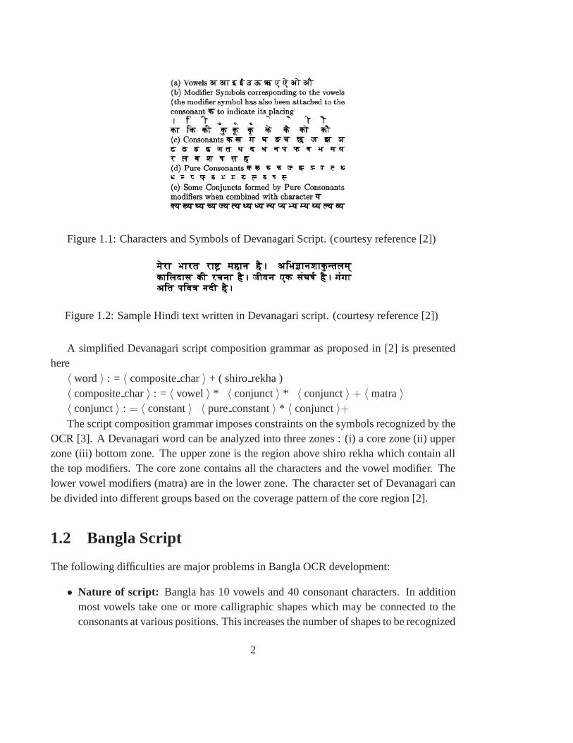
Figure 1.1: Characters and Symbols of Devanagari Script. (courtesy reference [2])
Figure 1.2: Sample Hindi text written in Devanagari script.(courtesy reference [2])
A simplified Devanagari script composition grammar as proposed in [2] is presentedhere〈 word 〉 : = 〈 compositechar〉 + ( shiro rekha )〈 compositechar〉 : = 〈 vowel 〉 * 〈 conjunct〉 * 〈 conjunct〉 + 〈matra〉〈 conjunct〉 : = 〈 constant〉 〈 pure constant〉 * 〈 conjunct〉+The script composition grammar imposes constraints on the symbols recognized by the
OCR [3]. A Devanagari word can be analyzed into three zones : (i) a core zone (ii) upperzone (iii) bottom zone. The upper zone is the region above shiro rekha which contain allthe top modifiers. The core zone contains all the characters and the vowel modifier. Thelower vowel modifiers (matra) are in the lower zone. The character set of Devanagari canbe divided into different groups based on the coverage pattern of the core region [2].
1.2 Bangla Script
The following difficulties are major problems in Bangla OCR development:
• Nature of script: Bangla has 10 vowels and 40 consonant characters. In additionmost vowels take one or more calligraphic shapes which may beconnected to theconsonants at various positions. This increases the numberof shapes to be recognized
2
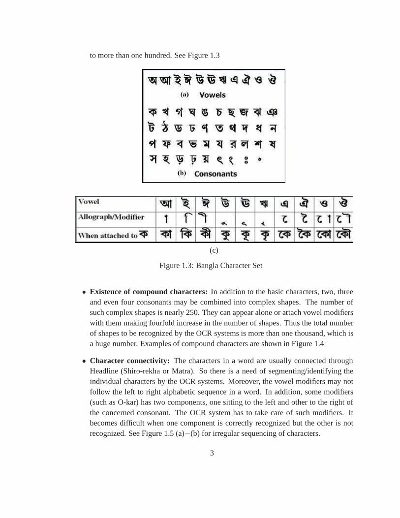
to more than one hundred. See Figure 1.3
(c)
Figure 1.3: Bangla Character Set
• Existence of compound characters:In addition to the basic characters, two, threeand even four consonants may be combined into complex shapes. The number ofsuch complex shapes is nearly 250. They can appear alone or attach vowel modifierswith them making fourfold increase in the number of shapes. Thus the total numberof shapes to be recognized by the OCR systems is more than one thousand, which isa huge number. Examples of compound characters are shown in Figure 1.4
• Character connectivity: The characters in a word are usually connected throughHeadline (Shiro-rekha or Matra). So there is a need of segmenting/identifying theindividual characters by the OCR systems. Moreover, the vowel modifiers may notfollow the left to right alphabetic sequence in a word. In addition, some modifiers(such as O-kar) has two components, one sitting to the left and other to the right ofthe concerned consonant. The OCR system has to take care of such modifiers. Itbecomes difficult when one component is correctly recognized but the other is notrecognized. See Figure 1.5 (a)−(b) for irregular sequencing of characters.
3
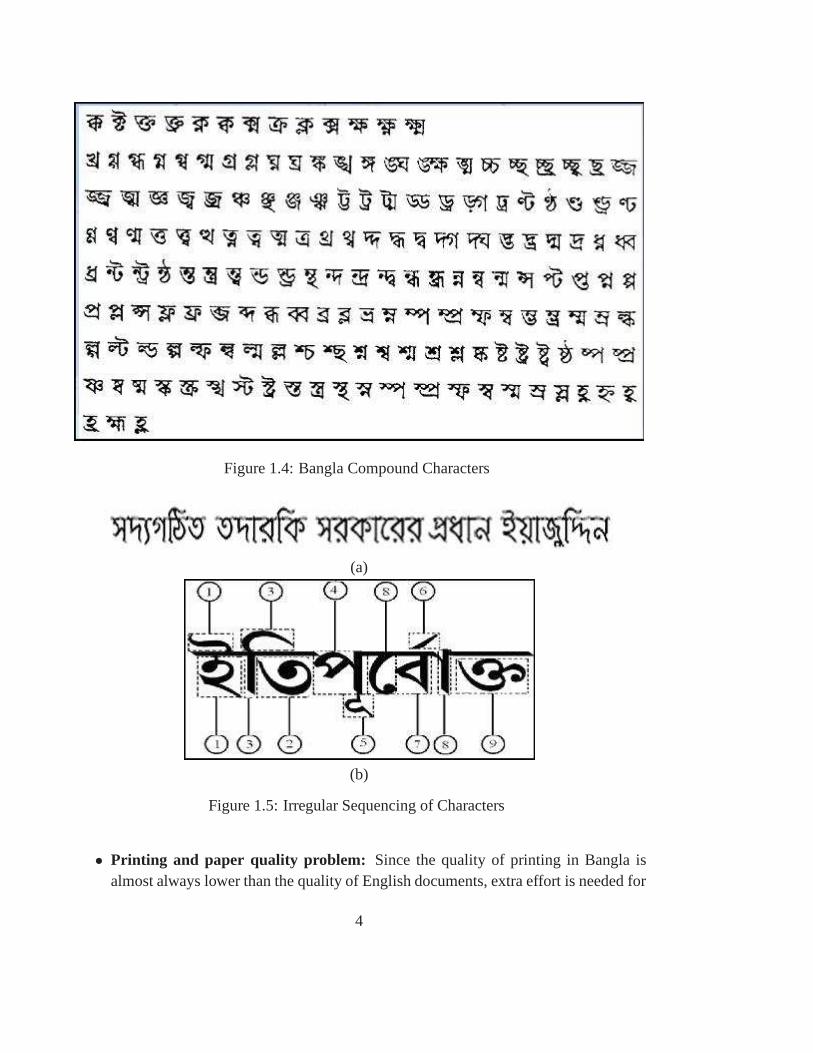
Figure 1.4: Bangla Compound Characters
(a)
(b)
Figure 1.5: Irregular Sequencing of Characters
• Printing and paper quality problem: Since the quality of printing in Bangla isalmost always lower than the quality of English documents, extra effort is needed for
4
recognition.
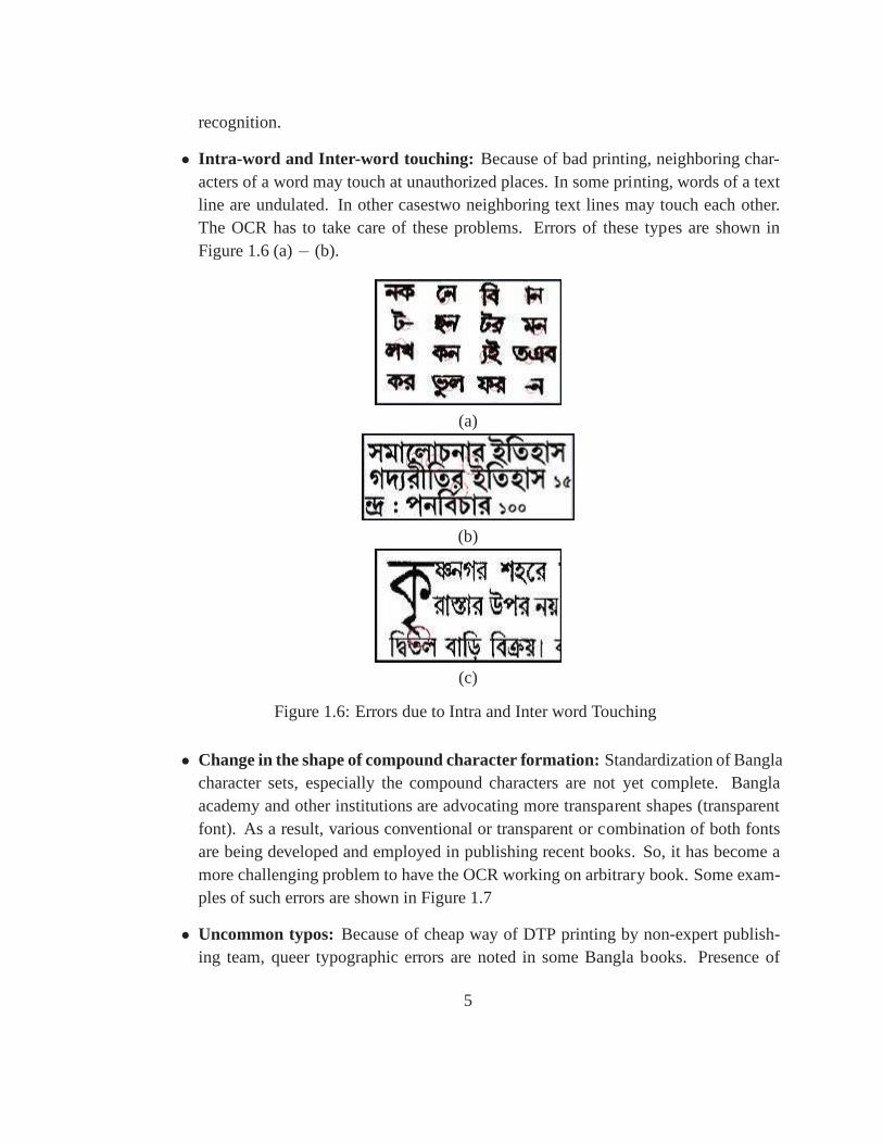
• Intra-word and Inter-word touching: Because of bad printing, neighboring char-acters of a word may touch at unauthorized places. In some printing, words of a textline are undulated. In other casestwo neighboring text lines may touch each other.The OCR has to take care of these problems. Errors of these types are shown inFigure 1.6 (a)− (b).
(a)
(b)
(c)
Figure 1.6: Errors due to Intra and Inter word Touching
• Change in the shape of compound character formation:Standardization of Banglacharacter sets, especially the compound characters are notyet complete. Banglaacademy and other institutions are advocating more transparent shapes (transparentfont). As a result, various conventional or transparent or combination of both fontsare being developed and employed in publishing recent books. So, it has become amore challenging problem to have the OCR working on arbitrary book. Some exam-ples of such errors are shown in Figure 1.7
• Uncommon typos: Because of cheap way of DTP printing by non-expert publish-ing team, queer typographic errors are noted in some Bangla books. Presence of
5
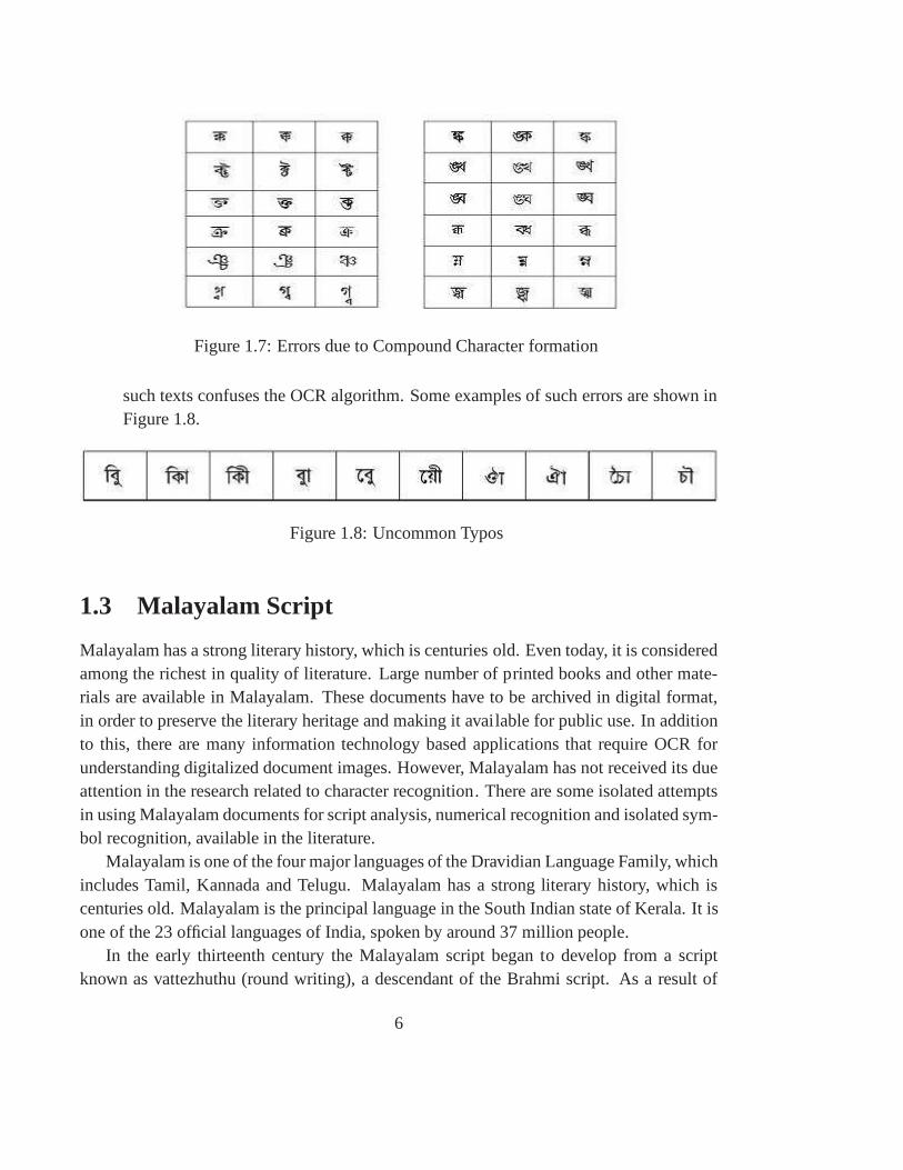
Figure 1.7: Errors due to Compound Character formation
such texts confuses the OCR algorithm. Some examples of sucherrors are shown inFigure 1.8.
Figure 1.8: Uncommon Typos
1.3 Malayalam Script
Malayalam has a strong literary history, which is centuriesold. Even today, it is consideredamong the richest in quality of literature. Large number of printed books and other mate-rials are available in Malayalam. These documents have to bearchived in digital format,in order to preserve the literary heritage and making it available for public use. In additionto this, there are many information technology based applications that require OCR forunderstanding digitalized document images. However, Malayalam has not received its dueattention in the research related to character recognition. There are some isolated attemptsin using Malayalam documents for script analysis, numerical recognition and isolated sym-bol recognition, available in the literature.
Malayalam is one of the four major languages of the DravidianLanguage Family, whichincludes Tamil, Kannada and Telugu. Malayalam has a strong literary history, which iscenturies old. Malayalam is the principal language in the South Indian state of Kerala. It isone of the 23 official languages of India, spoken by around 37 million people.
In the early thirteenth century the Malayalam script began to develop from a scriptknown as vattezhuthu (round writing), a descendant of the Brahmi script. As a result of
6
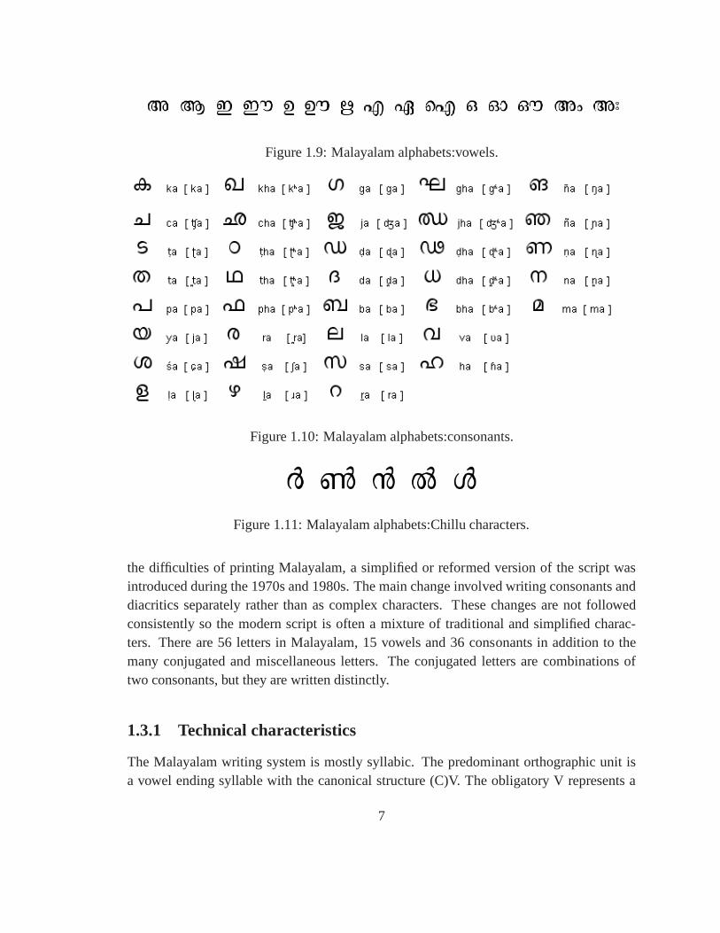
Figure 1.9: Malayalam alphabets:vowels.
Figure 1.10: Malayalam alphabets:consonants.
Figure 1.11: Malayalam alphabets:Chillu characters.
the difficulties of printing Malayalam, a simplified or reformed version of the script wasintroduced during the 1970s and 1980s. The main change involved writing consonants anddiacritics separately rather than as complex characters. These changes are not followedconsistently so the modern script is often a mixture of traditional and simplified charac-ters. There are 56 letters in Malayalam, 15 vowels and 36 consonants in addition to themany conjugated and miscellaneous letters. The conjugatedletters are combinations oftwo consonants, but they are written distinctly.
1.3.1 Technical characteristics
The Malayalam writing system is mostly syllabic. The predominant orthographic unit isa vowel ending syllable with the canonical structure (C)V. The obligatory V represents a
7
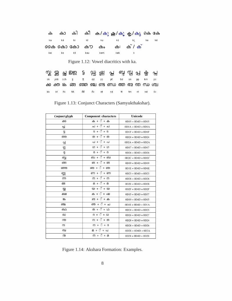
Figure 1.12: Vowel diacritics with ka.
Figure 1.13: Conjunct Characters (Samyukthakshar).
Figure 1.14: Akshara Formation: Examples.
8
short or long vowel. The optional C represents one or more consonants Except in a fewinstances the system follows the principles of phonology and mostly corresponds to thepronunciation Each consonant letter represents a single consonant sound followed by theinherent vowel /a/ thereby making an orthographic syllable. Consonant letters may also berendered as half forms which go into the constitution of consonant conjuncts. Only thosehalf forms that represent the final member of a consonant conjunct has an inherent /a/.
1.3.2 Independent vowels and Dependent vowel signs
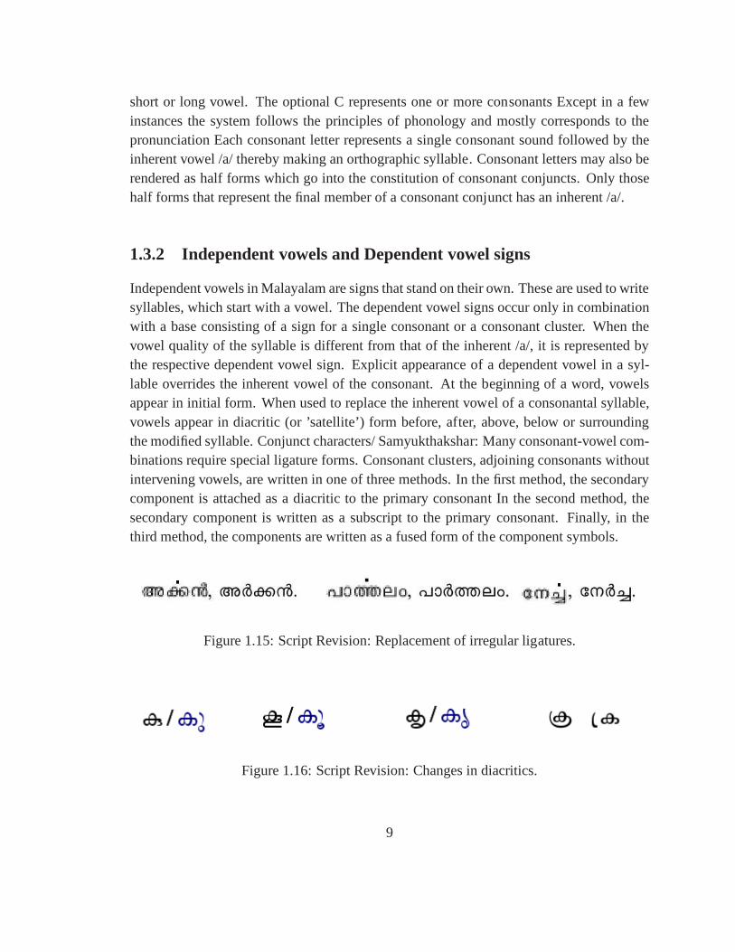
Independent vowels in Malayalam are signs that stand on their own. These are used to writesyllables, which start with a vowel. The dependent vowel signs occur only in combinationwith a base consisting of a sign for a single consonant or a consonant cluster. When thevowel quality of the syllable is different from that of the inherent /a/, it is represented bythe respective dependent vowel sign. Explicit appearance of a dependent vowel in a syl-lable overrides the inherent vowel of the consonant. At the beginning of a word, vowelsappear in initial form. When used to replace the inherent vowel of a consonantal syllable,vowels appear in diacritic (or ’satellite’) form before, after, above, below or surroundingthe modified syllable. Conjunct characters/ Samyukthakshar: Many consonant-vowel com-binations require special ligature forms. Consonant clusters, adjoining consonants withoutintervening vowels, are written in one of three methods. In the first method, the secondarycomponent is attached as a diacritic to the primary consonant In the second method, thesecondary component is written as a subscript to the primaryconsonant. Finally, in thethird method, the components are written as a fused form of the component symbols.
Figure 1.15: Script Revision: Replacement of irregular ligatures.
Figure 1.16: Script Revision: Changes in diacritics.
9
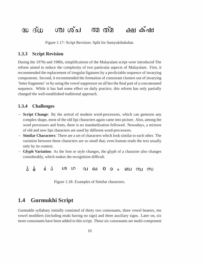
Figure 1.17: Script Revision: Split for Samyukthakshar.
1.3.3 Script Revision
During the 1970s and 1980s, simplifications of the Malayalamscript were introduced Thereform aimed to reduce the complexity of two particular aspects of Malayalam. First, itrecommended the replacement of irregular ligatures by a predictable sequence of invaryingcomponents. Second, it recommended the formation of consonant clusters out of invarying’letter fragments’ or by using the vowel suppressor on all but the final part of a concatenatedsequence. While it has had some effect on daily practice, this reform has only partiallychanged the well-established traditional approach.
1.3.4 Challenges
− Script Change: By the arrival of modern word-processors, which can generate anycomplex shape, most of the old lipi characters again came into picture. Also, among theword processors and fonts, there is no standardization followed. Nowadays, a mixtureof old and new lipi characters are used by different word-processors.
− Similar Characters: There are a set of characters which look similar to each other. Thevariation between these characters are so small that, even human reads the text usuallyonly by its context.
− Glyph Variation : As the font or style changes, the glyph of a character also changesconsiderably, which makes the recognition difficult.
Figure 1.18: Examples of Similar characters.
1.4 Gurmukhi Script
Gurmukhi syllabary initially consisted of thirty two consonants, three vowel bearers, tenvowel modifiers (including mukt having no sign) and three auxiliary signs. Later on, sixmore consonants have been added to this script. These six consonants are multi-component
10
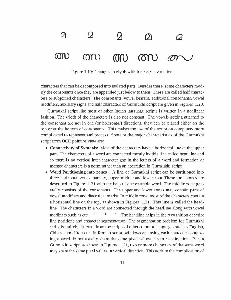
Figure 1.19: Changes in glyph with font/ Style variation.
characters that can be decomposed into isolated parts. Besides these, some characters mod-ify the consonants once they are appended just below to them.These are called half charac-ters or subjoined characters. The consonants, vowel bearers, additional consonants, vowelmodifiers, auxiliary signs and half characters of Gurmukhi script are given in Figures 1.20.
Gurmukhi script like most of other Indian language scripts is written in a nonlinearfashion. The width of the characters is also not constant. The vowels getting attached tothe consonant are not in one (or horizontal) directions, they can be placed either on thetop or at the bottom of consonants. This makes the use of the script on computers morecomplicated to represent and process. Some of the major characteristics of the Gurmukhiscript from OCR point of view are:
• Connectivity of Symbols: Most of the characters have a horizontal line at the upperpart. The characters of a word are connected mostly by this line called head line andso there is no vertical inter-character gap in the letters ofa word and formation ofmerged characters is a norm rather than an aberration in Gurmukhi script.• Word Partitioning into zones : A line of Gurmukhi script can be partitioned into
three horizontal zones, namely, upper, middle and lower zone.These three zones aredescribed in Figure 1.21 with the help of one example word. The middle zone gen-erally consists of the consonants. The upper and lower zonesmay contain parts ofvowel modifiers and diacritical marks. In middle zone, most of the characters containa horizontal line on the top, as shown in Figures 1.21. This line is called the head-line. The characters in a word are connected through the headline along with vowel
modifiers such as etc. The headline helps in the recognition of scriptline positions and character segmentation. The segmentation problem for Gurmukhiscript is entirely different from the scripts of other common languages such as English,Chinese and Urdu etc. In Roman script, windows enclosing each character compos-ing a word do not usually share the same pixel values in vertical direction. But inGurmukhi script, as shown in Figures 1.21, two or more characters of the same wordmay share the same pixel values in vertical direction. This adds to the complication of
11
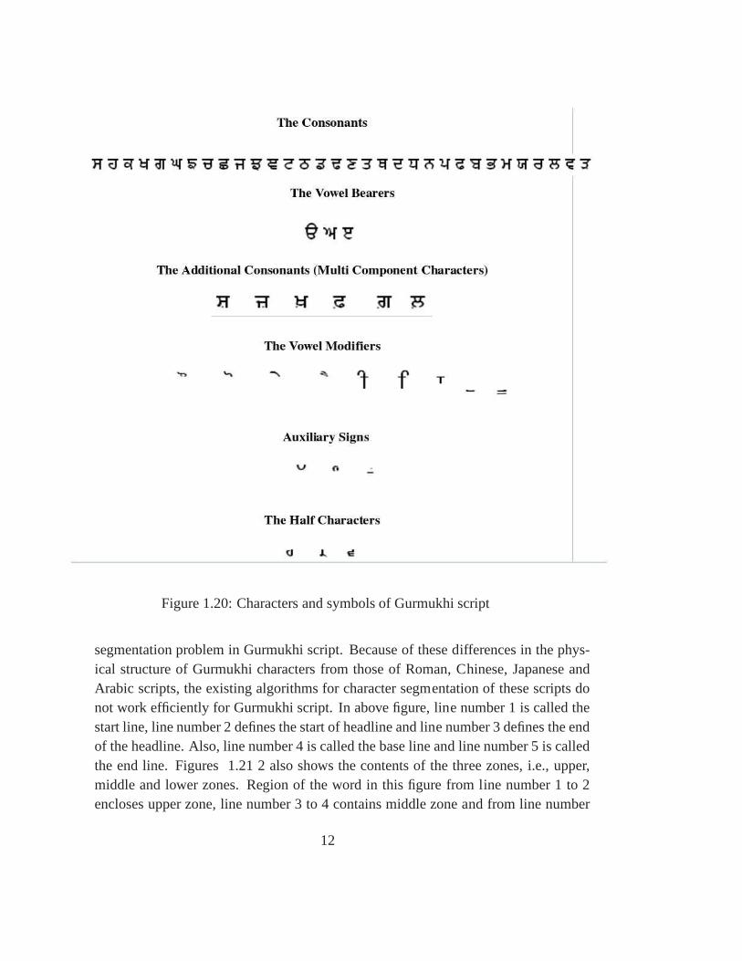
Figure 1.20: Characters and symbols of Gurmukhi script
segmentation problem in Gurmukhi script. Because of these differences in the phys-ical structure of Gurmukhi characters from those of Roman, Chinese, Japanese andArabic scripts, the existing algorithms for character segmentation of these scripts donot work efficiently for Gurmukhi script. In above figure, line number 1 is called thestart line, line number 2 defines the start of headline and line number 3 defines the endof the headline. Also, line number 4 is called the base line and line number 5 is calledthe end line. Figures 1.21 2 also shows the contents of the three zones, i.e., upper,middle and lower zones. Region of the word in this figure from line number 1 to 2encloses upper zone, line number 3 to 4 contains middle zone and from line number
12
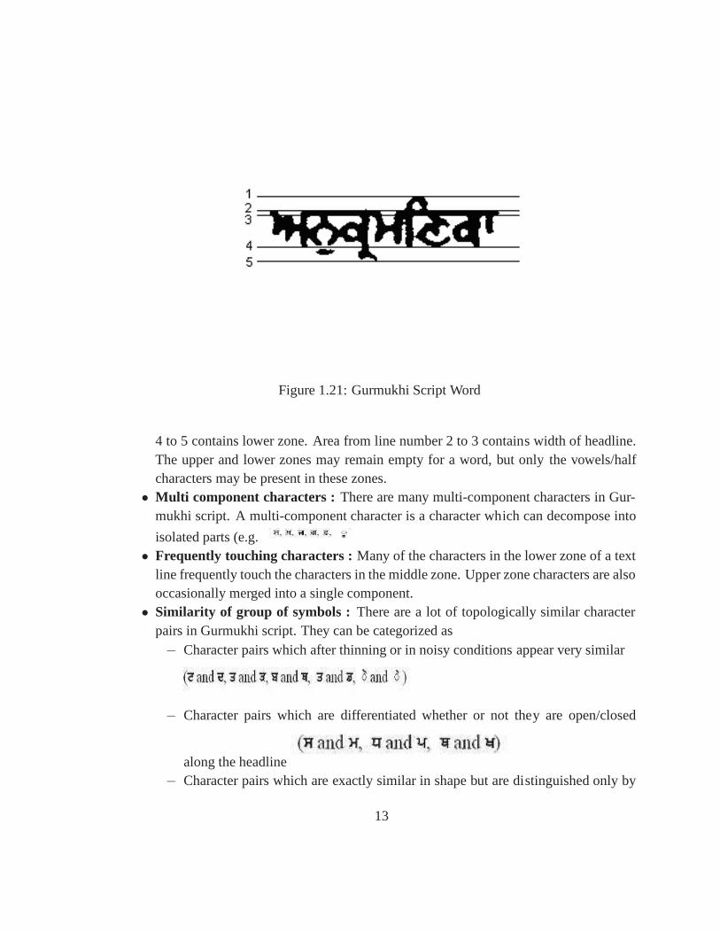
Figure 1.21: Gurmukhi Script Word
4 to 5 contains lower zone. Area from line number 2 to 3 contains width of headline.The upper and lower zones may remain empty for a word, but onlythe vowels/halfcharacters may be present in these zones.• Multi component characters : There are many multi-component characters in Gur-
mukhi script. A multi-component character is a character which can decompose into
isolated parts (e.g.• Frequently touching characters :Many of the characters in the lower zone of a text
line frequently touch the characters in the middle zone. Upper zone characters are alsooccasionally merged into a single component.• Similarity of group of symbols : There are a lot of topologically similar character
pairs in Gurmukhi script. They can be categorized as− Character pairs which after thinning or in noisy conditionsappear very similar
− Character pairs which are differentiated whether or not they are open/closed
along the headline− Character pairs which are exactly similar in shape but are distinguished only by
13
the presence/absence of a dot in the feet of a character.
1.4.1 Challenges in Developing Gurmukhi OCR
Touching Characters
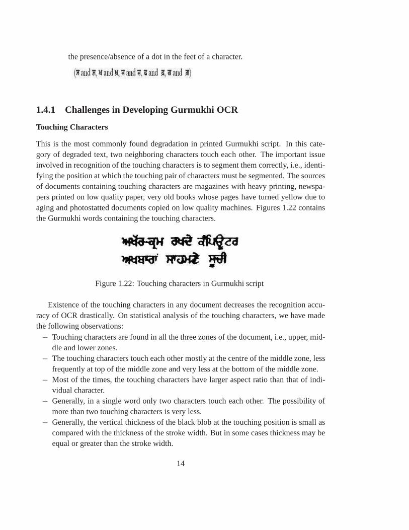
This is the most commonly found degradation in printed Gurmukhi script. In this cate-gory of degraded text, two neighboring characters touch each other. The important issueinvolved in recognition of the touching characters is to segment them correctly, i.e., identi-fying the position at which the touching pair of characters must be segmented. The sourcesof documents containing touching characters are magazineswith heavy printing, newspa-pers printed on low quality paper, very old books whose pageshave turned yellow due toaging and photostatted documents copied on low quality machines. Figures 1.22 containsthe Gurmukhi words containing the touching characters.
Figure 1.22: Touching characters in Gurmukhi script
Existence of the touching characters in any document decreases the recognition accu-racy of OCR drastically. On statistical analysis of the touching characters, we have madethe following observations:− Touching characters are found in all the three zones of the document, i.e., upper, mid-
dle and lower zones.− The touching characters touch each other mostly at the centre of the middle zone, less
frequently at top of the middle zone and very less at the bottom of the middle zone.− Most of the times, the touching characters have larger aspect ratio than that of indi-
vidual character.− Generally, in a single word only two characters touch each other. The possibility of
more than two touching characters is very less.− Generally, the vertical thickness of the black blob at the touching position is small as
compared with the thickness of the stroke width. But in some cases thickness may beequal or greater than the stroke width.
14
− Generally, the characters of Indian scripts contain sidebars at their right end, e.g., inGurmukhi script 12 consonants have side bars at their right end. The possibility oftouching is very high at this position.
Segmentation of the touching characters is a challenging task. There are two key issuesinvolved in this problem. The first issue is to find the candidate of segmentation, i.e., tofind the segment of the complete word which may contain the touching characters. Secondissue is to find the break location within the candidate of segmentation, i.e., to find thecolumn which will correctly segment the two touching characters into isolated characters.The problem of segmenting the touching characters in Gurmukhi script is quite differentfrom the Roman script in many aspects:• In Gurmukhi script the touching characters can be found in upper, middle and lower
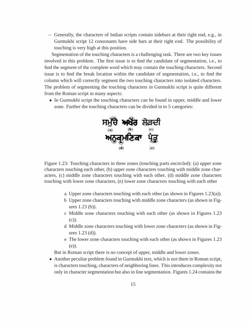
zone. Further the touching characters can be divided in to 5 categories:
Figure 1.23: Touching characters in three zones (touching parts encircled): (a) upper zonecharacters touching each other, (b) upper zone characters touching with middle zone char-acters, (c) middle zone characters touching with each other, (d) middle zone characterstouching with lower zone characters, (e) lower zone characters touching with each other
a Upper zone characters touching with each other (as shown inFigures 1.23(a)).b Upper zone characters touching with middle zone characters (as shown in Fig-
ures 1.23 (b)).c Middle zone characters touching with each other (as shown in Figures 1.23
(c)).d Middle zone characters touching with lower zone characters (as shown in Fig-
ures 1.23 (d)).e The lower zone characters touching with each other (as shown in Figures 1.23
(e)).But in Roman script there is no concept of upper, middle and lower zones.• Another peculiar problem found in Gurmukhi text, which is not there in Roman script,
is characters touching, characters of neighboring lines. This introduces complexity notonly in character segmentation but also in line segmentation. Figures 1.24 contains the
15
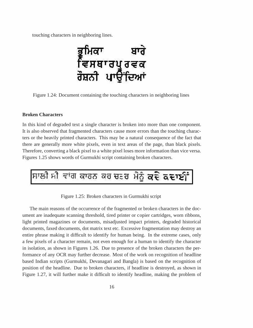
touching characters in neighboring lines.
Figure 1.24: Document containing the touching characters in neighboring lines
Broken Characters
In this kind of degraded text a single character is broken into more than one component.It is also observed that fragmented characters cause more errors than the touching charac-ters or the heavily printed characters. This may be a naturalconsequence of the fact thatthere are generally more white pixels, even in text areas of the page, than black pixels.Therefore, converting a black pixel to a white pixel loses more information than vice versa.Figures 1.25 shows words of Gurmukhi script containing broken characters.
Figure 1.25: Broken characters in Gurmukhi script
The main reasons of the occurrence of the fragmented or broken characters in the doc-ument are inadequate scanning threshold, tired printer or copier cartridges, worn ribbons,light printed magazines or documents, misadjusted impact printers, degraded historicaldocuments, faxed documents, dot matrix text etc. Excessivefragmentation may destroy anentire phrase making it difficult to identify for human being. In the extreme cases, onlya few pixels of a character remain, not even enough for a humanto identify the characterin isolation, as shown in Figures 1.26. Due to presence of thebroken characters the per-formance of any OCR may further decrease. Most of the work on recognition of headlinebased Indian scripts (Gurmukhi, Devanagari and Bangla) is based on the recognition ofposition of the headline. Due to broken characters, if headline is destroyed, as shown inFigure 1.27, it will further make it difficult to identify headline, making the problem of
16
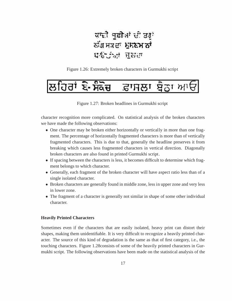
Figure 1.26: Extremely broken characters in Gurmukhi script
Figure 1.27: Broken headlines in Gurmukhi script
character recognition more complicated. On statistical analysis of the broken characterswe have made the following observations:
• One character may be broken either horizontally or vertically in more than one frag-ment. The percentage of horizontally fragmented characters is more than of verticallyfragmented characters. This is due to that, generally the headline preserves it frombreaking which causes less fragmented characters in vertical direction. Diagonallybroken characters are also found in printed Gurmukhi script.• If spacing between the characters is less, it becomes difficult to determine which frag-
ment belongs to which character.• Generally, each fragment of the broken character will have aspect ratio less than of a
single isolated character.• Broken characters are generally found in middle zone, less in upper zone and very less
in lower zone.• The fragment of a character is generally not similar in shapeof some other individual
character.
Heavily Printed Characters
Sometimes even if the characters that are easily isolated, heavy print can distort theirshapes, making them unidentifiable. It is very difficult to recognize a heavily printed char-acter. The source of this kind of degradation is the same as that of first category, i.e., thetouching characters. Figure 1.28consists of some of the heavily printed characters in Gur-mukhi script. The following observations have been made on the statistical analysis of the
17

Figure 1.28: Heavily printed characters in Gurmukhi script
heavily printed Gurmukhi characters:
• The aspect ratio of the heavily printed characters is almostsame as that of the originalcharacter.• It is very difficult to extract the features of the heavily printed character, as it is just
like a blob of black pixels of the height and width of the original character, with noascenders or descenders to help distinguish them.• Generally, the heavily printed characters are also touching with neighboring charac-
ters, i.e., also falling in touching character category.• Most of the characters, which are heavily printed have loop in their structure.• Heavily printed characters can be found in middle zone as well as lower and upper
zone also. Even in clean documents, characters in lower and upper zone are heavilyprinted.• Most of the times, the shape of a heavily printed character may look like some other
character.
Since the reasons of production of heavily printed characters are same as that of touchingcharacters, most of time the problem of heavily printed characters is considered along withthe problem of touching characters. Leading OCR of Roman script fails to recognize theheavily printed characters. Nothing specific has been done until now in Indian scripts todeal with the problem of heavily printed characters. No special work has been reportedfor solving the problem of heavily printed characters. The best solution to recognize heav-ily printed characters is to bypass the recognition processuntil post-processing stage isencountered. Here on the basis of dictionary look up if the word containing the heavilyprinted characters is not a valid word, the dictionary look up post-processing process workwill correct it automatically.
Multiple Skewness in documents
Another typical problem found in old printed Gurmukhi text is existence of multiple skew-ness on same page. Each word or line could be skewed differently, which calls for develop-ment of skew detection and correction algorithms at global and local level. As an example,
18
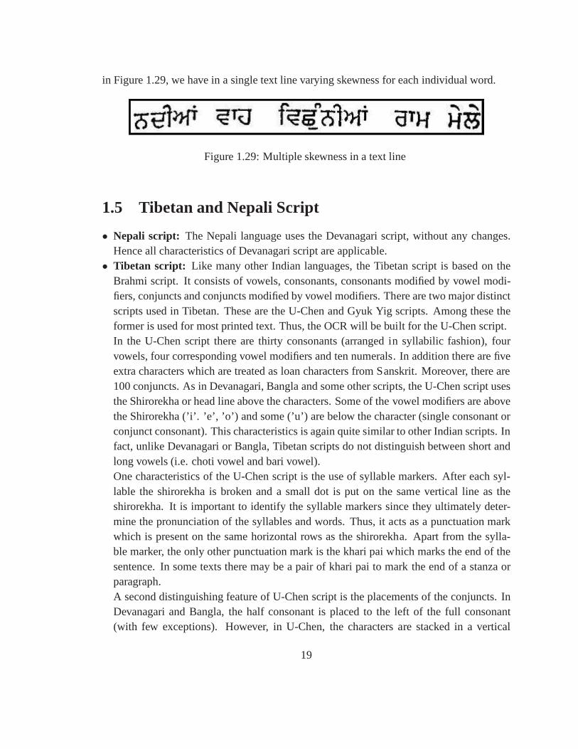
in Figure 1.29, we have in a single text line varying skewnessfor each individual word.
Figure 1.29: Multiple skewness in a text line
1.5 Tibetan and Nepali Script
• Nepali script: The Nepali language uses the Devanagari script, without anychanges.Hence all characteristics of Devanagari script are applicable.• Tibetan script: Like many other Indian languages, the Tibetan script is based on the
Brahmi script. It consists of vowels, consonants, consonants modified by vowel modi-fiers, conjuncts and conjuncts modified by vowel modifiers. There are two major distinctscripts used in Tibetan. These are the U-Chen and Gyuk Yig scripts. Among these theformer is used for most printed text. Thus, the OCR will be built for the U-Chen script.In the U-Chen script there are thirty consonants (arranged in syllabilic fashion), fourvowels, four corresponding vowel modifiers and ten numerals. In addition there are fiveextra characters which are treated as loan characters from Sanskrit. Moreover, there are100 conjuncts. As in Devanagari, Bangla and some other scripts, the U-Chen script usesthe Shirorekha or head line above the characters. Some of thevowel modifiers are abovethe Shirorekha (’i’. ’e’, ’o’) and some (’u’) are below the character (single consonant orconjunct consonant). This characteristics is again quite similar to other Indian scripts. Infact, unlike Devanagari or Bangla, Tibetan scripts do not distinguish between short andlong vowels (i.e. choti vowel and bari vowel).One characteristics of the U-Chen script is the use of syllable markers. After each syl-lable the shirorekha is broken and a small dot is put on the same vertical line as theshirorekha. It is important to identify the syllable markers since they ultimately deter-mine the pronunciation of the syllables and words. Thus, it acts as a punctuation markwhich is present on the same horizontal rows as the shirorekha. Apart from the sylla-ble marker, the only other punctuation mark is the khari pai which marks the end of thesentence. In some texts there may be a pair of khari pai to markthe end of a stanza orparagraph.A second distinguishing feature of U-Chen script is the placements of the conjuncts. InDevanagari and Bangla, the half consonant is placed to the left of the full consonant(with few exceptions). However, in U-Chen, the characters are stacked in a vertical
19
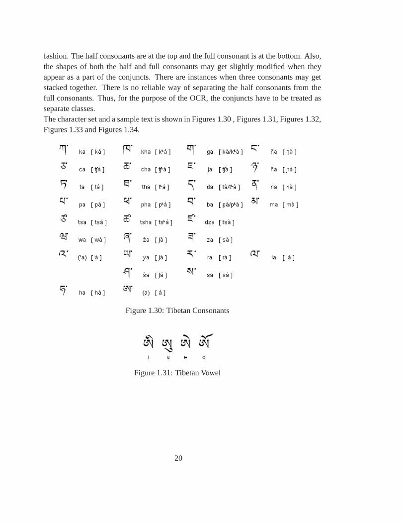
fashion. The half consonants are at the top and the full consonant is at the bottom. Also,the shapes of both the half and full consonants may get slightly modified when theyappear as a part of the conjuncts. There are instances when three consonants may getstacked together. There is no reliable way of separating thehalf consonants from thefull consonants. Thus, for the purpose of the OCR, the conjuncts have to be treated asseparate classes.The character set and a sample text is shown in Figures 1.30 , Figures 1.31, Figures 1.32,Figures 1.33 and Figures 1.34.
Figure 1.30: Tibetan Consonants
Figure 1.31: Tibetan Vowel
20
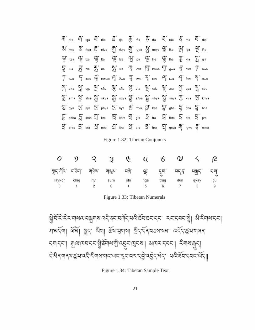
Figure 1.32: Tibetan Conjuncts
Figure 1.33: Tibetan Numerals
Figure 1.34: Tibetan Sample Text
21

1.6 Oriya Script
Oriya is one of the scheduled languages of India. It is the principal language of communica-tion in the state of Orissa, spoken by over 23 million people comprising 84% of population(1991 Census). It is the official language of the state. Oriyabelongs to the Eastern groupof Indo-Aryan language family and has evolved around 10th century AD. It is the southernmost Indo-Aryan language placed at the boundary of Dravidian family of languages alongwith some Munda group of languages belonging to Austro-Asiatic family of languages.Oriya language has a rich literary history. A large number ofprinted books and other mate-rials are available in Oriya . For the preservation of these invaluable literary heritages andto make them available for public use these documents are to be archived in digital format.For that and for many IT based applications we need an OCR System for understandingdigitized document images. Oriya script in stone engravings, copper plates, and palm-leafmanuscripts shows its antiquity. It has been a carrier of vibrant literature, a medium ofinstruction and a means of communication through the centuries. Modern Oriya script, likeDevanagari script is a descendant of Brahmi script. But unlike Devanagari the charactershave got a circular look, possibly under influence of Dravidian writing system and to avoidhorizontal lines to be drawn on palm-leaves used as writing material in the earlier times.Oriya writing system is mostly syllabic, the effective unitbeing an orthographic syllableconsisting of a vowel (V) only or a consonant and vowel (CV) core and optionally one ormore preceding consonants , with canonical structure of (C)(C)(C)CV . The orthographicsyllable need not correspond exactly with a phonological syllable, especially when a con-sonant cluster is involved, but the writing system is built on phonological principles andtends to correspond quite closely to pronunciation.
Oriya script consists of simple and complex characters. There are 13 vowels, 3 vowelmodifiers, 37 simple consonants, 10 numerical digits and more than 59 composite charac-ters (juktas) in Oriya alphabets.
One of the major characteristics of Oriya elementary characters is that most their upperone third is circular and a subset of them have a vertical straight line at their rightmost part.The conjuncts have quite complex shapes. The matras are comparatively small in size. Inwriting a text document all elementary characters and some matras fall along a base line.Different matras take relative positions with consonant characters like before or after them,or upper or lower to the base line, and sometimes at the upper-right or lower-right corners.The matras sometimes get touched with common characters, and more than one modifiercombined forming a composite modifier.
22

1.7 Kannada Script
Kannada along with other Indian language scripts shares a large number of structural fea-tures. The writing system of Kannada script encompasses theprinciples governing thephonetics and a syllabic writing systems, and phonemic writing systems (alphabets). Theeffective unit of writing Kannada is the orthographic syllable consisting of a consonant andvowel (CV) core and optionally, one or more preceding consonants, with a canonical struc-ture of ((C) C) CV. The orthographic syllable need not correspond exactly with a phonolog-ical syllable, especially when a consonant cluster is involved, but the writing system is builton phonological principles and tends to correspond quite closely to pronunciation. The or-thographic syllable is built up of alphabetic pieces, the actual letters of Kannada script.These consist of distinct character types: Consonant letters, independent vowels and thecorresponding dependent vowel signs. In a text sequence, these characters are stored inlogical phonetic order. Most of the characters in script arecircular in nature. Most of thecharacters by nature are separated, with top part and consonant conjunct. Problem arises ifthe character is broken into components and their separations are above the separation ofconsonant and consonant conjunct. In case of joint character, we have thought of an ideato separate them using the concept of tangents. Since characters are circular in nature, andthe point they touch each other can be found. Also using Graphbased approach, we can dosub-matrix matching. Modern kannada script has 48 characters, called varnamale. Thesealphabets broadly characterized in two categories, vowelsand consonants, Consonants aredivided into grouped consonants and ungrouped consonants.There are 14 vowels 34 con-sonants and 10 numerals. Vowels along with consonants constitute basic character. Vowelmodifiers can appear to the right on the top or at the bottom of abase consonant.
1.8 Gujarati Script
Gujarati script was adapted from the Devanagari script to write the Gujarati language spo-ken by about 50 million people in the western part of India. The earliest known documentin the Gujarati script is a manuscript dating from 1592, and the script first appeared inprint in a 1797 advertisement. Until the 19th century it was used mainly for writing lettersand keeping accounts, while the Devanagari script was used for literature and academicwritings [4].
Apart from state of Gujarat in India, Gujarati speakers are spread across all parts ofIndia and Gujarati Diaspora is very large. The importance ofGujarati script and languagecan be estimated by the fact that almost all work of M. K. Gandhi was originally in Gujarati.It may also be noted that oldest continuously published newspaper in India is a Gujarati
23

daily Mumbai Samachar, published since 1822 (first by Fardoonjee Marzban).
Figure 1.35: Table for Gujarati Script
Gujarati has 11 vowels and 34+21 consonants. Apart from these basic symbols, othersymbols called vowel modifiers are used to denote the attachment of vowels with the coreconsonants. Consonant-Vowel combinations occur very often in most of the Indic lan-guages including Gujarati. This is denoted by attaching a symbol, unique for each vowel,to the consonant, called a Dependent Vowel Modifier or Matra.The matra can appear be-fore, after, above or below the core consonant. In addition to basic consonants, like mostIndic scripts, Gujarati also uses consonant clusters (conjuncts). That is, consonants withoutthe inherent vowel sound are combined and there by leading tothree possibilities for theshape of the resulting conjuncts :
1. Conjunct shape is derived by connecting a part of preceding consonant of the follow-ing one
2. The conjunct take completely different shape
3. Addition of some mark indicating conjunct formation in upper/middle/lower zone(mainly conjuncts involving /r/).
Moreover, conjuncts may themselves occur in half forms. Table 1.35 also lists some ex-amples of conjuncts. Reference [5] gives detailed description on Gujarati script with the
1Two conjuncts /ksha/ and /jya/ are treated as if they are basic consonants in Gujarati script
24

rules to form conjuncts and other modifications that might take place in the shapes of basicconsonant symbols. Table 1.35 gives examples of Gujarati consonants,
It can be seen from Table 1.35 above that the shapes of many Gujarati characters aresimilar to those of the phonetically corresponding characters of Devanagari script. As inthe case of other Indic scripts, Gujarati also does not have the distinction of Lower andUpper Cases. In spite of these similarities with the Devanagari script, Gujarati script hasmany distinct characteristics such as the absence of the so-called shirorekha (header line)in the script and differences in the shapes of many of the consonants and vowels etc.
Similar to the text written in Devanagari or Bangla script, text in Gujarati script can alsobe divided into three logical zones : Upper, Middle and Loweras shown in Figure 1.36.
Figure 1.36: Logical Zones
Gujarati, due to its peculiar characteristics needs to be treated differently from the otherIndo-Aryan scripts like Devanagari, Bangla, Gurmukhi etc.Unlike, many Indian scriptslike Bangla, Devanagari the development of OCR technology has not been explored much.many So far. The first published work on recognizing a limitedset of Gujarati charactersis that of Samir Antani et. al. and that too as late as in 1999. The recognition accuracyreported was very poor and not at all acceptable and there were no published work onGujarati document image analysis till 2005. Subsequently there has been a few efforts forGujarati Character recognition using modern techniques like wavelets as feature extractorand different artificial neural network architectures as classifiers [6][7][8].
There are several challenging issues in Gujarati Characterrecognition viz. :
1. Similar looking glyphs : e.g.. /ka/ /da/ /tha/ , /gha/ /dha/ /dya/ , later half of /la/ and/na/
2. almost same shapes for : alphabet /pa/ and numeral 5
3. More than one way in which basic glyphs of an akshara combine. e.g. /la/ /ha/
4. Non uniform behavior of vowel modifiers.
5. Touching and broken characters
6. Accurate identification of zone boundary absence of shirorekha
25

1.9 Telugu Script
1.9.1 Script Characteristics
Telugu is a phonetic language, written from left to right, with each character representinga syllable. Telugu is one of the most complex scripts with highly curved letters that havepractically no linear strokes which characterize English and many north Indian scripts in-cluding Devanagari. The Telugu alphabet consists of 52 letters with 14 vowels, two vowelmodifiers and 36 consonants. One of the 14 vowels is not used inany texts, even those dat-ing back a few centuries, and is not shown in Figure 1.37. Another vowel, the seventh fromthe left in Figure 1.37(a) is no longer in use but occurs in several written texts produceduntil a few years ago. The two vowel modifiers are shown at the end of the list of vowels.
(a)
(b)
Figure 1.37: The basic Telugu alphabet: (a) vowels, (b) consonants
In addition, several semi-vowels and consonant modifiers are used for creatingaksharasrepresenting complex syllables. These additional orthographic units are shown in Figure1.38.
The vowels, consonants, semi-vowels and consonant modifiers together provide roughly100 basic orthographic units that are combined together in different ways to represent allthe frequently used syllables (estimated between 5000 and 10000) in the language.
Differences from English text are strikingly apparent in the composition of variouscharacters. While written words and sentences are linear left-to-right, the semi-vowels andconsonant-modifiers are placed above and below the basic consonants. In Figure 1.39,the first two characters are examples of a pure vowel (’a’ sound) and a basic consonant
26
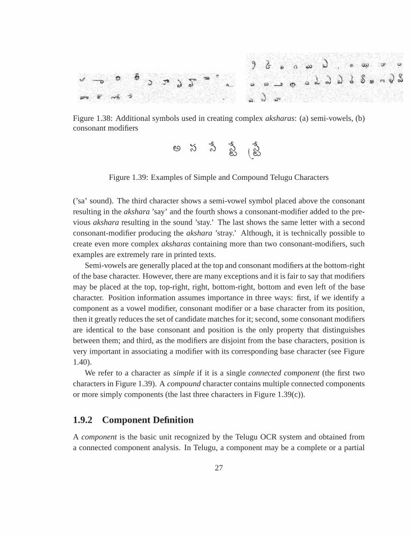
Figure 1.38: Additional symbols used in creating complexaksharas: (a) semi-vowels, (b)consonant modifiers
Figure 1.39: Examples of Simple and Compound Telugu Characters
(’sa’ sound). The third character shows a semi-vowel symbolplaced above the consonantresulting in theakshara’say’ and the fourth shows a consonant-modifier added to the pre-viousakshararesulting in the sound ’stay.’ The last shows the same letterwith a secondconsonant-modifier producing theakshara’stray.’ Although, it is technically possible tocreate even more complexaksharascontaining more than two consonant-modifiers, suchexamples are extremely rare in printed texts.
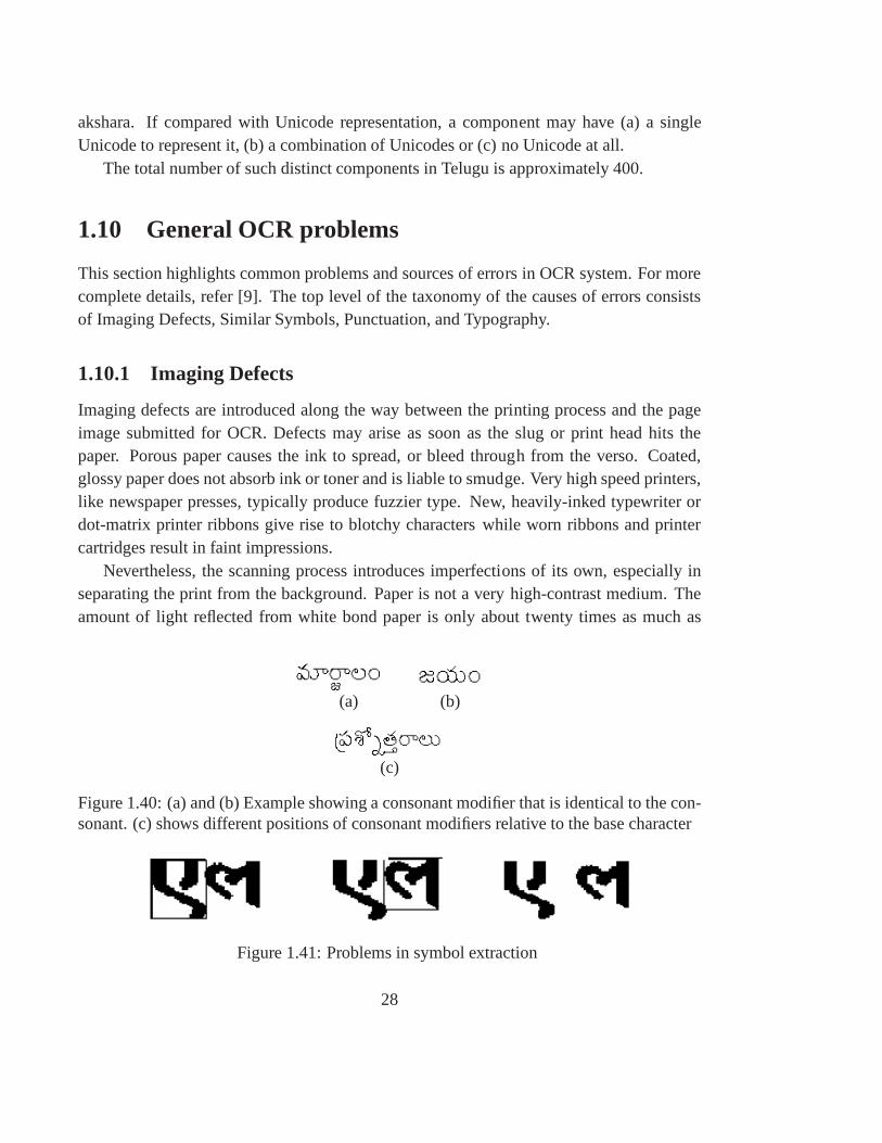
Semi-vowels are generally placed at the top and consonant modifiers at the bottom-rightof the base character. However, there are many exceptions and it is fair to say that modifiersmay be placed at the top, top-right, right, bottom-right, bottom and even left of the basecharacter. Position information assumes importance in three ways: first, if we identify acomponent as a vowel modifier, consonant modifier or a base character from its position,then it greatly reduces the set of candidate matches for it; second, some consonant modifiersare identical to the base consonant and position is the only property that distinguishesbetween them; and third, as the modifiers are disjoint from the base characters, position isvery important in associating a modifier with its corresponding base character (see Figure1.40).
We refer to a character assimpleif it is a singleconnected component(the first twocharacters in Figure 1.39). Acompoundcharacter contains multiple connected componentsor more simply components (the last three characters in Figure 1.39(c)).
1.9.2 Component Definition
A componentis the basic unit recognized by the Telugu OCR system and obtained froma connected component analysis. In Telugu, a component may be a complete or a partial
27
akshara. If compared with Unicode representation, a component may have (a) a singleUnicode to represent it, (b) a combination of Unicodes or (c)no Unicode at all.
The total number of such distinct components in Telugu is approximately 400.
1.10 General OCR problems
This section highlights common problems and sources of errors in OCR system. For morecomplete details, refer [9]. The top level of the taxonomy ofthe causes of errors consistsof Imaging Defects, Similar Symbols, Punctuation, and Typography.
1.10.1 Imaging Defects
Imaging defects are introduced along the way between the printing process and the pageimage submitted for OCR. Defects may arise as soon as the slugor print head hits thepaper. Porous paper causes the ink to spread, or bleed through from the verso. Coated,glossy paper does not absorb ink or toner and is liable to smudge. Very high speed printers,like newspaper presses, typically produce fuzzier type. New, heavily-inked typewriter ordot-matrix printer ribbons give rise to blotchy characterswhile worn ribbons and printercartridges result in faint impressions.
Nevertheless, the scanning process introduces imperfections of its own, especially inseparating the print from the background. Paper is not a veryhigh-contrast medium. Theamount of light reflected from white bond paper is only about twenty times as much as
(a) (b)
(c)
Figure 1.40: (a) and (b) Example showing a consonant modifierthat is identical to the con-sonant. (c) shows different positions of consonant modifiers relative to the base character
Figure 1.41: Problems in symbol extraction
28
that from solid, dark type. With high-contrast film, ratios of several hundred to one areachievable: that is why film is used as the master image in high-quality typesetters. Scan-ners are much more vulnerable than human readers to low contrast and to variations in theforeground and background reflectance of the page. Many OCR systems can adjust thescanner threshold on the basis of a preliminary scan of the page, and some can even setdifferent values for parts of the page. On high-contrast pages (and all printing and copyingprocesses intended for text are designed to produce high-contrast), the choice of thresholdis not critical.
The page is usually sampled both horizontally and vertically at the rate of 240 or 300dots per inch (dpi). The trend is towards higher sampling rates, and some OCR packagescan take advantage of 400 dpi or 600 dpi images. Others merelysubsample or interpolatethe image to 300 dpi. Hairline strokes and small openings aremuch less likely to be de-tected in text set in a small point size (6-pt or 8-pt) than in “normal” (10-12 pt) sizes. (Ifthe threshold is set low enough to detect hairline strokes, then small white openings will befilled.) Most OCR systems also accept facsimile images in coarse or fine mode.
1.10.2 Similar Symbols
The study of invariant features that describe printed and hand-printed characters remains atopic of continuing interest. However, almost any attempt at verbal or formal mathematicaldefinition of the shape of any particular letter will occasionally fail: there will be imagesthat obey the description that will be instantly recognizable as belonging to another class,and images that do not obey the description that would be correctly classified by any human.An instructive illustration showing how any of the ten numerals can be deformed into anyof the others through a series of continuous transformations is found in G.G.N. Wright’s1952 The Writing of Arabic Numerals (University of London Press).
A more subtle aspect of shape is the graphic unity of all of thealphabetic charactersof a given typeface. Type designers strive to achieve such unity yet give their typeface adistinctive personality suitable for a particular context. Among the shape features used todistinguish typefaces are the aspect-ratios of the characters, the lengths of the ascendersand descenders, the ratios of the widths of horizontal, vertical and slanted strokes (which,even in a given typeface, must be altered slightly from point-size to point-size to preservethe illusion of sameness), the size and form of serifs, the eccentricity of ovals, the flare ofhooks, and so forth.
The confusion between similar shapes in contemporary printed text is easily resolvedby human readers, because they don’t consider each letter ornumeral in isolation. In ad-dition to drawing on context, experienced readers adapt instantly to each typeface. Type
29
designers carefully preserving the distinction between different symbols in the same type-face. It is therefore far more likely for a symbol to resemblea different symbol in anothertypeface than one in its own typeface. We expect that more andmore of these clues, whichgo well beyond the shape of individual patterns, will be exploited by OCR systems.
1.10.3 Punctuation
Capitalization and punctuation are guideposts in written material much like inflection andphrasing in speech. In narrative and descriptive text about60% of all punctuation consistsof periods and commas, with commas more abundant than periods. However, in technicalmaterial periods outnumber commas, because in addition to bona fide punctuation they arealso used in abbreviations, decimal numbers, and ellipses.The frequency of commas inwritten text has been dropping for centuries along with average sentence length. Threehundred years ago commas were about three times as common as periods. Consideringtheir prevalence, it is unfortunate that commas and periodslook so similar. Their small sizeprevents type designers from doing much to distinguish them.
Hyphens (-), em–dashes and endashes are also relatively common (15%). Some OCRsystems don’t distinguish between them. So are quotation marks and apostrophes (10%),parentheses (5%) and, in scientific text, brackets (used to increasingly instead of super-scripts for citations) and braces. In some typefaces, apostrophes and single and doublequotation marks are distinguished from commas only by theirelevated position with re-spect to the baseline.
Typewriters used to enforce a strict limit on the number of special symbols, but withcomputerized document production systems, the possibilities are almost boundless.How-ever some OCR systems have a provision to train the system on afew special characters.
1.10.4 Typography
Typography is the art, or skill, of designing communicationby means of the printed word.Good typography is transparent: it reveals rather than hides the message. The OCR user,however, has no control over the typography and is often faced with layouts, typefaces,and type sizes that are far from ideal for OCR. (“Turn-arounddocuments,” such as utilityinvoices bearing the name and account number of the customer, are an exception. Herethe form may be expressly designed for ease of recognizing the preprinted informationby OCR.) Many of the typefaces used today are derived from medieval calligraphy, onlyslightly modified by the limitations of early printing technologies (wood blocks and move-able type). To imitate fine penmanship, vertical strokes arethick compared to horizontal
30

strokes, and NW-SE diagonals are thicker than NE-SW diagonals. Therefore curved strokesmay vary in width according to their local orientation. In contrast, typefaces specificallydesigned for accurate OCR, such as OCR-A and OCR-B fonts, have uniform stroke widthsand exaggerated distinctions between similar symbols suchas and 0 or 1 and l.
Aesthetic considerations dictate a certain consistency inthe shape of the letters andnumerals. A group of related shapes that represent all the customary symbols is calleda typeface. Popular examples are Times New Roman, Bookman, Bodoni, Futura. Notall typefaces with the same name are identical: for completeidentification of a typeface,one must add the name of the supplier, e.g., Bauer Futura. Each typeface offers severalstylistic variants, e.g. italics and SMALLCAPS, and weights (light, medium, bold, extra-bold), whose use is governed by long-established conventions. In addition, there may becondensed and e x p a n d e d versions that give additional flexibility for page layout. Inconventional typography, a font (derived from ’found’, as in type foundry) was a completeset of letters and other symbols, each in approximate proportion of frequency of usage, in asingle body-size and design. Now it is commonly used, especially in word-processing cir-cles, to describe a single typeface-size-style combination. Type size is measured in printer’spoints: one point is 1/72 of an inch. For text set in paragraphs (body text), 9 to 12 pointtype is normally chosen for greatest legibility, and these sizes account for well over 95% ofall the samples in the ISRI tests.
Smaller sizes are used for footnotes, and larger sizes for titles and headings. Notethat the size in points indicates only the size of the metal body: the height of the charactersappearing on paper may vary according to the typeface. More useful in OCR are the relativedistances between the ascender line, the x-line, the base-line, and the descender line. Theheight of an upper- case ten-point letter scanned at 300 dpi is about 24 pixels, while the doton the i may have a diameter of only 4 pixels.
The horizontal size of type is called the set, and is also measured in points. The width ofthe characters in a normal typeface varies by a ratio of over 3:1 from m to i. The variationin type width increases legibility because it differentiates word shapes, but numerals areoften of uniform width to facilitate tabular composition. In professional typesetting, wordsare separated only by the width of an i. Justification (even right margins) is achieved bychanging the spacing between letters of the same word as wellas between words, andoccasionally by judicious (and almost imperceptible) use of condensed or expanded type.
Kerning is a means of achieving a pleasingly uniform darkness in a line of text (Figure4). To avoid offensive white spaces, an x-height character such as e or o may be slippedunder the wing of a V or W, or a period nestled under the protruding chest of a P. A pairof letters is kerned if they cannot be cleanly separated by a vertical line. In high-qualityprinting, italics and script are always kerned.
31
Some frequently occurring pairs of letters, such as fi, fl, ffi,ffl are designed in manytypefaces as a single shape, called a ligature. Ligatures may be considered an extreme caseof kerning. Because a ligature cannot easily be decomposed into recognizable constituents– for instance, the dot of the i in fi is absorbed by the f – OCR systems just consider themas a separate symbol. Upon identifying a ligature, the OCR system puts out the appropriateASCII character codes.
Entire words may be created as a single highly-stylized graphic unit, called a logotype.Logotypes may be registered as trademarks. In OCR applications they appear most oftenon letterheads. Automating the recognition of logotypes isan on- going area of research.
The spacing between lines of text (leading, or inter-linearspacing) is also expressed inpoints. In solid-set paragraphs, there is no spacing whatever between blocks of type. Typeset 10/14 means that there is a 4-point vertical space between the blocks of 10-pt type.Good legibility, and also accurate OCR, requires at least 2-pt spacing.
In summary, the graphic coding system we use to represent language in visual form iscomplex but well-suited to human abilities. Because it is woven so deeply into the fabricof our culture, it is unlikely to undergo rapid change. We must therefore depend on OCRto eradicate computer illiteracy. In the meantime, unusualtypefaces still confound OCRsystems. Even the largest OCR training sets exhibit very limited variety compared to theordinary reader’s repertory.
1.11 Possible Directions
1.11.1 Image processing
Improved image processing aims at alleviating the effects of printing defects like straymarks and curved baselines, and of certain typographic artifacts like underlining, shadedbackground etc. Many of the pre-processing tasks could be quite resource intensive. Evensimple filtering algorithms require processing a 3x3 or 5x5 window centered on every sin-gle pixel in the image. The detection of large interfering marks - blots, underscores, creases- requires even more processing power. Equally time-consuming is the localized skew cor-rection that is necessary for handset pages and for baselinecurl on pages copied from boundvolumes. The processing of low-contrast documents with small print can be improved bymulti-level gray-scale quantization and a higher spatial sampling rate. Gray-tone scanningcan be used either for adaptive binarization or for gray-scale feature extraction. Adaptivelocal binarization helps cope with uneven contrast, but fineor faint connecting strokes canbe more easily detected by complete gray-scale processing.High-resolution spatial sam-pling reduces the edge effects due to the unpredictable location of the sampling grid, which
32
is often the dominant source of noise in very small print. Color scanning will eliminateproblems due to colored print and shaded backgrounds.
The thinning and thickening of strokes is caused by the combined effect of the unknownpoint spread functions and non-linear intensity quantization in the printing, copying andscanning processes. Determining this effect and compensating for it for every documentappears to be a very difficult task. There have been some attempts at detailed characteriza-tion of the types of noise found in printed images, in the hopethat such noise models willallow the generation of immense character-image data sets for training noise-immune clas-sifiers. It is possible that further development of pseudo-defect character and page-imagemodels will lead to classifiers that are less sensitive to point-spread distortion and othertypes of imaging noise.
1.11.2 Adaptation
Adaptation means exploiting the essentially single-font nature of most documents. Single-font classifiers designed for a particular typeface are far more accurate (and faster) thanmultifont or omnifont classifiers. There is good reason for this: type designers are carefulto maintain distinctions between glyphs that represent thedifferent symbols within thesame typeface.
Such inter-font confusions can be avoided by restricting the classifier to the appropriatechoice in the current font only, either by adapting the classifier parameters to the document,or by automatic font identification. The former requires that at least some samples ofeach character be correctly identified by the initial (multifont) classifier. The latter canbe based on features that are common to many characters in thesame typeface: size andshape of serifs, the ratio of ascender and descender height to x-height, the angle of slantingstrokes, and the ratio of the widths of horizontal and vertical strokes. Unlike classifieradaptation, font identification requires a vast storehouseof every possible font under everypossible imaging condition. Consequently we believe that classifier adaptation is the morepromising approach.
A low-risk approach to adaptation can make use of the normal quality control process.In most OCR installations, there is a great deal of similarity among the documents pro-cessed from day to day. Since the mistakes made by the OCR system are often correctedby an operator, a significant amount of training data becomesavailable after every shift.This data is far more likely to be representative of future loads than any factory designdata. The data can therefore be used for automated retraining of the OCR system duringlow-activity periods. Even if the classifier does not improve from day to day, at least it willnot persist in making the same mistake.
33

1.11.3 Multi-character recognition
Instead of recognizing individual characters, it may be desirable to recognize the bit-mapped images of larger units. Among the resulting benefits is avoidance of error-pronecharacter-level segmentation. One option is to recognize complete words, under the as-sumption that inter-word blanks can be readily detected.
A few hundred common words - like the, a, an, to, from - accountfor over one halfof all the words in normal English text. Once these common words (called ”stop words”in information retrieval) have been recognized, they can beanalyzed to discover the ex-act shape of their constituent letters. This helps, in turn,to recognize the remaining words.Thus word recognition can lead to adaptation. The units to berecognized need not be entirewords: they could simply be pairs of glyphs. Multi-character recognition can be accom-plished systematically by processing the pixels that appear in a moving window of severalcharacter-widths. The appropriate mathematical foundations - Hidden Markov Models -have already been worked out for cursive writing and for speech recognition, and the re-sulting algorithms are now beginning to be applied to printed text.
1.11.4 Linguistic context
In current OCR systems, the use of context is restricted to choosing a common letter n-gram (like ing) over a rare one (lng), or a word that appears inthe lexicon over one thatdoes not (“bolt” rather than “holt”). Just making use of wordfrequencies would improverecognition. Customizing the lexicons to a particular application or a set of documentscould cure more of the problems that are caused by an inappropriate vocabulary.
Each letter is constrained not only by its neighbors within the same word, but also bythe neighboring words. This takes us beyond morphology and lexical analysis to syntaxand semantics. Simple grammatical rules, which have not yetbeen fully exploited in OCR,also govern capitalization, the intermingling of letters and numerals, and punctuation (i.e.,balancing parentheses or quotation marks). In recent years, stochastic grammars based onthe statistical analysis of word transition frequencies inlarge corpora have gained favorover traditional rule-based grammars. Stochastic grammars can be automatically compiledfor any language or application for which there exists a significant body of literature incomputer readable form.
Of course, the effectiveness of all linguistic context is limited by the possibility that thetext contains unexpected constructs, including nonsense words, ungrammatical phrases,and sentences that defy semantic interpretation. Althoughhuman operators seldom haveto resort to complex analysis to transcribe printed text, when presented with unfamiliarhandwriting they unquestionably (if subconsciously) takeadvantage of high-level linguistic
34

context.Before we leave context, it is appropriate to emphasize the difference between tech-
niques based on font, glyph-pair and word-shape on one hand,and the use of letter n-grams,lexicons and syntax on the other. Both are examples of context, but the first governs therelationship of glyphs or graphical shapes, while the second constrains the sequences ofsymbols regardless of the shape of the corresponding glyphs. The first set of relations issometimes called graphical context or ”style,” while the second is “linguistic context”.
35

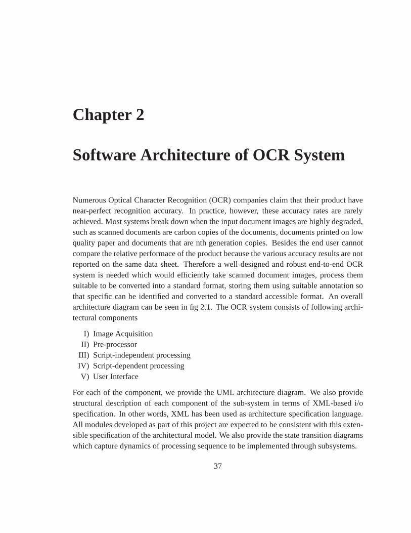
Chapter 2
Software Architecture of OCR System
Numerous Optical Character Recognition (OCR) companies claim that their product havenear-perfect recognition accuracy. In practice, however,these accuracy rates are rarelyachieved. Most systems break down when the input document images are highly degraded,such as scanned documents are carbon copies of the documents, documents printed on lowquality paper and documents that are nth generation copies.Besides the end user cannotcompare the relative performace of the product because the various accuracy results are notreported on the same data sheet. Therefore a well designed and robust end-to-end OCRsystem is needed which would efficiently take scanned document images, process themsuitable to be converted into a standard format, storing them using suitable annotation sothat specific can be identified and converted to a standard accessible format. An overallarchitecture diagram can be seen in fig 2.1. The OCR system consists of following archi-tectural components
I) Image AcquisitionII) Pre-processor
III) Script-independent processingIV) Script-dependent processingV) User Interface
For each of the component, we provide the UML architecture diagram. We also providestructural description of each component of the sub-systemin terms of XML-based i/ospecification. In other words, XML has been used as architecture specification language.All modules developed as part of this project are expected tobe consistent with this exten-sible specification of the architectural model. We also provide the state transition diagramswhich capture dynamics of processing sequence to be implemented through subsystems.
37
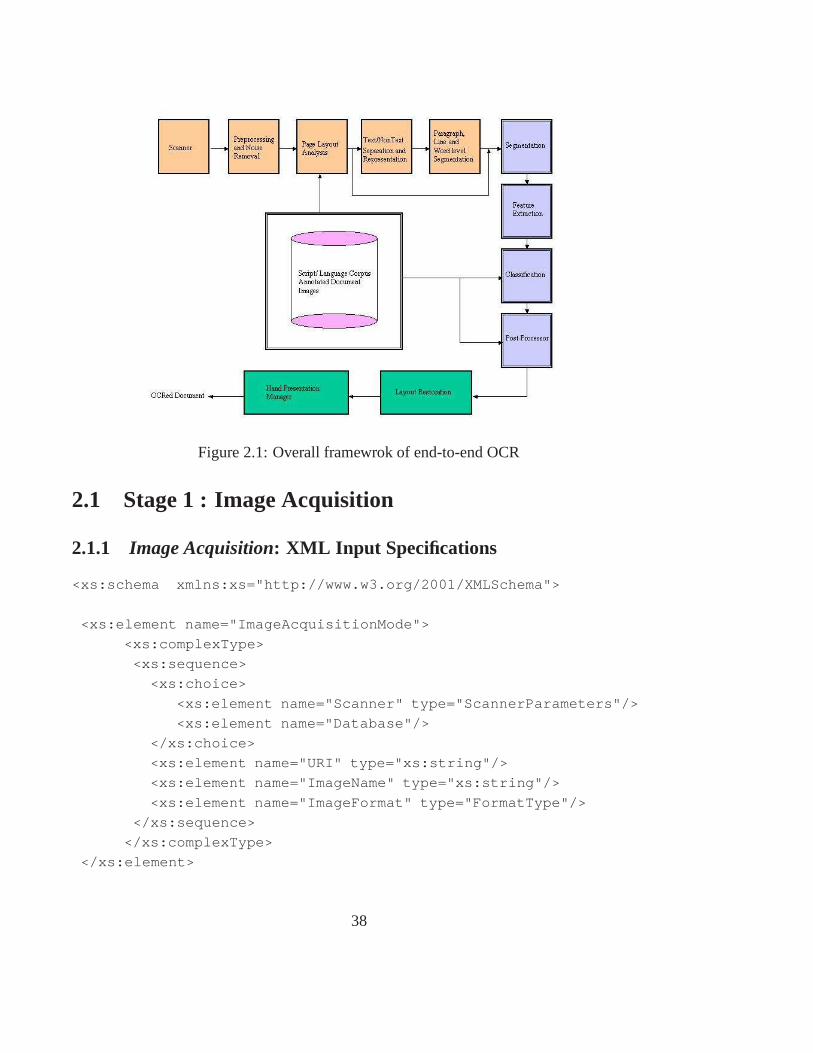
Figure 2.1: Overall framewrok of end-to-end OCR
2.1 Stage 1 : Image Acquisition
2.1.1 Image Acquisition: XML Input Specifications
<xs:schema xmlns:xs="http://www.w3.org/2001/XMLSchema">
<xs:element name="ImageAcquisitionMode">
<xs:complexType>
<xs:sequence>
<xs:choice>
<xs:element name="Scanner" type="ScannerParameters"/>
<xs:element name="Database"/>
</xs:choice>
<xs:element name="URI" type="xs:string"/>
<xs:element name="ImageName" type="xs:string"/>
<xs:element name="ImageFormat" type="FormatType"/>
</xs:sequence>
</xs:complexType>
</xs:element>
38
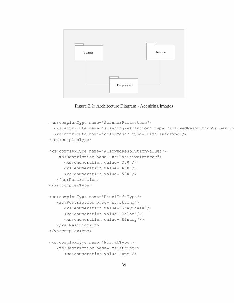
Pre−processor
Scanner Database
Figure 2.2: Architecture Diagram - Acquiring Images
<xs:complexType name="ScannerParameters">
<xs:attribute name="scanningResolution" type="AllowedResolutionValues"/>
<xs:attribute name="colorMode" type="PixelInfoType"/>
</xs:complexType>
<xs:complexType name="AllowedResolutionValues">
<xs:Restriction base="xs:PositiveInteger">
<xs:enumeration value="300"/>
<xs:enumeration value="600"/>
<xs:enumeration value="500"/>
</xs:Restriction>
</xs:complexType>
<xs:complexType name="PixelInfoType">
<xs:Restriction base="xs:string">
<xs:enumeration value="GrayScale"/>
<xs:enumeration value="Color"/>
<xs:enumeration value="Binary"/>
</xs:Restriction>
</xs:complexType>
<xs:complexType name="FormatType">
<xs:Restriction base="xs:string">
<xs:enumeration value="ppm"/>
39

<xs:enumeration value="pgm"/>
<xs:enumeration value="jpg"/>
<xs:enumeration value="bmp"/>
<xs:enumeration value="tif"/>
</xs:Restriction>
</xs:complexType>
</xs:schema>
40
2.1.2 Image Acquisition: XML Output Specifications
<xs:schema xmlns:xs="http://www.w3.org/2001/XMLSchema">
<xs:element name="RawImage">
<xs:complexType>
<xs:sequence>
<xs:element name="ImageName" type="xs:string" />
<xs:element name="ImageURI" type="xs:string" />
</xs:sequence>
<xs:attribute name="ImageEncodingFormat" type="FormatType"/>
<xs:attribute name="ImageWidth" type="xs:positiveInteger"/>
<xs:attribute name="ImageHeight" type="xs:positiveInteger"/>
<xs:attribute name="ImagePixelInfo" type="PixelInfoType"/>
<xs:attribute name="ScanningResolution" type="AllowedResolutionValues"/>
<xs:attribute name="NumberOfBytesPerPixel" type="xs:positiveInteger"/>
</xs:complexType>
</xs:element>
<xs:complexType name="FormatType">
<xs:Restriction base="xs:string">
<xs:enumeration value="ppm"/>
<xs:enumeration value="pgm"/>
<xs:enumeration value="jpg"/>
<xs:enumeration value="bmp"/>
<xs:enumeration value="tif"/>
</xs:Restriction>
</xs:complexType>
<xs:complexType name="PixelInfoType">
<xs:Restriction base="xs:string">
<xs:enumeration value="GrayScale"/>
<xs:enumeration value="Color"/>
<xs:enumeration value="Binary"/>
</xs:Restriction>
</xs:complexType>
<xs:complexType name="AllowedResolutionValues">
<xs:Restriction base="xs:PositiveInteger">
<xs:enumeration value="300"/>
41

(a) (b)
Figure 2.3: GUI snapshots showing the two ways of acquiring the image
<xs:enumeration value="600"/>
<xs:enumeration value="500"/>
</xs:Restriction>
</xs:complexType>
</xs:schema>
42
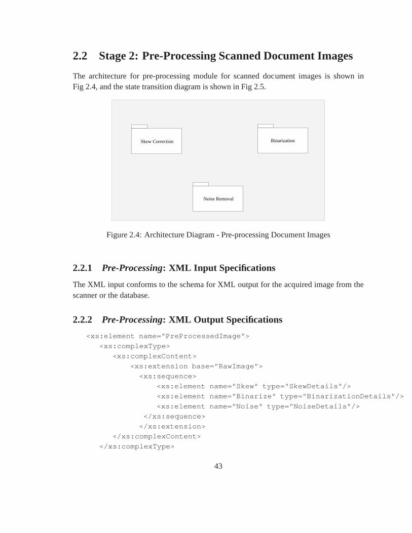
2.2 Stage 2: Pre-Processing Scanned Document Images
The architecture for pre-processing module for scanned document images is shown inFig 2.4, and the state transition diagram is shown in Fig 2.5.
Skew Correction Binarization
Noise Removal
Figure 2.4: Architecture Diagram - Pre-processing Document Images
2.2.1 Pre-Processing: XML Input Specifications
The XML input conforms to the schema for XML output for the acquired image from thescanner or the database.
2.2.2 Pre-Processing: XML Output Specifications
<xs:element name="PreProcessedImage">
<xs:complexType>
<xs:complexContent>
<xs:extension base="RawImage">
<xs:sequence>
<xs:element name="Skew" type="SkewDetails"/>
<xs:element name="Binarize" type="BinarizationDetails"/>
<xs:element name="Noise" type="NoiseDetails"/>
</xs:sequence>
</xs:extension>
</xs:complexContent>
</xs:complexType>
43

</xs:element>
<xs:complexType name="SkewDetails">
<xs:sequence>
<xs:element name="ImageName" type="xs:string" />
<xs:element name="ImageURI" type="xs:string" />
</xs:sequence>
<xs:attribute name="SkewAngleBefore" type="xs:decimal"/>
<xs:attribute name="SkewAngleAfter" type="xs:decimal"/>
<xs:attribute name="AlgorithmName" type="xs:string"/>
</xs:complexType>
<xs:complexType name="BinarizationDetails">
<xs:sequence>
<xs:element name="ImageName" type="xs:string" />
<xs:element name="ImageURI" type="xs:string" />
</xs:sequence>
<xs:attribute name="ThresholdValue" type="xs:integer"/>
<xs:attribute name="AlgorithmName" type="xs:string"/>
</xs:complexType>
<xs:complexType name="NoiseDetails">
<xs:sequence>
<xs:element name="ImageName" type="xs:string" />
<xs:element name="ImageURI" type="xs:string" />
</xs:sequence>
<xs:attribute name="NoiseType" type="xs:string"/>
<xs:attribute name="AlgorithmName" type="xs:string"/>
</xs:complexType>
44
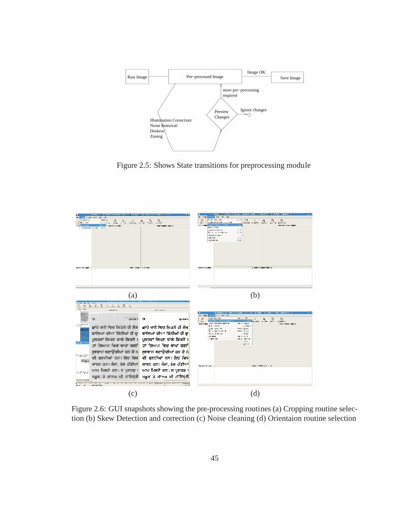
Illumination Correction/Noise Removal/Deskew/Zoning
Raw Image Pre−processed Image Save Image
PreviewChanges
more pre−processingrequired
Image OK
Ignore changes
Figure 2.5: Shows State transitions for preprocessing module
(a) (b)
(c) (d)
Figure 2.6: GUI snapshots showing the pre-processing routines (a) Cropping routine selec-tion (b) Skew Detection and correction (c) Noise cleaning (d) Orientaion routine selection
45
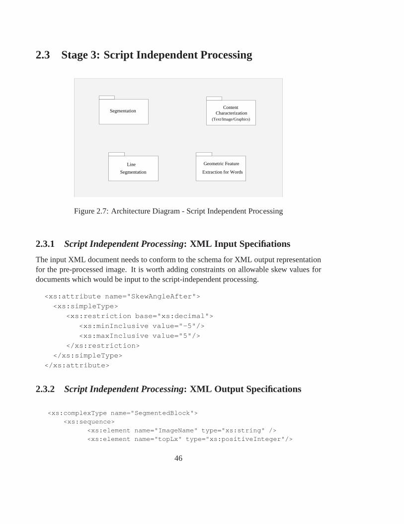
2.3 Stage 3: Script Independent Processing
Segmentation Characterization(Text/Image/Graphics)
Content
Geometric Feature
Extraction for Words
Line
Segmentation
Figure 2.7: Architecture Diagram - Script Independent Processing
2.3.1 Script Independent Processing: XML Input Specifiations
The input XML document needs to conform to the schema for XML output representationfor the pre-processed image. It is worth adding constraintson allowable skew values fordocuments which would be input to the script-independent processing.
<xs:attribute name="SkewAngleAfter">
<xs:simpleType>
<xs:restriction base="xs:decimal">
<xs:minInclusive value="-5"/>
<xs:maxInclusive value="5"/>
</xs:restriction>
</xs:simpleType>
</xs:attribute>
2.3.2 Script Independent Processing: XML Output Specifications
<xs:complexType name="SegmentedBlock"><xs:sequence>
<xs:element name="ImageName" type="xs:string" /><xs:element name="topLx" type="xs:positiveInteger"/>
46
<xs:element name="topLy" type="xs:positiveInteger"/>
<xs:element name="bottomRx" type="xs:positiveInteger"/><xs:element name="bottomRy" type="xs:positiveInteger"/>
</xs:sequence>
</xs:complexType>
<xs:element name="ImageBlock" type="SegmentedBlock"></xs:element>
<xs:element name="GraphicsBlock" type="SegmentedBlock"></xs:element>
<xs:element name="TextBlock">
<xs:complexType><xs:complexContent>
<xs:extension base="SegmentedBlock">
<xs:sequence><xs:element name="TextLine" type="TextLineType" minOccurrs="0"/>
</xs:sequence></xs:extension>
</xs:complexContent>
</xs:complexType></xs:element>
<xs:complexType name="TextLineType">
<xs:complexContent>
<xs:extension base="SegmentedBlock"><xs:sequence>
<xs:element name="TextWord" type="TextWordType" minOccurrs="0"/></xs:sequence>
</xs:extension></xs:complexContent>
</xs:complexType>
47

Pre−processed Image SegmentationModule
Automaticsegmentation
Segment
Manual Segmentation selecting regions
content identification& assign labels
Label ok
Cropping/
No
ToSelectMore
Yes No
ImageSegmented
register/save
register/save
Figure 2.8: Shows state transitions for the script independent module
(a) (b)
Figure 2.9: GUI snapshots showing the script independent module (a) Docstrum (b) ImageSegmentation
2.4 Stage 4: Script Dependent Processing
2.4.1 Script Dependent Processing: XML Input Specifications
The script dependent module processes the text blocks identified by script-independentprocessing. Information about text blocks is incorporatedin the XML element(s)TextBlockwhich incorporate the output information from the script independent module. A text blockcarries information about its bounding box. Further, line segmentation can be attempted bythe script independent module or by the script dependent module− as the strategy may varyfrom script to script. Irrespective of which module does theline/word segmentation, theoutput information about the line bounding box or the word bounding box is stored in theTextLineorTextWordelements organized in theTextBlock→TextLine→TextWordhierarchy.
48
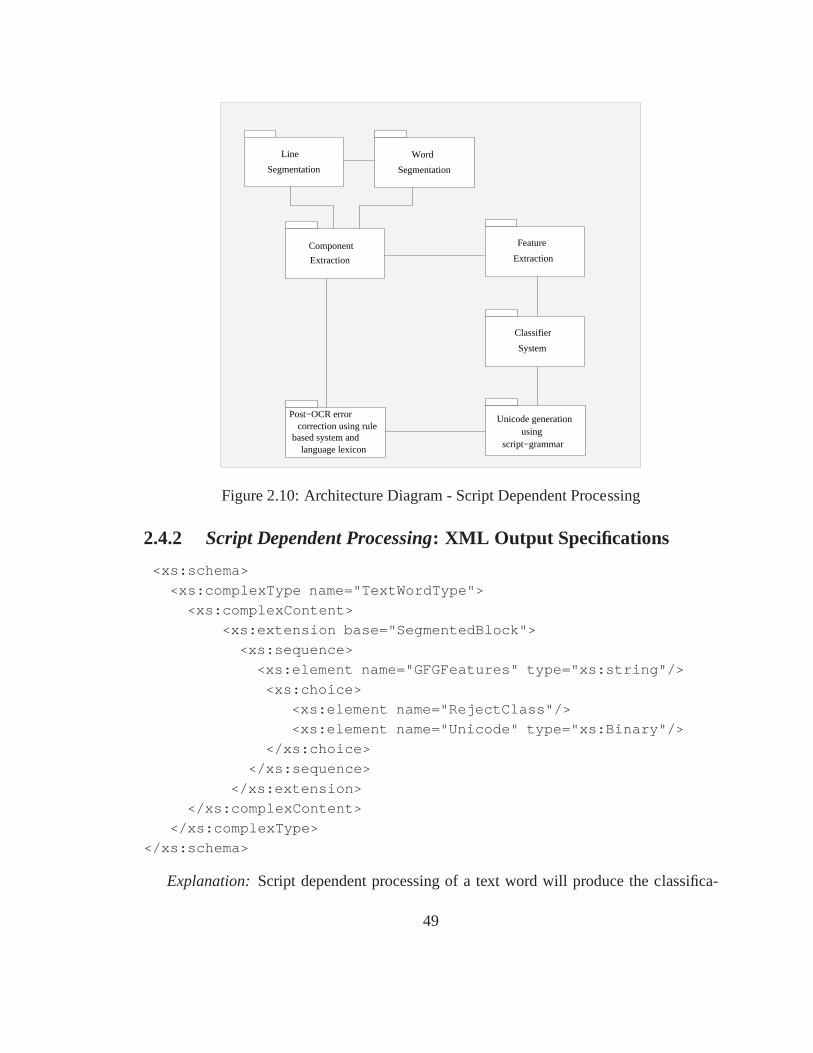
Line
Segmentation
Word
Segmentation
Extraction
Component
Classifier
System
Feature
Extraction
Unicode generation
script−grammarusing
Post−OCR error
language lexiconbased system and
correction using rule
Figure 2.10: Architecture Diagram - Script Dependent Processing
2.4.2 Script Dependent Processing: XML Output Specifications
<xs:schema>
<xs:complexType name="TextWordType">
<xs:complexContent>
<xs:extension base="SegmentedBlock">
<xs:sequence>
<xs:element name="GFGFeatures" type="xs:string"/>
<xs:choice>
<xs:element name="RejectClass"/>
<xs:element name="Unicode" type="xs:Binary"/>
</xs:choice>
</xs:sequence>
</xs:extension>
</xs:complexContent>
</xs:complexType>
</xs:schema>
Explanation: Script dependent processing of a text word will produce the classifica-
49
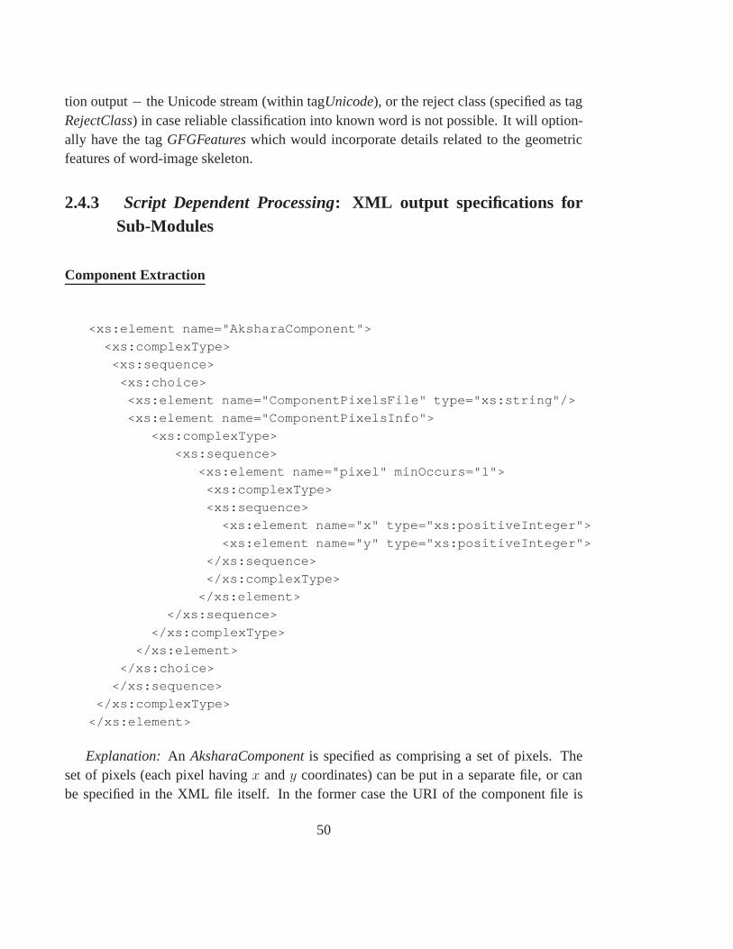
tion output− the Unicode stream (within tagUnicode), or the reject class (specified as tagRejectClass) in case reliable classification into known word is not possible. It will option-ally have the tagGFGFeatureswhich would incorporate details related to the geometricfeatures of word-image skeleton.
2.4.3 Script Dependent Processing: XML output specifications forSub-Modules
Component Extraction
<xs:element name="AksharaComponent">
<xs:complexType>
<xs:sequence>
<xs:choice>
<xs:element name="ComponentPixelsFile" type="xs:string"/>
<xs:element name="ComponentPixelsInfo">
<xs:complexType>
<xs:sequence>
<xs:element name="pixel" minOccurs="1">
<xs:complexType>
<xs:sequence>
<xs:element name="x" type="xs:positiveInteger">
<xs:element name="y" type="xs:positiveInteger">
</xs:sequence>
</xs:complexType>
</xs:element>
</xs:sequence>
</xs:complexType>
</xs:element>
</xs:choice>
</xs:sequence>
</xs:complexType>
</xs:element>
Explanation: An AksharaComponentis specified as comprising a set of pixels. Theset of pixels (each pixel havingx andy coordinates) can be put in a separate file, or canbe specified in the XML file itself. In the former case the URI ofthe component file is
50
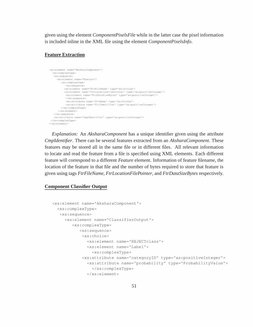
given using the elementComponentPixelsFilewhile in the latter case the pixel informationis included inline in the XML file using the elementComponentPixelsInfo.
Feature Extraction
<xs:element name="AksharaComponent"><xs:complexType><xs:sequence>
<xs:element name="Feature"><xs:complexType>
<xs:sequence><xs:element name="FtrFileName" type="xs:string"><xs:element name="FtrLocationFilePointer" type="xs:positiveInteger"><xs:element name="FtrDataSizeBytes" type="xs:positiveInteger"></xs:sequence><xs:attribute name="FtrName" type="xs:string"><xs:attribute name="FtrIdentifier" type="xs:positiveInteger">
</xs:complexType></xs:element>
</xs:sequence><xs:attribute name="CmpIdentifier" type="xs:positiveInteger">
</xs:complexType></xs:element>
Explanation: An AksharaComponenthas a unique identifier given using the attributeCmpIdentifier. There can be several features extracted from anAksharaComponent. Thesefeatures may be stored all in the same file or in different files. All relevant informationto locate and read the feature from a file is specified using XMLelements. Each differentfeature will correspond to a differentFeatureelement. Information of feature filename, thelocation of the feature in that file and the number of bytes required to store that feature isgiven using tagsFtrFileName, FtrLocationFilePointer, andFtrDataSizeBytesrespectively.
Component Classifier Output
<xs:element name="AksharaComponent"><xs:complexType>
<xs:sequence>
<xs:element name="ClassifierOutput"><xs:complexType>
<xs:sequence><xs:choice>
<xs:element name="REJECTclass">
<xs:element name="Label"><xs:complexType>
<xs:attribute name="categoryID" type="xs:positiveInteger"><xs:attribute name="probability" type="ProbabilityValue">
</xs:complexType></xs:element>
51
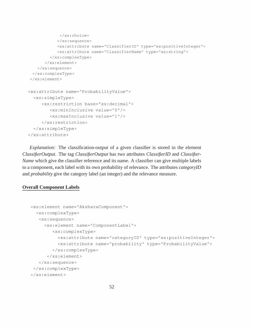
</xs:choice>
</xs:sequence><xs:attribute name="ClassifierID" type="xs:positiveInteger">
<xs:attribute name="ClassifierName" type="xs:string">
</xs:complexType></xs:element>
</xs:sequence></xs:complexType>
</xs:element>
<xs:attribute name="ProbabilityValue">
<xs:simpleType>
<xs:restriction base="xs:decimal">
<xs:minInclusive value="0"/>
<xs:maxInclusive value="1"/>
</xs:restriction>
</xs:simpleType>
</xs:attribute>
Explanation: The classification-output of a given classifier is stored in the elementClassifierOutput. The tagClassifierOutputhas two attributesClassifierIDandClassifier-Namewhich give the classifier reference and its name. A classifiercan give multiple labelsto a component, each label with its own probability of relevance. The attributescategoryIDandprobabilitygive the category label (an integer) and the relevance measure.
Overall Component Labels
<xs:element name="AksharaComponent">
<xs:complexType>
<xs:sequence>
<xs:element name="ComponentLabel">
<xs:complexType>
<xs:attribute name="categoryID" type="xs:positiveInteger">
<xs:attribute name="probability" type="ProbabilityValue">
</xs:complexType>
</xs:element>
</xs:sequence>
</xs:complexType>
</xs:element>
52
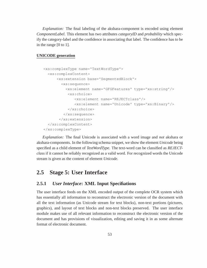
Explanation: The final labeling of the akshara-component is encoded usingelementComponentLabel. This element has two attributescategoryIDandprobabilitywhich spec-ify the category-label and the confidence in associating that label. The confidence has to bein the range [0 to 1].
UNICODE generation
<xs:complexType name="TextWordType">
<xs:complexContent>
<xs:extension base="SegmentedBlock">
<xs:sequence>
<xs:element name="GFGFeatures" type="xs:string"/>
<xs:choice>
<xs:element name="REJECTclass"/>
<xs:element name="Unicode" type="xs:Binary"/>
</xs:choice>
</xs:sequence>
</xs:extension>
</xs:complexContent>
</xs:complexType>
Explanation: The final Unicode is associated with a word image andnot akshara orakshara-components. In the following schema snippet, we show the elementUnicodebeingspecified as a child element ofTextWordType. The text-word can be classified asREJECT-classif it cannot be reliably recognized as a valid word. For recognized words the Unicodestream is given as the content of elementUnicode.
2.5 Stage 5: User Interface
2.5.1 User Interface: XML Input Specifiations
The user interface feeds on the XML encoded output of the complete OCR system whichhas essentially all information to reconstruct the electronic version of the document withall the text information (as Unicode stream for text blocks), non-text portions (pictures,graphics), and layout of text blocks and non-text blocks preserved. The user interfacemodule makes use of all relevant information to reconstructthe electronic version of thedocument and has provisions of visualization, editing and saving it in as some alternateformat of electronic document.
53
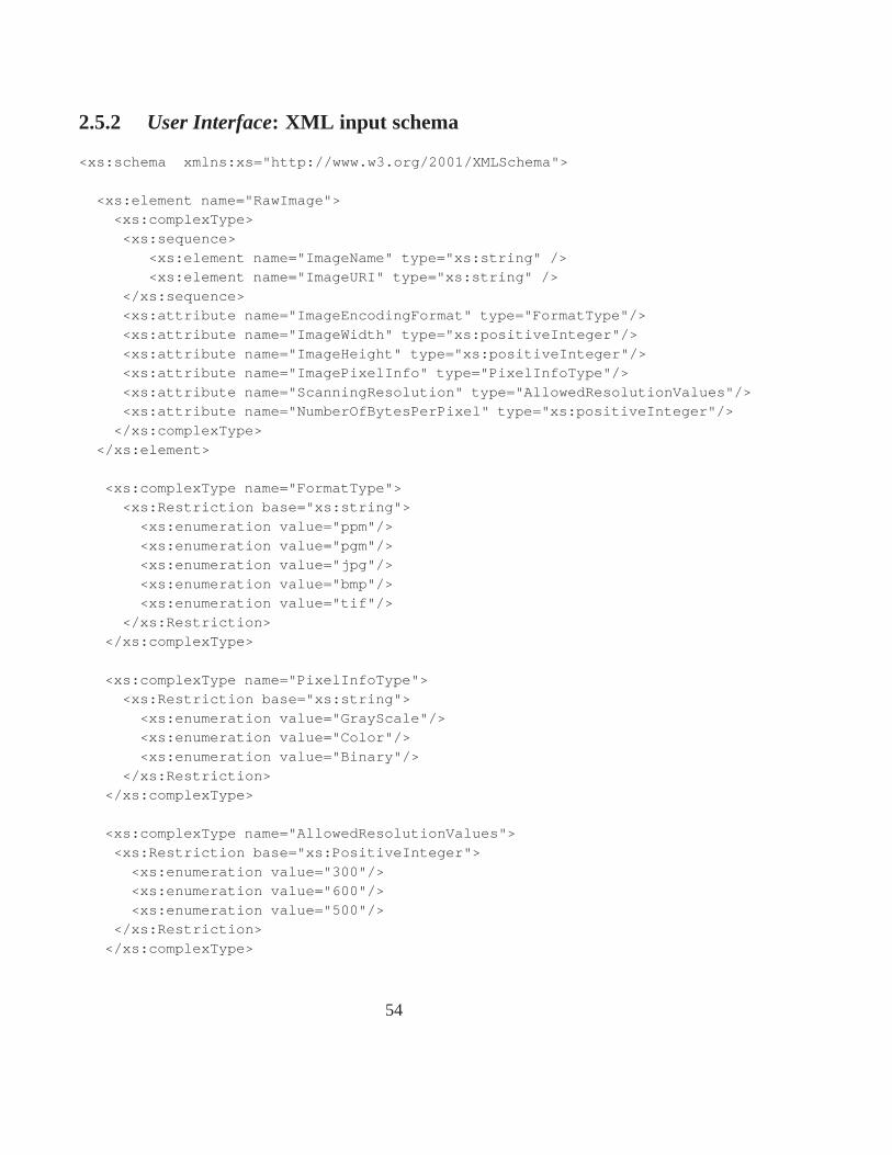
2.5.2 User Interface: XML input schema
<xs:schema xmlns:xs="http://www.w3.org/2001/XMLSchema">
<xs:element name="RawImage"><xs:complexType>
<xs:sequence>
<xs:element name="ImageName" type="xs:string" /><xs:element name="ImageURI" type="xs:string" />
</xs:sequence><xs:attribute name="ImageEncodingFormat" type="FormatType"/>
<xs:attribute name="ImageWidth" type="xs:positiveInteger"/>
<xs:attribute name="ImageHeight" type="xs:positiveInteger"/><xs:attribute name="ImagePixelInfo" type="PixelInfoType"/>
<xs:attribute name="ScanningResolution" type="AllowedResolutionValues"/><xs:attribute name="NumberOfBytesPerPixel" type="xs:positiveInteger"/>
</xs:complexType>
</xs:element>
<xs:complexType name="FormatType"><xs:Restriction base="xs:string">
<xs:enumeration value="ppm"/>
<xs:enumeration value="pgm"/><xs:enumeration value="jpg"/>
<xs:enumeration value="bmp"/><xs:enumeration value="tif"/>
</xs:Restriction></xs:complexType>
<xs:complexType name="PixelInfoType"><xs:Restriction base="xs:string">
<xs:enumeration value="GrayScale"/><xs:enumeration value="Color"/>
<xs:enumeration value="Binary"/>
</xs:Restriction></xs:complexType>
<xs:complexType name="AllowedResolutionValues">
<xs:Restriction base="xs:PositiveInteger">
<xs:enumeration value="300"/><xs:enumeration value="600"/>
<xs:enumeration value="500"/></xs:Restriction>
</xs:complexType>
54
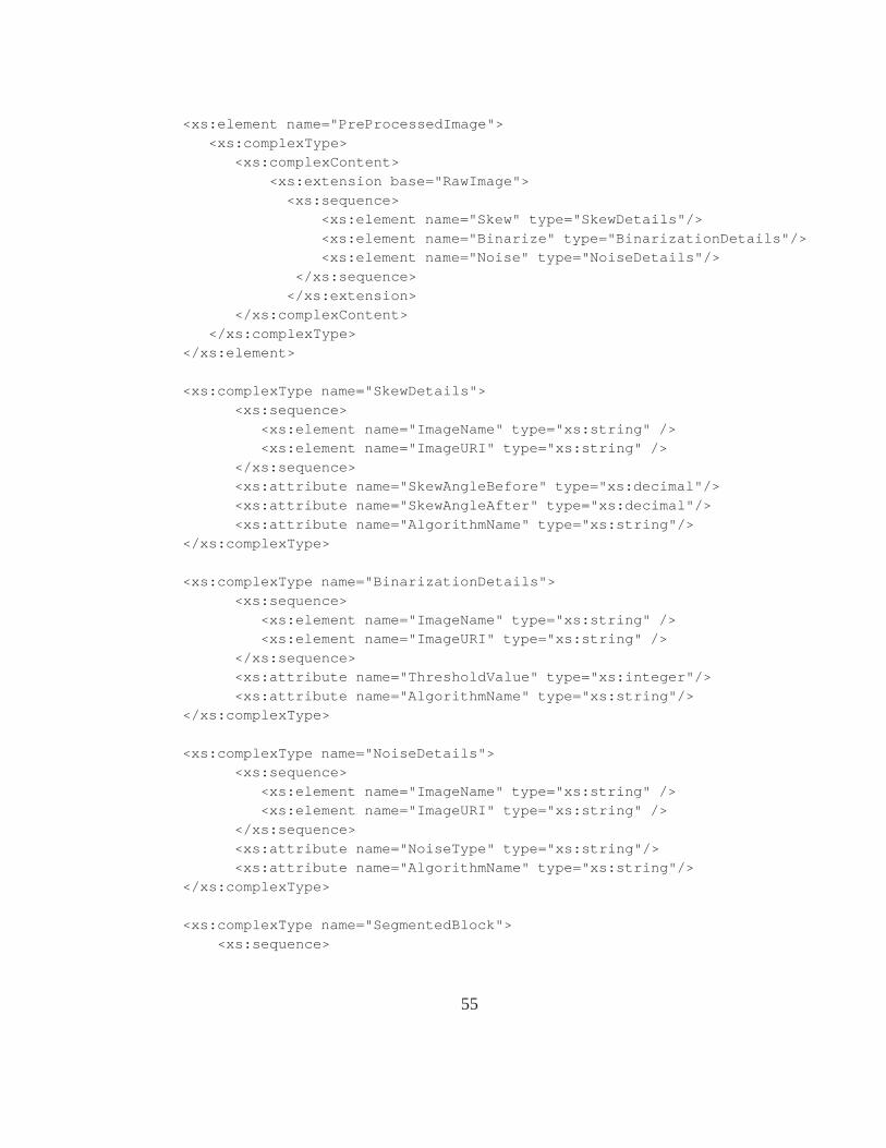
<xs:element name="PreProcessedImage">
<xs:complexType><xs:complexContent>
<xs:extension base="RawImage">
<xs:sequence><xs:element name="Skew" type="SkewDetails"/>
<xs:element name="Binarize" type="BinarizationDetails"/><xs:element name="Noise" type="NoiseDetails"/>
</xs:sequence>
</xs:extension></xs:complexContent>
</xs:complexType></xs:element>
<xs:complexType name="SkewDetails">
<xs:sequence>
<xs:element name="ImageName" type="xs:string" /><xs:element name="ImageURI" type="xs:string" />
</xs:sequence><xs:attribute name="SkewAngleBefore" type="xs:decimal"/>
<xs:attribute name="SkewAngleAfter" type="xs:decimal"/>
<xs:attribute name="AlgorithmName" type="xs:string"/></xs:complexType>
<xs:complexType name="BinarizationDetails">
<xs:sequence>
<xs:element name="ImageName" type="xs:string" /><xs:element name="ImageURI" type="xs:string" />
</xs:sequence><xs:attribute name="ThresholdValue" type="xs:integer"/>
<xs:attribute name="AlgorithmName" type="xs:string"/></xs:complexType>
<xs:complexType name="NoiseDetails"><xs:sequence>
<xs:element name="ImageName" type="xs:string" /><xs:element name="ImageURI" type="xs:string" />
</xs:sequence>
<xs:attribute name="NoiseType" type="xs:string"/><xs:attribute name="AlgorithmName" type="xs:string"/>
</xs:complexType>
<xs:complexType name="SegmentedBlock">
<xs:sequence>
55
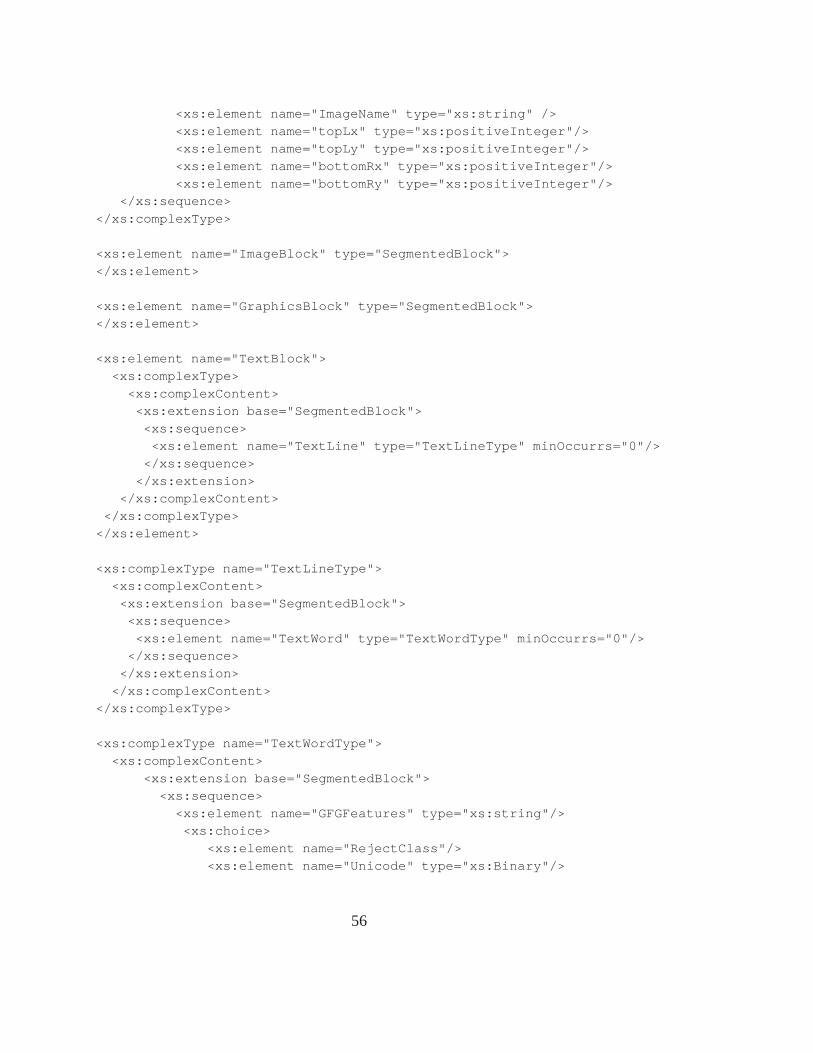
<xs:element name="ImageName" type="xs:string" />
<xs:element name="topLx" type="xs:positiveInteger"/><xs:element name="topLy" type="xs:positiveInteger"/>
<xs:element name="bottomRx" type="xs:positiveInteger"/>
<xs:element name="bottomRy" type="xs:positiveInteger"/></xs:sequence>
</xs:complexType>
<xs:element name="ImageBlock" type="SegmentedBlock">
</xs:element>
<xs:element name="GraphicsBlock" type="SegmentedBlock"></xs:element>
<xs:element name="TextBlock">
<xs:complexType>
<xs:complexContent><xs:extension base="SegmentedBlock">
<xs:sequence><xs:element name="TextLine" type="TextLineType" minOccurrs="0"/>
</xs:sequence>
</xs:extension></xs:complexContent>
</xs:complexType></xs:element>
<xs:complexType name="TextLineType"><xs:complexContent>
<xs:extension base="SegmentedBlock"><xs:sequence>
<xs:element name="TextWord" type="TextWordType" minOccurrs="0"/></xs:sequence>
</xs:extension>
</xs:complexContent></xs:complexType>
<xs:complexType name="TextWordType">
<xs:complexContent>
<xs:extension base="SegmentedBlock"><xs:sequence>
<xs:element name="GFGFeatures" type="xs:string"/><xs:choice>
<xs:element name="RejectClass"/>
<xs:element name="Unicode" type="xs:Binary"/>
56
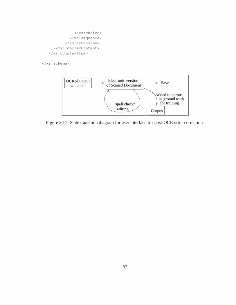
</xs:choice>
</xs:sequence></xs:extension>
</xs:complexContent>
</xs:complexType>
</xs:schema>
OCRed OuputUnicode
Electronic versionof Scaned Document
Save
Corpus
spell check/editing
Added to corpus as ground truthfor training
Figure 2.11: State transition diagram for user interface for post-OCR error correction
57

Chapter 3
Pre-processing of Scanned Documents
3.1 Introduction
In many applications involving character recognition fromdigitized document images, theinput images are first binarized to form two level images. However, direct binarizationof such images often results in unsatisfactory performancebecause of the poor quality ofthe input images. Consequently, it is usual to preprocess such images in order to enhancethe edges in the presence of noise and other types of distortions that occur during thescanning process. Edge enhancement and noise reduction areconflicting requirements forlinear, space invariant filters. Therefore, it is necessaryto employ nonlinear and/or adaptivetechniques for processing document images prior to binarization.
The role of preprocessing module is to take the input document image(either a gray-scale image or a color image) and make it fit for subsequent processing to achieve bestresults.There are a variety of algorithms that together constitute the pre-processing module.The details for each of the pre-processing feature is explained below.
i. Text direction detection and correctionii. Skew detection and correction
iii. Noise removaliv. Binarizationv. Cropping/Zoning
The differnent pre-processing function were contributed by the following consortiummembers.
i. Text direction detection and correction -ISI Kolkatta .
ii. Skew detection and correction -IIIT Hyderabad
59
iii. Noise removal -ISI Kolkatta
iv. Binarization -IIT Delhi and ISI Kolkatta
v. Cropping/Zoning -IIT Delhi
3.2 Text Direction : Detection and correction of portrait/landscapemode
A document may be inadvertently scanned in a landscape mode when the text is aligned inportrait mode or vice versa. There should be automatic way ofcorrecting the orientation ofsuch scanned document. The problem is intensified when thereis skew in addition to themode mistake. The current algorithm detects the mode mistake, if any and corrects it if thedocument is printed in Bangla or Devanagari.
3.2.1 Requirement analysis
It is assumed that the image is scanned at 300 dpi and it contains predominantly text mat-ter (say 80% of the area). It works on two tone image. Single ormulti-column image isequally acceptable. Attempts have been made to make time complexity low and detectionand correction accuracy high. So, the central portion of theimage is taken for processing.While detection part will support all types of printed text (English, Bangla, Hindi, Gur-mukhi, Tamil) the correction part has been script specific and we work here on Bangla andDevanagari only.
At present we have taken .PGM image in 1 byte/pixel format forboth input and output.It will work on Windows 98/Windows XP/Windows 2000 and with minor modification onLinux platform.
Since it works on two-tone image, at first a binarization and noise cleaning algorithmshould run on the original image data.
3.2.2 Software development
To reduce time, the software runs on a 10 square inch in the central part of the documentimage, which is 1000x1000 pixels at 300 dpi scanning. If a mode mismatch occurs, it mayoccur in two rotations i.e. +90 degrees or -90 degrees. So, the algorithm works at twostages: (a) detection of wrong mode, (b) detection of +90 or 90 degree. Finally, the imageis given counter-rotation in that angle to have the correct orientation.
60
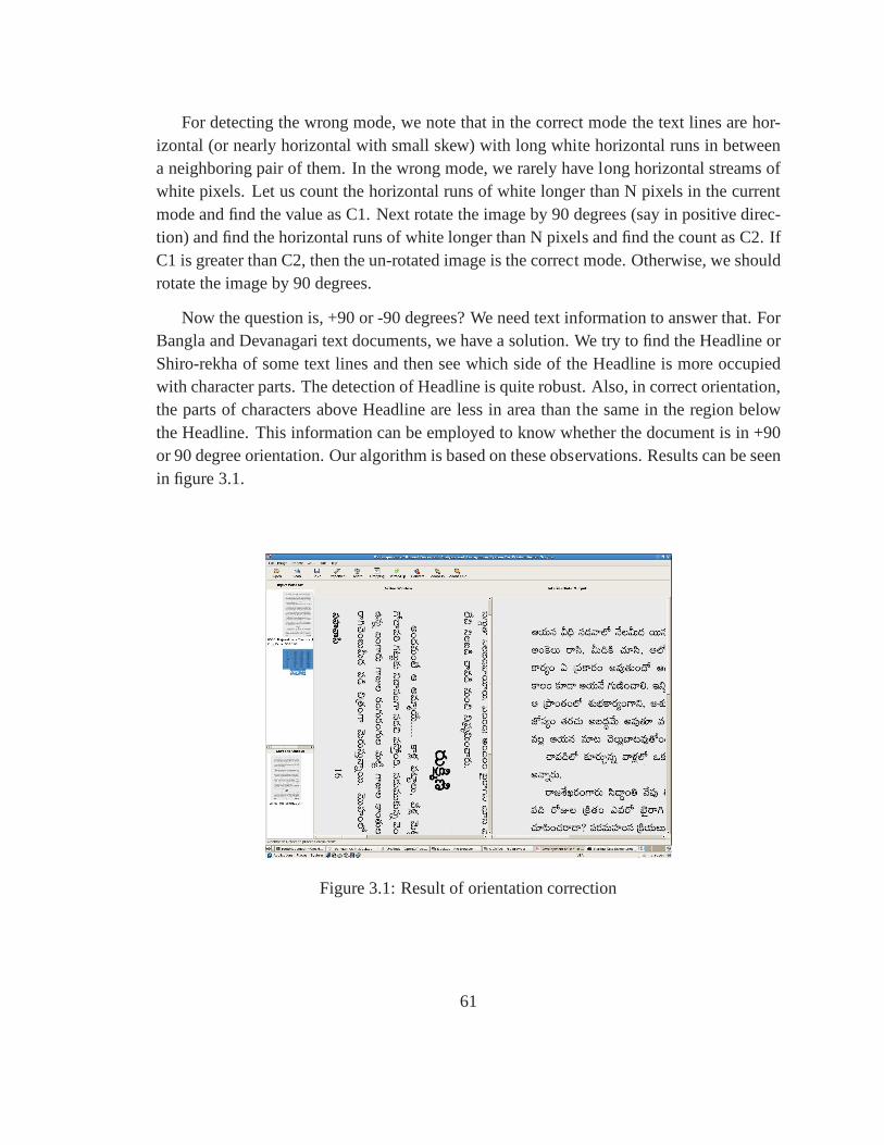
For detecting the wrong mode, we note that in the correct modethe text lines are hor-izontal (or nearly horizontal with small skew) with long white horizontal runs in betweena neighboring pair of them. In the wrong mode, we rarely have long horizontal streams ofwhite pixels. Let us count the horizontal runs of white longer than N pixels in the currentmode and find the value as C1. Next rotate the image by 90 degrees (say in positive direc-tion) and find the horizontal runs of white longer than N pixels and find the count as C2. IfC1 is greater than C2, then the un-rotated image is the correct mode. Otherwise, we shouldrotate the image by 90 degrees.
Now the question is, +90 or -90 degrees? We need text information to answer that. ForBangla and Devanagari text documents, we have a solution. Wetry to find the Headline orShiro-rekha of some text lines and then see which side of the Headline is more occupiedwith character parts. The detection of Headline is quite robust. Also, in correct orientation,the parts of characters above Headline are less in area than the same in the region belowthe Headline. This information can be employed to know whether the document is in +90or 90 degree orientation. Our algorithm is based on these observations. Results can be seenin figure 3.1.
Figure 3.1: Result of orientation correction
61
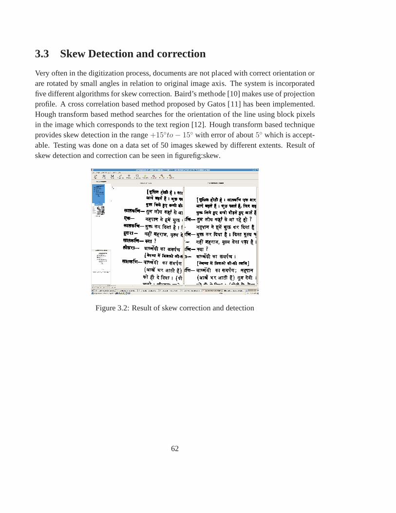
3.3 Skew Detection and correction
Very often in the digitization process, documents are not placed with correct orientation orare rotated by small angles in relation to original image axis. The system is incorporatedfive different algorithms for skew correction. Baird’s methode [10] makes use of projectionprofile. A cross correlation based method proposed by Gatos [11] has been implemented.Hough transform based method searches for the orientation of the line using block pixelsin the image which corresponds to the text region [12]. Houghtransform based techniqueprovides skew detection in the range+15◦to− 15◦ with error of about5◦ which is accept-able. Testing was done on a data set of 50 images skewed by different extents. Result ofskew detection and correction can be seen in figurefig:skew.
Figure 3.2: Result of skew correction and detection
62
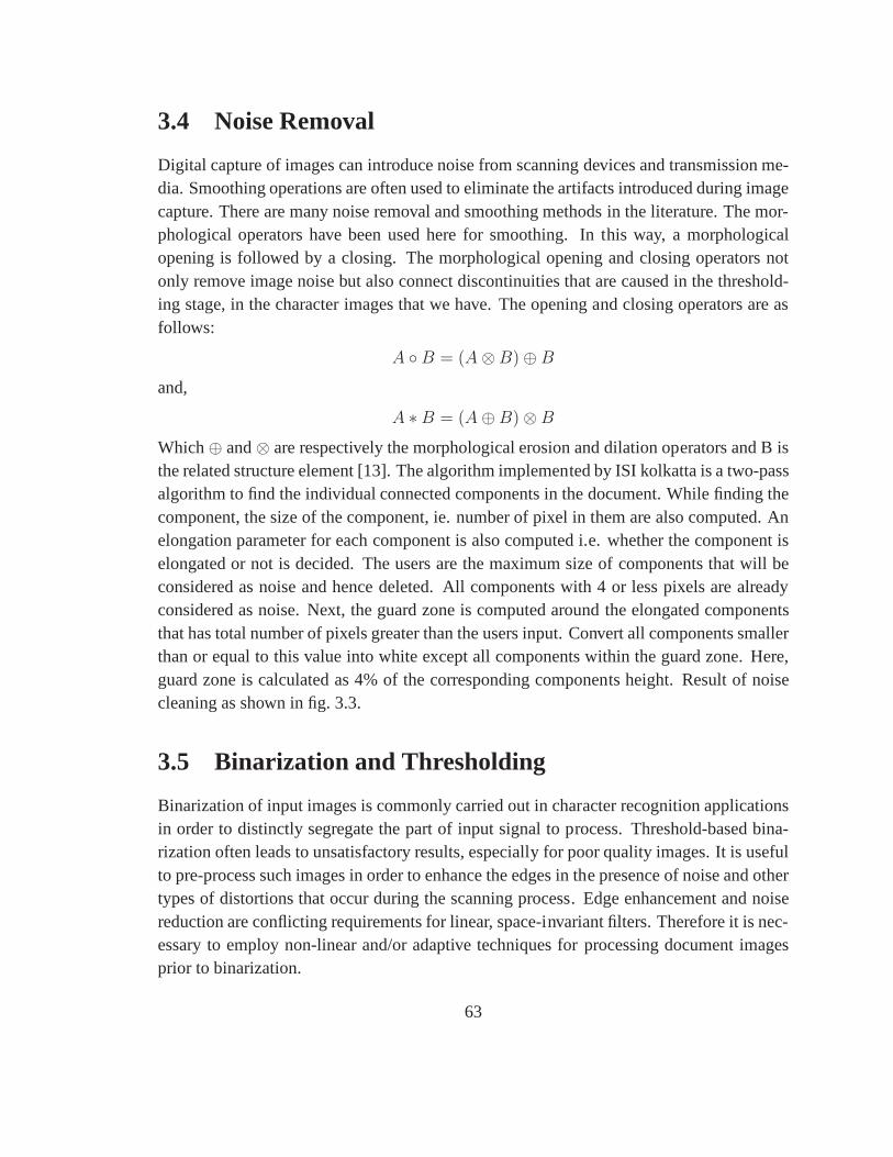
3.4 Noise Removal
Digital capture of images can introduce noise from scanningdevices and transmission me-dia. Smoothing operations are often used to eliminate the artifacts introduced during imagecapture. There are many noise removal and smoothing methodsin the literature. The mor-phological operators have been used here for smoothing. In this way, a morphologicalopening is followed by a closing. The morphological openingand closing operators notonly remove image noise but also connect discontinuities that are caused in the threshold-ing stage, in the character images that we have. The opening and closing operators are asfollows:
A ◦B = (A⊗B)⊕ B
and,
A ∗B = (A⊕B)⊗ B
Which⊕ and⊗ are respectively the morphological erosion and dilation operators and B isthe related structure element [13]. The algorithm implemented by ISI kolkatta is a two-passalgorithm to find the individual connected components in thedocument. While finding thecomponent, the size of the component, ie. number of pixel in them are also computed. Anelongation parameter for each component is also computed i.e. whether the component iselongated or not is decided. The users are the maximum size ofcomponents that will beconsidered as noise and hence deleted. All components with 4or less pixels are alreadyconsidered as noise. Next, the guard zone is computed aroundthe elongated componentsthat has total number of pixels greater than the users input.Convert all components smallerthan or equal to this value into white except all components within the guard zone. Here,guard zone is calculated as 4% of the corresponding components height. Result of noisecleaning as shown in fig. 3.3.
3.5 Binarization and Thresholding
Binarization of input images is commonly carried out in character recognition applicationsin order to distinctly segregate the part of input signal to process. Threshold-based bina-rization often leads to unsatisfactory results, especially for poor quality images. It is usefulto pre-process such images in order to enhance the edges in the presence of noise and othertypes of distortions that occur during the scanning process. Edge enhancement and noisereduction are conflicting requirements for linear, space-invariant filters. Therefore it is nec-essary to employ non-linear and/or adaptive techniques forprocessing document imagesprior to binarization.
63
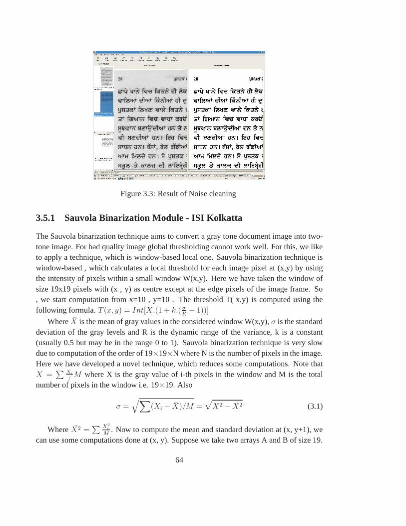
Figure 3.3: Result of Noise cleaning
3.5.1 Sauvola Binarization Module - ISI Kolkatta
The Sauvola binarization technique aims to convert a gray tone document image into two-tone image. For bad quality image global thresholding cannot work well. For this, we liketo apply a technique, which is window-based local one. Sauvola binarization technique iswindow-based , which calculates a local threshold for each image pixel at (x,y) by usingthe intensity of pixels within a small window W(x,y). Here wehave taken the window ofsize 19x19 pixels with (x , y) as centre except at the edge pixels of the image frame. So, we start computation from x=10 , y=10 . The threshold T( x,y)is computed using thefollowing formula.T (x, y) = Int[X.(1 + k.( σ
R− 1))]
WhereX is the mean of gray values in the considered window W(x,y),σ is the standarddeviation of the gray levels and R is the dynamic range of the variance, k is a constant(usually 0.5 but may be in the range 0 to 1). Sauvola binarization technique is very slowdue to computation of the order of 19×19×N where N is the number of pixels in the image.Here we have developed a novel technique, which reduces somecomputations. Note thatX =
∑
Xi
/M where X is the gray value of i-th pixels in the window and M is the total
number of pixels in the window i.e. 19×19. Also
σ =√
∑
(Xi − X)/M =√
X2 − X2 (3.1)
WhereX2 =∑ X2
i
M. Now to compute the mean and standard deviation at (x, y+1), we
can use some computations done at (x, y). Suppose we take two arrays A and B of size 19.
64
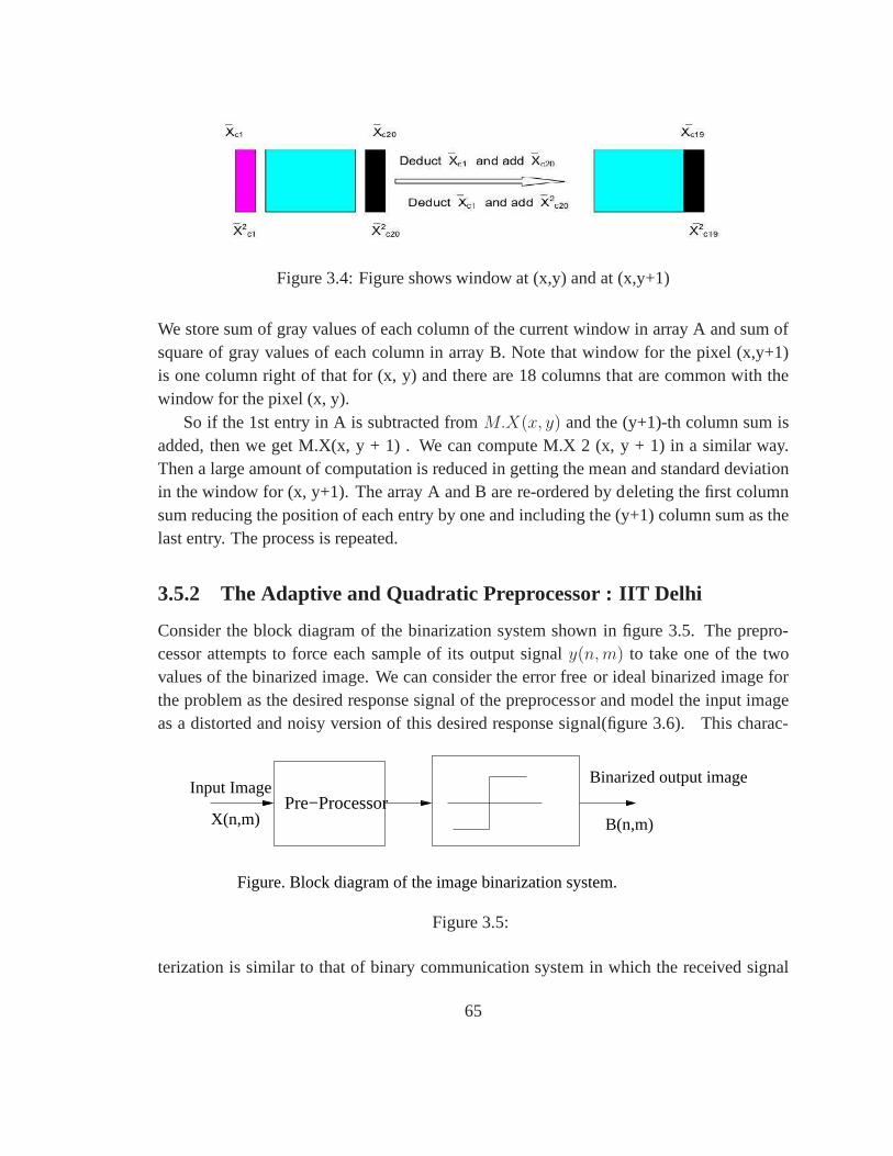
Figure 3.4: Figure shows window at (x,y) and at (x,y+1)
We store sum of gray values of each column of the current window in array A and sum ofsquare of gray values of each column in array B. Note that window for the pixel (x,y+1)is one column right of that for (x, y) and there are 18 columns that are common with thewindow for the pixel (x, y).
So if the 1st entry in A is subtracted fromM.X(x, y) and the (y+1)-th column sum isadded, then we get M.X(x, y + 1) . We can compute M.X 2 (x, y + 1) ina similar way.Then a large amount of computation is reduced in getting the mean and standard deviationin the window for (x, y+1). The array A and B are re-ordered by deleting the first columnsum reducing the position of each entry by one and including the (y+1) column sum as thelast entry. The process is repeated.
3.5.2 The Adaptive and Quadratic Preprocessor : IIT Delhi
Consider the block diagram of the binarization system shownin figure 3.5. The prepro-cessor attempts to force each sample of its output signaly(n, m) to take one of the twovalues of the binarized image. We can consider the error freeor ideal binarized image forthe problem as the desired response signal of the preprocessor and model the input imageas a distorted and noisy version of this desired response signal(figure 3.6). This charac-
X(n,m)
Binarized output image
B(n,m)
Figure. Block diagram of the image binarization system.
Pre−ProcessorInput Image
Figure 3.5:
terization is similar to that of binary communication system in which the received signal
65
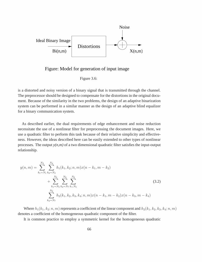
DistortionsIdeal Binary Image
Bi(n,m) X(n,m)
Noise
Figure: Model for generation of input image
Figure 3.6:
is a distorted and noisy version of a binary signal that is transmitted through the channel.The preprocessor should be designed to compensate for the distortions in the original docu-ment. Because of the similarity in the two problems, the design of an adaptive binarizationsystem can be performed in a similar manner as the design of anadaptive blind equalizerfor a binary communication system.
As described earlier, the dual requirements of edge enhancement and noise reductionnecessitate the use of a nonlinear filter for preprocessing the document images. Here, weuse a quadratic filter to perform this task because of their relative simplicity and effective-ness. However, the ideas described here can be easily extended to other types of nonlinearprocesses. The outputy(n,m)of a two dimensional quadratic filter satisfies the input-outputrelationship.
y(n, m) =
N2∑
k1=N1
N4∑
k2=N3
h1(k1, k2; n, m)x(n− k1, m− k2)
+
N6∑
k1=N5
N8∑
k2=N7
N6∑
k=N5
N8∑
k4=N7
h2(k1, k2, k3, k4; n, m)x(n− k1, m− k2)x(n− k3, m− k4)
(3.2)
Whereh1(k1, k2; n, m) represents a coefficient of the linear component andh2(k1, k2, k3, k4; n, m)
denotes a coefficient of the homogeneous quadratic component of the filter.It is common practice to employ a symmetric kernel for the homogeneous quadratic
66
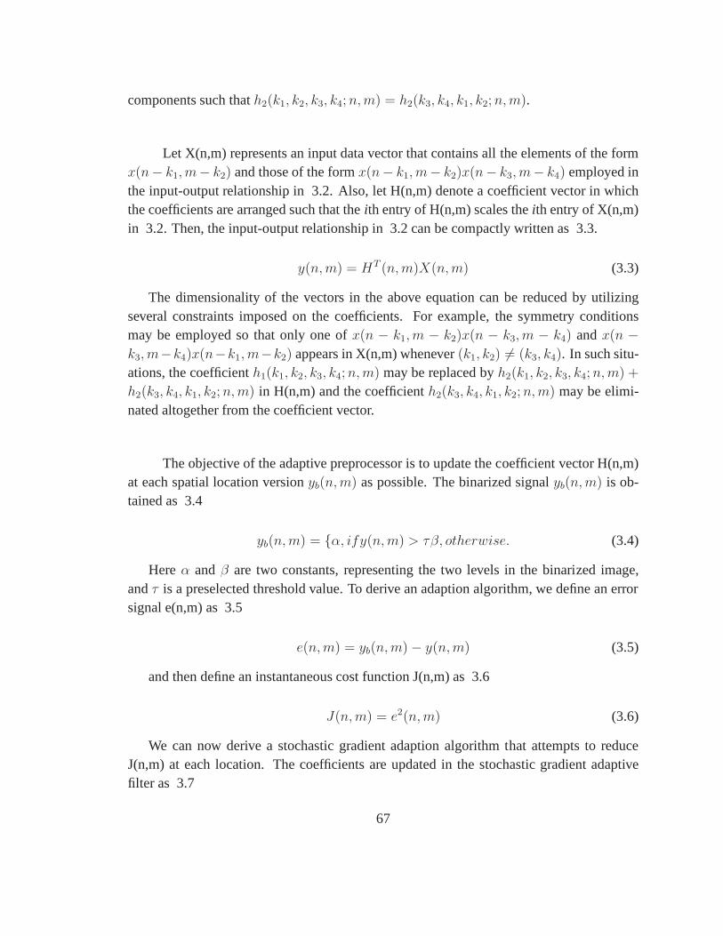
components such thath2(k1, k2, k3, k4; n, m) = h2(k3, k4, k1, k2; n, m).
Let X(n,m) represents an input data vector that contains allthe elements of the formx(n− k1, m− k2) and those of the formx(n− k1, m− k2)x(n− k3, m− k4) employed inthe input-output relationship in 3.2. Also, let H(n,m) denote a coefficient vector in whichthe coefficients are arranged such that theith entry of H(n,m) scales theith entry of X(n,m)in 3.2. Then, the input-output relationship in 3.2 can be compactly written as 3.3.
y(n, m) = HT (n, m)X(n, m) (3.3)
The dimensionality of the vectors in the above equation can be reduced by utilizingseveral constraints imposed on the coefficients. For example, the symmetry conditionsmay be employed so that only one ofx(n − k1, m − k2)x(n − k3, m − k4) andx(n −k3, m−k4)x(n−k1, m−k2) appears in X(n,m) whenever(k1, k2) 6= (k3, k4). In such situ-ations, the coefficienth1(k1, k2, k3, k4; n, m) may be replaced byh2(k1, k2, k3, k4; n, m) +
h2(k3, k4, k1, k2; n, m) in H(n,m) and the coefficienth2(k3, k4, k1, k2; n, m) may be elimi-nated altogether from the coefficient vector.
The objective of the adaptive preprocessor is to update the coefficient vector H(n,m)at each spatial location versionyb(n, m) as possible. The binarized signalyb(n, m) is ob-tained as 3.4
yb(n, m) = {α, ify(n, m) > τβ, otherwise. (3.4)
Hereα andβ are two constants, representing the two levels in the binarized image,andτ is a preselected threshold value. To derive an adaption algorithm, we define an errorsignal e(n,m) as 3.5
e(n, m) = yb(n, m)− y(n, m) (3.5)
and then define an instantaneous cost function J(n,m) as 3.6
J(n, m) = e2(n, m) (3.6)
We can now derive a stochastic gradient adaption algorithm that attempts to reduceJ(n,m) at each location. The coefficients are updated in the stochastic gradient adaptivefilter as 3.7
67
H(n, m + 1) = H(n, m)− µ
2
δ
δH(n, m)J(n, m) = H(n, m) + µe(n, m)X(n, m)
Whereµ is a small, positive step size parameter that controls the convergence, trackingand steady state characteristics of the adaptive filter. In the above derivation, we assumedthat the adaption is performed along the rows of an image. Thecomplete algorithm foradaptive preprocessing and binarization is given in Table 3.1.
Table 3.1: ADAPTIVE BINARIZATION ALGORITHM
InitializationH(n,m) may be initialized arbitrarily.
Main Iterationy(n, m) = HT (n, m)X(n, m)
yb(n, m) =
{
α if y(n, m) > τβ otherwise
e(n, m) = yb(n, m) − y(n, m)H(n, m + 1) = H(n,m) +µe(n, m)X(n, m)
The structure of the adaptive filter is identical to that of the LMS adaptive filter, exceptfor the definition of the error signal e(n,m).
3.5.3 Thresholding Techniques
Otsu’s Algorithm
The algorithm bu Otsu[14] does not belong to the class of algorithms based on entropy. Itis one of the most often used algorithms in image segmentation. Otsu’s algorithm makesa discriminator analysis for defining whether a gray levelt will be mapped into object orbackground information. The mean and variance of the objectand background in relationto the thresholdt are defined as follows.
mb(t) =t
∑
i=0
i · pi (3.7)
σb2(t) =
t∑
i=0
[i−mb(t)2]pi (3.8)
68

mw(t) =
255∑
i=t+1
i · pi (3.9)
σw2(t) =
255∑
i=t+1
[i−mw(t)2]pi (3.10)
The “optimal” value for this limit is the argument that maximizes the following expression
η(t) =Pt(1− Pt)[mb(t)−mw(t)]2
Ptσ2b (t) + (1− Pt)σ2
w(t)(3.11)
Mello and Lins Algorithm
The algorithm by Mello and Lins[15] [16] looks for the most frequent gray level of theimage and takes it like initial threshold to evaluate the valuesHb, Hw and H by equations?? ?? ??that are used in the Pun’s algorithm. But entropy’s must be calculated with thelogarithm to the base N. The entropy H determines the value ofweightsmb andmw
• If H ≤ 0.25, thenmw=2 andmb=3
• If 0.25 ≤ H ≤ 0.30 thenmw=1 andmb=2.6
• If H ≤ 0.25, thenmw=1 andmb=1
and the threshold is directly calculated by
t∗ = 256(mbHb + MwHw). (3.12)
Figure 3.7: Result of Binarization
69
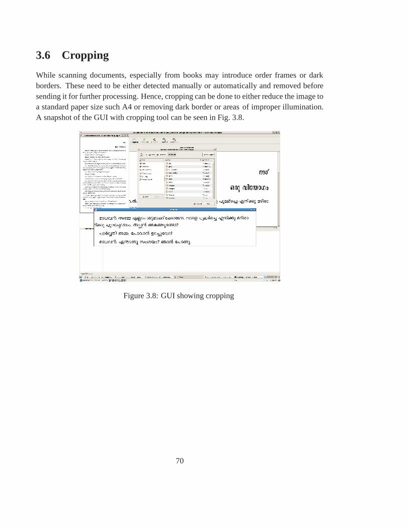
3.6 Cropping
While scanning documents, especially from books may introduce order frames or darkborders. These need to be either detected manually or automatically and removed beforesending it for further processing. Hence, cropping can be done to either reduce the image toa standard paper size such A4 or removing dark border or areasof improper illumination.A snapshot of the GUI with cropping tool can be seen in Fig. 3.8.
Figure 3.8: GUI showing cropping
70
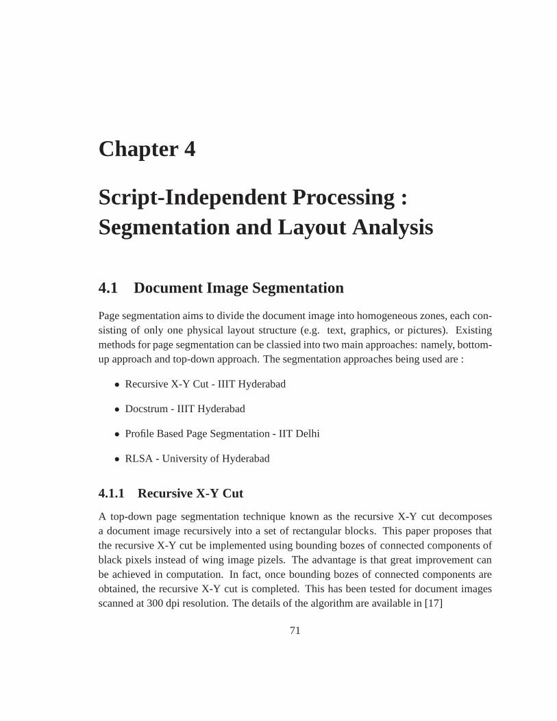
Chapter 4
Script-Independent Processing :Segmentation and Layout Analysis
4.1 Document Image Segmentation
Page segmentation aims to divide the document image into homogeneous zones, each con-sisting of only one physical layout structure (e.g. text, graphics, or pictures). Existingmethods for page segmentation can be classied into two main approaches: namely, bottom-up approach and top-down approach. The segmentation approaches being used are :
• Recursive X-Y Cut - IIIT Hyderabad
• Docstrum - IIIT Hyderabad
• Profile Based Page Segmentation - IIT Delhi
• RLSA - University of Hyderabad
4.1.1 Recursive X-Y Cut
A top-down page segmentation technique known as the recursive X-Y cut decomposesa document image recursively into a set of rectangular blocks. This paper proposes thatthe recursive X-Y cut be implemented using bounding bozes ofconnected components ofblack pixels instead of wing image pizels. The advantage is that great improvement canbe achieved in computation. In fact, once bounding bozes of connected components areobtained, the recursive X-Y cut is completed. This has been tested for document imagesscanned at 300 dpi resolution. The details of the algorithm are available in [17]
71
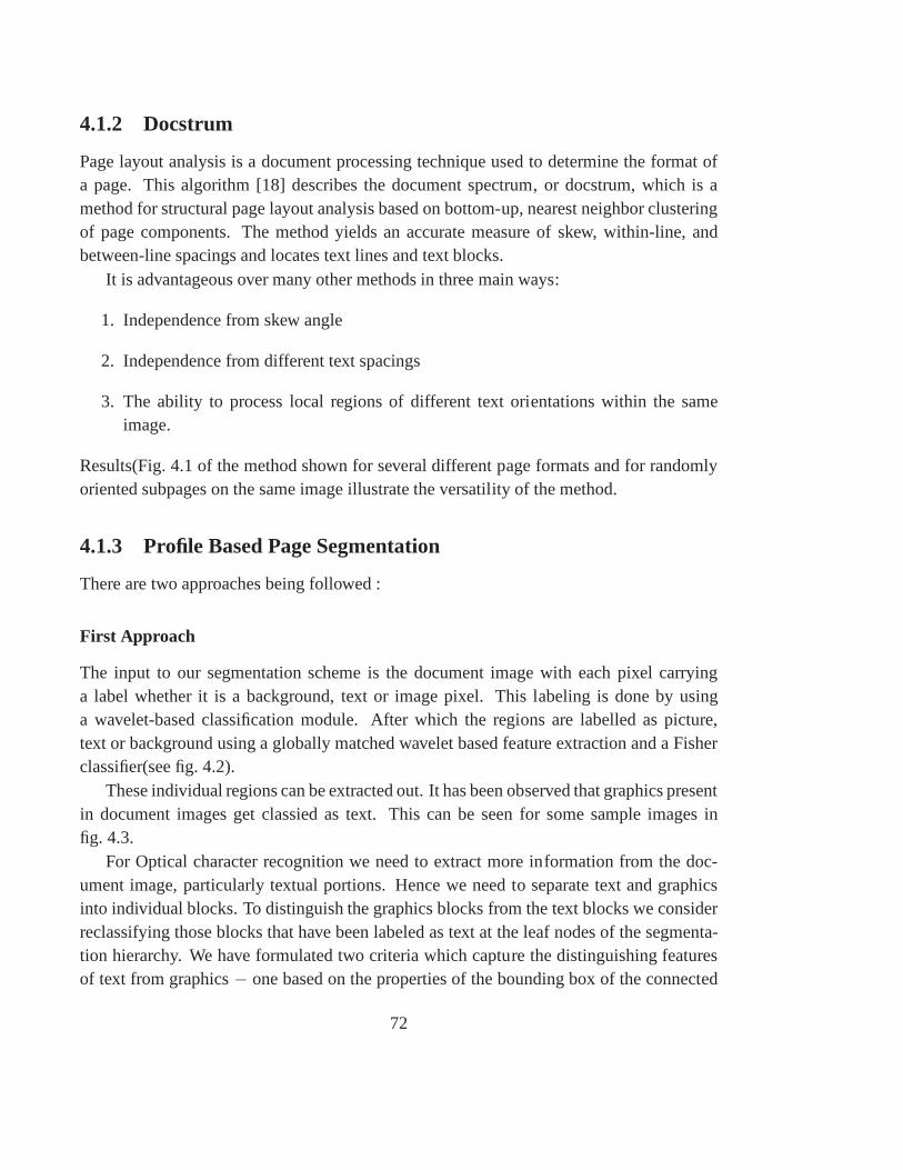
4.1.2 Docstrum
Page layout analysis is a document processing technique used to determine the format ofa page. This algorithm [18] describes the document spectrum, or docstrum, which is amethod for structural page layout analysis based on bottom-up, nearest neighbor clusteringof page components. The method yields an accurate measure ofskew, within-line, andbetween-line spacings and locates text lines and text blocks.
It is advantageous over many other methods in three main ways:
1. Independence from skew angle
2. Independence from different text spacings
3. The ability to process local regions of different text orientations within the sameimage.
Results(Fig. 4.1 of the method shown for several different page formats and for randomlyoriented subpages on the same image illustrate the versatility of the method.
4.1.3 Profile Based Page Segmentation
There are two approaches being followed :
First Approach
The input to our segmentation scheme is the document image with each pixel carryinga label whether it is a background, text or image pixel. This labeling is done by usinga wavelet-based classification module. After which the regions are labelled as picture,text or background using a globally matched wavelet based feature extraction and a Fisherclassifier(see fig. 4.2).
These individual regions can be extracted out. It has been observed that graphics presentin document images get classied as text. This can be seen for some sample images infig. 4.3.
For Optical character recognition we need to extract more information from the doc-ument image, particularly textual portions. Hence we need to separate text and graphicsinto individual blocks. To distinguish the graphics blocksfrom the text blocks we considerreclassifying those blocks that have been labeled as text atthe leaf nodes of the segmenta-tion hierarchy. We have formulated two criteria which capture the distinguishing featuresof text from graphics− one based on the properties of the bounding box of the connected
72
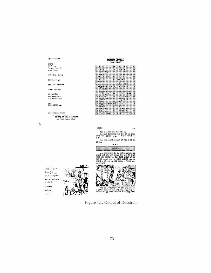
!h
Figure 4.1: Output of Docstrum
73
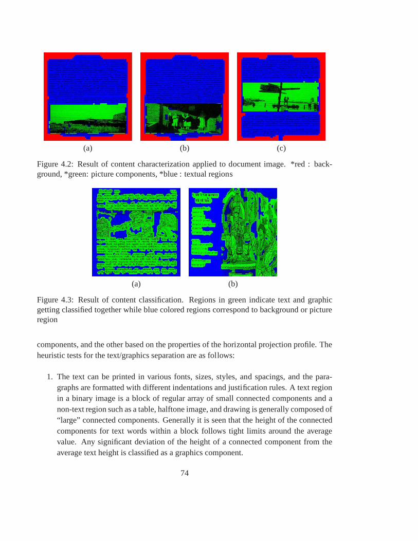
(a) (b) (c)
Figure 4.2: Result of content characterization applied to document image. *red : back-ground, *green: picture components, *blue : textual regions
(a) (b)
Figure 4.3: Result of content classification. Regions in green indicate text and graphicgetting classified together while blue colored regions correspond to background or pictureregion
components, and the other based on the properties of the horizontal projection profile. Theheuristic tests for the text/graphics separation are as follows:
1. The text can be printed in various fonts, sizes, styles, and spacings, and the para-graphs are formatted with different indentations and justification rules. A text regionin a binary image is a block of regular array of small connected components and anon-text region such as a table, halftone image, and drawingis generally composed of“large” connected components. Generally it is seen that theheight of the connectedcomponents for text words within a block follows tight limits around the averagevalue. Any significant deviation of the height of a connectedcomponent from theaverage text height is classified as a graphics component.
74
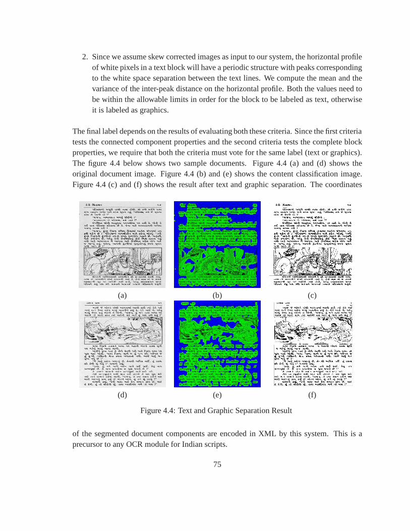
2. Since we assume skew corrected images as input to our system, the horizontal profileof white pixels in a text block will have a periodic structurewith peaks correspondingto the white space separation between the text lines. We compute the mean and thevariance of the inter-peak distance on the horizontal profile. Both the values need tobe within the allowable limits in order for the block to be labeled as text, otherwiseit is labeled as graphics.
The final label depends on the results of evaluating both these criteria. Since the first criteriatests the connected component properties and the second criteria tests the complete blockproperties, we require that both the criteria must vote for the same label (text or graphics).The figure 4.4 below shows two sample documents. Figure 4.4 (a) and (d) shows theoriginal document image. Figure 4.4 (b) and (e) shows the content classification image.Figure 4.4 (c) and (f) shows the result after text and graphicseparation. The coordinates
(a) (b) (c)
(d) (e) (f)
Figure 4.4: Text and Graphic Separation Result
of the segmented document components are encoded in XML by this system. This is aprecursor to any OCR module for Indian scripts.
75
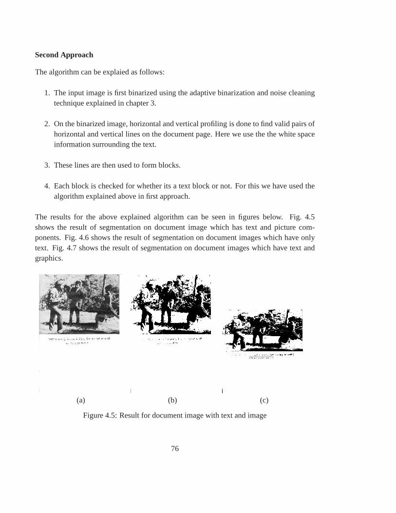
Second Approach
The algorithm can be explaied as follows:
1. The input image is first binarized using the adaptive binarization and noise cleaningtechnique explained in chapter 3.
2. On the binarized image, horizontal and vertical profilingis done to find valid pairs ofhorizontal and vertical lines on the document page. Here we use the the white spaceinformation surrounding the text.
3. These lines are then used to form blocks.
4. Each block is checked for whether its a text block or not. For this we have used thealgorithm explained above in first approach.
The results for the above explained algorithm can be seen in figures below. Fig. 4.5shows the result of segmentation on document image which hastext and picture com-ponents. Fig. 4.6 shows the result of segmentation on document images which have onlytext. Fig. 4.7 shows the result of segmentation on document images which have text andgraphics.
(a) (b) (c)
Figure 4.5: Result for document image with text and image
76
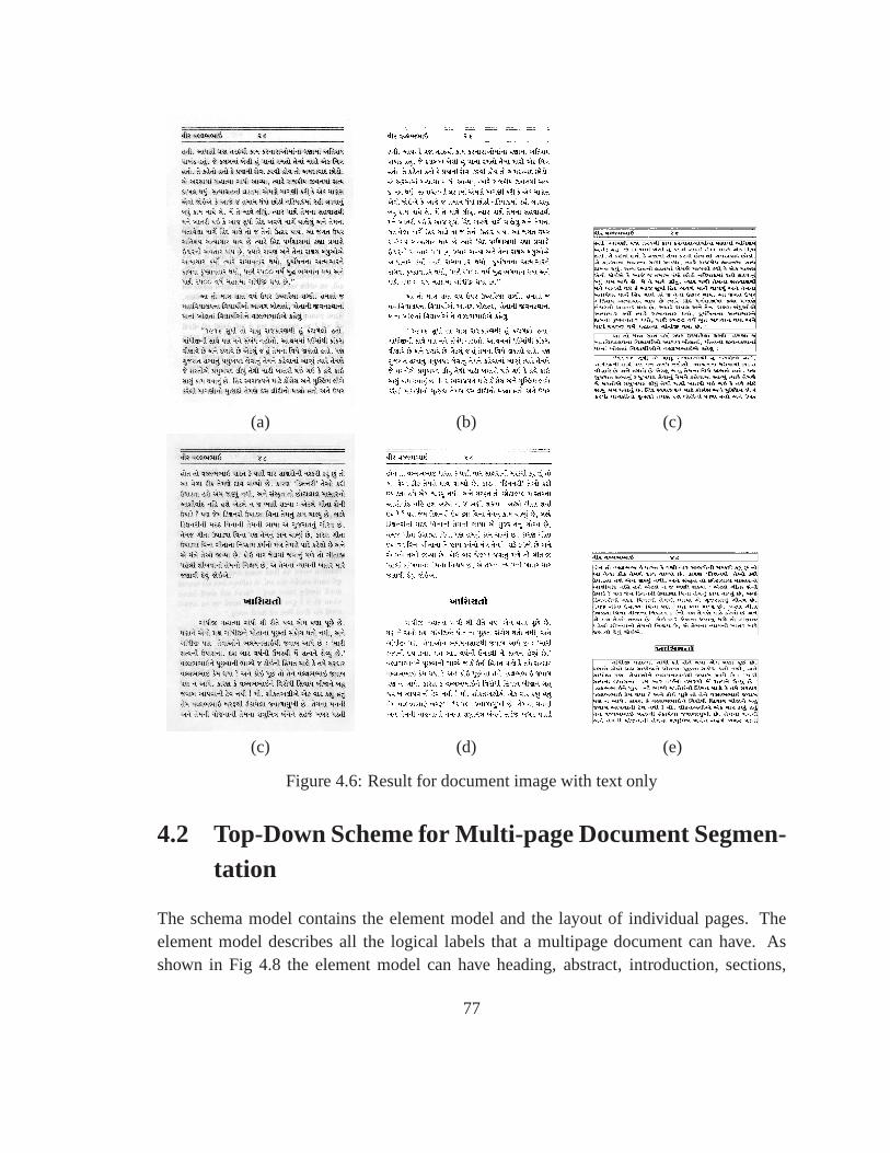
(a) (b) (c)
(c) (d) (e)
Figure 4.6: Result for document image with text only
4.2 Top-Down Scheme for Multi-page Document Segmen-tation
The schema model contains the element model and the layout ofindividual pages. Theelement model describes all the logical labels that a multipage document can have. Asshown in Fig 4.8 the element model can have heading, abstract, introduction, sections,
77
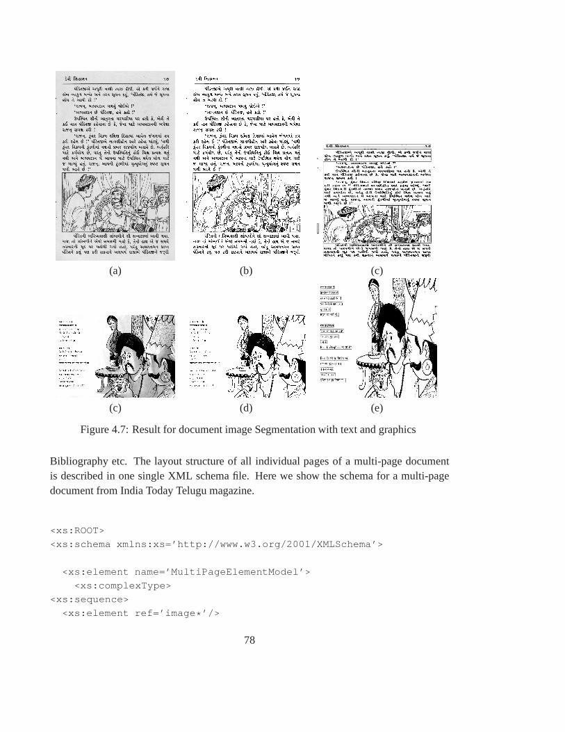
(a) (b) (c)
(c) (d) (e)
Figure 4.7: Result for document image Segmentation with text and graphics
Bibliography etc. The layout structure of all individual pages of a multi-page documentis described in one single XML schema file. Here we show the schema for a multi-pagedocument from India Today Telugu magazine.
<xs:ROOT>
<xs:schema xmlns:xs=’http://www.w3.org/2001/XMLSchema’>
<xs:element name=’MultiPageElementModel’>
<xs:complexType>
<xs:sequence>
<xs:element ref=’image*’/>
78
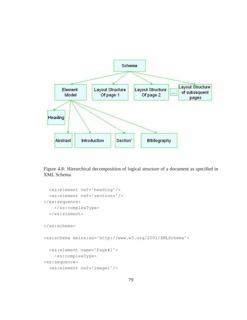
Figure 4.8: Hierarchical decomposition of logical structure of a document as specified inXML Schema
<xs:element ref=’heading’/>
<xs:element ref=’section*’/>
</xs:sequence>
</xs:complexType>
</xs:element>
</xs:schema>
<xs:schema xmlns:xs=’http://www.w3.org/2001/XMLSchema’>
<xs:element name=’Page#1’>
<xs:complexType>
<xs:sequence>
<xs:element ref=’image1’/>
79
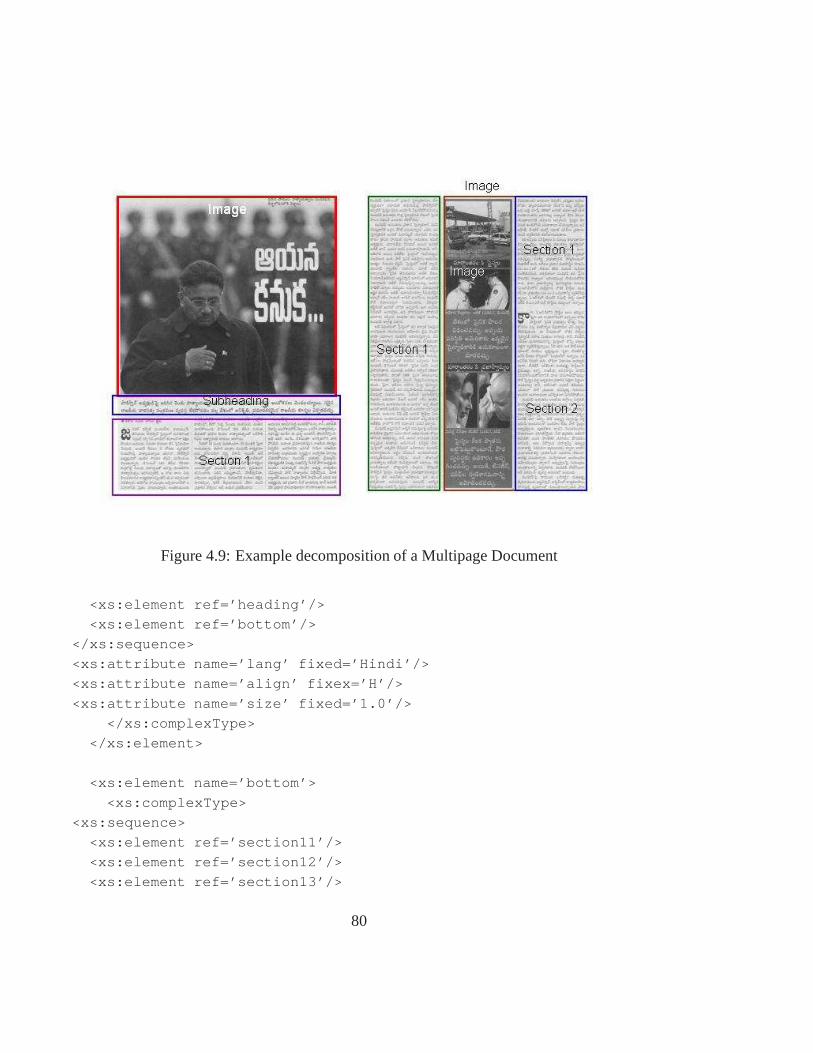
Figure 4.9: Example decomposition of a Multipage Document
<xs:element ref=’heading’/>
<xs:element ref=’bottom’/>
</xs:sequence>
<xs:attribute name=’lang’ fixed=’Hindi’/>
<xs:attribute name=’align’ fixex=’H’/>
<xs:attribute name=’size’ fixed=’1.0’/>
</xs:complexType>
</xs:element>
<xs:element name=’bottom’>
<xs:complexType>
<xs:sequence>
<xs:element ref=’section11’/>
<xs:element ref=’section12’/>
<xs:element ref=’section13’/>
80
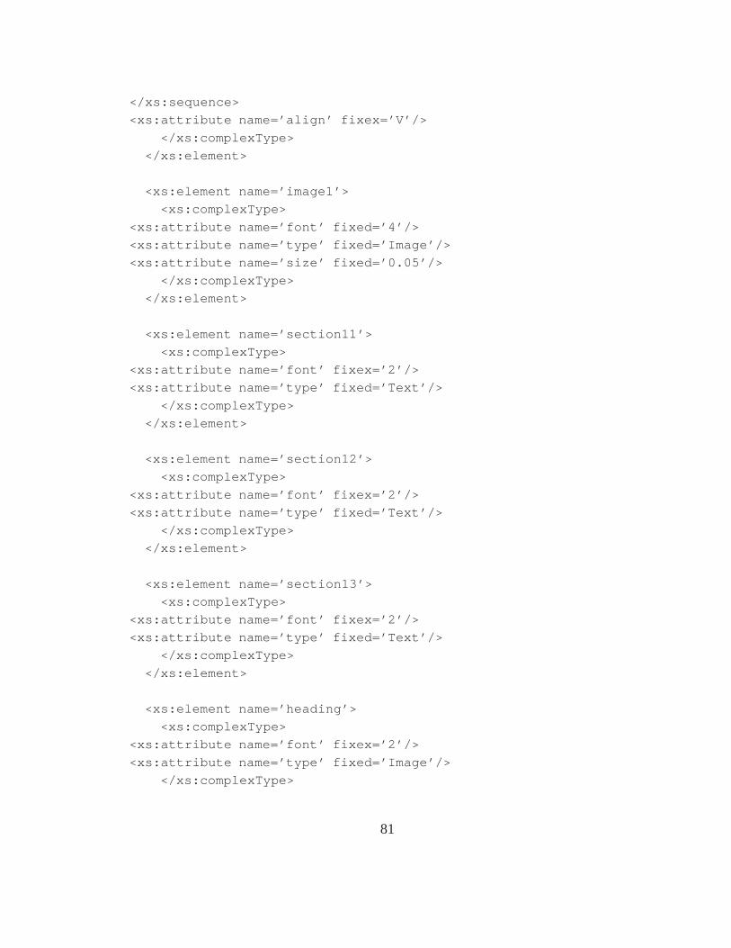
</xs:sequence>
<xs:attribute name=’align’ fixex=’V’/>
</xs:complexType>
</xs:element>
<xs:element name=’image1’>
<xs:complexType>
<xs:attribute name=’font’ fixed=’4’/>
<xs:attribute name=’type’ fixed=’Image’/>
<xs:attribute name=’size’ fixed=’0.05’/>
</xs:complexType>
</xs:element>
<xs:element name=’section11’>
<xs:complexType>
<xs:attribute name=’font’ fixex=’2’/>
<xs:attribute name=’type’ fixed=’Text’/>
</xs:complexType>
</xs:element>
<xs:element name=’section12’>
<xs:complexType>
<xs:attribute name=’font’ fixex=’2’/>
<xs:attribute name=’type’ fixed=’Text’/>
</xs:complexType>
</xs:element>
<xs:element name=’section13’>
<xs:complexType>
<xs:attribute name=’font’ fixex=’2’/>
<xs:attribute name=’type’ fixed=’Text’/>
</xs:complexType>
</xs:element>
<xs:element name=’heading’>
<xs:complexType>
<xs:attribute name=’font’ fixex=’2’/>
<xs:attribute name=’type’ fixed=’Image’/>
</xs:complexType>
81
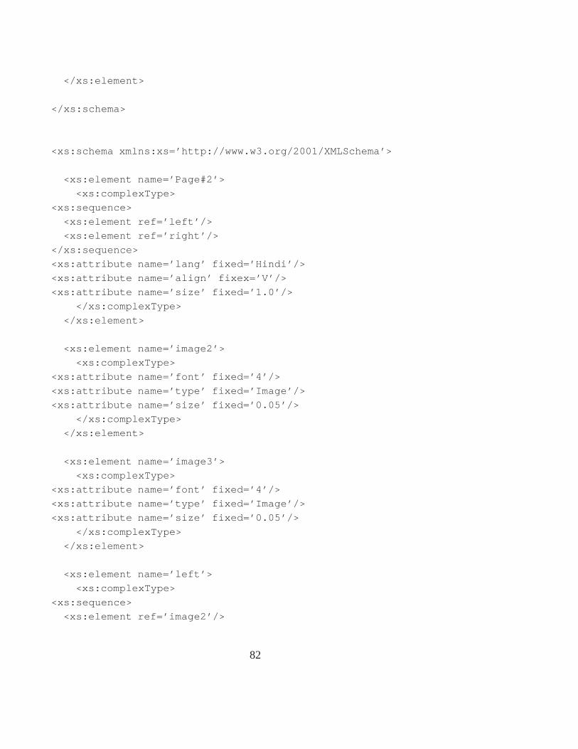
</xs:element>
</xs:schema>
<xs:schema xmlns:xs=’http://www.w3.org/2001/XMLSchema’>
<xs:element name=’Page#2’>
<xs:complexType>
<xs:sequence>
<xs:element ref=’left’/>
<xs:element ref=’right’/>
</xs:sequence>
<xs:attribute name=’lang’ fixed=’Hindi’/>
<xs:attribute name=’align’ fixex=’V’/>
<xs:attribute name=’size’ fixed=’1.0’/>
</xs:complexType>
</xs:element>
<xs:element name=’image2’>
<xs:complexType>
<xs:attribute name=’font’ fixed=’4’/>
<xs:attribute name=’type’ fixed=’Image’/>
<xs:attribute name=’size’ fixed=’0.05’/>
</xs:complexType>
</xs:element>
<xs:element name=’image3’>
<xs:complexType>
<xs:attribute name=’font’ fixed=’4’/>
<xs:attribute name=’type’ fixed=’Image’/>
<xs:attribute name=’size’ fixed=’0.05’/>
</xs:complexType>
</xs:element>
<xs:element name=’left’>
<xs:complexType>
<xs:sequence>
<xs:element ref=’image2’/>
82
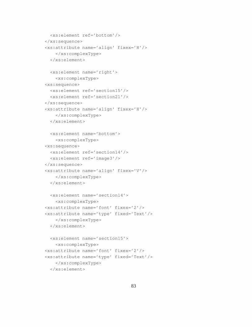
<xs:element ref=’bottom’/>
</xs:sequence>
<xs:attribute name=’align’ fixex=’H’/>
</xs:complexType>
</xs:element>
<xs:element name=’right’>
<xs:complexType>
<xs:sequence>
<xs:element ref=’section15’/>
<xs:element ref=’section21’/>
</xs:sequence>
<xs:attribute name=’align’ fixex=’H’/>
</xs:complexType>
</xs:element>
<xs:element name=’bottom’>
<xs:complexType>
<xs:sequence>
<xs:element ref=’section14’/>
<xs:element ref=’image3’/>
</xs:sequence>
<xs:attribute name=’align’ fixex=’V’/>
</xs:complexType>
</xs:element>
<xs:element name=’section14’>
<xs:complexType>
<xs:attribute name=’font’ fixex=’2’/>
<xs:attribute name=’type’ fixed=’Text’/>
</xs:complexType>
</xs:element>
<xs:element name=’section15’>
<xs:complexType>
<xs:attribute name=’font’ fixex=’2’/>
<xs:attribute name=’type’ fixed=’Text’/>
</xs:complexType>
</xs:element>
83

<xs:element name=’section21’>
<xs:complexType>
<xs:attribute name=’font’ fixex=’2’/>
<xs:attribute name=’type’ fixed=’Text’/>
</xs:complexType>
</xs:element>
</xs:schema>
</xs:ROOT>
This is an example of a document class where the page has got a fixed layout, i.e. therelative position of every element is fixed and hence the alignment information of childelements within the parent element can be used to obtain the page layout. The alignmentinformation is specified in the attribute list of the parent element. There are several at-tributes specified for an element but the attribute of interest to the segmentation moduleare:
• align : whose allowed values are H (Horizontal), V (Vertical) or R (Random). Ran-dom alignment is specified when the child elements are randomly placed within theparent element. For example, in a newspaper page, the news articles are of varyingsizes and aligned in a random way.
• type : whose value in quotes can beTextor Imagewhich means that the element hastext content or image content respectively. It has been observed that many a times,large font sized text is mis-identified as image by the content identification module.In order to ensure that the final labelling of blocks does not go wrong because ofthis possible mis-identification, another value fortypeattribute has been used viz.TextImagewhich means that the element can be identified as text or image.
• font : whose value in quotes is the font size of the text content. The font size need notbe the actual one since the segmentation module will be mainly concerned with therelative font sizes of the elements. For example, the font size specified for headingshould be larger than that of the text which follows.
Some other attributes used are :
• lang : The value of this attribute specifies the language of the root element, which isthe entire document page itself.
84
• size: This attribute specifies the relative area of the child element within the parentelement. Though this information is of no interest to the segmentation module, itis used by the software which displays the schema on the document page. If thealignment of child elements in the parent element is random,the size informationconveys no sense and hence, such schemas cannot be displayedon the documentpage.
4.2.1 Top-down Segmentation using Document Schema
The document class specific schema model contains information about the layout structureof the elements in a top down manner. An element at a higher level of hierarchy is calledParent elementand its constituent smaller elements are calledChild elements. Going bythe structure given in the schema, the segmentation module tries to identify regions in thedocument page starting from the root element and going down the hierarchy, possibly intel-ligently clustering the smaller blocks constructed by the bottom-up segmentation approachbased on the content information of child elements as specified in the schema. Given thecontent-model of the parent element and the parent block dimensions, we need to iden-tify the child element blocks within it using the information provided in the schema. Weillustrate the strategy followed when the alignment is horizontal.
The child elements are identified in order, from topmost to bottom-most. The blockwhich has to be identified will have only one unknown edge, thebottom-most, since theleftmost edge and the rightmost edge follow that of the parent block and the topmost edgefollows either the parent block’s topmost edge or the previously identified child block’sbottom-most edge. The goal is to locate the unknown edge which is the dividing linebetween two types of child elements whose content informations are there in the schema.
Depending on the content information of the elements on either side of the unknownedge (line), it is possible to predict about theexpected regionwhere the horizontal dividingline is to be searched. For example, if the first region is having text-only content and theother region is having images with text aligned on the right side (this case arises when thedividing line betweenContentLabelelement andContentselement is to be detected in theSpectrum magazinecontentpage), a search is made for all the images, with text on the rightside, in theunlabeledregion of the parent block and the top edge of the topmost image isconsidered as the lower bound of theexpected region. Since the first region is having text-only content, all the blocks within the parent block whose top edge touches the top edge ofthe first element are identified and the lower-most edge of allthese blocks is considered asthe top bound of theexpected region. Similar heuristics have been designed to locate theexpected regionin other cases by exploiting the distinguishing features about the contents
85
e.g. presence of image(s), image alignment, font sizes of texts, relative placement of textblocks of different font sizes etc.
Once theexpected regionhas been identified, all the horizontal lines (possible dividinglines) which run across the entire parent block are searched. Each such line is then subjectedto a confirmation test, in which the blocks lying on either side of the candidate line arechecked for their contents and relative positions to confirmif they comply with th schemaspecifications. The line which complies best with schema specifications is selected. Theselected line’s position is taken as the unknown edge (the lower edge). Once the boundaryof this child element have been ascertained, it becomes the upper edge of the next childelement, which is aligned horizontally with it. Continuingthis way, the identify the regionsof other child elements.
An analogous procedure is used to detect the child elements if the alignment isvertical.However, in the case of random alignment of the child elements within the parent element,the layout of the child elements is not known, but the schema specifies the contents of thechild elements. Based on this content information, detection and grouping of blocks whichcomply with the schema information is carried out.
4.3 Content Classification
we propose a novel scheme for text extraction using matched wavelet filters [?]. Themethod does not require any a priori information about the font type, font size, font orienta-tion, geometric distortion or background texture because we have used matched wavelets tocapture textural characteristics of image regions. Clustering based approach has been pro-posed for estimating globally matched wavelets (GMWs) froma collection of groundtruthedimages. Any general image can be categorized as either a scene image or document im-age. But in a document image we can further classify the non text part as either imageor background. Segmentation of document image into these three classes is necessary forassociating detailed physical and semantic properties with the documents. Fisher classi-fiers have been used for this purpose and we further exploit the contextual information viaMRF formulation to refine the results. Potts interaction penalty, considered to be one of thesimplest discontinuity preserving energy function, has been used in the MRF modelling.
4.3.1 Estimating Globally Matched Wavelet filters
Motivation for the use of matched wavelet filters for text extraction comes from the factthat wavelet filters matched to a particular signal minimizethe energy of that signal flowingin the detail (wavelet) space. At an abstract level our system use a set of trained wavelet
86
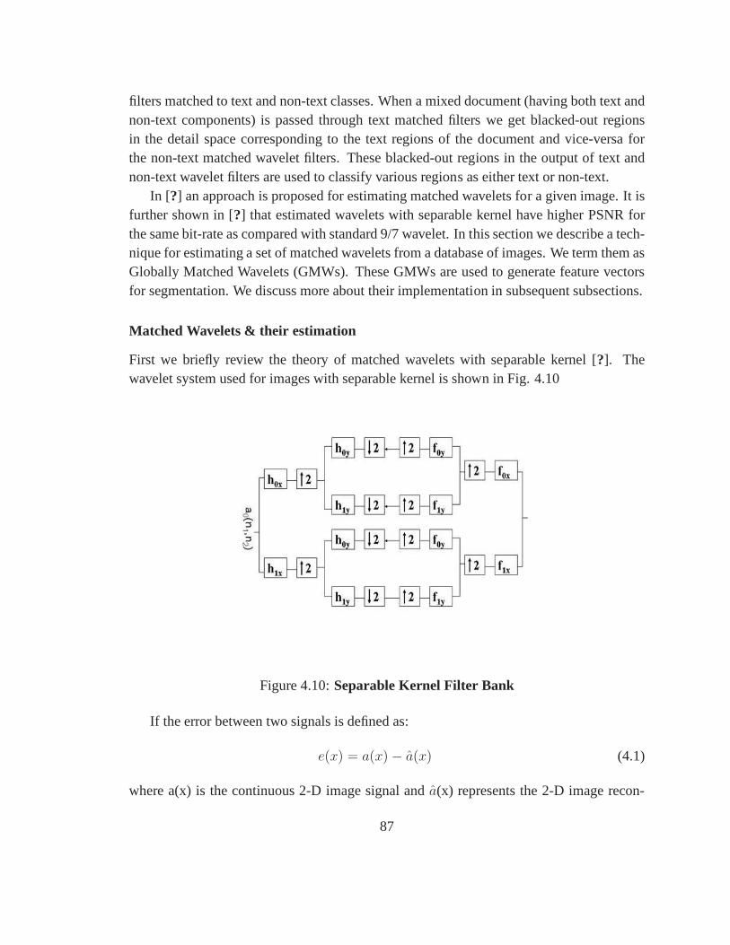
filters matched to text and non-text classes. When a mixed document (having both text andnon-text components) is passed through text matched filterswe get blacked-out regionsin the detail space corresponding to the text regions of the document and vice-versa forthe non-text matched wavelet filters. These blacked-out regions in the output of text andnon-text wavelet filters are used to classify various regions as either text or non-text.
In [?] an approach is proposed for estimating matched wavelets for a given image. It isfurther shown in [?] that estimated wavelets with separable kernel have higherPSNR forthe same bit-rate as compared with standard 9/7 wavelet. In this section we describe a tech-nique for estimating a set of matched wavelets from a database of images. We term them asGlobally Matched Wavelets (GMWs). These GMWs are used to generate feature vectorsfor segmentation. We discuss more about their implementation in subsequent subsections.
Matched Wavelets & their estimation
First we briefly review the theory of matched wavelets with separable kernel [?]. Thewavelet system used for images with separable kernel is shown in Fig. 4.10
Figure 4.10:Separable Kernel Filter Bank
If the error between two signals is defined as:
e(x) = a(x)− a(x) (4.1)
where a(x) is the continuous 2-D image signal anda(x) represents the 2-D image recon-
87
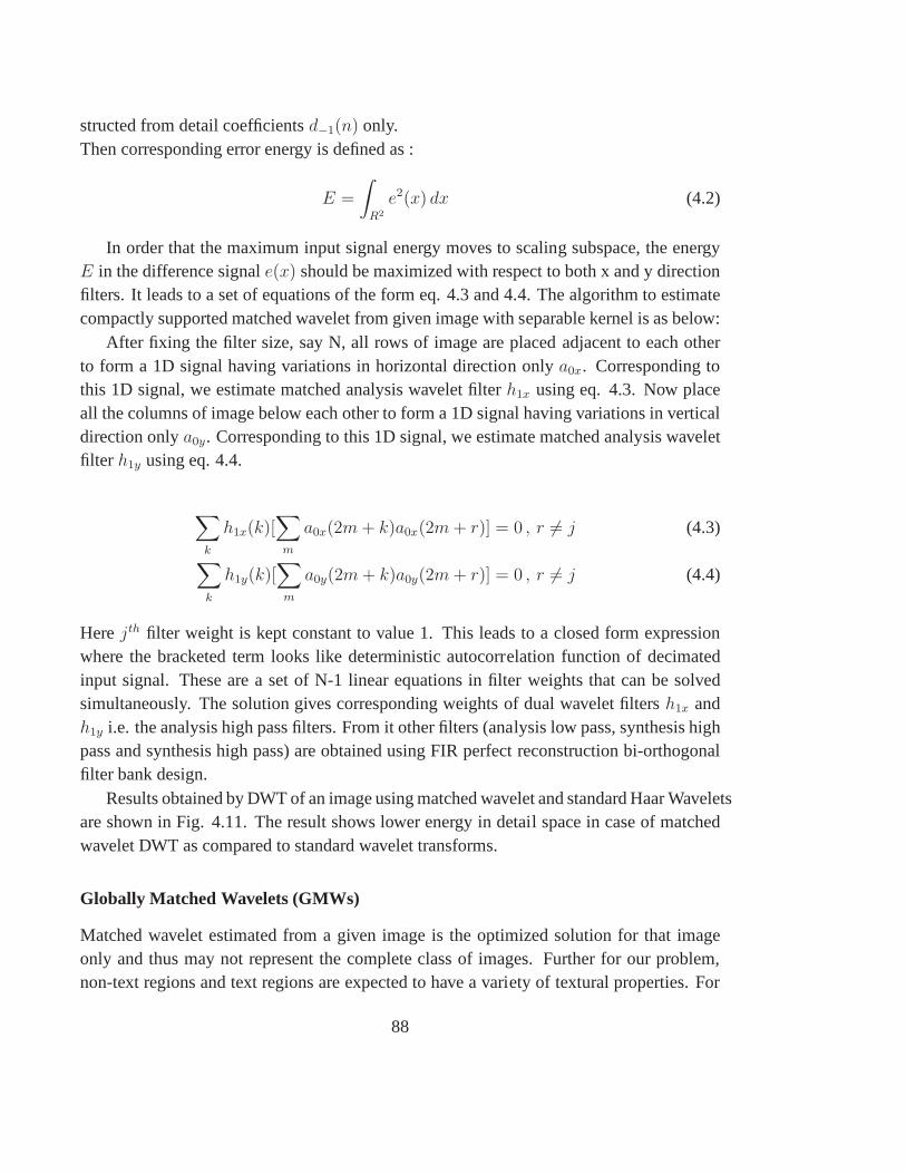
structed from detail coefficientsd−1(n) only.Then corresponding error energy is defined as :
E =
∫
R2
e2(x) dx (4.2)
In order that the maximum input signal energy moves to scaling subspace, the energyE in the difference signale(x) should be maximized with respect to both x and y directionfilters. It leads to a set of equations of the form eq. 4.3 and 4.4. The algorithm to estimatecompactly supported matched wavelet from given image with separable kernel is as below:
After fixing the filter size, say N, all rows of image are placedadjacent to each otherto form a 1D signal having variations in horizontal direction only a0x. Corresponding tothis 1D signal, we estimate matched analysis wavelet filterh1x using eq. 4.3. Now placeall the columns of image below each other to form a 1D signal having variations in verticaldirection onlya0y. Corresponding to this 1D signal, we estimate matched analysis waveletfilter h1y using eq. 4.4.
∑
k
h1x(k)[∑
m
a0x(2m + k)a0x(2m + r)] = 0 , r 6= j (4.3)
∑
k
h1y(k)[∑
m
a0y(2m + k)a0y(2m + r)] = 0 , r 6= j (4.4)
Herejth filter weight is kept constant to value 1. This leads to a closed form expressionwhere the bracketed term looks like deterministic autocorrelation function of decimatedinput signal. These are a set of N-1 linear equations in filterweights that can be solvedsimultaneously. The solution gives corresponding weightsof dual wavelet filtersh1x andh1y i.e. the analysis high pass filters. From it other filters (analysis low pass, synthesis highpass and synthesis high pass) are obtained using FIR perfectreconstruction bi-orthogonalfilter bank design.
Results obtained by DWT of an image using matched wavelet andstandard Haar Waveletsare shown in Fig. 4.11. The result shows lower energy in detail space in case of matchedwavelet DWT as compared to standard wavelet transforms.
Globally Matched Wavelets (GMWs)
Matched wavelet estimated from a given image is the optimized solution for that imageonly and thus may not represent the complete class of images.Further for our problem,non-text regions and text regions are expected to have a variety of textural properties. For
88
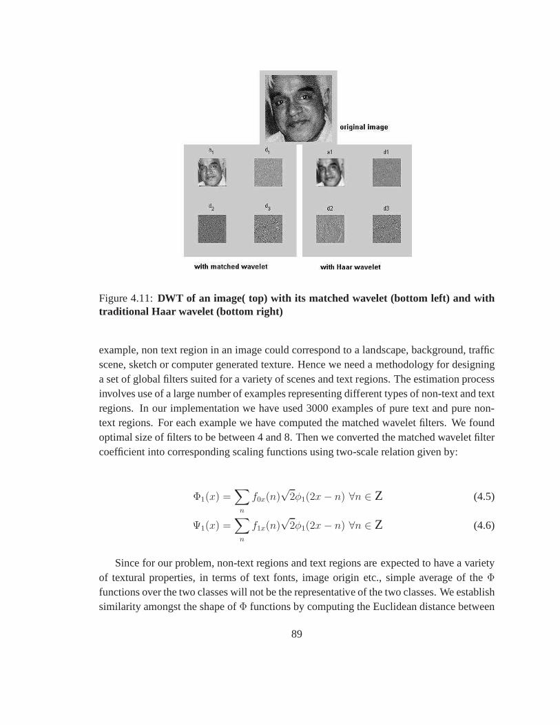
Figure 4.11:DWT of an image( top) with its matched wavelet (bottom left) and withtraditional Haar wavelet (bottom right)
example, non text region in an image could correspond to a landscape, background, trafficscene, sketch or computer generated texture. Hence we need amethodology for designinga set of global filters suited for a variety of scenes and text regions. The estimation processinvolves use of a large number of examples representing different types of non-text and textregions. In our implementation we have used 3000 examples ofpure text and pure non-text regions. For each example we have computed the matched wavelet filters. We foundoptimal size of filters to be between 4 and 8. Then we convertedthe matched wavelet filtercoefficient into corresponding scaling functions using two-scale relation given by:
Φ1(x) =∑
n
f0x(n)√
2φ1(2x− n) ∀n ∈ Z (4.5)
Ψ1(x) =∑
n
f1x(n)√
2φ1(2x− n) ∀n ∈ Z (4.6)
Since for our problem, non-text regions and text regions areexpected to have a varietyof textural properties, in terms of text fonts, image originetc., simple average of theΦfunctions over the two classes will not be the representative of the two classes. We establishsimilarity amongst the shape ofΦ functions by computing the Euclidean distance between
89
their sampled values. Depending upon this similarity measure, Φ functions are groupedinto homogeneous clusters using a modified iso-data algorithm. Homogenous clusters arethose clusters which containΦ functions matched to regions of a single type only (text orimage). In the present implementation of the iso-data algorithm we start with two clustersand increase the number of clusters if
∃ i s.t. ri > thresmin or ri < thresmax
whereri=C1i/C2i, Cci= number of data points in cluster i which are coming from classc.
Using iso-data clustering ensures that final clusters are dominated by either image ortext samples. Thus they are expected to be representative ofeither the text or non-textclasses. For each cluster Globally Matched wavelet filter coefficients are computed byfinding there respective cluster centers. Being cluster centers, GMWs are the measure ofaverage shape given by following formula
GKk(m) =1
nk
nk∑
i
Xki (m) 0 ≤ m ≤ NΦ (4.7)
WhereGXk(m) is themth element ofkth GMW. Xki (n) representsnth coefficient of
kth image of the cluster. Next we discuss a GMW based text detection scheme.
4.3.2 Locating text from arbitrary backgrounds
Because of extensive training GMW based algorithm can detect text regions in a variety ofsituations of text deformations, different fonts and scales. The following subsections givethe detail algorithm for this purpose.
Algorithm
Globally Matched Wavelets (GMWs) are the characteristic wavelets of pure non-text andtext classes. We have GMW filters corresponding to the GMWs obtained in the previoussection using the two scale relation. Table 4.1 shows the 12 (6 each in x and y direction)high pass analysis GMW filters obtained.
To locate text regions in an image, I(n1,n2), pass the image through wavelet analysisfilter bank (Fig. 4.10), with each of 6 GMW filter sets to obtain6 transformed images.The matched wavelet is found with the intention that the maximum energy goes into theapproximation sub-space. If we pass a text image through thefilter bank consisting of
90
GMW filters of text then we get minimum energy in the detail sub-space. On the otherhand if a pure image is passed through this filter bank then we get considerable energygoing into detail sub-space. So when we pass a typical mixed image through a GMW oftext we get pure image regions dominant in detail sub-space.Similarly when we pass atypical mixed image through a GMW of pure image, we get text regions dominant in detailsub-space.
In order to enhance this information we use Standard Deviation (SD) which is nothingbut the local energy of each pixel. It is followed by Gaussianfiltering to minimize effect ofisolated noise from the transformed images [?]. We calculate the local standard deviationof each pixel in transformed image using
engki(x, y) =
√
√
√
√
1
R
w∑
m=1
w∑
n=1
∣
∣(hki(m, n)2 − hki
(m, n)2)∣
∣
wherew(= 9) is the window size andR = w ∗ w, while hki(x, y) is the mean around
the(x, y)th pixel andhki(x, y) is the filtered image. Following this, the Gaussian Filtering
is done using:
Featki(x, y) =
1
G2
∑
(m,n)∈Gx,y
|engki(m, n)|
whereGx,y is theG∗G gaussian smoothing window andFeatkiis the final transformed
6 dimensional feature image. Thus at the end of it we have a stack of 6 transformed images.We define our feature vector at each pixel as
f(x, y) = [f1(x, y), f2(x, y), f3(x, y), f4(x, y), f5(x, y), f6(x, y)]
Wherefi(x,y) is the value of pixel(x,y) of transformed imagei.
4.3.3 Classification
Having obtained the feature vectors, for classification of pixels as either text or non-text wehave used two different schemes: segregation of test image pixels into two classes usingk-means algorithm followed by class assignment based on result of SVM trained on theratio of cluster centers and Fisher Classifiers. An ideal classification approach may have a
91
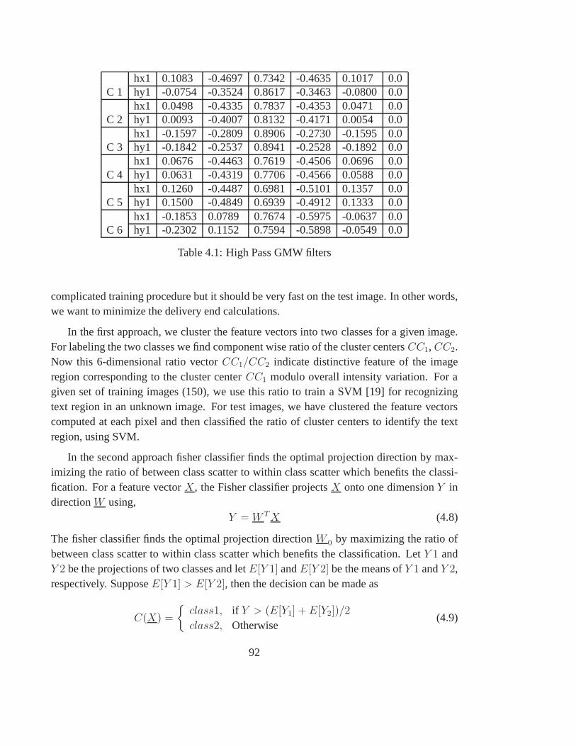
hx1 0.1083 -0.4697 0.7342 -0.4635 0.1017 0.0C 1 hy1 -0.0754 -0.3524 0.8617 -0.3463 -0.0800 0.0
hx1 0.0498 -0.4335 0.7837 -0.4353 0.0471 0.0C 2 hy1 0.0093 -0.4007 0.8132 -0.4171 0.0054 0.0
hx1 -0.1597 -0.2809 0.8906 -0.2730 -0.1595 0.0C 3 hy1 -0.1842 -0.2537 0.8941 -0.2528 -0.1892 0.0
hx1 0.0676 -0.4463 0.7619 -0.4506 0.0696 0.0C 4 hy1 0.0631 -0.4319 0.7706 -0.4566 0.0588 0.0
hx1 0.1260 -0.4487 0.6981 -0.5101 0.1357 0.0C 5 hy1 0.1500 -0.4849 0.6939 -0.4912 0.1333 0.0
hx1 -0.1853 0.0789 0.7674 -0.5975 -0.0637 0.0C 6 hy1 -0.2302 0.1152 0.7594 -0.5898 -0.0549 0.0
Table 4.1: High Pass GMW filters
complicated training procedure but it should be very fast onthe test image. In other words,we want to minimize the delivery end calculations.
In the first approach, we cluster the feature vectors into twoclasses for a given image.For labeling the two classes we find component wise ratio of the cluster centersCC1, CC2.Now this 6-dimensional ratio vectorCC1/CC2 indicate distinctive feature of the imageregion corresponding to the cluster centerCC1 modulo overall intensity variation. For agiven set of training images (150), we use this ratio to traina SVM [19] for recognizingtext region in an unknown image. For test images, we have clustered the feature vectorscomputed at each pixel and then classified the ratio of cluster centers to identify the textregion, using SVM.
In the second approach fisher classifier finds the optimal projection direction by max-imizing the ratio of between class scatter to within class scatter which benefits the classi-fication. For a feature vectorX, the Fisher classifier projectsX onto one dimensionY indirectionW using,
Y = W T X (4.8)
The fisher classifier finds the optimal projection directionW 0 by maximizing the ratio ofbetween class scatter to within class scatter which benefitsthe classification. LetY 1 andY 2 be the projections of two classes and letE[Y 1] andE[Y 2] be the means ofY 1 andY 2,respectively. SupposeE[Y 1] > E[Y 2], then the decision can be made as
C(X) =
{
class1, if Y > (E[Y1] + E[Y2])/2
class2, Otherwise(4.9)
92
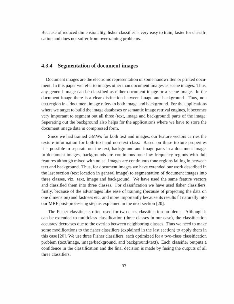
Because of reduced dimensionality, fisher classifier is veryeasy to train, faster for classifi-cation and does not suffer from overtraining problems.
4.3.4 Segmentation of document images
Document images are the electronic representation of some handwritten or printed docu-ment. In this paper we refer to images other than document images as scene images. Thus,any general image can be classified as either document image or a scene image. In thedocument image there is a clear distinction between image and background. Thus, nontext region in a document image refers to both image and background. For the applicationswhere we target to build the image databases or semantic image retrival engines, it becomesvery important to segment out all three (text, image and background) parts of the image.Seperating out the background also helps for the applications where we have to store thedocument image data in compressed form.
Since we had trained GMWs for both text and images, our feature vectors carries thetexture information for both text and non-text class. Basedon these texture propertiesit is possible to separate out the text, background and imageparts in a document image.In document images, backgrounds are continuous tone low frequency regions with dullfeatures although mixed with noise. Images are continuous tone regions falling in betweentext and background. Thus, for document images we have extended our work described inthe last section (text location in general image) to segmentation of document images intothree classes, viz. text, image and background. We have usedthe same feature vectorsand classified them into three classes. For classification wehave used fisher classifiers,firstly, because of the advantages like ease of training (because of projecting the data onone dimension) and fastness etc. and more importantly because its results fit naturally intoour MRF post-processing step as explained in the next section [20].
The Fisher classifier is often used for two-class classification problems. Although itcan be extended to multiclass classification (three classesin our case), the classificationaccuracy decreases due to the overlap between neighboring classes. Thus we need to makesome modifications to the fisher classifiers (explained in thelast section) to apply them inthis case [20]. We use three Fisher classifiers, each optimized for a two-class classificationproblem (text/image, image/background, and background/text). Each classifier outputs aconfidence in the classification and the final decision is madeby fusing the outputs of allthree classifiers.
93

Classification Confidence
Let among the three classifiers, classifier 1 refers to image and background, classifier 2refers to image and text, classifier 3 refers to background and text. From the previoussection we have algorithm to evaluate theW 0 values for all the three classifiers. We usetheseW 0 values along with the groundtruthed images to find out the distribution of Y forboth the classes of each classifier. For example, in our case we obtain the distribution ofYvalues corresponding to image and background in classifier 1(represented asY1a andY1c),image and text in classifier 2 (represented asY2a andY2b), background and text in classifier3 (represented asY3c andY3b) respectively. After normalizing these distributions, weusethe curve fits to fit the higher order gaussian functions to these distributions. This provideus with the approximate pdf’s of these projections. Let us represent these distributions byfY (y). The plot of these distribution functions for classifier 1 isshown in Fig. 4.12.
Figure 4.12:Distribution of Y for Image and Background as obtained from Classifier1. Similar distributions are obtained for Classifiers 2 and 3
The classification confidenceCi,j of classi using classifierj is defined as
Ci,j =
{
fY (y/X∈classi)fY (y/X∈classi)+fY (y/X∈anotherclass)
, if i is applicable for classifier j.
0, Otherwise
wherei is the class label andj represents the trained classifiers. If a classifier is trainedto classes1 and2, its output is not applicable to estimating the classification confidence ofclass3. Therefore,C3,j = 0. In other words, for a classi, Ci,j ∈ [0, 1] for the two applicableclassifiers andCi,j = 0 for the third classifier. The final classification confidence is definedas
94
Ci =1
2
3∑
j=1
Ci,j (4.10)
Note that,Ci ∈ [0, 1], i = 1, 2, 3. However,Ci is not a good estimate of the a pos-teriori probability since
∑3i=1 Ci = 1.5 instead of1. We can takeCi as an estimate of a
nondecreasing function of the a posteriori probability, which is a kind of generalized clas-sification confidence [?]. ThusCi represents the probability of a pixel belonging to classi(= 1, 2, 3).
4.3.5 MRF postprocessing for Document Image Segmentation
Using the same text extraction features for document image segmentation may lead tooverlapping in the feature space. This is especially true for the image and backgroundclasses because of lack of hard distinction between the textures of these two classes. Wedeal with this problem by exploiting the contextual information around each pixel. Similarapproach has been used recently in [20] to refine the results of segmenting the handwrittentext, printed text and noise in the document image. Removingthis misclassification isequivalent to making the classification smoother. In this section we present MRF basedapproach for classification smoothening using context around pixels.
Figure 4.13:Document Segmentation results obtained for 2 sample imagesfrom pre-vious section. Images show that the misclassification occurs either at the class bound-aries or because of the presence of small isolated clusters.
95
MRF: Background
The problem of correcting the misclassification belongs to very general class of problems invision and can be formulated in terms of energy minimization[21]. Every pixelp must beassigned a label in the setL = {text, image, background}. F refers a particular labellingof the pixels andfp refers to the value of the label of a particular pixel. We consider thefirst order MRF model. This simplifies the energy function to the following form:
E(f) =∑
{p,q}∈N
Vp,q(fp, fq) +∑
p∈P
Dp(fp) (4.11)
whereN is the set of interacting pair of pixels. We considerN to be eight neighbour-hood of a pixel. The first and second terms in the above equation are refered to asEsmooth
(interaction energy) andEdata (energy corresponding to the data term) in the literature [21].Dp (Data Term) is the measure of how well a labelfp fits the pixelp given the observeddata. Thus in our case classification confidence found in the previous section is the intutivechoice ofDp [20].
Esmooth makesF smooth everywhere. Although smoothing is required for removingmisclassification, but oversmoothing can lead to poor results at the object boundaries. En-ergy functions that dont have this problem are refered to asDiscontinuity Preserving. Onesuch example of discontinuity preserving energy function is Potts interaction penalty [21].Gemanet. el. were the first to use this model in computer vision. This is in some sensethe simplest discontinuity preserving model and it is especially useful when the number oflabels is small [21].
In our case we show the significant improvement in the resultsby using this simplemodel. In this model the discontinuities between any pair oflabels is penalized equally.Mathematically, the expession for the potts interaction penlty is
Vp,q(fp, fq) = λ.T (fp 6= fq) (4.12)
whereλ is a constant andT is 1 whenfp 6= fq else it is0. The value ofλ controls theamount of smoothening done by the energy function. We have shown in the results sectionthat as we increaseλ we loose on the the discontinuity preserving nature of the function.
MRF: Optimization
The major difficulty with MRF energy minimization lies in theenormous computationalcosts. Even with the simple potts energy model computing theglobal minima is NP-hard
96
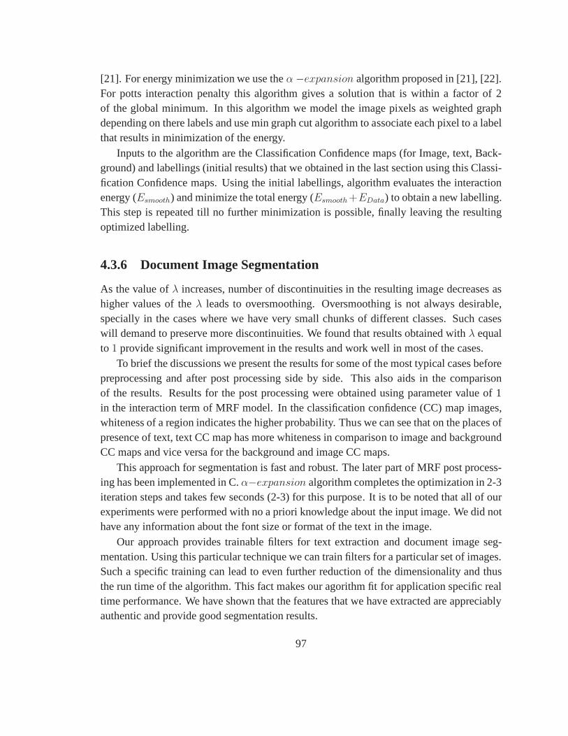
[21]. For energy minimization we use theα−expansion algorithm proposed in [21], [22].For potts interaction penalty this algorithm gives a solution that is within a factor of 2of the global minimum. In this algorithm we model the image pixels as weighted graphdepending on there labels and use min graph cut algorithm to associate each pixel to a labelthat results in minimization of the energy.
Inputs to the algorithm are the Classification Confidence maps (for Image, text, Back-ground) and labellings (initial results) that we obtained in the last section using this Classi-fication Confidence maps. Using the initial labellings, algorithm evaluates the interactionenergy (Esmooth) and minimize the total energy (Esmooth +EData) to obtain a new labelling.This step is repeated till no further minimization is possible, finally leaving the resultingoptimized labelling.
4.3.6 Document Image Segmentation
As the value ofλ increases, number of discontinuities in the resulting image decreases ashigher values of theλ leads to oversmoothing. Oversmoothing is not always desirable,specially in the cases where we have very small chunks of different classes. Such caseswill demand to preserve more discontinuities. We found thatresults obtained withλ equalto 1 provide significant improvement in the results and work wellin most of the cases.
To brief the discussions we present the results for some of the most typical cases beforepreprocessing and after post processing side by side. This also aids in the comparisonof the results. Results for the post processing were obtained using parameter value of 1in the interaction term of MRF model. In the classification confidence (CC) map images,whiteness of a region indicates the higher probability. Thus we can see that on the places ofpresence of text, text CC map has more whiteness in comparison to image and backgroundCC maps and vice versa for the background and image CC maps.
This approach for segmentation is fast and robust. The laterpart of MRF post process-ing has been implemented in C.α−expansion algorithm completes the optimization in 2-3iteration steps and takes few seconds (2-3) for this purpose. It is to be noted that all of ourexperiments were performed with no a priori knowledge aboutthe input image. We did nothave any information about the font size or format of the textin the image.
Our approach provides trainable filters for text extractionand document image seg-mentation. Using this particular technique we can train filters for a particular set of images.Such a specific training can lead to even further reduction ofthe dimensionality and thusthe run time of the algorithm. This fact makes our agorithm fitfor application specific realtime performance. We have shown that the features that we have extracted are appreciablyauthentic and provide good segmentation results.
97
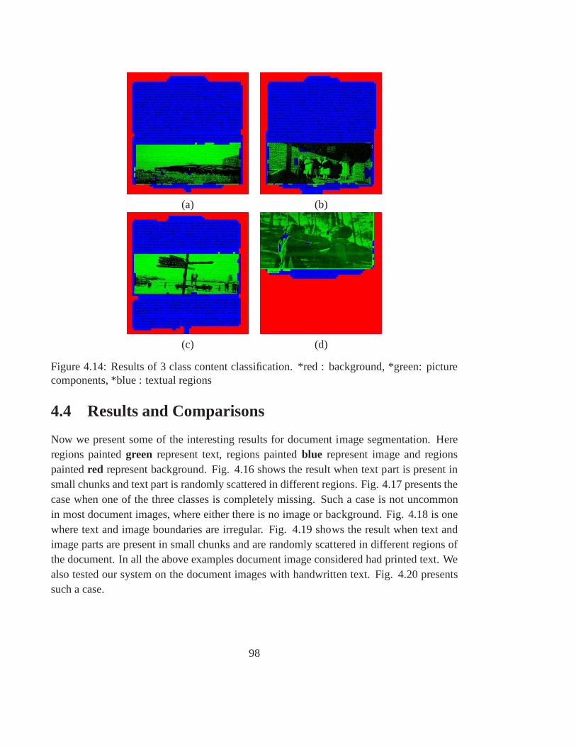
(a) (b)
(c) (d)
Figure 4.14: Results of 3 class content classification. *red: background, *green: picturecomponents, *blue : textual regions
4.4 Results and Comparisons
Now we present some of the interesting results for document image segmentation. Hereregions paintedgreen represent text, regions paintedblue represent image and regionspaintedred represent background. Fig. 4.16 shows the result when text part is present insmall chunks and text part is randomly scattered in different regions. Fig. 4.17 presents thecase when one of the three classes is completely missing. Such a case is not uncommonin most document images, where either there is no image or background. Fig. 4.18 is onewhere text and image boundaries are irregular. Fig. 4.19 shows the result when text andimage parts are present in small chunks and are randomly scattered in different regions ofthe document. In all the above examples document image considered had printed text. Wealso tested our system on the document images with handwritten text. Fig. 4.20 presentssuch a case.
98
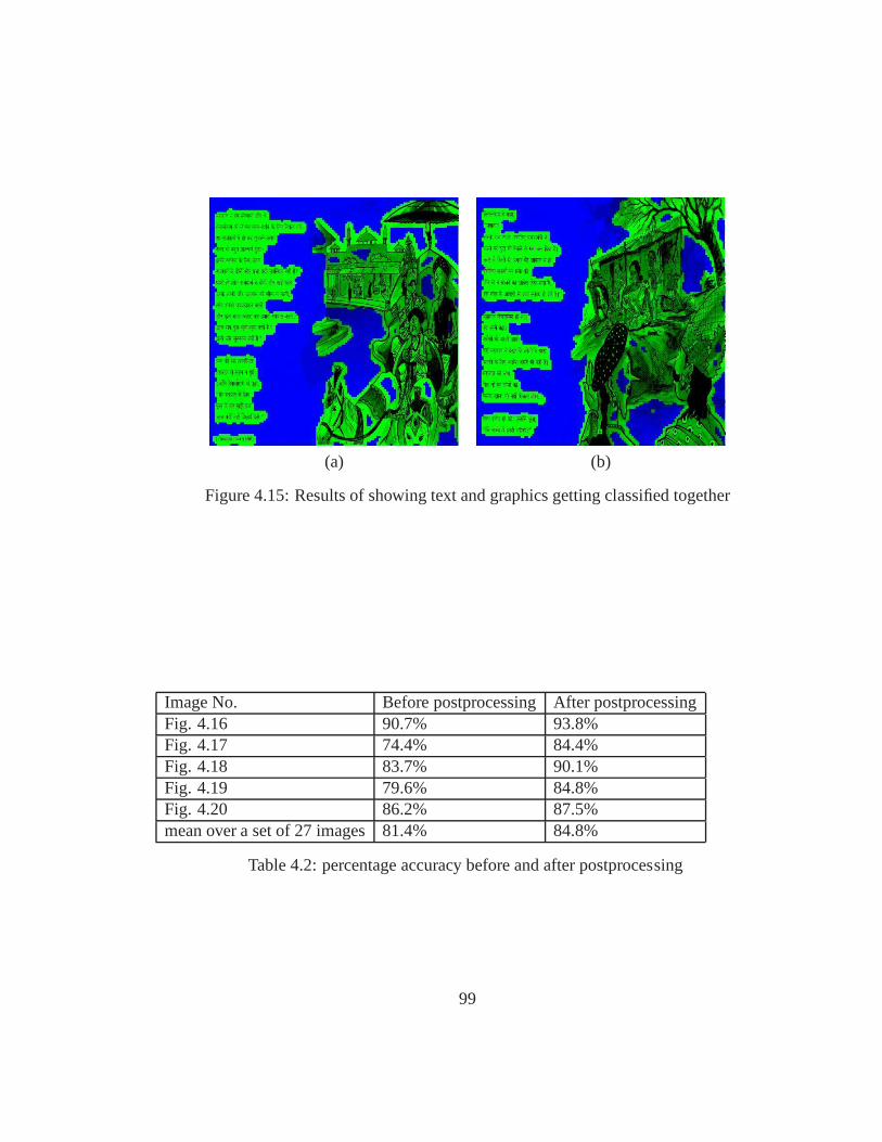
(a) (b)
Figure 4.15: Results of showing text and graphics getting classified together
Image No. Before postprocessingAfter postprocessingFig. 4.16 90.7% 93.8%Fig. 4.17 74.4% 84.4%Fig. 4.18 83.7% 90.1%Fig. 4.19 79.6% 84.8%Fig. 4.20 86.2% 87.5%mean over a set of 27 images81.4% 84.8%
Table 4.2: percentage accuracy before and after postprocessing
99
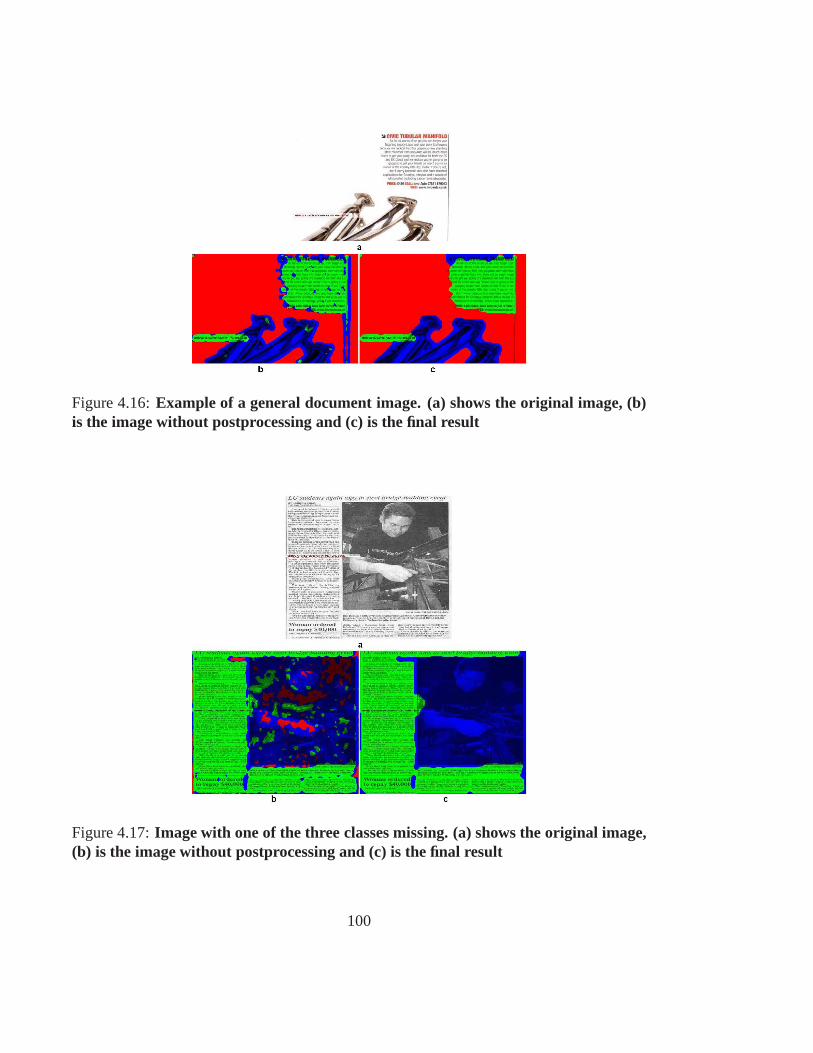
Figure 4.16:Example of a general document image. (a) shows the original image, (b)is the image without postprocessing and (c) is the final result
Figure 4.17:Image with one of the three classes missing. (a) shows the original image,(b) is the image without postprocessing and (c) is the final result
100
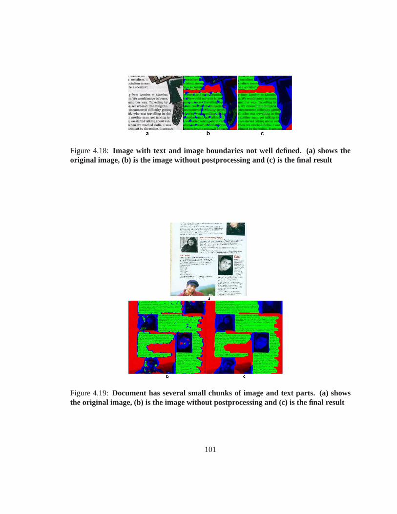
Figure 4.18: Image with text and image boundaries not well defined. (a) shows theoriginal image, (b) is the image without postprocessing and(c) is the final result
Figure 4.19:Document has several small chunks of image and text parts. (a) showsthe original image, (b) is the image without postprocessingand (c) is the final result
101

Figure 4.20:Document image with handwritten text. (a) shows the original image, (b)is the image without postprocessing and (c) is the final result
102
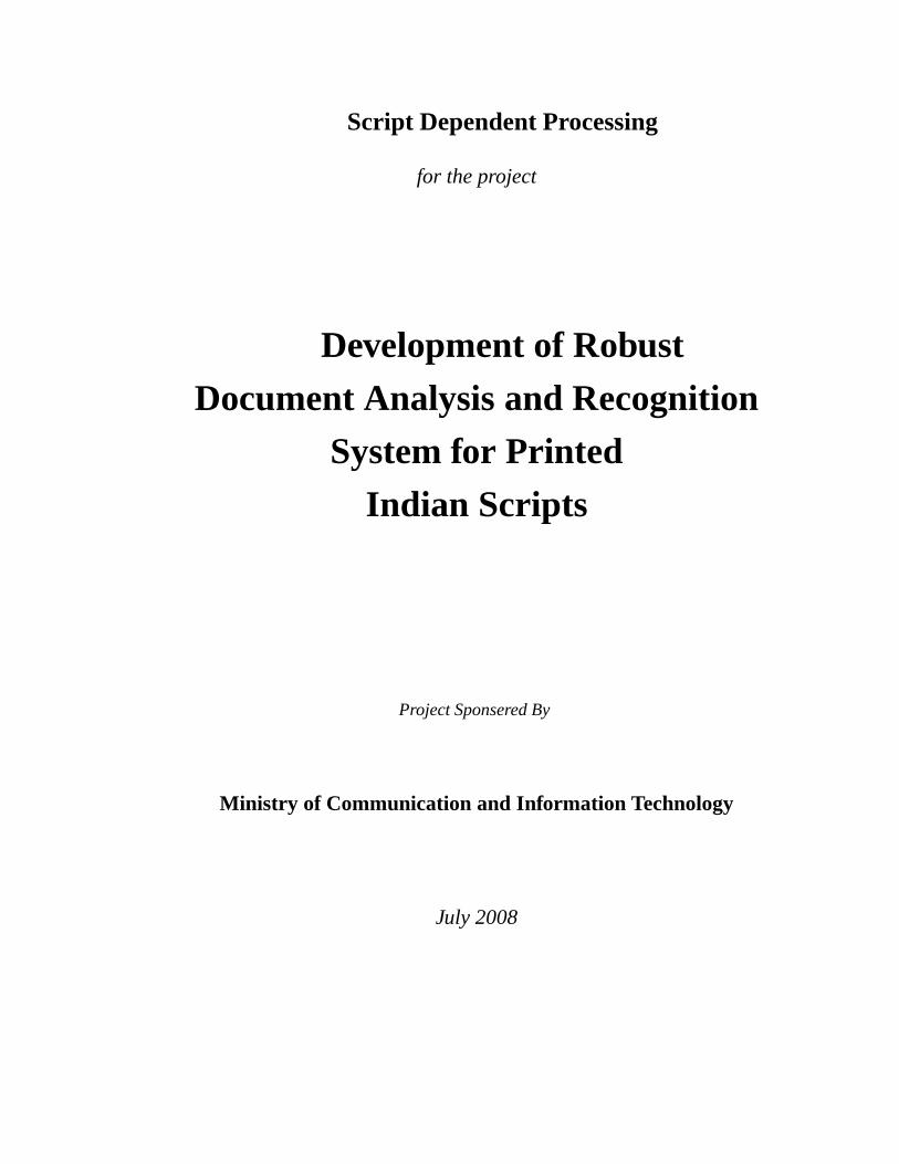
Script Dependent Processing
for the project
Development of Robust
Document Analysis and Recognition
System for Printed
Indian Scripts
Project Sponsered By
Ministry of Communication and Information Technology
July 2008

Chapter 5
Script-Dependent Processing : UnicodeGeneration
Segmentation and classification are the two primary phases of a text recognition system.The segmentation process extracts recognition units from the text. The recognition unit isusually a character. The classification process computes certain features for each isolatedcharacter and each character is classified to a class which may be the true class (correctrecognition), wrong class (substitution error), or an unknown class (rejection error). Basedon the output of the classification process, re-segmentation of selected units is attempted[23], [24] and reclassification is done. However, some classification errors still remainwhich many researchers have tried to correct using contextual knowledge [25], [26], [27,28, 29, 30].
More than one classifying feature have been employed for classification to take careof different discriminating features under varying real-life situation [31], [32]. In otherwords, the contextual knowledge is used during the classification phase also [33]. Sinha etal. [34], [35], [3] and some other researchers [36], [37] have reported various aspects ofDevanagari script recognition. An optical character recognition (OCR) for Devanagari andBangla (an Indian language script) printed script has been described by Chaudhuri and Pal[38], [39]. The emphasis is on recognizing the vowels and consonants (basic characters)which constitute 94-96% of the text. The basic characters are described in terms of ninetypes of strokes. A stroke is described in terms of its length, height and expected angle.These angles are very much font specific.
In the subsequent sections we shall discuss some useful techniques for designing high-performance trainable classifiers for the purpose of recognizing Indian-scripts’ symbols.However extraction of recognition units from text regions in a document page may posedifficulties requiring use of certain script dependent techniques. We provide the generic all
105
encompassing architecture for the script dependent processing module in the next section.
5.1 Architecture of Script Dependent OCR module
Making an OCR delivering high-performance output for Indian scripts would invariablyinvolve making use of techniques tuned to script specific characteristics. Due to the widelyvarying nature of Indian scripts, such knowledge needs to beincorporated at the line seg-mentation state itself and throughout intermediate stagesto the final output. Fig 5.1 showsthe architecture for script dependent processing for Indian Scripts. This module will re-ceive as input hypothesized line and word boundaries from script independent component.These hypotheses will be refined/modified by the script dependent processing.
The different modules in this architecture are discussed asfollows.
⋆ Line Segmentation:The presence of ascenders and descenders in some Indian scriptslike Hindi can make it difficult to demarcate the text lines using a simple cue like inter-line white space separation. A technique robust enough to deal with the merging oftext lines at the ascenders or descenders is required. Problem occurs when we get nozero horizontal profile (HP) between two lines. Expected scenario lower modifier/s ofthe above line and upper modifier/s of lower line may overlap or end row of the lowermodifier/s of the above line and the starting row of the upper modifier/s of lower linemay overlap. A sample with this type of problem is shown in Fig5.2. The two lines areproduced as a single line by the line segmentation module.
⋆ Word Segmentation: Word segmentation can be reliably done using the white spaceseparating adjacent words. However, there may be typical cases where document noisemay defy the white space assumption. Such cases need to be handled.
⋆ Symbol Extraction: Extraction of symbols from a word image is the most difficultchallenge for Indian scripts. Despite using script specificinformation the combina-torics of character conjuncts,matras, half characters, ligatures, etc. make it difficult tohave correct symbols getting extracted. Steps like removalof shiro-rekha, detection ofconjuncts, etc. are part of this module. A symbol can be a single character or a conjunctof multiple characters/matras. Touching and broken characters make the problem moredifficult.
⋆ Feature Extraction: A segmented symbol exists in the form of an image segmentcomprising a set of pixels. Good features from the pattern tobe classified are the keyto the success of any classifier system. The features should have high discriminability
106
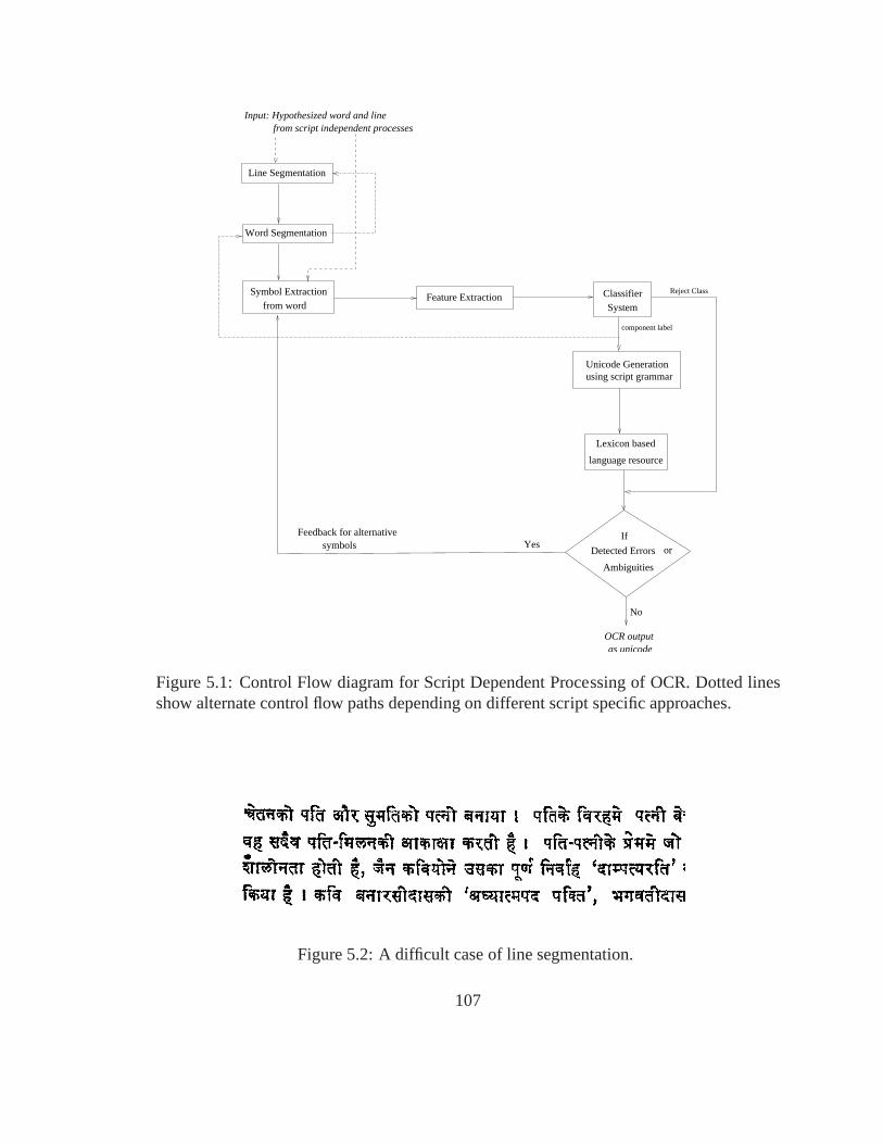
Symbol Extractionfrom word
Word Segmentation
Line Segmentation
Feature Extraction ClassifierSystem
Unicode Generationusing script grammar
Detected Errors
Ambiguities
or If
No
Yes
as unicodeOCR output
symbolsFeedback for alternative
Reject Class
component label
Lexicon based
language resource
Input: Hypothesized word and linefrom script independent processes
Figure 5.1: Control Flow diagram for Script Dependent Processing of OCR. Dotted linesshow alternate control flow paths depending on different script specific approaches.
Figure 5.2: A difficult case of line segmentation.
107
and computationally fast to extract. Furthermore, robustness to variations in differentinstances of input pattern is an essential requirement of the features. Different scriptswill make use of a different set of features tuned to an optimal OCR performance.
⋆ Classifier System:The classifier is the heart of any pattern recognition system. Theclassifier must be trainable to deliver a high output accuracy for its targeted class ofdocuments. Since the entire OCR system has to developed so asto provide its APIs, theclassifier system should be re-usable to be trained and used for similar or other scripts.
⋆ Unicode Generation using Script Grammar: For many script (eg. Malayalam) cer-tain symbols may correspond to different language characters depending on the contextSymbols occurring before and after certain symbols/characters get combined in one ofthe vowel modifiers for some languages (eg. Bangla). A rule-based system is requiredfor mapping recognized symbols to Unicode. The Unicode generation module wouldmap the component labels (the output of the classifier) to theUnicode for the symbols.The classifier output is in the form of a ranked list (with confidence) of the possiblelabels for the components. This information can be useful when applying the linguisticcontext.
⋆ Lexicon-based language resources:This module validates the Unicode stream againstthe language model of the script. It makes use of the lexicon-based information to cor-rect possible OCR errors. Such language specific constraints which are used to correctthe OCR output are called as language resources for post-OCRerror correction. Thelinguistic context can be modeled using the use of letter n-grams, lexicons and syn-tax. This module is discussed in chapter 13 where a probabilistic approach to modelingOCR input-output process has been described.
⋆ Feedback in case of ambiguities/errors:The script dependent processing architecturehas the provision of providing feedback in case of ambiguities or errors in classifica-tion. If the classifier declares the symbol to be of reject class, or the decision confidenceof the top two best classes is comparable leading to an ambiguity which cannot be re-solved even with the help of language resources, it is worthwhile to try out a differentsegmentation of the word into components. When the word segmentation module re-ceives the feedback, it produces a different possible segmentation to give components,which could be possibly recognized better with the classifier.
108

Chapter 6
Telugu OCR System: Classifier Designand Implementation
The Telugu OCR system recognizes connected components thatare assembled into legalcharacters and stored in Unicode format. The exact number ofconnected components forrecognition by the classifier is font-dependent but varies between 350 and 450. This reportdescribes the strategies evolved by our team to handle such alarge number of classes andother technical details.
The primary strategy in handling the large number of classesis to cluster the individualcharacters into groups and then classify the characters within each group. We experimentedprimarily with two ways of clustering: based on the languagestructure, and on image-levelfeatures.
6.1 Language structure based clustering
The characters in Telugu language fall naturally into threebroad categories:vowels, conso-nants and their vowel-modified variantsandconsonant-modifiers. A consonant and all itsvowel-modified variants is called aguninthamin Telugu and defines a natural cluster. Asthere are 35 consonants, there are 35 gunintham clusters. Each vowel, on the other hand,has a distinct shape resulting in another 11 classes. However, two of the vowels are similarin shape to the consonantpa, and are added to thepa-guninthamcluster. Thus, the totalnumber of clusters is 44 with each of the 35 guninatham clusters containing roughly 11characters. Figure 6.1 shows the members of theka gunintham.
Some of the clusters contain less than 11 characters becausea few vowel modifiers arenot connected to the base character and therefore do not alter the connected component
109
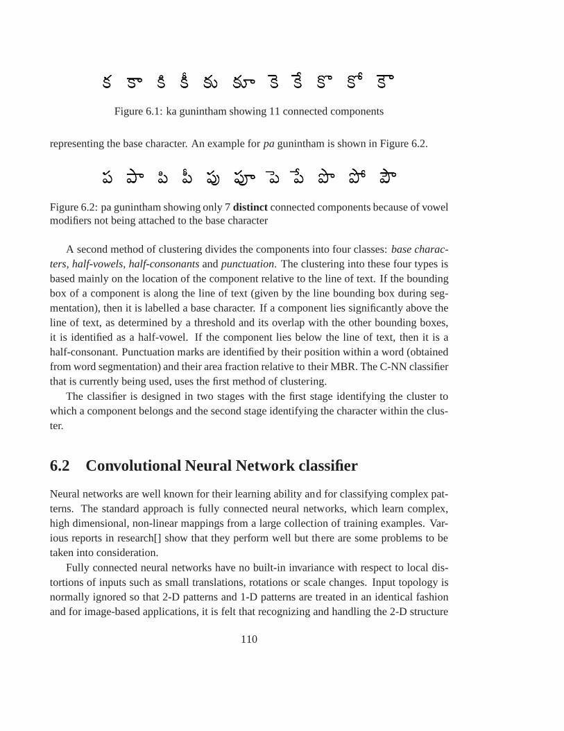
Figure 6.1: ka gunintham showing 11 connected components
representing the base character. An example forpagunintham is shown in Figure 6.2.
Figure 6.2: pa gunintham showing only 7distinct connected components because of vowelmodifiers not being attached to the base character
A second method of clustering divides the components into four classes:base charac-ters, half-vowels, half-consonantsandpunctuation. The clustering into these four types isbased mainly on the location of the component relative to theline of text. If the boundingbox of a component is along the line of text (given by the line bounding box during seg-mentation), then it is labelled a base character. If a component lies significantly above theline of text, as determined by a threshold and its overlap with the other bounding boxes,it is identified as a half-vowel. If the component lies below the line of text, then it is ahalf-consonant. Punctuation marks are identified by their position within a word (obtainedfrom word segmentation) and their area fraction relative totheir MBR. The C-NN classifierthat is currently being used, uses the first method of clustering.
The classifier is designed in two stages with the first stage identifying the cluster towhich a component belongs and the second stage identifying the character within the clus-ter.
6.2 Convolutional Neural Network classifier
Neural networks are well known for their learning ability and for classifying complex pat-terns. The standard approach is fully connected neural networks, which learn complex,high dimensional, non-linear mappings from a large collection of training examples. Var-ious reports in research[] show that they perform well but there are some problems to betaken into consideration.
Fully connected neural networks have no built-in invariance with respect to local dis-tortions of inputs such as small translations, rotations orscale changes. Input topology isnormally ignored so that 2-D patterns and 1-D patterns are treated in an identical fashionand for image-based applications, it is felt that recognizing and handling the 2-D structure
110
may produce better results. Adjacent pixels in an image are highly correlated and havebeen greatly exploited in convolution based spatial image processing operations to extractlocal features such as edges. For images with even a few hundred rows and columns, afully connected network requires training an extremely large number of weights which, inturn, may require prohibitively large training sets and result in very long training times.
6.2.1 Convolutional neural networks
Convolutional networks use three ideasviz. local receptive fields, shared weights and sub-sampling to overcome the problems stated above with fully connected networks[?]. Theuse of local receptive fields mimics convolutional masks andsimultaneously handle 2Dtopography of images while retaining and exploiting local correlations. As the local fieldsare replicated across the entire layer, the number of weights to learn is reduced to the sizeof the local receptive field. Shared weights simulate the effect of convolution while spatialsub-sampling allows small local distortions to be handled in an effective manner.
These ideas are translated into two new architectural features:convolutoinal layerandthesub-sampling layer. In a convolutional layer each unit takes the input from a setof unitslocated in small neighbourhood of pre-fixed size defined by a convolution kernel from theprevious layer. The idea of connecting units to local receptive fields on the input goes backto Perceptron of late 60’s[]. Each unit has kernel size inputs, and for each input unit thereexists a set of trainable coefficients of kernel size plus a trainable bias.
Distortion or shifts of the input can cause the position of salient features to vary. Inaddition elementary feature detectors that are useful on one part of the image are likely tobe useful across the entire image. This knowledge can be applied by forcing a set of units,whose receptive fields are located at different places on theimage, to have identical weightvectors in a single place.
The set of outputs resulting from a single unit are called as feature map. A completeconvolutional layer is composed of several feature maps which can be extracted at eachlocation. The receptive fields of contiguous units in a feature map are centered on corre-sponding contiguous units in the previous layer. Thereforereceptive fields of horizontallycontiguous units overlap.
An interesting property of convolutional layer is that, if the input image is shifted,the feature map output will be shifted by the same amount, butwill be left unchangedotherwise. This property is the basis of the robustness of convolutional networks to shiftsand distortion of the input.
Once a feature has been detected, its exact location becomesless important. Only itsappropriate position relative to other feature is relevant. Not only is the precise position
111
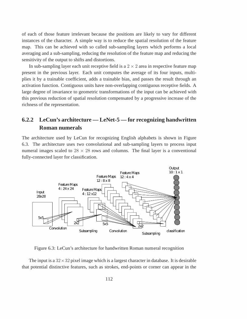
of each of those feature irrelevant because the positions are likely to vary for differentinstances of the character. A simple way is to reduce the spatial resolution of the featuremap. This can be achieved with so called sub-sampling layerswhich performs a localaveraging and a sub-sampling, reducing the resolution of the feature map and reducing thesensitivity of the output to shifts and distortions.
In sub-sampling layer each unit receptive field is a2× 2 area in respective feature mappresent in the previous layer. Each unit computes the average of its four inputs, multi-plies it by a trainable coefficient, adds a trainable bias, and passes the result through anactivation function. Contiguous units have non-overlapping contiguous receptive fields. Alarge degree of invariance to geometric transformations ofthe input can be achieved withthis previous reduction of spatial resolution compensatedby a progressive increase of therichness of the representation.
6.2.2 LeCun’s architecture — LeNet-5 — for recognizing handwrittenRoman numerals
The architecture used by LeCun for recognizing English alphabets is shown in Figure6.3. The architecture uses two convolutional and sub-sampling layers to process inputnumeral images scaled to28 × 28 rows and columns. The final layer is a conventionalfully-connected layer for classification.
Figure 6.3: LeCun’s architecture for handwritten Roman numeral recognition
The input is a32×32 pixel image which is a largest character in database. It is desirablethat potential distinctive features, such as strokes, end-points or corner can appear in the
112
center of the receptive field of the highest level feature detectors.
Layer 1 is a convolutional layer with 6 feature maps each unitin feature map is con-nected to be a5 × 5 neighborhood in the input. Each unit in a feature map has 25 inputsconnected to a5 × 5 area input which is its receptive field. As each unit has 25 inputs,therefore 25 trainable coefficients plus a trainable bias. The resultant feature map size is28× 28. This layer contains 156 trainable parameters and 122,304 connections.
All the units in a feature map share the same set of 25 weights and the same bias, sothey detected the same feature at all possible locations in the input. The other feature mapsin the layer use different sets of weights and bias, there by extracting different types of localfeatures. In LeNet-5 at each location six different features are extracted form six units inidentical location in the six feature maps.
Layer 2 is a Sub-sampling layer with four feature maps of size14× 14. The receptivefields of each unit are non-overlapping, therefore feature map of layer 2 have half the num-ber of rows and columns of feature map of layer 1. This layer has 12 trainable parametersand 5,810 connections.
Layer 3 is a convolutional layer with 16 feature maps. Each unit in each feature map isconnected to several5×5 neighborhoods at identical location of a subset of layer 2 featuremaps to extract different features. This layer has 1,516 trainable parameters and 1,56,000connections.
Layer 4 is a Sub-sampling layer with 16 feature maps of size5 × 5 similar to layer 2,has 34 trainable parameters , and 2,000 connections.
Layer 5 is a convolutional layer with 120 feature maps. As thesize of layer 4 featuremap is also5 × 5, the size of layer 5 feature map is1 × 1. This layer contains 48,120connections.
Layer 6 contains 84 units and is a fully connected to layer 5. This layer has 10,164parameters.
As C-NN architecture is usingweight sharingconcept the architecture shown in Figure6.3 contains 345,308 connections, but only 60,000 trainable free parameters.
6.3 Multi-class C-NN Classifier for Telugu Components
We conducted a series of experiments to evaluate the effectiveness of C-NN in classifyingTelugu components. The C-NNs are used to classify a given test character into one ofthe 44 classes described in Section 6.1. Initially, we varied the number of layers and thenumber of feature maps and discovered that the number of clusters that can be reliablyrecognized is about 10. Later we built a hybrid architecturecombining 5 C-NNs with a
113

fully connected layer to design a complete classifier for the44 classes. In this section, wereport our experimental results in detail.
6.3.1 Architecture – 1
We have started our multi-class classifier experiments withthe simple architecture shownin Figure 6.4 which performed well for the binary classification. The C-NN includes asingle convolution layer that has four neuron units resulting in four feature maps, followedby two fully connected layers. This architecture uses a5× 5 kernel which is the trainablecoefficient matrix for convolution operation. The output layer has five neuron units in theoutput layer to recognize five classes. In our experiments wegradually increase the numberof classes to be handled by the classifier and observe the performance of classifier then wemodify the architecture to improve its performance by increasing number of hidden unitsused in convolution layer.
Figure 6.4: C-NN Architecture-1 used for Telugu OCR
Results and Observations
This five-class classifier is trained with 160 sample images for each class. Test set is of 200images for each class which includes training set 160 samples in it, apart from training set
114
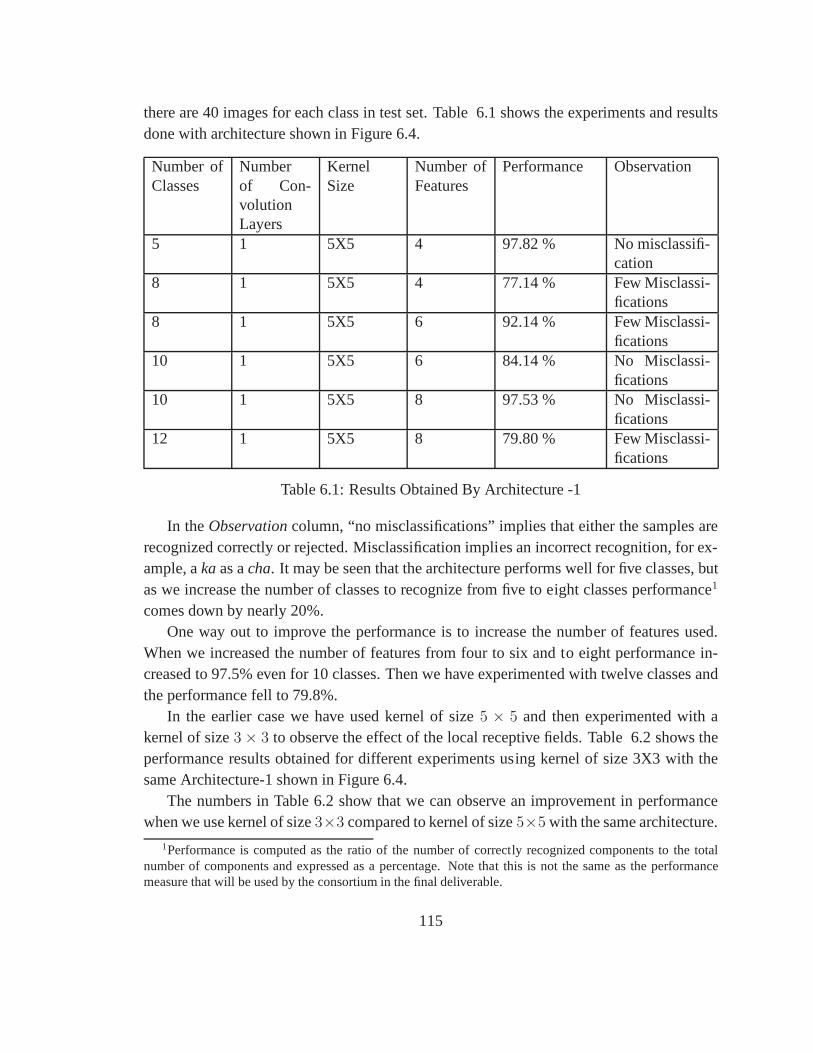
there are 40 images for each class in test set. Table 6.1 showsthe experiments and resultsdone with architecture shown in Figure 6.4.
Number ofClasses
Numberof Con-volutionLayers
KernelSize
Number ofFeatures
Performance Observation
5 1 5X5 4 97.82 % No misclassifi-cation
8 1 5X5 4 77.14 % Few Misclassi-fications
8 1 5X5 6 92.14 % Few Misclassi-fications
10 1 5X5 6 84.14 % No Misclassi-fications
10 1 5X5 8 97.53 % No Misclassi-fications
12 1 5X5 8 79.80 % Few Misclassi-fications
Table 6.1: Results Obtained By Architecture -1
In theObservationcolumn, “no misclassifications” implies that either the samples arerecognized correctly or rejected. Misclassification implies an incorrect recognition, for ex-ample, akaas acha. It may be seen that the architecture performs well for five classes, butas we increase the number of classes to recognize from five to eight classes performance1
comes down by nearly 20%.One way out to improve the performance is to increase the number of features used.
When we increased the number of features from four to six and to eight performance in-creased to 97.5% even for 10 classes. Then we have experimented with twelve classes andthe performance fell to 79.8%.
In the earlier case we have used kernel of size5 × 5 and then experimented with akernel of size3× 3 to observe the effect of the local receptive fields. Table 6.2shows theperformance results obtained for different experiments using kernel of size 3X3 with thesame Architecture-1 shown in Figure 6.4.
The numbers in Table 6.2 show that we can observe an improvement in performancewhen we use kernel of size3×3 compared to kernel of size5×5 with the same architecture.
1Performance is computed as the ratio of the number of correctly recognized components to the totalnumber of components and expressed as a percentage. Note that this is not the same as the performancemeasure that will be used by the consortium in the final deliverable.
115
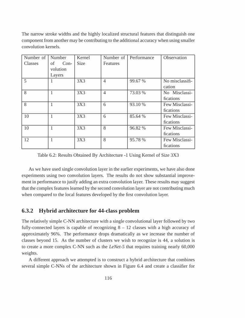
The narrow stroke widths and the highly localized structural features that distinguish onecomponent from another may be contributing to the additional accuracy when using smallerconvolution kernels.
Number ofClasses
Numberof Con-volutionLayers
KernelSize
Number ofFeatures
Performance Observation
5 1 3X3 4 99.67 % No misclassifi-cation
8 1 3X3 4 73.03 % No Misclassi-fications
8 1 3X3 6 93.10 % Few Misclassi-fications
10 1 3X3 6 85.64 % Few Misclassi-fications
10 1 3X3 8 96.82 % Few Misclassi-fications
12 1 3X3 8 95.78 % Few Misclassi-fications
Table 6.2: Results Obtained By Architecture -1 Using Kernelof Size 3X3
As we have used single convolution layer in the earlier experiments, we have also doneexperiments using two convolution layers. The results do not show substantial improve-ment in performance to jusify adding an extra convolution layer. These results may suggestthat the complex features learned by the second convolutionlayer are not contributing muchwhen compared to the local features developed by the first convolution layer.
6.3.2 Hybrid architecture for 44-class problem
The relatively simple C-NN architecture with a single convolutional layer followed by twofully-connected layers is capable of recognizing 8 – 12 classes with a high accuracy ofapproximately 96%. The performance drops dramatically as we increase the number ofclasses beyond 15. As the number of clusters we wish to recognize is 44, a solution isto create a more complex C-NN such as theLeNet-5that requires training nearly 60,000weights.
A different approach we attempted is to construct a hybrid architecture that combinesseveral simple C-NNs of the architecture shown in Figure 6.4and create a classifier for
116
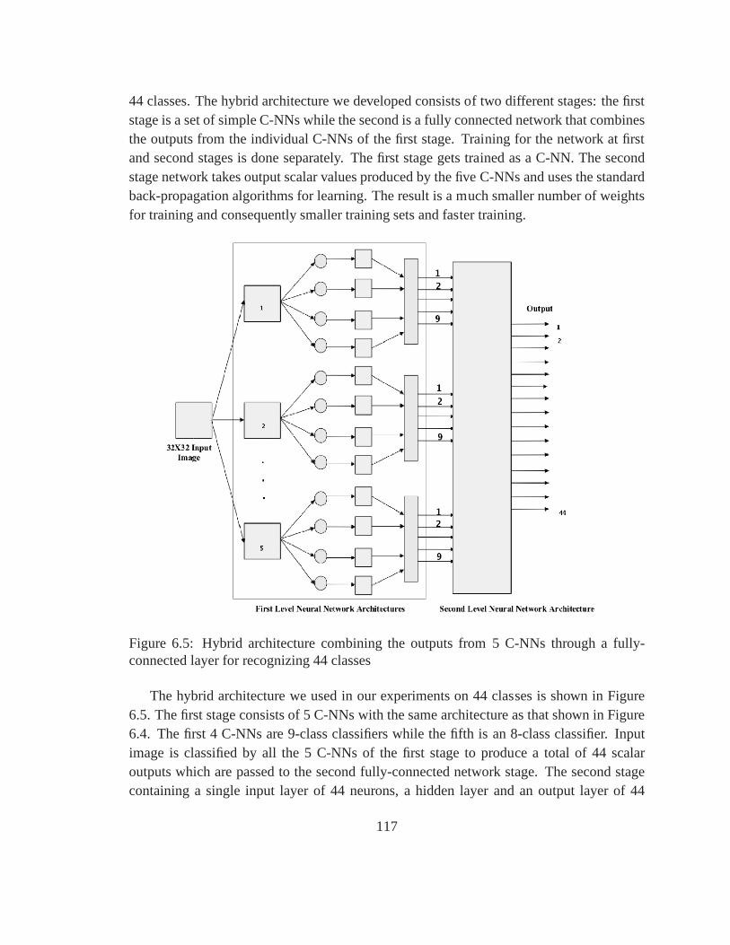
44 classes. The hybrid architecture we developed consists of two different stages: the firststage is a set of simple C-NNs while the second is a fully connected network that combinesthe outputs from the individual C-NNs of the first stage. Training for the network at firstand second stages is done separately. The first stage gets trained as a C-NN. The secondstage network takes output scalar values produced by the fiveC-NNs and uses the standardback-propagation algorithms for learning. The result is a much smaller number of weightsfor training and consequently smaller training sets and faster training.
Figure 6.5: Hybrid architecture combining the outputs from5 C-NNs through a fully-connected layer for recognizing 44 classes
The hybrid architecture we used in our experiments on 44 classes is shown in Figure6.5. The first stage consists of 5 C-NNs with the same architecture as that shown in Figure6.4. The first 4 C-NNs are 9-class classifiers while the fifth isan 8-class classifier. Inputimage is classified by all the 5 C-NNs of the first stage to produce a total of 44 scalaroutputs which are passed to the second fully-connected network stage. The second stagecontaining a single input layer of 44 neurons, a hidden layerand an output layer of 44
117
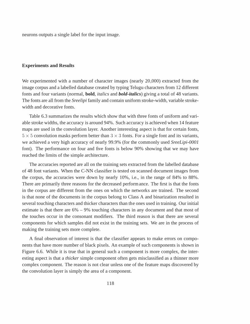
neurons outputs a single label for the input image.
Experiments and Results
We experimented with a number of character images (nearly 20,000) extracted from theimage corpus and a labelled database created by typing Telugu characters from 12 differentfonts and four variants (normal,bold, italics andbold-italics) giving a total of 48 variants.The fonts are all from theSreelipifamily and contain uniform stroke-width, variable stroke-width and decorative fonts.
Table 6.3 summarizes the results which show that with three fonts of uniform and vari-able stroke widths, the accuracy is around 94%. Such accuracy is achieved when 14 featuremaps are used in the convolution layer. Another interestingaspect is that for certain fonts,5× 5 convolution masks perform better than3× 3 fonts. For a single font and its variants,we achieved a very high accuracy of nearly 99.9% (for the commonly usedSreeLipi-0001font). The performance on four and five fonts is below 90% showing that we may havereached the limits of the simple architecture.
The accuracies reported are all on the training sets extracted from the labelled databaseof 48 font variants. When the C-NN classifier is tested on scanned document images fromthe corpus, the accuracies were down by nearly 10%, i.e., in the range of 84% to 88%.There are primarily three reasons for the decreased performance. The first is that the fontsin the corpus are different from the ones on which the networks are trained. The secondis that none of the documents in the corpus belong to Class A and binarization resulted inseveral touching characters and thicker characters than the ones used in training. Our initialestimate is that there are 6% – 9% touching characters in any document and that most ofthe touches occur in the consonant modifiers. The third reason is that there are severalcomponents for which samples did not exist in the training sets. We are in the process ofmaking the training sets more complete.
A final observation of interest is that the classifier appearsto make errors on compo-nents that have more number of black pixels. An example of such components is shown inFigure 6.6. While it is true that in general such a component is more complex, the inter-esting aspect is that athickersimple component often gets misclassified as a thinner morecomplex component. The reason is not clear unless one of the feature maps discovered bythe convolution layer is simply the area of a component.
118
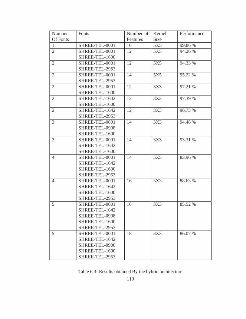
NumberOf Fonts
Fonts Number ofFeatures
KernelSize
Performance
1 SHREE-TEL-0001 10 5X5 99.86 %2 SHREE-TEL-0001
SHREE-TEL-160012 5X5 94.26 %
2 SHREE-TEL-0001SHREE-TEL-2953
12 5X5 94.33 %
2 SHREE-TEL-0001SHREE-TEL-2953
14 5X5 95.22 %
2 SHREE-TEL-0001SHREE-TEL-1600
12 3X3 97.21 %
2 SHREE-TEL-1642SHREE-TEL-1600
12 3X3 97.39 %
2 SHREE-TEL-1642SHREE-TEL-2953
12 3X3 96.73 %
3 SHREE-TEL-0001SHREE-TEL-0908SHREE-TEL-1600
14 3X3 94.48 %
3 SHREE-TEL-0001SHREE-TEL-1642SHREE-TEL-1600
14 3X3 93.31 %
4 SHREE-TEL-0001SHREE-TEL-1642SHREE-TEL-1600SHREE-TEL-2953
14 5X5 83.96 %
4 SHREE-TEL-0001SHREE-TEL-1642SHREE-TEL-1600SHREE-TEL-2953
16 3X3 88.63 %
5 SHREE-TEL-0001SHREE-TEL-1642SHREE-TEL-0908SHREE-TEL-1600SHREE-TEL-2953
16 3X3 85.52 %
5 SHREE-TEL-0001SHREE-TEL-1642SHREE-TEL-0908SHREE-TEL-1600SHREE-TEL-2953
18 3X3 86.07 %
Table 6.3: Results obtained By the hybrid architecture
119
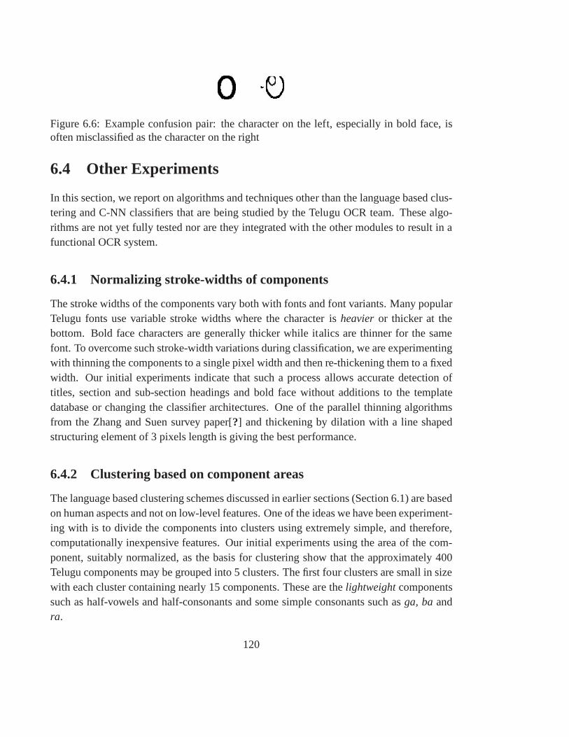
Figure 6.6: Example confusion pair: the character on the left, especially in bold face, isoften misclassified as the character on the right
6.4 Other Experiments
In this section, we report on algorithms and techniques other than the language based clus-tering and C-NN classifiers that are being studied by the Telugu OCR team. These algo-rithms are not yet fully tested nor are they integrated with the other modules to result in afunctional OCR system.
6.4.1 Normalizing stroke-widths of components
The stroke widths of the components vary both with fonts and font variants. Many popularTelugu fonts use variable stroke widths where the characteris heavieror thicker at thebottom. Bold face characters are generally thicker while italics are thinner for the samefont. To overcome such stroke-width variations during classification, we are experimentingwith thinning the components to a single pixel width and thenre-thickening them to a fixedwidth. Our initial experiments indicate that such a processallows accurate detection oftitles, section and sub-section headings and bold face without additions to the templatedatabase or changing the classifier architectures. One of the parallel thinning algorithmsfrom the Zhang and Suen survey paper[?] and thickening by dilation with a line shapedstructuring element of 3 pixels length is giving the best performance.
6.4.2 Clustering based on component areas
The language based clustering schemes discussed in earliersections (Section 6.1) are basedon human aspects and not on low-level features. One of the ideas we have been experiment-ing with is to divide the components into clusters using extremely simple, and therefore,computationally inexpensive features. Our initial experiments using the area of the com-ponent, suitably normalized, as the basis for clustering show that the approximately 400Telugu components may be grouped into 5 clusters. The first four clusters are small in sizewith each cluster containing nearly 15 components. These are thelightweightcomponentssuch as half-vowels and half-consonants and some simple consonants such asga, baandra.
120
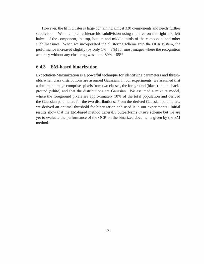
However, the fifth cluster is large containing almost 320 components and needs furthersubdivision. We attempted a hierarchic subdivision using the area on the right and lefthalves of the component, the top, bottom and middle thirds ofthe component and othersuch measures. When we incorporated the clustering scheme into the OCR system, theperformance increased slightly (by only 1% – 3%) for most images where the recognitionaccuracy without any clustering was about 80% – 85%.
6.4.3 EM-based binarization
Expectation-Maximization is a powerful technique for identifying parameters and thresh-olds when class distributions are assumed Gaussian. In our experiments, we assumed thata document image comprises pixels from two classes, the foreground (black) and the back-ground (white) and that the distributions are Gaussian. We assumed a mixture model,where the foreground pixels are approximately 10% of the total population and derivedthe Gaussian parameters for the two distributions. From thederived Gaussian parameters,we derived an optimal threshold for binarization and used itin our experiments. Initialresults show that the EM-based method generally outperforms Otsu’s scheme but we areyet to evaluate the performance of the OCR on the binarized documents given by the EMmethod.
121

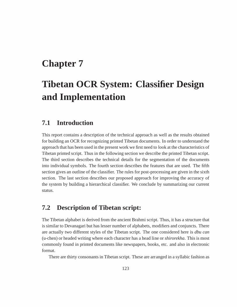
Chapter 7
Tibetan OCR System: Classifier Designand Implementation
7.1 Introduction
This report contains a description of the technical approach as well as the results obtainedfor building an OCR for recognizing printed Tibetan documents. In order to understand theapproach that has been used in the present work we first need tolook at the characteristics ofTibetan printed script. Thus in the following section we describe the printed Tibetan script.The third section describes the technical details for the segmentation of the documentsinto individual symbols. The fourth section describes the features that are used. The fifthsection gives an outline of the classifier. The rules for post-processing are given in the sixthsection. The last section describes our proposed approach for improving the accuracy ofthe system by building a hierarchical classifier. We conclude by summarizing our currentstatus.
7.2 Description of Tibetan script:
The Tibetan alphabet is derived from the ancient Brahmi script. Thus, it has a structure thatis similar to Devanagari but has lesser number of alphabets,modifiers and conjuncts. Thereare actually two different styles of the Tibetan script. Theone considered here isdbu can(u-chen) or headed writing where each character has a head line orshirorekha. This is mostcommonly found in printed documents like newspapers, books, etc. and also in electronicformat.
There are thirty consonants in Tibetan script. These are arranged in a syllabic fashion as
123
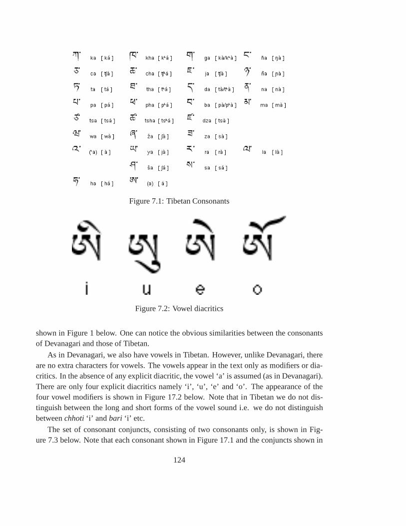
Figure 7.1: Tibetan Consonants
Figure 7.2: Vowel diacritics
shown in Figure 1 below. One can notice the obvious similarities between the consonantsof Devanagari and those of Tibetan.
As in Devanagari, we also have vowels in Tibetan. However, unlike Devanagari, thereare no extra characters for vowels. The vowels appear in the text only as modifiers or dia-critics. In the absence of any explicit diacritic, the vowel‘a’ is assumed (as in Devanagari).There are only four explicit diacritics namely ‘i’, ‘u’, ‘e’and ‘o’. The appearance of thefour vowel modifiers is shown in Figure 17.2 below. Note that in Tibetan we do not dis-tinguish between the long and short forms of the vowel sound i.e. we do not distinguishbetweenchhoti‘i’ and bari ‘i’ etc.
The set of consonant conjuncts, consisting of two consonants only, is shown in Fig-ure 7.3 below. Note that each consonant shown in Figure 17.1 and the conjuncts shown in
124
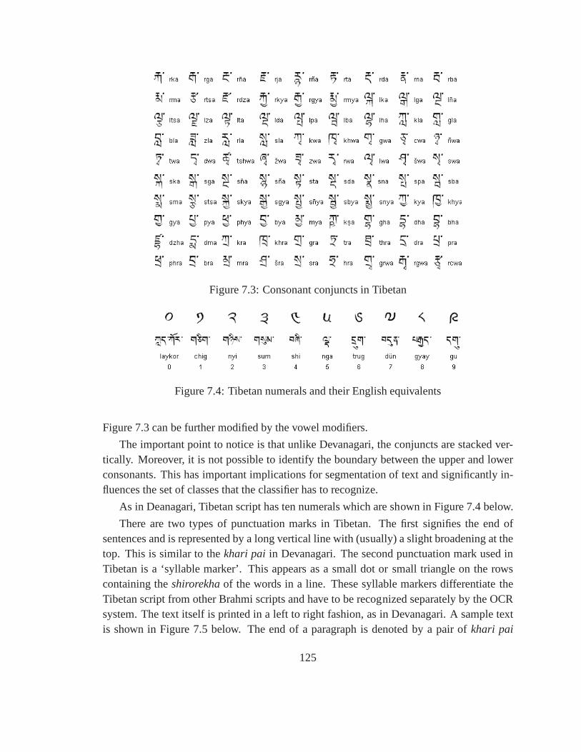
Figure 7.3: Consonant conjuncts in Tibetan
Figure 7.4: Tibetan numerals and their English equivalents
Figure 7.3 can be further modified by the vowel modifiers.
The important point to notice is that unlike Devanagari, theconjuncts are stacked ver-tically. Moreover, it is not possible to identify the boundary between the upper and lowerconsonants. This has important implications for segmentation of text and significantly in-fluences the set of classes that the classifier has to recognize.
As in Deanagari, Tibetan script has ten numerals which are shown in Figure 7.4 below.
There are two types of punctuation marks in Tibetan. The firstsignifies the end ofsentences and is represented by a long vertical line with (usually) a slight broadening at thetop. This is similar to thekhari pai in Devanagari. The second punctuation mark used inTibetan is a ‘syllable marker’. This appears as a small dot orsmall triangle on the rowscontaining theshirorekhaof the words in a line. These syllable markers differentiatetheTibetan script from other Brahmi scripts and have to be recognized separately by the OCRsystem. The text itself is printed in a left to right fashion,as in Devanagari. A sample textis shown in Figure 7.5 below. The end of a paragraph is denotedby a pair ofkhari pai
125
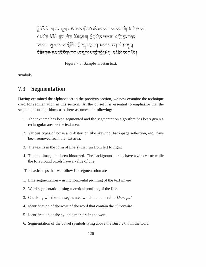
Figure 7.5: Sample Tibetan text.
symbols.
7.3 Segmentation
Having examined the alphabet set in the previous section, wenow examine the techniqueused for segmentation in this section. At the outset it is essential to emphasize that thesegmentation algorithms used here assumes the following:
1. The text area has been segmented and the segmentation algorithm has been given arectangular area as the text area.
2. Various types of noise and distortion like skewing, back-page reflection, etc. havebeen removed from the text area.
3. The text is in the form of line(s) that run from left to right.
4. The text image has been binarized. The background pixels have a zero value whilethe foreground pixels have a value of one.
The basic steps that we follow for segmentation are
1. Line segmentation – using horizontal profiling of the textimage
2. Word segmentation using a vertical profiling of the line
3. Checking whether the segmented word is a numeral orkhari pai
4. Identification of the rows of the word that contain theshirorekha
5. Identification of the syllable markers in the word
6. Segmentation of the vowel symbols lying above theshirorekhain the word
126
7. Segmentation of the symbols lying below theshirorekha
At this stage it is pertinent to point out that since the Tibetan script and grammar arestrongly influenced by the Brahmi script and Sanskrit grammar, so there is extensive usageof sandhiandsamas. Thus, quite often we find that an entire sentence constitutes of asingle word. This is true, for example, with the first word of the second line and thesecond, third and fourth words of the third line in the sampleshown in Figure 5. In thefollowing we describe each of the above steps briefly and discuss some of the issues thatwere encountered while performing the above steps and how these issues were resolved.
7.3.1 Line segmentation
This is an easy step, provided there is no skew in the text image. Simple horizontal profilingof the text image and location of zeros in the horizontal profile is adequate for segmentingthe lines. The line segmentation algorithm accepts an inputin the form of a binarized .tiffimage. The ‘libtiff’ library is used to read the image file andextract the size information aswell as the pixel values. For output, the line segmentation technique produces a linked listwith the coordinates of the bounding rectangles of the lines.
Two issues were faced with this method.
a) For some fonts there is a slight separation between the vowel modifier and the restof the character. Thus, we can get a separate line with only the vowel modifiers in it.We resolved this issue at the post-processing stage while reconstructing the originalcharacters and assigning Unicode values to them. Essentially, when we found a lineconsisting of upper vowel modifiers only, then we consideredthat line together withthe line below it, for the reconstruction purpose.
b) The assumption of perfect skew removal is an idealization. In practice there may be asmall residual skew. Thus, experiments were performed to judge the tolerance of thealgorithm to skew. It was found that for well separated lines(category A documents)the algorithm can tolerate up to 50 of skew while for dense text lines (category Bdocuments) the tolerance is for up to 20.
7.3.2 Word segmentation
The word segmentation module gets its input from the line segmentation module. Thewords are identified using vertical profiling of the line. A histogram is created of the runlengths of the white spaces (i.e. zero black pixels). This histogram shows a sharp peak
127
for small run lengths and a broader peak for large run lengths. The first corresponds tospaces between individual characters and the latter corresponds to spaces between words/ sentences. The first peak is easily identifiable and a threshold is obtained that is greaterthan the first peak. Whenever the run length of white spaces isgreater than this thresholdthen it signifies the end of a word thus leading to word segmentation. The output of thismodule is a linked list containing the coordinates of the bounding rectangle of the words.
The major issue with word segmentation is that numerals andkhari pai are also seg-mented as words. While this is not an error, it needs to be handled separately else thecharacter segmentation module will try to segment these characters, leading to errors. Theresolution of this issue is described in step 3 below.
7.3.3 Checking for numerals and khari pai
The horizontal extent of each object, generated by the word segmentation module, is mea-sured. If the horizontal extent is of the order of an individual character then the object ispassed to a small classifier that has been built to identify numerals andkhari pai. In casethe object matches with any of these eleven objects then the object is not segmented furtheri.e. it is not sent to step 4 below. In case the object does not match with any of these elevenobjects then it is sent to the next module which segments eachword into individual objectsthat have to be recognized.
7.3.4 Identification of the rows of the word that contain the shirorekha
This step is required for further segmentation of the words into individual characters and forfinding the syllable markers. The rows containing theshirorekhacan be identified from thehorizontal profile of each word. While it is true that we couldhave identified theshirorekhafrom the horizontal profile of the line, we prefer to repeat the exercise at the level of a wordbecause we have found that for some documents (of C and D category) the shirorekhafluctuates by a few pixels across words. The rows of the word that contain theshirorekhacan be identified by horizontal profiling. As in Devanagari, the number of pixels will bethe highest in these rows. Thus, the peak in the horizontal profile of a word is found. Allrows, connected to the row containing the peak value and having a pixel value more than75% of the peak value are considered to be a part of theshirorekha. This method has beentested on a large number of fonts and works well in each case.
128
7.3.5 Identification of the syllable markers in the word
As mentioned earlier, the syllable markers are small, identifiable objects that are present inthe rows containing theshirorekha. The syllable markers are separated from theshirorekhaby small white spaces in the horizontal direction. Thus, a vertical profile of the word isobtained. All objects separated by pairs of white spaces areexamined. If the vertical andhorizontal extent of any of these objects is of the order of the number of rows containingtheshirorekhaand the object lies in the same set of rows as theshirorekhathen the objectis identified as a syllable marker. The features mentioned above are sufficient for the iden-tification of syllable markers. The coordinates of the bounding rectangles of the syllablemarkers are put in a linked list which is the output of this module.
The only major issue that was identified with the above technique was that, for somefonts and some characters, the columns containing the lowermodifier ‘u’ overlaps with thecolumns containing the syllable marker. Thus, vertical profiling does not yield a zero valuefor these cases and the corresponding syllable marker is missed. This is handled in step 7described below.
7.3.6 Segmentation of the vowel symbols lying above the shirorekhain the word
Once the rows containing theshirorekhais identified in step 4 above, the segmentation ofvowel modifiers lying above theshirorekhacan be easily achieved. This is done by obtain-ing a vertical profile of the rows lying above theshirorekha. Only three symbols can comeabove theshirorekha. These are the vowel modifiers for ‘i’, ‘e’ and ‘o’. Even for densetext we did not find a single instance where two vowel modifiersoverlapped. Thus, the ver-tical profiling accurately identified the location of these modifiers. The coordinates of thebounding boxes of the upper modifiers are added to the linked list containing informationabout the syllable markers and the resulting linked list is the output of this module.
The only issue that we faced with this method is that for some documents (C and Dcategory) theshirorekhafluctuates a little by a few pixels. Thus, it is possible that afewrows of theshirorekhamay get included in the vowel modifier. This leads to recognitionerrors. This issue was resolved by leaving a small margin (˜ width of theshirorkjha) beforeperforming the vertical profiling.
7.3.7 Segmentation of the symbols lying below the shirorekha
The vertical profile of the rows below theshirorekhais obtained. The symbols below theshirorekhaare segmented by finding the white spaces in this region. Thus, this method
129
does not attempt to segment the lower modifiers or the consonant conjuncts in any way.The reason is that there is a great deal of difference in the lengths of various characters.Some single consonants may be as long as some conjuncts. Thus, there is no feature thatcan allow us to segment these symbols into its constituents.The output of the module isthe coordinates of the bounding boxes of individual symbolsfound below theshirorekha.
An issue raised during the location of the syllable markers (step 5 above) is that some-times the vowel modifier for ‘u’, which is below theshirorekha, can be quite long and cancome on the same vertical rows as that of the symbol marker. Thus, the symbol marker isnot identified in these cases at step 5. Instead, it gets included in the symbol segmentedat this stage. This issue is resolved by performing a connected component analysis of theobject segmented at this stage. If there is only one component then obviously it can not bea syllable marker. If more than one component is found then wecheck whether one of thecomponents has the features of a syllable marker. If so, the component is segmented outand added to the list containing the syllable markers. The remaining object is added to thelist as a separate object.
The seven steps described above have been tested on several samples of Tibetan textand have yielded good results for most cases. Problems have been observed for those caseswhere there is considerable degradation in the form of broken characters and in the casesof mixed fonts. These documents belong to type C and D. For documents belonging totype A and B the system was found to work without any errors, even when the text densitywas quite high. It may be noted that with our segmentation scheme we have 245 differentsymbols that have to be recognized.
7.4 Features used for classification
Well known features were extracted from the symbols of the training samples. The specificfeatures that have been incorporated with the alpha versionare the Zernike moments andthe Gabor filters. Of these, the latter gives better results overall. In this section we willbriefly describe the Gabor filters and the experiments that wehave performed to optimizethe accuracy using these filters.
As is well known, Gabor filters are two dimensional Gaussian functions modulated bya sinusoidal. One can assign a scale and an orientation to theGabor functions. The featurevector is calculated as a convolution of the image with a Gabor function.
Thus, for a given image, we can obtain the feature values for various scales and orien-tations. In general, we can write a Gabor function as
G(x, y; x0, y0, (σ), (θ))
130
where(σ) represents the scale,(θ) represents the orientation and(x0, y0) represents thecenter of the Gabor function with respect to the coordinatesof the image.
For a given image, I(x, y), we can calculate the convolution for various values of(θ)and(σ). Thus, the feature vector isf(x0, y0, (σ), (θ)).
By choosing appropriate scales we can look at the image at various resolutions whilethe choice of orientation allows us to focus at specified directions within the image. Whilenormal wavelets do allow us to look at the image at different resolutions, the real powerof Gabor filters lies in the fact that we can also choose the orientations depending on ourrequirements.
The values of(x0, y0) are determined by the scale and are not independent parameters.
Extensive experiments were performed on Devanagari and Tibetan fonts to find theoptimal values for the parameters(σ) and(θ). It was found that the best scales are(σ) =N, N/2, N/4 where the image is an NxN matrix.
Thus, if the image is a 32x32 matrix then we have a total of twenty one(1 + 4 + 16)
possible values for the coordinates(x0, y0).
Similarly, after experiments it was found that optimal values for the orientations are
00 ≤ θ ≤ 1600 with a step size of 200 for an image of size 32x32. These orientationseffectively capture the directional aspects of Tibetan andDevanagari characters. Thus, thelength of the feature vector is 189 (21 x 9).
Gabor filters were found to be quite robust with respect to small noise and distortions.One round of dilation – erosion improved the results but madethe total process quite slow.Also, in practice, we found that scaling the images to a size of 32x32 yielded good resultsfor all fonts. The module for calculating the Gabor filters takes as input a matrix of size(NxN) and a step size for the orientations. On output it produces a feature vector of theappropriate length. For example, given the above parameters, it will produce a featurevector of length 189 as mentioned above.
7.5 Classifier
Since high accuracy and high efficiency are two separate requirements, so the choice ofclassifier is quite critical. Two different classifiers werebuilt namely the k – nearest neigh-bor classifier and the adaptive linear discriminant function classifier. We shall discuss eachof these in the present section.
131

7.5.1 k – nearest neighbor classifier
This is a simple classifier that approaches the ideal classifier given an infinite number oftraining samples. In practice this classifier gives reasonably good results for moderatenumber of training samples. The main problems with this classifier are:
a) For high accuracy we need a very large number of training samples
b) For a very large number of training samples the speed of theclassifier will be unac-ceptably slow and the memory requirements will be high.
The above happens because the distance of the test sample hasto be calculated withevery sample present in the training set and the lowest k has to be found and their classesnoted. The final classification is done based on a voting between the class labels of thebest k training samples. Thus, for classification, distances of the test samples has to becalculated with all the training samples which is of the order of 4000. Keeping the abovein mind, it is obvious that such a classifier can not be used forthe final system. However,this classifier serves a useful purpose. It is easy to build (development time is less thana day) and it provides a useful benchmark for other classifiers. For good results one hasto experiment with the distance function that is used to calculate the distance betweenthe training samples and the test sample. After some experiments it was found that theEuclidean distance metric gave the best result. Thus, this classifier was used to find theworthiness of the second classifier that is discussed next.
7.5.2 Adaptive linear discriminant function classifier
One of the problems with simple distance based methods for classification is that they giveequal weight to all the dimensions in the feature space. However, in most classificationproblems, the weight of different dimensions should be different and should be determinedto suit the classes. The adaptive linear discriminant function classifier provides a mecha-nism for finding the weights of discriminant functions adaptively and is theoretically guar-anteed to converge. The discriminant functions are assumedto be linear. Thus, for the jth
class we can write the discriminant function asDj = wj
0 + wji xi
where the summation runs over the length of the feature vector. The weights are givenwj
i by andxi is the feature vector. The classification rule is that the given a test samplewith feature vectorxi we calculate the value of the discriminant function for all classes.The class for which the value of this function is highest is declared as the class of the
132
test sample. Thus, unlike the k – nearest neighbor classifier, we have to perform only 245function computations. This makes the approach very efficient.
The presence of the weight factorswji , ensure that prominent features of a given class
have higher weights in the function for that class. Moreover, the same feature may notbe prominent in another class and therefore will have a lesser weight in the correspondingdiscriminant function. The success of this method depends crucially on the weights. Theseweights are found adaptively as follows:
1. First the feature vectors of the training samples are randomized.
2. Initial weights are assigned to the functions such that the weights are proportional tothe feature vector. This ensures that prominent features tend to have a higher weight.
3. The weights are found iteratively. In each epoch all training samples are presentedto the system. The value ofDj is calculated for all classes ’j’. Let the actual class be’l’ and the predicted class be ’k’. If ’l’ = ’k’ then the weights are not changed. Elsethe weights of thelth andkth classes are modified as follows
wli = wl
i + c.xi
wki = wk
i − c.xi
wl0 = wl
0 + c.K
wk0 = wk
0 − c.K
In the above, ‘c’ is a learning parameter that has to be determined carefully. Also,‘K’ is a constant.
4. In each epoch or iteration the number of misclassifications tends to decrease. Thus,the iterations stop when there is no further decrease in the total number of misclassi-fications.
The above steps build the classifier. The input is a text file that contains the featurevectors of the training samples together with their correctclasses. The output is a text filethat contains the weights of the classes.
Once the classifier has been built, it can be used for testing /production. The testingmodule accepts the file containing the weights as input readsthe weights from the file.It then reads the feature vector of the sample that has to be classified and performs theclassification as per the classification rule specified earlier. The output is a class label.
133

The system was tested extensively on test samples and the results were compared withthose obtained using the k – nearest neighbor classifier. Theaccuracy obtained was ˜ 91%with this method compared to ˜ 83% with the baseline classifier at the level of class label.The performance depends very strongly on the fonts used for training and testing. It isessential that if a test sample belongs to a particular font then for proper recognition thereshould be training samples of the same (or similar) font.
7.6 Post-processing:
The post processing rules have been developed. These rules operate on the output pro-duced by the classifier and the segmentation module. As mentioned earlier, the classifierproduces a stream of class labels while the segmentation module produces linked lists con-taining information about the coordinates of the bounding rectangles of lines, words, andsymbols. Thus, these two pieces of information are combinedat the post processing mod-ule to produce the final Unicode stream. The rules for post processing are quite simple andare governed by the method adopted for segmentation.
1. All symbols associated with a single character have a corresponding Unicode.
2. All symbols corresponding to a conjunct of the forms CV or CCV has a group ofUnicode bytes associated with them. In this case the vowel modifier is ‘u’ i.e. themodifier that appears below theshirorekha.
3. The presence of the symbols above theshirorekhai.e. the symbols for ‘i’, ‘e’ and ‘o’require some care. We know that these can appear only with some C or CC directlybelow it. Thus, whenever these vowel modifiers are found thenthe coordinates of thebounding rectangle is obtained from the information produced by the segmentationmodule. Then the overlap of this symbol with all the other symbols in the same lineis considered. The symbol with the maximum overlap (in the horizontal direction) istaken as the C or CC that has this particular modifier. At this stage we also resolve anissue that was observed at the line segmentation level. It was observed that for somefonts there is a considerable gap between the upper modifier and theshirorekha. Thisleads to a situation where the upper modifier gets segmented as a separate line. Thus,before performing the overlap computation if we find that there is no object in theline excepting the upper modifiers, then the overlap computation is done with theobjects of the next line and not the same line. The output in this case is, again, agroup of Unicode bytes corresponding to the symbols used.
134
Another issue that got resolved at this stage was that sometimes stray noise gets recog-nized as syllable markers. This happens frequently at the ends of a character. However, inmost of these cases there is a legitimate syllable marker next to it. Thus, a simple rule thatthere can not be two consecutive syllable markers takes careof this problem.
Having looked at the system developed so far, we now present the method that we areadopting to improve the performance of the system in the nextsection.
7.7 Hierarchical classifier
A comprehensive analysis was conducted to examine the sources of error for the classifier.Two facts emerged.
1. When the test sample has a font similar to those present in the training set then therecognition accuracy is very high (> 95%), even in the presence of moderate noise/ distortions. When the test sample has a font dissimilar from those present in thetraining set then the accuracy of recognition drops to ˜ 81%.The latter occurs for oldbooks that use non-standard fonts.
2. The classification errors are more for symbols that are similar. While this is to beexpected, it means that we can take advantage of this observation to improve classi-fication accuracy. The first issue can be dealt with by increasing the training samplesfrom various fonts. In this section we shall be describing our approach to solve thesecond issue.
The basis for our solution is the following observation:The classifier works extremely well when the number of classes to be identified is small.
The confusions occur only when the number of classes is large. For example, in Devanagariwhen we use the train our classifier the symbols for ‘ka’, ‘k’ and ‘kra’ are often confusedwhen they are trained together with all other symbols. However, when we build a separateclassifier for only these three classes then the classification is perfect. We do not need tochange either the feature vector or the classification algorithm to achieve this high accuracy.Thus, the approach that we are proposing is to have a hierarchy of classifiers. At the firstlevel we have a base classifier that produces a group label andnot a class label. A grouplabel will correspond to a group of similar looking objects that are usually confused by thebase classifier. At the second level of the hierarchy we will have classifiers for individualgroups. These classifiers will produce the final class label.It may be noted that no freshfeature vector calculation is required for the second levelof classification. The process forbuilding the hierarchical system is described as follows:
135

1. Use the classifier described in the previous section as a base classifier. As mentionedearlier, the base classifier itself has an accuracy of more than 0% at the level of classlabels.
2. Build the confusion matrix from the output of this classifier.
3. Use the confusion matrix to identify the groups where confusion is high. The cri-terion is that the base classifier will produce group labels with an accuracy of morethan 98%. This can be understood by continuing with the example of ‘ka’, ‘k’ and‘kra’. While there is a high degree of confusion amongst these classes, when we putthem in the same group then all samples of ‘k’, ‘ka’ and ‘kra’ will definitely get thislabel and no member of any other group will get this group label. The groups canbe discovered from the confusion matrix by combining rows (and columns) of theconfusion matrix with large off diagonal elements.
4. Once the groups (along with their individual classes) areidentified, we then build thecorresponding classifiers. These classifiers (one per group) cater to the classes withinthat group. This latter classification is also very accurate.
The major issue that we can foresee with this approach is thatthe grouping wouldchange if we change anything in the base classifier. This implies that for any change in thebase classifier we will have to rediscover the groups and rebuild all the classifiers for thesecond level of the hierarchy.
The major advantage of this approach is that the final system will be very fast andaccurate.
7.8 Current status
The current status of the system is that
1. The training and test samples have been collected.
2. The base classifier, together with the feature extractor,has been built.
3. The confusion matrix has been built.
4. The algorithm for finding the groups has been discovered.
5. The grouping has been performed
136

We are now in the process of building the classifiers for individual groups and forexpanding the training set to have samples from more fonts. In addition, we are workingon the design that will allow us to automate some of the processes required for building thefull system. This is important because a large number of small classifiers have to be builtfor the second level of the total system. Thus, a semi-automated process will allow us todevelop a new system quite rapidly and will also allow us to experiment with the existingsystem in order to improve its accuracy.
137

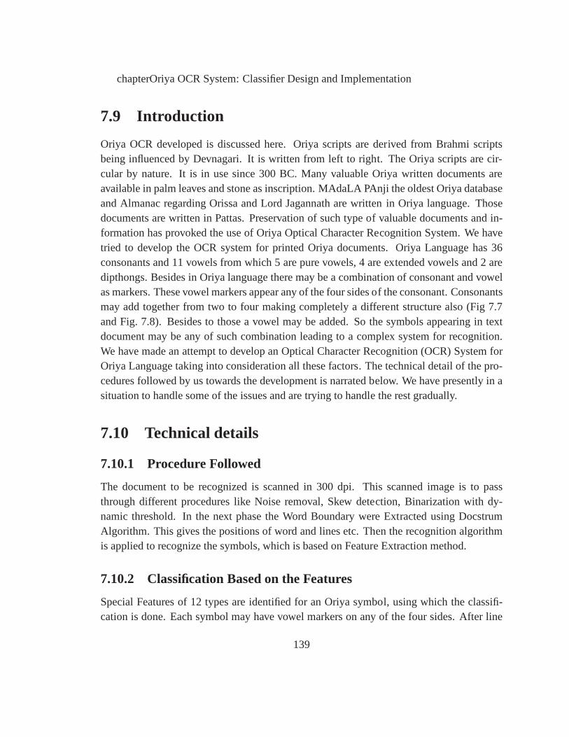
chapterOriya OCR System: Classifier Design and Implementation
7.9 Introduction
Oriya OCR developed is discussed here. Oriya scripts are derived from Brahmi scriptsbeing influenced by Devnagari. It is written from left to right. The Oriya scripts are cir-cular by nature. It is in use since 300 BC. Many valuable Oriyawritten documents areavailable in palm leaves and stone as inscription. MAdaLA PAnji the oldest Oriya databaseand Almanac regarding Orissa and Lord Jagannath are writtenin Oriya language. Thosedocuments are written in Pattas. Preservation of such type of valuable documents and in-formation has provoked the use of Oriya Optical Character Recognition System. We havetried to develop the OCR system for printed Oriya documents.Oriya Language has 36consonants and 11 vowels from which 5 are pure vowels, 4 are extended vowels and 2 aredipthongs. Besides in Oriya language there may be a combination of consonant and vowelas markers. These vowel markers appear any of the four sides of the consonant. Consonantsmay add together from two to four making completely a different structure also (Fig 7.7and Fig. 7.8). Besides to those a vowel may be added. So the symbols appearing in textdocument may be any of such combination leading to a complex system for recognition.We have made an attempt to develop an Optical Character Recognition (OCR) System forOriya Language taking into consideration all these factors. The technical detail of the pro-cedures followed by us towards the development is narrated below. We have presently in asituation to handle some of the issues and are trying to handle the rest gradually.
7.10 Technical details
7.10.1 Procedure Followed
The document to be recognized is scanned in 300 dpi. This scanned image is to passthrough different procedures like Noise removal, Skew detection, Binarization with dy-namic threshold. In the next phase the Word Boundary were Extracted using DocstrumAlgorithm. This gives the positions of word and lines etc. Then the recognition algorithmis applied to recognize the symbols, which is based on Feature Extraction method.
7.10.2 Classification Based on the Features
Special Features of 12 types are identified for an Oriya symbol, using which the classifi-cation is done. Each symbol may have vowel markers on any of the four sides. After line
139
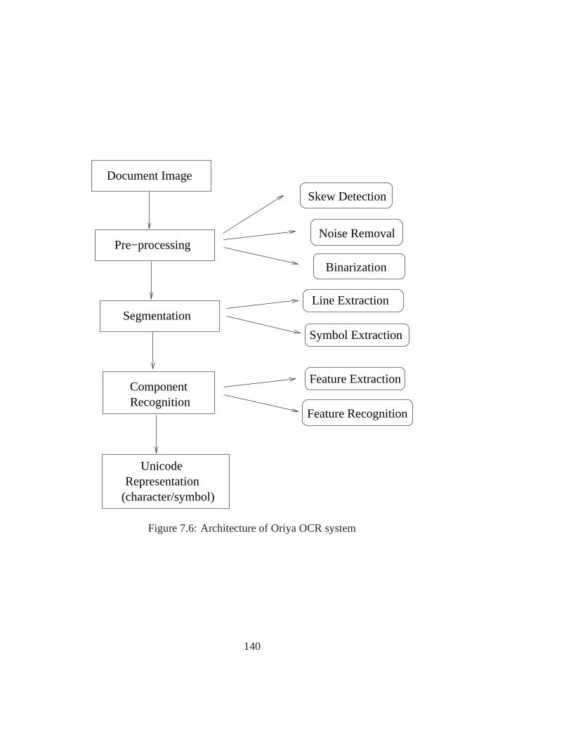
Document Image
Pre−processing
Segmentation
UnicodeRepresentation
(character/symbol)
ComponentRecognition
Skew Detection
Noise Removal
Binarization
Line Extraction
Symbol Extraction
Feature Extraction
Feature Recognition
Figure 7.6: Architecture of Oriya OCR system
140

Figure 7.7: An Oriya Document Image.
Figure 7.8: A degraded image with too many complexities.
extraction and word identification as per the histogram analysis the symbols are identifiedand feed for recognition. These individual symbols Characters are divided into three zonesi.e. the upper zone, middle zone and the lower zone. Taking into consideration all thesecharacteristics the classification was done. We have made a group of mainly three classes,then each one having subgroups. The classification goes on asper the appearance of thefeatures. Taking into consideration the Confusion Matrix for the Oriya scripts the Cluster-ing are done. Finally we reach at the leaf node of the decisiontree for a character throughnine levels. The presence of different features are recorded through a chain or combinationof binary codes To reach the leaf node after making a ground level recognition the nearestneighbors basing on which the clustering is done is also considered before the symbol isfinally dumped. To come to a conclusion we are suing the ID3 Algorithm where we arecalculating the entropy of the clusters of different paths.Finally the optimal one is selectedas the resultant one. A document of such type is difficult to recognize. It has misleadcharacters, Ligatures besides bad quality paper printed in.
141
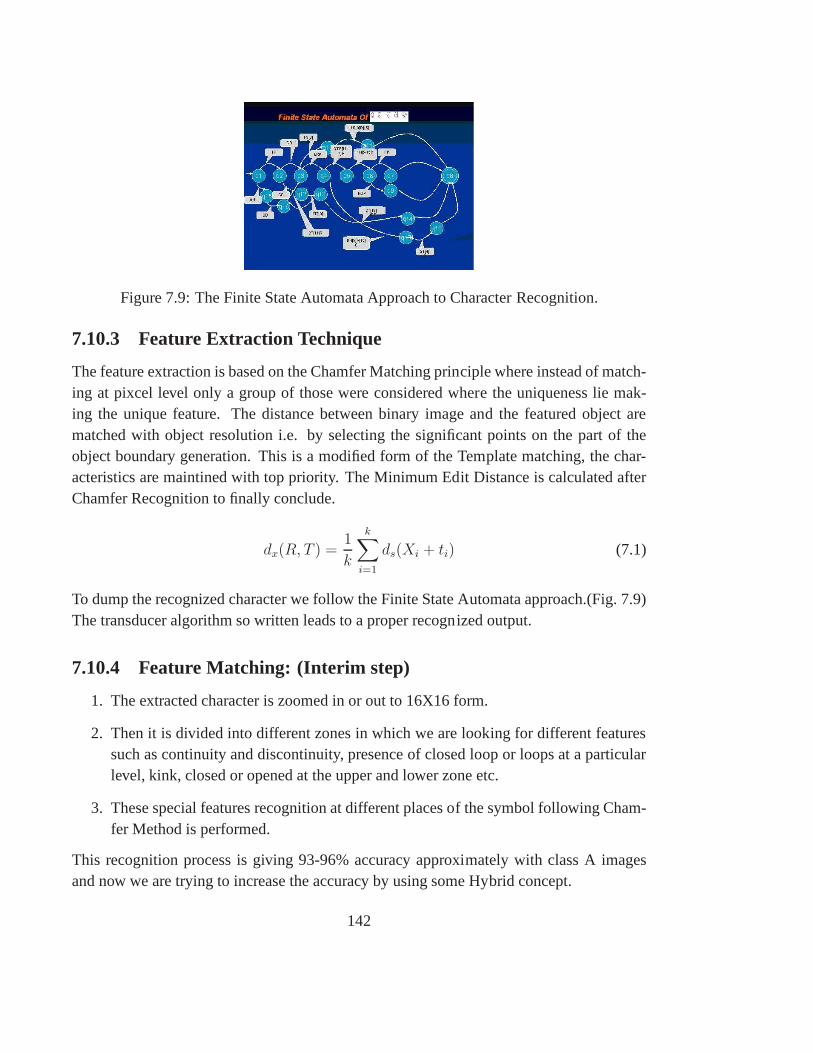
Figure 7.9: The Finite State Automata Approach to CharacterRecognition.
7.10.3 Feature Extraction Technique
The feature extraction is based on the Chamfer Matching principle where instead of match-ing at pixcel level only a group of those were considered where the uniqueness lie mak-ing the unique feature. The distance between binary image and the featured object arematched with object resolution i.e. by selecting the significant points on the part of theobject boundary generation. This is a modified form of the Template matching, the char-acteristics are maintined with top priority. The Minimum Edit Distance is calculated afterChamfer Recognition to finally conclude.
dx(R, T ) =1
k
k∑
i=1
ds(Xi + ti) (7.1)
To dump the recognized character we follow the Finite State Automata approach.(Fig. 7.9)The transducer algorithm so written leads to a proper recognized output.
7.10.4 Feature Matching: (Interim step)
1. The extracted character is zoomed in or out to 16X16 form.
2. Then it is divided into different zones in which we are looking for different featuressuch as continuity and discontinuity, presence of closed loop or loops at a particularlevel, kink, closed or opened at the upper and lower zone etc.
3. These special features recognition at different places of the symbol following Cham-fer Method is performed.
This recognition process is giving 93-96% accuracy approximately with class A imagesand now we are trying to increase the accuracy by using some Hybrid concept.
142
7.11 Future Work
Conjunct is a great problem for Oriya Language. Applying theChamfer Edit Distancecalculation based on the detailed feature extraction the accuracy rate for Conjuncts hasincreased. However we have also tried with Kohonen Neural Network an unsupervisedlearning system for the neurons where the recognition of conjuncts has improved to someextent.
We are also working with the Zernike Moment calculation where at around 25the roundof moment calculation the characters are reconstructed. Here we have tested with the nu-merals and other normal symbols. For too much distorted image document we are trying toimplement it. For Conjuncts and distorted image document the Zernike moment may cometo our help.
Presently we have started working on Convolution Neural Network (CNN) where therejection strategy may help us to find the exact output with a better precision. CNN is theNeural Network Model where unlike Kohonen it is supervised one where training of thepixcel sets is done. If the trained one is within the acceptable limit then we accept it as thecalculated result and if not we reject it. That is how it is better than the normal recognitionmethod. All these Neural Network methods lead to time complexity.
7.12 Issues in Oriya OCR
1. Degraded Images.
2. Bad Font Types through traditional Presses
3. Documents before 1990 are Lead Press printed.
4. Paper quality is too poor.
5. Conjuncts are not at all separable.
6. Vowel and consonant markers being on all side of the character, line separation andsegmentation are problem.
7. Even with good quality scanners of IIIT the line Segmentation algorithm for Anno-tation is not working. (Fig. 7.10)
8. Some document are so printed that symbol extraction with normal technique is diffi-cult. Better Binarization may be apoted. (Fig. 7.11)
143
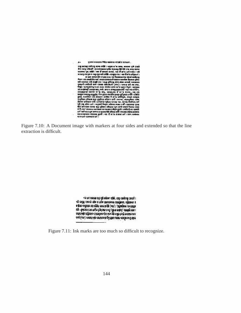
Figure 7.10: A Document image with markers at four sides and extended so that the lineextraction is difficult.
Figure 7.11: Ink marks are too much so difficult to recognize.
144

Chapter 8
Gurmukhi OCR System: ClassifierDesign and Implementation
8.1 Introduction
In this document, we present the complete Gurmukhi OCR system. Before the developmentof the present OCR, already a Gurmukhi OCR had been developedby us. But the OCR hadcertain limitations, such as it gave good results only on good quality images, it could nothandle broken and merged characters etc. To improve the existing OCR an analysis of themajor sources of errors in the OCR was carried out. It was found that broken characters andheadlines were one of the major cause of poor recognition, followed by multiple skewnessin text and merged characters. Wrong recognition by the OCR engine contributed to 40%of the errors. To improve the recognition, work was carried out in pre-processing stagefor handling the broken characters and multiple skewness, and multiple recognizers wereemployed to overcome the limitations of the current recognizer. The details are discussed infollowing sections. The flow diagram of the complete Gurmukhi OCR is shown in Fig. 8.1.Text in blue represents work already done, while text in red represents the work done incurrent phase. After digitization, skew correction and text segmentation, the next step isline extraction from the text image. Horizontal projectionof a document image is mostcommonly employed to extract the lines from the document. Ifthe lines are well separatedand not tilted, the horizontal projection will have well separated peaks and valleys. Thesevalleys are easily detected and used to determine the location of boundaries between lines.But this simple strategy when applied to Gurmukhi script fails in many cases and results inover segmentation or under segmentation. Over segmentation occurs when the white spacebreaks a text line into 2 or more horizontal text strips (Textline 1 in Fig. 8.2). In printed
145
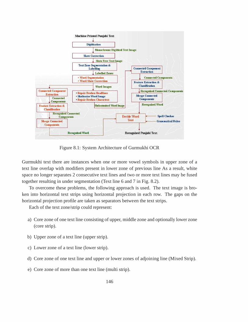
Figure 8.1: System Architecture of Gurmukhi OCR
Gurmukhi text there are instances when one or more vowel symbols in upper zone of atext line overlap with modifiers present in lower zone of previous line As a result, whitespace no longer separates 2 consecutive text lines and two ormore text lines may be fusedtogether resulting in under segmentation (Text line 6 and 7 in Fig. 8.2).
To overcome these problems, the following approach is used.The text image is bro-ken into horizontal text strips using horizontal projection in each row. The gaps on thehorizontal projection profile are taken as separators between the text strips.
Each of the text zone/strip could represent:
a) Core zone of one text line consisting of upper, middle zoneand optionally lower zone(core strip).
b) Upper zone of a text line (upper strip).
c) Lower zone of a text line (lower strip).
d) Core zone of one text line and upper or lower zones of adjoining line (Mixed Strip).
e) Core zone of more than one text line (multi strip).
146
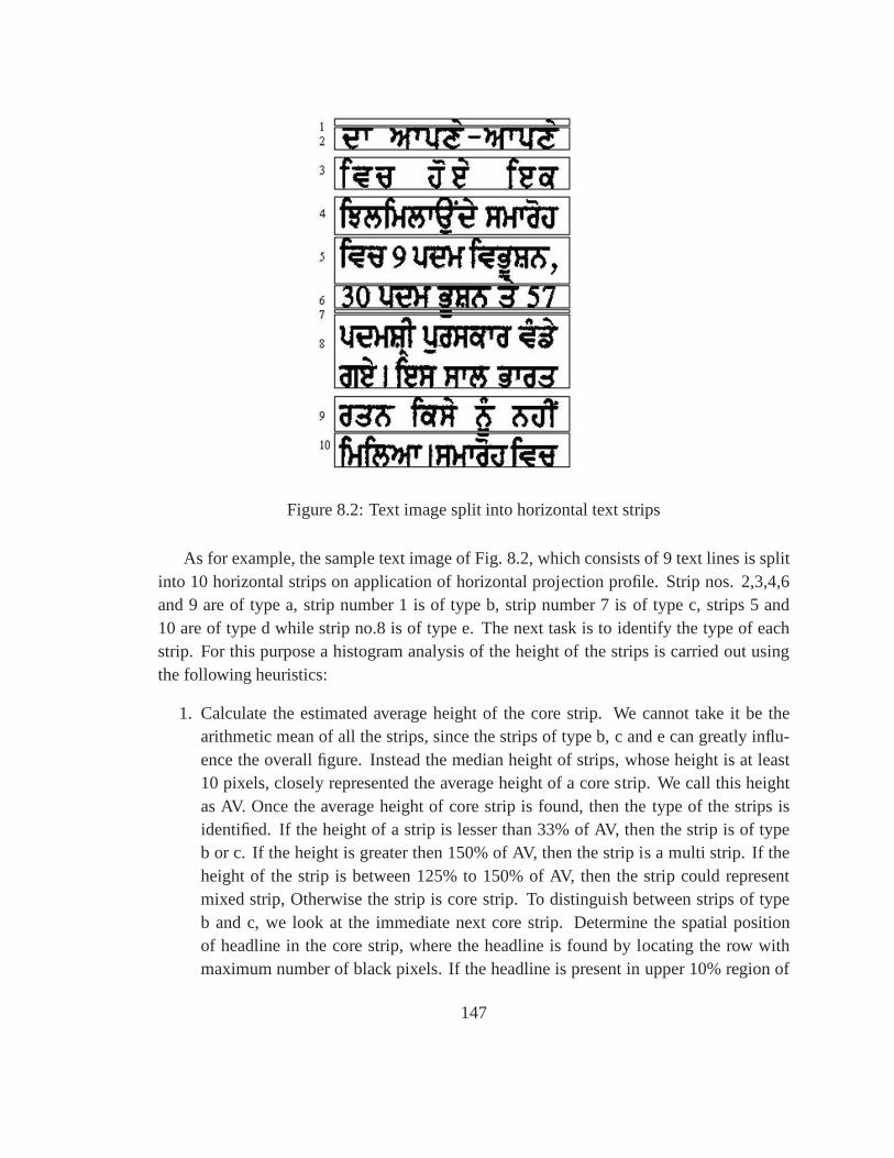
Figure 8.2: Text image split into horizontal text strips
As for example, the sample text image of Fig. 8.2, which consists of 9 text lines is splitinto 10 horizontal strips on application of horizontal projection profile. Strip nos. 2,3,4,6and 9 are of type a, strip number 1 is of type b, strip number 7 isof type c, strips 5 and10 are of type d while strip no.8 is of type e. The next task is toidentify the type of eachstrip. For this purpose a histogram analysis of the height ofthe strips is carried out usingthe following heuristics:
1. Calculate the estimated average height of the core strip.We cannot take it be thearithmetic mean of all the strips, since the strips of type b,c and e can greatly influ-ence the overall figure. Instead the median height of strips,whose height is at least10 pixels, closely represented the average height of a core strip. We call this heightas AV. Once the average height of core strip is found, then thetype of the strips isidentified. If the height of a strip is lesser than 33% of AV, then the strip is of typeb or c. If the height is greater then 150% of AV, then the strip is a multi strip. If theheight of the strip is between 125% to 150% of AV, then the strip could representmixed strip, Otherwise the strip is core strip. To distinguish between strips of typeb and c, we look at the immediate next core strip. Determine the spatial positionof headline in the core strip, where the headline is found by locating the row withmaximum number of black pixels. If the headline is present inupper 10% region of
147
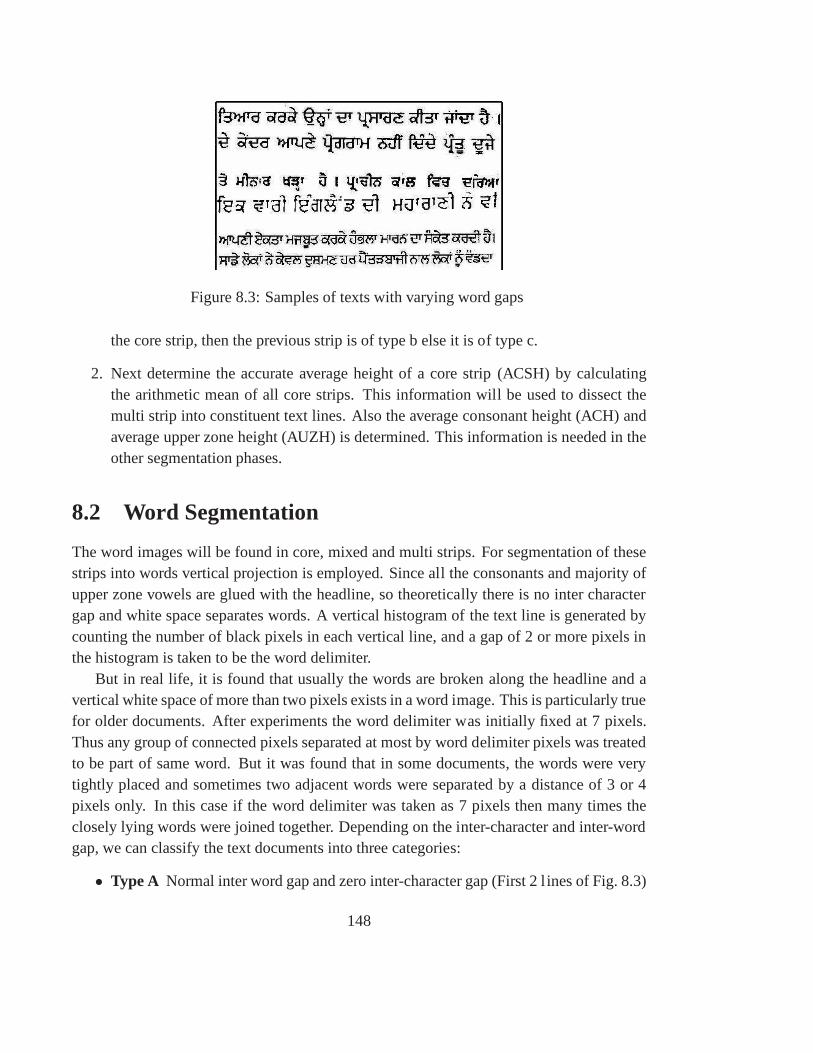
Figure 8.3: Samples of texts with varying word gaps
the core strip, then the previous strip is of type b else it is of type c.
2. Next determine the accurate average height of a core strip(ACSH) by calculatingthe arithmetic mean of all core strips. This information will be used to dissect themulti strip into constituent text lines. Also the average consonant height (ACH) andaverage upper zone height (AUZH) is determined. This information is needed in theother segmentation phases.
8.2 Word Segmentation
The word images will be found in core, mixed and multi strips.For segmentation of thesestrips into words vertical projection is employed. Since all the consonants and majority ofupper zone vowels are glued with the headline, so theoretically there is no inter charactergap and white space separates words. A vertical histogram ofthe text line is generated bycounting the number of black pixels in each vertical line, and a gap of 2 or more pixels inthe histogram is taken to be the word delimiter.
But in real life, it is found that usually the words are brokenalong the headline and avertical white space of more than two pixels exists in a word image. This is particularly truefor older documents. After experiments the word delimiter was initially fixed at 7 pixels.Thus any group of connected pixels separated at most by word delimiter pixels was treatedto be part of same word. But it was found that in some documents, the words were verytightly placed and sometimes two adjacent words were separated by a distance of 3 or 4pixels only. In this case if the word delimiter was taken as 7 pixels then many times theclosely lying words were joined together. Depending on the inter-character and inter-wordgap, we can classify the text documents into three categories:
• Type A Normal inter word gap and zero inter-character gap (First 2 lines of Fig. 8.3)
148
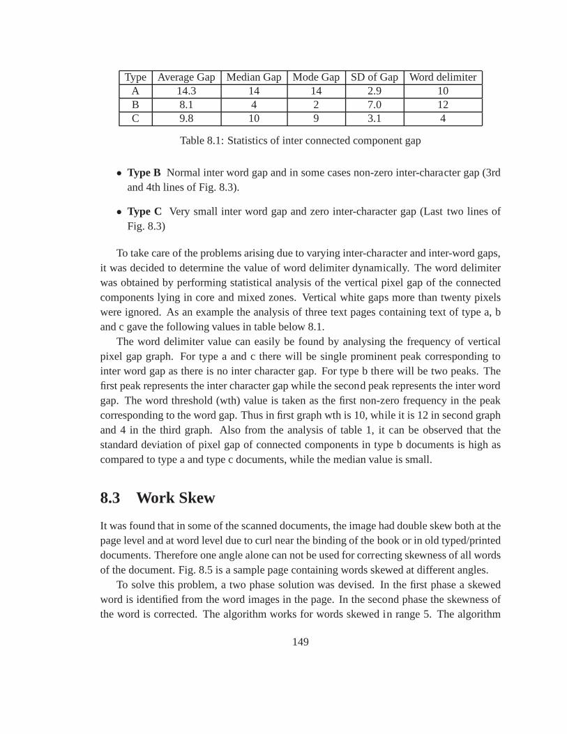
Type Average Gap Median Gap Mode Gap SD of Gap Word delimiterA 14.3 14 14 2.9 10B 8.1 4 2 7.0 12C 9.8 10 9 3.1 4
Table 8.1: Statistics of inter connected component gap
• Type B Normal inter word gap and in some cases non-zero inter-character gap (3rdand 4th lines of Fig. 8.3).
• Type C Very small inter word gap and zero inter-character gap (Lasttwo lines ofFig. 8.3)
To take care of the problems arising due to varying inter-character and inter-word gaps,it was decided to determine the value of word delimiter dynamically. The word delimiterwas obtained by performing statistical analysis of the vertical pixel gap of the connectedcomponents lying in core and mixed zones. Vertical white gaps more than twenty pixelswere ignored. As an example the analysis of three text pages containing text of type a, band c gave the following values in table below 8.1.
The word delimiter value can easily be found by analysing thefrequency of verticalpixel gap graph. For type a and c there will be single prominent peak corresponding tointer word gap as there is no inter character gap. For type b there will be two peaks. Thefirst peak represents the inter character gap while the second peak represents the inter wordgap. The word threshold (wth) value is taken as the first non-zero frequency in the peakcorresponding to the word gap. Thus in first graph wth is 10, while it is 12 in second graphand 4 in the third graph. Also from the analysis of table 1, it can be observed that thestandard deviation of pixel gap of connected components in type b documents is high ascompared to type a and type c documents, while the median value is small.
8.3 Work Skew
It was found that in some of the scanned documents, the image had double skew both at thepage level and at word level due to curl near the binding of thebook or in old typed/printeddocuments. Therefore one angle alone can not be used for correcting skewness of all wordsof the document. Fig. 8.5 is a sample page containing words skewed at different angles.
To solve this problem, a two phase solution was devised. In the first phase a skewedword is identified from the word images in the page. In the second phase the skewness ofthe word is corrected. The algorithm works for words skewed in range 5. The algorithm
149
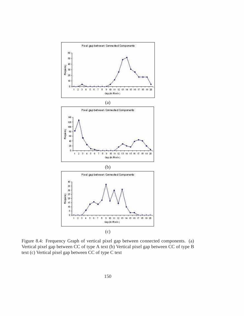
(a)
(b)
(c)
Figure 8.4: Frequency Graph of vertical pixel gap between connected components. (a)Vertical pixel gap between CC of type A text (b) Vertical pixel gap between CC of type Btext (c) Vertical pixel gap between CC of type C text
150
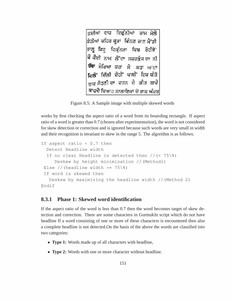
Figure 8.5: A Sample image with multiple skewed words
works by first checking the aspect ratio of a word from its bounding rectangle. If aspectratio of a word is greater than 0.7 (chosen after experimentation), the word is not consideredfor skew detection or correction and is ignored because suchwords are very small in widthand their recognition is invariant to skew in the range 5. Thealgorithm is as follows:
If aspect ratio < 0.7 then
Detect Headline width
If no clear Headline is detected then //(< 75\%)
Deskew by height minimization //(Method1)
Else //(headline width >= 75\%)
If word is skewed then
Deskew by maximizing the headline width //(Method 2)
Endif
8.3.1 Phase 1: Skewed word identification
If the aspect ratio of the word is less than 0.7 then the word becomes target of skew de-tection and correction. There are some characters in Gurmukhi script which do not haveheadline If a word consisting of one or more of these characters is encountered then alsoa complete headline is not detected.On the basis of the abovethe words are classified intotwo categories:
• Type 1: Words made up of all characters with headline,
• Type 2: Words with one or more character without headline.
151
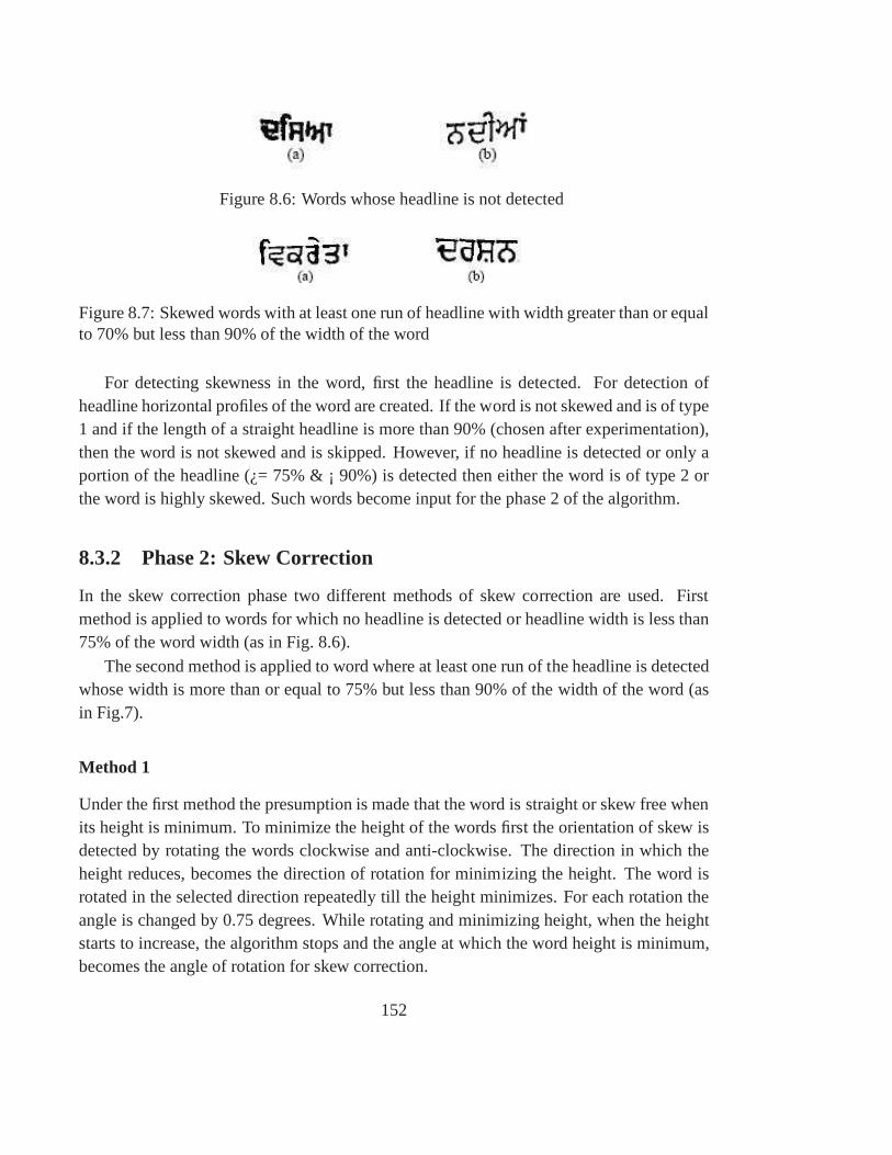
Figure 8.6: Words whose headline is not detected
Figure 8.7: Skewed words with at least one run of headline with width greater than or equalto 70% but less than 90% of the width of the word
For detecting skewness in the word, first the headline is detected. For detection ofheadline horizontal profiles of the word are created. If the word is not skewed and is of type1 and if the length of a straight headline is more than 90% (chosen after experimentation),then the word is not skewed and is skipped. However, if no headline is detected or only aportion of the headline (¿= 75% & ¡ 90%) is detected then either the word is of type 2 orthe word is highly skewed. Such words become input for the phase 2 of the algorithm.
8.3.2 Phase 2: Skew Correction
In the skew correction phase two different methods of skew correction are used. Firstmethod is applied to words for which no headline is detected or headline width is less than75% of the word width (as in Fig. 8.6).
The second method is applied to word where at least one run of the headline is detectedwhose width is more than or equal to 75% but less than 90% of thewidth of the word (asin Fig.7).
Method 1
Under the first method the presumption is made that the word isstraight or skew free whenits height is minimum. To minimize the height of the words first the orientation of skew isdetected by rotating the words clockwise and anti-clockwise. The direction in which theheight reduces, becomes the direction of rotation for minimizing the height. The word isrotated in the selected direction repeatedly till the height minimizes. For each rotation theangle is changed by 0.75 degrees. While rotating and minimizing height, when the heightstarts to increase, the algorithm stops and the angle at which the word height is minimum,becomes the angle of rotation for skew correction.
152
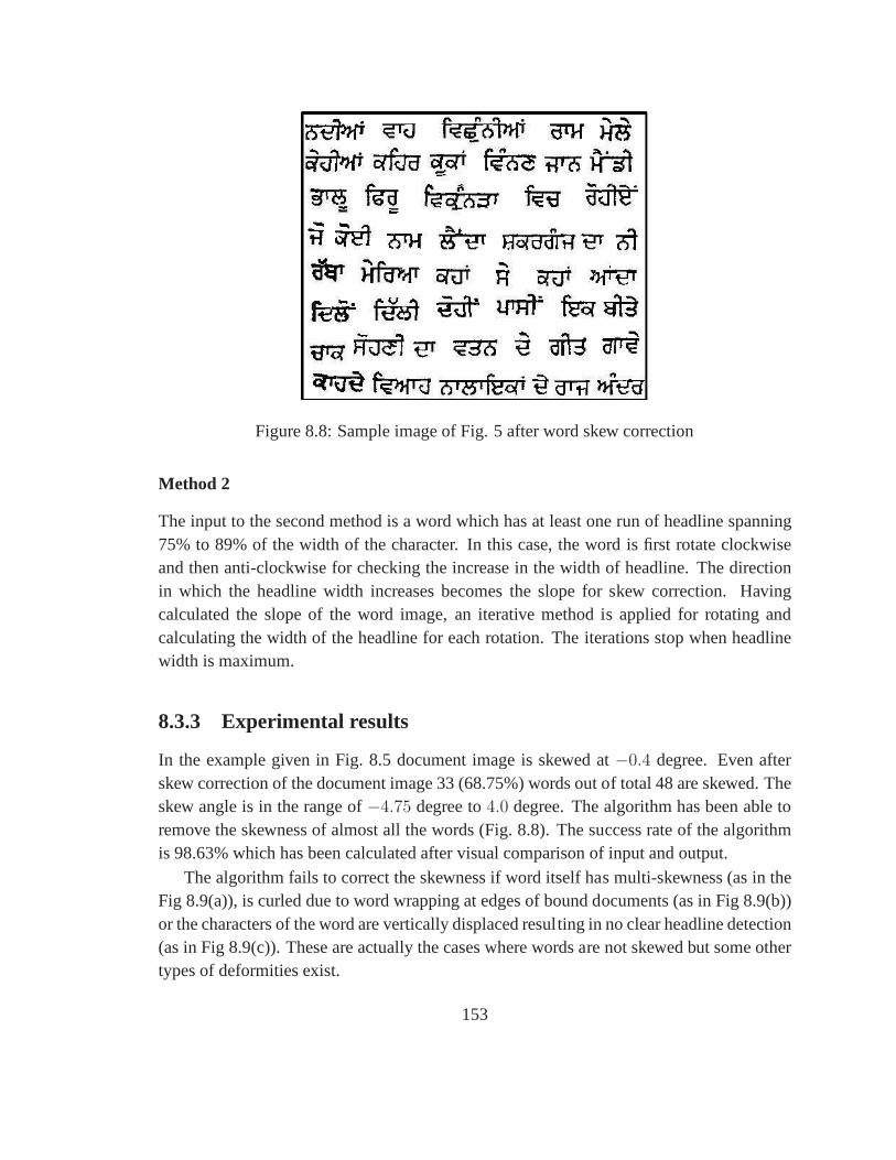
Figure 8.8: Sample image of Fig. 5 after word skew correction
Method 2
The input to the second method is a word which has at least one run of headline spanning75% to 89% of the width of the character. In this case, the wordis first rotate clockwiseand then anti-clockwise for checking the increase in the width of headline. The directionin which the headline width increases becomes the slope for skew correction. Havingcalculated the slope of the word image, an iterative method is applied for rotating andcalculating the width of the headline for each rotation. Theiterations stop when headlinewidth is maximum.
8.3.3 Experimental results
In the example given in Fig. 8.5 document image is skewed at−0.4 degree. Even afterskew correction of the document image 33 (68.75%) words out of total 48 are skewed. Theskew angle is in the range of−4.75 degree to4.0 degree. The algorithm has been able toremove the skewness of almost all the words (Fig. 8.8). The success rate of the algorithmis 98.63% which has been calculated after visual comparisonof input and output.
The algorithm fails to correct the skewness if word itself has multi-skewness (as in theFig 8.9(a)), is curled due to word wrapping at edges of bound documents (as in Fig 8.9(b))or the characters of the word are vertically displaced resulting in no clear headline detection(as in Fig 8.9(c)). These are actually the cases where words are not skewed but some othertypes of deformities exist.
153

Figure 8.9: Failure cases for word skew removal
(a) (b)
Figure 8.10: a) A word with broken headlines b) After repair
8.4 Repairing the Word Shape
Some preprocessing operations have to be performed on the word images, before they aresent for character segmentation. In older texts, the word images are frequently broken alongthe headlines as well at character level. So it is necessary to repair the word shapes. In aGurmukhi word the middle zone characters are glued along theheadline. The charactersegmentor expects the middle zone characters to be touchingthe headline, with no verti-cal inter-character gap. But sometimes, the headline is broken and the characters are notaligned along the y-axis as a result the word image is split into a group of single or multiplecharacters (Fig. 8.10(a). This creates problem for the character segmentor as it becomesdifficult to identify the position of the headline and the components lying above and belowit. Thus it becomes necessary to join the broken headlines and align the headline of thecharacters of the word by displacing the character images along the y-axis (Fig 8.10(b).This is achieved as follow:
1. Determine the row in the word image corresponding to the word headline (WHL) inthe upper half of the word image satisfying one or both of the following criteria:
• Row with maximum horizontal span of black pixels.
• Row having maximum number of black pixel count.
2. Decompose the word image into connected components (CCs)separated by verticalwhite space. Each of these CC could represent a group of one ormore characters. For
154
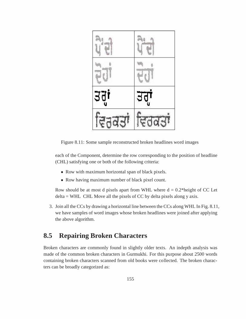
Figure 8.11: Some sample reconstructed broken headlines word images
each of the Component, determine the row corresponding to the position of headline(CHL) satisfying one or both of the following criteria:
• Row with maximum horizontal span of black pixels.
• Row having maximum number of black pixel count.
Row should be at most d pixels apart from WHL where d = 0.2*height of CC Letdelta = WHL CHL Move all the pixels of CC by delta pixels along yaxis.
3. Join all the CCs by drawing a horizontal line between the CCs along WHL In Fig. 8.11,we have samples of word images whose broken headlines were joined after applyingthe above algorithm.
8.5 Repairing Broken Characters
Broken characters are commonly found in slightly older texts. An indepth analysis wasmade of the common broken characters in Gurmukhi. For this purpose about 2500 wordscontaining broken characters scanned from old books were collected. The broken charac-ters can be broadly categorized as:
155
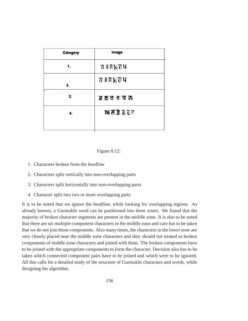
Figure 8.12:
1. Characters broken from the headline
2. Characters split vertically into non-overlapping parts
3. Characters split horizontally into non-overlapping parts
4. Character split into two or more overlapping parts
It is to be noted that we ignore the headline, while looking for overlapping regions. Asalready known, a Gurmukhi word can be partitioned into threezones. We found that themajority of broken character segments are present in the middle zone. It is also to be notedthat there are six multiple component characters in the middle zone and care has to be takenthat we do not join those components. Also many times, the characters in the lower zone arevery closely placed near the middle zone characters and theyshould not treated as brokencomponents of middle zone characters and joined with them. The broken components haveto be joined with the appropriate components to form the character. Decision also has to betaken which connected component pairs have to be joined and which were to be ignored.All this calls for a detailed study of the structure of Gurmukhi characters and words, whiledesigning the algorithm.
156
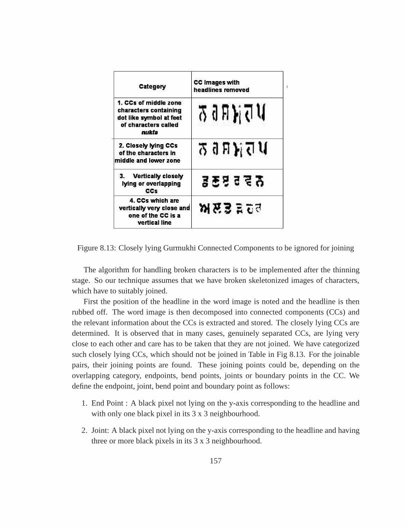
Figure 8.13: Closely lying Gurmukhi Connected Components to be ignored for joining
The algorithm for handling broken characters is to be implemented after the thinningstage. So our technique assumes that we have broken skeletonized images of characters,which have to suitably joined.
First the position of the headline in the word image is noted and the headline is thenrubbed off. The word image is then decomposed into connectedcomponents (CCs) andthe relevant information about the CCs is extracted and stored. The closely lying CCs aredetermined. It is observed that in many cases, genuinely separated CCs, are lying veryclose to each other and care has to be taken that they are not joined. We have categorizedsuch closely lying CCs, which should not be joined in Table inFig 8.13. For the joinablepairs, their joining points are found. These joining pointscould be, depending on theoverlapping category, endpoints, bend points, joints or boundary points in the CC. Wedefine the endpoint, joint, bend point and boundary point as follows:
1. End Point : A black pixel not lying on the y-axis corresponding to the headline andwith only one black pixel in its 3 x 3 neighbourhood.
2. Joint: A black pixel not lying on the y-axis correspondingto the headline and havingthree or more black pixels in its 3 x 3 neighbourhood.
157
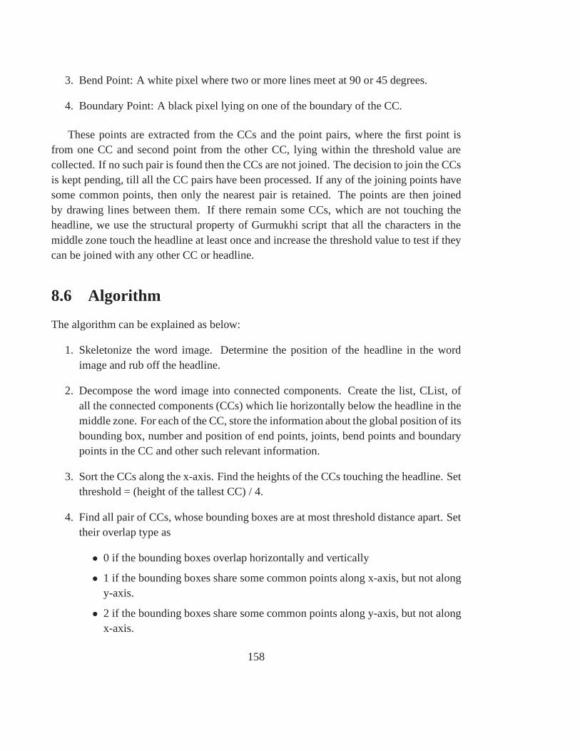
3. Bend Point: A white pixel where two or more lines meet at 90 or 45 degrees.
4. Boundary Point: A black pixel lying on one of the boundary of the CC.
These points are extracted from the CCs and the point pairs, where the first point isfrom one CC and second point from the other CC, lying within the threshold value arecollected. If no such pair is found then the CCs are not joined. The decision to join the CCsis kept pending, till all the CC pairs have been processed. Ifany of the joining points havesome common points, then only the nearest pair is retained. The points are then joinedby drawing lines between them. If there remain some CCs, which are not touching theheadline, we use the structural property of Gurmukhi scriptthat all the characters in themiddle zone touch the headline at least once and increase thethreshold value to test if theycan be joined with any other CC or headline.
8.6 Algorithm
The algorithm can be explained as below:
1. Skeletonize the word image. Determine the position of theheadline in the wordimage and rub off the headline.
2. Decompose the word image into connected components. Create the list, CList, ofall the connected components (CCs) which lie horizontally below the headline in themiddle zone. For each of the CC, store the information about the global position of itsbounding box, number and position of end points, joints, bend points and boundarypoints in the CC and other such relevant information.
3. Sort the CCs along the x-axis. Find the heights of the CCs touching the headline. Setthreshold = (height of the tallest CC) / 4.
4. Find all pair of CCs, whose bounding boxes are at most threshold distance apart. Settheir overlap type as
• 0 if the bounding boxes overlap horizontally and vertically
• 1 if the bounding boxes share some common points along x-axis, but not alongy-axis.
• 2 if the bounding boxes share some common points along y-axis, but not alongx-axis.
158

• 3 if the bounding boxes do not share any common points in x or y axis.
5. If for any pair of CCs, CC1 and CC2, if CC1 lies in the lower quarter of the wordimage along y-axis, check that:
• The minimum value of bounding box of CC1 along y-axis should not be greaterthan the median height of the CCs touching the headline.
• The area of CC1 should be at least 12 pixels.
• If the overlap type is 0, then CC1 should not lie in the middle or left of CC2.
If any of the above condition is false, remove the pair from the list. This is to avoidjoining the nukta signs and the characters lying in lower zone with the middle zonecharacters (Category 1 and 2 of Table in Fig 8.12).
6. If overlap type is 0, set thresh = 1.25*threshold. Let S1 = Set of all endpoints, bendpoints and joints in CC1. Let S2 = Set of all endpoints, bend points and joints in CC2.Find C= Set of all pairs of points from S1 and S2 which lie within thresh distance. Iffor any pair, their bounding boxes overlap, retain the smaller distance pair and deletethe other pair to avoid creation of cycles.
7. If overlap type is 1 or 3, set thresh = threshold. Assume CC1is nearer to headline.Let S1 = Set of all endpoints, bendpoints, joints and boundary points lying along thelower horizontal boundary of the bounding box of CC1. Let S2 =Set of all endpoints,bend points, joints and boundary points lying along the upper horizontal boundary ofthe bounding box of CC2. Find C= Set of all pairs of points fromS1 and S2 whichlie within thresh distance.
8. If overlap type is 2, set thresh = threshold. Assume CC1 occurs before CC2 in thesorting order along x-axis. If CC1 is a vertical line or the width to height ratio ofthe bounding box formed by joining CC1 and CC2 is greater than1.25 then ignorethis pair for merging. This is to take care that the closely lying characters are notmerged together (Category 3 and 4 Table in Fig. 8.12). Let S1 =Set of all endpoints,bendpoints, joints and boundary points lying along the right vertical boundary of thebounding box. Let S2 = Set of all endpoints, bend points and joints and boundarypoints lying along the left vertical boundary of the bounding box of CC2. If CC2 isa vertical line then exclude the joints and boundary points from S1. This is to avoidjoining CCs similar to first and third pairs of CCs of category4 in Table in Fig. 8.12 ,as their nearest joining points lying within the threshold are on boundary or on joints.
159

Find C= Set of all pairs of points from S1 and S2 which lie within thresh. If both thepoints in a pair are boundary points, remove that pair.
9. Examine all the candidate pairs in set C. If any pair has a common co-ordinate point,retain the one having smaller distance.
10. At the end join all the candidate pairs in set C by drawing astraight line betweenthem. Update CList, the list of Connected Components, by replacing the CCs whichhave been joined with the new merged CC.
11. Let SList be the sublist of CList containing connected components not touching theheadline. If SList is not empty, then add the skeletonized image of headline to CList.
12. If SList empty then Stop, else Set thresh = 1.5 * threshold. Repeat the steps 5 to 11and then stop. Instead of taking both pairs of CCs from Clist,one element is fromCList and second from SList. This is to ensure the Gurmukhi Script property that allthe characters in the middle zone, touch the headline at least once. So if we find a CCnot touching the headline, then it is a candidate for joiningwith either the headlineor some other CC which is touching the headline.
8.6.1 Experiments
The algorithm was tested on a set of 2500 words containing broken characters and in 82.3%of cases, the broken components were correctly joined together to form a recognizable unit,while in 4.9% of cases, the components were wrongly joined and in 12.8% of cases thebroken components were not joined with any other component.Some sample images areshown in Fig. 8.11. The different stages through which an image passes are shown in theFig. 8.15. The first stage is the extracted word image. In the second stage the image’sheadline is corrected. The image is skeletonized in the third stage and in the last stage thebroken characters in the image are repaired and the headlinesmoothened.
For recognition, the word image is fed to different feature extraction and classifica-tion modules and their recognition results are combined to get the final recognized text.The input images for the features extractors are original image(OI, Fig 8.15(a)), imageafter repairing the broken headline and character(RI, Fig 8.15(b)) and thinned image(TI,Fig 8.15(c)).
For OI and RI images, the following features are used:
• Structural Features
– Presence of sidebar
160
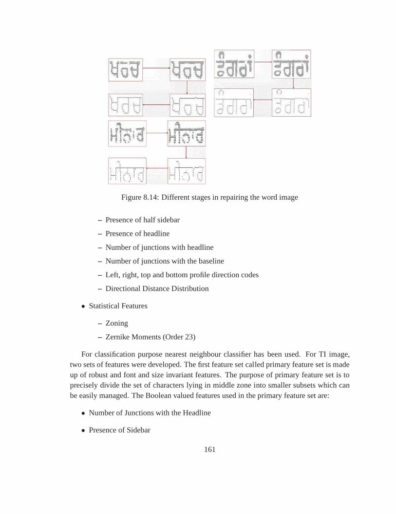
Figure 8.14: Different stages in repairing the word image
– Presence of half sidebar
– Presence of headline
– Number of junctions with headline
– Number of junctions with the baseline
– Left, right, top and bottom profile direction codes
– Directional Distance Distribution
• Statistical Features
– Zoning
– Zernike Moments (Order 23)
For classification purpose nearest neighbour classifier hasbeen used. For TI image,two sets of features were developed. The first feature set called primary feature set is madeup of robust and font and size invariant features. The purpose of primary feature set is toprecisely divide the set of characters lying in middle zone into smaller subsets which canbe easily managed. The Boolean valued features used in the primary feature set are:
• Number of Junctions with the Headline
• Presence of Sidebar
161
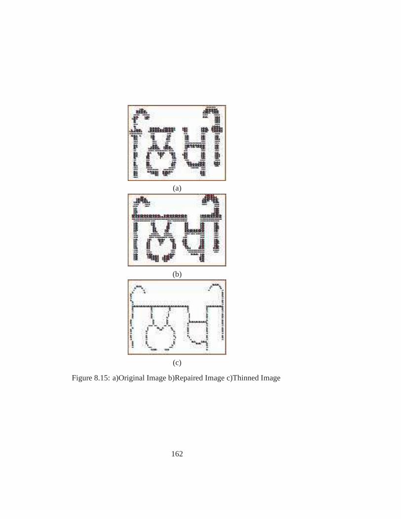
(a)
(b)
(c)
Figure 8.15: a)Original Image b)Repaired Image c)Thinned Image
162

• Presence of a Loop
• No Loop Formed with Headline
The second feature set, called secondary feature set, is a combination of local and globalfeatures, which are aimed to capture the geometrical and topological features of the charac-ters and efficiently distinguish and identify the characterfrom a small subset of characters.The Secondary Feature Set consists of following features:
• Number of Endpoints and their Location
• Number of Junctions and their Location
• Horizontal Projection Count
• Left and Right Projection Profiles
• Right Profile Depth
• Left Profile Upper Depth
• Left Profile Lower Depth
• Left and Right Profile Direction Code
• Aspect Ratio
• Distribution of Black Pixels about the Horizontal mid-line
For classification purpose, binary tree classifier and nearest neighbour classifiers have beenused. The output of all the three classifiers is then combinedto get the final output asoutlined in following algorithm. To compare the results, wehave used a set of unigramsextracted from a 10 million word Punjabi corpus.
Input
1. Recognized words from TI, RI and OI images. (w1, w2 and w3 respectively)
2. Set of Unigrams extracted from a 10 million word Punjabi corpus. (UG)
Output
The output is a Recognized word.
163
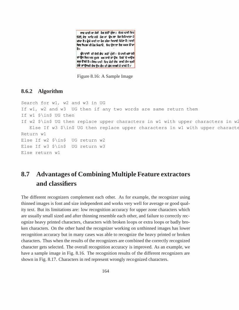
Figure 8.16: A Sample Image
8.6.2 Algorithm
Search for w1, w2 and w3 in UG
If w1, w2 and w3 UG then if any two words are same return them
If w1 $\in$ UG then
If w2 $\in$ UG then replace upper characters in w1 with upper characters in w2
Else If w3 $\in$ UG then replace upper characters in w1 with upper characters
Return w1
Else If w2 $\in$ UG return w2
Else If w3 $\in$ UG return w3
Else return w1
8.7 Advantages of Combining Multiple Feature extractorsand classifiers
The different recognizers complement each other. As for example, the recognizer usingthinned images is font and size independent and works very well for average or good qual-ity text. But its limitations are: low recognition accuracyfor upper zone characters whichare usually small sized and after thinning resemble each other, and failure to correctly rec-ognize heavy printed characters, characters with broken loops or extra loops or badly bro-ken characters. On the other hand the recognizer working on unthinned images has lowerrecognition accuracy but in many cases was able to recognizethe heavy printed or brokencharacters. Thus when the results of the recognizers are combined the correctly recognizedcharacter gets selected. The overall recognition accuracyis improved. As an example, wehave a sample image in Fig. 8.16. The recognition results of the different recognizers areshown in Fig. 8.17. Characters in red represent wrongly recognized characters.
164
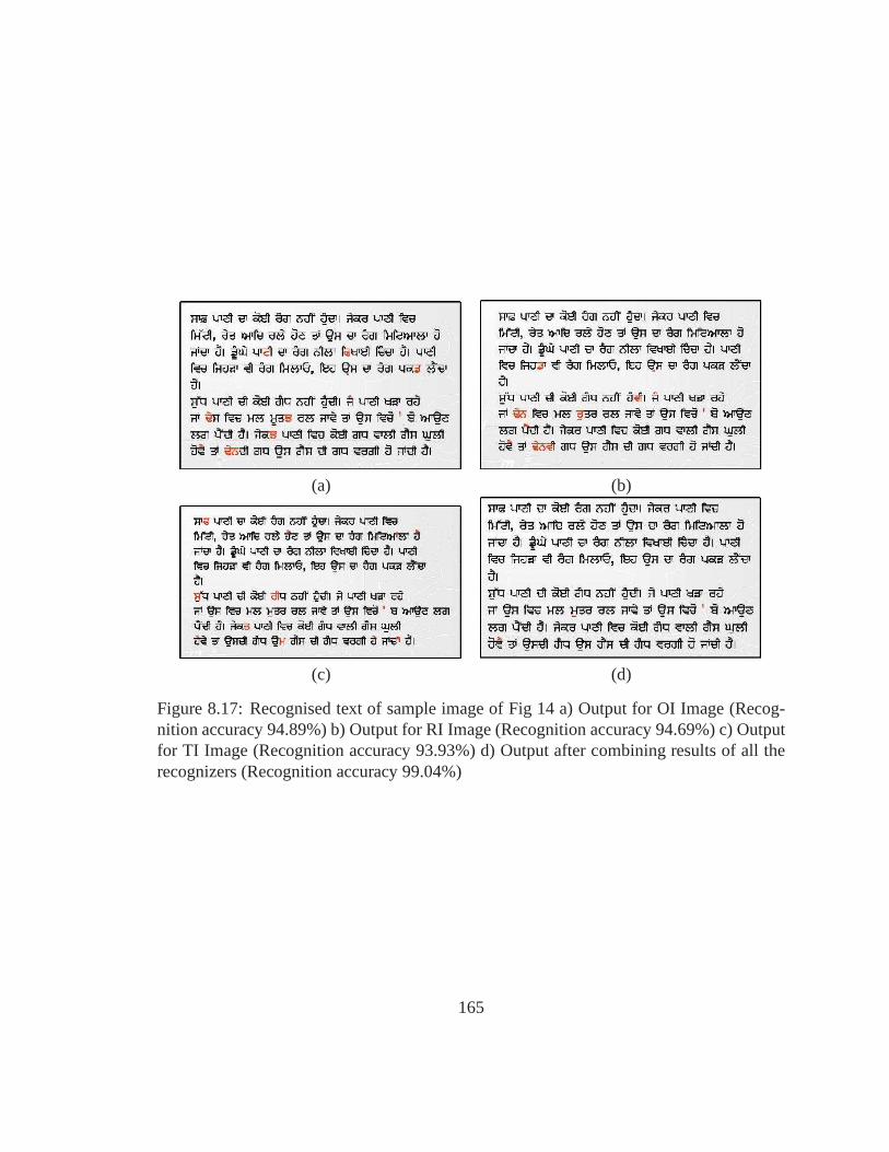
(a) (b)
(c) (d)
Figure 8.17: Recognised text of sample image of Fig 14 a) Output for OI Image (Recog-nition accuracy 94.89%) b) Output for RI Image (Recognitionaccuracy 94.69%) c) Outputfor TI Image (Recognition accuracy 93.93%) d) Output after combining results of all therecognizers (Recognition accuracy 99.04%)
165
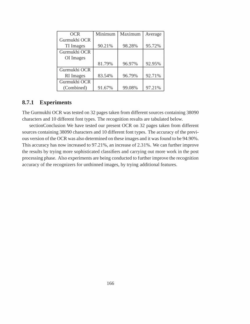
OCR Minimum Maximum AverageGurmukhi OCR
TI Images 90.21% 98.28% 95.72%Gurmukhi OCR
OI Images81.79% 96.97% 92.95%
Gurmukhi OCRRI Images 83.54% 96.79% 92.71%
Gurmukhi OCR(Combined) 91.67% 99.08% 97.21%
8.7.1 Experiments
The Gurmukhi OCR was tested on 32 pages taken from different sources containing 38090characters and 10 different font types. The recognition results are tabulated below.
sectionConclusion We have tested our present OCR on 32 pagestaken from differentsources containing 38090 characters and 10 different font types. The accuracy of the previ-ous version of the OCR was also determined on these images andit was found to be 94.90%.This accuracy has now increased to 97.21%, an increase of 2.31%. We can further improvethe results by trying more sophisticated classifiers and carrying out more work in the postprocessing phase. Also experiments are being conducted to further improve the recognitionaccuracy of the recognizers for unthinned images, by tryingadditional features.
166

Chapter 9
Gujarati Script Dependent Module forOCR
Target Set for June 2008 : Alpha Version of script dependent module.
9.1 Status of Development :
The major tasks carried out during this phase of developmentare fine tuning of zone sepa-ratio n algorithm, development of recognition engine with various features extraction tech-niques. Fringe Map, Discrete Cosine Transform Coefficientsand Zernike Moment(Codefrom University of Hyderabad) have been tested. Other contributions on the consortiumsite like Convolution Neural Network based binary classifier from UOH were also tested.The details of the entire approach is as follows :
• Input : Binarized Image of a paragraph
• Script Specific Document Analysis
– Line Separation : Routines contributed by ISI Kolkata.
– Word Separation : Analyzing vertical projection of the line.
• Zone Boundary Detection : The zone separation is now done at two levels lineand word. It takes an array of connected components and returns a two elementarray storing the line numbers where the zone boundary is identified. The approchfollowed to decide the final zone boundary is as described in [40].
167
• Recognizable Unit :After the zone boundaries are fixed, only those connected com-ponents which are having their height more than the height ofmiddle zone are fur-there analysed for extracting out connected component in each of the zones and oth-ers based on their location classified as upper, middel or lower zone components.
Each of the connected components is then scaled to a uniform size of 32×32 pixelsand these scaled connected components are then recognized.In order to avoid noise,that might be left out at the time binarization or may be generated due to segme-nation of baseline glyph at the time of zone boundary detection, all the connectedcomponents where number of rows or number of columns are lessthan a pre-decidedthreshold(currently 3) than those components are not scaled and discarded.
• RecognitionInput : A 32×32 binary matrix
• Feature Extraction Three freature extraction Techniques have been used.
1. Fringe Map : Created by replacing each pixels from its nearest black pixel in4-neighbor sense.No. of Features : 1024 (Integers)
2. Discrete Cosine Transfrom : 2D discrete cosine transformof 32×32 image iscomputed and coefficients are extracted in zig-zag order.No. of Features : 80
3. Zernike Moments (Code from UOH): 32×32 image is subected to routine con-tributed by Univ. of HyderabadNo.of Features : 72
4. Zone Information : Along with other features we use zone information of theconnected component to reduce the search.
• Classifier Tested the code(from UOH) of Binary Classifier based on ConvolutionalNeural Network. At pressent the recognition engine uses nearest neighbour classi-fier. In addition to this, the codes that will be uploaded by IIT Hyderabad (SVM),Univ. Of Hyderabad (Multiclass CNN) and IIIT Alahabad(ADA)will also be in-corporated and results will be obtained. Expected to complete the development ofGeneral Regression Neural Network and test it by June end.
• Text Generation Based on relative location in the document, recognized connectedcomponents are grouped in to a so called glyph cluster (set ofglyphs representing aC*CV combination). The non-uniform way of formulating the character across the
168
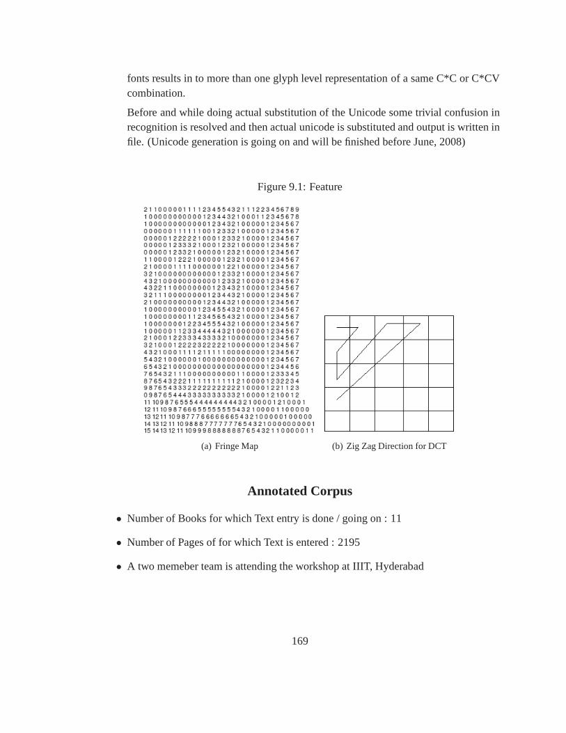
fonts results in to more than one glyph level representationof a same C*C or C*CVcombination.
Before and while doing actual substitution of the Unicode some trivial confusion inrecognition is resolved and then actual unicode is substituted and output is written infile. (Unicode generation is going on and will be finished before June, 2008)
Figure 9.1: Feature
(a) Fringe Map (b) Zig Zag Direction for DCT
Annotated Corpus
• Number of Books for which Text entry is done / going on : 11
• Number of Pages of for which Text is entered : 2195
• A two memeber team is attending the workshop at IIIT, Hyderabad
169

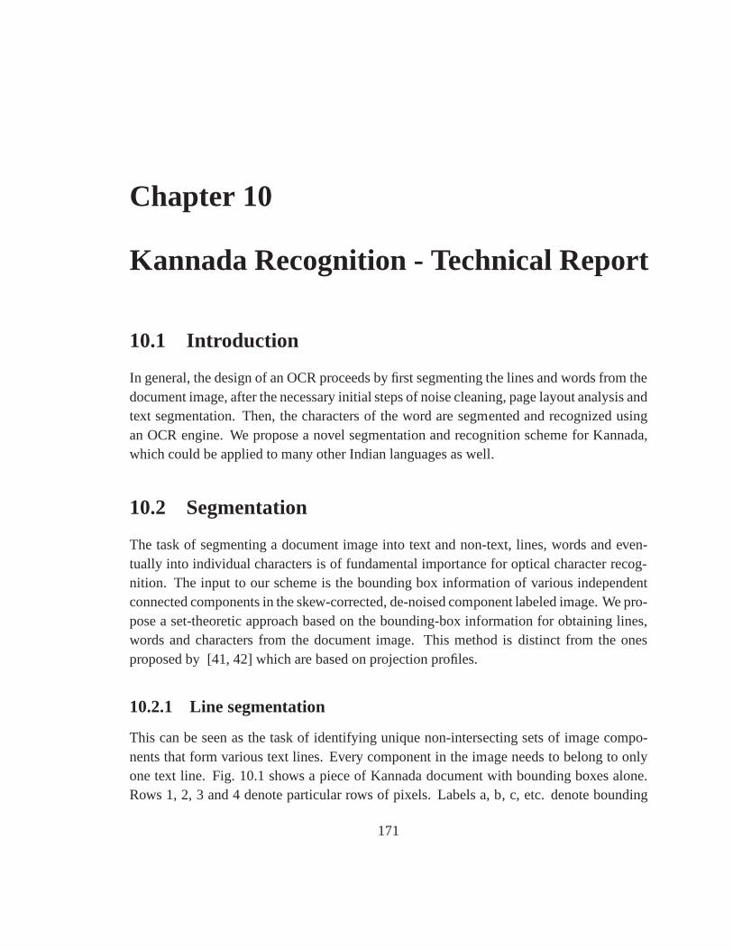
Chapter 10
Kannada Recognition - Technical Report
10.1 Introduction
In general, the design of an OCR proceeds by first segmenting the lines and words from thedocument image, after the necessary initial steps of noise cleaning, page layout analysis andtext segmentation. Then, the characters of the word are segmented and recognized usingan OCR engine. We propose a novel segmentation and recognition scheme for Kannada,which could be applied to many other Indian languages as well.
10.2 Segmentation
The task of segmenting a document image into text and non-text, lines, words and even-tually into individual characters is of fundamental importance for optical character recog-nition. The input to our scheme is the bounding box information of various independentconnected components in the skew-corrected, de-noised component labeled image. We pro-pose a set-theoretic approach based on the bounding-box information for obtaining lines,words and characters from the document image. This method isdistinct from the onesproposed by [41, 42] which are based on projection profiles.
10.2.1 Line segmentation
This can be seen as the task of identifying unique non-intersecting sets of image compo-nents that form various text lines. Every component in the image needs to belong to onlyone text line. Fig. 10.1 shows a piece of Kannada document with bounding boxes alone.Rows 1, 2, 3 and 4 denote particular rows of pixels. Labels a, b, c, etc. denote bounding
171
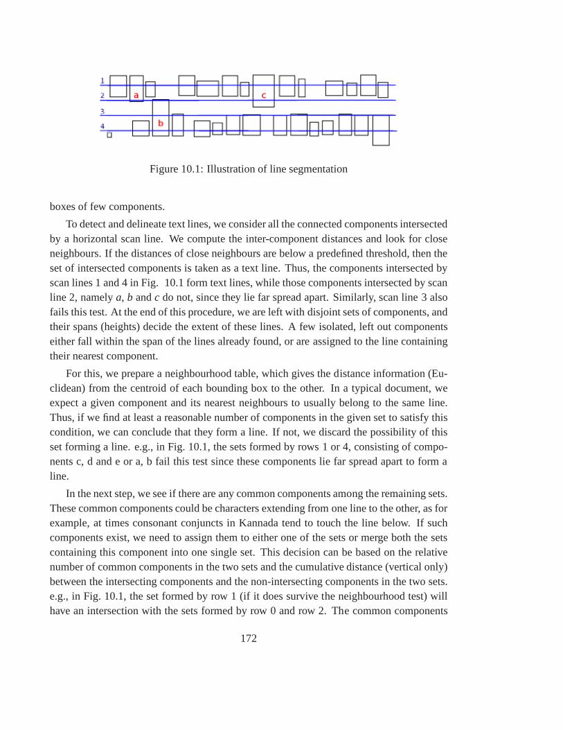
Figure 10.1: Illustration of line segmentation
boxes of few components.
To detect and delineate text lines, we consider all the connected components intersectedby a horizontal scan line. We compute the inter-component distances and look for closeneighbours. If the distances of close neighbours are below apredefined threshold, then theset of intersected components is taken as a text line. Thus, the components intersected byscan lines 1 and 4 in Fig. 10.1 form text lines, while those components intersected by scanline 2, namelya, b andc do not, since they lie far spread apart. Similarly, scan line3 alsofails this test. At the end of this procedure, we are left withdisjoint sets of components, andtheir spans (heights) decide the extent of these lines. A fewisolated, left out componentseither fall within the span of the lines already found, or areassigned to the line containingtheir nearest component.
For this, we prepare a neighbourhood table, which gives the distance information (Eu-clidean) from the centroid of each bounding box to the other.In a typical document, weexpect a given component and its nearest neighbours to usually belong to the same line.Thus, if we find at least a reasonable number of components in the given set to satisfy thiscondition, we can conclude that they form a line. If not, we discard the possibility of thisset forming a line. e.g., in Fig. 10.1, the sets formed by rows1 or 4, consisting of compo-nents c, d and e or a, b fail this test since these components lie far spread apart to form aline.
In the next step, we see if there are any common components among the remaining sets.These common components could be characters extending fromone line to the other, as forexample, at times consonant conjuncts in Kannada tend to touch the line below. If suchcomponents exist, we need to assign them to either one of the sets or merge both the setscontaining this component into one single set. This decision can be based on the relativenumber of common components in the two sets and the cumulative distance (vertical only)between the intersecting components and the non-intersecting components in the two sets.e.g., in Fig. 10.1, the set formed by row 1 (if it does survive the neighbourhood test) willhave an intersection with the sets formed by row 0 and row 2. The common components
172
being d and e in the former case and c in the latter. So, c, d and eform a weak linkwith line information presented by row 0 and row 3. However, the no. of intersectingcomponents is too low (2 and 1 respectively). Based on this number, and the relativedistances between these components, we can declare the linkto be spurious. However, theability to discriminate weak links is dependent on a few thresholds, which must be carefullychosen.
Finally, we will be left with disjoint sets of components, and we decide that their spans(heights) decide the extent of these lines.
However, a few components can be left out from all the lines when we discard setsbased on distance constraints on components. At this stage,they may either naturally fallwithin the span of the lines we found, or can be assigned to oneof the lines based on thedistances to the lines, or to the line on which the first few nearest neighbours belong. In caseof very distant and isolated components, one may even chooseto discard the componentfor the purpose of recognition, since they could be spuriouselements or may contain littleinformation.e.g., in Fig. 10.1, if row 4 contains only components a and b, based on theneighbourhood criterion, the seta, b would be discarded as a line. However, thanks to theset formed by row 3, b would eventually get a line label. However, component a would beleft without a line label at the end of this procedure. However, still, component a may liewithin the columns spanned by the components formed by row 3 and hence associated withthe same line. Or, we could choose to assign it to the line to which its nearest neighbourbelongs, or based on the distance to its nearest neighbour, and with some global statisticsabout nearest neighbour distances, it could even be denied aline label and hence furtherrecognition.
For the algorithms we developed, we put a constraint that, for a set of components toform a line, at least a third of them should have their nearestneighbours within the set. Weassociated weak-links and un-assigned components to various lines based on the distancesto few nearest neighbours.
10.2.2 Word and character segmentation
Following line segmentation, one may obtain information ofcolumns which do not passthrough any bounding box on a given line. We accumulate the spacing information soobtained from all the lines of the document and then binarizethe distances to obtain wordand character separation information.
However, we propose an alternative weighted distance spacing measurement whichmay give better results in case of documents containing multiple font sizes. One can visu-alize the fact that, usually, if the font size increases, so do the word and character spacing.
173
So, if the spacing between two components is weighted as a function of the sizes of thecomponents across the gap (by average of heights), one may obtain a more meaningful in-formation about the spacing. This can very effectively be done by using the bounding boxinformation we used for line segmentation, and hence turns out to be an additional benefitof using this approach.
10.2.3 Akshara demarcation
Following line segmentation, it would be logical to pursue word segmentation. However,due to the nature of certain scripts, there may be a need to demarcate Aksharas, which cancontain two or more components. In Kannada script, aksharascontain components whichare stacked vertically, at times with some horizontal offset. Though, grammatically, twohorizontally non-overlapping components can still form one single akshara, for the purposeof recognition, it is prudent to treat them as separate entities. In some sense, it is moreeasier to recognize components (can be looked at as glyph) than whole aksharas. So, forthe present discussion, we treat those components that do not have overlapping columnsas separate aksharas. But the more interesting question is,does an overlap between twocomponents always mean that they belong to the same akshara?
It turns out that, that may not be the case in Kannada script. When multiple consonantconjuncts appear in writing/print, it is commonly found that the following consonant orvowel can have overlapping columns with some consonant conjuncts. Hence, we need toadopt some strategy to demarcate aksharas. In the algorithms we have developed and tested,if the centroid of one component falls within the horizontalspan of any other component,we declare that the components belong to the same akshara. This may leave out a fewconsonant conjuncts or vowel appendages from being associated to the akshara in the rightmanner. We handle this in post-processing.
10.3 Character classification
The problem of recognizing printed Kannada characters has been studied in [42, 41]. Aswe find, it is one of being able to distinguish data from a largenumber of classes, typi-cally around 450. This we find is the case with many Indian scripts [43]. The problem ofclassifying data from a large number of classes has been studied in [44]. The study showsthat there will be a tremendous increase in computational costs with increase in number ofclasses. Hence, most attempted solutions try to reduce the classes one needs to distinguish,by breaking the characters into smaller, repetitive subunits, usually by some script depen-dent segmentation technique [42, 41]. Each subunit is individually recognized, and finally,
174
a conclusion is drawn about the character based on the recognized subunits. In general,most OCR’s for Indian scripts adopt this strategy [43]. However, the rules for segmentingthe characters are usually script specific, and entail many assumptions. This makes it hardto adapt any such technique to new scripts. In what follows, we report a novel and effectivestrategy to solve this problem and discuss about its merits and limitations.
The strategy is based on the fundamental observation that, among the set of charactersthat make up a script, any two visually distinct characters are bound to differ either in thenumber of strokes they are composed of, or in the nature of interconnections among thestrokes. In this study, we cast this inherent property that distinguishes any two charactersinto graph theoretic framework by associating the skeletonized form of each character witha planar graph. The strokes are mapped to edges of a graph, andthe stroke junctions aremapped to vertices. The character can thus be identified by the incidence matrix of theassociated graph. During recognition, a character component is classified by either a lookup into a table built by the above methodology using trainingsamples and if this does notgive a unique class label, it is followed by classification based on some image features.This strategy is invariant to character height and fairly robust to font variations. Here, weintroduce the terminology used in the rest of the article.
Graph - A set of non-empty points called vertices, and a set of edgesthat link the vertices
Signed graph - A graph in which each end of an edge has a positive or negativesign
Weighted Graph - A graph with weights associated with each edge
Planar Graph - A graph that can be drawn on a plane
Adjacent edges- Two distinct edges are said be adjacent if they have at leastone vertexin common
Adjacent vertices - Two distinct vertices are said be adjacent if there are one or moreedges connecting them
Degree of a vertex - The number of distinct edges that are incident to it
Loop - An edge that links a vertex to itself
Terminal vertex - A vertex of degree one (an end point)
The idea of adjacency and incidence have been represented byincidence matrix. Sup-poseG is a graph with a vertex setV (G) = {v1, . . . , vn} and an edge setE(G) =
175

{e1, . . . , em}. We denotevj ∼ ek if and only if thejth vertex ofV is incident with thekth edge ofE. Then then×m incidence matrixI, whosejkth entry isIjk, is defined by:
Ijk = 1 iff vj ∼ ek; 0 else (10.1)
The following example serves to illustrate the above idea. Fig. 10.2 shows a simplegraph. {a, b, c & d} denotes the set of vertices and{1, 2, 3, 4, 5, 6} is the edge set. Wefollow the convention that edges entering a vertex give positive sign to the vertex and edgesleaving a vertex give a negative sign to the vertex in the incidence matrix. Vertices{a, b}are of degree3 andb is of degree4. Vertexd is a terminal vertex. The incidence matrix forthe graph is given by the center part of the table in Fig. 10.2.The last two columns indicatethe kind of edges (normal or loop). The penultimate column isthe sum of the correspondingrow entries of the incidence matrix and the last column is thesum of the absolute values ofthe corresponding row entries. Similarly, the last row indicates the degree of the verticesand is the sum of the absolute values in the columns. The penultimate row is the summationof the corresponding columns of the incidence matrix. Note the fact that edge6 is a loopis clearly shown by the entry1 in the last two columns of the table. Note that the fact thatvertexd is a terminal vertex is clearly evident from the last row. Assigning directions tothe loops is a matter of convention and could be based on the position of the vertex withrespect to the loop.
a b c d1 1 0 -1 0 0 22 1 0 -1 0 0 23 -1 1 0 0 0 24 0 1 -1 0 0 25 0 -1 0 1 0 26 0 0 1 0 1 1
1 1 -2 13 3 4 1
Figure 10.2: A graph and its signed incidence matrix
10.4 Graph based Representation for components
The use of skeletonized or infinitely thinned versions of character components in classifi-cation tasks is an established practice, since it renders the classification task robust to font
176
thickness and style variations. In the proposed technique,in addition to this advantage, weuse them to obtain information about junctions and strokes in the character.
Once the edges and vertices are obtained, we can interpret the component as a planargraph. If we adopt a systematic way to assign directions to edges, we could associate asigned incidence matrix with the component. e.g., depending on whether the edge verticesare separated more by height/width, we could assign positive values to up/left vertices andnegative values to down/right vertices. Since this too can give rise to ambiguity in casethe height and width differences between two vertices are the same, we could arbitrarilygive more importance to height than to width or the other way round. Essentially, weshould have a methodical way of assigning directions to edges. Now, if we have a way todistinguish the various edges that make up the component, wecan associate a label (weight)to each edge, and thus associate a weighted signed incidencematrix with the component.The edge weights can be obtained as predictions from a classifier trained to distinguishvarious edge types that can occur in the script.
As we can observe, we can expect character components belonging to different classesto have different or same incidence matrices. Not only that,visually similar looking com-ponents could end up having very different matrix representations. Also, due to font vari-ations, we can expect the same component class to have multiple graph representations.This segregation leads to four important categories of character components.
Object kind 1 - A point
Object kind 2 - Closed loops (no vertices)
Object kind 3 - Simple edges joining two terminal vertices
Object kind 4 - Objects with more than one edges/vertices
Given that we have a mechanism to get edges and vertices and perhaps even the edgelabels, obtaining the incidence matrix would have been a simple task, if we could order theedges and vertices of a given component in a manner that wouldremain invariant undernormal font variations. However, since vectors do not have anatural ordering, any spatialordering scheme can produce a different incidence matrix for very small changes in positionof vertices or edges. To circumvent this problem, we can firstorder the edges based on theirrelative energies. However, the vertices do not have such anattribute. So, we resort to thenotion of “vertex significance”, wherein we consider the sumof the energies of the edgesincident at a vertex as an attribute to rank the vertices. i.e, vertices at which longer andor more numerous edges converge will have higher ranking than the vertices with few andor shorter edges. An incident matrix with edges and verticesordered in this manner can
177
yield a robust representation for the character, since the ordering of relative edge strengthsof a component remains fairly stable under normal font variations. However, in cases ofties in ranking, we arbitrarily assign ranks to the competing entities. However, we restrictour study to the case where we do not use edge labels, i.e., we do not do the task of edgeclassification. We later re-visit the case where we considerthe probable uses of edge labels.
10.5 Similarity of the Components
Graph matching has been a subject of study for many years now [45, 46]. In this work,we report a simple, yet useful strategy for comparing graphs. We resort to a few discrete,qualitative notion of distance, instead of a quantitative one.
Let I be the signed incidence matrix. In this state, the rows ofI are ordered in thedescending order of relative edge strengths. The columns ofI would be stored in therank of “verticex significance” we described earlier. Though this may not give a uniquerepresentation to the graph (since many vertices can have same significance and manyedges many have same strength), it seems to be a fairly robustrepresentation, as evidencedby the results.
We collect the information we have from the graph in four separate row vectors whichwe callRi, i = 1 . . . 4. We define the row vectors as follows -
• R1 = [no. of edges no. of vertices]
• R2 = [euler no. no. of non zero elements in I]
• R3 = [vertical projection of abs(I) horizontal projection of abs(I)]
• R4 = [vertical projection of I horizontal projection of I]
R1 andR2 contain information about gross features of the incidence matrix. R3 contains theinformation from unsigned incidence matrixabs(I) (abs(I) contains the absolute values ofthe entries ofI). Although, to get the whole information ofI, we need to put down all itsindividual elements, we resort to using just this, since it simplifies the task of representation.Similarly,R4 contains partial information from the signed incidence matrix in a condensedform.
Given the representationsRpi andRq
j ; i, j = 1 . . . 4, for two character samples num-beredp andq, we define the similarity between them as follows-
• if Rpi = Rq
i for i = 1 . . . 4, then they are said to produce anexact or (M4) match
178

• if Rpi = Rq
i for i = 1, 2, 3 and not for n = 4, then they are said to match only upto incidence or (M3)
• if Rpi = Rq
i for i = 1, 2 and not for n = 3, 4, then they are said to match only upto non-zero elements or (M2)
• if Rpi = Rq
i for i = 1 and not for n = 2, 3, 4, then they are said to match only upto cardinality or (M1)
• if Rpi 6= Rq
i for i = 1, then, they are said to beunrelated
Now, based on these distances we have defined, we try to qualify the kinds of relation-ships the classes may develop, based on the graph representations of the training samples.Let the training samples belong to classesCk, k = 1, 2 . . .. Let Ra,m
i , m = 1 . . . , p andRb,n
i , n = 1 . . . , q, i = 1 . . . 4 be the representations of training samples (p andq in num-bers) associated with classesCa andCb, respectively.
• if for some samplesr ands, if Ra,ri = Rb,s
i , ∀i, anda 6= b, then,Ca andCb are saidto be inconflict at level 4
• if for some samplesr ands, if Ra,ri = Rb,s
i , i = 1, 2, 3 and not i = 4, anda 6= b,thenCa andCb are said to be inconflict at level 3
• Similarly, we can defineconflicts at level 2 and 1
• Classes in conflict are said to berelated
• if for no samplesr and s, if Ra,r1 = Rb,s
1 , then classesCa andCb are said to beunrelated or isolated
• for some samplesr ands, if Ra,ri = Ra,s
i , i = 1 . . . j and Ra,rj+1 6= Ra,s
j+1 or j = 4,thenr ands are said to beequivalent representations of classCa up to levelj
Equipped with these qualitative distance measures betweenpatterns and classes, weproceed to explore the possible classification strategies we can adopt.
10.6 The Classification strategy
The graph based technique effectively divides the classification task into smaller sub-tasks,provided that we get enough information about the nature of relationships between theclasses from the training samples. Then, the problem can be conquered by dividing the
179
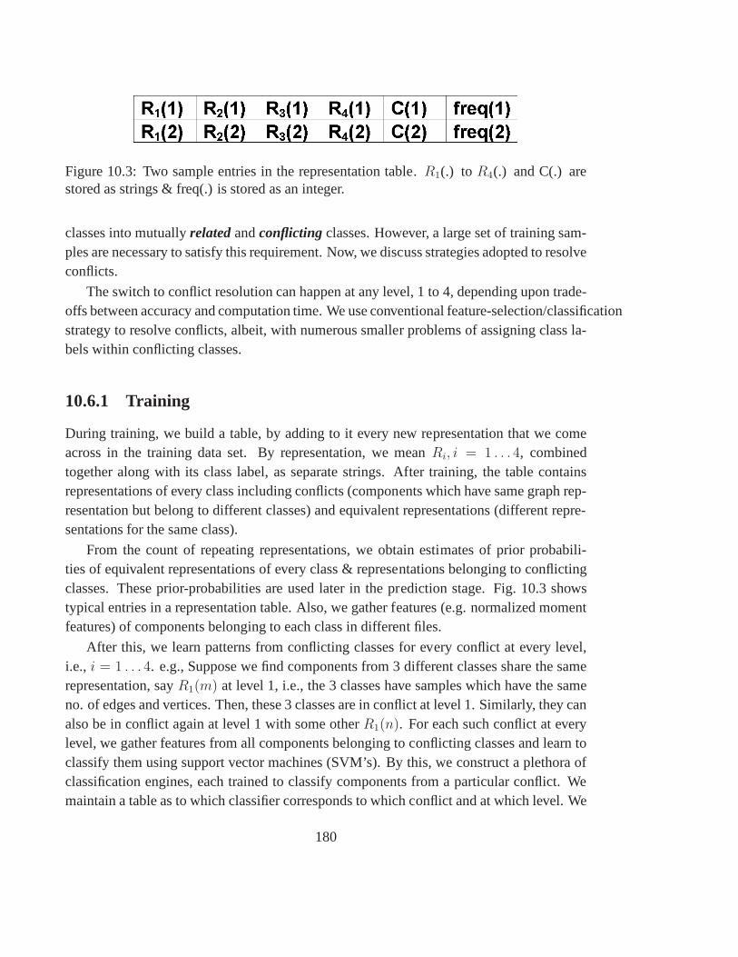
Figure 10.3: Two sample entries in the representation table. R1(.) to R4(.) and C(.) arestored as strings & freq(.) is stored as an integer.
classes into mutuallyrelatedandconflicting classes. However, a large set of training sam-ples are necessary to satisfy this requirement. Now, we discuss strategies adopted to resolveconflicts.
The switch to conflict resolution can happen at any level, 1 to4, depending upon trade-offs between accuracy and computation time. We use conventional feature-selection/classificationstrategy to resolve conflicts, albeit, with numerous smaller problems of assigning class la-bels within conflicting classes.
10.6.1 Training
During training, we build a table, by adding to it every new representation that we comeacross in the training data set. By representation, we meanRi, i = 1 . . . 4, combinedtogether along with its class label, as separate strings. After training, the table containsrepresentations of every class including conflicts (components which have same graph rep-resentation but belong to different classes) and equivalent representations (different repre-sentations for the same class).
From the count of repeating representations, we obtain estimates of prior probabili-ties of equivalent representations of every class & representations belonging to conflictingclasses. These prior-probabilities are used later in the prediction stage. Fig. 10.3 showstypical entries in a representation table. Also, we gather features (e.g. normalized momentfeatures) of components belonging to each class in different files.
After this, we learn patterns from conflicting classes for every conflict at every level,i.e., i = 1 . . . 4. e.g., Suppose we find components from 3 different classes share the samerepresentation, sayR1(m) at level 1, i.e., the 3 classes have samples which have the sameno. of edges and vertices. Then, these 3 classes are in conflict at level 1. Similarly, they canalso be in conflict again at level 1 with some otherR1(n). For each such conflict at everylevel, we gather features from all components belonging to conflicting classes and learn toclassify them using support vector machines (SVM’s). By this, we construct a plethora ofclassification engines, each trained to classify components from a particular conflict. Wemaintain a table as to which classifier corresponds to which conflict and at which level. We
180
call this as classifier pointer table.
10.6.2 Prediction
Fig. 10.4 shows a schematic of the classification strategy. Given a test pattern, we obtain itsrepresentation in the representation table from its graph &see whether such a representationexists by a simple string comparison. If there is a match, andif only one class has theparticular representation (no conflicts), then we assign the test pattern to the correspondingclass.
However, if multiple classes share the same representation(conflicts), we use the clas-sifier specifically trained with samples from conflicting classes at the highest level of rep-resentation, to classify the pattern. e.g., given a test pattern, if it so happens that we donot find a match forR4 of the test pattern in the representation table, but find thatconflictsexist at level 3, then it is obvious that conflicts exist at level 2 and level 1 also. This is dueto the very nature by which the representation table is generated. Though we can choose aclassifier trained to resolve conflicts at any of the levels 1,2 or 3, we choose the classifiertrained to resolve conflicts at level 3, instead of the ones trained to resolve conflicts at level2 and 1. i.e., we try to narrow down the conflicts as much as possible using the graphbased representation. This, as we show later reduces the computational complexity to agreat extent, as compared to trying to resolve conflicts at lower levels. The reason being,as we go higher levels of representations, the probable number of classes sharing the samerepresentation will go down. So, a classifier trained to resolve conflicts at higher levelswill have to be trained with data from fewer classes. This means that the classifier willrequire less computation resources. While resolving conflicts, we can also use the priorprobability information obtained in the training phase if we can get probabilistic outputsfrom the classifier instead of class labels. The probabilistic outputs from the classifier canbe weighed by the prior probabilities of a pattern belongingto a particular class to make afinal decision.
When we do not find any match based even at level 1, (i.e., the sample is unrelated toany training data), we can declare that the test pattern doesnot belong to any of the givenclasses.
10.6.3 Spline Features
In addition to the features based on graph representation, spline features are also evalu-ated. Centralize the character in the image The data of the image, which is a matrix (saydimension is rows X columns) is converted to a square image byzero padding the original
181

Figure 10.4: The classification strategy
182
matrix. If rows ¿ columns, then (rows columns) more columns are added to the image else(columns rows) more rows are added to the image data to get thenew dimension rows1 Xcols1. This image is then zero padded both along the rows and columns by an amount ofmax (rows, columns) * 0.1. To handle the cases, where the image is very small, the condi-tion (rows1 ¡ splines order + splines pieces) is checked. If this condition is satisfied, thenzero padding is done along the rows and columns by an amount (splines order + splinespieces rows )/ 2. The zero padding is done in order to preservethe corners and the changeswhich occur along the bounding boxes.
Knot Vector Calculation The interval (1 to rows) and (1 to columns) is divided intoequal parts and stored in matrices Knots1 and Knots2. The matrices are normalized to havevalues in the interval [0 1] by dividing Knots1 and Knots2 by max(rows,columns).
Input The C Code Works by specifying the image data, spline order and spline piecesas input. The C code takes only one connected component in theimage. The C code wastested with Kannada database of characters having 50 X 50 size consonant, 30 X 30 vottusand Indian numbers and some special characters such as , ? , / ,etc. The C code works finewith image size ¿ 80 pixels. However, for some special symbols, such as, . etc. where theimage size goes below 80 pixels, it fails in these characters. We need to use a spline ordergreater than 2 and give only .bmp images.
Output The output of the program is a matrix, which depends onthe inputs: No. ofspline pieces and order of the splines. Typically, for orderof splines = 4 and No. of splinepieces = 10, coefficient matrix is of size 11 X 11 and for splines order = 4 and splines pieces= 8, the coefficient matrix is of size 9 X 9 .
10.7 Experiments, Results and Discussions
10.7.1 Data Set
The data set contained computer generated character components, digits and punctuationfrom 21 different fonts (various Nudi, Baraha and Kuvempu Kannada fonts and a fewsimple decorative fonts). The font size varied from 50 to 100in steps of10 and the char-acters were printed with100 dpi resolution. We found446 independent components in thewhole script (including very basic punctuation and rarely used characters). We had33, 552
samples in all, providing, on an average, about75 samples for all possible components ofKannada script. Besides, the font size variation mimics theusual size of components indocuments scanned at 300dpi. Since we did not have a real dataset with good font and fontsize variation or as many no. of classes as required, we decided to use this data set.
183
10.7.2 Pre-processing
In Kannada, very small edges connected to terminal verticesserve little purpose in iden-tifying characters. So, we choose to retain only the significant terminal edges. Similarly,small edges connecting non-terminal vertices are coalesced with the incident vertices toform a single vertex. These processing steps make graph representations more robust tofont variations.
Characters may have holes in edge strokes as as a result of noise and binarization. Thin-ning is sensitive to presence of holes, and if not filled, theycan lead to unwanted thinnedcharacters, and thereby to wrong graphs. This is the biggestchallenge to graph based rep-resentations of characters. Though removing small edges may alleviate the situation, agood morphological pre-processing step can mitigate the problem to a great extent. Weused morphological majority operation, followed by spurring, to overcome these noise ef-fects. However, more sophisticated morphological operations may be needed to handlenoisy data.
10.7.3 Feature extraction
We choose features that do not require image scaling, namelynormalized central momentsand 2d-spline features. Though moment features have been elaborately studied, the use of2d-splines for this purpose has received little attention in the Indian OCR community. The2d-least squares splines can be used for feature extractionwithout scaling. Since the fea-tures are solutions to sets of linear equations these are notcomputationally very expensive.As we seen later, they tend to learn the samples relatively well compared to normalizedcentral moments and hence seem to be better suited for the task on hand. Though compar-isons can be made across various features to choose the best feature for the task on hand,the focus of the paper being not feature selection, we have limited our features to thesetwo varieties. However, limited comparative studies seem to show that 2d-splines can bevery good contenders as features for OCR data. Fig. 10.5 and Fig. 10.6 show the 5-foldcross validation results obtained from libsvm [?] using an RBF kernel with 25 normalizedcentral moment and 25 2d-spline features respectively, on objects of kind 4. The superiorperformance of 2d-spline features evidenced by the broadercontours at all accuracy levelsand at lowerγ values is clear from these plots.
10.7.4 Experiments and discussions
We segregated the data set into various kinds of objects, as discussed in section 10.4. Westudied the distribution of various character classes in each of the object kind. When this
184
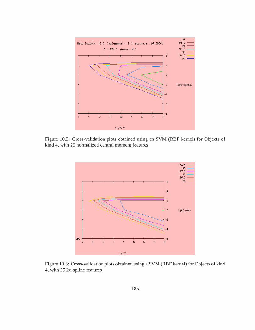
Figure 10.5: Cross-validation plots obtained using an SVM (RBF kernel) for Objects ofkind 4, with 25 normalized central moment features
Figure 10.6: Cross-validation plots obtained using a SVM (RBF kernel) for Objects of kind4, with 25 2d-spline features
185
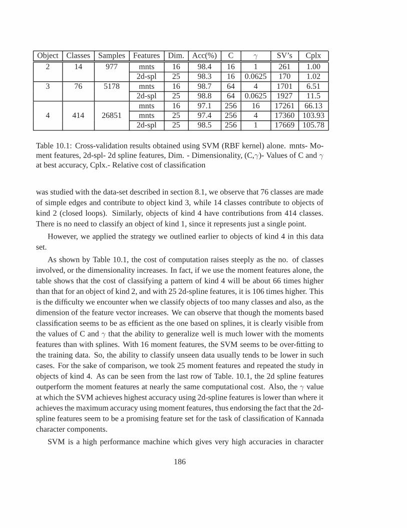
Object Classes Samples Features Dim. Acc(%) C γ SV’s Cplx
2 14 977 mnts 16 98.4 16 1 261 1.002d-spl 25 98.3 16 0.0625 170 1.02
3 76 5178 mnts 16 98.7 64 4 1701 6.512d-spl 25 98.8 64 0.0625 1927 11.5mnts 16 97.1 256 16 17261 66.13
4 414 26851 mnts 25 97.4 256 4 17360 103.932d-spl 25 98.5 256 1 17669 105.78
Table 10.1: Cross-validation results obtained using SVM (RBF kernel) alone. mnts- Mo-ment features, 2d-spl- 2d spline features, Dim. - Dimensionality, (C,γ)- Values of C andγat best accuracy, Cplx.- Relative cost of classification
was studied with the data-set described in section 8.1, we observe that 76 classes are madeof simple edges and contribute to object kind 3, while 14 classes contribute to objects ofkind 2 (closed loops). Similarly, objects of kind 4 have contributions from 414 classes.There is no need to classify an object of kind 1, since it represents just a single point.
However, we applied the strategy we outlined earlier to objects of kind 4 in this dataset.
As shown by Table 10.1, the cost of computation raises steeply as the no. of classesinvolved, or the dimensionality increases. In fact, if we use the moment features alone, thetable shows that the cost of classifying a pattern of kind 4 will be about 66 times higherthan that for an object of kind 2, and with 25 2d-spline features, it is 106 times higher. Thisis the difficulty we encounter when we classify objects of toomany classes and also, as thedimension of the feature vector increases. We can observe that though the moments basedclassification seems to be as efficient as the one based on splines, it is clearly visible fromthe values of C andγ that the ability to generalize well is much lower with the momentsfeatures than with splines. With 16 moment features, the SVMseems to be over-fitting tothe training data. So, the ability to classify unseen data usually tends to be lower in suchcases. For the sake of comparison, we took 25 moment featuresand repeated the study inobjects of kind 4. As can be seen from the last row of Table. 10.1, the 2d spline featuresoutperform the moment features at nearly the same computational cost. Also, theγ valueat which the SVM achieves highest accuracy using 2d-spline features is lower than where itachieves the maximum accuracy using moment features, thus endorsing the fact that the 2d-spline features seem to be a promising feature set for the task of classification of Kannadacharacter components.
SVM is a high performance machine which gives very high accuracies in character
186
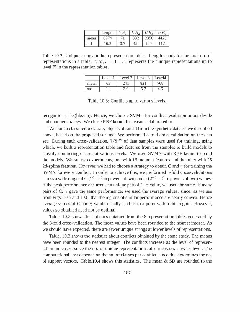
Length UR1 UR2 UR3 UR4
mean 6274 71 332 2356 4425std 16.2 0.7 4.9 9.9 11.1
Table 10.2: Unique strings in the representation tables. Length stands for the total no. ofrepresentations in a table.URi, i = 1 . . . 4 represents the “unique representations up tolevel i” in the representation tables.
Level 1 Level 2 Level 3 Level4mean 63 241 821 708std 1.1 3.0 5.7 4.6
Table 10.3: Conflicts up to various levels.
recognition tasks(libsvm). Hence, we choose SVM’s for conflict resolution in our divideand conquer strategy. We chose RBF kernel for reasons elaborated in.
We built a classifier to classify objects of kind 4 from the synthetic data set we describedabove, based on the proposed scheme. We performed 8-fold cross-validation on the dataset. During each cross-validation,7/8 th of data samples were used for training, usingwhich, we built a representation table and features from thesamples to build models toclassify conflicting classes at various levels. We used SVM’s with RBF kernel to buildthe models. We ran two experiments, one with 16 moment features and the other with 252d-spline features. However, we had to choose a strategy to obtain C andγ for training theSVM’s for every conflict. In order to achieve this, we performed 3-fold cross-validationsacross a wide range of C (20−26 in powers of two) andγ (2−8−22 in powers of two) values.If the peak performance occurred at a unique pair of C,γ value, we used the same. If manypairs of C,γ gave the same performance, we used the average values, since, as we seefrom Figs. 10.5 and 10.6, that the regions of similar performance are nearly convex. Henceaverage values of C andγ would usually lead us to a point within this region. However,values so obtained need not be optimal.
Table 10.2 shows the statistics obtained from the 8 representation tables generated bythe 8-fold cross-validation. The mean values have been rounded to the nearest integer. Aswe should have expected, there are fewer unique strings at lower levels of representations.
Table. 10.3 shows the statistics about conflicts obtained bythe same study. The meanshave been rounded to the nearest integer. The conflicts increase as the level of represen-tation increases, since the no. of unique representations also increases at every level. Thecomputational cost depends on the no. of classes per conflict, since this determines the no.of support vectors. Table.10.4 shows this statistics. The mean & SD are rounded to the
187
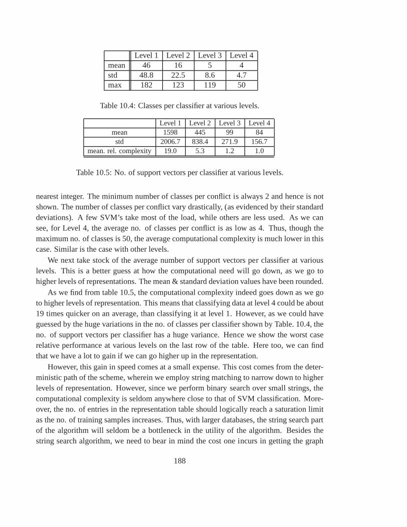
Level 1 Level 2 Level 3 Level 4mean 46 16 5 4std 48.8 22.5 8.6 4.7max 182 123 119 50
Table 10.4: Classes per classifier at various levels.
Level 1 Level 2 Level 3 Level 4mean 1598 445 99 84std 2006.7 838.4 271.9 156.7
mean. rel. complexity 19.0 5.3 1.2 1.0
Table 10.5: No. of support vectors per classifier at various levels.
nearest integer. The minimum number of classes per conflict is always 2 and hence is notshown. The number of classes per conflict vary drastically, (as evidenced by their standarddeviations). A few SVM’s take most of the load, while others are less used. As we cansee, for Level 4, the average no. of classes per conflict is as low as 4. Thus, though themaximum no. of classes is 50, the average computational complexity is much lower in thiscase. Similar is the case with other levels.
We next take stock of the average number of support vectors per classifier at variouslevels. This is a better guess at how the computational need will go down, as we go tohigher levels of representations. The mean & standard deviation values have been rounded.
As we find from table 10.5, the computational complexity indeed goes down as we goto higher levels of representation. This means that classifying data at level 4 could be about19 times quicker on an average, than classifying it at level 1. However, as we could haveguessed by the huge variations in the no. of classes per classifier shown by Table. 10.4, theno. of support vectors per classifier has a huge variance. Hence we show the worst caserelative performance at various levels on the last row of thetable. Here too, we can findthat we have a lot to gain if we can go higher up in the representation.
However, this gain in speed comes at a small expense. This cost comes from the deter-ministic path of the scheme, wherein we employ string matching to narrow down to higherlevels of representation. However, since we perform binarysearch over small strings, thecomputational complexity is seldom anywhere close to that of SVM classification. More-over, the no. of entries in the representation table should logically reach a saturation limitas the no. of training samples increases. Thus, with larger databases, the string search partof the algorithm will seldom be a bottleneck in the utility ofthe algorithm. Besides thestring search algorithm, we need to bear in mind the cost one incurs in getting the graph
188
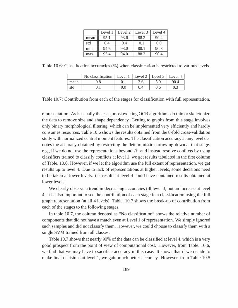
Level 1 Level 2 Level 3 Level 4mean 95.1 93.6 88.2 90.4std 0.4 0.4 0.1 0.0min 94.6 93.0 88.1 90.3max 95.4 94.0 88.3 90.4
Table 10.6: Classification accuracies (%) when classification is restricted to various levels.
No classification Level 1 Level 2 Level 3 Level 4mean 0.8 0.1 3.6 5.0 90.4std 0.1 0.0 0.4 0.6 0.3
Table 10.7: Contribution from each of the stages for classification with full representation.
representation. As is usually the case, most existing OCR algorithms do thin or skeletonizethe data to remove size and shape dependency. Getting to graphs from this stage involvesonly binary morphological filtering, which can be implemented very efficiently and hardlyconsumes resources. Table 10.6 shows the results obtained from the 8-fold cross-validationstudy with normalized central moment features. The classification accuracy at any level de-notes the accuracy obtained by restricting the deterministic narrowing-down at that stage.e.g., if we do not use the representations beyondR1 and instead resolve conflicts by usingclassifiers trained to classify conflicts at level 1, we get results tabulated in the first columnof Table. 10.6. However, if we let the algorithm use the full extent of representation, we getresults up to level 4. Due to lack of representations at higher levels, some decisions needto be taken at lower levels. i.e, results at level 4 could havecontained results obtained atlower levels.
We clearly observe a trend in decreasing accuracies till level 3, but an increase at level4. It is also important to see the contribution of each stage in a classification using the fullgraph representation (at all 4 levels). Table. 10.7 shows the break-up of contribution fromeach of the stages to the following stages.
In table 10.7, the column denoted as “No classification” shows the relative number ofcomponents that did not have a match even at Level 1 of representation. We simply ignoredsuch samples and did not classify them. However, we could choose to classify them with asingle SVM trained from all classes.
Table 10.7 shows that nearly90% of the data can be classified at level 4, which is a verygood prospect from the point of view of computational cost. However, from Table. 10.6,we find that we may have to sacrifice accuracy in this case. It shows that if we decide tomake final decisions at level 1, we gain much better accuracy.However, from Table 10.5
189
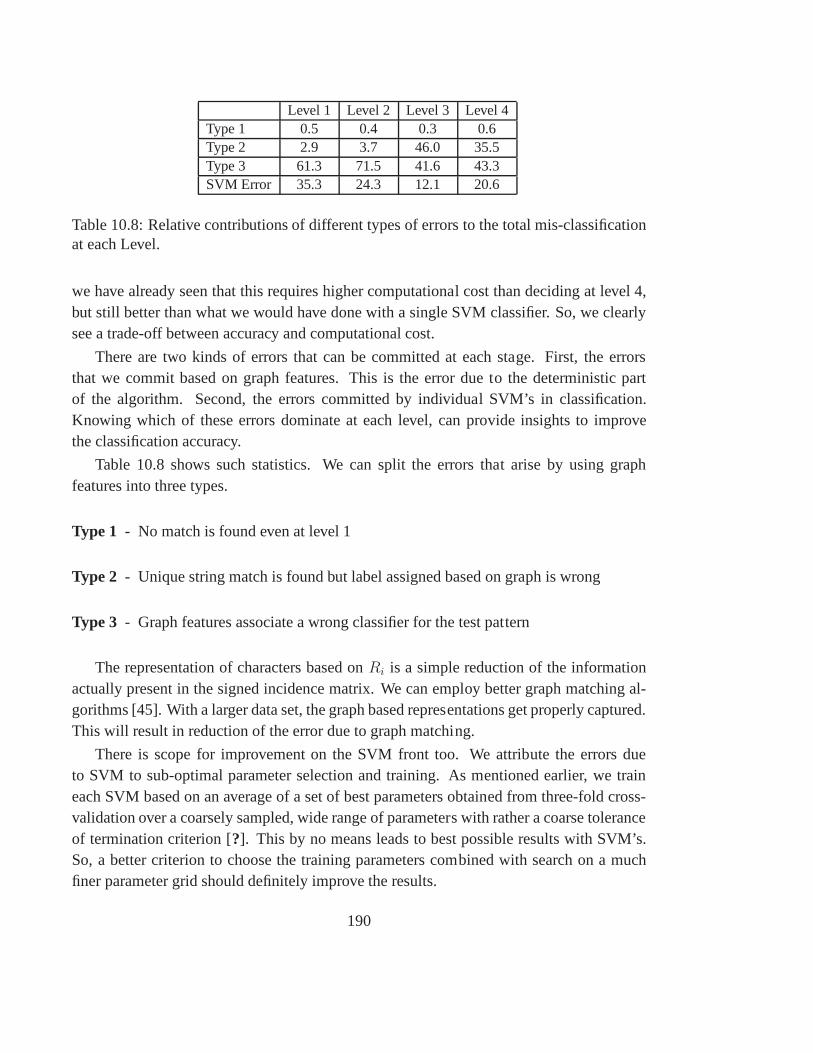
Level 1 Level 2 Level 3 Level 4Type 1 0.5 0.4 0.3 0.6Type 2 2.9 3.7 46.0 35.5Type 3 61.3 71.5 41.6 43.3SVM Error 35.3 24.3 12.1 20.6
Table 10.8: Relative contributions of different types of errors to the total mis-classificationat each Level.
we have already seen that this requires higher computational cost than deciding at level 4,but still better than what we would have done with a single SVMclassifier. So, we clearlysee a trade-off between accuracy and computational cost.
There are two kinds of errors that can be committed at each stage. First, the errorsthat we commit based on graph features. This is the error due to the deterministic partof the algorithm. Second, the errors committed by individual SVM’s in classification.Knowing which of these errors dominate at each level, can provide insights to improvethe classification accuracy.
Table 10.8 shows such statistics. We can split the errors that arise by using graphfeatures into three types.
Type 1 - No match is found even at level 1
Type 2 - Unique string match is found but label assigned based on graph is wrong
Type 3 - Graph features associate a wrong classifier for the test pattern
The representation of characters based onRi is a simple reduction of the informationactually present in the signed incidence matrix. We can employ better graph matching al-gorithms [45]. With a larger data set, the graph based representations get properly captured.This will result in reduction of the error due to graph matching.
There is scope for improvement on the SVM front too. We attribute the errors dueto SVM to sub-optimal parameter selection and training. As mentioned earlier, we traineach SVM based on an average of a set of best parameters obtained from three-fold cross-validation over a coarsely sampled, wide range of parameters with rather a coarse toleranceof termination criterion [?]. This by no means leads to best possible results with SVM’s.So, a better criterion to choose the training parameters combined with search on a muchfiner parameter grid should definitely improve the results.
190

10.8 Conclusion
A bilingual OCR system has been presented, with a robust segmentation strategy that doesnot depend on projections. In the presented work, we have segmented a document pageinto lines, words and characters of text by using the neighbourhood analysis of the con-nected components. We perform a script analysis of the wordsand invoke either Kannadaor English character recognition system based on the outputof the script recognizer. Torecognize Kannada characters we have adopted a hierarchical classification system wherein the first level a graph based similarity measure either classifies the character or puts itinto a related & conflicting bin. The confusion amongst the classes in a related and con-flicting bin is resolved using 2-d spline features and SVM’s.The presented results showthat we achieve good recognition accuracy for Kannada characters at a lower computa-tional cost. The proposed system is extendable to any Indic-Roman script combinationwith minor variations at some of the sub-blocks.
191

Chapter 11
Bangla OCR System
11.1 Introduction
We made progress in several fronts since the last PRSG meeting in March. We have im-proved our algorithms on some preprocessing tasks such as line detection, word segmenta-tion and noise cleaning. We have also taken a software developed by another consortiummember and improved it. This software on skew detection and correction is given belowin more detail. We are improving our character segmentationmodule. Using the currentcharacter segmentation software, we obtained about 100,000 basic characters and modifiersymbols. The classification approach of the same is also reported below in detail. Finally,based on these initial segmentation results we propose a two-stage classifier where the firststage is a set of group classifiers. The detailed proposed scheme is described at the end ofthis report.
11.2 Skew detection and Correction algorithm
IIIT, Hyderabad has developed a skew detection and correction approach based on Houghtransform and uploaded it in the consortium site. We downloaded and tested this softwareon Bangla and Devnagani document images. It was noted that though the skew detectionis fairly accurate, the correction approach leads to distortion and topological deformation,like formation of hole in character body. To improve the results we made the followingmodifications in the skew correction algorithm. Instead of forward to backward rotationalmapping, we have made backward to forward mapping. Let the skew angle be . Let corre-sponding to given pixels (x, y) the pixel in rotated image be (x, y). Here we map the rotatedpixel back into source pixel. So given target pixel (x’, y’) we get corresponding source
193
pixel as follows:
(X, Y ) =
[
cos φ sin φ
− sin φ cos φ
] [
x′
y′
]
(11.1)
The no. of holes generated by rotation is much reduced in thiscase. Moreover we havemade morphological smoothing by converting a black pixel into white if its five or moreneighbors are white and vice versa.
Further, we have used this technique in a gray tone document image. Before rotatingthe gray level pixel , we calculate average weight of rotatedpixel( taking eight times ofgray value) and its eight neighborhood. Then we set the average weight in the source co-ordinate. If S(x,y)= Source co-ordinate and R(x,y)= Rotated co-ordinate by angleφ and ifN0 , N1, N2 , N3, N4 , N5, N6 , N7 are the pixel value of eight neighbourhood of R(x,y)then we have
S(x, y) = 1/16(8 ∗R(x, y) + N0 + N1 + N2 + N3 + N4 + N5 + N6 + N7)
11.3 Classification of mid-zone characters and modifiersymbols
We have taken a simple approach for mid zone character recognition. The bounding box ofthe character is partitioned into 5 x 5 windows. Within each window, the ratio of numberof black to white pixels is considered as feature. This leadsto a 25 dimensional features.Moreover, in each window the percentage of 4 directions (horizontal, vertical, left andright diagonal) codes are computed. As a result 25 x 4 =100 dimensional feature set is alsogenerated. They are used in a mean distance linear classifier.
The results with such a simple classifier are very encouraging for multiple fonts. Morethen 97% accuracy has been obtained for majority of these characters and modifier sym-bols. The result is not exhaustive because a few rarely occurring basic as well as compoundcharacters were not available in our data set.
However, we have noted that for some characters, the classification accuracy is quitelow. Also, such misclassification occurs because of high similarity of one character withthat of another. So, we propose to work on a two stage classifier describe below.
11.4 Two Stage Classifier
The first stage of the two-stage classifier is a group classifier, formulated to exploit high de-gree of shape similarity among some subsets of characters/syllables. The group classifier
194
puts an unknown sample into one of several similarity groups. In Bangla and Devana-gari scripts, three types of shape similarity are observed,which may be exploited to formsimilar-shaped groups. About the first type, we note that some characters have signaturesonly in the middle zone while some others extend upto the upper zone. Some characterpairs are exactly of same at the middle zone and presence/absence of upper zone signaturedistinguish them. This is the first type of similarity. In Devanagari alphabet, three pairsof vowels have such similarity, but in Bangla alphabet, a couple of consonants also fall inthis category.. In the second category, some characters having signatures only in middlezone are almost identical except a small part such as a dot or atiny connection. The thirdtype of similarity arises due to syllabic form, generated byjoining vowel modifiers likeshort u, long U and ri below the basic consonant/compound characters. Since the conso-nant/compounds are much larger than these modifier markers,the overall shapes are highlysimilar except at the lower part. The first subset of third rowof Fig 2 shows some examples.These syllabic forms increase the number of shape classes three times, that can be reducedby the same factor if put into groups. However, many groups contain single class as well.Such groups are created when accuracy does not improve by clubbing a class with another.
The task of second stage classifiers is to separate individual members from the multi-class groups. Such two-stage approach has several advantages. First, it makes the num-ber of classes in each stage small without the need for segmentation of descender sym-bols. Second, it almost eliminates the error of misclassification of similar shaped charac-ter/syllable/symbol at the first stage. This is important because the first stage deals with alarge number of classes.
If the group G assigned for the unknown X has only one member, the second stage isredundant. Else, in the second stage, local shape features are examined on X to assign itinto unique class of character/symbol. The shape features are font-independent signatures,whose presence/absence marks that the sample comes from a particular class of G. For de-tecting this class, the algorithm concentrates on a particularly small portion of the characterwhere the distinctive shape is likely to be present. The distinction can be curvature-basedsuch as convexity, concavity, or region of inflection, or topologically-based, like a smallisolated circular component, or a hole. The domain expert makes initial choice of distinc-tive signatures so that they can be easily searched and computed. An alternative idea is totrain say convolutional neural nets for the milti-class groups and use them as classifier. Theinput to the neural net may be normalized image pixels over the whole bounding box, orsome features derived on m x m blocks.
We have made some preliminary study with this two-stage classification scheme andobtained very encouraging results. Now we are building exhaustive sets of group classifiers.Also, we are trying to get as many examples of such shapes (Getting good number real data
195

for a reasonable number of shapes is difficult). The classification results will be reportedafter a few weeks.
We are also working on recognition of upper zone shapes. At present, the features usedand classifier employed are similar to those of middle zone. Five thousand samples havebeen tested but more data should be examined before declaration of reliable results.
196
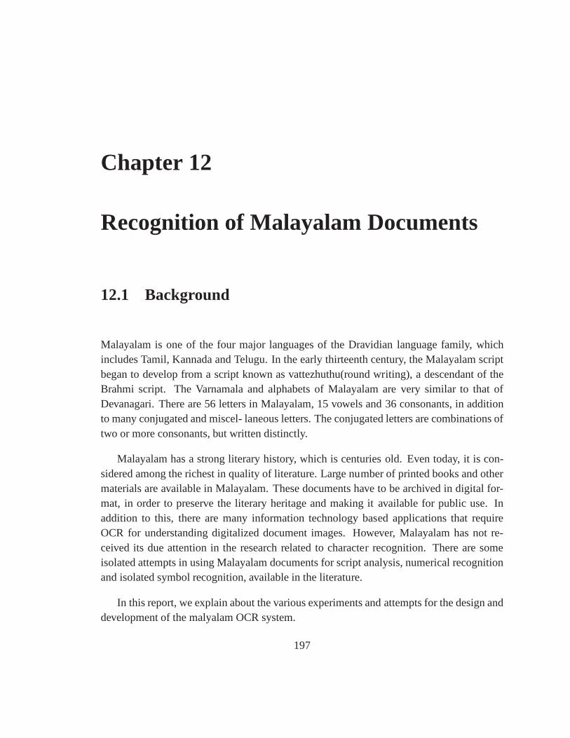
Chapter 12
Recognition of Malayalam Documents
12.1 Background
Malayalam is one of the four major languages of the Dravidianlanguage family, whichincludes Tamil, Kannada and Telugu. In the early thirteenthcentury, the Malayalam scriptbegan to develop from a script known as vattezhuthu(round writing), a descendant of theBrahmi script. The Varnamala and alphabets of Malayalam arevery similar to that ofDevanagari. There are 56 letters in Malayalam, 15 vowels and36 consonants, in additionto many conjugated and miscel- laneous letters. The conjugated letters are combinations oftwo or more consonants, but written distinctly.
Malayalam has a strong literary history, which is centuriesold. Even today, it is con-sidered among the richest in quality of literature. Large number of printed books and othermaterials are available in Malayalam. These documents haveto be archived in digital for-mat, in order to preserve the literary heritage and making itavailable for public use. Inaddition to this, there are many information technology based applications that requireOCR for understanding digitalized document images. However, Malayalam has not re-ceived its due attention in the research related to character recognition. There are someisolated attempts in using Malayalam documents for script analysis, numerical recognitionand isolated symbol recognition, available in the literature.
In this report, we explain about the various experiments andattempts for the design anddevelopment of the malyalam OCR system.
197
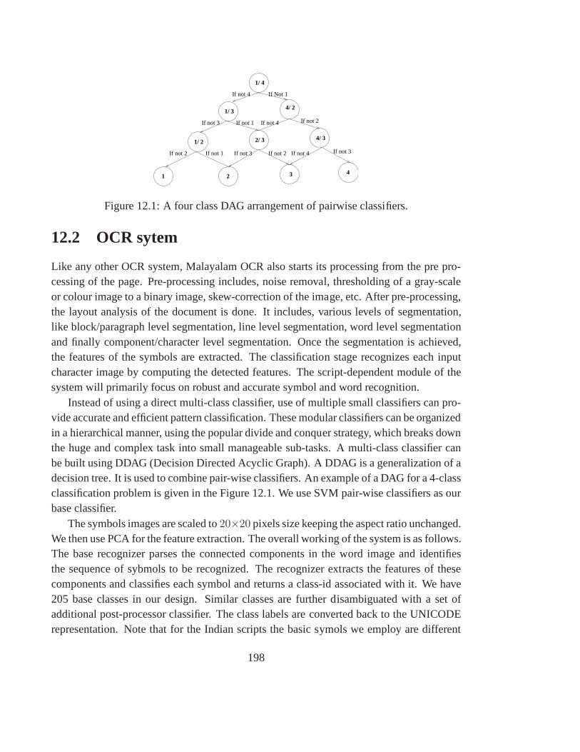
1/ 4
If not 4 If Not 1
2/ 3
If not 4If not 2If not 3If not 1If not 2 If not 3
1 24
4/ 31/ 2
1/ 34/ 2
If not 2If not 1If not 3 If not 4
3
Figure 12.1: A four class DAG arrangement of pairwise classifiers.
12.2 OCR sytem
Like any other OCR system, Malayalam OCR also starts its processing from the pre pro-cessing of the page. Pre-processing includes, noise removal, thresholding of a gray-scaleor colour image to a binary image, skew-correction of the image, etc. After pre-processing,the layout analysis of the document is done. It includes, various levels of segmentation,like block/paragraph level segmentation, line level segmentation, word level segmentationand finally component/character level segmentation. Once the segmentation is achieved,the features of the symbols are extracted. The classification stage recognizes each inputcharacter image by computing the detected features. The script-dependent module of thesystem will primarily focus on robust and accurate symbol and word recognition.
Instead of using a direct multi-class classifier, use of multiple small classifiers can pro-vide accurate and efficient pattern classification. These modular classifiers can be organizedin a hierarchical manner, using the popular divide and conquer strategy, which breaks downthe huge and complex task into small manageable sub-tasks. Amulti-class classifier canbe built using DDAG (Decision Directed Acyclic Graph). A DDAG is a generalization of adecision tree. It is used to combine pair-wise classifiers. An example of a DAG for a 4-classclassification problem is given in the Figure 12.1. We use SVMpair-wise classifiers as ourbase classifier.
The symbols images are scaled to20×20 pixels size keeping the aspect ratio unchanged.We then use PCA for the feature extraction. The overall working of the system is as follows.The base recognizer parses the connected components in the word image and identifiesthe sequence of sybmols to be recognized. The recognizer extracts the features of thesecomponents and classifies each symbol and returns a class-idassociated with it. We have205 base classes in our design. Similar classes are further disambiguated with a set ofadditional post-processor classifier. The class labels areconverted back to the UNICODErepresentation. Note that for the Indian scripts the basic symols we employ are different
198
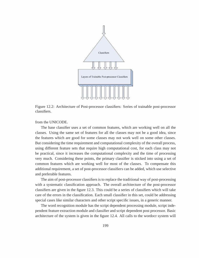
Figure 12.2: Architecture of Post-processor classifiers: Series of trainable post-processorclassifiers.
from the UNICODE.The base classifier uses a set of common features, which are working well on all the
classes. Using the same set of features for all the classes may not be a good idea, sincethe features which are good for some classes may not work wellon some other classes.But considering the time requirement and computational complexity of the overall process,using different feature sets that require high computational cost, for each class may notbe practical, since it increases the computational complexity and the time of processingvery much. Considering these points, the primary classifieris sticked into using a set ofcommon features which are working well for most of the classes. To compensate thisadditional requirement, a set of post-processor classifiers can be added, which use selectiveand preferable features.
The aim of post-processor classifiers is to replace the traditional way of post-processingwith a systematic classification approach. The overall architecture of the post-processorclassifiers are given in the figure 12.3. This could be a seriesof classifiers which will takecare of the errors in the classification. Each small classifier in this set, could be addressingspecial cases like similar characters and other script specific issues, in a generic manner.
The word recognition module has the script dependent processing module, script inde-pendent feature extraction module and classifier and scriptdependent post processor. Basicarchitecture of the system is given in the figure 12.4. All calls to the wordocr system will
199

Characters Confusing Merges Cuts
Classifier
Unicode
Verification Module
Post−processor Classifiers
Figure 12.3: Overall design of post-processor classifiers.
ScriptDependentProcessing
FeatureExtraction Classifier
Data dependent,Script Independent Learning Module
Post processingand converter
Data dependent,Script Dependent Learning Module
PreprocessedWord Image
Unicode(Obtained from the converter module)
Figure 12.4: Word Recognition Engine Architecture.
200
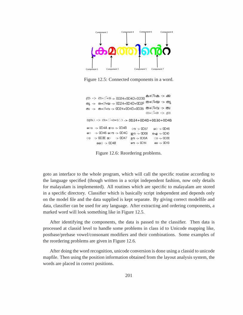
Figure 12.5: Connected components in a word.
Figure 12.6: Reordering problems.
goto an interface to the whole program, which will call the specific routine according tothe language specified (though written in a script independent fashion, now only detailsfor malayalam is implemented). All routines which are specific to malayalam are storedin a specific directory. Classifier which is basically scriptindependent and depends onlyon the model file and the data supplied is kept separate. By giving correct modelfile anddata, classifier can be used for any language. After extracting and ordering components, amarked word will look something like in Figure 12.5.
After identifying the components, the data is passed to the classifier. Then data isprocessed at classid level to handle some problems in class id to Unicode mapping like,postbase/prebase vowel/consonant modifiers and their combinations. Some examples ofthe reordering problems are given in Figure 12.6.
After doing the word recognition, unicode conversion is done using a classid to unicodemapfile. Then using the position information obtained from the layout analysis system, thewords are placed in correct positions.
201
12.3 Ongoing Activities
This section explains our recent attempts in improvement inperformance of the OCR sys-tem. In the present phase of the project, the following have been attempted:
• A first version of the OCR is integrated with the help of CDAC Noida. Some level ofexperimentation and testing is done. Some of the issues related to the OS (Fedora)to support the Malayalam specific fonts/displays are addressed. The focus has beenonly to output the correct UNICODE output.
• We use SVM classifier. However the scalability of the classifier system has been amajor bottleneck in this for character recognition applications where the number ofclasses could be very high. An appropriate data structure and the associated algo-rithms are designed to help the scalability for large class classification problems. Seenext section for some technical detail and experimental results on a generic characterclassification problem (not Malayalam). Note that the simplification does not affectthe classification accuracy.
• We studied the role of training data in design of high performing character classifica-tion systems. We trained the classifier with some font data (laboratory preparation)and then evaluated the test performance on the real-books inthe corpus. Later, weadded various percentages of the data into it and retrained.The performance contin-uously improved.
Our observation is that (i) The training data helps in improving the performancesignificantly. (ii) Corpus will have a significant role in enhancing the accuracy. (iii)A fixed reasonably small percentage of data from various print style may be used fortraining. (iv) Statistical feature selection techniques may be required for selectingsuitable features for a specific script.
• We designed a verification module as a possible post-processor to verify the recog-nized text by comparing them in the image space. This is done using a dynamicprogramming based technique.
Our observation is that (i) this provides a new method for post-processing and verifi-cation. (ii) this along with some language model could act asa feasible post processorstage for the Malayalam OCR.
• We also studied the performance of various classifiers and features for the classifica-tion task. Initial results of this is also provided. More comprehensive experimentsare being conducted.
202
12.3.1 Integration of OCR system
Due to the modularity of the code and simplicity of the system, integration of the Malay-alam OCR system with the GUI and other modules were done within hours. Only problemswe faced were, the output of the whole OCR was in html format for better formatting. Wehad to change that to ordinary text format. Some issues were related to the rendering ofMalayalam characters. Those issues were temporarily fixed using some patches to render-ing engine. It appears on later versions of Fedora and rendering engines these issues aresolved. They are more of OS level problems.
Since we made use of make for compilation, editing a line or two in the Makefilewas enough for generation of a shared library which can be plugged into the base system.Later on some bugs regarding reordering and document reconstruction were fixed. Sincethe files are stored in a well organized manner in standard unix style with Makefiles forcompilation, remote updation of the modules appeared pretty easy. Now, updation of thecode is going on on a regular basis till a central code repository is setup. After integration,we had updates on, layout analysis systems, improvements onclassifiers, script dependentwordocr modules and classid to unicode conversion module. All updates were sent to themand updation of code went without any trouble. Later on we areplanning to move to difffiles for easier management.
12.4 Efficient implementation of SVM
Directed Acyclic Graph with (1-Vs-1) binary SVM classifiers(DAGSVM) is proven toachieve the best accuracy for many multiclass problems. However, a bottleneck with thisapproach is the number of binary classifiers, and the associated space and time complex-ity. A multiclass data structure (MDS) is implemented for efficient multiclass solutions.We exploit the redundancies in support vectors across all the binary pairwise classifiers toobtain significant reduction in storage and computational requirements.
MDS for a N-class problem is shown in Figure 12.7. It consists of two major com-ponents. First one is a set of nodes, each of which representsa modifiedIPI(independentpair-wise implementation) node. Second one is a list of vectorsL, containingreducedsetof SVs for the multiclass problem. The effectiveness of our solution basically comes fromthe following change in the node structure. The first scalar arrayA in the node is retained assuch, while the second array of vectors that stored the SVs inthe original node are replacedwith a scalar arrayINDEX in MDS. This second array now stores the index positions ofthe corresponding SVs, that are moved to listL.
A direct implementation of DAG ideally treats the set of Support vectors (SVs) that
203
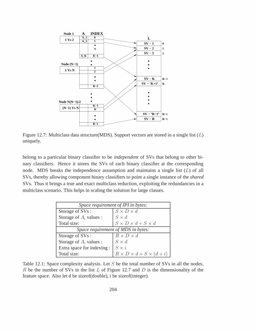
(N−1) Vs N
....
..
...
...
1 Vs 2
1 Vs N1
SV − 1
SV − 3SV − 2
A
SV − R
2
1
0
SV − ’R−1’
SV − ’K+1’SV − K K−1
K
R−1
R−2..R−1
KK−1
.2
.R−2
..10
K−1
Node 1
Node (N−1)
Node N(N−1)/2
INDEX
A_K
A_1A_2
L
Figure 12.7: Multiclass data structure(MDS). Support vectors are stored in a single list (L)uniquely.
belong to a particular binary classifier to beindependentof SVs that belong to other bi-nary classifiers. Hence it stores the SVs of each binary classifier at the correspondingnode. MDS breaks the independence assumption and maintainsa single list (L) of allSVs, thereby allowing component binary classifiers to pointa single instance of thesharedSVs. Thus it brings a true and exact multiclass reduction, exploiting the redundancies in amulticlass scenario. This helps in scaling the solution forlarge classes.
Space requirement of IPI in bytes:Storage of SVs : S ×D × dStorage ofAi values : S × dTotal size: S ×D × d + S × d
Space requirement of MDS in bytes:Storage of SVs : R ×D × dStorage ofAi values : S × dExtra space for indexing : S × iTotal size: R ×D × d + S × (d + i)
Table 12.1: Space complexity analysis. LetS be the total number of SVs in all the nodes,R be the number of SVs in the listL of Figure 12.7 andD is the dimensionality of thefeature space. Also let d be sizeof(double), i be sizeof(integer).
204

Table 12.1 summarizes the analysis of space required by IPI and MDS implementation.Though MDS adds an extra storage(S × i) for indexing, it is negligible considering theamount of reduction in the storage of SVs for large class problems. Our experiments showthat for a 300-class problemR is only 1% of S. As N increases, the space reductionapproachesS−R
S, since the space requirement ofA andINDEX are negligible compared
to that of support vectors.On a 300-class character recognition data set, a99% reduction in space and60% reduc-
tion in time are achieved, while preserving the accuracy exactly. The reduction in storageis achieved by the use of MDS and the reduction in time complexity is achieved by avodingthe duplicate kernel evaluations. The solution is very effective when the the no. of classesin the classification set is very large(in the order of hundreds). The pseudo code for theSVM classification, using this new datastrure is given in Algorithm 1. The experimentalresults showing the reduction in storage and time for 3 typesof kernels are shown in thetable 12.2.
Algorithm 1 SVM CLASSIFY(Node, Sample)1: for i = 1 to (Node→NumOfSVs)do2: index← (Node→ INDEX[i])3: if FLAG[index] = 0 then4: KERNEL[index]← K(Sample, L[index])5: FLAG[index]← 16: end if7: Add KERNEL[index] × (Node→ A[i]) to D8: end for9: Add (Node→ b) to D
10: RETURNsign of D11: END SVM CLASSIFY
12.5 Ongoing and Future Activities
• Completion of empirical analysis with focus on selection ofbetter features and clas-sification analysis.
• Enhancement of post-processor classifiers and use of other techniques for postpro-cessing.
• Addressing cuts and merges in the recognition phase.
205
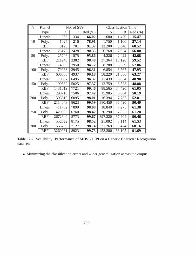
N Kernel No. of SVs Classification TimeType S R Red.(%) S R Red.(%)
10Linear 983 334 66.02 1.680 1.420 15.47Poly. 1024 216 78.91 1.750 1.100 37.14RBF 8123 701 91.37 12.200 3.840 68.52
50Linear 25172 2428 90.35 6.768 2.924 56.80Poly. 25706 1575 95.86 4.226 2.422 42.68RBF 211948 3382 98.40 37.364 15.126 59.52
100Linear 74855 3950 94.72 8.288 3.559 57.06Poly. 79963 2945 96.31 6.854 3.567 47.95RBF 606058 4937 99.18 58.220 21.386 63.27
150Linear 178857 6495 96.37 11.439 5.834 48.98Poly. 190832 5025 97.37 12.759 6.523 48.88RBF 1431019 7721 99.46 88.565 34.490 61.05
200Linear 290716 7506 97.42 15.985 6.684 58.19Poly. 306619 6095 98.01 16.394 7.737 52.81RBF 2114043 8623 99.59 380.450 36.490 90.40
250Linear 411732 7899 98.08 18.840 7.275 61.38Poly. 429006 6760 98.42 20.290 7.855 61.28RBF 2672340 8773 99.67 397.320 37.904 90.46
300Linear 552622 8175 98.52 21.092 8.114 61.53Poly. 566709 7127 98.74 21.269 8.474 60.16RBF 3260961 8923 99.73 458.280 38.105 91.69
Table 12.2: Scalability: Performance of MDS Vs IPI on a Generic Character Recognitiondata set.
• Minimizing the classification errors and wider generalization across the corpus.
206
Chapter 13
Language Resources for correcting OCRoutput
This chapter describes the techniques proposed for improving accuracy of OCR output us-ing lexical resources. In particular, we describe script specific post-processing techniquewith particular reference to Devnagari script. It also discusses how language models canbe used as post-processing resources. Finally, it also examines effectiveness of using elec-tronic dictionary for the correction of recognition results.
13.1 Introduction
Processing of images of document pages is becoming increasingly important for applica-tions to office and library automation, e-governance, postal services etc. The procedure forautomatically processing the text components of a complex document which contain text,graphics and/or images can be divided into three stages:
i) Document layout analysis for extraction of text regionii) Text line, possibly word and symbol / character recognition
iii) Optical character / symbol recognition
The output of the recognition engine can be further processed using target language orcorpora based lexical recourses for reducing errors in recognition.
Although commercial system are available for Roman, Cyrillic, for east as well as mid-dle eastern languages, such systems for Indian scripts are still under development. Indianscripts because of their unique nature pose a different kindof technical challenge. In thispaper we shall discus how post-processing of OCR output can be used in the context ofIndian languages for improving accuracy of the results.
207
13.2 Indian Scripts
In India, there are more than eighteen official (Indian Constitution accepted) languages.These are: Assamese, Bangla, English,Gujarati, Hindi, Kankani, Kannada, Kashmiri, Malay-alam, Marathi, Nepali, Oriya, Punjabi, Rajasthani, Sanskrit, Tamil, Telugu and Urdu.Twelve different scripts are used for writing these languages. Hence, we need twelvedifferent script dependent OCRs to cater to the needs of these official languages. Since,post-processing depends upon language characteristics, we need to develop post-processingtools for each of these languages.
Most Indian scripts have originated from ancient Brahmi through various transforma-tions. Apart from vowel and consonant characters, there arecompound characters in mostIndian script system with the exception of Tamil and Gurumukhi. The shape of a com-pound character is usually more complex than the constituent characters. In general, thereare about 300 symbol shapes in an Indian script.
13.3 Related Work
There has been considerable research on automatically correcting words in text in general,and correction of OCR output in particular. Kukich (1992) [47] provides a general surveyof the research in the area. Unfortunately, there is no commonly used evaluation base forOCR error correction, making comparison of experimental results difficult. Some systemsintegrate the post-processor with the actual character recognizer to allow interaction be-tween the two. In an early study, Hanson et al. (1976) [48] reports a word error rate ofabout 2% and a reject rate of 1%, without a dictionary. Sinha and Prasada (1988) [49]achieve 97% word recognition, ignoring punctuation, usingan aug- mented dictionary, aViterbi style algorithm, and manual heuristics. Many systems treat OCR as a black box,generally employing word and/or character leveln-grams along with character confusionprobabilities. Srihari et al. (1983) [29] is one typical example and reports up to 87% er-ror correction on artificial data, relying (as we do) on a lexicon for correction. Goshtasbyand Ehrich (1988) [50] presents a method based on probabilistic relaxation labeling, usingcontext characters to constrain the probability of each character. They do not use a lexiconbut do require the probabilities assigned to individual characters by the OCR system. Joneset al. (1991) [51] describe an OCR post-processing system comparable to ours, and reporterror reductions of 70-90%. Their system is designed arounda stratified algorithm. Thefirst phase performs isolated word correction using rewriterules, allowing words that arenot in the lexicon. The second phase attempts correcting word split errors, and the lastphase uses word bigram probabilities to improve correction. The three phases interact with
208
each other to guide the search. In comparison to our work, themain difference is our focuson an end-to-end generative model versus their stratified algorithm centered around correc-tion. Perez-Cortes et al. (2000) [52] describes a system that uses a stochastic FSM thataccepts the smallest k-testable language consistent with arepresentative language sample.Depending on the value of k, correction can be restricted to sample language, or variationsmay be allowed. They report reducing error rate from 33% to below 2% on OCR outputof hand-written Spanish names from forms. Pal et al. (2000) [53] describes a methodfor OCR error correction of an inflectional Indian language using morphological parsing,and reports correcting 84% of the words with a single character error. Although it is lim-ited to single errors, the system demonstrates the possibility of correcting OCR errors inmorphologically rich languages.
Taghva and Stofsky (2001) [54] takes a different approach topost-processing and pro-poses an interactive spelling correction system specifically designed for OCR error cor-rection. The system uses multiple information resources topropose correction candidatesand lets the user review the candidates and make corrections. Although segmentation er-rors have been addressed to some degree in previous work, to the best of our knowledgeour model is the first that explicitly incorporates segmentation. Similarly, many systemsmake use of a language model, a character confusion model, etc., but none have developedan end-to-end model that formally describes the OCR processfrom the generation of thetrue word sequence to the output of the OCR system in a manner that allows for statisticalparameter estimation. Our model is also the first to explicitly model the conversion of asequence of words into a character sequence.
Unfortunately, the output of commercial OCR systems is far from perfect, especiallywhen the language in question is resource-poor (Kanungo et al., in revision [55]). Andefforts to acquire new language resources from hardcopy using OCR (Doermann et al [56])face something of a chicken-and-egg problem. The problem iscompounded by the factthat most OCR system are black boxes that do not allow user tuning or re-training – Baird(1999, reported in (Frederking, 1999) [57]) comments that the lack of ability to rapidlyretarget OCR/NLP applications to new languages is “largelydue to the monolithic structureof current OCR technology, where language-specific constraints are deeply enmeshed withall the other code.”
Kolak et al [1] describe a complete probabilistic, generative model for OCR, motivatedspecifically by
(a) the need to deal with monolithic OCR systems,(b) the focus on OCR as a component in NLP applications, and(c) the ultimate goal of using OCR to help acquire resources for new languages fromprinted text.
209
After presenting the model itself, we discuss the model’s implementation, training, and itsuse for post-OCR error correction. then present an evaluation for standalone OCR correc-tion.
13.4 The Model (Kolak et al [1])
Generative “noisy channel” models relate an observable string O to an underlying se-quence, in this case recognized character strings and underlying word sequencesW Thisrelationship is modeled byP (W, O) decomposed by Bayes’s Rule into steps modeled byP (W ) (the source model) andP (O|W ) (comprising sub-steps generatingO from W . Eachstep and sub-step is completely modular, so one can flexibly make use of existing submod-els or devise new ones as necessary. We begin with preliminary definitions and notation.A true word sequence〈W1, ..., Wr〉 corresponds to a true character sequence.〈C1, ..., Cn〉,and the OCR system’s output character sequence is given by〈O1, ..., On〉.
A segmentation of the true character sequence intop subsequences is represented as〈C1, ..., Cp〉. Segment boundaries are only allowed between characters. Subsequences aredenoted using segmentation positionsa = 〈a1, ...ap−1〉 whereai < ai+1 a0 = 0, ap = n.
Theai define character sequences〈Cai−1, ..., Cai
〉. The number of segmentsp need notequal the number of wordsr andCi need not be a word inW .
Correspondingly, a segmentation of the OCR’d character sequence intoq subsequencesis given by〈O1, ..., Oq〉. Subsequences are denoted byb = 〈b1, ...bq−1〉, wherebj < bj+1,b0 = 0, andbq = m. Theb define character sub-sequencesOj = (Obj−1
, ..., Obj]. Align-
ment chunks are pairs of corresponding truth and OCR subsequences:〈Oi, Ci〉, i = 1, ..., p.The model is easily modified to permitp 6= q.
− The first step in transformingW to O is generation of a character sequenceC, modeledasP (C|W ). This step accommodates the character-based nature of OCR system, andprovides a place to model the mapping of different charactersequences to the sameword sequence (case/font variation) or vice versa (e.g. ambiguous word segmentationin Chinese).
− Segmentation:SubsequencesCi are generated fromC by choosing a set of boundary positions,a. Thissub-step, modeled byP (a|C, W ), is motivated by the fact that most OCR systems firstperform image segmentation, and then perform recognition on a word by word basis.For a language with clear word boundaries (or reliable tokenization or segmentationalgorithms), one could simply use spaces to segment the character sequence in a non-probabilistic way. However, OCR systems may make segmentation errors and resulting
210
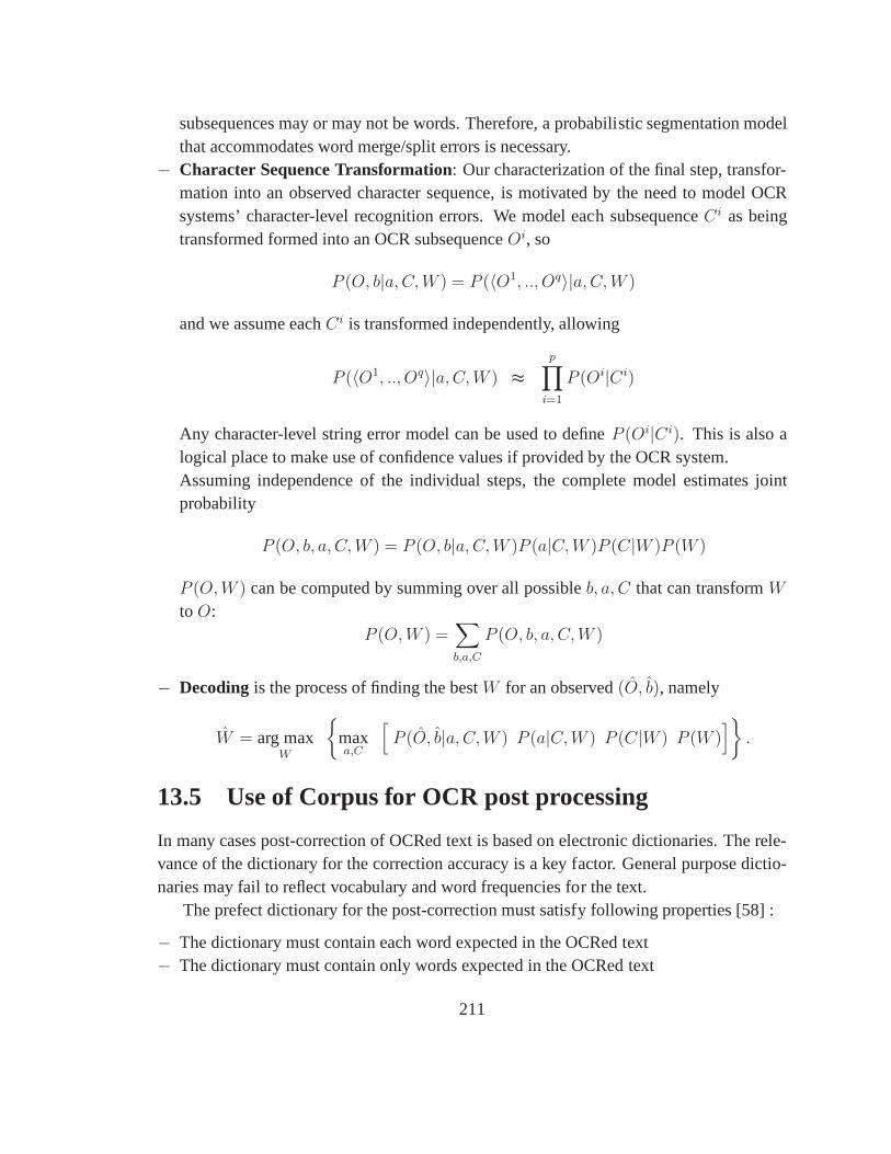
subsequences may or may not be words. Therefore, a probabilistic segmentation modelthat accommodates word merge/split errors is necessary.
− Character Sequence Transformation: Our characterization of the final step, transfor-mation into an observed character sequence, is motivated bythe need to model OCRsystems’ character-level recognition errors. We model each subsequenceCi as beingtransformed formed into an OCR subsequenceOi, so
P (O, b|a, C, W ) = P (〈O1, .., Oq〉|a, C, W )
and we assume eachCi is transformed independently, allowing
P (〈O1, .., Oq〉|a, C, W ) ≈
p∏
i=1
P (Oi|Ci)
Any character-level string error model can be used to defineP (Oi|Ci). This is also alogical place to make use of confidence values if provided by the OCR system.Assuming independence of the individual steps, the complete model estimates jointprobability
P (O, b, a, C, W ) = P (O, b|a, C, W )P (a|C, W )P (C|W )P (W )
P (O, W ) can be computed by summing over all possibleb, a, C that can transformWto O:
P (O, W ) =∑
b,a,C
P (O, b, a, C, W )
− Decodingis the process of finding the bestW for an observed(O, b), namely
W = arg maxW
{
maxa,C
[
P (O, b|a, C, W ) P (a|C, W ) P (C|W ) P (W )]
}
.
13.5 Use of Corpus for OCR post processing
In many cases post-correction of OCRed text is based on electronic dictionaries. The rele-vance of the dictionary for the correction accuracy is a key factor. General purpose dictio-naries may fail to reflect vocabulary and word frequencies for the text.
The prefect dictionary for the post-correction must satisfy following properties [58] :
− The dictionary must contain each word expected in the OCRed text− The dictionary must contain only words expected in the OCRedtext
211
− For each word, dictionary must store expected probability of occurrence of a word Wwith reference to the domain of the documents being OCRed.
In practice, perfect dictionary is not available. To satisfy property 1, it is sometimesrecommended to use a large-scale dictionary which contain amaximal collection of words.Other option is that of using a dictionary that contains mostcommon tokens. However inall these cases dictionary is not adapted to the given thematic topic.
Consider a corpus C of documents and a dictionary D. We can define lexical coverageof a given dictionary D as the percentage of normal words/tokens of C that are in D. Wecan use the dictionary D in the following way for correcting OCR output: Let Wo denoteOCR output word and Wc denote corrected output word. 1.We canfix an upper-bound Bofor the length sensitive edit distance between Wo and candidate Wcs from the dictionary;we also define a threshold Po for the probability of occurrence of the candidate Wcs fromthe dictionary. 2.For a given Wo, we find a set of matches in thedictionary using editdistance as the match measure. If we do not have a perfect match (i.e edit distance is notzero), consider the ones at minimal edit distance from Wo. Among these matches we selectthe one having maximum probability of occurrence for the given corpus. 3.If the selectedmatch in step 2 satisfies the constraints of step 1, we correctWo by the selected match Wc.
It is clear from the above discussion that pure dictionary based techniques do not makeuse of sentence level grammatical model of the languages or language dependent rules forword formation.
13.5.1 Gurmukhi
In order to rectify the classification errors, the output of classification stage will be fed tothe post processor. For the post processing we will ues at 10 million word Punjabi corpus,which will serve the dual purpose of providing data for statistical analysis of Punjabi lan-guage and also for checking the spelling of a word. The unigram, bigram and trigram tablesextracted from the corpus will be used to decide between confusing words and characters.Punjabi grammar rules will also be incorporated to check forillegal character combinationssuch as presence of two consecutive vowels or a word startingwith a forbidden consonantor vowel.
13.6 Conclusions
In this chapter we have provided a brief introduction to the techniques that can be used forcorrection of OCR errors using language and script based resources. Application of these
212

techniques for Indian scripts and languages require formulation of appropriate languageand script models. A sufficiently large corpora of ground-truthed data can only supportsuch development.
213


Chapter 14
Software Engineering : Integration andNamespaces
14.1 Deliverables
A) Software Development Kit (SDK) for each module of the OCR.This would allowthe use of developed algorithms and methodologies to be usedfor developing OCRsfor other scripts (not addressed in this project) as well.
B) The software will be delivered as an OCR package (DLL for windows and shared-object library for linux). Thus it can be used as a stand-alone application also.
C) A user-interface will be provided to the complete OCR system. This would beused for presentation purpose− viewing, editing of documents and conversion toalternate document formats. Interface can also be providedto individual modulesso that intermediate outputs can be examined.
14.2 Software Environment
− Inter mixing of new and malloc for memory allocation can cause problem and difficultto debug.
− Internal Linking for C and C++ Code will be different and we may have to explic-itly define “extern C linkage” for C++ Code. The following link describes it in detail.http://www.parashift.com/c++-faq-lite/mixing-c-and-cpp.html
− Process of converting C++ Code to Shared Library will be different (Approach can besimilar to that of development of STL(Standard Template Library)).
− CDAC Noida has developed the process of converting C Code to shared Library and is
215

working for Fedora 3.(And it will be same for Fedora 6).
There can be many more problems which will be different from compiler to compiler. Forthis reason we like to suggest the released code to be in ANSI C++.
14.3 System Integration
14.3.1 System Integration Architecture
We will use the Broker Architecture for the integration of the APIs developed by the con-sortium members. The architecture is described below.
Broker enables autonomous and heterogeneous systems to share information whilemaintaining autonomous control.
The following items are the key components of the Broker concept:− Each system interfaces with the Broker and does not exchangeany information directly
with other systems.− Each system can interface with the Broker in whatever formatthe system is designed to
support.− Data received by the Broker are examined, translated into neutral format, and forwarded
to the appropriate system(s).− The Broker does some error checking and may request retransmissions.The Broker architecture as explained by the diagram Figure 14.1 depicts that if there isany communication between three modules that needs to be integrated, then the way ofcommuting between two modules is using a middle-ware shown here as a broker. It is thebroker, which gives input to one system and accepts its output and makes it as an input toanother system.
System 1
Broker
System 3
System 2
Figure 14.1: Broker Architecture for system Integration
The process or the flow of the integration would follow certain steps, which are describedbelow:
216
− The first step would be to collect the API details from each of the consortium membersusing template in Fig 14.3. We will analyze the various interface modalities that all the11 consortium members are planning to develop. A broad picture of the interface shouldbe designed by each of the members, which would describe the functional requirementsof the system with their parameters and data type values. Theinputs to the interface andthe outputs of the system should be clearly mentioned with asmuch intricate detailingas possible.
− After individually studying each of the interfacing modalities we would look if the out-put produced from one module satisfies the conditions of becoming as the input of thesecond module.
− If there are any discrepancies between the two modules whichneeds to interact witheach other then template (Fig 14.4) will be used to suggest changes and modificationsto one another. This template will be delivered to both the institutions and throughrepeated interactions with each; these inconsistencies inthe system would be resolved.
− The next step towards integration would be to identify the major sub-systems (whichmay include one or more APIs interacting with each other) that can be identified from allthe organizations building their individual APIs, and building a GUI for its integrationtesting.
− We will than have Integration Test Plan to test the interfaces between the APIs througha GUI based integrated system.
14.3.2 Integration Testing
It is the phase of software testing in which individual software modules are combined andtested as a group. It follows unit testing and precedes system testing. Integration testingtakes as its input modules that have been checked out by unit testing, groups them in largeraggregates, applies tests defined in an Integration test plan to those aggregates, and deliversas its output the integrated system ready for system testing. Integration Testing essentiallymeans testing the modules individually to see if the moduleswork in accordance with thedesired output being sought after and then making it work in co-ordination with other mod-ules as well so as to see that it builds the system as a whole by just using inputs and outputsof one module as input and outputs of the other module. Integration testing of software isdifficult because they tend to be large and complex; it is often structured as a set of taskswhose interaction patterns can be arbitrary and non deterministic. The problem is to in-tegrate components, each of which functions properly into one larger system, satisfyingthe combined requirements within the newly formed environment Integration testing canproceed in a number of different ways, which can be broadly characterized as topdown
217
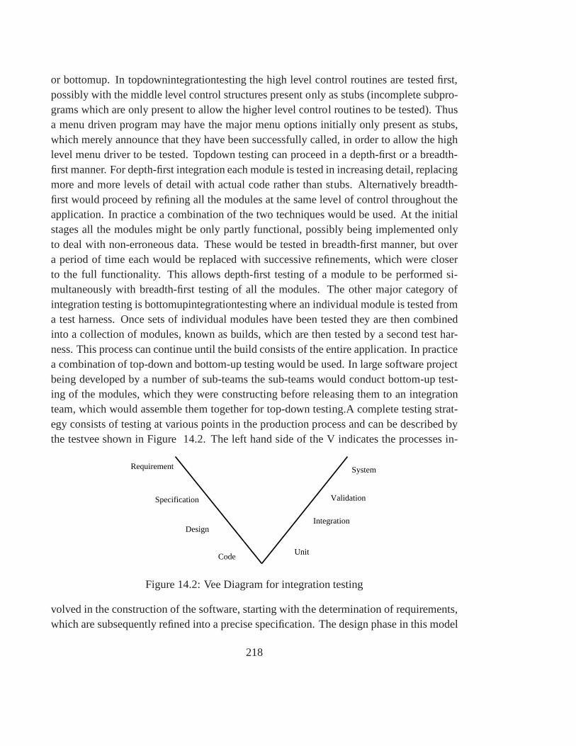
or bottomup. In topdownintegrationtesting the high level control routines are tested first,possibly with the middle level control structures present only as stubs (incomplete subpro-grams which are only present to allow the higher level control routines to be tested). Thusa menu driven program may have the major menu options initially only present as stubs,which merely announce that they have been successfully called, in order to allow the highlevel menu driver to be tested. Topdown testing can proceed in a depth-first or a breadth-first manner. For depth-first integration each module is tested in increasing detail, replacingmore and more levels of detail with actual code rather than stubs. Alternatively breadth-first would proceed by refining all the modules at the same level of control throughout theapplication. In practice a combination of the two techniques would be used. At the initialstages all the modules might be only partly functional, possibly being implemented onlyto deal with non-erroneous data. These would be tested in breadth-first manner, but overa period of time each would be replaced with successive refinements, which were closerto the full functionality. This allows depth-first testing of a module to be performed si-multaneously with breadth-first testing of all the modules.The other major category ofintegration testing is bottomupintegrationtesting wherean individual module is tested froma test harness. Once sets of individual modules have been tested they are then combinedinto a collection of modules, known as builds, which are thentested by a second test har-ness. This process can continue until the build consists of the entire application. In practicea combination of top-down and bottom-up testing would be used. In large software projectbeing developed by a number of sub-teams the sub-teams wouldconduct bottom-up test-ing of the modules, which they were constructing before releasing them to an integrationteam, which would assemble them together for top-down testing.A complete testing strat-egy consists of testing at various points in the production process and can be described bythe testvee shown in Figure 14.2. The left hand side of the V indicates the processes in-
Requirement
Specification
Design
Code
System
Validation
Integration
Unit
Figure 14.2: Vee Diagram for integration testing
volved in the construction of the software, starting with the determination of requirements,which are subsequently refined into a precise specification.The design phase in this model
218
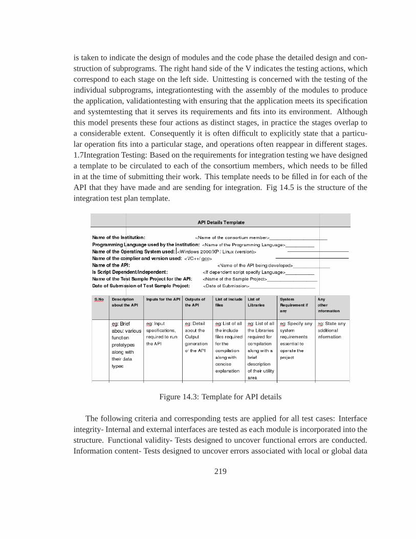
is taken to indicate the design of modules and the code phase the detailed design and con-struction of subprograms. The right hand side of the V indicates the testing actions, whichcorrespond to each stage on the left side. Unittesting is concerned with the testing of theindividual subprograms, integrationtesting with the assembly of the modules to producethe application, validationtesting with ensuring that theapplication meets its specificationand systemtesting that it serves its requirements and fits into its environment. Althoughthis model presents these four actions as distinct stages, in practice the stages overlap toa considerable extent. Consequently it is often difficult toexplicitly state that a particu-lar operation fits into a particular stage, and operations often reappear in different stages.1.7Integration Testing: Based on the requirements for integration testing we have designeda template to be circulated to each of the consortium members, which needs to be filledin at the time of submitting their work. This template needs to be filled in for each of theAPI that they have made and are sending for integration. Fig 14.5 is the structure of theintegration test plan template.
Figure 14.3: Template for API details
The following criteria and corresponding tests are appliedfor all test cases: Interfaceintegrity- Internal and external interfaces are tested as each module is incorporated into thestructure. Functional validity- Tests designed to uncoverfunctional errors are conducted.Information content- Tests designed to uncover errors associated with local or global data
219
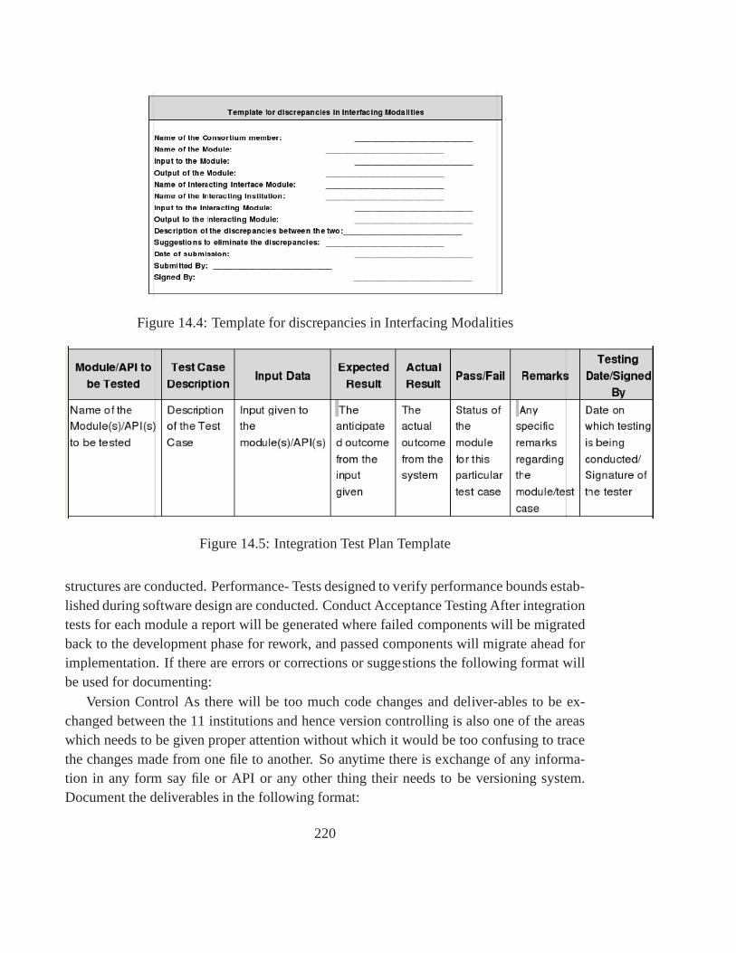
Figure 14.4: Template for discrepancies in Interfacing Modalities
Figure 14.5: Integration Test Plan Template
structures are conducted. Performance- Tests designed to verify performance bounds estab-lished during software design are conducted. Conduct Acceptance Testing After integrationtests for each module a report will be generated where failedcomponents will be migratedback to the development phase for rework, and passed components will migrate ahead forimplementation. If there are errors or corrections or suggestions the following format willbe used for documenting:
Version Control As there will be too much code changes and deliver-ables to be ex-changed between the 11 institutions and hence version controlling is also one of the areaswhich needs to be given proper attention without which it would be too confusing to tracethe changes made from one file to another. So anytime there is exchange of any informa-tion in any form say file or API or any other thing their needs tobe versioning system.Document the deliverables in the following format:
220

Figure 14.6: Template for Error Correction/Suggestion
Here in this version controlling document the date of delivery of the changed deliv-ery, the new version number of the deliverable, the author orthe organization which hasimplemented the changes, the module or the section for whichthe changes has been doneand in amendment document the specific changes that have beenmade in that particularmodule/section.
Figure 14.7: Template for Version Control
221
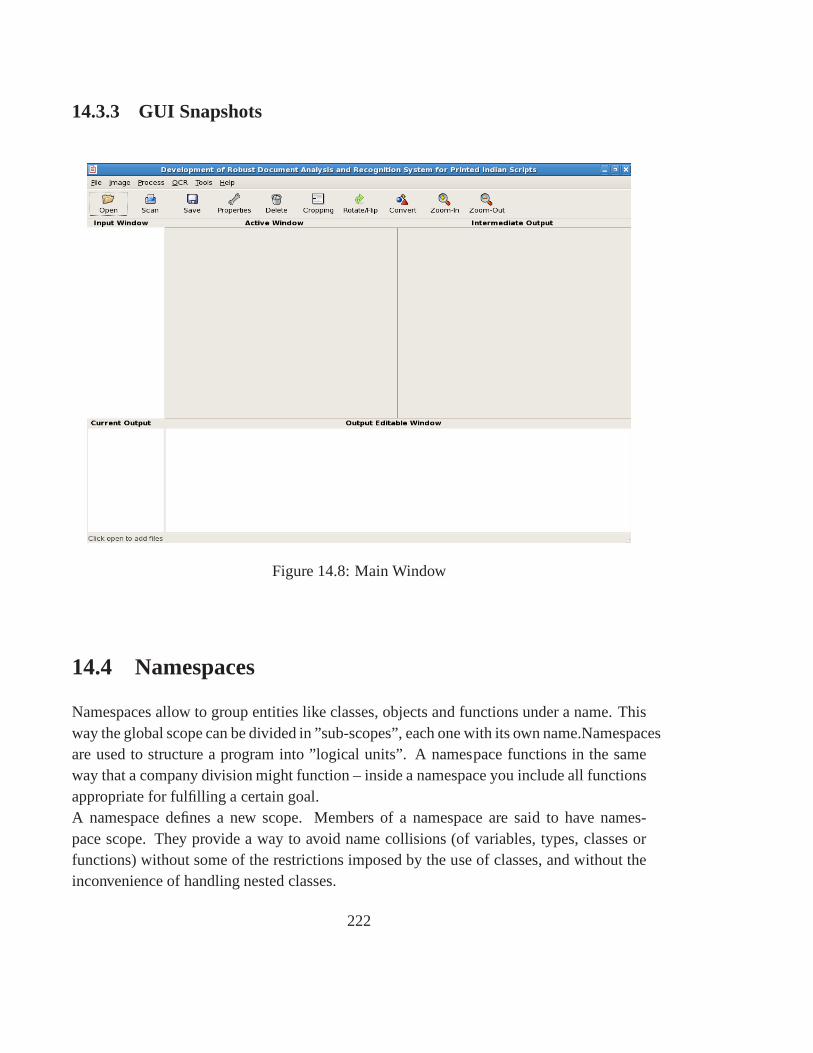
14.3.3 GUI Snapshots
Figure 14.8: Main Window
14.4 Namespaces
Namespaces allow to group entities like classes, objects and functions under a name. Thisway the global scope can be divided in ”sub-scopes”, each onewith its own name.Namespacesare used to structure a program into ”logical units”. A namespace functions in the sameway that a company division might function – inside a namespace you include all functionsappropriate for fulfilling a certain goal.A namespace defines a new scope. Members of a namespace are said to have names-pace scope. They provide a way to avoid name collisions (of variables, types, classes orfunctions) without some of the restrictions imposed by the use of classes, and without theinconvenience of handling nested classes.
222
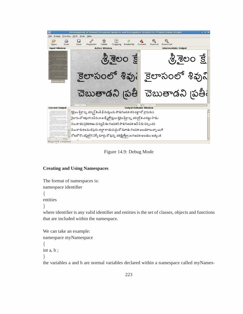
Figure 14.9: Debug Mode
Creating and Using Namespaces
The format of namespaces is:namespace identifier{entities}where identifier is any valid identifier and entities is the set of classes, objects and functionsthat are included within the namespace.
We can take an example:namespace myNamespace{int a, b ;}the variables a and b are normal variables declared within a namespace called myNames-
223

Figure 14.10: NonDebug Mode
pace. In order to access these variables from outside the myNamespace namespace we haveto use the scope operator ::. For example, to access the previous variables from outside my-Namespace we can write:
myNamespace::amyNamespace::b
Another way to use the namespace is to introduce an entire namespace into a section ofcode by using the syntax:using namespace myNamespace ;Doing so will allow the programmer to call functions from within the namespace withouthaving to specify the namespace of the function while in the current scope. (Generally,until the next closing bracket, or the entire file, if you aren’t inside a block of code.) Thisconvenience can be abused by using a namespace globally, which defeats some of the pur-pose of using a namespace.A common example of this usage is:
224
using namespace std ;which grants access to the std namespace that includes C++ I/O objects cout and cin.
The convention to be used in this project isnamespaceInstitutename Modulename;
Nesting Namespaces
Nesting a namespace is the ability to include a namespace inside (as part of the body) ofanother namespace. To do this, create the intended namespace as a member of the parentnamespace. The nested namespace should have its own name andits own body. Here is anexample:namespace BuyAndSell{double originalPrice;double taxRate;double taxAmount;double discount;double discountAmount;double netPrice;namespace item{long itemNumber;}}
The std Namespace
To avoid name conflicts of the various items used in its own implementation, the C++Standard provides a namespace called std. The std namespaceincludes a series of librariesthat you will routinely and regularly use in your programs.
Therefore, whenever you need to use a library that is part of the std namespace, insteadof typing a library with its file extension, as in iostream.h,simply type the name of thelibrary as in iostream. Then, on the second line, type using namespace std;
As an example, instead of typing#include ¡iostream.h¿
225
You can type:#include ¡iostream¿using namespace std;
Because this second technique is conform with the C++ Standard, we will use it when-ever we need one of its libraries.
Unnamed Namespaces
We can also declare unnamed namespaces. For example:namespace{class Car{.... // class members here}// other members here}this definition behaves exactly like:
namespace UniqueName{class Car{.... // class members here}// other members here}using namespace UniqueName;For each unnamed namespace, the compiler generates a uniquename (represented here byUniqueName), which differs from every other name in the program.
Advantages of using Namespaces
1. By enabling this program structure, C++ makes it easier for you to divide up a pro-gram into groups that each perform their own separate functions, in the same way thatclasses or structs simplify object oriented design. But namespaces, unlike classes, donot require instantiation you do not need an object to use a specific namespace. You
226

only need to prefix the function you wish to call with namespace name :: similar tohow you would call a static member function of a class.
2. Another convenience of namespaces is that they allow you to use the same functionname, when it makes sense to do so, to perform multiple different actions.
227

Chapter 15
ASSESSMENT OF OCR SOFTWARE
15.1 Introduction
Software quality measures how well the software is designedand how well software con-firms to that design. The standard ISO9126 quality model defines a set of software qualitycharacteristics and sub characteristics. ISO9126 presents three different views of quality-internals and externals views along with quality in use. Characteristics of internal andexternal quality are the following:
1. Functionality
2. Reliability
3. Usability
4. Efficiency
5. Maintainability
6. Portability
Quality in use is characterized by
1. Effectiveness
2. Productivity
3. Safety
4. Satisfaction
229
In the ISO quality model, a software quality is defined as a category of software quality at-tributes that influence software quality. An attribute is a measurable property. This impliesthat software quality can be specified in terms of these attribute values after identifyingrelevant attributes for the class of software under consideration.
As per ISO9126, functionalitys five sub characteristics are
(i) suitability
(ii) accuracy
(iii) inter operability
(iv) security
(v) compliance.
In the context of a OCR system applicable features for which we need to define metricsare:
(a) suitability
(b) accuracy
(c) inter operability.
Similarly for efficiencys sub characteristics specific measures need to be defined for (i)Time behavior & (ii) resource utilisation. With reference to Reliability , Usability, Main-tainability & Portability we need to examine applicabilityof standard software metrics.
15.2 OCR Software Testing & Quality Assessment
Testing is an integral part in software development. Basic purpose of testing is to (i) im-prove quality of the software (ii) verification & validation. We cannot measure qualitydirectly but we can test related factors to make it visible.
Tests with the purpose of validating the product works are named clean tests, or positivetests. The drawbacks are that it can only validate that the software works for the specifiedtest cases. A finite number of tests cannot validate that the software works for all situations.On the contrary, only one failed test is sufficient enough to show that the software does notwork.
Software reliability has important relations with many aspects of software, includingthe structure, and the amount of testing it has been subjected to. Based on an operational
230
profile (an estimate of the relative frequency of use of various inputs to the program), testingcan serve as a statistical sampling method to gain failure data for reliability estimation.
There is a plethora of testing methods and testing techniques, serving multiple purposesin different life cycle phases. Classified by purpose, software testing can be divided into:correctness testing, performance testing, reliability testing and security testing. In case ofour OCR software only first three testing modalities are relevant. Of these reliability testingcan be attempted only after satisfactory completion of the first two testing process.
15.3 Correctness testing
Correctness is the minimum requirement of software, the essential purpose of testing. Cor-rectness testing will need some type of oracle, to tell the right behavior from the wrongone. The tester may or may not know the inside details of the software module under test,e.g. control flow, data flow, etc.
15.3.1 Black-box testing
The black-box approach is a testing method in which test dataare derived from the specifiedfunctional requirements without regard to the final programstructure. It is also termed data-driven, input/output driven, or requirements-based testing. Because only the functionalityof the software module is of concern, black-box testing alsomainly refers to functionaltesting – a testing method emphasized on executing the functions and examination of theirinput and output data. The tester treats the software under test as a black box – onlythe inputs, outputs and specification are visible, and the functionality is determined byobserving the outputs to corresponding inputs. In testing,various inputs are exercised andthe outputs are compared against specification to validate the correctness. All test cases arederived from the specification. No implementation details of the code are considered.
For the OCR system, black box testing is applicable to modules as well as to the inte-grated system. In other words, basic unit testing and integration testing is formulated asblack box testing. In the OCR system, for each module we have the specification of theinput and output data defined in unambiguous fashion throughXML tag structure. Hence,the procedure followed for black box testing of each module is :
1. Prepare input data as per XML specification. XML parser canbe used for validationof the input data.
2. Provide input data to the module.
231
3. For a given input data, exercise the module for different values of input parameters,if any
4. Check for validity of the output as per XML specification ofthe output
Input data is to be prepared from the corpus generated for theproject by random sam-pling of the collection. The objective of the testing will beto make sure that the modulesexecute as per the functionality defined and produce valid output for different inputs. Animportant aspect to explore is that software satisfies the condition of graceful degradationand has the ability to handle exceptions. Black box testing process is not expected to eval-uate accuracy or generate performance metric.
In order to test the integrated system, black box testing process will involve testing ofthe inbuilt workflows of different script specific OCRs. Since, the OCR system can executedifferent combination of functional modules, black box testing needs to consider only validcombinations as defined in the workflow of individual OCRs.
It is obvious that the more we have covered in the input space,the more problems wewill find and therefore we will be more confident about the quality of the software. Ideallywe would be tempted to exhaustively test the input space. Butas stated above, exhaustivelytesting the combinations of valid inputs will be impossiblefor OCR,let alone consideringinvalid inputs, timing, sequence, and resource variables.Combinatorial explosion is themajor roadblock in functional testing. A good testing plan will not only contain black-boxtesting, but also white-box approaches, and combinations of the two.
15.3.2 White-box testing
Contrary to black-box testing, software is viewed as a white-box, or glass-box in white-box testing, as the structure and flow of the software under test are visible to the tester.Testing plans are made according to the details of the software implementation, such asprogramming language, logic, and styles. Test cases are derived from the program struc-ture. White-box testing is also called glass-box testing, logic-driven testing or design-basedtesting. There are many techniques available in white-box testing, because the problem ofintractability is eased by specific knowledge and attentionon the structure of the softwareunder test. The intention of exhausting some aspect of the software is still strong in white-box testing, and some degree of exhaustion can be achieved, such as executing each lineof code at least once (statement coverage), traverse every branch statements (branch cover-age), or cover all the possible combinations of true and false condition predicates (Multiplecondition coverage). Control-flow testing, loop testing, and data-flow testing, all maps thecorresponding flow structure of the software into a directedgraph. Test cases are carefully
232
selected based on the criterion that all the nodes or paths are covered or traversed at leastonce. By doing so we may discover unnecessary ”dead” code – code that is of no use,or never get executed at all, which cannot be discovered by functional testing. Since, thevolume of code is large, even for each functional module, it is impossible to do exhaustivetesting. It is expected that white box testing is to be carried out only with reference to thetop level structure of the software. D-oxygen based documentation of each module canprovide a top-level view of the control-data flow diagram of the module. White box testingwill exercise different paths of the control data flow graph.Objective for white box testingis to identify and eliminate conditions leading to infinite loop and other failures and defectsdue to programming errors. It will also eliminate dead code and memory leak problems.
15.3.3 Reliability testing
Software reliability refers to the probability of failure-free operation of a system. It isrelated to many aspects of software, including the testing process. Directly estimating soft-ware reliability by quantifying its related factors can be difficult. Testing is an effectivesampling method to measure software reliability. Guided bythe operational profile, soft-ware testing (usually black-box testing) can be used to obtain failure data, and an estimationmodel can be further used to analyze the data to estimate the present reliability and predictfuture reliability. Therefore, based on the estimation, the developers can decide whetherto release the software, and the users can decide whether to adopt and use the software.Risk of using software can also be assessed based on reliability information. According toone viewpoint, the primary goal of testing should be to measure the dependability of testedsoftware. There is agreement on the intuitive meaning of dependable software: it does notfail in unexpected or catastrophic ways. Robustness testing and stress testing are variancesof reliability testing based on this simple criterion. The robustness of a software compo-nent is the degree to which it can function correctly in the presence of exceptional inputsor stressful environmental conditions. Robustness testing differs with correctness testing inthe sense that the functional correctness of the software isnot of concern. It only watchesfor robustness problems such as machine crashes, process hangs or abnormal termination.
15.3.4 Performance testing
Not all software systems have specifications on performanceexplicitly. But for OCR per-formance is the critical issue. In order to evaluate OCR system we need to define spe-cific performance measures which are critical for assessment of the quality of the software.The goal of performance testing can be performance bottleneck identification, performance
233
comparison and evaluation, etc. The typical method of doingperformance testing is usinga benchmark in this project we have defined a corpus data set with reference to whichperformance assessment needs to be done.
15.4 Performance Evaluation & Quality Metrics
In terms of functionality, an OCR system can be partitioned into two segments. First ispage segmentation. This is followed by the scripts based recognition engine. Performanceevaluation testing will involve evaluation of these phasesseparately using different perfor-mance metrics.
15.4.1 Evaluation of Segmentation
Layouts in documents images are categorized into two main classes : Manhattan layoutsand non Manhattan layouts. In this project we have considered only Manhattan layouts.Manhattan layouts are defined as layouts that can be decomposed into individual segmentby vertical and horizontal cuts. Individual zones are represented by non-overlapping rect-angles. We need to define a performance metrics for the segmentation operation.
Performance of the algorithms developed will be defined withreference to the groundtruth of the corpus data. The ground truth is presented in terms of non-overlapping rectan-gles in XML format in terms of its extremal corners. The ground-truth defines boundingbox (rectangular) for all components in hierarchical fashion till at the level of words.
Script independent segmentation is expected to extract text blocks correctly. Indianscripts because of their distinct features of upper zone andlower zone ligatures needs scriptdependent decision rules for line and word extraction. Given the characteristics of thescript, for an Indian script OCR system, page segmentation algorithm needs to be evaluatedfor its ability to correctly extract textual blocks (till paragraph level in most of the cases).
Let G be the set of all of the ground-truth text-block in a document image,|G| denotescardinality of the set G. We can now define the following for evaluating output of the pagesegmentation algorithm:
a. The set of ground truths text-blocks missed, that is they are not part of any text blockdetected (C).
b. The set of text-blocks whose bounding boxes are split (S)
c. The set of text-blocks that are merged (M)
234
The overall error rate is measured ase = |CUMUS|/|G|. It may be noted that the blocksbelonging to the set C will not be considered for further processing by OCR engine. Hence,we can define the measure miss error asM = |C|/|G|. Miss error percentage is the mostcritical error. Miss error for the implemented system is expected to be 99% for the bestquality documents with Manhattan layout. A ground truth text block is considered to havecorrespondence with a detected text block based upon two pixel based thresholds. Thethresholds determine tolerance level along horizontal andvertical directions.
This performance score can be easily computed by an oracle. Oracle needs to compareXML encoded output of the segmentation algorithm with the annotated ground truth datarepresented in the XML format.
15.4.2 Evaluation of the OCR Engine
In the proposed OCR engines basic framework of operations for Indian scripts is the fol-lowing:
1. Classifiers identify script and system specific primitives which are tagged with class-ids.
2. Class-id sequence is converted to Unicode sequence as perconversion rules whichare again system specific because depending upon the approach different primitivesets are selected for the final recognition task.
3. Post-processing is applied to word representation in Unicode for error correction.
Performance of the classifier is also dependent upon the correctness of the script depen-dent word boundary extraction scheme.
OCRs are evaluated against benchmark data. In this we shall use the annotated corpusdata generated as part of this project. The annotation provides word-level description.Hence evaluation needs to be done with word level data. Following approach is suggested:
a. Word level comparison of the final output Unicode sequencewith the ground truthusing Edit distance based measure. We can define word error rate (WER) as WER =WordEditDistance(Wtrue,Wocr)/—Wtrue— where Wtrue is thealigned word in theground truth data. Edit distance is expected weigh equally insertion, deletion andsubstitution errors.
b. Global Evaluation based upon correct word recognition. M= number of words inground truth page. M1 = number of word boundaries correctly identified. M2 = num-ber of words recognized % accuracy of correct recognition =[(M1−M2)/M1]x100
235

N = (M − M1) words not properly identified due to word splitting or join-ing. Accuracy of correct segmentation= (N/M)x100 Word Detection Error=[(M −M2)/M ]x100
c. A true word sequence in the annotated corpus correspond tothe Unicode sequenceC =< C1, C2, .Cn >. Correspondingly, OCR systems output Unicode sequence isgiven byO =< O1, O2, O3On >. We can define character error rate (CER) in thefollowing way:
CER= CharEditDistance(C,O)/|C| where consider only the substitution error.
d. The above mentioned measures to be used also after post-processing, if any.
It should be noted that basic performance of the classifier isnot being correctly mea-sured by any of the above evaluation scores. Unicode, in caseof Indian script can begenerated through combination of multiple recognized primitive. Also, one primitive rec-ognized by the classifier can be mapped to Unicode sequence, in particular for conjuncts.Hence, classifiers need to be evaluated with reference to theclass-ids sequence expectedfor each word. It is therefore essential to generate class-id sequence data for a reasonablesample set of the corpus, taking into account classifier specific peculiarities for generationof the bench mark data for testing the performance of the classifiers. This data set is tobe used for generating confusion matrix and identifying failure cases for the script specificclassifier engine.
Discussions above provide definition for metrics to be used for estimating accuracy ofthe system.
15.5 Efficiency
In an OCR system efficiency can be measured in the following way: We can define through-put taking into account accuracy of the system as No. of characters detected - P× No. ofcharacters wrongly detected / Total time
Total time taken per page will depend upon complexity of the page and number ofcharacters in the page.
236
Chapter 16
Code Optimization
16.1 Requirement Considerations for Optimization
• The main aim during optimization is to optimize the code for time and size whilemaintaining the algorithm logic.
• Optimization for Time is given more priority over Size.
• The time figures mentioned are tested on the test machine having Intel P4 processorand Fedora 6.0
• The test machine is used such that, it has unnecessary operating system processesdisabled to get the raw time figures.
• The compiler used for optimizing is gcc 4.1; same as that usedby other consortiamembers.
• After the optimization, the modules are re-checked for any discrepancies in outputbefore releasing for final integration by CDAC-Noida.
16.2 Steps in Optimization
The optimization activity is carried out in 3 broad steps.
1. Analysis of the code and finding candidate areas/hot-spots for optimization
2. Performing the design and implementation of the optimizations.
• Manual optimization
237
• Compiler driven optimization
• Combining manual with compiler optimization
3. Testing of the final optimized code
16.2.1 Code Analysis
The profiling tools are used to analyze algorithms/modules with the help of Call Graphs,Sampling etc. This step gathers information about how many times a function calls otherfunctions and the amount of time each function spent executing its code versus the code ofcalled functions. The result of this step is a list of characteristics of the system components,such as percentage of used CPU cycles, number of memory requests, files read or written,and so on. Based on the information gathered during the analysis, choice is made concern-ing; which parts of the module are going to be optimized? The answer to this questiondepends on which parts will yield the most significant improvements.
16.2.2 Implementation of optimization
• Manual OptimizationThe manual optimization is done at different levels
System-level Optimization This is the first level of performance optimization. Thegoal of system-level is to optimize system resource utilization and speed up the mod-ules by improving the way they interact with the system. Things like File I/O, deviceinterface will be monitored and reduced if possible. System-level optimization usu-ally gives the greatest speed-up with the least amount of effort, making it a goodplace to start. This level will be more useful while optimizing fully integrated OCRapplications.
Algorithm-level Optimization The goal of algorithm-level optimization is to speedup the application by improving the application’s algorithms. In this level we exam-ine the codes flow and execution behavior and modify the code according to theobserved behavior. For example, we may not realize that a specific function is calledhundreds of times and takes a considerable amount of time to execute each time it iscalled.
After we have identified this scenario, we may decide to do thefollowing:
238
– reduce the number of times the function is called
– inline the function to reduce function call overhead
– accomplish more of the work in the function to increase its efficiency.
Some of the general things we do for optimizing OCR modules
– Understand the code and algorithms and their formulas.
– Detect memory leaks and unused memory and its removal when un-accessed.
– Re-writing of formulas and its math; maintaining logic
– Removing unnecessary calculations within loops
– Understanding the assembly code generated by compiler and analysis of com-piler loopholes.
– Sometimes trick the compiler by using smarter code to achieve same results
– Sometimes feed the compiler with code which it could optimize or inline
– Writing the frequently used or critical code into assembly and calling it fromwithin program.
• Compiler based Optimization
The GCC compiler gives options of using different optimization directives. These di-rectives are used at the time of code compilation and produces optimized executablecode. It is the first level and requires machine code knowledge to make proper judg-ment on compiler flags, directives. However, compiler directives may not alwaysoptimize the code for processing-time and memory size. It requires a thorough un-derstanding of the underlying hardware and the environmentand hence needed to bedone by expert, else it may change the logic of the code. Some of the flags / direc-tives may increase the compile time drastically and may not allow the compiled codeto be debugged later.
Some of the compiler directives along with manual optimization will be used duringoptimization of fully integrated OCR application.
16.2.3 Testing of optimized code
The optimized code is tested again for accuracy of output. The impact of optimization atdifferent stages in modules is analyzed for normalcy. The tested code is sent to CDAC-noida for integration into application.
239

Modules Received for Optimization from CDAC-Noida14
Modules optimized for Size and Time 14
16.3 Tools used for optimization
There are various open source tools and linux commands that we use for analysis of thealgorithms for speed and memory usage. Also the tools are required to have some meansto find out the amount by which the code is optimized. For thesepurposes we use the toolslike, gprof gcov valgrind Electricfence Intels Vtune Analyzer
16.4 Future considerations and suggestions
• So far the individual modules were optimized but in future individual modules alongwith fully integrated OCR applications needs to be optimized.
• In-case of integrated OCR applications Data-Flow charts would be useful to analyzethe optimization hot-spots. It will reduce optimization efforts.
• It is assumed that the codes are finalized and properly testedbefore considered foroptimization. The possible bugs in the original code may or may not be corrected inoptimized codes.
16.5 Current work Status
Overall Work Status of Optimization till 30th June:Following table shows the details of optimization of various modules.A graphical illustrations of Time and Size optimizations ondifferent modules can be
seen in the graph below fig: 16.1(a) and (b).
240
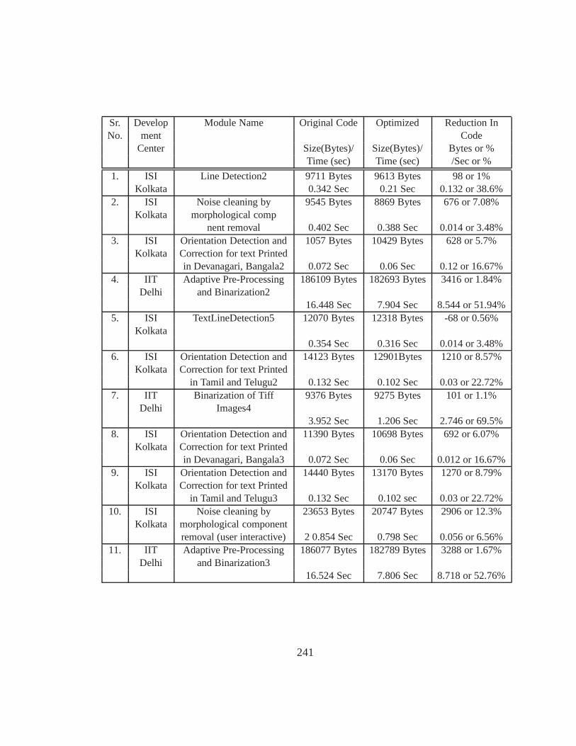
Sr. Develop Module Name Original Code Optimized Reduction InNo. ment Code
Center Size(Bytes)/ Size(Bytes)/ Bytes or %Time (sec) Time (sec) /Sec or %
1. ISI Line Detection2 9711 Bytes 9613 Bytes 98 or 1%Kolkata 0.342 Sec 0.21 Sec 0.132 or 38.6%
2. ISI Noise cleaning by 9545 Bytes 8869 Bytes 676 or 7.08%Kolkata morphological comp
nent removal 0.402 Sec 0.388 Sec 0.014 or 3.48%3. ISI Orientation Detection and 1057 Bytes 10429 Bytes 628 or 5.7%
Kolkata Correction for text Printedin Devanagari, Bangala2 0.072 Sec 0.06 Sec 0.12 or 16.67%
4. IIT Adaptive Pre-Processing 186109 Bytes 182693 Bytes 3416 or 1.84%Delhi and Binarization2
16.448 Sec 7.904 Sec 8.544 or 51.94%5. ISI TextLineDetection5 12070 Bytes 12318 Bytes -68 or 0.56%
Kolkata0.354 Sec 0.316 Sec 0.014 or 3.48%
6. ISI Orientation Detection and 14123 Bytes 12901Bytes 1210 or 8.57%Kolkata Correction for text Printed
in Tamil and Telugu2 0.132 Sec 0.102 Sec 0.03 or 22.72%7. IIT Binarization of Tiff 9376 Bytes 9275 Bytes 101 or 1.1%
Delhi Images43.952 Sec 1.206 Sec 2.746 or 69.5%
8. ISI Orientation Detection and 11390 Bytes 10698 Bytes 692 or 6.07%Kolkata Correction for text Printed
in Devanagari, Bangala3 0.072 Sec 0.06 Sec 0.012 or 16.67%9. ISI Orientation Detection and 14440 Bytes 13170 Bytes 1270 or 8.79%
Kolkata Correction for text Printedin Tamil and Telugu3 0.132 Sec 0.102 sec 0.03 or 22.72%
10. ISI Noise cleaning by 23653 Bytes 20747 Bytes 2906 or 12.3%Kolkata morphological component
removal (user interactive) 2 0.854 Sec 0.798 Sec 0.056 or 6.56%11. IIT Adaptive Pre-Processing 186077 Bytes 182789 Bytes 3288 or 1.67%
Delhi and Binarization316.524 Sec 7.806 Sec 8.718 or 52.76%
241
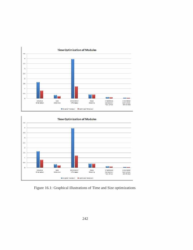
Figure 16.1: Graphical illustrations of Time and Size optimizations
242

Chapter 17
Development of Image Corpus andAnnotation
17.1 Background
Datasets are prerequisites for the development, evaluation, performance enhancement andbenchmarking of data driven document analysis systems. Lack of linguistic resources inthe form of annotated datasets has been one of the hurdles in building robust documentunderstanding systems for Indian languages. There is a pressing need for very large col-lections of training data if robust systems have to be built for Indian language documentunderstanding. Image data is to be labeled with corresponding information in order to makeuse of it for training. Annotation of document images is doneat different levels to be ableto make use of the data to the best. Block level annotation with text non-text distinction isdone. At text block, line and word level, corresponding textis aligned to the boundaries ofthe image component.
17.2 Objective
Preparation of image corpus for all the Indian languages of interest is one of the primaryobjective of this project. This corpus could enable extensive experimentation, training aswell as testing. It is aimed to have around 5000 pages of imagecorpus for each of theselanguages. Annotation of the scanned document images is also aimed by the project. Helpof particular language groups are seeked in identifying books and annotation. Project aimsto deliver a large corpus of annotated data in a structured form (in xml and/or traditionaldatabase). It has the following contents
243

1. Image scanned at multiple resolutions and processed.
2. Text corpus.
3. Bounding box of word with corresponding text.
4. Program interfaces (APIs) to make use of the corpus easily.
17.3 Annotation Process
In the first phase of this project, we designed and experimented with an annotation process.The process has to be highly similar for all languages. It should also scale to large numberof documents.
Image corpus is prepared with at most care. Preparation of image corpus is done bykeeping in mind that this will be primarily used for trainingand testing of OCRs in Indianlanguages. Scanning is done using a flat bed scanner. Then theimages are skew correctedand thresholded. Finally, these images are smoothened to reduce effect on content due tothresholding. These processes are done using a scanfix tool.
Once all the image processing is carried out page by page, they are stored in a structuredform in a directory with standardized naming conventions.
Annotation is done by labeling the boundaries of image components with correspondingcontent. Text content in the page is required for the annotation process. Document imageis segmented and then aligned with text. Segmentation and annotation at page level is donemanually. At line and word level, the annotation process is done as a semi automatic one,where only errors are corrected manually. Then the annotated data is stored in mysql baseddatabase and APIs are build to easily access the data. A diagram of the process is given inthe Figure 17.1.
The dataset is then stored in a well defined format. For each book, data is divided toground truth text, image corpus, annotation information and related meta data. The wholedata is stored as shown in Figure 17.2.
17.4 Development of Annotation Tools
A set of scripts and tools are designed and developed for various related tasks. They in-clude (i) Semi-automatic annotation tool (yaat) (ii) Font,code related converters (iii) imageprocessing algorithms for calibrating the scanfix for parameters like skew angle (iv) scripsfor creating image corpus from scanned images (v) Propagation of annotation (vi) image
244
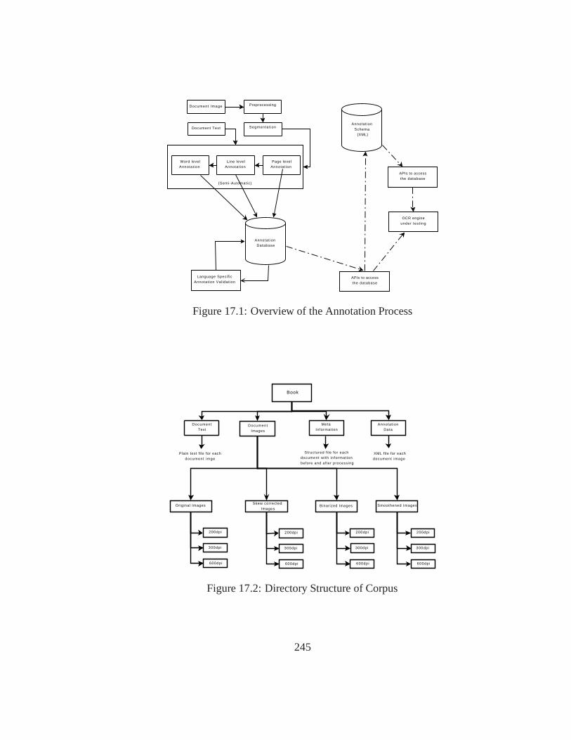
Document Image Preprocessing
Document Text Segmentat ion
Word levelAnnotation
Line levelAnnotation
Page levelAnnotation
(Semi-Automatic)
Annotation Database
Annotation Schema
(XML)
Language SpecificAnnotation Validation
APIs to access the database
APIs to access the database
OCR engine under test ing
Figure 17.1: Overview of the Annotation Process
Book
DocumentText
DocumentImages
Meta Information
Annotation Data
Plain text fi le for eachdocument imge
Structured fi le for each document with information before and after processing
XML file for eachdocument image
Original Images Skew corrected Images
Binarized Images Smoothened Images
200dpi
300dpi
600dpi
200dpi
300dpi
600dpi
200dpi
300dpi
600dpi
200dpi
300dpi
600dpi
Figure 17.2: Directory Structure of Corpus
245
processing plugins for the tool (vii) APIs for accessing theannotated data (viii) Tool forbrowsing the annotated data. These tools are developed in C/C++, perl or python.
Different tools are used at different levels of process. Scanfix is used for processing thescanned image. It deskews, thresholds and then smoothens the image. Information regard-ing the skew angle is stored as a part of the annotation metadata by reverse engineering thescanfix.
For doing the annotation at different hierarchical levels efficiently, special tool is devel-oped internally for the purpose. It takes in image and corresponding text file. Then allowsuser to manually segment and annotate at page level. Then, a semi automatic process isimplemented. Segmentation and annotation errors are corrected manually. It improves thespeed of the process extensively and allows user to correct any possible errors in typing andannotation.
Workshops are conducted in order to transfer the technologyto other language groups.APIs are prepared for efficient access of annotation data. For better and easier usage of
the annotation data, API is prepared as a shared library. It is made as a pluggable library.It can be used with any c++ program. Instructions to use the program and sample usagedetails are specified along with the API. Functional level documentation and user docu-mentation is provided for enhancing the user experience. API currently supports gettingboundaries of a random word, all words in a page and all words in a book.
17.5 Current Status of Annotation Process
The tables explain the current status of the image corpus across the languages includingthe number of books scanned, total pages in the corpus and number of images. Number ofimages is the total number of images including the differentresolution images, images atdifferent stages of processing etc. Table 17.2 gives a detail of total number of pages acrossdiffernt quality, present in the corpus. However, these quality estimates are subjective as ofnow.
Details of the annotation of the image corpus by the end of June can be seen in theTable 17.3.
17.6 Plans and Issues
The goal of 5000 page images in every language is mostly met. At an average we have 5000pages as of now. As a next step, more focus is given to the annotation process. Individuallanguage groups are given training on the process, tool etc.of the Annotation.
246
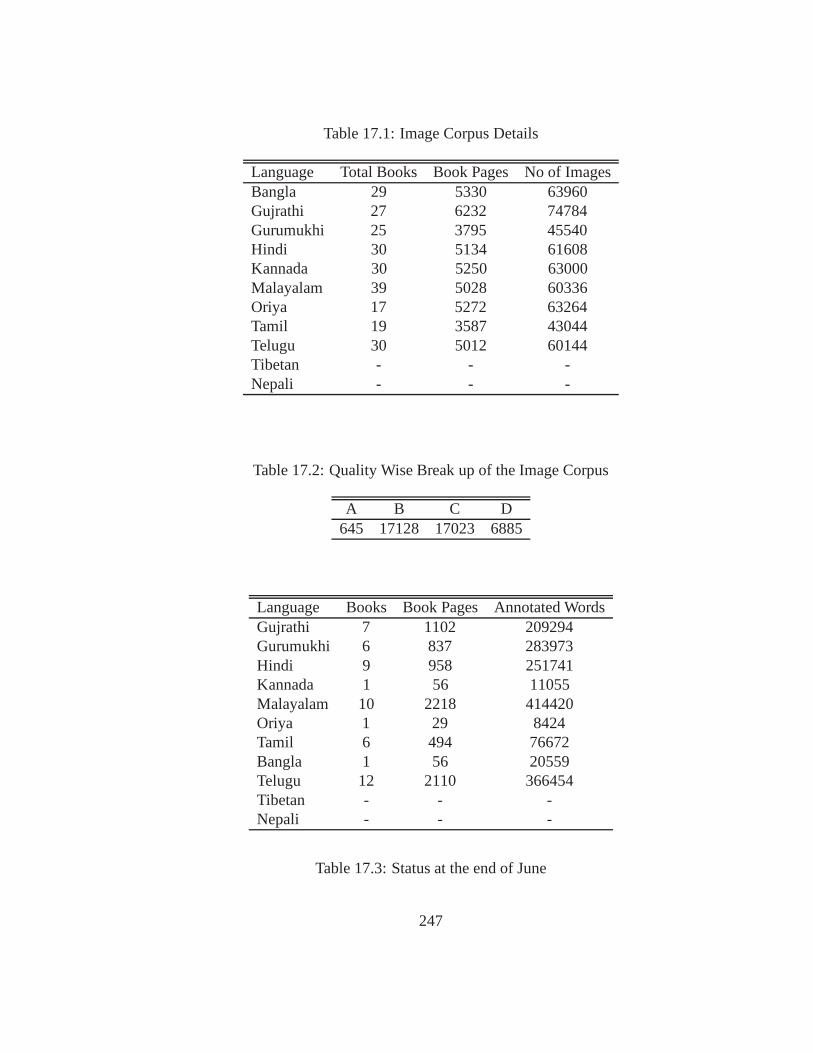
Table 17.1: Image Corpus Details
Language Total Books Book Pages No of ImagesBangla 29 5330 63960Gujrathi 27 6232 74784Gurumukhi 25 3795 45540Hindi 30 5134 61608Kannada 30 5250 63000Malayalam 39 5028 60336Oriya 17 5272 63264Tamil 19 3587 43044Telugu 30 5012 60144Tibetan - - -Nepali - - -
Table 17.2: Quality Wise Break up of the Image Corpus
A B C D645 17128 17023 6885
Language Books Book Pages Annotated WordsGujrathi 7 1102 209294Gurumukhi 6 837 283973Hindi 9 958 251741Kannada 1 56 11055Malayalam 10 2218 414420Oriya 1 29 8424Tamil 6 494 76672Bangla 1 56 20559Telugu 12 2110 366454Tibetan - - -Nepali - - -
Table 17.3: Status at the end of June
247

17.6.1 Challenges in Building of the corpus
Important challenges in annotation process can be enumerated as following.
1. The typed content used for the annotation should be of bestquality with 100 percentcorrectness.
2. Any missing words or lines in typed content will affect therate of annotation.
3. Mistakes below word level will affect the quality of the corpus generated.
17.6.2 Immediate Steps
1. Backing up of the precious resource prepared as part of theproject (more than a TerraBytes of Data) and duplicating it at other places.
2. Enabling individual language groups to contribute to theannotation.
3. Enabling individual language groups to use the data for OCR design.
4. Preparation of a more standard interfaces for correctionof any possible errors in thedatabase (till now, it was done through emails. It may move toa web site)
5. Version control of the corpus.
6. Content or structural Annotation of 5000 book pages by endof this year.
7. Refinement of quality classifications with the help of deeper insight from individuallanguage groups.
248
Chapter 18
Documentation
18.1 Introduction
Documentation is an important part of software engineering. Types of documentation in-clude:
1. Architecture/Design - Overview of software. Includes relations to an environment andconstruction principles to be used in design of software components.
2. Technical - Documentation of code, algorithms, interfaces, and APIs.3. End User - Manuals for the end-user, system administrators and support staff. This
manual will highlight some points that can help the engineers and the entire team tolearn and improve their efficiency and the performance of thesystem.
We propose to use Doxygen for Documentation of the source code.
18.2 Documentation of Code with Doxygen
Doxygen is a documentation system for C++, C, Java, Objective-C, Python, IDL (Corbaand Microsoft flavors) and to some extent PHP.
It can help you in the following ways:1. It can generate an on-line documentation browser (in HTML) and/or an off-line ref-
erence manual (in LaTeX) from a set of documented source files. There is also sup-port for generating output in RTF (MS-Word), PostScript, hyperlinked PDF, com-pressed HTML, and Unix man pages. The documentation is extracted directly fromthe sources, which makes it much easier to keep the documentation consistent withthe source code.
2. You can configure doxygen to extract the code structure from undocumented source
249
files. This is very useful to quickly find your way in large source distributions. Youcan also visualize the relations between the various elements by means of includedependency graphs, inheritance diagrams, and collaboration diagrams, which are allgenerated automatically.
Doxygen is developed under Linux and Mac OS X, but is set-up tobe highly portable. Asa result, it runs on most other Unix flavors as well. Furthermore, executables for Windowsare available.
18.2.1 Getting Started
The executable doxygen is the main program that parses the sources and generates thedocumentation. See section Doxygen usage for more detailedusage information.
The executable doxytag is only needed if you want to generatereferences to externaldocumentation (i.e. documentation that was generated by doxygen) for which you do nothave the sources. See section Doxytag usage for more detailed usage information.
Optionally, the executable doxywizard can be used, which isa graphical front-end forediting the configuration file that is used by doxygen and for running doxygen in a graphicalenvironment.
The following figure shows the relation between the tools andthe flow of informationbetween them (it looks complex but that’s only because it tries to be complete):
Step 1: Creating a configuration file
Doxygen uses a configuration file to determine all of its settings. Each project should getits own configuration file. A project can consist of a single source file, but can also be anentire source tree that is recursively scanned.
To simplify the creation of a configuration file, doxygen can create a template configu-ration file for you. To do this call doxygen from the command line with the -g option:
[geet@mercury report]\$doxygen -g <config-file>
where ¡config-file¿ is the name of the configuration file. If youomit the file name, a filenamed Doxyfile will be created. If a file with the name ¡config-file¿ already exists, doxygenwill rename it to ¡config-file¿.bak before generating the configuration template. If you use
250
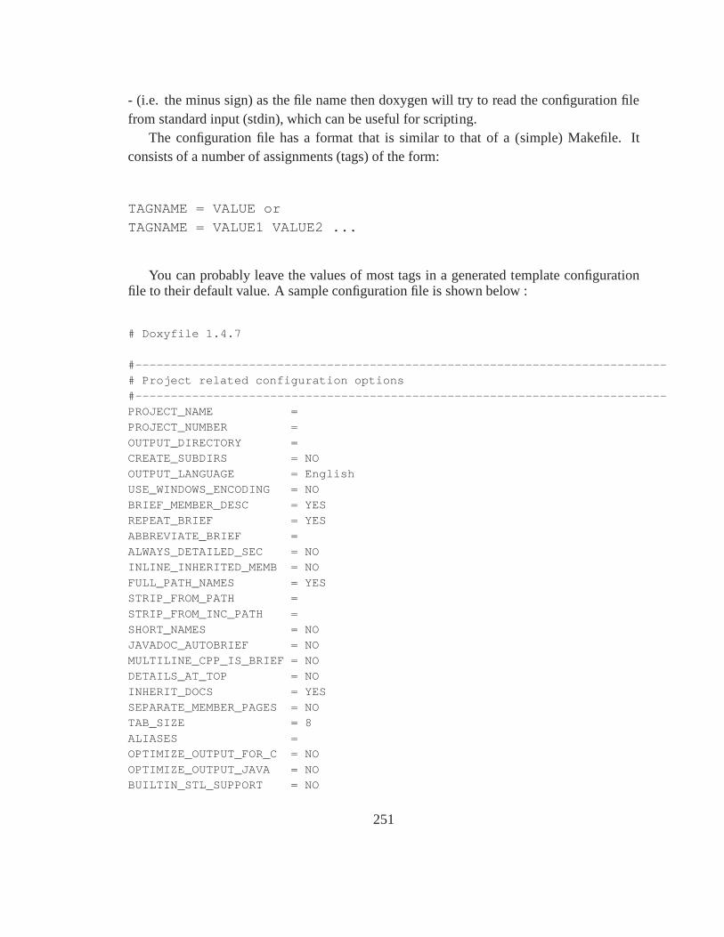
- (i.e. the minus sign) as the file name then doxygen will try toread the configuration filefrom standard input (stdin), which can be useful for scripting.
The configuration file has a format that is similar to that of a (simple) Makefile. Itconsists of a number of assignments (tags) of the form:
TAGNAME = VALUE or
TAGNAME = VALUE1 VALUE2 ...
You can probably leave the values of most tags in a generated template configurationfile to their default value. A sample configuration file is shown below :
# Doxyfile 1.4.7
#---------------------------------------------------------------------------# Project related configuration options
#---------------------------------------------------------------------------PROJECT_NAME =
PROJECT_NUMBER =
OUTPUT_DIRECTORY =CREATE_SUBDIRS = NO
OUTPUT_LANGUAGE = EnglishUSE_WINDOWS_ENCODING = NO
BRIEF_MEMBER_DESC = YESREPEAT_BRIEF = YES
ABBREVIATE_BRIEF =
ALWAYS_DETAILED_SEC = NOINLINE_INHERITED_MEMB = NO
FULL_PATH_NAMES = YESSTRIP_FROM_PATH =
STRIP_FROM_INC_PATH =
SHORT_NAMES = NOJAVADOC_AUTOBRIEF = NO
MULTILINE_CPP_IS_BRIEF = NODETAILS_AT_TOP = NO
INHERIT_DOCS = YES
SEPARATE_MEMBER_PAGES = NOTAB_SIZE = 8
ALIASES =OPTIMIZE_OUTPUT_FOR_C = NO
OPTIMIZE_OUTPUT_JAVA = NOBUILTIN_STL_SUPPORT = NO
251
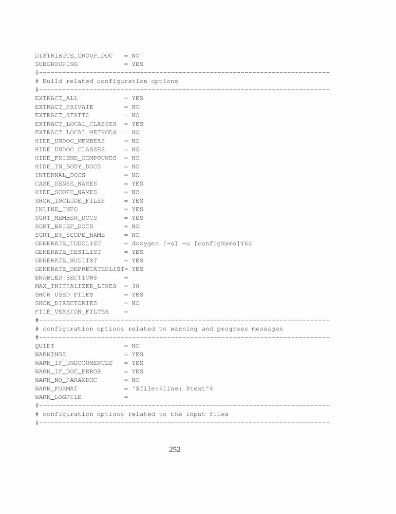
DISTRIBUTE_GROUP_DOC = NO
SUBGROUPING = YES#---------------------------------------------------------------------------
# Build related configuration options
#---------------------------------------------------------------------------EXTRACT_ALL = YES
EXTRACT_PRIVATE = NOEXTRACT_STATIC = NO
EXTRACT_LOCAL_CLASSES = YES
EXTRACT_LOCAL_METHODS = NOHIDE_UNDOC_MEMBERS = NO
HIDE_UNDOC_CLASSES = NOHIDE_FRIEND_COMPOUNDS = NO
HIDE_IN_BODY_DOCS = NOINTERNAL_DOCS = NO
CASE_SENSE_NAMES = YES
HIDE_SCOPE_NAMES = NOSHOW_INCLUDE_FILES = YES
INLINE_INFO = YESSORT_MEMBER_DOCS = YES
SORT_BRIEF_DOCS = NO
SORT_BY_SCOPE_NAME = NOGENERATE_TODOLIST = doxygen [-s] -u [configName]YES
GENERATE_TESTLIST = YESGENERATE_BUGLIST = YES
GENERATE_DEPRECATEDLIST= YES
ENABLED_SECTIONS =MAX_INITIALIZER_LINES = 30
SHOW_USED_FILES = YESSHOW_DIRECTORIES = NO
FILE_VERSION_FILTER =#---------------------------------------------------------------------------
# configuration options related to warning and progress messages
#---------------------------------------------------------------------------QUIET = NO
WARNINGS = YESWARN_IF_UNDOCUMENTED = YES
WARN_IF_DOC_ERROR = YES
WARN_NO_PARAMDOC = NOWARN_FORMAT = "$file:$line: $text"$
WARN_LOGFILE =#---------------------------------------------------------------------------
# configuration options related to the input files
#---------------------------------------------------------------------------
252

INPUT =
FILE_PATTERNS =RECURSIVE = NO
EXCLUDE =
EXCLUDE_SYMLINKS = NOEXCLUDE_PATTERNS =
EXAMPLE_PATH =EXAMPLE_PATTERNS =
EXAMPLE_RECURSIVE = NO
IMAGE_PATH =INPUT_FILTER =
FILTER_PATTERNS =FILTER_SOURCE_FILES = NO
#---------------------------------------------------------------------------# configuration options related to source browsing
#---------------------------------------------------------------------------
SOURCE_BROWSER = NOINLINE_SOURCES = NO
STRIP_CODE_COMMENTS = YESREFERENCED_BY_RELATION = YES
REFERENCES_RELATION = YES
REFERENCES_LINK_SOURCE = YESUSE_HTAGS = NO
VERBATIM_HEADERS = YES#---------------------------------------------------------------------------
# configuration options related to the alphabetical class index
#---------------------------------------------------------------------------ALPHABETICAL_INDEX = NO
COLS_IN_ALPHA_INDEX = 5IGNORE_PREFIX =
#---------------------------------------------------------------------------# configuration options related to the HTML output
#---------------------------------------------------------------------------
GENERATE_HTML = YESHTML_OUTPUT = html
HTML_FILE_EXTENSION = .htmlHTML_HEADER =
HTML_FOOTER =
HTML_STYLESHEET =HTML_ALIGN_MEMBERS = YES
GENERATE_HTMLHELP = NOCHM_FILE =
HHC_LOCATION =
GENERATE_CHI = NO
253
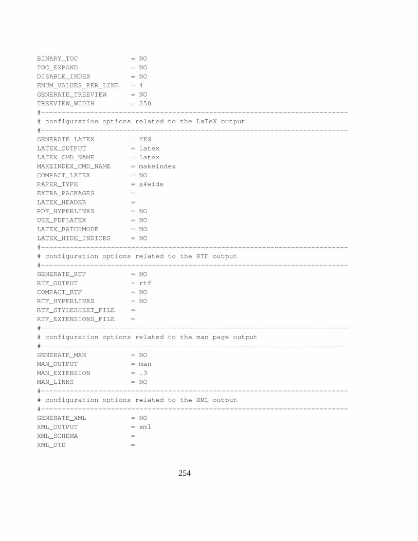
BINARY_TOC = NO
TOC_EXPAND = NODISABLE_INDEX = NO
ENUM_VALUES_PER_LINE = 4
GENERATE_TREEVIEW = NOTREEVIEW_WIDTH = 250
#---------------------------------------------------------------------------# configuration options related to the LaTeX output
#---------------------------------------------------------------------------
GENERATE_LATEX = YESLATEX_OUTPUT = latex
LATEX_CMD_NAME = latexMAKEINDEX_CMD_NAME = makeindex
COMPACT_LATEX = NOPAPER_TYPE = a4wide
EXTRA_PACKAGES =
LATEX_HEADER =PDF_HYPERLINKS = NO
USE_PDFLATEX = NOLATEX_BATCHMODE = NO
LATEX_HIDE_INDICES = NO
#---------------------------------------------------------------------------# configuration options related to the RTF output
#---------------------------------------------------------------------------GENERATE_RTF = NO
RTF_OUTPUT = rtf
COMPACT_RTF = NORTF_HYPERLINKS = NO
RTF_STYLESHEET_FILE =RTF_EXTENSIONS_FILE =
#---------------------------------------------------------------------------# configuration options related to the man page output
#---------------------------------------------------------------------------
GENERATE_MAN = NOMAN_OUTPUT = man
MAN_EXTENSION = .3MAN_LINKS = NO
#---------------------------------------------------------------------------
# configuration options related to the XML output#---------------------------------------------------------------------------
GENERATE_XML = NOXML_OUTPUT = xml
XML_SCHEMA =
XML_DTD =
254

XML_PROGRAMLISTING = YES
#---------------------------------------------------------------------------# configuration options for the AutoGen Definitions output
#---------------------------------------------------------------------------
GENERATE_AUTOGEN_DEF = NO#---------------------------------------------------------------------------
# configuration options related to the Perl module output#---------------------------------------------------------------------------
GENERATE_PERLMOD = NO
PERLMOD_LATEX = NOPERLMOD_PRETTY = YES
PERLMOD_MAKEVAR_PREFIX =#---------------------------------------------------------------------------
# Configuration options related to the preprocessor#---------------------------------------------------------------------------
ENABLE_PREPROCESSING = YES
MACRO_EXPANSION = NOEXPAND_ONLY_PREDEF = NO
SEARCH_INCLUDES = YESINCLUDE_PATH =
INCLUDE_FILE_PATTERNS =
PREDEFINED =EXPAND_AS_DEFINED =
SKIP_FUNCTION_MACROS = YES#---------------------------------------------------------------------------
# Configuration::additions related to external references
#---------------------------------------------------------------------------TAGFILES =
GENERATE_TAGFILE =ALLEXTERNALS = NO
EXTERNAL_GROUPS = YESPERL_PATH = /usr/bin/perl
#---------------------------------------------------------------------------
# Configuration options related to the dot tool#---------------------------------------------------------------------------
CLASS_DIAGRAMS = YESHIDE_UNDOC_RELATIONS = YES
HAVE_DOT = YES
CLASS_GRAPH = YESCOLLABORATION_GRAPH = YES
GROUP_GRAPHS = YESUML_LOOK = YES
TEMPLATE_RELATIONS = NO
INCLUDE_GRAPH = YES
255

INCLUDED_BY_GRAPH = YES
CALL_GRAPH = YESCALLER_GRAPH = YES
GRAPHICAL_HIERARCHY = YES
DIRECTORY_GRAPH = YESDOT_IMAGE_FORMAT = png
DOT_PATH =DOTFILE_DIRS =
MAX_DOT_GRAPH_WIDTH = 1024
MAX_DOT_GRAPH_HEIGHT = 1024MAX_DOT_GRAPH_DEPTH = 0
DOT_TRANSPARENT = NODOT_MULTI_TARGETS = NO
GENERATE_LEGEND = YESDOT_CLEANUP = YES
#---------------------------------------------------------------------------
# Configuration::additions related to the search engine#---------------------------------------------------------------------------
SEARCHENGINE = NO
If you do not wish to edit the config file with a text editor, you should have a look atdoxywizard, which is a GUI front-end that can create, read and write doxygen configurationfiles, and allows setting configuration options by entering them via dialogs.
If you have a larger project consisting of a source directoryor tree you should assignthe root directory or directories to the INPUT tag, and add one or more file patterns to theFILE PATTERNS tag (for instance⋆.cpp⋆.h). Only files that match one of the patternswill be parsed (if the patterns are omitted a list of source extensions is used). For recursiveparsing of a source tree you must set the RECURSIVE tag to YES.To further fine-tune thelist of files that is parsed the EXCLUDE and EXCLUDEPATTERNS tags can be used. Toomit all test directories from a source tree for instance, one could use:
EXCLUDE_PATTERNS = $\star$/test/$\star$
If you start using doxygen for an existing project (thus without any documentationthat doxygen is aware of), you can still get an idea of what thestructure is and how thedocumented result would look like. To do so, you must set the EXTRACT ALL tag inthe configuration file to YES. Then, doxygen will pretend everything in your sources isdocumented. Please note that as a consequence warnings about undocumented memberswill not be generated as long as EXTRACTALL is set to YES.
256
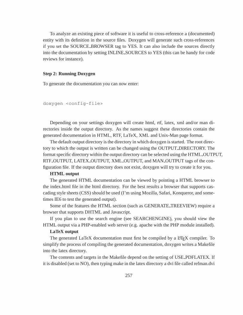
To analyze an existing piece of software it is useful to cross-reference a (documented)entity with its definition in the source files. Doxygen will generate such cross-referencesif you set the SOURCEBROWSER tag to YES. It can also include the sources directlyinto the documentation by setting INLINESOURCES to YES (this can be handy for codereviews for instance).
Step 2: Running Doxygen
To generate the documentation you can now enter:
doxygen <config-file>
Depending on your settings doxygen will create html, rtf, latex, xml and/or man di-rectories inside the output directory. As the names suggestthese directories contain thegenerated documentation in HTML, RTF, LaTeX, XML and Unix-Man page format.
The default output directory is the directory in which doxygen is started. The root direc-tory to which the output is written can be changed using the OUTPUT DIRECTORY. Theformat specific directory within the output directory can beselected using the HTMLOUTPUT,RTF OUTPUT, LATEX OUTPUT, XML OUTPUT, and MANOUTPUT tags of the con-figuration file. If the output directory does not exist, doxygen will try to create it for you.
HTML outputThe generated HTML documentation can be viewed by pointing aHTML browser to
the index.html file in the html directory. For the best results a browser that supports cas-cading style sheets (CSS) should be used (I’m using Mozilla,Safari, Konqueror, and some-times IE6 to test the generated output).
Some of the features the HTML section (such as GENERATETREEVIEW) require abrowser that supports DHTML and Javascript.
If you plan to use the search engine (see SEARCHENGINE), you should view theHTML output via a PHP-enabled web server (e.g. apache with the PHP module installed).
LaTeX outputThe generated LaTeX documentation must first be compiled by aLATEX compiler. To
simplify the process of compiling the generated documentation, doxygen writes a Makefileinto the latex directory.
The contents and targets in the Makefile depend on the settingof USE PDFLATEX. Ifit is disabled (set to NO), then typing make in the latex directory a dvi file called refman.dvi
257

will be generated. This file can then be viewed using xdvi or converted into a PostScriptfile refman.ps by typing make ps (this requires dvips).
To put 2 pages on one physical page use make ps2on1 instead. The resulting PostScriptfile can be send to a PostScript printer. If you do not have a PostScript printer, you can tryto use ghostscript to convert PostScript into something your printer understands.
Conversion to PDF is also possible if you have installed the ghostscript interpreter; justtype make pdf (or make pdf2on1).
To get the best results for PDF output you should set the PDFHYPERLINKS andUSE PDFLATEX tags to YES. In this case the Makefile will only contain a target to buildrefman.pdf directly.
RTF output
Doxygen combines the RTF output to a single file called refman.rtf. This file is opti-mized for importing into the Microsoft Word. Certain information is encoded using field.To show the actual value you need to select all (Edit - select all) and then toggle fields (rightclick and select the option from the drop down menu).
XML output
The XML output consists of a structured ”dump” of the information gathered by doxy-gen. Each compound (class/namespace/file/...) has its own XML file and there is also anindex file called index.xml.
A file called combine.xslt XSLT script is also generated and can be used to combine allXML files into a single file.
Doxygen also generates two XML schema files index.xsd (for the index file) and com-pound.xsd (for the compound files). This schema file describes the possible elements, theirattributes and how they are structured, i.e. it the describes the grammar of the XML filesand can be used for validation or to steer XSLT scripts.
In the addon/doxmlparser directory you can find a parser library for reading the XMLoutput produced by doxygen in an incremental way (see addon/doxmlparser/include/doxmlintf.hfor the interface of the library)
Man page output
The generated man pages can be viewed using the man program. You do need to makesure the man directory is in the man path (see the MANPATH environment variable). Notethat there are some limitations to the capabilities of the man page format, so some infor-mation (like class diagrams, cross references and formulas) will be lost.
258
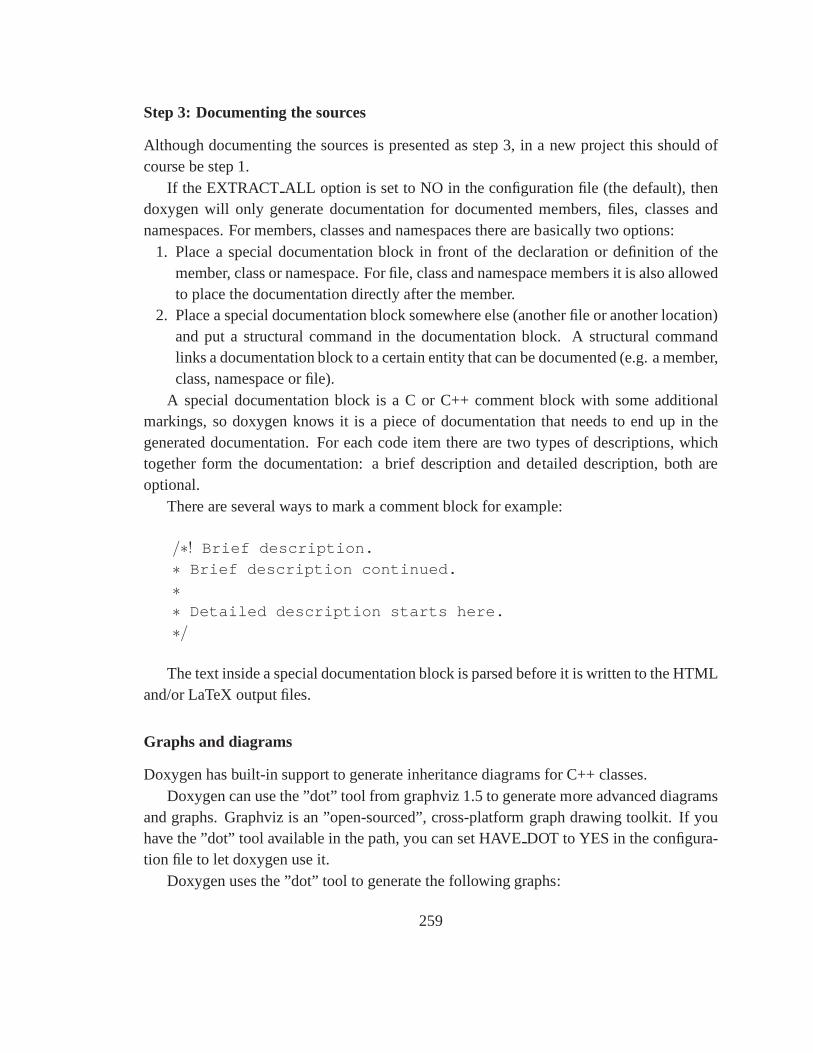
Step 3: Documenting the sources
Although documenting the sources is presented as step 3, in anew project this should ofcourse be step 1.
If the EXTRACT ALL option is set to NO in the configuration file (the default),thendoxygen will only generate documentation for documented members, files, classes andnamespaces. For members, classes and namespaces there are basically two options:
1. Place a special documentation block in front of the declaration or definition of themember, class or namespace. For file, class and namespace members it is also allowedto place the documentation directly after the member.
2. Place a special documentation block somewhere else (another file or another location)and put a structural command in the documentation block. A structural commandlinks a documentation block to a certain entity that can be documented (e.g. a member,class, namespace or file).
A special documentation block is a C or C++ comment block withsome additionalmarkings, so doxygen knows it is a piece of documentation that needs to end up in thegenerated documentation. For each code item there are two types of descriptions, whichtogether form the documentation: a brief description and detailed description, both areoptional.
There are several ways to mark a comment block for example:
/∗! Brief description.
∗ Brief description continued.
∗∗ Detailed description starts here.
∗/
The text inside a special documentation block is parsed before it is written to the HTMLand/or LaTeX output files.
Graphs and diagrams
Doxygen has built-in support to generate inheritance diagrams for C++ classes.Doxygen can use the ”dot” tool from graphviz 1.5 to generate more advanced diagrams
and graphs. Graphviz is an ”open-sourced”, cross-platformgraph drawing toolkit. If youhave the ”dot” tool available in the path, you can set HAVEDOT to YES in the configura-tion file to let doxygen use it.
Doxygen uses the ”dot” tool to generate the following graphs:
259
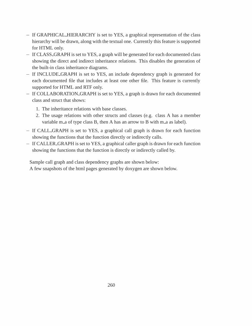
− If GRAPHICAL HIERARCHY is set to YES, a graphical representation of the classhierarchy will be drawn, along with the textual one. Currently this feature is supportedfor HTML only.
− If CLASS GRAPH is set to YES, a graph will be generated for each documented classshowing the direct and indirect inheritance relations. This disables the generation ofthe built-in class inheritance diagrams.
− If INCLUDE GRAPH is set to YES, an include dependency graph is generatedforeach documented file that includes at least one other file. This feature is currentlysupported for HTML and RTF only.
− If COLLABORATION GRAPH is set to YES, a graph is drawn for each documentedclass and struct that shows:
1. The inheritance relations with base classes.2. The usage relations with other structs and classes (e.g. class A has a member
variable ma of type class B, then A has an arrow to B with ma as label).
− If CALL GRAPH is set to YES, a graphical call graph is drawn for each functionshowing the functions that the function directly or indirectly calls.
− If CALLER GRAPH is set to YES, a graphical caller graph is drawn for eachfunctionshowing the functions that the function is directly or indirectly called by.
Sample call graph and class dependency graphs are shown below:A few snapshots of the html pages generated by doxygen are shown below.
260
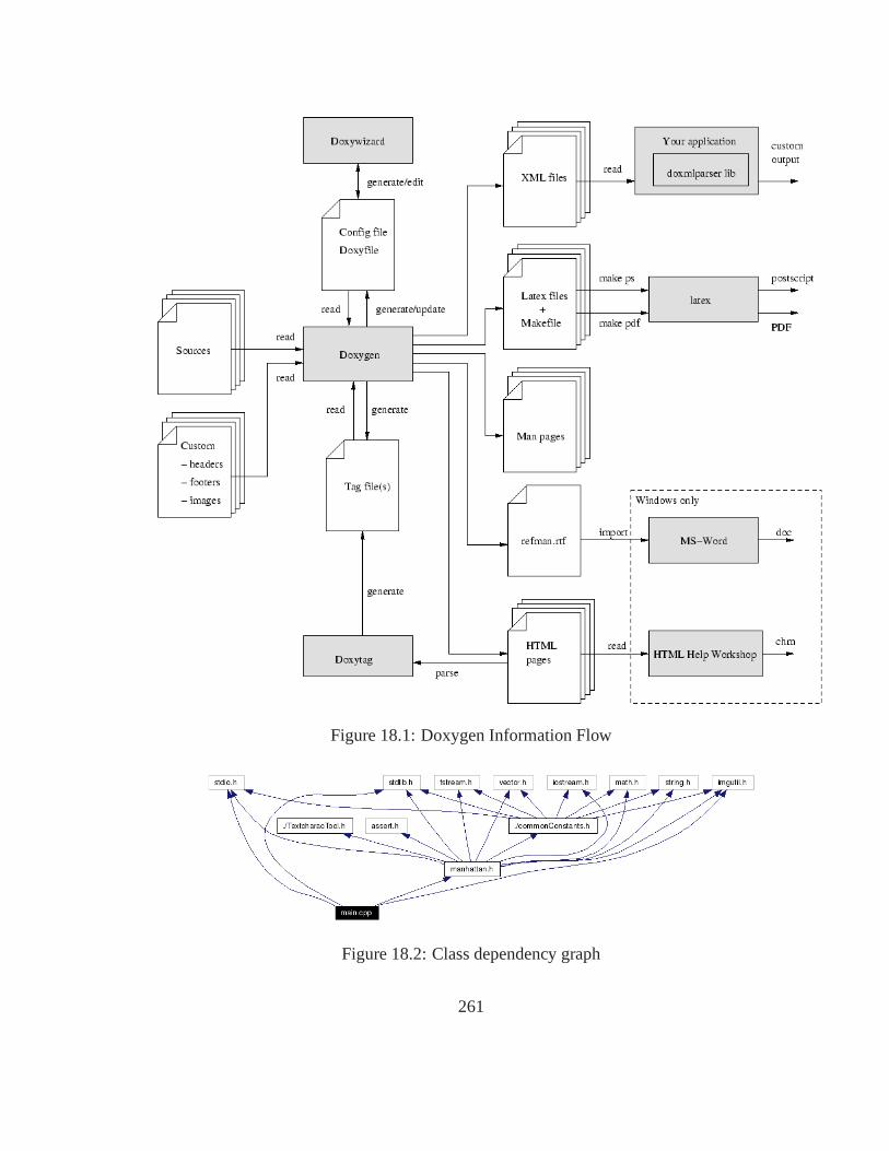
Figure 18.1: Doxygen Information Flow
Figure 18.2: Class dependency graph
261
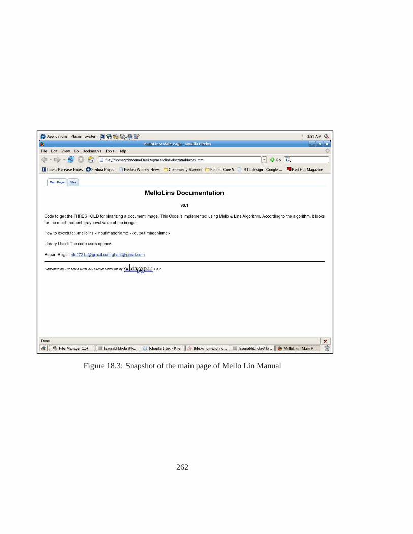
Figure 18.3: Snapshot of the main page of Mello Lin Manual
262
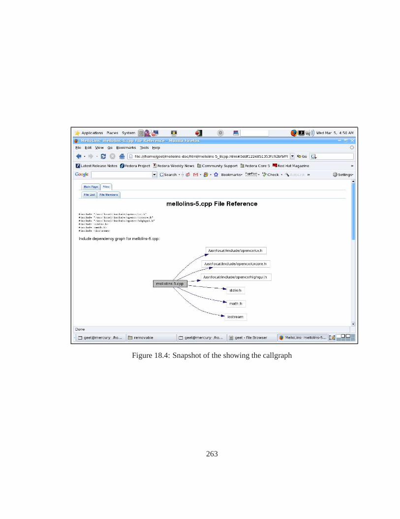
Figure 18.4: Snapshot of the showing the callgraph
263
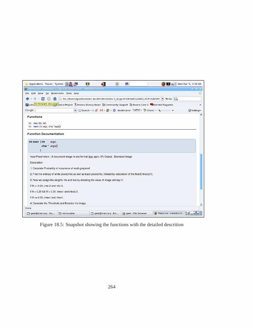
Figure 18.5: Snapshot showing the functions with the detailed descrition
264

Figure 18.6: Snapshot of the main page of Adaptive Thresholding and Noise RemovalManual
265
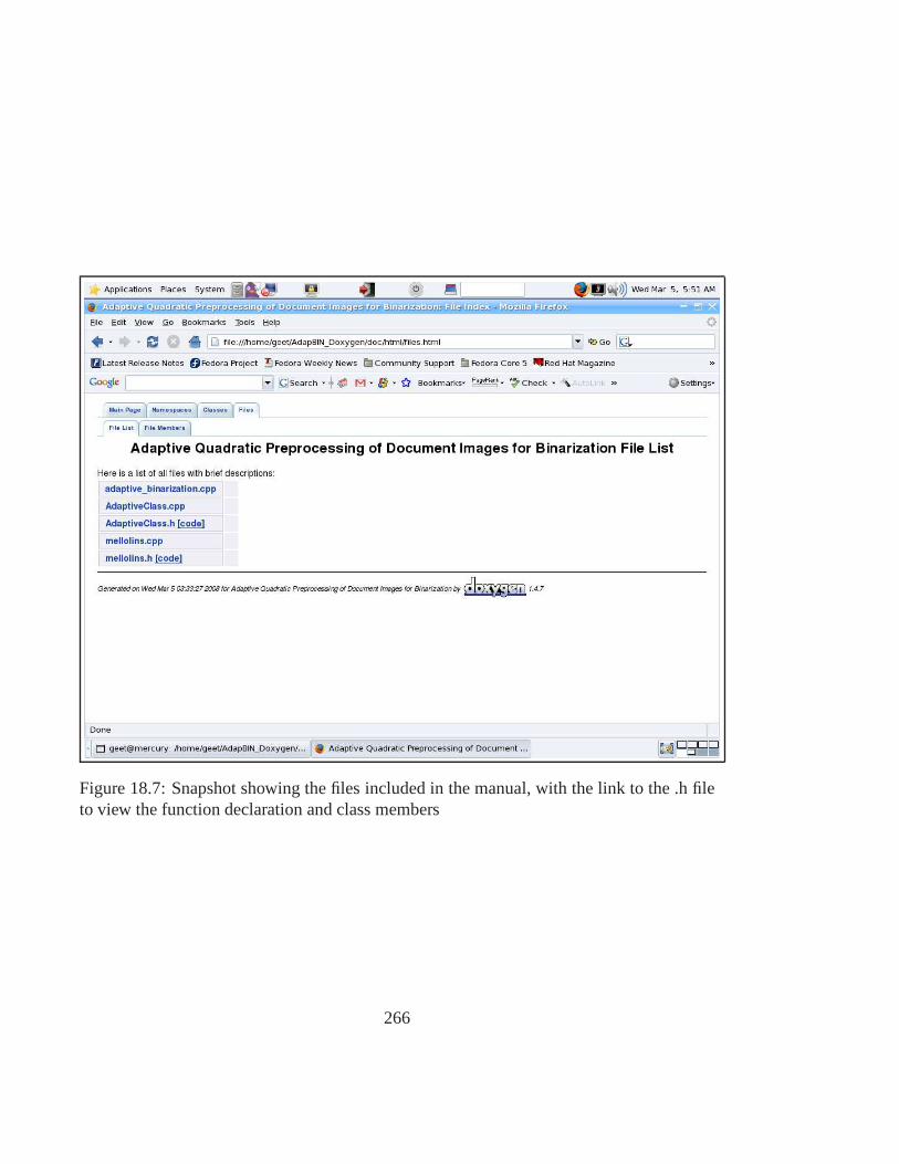
Figure 18.7: Snapshot showing the files included in the manual, with the link to the .h fileto view the function declaration and class members
266
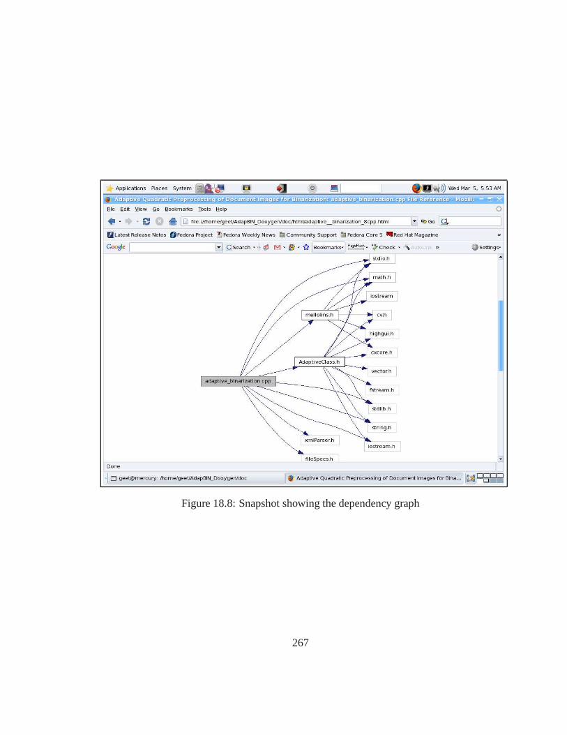
Figure 18.8: Snapshot showing the dependency graph
267
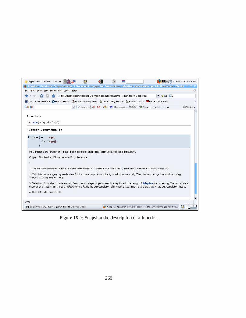
Figure 18.9: Snapshot the description of a function
268
References
[1] O. Kolak, W. Byrne, and P. Resnik, “A Generative Probabilistic OCR Model for NLPApplications,” inProc. of HLT-NAACL, (Edmonton), pp. 55 – 62, May-June 2003.
[2] V. Bansal and R. M. K. Sinha, “Integrating Knowledge Sources in Devnagri TextRecognition,”IEEE Transactions on Systems, Man, and Cybernetics - Part A:Systemsand Humans, vol. 30, pp. 500 – 505, July 2000.
[3] R. M. K. Sinha and H. N. Mahabala, “Machine recognition ofDevanagari script,”IEEE Trans. Syst. Man, Cybern. vol. SMC-9, pp. 435 – 441, 1979.
[4] OmniGlot: http://www.omniglot.com.
[5] S. Y. Mehta and J. Dholakia
[6] A. S. Ramamohan, “Gujarati Numeral Recognition using Wavelets and Neural Net-work,” in Proc. IICAI, 2005.
[7] S. R. M. Archit Yajnik, “Identification of Gujarati Characters Using Wavelets andNeural Networks,” inArtificial Intelligence and Soft Computing, 2006.
[8] A. N. J.Dholakia, Archit Yajnik, “Wavelet Feature BasedConfusion Character Setsfor Gujarati Script,” inICCIMA, 2007.
[9] G. Nagy, T. A. Nartker, and S. V. Rice, “Optical CharacterRecognition: An illus-trated guide to the frontier,” inProc. Document Recognition and Retrieval VII SPIE,vol. 3967, (San Jose, CA), pp. 58 – 69, Jan 2000.
[10] H. Baird, “The Skew Angle of Printed Documents,”In Proceedings of the ConferenceSociety of Photographic Scientists and Engineers, pp. 14 – 21, 1987.
[11] P. N. Gatos, B. and C. Chamas, “Skew Detection and Text Line Position Determi-nation in Digitized Documents,”Pattern Recognition, vol. 30(9), pp. 1505 – 1519,1997.
269
[12] F. J. Hinds, S. and D. D’ Amatos, “A Document skew detection method using run-lenth encoding and the Hough Transform,”In Proceedings of the 10th internationalConference on Pattern Recognition, pp. 464 – 468, 1990.
[13] R. R.C.Gonzalez,Digital image processing. 2 ed.
[14] N. Otsu, “A threshold selection method from gray level histograms,”IEEE Transac-tions on Systems Man and Cybernetics, vol. 9, pp. 62 – 66, Jan 1979.
[15] C. A. B. Mello and R. D. Lins,Image segmentation of historical documents. Mexico:Visual Mexico City, 2000.
[16] R. D. L. et al, “An Environment for Processing Images of Historical Documents,” inMicroprocessing and Microprogramming, North-Holland, pp. 111 – 121, 1995.
[17] R. M. H. I. T. P. Jaekyu Ha, “Recursive X-Y Cut using Bounding Boxes of ConnectedComponents,”Third International Conference on Document Analysis and Recogni-tion (ICDAR’95), vol. 2, 1995.
[18] L. O’Gorman, “The document spectrum for page layout analysis,” IEEE TPAMI,vol. 15, pp. 1162 – 1173, Nov 1993.
[19] C.-C. Chang and C.-J. Lin, “A library for support vectormachines.” Website.
[20] H. L. Yefeng Zheng and D. Doermann, “Machine printed text and handwriting iden-tification in noisy document images,” IEEE Trans. On PAMI.
[21] R. Z. Yuri Boykov, Olga Veksler, “Fast Approximate Energy Minimization via GraphCuts.,” IEEE Trans. On PAMI, vol. 11, pp. 1222 – 1239, march 2004.
[22] V. Kolmogorov and R. Zabih., “What energy functions can be minimized via graphcuts.,” IEEE Transactions on Pattern Analysis and Machine Intelligence, vol. 26(2),pp. 147 – 159, february 2004.
[23] R. G. Casey and D. R. Furgson, “Intelligent forms processing,” in IBM Syst. J, vol. 29,1990.
[24] S. Liang, M. Shridhar, and M. Ahmad, “Segmentation of touching characters inprinted document recognition,”Pattern Recognit, vol. 27, pp. 825 – 840, 1994.
[25] J. J. Hull, S. N. Srihari, and R. Choudhari, “An integrated algorithm for text recog-nition: Comparison with cascaded algorithm,”IEEE Trans Pattern Anal. MachineIntell. vol. PAMI-5, pp. 384 – 395, 1983.
270
[26] E. M. Riseman and A. R. Hanson, “A contextual post processing system for errorcorrection using binary n-grams,”IEEE Trans. Comput, vol. C-23, pp. 480 – 493,1974.
[27] R. M. K. Sinha, B. Prasada, G. Houle, and M. Sabourin, “Hybrid contextual textrecognition with string matching,”IEEE Trans. Pattern Anal Machine Intell, vol. 15,pp. 915 – 925, 1993.
[28] R. Shinghal, “A hybrid algorithm for contextual text recognition,”Pattern Recognit,vol. 16, pp. 261 – 267, 1983.
[29] S. N. Srihari, J. J. Hull, and R. Choudhari, “Integrating diverse knowledge sources intext recognition,”ACM Transactions on Office Information Systems, vol. 1, pp. 68 –87, Jan 1983.
[30] H. Takahashi, N. Itoh, T. Amano, and A. Yamashita, “A spelling correction methodand its application to an OCR system,”Pattern Recognit, vol. 23, pp. 363 – 377, 1990.
[31] T. K. Ho, J. J. Hull, and S. N. Srihari, “Decision combination in multiple classifiersystems,”IEEE Trans. Pattern Anal. Machine Intell, vol. 16, pp. 66 – 75, 1994.
[32] S. Kahan, T. Pavlidis, and H. S. Baird, “On the recognition of printed characters of anyfont and size,”IEEE Trans. Pattern Anal. Machine Intell. vol. PAMI-9, pp. 274 – 287,1987.
[33] V. Bansal and R. M. K. Sinha, “On integrating diverse knowledge sources in opticalreading of Devanagari script,” inProc. Int. Conf Information Systems Analysis andSynthesis (ISAS’96), (Orlando, FL), 1996.
[34] S. S. Marwah, S. K. Mullick, and R. M. K. Sinha, “Recognition of Devanagari charac-ters using a hierarchical binary decision tree classifier,”in IEEE Int. Conf. Syst. Man,Cybern, Oct 1994.
[35] R. M. K. Sinha, “Rule based contextual post-processingfor Devanagari text recogni-tion,” Pattern Recognit, vol. 20, pp. 475 – 485, 1987.
[36] J. C. Sant and S. K. Mullick, “Handwritten Devanagari script recognition usingCTNNSE algorithm,” inInt. Conf. Application of Information Technology South AsianLanguage, Feb 1994.
[37] I. K. Sethi and B. Chatterjee, “Machine recognition of hand printed Devanagari nu-merals,”J. Inst. Electron. Telecommun. Eng, vol. 22, pp. 532 – 535, 1976.
271
[38] B. B. Chaudhuri and U. Pal, “A complete printed Bangla OCR system,”PatternRecognit, vol. 31, no. 5, pp. 531 – 549, 1997.
[39] B. B. Chaudhuri and U. Pal, “An OCR system to read two Indian language scripts:Bangla and Devanagari,” inProc. 4th Int. Conf. Document Analysis and Recognition,pp. 1011 – 1015, 1997.
[40] S. J.Dholakia, A.Negi, “Zone Identification in PrintedGujarati Text,” inProc. ICDAR,2005.
[41] B. Vijayakumar and A. G. Ramakrishnan, “Machine Recognition of Printed KannadaText,” Document Analysis Systems V, Ed. D Lopresti, J Hu and R Kashi, pp. 37 – 48,2002.
[42] T. V. Ashwin and P. S. Shastry, “A font and size independent ocr system for printedkannada documents using support vector machines,” SADHANA, vol. 27 Part 1,pp. 35 – 58, Feb 2002.
[43] P. B. Pati and A. G. Ramakrishnan, “OCR in Indian Scripts: A Survey,” IETE Techni-cal Review, vol. 22, No. 3, pp. 217 – 227, May-June 2005.
[44] C.-W. Hsu and C.-J. Lin, “A comparison of methods for multiclass support vectormachines,” IEEE Trans. Neu. Net., vol. 13, pp. 415 – 425, 2002.
[45] B. T. Messmer and H. Bunke, “Efficient Subgraph Isomorphism Detection: A Decom-position Approach,” IEEE Trans. Knowl. Data Eng. 12(2), pp. 307 – 323, 2000.
[46] B. T. Messmer and H. Bunke, “A decision tree approach to graph and subgraph iso-morphism detection,” Pattern Recognition, vol. 32(12), 1999.
[47] K. Kukich, “Techniques for automatically correcting words in text,”ACM ComputingSurveys, vol. 24, pp. 377 – 439, December 1992.
[48] A. R. Hanson, E. M. Riseman, and E. G. Fisher, “Context inword recognition,”Pat-tern Recognition, vol. 8, pp. 33 – 45, 1976.
[49] R. M. K. Sinha and B. Prasada, “Visual text recognition through contextual process-ing,” Pattern Recognition, vol. 21, no. 5, pp. 463 – 479, 1988.
[50] A. Goshtasby and R. W. Ehrich, “Contextual word recognition using probabilisticrelaxation labeling,”Pattern Recognition, vol. 21, no. 5, pp. 455 – 462, 1988.
272
[51] M. A. Jones, G. A. Story, and B. W. Ballard, “Integratingmultiple knowledge sourcesin a Bayesian OCR post-processor,” inICDAR, (St Malo, France), 1991.
[52] J. C. Perez-Cortes, J.-C. Amengual, J. Arlandis, and R.Llobet, “Stochastic error-correcting parsing for OCR post-processing,” inICPR, (Barcelona, Spain), September2000.
[53] U. Pal, P. K. Kundu, and B. B. Chaudhuri, “OCR Error Correction of an InflectionalIndian Language Using Morphological Parsing,”Journal of Information Science andEngineering, vol. 16, pp. 903 – 922, 2000.
[54] K. Taghva and E. Stofsky, “OCRSpell: an interactive spelling correction system forOCR errors in text,”IJDAR, vol. 3, no. 3, pp. 125 – 137, 2001.
[55] T. Kanungo, P. Resnik, S. Mao, D. wan Kim, and Q. Zheng, “The bible, truth, andmultilingual optical character recognition.” in revision.
[56] D. Doermann, H. Ma, B. Karagol-Ayan, and D. W. Oard, “Translation lexicon acquisi-tion from bilingual dictionaries,” inNinth SPIE Symposium on Document Recognitionand Retrieval, (San Jose, CA), 2002.
[57] R. Frederking, “Summary of the midas session on han-dling multilingual speech, document images, and video ocr.”http://www.clis2.umd.edu/conferences/midas/papers/frederking.txt, 1999.
[58] C. M. Strohmaier, C. Ringsletter, K. U. Schulz, and S. Mihov, “Lexical Postcorrectionof OCR-Results,” inProc. ICDAR, 2003.
273