Robust Traffic Scene Recognition with a Limited Descriptor Length

Ivan SikiricMireo d.d.

Buzinski prilaz 32HR-10000 Zagreb, Croatiaivan.sikiric@mireo.hr

Karla Brkic, Josip Krapac, Sinisa SegvicUniversity of Zagreb

Faculty of Electrical Engineering and ComputingUnska 3, HR-10000 Zagreb, Croatia

karla.brkic@fer.hr, josip.krapac@fer.hr, sinisa.segvic@fer.hr

Abstract

In this paper we describe a novel image descriptor de-signed for classification of traffic scene images in fleet man-agement systems. The descriptor is computationally simpleand very compact (as short as 48 bytes). It is derived fromvariations of two well known image descriptors: GIST andspatial Fisher vectors, thus encoding both global and localimage features. Both GIST (being a global scene descrip-tor) and spatial Fisher vectors (that relies on local imagefeatures) are tuned to produce very short outputs (64 com-ponents), which are then concatenated. The output is fur-ther compressed by a lossy encoding scheme, without sac-rificing classification performance. The encoding schemeuses as little as 3 bits to encode each vector component.The descriptor is evaluated on the publicly available FM2dataset of traffic scene images. We demonstrate very goodclassification performance matching that of full-sized gen-eral purpose image descriptors.

1. IntroductionRecognizing visual scenes while limiting the descriptor

size is a challenging problem with potential use in manyscenarios involving thin clients with limited bandwidths.Examples include autonomous unmanned aerial vehicles[35], driver assistance systems [13], fleet management sys-tems [29], mobile robots in emergency response situations[30], etc. We are assuming a scenario in which the serveris interested in retrieving and storing the information aboutthe visual surroundings of one or multiple thin clients atregular time intervals for a prolonged period of time (rang-ing from a week to a year), as illustrated in Figure 1. Thisinformation is used for further processing, e.g. for cross-checking GPS data, obtaining a semantic analysis of thethin clients’ behavior such as ”the UAV height loss is cor-related to the presence of birds in the scene”, etc. In sucha scenario, working with the raw image data generated bythe thin clients is prohibitively expensive both in terms of

Server

analyzing the descriptors

Thin clients

limited processing capabilities

computing short scene descriptors

Limited bandwidth

periodically transmitting descriptors

Database

limited storage capacity

storing the descriptors

Figure 1: Our target application framework, where a num-ber of thin clients send information about their surroundingsto a server via limited bandwidth.

Figure 2: Examples of scene types of interest in fleet man-agement systems, from the FM2 dataset [29].

data transfer and in terms of storage. Hence, a reasonablestrategy is storing only the descriptors of the images, andmaking these descriptors as short as possible.

This work deals with visual scene representations usinga very limited descriptor size (512 bytes and less). We arespecifically motivated by fleet management systems, wherea central server tracks the locations of a fleet of vehicles atany given time. The vehicles are equipped with a range ofsensors measuring a number of vehicle properties, a GPSsensor and a camera. The central server generates variousreports consisting of e.g. routes traveled, total number ofmiles, fuel expenditure etc. One recurring problem in fleetmanagement systems is the GPS sensor precision. Due toerroneous GPS output, it is often very hard to accuratelyreconstruct the route the vehicle has traveled. GPS errorsare most common in specific and visually easily recogniz-able places such as tunnels, toll booths or under overpasses.Therefore, GPS ambiguity in fleet management systemscould be resolved by storing the camera image of the ve-

1

Figure 3: Ambiguous route reconstruction due to poor GPSprecision. GPS readings are marked with red asterisks. It isequally plausible that the vehicle travelled the highway (inorange) and the local road (in white).

hicle’s surroundings and using it as a cue for both the likelyGPS failure and the correct location, e.g. by discerning lo-cal roads from highways and identifying tunnels and over-passes (Figure 2). Using this information, ambiguous routessuch as the one in Figure 3 could be easily resolved. How-ever, typical volumes of information generated by the fleetof vehicles, often involving hundreds of vehicles sending ininformation every minute, make it implausible to transmitand store entire images. The scene information should bestored in a descriptor of a very small size that is still suffi-ciently discriminative.

In this paper, we propose an efficient and short imagedescriptor that offers the same discriminative performanceas its state-of-the-art counterparts that are one or more or-ders of magnitude longer. We achieve this by combiningthe GIST descriptor [26, 27] with bag-of-words-based spa-tial Fisher vectors [17]. While GIST is a global descrip-tor, spatial Fisher vectors aggregate local image features,and we aim to capture ”the best of both worlds”. We ad-dress the problem of descriptor length by proposing an effi-cient encoding method, allowing some loss of data accuracyand precision, but without affecting measurable classifica-tion performance.

Note that beside fleet management systems, our ap-proach could also be used to aid place recognition systems,especially in scenarios of limited bandwidth. For example,it could provide a prior information on the scene type. Thescene type could be used to partition the search space formatching scenes, thus making the search process faster.

2. Related workOur work is closely related to the following topics: (i)

generic image classification, (ii) short image descriptors,(iii) traffic scene understanding and fleet management sys-tems and (iv) learning invariant properties of places and in-

variant image features.

2.1. Image classification

Bosch et al. [4] categorize generic scene modeling meth-ods for classification as either low-level or semantic. Meth-ods categorized as low-level simply represent the image asa collection of low-level features (e.g. color histograms) inorder to reduce the dimensionality for classification. In con-trast, methods categorized as semantic can be thought of ashaving some kind of prior understanding of what is beingrepresented. Examples of semantic methods include seman-tic objects, where an object detector signals the presence orabsence of a certain object type in order to assign a labelto the image [22], bags of visual words [12, 5, 19], where aset of meaningful visual words is retrieved from the trainingdata and used to classify query images, the GIST descriptor[26, 27], where the scene is represented globally via a set offilter responses, etc.

Bags of visual words have proven to be very successfulin the problem of image classification with a large numberof classes, as seen e.g. on the Pascal VOC dataset [11]. Anumber of extensions and modifications of the original bagsof visual words have been proposed [8], including locality-constrained linear coding (LLC) [34] and spatial Fisher vec-tors (SFV) [17].

2.2. Traffic scene understanding

In traffic scene analysis, most researchers devise meth-ods that are closely tailored to particular applications, giventhe constrained nature of the problem. Depending on thetarget application, methods range from scene segmentationand understanding at a pixel level [10] to generic sceneryclassification [32], or image-based localization [15].

Tang and Breckon [32] propose a method for road envi-ronment classification from images based on a set of colorand texture-based features extracted at predefined regionsof interest. They manually define the regions of interestto correspond to a sample of the road (in the center of theimage), the part of the road where it is the widest (at thebottom of the image), and the environment at the left sideof the road. Two classification problems are considered:either classifying images as off-road or on-road or a morefine-grained classification into off-road, urban scenery, ma-jor road and multilane motorway images. The work of Tangand Breckon is extended in [24], where only Gabor featuresare used, and the system is implemented using dedicatedhardware.

2.3. Short image descriptors

The volume of research on short image descriptors is rel-atively modest. Bergamo et al. have recently introduced Pi-CoDes [3] and mc (meta-class) [2] descriptors, which pro-duce very short image representations for the purpose of ef-

ficient image indexing in large image databases. Althoughvery good classification performance can be obtained, pro-ducing such descriptors is computationally very intensive,which makes them unsuitable for our thin client scenario.

Sikiric et al. [29] investigate the use of a number of state-of-the-art descriptors in the problem of traffic scene classi-fication, with an emphasis on the descriptor length. Theydescribe simple ways to tune each of the considered meth-ods to produce very short descriptors (as short as 64 floatingpoint numbers) while still retaining very good classificationperformance. Their findings show that GIST and spatialFisher vectors offer the best performance among the testeddescriptors when the goal is to minimize the feature vectorlength.

2.4. Visual scene understanding

Visual place recognition is of special interest in the prob-lem of simultaneous localization and mapping (SLAM) thatis actively researched in robotics [9, 23, 28]. Milford andWyeth [23] propose SeqSLAM, a SLAM algorithm thatuses full images instead of features such as SIFT [21]or SURF [1], matches image sequences instead of singleimages, and uses local contrast enhancement in the im-age distance matrix with the idea of reinforcing local in-stead of global match optimums. Input images are re-duced to a very small size (e.g. 64 × 32 pixels) and patch-normalized. Sunderhauf et al. [31] apply SeqSLAM on fourvideo sequences of a 728 km journey, one for each sea-son of the year. They report very good performance forsequences longer than 10 seconds, and a significant perfor-mance drop for mild viewpoint changes. The problem ofviewpoint variance is addressed in SMART, a SeqSLAM-inspired algorithm proposed by Pepperell et al. [28], by us-ing variable offset image matching. SMART offers severalother improvements over SeqSLAM such as sky blacken-ing. Sunderhauf and Protzel [31] introduce a descriptor forSLAM, called BRIEF-Gist, based on the BRIEF image de-scriptor [6], comparable to the popular FAB-Map [9], butmuch more computationally efficient.

2.5. Our contributions

In this paper, we build on the work of Sikiric et al. [29],who have found that GIST and spatial Fisher vectors per-form best in traffic scene classification when limiting thedescriptor length. We propose a way of combining thesetwo descriptors and efficiently encoding them in order toobtain a short scene representation that captures both localand global image structure.

Given the constrained nature of our target applicationthat involves a fleet management system serving a largenumber of vehicles with low processing power and lim-ited bandwidth, we do not consider processing-intensiveapproaches such as PiCoDeS [3] and mc (meta-class) [2].

Although SeqSLAM and SMART could be suitable in ourtarget scenario, we do not consider them because of theirreliance on scaled-down images. When scaled-down withthe default parameters of SeqSLAM/SMART, each imageamounts to about 6 kilobytes of data, and our goal is trans-mitting the descriptors of the size of 512 bytes and less. Forsimilar reasons, we do not consider BRIEF-Gist, as withbest-performing parameters it produces around 3 kilobytesof data per image.

We now briefly review the GIST image descriptor andspatial Fisher vectors and proceed to describe our method.

3. The GIST image descriptor

The GIST image descriptor [26, 27] is a global scene de-scriptor that provides a rough representation of the scenestructure by coarsely representing the distribution of orien-tations and scales in the scene. The descriptor is built byconvolving the input image with a number of Gabor filtersof varying scales and orientations. Each of the response im-ages is then divided into a regular grid of regions, and theresponses in each region are averaged. The final GIST de-scriptor is the concatenation of all the averaged responses.GIST is a compact representation that is very fast to com-pute [25], making it suitable for our target application sce-nario.

In [29], GIST is shown to be highly discriminative intraffic scene classification even when its size is reducedfrom 512 to 64 components. The reduction in size isachieved by using a grid of 2× 2 regions instead of the de-fault 4× 4, as well as using 4 orientations per scale insteadof the default 8.

4. Spatial Fisher vectors

Spatial Fisher vectors [17] are an extension of the well-known bag of visual words [12, 5, 19] descriptor. In bagsof visual words, each image is represented as an occurrencehistogram of a series of characteristic visual words. The vi-sual words used for building the histogram comprise the so-called visual vocabulary that is learned from a set of train-ing images. To build the vocabulary, a number of patches isextracted from each image, either through the use of an in-terest point detector or through dense sampling. Each patchis represented with a patch descriptor, e.g. SIFT [21]. Thedescriptors of the collected patches from all images are thenclustered intoK clusters, and cluster centroids represent vi-sual words constituting a K-word vocabulary. Given an im-age to be represented, the bag-of-visual-words descriptor isbuilt by extracting image patches and their descriptors fromthe image in the same manner as in the training process,finding the visual words that are nearest to the extractedpatches and building the histogram of the numbers of oc-currences of all the words in the visual vocabulary.

A weakness of the classical bags of visual words is thatthe representation does not retain any information about thespatial layout of the image. This problem is addressed inspatial Fisher vectors [17], where the spatial mean and vari-ance of the image regions associated with individual visualwords are encoded in the descriptors. The encoding is basedon the Fisher kernel framework and Gaussian mixture mod-els, used to represent appearance and spatial layout. Thepositions of the patches that are assigned to a visual wordare modeled using a Gaussian mixture model, so their spa-tial layout can be coded using one spatial Fisher vector pervisual word. Additionally, Fisher kernels are also used toencode the appearance of the features, reframing the origi-nal bag of visual words descriptors as Fisher vector repre-sentations for a simple multinomial probabilistic model. Ithas been shown [17] that spatial Fisher vectors can achieveequal performance as the original bags of visual words us-ing a smaller visual vocabulary, due to a more precise en-coding of the appearance information. Hence, the computa-tional cost of building a spatial Fisher vector representationis lower than for the classical bags of visual words and therepresentation itself is shorter, making spatial Fisher vectorsespecially suitable for our thin client with a limited band-width scenario.

5. Our methodThe GIST descriptor is designed for scene recognition,

and focuses of global image features while ignoring thesmall details in the scene. The spatial Fisher vectors de-scriptor is intended for general-purpose classification, andrelies only on local image features. This distinction inthe level of captured details is reflected on the classifica-tion performance of each descriptor in the context of traf-fic scenes, as shown e.g. in [29], where the GIST descrip-tor performs poorly on classes overpass and traffic, whilethe spatial Fisher vectors perform poorly on classes roadand toll booth. Recognition of overpasses and dense traf-fic in the scene is heavily dependent on modeling local fea-tures, while recognizing roads and toll booths is easier usingglobal scene models.

Intuitively, by using a simple concatenation of the GISTdescriptors and the spatial Fisher vectors we would captureboth the global and local image features, and therefore im-prove the overall classification performance. Additionally,we expect that by combining a GIST feature vector of lengthK and a spatial Fisher vector of lengthK, we might get bet-ter classification performance than by using either GIST ofspatial Fisher vectors of length 2K. Therefore, as a first stepin building a short and descriptive scene representation wepropose to concatenate the GIST and the spatial Fisher vec-tor descriptor of a scene into a single vector, as illustratedat the top of Figure 4. Each component is then normal-ized to have zero mean and unit variance, by subtracting the

GIST Spatial Fisher vector

Feature

vector

encoding

N(K1+K2) bits

N << 64

K1 64-bit numbers K2 64-bit numbers

Zero-mean

and unit-

variance

norm.

Figure 4: Our method: after obtaining shortened GIST andspatial Fisher vectors descriptors (of lengthsK1 andK2, re-spectively), their concatenation is normalized to zero mean,unit variance. Each component of the result is then en-coded using only N bits, so the total size of the output isN(K1 +K2) bits.

13.6%

*

+

x

*

+

x

inlier

sample

Bins: 1 2 3 4 5 6 7 8

outlier

sample

inlier sample

Figure 5: The encoding scheme for N = 3 bits and theinterval width of w = 4σ. The closed interval [−4σ, 4σ]is split into 23 = 8 equally wide bins. Value mapping isillustrated for three samples (orange, red and blue). Notethat the values outside the interval (the blue asterisk) aremapped to the nearest bin.

mean and dividing by variance, which are calculated fromthe training dataset.

To additionally reduce the memory footprint of the im-age feature vectors (and therefore also the bandwidth con-sumption), we propose a non-standard feature vector repre-sentation. The standard and straightforward representationof an image feature vector is an array of floating point num-bers of single or double precision, which uses 4 or 8 bytesper vector component, respectively. Our goal is to reducethe memory consumption to a maximum of 1 byte per com-ponent.

Instead of trying to encode the sign, exponent and man-tissa parts of a floating point number in 8 bits or less, we en-code each vector component in a fixed point representation,thus losing some accuracy and precision. More precisely, toencode a vector component using only N bits, we first mapits value to a closed interval [L,R], which is split into 2N

discrete bins. The index of a bin the value falls into is theencoded value of the component. Mapping into an interval

(a) highway (b) road (c) tunnel (d) tunnel exit

(e) settlement (f) overpass (g) toll booth (h) dense traffic

Figure 6: Examples of classes from the FM2 dataset

is done in such a way that a value outside the interval is setto the appropriate upper or lower interval limit, while othervalues remain unchanged. An illustration of this process isshown in Figure 5. The illustrated example assumes normaldata distribution, with zero mean. The width of the map-ping interval is set to include 4 standard deviations fromthe mean, thus including almost all observable values. Thisinterval is split into 23 = 8 equally wide bins, and the in-dex of the bin serves as the encoded value. If a value fallsoutside of the mapping interval, it is assigned to its nearestbin. So in this example, each component can be encodedusing only 3 bits. Decoding process is straightforward, wesimply replace each bin index with the coordinate of the bincenter. In the example in Figure 5 the decoded values forthe orange, red and blue samples would be −3.5σ, −3.5σand 1.5σ, respectively. Using a simple experimental setupwe can easily find the most appropriate interval width andnumber of bins for a given dataset and feature vector length.

6. ExperimentsTo experimentally validate the proposed descriptor, we

evaluate it on a dataset of traffic scenes while varying theparameters of the underlying GIST and spatial Fisher vectordescriptors, as well as the parameters of the feature vectorencoding. We now give more details on the dataset we used,describe our experimental setup, and present the results.

6.1. The FM2 dataset

The FM2 dataset [29] is a dataset of road scenes con-taining 6237 images categorized into eight classes: high-way, road, tunnel, tunnel exit, settlement, overpass, tollbooth and dense traffic. The images were recorded on roadsin Europe via a cellphone camera mounted inside a vehi-

Class label Imageshighway 4337road 516tunnel 601tunnel exit 64settlement 464overpass 86toll booth 75dense traffic 94

Table 1: Image distributions per class, the FM2 dataset.

cle, mainly at daytime and during sunny weather, usinga fairly constant viewpoint. The class labels are specifi-cally intended to be useful in a fleet management scenario,i.e. cover possible situations in which the loss of GPS pre-cision, traffic jams and slowdowns are likely. Example im-ages of all classes in the dataset are shown in Figure 2. Theclass balance is skewed in favor of highway images, as il-lustrated in Table 1.

The FM2 dataset comes with a publicly available pre-made train/validation/test splits, a 25/25/50 split for eachclass. In our experiments we use these splits to ensure com-parability of our results with previous work [29].

We note one weakness of the FM2 dataset labeling: onlyone class label is assigned per image, although there are im-ages that could be assigned to multiple classes. Examplesinclude e.g. toll booths and overpasses on a highway, densetraffic in a settlement etc. In this work, we retain the originalclass labels to remain comparable to [29]; however, assign-ing multiple labels to a single image should be consideredin future work.

6.2. Experimental setup

To evaluate the classification performance of the pro-posed descriptor combination, we use the method proposedin [29] to obtain GIST feature vectors and the spatial Fishervectors of lengths 64 and 128. From now on, we refer tothe spatial Fisher vectors of lengths 64, 128, etc. as SFV64and SFV128, etc. Similarly for GIST, we refer to the GISTdescriptors of lengths 64, 128, etc. as GIST64, GIST128,etc.

We measure the classification performance of threedifferent descriptor concatenations: GIST64+SFV64,GIST64+SFV128 and GIST128+SFV64. The classificationis performed with SVM (RBF kernel) and Random forestclassifiers, and we use mAP (mean of per-class average pre-cision) as a measure of performance. We will now describeeach experimental component in more detail.

6.2.1 The descriptors

For spatial Fisher vectors we use the dense SIFT imple-mentation from the VLFeat library [33] as a patch de-scriptor. The code for producing the spatial Fisher vectorsthemselves is based on code of Krapac et al. [17]. TheGaussian mixture model parameters are learned using theexpectation-maximization algorithm, and the diagonal ap-proximation of covariance matrix is used both for local de-scriptors and position features. We use the first 6 principalcomponents of the SIFT descriptors, and only one Gaussianper visual word, which means we use K visual words toobtain a vector of length 16K.

For the GIST descriptor we use the MATLAB implemen-tation provided by the authors [26, 27]. The implementationwas modified to reduce the grid size to 2 × 2 in order toproduce the 128-dimensional GIST descriptors. By furtherreducing the number of orientations per scale from 8 to 4,we obtain the 64-dimensional GIST descriptors.

6.2.2 The classification

As a preprocessing step for SVM classification, we trans-form all the feature vectors to zero mean and unit variance.The classification is then performed using the LibSVM li-brary [7], using the RBF kernel. For Random forest classi-fication we employ the code of Liaw et al. [20].

We use the default train/validation/test splits of the FM2dataset (25/25/50 split for each class). The classifier istrained on the training set, while the validation set is used tooptimize the parameters. Finally, the classifier is trained onthe union of training and validation sets using the optimizedparameters, and the final score is evaluated on the test set.In each step the mean average precision (mAP) is used as aperformance measure.

6.2.3 Feature vector encoding

We will now describe the experimental setup used toexplore the proposed memory-efficient vector encodingscheme. Let us briefly review the method: for each vectorcomponent, its value is mapped to a closed interval [L,R],which is split into 2N bins, thus encoding each componentusing only N bits. Values outside the interval are mappedto the nearest bin. Since we got very good results usinga GIST64+SFV64 concatenation with SVM classifier, wechoose this combination as our baseline. These feature vec-tors were transformed to have zero mean and unit variance,so the appropriate interval is of the form [−w,+w]. Bysetting the upper limit of the interval to three standard de-viations (w = 3), most of the observed values would beincluded in it (even without assuming normal distribution).However, the extreme values (falling outside of range ofthree standard deviations) could prove to be beneficial insuccessful class discrimination. To explore this, we run theexperiments with w set to 3, 3.5, 4, 4.5 and 5. We split theseintervals into 2N bins, with N set to 1, 2, 3, 4 and 8. Forsimplicity, we use the bins of equal size. We measure theclassification performance using the same instance of SVMclassifier which produced the optimal results for the unen-coded (full-size) GIST64+SFV64 combination. The vectorsfrom the testing dataset split are encoded and then decoded(thus introducing errors), and the classification performanceis then measured.

6.3. Experimental results

Classification results for the concatenated descriptors arepresented in Table 2 for the SVM classifier, and in Table 3for Random forest. The original results for the plain SFVand GIST descriptors from [29] are presented for conve-nience. There are several things we can note. Firstly, ourcombined descriptor GIST64+SFV64 indeed outperformsboth plain GIST128 and SFV128 descriptors, in case ofboth SVM and Random forest classifiers. In fact, better per-formance is only achieved using the spatial Fisher vectors oflength 2656 with an SVM classifier. We can also see that theSVM shows much better performance than the Random for-est classifier for all three combinations of our descriptors.Next, we note that slightly better performance is achievedwith GIST64+SFV128 than with GIST128+SFV64 descrip-tor. This implies that we should put more emphasis on localimage features to enable optimal class discrimination.

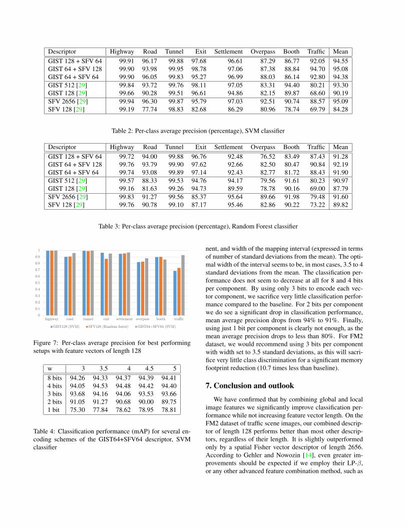
Graphical display of per-class performance for the best-performing setups with lengths of 128 is shown in Figure 7.The graph implies that the class traffic, containing imagesof dense traffic is the one that most benefits from combiningglobal and local image features.

The results of our feature vector encoding experimentsare shown in Table 4. The table shows dependency of meanaverage precision on two factors: number of bits per compo-

Descriptor Highway Road Tunnel Exit Settlement Overpass Booth Traffic MeanGIST 128 + SFV 64 99.91 96.17 99.88 97.68 96.61 87.29 86.77 92.05 94.55GIST 64 + SFV 128 99.90 93.98 99.95 98.78 97.06 87.38 88.84 94.70 95.08GIST 64 + SFV 64 99.90 96.05 99.83 95.27 96.99 88.03 86.14 92.80 94.38GIST 512 [29] 99.84 93.72 99.76 98.11 97.05 83.31 94.40 80.21 93.30GIST 128 [29] 99.66 90.28 99.51 96.61 94.86 82.15 89.87 68.60 90.19SFV 2656 [29] 99.94 96.30 99.87 95.79 97.03 92.51 90.74 88.57 95.09SFV 128 [29] 99.19 77.74 98.83 82.68 86.29 80.96 78.74 69.79 84.28

Table 2: Per-class average precision (percentage), SVM classifier

Descriptor Highway Road Tunnel Exit Settlement Overpass Booth Traffic MeanGIST 128 + SFV 64 99.72 94.00 99.88 96.76 92.48 76.52 83.49 87.43 91.28GIST 64 + SFV 128 99.76 93.79 99.90 97.62 92.66 82.50 80.47 90.84 92.19GIST 64 + SFV 64 99.74 93.08 99.89 97.14 92.43 82.77 81.72 88.43 91.90GIST 512 [29] 99.57 88.33 99.53 94.76 94.17 79.56 91.61 80.23 90.97GIST 128 [29] 99.16 81.63 99.26 94.73 89.59 78.78 90.16 69.00 87.79SFV 2656 [29] 99.83 91.27 99.56 85.37 95.64 89.66 91.98 79.48 91.60SFV 128 [29] 99.76 90.78 99.10 87.17 95.46 82.86 90.22 73.22 89.82

Table 3: Per-class average precision (percentage), Random Forest classifier

0

0.1

0.2

0.3

0.4

0.5

0.6

0.7

0.8

0.9

1

highway road tunnel exit settlement overpass booth traffic

GIST128 (SVM) SFV128 (Random forest) GIST64+SFV64 (SVM)

Figure 7: Per-class average precision for best performingsetups with feature vectors of length 128

w 3 3.5 4 4.5 58 bits 94.26 94.33 94.37 94.39 94.414 bits 94.05 94.53 94.48 94.42 94.403 bits 93.68 94.16 94.06 93.53 93.662 bits 91.05 91.27 90.68 90.00 89.751 bit 75.30 77.84 78.62 78.95 78.81

Table 4: Classification performance (mAP) for several en-coding schemes of the GIST64+SFV64 descriptor, SVMclassifier

nent, and width of the mapping interval (expressed in termsof number of standard deviations from the mean). The opti-mal width of the interval seems to be, in most cases, 3.5 to 4standard deviations from the mean. The classification per-formance does not seem to decrease at all for 8 and 4 bitsper component. By using only 3 bits to encode each vec-tor component, we sacrifice very little classification perfor-mance compared to the baseline. For 2 bits per componentwe do see a significant drop in classification performance,mean average precision drops from 94% to 91%. Finally,using just 1 bit per component is clearly not enough, as themean average precision drops to less than 80%. For FM2dataset, we would recommend using 3 bits per componentwith width set to 3.5 standard deviations, as this will sacri-fice very little class discrimination for a significant memoryfootprint reduction (10.7 times less than baseline).

7. Conclusion and outlook

We have confirmed that by combining global and localimage features we significantly improve classification per-formance while not increasing feature vector length. On theFM2 dataset of traffic scene images, our combined descrip-tor of length 128 performs better than most other descrip-tors, regardless of their length. It is slightly outperformedonly by a spatial Fisher vector descriptor of length 2656.According to Gehler and Nowozin [14], even greater im-provements should be expected if we employ their LP-β,or any other advanced feature combination method, such as

MKL (multiple kernel learning) [18]. Our results indicatethat a greater part of the feature vector components shouldbe derived from local, rather than global image features, sothis should be explored in future work.

Additionally, we have also presented a memory-efficientway of encoding the feature vectors, using as little as 3 bitsper vector component. This way we have reduced the mem-ory footprint of our combined descriptor of length 128 from512 to 48 bytes, while measuring a drop of mean averageprecision of only 0.22%. Our method is simple and relieson small reduction of data accuracy and great reduction ofdata precision. The method does not require any modifica-tion in the training process, as the classifier can be trainedon regular data and it will successfully classify the vectorswith reduced precision. This is in itself an interesting re-sult, and we invite other researchers interested in short im-age representation to try out our method on their datasetsand descriptors. In our future work we will explore if addi-tional improvements are possible using some method whichcompresses combined vector components, such as productquantization (PQ) [16].

References

[1] H. Bay, A. Ess, T. Tuytelaars, and L. Van Gool. Speeded-up robust features (SURF). Comput. Vis. Image Underst.,110(3):346–359, June 2008. 3

[2] A. Bergamo and L. Torresani. Meta-class features for large-scale object categorization on a budget. In Proc. CVPR,2012. 2, 3

[3] A. Bergamo, L. Torresani, and A. W. Fitzgibbon. PiCoDes:Learning a compact code for novel-category recognition. InProc. NIPS, pages 2088–2096, 2011. 2, 3

[4] A. Bosch, X. Munoz, and R. Martı. Review: Which is thebest way to organize/classify images by content? Image Vi-sion Comput., 25(6):778–791, June 2007. 2

[5] A. Bosch, A. Zisserman, and X. Munoz. Scene classificationvia pLSA. In Proc. ECCV, pages 517–530, Berlin, Heidel-berg, 2006. Springer-Verlag. 2, 3

[6] M. Calonder, V. Lepetit, C. Strecha, and P. Fua. Brief: Binaryrobust independent elementary features. In Proc. ECCV,pages 778–792, Berlin, Heidelberg, 2010. Springer-Verlag.3

[7] C.-C. Chang and C.-J. Lin. LIBSVM: A library forsupport vector machines. ACM Transactions on Intelli-gent Systems and Technology, 2:27:1–27:27, 2011. Soft-ware available at http://www.csie.ntu.edu.tw/

˜cjlin/libsvm. 6

[8] K. Chatfield, V. Lempitsky, A. Vedaldi, and A. Zisserman.The devil is in the details: an evaluation of recent featureencoding methods. In Proc. BMVC, 2011. 2

[9] M. Cummins and P. Newman. FAB-MAP: Probabilistic lo-calization and mapping in the space of appearance. Int. J.Robot. Res., 27(6):647–665, 2008. 3

[10] A. Ess, T. Mueller, H. Grabner, and L. v. Gool.Segmentation-based urban traffic scene understanding. InProc. BMVC, pages 84.1–84.11. BMVA Press, 2009. 2

[11] M. Everingham, L. Gool, C. K. Williams, J. Winn, andA. Zisserman. The pascal visual object classes (voc) chal-lenge. Int. J. Comput. Vision, 88(2):303–338, June 2010. 2

[12] L. Fei-Fei and P. Perona. A Bayesian hierarchical modelfor learning natural scene categories. In Proc. CVPR, pages524–531, Washington, DC, USA, 2005. IEEE Computer So-ciety. 2, 3

[13] M. Forster, R. Frank, M. Gerla, and T. Engel. A coopera-tive advanced driver assistance system to mitigate vehiculartraffic shock waves. In Proc. INFOCOM, pages 1968–1976,April 2014. 1

[14] P. Gehler and S. Nowozin. On feature combination for mul-ticlass object classification. In Proc. ICCV, pages 221–228,Sept 2009. 7

[15] N. Ho and P. Chakravarty. Localization on freeways usingthe horizon line signature. In Proc. of Workshop on VisualPlace Recognition in Changing Environments at Int. Conf.on Rob. Autom. (ICRA), 2014. 2

[16] H. Jegou, M. Douze, and C. Schmid. Product quantiza-tion for nearest neighbor search. Pattern Analysis and Ma-chine Intelligence, IEEE Transactions on, 33(1):117–128,Jan 2011. 8

[17] J. Krapac, J. J. Verbeek, and F. Jurie. Modeling spatial layoutwith Fisher vectors for image categorization. In Proc. ICCV,2011. 2, 3, 4, 6

[18] G. R. G. Lanckriet, N. Cristianini, P. Bartlett, L. E. Ghaoui,and M. I. Jordan. Learning the kernel matrix with semidef-inite programming. The Journal of Machine Learning Re-search, 5:27–72, Dec. 2004. 8

[19] S. Lazebnik, C. Schmid, and J. Ponce. Beyond bags offeatures: Spatial pyramid matching for recognizing naturalscene categories. In Proc. CVPR, pages 2169–2178, Wash-ington, DC, USA, 2006. IEEE Computer Society. 2, 3

[20] A. Liaw and M. Wiener. Classification and regression byrandomForest. R News, 2(3):18–22, 2002. 6

[21] D. G. Lowe. Distinctive image features from scale-invariantkeypoints. Int. J. Comput. Vision, 60(2):91–110, Nov. 2004.3

[22] J. Luo, A. E. Savakis, and A. Singhal. A Bayesian network-based framework for semantic image understanding. PatternRecogn., 38(6):919–934, June 2005. 2

[23] M. Milford and G. Wyeth. SeqSLAM: visual route-basednavigation for sunny summer days and stormy winter nights.In N. Papanikolopoulos, editor, Proc. ICRA, pages 1643–1649, River Centre, Saint Paul, Minnesota, 2012. IEEE. 3

[24] L. Mioulet, T. Breckon, A. Mouton, H. Liang, and T. Morie.Gabor features for real-time road environment classification.In Proc. ICIT, pages 1117–1121. IEEE, February 2013. 2

[25] A. Murillo, G. Singh, J. Kosecka, and J. Guerrero. Localiza-tion in urban environments using a panoramic gist descriptor.Robotics, IEEE Transactions on, 29(1):146–160, Feb 2013.3

[26] A. Oliva and A. Torralba. Modeling the shape of the scene: Aholistic representation of the spatial envelope. Int. J. Comput.Vision, 42(3):145–175, May 2001. 2, 3, 6

[27] A. Oliva and A. B. Torralba. Scene-centered descriptionfrom spatial envelope properties. In Proc. BMCV, pages263–272, London, UK, UK, 2002. Springer-Verlag. 2, 3,6

[28] E. Pepperell, P. Corke, and M. Milford. All-environmentvisual place recognition with SMART. In Proc. ICRA, pages1612–1618, May 2014. 3

[29] I. Sikiric, K. Brkic, J. Krapac, and S. Segvic. Image repre-sentations on a budget: Traffic scene classification in a re-stricted bandwidth scenario. Proc. IEEE Intelligent VehiclesSymposium, 2014. 1, 3, 4, 5, 6, 7

[30] D. Summers-Stay, T. Cassidy, and C. Voss. Joint navi-gation in commander/robot teams: Dialog & task perfor-mance when vision is bandwidth-limited. In Proceedingsof the Third Workshop on Vision and Language, pages 9–16,Dublin, Ireland, August 2014. Dublin City University andthe Association for Computational Linguistics. 1

[31] N. Sunderhauf, P. Neubert, and P. Protzel. Are we there yet?Challenging SeqSLAM on a 3000 km journey across all fourseasons. In Proc. of Workshop on Long-Term Autonomy atInt. Conf. on Rob. Autom. (ICRA), May 2014. 3

[32] I. Tang and T. Breckon. Automatic road environment classi-fication. IEEE Trans. Int. Transp. Sys., 12(2):476–484, June2011. 2

[33] A. Vedaldi and B. Fulkerson. VLFeat: An open and portablelibrary of computer vision algorithms. http://www.vlfeat.org/, 2008. 6

[34] J. Wang, J. Yang, K. Yu, F. Lv, T. S. Huang, and Y. Gong.Locality-constrained linear coding for image classification.In Proc. CVPR, pages 3360–3367, 2010. 2

[35] S. Wei, L. Ge, W. Yu, G. Chen, K. Pham, E. Blasch, D. Shen,and C. Lu. Simulation study of unmanned aerial vehiclecommunication networks addressing bandwidth disruptions.In Proc. SPIE, volume 9085, pages 90850O–90850O–10,2014. 1