Development of Scalable Parallel Implicit SPHusing LAMMPS and Trilinos

Kyungjoo Kim1

N. Trask2, M. Maxey2, M. Perego1, M. Parks1, K. Yang3 and J. Xu3

1Center for Computing Research, Sandia National Labs, 2Brown University, 3Pennsylvania State University

LAMMPS Users’ Workshop and Symposium, August 6, 2015

Sandia National Laboratories is a multi-program laboratory managed and operated by Sandia Corporation, a wholly owned subsidiary of Lockheed MartinCorporation, for the U.S. Department of Energy’s National Nuclear Security Administration under contract DE-AC04-94AL85000. SAND NO. SAND2015-6497 C

LAMMPS/Trilinos Integration

Smoothed Particle Hydrodynamics

Implementation of Navier Stokes Equations

Numerical Examples

Conclusion

2

LAMMPS/Trilinos Integration

3

Collaboratory on Mathematics for Mesoscopic Modeling of Materials

Research focuses of CM4Funded by ASCR MMICC, DOE.

Developing particle- and grid-based methods for mesoscale material processes.

Concurrent coupling of these methods.

Exploring fast solution techniques for exascale computing.

Integrating mathematical and computational modesl for applications relevant to synthesisof new materials.

4

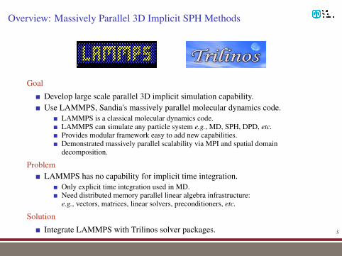
Overview: Massively Parallel 3D Implicit SPH Methods

Goal

Develop large scale parallel 3D implicit simulation capability.Use LAMMPS, Sandia's massively parallel molecular dynamics code.

LAMMPS is a classical molecular dynamics code.LAMMPS can simulate any particle system e.g., MD, SPH, DPD, etc.Provides modular framework easy to add new capabilities.Demonstrated massively parallel scalability via MPI and spatial domaindecomposition.

ProblemLAMMPS has no capability for implicit time integration.

Only explicit time integration used in MD.Need distributed memory parallel linear algebra infrastructure:e.g., vectors, matrices, linear solvers, preconditioners, etc.

Solution

Integrate LAMMPS with Trilinos solver packages. 5

Trilinos

Open source C++ software framework for solving large scale multi-physicsscientific and engineering problems: https://trilinos.org .

Developed and maintained by Sandia National Labs.Trilinos is made of packages:

The current Trilinos library consists of more than 50 packages.Each package is an independent piece of software but inter-operates with otherpackages.Use a set of packages as needed, like LEGO blocks.

By Alan Chia (Lego Color Bricks) CC BY-SA 2.0 via Wikimedia Commons.

6

LAMMPS/Trilinos Integration

Communication- Sync ghost regions- Reneighbor particles

Pair: compute- SPH operators: - Poisson Boltzmann - Navier Stokes - Transport equation

Fix: time advance- Move particles

Atom: Initialization- Distribute particles over processors

Dist. Objects- Epetra Package

LAMMPS Workflow

Preconditioners- ML (AMG)- Ifpack (Incomplete LU)

Linear Solvers- Belos (Krylov solver)- AztecOO (Krylov solver)

Nonlinear Solvers- NOX (Newton solver)

Trilinos Solver

Linear systems

State vectors

Let each code handle what it was designed to do well

LAMMPS handles particle data, parallel data distribution, ghosting.

Trilinos handles distributed memory linear solvers, preconditioners, etc.

Developed implicit solver and time integration framework can be applied to anyparticle based models in LAMMPS. 7

Smoothed Particle Hydrodynamics

8

Meshfree Particle methods

Mesh: a list of points with theirconnectivities.

Motivation of meshfree methods

Generating a suitable mesh is a challenging task.

Easier to handle large deformation, movingboundary and fluid structure interaction problemsthan grid-based approaches.

By advecting points in Lagrangian form, thenon-linear advection term in Navier Stokesequations can be removed.

9

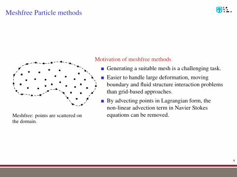
Meshfree Particle methods

Meshfree: points are scattered onthe domain.

Motivation of meshfree methods

Generating a suitable mesh is a challenging task.

Easier to handle large deformation, movingboundary and fluid structure interaction problemsthan grid-based approaches.

By advecting points in Lagrangian form, thenon-linear advection term in Navier Stokesequations can be removed.

9

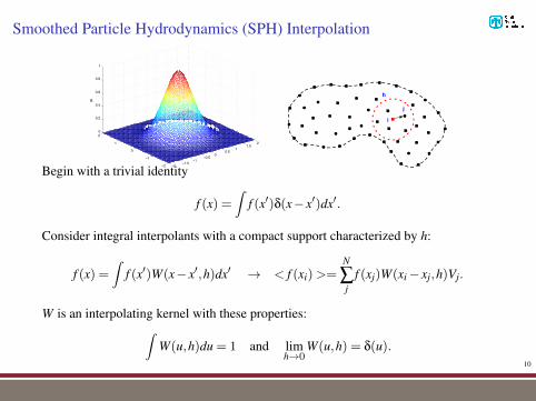
Smoothed Particle Hydrodynamics (SPH) Interpolation

−2−1.5

−1−0.5

00.5

11.5

2

−2

−1

0

1

20

0.2

0.4

0.6

0.8

1

W

i

j

h

Begin with a trivial identity

f (x) =∫

f (x′)δ(x− x′)dx′.

Consider integral interpolants with a compact support characterized by h:

f (x) =∫

f (x′)W(x− x′,h)dx′ → < f (xi)>=N

∑j

f (xj)W(xi − xj,h)Vj.

W is an interpolating kernel with these properties:∫W(u,h)du = 1 and lim

h→0W(u,h) = δ(u).

10

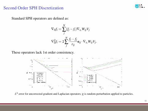
Second Order SPH Discretization

Standard SPH operators are defined as:

∇0fi =N

∑j(fj − fi)∇xi WijVj

∇20fi = 2

N

∑j

fi − fjrij

eij ·∇xi WijVj.

These operators lack 1st order consistency.

L2 error for uncorrected gradient and Laplacian operators; χ is random perturbation applied to particles.

11

Second Order SPH Discretization

The “corrected” SPH scheme uses correction tensors to obtain 1st order consistency:

∇1fi =N

∑j(fj − fi)Gi∇xi WijVj,

∇21fi = 2

N

∑j

(Li : eij ⊗∇xi Wij

)( fi − fjrij

eij ·∇1fi

)Vj,

where the correction tensors G and L are derived from a Taylor expansion2.

L2 error for “corrected” gradient and Laplacian operators; χ is random perturbation applied to particles.

[1] N.Trask et al.“A scalable consistent second-order SPH solver for unsteady viscous flows”, CMAME 2015. 12

Implementation of Navier Stokes Equations

13

Projection Scheme

Consider a incompressible flow governed by the Navier-Stokes (NS) equations:

dudt

=−1

ρ∇p+ν∇

2u+g,

∇ ·u = 0,

where g is a body force. Splitting the equations into prediction/correction steps, we

get:

Helmholtz

u∗−un

∆t=−1

ρ∇pn +ν∇

2

(u∗+un

2

)+g x ∈Ω,

u∗ = u∂Ω x ∈ ∂Ω,

Corrector

un+1−u∗

∆t=−1

ρ∇(pn+1−pn) x ∈Ω,

∇ ·un+1 = 0 x ∈Ω,

un+1 ·n = u∂Ω ·n x ∈ ∂Ω.

14

Projection Scheme

Splitting the equations into prediction/correction steps, we get:

Helmholtz

u∗−un

∆t=−1

ρ∇pn +ν∇

2

(u∗+un

2

)+g x ∈Ω,

u∗ = u∂Ω x ∈ ∂Ω,

Corrector

un+1−u∗

∆t=−1

ρ∇(pn+1−pn) x ∈Ω,

∇ ·un+1 = 0 x ∈Ω,

un+1 ·n = u∂Ω ·n x ∈ ∂Ω.

By taking the divergence of the second set of equations, we obtain the Poissonproblem for the pressure difference:

Poisson

−1

ρ∇2(pn+1−pn)=−∇ ·u∗

∆tx ∈Ω,

∇(pn+1−pn) ·n = 0 x ∈ ∂Ω.

Resulting systems of equations are solved by a preconditioned (algebraic multigrid)GMRES solver. 14

Numerical Examples3D Complex geometry: Pore-scale Flow in Bead Pack.

15

Benchmark: 3D Pore-scale Flow in Bead Pack3

The pore geometry is constructed from voxel data provided by MRI measurements.

Parameter Symbol ValueBead diagmeter d (mm) 0.5# of Beads - 6864Column diameter D (mm) 8.8Column length L (mm) 12.8Porocsity ε 0.4267Volumetric flow rate Q (kg/s) 2.771e-5Fluid density ρ (kg/m3) 997.561Fluid dynamic viscosity µ (pa− s) 8.887e-4

Flow

Steady-state solution of the flow in a bead pack.

[2] Yang. et. al., Intercomparison of 3D Pore-scale Flow and Solute Transport Simulation Methods, Advances in Water

Resources, in review. 16

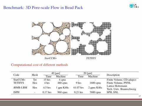
Benchmark: 3D Pore-scale Flow in Bead Pack

StarCCM+ TETHYS

Computational cost of different methods

Code Mesh40 [µm]

Time Machine20 [µm]

Time Machine Description

StarCCM+ Tet 15 hrs 4 cpus - - Finite Volume, CD-adapcoTETHYS Hex 4 hrs 480 cpus 9 hrs 1600 cpus Finite Volume, PNNL

iRMB-LBM Hex 4.5 hrs 1 gpu K40c 61.07 hrs 2 gpus K40c Lattice BoltzmannTech. Univ. Braunschweig

ISPH - 0.17 hrs 960 cpus 0.21 hrs 7680 cpus SPH, SNL17

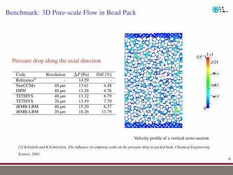
Benchmark: 3D Pore-scale Flow in Bead Pack

Pressure drop along the axial direction

Code Resolution ∆P [Pa] Diff [%]Reference4 - 14.29 -StarCCM+ 40 µm 13.61 4.48ISPH 40 µm 13.26 4.76TETHYS 40 µm 13.32 6.79TETHYS 20 µm 13.19 7.70iRMB-LBM 40 µm 15.20 6.37iRMB-LBM 20 µm 16.26 13.79

Velocity profile of a vertical cross-section.

[3] B.Eisfeld and K.Schnitzlein, The influence of confining walls on the pressure drop in packed beds, Chemical Engineering

Science, 2001.18

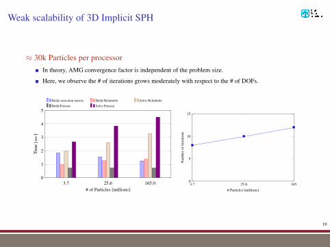
Weak scalability of 3D Implicit SPH

≈ 30k Particles per processorIn theory, AMG convergence factor is independent of the problem size.

Here, we observe the # of iterations grows moderately with respect to the # of DOFs.

3.7 25.6 165.00

1

2

3

4

5

# of Particles [millions]

Tim

e[s

ec]

Build correction tensors Build Helmholtz Solve Helmholtz

Build Poisson Solve Poisson

3.7 25.6 1650

5

10

15

# Particles [millions]

Num

bero

fite

ratio

ns

19

ConclusionDemonstrated scalable parallel Implicit SPH method.

With local correction operators, our ISPH method delivers efficient and accuratesolutions that are comparable to other numerical methods.

Implicit time integration allows to use a large time step.

Trilinos interface can be applied to problems arising from any particle-basedmodels in LAMMPS.

20

State of the Code

Discretizations:implemented second order SPH;implemented MLS with arbitrary order of approximation and ALE scheme.

Highly scalable parallel code:demonstrated the weak scalability up to 134 million particles with 32k cores;applied the implicit SPH method to solve a real problem which demands highlyintensive computation.

Muti-physics capabilities:provide capability to solve electro-kinetic flows coupled with the PoissonBoltzmann equation.

Boundary conditions:Morris mirroring technique with Holmes modification for Dirichlet BCs;continuous boundary force method proposed by Pan et al. for Robin BCs;partial slip boundary (Robin) condition with no-penetration (Dirichlet) on normaldirections;

21

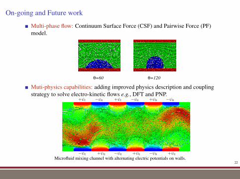
On-going and Future work

Multi-phase flow: Continuum Surface Force (CSF) and Pairwise Force (PF)model.

θ=60 θ=120

Muti-physics capabilities: adding improved physics description and couplingstrategy to solve electro-kinetic flows e.g., DFT and PNP.

+ 0 0 + 0 0 + 0 0

+ 0 0 + 0 0 + 0 0

Microfluid mixing channel with alternating electric potentials on walls.22

Thank you

This code is a researh code and we look for more collaborations for interestingapplication problems.

Acknowledgement

This work is supported by the U.S. Department of Energy Office of Science, Office ofAdvanced Scientific Computing Research, Applied Mathematics program as part ofthe Colloboratory on Mathematics for Mesoscopic Modeling of Materials (CM4),under Award Number DE-SC0009247.

This research used resources of the National Energy Research Scientific ComputingCenter, which is supported by the Office of Science of the U.S. Department of Energyunder Contract No. DE-AC02-05CH11231.

23