See discussions, stats, and author profiles for this publication at: https://www.researchgate.net/publication/23602939

Development of Turbulence Models for Shear Flows by a Double Expansion

technique.

Article  in  Physics of Fluids A Fluid Dynamics · August 1992

DOI: 10.1063/1.858424 · Source: NTRS

CITATIONS

2,201READS

2,601

5 authors, including:

Some of the authors of this publication are also working on these related projects:

Temporal Large-Eddy Simulation (TLES) View project

Siva Thangam

Stevens Institute of Technology

28 PUBLICATIONS   2,836 CITATIONS   

SEE PROFILE

T. B. Gatski

207 PUBLICATIONS   8,545 CITATIONS   

SEE PROFILE

All content following this page was uploaded by Siva Thangam on 21 May 2014.

The user has requested enhancement of the downloaded file.

AD-A240 395

F. -F Lr C T f

NASA Contractor Report 187611 S E.,

ICASE Report No. 91-65 "

ICASEDEVELOPMENT OF TURBULENCE MODELS FOR SHEARFLOWS BY A DOUBLE EXPANSION TECHNIQUE

V. YakhotS. ThangamT. B. GatskiS. A. OrszagC. G. Speziale

Contract No. NAS1-18605July 1991

Institute for Computer Applications in Science and EngineeringNASA Langley Research Center

Hampton, Virginia 23665-5225

Operated by the Universities Space Research Association

NIA 91-10664Nitional Apronit itw'n andSoqce Administration

LAngley Research Centerlanmp on, Vircpn;a 23665 5225

DEVELOPMENT OF TURBULENCE MODELS FORSHEAR FLOWS BY A DOUBLE EXPANSION TECHNIQUE

V. Yakhot*, S. Thangarntt, T. B. Gatski§,S. A. Orszag* and C. G. Speziale t

*Applied & Computational Mathematics, Princeton University, Princeton, NJ 08544tICASE, NASA Langley Research Center, Hampton, VA 23665

NASA Liigley Research Center, Hampton, VA 23665

ABSTRACT

Turbulence models are developed by supplementing the renormalization group (RNG)

approach of Yakhot & Orszag with scale expansions for the Reynolds stress and production

of dissipation terms. Th, additional expansion parameter,, (---K/ i) is the ratio of the

turbulent to mean strain time scale. While 'low-order expansions appear to provide an

adequate description for the Reynolds stress, no finite truncation of the expansion for the

production of dissipation term in powers of ;r suffices - terms of all orders must be retained.

Based on these ideas, a new two-equation model and Reynolds stress transport model are

developed for turbulent shear flows. The models are tested for homogeneous shear flow

and flow over a backward facing step. Comparisons between the model predictions and

experimental data are excellent. Aceos2:,a Y-r

•~~~~ r aIIone "' Iji-'ty CcdO8

Permanent Address: Stevens Institute of Technology, Hoboken, N.J 07030.

tThis research was supported by the National Aeronautics and Space A";;-t:2n under NASAContrt - ,S 15rn7. ,% jiie tne authors were in residence at the Institute for Computer Applicationsin Science and Engineering (t_,ASE), NASA Langley Research Center, Hampton, VA 23665.i)

I. Introduction

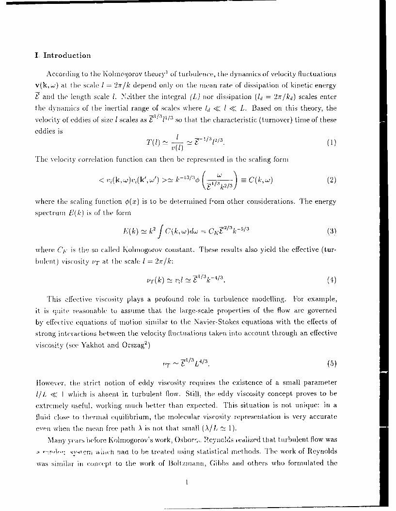
According to the Kolnogorov theory1 of turbulence, the dynamics of velocity fluctuations

v(k, .) at the scale I = 2r/k depend only oi the mean rate of dissipation of kinetic energy

E and the length scale 1. Neither the integral (L) nor dissipation (1d = 27r/kd) scales enter

the dynainics of the inertial range of scales where l,j < / < L. Based on this theory, the

velocity of eddies of size I scales as -1l/ 3 113/ so that the characteristic (turnover) time of these

eddies isT(I) j_ l z- /t3l2/ 3 (1

V(I)

The velocity correlation function can then be represented in the scaling form

< vi(k,w)vi(k',w) >- k-131 ( 1 2 C(kw) (2)

where the scaling function O(x) is to be determined f-om other considerations. The energy

spectrum E(k) is of the form

E(k) - k2JC(kw)dw = C 1 J 21 3 k- (3)

where Cj,- is the so called Kolhnogorov constant. These results also yield the effective (tur-

blulnt) viscosity VT at the scale 1 = 2r/k:

ur(, _ " , t - 4/E13113 . (4)

This effective viscosity plays a profound role in turbulence modelling. For example,

it is quite reasonable to assume that the large-scale properties of the flow are governed

by effective equations of motion similar to the Navier-Stokes equations with the effects of

strong interactions between the velocity fluctuations taken into account through an effective

viscosity (see Yakhot and Orszag2 )

'T _ -113 L 4/3. (5)

However, the strict notion of eddy viscosity requires the existence of a small parameter

I/L < 1 which is absent, in turbulent flow. Still, the eddy viscosity concept proves to be

extremely useful, working nuch better than expected. This situation is riot unique: in a

fluid close to thernral equilibriumn, the molecular viscosity representation is very accurate

even when the niean free path A is riot that snall (A/L - 1).

Many years before Kolmogorov's work, Ost)or.,, 1, {e)ynclds itidized that turbulent flow was

,!, ,crn- i, th nan to be treated using statistical methods. The work of Reynolds

was si nilar ilI concept to the work of Boltzrnarnn, Gibbs and others who formulated the

kinetic theory of gases. It was not an accident that by the early 20th century the ideas of

kinetic theory were adapted to describe turbulence with turbulent eddies as the moleculesor building blocks of this "gas." By analogy with kinetic theory the turbulent viscosity istaken to be:

VT 2- tirmsL. (6)

Combining (6) with (5) and using u _ Ums/L (so that, in the absence of turbulence pro-duction, the turbulence is damped in one large-eddy turnover time L/ums), we obtain the

K - £ model:-2

VT- = c4 (7)

where K - u-i and C, is a constant. The relation (7) is more convenient than (6) since itexpresses the turbulent viscosity through the directly measurable quantities K and F.

To implement (7) we need equations of motion for K, E and the velocity field v:

av0---+ V. _Vv = _Vp + 0VOv2 (8)OKEVV, +VV

OS + v Vi - T2 - 2vo(ViV,)(VVjp) + V 2 (10)

Otwhere p is the pressure and

T1 = 2vo(Vji)(Vj~v)(V li)

T2= 2v.(vvoV) 2 . (11)

Equations (8)-(11) must be solved subject to initial and boundary conditions as well as theincompressibility constraint V -v = 0. In order to derive equations for the mean values of Kand E, equations (8)-(11) must also be averaged over an ensemble of the fluctuating part of

the velocity field v. In the absence of a systematic averaging procedure, turbulence modellers

have used intuitive reasoning combined with experimental data, tensorial and dimensional

invariance, as well as scaling arguments based on the Kolmogorov theory 3-6 .In the siiiplk ca-, of decaying turbulence with no mean velocity field, the equation of

motion for the mean kinetic energy is usually w:iftn as:

0 K - a aK)-V + ,-V (12)

where v = vO + VT is the total viscosity and aK is a proportionality constant. The derivationof the equation for E is more difficult since it is easily shown that both T and T2 in (11) are

O(Rf.!/ 2 ) where Re., 2 /vo- = O(um.,L/vo) is the turbulence Reynolds number. However,

2

the following bold assumption (cf. Tennekes and Lumley') is fruitful: it, is assumed that the

singular contributions to T,, and T2 caacel each other in the limit as Ret -4 0o and the

remaining 0(1) part can be written as

-2

T+2 2 = (13)

where C>2 0(l). Thus, in decaying turbulence.

9 - 2 + 1 Iv E- (14)at = e2-y 4+ xK Oxi

where as = 0(1). The assumption (13) was not rigorously justified but it has led to simple

equations useful for practical calculations. In the case of homogeneous isotropic turbulence

the diffusion terms in (12) and (14) disappear yielding

Ki O t-- (1.5)

where -y = i/(C2 - 1). The fact that the coefficient C2 determines the power law of

turbulence decay demonstrates the significant role of dimensionless constants in the theory

of turbulence. Indeed, even a small error in C02 is amplified in the limit as t -4 oo. The first

term on the right side of (14) has a simple interpretation in terms of a relaxation time:

K T

whereK

is the only turbulence time-scale that one can construct from the parameters of the problem.

In flows with non-zero values of the mean strain Sij = 1(08u + au 1), the velocity field in

(8)-(11) can be decomposed into mean (U) and fluctuating (u) components. In this case the

equations of motion are typically taken to be of the form:

-+ U -VV = j --,sj - E + '9 , -a (16)OE - -- 2 0 L'xx

+ U. V = -Ce r S.- S C2 -+ (le+[ )Tt K K 4x x

Wl_: rz3 = f7 t- is the Reynolds stress tensor and the coefficients CI and C2 are constants

that are usually (1 _itClll flui- becimar' pcr,- CLs. lhe i- production term in (16)

comes from the contributions to the E - equation (10) of the type:

2ui alj S

3

which are modeled as

C eiiSij/T

in the relaxation time approximation.

There are also dyaamical constraints that a consistent turbulence model must obey. First

of all, it is obvious that

K >0, E>0. (17)

It can be shown that the conditions of realizability (17) are satisfied for homogeneous tur-

bulent flows if:dK>0, -->0

dt dt-

whenK,£ E O* .

Secondly, the turbulence model must be invariant under the Galilean transformation:

x* = X - U~t (18)

where U0 is any constant velocity. In this sense, the turbulence model must behave like

the original Navier-Stokes equations which are Galilean invariant. Any model violating

invariance under (18) is physically incorrect.

Using the simplest closure for the deviatoric part of rij:

F-2

Tij =2UTSij =-2C--Sij (19)

(where C',, 0.085 is a constant) (16) is transformed into a familiar form. It can be shown

that (16) with (19) satisfies the realizability conditions K > 0 and E > 0 provided that

C, 2 > 1 and C, > 0. These and other interesting properties of equations (16) and (19) have

been recently reviewed by Speziale s.

Let us introduce the dimensionless variables

7 = -; I -_oE ~Ko

where S = (2Sij Sij)112 and K0 is the initial turbulent kinetic energy. In homogeneous shear

flow where V2 -= 72 = 0, equations (16) and (19) have the simple form:

dK*drt - IM(CL7 - 7'

dt*

d= -C,(C, - 1)72 + (CE2 - 1) (20)

4

where t" = St. Equation (20) has a single fixed point given by

70 C 2-I -1/2 (21), = 1) (e - 1)

which is obtained by setting dil/dt = 0. This fixed point yields asymptotic solutions for Y

and of tQe fo;r M

where the growth rate A is given by'

[ , C(G 2 - Cei)2 2A [(COe- 1)(C 2 - 1) (22)

Physical and numerical experiments on homogeneous shear flow - for not too large values of

the dimensionless shear rate q - indicate that indeed, qj -- ro and K, $ cx eA ,* for t* > 1.

This means that the solutions of any turbulence model must be attracted to this fixed pointwhen r is not too large. The fact that the simp!e K - S model is capable of describing such

a non-trivial behavior is remarkable.

Another important consequence of equations (16) and (19) is the Reynolds number inde-

pendence of the von Karman constant in turbulent channel flow. It is easy to show that the

normalized dimensionless velocity profile U+ is given in the region of constant energy K +

by:+ In y+ + B (23)

where ez is the von Karman constant. The dimensionless variables y+ and U+ will be discussed

in more detail in Section IV. It follows from the model (16) and (19) that the von Karman

constant is independent of Re. This is the result of the cancellation of the singular terms

assumed in the derivation of (13). If, on the other hand T, + T2 = O(Ret/2 ) and the

assumption (13) is incorrect, then the von Karman constant K and the constant B in (23)

will depend on Ret. This would have a significant impact on engineering calculations since

(23) enters in the expression for the friction coefficient. Surprisingly, even today, there is

no compelling experimental evidence for the constancy of B and K, although the prevailing

opinion is that B and K are constants.

Now let us discuss the closure assumption (19), which can be rewritten as:

- j = -2C Km3j (24)

where qij = SijK/e is a dimensionless tensor which is equal to zero in isotropic turbulence.

When r7ij is small, the deviation from the isotropic solution is small. Unfortunately, in many

5 _ _ . . ,~ ,. • ,un ,m mu n n m nu nnunna

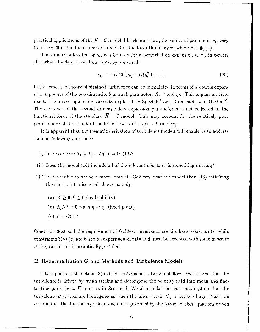
practical applications of the K - Y model, like channel flow, tie values of parameter 710 vary

from l - 20 in the buffer region to 71 - 3 in the logarithmic layer (where q] -= i11%1).

Tfie dimensionless tensor rqij can be used for a perturbation expansion of Yij in powers

of 7/ when the departures from isotropy are small:

2= Qqij + ( + ... ]. (25)

In this case, the theory of strained turbulence can be formulated in terms of a double expan-

sion in powers of the two dimensionless small parameters Re and qij. This expansion gives

rise to the anisotropic eddy viscosity explored by Speziale 9 and Rubenstein and Barton" .

The existence of the second dimensionless expansion parameter qj is not reflected in the

functional form of the standard K - S model. This may account for the relatively poo;

performance of the standard model in flows with large values of yij.

It is apparent that a systematic derivation of turbulence models will enable us to address

some of following questions:

(i) Is it true that T, + T2 = 0(1) as in (13)?

(ii) Does the model (16) include all of the relevai.t effects or is something missing?

(iii) Is it possible to derive a more complete Galilean invariant model than (16) satisfying

the constraints discussed above, namely:

(a) K > 0; S > 0 (realizability)

(b) dilldt = 0 when q --+ r (fixed point)

(c) K = 0(l)?

Condition 3(a) and the requirement of Galilean invariance are the basic constraints, while

constraints 3(b)-(c) are based on experimental data and must be accepted with some measure

of skepticism until theoretically justified.

II. Renormalization Group Methods and Turbulence Models

The equations of motion (8)-(11) describe general turbulent flow, We assume that the

turbulence is driven by mean strains and decompose the velocity field into mean and fluc-

tuating parts (v = U + u) as in Section I. We also make the basic assumption that the

turbulence statistics are homogeneous when the mean strain .ij is not too large. Next, we

assume that the fluctuating velocity field u is governed by the Navier-Stokes equations driven

6

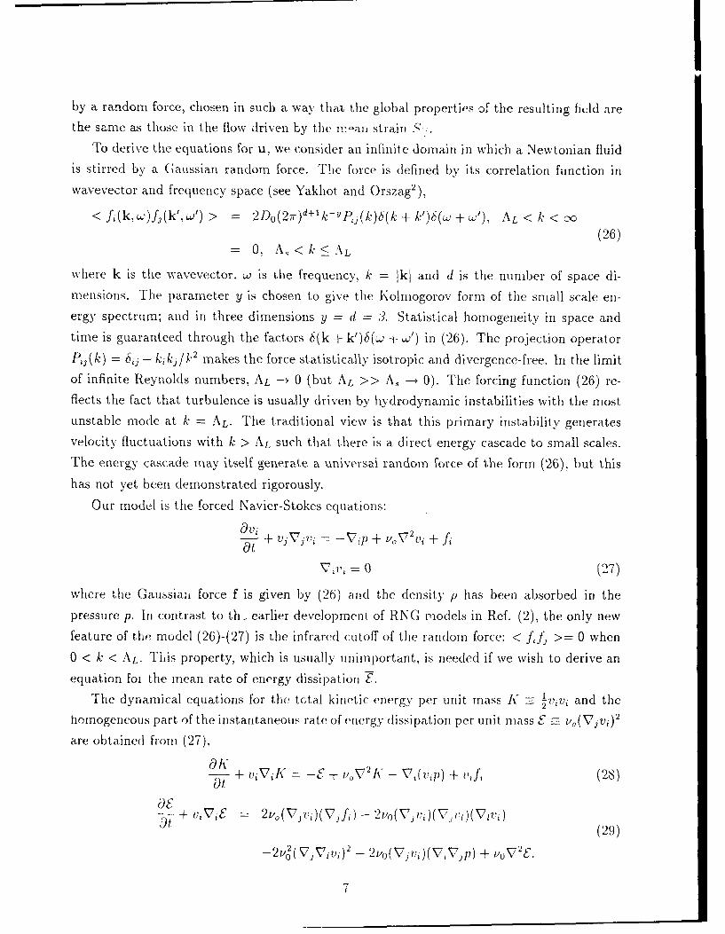
by a random force, chosen ill such a way that the global properties of the resulting field arethe same as those in the flow driven by the mnan strain ;'.-

To derive the equations for u, we consider an infinite domain in which a Newtonian fluidis stirred by a Gaussian random force. The force is defined by its correlation function in

wavevector and frequency space (see Yakhot and Orszag2 ),

< fi(k,u.)fj(k',J) > =2Do(2w)d+'k PiJ(k) (k + k' 6 (0- + A L < k <

(26)= 0, A,<k< ikL

where k is the wavevector, w is the frequency, k = Iki and d is the number of space di-

mensions. The parameter y is chosen to give the Kohlogorov form of the small scale en-ergy spectrum; and in three dimensions y = d = 3. Statistical homogeneity in space and

time is guaranteed through the factors 6(k + k')6(L, + w') in (26). The projection operator

Pij(k) = 6ij - kikj / , 2 makes the force statistically isotropic and divergence-free. In the limit

of infinite Reynolds numbers, AL -+ 0 (but AL >> A, --+ 0). The forcing function (26) re-

flects the fact that turbulence is usually driven by hydrodynamic instabilities with the most

unstable mode at k = AL. The traditional view is that this primary instability generates

velocity fluctuations with k > AL such that there is a direct energy cascade to small scales.

The energy cascade may itself generate a universal random force of the form (26), but this

has not yet been demonstrated rigorously.

Our model is the forced Navier-Stokes equations:

avi

Vivi 0 (27)

where the Gaussian force f is given by (26) and the density p has been absorbed in the

pressure p. In contrast to th. earlier development, of RNG models in Ref. (2), the only newfeature of the model (26)-(27) is the infrared cutoff of the randoln force: < fJfj >= 0 when

0 < k < AL. This property, which is usually unimportant, is needed if we wish to derive an

equation fot the mean rate of energy dissipation .

The dynamical equations for the tctal kinetic energy per unit mass K = 1civi and thehomogeneous part of the instantaneous rate of energy dissipation per unit mass S =.(VjV,)

2

are obtained from (27),

OK- + viVi[ = -,F + v0VIK - Vi(vp) + v'if, (28)

+ v, Vi 2v,( V v)( V3 ) -(29)

-2v ( 7Vz,,) 2 - 2Vo(Vj,,)(VVp) + v0VS.

7

InI thle equation for S, driven by large-scale featuores such as boundary and initial coni-

ditions, T, balances T,. to leading order. As we shiall see, for steady-state flows (27)-(29) is

sustained by the force f; T1% is balanced by both 1, anl 'lie randon i-force contribution to the

8l- roduction given by - z2v0 (Vjv;)(Vjfj)

We seek equnations for the mean values U =-< v >, K =< K > ali( S- =< E >, averaged

over an ensemble of tine jiuctitating velocity field. 1F0 find these equationls, We Shall use the

dynamic renornalization group and the 5-expaitsin. Since the renormalized equations for

K and E may niot be trivially related to the renormalized Navier-Stokes equations, the 1lANG

lprocevlure maist be app~liedl to all of the equations (27)- (29).Thie rertormalizat io!i grol p applied to ( 28)-( 29) is diescribed in tletai 1 in Yakhot an(1

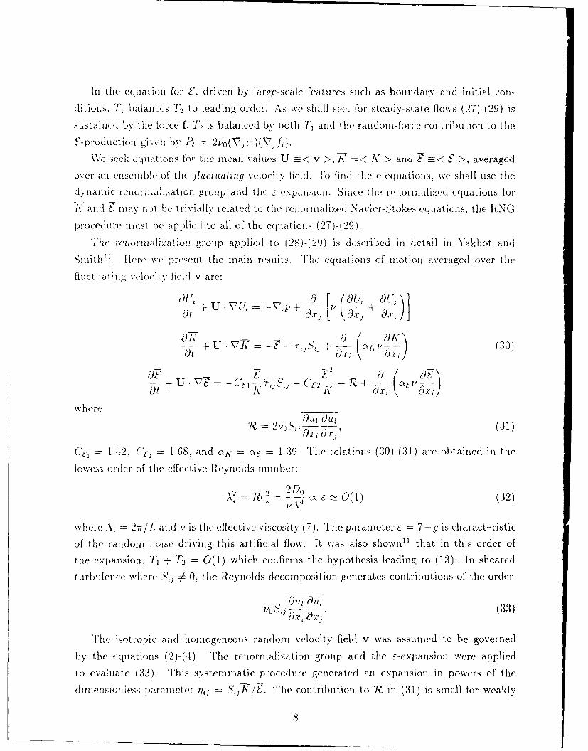
Smith"'. I lere we present the mnain results,. Thne equations of motion averaged over thle

fluctuatingo velocity field v aire:

C,: a [(&U, 5Lj + L

-+ U VK J, 0 1jS ± (ixV a)(30)

+ U - VS = -Cem= TiSi - ("-2=5 + RAl

where

CE- 1-429 C,,, 1.=68, and OK =OE 1.39. The relations (30)-(:31) are( obtained in the

lowest order of the effective Reynolds number:

where Al = 2 w/L amnd v is the effective viscosity (7). The paramreters-= 7-y is charact-ristic

of the random noise driving this artificial flow. It was also shown"' that in this order of

the expansion. T + T 2 =0(l) which confirms the hypothesis leading to (13). In sheared

turbulence where S 0, the Reynolds (decomnposition generates contributions of the order

Vo)i 011 011 (33)

T'he isotropic and homogeneous randomn velocity field v was assuniedl to be governed

by the equations (2)-(1). Thle renornialization grouip anid thle E-expansion were applied

LO evaluate (33). This systemniatic procedlure generated an expansion in powers of thle

dlinerisoni ess parameter 71hj =SijK/IF. The contribution to '1v in (31 ) is smiall for weakly

St aile(I t urbulence and large iII tle rapidI (listort loll lii it whe 1 7 -. OC. sif at teipts to

close (31) using tihe methods based on tle --ex va siori were fruitless. In Ie next sectit We

shall show how to evaluate (31 ) bly applyiNg 1i g eneral criteria outlined in Section 1.

III. Generalized K - F model

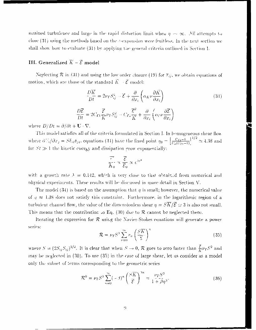
Negflecting ' in (31) and using the low order :losure (19) for f, , we obtain equations of

motion, which are those of the standard 1 - E model:

- a /

- C> )=VTS -~= + v

) t K Ox axi)where D/ Dt = a/at + U • V.

This niodel satisfies all of the criteria formulated in Section I. In ,miogeneous shear flow

whete 6 */Ox = S&,16 2.equations (34) iuxve the fixed point qo = 'I-J /2 4.38 and

for St >> 1 the kinetic energy and dissipation grow exponentially:

X C X CXA 0 so

witl: a growth rate ,\ 0.12; wh;-h is very close to thai o')tain\,d from numerical and

ohysical experiments. These results will be discussedl in more detail in Section V.

The model (3-1) is based on the assumpition tht q is smuall; however, the numerical value

of ./ ; -1.38 does not satisfy this constraint. Furthermore, in the logarithmic region of a

turbulent channel flow, the value of the dirnelsionless shear i = SI/$ - 3 is also not small.

This means that the contribution o Eq. (30) due to R? cannot be neglected there.

Iterating the expression for R using the Navier-Stokes ectuations will generate a power

series:

n

1Z=O \ /

wtere .5' = (2SSia)I1/ . It is clear that when S5 --- 0, R goes to zero faster than 1"T .C2 andmay be neglected in (30). To use (35) in the case of large shear, let us consider as a model

only thi, subset of terns corresponding to Iho geoietric series

1,=,- v- 3 , 1) 7 1+'' (36)

RI II VTI II k I II II II

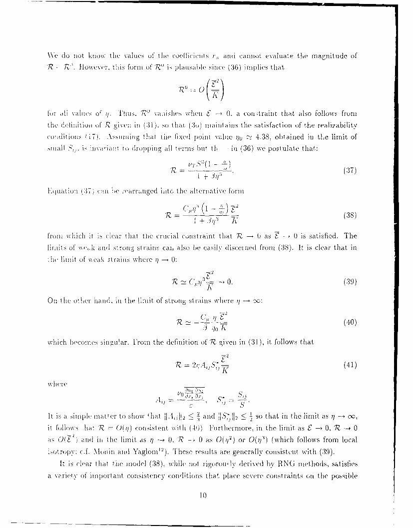
W\e (10 not know thle values of the coefficeeits 1,, ano cannot eValuiate the magnitude of

7? N. However, this form of 7 ?U iS plauISable sinice (:36) Implies that

for alIl valuies 0o 1/. -1,ii1s. R' \a aishies when C - 0 a cond raint~ that also follows from

thle deli nit ionl of R iviv 11i1 (31), so that ( 3 u) maintains the satisfaction of the realizability

co!1di tionls (17). Assnu fil lig that tiie fixed point value q() - 4.:38, obt ained 'in the limit of

sin all >,is jilva-ia ut to dIropp)ing all terms b,,t tf M i (36) we post ulate that:

i/.V )l - -1-) (7

Equat ioi (37) can h e wearrzaiged iatc, t he alterit ative [ormn

(7 Z( - w1 -i 3j~(38)

from which it is clear that the crucial constraint that R- 0 as C *0 is satisfied. The

hlii's of' wx-k andl strong strains can, also be easilv (liscel nedl from (38). It, is clear that in

hle limit of weak st rains where qj --- 0:

7Z 3 0. (39)

On the othler hand. in the L'mit, of strong strains w\here q~ -*z:

7? '~ "(40)

3 ;/o K

which becomes slinguar. From the definition of R? given in (31 ),it follows that

-2

R' 2,,AjS. (41)

I s a simple matter to show hat. fl-Aj , < fl and 1,5*11 < so that in the limit as q-4 CC

it foliows -hai 7Z? (() consiste nt w~ith (i (N) Furthermore, in the limit as S 0, 1Z-? 0-- 03(~ -, an i 1 h ii si ?- 0 ((12) or O(7/3) (which follows from local

..sotropy: cf. Mown i andI Yaglotn ). 1Th(ese results are generally consistetnt with (39).

It Is (lear that lie mnodel (38), while not ri goroucly derived by IING nmethods, satisfies

a variety of im1port a ut. consistency conditions that. place severe constraints on the posible

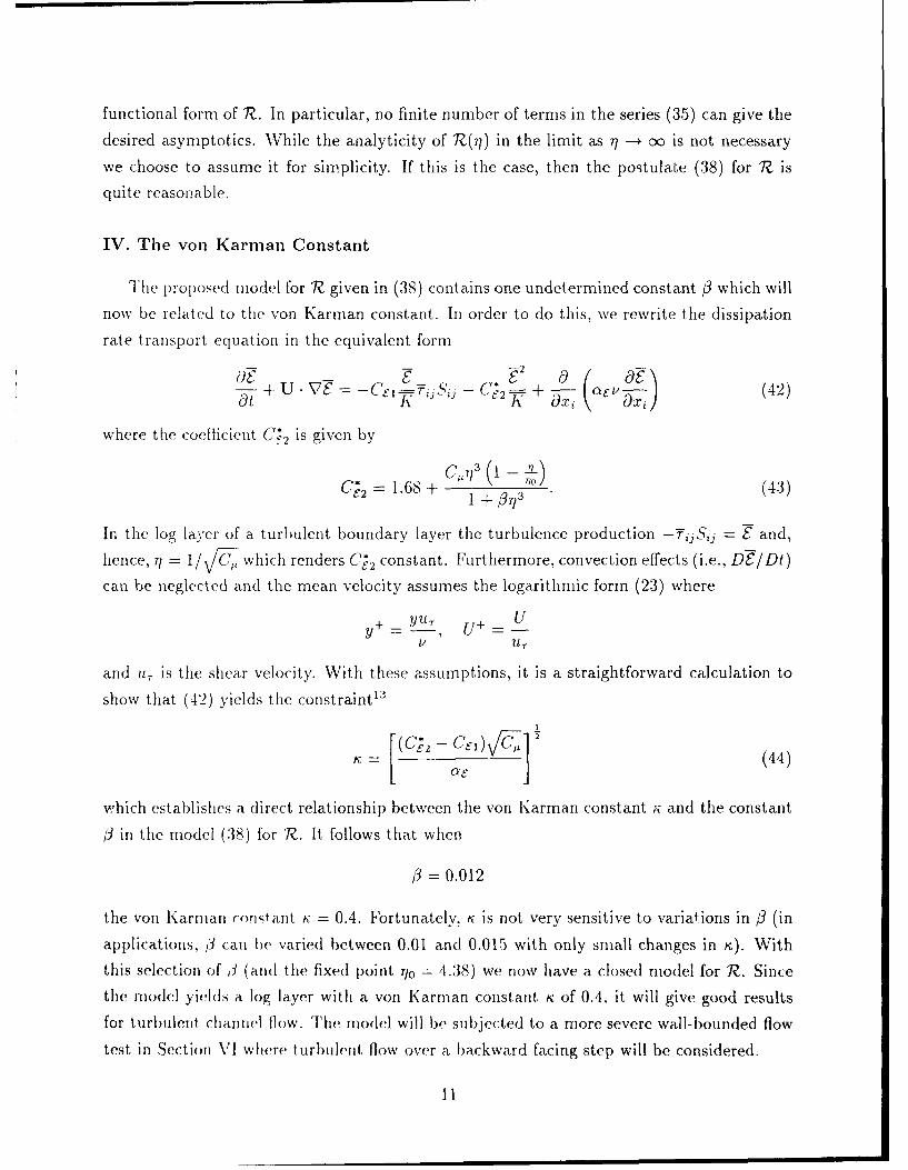
functional form of R. In particular, no finite number of terms in the series (35) can give the

desired asymptotics. While the analyticity of 7Z(i) in the limit as 77 c+0 is not necessary

we choose to assume it for simplicity. If this is the case, then the postulate (38) for 7? is

quite reasonable.

IV. The von Karman Constant

The proposed model for R given in (38) contains one undetermined constant 3 which will

now be related to the von Karman constant. In order to do this, we rewrite tile dissipation

rate transport equation in the equivalent form

2

+U -U. - 2 + ae (42)at K K Oxi x

where the coefficient C*2 is given by

C2 = 1.68 + - 770-(43)

In the log la-,er of a turbulent boundary layer the turbulence production -EijSij and,

hence, 7 1/ FC, which renders C2 constant. Furthermore, convection effects (i.e., D.F/Dt)

can be neglectedl and the mean velocity assumes the logarithmic form (23) where

y+_ yu, UY UJ+

1/ U,

and u is the shear velocity. With these assumptions, it is a straightforward calculation to

show that (42) yields the constraint 3

(Q2 - C ), 1=~ [c jl (44)

which establishes a direct relationship between the von Karman constant ;i and the constant

in the model (38) for R. It follows that when

= 0.012

the von Karinan ,ori'tant K = 0.4. Fortunately, K is not very sensitive to variations in f (in

applications, j3 can be' varied between 0.01 and 0.015 with only small changes in r,). With

this selection of I (and the fixed point 70 = 4.38) we now have a closed model for 7?. Since

the model yields a log layer with a von Karrnan constant K of 0.4. it will give good results

for turbulent channel flow. The rnodel will be subjected to a more severe wall-bounded flow

test in Section VI where turbulent flow over a backward facing step will be considered.

11

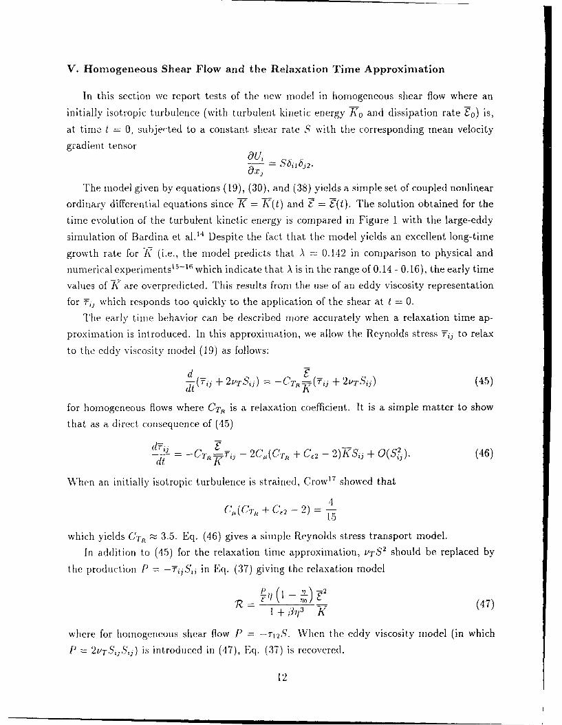
V. Homogeneous Shear Flow and the Relaxation Time Approximation

In this section we report tests of the new nodel in homogeneous shear flow where an

initially isotropic turbulence (with turbulent kinetic energy K 0 and dissipation rate E0) is,

at time t = 0, subje,'ted to a constant shear rate S with the corresponding mean velocity

gradient tensorOUi

Oxj

The model given by equations (19), (30), and (38) yields a simple set of coupled nonlinear

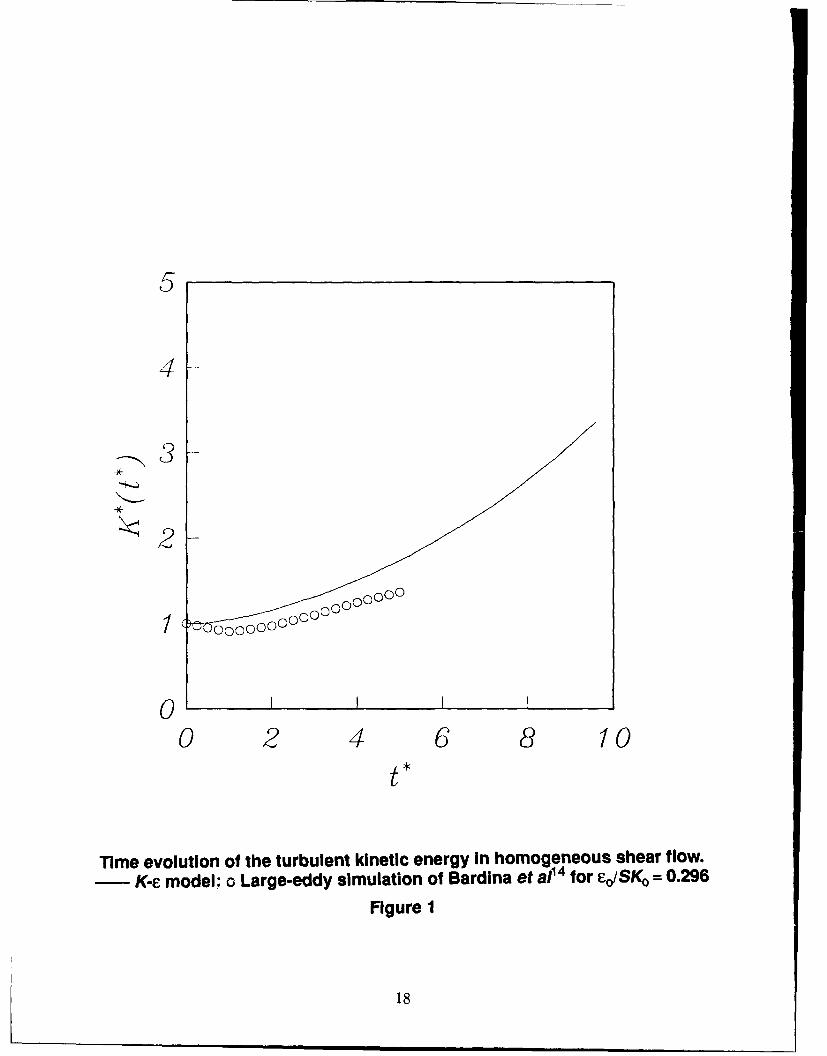
ordinary differential equations since K = (t) and S = E(t). The solution obtained for the

time evolution of the turbulent kinetic energy is compared in Figure 1 with the large-eddy

simulation of Bardina et al. 4 Despite the fact that the model yields an excellent long-time

growth rate for K (i.e., the model predicts that A = 0.142 in comparison to physical and

numerical experiments 15 -1 6 which indicate that A is in the range of 0.14 - 0.16), the early time

values of K are overpredicted. This results from the use of an eddy viscosity representation

for Tij which responds too quickly to the application of the shear at t = 0.

The early time behavior can be described more accurately when a relaxation time ap-

proximation is introduced. In this approximation, we allow the Reynolds stress Tij to relax

to the eddy viscosity model (19) as follows:

d (-(Tij + 2 PTSj) ±= -CT (Yj + 2VTSij)

for homogeneous flows where CT, is a relaxation coefficient. It is a simple matter to show

that as a direct consequence of (45)

d-fi j -9= -CTR £fj - 2C,,(CT,, + C 2 - 2)KSij + j (46)

When an initially isotropic turbulence is strained, Crow 17 showed that

4CG(CT,, + C, 2 - 2) = 4

1,5

which yields C1' ; 3.5. Eq. (46) gives a simple Reynolds stress transport model.

In addition to (45) for the relaxation timc approximation, vTS2 should be replaced by

the production P = -TijSii in Eq. (37) giving the relaxation model

1z e( - 71 (47)1 + jJ713

where for homogeneous shear flow P = -Tr2S. When the eddy viscosity model (in which

P) = 2v7-SjjSij) is introduced in (47), Eq. (37) is recovered.

12

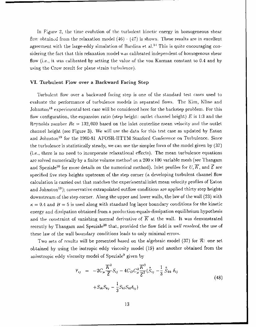
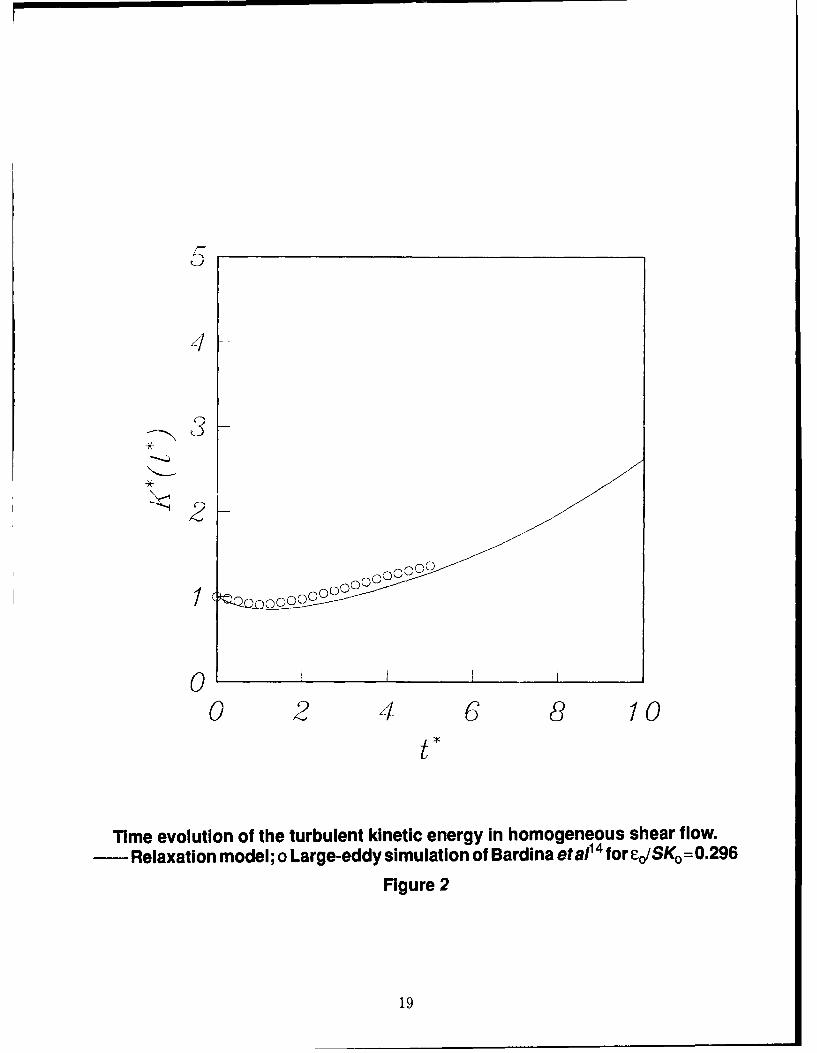
In Figure 2, the time evolution of the turbulent kinetic energy in homogeneous shear

flcxw obtaincd from the relaxation model (46) - (47) is shown. These results are in excellent

agreement with the large-eddy simulation of Bardina et al. 14 This is quite encouraging con-

sidering the fact that this relaxation model was calibrated independent of homogenous shear

flow (i.e., it was calibrated by setting the value of the von Karman constant to 0.4 and by

using the Crow result for plane strain turbulence).

VI. Turbulent Flow over a Backward Facing Step

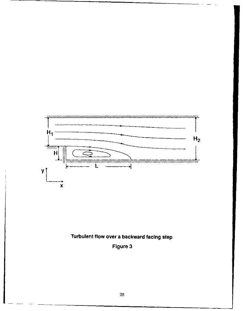
Turbulent flow over a backward facing step is one of the standard test cases used to

evaluate the performance of turbulence models in separated flows. The Kim, Kline and

Johnston1 8 experimental test case will be considered here for the backstep problem. For this

flow configuration, the expansion ratio (step height: outlet channel height) E is 1:3 and the

Reynolds number Re = 132, 000 based on the inlet centerline mean velocity and the outlet

channel height (see Figure 3). We will use the data for this test case as updated by Eaton

and Johnston19 for the 1980-81 AFOSR-HTTM Stanford Conference on Turbulence. Since

the turbulence is statistically steady, we can use the simpler form of the model given by (37)

(i.e., there is no need to incorporate relaxational effects). The mean turbulence equations

are solved numerically by a finite volume method on a 200 x 100 variable mesh (see Thangam

and Speziale2" for more details on the numerical method). Inlet profiles for U, Y, and E are

specified five step heights upstream of the step corner (a developing turbulent channel flow

calculation is carried out that matches the experimental inlet mean velocity profiles of Eaton

and Johnston1 9); conservative extrapolated outflow conditions are applied thirty step heights

downstream of the step corner. Along the upper and lower walls, the law of the wall (23) with

K= 0.4 and B = 5 is used along with standard log layer boundary conditions for the kinetic

energy and dissipation obtained from a production-equals-dissipation equilibrium hypothesis

and the constraint of vanishing normal derivative of K at the wall. It was demonstrated

recently by Thangam and Speziale2" that, provided the flow field is well resolved, the use of

these law of the wall boundary conditions leads to only minimal errors.

Two sets of results will be presented based on the algebraic model (37) for 7z: one set

obtained by using the isotropic eddy viscosity model (19) and another obtained from the

anisotropic eddy viscosity model of Speziale 9 given by

-2 -3- -20--I C K 0 1 o

-Tij =- -2C - - S j - 4CDC -U-(Sij -- Skk 5ij(48)

+SkSk 1 - 1dSklSkbi6j)

13

13 I

0

where Sij is the Oldroyd derivative of Sij with convective effects neglected; CD is a dimen-

sionless constant which assumes a value of 1.68. For thin shear layers, this model is very

similar to the anisotropic eddy viscosity model derived by Rubenstein and Bartonl ° based

on RNG methods. This type of anisotropic eddy viscosity model is obtained when terms of

order rli2 are maintained in the expansion (23) for TO.

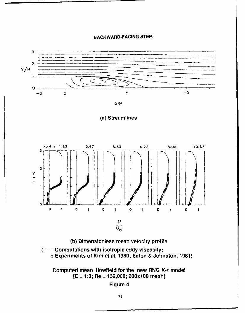
In Figures 4(a)-(b), the computed mean velocity streamlines and mean velocity profiles

obtained using the isotropic eddy viscosity model (19) are compared with the experimental

data." Reattachment is predicted at XR/H - 6.6, a result that is within 6% of the ex-

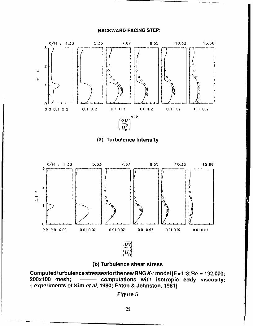
perimentally measured reattachment point XR/H - 7.0. The computed turbulence intensity

and turbulence shear stress profiles are compared with experimental data in Figures 5(a)-(b).

The agreement is comparably good.

By combining the model (37) for R with the anisotropic eddy viscosity model (48), even

better results are obtained. In Figures 6(a)-(b), the predicted mean velocity streamlines

and mean velocity profiles are shown to compare extremely favorably with the experimental

data.19 The model predicts reattachment at XR/H 7.0 which is essentially the same as

the experimental result. Furthermore, the model predicts a noticeable secondary separation

bubble below the corner of the step consistent with experimental observations for this back-

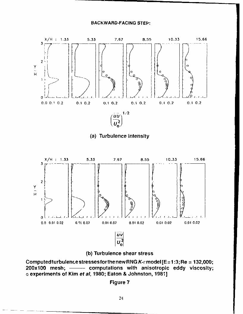
step flow. The agreement between the model predictions and the experimental data for the

turbulence intensity and turbulence shear stress profiles is also excellent as shown in Figures

7(a)-(b). The quality of these predictions is quite remarkable for a two-equation model.

VII. Concluding Remarks

The renormalization group formalism of Yakhot & Orszag for the development of turbu-

lence models has been supplemented with scale expansions for the Reynolds stress and pro-

duction of dissipation terms. Here, the extra expansion parameter is taken to be i/= SKIE

which is ratio of the turbulent to mean strain time scale. For the Reynolds stress, this

approach - which leads to the development of anisotropic eddy viscosity models as well

as Reynolds stress transport models - is analogous to that introduced by Rubenstein and

Barton. 0 However, the present method is completely new for the modelling of the production

of dissipation term 1? which is neglected in most of the commonly used turbulence models.

The interesting result for 7 is that no finite order truncation of the expansion satisfies the

necessary physical constraints; terms of all orders in the expansion must be retained. This

complication eliminates the possibility of determining the model explicitly in closed form.

However, a highly plausible form, with only one undetermined constant, is postulated here

which satisfies all of the necessary physical constraints (i.e., realizability and consistency with

14

the weak and strong strain limits). The constant is calibrated by setting the von Karman

constant K to 0.4.

The new models have been tested for homogeneous shear flow and for flow over a back-

ward facing step. Excellent results are obtained in both cases. For the case of homogeneous

shear flow, the best results are obtained from the Reynolds stress transport model (i.e., the

relaxational model discussed in Section V). On the ol er hand, excellent results are ob-

tained with eddy viscosity models for the backstep problem. In all of these calculations, no

ad hoc adjustments of the constants are made. The applications considered ill the paper are

restricted to simple shear flows since the current version of the dissipation rate transport

equation has only been modelled to account for the effects of irrotational strains. Incorpora-

tion of the effects of rotational strains, which can be important in turbulent flows involving

curvature or a system rotation, is a difficult task that has not yet been achieved. The reduc-

tion in the energy cascade that occurs in rotating isotropic turbulence and the stabilizing

or destabilizing effects of rotations on homogeneous shear flow are but two examples.21 2 2

This more difficult problem of accounting for rotational strains using a comparable scale

expansion technique will be the subject of a future study.

Acknowledgements

Two of the authors (VY and SAO) would like to acknowledge support from the Defense

Advanced Research Projects Agency under Contract N00014-86-K-0759 and from the Office

of Naval Research under Contracts N00014-82-C-0451 and N00014-90-C-0039.

15

References

1 Kolmogorov, A. N. Izv. Acad Sci. USSR, Phys. 6, 56 (1942).

2 Yakhot, V. and Orszag, S. A. J. Sci. C'ornp. 1, 3 (1986).

'Lumley, J. L. Adv. Appi. Mech. 18, 123 (1978).

'Reynolds, W. C. Lecture Notes for von Karmian Institute. AGARD Lect. 5cr. No. 86, p.

1 (NATO, New York, 1987).

'Launder, B. E. and Spaiding, D. B. Comput. Methods Appi. Mech. Eng. 3, 269 (1974).

'Launder, B. E., Reece, G. J., and Rodi, W. J. Fluid Mech. 68, 537 (1975).

'Tennekes, H1. and Lumley, J. L. A First Course in Turbulence (MIT Press, Cambridge,MA, 1972).

'Speziale, C. G. Ann. Rev. Fluid Mech. 23, 107 (1991).

'Speziale, C. G. J. Fluid Mech. 178, 459 (1987).

"Rfubenstein, ft. and Barton, J. M. Phys. Fluids A 2, 1472 (1990).

"Yakhot, V. and Smith, L. M. Phys. Fluids A, submitted for publication.

'2 Monin, A. S. and Yaglom, A. M. Statistical Fluid Mechanics: Mechanics of Turbulence,Vol. 2 (MIT Press, Cambridge, MA, 1975).

13 Patel, V. C., Rodi, W., and Scheuerer, G. AIAA J. 23, 1308 (1985).

"Bardina, J., Ferziger, J. H., and Reynolds, W. C. Stanford University Technical Report

No. TF-19 (1983).

'5 Tavoularis, S. and Corrsin, S. J. Fluid Mech. 104, 311 (1981).

"6Rogers, M. M., Moin, P., and Reynolds, W. C. Stanford University Technical Report

TF-25 (1986).

17 Crow, S. C. J. Fluid Mech. 33, 1 (1968).

"8 Kim, J., Kline, S. J., and Johnston, J. P. ASME J. Fluids Eng. 102, 302 (1980).

"9 Eaton, J. and Johnston, J. P. Stanford University Technical Report MD-39 (1980).

16

2 0Thangarn, S. aad Speziale, C. G. AIAA J., to appeal.

2 1 flardina, J., f,(rziger, J. HI., and Rogallo, R. S. J. Fluid Mfech. 154, 321 (1985).

21 Speziale, C. G. and Mac Giolla Mhuiris, N. Phys. Fluids A 1, 294 (1989).

17

5

4

*

0 I I I

0 2 4 6 8 10

t

Time evolution of the turbulent kinetic energy in homogeneous shear flow.K-E model: o Large-eddy simulation of Bardina et a114 for eoISKo = 0.296

Figure 1

18

4 --

0 I

0 2 4 6 8 10

t

Time evolution of the turbulent kinetic energy in homogeneous shear flow.Relaxation model; o Large-eddy simulation of Bardina eta 1 4 for co/SKo= 0.296

Figure 2

19

IlI

H- L -1

y

x

Turbulent flow over a backward facing step

Figure 3

20

BACKWARD-FACING STEP:

3.

Y/H

-2 0 5 10

X/H

(a) Streamlines

X/H 1.33 2.67 5.33 6.22 8.00 10.67

2 .Y

H

0 1 0 1 0 1 0 1 0 1 0

U

(b) Dimensionless mean velocity profile

-- Computations with isotropic eddy viscosity;o Experiments of Kim et al, 1980; Eaton & Johnston, 1981)

Computed mean f lowfield for the new RNG K-c model[E = 1:3; Re = 132,000; 200x100 mesh]

Figure 4

21

BACKWARD-FACING STEP:

X/H 1.33 5.33 7.67 8.55 10.33 15.663

2

y 0

H 0000

0 0o o' o- i

0 I 1 I_ L- L J - -. fI _L.. _ 1 _ -

0.0 0.1 0.2 0.1 0.2 0.1 0.2 0.1 0.2 0.1 0.2 0.1 0.2

1/2

(a) Turbulence Intensity

X/H 1.33 5.33 7.67 8.55 10.33 15.663

2Y

H 0 0

0 I !-_IL -- 1 AL - •L __ =L-1-1- - l- - _1_

0.0 0.01 0.0i 0.01 0.02 0.01 0.02 0.01 0.02 0.01 0.02 0.01 0.02

(b) Turbulence shear stress

Computedturbulence stresses forthe new RNG K-e model [E = 1:3; Re = 132,000;200x100 mesh; computations with isotropic eddy viscosity;o experiments of Kim et al, 1980; Eaton & Johnston, 1981]

Figure 5

22

BACKWARD-FACING STEP:

2

Y/H

-2 0 5 1

X/H

(a) Streamlines

3X/H-: 1.33 2.67 5.33 6.22 8.00 10.67

2Y

H

0 0,0

o 0 1 0 1 0

UUO

(b) Dimensionless mean velocity profile(Computations with anisotropic eddy viscosity;o Experiments A1 Kim et al, 1980; Eaton & Johnston, 1981)

Computed meat, tlowfield for the new RNG K-E model[E =1:3; Re = 132,000; 200x100 mesh]

Figure 6

23

BACKWARD-FACING STEP:

X/H 1.33 5.33 7.67 8.55 10.33 15.66

2Y 1 0

0 0 0H

0

o 1- , Io

0.0 0.1 0.2 0.1 0.2 0.1 0.2 0.1 0.2 0.1 0.2 0.1 0.2

1/2

@Z2J

(a) Turbulence intensity

X/H 1.33 5.33 7.67 8.55 10.33 15.663

2 I

YQ

H 0

1-0

0'00

0 _o I J I iI 13 1

0.0 0.01 0.02 0.11 0.02 0.01 0.02 0.01 0.02 0.01 0.02 0.01 0.02

(b) Turbulence shear stress

Computedturbulence stressesforthe new RNG K-c model [E = 1:3; Re = 132,000;200x100 mesh; computations with anisotropic eddy viscosity;o experiments of Kim et al, 1980; Eaton & Johnston, 1981]

Figure 7

24

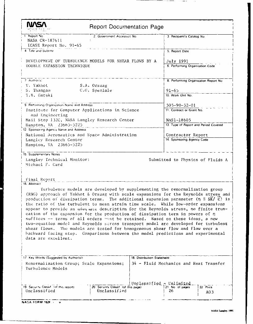
Report Documentation Page1 Report No i 2. Government Accession No. 3, Recipient's Catalog No.

NASA CR-187611ICASE Report No. 91-65

4 Tre and Sub te 5. Report Date

DEVELOPMENT OF TURBULENCE MODELS FOR SHEAR FLOWS BY A July 1991DOUBLE EXPANSION TECHNIQUE 6. Performing Organization Code

7 A u I ho r Is) .. . .8. Performing Organization Report No.

V. Yakhot S.A. Orszag

S. Thangam C.G. Speziale 91-65T.B. Gatski 10. Work Unit No.

9 Perorming Organization Name and Address 505-90-52-01

Institute for Computer Applications in Science 11. Contract or Grant No.and Engineering

Mail Stop 132C, NASA Langley Research Center NASl-18605Hampton, VA 23665-5225 13 Type of Report and Period Covered

12 Sponsoring Agency Name and Address

National Aeronautics and Space Administration Contractor ReportLangley Research Center 14. Sponsoring Agency Code

Hampton, VA 23665-5225

15 Supplementary Notes

Langley Technical Monitor: Submitted to Physics of Fluids AMichael F. Card

Final Report"6. Abstract

Turbulence models are developed by supplementing the renormalization group

(RNG) approach of Yakhot & Orszag with scale expansions for the Reynolds stress andproduction of dissipation terms. The additional expansion parameter (q E SK/ j) isthe ratio of the turbulent to mean strain time scale. While low-order expansionsappear to provide an adtq idL description for the Reynolds stress, no finite trun-cation of the expansion for the production of dissipation term in powers of risuffices -- terms of all orders r!Tst be retained. Based on these ideas, a new

two-equation model and Reynolds sLress transport model are developed for turbulentshear flows. The models are tested for homogeneous shear flow and flow over abackward facing step. Comparisons between the model predictions and experimentaldata are excellent.

r17-Key W-ds (Suggested by Authorisll 18. Distribution Statement

Renormalization Group; Scale Expansions; 34 - Fluid Mechanics and Heat Transfer

Turbulence Models

Unclassified - Unlimited"19 Security Classif (of this reporti Tb-ecurtyClassif 1of this page) 121 No of pages 22 PriceUnclassified Unclassified 26 A03

NASA FORM 162F

NASA-Lange, 1991

View publication statsView publication stats