notes 8. turbulence in thin film flows · notes 8. turbulence in thin film flows notes 8 detail the...

NOTES 8. TURBULENCE IN THIN FILM FLOWS. Dr. Luis San Andrés © 2009

1

Notes 8. Turbulence in Thin Film Flows Notes 8 detail the characteristics of turbulent flows and provide insight into the flow instabilities that precede transition from a laminar to a turbulent flow condition. Turbulence is eminently a fluid inertia driven effect, i.e. when inertia forces are much larger than viscous forces A flow instability can be of centrifugal type that induces Taylor vortices when an inner cylinder rotates, or due to wave propagation in parallel flows. In fluid film bearings, the transition from laminar to turbulent flow at a Reynolds number of ~2,000 is referential only. The Notes also provide insight into the closure problem of turbulence (how to evaluate the six components of the apparent Reynolds stresses) and explain the concept of eddy viscosity. Equations for the transport of turbulent flow kinetic energy and dissipation (κ-ε model) to determine the eddy viscosity are given. However, in thin film lubrication to this date, much simpler models are in use. Hirs’ turbulent bulk-flow model, as derived from an insightful observation that measurements in pressure and shear driven flows show similar wall shear stresses, is detailed. Hirs’ model focuses on relating the wall shear stress differences to the bulk-flow velocity components. Hence, details of turbulence transport across the film are entirely avoided. A generalized Reynolds equation, valid for either laminar or turbulent flows, is the end result of the analysis. The Notes also derive turbulent flow equations that are identical to those under laminar flow conditions, expect for the introduction of shear factors due to flow turbulence. Nomenclature C Radial clearance [m]

f m

MU hf n ρμ

⎛ ⎞= ⎜ ⎟

⎝ ⎠= n Rem. Friction factor in turbulent flow

h Film thickness m, ,n Parameters in friction factor formula p Pressure [N/m2] = ( )p p′+

,p p′ Time averaged and fluctuations of pressure [N/m2] r Surface roughness [m]R ½ D. Journal radius [m]

Re R cρ

μΩ . (Shear flow) Reynolds number

S i,j=1,2,3 1,2,31 ;2

jii

j i

uux x =

⎧ ⎫∂∂⎪ ⎪+⎨ ⎬∂ ∂⎪ ⎪⎩ ⎭. Fluid strain rate tensor [N/m2]

t Time [s]

T1 , T2 Small (fast) and large (slow) time scales for averaging of turbulent flow velocities [s]


2

Ta 2ReCR

⎛ ⎞⎜ ⎟⎝ ⎠

. Taylor number

( ) 1, 2, 3i iu = Components of velocity field [m/s] = ( )i iu u′+

( ) 1, 2, 3,i i iu u =′ Time averaged and fluctuations of velocity field [m/s]

u, v, w Components of velocity in x, y, z directions [m/s] U ΩR. Journal surface velocity [m/s] UM Mean velocity of bulk-flow [m/s]

Vx, Vz

0 0

1 1;

h h

udy wdyh h∫ ∫ . Bulk flow velocities [m/s]

ε Dissipation function in turbulent flow [m2/s2]

κ ' ' ' ' ' '1 1 2 2 3 3

12

u u u u u u⎡ ⎤+ +⎣ ⎦ . Kinetic energy of turbulent fluctuations (per unit

mass) [m2/s2] , ,

,x y

J B

κ κ

κ κ ( )1

2x z J Bκ κ κ κ= = + ; ;J J J B B Bf R f Rκ κ= = . Bulk flow turbulence

shear parameters. =12 for laminar flows ρ Fluid density [kg/m3] μ Absolute viscosity [N.s/m2]

tν 2ˆ ulV l

s∂

=∂

Turbulence eddy viscosity [m2/s]. l characteristic length,

V̂ characteristic mean flow velocity.

( ), 1,2,3ij i j

τ=

Wall shear stress tensor [N/m2]

( ) , 1,2,3tij i jτ = ( )i ju uρ ′ ′− . Reynolds (apparent) stress tensor [N/m2]

xyτΔ 0 2h

xy x x JUV

hμτ κ κ⎛ ⎞= − −⎜ ⎟⎝ ⎠

. Wall shear stress difference x-direction

(N/m2)

zyτΔ ( )0

hzy z zV

hμτ κ= − . Wall shear stress difference z-direction (N/m2)

σ i,j=1,2,3 Stress tensor [N/m2] Ω Journal rotational speed (rad/s) Subscript B Bearing J Journal c Critical value Superscript - Time average ‘ Fluctuating value


3

The characteristics of flow turbulence Turbulent fluid flow motion is an irregular flow condition in which the various flow quantities (velocity, pressure, temperature, etc.) show a random variation in time and space, but in such a way that statistically distinct averages can be discerned (Hinze, 1959). The forms of the largest eddies (low-frequency fluctuations) are usually determined by the flow boundaries, while the form of the smallest eddies (highest frequency fluctuations) are determined by the viscous forces (Roddi, 1980).

The characteristics of fluid turbulence observed in nature are, according to Abbott and Basco (1989) and Tennekes and Lumley (1981): Irregularity: Flow too complicated to be fully described with detail and economically. Deterministic approaches are impossible (to date). Three Dimensionality: Turbulence is always rotational and flow fluctuations have three-dimensional components even if the mean flow is one or two-dimensional. Turbulence flows always exhibit high levels of fluctuating vorticity. Diffusivity: Rapid mixing and increased rates of momentum, heat, mass transfer, etc. Dissipation: The kinetic energy of turbulence is dissipated to heat under the influence of viscosity since viscous shear stresses perform mechanical deformation work that increases the internal energy of the fluid. The energy source to produce turbulence must come from the mean flow by interaction of shear stresses and velocity gradients.

Once turbulence initiates, it cannot sustain itself, but depends on its flow environment to provide its energy. Large Reynolds Numbers: Turbulence is a fluid flow feature that occurs at high Reynolds numbers; it is not a property of the particular fluid itself. Turbulence often originates as a form of instability of the laminar flow if the Reynolds number becomes too large. These instabilities are related to the interaction of viscous and inertia forces. Turbulence is generally anisotropic, i.e. its intensity varies in each spatial direction. Some simple flows have a limited range of eddy scales and may be idealized as isotropic, or independent of direction. Usually only the very smallest turbulence scales can be properly idealized as homogeneous, i.e. independent of the spatial location.

Figure 1. Volcanic eruption in Ecuador (10/1999). The largest turbulent jet/plume flow ever seen


4

Turbulence is a continuum phenomenon, governed by the equations of fluid mechanics. Even the smallest scales occurring in a turbulent flow are order of magnitudes larger than any molecular length scale. Instabilities in fluid flows: Flow transition from a laminar condition to a turbulent condition is usually preceded by flow instability. In isothermal flows, instability arises in two basic forms: 1. Centrifugal Instability: occurs in flows with curved streamlines when the destabilizing

(centrifugal) force exceeds in magnitude the stabilizing (viscous) force. This instability is characterized by a steady secondary laminar flow often referred as Taylor-Gortler vortices.

2. Parallel Flow Instability: characterized by propagating waves. Here the fluid inertia force

is destabilizing and the viscous force is stabilizing, thus the Reynolds number is a parameter of importance. Examples are found in shear flows such as in jets and boundary-wall flows such as in pipes.

In the literature of thin film bearings (Szeri, 1980), the accepted critical value of the Reynolds number (Rec) for a parallel flow instability leading directly to flow turbulence is

Re 2,000cRCρμΩ

= ≥ (1)

where (ρ,μ) are the lubricant material density and viscosity, (R, c) are the bearing radius and clearance, and (Ω) is the journal rotational speed in rad/s. The Couette flow Reynolds number (Re) denotes the ratio between fluid inertia forces ρ (ΩR)2 and viscous forces μ (ΩR)/C in a shear flow induced by motion of a bounding surface. This criterion does not account for either side (axial) flow effects due to an imposed pressure gradient or the surface condition and macroscopic structure of the journal and bearing surfaces. The critical Reynolds number magnitude noted is referential only, strictly valid for hydrodynamic bearings operating at a near centered journal condition Even to this date, a handful of researchers claim that transition to turbulent flow in thin film journal bearings is delayed to Reynolds numbers (Rec) two orders of magnitude larger than 2,000. This uncommon assertion dismisses the large body of experimental evidence that confirms the critical value given above. Centrifugal flow instability has been studied with great detail in the flow between rotating cylinders. Experiments and analysis show that the flow is stable to centrifugal disturbances if the outer cylinder rotates and the inner cylinder is stationary. On the other hand, if the inner cylinder rotates and the outer cylinder is at rest, centrifugal instabilities can lead to flow instability depending on the value of a characteristic parameter known as the Taylor Number (Ta).


5

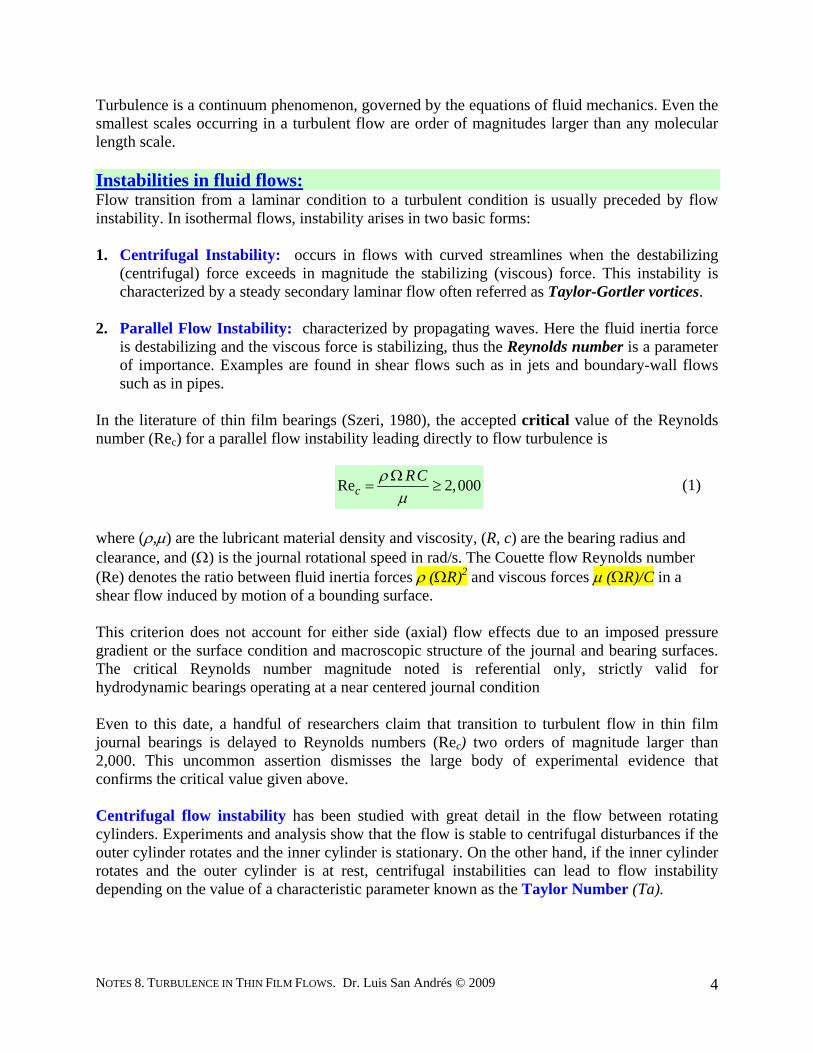
As the rotational speed (Ω) of the inner cylinder increases, the flow becomes unstable, and characterized by the appearance of toroidal vortical cells equally spaced along the spinning axis of the cylinder. These Taylor vortices greatly affect the torque required to spin the inner cylinder. The critical Taylor number (Tac) is

2Re 1,707.8a ccCTR

⎛ ⎞= =⎜ ⎟⎝ ⎠

(2)

for concentric cylinders (no eccentricity) with (C/R) <<1. In a typical thin film journal bearing, (C/R)=1/1,000, and thus the critical Reynolds number needed for the appearance of Taylor vortices is

1/2

1/2Re 41.3 1,000 1,304c cRTaC

⎛ ⎞= = × =⎜ ⎟⎝ ⎠

(3)

As the Taylor number increases above its critical value, the Taylor vortices become unstable to non-axisymmetric disturbances, i.e. the vortex cells become distorted. Szeri (1980) provides a lucid discussion on the process leading from Taylor vortex flow to the ultimate appearance of flow turbulence as the speed of the inner cylinder increases further. Note that as the ratio(R/c) increases, the transition towards turbulent flow could occur due to parallel flow instability without the appearance of Taylor vortices!

Some relevant operating conditions provide a stabilizing influence to the flow between rotating cylinders and delay the appearance of Taylor vortex flow. These conditions, predicted by complex analysis (DiPrima and Stuart, 1972) and confirmed by experiments, are:

- Axial flow due to an external pressure gradient.

Figure 2. Taylor vortices in flow between concentric rotating cylinders


6

- Operating journal eccentricity. For example at ε = e/C = 0.8 and C/R=0.010, the critical Taylor number (Tac) is about 3 times the value of 1,708 valid for concentric cylinders (ε=0).

- Circumferential pressure flow in the direction of the Couette flow, i.e., for ∂P/∂θ < 0.

Incidentally, the aspect ratio in the axial direction (L/C) appears not to have any effect on the appearance of Taylor vortices. In the design of thin film journal bearings operating at small eccentricities (ε ~ 0) it is accepted that

A parallel flow transition occurs when Re ~ 2,000. If the value of Ta½ = 41.3 is reached before the Reynolds number attains this value, then the transition is to vortex flow. However, if the flow Reynolds number, Re, exceeds 2,000 while Ta½ is still less than 41.3 then the transition is directly to turbulent flow (Seri, 1980).

Note that this criterion is valid for concentric cylinders (e=0). Appropriate criteria for journal eccentric operation is too cumbersome and given only for ideal cases. Equations of Turbulent Fluid Flow Motion Flow turbulence is a random process very difficult to model and to predict. It only “makes sense” to describe turbulence global or average behavior. This averaging may be in the time domain or space domain, both, or some other kind of meaningful ensemble procedure. For time procedures, the characteristic time for averaging must be much smaller than that typical time describing the temporal fluctuations of the mean flow. For space averaging, the physical size of the averaging volume must be much smaller than the size of the largest eddies confined within the boundaries of the mean flow. Thus, it is clear that the equations derived (and solution methods) cannot resolve below the smallest time (and space) characteristic scales. The classical theory of turbulence modeling represents the flow variables, i.e. fluid velocities (ui)i=1,2,3 and pressure (p), as the superposition of an averaged quantity (mean variable) and a fluctuating component, i.e. 3,2,1;; =′+=′+= iiii uuuppp (4) where for time averaging,

210

;)(1)( TTTduT

TuT

ii ≤≤= ∫ ττ (5)

T1 is the time scale of the “largest” eddies in the flow, and T2 is the time scale of the “slow” temporal variations of the flow that are not directly induced by turbulence.


7

Abbott and Basco (1989) provide an interesting description establishing the fallacy of Eqn. (5) in the context of the concept of a continuum. Determining a-priori the appropriate time scales T1 and T2, which depend on the flow itself can be rather cumbersome. The use of the (time) averaging process leads to a set of properties for the mean flow and fluctuation variables. These are expressed as:

; , constant

. . ; ; 0; 0

; . . 0

f g f g a f a f a

f g f g f f f f f

f f f g f gx x

+ = + = =

′= = = − =

∂ ∂ ′ ′= = =∂ ∂

(6)

The equations of flow continuity and momentum transport for an incompressible fluid are

1,2,3

, 1,2,3

0;

;

ii

i

iji ij i j

j i

ux

u uut x x

σρ ρ

=

=

∂=

∂∂∂ ∂

+ =∂ ∂ ∂

(7)

where {ui}i=1,2,3 are the fluid velocity components in the {xi}i=1,2,3 (x1=x, x2=y, x3=z) directions, σ is the stress tensor, and ρ is the fluid density. In a Newtonian fluid, the stress tensor σ is related to the fluid material viscosity (μ), the hydrodynamic pressure (p), and the rate of strain (S) by,

3,2,1,;2 =+−= jiijijij Sp μδσ (8)

1,2,31 ;2

jiij i

j i

uuSx x =

⎧ ⎫∂∂⎪ ⎪= +⎨ ⎬∂ ∂⎪ ⎪⎩ ⎭ (9)

where δij is the Kronecker-Delta function, i.e., δij=1 if i=j; 0 otherwise. Substitution of the mean and fluctuating flow field variables into Eqns. (7), and using the function properties in Eqn. (6), renders the equations of motion for the (time averaged) mean flow quantities and fluctuation fields,

'

1,2,30; 0i ii

i i

u ux x =

∂ ∂= =

∂ ∂ (10)


8

{ } , 1, 2, 32i ij ij ij i j i j

j j

u uu p S u ut x x

ρ ρ δ μ ρ =

∂ ∂ ∂ ′ ′+ = − + −∂ ∂ ∂

(11)

Osborne Reynolds derived these equations as early as in 1895. The term in parenthesis on the right hand side of Eqn. (11) represents the total mean stress tensor for the turbulent flow. The contribution of the turbulent flow motion to the mean stress tensor is usually known as the Reynolds stress tensor, 3,2,1,; =′′−= jijit uu

ijρτ (12)

This tensor has six independent components that determine the influence of the flow fluctuations into the mean flow. That is, Eqn. (12) introduces the effect of the flow fluctuations into the mean flow field. Note that the analysis thus far renders four mean flow equations, but at each spatial point in the flow field we have ten unknown variables, i.e. 1 pressure, 3 fluid velocities, and 6 components of the Reynolds stress tensor. The difference between the number of unknowns and the number of available equations makes a direct solution of any turbulent flow problem impossible. The resulting phenomenological problem of finding additional equations or conditions to make up the difference is known as the CLOSURE PROBLEM of flow turbulence.

The fundamental problem of turbulence flow modeling is to relate the six Reynolds stress components (τt) to the mean flow quantities in some physically plausible manner. This topic is, however, out of the scope of the lectures in Modern Lubrication. The interested reader may consult the fundamental references of Hinze (1959), Tennekes and Lumley (1981), Rodi(1980), Frisch (1995), and Holmes et al. (1996). Incidentally, Abbott and Basco (1989) review the initial developments in space-averaged methods leading to the formulation of the large eddy simulation (LES) models and the treatment of the Lorenz (turbulent flow) stresses. At the beginning of the 21th century, powerful computers number crunch flow turbulence without resorting to time or space or both types of averages. In addition, novel tool of mathematical analysis such as power spectral decomposition and proper orthogonal decompositions enable to predict turbulent flows in various scales (time and space wise).

Most homogenous turbulence models in the archival literature relate the Reynolds stresses to the gradient of the mean velocity vector (Rodi, 1980), i.e.

, 1,2,32 ;3ij

jit i j t ij i j

j i

uuu ux x

τ ρ ρν ρ κ δ =

⎧ ⎫∂∂⎪ ⎪′ ′= − ≈ + −⎨ ⎬∂ ∂⎪ ⎪⎩ ⎭ (13)

' ' ' ' ' ' ' '1 1 2 2 3 3

1 12 2i iu u u u u u u uκ ⎡ ⎤ ⎡ ⎤= = + +⎣ ⎦ ⎣ ⎦ (14)


9

where νt is the eddy viscosity, and κ is the kinetic energy (per unit mass) of the turbulence fluctuations. Equation (13), generally known as the Boussinesq approximation (1877), provides a mathematical model to the closure problem in flow turbulence; and shows that, just as with the viscous stresses in laminar flow, the turbulent flow stresses are proportional to the gradients of the mean (time averaged) velocities. Now, instead of six unknown turbulent shear stresses there is only one unknown, the turbulent viscosity νt, which must be determined from the flow itself. Tat is, the eddy viscosity νt is not a material property and depends strongly on the turbulence intensity, varying significantly from one spatial point to another point in the flow region, and also from one flow to another flow. Thus, substitute Eqn. (13) into the total stress (σ), Eqn. (11) , for the turbulent flow to get

, 1,2,32

31 ;jt i

ij ij i jj i

uupx x

νσ ρκ δ μν =

⎧ ⎫∂∂⎪ ⎪⎛ ⎞⎧ ⎫≈− + + + + +⎨ ⎬ ⎨ ⎬⎜ ⎟ ∂ ∂⎩ ⎭ ⎝ ⎠⎪ ⎪⎩ ⎭ (15)

Note that the term ρκ, the kinetic energy of the velocity fluctuations ( )'

1,2,3i iu

=, acts as a sort of

dynamic pressure. Hence we could define a dynamic pressure as 23

p ρκ⎡ ⎤+⎣ ⎦ . Thus, the

appearance of κ in Eqn. (15) does not need its direct determination. Note also that the flow fluctuations ( )'

1,2,3i iu

== 0 at a wall or flow boundary. Hence, any pressure measurement at a wall

does not evidence any velocity induced pressure. Most importantly, it is the distribution of the eddy viscosity vt which must be ascertained. A formulation for the eddy-viscosity (νt) in simple shear flows was conceiving an analogy between the turbulent flow motion and the molecular motions that leads to Stokes viscosity law in laminar flows. Turbulent eddies are thought as lumps of fluid which, very much like material molecules, collide and exchange momentum (Rodi, 1980). The molecular (material) viscosity (ν) is proportional to the average velocity and mean free path length of the molecules. Accordingly, by analogy, the eddy viscosity (νt) is also proportional to a velocity (V~ ) characterizing the (large scale) fluctuating motion and a typical length of this motion (l).

Vlt

ˆ≈ν (16) For shear layers with only one significant turbulent stress ( )vu ′′⋅ρ , Prandtl (1945) shows that the velocity scale is properly given by

sulV∂∂

=ˆ (17)


10

where s is the normal direction to the mean flow u . Hence, the eddy viscosity can be expressed as:

sulVlt ∂

∂== 2ˆν (18)

Thus, Prandtl’s mixing-length hypothesis relates the eddy viscosity (νt) to the gradient of the mean velocity and a single unknown parameter, the mixing length (l). Kolmogorov (1942) and Prandtl (1945) defined the mixing length. The original hypothesis extended to complex flows becomes (Rodi, 1980)

2/1

2

⎥⎥⎦

⎤

⎢⎢⎣

⎡

∂∂

⎪⎭

⎪⎬⎫

⎪⎩

⎪⎨⎧

∂

∂+

∂∂

=j

i

i

j

j

it x

uxu

xu

lν (19)

Szeri (1980) describes the turbulence flow models commonly used in fluid film bearing analyses. Most of the original research, including some fundamental experimental verification, was performed in the early 1960’s, driven by the needs of the nuclear power industry. In those days, liquid sodium bearings for nuclear reactors as well as water lubricated bearings for boiler feed pumps constituted state of the art applications with operating Reynolds numbers (Re) around 10,000. Constantinescu (1962), Ng (1964), and Elrod and Ng (1967) pioneered the analyses using the mixing-length hypothesis and implementing the law of wall to derive the fundamental length scale (l). Final results for these models are given later. The mixing length model has worked surprisingly well for many simple turbulent flows like shear layers, boundary wall flows, wakes, and also in fluid film lubrication. However, as Tennekes and Lumley (1981) point out, mixing length models are incapable of describing turbulent flows containing more than one velocity and one length scale since turbulent eddies are not rigid bodies and certainly their sizes are not small (relative to the flow domain) as required by the kinetic theory of gases. Classification of turbulence flow models Several models have evolved to determine the transport of turbulent flow quantities, thus determining the components of the Reynolds stresses. Most models employ transport equations for scalar function to characterize the eddy viscosity.

Name of Model Number of turbulent flow transport equations

Turbulence Quantities Transported

Zero equation 0 None One equation,κ 1 κ → νt (kinetic energy) Two equation, κ-ε 2 κ and ε → νt

(kinetic energy and dissipation) Stress/Flux 6

ji uu ′′ ′′ Algebraic stress 2 κ and ε → τt


11

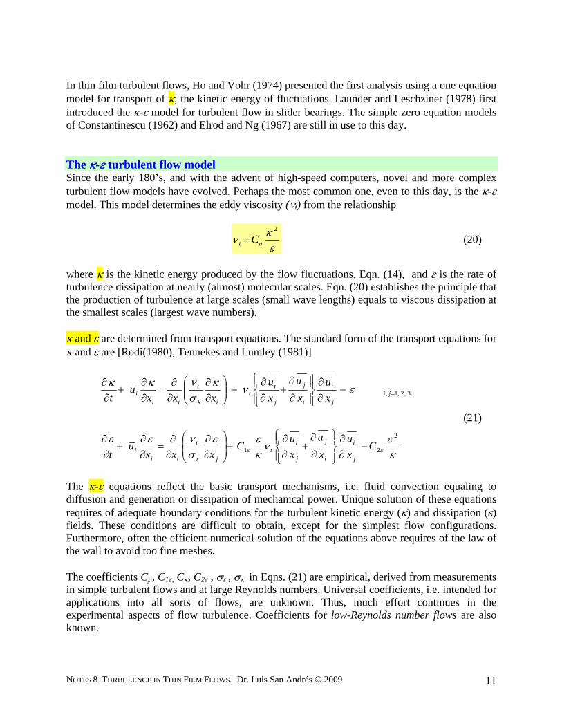
In thin film turbulent flows, Ho and Vohr (1974) presented the first analysis using a one equation model for transport of κ, the kinetic energy of fluctuations. Launder and Leschziner (1978) first introduced the κ-ε model for turbulent flow in slider bearings. The simple zero equation models of Constantinescu (1962) and Elrod and Ng (1967) are still in use to this day. The κ-ε turbulent flow model Since the early 180’s, and with the advent of high-speed computers, novel and more complex turbulent flow models have evolved. Perhaps the most common one, even to this day, is the κ-ε model. This model determines the eddy viscosity (νt) from the relationship

εκν

2

ut C= (20)

where κ is the kinetic energy produced by the flow fluctuations, Eqn. (14), and ε is the rate of turbulence dissipation at nearly (almost) molecular scales. Eqn. (20) establishes the principle that the production of turbulence at large scales (small wave lengths) equals to viscous dissipation at the smallest scales (largest wave numbers).

κ and ε are determined from transport equations. The standard form of the transport equations for κ and ε are [Rodi(1980), Tennekes and Lumley (1981)]

κεν

κεε

σνεε

ενκσνκκ

εεε

2

21

3,2,1,

Cxu

xu

xu

Cxxx

ut

xu

xu

xu

xxxu

t

j

i

i

j

j

it

j

t

iii

jij

i

i

j

j

it

ik

t

iii

−∂∂

⎪⎭

⎪⎬⎫

⎪⎩

⎪⎨⎧

∂

∂+

∂∂

+⎟⎟⎠

⎞⎜⎜⎝

⎛

∂∂

∂∂

=∂∂

+∂∂

−∂∂

⎪⎭

⎪⎬⎫

⎪⎩

⎪⎨⎧

∂

∂+

∂∂

+⎟⎟⎠

⎞⎜⎜⎝

⎛∂∂

∂∂

=∂∂

+∂∂

=

(21)

The κ-ε equations reflect the basic transport mechanisms, i.e. fluid convection equaling to diffusion and generation or dissipation of mechanical power. Unique solution of these equations requires of adequate boundary conditions for the turbulent kinetic energy (κ) and dissipation (ε) fields. These conditions are difficult to obtain, except for the simplest flow configurations. Furthermore, often the efficient numerical solution of the equations above requires of the law of the wall to avoid too fine meshes.

The coefficients Cμ, C1ε, Cκ, C2ε , σε , σκ in Eqns. (21) are empirical, derived from measurements in simple turbulent flows and at large Reynolds numbers. Universal coefficients, i.e. intended for applications into all sorts of flows, are unknown. Thus, much effort continues in the experimental aspects of flow turbulence. Coefficients for low-Reynolds number flows are also known.


12

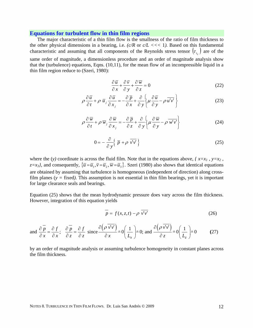
Equations for turbulent flow in thin film regions The major characteristic of a thin film flow is the smallness of the ratio of film thickness to

the other physical dimensions in a bearing, i.e. (c/R or c/L <<< 1). Based on this fundamental characteristic and assuming that all components of the Reynolds stress tensor ( )

ijtτ are of the same order of magnitude, a dimensionless procedure and an order of magnitude analysis show that the (turbulence) equations, Eqns. (10,11), for the mean flow of an incompressible liquid in a thin film region reduce to (Szeri, 1980):

0=∂∂

+∂∂

+∂∂

zw

yv

xu (22)

⎭⎬⎫

⎩⎨⎧

′′−∂∂

∂∂

+∂∂

−=∂∂

+∂∂ vu

yu

yxp

xuu

tu

jj ρμρρ (23)

⎭⎬⎫

⎩⎨⎧

′′−∂∂

∂∂

+∂∂

−=∂∂

+∂∂ vw

yw

yzp

xww

tw

jj ρμρρ (24)

{ }0 p v vy

ρ∂ ′ ′= − +∂

(25)

where the (y) coordinate is across the fluid film. Note that in the equations above, { x=x1 , y=x2 , z=x3}, and consequently, { }321 ,, uwuvuu === . Szeri (1980) also shows that identical equations are obtained by assuming that turbulence is homogeneous (independent of direction) along cross-film planes (y = fixed). This assumption is not essential in thin film bearings, yet it is important for large clearance seals and bearings. Equation (25) shows that the mean hydrodynamic pressure does vary across the film thickness. However, integration of this equation yields vvtzxfp ′′−= ρ),,( (26)

and zf

zp

xf

xp

∂∂

=∂∂

∂∂

=∂∂ ; since

( ) ( )1 10 0; and 0 0x z

v v v v

x L z L

ρ ρ′ ′ ′ ′∂ ∂⎛ ⎞ ⎛ ⎞− − − −⎜ ⎟ ⎜ ⎟∂ ∂ ⎝ ⎠⎝ ⎠

(27)

by an order of magnitude analysis or assuming turbulence homogeneity in constant planes across the film thickness.


13

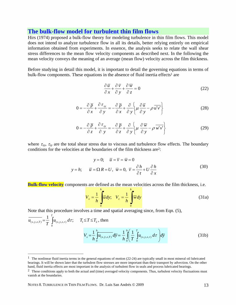
The bulk-flow model for turbulent thin film flows Hirs (1974) proposed a bulk-flow theory for modeling turbulence in thin film flows. This model does not intend to analyze turbulence flow in all its details, better relying entirely on empirical information obtained from experiments. In essence, the analysis seeks to relate the wall shear stress differences to the mean flow velocity components as described next. In the following the mean velocity conveys the meaning of an average (mean flow) velocity across the film thickness. Before studying in detail this model, it is important to detail the governing equations in terms of bulk-flow components. These equations in the absence of fluid inertia effects1 are

0=∂∂

+∂∂

+∂∂

zw

yv

xu (22)

⎭⎬⎫

⎩⎨⎧

′′−∂∂

∂∂

+∂∂

−=∂

∂+

∂∂

−= vuyu

yxp

yxp xy ρμ

τ0 (28)

⎭⎬⎫

⎩⎨⎧

′′−∂∂

∂∂

+∂∂

−=∂

∂+

∂∂

−= vwyw

yzp

yzp zy ρμ

τ0 (29)

where τxy, τzy are the total shear stress due to viscous and turbulence flow effects. The boundary conditions for the velocities at the boundaries of the film thickness are2:

0; 0

; , 0,

y u v wh hy h u R U w v Ut x

= = = =∂ ∂

= = Ω = = = +∂ ∂

(30)

Bulk-flow velocity components are defined as the mean velocities across the film thickness, i.e.

dywh

Vdyuh

V

h

z

h

x ∫∫ ==

00

1;1 (31a)

Note that this procedure involves a time and spatial averaging since, from Eqn. (5),

( , , , ) ( , , , ) 1 20

1 ;T

x y z T x y zu u d T T TT τ τ= ≤ ≤∫ , then

( , , , ) ( , , , )0 0 0

1 1 1h h T

x x y z T x y zV u dy u d dyh h T τ τ

⎛ ⎞= = ⎜ ⎟

⎝ ⎠∫ ∫ ∫ (31b)

1 The nonlinear fluid inertia terms in the general equations of motion (22-24) are typically small in most mineral oil lubricated bearings. It will be shown later that the turbulent flow stresses are more important than their transport by advection. On the other hand, fluid inertia effects are most important in the analysis of turbulent flow in seals and process lubricated bearings. 2 These conditions apply to both the actual and (time) averaged velocity components. Thus, turbulent velocity fluctuations must vanish at the boundaries.


14

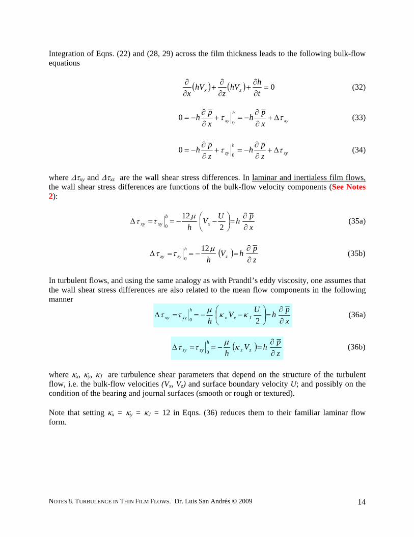
Integration of Eqns. (22) and (28, 29) across the film thickness leads to the following bulk-flow equations

( ) ( ) 0=∂∂

+∂∂

+∂∂

thhV

zhV

x zx (32)

xy

h

xy xph

xph ττ Δ+

∂∂

−=+∂∂

−=0

0 (33)

zy

h

zy zph

zph ττ Δ+

∂∂

−=+∂∂

−=0

0 (34)

where Δτxy and Δτxz are the wall shear stress differences. In laminar and inertialess film flows, the wall shear stress differences are functions of the bulk-flow velocity components (See Notes 2):

xphUV

h x

h

xyxy ∂∂

=⎟⎠⎞

⎜⎝⎛ −−==Δ

212

0

μττ (35a)

( )zphV

h z

h

zyzy ∂∂

=−==Δμττ 12

0 (35b)

In turbulent flows, and using the same analogy as with Prandtl’s eddy viscosity, one assumes that the wall shear stress differences are also related to the mean flow components in the following manner

xphUV

h Jxx

h

xyxy ∂∂

=⎟⎠⎞

⎜⎝⎛ −−==Δ

20κκμττ (36a)

( )zphV

h zz

h

zyzy ∂∂

=−==Δ κμττ0

(36b)

where κx, κy, κJ are turbulence shear parameters that depend on the structure of the turbulent flow, i.e. the bulk-flow velocities (Vx, Vz) and surface boundary velocity U; and possibly on the condition of the bearing and journal surfaces (smooth or rough or textured). Note that setting κx = κy = κJ = 12 in Eqns. (36) reduces them to their familiar laminar flow form.


15

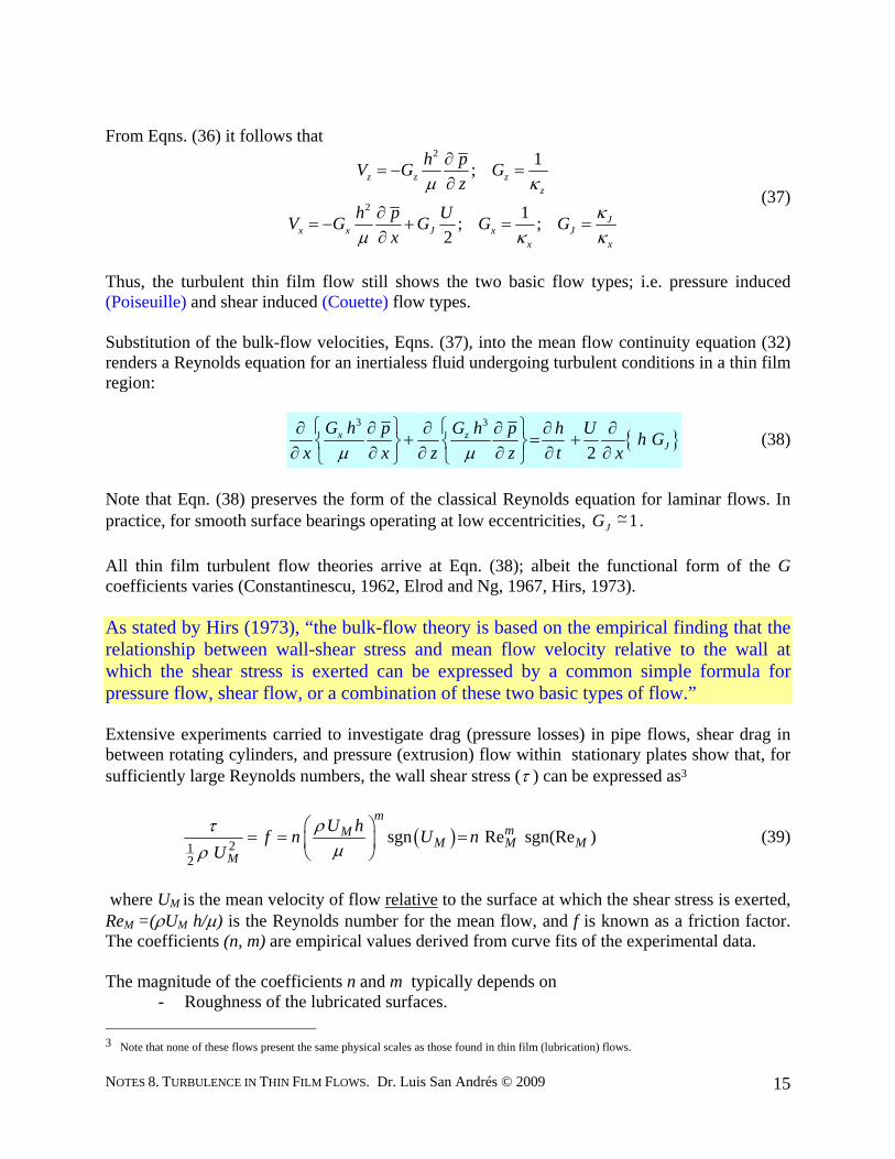
From Eqns. (36) it follows that

2

2

1;

1; ;2

z z zz

Jx x J x J

x x

h pV G Gz

h p UV G G G Gx

μ κ

κμ κ κ

∂= − =

∂

∂= − + = =

∂

(37)

Thus, the turbulent thin film flow still shows the two basic flow types; i.e. pressure induced (Poiseuille) and shear induced (Couette) flow types. Substitution of the bulk-flow velocities, Eqns. (37), into the mean flow continuity equation (32) renders a Reynolds equation for an inertialess fluid undergoing turbulent conditions in a thin film region:

{ }3 3

2x z

JG h G hp p h U h G

x x z z t xμ μ⎧ ⎫ ⎧ ⎫∂ ∂ ∂ ∂ ∂ ∂

+ = +⎨ ⎬ ⎨ ⎬∂ ∂ ∂ ∂ ∂ ∂⎩ ⎭⎩ ⎭ (38)

Note that Eqn. (38) preserves the form of the classical Reynolds equation for laminar flows. In practice, for smooth surface bearings operating at low eccentricities, 1~−JG . All thin film turbulent flow theories arrive at Eqn. (38); albeit the functional form of the G coefficients varies (Constantinescu, 1962, Elrod and Ng, 1967, Hirs, 1973). As stated by Hirs (1973), “the bulk-flow theory is based on the empirical finding that the relationship between wall-shear stress and mean flow velocity relative to the wall at which the shear stress is exerted can be expressed by a common simple formula for pressure flow, shear flow, or a combination of these two basic types of flow.” Extensive experiments carried to investigate drag (pressure losses) in pipe flows, shear drag in between rotating cylinders, and pressure (extrusion) flow within stationary plates show that, for sufficiently large Reynolds numbers, the wall shear stress (τ ) can be expressed as3

( )212

sgn Re sgn(Re )m

mMM M M

M

U hf n U nU

ρτμρ

⎛ ⎞= = =⎜ ⎟

⎝ ⎠ (39)

where UM is the mean velocity of flow relative to the surface at which the shear stress is exerted, ReM =(ρUM h/μ) is the Reynolds number for the mean flow, and f is known as a friction factor. The coefficients (n, m) are empirical values derived from curve fits of the experimental data. The magnitude of the coefficients n and m typically depends on

- Roughness of the lubricated surfaces. 3 Note that none of these flows present the same physical scales as those found in thin film (lubrication) flows.


16

- Magnitude of the flow Reynolds number. - Influence of inertia effects other than those inherent in the flow turbulence. - The type of flow, shear or pressure driven.

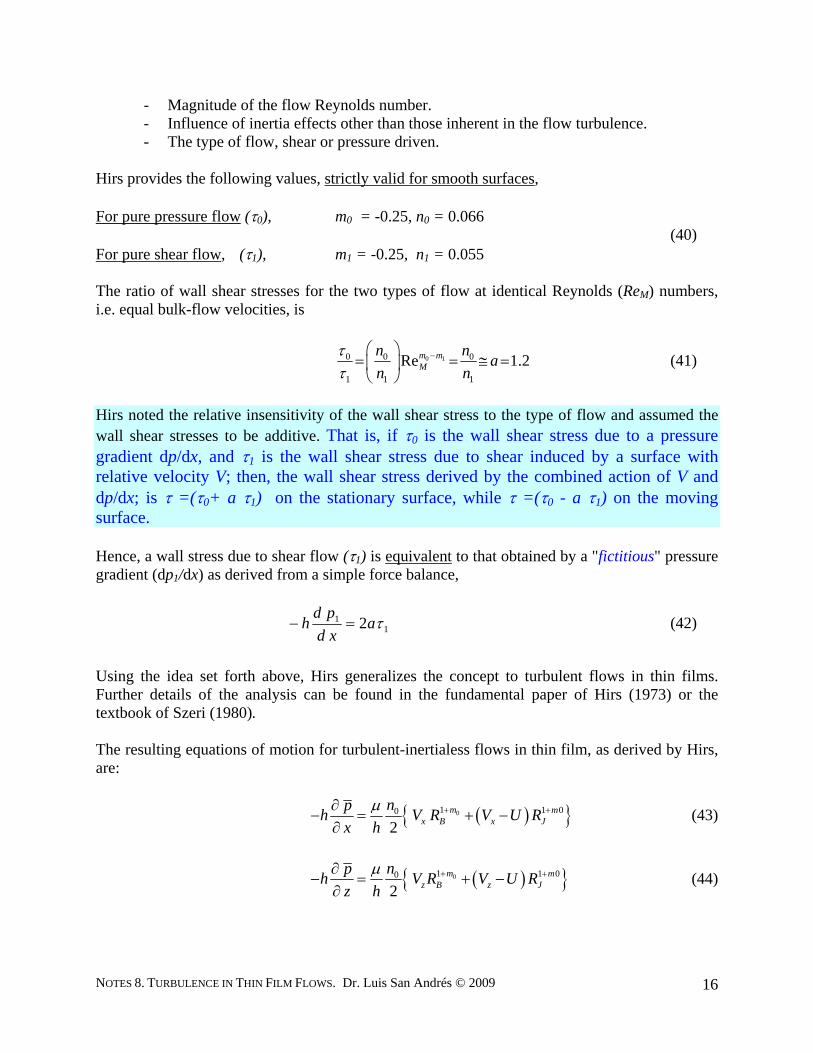
Hirs provides the following values, strictly valid for smooth surfaces, For pure pressure flow (τ0), m0 = -0.25, n0 = 0.066 (40) For pure shear flow, (τ1), m1 = -0.25, n1 = 0.055 The ratio of wall shear stresses for the two types of flow at identical Reynolds (ReM) numbers, i.e. equal bulk-flow velocities, is

0 10 0 0

1 1 1

Re 1.2m mM

n n an n

ττ

−⎛ ⎞= = ≅ =⎜ ⎟⎝ ⎠

(41)

Hirs noted the relative insensitivity of the wall shear stress to the type of flow and assumed the wall shear stresses to be additive. That is, if τ0 is the wall shear stress due to a pressure gradient dp/dx, and τ1 is the wall shear stress due to shear induced by a surface with relative velocity V; then, the wall shear stress derived by the combined action of V and dp/dx; is τ =(τ0+ a τ1) on the stationary surface, while τ =(τ0 - a τ1) on the moving surface. Hence, a wall stress due to shear flow (τ1) is equivalent to that obtained by a "fictitious" pressure gradient (dp1/dx) as derived from a simple force balance,

11 2 τa

xdpd

h =− (42)

Using the idea set forth above, Hirs generalizes the concept to turbulent flows in thin films. Further details of the analysis can be found in the fundamental paper of Hirs (1973) or the textbook of Szeri (1980). The resulting equations of motion for turbulent-inertialess flows in thin film, as derived by Hirs, are:

( ){ }01 1 00

2m m

x B x Jnph V R V U R

x hμ + +∂

− = + −∂

(43)

( ){ }01 1 00

2m m

z B z Jnph V R V U R

z hμ + +∂

− = + −∂

(44)


17

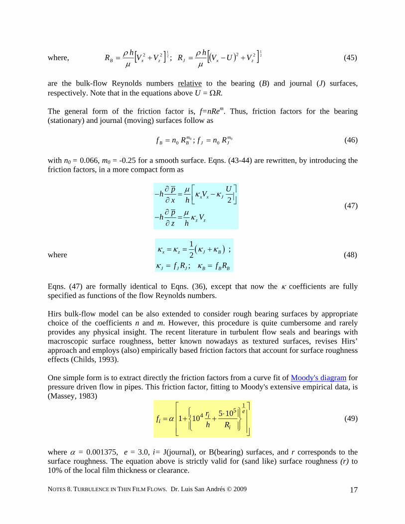
where, [ ] ( )[ ] 21

21

2222 ; zxJzxB VUVhRVVhR +−=+=μρ

μρ (45)

are the bulk-flow Reynolds numbers relative to the bearing (B) and journal (J) surfaces, respectively. Note that in the equations above U = ΩR. The general form of the friction factor is, f=nRem. Thus, friction factors for the bearing (stationary) and journal (moving) surfaces follow as

0000 ; m

JJmBB RnfRnf == (46)

with n0 = 0.066, m0 = -0.25 for a smooth surface. Eqns. (43-44) are rewritten, by introducing the friction factors, in a more compact form as

2x x J

z z

p Uh Vx hph Vz h

μ κ κ

μ κ

∂ ⎡ ⎤− = −⎢ ⎥∂ ⎣ ⎦∂

− =∂

(47)

where ( )1 ;2;

x z J B

J J J B B Bf R f R

κ κ κ κ

κ κ

= = +

= = (48)

Eqns. (47) are formally identical to Eqns. (36), except that now the κ coefficients are fully specified as functions of the flow Reynolds numbers. Hirs bulk-flow model can be also extended to consider rough bearing surfaces by appropriate choice of the coefficients n and m. However, this procedure is quite cumbersome and rarely provides any physical insight. The recent literature in turbulent flow seals and bearings with macroscopic surface roughness, better known nowadays as textured surfaces, revises Hirs’ approach and employs (also) empirically based friction factors that account for surface roughness effects (Childs, 1993).

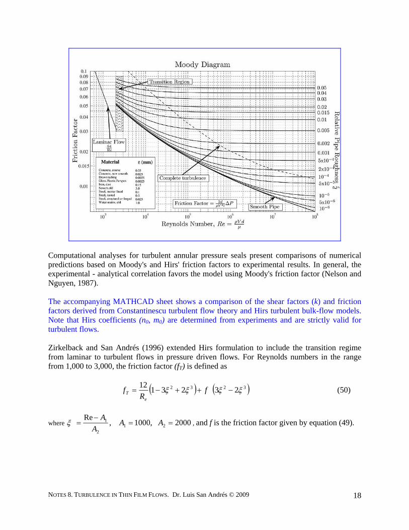
One simple form is to extract directly the friction factors from a curve fit of Moody's diagram for pressure driven flow in pipes. This friction factor, fitting to Moody's extensive empirical data, is (Massey, 1983)

15

4 5 101 10e

ii

i

rfh R

α⎡ ⎤

⎧ ⎫⋅⎪ ⎪⎢ ⎥= + +⎨ ⎬⎢ ⎥⎪ ⎪⎩ ⎭⎢ ⎥⎣ ⎦

(49)

where α = 0.001375, e = 3.0, i= J(journal), or B(bearing) surfaces, and r corresponds to the surface roughness. The equation above is strictly valid for (sand like) surface roughness (r) to 10% of the local film thickness or clearance.


18

Computational analyses for turbulent annular pressure seals present comparisons of numerical predictions based on Moody's and Hirs' friction factors to experimental results. In general, the experimental - analytical correlation favors the model using Moody's friction factor (Nelson and Nguyen, 1987).

The accompanying MATHCAD sheet shows a comparison of the shear factors (k) and friction factors derived from Constantinescu turbulent flow theory and Hirs turbulent bulk-flow models. Note that Hirs coefficients (n0, m0) are determined from experiments and are strictly valid for turbulent flows. Zirkelback and San Andrés (1996) extended Hirs formulation to include the transition regime from laminar to turbulent flows in pressure driven flows. For Reynolds numbers in the range from 1,000 to 3,000, the friction factor (fT) is defined as

( ) ( )3232 2323112 ξξξξ −++−= fR

fe

T (50)

where 2000 ,1000 ,Re

212

1 ==−

= AAA

Aξ , and f is the friction factor given by equation (49).


19

Closure The trends towards high speed bearing and seal applications and using process fluids and gases, as opposed to mineral oils, determines operating conditions well within the turbulent flow regime. Constantinescu’s model is preferred to model turbulent flow in journal and thrust bearings. Hirs’ turbulent bulk-flow including fluid inertia effects has been used extensively to predict the flow characteristics and rotordynamic coefficients of annular pressure seals and externally pressurized (hydrostatic) bearings. In general, predictions compare well with measurements for smooth surface seals and bearings.

Computational analyses based on the bulk-flow model for complex seal geometries such as labyrinth seals and honeycomb damper seals predict well the static characteristics (leakage and power dissipation) but perform poorly in the estimation of rotordynamic force coefficients, for example. It appears that the friction factors in these seal configurations are more complicated functions of the Reynolds number and surface conditions (macroscopic or “machined” roughness) than the simple formulas advanced by Hirs. Incidentally, the bulk-flow model does very well in flows without strong recirculations or very curved streamlines. Note that honeycomb and labyrinth seals present zones of local recirculation that are not accounted for in the bulk-flow model. References Abbot, M., and Basco, D., 1989, “Computational Fluid Mechanics,” Longman Scientific and Technical Pubs., London, UK. Childs, D., 1993, “Turbomachinery Rotordynamics,” John Wiley and Sons, NY. Hinze, J., 1959, “Turbulence,” McGraw-Hill Pubs., NY. Constantinescu, V.N., 1962, “Analysis of Bearings Operating in the Turbulent Flow Regime,” ASME Journal of Lubrication Technology, Vol. 82, pp. 139-151. DiPrima, R.C., and J.T. Stuart, 1972, “Non Local Effects in the Stability of Flow Between Eccentric Rotating Cylinders”, Journal of Fluid Mechanics, Vol. 54, pp. 393-415. Elrod, H.G., and C.W. Ng, 1967, “A Theory for Turbulent Films and its Applications to Bearings,” ASME Journal of Lubrication Technology, Vol. 89, pp. 346-362. Frisch, U., 1995, “Turbulence,” Cambridge University Press, U.K. Hirs, G.G., 1973, “A Bulk-Flow Theory for Turbulence in Lubricant Films,” ASME Journal of Lubrication Technology, Vol. 94, pp. 137-146.


20

Ho, M.K., and J.H. Vohr, 1974, “Application of an Energy Model of Turbulence to Calculation of Lubricant Flows,” ASME Journal of Lubrication Technology, Vol. 96, pp. 95-102. Holmes, P., J. L. Lumley, and G. Berkooz, 1996, “Turbulence, Coherent Structures, Dynamical Systems and Symmetry,” Cambridge Monographs on Mechanics, Cambridge University Press, U.K. Launder, B. and M. Leschziner, 1978, “Flow in Finite Width, Thrust Bearings Including Inertial Effects, I: Laminar Flow, II: Turbulent Flow,” ASME Journal of Lubrication Technology, Vol. 100, pp. 330-345. Massey, B.S., 1983, “Mechanics of Fluids” Van Nostrand Reinhold (UK) Co. Ltd., pp. 213. Nelson, C., and D., Nguyen, 1987, “Comparison of Hir’s equation with Moody’s Equation for Determining Rotordynamic Coefficients of Annular Pressure Seals,” ASME Journal of Tribology, Vol. 109, pp. 144-148. Ng, C. W., 1964, “Fluid Dynamic Foundation of Turbulent Lubrication Theory,” STLE Transactions, Vol. 7, pp. 311-321. Rodi,W., 1980, “Turbulence Models and Their Applications in Hydraulics,” IAHR Monograph, June. Szeri, A., 1980, “Tribology: friction, lubrication, and wear,” Mc Graw Hill Pubs. Tennekes, H., and J.L., Lumley, 1981, “A First Course in Turbulence,” The MIT Press, Cambridge, MA. Zirkelback, N., and L. San Andrés, 1996, "Bulk-Flow Model for the Transition to Turbulence Regime in Annular Seals," STLE Tribology Transactions, Vol.39, 4, pp. 835-842.


21

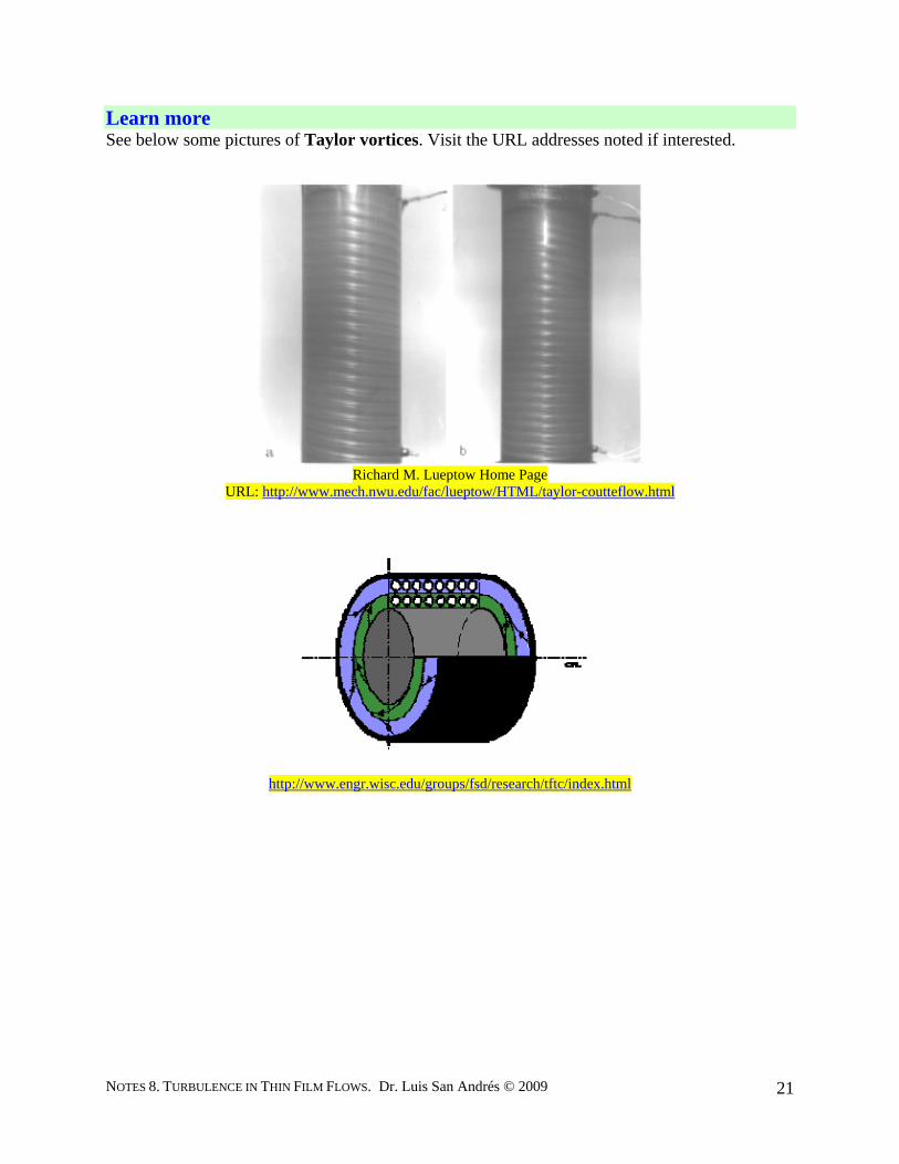
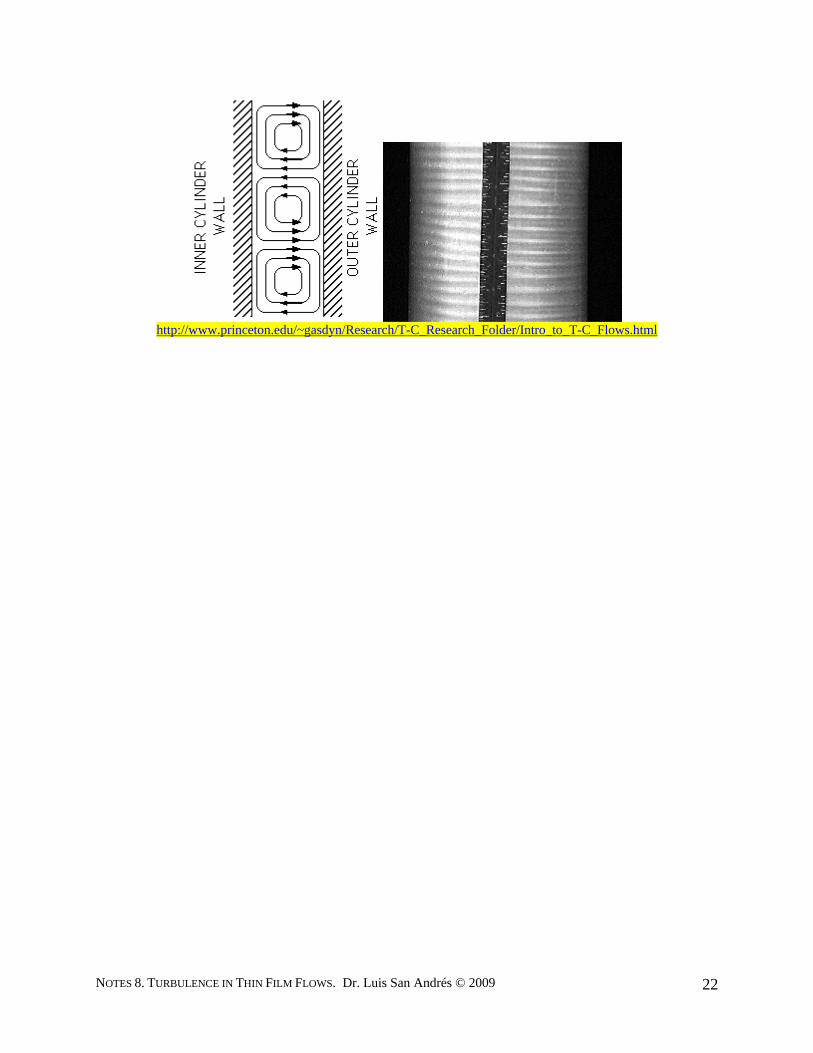
Learn more See below some pictures of Taylor vortices. Visit the URL addresses noted if interested.

Richard M. Lueptow Home Page

URL: http://www.mech.nwu.edu/fac/lueptow/HTML/taylor-coutteflow.html

http://www.engr.wisc.edu/groups/fsd/research/tftc/index.html


22

http://www.princeton.edu/~gasdyn/Research/T-C_Research_Folder/Intro_to_T-C_Flows.html

100 1 .103 1 .104 1 .10510

100

1 .103

ConstantinescuHirs

Couette flow shear factors (kz)

Couette Reynolds number

κzC Rei( )κzH Rei( )

Rei

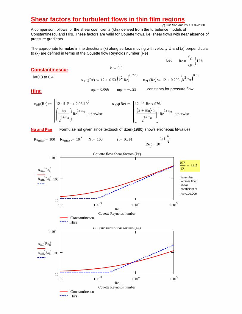
times the laminar flow shear coefficient at Re=100,000

40212

33.5=

100 1 .103 1 .104 1 .10510

100

1 .103

ConstantinescuHirs

Couette flow shear factors (kx)


κxC Rei( )κxH Rei( )

Rei

Rei 101 i

4

N⋅+

:=i 0 N..:=N 100:=Remax 105

:=Remin 100:=

Formulae not given since textbook of Szeri(1980) shows erroneous fit-valuesNg and Pan

κxH Re( ) 12 Re 976.<if

2 m0+( ) n0⋅

21 m0+

⎡⎢⎢⎣

⎤⎥⎥⎦

Re1 m0+

⋅ otherwise

:=κzH Re( ) 12 Re 2.06 103⋅<if

n0

21 m0+

⎛⎜⎜⎝

⎞⎟⎟⎠

Re1 m0+

⋅ otherwise

:=

Hirs: constants for pressure flowm0 0.25−:=n0 0.066:=

κzC Re( ) 12 0.296 k2 Re⋅( )0.65⋅+:=κxC Re( ) 12 0.53 k2 Re⋅( )0.725

⋅+:=k=0.3 to 0.4

Constantinescu: k 0.3:=

Reρ

μ⎛⎜⎝

⎞⎟⎠

U⋅ h⋅=Let

A comparison follows for the shear coefficients (k)x,z derived from the turbulence models of Constantinescu and Hirs. These factors are valid for Couette flows, i.e. shear flows with near absence of pressure gradients.

The appropriate formulae in the directions (x) along surface moving with velocity U and (z) perpendicular to (x) are defined in terms of the Couette flow Reynolds number (Re)

(c) Luis San Andres, UT 02/2000Shear factors for turbulent flows in thin film regions

100 1 .103 1 .104 1 .1051 .10 3

0.01

0.1

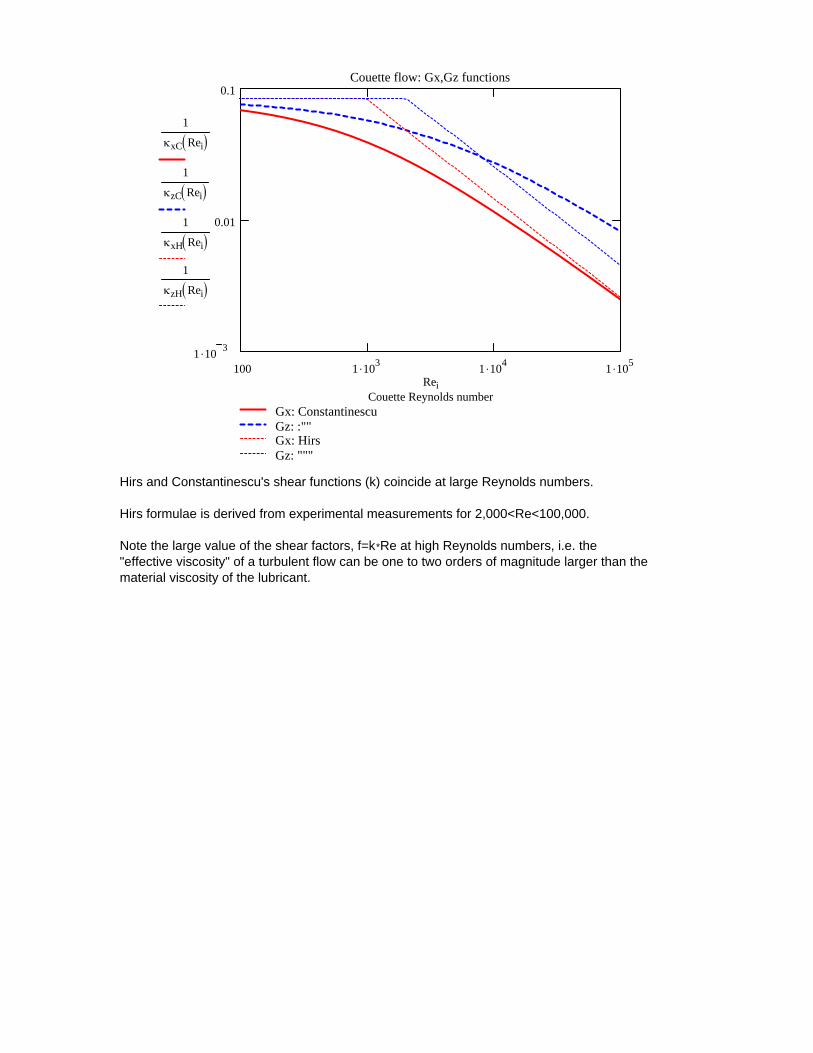
Gx: ConstantinescuGz: :""Gx: HirsGz: """

Couette flow: Gx,Gz functions


1

κxC Rei( )1

κzC Rei( )1

κxH Rei( )1

κzH Rei( )

Rei

Hirs and Constantinescu's shear functions (k) coincide at large Reynolds numbers.

Hirs formulae is derived from experimental measurements for 2,000<Re<100,000.

Note the large value of the shear factors, f=k*Re at high Reynolds numbers, i.e. the"effective viscosity" of a turbulent flow can be one to two orders of magnitude larger than thematerial viscosity of the lubricant.

1 .103 1 .104 1 .10510

100

1 .103

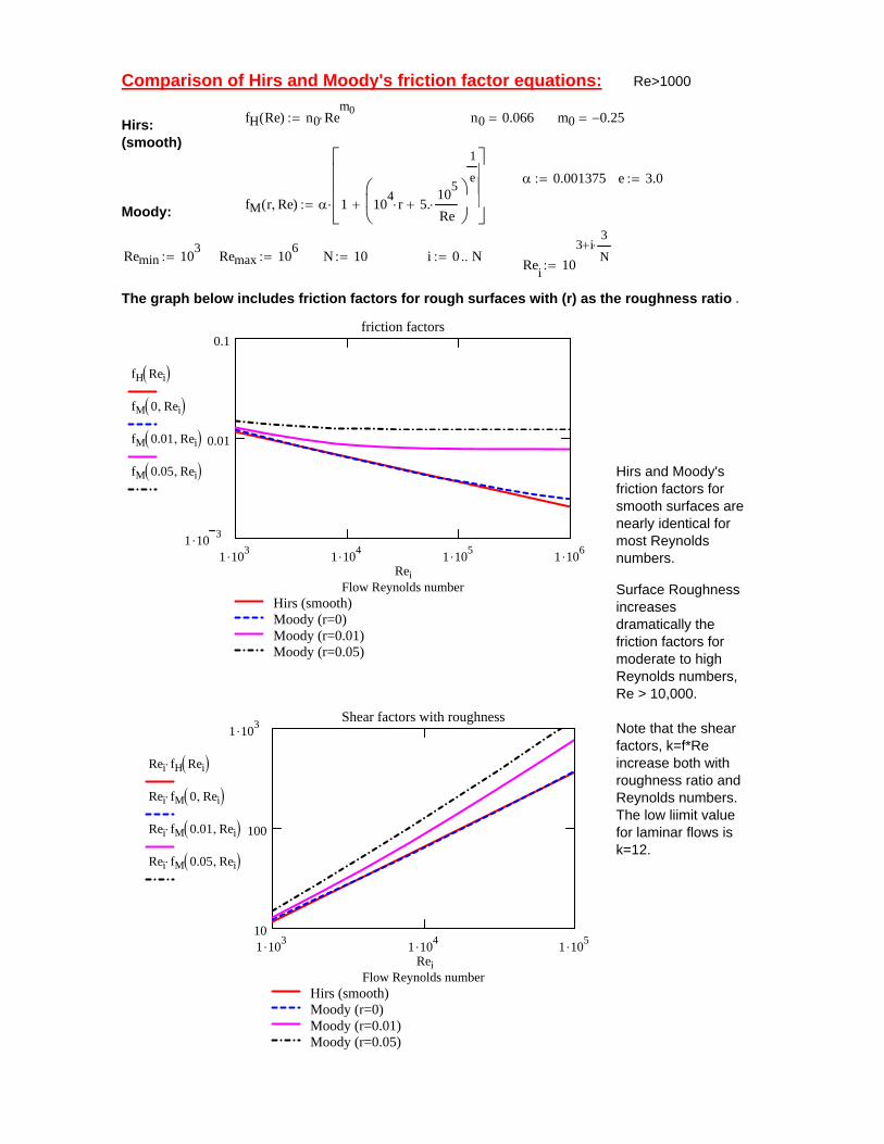
Hirs (smooth)Moody (r=0)Moody (r=0.01)Moody (r=0.05)

Shear factors with roughness

Flow Reynolds number

Rei fH Rei( )⋅

Rei fM 0 Rei,( )⋅

Rei fM 0.01 Rei,( )⋅

Rei fM 0.05 Rei,( )⋅

Rei

Hirs and Moody's friction factors for smooth surfaces are nearly identical for most Reynolds numbers.

Surface Roughness increases dramatically the friction factors for moderate to high Reynolds numbers, Re > 10,000.

Note that the shear factors, k=f*Re increase both with roughness ratio and Reynolds numbers.The low liimit value for laminar flows is k=12.

1 .103 1 .104 1 .105 1 .1061 .10 3

0.01

0.1

Hirs (smooth)Moody (r=0)Moody (r=0.01)Moody (r=0.05)

friction factors


fH Rei( )fM 0 Rei,( )fM 0.01 Rei,( )fM 0.05 Rei,( )

Rei

The graph below includes friction factors for rough surfaces with (r) as the roughness ratio .

Rei 103 i

3

N⋅+

:=i 0 N..:=N 10:=Remax 106

:=Remin 103:=

Moody: fM r Re,( ) α 1 104 r⋅ 5.105

Re⋅+

⎛⎜⎝

⎞⎟⎠

1

e

+

⎡⎢⎢⎢⎣

⎤⎥⎥⎥⎦

⋅:=

e 3.0:=α 0.001375:=

Hirs:(smooth)

m0 0.25−=n0 0.066=fH Re( ) n0 Rem0

⋅:=

Re>1000Comparison of Hirs and Moody's friction factor equations:

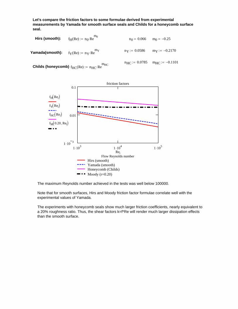
Let's compare the friction factors to some formulae derived from experimental measurements by Yamada for smooth surface seals and Childs for a honeycomb surface seal.

Hirs (smooth): fH Re( ) n0 Rem0

⋅:= n0 0.066= m0 0.25−=

nY 0.0586:= mY 0.2170−:=Yamada(smooth): fY Re( ) nY RemY

⋅:=

nHC 0.0785:= mHC 0.1101−:=Childs (honeycomb) fHC Re( ) nHC Re

mHC⋅:=

1 .103 1 .104 1 .1051 .10 3

0.01

0.1

Hirs (smooth)Yamada (smooth)Honeycomb (Childs)Moody (r=0.20)

friction factors


fH Rei( )fY Rei( )fHC Rei( )fM 0.20 Rei,( )

Rei

The maximum Reynolds number achieved in the tests was well below 100000.

Note that for smooth surfaces, Hirs and Moody friction factor formulae correlate well with the experimental values of Yamada.

The experiments with honeycomb seals show much larger friction coefficients, nearly equivalent to a 20% roughness ratio. Thus, the shear factors k=f*Re will render much larger dissipation effects than the smooth surface.

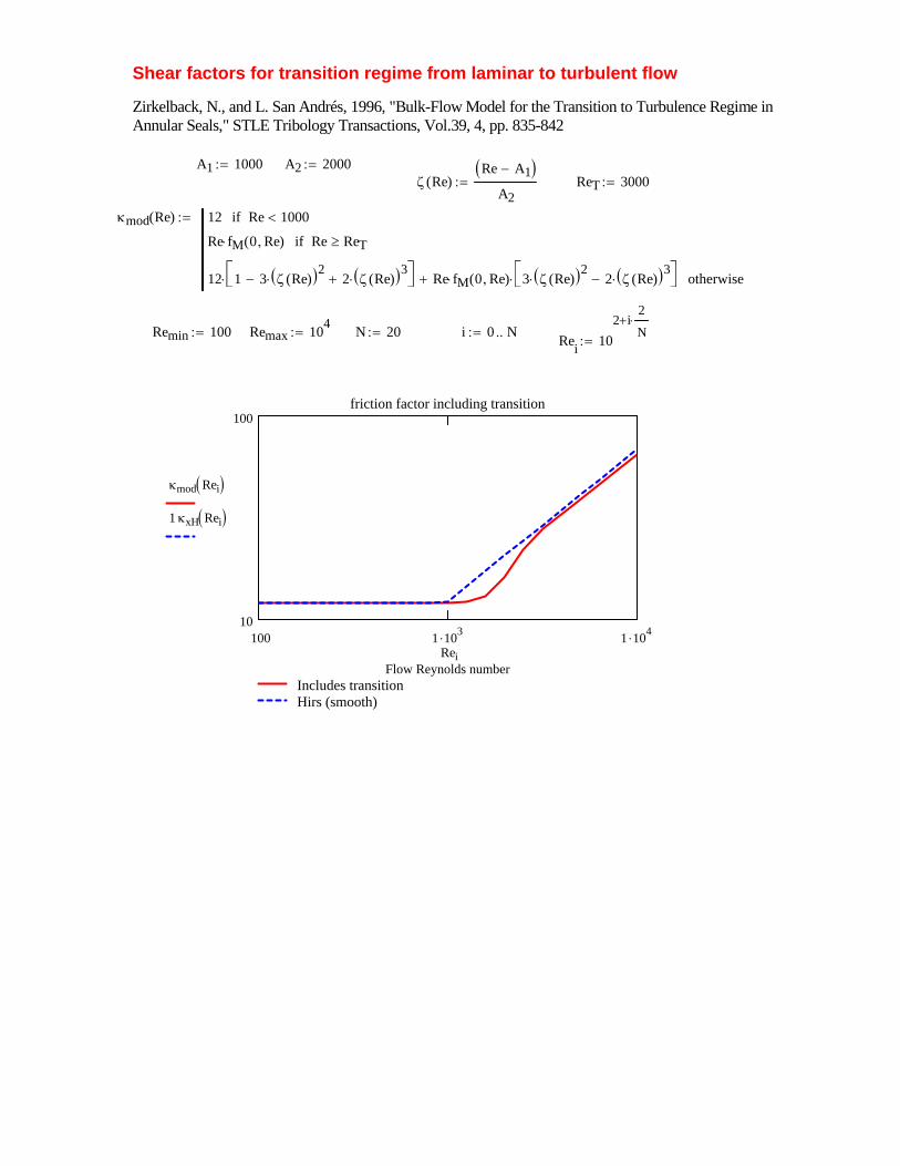
Shear factors for transition regime from laminar to turbulent flow

Zirkelback, N., and L. San Andrés, 1996, "Bulk-Flow Model for the Transition to Turbulence Regime in Annular Seals," STLE Tribology Transactions, Vol.39, 4, pp. 835-842

A1 1000:= A2 2000:=ζ Re( )

Re A1−( )A2

:= ReT 3000:=

κmod Re( ) 12 Re 1000<if

Re fM 0 Re,( )⋅ Re ReT≥if

12 1 3 ζ Re( )( )2⋅− 2 ζ Re( )( )3⋅+⎡⎣ ⎤⎦⋅ Re fM 0 Re,( )⋅ 3 ζ Re( )( )2⋅ 2 ζ Re( )( )3⋅−⎡⎣ ⎤⎦⋅+ otherwise

:=

Remin 100:= Remax 104:= N 20:= i 0 N..:= Rei 10

2 i2

N⋅+

:=

100 1 .103 1 .10410

100

Includes transitionHirs (smooth)

friction factor including transition


κmod Rei( )1 κxH Rei( )

Rei

notes 8. turbulence in thin film flows · notes 8. turbulence in thin film flows notes 8 detail the...

Documents