development of velocity dependent ice flexural …

DEVELOPMENT OF VELOCITY DEPENDENT ICE FLEXURAL

FAILURE MODEL AND APPLICATION TO SAFE SPEED

METHODOLOGY FOR POLAR SHIPS

By

© Mahmud Sharif Sazidy

A thesis submitted to the School of Graduate Studies

in partial fulfillment of the requirement for the degree of

Doctor of Philosophy

Faculty of Engineering and Applied Science

Memorial University of Newfoundland

April, 2015

St. John’s, Newfoundland, Canada

ii

ABSTRACT

The main focus of this research work is to develop a velocity dependent ice flexural

failure model through numerical investigation of ship icebreaking process. In addition,

the present work involves development of Excel-VBA software using this flexural failure

model to determine ice impact load, minimum plate thickness, frame dimensions and safe

speed methodology for Polar ships.

First of all, individual material models of ice crushing, ice flexure and water foundation

are developed using the FEM software package LS DYNA. Two different material

models of ice are used to represent the ice crushing and ice flexure. The input parameters

of these ice material models are selected from numerically conducted ice crushing test

and four point bending test. The water foundation effect is modeled using a simple linear

elastic material. The material models are incorporated into the numerical models of ship

icebreaking. Two collision scenarios are considered for the ship icebreaking models; a

head-on collision with a flat inclined ship face and a shoulder collision with an R-Class

ship. In these models, the rigid ship impacts a cantilever ice wedge. The ice wedge rests

on the water surface. Both collision scenarios are investigated with and without

considering radial cracks in the level ice.

The ice impact force and wedge breaking length are extracted from these numerical

models of ship ice wedge breaking. Results indicate that the ship velocity, normal ship

frame angle, ice wedge angle, ice thickness and radial crack significantly affect the

breaking process. At higher ship velocities, the bending crack location shifts toward the

iii

ice crushing zone and results in a higher impact force. Higher impact force is produced

for thicker ice, higher wedge angle and lower ship normal frame angle at a particular ship

velocity. The existence of radial cracks reduces the magnitude of impact force and

influences the breaking patterns.

A methodology is presented to estimate the dynamic ice failure load using existing static

failure models and dynamic amplification factors. The comparative study with these

dynamic failure loads indicates that the developed numerical model results are in good

agreement.

A flexural failure model is developed based on validated numerical model results. The

model provides velocity dependent force required to break an ice wedge in flexure. The

developed model is validated with full scale test data and with non-linear finite element

based dynamic bending model results. Application of this model is demonstrated to

estimate the limit bow impact load and design ice load parameters.

Finally, the Excel-VBA software “Safe Speed Check for Polar Ships” is developed using

the velocity dependent flexural failure model and Polar Rules based limit state equations.

This software and the velocity dependent flexural failure model are believed to help in

establishing a rational basis for safe speed methodology as well as in improving ship

structural standards and assessing ice management capability.

iv

ACKNOWLEDGEMENT

First and foremost, all praise to God, the most gracious and merciful who gave me the

opportunity and patience to carry out this research work.

I would like to express my sincerest gratitude to my academic supervisors, Dr. Claude

Daley, Dr. Bruce Colbourne and Dr. Amgad Hussein for their invaluable guidance,

supervisions and constant encouragement throughout this research work. Working with

them was a great learning experience and indeed without their assistance and support, this

thesis would not have been completed.

Sincere thanks to Sakib Mahmood, John Dolny, Bruce Quinton and Jungyong Wang for

their valuable suggestions and help during this work. I also greatly appreciate the

immeasurable co-operation and support from all the members of Sustainable Technology

for Polar Ships and Structures (STePS2) Research Project, Memorial University.

This investigation has been funded by Atlantic Canada Opportunities Agency, Research

and Development Corporation (RDC), American Bureau of Shipping (ABS), BMT Fleet

Technology, Husky Energy, Rolls-Royce Marine, Samsung Heavy Industries and the

National Research Council of Canada. I am grateful to them for their financial support.

I would like to extend my gratitude to my parents, wife, son, sisters and brothers for their

inspiration and motivation in my higher study.

v

TABLE OF CONTENTS

ABSTRACT……………………………………….……………………...........................ii

ACKNOWLEDGEMENTS……………………………………………………………....iv

TABLE OF CONTENTS………………………………………………………….............v

LIST OF TABLES…………………………………………………………………..........ix

LIST OF FIGURES……………………………………………………………………….x

LIST OF SYMBOLS………………………………………..……………………..……xix

Chapter 1 Introduction………………………………………………………………….1

1.1 Research Background………………...……………………………………...….1

1.2 Research Objectives and Scopes…………………………………………….......4

1.3 Thesis Organization……………………………………………………………..6

Chapter 2 Literature Review……………………………………………………………8

2.1 Introduction…………………………………………………………………...…8

2.2 Fundamentals of Ship-Ice Interaction...………………………………………..13

2.3 Modeling Efforts in Ship-Ice Interaction ……………………………………...21

2.3.1 Models using Analytical/Semi-Empirical Approaches ………………..23

2.3.2 Models using Advanced Numerical Techniques ……………………...36

2.4 Polar Ship Design Practice ……………………………………………………46

2.4.1 Polar Ice Classes ……………………………………………….……...47

2.4.2 Polar Design Load Scenario …………………………………….……..50

vi

2.4.3 Structural Limit State Analysis ………………………………………..56

2.5 Current Status of Safe Speed Methodology………………………..…………..58

2.6 Literature Summary and Problem Statement…………………………………..61

Chapter 3 Material Models for Ice and Water (in LS DYNA)………………………65

3.1 Introduction………………………………………………………………….…65

3.2 Ice Failure in Ship Icebreaking ………………………………………..………66

3.2.1 Ice Crushing Failure ……………………………………………...……67

3.2.2 Ice Flexural Failure…………………………………………………….69

3.2.3 Water Foundation Effect………………………………………….……70

3.3 Material Models for Ice and water ……………………………………………...71

3.3.1 Material Model for Ice Crushing………………………………………73

3.3.2 Material Model for Ice Flexure………………………………………...77

3.3.3 Material Model for Water Foundation………………...…………….…82

Chapter 4 Numerical Model of Ship Icebreaking…………………... …………….…88

4.1 Introduction………………………………………………………………….…88

4.2 Numerical Model of Ship Icebreaking ……………………………………...…89

4.2.1 Head-on Collision with Flat Inclined Face of Ship ………………...…89

4.2.1.1 Simple Ice Wedge Breaking………………………………...…90

4.2.1.2 Level Icebreaking (1500 Ice Wedge)………………………..…93

4.2.2 Shoulder Collision with R-Class Ship…………………………………94

vii

4.3 Model Results and Analysis ………………………………………………..…95

4.3.1 Simple Ice Wedge breaking in Head-on Collision ……………………95

4.3.2 Level Icebreaking in Head-on Collision ……………...…………...…105

4.3.3 Level Icebreaking in Shoulder Collision……………………………..110

4.4 Methodology to Formulate Dynamic Ice Load Models………………………111

4.5 Validation of Numerical Models………………………………………….…114

Chapter 5 Velocity Dependent Ice Flexural Failure Model…..……... …………….117

5.1 Introduction………………………………………………………………...…117

5.2 Velocity Dependent Flexural Failure Model ……………………………...…118

5.3 Comparison with Numerical Model ………………………………………….119

5.4 Validation with Full Scale Test Data …………………...…………………….123

5.5 Application to Bow Impact Load Estimation……………………………...…126

Chapter 6 Safe Speed Methodology for Polar Ships……………………………...…133

6.1 Introduction………………………………………………………………...…133

6.2 Design Ice Load Model ………………………………………………………134

6.3 Plate and Frame Design………………………………………………………139

6.4 Development of Safe Speed Methodology……………………………...……142

6.5 Safe Speed Check for Polar Ships-Software………………………………….146

Chapter 7 Summary and Recommendations………….. ………………………...…155

viii

7.1 Introduction………………………………………………………………...…155

7.2 Summary of Present Work……………………………………………………156

7.2.1 Study of Ship-Ice Interaction Process……………………………...…156

7.2.2 Material Models of Ice and Water………………………………...….158

7.2.3 Numerical Model of Ship Icebreaking…………………………..……159

7.2.4 Formulation of Dynamic Ice Load Models………………………...…160

7.2.5 Velocity Dependent Ice Flexural Failure Model…………………..…161

7.2.6 Safe Speed Methodology……………………………………………..162

7.3 Contributions of Present Work……………………………………………….162

7.4 Limitations of Present Work………………………………………………….166

7.5 Recommendations for Future Work………………………………………..…168

References ………………………………………………………………………..……169

Appendix A: LS DYNA Keyword File for Material Models………………….………183

Appendix B: LS DYNA Keyword File of Ship Ice Wedge Breaking…………………193

Appendix C: Data Sheet for Load Parameters, and Plating-Framing Particulars…..…197

ix

LIST OF TABLES

Table 2.1 Major ship classification societies/ rule systems and their ice classes…..46

Table 2.2 Description of IACS Polar ice classes………………………………...…48

Table 2.3 Parameters for pressure-area relationship in Polar Rules….………….…51

Table 2.4 Hull area factors in Polar Rules……………………………………….....55

Table 2.5 Peak pressure factor (PPF) in the Polar Rules………………………..….55

Table 3.1 Details of indenter in ice crushing test……………………………..……74

Table 3.2 Details of ice wedge in ice crushing test………………………………...74

Table 3.3 Details of ice beam in four point bending test…………………………...79

Table 3.4 Strain rates and compressive yield stress scale factors………………..…81

Table 3.5 Details of water foundation…………………………………………...…83

Table 4.1 Principal dimensions of ship……………………………………………..91

Table 5.1 Ice wedge geometry and landing craft bow particulars in full scale impact

test………………………………………………………………......…..124

Table 5.2 Ice crushing failure load model in IACS Polar Rules………………….127

Table 5.3 Principal particulars of ship and ice wedges for bow ice load……...….129

Table 6.1 Polar class dependent parameters for bow load calculation………..…..136

Table 6.2 Design load patch particulars in IACS Polar Rules…………………….138

Table 6.3 Minimum plate thickness for different framing configurations…….….140

Table 6.4 Limit state equations in Polar Rules for framing…………………...…..141

Table 6.5 Principal particulars of ship and structure for safe speed analysis……..143

Table 6.6 Design load patch parameters for PC 5, PC 6 and PC 7……………..…144

Table 6.7 Offered plate and frame dimensions for PC 5, PC 6 and PC 7…………145

x

LIST OF FIGURES

Figure 2.1 Damage events and damage severity in Canadian Arctic…………………9

Figure 2.2 Ice class ship damage a) Side damage of a tanker operated in Iqaluit,

Nunavut in 2004; b) Dents in the bow area of a chemical tanker operated

in Arctic Waters……………………………………………………….…12

Figure 2.3 Fundamental of ship-ice interaction indicating several mechanisms…....14

Figure 2.4 Local and global ice force on ice going ships………………………..….15

Figure 2.5 Ice force time history along with ice resistance………………………....15

Figure 2.6 Icebreaking pattern from a) Model test in Aalto ice tank ; b) Field

observation of YMER and c) Field observation of KV Svalbard………..17

Figure 2.7 Icebreaking pattern at three different ship speed…………………...……17

Figure 2.8 Icebreaking pattern from three different ship models indicating effect of

hull shape………………………………………………………………...18

Figure 2.9 Icebreaking pattern in thin ice (left) and thick ice (right)………………..18

Figure 2.10 Different icebreaking patterns idealized by a) Kashteljan; b) Enkvist; c)

Kotras and d) Riska……………………………………………………...19

Figure 2.11 Influence of edge crushing on icebreaking process…………………...…20

Figure 2.12 Influence of ship velocity and water foundation on icebreaking

process…………………………………………………………………....21

Figure 2.13 Kheisin extrusion model for ice-sphere interaction…………………...…26

Figure 2.14 Idealized level ice sheet on elastic foundation a) semi-infinite plate for

radial crack initiation and b) adjacent wedge-shaped beam for

xi

circumferential crack formation……………………………………….…29

Figure 2.15 Breaking phase in ship icebreaking model………………………………30

Figure 2.16 Circular contact detection technique in Sawamura’s models……………31

Figure 2.17 Contact geometries due to ice edge crushing in Sawamura’s models…...31

Figure 2.18 Contact detection technique in Su’s model……………………………....33

Figure 2.19 Ice wedge idealization and contact zone discretization………………….33

Figure 2.20 Geometries considered in contact area calculation………………………34

Figure 2.21 Modeling of bending crack initiation and propagation using different

numerical methods a) EEM; b) CEM; c) DEM and d) XFEM…………..37

Figure 2.22 Simulation results for ship (CCGS Terry Fox) in level ice [39] a)

advancing and b) turning at 10 m radius…………………………………38

Figure 2.23 Discrete element model of ship advancing through broken ice fields...…39

Figure 2.24 FEM model of ice wedge on water foundation along with edge boundary

condition and loading scenario……………………………………..……40

Figure 2.25 LNG ship-ice collision model (left) and ice edge crushing (right)……....41

Figure 2.26 Comparisons among Lagrangian, Eulerian and ALE solvers………...….43

Figure 2.27 Four point bending model in SPH method indicating bending crack…....44

Figure 2.28 Approximate comparisons between Baltic and Polar ice classes………..48

Figure 2.29 Ice strengthening requirements in Baltic ice rules……………………….49

Figure 2.30 Ice strengthening requirements in Polar ice rules……………………..…49

Figure 2.31 Polar Rules design scenario indicating ice edge crushing and ice

flexure……………………………………………………………………50

xii

Figure 2.32 Ice cusp geometry and contact condition in Daley and Kendrick’s flexural

failure model……………………………………………………………..52

Figure 2.33 Hull angle definition in Polar Rules…………………………………...…54

Figure 2.34 Peak pressure factor on structural member……………………………....56

Figure 2.35 Application of design load patch to structural member……………….....56

Figure 2.36 Plastic collapse mechanisms for plate limit state conditions…………….57

Figure 2.37 a) 1st limit state - 3 hinge formation in plastic frame; b) 2nd limit state -

shear panel formation in plastic frame and c) 3rd limit state - end shear in

plastic frame………………………………………………………….…..58

Figure 2.38 Concept of Russian ice passport………………………………………....60

Figure 2.39 CNIIMF ice certificate for Arctic Shuttle Tanker ……….……………....60

Figure 3.1 Fundamental ship icebreaking process……………………………...…...66

Figure 3.2 Indentation geometry of wedge-shaped ice for contact area calculation...68

Figure 3.3 Methodology and modeling approach in LS DYNA………………….....72

Figure 3.4 Geometric model of ice crushing test indicating indenter and short ice

wedge……………………………………………………………....…….73

Figure 3.5 Von-Mises stress distribution and change in crushing area……………...75

Figure 3.6 Normal impact force and contact area time histories in ice crushing test..75

Figure 3.7 Comparison between model and PC 1 pressure-area curves……….……76

Figure 3.8 Geometric model of four point bending test……………………….…….78

Figure 3.9 Relationship between compressive strength and strain rate……………..80

Figure 3.10 Bending failure of ice beam in four point bending test……………….....82

xiii

Figure 3.11 Force-time history in four point bending test…………………………....82

Figure 3.12 Geometric model of water foundation test for 0.5 m thick and 300 ice

wedge…………………………………………………………………….84

Figure 3.13 Interface pressure distribution for 0.5 m thick and 300 ice wedge…...…..85

Figure 3.14 Interface pressure distribution for 0.5 m thick and 600 ice wedge……….85

Figure 3.15 Pressure deflection curve for 0.5 m thick and 300 ice wedge …………...86

Figure 4.1 A rigid ship for ship icebreaking model……………………………...….90

Figure 4.2 Top view of ice wedge indicating ice crushing and bending zones……...91

Figure 4.3 Final model of ship ice wedge breaking process in head-on collision…..92

Figure 4.4 Ship level icebreaking in head-on collision indicating wedges separated

with duplicated nodes……………………………………………………94

Figure 4.5 Shoulder collision with R-Class ship…………………………………….95

Figure 4.6 a) Simple ice wedge breaking pattern (h=0.5 m, β'=650, θ= 300,

V=0.1 ms-1)………………………………..……………………..96

b) Simple ice wedge breaking pattern (h=0.5 m, β'=650, θ= 300,

V=0.5 ms-1)………………………………………………………96

c) Simple ice wedge breaking pattern (h=0.5 m, β'=650, θ= 300,

V=1.0 ms-1)……………………………………………………....97

d) Simple ice wedge breaking pattern (h=0.5 m, β'=650, θ= 300,

V=5.0 ms-1) …………………………………………………..….97

e) Simple ice wedge breaking pattern (h=0.5 m, β'=650, θ= 450,

V=0.1 ms-1)…………………………………………………...….98

xiv

f) Simple ice wedge breaking pattern (h=1.5 m, β’=650, θ= 300,

V=1.0 ms-1)…………………………………………………...….98

g) Simple ice wedge breaking pattern (h=0.5 m, β'=450, θ= 300,

V=0.5 ms-1)………………………………………………………99

Figure 4.7 a) Impact force vs time in simple ice wedge breaking (h=1.0 m,

β'=650, θ= 450, V=0.1 ms-1)………………………………....…..100

b) Impact force vs time in simple ice wedge breaking (h=1.0 m,

β'=650, θ= 450, V=1.0 ms-1)………………………………..……100

c) Impact force vs time in simple ice wedge breaking (h=1.0 m,

β'=650, θ= 450, V=5.0 ms-1)…………………………………….101

Figure 4.8 a) Impact force vs velocity in simple ice wedge breaking for different

ice thicknesses (β'=650, θ= 300)………………………….……..101

b) Failure time vs velocity in simple ice wedge breaking for different

ice thicknesses (β'=650, θ= 300)………………………..……….102

Figure 4.9 Impact force vs velocity in simple ice wedge breaking for different wedge

angles (h=0.5 m, β'=650)……………………………..…………………102

Figure 4.10 Impact force vs velocity in simple ice wedge breaking for different ship

angles (h=0.5 m, θ= 300)………………………………………………..103

Figure 4.11 a) Breaking length/ice thickness ratio vs velocity for different ice

thicknesses (β'=650, θ= 300)…………………………….………104

b) Breaking length vs velocity for different wedge angles (h=0.5 m,

β'=650)…………………………………………………..………104

xv

c) Breaking length vs velocity for different ship angles (h=0.5 m, θ=

300)………………………………………………….…………..105

Figure 4.12 a) Level icebreaking in head-on collision without radial cracks at 0.1

ms-1…………………………………………………………...…106

b) Level icebreaking in head-on collision without radial cracks at 1.0

ms-1…………………………………………………………...…106

c) Level icebreaking in head-on collision without radial cracks at 5.0

ms-1…………………………………………………………...…107

d) Level icebreaking in head-on collision with two radial cracks at 1.0

ms-1…………………………………………………………...…108

e) Level icebreaking in head-on collision with four radial cracks at

1.0 ms-1……………………………………………………….…108

f) Level icebreaking in head-on collision with four radial cracks at

5.0 ms-1…………………………………………………….....…109

Figure 4.13 Impact force vs ship velocity for level icebreaking in head-on

collision....................................................................................................109

Figure 4.14 a) Level icebreaking in shoulder collision without radial cracks at 1.0

ms-1………………………………...……………………………110

b) Level icebreaking in shoulder collision with four radial cracks at

1.0 ms-1…………………………...…..…………………………111

Figure 4.15 Comparison of bending failure loads in simple ship ice wedge breaking

(h= 0.5 m, θ=300, β'=550)………………………………………………115


(h= 1.0 m, θ=450, β'=650) )…………………………..…………………115


xvi

(h= 1.5 m, θ=600, β'=450) …………………………………...…………116

Figure 4.18 Comparison of ice wedge breaking lengths in different models………..116

Figure 5.1 Comparison of velocity dependent flexural failure model with numerical

model for ice wedge breaking in head-on collision at different ice

thicknesses (β'=650, θ=300)………………………………………...…..119


model for ice wedge breaking in head-on collision at different ice wedge

angles (h=0.5 m, β'=650)……………………………………………….120


model for ice wedge breaking in head-on collision at different normal ship

angles (h=0.5 m, θ=300) ………………………………………….…….120


model for ice wedge breaking in head-on collision with random breaking

parameters…………………………………………………………...….121


model for level icebreaking in head-on collision with and without radial

cracks………………………………………………………………...….121


model for level icebreaking in shoulder collision without radial

cracks……………………………………………………………………122


model for level icebreaking in shoulder collision with four radial

xvii

cracks…………………………………………………………………....122

Figure 5.8 Ice impact test arrangement indicating landing bow craft and ice wedge

shape [47]……………………………………………………………….123

Figure 5.9 Ice wedge geometry in full scale test (left), Varsta’s model (left) and

present model (right)………………………………………...………….125

Figure 5.10 Validation of velocity dependent ice flexural failure model with full scale

test data and Varsta’s model……………………………………………126

Figure 5.11 Ship velocity effect on bow impact load for an ice thickness of 1.5 m...130

Figure 5.12 Ship velocity effect on bow impact load at different ice thicknesses…..131

Figure 5.13 Ship velocity effect on bow impact load at different ship

displacements………………………………………………….………..132

Figure 6.1 Design ice load formulation methodology in Polar Rules…………..….134

Figure 6.2 Safe speed curve for PC 5 ship…………………………………………145



Figure 6.5 “Safe speed check for Polar ships” software……………………………147

Figure 6.6 Main features of “Safe speed check for Polar ships” software…………147

Figure 6.7 Ship and ice input parameters for ice load prediction…………………..148

Figure 6.8 Bow ice load prediction at a particular ice thickness and ship velocity...149

Figure 6.9 Investigation of ship velocity effect on bow ice load……………..……150

Figure 6.10 Ship velocity effect on ice crushing load at 1 m thick ice…………...…150

Figure 6.11 Ship velocity effect on ice flexural failure load at 1 m thick ice……….151

xviii

Figure 6.12 Ship velocity effect on limit bow impact load at 1 m thick ice……...….151

Figure 6.13 Velocity effect on ice crushing, flexural and bow ice load at 1 m thick

ice……………………………………………………………………….151

Figure 6.14 Ship velocity effect on bow impact load for ice thickness range of 1 m to 5

m (Sazidy model)……………………………………………………….152


m (Polar Rules model)………………………………………………….152

Figure 6.16 Plate and frame design for a 50,000 tones PC 5 ship…………………...153

Figure 6.17 Safe speed analysis for 50,000 tones PC 5 ship……………………...…154

Figure 6.18 Safe speed curve for 50,000 tones PC 5 ship………………………...…154

xix

LIST OF SYMBOLS

Af Flange area

Ao Minimum web area

An Nominal contact area

Aw Web area

ARi Load patch aspect ratio

b Patch load height

Cb Ship block coefficient

Cf,l,v.. Empirical parameters

Cm Ship mid-ship coefficient

Cpw Ship water plane coefficient

CFc Crushing class factor

CFD Patch class factor

CFDIS Displacement class factor

D Ship displacement

E Young modulus of ice

Ep Plastic hardening modulus

Ew Young modulus of water

ex Exponent in pressure-area relationship

fa Shape coefficient

Fc Ice crushing load

Fdf Dynamic ice load in flexural failure

xx

Ff /flex Flexural failure load of ice

Fi Bow impact load

Fl Limiting ice failure load

Fn Normal ice impact load

Fnd Dynamic normal impact load

Fvd Vertical component of dynamic ice load

FNd Dynamic Froude number

FNs Static Froude number

Fr Froude Number

h Ice thickness

kv Dynamic factor

kw Flange factor

KEe Effective kinetic energy

l Frame span

Lb Breaking length of ice

lc Characteristic length of ice

M Ship mass

Me Effective mass

Pavg Average contact pressure

Pf Bending failure load in Kashteljan’s model

Phs Hydrostatic pressure

Pi Load patch pressure

xxi

Plimit Limit load for framing

Po Nominal strength of ice

Qi Line load

s Frame spacing

t Plate thickness

V Velocity

vnrel Relative normal velocity between ship and ice

x Impact location

Zp Plastic modulus

α Waterline angles

β' Normal ship frame angles

θ Wedge angle of ice

ρ Density of ice

ρw Density of water

ϑ Vertical deflection of ice wedge

υ Poisson’s ratio

ζn Normal indentation

Ω Smallest angle between waterline and framing

σc Compressive strength of ice

σco Initial compressive strength

σf Flexural strength of ice

σmc Compressive mean stress

xxii

σmt Tensile mean stress

σto Initial tensile strength

σy Yield stress

ϵf Effective plastic failure strain

ϵp Effective plastic strain

1

Chapter 1

Introduction

1.1 Research Background

The Polar Regions, particularly the Arctic is believed to have vast amount of natural

resources. Industries are becoming more interested, and have increased their activities in

these regions. However, safe transportation of these resources in the Arctic is still a big

challenge. The heavy multi-year ice to thin first year ice poses a great risk to the ships

operating in these regions. In addition, these regions contain fish, wildlife and indigenous

people. Any accident in these regions could result a great economic loss and do potential

harm to the sensitive environment. Therefore, safety and sustainability are crucial for the

resource development and marine activities in these regions. Design of Ice Class ships is

an essential element in achieving this safety and sustainability. Historically, speed effects

have not been incorporated into calculations of structural loading from ice. The flexural

failure load model in the current IACS Polar Rules does not consider the velocity effects.

2

However, there is evidence that the ice failure load is influenced by the ship velocity due

to the presence of water foundation and ice inertia. Therefore, the flexural failure load

model could be improved to account for the velocity effects. In addition, the effect of

ship hull shape and ice condition on the icebreaking process needs to be considered.

At present, the idea of safe ship speed for operations in ice (Safe Speed Criterion) is a

topic of high priority at the International Maritime Organization (IMO) and with many

classification societies. Implicit in this interest is an understanding that ice loads are

speed dependent and that safe speed criteria can be a valuable tool for improving safety

as a methodology to provide an operational guidance to the Polar ships for safe

navigation through different ice conditions.

The development of a safe speed methodology requires structural limit state analysis and

ice impact load prediction that incorporates the effect of speed in the ice loading/failure

model. The structural limit state analysis is necessary to evaluate the strength of ship

structural components such as plates, frames etc. The IACS Polar Rules has well

established procedures and guidelines to determine these structural limit states. The most

challenging part of developing a safe speed methodology is a reliable prediction of ice

impact load. Physical model tests are of limited value in properly characterizing the local

ice impact forces. Model ice is normally aimed at replicating overall ice resistance rather

than the local contact pressures and forces. A good numerical or mathematical model can

focus on the local contact mechanics and be beneficial for this purpose.

3

However, development of an ice impact load model is complex. It requires adequate

knowledge of ship icebreaking process under dynamic loading conditions. To investigate

the ship icebreaking process; ice edge crushing, ice flexural failure and water foundation

effects need to be considered. Currently, there are few ice impact force models available

that can accurately describe all these aspects.

Proper numerical techniques and material properties of ice and water foundation are

important for modeling the ship icebreaking process. The ice is strain rate sensitive, and

responds differently in tension and compression. Hence, modeling of ice material is

difficult. It requires estimation of several physical and mechanical properties of ice.

Individual material properties are needed for the ice crushing and ice flexure behavior. In

addition, a material model of water is required to simulate the hydrodynamic force of

water foundation.

In level ice flexure, the formation of circumferential crack limits the maximum ice impact

force. Modeling of this crack initiation and propagation is difficult, and perhaps

computationally expensive. An efficient numerical technique needs to be introduced for

this purpose. In addition, the effect of radial cracks need to be considered in the modeling

of ship icebreaking.

This research work is intended to develop a velocity dependent ice flexural failure model

through the numerical investigation so that the model can be utilized to determine the

design ice load parameters, minimum plate thickness, frame dimensions, and safe speed

methodology for the Polar ships.

4

1.2 Research Objectives and Scopes

The primary objective of this research work is to develop a velocity dependent ice

flexural failure model in order to improve understanding of the effects of ship speed in

the load associated with icebreaking. This can provide a foundation to improve Polar ship

design practice and develop a safe speed methodology. Special emphasis is placed on

understanding and modeling aspects of the ship icebreaking and ice failure process to

accomplish this objective. Influencing factors such as ship velocity, ship hull shape, ice

conditions and water foundation are investigated in the present research. The Polar ship

structural limit state conditions have been reviewed and analyzed to establish the safe

speed methodology for the Polar ships. The objectives and scopes of this work can be

categorized as:

Review fundamental theories and modeling efforts of ship-ice interaction process

in order to identify the critical issues which are important to model and

investigate the ship icebreaking process.

Review Polar ship design practice and the current status of safe speed

methodology focusing on the bow impact load prediction, design ice load

parameter estimation, structural requirements, and safe speed methodology

formulation.

Develop numerical material models for ice crushing, ice flexure and water

foundation that incorporate the speed-dependent characteristics, based on

independent models of each process.

5

Develop a numerical model for the ship icebreaking to predict the ice flexural

failure by combining the individual process and material models. Investigate

dynamic ice flexural failure load models from existing static or quasi-static ice

load models and dynamic factor models. Validate numerical models using

dynamic flexural failure model.

Exercise the new model under various level icebreaking conditions to determine

the validity of the model and the assumptions of icebreaking mode. Use the model

to study ship velocity, hull shape, ice condition and water foundation effects on

the icebreaking process load in two different collision scenarios.

Formulate a velocity dependent ice flexural failure model based on numerical

model results. Validate the model using full scale test data and non-linear finite

element based dynamic bending model results.

Develop improved design ice load parameters, to design optimum plate and frame

dimensions, and to analyze the safe speed methodology based on application of

the velocity dependent ice flexural failure model.

Develop a convenient software tool to allow simple estimation of limit bow load,

design load parameters, minimum plate thickness, frame dimensions as well as

analysis of safe speed methodology for the Polar ships based on the analysis from

the velocity dependent ice flexural failure model.

6

1.3 Thesis Organization

The whole research work is organized in seven chapters. The first chapter addresses the

general background, objectives and scopes of the proposed research work.

Chapter 2 presents an overview of the existing literature which contributes to the current

research work. This includes review of current understanding in the ice failure and ship-

ice interaction process, ship-ice interaction modeling approaches, Polar ship design

practice and current status of safe speed criteria. At the end of this chapter, a literature

summary is presented to describe the motivation and methodology of this research work.

Chapter 3 addresses the development of material models for the ice crushing, ice flexural

failure and water foundation. A brief discussion on ice failure modes and water

foundation effect in the ship icebreaking process is also presented.

Chapter 4 presents the numerical models of ship icebreaking process considering two

collision scenarios and different breaking conditions. The effect of ship velocity over

icebreaking process is investigated for different ship hull shapes and ice conditions. A

methodology is also introduced in this chapter to develop the dynamic ice load models of

flexural failure from the existing analytical and semi-empirical models. Finally, the

numerical model results are validated against the developed dynamic ice load models.

Chapter 5 demonstrates a velocity dependent ice flexural failure model which is

developed based on the numerical model results. The model is validated against full scale

7

test data and non-linear finite element based dynamic bending model results. Application

of the model to investigate the ship velocity effect on bow impact load is illustrated with

an example Polar ship type (PC 1). A comparative study with respect to the IACS Polar

Rules is also presented for this investigation.

Chapter 6 involves the analysis of safe speed methodology for the Polar ships using the

velocity dependent flexural failure model. A brief overview on the design ice load model

formulation and structural requirements in the Polar Rules is presented. Examples are

illustrated for the Polar ships PC 5, PC 6 and PC 7 to determine the limit bow load,

design load patch parameters, minimum plate thickness, frame dimensions, and to

examine the safe speed capabilities in different ice conditions. Finally, the Excel-VBA

software is presented which allows the easy prediction of ice load, investigation of ship

velocity effect on ice load, optimum design of plate and frame, and analysis of safe speed

methodology for the Polar ships.

Chapter 7 summarizes and concludes the findings and limitations of the present work.

This chapter also includes the original contributions of this thesis along with some

guidelines for future work.

8

Chapter 2

Literature Review

2.1 Introduction

Historically, Arctic shipping was mainly limited to summer operation in ice free water or

light ice conditions. However increased marine activities in the region and decreasing ice

conditions are increasing the likliehood of year-round shipping operations through ice-

covered waters. According to the Arctic Council [1], year-round operation in ice-covered

water has been maintained since 1978/79 through the Northern Sea Route. The Council

reported that approximately 6000 vessels operated in the Arctic during a survey year

2004. More shipping activities are expected in the near future with increasing Arctic

natural resource development. However, the presence of ice is a major concern along

with other unique challenges for safe ship operation in this region.

9

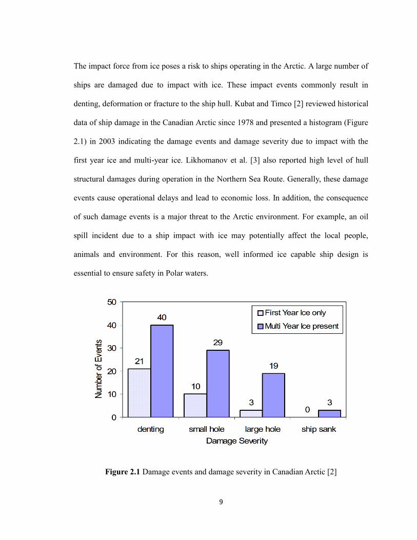
The impact force from ice poses a risk to ships operating in the Arctic. A large number of

ships are damaged due to impact with ice. These impact events commonly result in

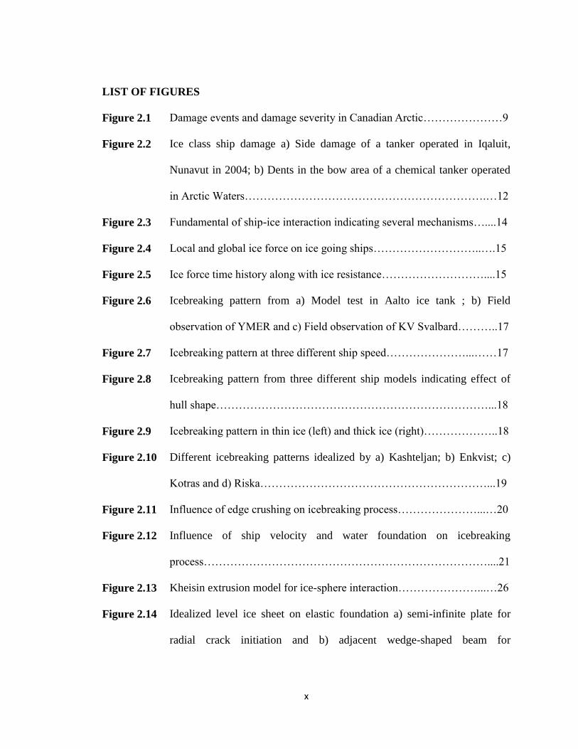
denting, deformation or fracture to the ship hull. Kubat and Timco [2] reviewed historical

data of ship damage in the Canadian Arctic since 1978 and presented a histogram (Figure

2.1) in 2003 indicating the damage events and damage severity due to impact with the

first year ice and multi-year ice. Likhomanov et al. [3] also reported high level of hull

structural damages during operation in the Northern Sea Route. Generally, these damage

events cause operational delays and lead to economic loss. In addition, the consequence

of such damage events is a major threat to the Arctic environment. For example, an oil

spill incident due to a ship impact with ice may potentially affect the local people,

animals and environment. For this reason, well informed ice capable ship design is

essential to ensure safety in Polar waters.

Figure 2.1 Damage events and damage severity in Canadian Arctic [2]

10

Polar ships or ice capable ships are designed to withstand ice loads without structural

failure. Hull structures are locally strengthened against high intensity ice pressure to

prevent the structural failure [3]. In general, this design or strengthening process involves

the determination of local impact load. This requires a clear understanding of the ship-ice

interaction process as well as the local contact mechanism between ship and ice.

Understanding the complete ship-ice interaction process is important to estimate the

global ice load, and hence to evaluate the overall performance of a ship in ice [4, 5]. On

the other hand, the local contact mechanism of ship icebreaking provides the local ice

load, and dictates the structural strengthening [4-6]. Therefore, the current understanding

of ship-ice interaction process focusing on the local contact mechanisms of ship

icebreaking is discussed in Section 2.2.

The International Maritime Organization (IMO), International Association of

Classification Societies Ltd. (IACS) and different classification societies have been

actively involved in developing rules and guidelines to design Polar ships and other ice

capable ships. Among these, the IACS Polar Rules (Polar UR) represent the latest

standard for Polar ship design [7]. In the Polar Rules, a glancing collision between the

ship and ice wedge is considered the design scenario to determine ice load parameters [7-

10]. This idealized glancing collision scenario involves a combination of ice crushing and

flexural failure modes [7-11]. The Polar Rules provide two individual ice failure models

to represent these ice crushing and ice flexural failure modes. The limiting bow impact

load from these two failure models is used to formulate the design ice load model [7, 9-

11

11]. The ice crushing failure model has been widely utilized to investigate the ship-ice

interaction at thicker ice or slow ship velocity operation [7, 12]. On the other hand, the

ice flexural failure model is a simple function of hull shape and ice conditions [7, 8, 10-

12]. Many researchers have pointed out that the Polar Rules based flexural failure model

ignores any velocity effects [7, 12]. Several studies indicate that ice inertia and the effect

of the water foundation make the ice flexural failure process strongly velocity dependent

[12-14]. This makes it difficult to extrapolate the PC design process to the cases of

thinner ice and higher ship velocity interaction. Surprisingly, few research studies have

been performed to improve this flexural failure model. For this reason, the present study

is focused on exploring the velocity dependency of ice flexural failure during the ship-ice

interaction. At present, analytical and numerical models are commonly utilized to

investigate this velocity dependency of ice flexural failure. A brief literature review is

presented in Section 2.3 to identify different modeling related issues to study the ship-ice

interaction process and velocity dependency of ice flexural failure.

The IACS Polar UR Rules provide a methodology to estimate the bow impact load [9,

10]. This impact load cannot be applied directly to the hull structure to evaluate the

structural strength [7, 8, 11]. The Polar Rules have specific formulas to transform this

bow impact load into a rectangular load patch which can be applied to the structure [7].

In addition, the Polar Rules contain limit state equations for ship plating and framing.

Both the load patch formulation and limit state equations are important for the Polar ship

design. Therefore, an overview on the Polar ship design practice is given in Section 2.4.

12

A Polar ship design or ice capable ship design does not ensure the safe ship operation in

the Arctic. Hull damage may take place in an ice class ship due to an accidental event or

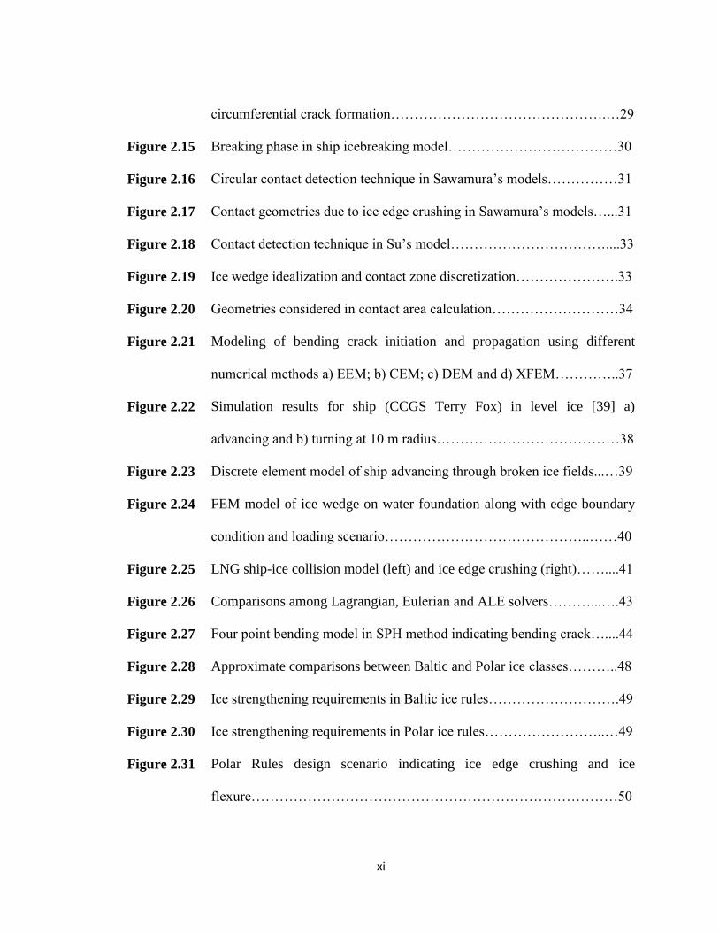
an extreme operational condition [15, 16]. Figures 2.2a and 2.2b are the indication of

such damages to the ice class ships operated in the Arctic.

Figure 2.2 Ice class ship damage a) Side damage of a tanker operated in Iqaluit, Nunavut

in 2004 [15]; b) Dents in the bow area of a chemical tanker operated in Arctic Waters [17]

Abraham [16] mentioned that the ice load acting on an Arctic ship is not constant and

may exceed the design limit. Ship velocity or interaction velocity greatly influences this

ice load [3]. For example, the peak ice load on a ship for a particular ice condition may

not be the same for slow velocity interaction and high velocity interaction. For the same

ship and ice condition, the slow velocity operation may be safe whereas the high velocity

operation may be unsafe. This implies that safe operation in the Arctic can be controlled

by regulating the ship velocity [7, 12]. A safe speed methodology can be an effective way

to regulate ship velocity in different ice conditions [7, 12]. Researchers and scientists

utilize several approaches and techniques to develop the safe speed methodology. Some

of these approaches and techniques are discussed in Section 2.5.

13

Based on the above discussion, the following four topics are identified as important in

developing a velocity dependent ice flexural failure model and safe speed methodology

for Polar ships:

Fundamentals of ship-ice interaction (Section 2.2)

Modeling efforts in ship-ice interaction (Section 2.3)

Polar ship design practice (Section 2.4)

Current status of safe speed methodology (Section 2.5)

Finally in Section 2.6, key information from the above topics is extracted and

summarized to explain the motivation and methodology of the present work.

2.2 Fundamentals of Ship-Ice Interaction

Designing an ice capable ship or developing a safe speed methodology for Polar ships

requires a clear understanding of the ship-ice interaction process. Significant effort has

been made to explore this complicated process [13, 14, 18]. Ship-ice interaction is a

complex process which involves several mechanisms and phases. Most studies idealize

these mechanisms and phases, and study each individually for complete understanding of

the interaction process. A schematic diagram of ship-ice interaction process is presented

in Figure 2.3 to illustrate these phases and mechanisms. In general, a localized interaction

process involves the breaking of an ice piece, rotation of the ice piece and sliding of the

ice piece etc. [13, 18-20].

14

Figure 2.3 Fundamental of ship-ice interaction indicating several mechanisms [19, 20]

The breaking phase initiates when the ship interacts with a part of the level ice sheet and

breaks off an ice piece. This breaking phase is associated with deformation, crushing,

bending and fracture of ice. In a second phase, the broken ice piece is rotated or turned

until it is parallel to the ship hull [18]. Finally, the rotated ice piece slides along the hull

and clears out from the ship path. Detailed description of the interaction process can be

found in Liu [21], Aksens [18], Daley and Colbourne [6] and Su et al. [14].

During ship-ice interaction, ice loads acting on the ship can be categorized as global ice

load and local ice load as shown in Figure 2.4. Each and every individual local ice

interaction mechanism contributes to the global ice load. Individual phases of the

interaction process provide the local ice loads. Several approaches and approximations

are made to determine the global ice load and local ice load. In general, local load

15

components from individual phases and mechanisms are integrated to obtain the global

ice load and ice resistance. Su et al. [14] presented an idealized time history of the ice

force from each mechanism, and provided definition of the ice resistance or global ice

force as shown in Figure 2.5.

Figure 2.4 Local and global ice force on ice going ships [19]

Figure 2.5 Ice force time history along with ice resistance [14]

16

The above figure indicates that the local ice load reaches at a maximum value in the

breaking phase when the ice fails in flexure or bending. Similarly the global load

fluctuates as the sum and average of the local loads rise and fall. Thus both the local and

global maximum ice load is higher than the corresponding average value. The ice

resistance and global ice load are important for evaluating the overall performance of

ship in ice but do not generally pose structural risk [4, 12]. Structural risk arises from the

local peak loads. Therefore, it is essential to investigate the local contact mechanism

involved in the ship icebreaking phase to predict this peak load.

Most of the existing literature focuses on the determination of the resistance force and the

maneuvering forces [13, 14, 18, 20-25]. In those cases, only the critical information is

extracted which is relevant to the icebreaking phase. The following discussions will focus

on the icebreaking pattern during ship-ice interaction.

During the ship-ice interaction, the resulting icebreaking pattern is irregular and difficult

to predict [21]. According to Liu [21], non-uniformity of the mechanical properties of ice

is the main reason for this irregular behavior. Significant effort has been made to study

this irregular icebreaking pattern through model tests and field trials. Figure 2.6 is the

example of such icebreaking patterns from model tests and field trials. The figure

indicates the formation of several ice wedges. These ice wedges are the result of radial

and circumferential cracks in the ice sheet. Several factors such as ship geometry, ship

velocity, and ice condition affect this crack initiation and propagation process, and hence

influence the icebreaking pattern. Myland and Ehlers [26] have investigated the effect of

17

such influencing factors. Figures 2.7 to 2.9 indicate how ship velocity, ship hull shape

and ice condition affect the icebreaking pattern.

Figure 2.6 Icebreaking pattern from a) Model test in Aalto ice tank [27]; b) Field

observation of YMER [27, 28] and c) Field observation of KV Svalbard [13]

Figure 2.7 Icebreaking pattern at three different ship speed [26]

18

Figure 2.8 Icebreaking pattern from three different ship models indicating effect of hull

shape [26]

Figure 2.9 Icebreaking pattern in thin ice (left) and thick ice (right) [26]

The above study and observation are not sufficient to characterize the icebreaking process.

Liu [21] mentioned that there is no universally accepted icebreaking model available due

to the complexity involved in the process. However, many researchers idealize the

icebreaking process based on field observation or model scale tests. Some of the idealized

icebreaking patterns are shown in Figure 2.10.

19

(a)

(b)

(c)

(d)

Figure 2.10 Different icebreaking patterns idealized by a) Kashteljan [29];

b) Enkvist [29]; c) Kotras [31] and d) Riska [20]

The above idealized breaking patterns are the indication of ice wedge formation as well.

Lu et al. [33] mentioned that the radial cracks appear first and separate the ice sheet into

several wedges during the ship-ice interaction. The ice wedges finally fail

circumferentially in flexure. According to Lubbad and Loset [13], 3 to 5 ice wedges form

during this interaction process. Therefore, many researchers have investigated the

breaking process of simple ice wedge instead of full ice sheet [13, 33-35].

20

Simple ship ice wedge breaking analysis is sufficient to extract the local contact force.

This type of analysis is simple but provides information regarding the local contact

mechanism. In the IACS Polar Rules, the design ice load parameters are also estimated

based on the ship and ice wedge (150 deg) breaking [7-9, 12]. It is important to consider

both the ice edge crushing and ice flexural behavior in the ice wedge breaking analysis.

Daley and Colbourne [6] mentioned that the ice edge must first be crushed in order to

develop enough force to achieve this flexural failure. The influence of edge crushing on

the ice load is illustrated in Figure 2.11. Without edge crushing the magnitude of

maximum ice force may not be changed but it will influence the load duration and

average force value [6]. Perhaps, the edge crushing can be ignored in the analytical or

mathematical analysis if appropriate idealizations and assumptions are made. For

example, Aksnes [18] assumed that the ice sheet bent and deflected until the flexural

failure occurred for an analytical model of moored ship and ice interaction. Crushing was

not considered in that model. However, the edge crushing needs to be considered for

physical or numerical modeling in order to simulate the proper bending response. Su et al.

[14] and Tan et al. [28] emphasized on the importance of considering edge crushing in

the ship-ice interaction modeling.

Figure 2.11 Influence of edge crushing on icebreaking process [6, 36]

21

In the ship ice wedge breaking analysis, impact force and wedge breaking length are

evaluated to achieve the proper bending response. This impact force and breaking length

strongly depend on the hull geometry, ice conditions, ship velocity and the presence of

the elastic water foundation [13, 18, 26, 36]. For low velocity interactions, such as a

moored ship or an offshore structure, the velocity effect or dynamic effect can be

neglected [13, 18]. However, both the velocity and water foundation effects are

significant for a ship with normal or high operating velocity. Daley and Colbourne [6]

explained the velocity dependency of icebreaking process. The ice wedge is accelerated

and the hydrodynamic force from the water foundation is changed, as the ship advances.

Figure 2.12 indicates a velocity dependency in the icebreaking process due to the water

foundation and ice inertia.

Figure 2.12 Influence of ship velocity and water foundation on icebreaking process [6]

2.3 Modeling Efforts in Ship-Ice Interaction

Model scale and full scale tests are thought to be the most accurate and acceptable

methods for investigating the ship-ice interaction process. These provide useful

information about the phenomena observed during ship-ice interaction [37]. The major

22

challenge of model and full scale tests is that they cannot explain all the complexities

involved in the interaction process. Moreover, model scale tests are expensive and

imperfect, while full scale tests are even more expensive and uncontrolled [6].

Nowadays, numerical modeling is preferred over the model and full scale tests to

investigate the ship-ice interaction process. Numerical modeling is cost-effective and

provides detailed information that cannot be obtained from those tests, for example

pressure distribution, stress states etc. [5, 37].

Ship-ice interaction models can be studied analytically or numerically. These models are

developed based on the observation of ship-ice interaction process and ice failure process

[38]. Different characterizations and idealizations of the processes have been made in the

recent past to obtain a reliable ship-ice interaction model, yet no universally accepted

analytical or numerical model is found in the literature [39]. This is due to the

complexities associated with the ship-ice interaction and uncertainties involved in the ice

failure process [39, 40].

In this study, the considered ship-ice interaction models are categorized based on their

formulation methods. The first category includes models based on analytical or semi-

empirical approaches. The second category consists of models with advanced numerical

techniques such as Finite Element Method (FEM), Discrete Element Method (DEM),

Cohesive Element Method (CEM) etc. Discussions on each and individual modeling

aspect of both categories are out of scope for the present study. General discussions on

23

existing models are presented in Sub-sections 2.3.1 and 2.3.2. However, the following

critical areas are emphasized:

Contact between ship and ice, pressure-area relationship

Interaction between ice and water foundation

Icebreaking pattern, breaking force and breaking length

Ice behavior and failure process

Influencing parameters of ship icebreaking process

Dynamic effect of ice inertia and water foundation

Modeling techniques and approaches

Material models of ice and water foundation

2.3.1 Models using Analytical/Semi-Empirical Approaches

Modeling of the ship-ice interaction or ice-structure interaction is not new. According to

Jones [41], the first scientific article on icebreakers was published by Runeberg [42] in

1888/89, which was the only published article in 19th Century. The article provided

several expressions for continuous icebreaking to calculate the vertical pressure at the

bow, the broken ice thickness and total elevation at the fore-end. Runeberg’s [42] work

recognized the importance of hull-ice friction effect on the ice resistance and stem angle

effect on the bow. The work suggested that the vertical force component should be as

large as possible to break the ice. This is still maintained in modern icebreaker design by

sloping the bow at the waterline [41].

24

The vast majority of the work on ship performance in ice has been carried out since the

1960s. In 1968, Kashteljan et al. [29] analyzed the details of level ice resistance [21, 29,

41]. In their analysis, the total ice resistance was divided into four components; resistance

due to icebreaking, resistance due to forces related with submersion of broken ice,

turning of broken ice, change in position of icebreaker and dry friction, resistance due to

passage through broken ice, and resistance due to water friction and wave making [29,

41]. Kashteljan’s work established a platform based on dividing the problem into

mechnasms or components for further research on different aspects of ship ice resistance

and ship-ice interaction process.

The strategy of Kashteljan et al. [29] has been followed by many researchers in which the

total resistance force is a summation of several force components. In most of these cases,

individual phases and mechanisms of the ship-ice interaction process are investigated

separately and incorporated into a final resistance formula. For example, Lewis and

Edwards [43] gave an ice resistance formula in 1970 through detailed analysis of full-

scale and model scale data for the icebreaker Wind-class, Raritan, M-9 and M-15. The

formula consisted of individual force components to represent the icebreaking and

friction, ice buoyancy, and momentum change between the ship and broken ice [41]. In

the same year, White [44] provided a purely analytical method to investigate the bow

performance in continuous icebreaking, ramming and testing extraction ability. Based on

this investigation, a blunter bow form was recommended for the Polar ship which was

used in the design of the MV Manhattan for its operation in the Arctic [41]. Later in

25

1972, Enkvist [30] made a significant contribution in the literature of ship-ice interaction.

A semi-empirical ice resistance formula was derived from the combination of analytical

analysis, non-dimensional analysis, model scale test and limited full scale test data [30,

41]. The velocity dependent term and the ice submergence term in the formula were

isolated through model tests and pre-sawn tests, respectively [41].

In 1973, Milano [45] provided a purely analytical model to evaluate the ice resistance

based on energy needed for a ship to move through the level ice [41]. Milano [45] also

followed a non-dimensional approach, similar to Lewis and Edwards [43], to develop a

design chart which was further utilized to predict the total ice resistance for different

icebreakers.

One of the earliest ice interaction models is the Kheisin’s extrusion model [46]. The

model was developed in 1975 based on a drop test of steel ball on ice cover. The concept

of pulverized layer formation at the ice-sphere contact interface was introduced into the

model (Figure 2.13). The pulverized layer of uniform thickness must have to be extruded

when the ice is crushed. The pulverized layer thickness was assumed as proportional to

the local pressure. This assumption enabled the model to predict the ice pressure, ice

force and indenter velocity which were unmeasurable previously [6, 38]. This simplified

model has been used as a crushing model for many years [6]. The model cannot explain

all the aspects of the interaction process.

26

Figure 2.13 Kheisin extrusion model for ice-sphere interaction [6, 46]

In 1983, Varsta [47] adopted Kheisin’s extrusion model into his ice load model to explain

the wet contact between the ship and ice [38]. For the dry contact, Varsta [47] developed

a new model using the finite element analysis and the Tsa-Wu failure criteria [38].

In 1989, Lindqvist’s [36] ice resistance model considered three individual mechanisms;

ice crushing at the stem, ice bending over the whole bow and ice submergence along the

ship hull [6, 21]. The force components from each individual mechanism were derived

analytically. These force components were combined to obtain the total ice resistance on

a ship. This model also accounted for the velocity effect on the ice resistance through

empirical formulas. According to Liu [21], these empirical formulas are over simplified

and need further refinement. Nevertheless, the model is helpful to understand the

interaction process, and can be useful in the early ship design process. The Lindqvist’s

model has been used to predict the ice resistance for several icebreakers such as Jelppari,

Otso, Vladivostok, Mergus, Ware, Valpas and Silma etc. [21].

27

The early models mentioned above are purely analytical or semi-empirical, and are

applicable to either static problems or simple contact geometry cases. Most of these

models may not capture the entire phenomenon of ship-ice interaction process, yet each

has a contribution to the current state of interaction modeling practice. Some of these

models are still being used. For example, Valanto [48] utilized Lindqvist’s [36] semi-

empirical model for the underwater components, and combined it with a 3D numerical

model of ship icebreaking for the prediction of ice resistance. A number of numerical

models were developed in the recent past using these analytical or semi-empirical

approaches for the real time simulation of continuous ship icebreaking. Most of these

models utilize the analytical or semi-empirical formulas which were numerically

integrated [13, 14, 21]. Liu’s [21, 49] ice-hull interaction model is an example of this

approach for the real-time simulation of ship maneuvering in level ice. Liu [21, 49]

utilized Kotras’s [31] idealized icebreaking pattern mentioned in Figure 2.10c to

determine the depth and width of ice cusps. The model consisted of breaking, buoyancy

and clearing phases. The breaking phase was comprised of ice crushing and bending

failure. In ice crushing failure, the impact load (Fn) normal to the contact interface was

related to the compressive strength (σc) of ice and the nominal contact area (An) with the

following formula:

𝐹𝑛 = 𝜎𝑐𝐴𝑛 (2.1)

This crushing formula had been widely utilized in many crushing related studies [14, 24,

27, 28]. In Liu’s model, the compressive strength or pressure was assumed as constant

28

over the contact area, which is a simplification of the real case. There is much evidence

that the pressure changes with the contact area, and significantly affects the crushing

force component [4, 50].

The bending failure load (Pf) was calculated using Kashteljan’s semi-empirical formula

given in Kerr [51]. The formula was based on the bearing capacity of a floating ice sheet

subjected to the static or quasi-static load. This failure load was expressed as a simple

function of the ice flexural strength (σf), ice wedge angle (θ) and ice thickness (h) as

shown below:

𝑃𝑓 = 𝐶𝑓 (𝜃

𝜋)2

𝜎𝑓ℎ

(2.2)

The empirical parameter (Cf) in the equation can be tuned to match experimental results.

This bending formula does not account for any dynamic effect in the interaction, and is

suited for the static loading conditions only. Additionally, it does not incorporate

information regarding the hull geometry effect on the bending load. However, this

bending model is commonly used by many researchers because few alternative bending

formulas [5, 14, 24, 27, 28, 52] are available.

Lubbad and Loset [13] developed another numerical model for real time simulation of

ship-ice interaction. Equations of motion for a rigid ship in three degree of freedom

(DOF) were integrated over time. The ice was assumed a homogeneous, isotropic elastic-

brittle material. Their work included investigation of radial crack initiation as well as the

29

circumferential crack formation. For anticipating the radial crack initiation, a closed form

analytical solution of bending stress was derived based on the idealized semi-infinite

plate resting on an elastic foundation which was subjected to a uniformly distributed load.

This idealized semi-infinite plate was replaced with the adjacent wedge-shaped ice beam

to predict the wedge failure and the formation of the circumferential crack. Nevel [60]

provided power series solution was used for this prediction. Figure 2.14 indicates these

two idealizations of an ice sheet resting on a water foundation.

Figure 2.14 Idealized level ice sheet on elastic foundation [13] a) semi-infinite plate for

radial crack initiation and b) adjacent wedge-shaped beam for circumferential crack

formation

Lubbad and Loset’s [13] model ignored the edge crushing and considered only the

bending failure for icebreaking phase. The authors discussed the dynamic effect of ice

inertia and water foundation on the breaking force and the breaking length. However, the

dynamic effect was not considered in the model.

30

Sawamura et al. [5] developed a numerical model for the repetitive ship icebreaking

pattern. The model considered the breaking phase, consisting of crushing and bending of

an ice beam as shown in Figure 2.15. The model ignored the rotation and sliding phases

as these are not important for the breaking force estimation. A circular contact detection

technique was applied to determine the contact point between the ship and ice edge

(Figure 2.16). The crushing formula given in Eq. (2.1) was used in the model. The

compressive strength was constant in the model. The model adopted two different contact

areas based on the crushing edge geometry as shown in Figure 2.17. The triangular

contact area was generated because of the crushing on the top corner of the ice edge.

Whereas, a rectangular contact area resulted when the crushing reached the bottom corner

of the ice edge. Sawamura et al. [5] derived contact area formulas based on these contact

geometries. Later Sawamura et al. [35] adopted FEM results from the fluid-ice interaction

analysis into the model to represent the dynamic bending failure of ice sheet. The fluid-

ice interaction analysis assumed that the bending failure occurs when the maximum

bending stress exceeds the flexural strength of ice.

Figure 2.15 Breaking phase in ship icebreaking model [5]

31

Figure 2.16 Circular contact detection technique in Sawamura’s models [5]

Figure 2.17 Contact geometries due to ice edge crushing in Sawamura’s models [5]

32

The ship icebreaking model of Sawamura et al. [5] was extended in Sawamura et al. [53]

for the ship maneuvering application in the level ice. The model considered 3 DOF rigid

body motions of ship in surge sway and yaw directions. The crushing force component

was modified by including a friction force component. The breaking pattern of the ice

cusp was assumed as a circular arc. Sawamura et al.’s [5, 53] models identified the basic

mechanisms which are crucial to model the dynamic ship icebreaking process. However,

these simplified models need further improvement to determine more accurate crushing

and bending force components.

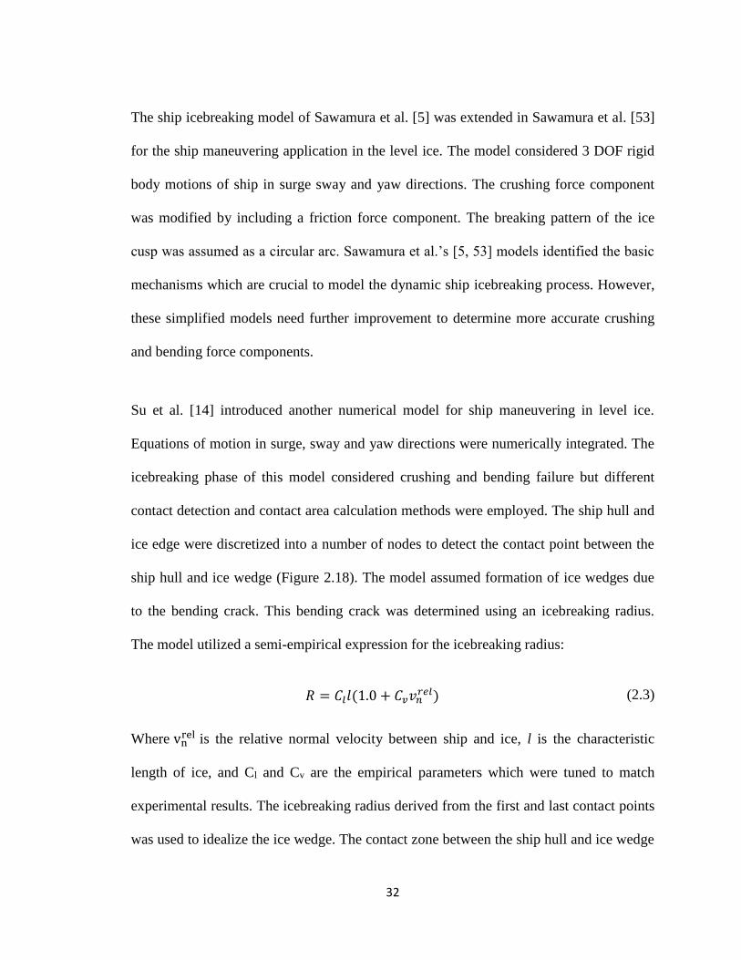
Su et al. [14] introduced another numerical model for ship maneuvering in level ice.

Equations of motion in surge, sway and yaw directions were numerically integrated. The

icebreaking phase of this model considered crushing and bending failure but different

contact detection and contact area calculation methods were employed. The ship hull and

ice edge were discretized into a number of nodes to detect the contact point between the

ship hull and ice wedge (Figure 2.18). The model assumed formation of ice wedges due

to the bending crack. This bending crack was determined using an icebreaking radius.

The model utilized a semi-empirical expression for the icebreaking radius:

𝑅 = 𝐶𝑙𝑙(1.0 + 𝐶𝑣𝑣𝑛𝑟𝑒𝑙) (2.3)

Where vnrel is the relative normal velocity between ship and ice, l is the characteristic

length of ice, and Cl and Cv are the empirical parameters which were tuned to match

experimental results. The icebreaking radius derived from the first and last contact points

was used to idealize the ice wedge. The contact zone between the ship hull and ice wedge

33

was further discretized into a number of triangles for calculating the contact area. Figure

2.19 indicates the ice wedge idealization and contact zone discretization process. This

model also considered two ice edge crushing scenarios (Figure 2.20) to derive the contact

area equations.

Figure 2.18 Contact detection technique in Su’s model [14]

Figure 2.19 Ice wedge idealization and contact zone discretization [14]

34

Figure 2.20 Geometries considered in contact area calculation [14]

The normal contact force in Su et al.’s [14] model accounted for the friction and ship

velocity. The contact force was further resolved into horizontal and vertical components.

The vertical component of contact force caused the bending failure of the ice wedge. This

model used Kashteljan’s model, mentioned in Eq. (2.2), to predict the flexural failure

which ignores the dynamic effect.

Su et al.’s [14] modeling approach was followed by Zhou et al. [52], and was improved

by Tan et al. [24, 27, 28] for several ship-ice interaction problems. Zhou et al. [52]

utilized Su et al.’s numerical approach for modeling the dynamic ice force on a moored

icebreaking tanker. Tan et al. [24] extended Su et al.’s model from the 3 DOF to 6 DOF

ship motions. One of the major drawbacks with these models is the assumption of

constant contact pressure. Tan et al. [28] improved the model by introducing the

pressure-area relationship in the local contact force calculation. The model was further

improved by Tan et al. [27] to include the dynamic effect in flexural failure. For this

purpose, Kashteljan’s bending model was modified with a semi-empirical dynamic

35

factor. The dynamic factor is a function of normal ship velocity (v), and was established

based on finite element analysis results and physical tests. This allowed investigation of

velocity effect on the icebreaking process. The dynamic bending failure model used by

Tan et al. [27] can be written in SI units:

𝑃𝑓 = (1.65 + 2.47𝑣0.4)𝜎𝑓ℎ2 (𝜃

𝜋)2

(2.4)

Aksnes [18] presented a simple one-dimensional (1D) numerical model to analyze the

interaction between a moored ship and drifting level ice. The ship motion in the surge

direction was considered, and the ice properties were sampled from probability

distributions. The total force on the ship was taken as the sum of the hydrodynamic force,

mooring force and ice force. The ice force was divided into a penetration dependent

breaking term and a velocity dependent term. Again, the breaking term was associated

with the icebreaking, rotation and sliding phases. The breaking force was derived based

on the semi-infinite plate on elastic foundation, but neglected the dynamic effects of

beam and foundation. A deflection based failure criteria was assigned to the breaking

phase, and ignored any edge crushing. The velocity effect was accounted by considering

the damping from ice as a function of relative velocity between the ship and ice. The

model is applicable to the low ice drift velocity interaction problems and limited to

moored ships only.

The above mentioned numerical models are helpful to understand the ship icebreaking

process. These are beneficial to predict the global ice force or ice resistance for the

continuous icebreaking and ship maneuvering. Most of these are applicable to simplified

36

cases and avoid many important features. These models are not capable of simulating the

bending crack initiation and propagation effectively.

2.3.2 Models using Advanced Numerical Techniques

With the advancement of computational technology, several numerical methods and

techniques, such as Finite Element Method (FEM) with several integration schemes,

Element Erosion Method (EEM), Discrete Element Method (DEM), Cohesive Element

Method (CEM), Extended Finite Element Method (XFEM), and Element Free Gelerkin

Method (EFGM) are available for ship-ice interaction modeling [33, 35, 54-59]. These

methods are well suited to investigate the non-linear problems as they allow modeling of

material failure process or simulating transition from continua to discontinua [33]. These

methods are effectively employed to simulate ice behavior under dynamic conditions and

to capture the ice bending crack initiation-propagation [33, 57, 59]. Several, software

packages such as ABAQUS/Explicit, LS DYNA, ANSYS, DECICE, DYTRAN etc. are

able to implement most of the numerical methods listed above. Proper software package

and numerical methods are selected based on problem nature, desired computational

efficiency and desired accuracy of results.

Lu et al. [33], and Daiyan and Sand [59] examined several numerical methods, such as

the element erosion method, the cohesive element method, the discrete element method,

and the extended finite element method, for ice bending models. These numerical

methods were used to simulate an ice wedge-conical structure interaction scenario using

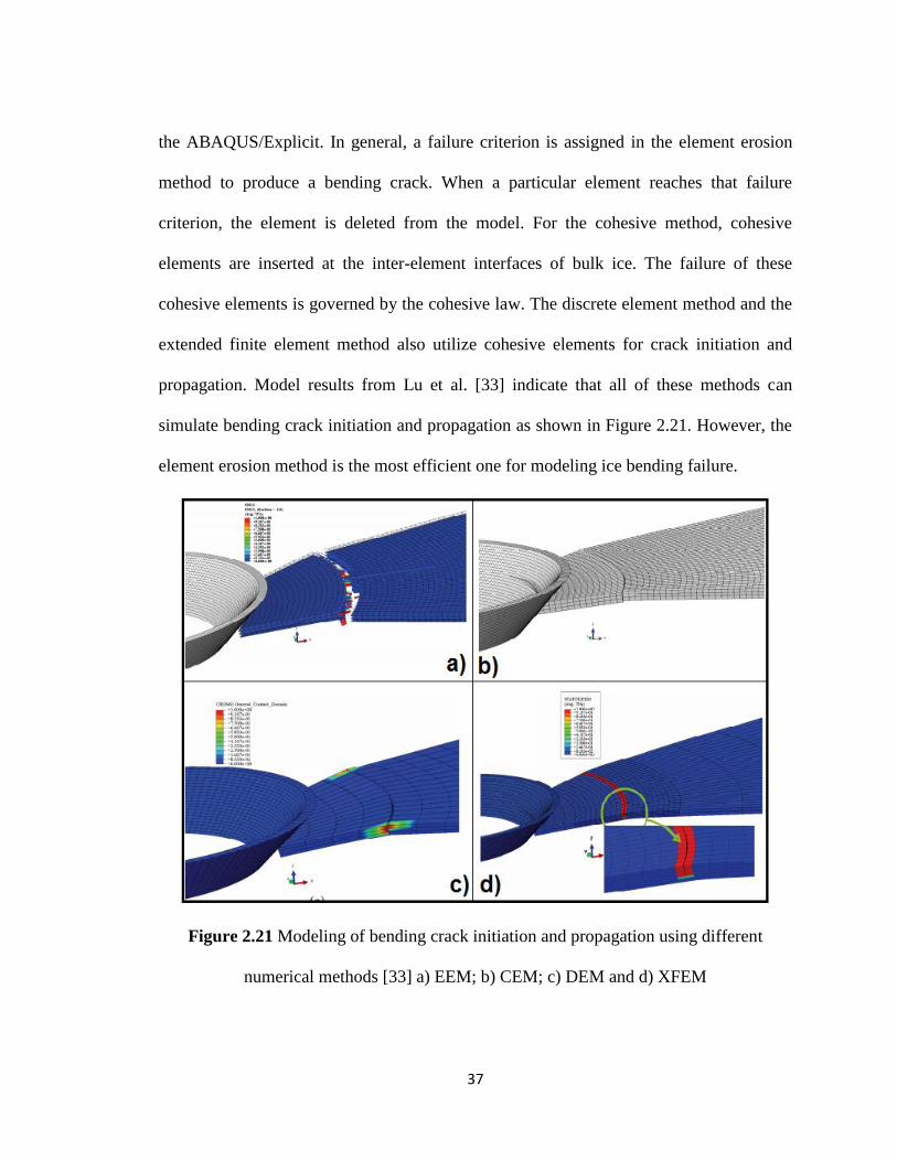
37

the ABAQUS/Explicit. In general, a failure criterion is assigned in the element erosion

method to produce a bending crack. When a particular element reaches that failure

criterion, the element is deleted from the model. For the cohesive method, cohesive

elements are inserted at the inter-element interfaces of bulk ice. The failure of these

cohesive elements is governed by the cohesive law. The discrete element method and the

extended finite element method also utilize cohesive elements for crack initiation and

propagation. Model results from Lu et al. [33] indicate that all of these methods can

simulate bending crack initiation and propagation as shown in Figure 2.21. However, the

element erosion method is the most efficient one for modeling ice bending failure.

Figure 2.21 Modeling of bending crack initiation and propagation using different

numerical methods [33] a) EEM; b) CEM; c) DEM and d) XFEM

38

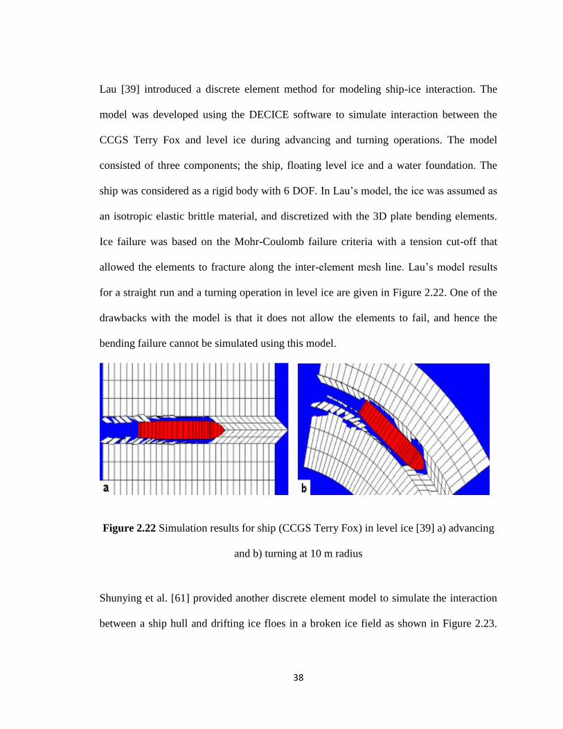
Lau [39] introduced a discrete element method for modeling ship-ice interaction. The

model was developed using the DECICE software to simulate interaction between the

CCGS Terry Fox and level ice during advancing and turning operations. The model

consisted of three components; the ship, floating level ice and a water foundation. The

ship was considered as a rigid body with 6 DOF. In Lau’s model, the ice was assumed as

an isotropic elastic brittle material, and discretized with the 3D plate bending elements.

Ice failure was based on the Mohr-Coulomb failure criteria with a tension cut-off that

allowed the elements to fracture along the inter-element mesh line. Lau’s model results

for a straight run and a turning operation in level ice are given in Figure 2.22. One of the

drawbacks with the model is that it does not allow the elements to fail, and hence the

bending failure cannot be simulated using this model.

Figure 2.22 Simulation results for ship (CCGS Terry Fox) in level ice [39] a) advancing

and b) turning at 10 m radius

Shunying et al. [61] provided another discrete element model to simulate the interaction

between a ship hull and drifting ice floes in a broken ice field as shown in Figure 2.23.

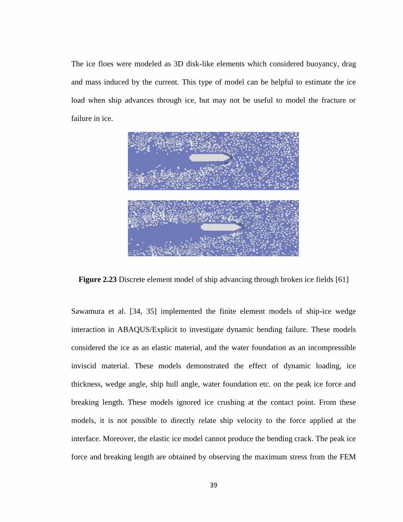
39

The ice floes were modeled as 3D disk-like elements which considered buoyancy, drag

and mass induced by the current. This type of model can be helpful to estimate the ice

load when ship advances through ice, but may not be useful to model the fracture or

failure in ice.

Figure 2.23 Discrete element model of ship advancing through broken ice fields [61]

Sawamura et al. [34, 35] implemented the finite element models of ship-ice wedge

interaction in ABAQUS/Explicit to investigate dynamic bending failure. These models

considered the ice as an elastic material, and the water foundation as an incompressible

inviscid material. These models demonstrated the effect of dynamic loading, ice

thickness, wedge angle, ship hull angle, water foundation etc. on the peak ice force and

breaking length. These models ignored ice crushing at the contact point. From these

models, it is not possible to directly relate ship velocity to the force applied at the

interface. Moreover, the elastic ice model cannot produce the bending crack. The peak ice

force and breaking length are obtained by observing the maximum stress from the FEM

40

results. Figure 2.24 indicates such type of FEM model for a 45o ice wedge rested on the

water foundation along with the boundary conditions and load scenarios.

Figure 2.24 FEM model of ice wedge on water foundation along with edge boundary

condition and loading scenario [35]

The selection of a proper ice material model is important for modeling the ship-

icebreaking process. Ice is strain rate sensitive, and responds differently in tension and

compression. Hence, numerically modeling ice is difficult. However, attempts have been

made in the recent past to model the ice numerically for different applications [54-56, 58,

62]. For an example, Wang et al. [62] developed an ice model for a nonlinear dynamic

FEM model of LNG ship-ice interaction using the commercial software DYTRAN. The

ice was considered as a crushable body and discretized with solid elements. The ship was

discretized with the shell elements and modeled as a deformable body with the elastic-

41

plastic material behavior. The interaction model and the simulated result are presented in

Figure 2.25 which indicates that significant crushing occurs at the ice edge.

Figure 2.25 LNG ship-ice collision model (left) and ice edge crushing (right) [62]

Gagnon and Wang [63], Zong [56] and Kim [64] also developed several crushable foam

models in LS DYNA to represent ice behavior. All of these models were formulated on a

trial and error basis to meet some specific test conditions. Gagnon and Wang’s [63]

crushable foam model was used to simulate a collision between a tanker and a bergy bit.

Kim’s [64] ice model was tuned with the experimentally obtained compressive behavior

of cone-shaped ice specimens. Zong [56] evaluated more than 30 ice crushable foam

models in order to match different pressure-area relationships specified in the Polar Rules

[9]. These models were used to simulate ice crushing behavior. However, suitability of

these models for investigating generalized ice crushing is questionable because of the

insensitivity to strain rate. Moreover, these models apply the same stress-strain

relationship in tension and compression, which make them incapable of modeling

bending behavior.

42

Carney et al. [58] and Pernas-Sanchez et al. [55] proposed plasticity based and strain rate

sensitive ice material models. These models provided different behaviors in tension and

compression which follow the Drucker-Prager yield criterion. These models also

accounted for the strain rate sensitivity in compression, and assumed no sensitivity in

tension. In these models, a pressure cut-off value was assigned for the element failure.

However these models cannot produce a bending crack.

The commercial software LS DYNA [66] has several numerical solvers such as

Lagrangian, Eulerian, Arbitrary Lagrangian Eulerian (ALE), and Smoothed Particles

Hydrodynamic (SPH). Among these solvers, the Lagrangian finite element solver is

computationally efficient and most common for modeling the continuum mechanics

problem. In this solver, the mesh deforms with the material [56]. On the other hand,

material flows through the fixed mesh and allows large deformation in an Eulerian solver.

The ALE solver takes the advantage of both the Lagrangian and the Eulerian solvers and

allows computationally efficient modeling for large deformation problem [55, 56]. For

this reason, the ALE is widely used to model the fluid medium such as water and air in

many fluid-structure interaction problems. Comparisons among three numerical solvers

are illustrated in Figure 2.26.

43

Figure 2.26 Comparisons among Lagrangian, Eulerian and ALE solvers [56]

The SPH is another innovative finite element solver in which the material is represented

as a group of discretized particles [55]. In this mesh free method, particles are linked

together with the material properties [55].

Pernas-Sanchez et al. [55] studied the performance of a plasticity based ice model using

the Lagrangian, Arbitrary Lagrangian Eulerian (ALE) and Smoothed Particles

Hydrodynamic (SPH) solvers. The study indicated that all these numerical solvers can be

used for ice impact analysis. However, comparisons with experimental force time

histories indicated that the Lagrangian solver with the element erosion technique is more

accurate than other two.

The bending strength behavior of ice is crucial for modeling ship-ice interaction. A four

point bending test is commonly used to determine the bending strength and to

44

characterize ice bending behavior. Ehlers and Kujala [54] developed an ice model using a

traditional finite element method to simulate the bending behavior of ice using the

MAT_PLASTICITY_COMPRESSION_TENSION material in LS DYNA. The model

accounted for different responses in compression and tension. Based on bending beam

theory and experimental results, the strain rate effect was assigned to both tension and

compression. A pressure cut off value was defined for the beam failure to obtain a

maximum bending load. The final model results were compared with force-deflection

curves obtained from a four point bending test. The model results were found to be

satisfactory, but did not produce a bending crack as expected to occur in the middle of the

ice beam. Das et al. [65] further studied the ice bending model using a SPH numerical

solver. Identical experimental results and modeling setup were used in this study with the

exception of the failure criteria. The study utilized an equivalent plastic strain value

instead of a pressure cut-off value as the failure criteria. This enabled the model to

generate a bending crack as shown in Figure 2.27.

Figure 2.27 Four point bending model in SPH method indicating bending crack [65]

45

Das’s [65] ice model results indicated that the SPH method with equivalent plastic strain

failure criteria has the potential to simulate the bending failure. However, the SPH

method is known to be computationally expensive and is still in the early stage of

development.

Daiyan and Sand [57] introduced the Cohesive Element Method (CEM) to develop an ice

model in LS DYNA for an ice-structure interaction problem. The model consisted of bulk

ice, cohesive elements, air and a water foundation. The bulk ice was assumed as an

isotropic linear plastic material, and modeled with the material

MAT_PIECEWISE_LINIEAR_PLASTICITY. Two different material properties were

used for cohesive elements in the horizontal and vertical directions to account for the

anisotropic failure behavior. The MAT_COHESIVE_GENERAL material was used for

the cohesive elements which were inserted at the inter-element interfaces of the bulk ice.

These zero thickness cohesive elements enabled the ice model to simulate ice damage

and fracture. In general, the cohesive elements follow a traction-separation curve for

crack initiation and growth. This traction-separation curve was derived based on the ice

fracture mechanics which is directly related to the fracture modes of ice. The air and the

water foundation behavior were simulated using the MAT_NULL to model the fluid-

structure and fluid-ice interactions. The final ice-structure interaction model was applied

to the low velocity interaction problems. The model over predicted the horizontal force

component when compared with the analytical result.

46

2.4 Polar Ship Design Practice

The development of a safe speed methodology for Polar ships is directly related to ship

design practice. A brief discussion of Polar ship design practice follows.

Polar ship design and operation require ice strengthening of the ship structures.

Strengthening ensures structural resistance to ice impact forces. In general, ship

classification societies develop ice strengthening requirements based on ice conditions,

ship structural particulars and ship operating conditions [7, 8, 67]. In addition, each

classification society provides various ice classes in order to guide the ship design and

operation in different ice conditions. Each ice class has its own ice strengthening

requirements [56]. Table 2.1 lists the major classification societies and Rule systems

along with the number of ice classes.

Table 2.1 Major ship classification societies/ rule systems and their ice classes [9, 56]

Ship Classification Societies/Rule Systems Ice Classes

Canadian ASPPR/CAC

9 Classes

Russian MRS/NSR 9 Classes, 4 Icebreaker

Finnish Swedish Ice Class Rules (FSICR) 5 Baltic Classes

American Bureau of Shipping (ABS) 5 Polar Classes , 5 Baltic Classes

Det Norske Veritas (DNV) 3 Icebreaker, 3 Polar, 5 Baltic Classes

Lloyds Register (LR) 5 Polar, 5 Baltic Classes

47

In the recent past, industry pressed for a simple and common system of ice classes for

ship design [9, 56]. In 1993-2006, the IACS and the IMO developed a harmonized set of

ice classes for ships intended to operate in polar waters [9]. The IACS under the guidance

of the IMO developed seven Polar ice classes to replace the member societies’ current

rule sets [7, 9, 67]. The Polar Rules are also known as Unified Requirements for Polar

Ships or the Polar UR. The Polar UR represents the latest industry standards for Polar

ship design and operation [7, 9]. The following sub-sections describe different ice classes,

ice load design methodology and ship structural requirements specified in the Polar Rules.

2.4.1 Polar Ice Classes

The Polar ice rules and Baltic ice rules are the most widely adopted rules for designing

ice class ships. The Finnish-Swedish Maritime Administration (FMA) developed six ice

classes to guide ship operation in winter ice in the Baltic Sea, and the first year ice of

sub-polar regions [6]. The IACS Polar Rules provide seven ice classes to deal with the

multi-year ice along with light first year ice [6]. The descriptions and notations of these

Polar ice classes are given in Table 2.2. In the Polar ice classes, the PC 1 is the upper end

and allows the year-round operation in all polar water without limitations [8, 10]. The PC

7 is the lower end for the summer/autumn operation [8, 9]. Comparison with the Baltic

ice classes indicates that the lowest Polar ice classes PC 6 and PC 7 are equivalent to the

Finnish Swedish Ice Class Rules (FSICR) ice classes IA super and IA, respectively, as

shown in Figure 2.28. The selection of proper ice class is based on the ice conditions,

operational requirements and cost [9].

48

Table 2.2 Description of IACS Polar ice classes [9]

Polar

Class

Ice Description (based on WMO Sea Ice Nomenclature)

PC 1 Year-round operation in all Polar waters

PC 2 Year-round operation in moderate multi-year ice conditions

PC 3 Year-round operation in second-year ice which may include multi-year ice inclusions

PC 4 Year-round operation in thick first-year ice which may include old ice inclusions

PC 5 Year-round operation in medium first-year ice which may include old ice inclusions

PC 6 Summer/autumn operation in medium first-year ice which may include old ice

inclusions

PC 7 Summer/autumn operation in thin first-year ice which may include old ice inclusions

Figure 2.28 Approximate comparisons between Baltic and Polar ice classes [9, 10]

49

Both the Baltic and the Polar Rules require the ice strengthening of ship hull regions.

These strengthening requirements are ice class dependent. In general, the hull regions are

strengthened with the ice belt as indicated in Figures 2.29 and 2.30. Both the rules specify

the ice strengthening requirements for each hull region and ice class. In the Polar Rules,

the entire exterior hull must be strengthened as ice may interact with any part of the hull.

Figure 2.29 Ice strengthening requirements in Baltic ice rules [11]

Figure 2.30 Ice strengthening requirements in Polar ice rules [11]

50

2.4.2 Polar Design Ice Load Scenario

In the Polar Rules, the ice load parameters are rationally linked with design scenarios of

ship-ice interaction [8, 9]. The design scenario considers a glancing collision on the

shoulders of the bow with an ice edge. During this glancing collision, the impact force is

limited by the ice edge crushing or flexural failure [9]. Hence, two ice failure load models

for the ice crushing and ice flexure are required to estimate the design ice load parameters.

The Polar Rules design scenario indicating ice edge crushing and ice flexure is shown in

Figure 2.31.

Figure 2.31 Polar Rules design scenario indicating ice edge crushing and ice flexure [8]

In the ice crushing failure model, the impact force is determined by equating the effective

kinetic energy and energy required to crush the ice [7, 8, 12]. The model incorporates

Popov [74] collision mechanics to simplify the six-degree of freedom (DOF) collision

scenario to a single DOF collision scenario [7, 9]. In addition, the collision model

includes a wedge shape ice edge and a pressure-area relationship. The pressure-area

51

relationship is used to define the ice crushing pressure. The pressure-area relationship

adopted in the Polar Rules can be expressed as [7, 56]:

𝑃 = 𝑃𝑜𝐴𝑛𝑒𝑥

(2.5)

The pressure-area relationship in Eq. (2.5) requires the values of nominal strength (Po)

and exponent (ex) for different ice classes. Table 2.3 lists the values of Po and ex for

different ice classes. The nominal contact area (An) is calculated based on the indentation

geometry. Further discussion on the Popov model, pressure-area relationship and ice

crushing limit load model are given in Chapter 3.

Table 2.3 Parameters for pressure-area relationship in Polar Rules [56]

Polar Class Po , MPa ex

PC 1 6

-0.1

PC 2 4.2

PC 3 3.2

PC 4 2.45

PC 5 2.0

PC 6 1.4

PC 7 1.25

The IACS Polar Rules provide a flexural failure model considering a 1500 ice wedge. The

model does not allow the ice crushing force to exceed the ice flexural force [8]. The

IACS proposed flexural limit load model can be expressed as [7, 12]:

𝐹𝑓𝑙𝑒𝑥_𝑃𝑜𝑙𝑎𝑟 =1.2𝜎𝑓ℎ𝑖𝑐𝑒

2

sin 𝛽′

(2.6)

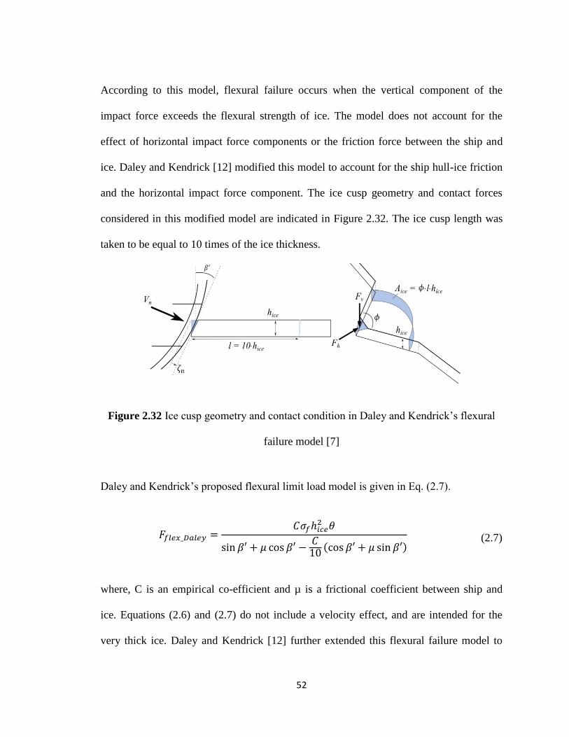
52

According to this model, flexural failure occurs when the vertical component of the

impact force exceeds the flexural strength of ice. The model does not account for the

effect of horizontal impact force components or the friction force between the ship and

ice. Daley and Kendrick [12] modified this model to account for the ship hull-ice friction

and the horizontal impact force component. The ice cusp geometry and contact forces

considered in this modified model are indicated in Figure 2.32. The ice cusp length was

taken to be equal to 10 times of the ice thickness.

Figure 2.32 Ice cusp geometry and contact condition in Daley and Kendrick’s flexural

failure model [7]

Daley and Kendrick’s proposed flexural limit load model is given in Eq. (2.7).

𝐹𝑓𝑙𝑒𝑥_𝐷𝑎𝑙𝑒𝑦 =𝐶𝜎𝑓ℎ𝑖𝑐𝑒

2 𝜃

sin 𝛽′ + 𝜇 cos 𝛽′ −𝐶10(cos 𝛽′ + 𝜇 sin 𝛽′)

(2.7)

where, C is an empirical co-efficient and µ is a frictional coefficient between ship and

ice. Equations (2.6) and (2.7) do not include a velocity effect, and are intended for the

very thick ice. Daley and Kendrick [12] further extended this flexural failure model to

53

thinner ice and higher speed interactions. A Froude scaling method was introduced to

consider the dynamic effect in the flexural failure model [7, 12]. The method scaled the

flexural force with the ratio of dynamic Froude number (FN) and static Froude number

(FNs) as shown in Eqs. (2.8) and (2.9).

𝐹𝑓𝑙𝑒𝑥_𝐷𝑎𝑙𝑒𝑦_𝑑𝑦𝑛𝑎𝑚𝑖𝑐 = 𝐹𝑓𝑙𝑒𝑥_𝐷𝑎𝑙𝑒𝑦 (𝐹𝑁

𝐹𝑁𝑠)𝑛

(2.8)

𝐹𝑁 =𝑉𝑛

√𝑔ℎ𝑖𝑐𝑒

(2.9)

The power (n) and the static Froude number in Eq. (2.8) were chosen as 0.33 and 0.1,

respectively [7]. The model can provide a safe speed calculation. However, the model

needs further improvement.

The minimum impact force from the ice crushing model and the ice flexural model

provides the bow impact load. The bow impact load (Fi) is limited to a rule specified

force value (Fl). The Polar Rules based bow impact load formula can be expressed as [8,

11]:

𝐹𝑖 = 𝑚𝑖𝑛

{

𝐹𝑐 = 𝑓𝑎𝐶𝐹𝑐𝐷

0.64

𝐹𝑓 =1.2𝜎𝑓ℎ

2

𝑠𝑖𝑛 𝛽′

𝐹𝑙 = 0.6𝐶𝐹𝑐𝐷0.64

}

(2.10)

The shape coefficient (fa) in Eq. (2.10) is defined as:

𝑓𝑎 = (0.097 − 0.68 (𝑥

𝐿− 0.15)

2

)𝛼

√𝛽′

(2.11)

54

Equation (2.10) indicates that the bow impact load is a function of ice flexural strength

(σf), ice thickness (h), crushing class factor (CFc), ship displacement (D), impact location

(x) with respect to ship length (L) and different hull angles such as water line angles (α)

and normal ship frame angles (β'). The hull angles at impact locations can be calculated

using Figure 2.33.

Figure 2.33 Hull angle definition in Polar Rules [11]

In the Polar Rules, the bow impact load is calculated at four different bow locations. The

impact load with the maximum magnitude is applied in the form of load patch to evaluate

the structural strength [7-9, 11]. This load patch is acted over a triangular contact surface

and cannot be applied to the ship structure directly [17]. Therefore, the triangular load

patch is idealized to a rectangular load patch using specified formulas. The Polar Rules

based load patch idealization and different load patch parameter calculation procedures

are given in Chapter 6.

55

The hull area factors (AF) are introduced in the Polar Rules to reflect the relative

magnitude of impact load in different hull regions [11]. The AFs for different Polar

classes at various hull regions are given in Table 2.4.

Table 2.4 Hull area factors in Polar Rules [8-11]

Rahman [8] mentioned that measured ice loads can be quite peaky within a rectangular

load patch. The effects of these peak loads are accounted with a peak pressure factor

(PPF). The PPF values for different structural members are given in Table 2.5. The peak

pressure factor magnifies the total patch load, and represents a pressure concentration on

the localized structural members as shown in Figure 2.34.

Table 2.5 Peak pressure factor (PPF) in the Polar Rules [8-11]

56

Figure 2.34 Peak pressure factor on structural member [8, 9]

2.4.3 Structural Limit State Analysis

Structural limit state analysis is important for the Polar ship design as limit states define

the load bearing capacity of the structural members. The limit states determine whether a

structural member will fail or not under the action of a particular design load patch. In

general, the design load patch is applied to a structural member in the horizontal

orientation as shown in Figure 2.35.

Figure 2.35 Application of design load patch to structural member [8]

57

Plates and frames are the primary structural members of Polar ships. The limit states of

the plates and frames are determined based on plastic collapse mechanisms [7-9]. The

IACS Polar Rules contain several analytical expressions for plastic capacity and limit

state conditions for plates and frames [12]. These analytical expressions are derived

based on the energy methods and validated with non-linear finite element analysis [68,

69].

The plastic collapse mechanism in Figure 2.36 is considered by Daley et al. [68] to

determine the plate limit state equations. The figure indicates the possible hinge locations

with different ratio of load height (b) to frame spacing (s) and frame span (l).

Figure 2.36 Plastic collapse mechanisms for plate limit state conditions [9]

For framing, three primary limit state conditions are considered in the Polar Rules. The

collapse mechanisms corresponding to these limit state conditions are shown in Figures

2.37a to 2.37c. Further discussion on the plate and frame design and their limit state

equations is carried out in Chapter 6.

58

Figure 2.37a 1st limit state - 3 hinge formation in plastic frame [68]

Figure 2.37b 2nd limit state - shear panel formation in plastic frame [68]

Figure 2.37c 3rd limit state - end shear in plastic frame [68]

2.5 Current Status of Safe Speed Methodology

Safe speed operation is of current interest to the IMO, classification societies and ship

industries. The concept of Safe Speed is intended to provide operational guidance to

Polar ships in different ice conditions [7, 12]. The concept is not new, yet few studies of

59

the idea are found in the literature. Dolney et al. [7] mentioned that the ice passport or ice

certificate concept was first introduced in the mid 1970s by Russian scientists to ensure

safety of the hull during ice operation, by regulating the ship speeds.

The design ice load model and structural limit state conditions are the primary elements

of the ice passport and safe speed methodology. Several approaches are followed in the

early forms of the Russian ice passport, and in the more recent safe speed methodology,

to obtain the design ice load parameters and structural limit state conditions. The Russian

ice passport considers Kurdyumov and Kheisin’s velocity dependent hydrodynamic

model for the local contact pressure which is combined with Popov collision mechanics

[7]. The structural limit state conditions are obtained from yield and ultimate failure

criteria. This provides two critical curves: a safe speed curve corresponding to yield

criteria and a dangerous speed curve corresponding to ultimate failure criteria. A third

curve of attainable speed in ice is also specified in the Russian passport concept which is

established from the propeller thrust and ice resistance [3, 7]. The Russian ice passport

concept is illustrated in Figure 2.38. Based on this concept Likhomanov et al. [3]

developed an ice passport for the Canadian Coast Guard icebreaker “Pierre Radisson” in

1997. Recently, CNIIMF [70] established an ice certificate identical to the Russian ice

passport for an Arctic Shuttle Tanker (LU 6). CNIIMF’s ice certificate contains a

different curve named as admissible speed curve which is obtained from the minimum of

safe speed and attainable speed curves. CNIIMF’s ice certificate diagram is shown in

Figure 2.39.

60

Figure 2.38 Concept of Russian ice passport [3]

Figure 2.39 CNIIMF ice certificate for Arctic Shuttle Tanker [70]

The recent approach in safe speed methodology utilizes the Polar Rules structural limit

state equations and design ice load model [7]. The plasticity based limit state analysis

avoids over design of shell plating and framing [68, 69].

It is mentioned earlier that the Polar Rules based design ice load model requires an ice

crushing model and an ice flexure failure model. Most of the recent approaches use these

61

two failure models to estimate the design ice load parameters for the safe speed

methodology. The major limitation of these approaches is the flexural failure model

which does not account for the velocity effects. Hence, these approaches are not suitable

for thinner ice or higher ship speed applications.

Daley and Kendrick [12] extended the Polar flexural failure model to account for the

velocity effect. This extended model further utilized to develop the safe speed

methodology for different Polar class ships. The authors developed an excel spreadsheet

named as SAFE.speed.check to allow a simple calculation of safe speed in different ice

conditions. The SAFE.speed.check spreadsheet provides a tool for the safe speed

guidance of Polar class ships. Dolney et al. [7] also utilized the extended model to

develop a safe speed methodology which was illustrated with a PC 5 Ice class ship.

2.6 Literature Summary and Problem Statement

The literature review indicates a requirement to incorporate the velocity dependent ice

flexural failure model into a more comprehensive safe speed methodology. At present

there is no universally accepted dynamic flexural failure model found in the literature.

However, the literature provides information which can be used as the theoretical basis

and technical background for developing a velocity dependent flexural failure model

leading to an improved safe speed methodology. The key information from this literature

is extracted and summarized below to explain the motivation and methodology of the

present work.

62

Increasing shipping activities increase the possibility of accidental events in the

Arctic. Ice class ship design does not always ensure the protection of the Arctic

ship from these accidental events due to the ice actions. The concept of safe ship

speed operation extends the responsibility for safety from the design to the

operation. Therefore, the present work is focused on the development of safe

speed methodology for the Polar ships.

A velocity dependent flexural failure model is an important ingredient of a safe

speed methodology. Current practice in the IACS Polar Rules and most of the

existing models do not consider the velocity effect. Therefore, it is necessary to

develop a velocity dependent flexural failure model.

Development of velocity dependent flexural failure model requires a clear

understanding of the ship-ice interaction process. In general, a ship-ice interaction

process is idealized based on the observation of model scale and full scale tests.

An idealized ship-ice interaction process consists of breaking phase, rotating

phase and sliding phase. Investigation of the entire interaction process,

considering all the phases is important for understanding the global ice force and

the ice resistance. The local peak force is responsible for ship structural damage.

Analysis of the breaking phase of a ship-ice interaction process is sufficient to

extract this local peak force. Hence, the present study considers only the breaking

phase of ship-ice interaction.

63

There is no universally accepted description of the icebreaking pattern. However,

different idealized icebreaking patterns by Kashteljan [29], Enkvist [30], Kortas

[31] and Riska [20] indicate the formation of ice wedges or ice cusps. Many

researchers suggested modeling simple ice wedge breaking instead of the full ice

sheet, especially for the local contact force. The present study also considers the

modeling of ship ice wedge breaking process.

Existing models using the analytical and semi-empirical approaches (Kashteljan

et al. [29], Kheisin [46], Lindqvist [36], Liu [21, 49], Lubbad and Loset [18],

Sawamura et al. [5, 53], Su et al. [14], Zhou et al. [52], Tan et al. [24, 27, 28],

Aksnes [18] etc.) focus mainly on the prediction of the global ice force and ice

resistance for continuous icebreaking and maneuvering operations. Most of these

models are simplified and ignore one or more influencing parameters.

Nevertheless, these models are helpful to understand the individual mechanism

involved in the ship-ice interaction.

Advanced numerical techniques can be employed to develop new ice material

models and ship icebreaking models. These models are valuable in investigating

the dynamic bending behavior. Numerical methods such as FEM, CEM, DEM

and XFEM [33, 35, 39, 54-59, 61-64], and different numerical solvers such as

Lagrangian, ALE and SPH are employed for these modeling purposes. Many of

these methods and solvers have the capability to generate the bending crack

initiation and propagation. However, the finite element method with the element

64

erosion technique and the Lagrangian solver is indicated to be the most efficient

method and hence is adopted in this study.

Model validation is crucial for the acceptance of a developed model. Most of the

ship-ice interaction models, which are intended to predict global ice forces and

resistance forces, are validated against model scale and full scale tests. However,

model scale and full scale tests are of limited value in characterizing the local

contact mechanism. Many researchers (Daiyan and Sand [57], Sawamura et al.

[34, 35] etc.) use analytical or semi-empirical approachs to validate their local

contact force models. The present study validates the developed flexural failure

model by comparing with existing analytical and semi-empirical models.

Design ice load patch and structural limit state equations are the final element

needed to develop the safe speed methodology. The IACS Polar Rules have well

established procedures and guidelines to idealize the load patch parameters from

calculated bow impact loads, and to determine the structural limit state equations

from the plastic collapse mechanism. These procedures and guidelines are

adopted in the present study.

65

Chapter 3

Material Models for Ice and Water (in LS DYNA)

3.1 Introduction

Material models are important to characterize the ice failure processes and to understand

the water foundation effect in the icebreaking process. In general, the icebreaking process

involves ice crushing and flexural failures which are influenced by the water foundation

under ice. Three numerical tests are conducted in the commercial software package LS

DYNA to develop material models of ice crushing failure, ice flexural failure and water

foundation. This chapter provides a brief discussion of the icebreaking process explaining

the ice failure processes and the water foundation effect, followed by a detailed procedure

and methodology to develop these material models. A short discussion of the LS DYNA

modeling approach is also presented in this chapter.

66

3.2 Ice Failure in Ship Icebreaking

Previous studies on ship-ice interaction process have shown that the icebreaking process

is responsible for the local peak force. Therefore, only the icebreaking process is

considered in this study. In general, an icebreaking process consists of edge crushing,

flexural bending, and water foundation effect. A schematic diagram of the ship

icebreaking process is shown in Figure 3.1.

Figure 3.1 Fundamental ship icebreaking process

The ship icebreaking process is complex. The dynamic nature from ice inertia and water

foundation makes the process even more complicated. When a ship interacts with ice at

different velocities, the ice is subjected to dynamic loading. The ice behavior under this

dynamic loading condition is drastically different from its behavior to a static loading

condition. Therefore, it is very important to clearly understand the ice behavior and

physics involved in ice failure when the ice is subjected to different dynamic loading

conditions. This may facilitate the development of a simulation tool to better characterize

the ship icebreaking process. The following sub-sections describe the ice crushing failure,

flexural failure mechanisms and water foundation effect on the breaking process.

67

3.2.1 Ice Crushing Failure

When a ship interacts with the level ice, crushing takes place at the ice edge before

flexural failure initiates and propagates. The crushing area at the contact interface

increases as the ship advances. The normal impact force (Fn) also increases with the

contact area until the flexural failure occurs. This normal impact force (Fn) can be

determined from the nominal contact area (An) and average contact pressure using Eq.

(3.1).

𝑃𝑎𝑣𝑔 =𝐹𝑛𝐴𝑛

(3.1)

The LS DYNA provides direct measurement of normal impact force. However, the

contact area cannot be found easily. Daley [50] derived a number of useful contact area

equations for different indentation geometry cases. These contact area equations are

applicable to both ship-ice interaction and ice-structure interaction problems. Figure 3.2

is the indentation geometry of a wedge-shaped ice edge which is used to calculate the

contact area. Daley’s calculated contact area for an ice wedge is a function of hull

geometry, hull position and ice wedge geometry. The contact area of an ice wedge is

related to the ice wedge angle (θ), ship normal frame angle (𝛽′) and normal indentation

(ζn). The equation for the contact area of an ice wedge edge is:

𝐴𝑛 =𝜁𝑛2. 𝑡𝑎𝑛(𝜃 2⁄ )

𝑠𝑖𝑛 𝛽′ . 𝑐𝑜𝑠2(𝛽′)

(3.2)

68

Figure 3.2 Indentation geometry of wedge-shaped ice for contact area calculation [50]

Direct measurement of normal impact force and the calculated contact area from Eq.

(3.2) can be used to obtain the average contact pressure at the wedge-shaped ice edge

from Eq. (3.1). In many studies this average contact pressure is assumed as constant over

the whole contact area to determine the normal impact force [5, 21, 24, 53]. In reality,

this contact pressure is not constant and changes with the contact area [4, 28]. It is

mentioned earlier that the IACS Polar Rules adopted the pressure-area relationship to

account for pressure variation at the contact interface. In the pressure-area relationship,

the average contact pressure follows a decreasing pattern with the contact area as shown

in Eq. (3.3).

𝑃𝑎𝑣𝑔 = 𝑃𝑜𝐴𝑛𝑒𝑥

(3.3)

In Eq. (3.3), the nominal ice strength (Po) is the pressure to crush 1 m2 ice. This pressure-

area relationship is also incorporated into the present study. To establish a pressure-area

69

relationship at the contact interface, the average pressure from the developed numerical

model is calculated using Eq. (3.1) and tuned with a Polar class 1 (PC 1) pressure-area

relationship given in Eq. (3.3). For PC 1 ships, the Po is 6 MPa and the exponent (ex) is -

0.1 [56]. The Po value changes for other Polar class ships as shown previously in Table

2.3.

3.2.2 Ice Flexural Failure

A ship or sloping structure breaks the level ice in flexure. In flexure, when the vertical

component of impact force exceeds the flexural limit, a flexural crack initiates and

propagates. In general, the ice has much lower flexural strength (approximately 10 times

less) than the crushing strength [54]. This can result in lower ice loads in flexural failure

than for cases where the ice fails in crushing especially in thinner ice. Several analytical

and semi-empirical models exist for the ice flexural failure. Most of these models express

the failure load (Ff) as a function of ice flexural strength (σf), wedge angle (θ) and ice

thickness (h). Kashteljan’s bending failure model, given in Eq. (2.2), is widely used to

predict the bending failure load. This semi-empirical model is based on the bearing

capacity of a floating ice wedge. The model is rewritten here as this will be used for

different comparative analysis in the present study:

𝐹𝑓 = 𝐶𝑓 (𝜃

𝜋)2

𝜎𝑓ℎ2

(3.4)

70

The empirical coefficient (Cf) in Eq. (3.4) is approximately 1 for Kashteljan’s model [14].

Daley and Kendrick [12] proposed a model similar to the Polar Rules flexural failure

model as shown below:

𝐹𝑓 = 𝐶𝑓𝜎𝑓ℎ2𝜃 (3.5)

Daley and Kendrick [12] mentioned that the value of the coefficient Cf is 0.46 in the

Polar Rules for a 150o wedge. Further, the Cf value is corrected to 0.39 by Daley and

Kendrick. Equations (3.4) and (3.5) are applicable to the static or quasi-static conditions.

The ice flexural failure under a dynamic loading condition is significantly different from

the static or quasi-static loading conditions. The ship with higher velocity is expected to

experience a higher impact force from the ice. Unfortunately, there is no suitable dynamic

flexural failure model available to explore this ship velocity effect. Therefore, a

methodology is presented in Chapter 4 to estimate the dynamic flexural failure load based

on different existing static load models and dynamic factor models.

3.2.3 Water Foundation Effect

Water under a floating ice sheet acts as an ideal elastic foundation for the ice. The

foundation creates a hydrostatic pressure on the ice and influences the breaking process.

In the presence of a foundation, the hull requires higher force to break the ice. Moreover,

higher ship velocity modifies the hydrodynamic pressure of the water foundation and

results in a significant increase in the ice load. The water foundation can be considered as

a soft linear elastic material having a low modulus of elasticity (Ew) and standard water

71

density (ρw). The hydrostatic pressure (Phs) can be expressed as a function of vertical

deflection of the ice wedge (ϑ) in the following equation:

𝑃ℎ𝑠 = 𝜌𝑤𝑔𝜗 (3.6)

3.3 Material Models for Ice and water

For a good ship icebreaking model, the selection of proper material models and input

parameters are important. Three individual numerical tests are conducted to select the

material models and parameters for the ice crushing behavior, ice flexural behavior and

water foundation effect. The models and parameters are used in the final ship icebreaking

model which will be described in Chapter 4. For the ice crushing material model, an ice

crushing test is performed. A four point bending test provides the material model of ice

flexure, and a simple foundation test is conducted to select the material properties of

water foundation.

There are several commercial finite element software packages available. In this analysis,

the LS DYNA is used to develop the material models for ice and water. The LS DYNA is

widely used as a numerical tool for analyzing the impact and non-linear dynamic

problems. It has a large collection of material models, and capable of modeling different

material failure modes, crack initiation-propagation, crushing etc. A general guideline of

the finite element methodology and modeling approach of LS DYNA is shown in Figure

3.3. The LS DYNA methodology and modeling approach for material models and

properties of ice crushing, ice flexure and water foundation are described in Sub-sections

72

3.3.1 to 3.3.3. The LS DYNA Keyword files of these material models are presented in

Appendix A.

Figure 3.3 Methodology and modeling approach in LS DYNA

STEP 4: ANALYZE THE OUTPUTS

# Force # Stress

# Strain # Others

Post

-Pro

ces

sin

g

No

Application

STEP 1: BUILD THE MODEL

# Geometric Model # Meshing

# Material Properties # Section Properties

STEP 2: DEFINE LOAD & BOUNDARY CONDITIONS

# Applied Loads # Constrains

# Contacts # Others

STEP 3: DEFINE SOLUTION & OUTPUT PARAMETERS

# Simulation Time # Time Step

# Output Parameters

Pre-

Pro

cess

ing

Yes

Refine

Expected Results

73

3.3.1 Material Model for Ice Crushing

An ice crushing test is performed to develop a material model for the ice crushing

behavior. In this test, an inclined indenter impacts and crushes the edge of a short ice

wedge. The geometric model of the crushing test is shown in Figure 3.4. The indenter is

assumed as a rigid steel material and discretized with the shell elements. A simple elastic-

perfectly plastic material model *MAT_PLASTIC_KINEMATIC is used for the ice

wedge. The input parameters of the model are estimated from the physical and

mechanical properties of ice. The compressive strength (σc) and Young’s modulus (E) of

ice are tuned to establish a similar pressure-area relationship suggested in the Polar Rules

for PC 1. The details of the indenter and ice wedge are shown in Table 3.1 and 3.2,

respectively.

Figure 3.4 Geometric model of ice crushing test indicating indenter and short ice wedge

74

Table 3.1 Details of indenter in ice crushing test

Dimensions 2x4x0.37 m; 450 inclined

Element type SHELL

Material card *MAT_RIGID

Density, ρ 7850 kg/m3

Young modulus, E 200 GPa

Poisson’s ratio, υ 0.3

Table 3.2 Details of ice wedge in ice crushing test

Dimensions 300 wedge; 2 m thick; 3 m length

Element type SOLID

Material card *MAT_PLASTIC_KINEMATIC

Comp. strength, σc 4.5 MPa




In the test, the rigid indenter is moved horizontally towards the ice wedge with a velocity

of 0.5 ms-1. The bottom surface of the ice wedge is fixed in all DOFs. As the indenter

advances, both the interface force and contact area are increased. Figure 3.5 indicates the

change in Von-Mises stress distribution and crushing area at two different times.

75

Figure 3.5 Von-Mises stress distribution and change in crushing area

The impact force time history is observed and recorded using the LS-PrePost software

(also from lstc.com). For a 300 ice wedge and 450 indenter, the contact area in Eq. (3.2)

can be written in terms of indenter velocity (V) and time interval (t):

𝐴𝑛 = 0.295 (𝑉𝑡)2 (3.7)

The normal impact force and contact area time histories from the crushing test are

presented in Figure 3.6. The figure indicates that both the impact force and contact area

increase with time.

Figure 3.6 Normal impact force and contact area time histories in ice crushing test

0

1000000

2000000

3000000

4000000

5000000

6000000

0 0.5 1 1.5 2 2.5 3

Normal Impact Force [N]

Contact Area [mm^2]

Time, Sec

76

A model pressure-area curve is established using the contact area and the normal impact

force time histories given in Figure 3.6. This model pressure-area curve and the PC 1

pressure-area curve from Eq. (3.3) are plotted in Figure 3.7. The model results are in

reasonable agreement with the PC 1 pressure-area relationship. Both the curves indicate

the decreasing trends of average pressure with the contact area although there is some

fluctuation about the mean trend in the model. The triangular shaped fluctuations in the

model pressure–area curve are due to coarse element size in the crushing model. This

coarseness of the element may influence the crushing failure pattern slightly but it will

not affect the magnitude of bending failure load in the final numerical ship icebreaking

model.

Figure 3.7 Comparison between model and PC 1 pressure-area curves

5

9

13

17

0.001 0.01 0.1 1

Model Pressure Area Curve

PC-I Pressure Area Curve

Pre

ssu

re,

MP

a

Area, m2

77

3.3.2 Material Model for Ice Flexure

Four point bending tests and in-situ cantilever beam tests are the most widely used and

acceptable method to characterize the ice flexural failure behavior. Both the tests are

capable of generating flexural cracks. The cantilever beam test with the element erosion

modeling technique may exhibit some local crushing at the loading point. Therefore, the

present study performs a numerical four point bending test in order to achieve pure ice

flexure behavior. In this type of four point bending test, the whole beam between the two

load points (loading supports) is subjected to be constant bending moment and is not

affected by the direct compression below the load.

A similar geometric configuration of four point bending test used in Ehlers and Kujala

[54] is considered in the present study. Ehlers and Kujala’s four point bending test model

and measurements do not provide all the required material parameters. Therefore, the

present study utilizes different material input parameters and compares the test results

with theoretical results.

From a four point bending test, it is possible to determine the maximum bending load and

bending crack location. The theoretical failure load in bending (Fb) can be calculated

from the following equation:

𝐹𝑏 =𝜎𝑓𝑊𝐻

2

3𝐷

(3.8)

where, W, H and D are the beam width, height and distance between upper and lower

supports, respectively. In a four point bending test, the maximum bending moment occurs

78

at the mid-section of the beam. Hence, the bending crack occurs in the mid-section. The

material model of ice flexure is developed by comparing the model results with the

theoretical bending loads calculated from Eq. (3.8), and by observing the crack locations.

In the test, the upper supports and lower supports are placed at a distance of 2 m and 0.5

m, respectively, from the center of the ice beam. The element type and material

properties listed in Table 3.1 are used for all the supports. The geometric model of four

point bending model is given in Figure 3.8.

Figure 3.8 Geometric model of four point bending test

For the ice beam model, the input parameters are selected based on the physical and

mechanical properties of sea ice [33, 54, 57, 63]. An isotropic elasto-plastic model,

*MAT_PLASTICITY_COMPRESSION_TENSION is used to represent the ice flexural

failure. The model requires several material parameters and curves. The main reason for

selecting this material model is its ability to model different responses in compression

and tension. Moreover, it can also account for the strain rate sensitivity. The details of

geometric dimensions and material properties are given in Table 3.3.

79

Table 3.3 Details of ice beam in four point bending test

Dimensions 4.32x0.365x0.392 m; distance between upper

and lower supports (D), 1.5 m

Element type SOLID

Material card *MAT_PLASTICITY_COMPRESSION_TENSION




Initial comp. strength, σco 5.8 MPa

Initial tensile strength, σto 0.1σc

o

Plastic hardening modulus, Ep 6 MPa

Effective plastic failure strain, ϵf 7.0e-4

Compressive mean stress, σmc 𝜎𝑐𝑜

3⁄

Tensile mean stress, σmt 𝜎𝑡𝑜

3⁄

Three different material curves are used in this analysis. Two different yield stress vs

effective plastic strain curves are used, one for tension and one for compression. The

third curve is a strain rate vs scaled compressive yield stress factor (CYSF) curve which

is used to account for the strain rate effect on compressive strength. It is assumed that the

flexural strength is independent of strain rate. Both the curves of yield stress (σy) vs

effective plastic strain (ϵp) in tension and compression are developed from the following

equation:

𝜎𝑦 = 𝜎𝑦𝑜 + 𝐸𝑝𝜖𝑝 (3.9)

80

where, the same plastic hardening modulus (Ep) is assumed for both the compression and

tension. The initial compressive yield strength (σco) is calculated at 10-3 s-1 strain rate (ϵ̇)

from the following equation given by Pernas-Sanchez et al. [9]:

𝜎𝑐𝑜 = 10.976𝜀̇0.093783 (3.10)

The equation (3.10) indicates the relationship between the strain rate and compressive

strength. This relationship was established based on several experimental results (Figure

3.9).

The initial yield strength in tension (𝜎𝑡𝑜 ) is assumed 10 times less than the initial

compressive strength [54]. To formulate the strain rate vs compressive yield stress scale

factor (CYSF) curve, the initial compressive strengths at different strain rates are

determined from Eq. (3.10). These compressive strengths are further normalized with the

compressive strength (5.8 MPa) at 10-3 s-1. The Strain rates and the corresponding

compressive yield stress scale factors (CYSF) are shown in Table 3.4.

Figure 3.9 Relationship between compressive strength and strain rate [9]

81

Table 3.4 Strain rates and compressive yield stress scale factors

�̇�, s-1 CYSF �̇�, s-1 CYSF

10e-9 0.27 10e-2 1.22

10e-8 0.336 10e-1 1.52

10e-7 0.417 1.0 1.89

10e-6 0.52 10.0 2.348

10e-5 0.643 100.0 2.91

10e-4 0.8 1000.0 3.62

10e-3 1.0

An equivalent plastic strain failure criterion is used in this analysis. When the equivalent

plastic strain of an element reaches the defined critical value (ϵf), the element is deleted.

The ϵf value is adjusted to get the proper bending response.

To achieve bending failure at quasi-static condition, the lower supports are given an

upward velocity of 0.001 ms-1. The upper supports are constrained in all DOFs, while the

lower supports are allowed only to move in the vertical direction. The reaction force,

between the ice beam and supports, increases with time until it reaches the flexural limit

of ice. The effective plastic failure strain value is tuned until the bending crack is

observed at the mid section of the beam and the model bending load is close to the

theoretical bending load. Figures 3.10 and 3.11 indicate the bending crack formation and

force-time history obtained from the four point bending test. Figure 3.11 indicates that

the ice beam fails at 7.74 kN which is close to the analytical failure load (7.78 kN)

calculated from Eq. (3.8).

82

Figure 3.10 Bending failure of ice beam in four point bending test

Figure 3.11 Force-time history in four point bending test

It should be noted that the material properties of this model are different from the Ehlers

and Kujala’s [54] four point bending test models and measurements. Therefore, the force

time history obtained from this model cannot be compared with the Ehlers and Kujala’s

four point bending test results.

0

1000

2000

3000

4000

5000

6000

7000

8000

9000

0 0.5 1 1.5 2 2.5 3 3.5 4

Ben

din

gF

orc

e,

N

Time,s

83

3.3.3 Material Model for Water Foundation

Modeling of a fluid medium or water foundation is still a big challenge. The existing

material models of water foundation are complicated and computationally expensive.

Therefore, an alternative and simple methodology is introduced here to develop the

material model of water foundation which provides an equivalent hydrostatic pressure on

the bottom surface of the ice wedge.

Simple foundation tests are conducted to select the material properties of water

foundation. The test is carried out for three different ice thicknesses (h) and four different

wedge angles (θ). The foundation is assumed as a linear elastic material, and modeled

with the material card *MAT_ELASTIC. The dimensions and elastic modulus are

adjusted to match as close as possible to the hydrostatic pressure of water on the lower

ice surface. The details of water foundation are given in Table 3.5.

Table 3.5 Details of water foundation

h, θ Dimensions

LxWxH

Density, ρw Young modulus, Ew

0.5, 300 8.5x4.6x1.7 m

1000 kg/m3

13.63 kPa

1.0, 300 16x9x1.8 m 17.4 kPa

1.5, 300 24.7x15x3 m 29.3 kPa

0.5, 450 8.5x6.8x0.8 m 7.78 kPa

0.5, 600 8.5x8.6x0.8 m 8.0 kPa

1.0, 450 16x13.1x1.8 m 17.0 kPa

1.5, 600 24.7x26.7x3 m 28.4 kPa

0.5, 1500 8.5x15.8x1.7 m 15.32 kPa

84

In these tests, the ice wedge is assumed as a rigid solid body so that the reasonable Young

modulus values of water foundation can be obtained within efficient computational time.

The rigid material properties listed in Table 3.1 are used for the ice wedge. Figure 3.12

indicates the geometric model of water foundation test for a 0.5 m thick and 300 ice

wedge on the elastic foundation.

Figure 3.12 Geometric model of water foundation test for 0.5 m thick and 300 ice wedge

In these tests, the ice wedges are allowed to move vertically downward with a velocity of

0.001 ms-1. The bottom and side faces of the water foundation are fixed in all DOFs. The

contact card CONSTRAINT_NODES_TO_SURFACE is assigned to define the contact

between the ice wedges and water foundations. The interface pressure between the ice

wedges and foundations is measured by a numerical force sensor

(FORCE_TRANSDUCER_CONSTRAINT). The interface pressure distribution for the

0.5 m thick ice wedges with 300 and 600 opening angles are shown in Figure 3.13 and

3.14, respectively. These figures indicate that a higher surface area on the water

85

foundation is required to capture the complete interface pressure distribution of an ice

wedge with a higher opening angle. Therefore, the dimensions of the water foundations

are varied for different ice wedge angles as shown in Table 3.5. The dimension of water

foundation for the higher ice wedge angle (1500 wedge) would be used for other cases.

However, this is not recommended for the lower ice wedge angles because of

computational efficiency.

Figure 3.13 Interface pressure distribution for 0.5 m thick and 300 ice wedge

Figure 3.14 Interface pressure distribution for 0.5 m thick and 600 ice wedge

86

The interface pressure time history is recorded and used to establish a relationship

between the average hydrostatic pressure and vertical deflection of the ice wedge. The

pressure deflection curve in Figure 3.15 provides a slope of 9778.9 Pa/m which is

equivalent to the theoretical value calculated from Eq. (3.6). Similar results are obtained

for other test conditions.

Figure 3.15 Pressure deflection curve for 0.5 m thick and 300 ice wedge

It should be noted that the primary objective of developing simplified material models is

to capture the overall ship icebreaking scenario especially the ice flexural behavior. For

faster and more stable solution, some compromises are done with the overall quality of

the ice crushing model and water foundation model. The element size in the crushing

model is relatively coarse which causes the triangular shaped fluctuations in the pressure-

area curve. The water foundation is modeled as a “soft” solid rather than a fluid which

would require use of ALE or other expensive fluid modeling techniques.

y = 9778.9x

0

20

40

60

80

100

120

0 0.002 0.004 0.006 0.008 0.01

Deflection, m

Pre

ssu

re,

Pa

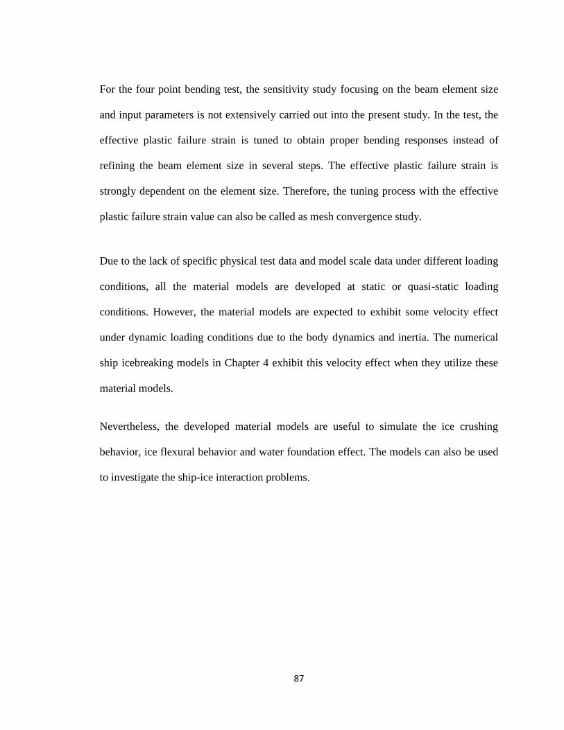
87

For the four point bending test, the sensitivity study focusing on the beam element size

and input parameters is not extensively carried out into the present study. In the test, the

effective plastic failure strain is tuned to obtain proper bending responses instead of

refining the beam element size in several steps. The effective plastic failure strain is

strongly dependent on the element size. Therefore, the tuning process with the effective

plastic failure strain value can also be called as mesh convergence study.

Due to the lack of specific physical test data and model scale data under different loading

conditions, all the material models are developed at static or quasi-static loading

conditions. However, the material models are expected to exhibit some velocity effect

under dynamic loading conditions due to the body dynamics and inertia. The numerical

ship icebreaking models in Chapter 4 exhibit this velocity effect when they utilize these

material models.

Nevertheless, the developed material models are useful to simulate the ice crushing

behavior, ice flexural behavior and water foundation effect. The models can also be used

to investigate the ship-ice interaction problems.

88

Chapter 4

Numerical Model of Ship Icebreaking

4.1 Introduction

This chapter presents numerical models of the ship icebreaking process to explore the

velocity effect on ice flexural failure. These numerical models account for the ice edge

crushing, ice flexural failure and water foundation effect. The material models developed

in Chapter 3 are incorporated into these ship icebreaking models. Two breaking

conditions; an ice wedge breaking condition and a level icebreaking condition are

considered for the head-on collision and shoulder collision scenarios. For the ice wedge

breaking, the effect of ship velocity on the breaking process is investigated for different

ship angles, ice wedge angles and ice thicknesses. The level icebreaking is investigated

with and without existing radial cracks for three different breaking conditions.

In the absence of a standard dynamic ice load model, a simple methodology is presented

to formulate four dynamic ice load models based on existing static load models and

89

dynamic factor models. Two existing analytical/semi-empirical formulas are also

presented to predict the ice wedge breaking length. To validate the numerical models, the

results are compared with the formulated dynamic ice load models and presented

breaking length formulas. The developed numerical models of ship icebreaking as well as

the formulated dynamic ice load models can be useful in estimating the ice load on the

ship or offshore structure.

4.2 Numerical Model of Ship Icebreaking

The numerical models of ship icebreaking consider two collision scenarios. One is the

head-on collision with a flat inclined face of ship, and another is the shoulder collision

with an R-Class ship. For the head-on collision, two breaking conditions are considered;

the ice wedge breaking and level icebreaking. The shoulder collision is only investigated

for the level icebreaking. Both the collision scenarios with all the ship icebreaking

conditions are numerically modeled using the commercial FEM software package LS

DYNA. Sub-sections 4.2.1 and 4.2.2 describe the LS DYNA modeling approach for these

two collision scenarios. Appendix B consists of the LS DYNA keyword files for the ship

icebreaking models.

4.2.1 Head-on Collision with Flat Inclined Face of Ship

For the head-on collision, two icebreaking scenarios are considered; a simple ice wedge

breaking and a level icebreaking. A rigid ship with a flat inclined face is considered to

study this head-on collision. The front inclined face of the ship results in a waterline

90

angle (α) of 900. This simple ship shape allows the investigation of the striking angle

effect on the icebreaking process. In a real ship type, the striking angle is equivalent to

the normal ship frame angle (𝛽′).

4.2.1.1 Simple Ice Wedge Breaking

The numerical model of ship and simple ice wedge consists of three main components; a

rigid ship, a cantilever ice wedge and a water foundation. In the model, a flat inclined

face of the rigid ship impacts the edge of a cantilever ice wedge. The ice wedge rests on

the water foundation. Figure 4.1 shows the geometric model of the rigid ship. The

material properties for the rigid indenter mentioned in Table 3.1 are also used for this

ship.

Figure 4.1 A rigid ship for ship icebreaking model

The ship is discretized with the shell elements, and constrained in all DOFs except the

horizontal direction. Three different normal ship frame angles are considered. The

principal dimensions of the ship are shown in Table 4.1.

91

Table 4.1 Principal dimensions of ship

Parameters Value

Length, L 100 m

Beam, B 20 m

Depth, D 7 m

Normal ship frame angle, 𝛽′ 450, 550, 650

For the ice wedge models, three different ice thicknesses (0.5 m, 1.0 m and 1.5 m) and

three different ice wedge opening angles (300, 450and 600 ) are considered. These ice

wedges have two distinct zones; the ice crushing zone and the ice bending zone as shown

in Figure 4.2. Both zones share common nodes and no duplicate node exists between

these two zones. The length of these wedges is 15h having crushing zone length of 1.85h.

It is assumed that no bending failure occurs within this crushing zone. The ice crushing

material model developed earlier is used for this zone. The remaining portion of the ice

wedges is the bending zone. The material properties mentioned in sub-section 3.3.2 are

used for this zone.

Figure 4.2 Top view of ice wedge indicating ice crushing and bending zones

92

The Element Erosion Method (EEM) is used in this model to obtain ice bending failure.

In this method, when the equivalent plastic strain of an element reaches the defined

critical value (ϵf), the element is deleted. The critical value (ϵf) is highly dependent on the

element size. The ice wedge is meshed such that the same element-length ratio, used in

the four point bending test, is maintained in the analysis.

The dimensions and material properties in Table 3.5 are used for water foundation

modeling. The bottom and side faces of the water foundation are fixed in all DOFs. The

final ship icebreaking model is shown in Figure 4.3.

Figure 4.3 Final model of ship ice wedge breaking process in head-on collision

93

The model requires proper contact definition between the components. The

AUTOMATIC_NODES_TO_SURFACE contact model is used to define the interaction

between the ship and ice crushing zone. The water foundation is constrained to the ice

wedge with the CONSTRAINT_NODES_TO_SURFACE model. It is assumed that no

interaction takes place between the ship and water foundation. The time step factor in the

model is set to 0.6 for stable solution. The final model code is compiled using the LS

DYNA Program Manager, and runs until the ice beam fails in flexure.

4.2.1.2 Level Icebreaking (1500 Ice Wedge)

For the level icebreaking conditions, a similar numerical approach of simple ice wedge

breaking is used. The ice wedge with 1500 opening angle is assumed as equivalent to the

level ice sheet. Three breaking conditions are considered to study the effect of radial

cracks. The first condition is the breaking of single 1500 ice wedge without any radial

crack. The second condition is the breaking of ice wedge with two radial cracks. The ice

wedge with two radial cracks consists of three 500 ice wedges. The third condition is the

breaking of five 300 wedges which contain four radial cracks. The radial cracks separate

the ice wedges with duplicated nodes. These duplicated nodes create area of weakness

between two adjacent wedges which represent the existing radial crack in the level ice.

This analysis is performed for a normal ship frame angle of 650 and ice thickness of 0.5

m. Figure 4.4 is the geometric model of ship level icebreaking for five 300 wedges rested

on the water foundation.

94

Figure 4.4 Ship level icebreaking in head-on collision indicating wedges separated with

duplicated nodes

4.2.2 Shoulder Collision with R-Class Ship

This sub-section demonstrates the modeling of shoulder collision scenario with a real

ship type similar to the IACS Polar design scenario. In this model, the level ice or 1500

ice wedge interacts with the shoulder region of an R-Class ship. The R-Class ship is

constructed from the ship parameters, bodylines and body planes diagram given in

Makinen et al. [71]. Only the front half portion of the ship is considered here. At the

contact point, the waterline angle and normal ship frame angle are 32.50 and 550,

respectively. The level icebreakings with four radial cracks and without a radial crack are

investigated. Figure 4.5 is the collision model for the R- Class ship with the level ice.

95

Figure 4.5 Shoulder collision with R-Class ship

4.3 Model Results and Analysis

The numerical results of icebreaking process for both the collision scenarios are

presented here. The effect of ship velocity on the impact force and ice failure pattern is

investigated for all the icebreaking processes.

4.3.1 Simple Ice Wedge breaking in Head-on Collision

Velocity Effect on Breaking Pattern

The Von Mises stress distribution and failure pattern of the simple ice wedge breaking for

different breaking conditions are shown in Figures 4.6a to 4.6g. These figures indicate

that the crushing is observed at the edge for all the breaking conditions. The

circumferential bending crack initiates and propagates in the bending zone. For a

96

particular ship frame angle, ice thickness and ice wedge; the bending crack location shifts

towards the ice crushing zone at higher ship velocity (Figures 4.6a to 4.6d). These figures

also indicate that the bending crack location and breaking pattern are influenced by the

wedge angle (Figure 4.6a and 4.6e), ice thickness (Figure 4.6c and 4.6f) and normal ship

frame angle (Figure 4.6b and Figure 4.6g).

Figure 4.6a Simple ice wedge breaking pattern (h=0.5 m, β′=650, θ= 300, V=0.1 ms-1)

Figure 4.6b Simple ice wedge breaking pattern (h=0.5 m, β′=650, θ= 300, V=0.5 ms-1)

97

Figure 4.6c Simple ice wedge breaking pattern (h=0.5 m, β′=650, θ= 300, V=1.0 ms-1)

Figure 4.6d Simple ice wedge breaking pattern (h=0.5 m, β′=650, θ= 300, V=5.0 ms-1)

98

Figure 4.6e Simple ice wedge breaking pattern (h=0.5 m, β′=650, θ= 450, V=0.1 ms-1)

Figure 4.6f Simple ice wedge breaking pattern (h=1.5 m, β′=650, θ= 300, V=1.0 ms-1)

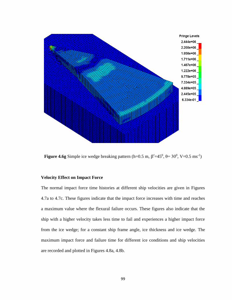
99

Figure 4.6g Simple ice wedge breaking pattern (h=0.5 m, β′=450, θ= 300, V=0.5 ms-1)

Velocity Effect on Impact Force

The normal impact force time histories at different ship velocities are given in Figures

4.7a to 4.7c. These figures indicate that the impact force increases with time and reaches

a maximum value where the flexural failure occurs. These figures also indicate that the

ship with a higher velocity takes less time to fail and experiences a higher impact force

from the ice wedge; for a constant ship frame angle, ice thickness and ice wedge. The

maximum impact force and failure time for different ice conditions and ship velocities

are recorded and plotted in Figures 4.8a, 4.8b.

100

Figure 4.7a Impact force vs time in simple ice wedge breaking (h=1.0 m, β′=650, θ= 450,

V=0.1 ms-1)

Figure 4.7b Impact force vs time in simple ice wedge breaking (h=1.0 m, β′=650, θ= 450,

V=1.0 ms-1)

0

50

100

150

200

250

0 1 2 3 4 5 6Time, sec

No

rmal

Imp

act

Fo

rce,

kN

0

50

100

150

200

250

0 0.1 0.2 0.3 0.4 0.5Time, sec

No

rmal

Imp

act

Fo

rce,

kN

101

Figure 4.7c Impact force vs time in simple ice wedge breaking (h=1.0 m, β′=650, θ= 450,

V=5.0 ms-1)

Figures 4.8a and 4.8b indicate that the impact force increases and the failure time

decreases with the ship velocity. These figures also indicate that the thicker ice requires

higher impact force and longer time to fail for a given ship velocity.

Figure 4.8a Impact force vs velocity in simple ice wedge breaking for different ice

thicknesses (β'=650, θ= 300)

0

50

100

150

200

250

300

0 0.02 0.04 0.06 0.08Time, sec

No

rmal

Imp

act

Fo

rce,

kN

0

50

100

150

200

250

300

350

400

450

0 1 2 3 4 5

Ship Velocity, ms-1

No

rmal

Imp

act

Fo

rce,

kN

h=1.5 m

h=1.0 m

h=0.5 m

102

Figure 4.8b Failure time vs velocity in simple ice wedge breaking for different ice

thicknesses (β'=650, θ= 300)

Figure 4.9 illustrates the ship velocity effect on the impact force for different ice wedge

angles. The figure indicates that the ice wedge with higher opening angle produces higher

impact force for a given ship shape and ice thickness.

Figure 4.9 Impact force vs velocity in simple ice wedge breaking for different wedge

angles (h=0.5 m, β'=650)

0

2

4

6

8

10

-1 0 1 2 3 4 5

Failu

re T

ime, sec

Ship Velocity, ms-1

h= 1.5 m

h= 1.0 m

h= 0.5 m

0

20

40

60

80

100

120

0 1 2 3 4 5

Ship Velocity, ms-1

No

rma

l Im

pa

ct

Fo

rce,

kN

θ= 600

θ= 300

θ= 450

103

Figure 4.10 demonstrates the effect of ship velocity on the impact force for different

normal ship frame angles. This figure indicates that the ship with lower frame angle

provides higher impact force for a given ship velocity and ice condition.

Figure 4.10 Impact force vs velocity in simple ice wedge breaking for different ship

angles (h=0.5 m, θ= 300)

Velocity Effect on Icebreaking Length

The icebreaking length is another important parameter for the ship icebreaking process.

Figures 4.11a to 4.11c are the plot of icebreaking lengths for different ice wedge breaking

conditions. For different ice thicknesses, the breaking length (Lb) is normalized with the

corresponding ice thickness as shown in Figure 4.11a. The figure indicates that all the

Lb/h ratio vs ship velocity curves follow a decreasing trend along the mean line. Similar

decreasing trends are also observed for different wedge angles and ship angles as

indicated in Figure 4.11b and 4.11c. These decreasing trends of breaking length with the

ship velocity are consistent with the observation of Lubbad and Loset [13].

0

20

40

60

80

100

120

0 1 2 3 4 5

Ship Velocity, ms-1

No

rmal

Imp

act

Fo

rce,

kN

β'=450

β'=650

β'=550

104

Figure 4.11a Breaking length/ice thickness ratio vs velocity for different ice thicknesses

(β'=650, θ= 300)

Figure 4.11b Breaking length vs velocity for different wedge angles (h=0.5 m, β'=650)

0

2

4

6

8

10

12

0 1 2 3 4 5

Mean L/h h= 0.5 m

h= 1.0 m h= 1.5 m

Lb/h

Rati

o

Ship Velocity, ms-1

0

1

2

3

4

5

6

7

0 1 2 3 4 5

Bre

akin

g L

en

gth

, m

Ship Velocity, ms-1

θ= 450

θ= 600

θ= 300

Mean Lb/h

105

Figure 4.11c Breaking length vs velocity for different ship angles (h=0.5 m, θ= 300)

The above numerical ship icebreaking model results indicate that the ice impact force and

the icebreaking length are strongly velocity dependent although the ship ice breaking

models utilize the quasi-static material models. This velocity dependency is due to the

body dynamics and inertia as discussed in Chapter 3.

4.3.2 Level Icebreaking in Head-on Collision

Effect of Ship Velocity and Radial Cracks on Breaking Pattern

For the level icebreaking in head-on collision, the breaking patterns and the von-Mises

stress distribution of different conditions are presented in Figures 4.12a to 4.12f. These

figures illustrate the effect of ship velocity and radial cracks on level icebreaking pattern.

Figures 4.12a to 4.12c are the level icebreaking patterns without existing radial cracks. In

these breaking conditions, the bending failure occurs close to the ice crushing zone. The

location of circumferential crack due to this bending failure does not significantly change

0

1

2

3

4

5

6

7

0 1 2 3 4 5

Bre

akin

g L

en

gth

, m

Ship Velocity, ms-1

β'=650

β'=550

β'=450

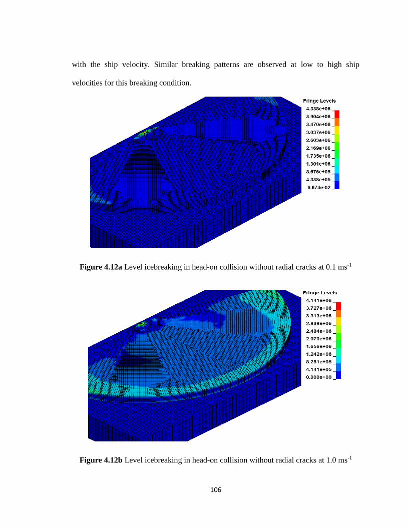
106

with the ship velocity. Similar breaking patterns are observed at low to high ship

velocities for this breaking condition.

Figure 4.12a Level icebreaking in head-on collision without radial cracks at 0.1 ms-1

Figure 4.12b Level icebreaking in head-on collision without radial cracks at 1.0 ms-1

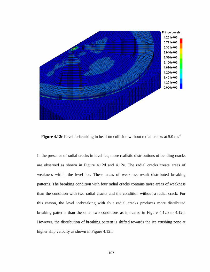
107

Figure 4.12c Level icebreaking in head-on collision without radial cracks at 5.0 ms-1

In the presence of radial cracks in level ice, more realistic distributions of bending cracks

are observed as shown in Figure 4.12d and 4.12e. The radial cracks create areas of

weakness within the level ice. These areas of weakness result distributed breaking

patterns. The breaking condition with four radial cracks contains more areas of weakness

than the condition with two radial cracks and the condition without a radial crack. For

this reason, the level icebreaking with four radial cracks produces more distributed

breaking patterns than the other two conditions as indicated in Figure 4.12b to 4.12d.

However, the distribution of breaking pattern is shifted towards the ice crushing zone at

higher ship velocity as shown in Figure 4.12f.

108

Figure 4.12d Level icebreaking in head-on collision with two radial cracks at 1.0 ms-1

Figure 4.12e Level icebreaking in head-on collision with four radial cracks at 1.0 ms-1

109

Figure 4.12f Level icebreaking in head-on collision with four radial cracks at 5.0 ms-1

Effect of Ship Velocity and Radial Cracks on Impact Force

The effect of ship velocity and radial cracks on the maximum impact force is plotted in

Figure 4.13 for three level icebreaking conditions. This figure indicates that the impact

force increases with the velocity but decreases with the number of existing radial cracks.

The level ice without a radial crack produces higher impact force for a given ship

velocity.

Figure 4.13 Impact force vs ship velocity for level icebreaking in head-on collision

0

50

100

150

200

250

300

350

400

0 1 2 3 4 5

Ship Velocity, ms-1

No

rmal

Imp

act

Fo

rce,

kN

No radial crack

Two radial cracks

Four radial cracks

110

4.3.3 Level Icebreaking in Shoulder Collision

For shoulder collisions, the failure patterns of level ice (1500 wedge) at an intermediate

ship velocity of 1 ms-1 are shown in Figures 4.14a and 4.14b. These figures indicate that

the failure pattern changes in the presence of existing radial cracks. In addition, the ice

wedge without a radial crack results higher impact force. The effect of ship velocity on

the impact force and bending crack pattern is similar to previously mentioned level

icebreaking condition of the head-on collision.

Figure 4.14a Level icebreaking in shoulder collision without radial cracks at 1.0 ms-1

111

Figure 4.14b Level icebreaking in shoulder collision with four radial cracks at 1.0 ms-1

4.4 Methodology to Formulate Dynamic Ice Load Models

There remains the need for better validation of the numerical results. Validation is not

easy due to the lack of specific type of full scale test data, where both local loads and

detailed ice observations are available. In addition, most of the existing analytical and

semi-empirical models are applicable to the static or quasi-static loading conditions.

Further testing is needed with a specific focus on local ice loads during operations in the

level ice.

This section describes a methodology to formulate four different dynamic ice load

models from the available analytical and semi-empirical models. In addition, two existing

112

breaking length models are presented to explore the velocity effect on the icebreaking

length. The formulated dynamic ice load models and presented breaking length models

will be used to validate the numerical model results.

Dynamic Ice Load Models

Two static ice load models and two dynamic factor models are selected from the existing

analytical and semi-empirical models in order to formulate the dynamic ice load models.

For the static ice load models, Kashteljan’s model in Eq. (3.4) and Daley’s proposed

model in Eq. (3.5) are considered. Both the models provide identical results for a given

ice wedge condition. Su et al. [14] mentioned that Kashteljan’s model results in a quite

small force value. Based on several experimental cases, a higher Cf value is suggested.

The Nguyen et al.’s model [32] used 4.5 for Cf as mentioned in Su et al. [14]. Therefore,

both Kashteljan’s model and Daley’s model are modified and multiplied with 4.5.

Daley and Kendrick [12] derived a dynamic factor (Kv) in terms of Froude Number (Fr)

to account for the velocity effect for a particular ice condition. The equations of Kv and

Fr are given as below:

𝐾𝑣 = 𝑚𝑎𝑥 {2.14 𝐹𝑟0.33

1}

(4.1)

𝐹𝑟 =𝑉 sin 𝛼 𝑐𝑜𝑠𝛽′

√𝑔ℎ

(4.2)

Lindqvist used a similar dynamic amplification factor for predicting the ice resistance

[22]. The dynamic factor proposed by Lindqvist is given in the following equation:

113

𝐾𝑣 = 1 + 1.4𝑉 sin 𝛼 𝑐𝑜𝑠𝛽′

√𝑔ℎ

(4.3)

The dynamic factors in Eqs. (4.1) and (4.3), and the modified static or quasi-static models

in Eqs. (3.4) and (3.5) are combined to produce four different dynamic ice load models.

These four dynamic ice load (Fdf ) models are given in Eqs. (4.4) to (4.7).

Modified Kashteljan static load with Daley dynamic factor model (MK-D model):

𝐹𝑑𝑓 = 4.5 (𝜃

𝜋)2

𝜎𝑓ℎ2. 𝑚𝑎𝑥 {2.14 𝐹𝑟

0.33

1}

(4.4)

Modified Daley static load with Daley dynamic factor model (MD-D model):

𝐹𝑑𝑓 = 𝐶𝑓𝜎𝑓ℎ2𝜃.𝑚𝑎𝑥 {2.14 𝐹𝑟

0.33

1}

(4.5)

Modified Kashteljan static load with Lindqvist dynamic factor model (MK-L model):

𝐹𝑑𝑓 = 4.5 (𝜃

𝜋)2

𝜎𝑓ℎ2. (1 + 1.4

𝑉 sin 𝛼 𝑐𝑜𝑠𝛽′

√𝑔ℎ)

(4.6)

Modified Daley static load with Lindqvist dynamic factor model (MD-L model):

𝐹𝑑𝑓 = 𝐶𝑓𝜎𝑓ℎ2𝜃. (1 + 1.4

𝑉 sin 𝛼 𝑐𝑜𝑠𝛽′

√𝑔ℎ)

(4.7)

The values of coefficient Cf in Eqs. (4.5) and (4.7) are 0.351, 0.438 and 0.585 for 300, 450

and 600 wedges, respectively.

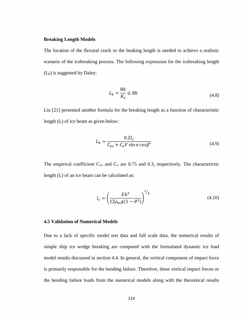
114

Breaking Length Models

The location of the flexural crack or the beaking length is needed to achieve a realistic

scenario of the icebreaking process. The following expression for the icebreaking length

(Lb) is suggested by Daley:

𝐿𝑏 =8ℎ

𝐾𝑣≤ 8ℎ

(4.8)

Liu [21] presented another formula for the breaking length as a function of characteristic

length (lc) of ice beam as given below:

𝐿𝑏 =0.2𝑙𝑐

𝐶𝑣𝑜 + 𝐶𝑣𝑉 sin 𝛼 𝑐𝑜𝑠𝛽′

(4.9)

The empirical coefficient Cvo and Cv are 0.75 and 0.3, respectively. The characterictic

length (lc) of an ice beam can be calculated as:

𝑙𝑐 = (𝐸ℎ3

12𝜌𝑤𝑔(1 − 𝜗2))

14⁄

(4.10)

4.5 Validation of Numerical Models

Due to a lack of specific model test data and full scale data, the numerical results of

simple ship ice wedge breaking are compared with the formulated dynamic ice load

model results discussed in section 4.4. In general, the vertical component of impact force

is primarily responsible for the bending failure. Therefore, these vertical impact forces or

the bending failure loads from the numerical models along with the theoretical results

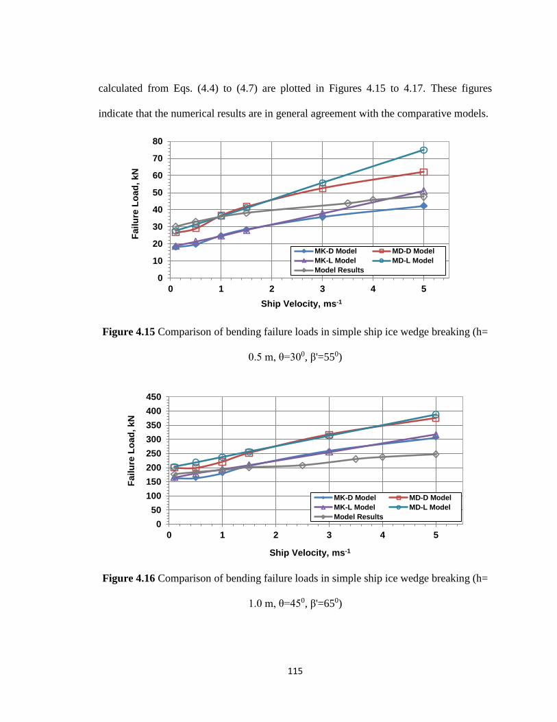
115

calculated from Eqs. (4.4) to (4.7) are plotted in Figures 4.15 to 4.17. These figures

indicate that the numerical results are in general agreement with the comparative models.

Figure 4.15 Comparison of bending failure loads in simple ship ice wedge breaking (h=

0.5 m, θ=300, β'=550)


1.0 m, θ=450, β'=650)

0

10

20

30

40

50

60

70

80

0 1 2 3 4 5

MK-D Model MD-D Model

MK-L Model MD-L Model

Model Results

Failu

reL

oad

, kN

Ship Velocity, ms-1

0

50

100

150

200

250

300

350

400

450

0 1 2 3 4 5



Model Results

Failu

reL

oad

, kN

Ship Velocity, ms-1

116


1.5 m, θ=600, β'=450)

The model icebreaking lengths for different icebreaking conditions along with the

theoretical breaking lengths are shown in Figures 4.18 and 4.19. These curves indicate

that the model breaking length does not match with the theoretical results exactly.

However, these curves follow a similar decreasing trend with the ship velocity.

Figure 4.18 Comparison of ice wedge breaking lengths in different models

0

200

400

600

800

1000

1200

1400

1600

1800

2000

0 1 2 3 4 5



Model Results

Failu

reL

oad

, kN

Ship Velocity, ms-1

0

2

4

6

8

10

12

14

0 1 2 3 4 5

Model: h=0.5m; β'=55deg; θ=30degModel: h=1.0m; β'=65deg; θ=45degModel: h=1.5m; β'=45deg; θ=60degDaley: h=0.5m; β'=55deg; θ=30degLiu: h=0.5m; β'=55deg; θ=30degDaley: h=1.0m; β'=65deg; θ=45degLiu: h=1.0m; β'=65deg; θ=45degDaley: h=1.5m; β'=45deg; θ=60degLiu: h=1.5m; β'=45deg; θ=60deg

Ship Velocity, ms-1

Bre

akin

g L

en

gth

, m

117

Chapter 5

Velocity Dependent Ice Flexural Failure Model

5.1 Introduction

This chapter presents an analytical closed form model of velocity dependent flexural

failure to predict the dynamic ice load from ship icebreaking process. The model is based

on numerical investigation of the ship icebreaking conducted in Chapter 4. The quality of

the model is checked against the numerical results considering different icebreaking

conditions and collision scenarios. The developed model is validated against full scale ice

impact test data and a non-linear dynamic bending load model. Application of the

velocity dependent flexural failure model to predict the bow impact load is demonstrated

for an example ship type (PC 1 ship). These bow impact load results are compared with

the IACS Polar Rules based results.

118

5.2 Velocity Dependent Flexural Failure Model

The comparison between the numerical and theoretical results in the previous chapter

indicated that the developed numerical models are well suited to predict the dynamic

impact force. These numerical models can be used for further ship icebreaking

investigations. The results from the numerical models have been used as the basis of a

new analytical closed form model for the velocity dependent force required to break an

ice wedge. Four factors; ship velocity, normal ship frame angle, ice thickness and ice

wedge angle are considered in this analysis. One factor at a time (OFAT) approach is

used to establish this empirical relationship between the ship velocity and impact force

for different icebreaking conditions. Equation (5.1) is the new flexural failure model of

vertical impact force for dynamic ice wedge breaking.

𝐹𝑣𝑑 = 0.29 𝑛0.7𝑘𝑣 𝜎𝑓 ℎ

2𝜃 (5.1)

where n is the number of wedge. The dynamic factor is defined as:

𝐾𝑣 = 1 + 2.57 sin 𝛼 cos 𝛽′ 𝜃0.2𝐹𝑟0.26 (5.2)

where Froude Number (Fr) is defined in Eq. (4.2). The normal impact force can be

expressed in the following form:

𝐹𝑛𝑑 =𝐹𝑣𝑑sin 𝛽′

(5.3)

In the new model, the flexural strength (σf) is assumed as linearly related to the impact

force similar to Eqs. (4.4) to (4.7). Hence, further investigation is needed to establish the

actual relationship between the flexural strength and impact force.

119

5.3 Comparison with Numerical Model

This section examines the quality and accuracy of the developed flexural failure model

against the numerical model results. The results from the developed model are compared

with numerical model results for different breaking conditions considering both the head-

on and shoulder collision scenarios. For simple ice wedge breaking in head-on collision,

the vertical impact force vs ship velocity curves of the flexural failure model along with

the numerical results are plotted in Figures 5.1 to 5.4. These curves illustrate the effect of

ice thickness, ice wedge angle and normal ship frame angle on the velocity dependent ice

failure load. The curves of the flexural failure model are well fitted with the numerical

model results. Therefore, the developed velocity dependent flexural failure model can be

used to explore the dynamic ship icebreaking process.


model for ice wedge breaking in head-on collision at different ice thicknesses (β'=650,

θ=300)

0

50

100

150

200

250

300

350

400

450

0 1 2 3 4 5

Num_model: h=1.5 m Flx_Model:h=1.5 mNum_model: h=1.0 m Flx_model: h=1.0 mNum_model: h=0.5 m Flx_model: h=0.5 m

Ship Velocity, ms-1

Failu

re L

oad

, kN

120


model for ice wedge breaking in head-on collision at different ice wedge angles (h=0.5

m, β'=650)


model for ice wedge breaking in head-on collision at different normal ship angles (h=0.5

m, θ=300)

0

20

40

60

80

100

120

0 1 2 3 4 5

Num_model: θ=60 deg Flx_model: θ=60 degNum_model: θ=45 deg Flx_model: θ=45 degNum_model: θ=30 deg Flx_model: θ=30 deg

Ship Velocity, ms-1

Failu

re L

oad

, kN

25

35

45

55

65

75

0 1 2 3 4 5

Num_model: β'=65 deg Flx_model: β'=65 degNum_model: β'=55 deg Flx_model: β'=55 degNum_model: β'=45 deg Flx_model: β'=45 deg

Ship Velocity, ms-1

Failu

re L

oad

, kN

121


model for ice wedge breaking in head-on collision with random breaking parameters

The developed flexural failure model can also be applied to the level icebreaking

scenario. Results from the flexural failure model are plotted with the numerical results in

Figures 5.5 to 5.7 for both collision scenarios. These figures indicate that the developed

model is well suited to the level icebreaking condition with and without any radial crack.


model for level icebreaking in head-on collision with and without radial cracks

0

200

400

600

800

1000

1200

1400

1600

0 1 2 3 4 5

Num_model: β'=65 deg, h=1 m, θ=45 deg, n=1

Flx_model: β'=65 deg, h=1 m, θ=45 deg, n=1

Num_model: β'=45 deg, h=1.5 m, θ=60 deg, n=1

Flx_model: β'=45 deg, h=1.5 m, θ=60 deg, n=1

Ship Velocity, ms-1

Fa

ilu

re L

oad

, kN

0

50

100

150

200

250

300

350

0 1 2 3 4 5

Num_No radial crack Flx_No radial crack

Num_Two radial cracks Flx_Two radial cracks

Num_Four radial cracks Flx_Four radial cracks

Ship Velocity, ms-1

Failu

re L

oad

, kN

122


model for level icebreaking in shoulder collision without radial cracks


model for level icebreaking in shoulder collision with four radial cracks

0

50

100

150

200

250

300

0 1 2 3 4 5

Num_ model

Flx_modelF

ailu

re L

oad

, kN

Ship Velocity, ms-1

0

20

40

60

80

100

120

140

0 1 2 3 4 5

Num_model

Flx_model

Failu

re L

oad

, kN

Ship Velocity, ms-1

123

5.4 Validation with Full Scale Test Data

In this section, the velocity dependent ice flexural failure model is validated against full

scale ice impact test data and against a finite element based non-linear dynamic bending

load model provided in Varsta [47].

In 1983, Rauma Shipyard conducted a full scale test with an artificial land craft bow in

order to investigate the effects of ship speed and frame angle on the ice load [47]. The

landing craft bow was installed at the front of the tug Rauma I. This makes the waterline

angle (α) equal to 900. A general arrangement of this ice impact test is shown in Figure

5.8.

Figure 5.8 Ice impact test arrangement indicating landing bow craft and ice wedge shape

[47]

124

In the test, the ice wedge was pre-sawned to achieve a controlled test condition. The

geometric dimensions of the ice wedge and the landing craft bow particulars are given in

Table 5.1. Further details of the test can be found in Varsta [47].

Table 5.1 Ice wedge geometry and landing craft bow particulars in full scale impact test

Parameters Values

Wedge edge length (lc) 3.5 m

Wedge depth (ld) 0.5 m

Wedge opening angle (θw) 450

Ice temperature on top surface (Ti) -2oC to -6.6oC

Waterline angle of landing bow (α) 900

Normal ship frame angle/striking angle (β') 300 (9 tests) and 500 (20 tests)

Varsta [47] developed a non-linear dynamic ice bending model based on the finite

element method. The model was further refined by comparing the above discussed full

scale test data. Varsta’s model assumed an average ice thickness of 0.35 m and ice

flexural strength of 1.2 MPa. The present study also considers these ice thickness and

flexural strength values for the validation purpose. In addition, the present study assumes

that the ice wedge forms an opening angle of 900 at the ship ice contact point instead of

flat contact edge which is the case with the Varsta’s model and full scale test. This

assumption is reasonable especially for the thinner ice where the flexural failure

dominates the ice failure process. Figure 5.9 indicates the assumed ice wedge geometry

along with the original ice wedge geometry.

125

Figure 5.9 Ice wedge geometry in full scale test (left), Varsta’s model (left) and present

model (right)

The full scale test data, Varsta’s model results and the velocity dependent ice flexural

failure model results are plotted in Figure 5.10. The figure indicates that the developed

velocity dependent ice flexural failure model provides almost identical results to Varsta’s

model for the normal ship frame angles of 300 and 500. These results are also in good

agreement with the full scale test data. At lower normal ship frame angle (250) some

differences are observed between the Varsta’s model and present model. However, no

full scale data is available at this ship frame angle to explain the differences.

126

Figure 5.10 Validation of velocity dependent ice flexural failure model with full scale

test data and Varsta’s model

5.5 Application to Bow Impact Load Estimation

The bow impact load is an essential component for the design ice load model, and hence

for the Polar ship design and safe speed methodology. The minimum ice failure load

from the flexural failure model and crushing failure model is the effective bow impact

load. Therefore, the bow impact load can be expressed as a function of the ice flexure

failure load (Ff) and the ice crushing load (Fc):

𝐹𝑏𝑜𝑤 = 𝑚𝑖𝑛 (𝐹𝑐 , 𝐹𝑓) (5.4)

0

0.1

0.2

0.3

0.4

0.5

0.6

0.7

0.8

0.9

0 0.5 1 1.5 2 2.5 3 3.5 4

Full Scale (50 deg)

Full Scale (30 deg)

Varsta Model (25 deg)



New Model (25 deg)

New Model (30 deg)

New Model (50 deg)

Ship Velocity, ms-1

No

rmal

Imp

act

Lo

ad

, M

N

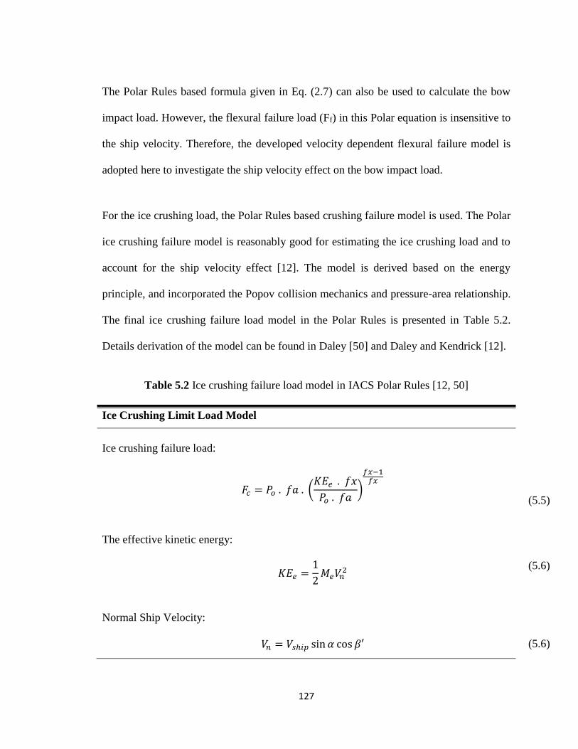
127

The Polar Rules based formula given in Eq. (2.7) can also be used to calculate the bow

impact load. However, the flexural failure load (Ff) in this Polar equation is insensitive to

the ship velocity. Therefore, the developed velocity dependent flexural failure model is

adopted here to investigate the ship velocity effect on the bow impact load.

For the ice crushing load, the Polar Rules based crushing failure model is used. The Polar

ice crushing failure model is reasonably good for estimating the ice crushing load and to

account for the ship velocity effect [12]. The model is derived based on the energy

principle, and incorporated the Popov collision mechanics and pressure-area relationship.

The final ice crushing failure load model in the Polar Rules is presented in Table 5.2.

Details derivation of the model can be found in Daley [50] and Daley and Kendrick [12].

Table 5.2 Ice crushing failure load model in IACS Polar Rules [12, 50]

Ice Crushing Limit Load Model

Ice crushing failure load:

𝐹𝑐 = 𝑃𝑜 . 𝑓𝑎 . (𝐾𝐸𝑒 . 𝑓𝑥

𝑃𝑜 . 𝑓𝑎)

𝑓𝑥−1𝑓𝑥

(5.5)

The effective kinetic energy:

𝐾𝐸𝑒 =1

2𝑀𝑒𝑉𝑛

2

(5.6)

Normal Ship Velocity:

𝑉𝑛 = 𝑉𝑠ℎ𝑖𝑝 sin 𝛼 cos 𝛽′ (5.6)

128

Effective Mass:

𝑀𝑒 =𝑀𝑠ℎ𝑖𝑝

𝐶𝑜

(5.7)

Coefficients:

𝑓𝑥 = 3 + 2𝑒𝑥

(5.8)

𝑓𝑎 = (tan 𝜃 2⁄

sin 𝛽′ cos2 𝛽′)

1+𝑒𝑥

(5.9)

The formula for mass reduction coefficient (Co) can be found in Daley [50]

This section investigates the ship velocity effect on the bow impact load during an ice

crushing process or an ice flexural failure process. For this reason, the equation (5.4) is

applied for a real ship type (PC 1) to calculate the bow impact load at different ship

velocities. The calculated bow impact load is compared with the Polar Rules based bow

impact load (Eq. 2.7) for a given ice thickness. Further, the ship velocity effect on the

bow impact load is also considered for different ice thicknesses. Finally, the bow impact

load is estimated using the Polar Rules specified parameters at different ship

displacements (mass). The principal particulars of the ship and ice wedges are listed in

Table 5.3.

129

Table 5.3 Principal particulars of ship and ice wedges for bow ice load

Parameters Value

Polar Class PC 1

Ship mass, M 10,000 tones

Ship block coefficient, Cb 0.768

Ship water plane coefficient, Cpw 0.7469

Ship mid-ship coefficient, Cm 0.934

Ship waterline angle, α 300

Normal ship frame angle, β' 460

Ice wedge angle, θ 1500

Flexural strength of ice, σf 0.58 MPa

For the given ice thickness of 1.5 m, the impact load vs ship velocity curves of different

models are plotted in Figure 5.11. These plotted models are the ice crushing model,

velocity dependent ice flexural failure model, bow impact load model (Eq. 5.4) and Polar

Rules based bow impact load model (Eq. 2.7). The ice crushing model indicates that the

impact load increases very quickly with the ship velocity, whereas a gradual change is

observed in the flexural failure model. For a particular ice condition, the ice crushing

model represents limiting impact load at slow ship velocity. For medium to higher ship

velocities, the flexural failure load is lower than the ice crushing load, and hence the

flexural failure model dominates the bow impact load for this velocity range. The new

bow impact load model in this figure indicates that there is a significant velocity effect in

130

the impact load at medium and higher ship velocities. This velocity effect is not included

in the Polar Rules model.

Figure 5.11 Ship velocity effect on bow impact load for an ice thickness of 1.5 m

Figure 5.12 is the result of the bow impact load model (Eq. 5.4) for a ship velocity range

of 0.1 ms-1 to 6 ms-1 at different ice thicknesses. The figure indicates that the crushing

failure dominates the resulting impact load for a wide range of ship velocity in the thicker

ice. In addition, crushing is also a dominating criterion for the slow velocity interaction

with the thinner ice. The figure also indicates that the flexure is the primary failure

criterion for the thinner ice at medium to higher ship velocities.

3286.2V1.3

0

500

1000

1500

2000

2500

3000

3500

4000

4500

5000

0 1 2 3 4 5 6 7

Bow Impact Load Ice Crushing Load

Ice Flexural Load Bow Impact Load (PC)

Ship Velocity, ms-1

Bo

w Im

pact

Lo

ad

, kN

131

Figure 5.12 Ship velocity effect on bow impact load at different ice thicknesses

Now, the bow impact loads for the PC 1 ship at different ship velocities and

displacements are estimated using the class dependent parameters such as the ice

thickness (7 m) and the flexural strength (1.4 MPa). These bow impact load results are

plotted in Figure 5.13 indicating the PC 1 design velocity (5.7 ms-1). The figure indicates

that the crushing is the only failure criterion at lower ship displacements ( 50 kT and 100

kT). For higher ship displacements from 150 kT to 250 kT, both the crushing and flexural

failure processes contribute to the bow impact loads.

100

1000

10000

100000

0 1 2 3 4 5 6

h=0.5 m h=1.0 m

h=1.5 m h=2 m

h=3 m h=4 m

h=5 m

Imp

act

Lo

ad

, kN

Ship Velocity, ms-1

132

Figure 5.13 Ship velocity effect on bow impact load at different ship displacements

The above discussion indicates that the Polar Rules based bow impact load estimation

method is reasonable for thicker ice operation, slow velocity interaction or for ships with

lower displacement. For thinner ice at medium to higher interaction velocities or the ship

with higher displacements, the Polar Rules based method may not be appropriate as their

flexural failure model is insensitive to the interaction velocity. Therefore, the developed

velocity dependent ice flexural failure model can help to enhance the Polar Rules based

design model to account for the velocity effect.

0

20

40

60

80

100

120

140

0 1 2 3 4 5 6

50 kT 100 kT150 kT 200 kT250 kT PC Design Velocity

Imp

act

Lo

ad

, M

N

Ship Velocity, ms-1

133

Chapter 6

Safe Speed Methodology for Polar Ships

6.1 Introduction

This chapter presents a safe speed methodology for the Polar ships. For this purpose, an

improved design ice load model is proposed based on the new velocity dependent ice

flexural failure model. The improved design ice load model is used to calculate the load

patch parameters. Further, the load patch parameters are employed to select the ship plate

and frame dimensions as well as to develop the safe speed methodology. The safe speed

methodology for the PC 5, PC 6 and PC 7 are demonstrated to examine the capability of

safe speed operation in different ice conditions. Finally, a software “Safe Speed Check

for Polar Ship” is developed which allows the easy prediction of ice load, the selection of

plate and frame dimensions, and the determination of safe speed limit for Polar ships.

134

6.2 Design Ice Load Model

Design ice load model is important for a safe speed methodology. The existing PC design

ice load model is based on the design scenario of glancing collision which is

characterized by the average pressure uniformly distributed over the rectangular load

patch [11]. This characterization of the design ice load or formulation of the rectangular

load patch requires the determination of several ice load parameters such as bow impact

load, line load, pressure and aspect ratio. For this purpose, the water line length of the

bow region is divided into four equal sub-regions [9-11]. The required ice load

parameters are calculated at the mid-position of each sub-region [11]. Figure 6.1

illustrates the methodology to estimate the design ice load parameters in the Polar Rules.

Figure 6.1 Design ice load formulation methodology in Polar Rules [9]

135

The magnitude of the bow impact force depends on the crushing failure and flexural

failure modes of the ice wedge. Therefore, the calculation of bow impact load requires

the ice crushing failure model and flexural failure model. The IACS Polar Rules specify

an additional limiting value of ice failure load. According to the Polar Rules, the bow

impact load cannot exceed this limiting value. The minimum of the ice crushing load,

flexural failure load and limiting failure load is considered as the bow impact load at a

particular bow region. Therefore, the bow impact load formula can be expressed as:

𝐹𝑖 = 𝑚𝑖𝑛 {

𝐹𝑐𝐹𝑓𝐹𝑙

}

(6.1)

where, Fi is the bow impact load; Fc is the ice crushing load; Ff is the flexural failure load

and Fl is the limiting ice failure load.

The ice crushing force (Fc) can be calculated from the IACS Polar crushing failure model

as given in Eq. (2.7) or Eqs. given in Table 5.2. The IACS Polar Rules proposed limiting

load formula in Eq. (2.7) can also be used to calculate the limiting ice failure load (Fl).

However, the IACS Polar flexural failure load model in Eq. (2.7) needs an alternative to

estimate the flexural failure load (Ff). This flexural failure model does not account for the

velocity effect. This velocity effect influences the bow impact load and hence the design

ice load model. Therefore, a modified model is presented for the bow impact load

calculation which includes the velocity effect on the flexural failure. In this modified

model, the Polar Rules based flexural failure model is replaced with the developed

velocity dependent flexural failure model.

136

The modified model for the bow impact load calculation at a particular position can be

expressed as:

𝐹𝑖 = 𝑚𝑖𝑛

{

𝐹𝑐 = (0.097 − 0.68(

𝑥

𝐿− 0.15)2

𝛼

√𝛽′𝐶𝐹𝑐𝐷

0.64

𝐹𝑓 =0.29𝑛0.7(1 + 2.57 𝑠𝑖𝑛 𝛼 𝑐𝑜𝑠 𝛽′ 𝜃0.2𝐹𝑟0.26)𝜎𝑓ℎ

2𝜃)

𝑠𝑖𝑛 𝛽′

𝐹𝑙 = 0.6𝐶𝐹𝑐𝐷0.64 }

(6.2)

The crushing class factor (CFc) is defined as:

𝐶𝐹𝑐 = 𝑃𝑜0.36𝑉𝑠

1.28 (6.3)

The ship velocity (Vs), ice thickness (h), ice strength (σf), nominal ice strength (Po) and

crushing class factor in Eqs. (6.2) and (6.3) are class dependent. For a particular Polar

ship, these parameters can be found from Table 6.1. Further, these parameters can be

used to estimate the bow impact load for a particular location (α, β and 𝑥

𝐿) and ship

displacement (D).

Table 6.1 Polar class dependent parameters for bow load calculation [9, 10]

Polar

Classes

Vs

m/s

Po

Mpa

h

m

σf

Mpa

CFc

PC 1 5.70 6.000 7.0 1.40 17.69

PC 2 4.00 4.200 6.0 1.30 9.89

PC 3 3.00 3.000 4.3 1.20 6.06

PC 4 2.50 2.450 3.5 1.10 4.50

PC 5 2.00 2.000 3.0 1.00 3.10

PC 6 1.75 1.500 2.8 0.70 2.40

PC 7 1.50 1.300 2.5 0.65 1.80

137

The next step after the bow impact load calculation is the estimation of load patch

parameters. For calculating the load patch aspect ratio (ARi), pressure (Pi), and line load

(Qi), Polar Rules based formulas given in the IACS [72] can be used for this purpose.

These rule based formulas are given in Eqs. (6.4) to (6.7).

Load patch aspect ratio:

𝐴𝑅𝑖 = 7.46 sin 𝛽′ ≥ 1.3 (6.4)

Pressure:

𝑃𝑖 = 𝐹𝑖0.22𝐶𝐹𝐷

2𝐴𝑅𝑖0.3 (6.5)

Line load:

𝑄𝑖 =𝐹𝑖0.61𝐶𝐹𝐷

𝐴𝑅𝑖0.35

(6.6)

The patch class factor is defined as [8]:

𝐶𝐹𝐷 = 𝑃𝑜0.389 (6.7)

Equations (6.2) and (6.6) are applicable to the bow area. For the non-bow region, the

impact force and line load can be calculated from Eqs. (6.8) and (6.10), respectively [72].

The impact load on the non-bow region is:

𝐹𝑛𝑜𝑛𝑏𝑜𝑤 = 0.36𝐶𝐹𝑐𝐷𝐹 (6.8)

The ship displacement factor is defined as:

138

𝐷𝐹 = {𝐷0.64 𝑖𝑓 𝐷 ≤ 𝐶𝐹𝐷𝐼𝑆

𝐶𝐹𝐷𝐼𝑆0.64 + 0.1(𝐷 − 𝐶𝐹𝐷𝐼𝑆) 𝑖𝑓 𝐷 > 𝐶𝐹𝐷𝐼𝑆

(6.9)

where, CFDIS is the displacement class factor.

The line load on the non-bow region is:

𝑄𝑛𝑜𝑛𝑏𝑜𝑤 = 0.639𝐹𝑛𝑜𝑛𝑏𝑜𝑤0.61 𝐶𝐹𝐷 (6.10)

Equations (6.2) to (6.10) can be used to obtain the design ice load parameters and the

rectangular patch load dimensions for both the bow region and non-bow region as shown

in Table 6.2.

Table 6.2 Design load patch particulars in IACS Polar Rules [7, 72]

Parameters Bow Area Non-bow Area

Design load width 𝑤𝑏𝑜𝑤 =

𝐹𝑏𝑜𝑤𝑄𝑏𝑜𝑤

𝑤𝑛𝑜𝑛𝑏𝑜𝑤 =𝐹𝑛𝑜𝑛𝑏𝑜𝑤𝑄𝑛𝑜𝑛𝑏𝑜𝑤

Design load height 𝑏𝑏𝑜𝑤 =

𝑄𝑏𝑜𝑤𝑃𝑏𝑜𝑤

𝑏𝑛𝑜𝑛𝑏𝑜𝑤 =𝑤𝑛𝑜𝑛𝑏𝑜𝑤3.6

Design Avg. Pressure 𝑃𝑎𝑣𝑔𝑏𝑜𝑤 =

𝐹𝑏𝑜𝑤𝑏𝑏𝑜𝑤𝑤𝑏𝑜𝑤

𝑃𝑎𝑣𝑔𝑛𝑜𝑛𝑏𝑜𝑤 =𝐹𝑛𝑜𝑛𝑏𝑜𝑤

𝑏𝑛𝑜𝑛𝑏𝑜𝑤𝑤𝑛𝑜𝑛𝑏𝑜𝑤

The peak pressure factor (PPFi) in Table 2.5 can be used in the design average pressure

equation to reflect the local peak pressure within the load patch. In addition, the hull area

factor (HFA) in Table 2.4 is used to estimate the ice load in different hull regions. Further

details of the ice load design process for the Polar ships can also be found in Daley [9],

Rahman [8] and IACS [72].

139

6.3 Plate and Frame Design

Plastic design criterion is adopted in the IACS Polar Rules for the plating and framing

requirements. This ensures better balance between the strength and safety margin against

the ultimate failure of the structure for a design ice load [68, 69]. Several limit state

equations were derived based on the plastic response of the plating and framing to meet

the rule based design criteria [68, 69].

For plating, the limit state equations are derived based on the plate folding mechanism

and by using the energy method [68]. These limit state equations specify the minimum

thickness required for the shell plating to resist the design ice load. The minimum

thickness requirement varies for different framing configurations and orientations. Table

6.3 contains the Polar Rules based minimum plate thickness equations for different

framing configurations and orientations.

In the Polar Rules, the frame is designed to maintain the minimum shear area and section

modulus [68, 69]. The limit state equations of the minimum shear area and section

modulus are derived based on three possible plastic collapse mechanisms [68, 69]. These

limit state equations are presented in Table 6.4 along with the limit load expressions.

Perhaps, the limit load expressions are used in the design process to predict the load

bearing capacity of the framing member. Detailed derivation and explanation of the limit

state equations can be found in Daley [69, 73] and Daley et al. [68].

140

Table 6.3 Minimum plate thickness for different framing configurations [72]

Shell Plate Requirements

Minimum shell plate thickness:

𝑡 = 𝑡𝑛𝑒𝑡 + 𝑡𝑐

Transversely-framed plating (Ω≥700):

𝑡𝑛𝑒𝑡 =

500𝑠√𝐴𝐹. 𝑃𝑃𝐹𝑃. 𝑃𝑎𝑣𝑔

𝑅𝑒𝐻

1 +𝑠2𝑏

Longitudinally-framed plating (Ω≤200and b≥s):

𝑡𝑛𝑒𝑡 =


𝑅𝑒𝐻

1 +𝑠2𝑙

Longitudinally-framed plating (Ω≤200 and b<s):

𝑡𝑛𝑒𝑡 =


𝑅𝑒𝐻. √2𝑏𝑠 − (

𝑏𝑠)

2

1 +𝑠2𝑙

For obliquely framed plating (700> Ω >200), linear interpolation is used.

where, Ω is the smallest angle between waterline and framing; s is the frame spacing;

ReH is the minimum nominal upper yield point and l is the distance between frame

supports. Details of the plating design can be found in IACS [72].

141

Table 6.4 Limit state equations in Polar Rules for framing [7, 68]

Limit State Equations

1st limit state – 3 hinge formation

Section modulus requirement:

𝑍𝑝 =𝑃. 𝑏. 𝑠. 𝑙

4. 𝜎𝑦(1 −

𝑏

2𝑙)

1

2 + 𝑘𝑤. [√1 − (𝐴𝑜𝐴𝑤)2

− 1]

Limit load:

𝑃𝑙𝑖𝑚𝑖𝑡_1 =(2 − 𝑘𝑤) + 𝑘𝑤√1 − 48𝑍𝑃𝑛𝑠(1 − 𝑘𝑤)

12. 𝑍𝑝𝑛𝑠𝑘𝑤2 + 1𝜎𝑦𝑍𝑝

4

𝑏. 𝑠. 𝑙. (1 −𝑏2𝑙)

2nd limit state: Shear panel formation

Section modulus requirement:

𝑍𝑝 =𝑃. 𝑏. 𝑠

𝜎𝑦. (1.1 + 5.75. 𝑘𝑧0.7). (1 −

𝑏

2𝑙) . 𝑙. [1 −

𝐴𝑤

2. 𝐴𝑜 (1 −𝑏2𝑙)]

Limit load:

𝑃𝑙𝑖𝑚𝑖𝑡_2 = [𝐴𝑤

√3+𝑍𝑝

𝑙. 𝑓𝑧] .

𝜎𝑦

𝑏 . 𝑠 (1 −𝑏2𝑙)

3rd Limit state: End Shear

Minimum web area: 𝐴𝑜 =1

2𝑃. 𝑏. 𝑠.

√3

𝜎𝑦

Limit load: 𝑃𝑙𝑖𝑚𝑖𝑡_3 =2.𝐴𝑜.𝜎𝑦

𝑏.𝑠.√3

Detailed description of minimum web area (Ao), web area (Aw), flange area (Af), flange

factor (kw), plastic modulus (Zp) and other parameters can be found in Daley et al. [68].

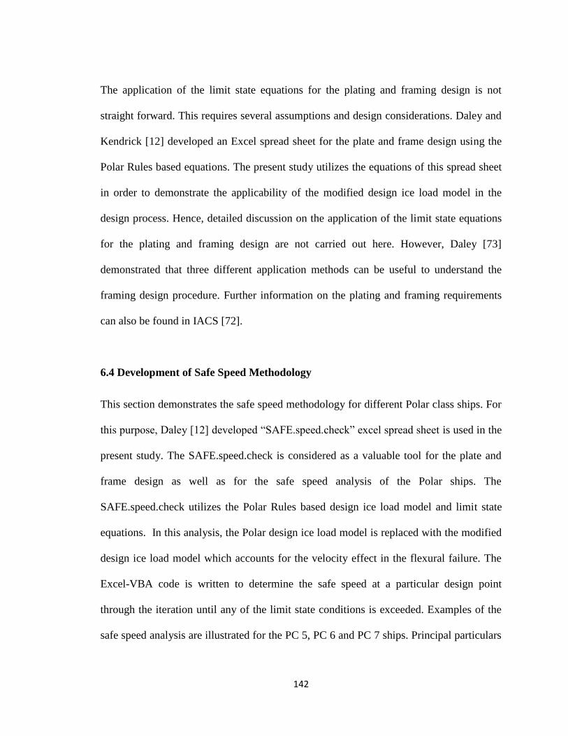
142

The application of the limit state equations for the plating and framing design is not

straight forward. This requires several assumptions and design considerations. Daley and

Kendrick [12] developed an Excel spread sheet for the plate and frame design using the

Polar Rules based equations. The present study utilizes the equations of this spread sheet

in order to demonstrate the applicability of the modified design ice load model in the

design process. Hence, detailed discussion on the application of the limit state equations

for the plating and framing design are not carried out here. However, Daley [73]

demonstrated that three different application methods can be useful to understand the

framing design procedure. Further information on the plating and framing requirements

can also be found in IACS [72].

6.4 Development of Safe Speed Methodology

This section demonstrates the safe speed methodology for different Polar class ships. For

this purpose, Daley [12] developed “SAFE.speed.check” excel spread sheet is used in the

present study. The SAFE.speed.check is considered as a valuable tool for the plate and

frame design as well as for the safe speed analysis of the Polar ships. The

SAFE.speed.check utilizes the Polar Rules based design ice load model and limit state

equations. In this analysis, the Polar design ice load model is replaced with the modified

design ice load model which accounts for the velocity effect in the flexural failure. The

Excel-VBA code is written to determine the safe speed at a particular design point

through the iteration until any of the limit state conditions is exceeded. Examples of the

safe speed analysis are illustrated for the PC 5, PC 6 and PC 7 ships. Principal particulars

143

for the ship and structure are chosen identical to Daley and Kendrick [12] as shown in

Table 6.5.

Table 6.5 Principal particulars of ship and structure for safe speed analysis

Parameters Value

Ship particulars:

Polar classes PC 5, PC 6 and PC 7

Ship displacement 50, 000 tones

Ship block coefficient, Cb 0.768

Ship water plane coefficient, Cpw 0.7469

Ship mid-ship coefficient, Cm 0.934

Ship waterline angle, α 300

Normal ship frame angle, β' 460

Structure particulars:

Frame orientation type Transverse

Yield strength of plate and frame, σyp and σyf 235 MPa

Young modulus of plate, Ep 207 GPa

Main frame span, a 2000 mm

Main frame spacing, s 350 mm

Waterline angle at contact points, αi 300, 220, 16.80, 12.550

Normal frame angle at contact points, , βi’ 460, 440, 350, 260

The safe speed methodology is developed in three stages. At first, the bow impact loads

at four different locations are calculated using Eq. (6.2). The maximum bow impact load

is used to determine the design load patch parameters using Eqs. (6.4) to (6.7) and

equations mentioned in Table 6.2. The calculated design load patch parameters for the PC

144

5, PC 6 and PC 7 are presented in Table 6.6. The table indicates that the upper Polar class

(PC 5) ship needs to be designed for higher impact force and the other patch load

parameters should be changed accordingly.

Table 6.6 Design load patch parameters for PC 5, PC 6 and PC 7

Patch Load Parameters PC 5 PC 6 PC 7

Max. bow impact load (MN) 14.482 9.372 6.871

Aspect ratio 5.369 5.369 5.369

Line load (MN/m) 3.723 2.552 2.013

Pressure (MPa) 5.139 3.730 3.115

Load patch width (m) 3.890 3.673 3.413

Ice load patch height (m) 0.724 0.684 0.646

The load patch parameters calculated in Table 6.6 are used to design the plate and frame

for the example Polar ships. The IACS Polar limit state equations in Table 6.4 and the

basic rule formulas given in Daley [73] are utilized in this design process. The modified

excel spread sheet and software (as discussed in section 6.5) automatically offer the

optimum plate thickness and frame type based on the load patch parameters. The offered

plate and frame dimensions and particulars for the PC 5, PC 6 and PC 7 are given in

Table 6.7. The excel spread sheet data for the PC 5, PC 6 and PC 7 are given in Appendix

C indicating detailed calculation of parameters and particulars related to the ice load

patch, plate and frame design.

145

Table 6.7 Offered plate and frame dimensions for PC 5, PC 6 and PC 7

Plate & Frame Particulars PC 5 PC 6 PC 7

Thickness of plate (mm) 28.00 23.50 21.50

Frame description F 380 x 27 F 320 x 24 HP 320x16.0

Height of web (mm) 380.00 320.00 285.96

Thickness of web (mm) 27.00 25.00 16.00

Width of flange (mm) - - 62.00

Thickness of flange (mm) - - 34.04

Finally, the Polar ships with the offered plates and frames are examined to check the safe

speed capability in different ice thicknesses. This involves the development of the “safe

speed vs ice thickness” curves. The safe speed analysis is performed for an ice thickness

range from 2.0 m to 3.5 m. Figures 6.2, 6.3 and 6.4 are the safe speed curves for the PC 5,

PC 6 and PC 7, respectively.

Figure 6.2 Safe speed curve for PC 5 ship

0

5

10

15

20

25

2 2.2 2.4 2.6 2.8 3 3.2 3.4 3.6

Safe

S

peed

[kn

ots

]

Ice Thickness [m]

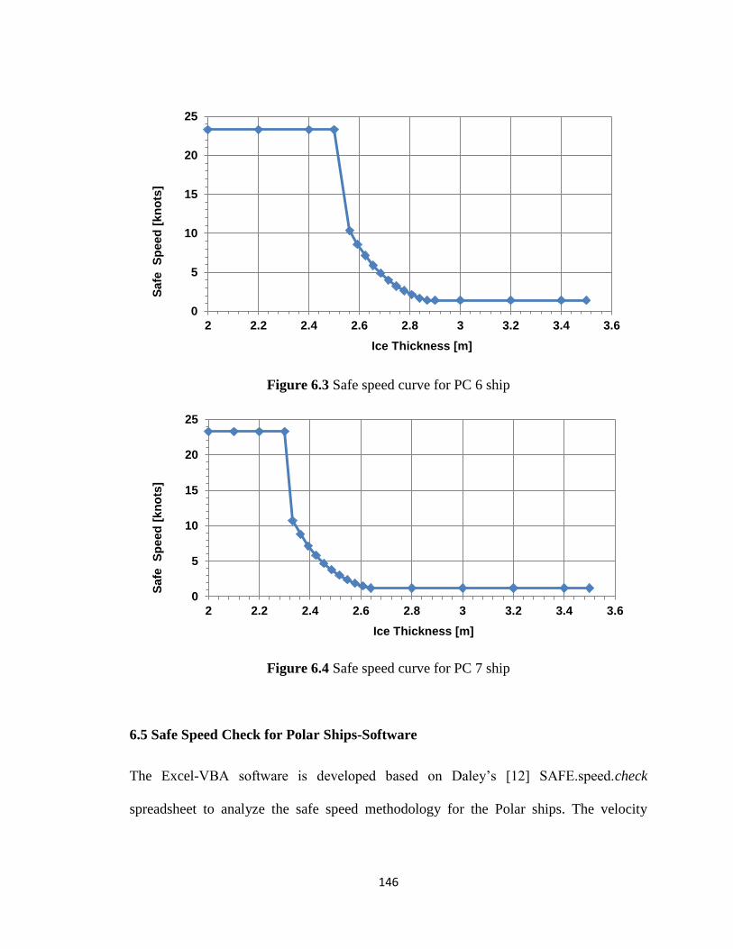
146



6.5 Safe Speed Check for Polar Ships-Software

The Excel-VBA software is developed based on Daley’s [12] SAFE.speed.check

spreadsheet to analyze the safe speed methodology for the Polar ships. The velocity

0

5

10

15

20

25

2 2.2 2.4 2.6 2.8 3 3.2 3.4 3.6

Safe

S

peed

[kn

ots

]

Ice Thickness [m]

0

5

10

15

20

25

2 2.2 2.4 2.6 2.8 3 3.2 3.4 3.6

Safe

S

peed

[kn

ots

]

Ice Thickness [m]

147

dependent flexural failure model is adopted into the software, and the software is named

as “Safe Speed Check for Polar Ships” (Figure 6.5). In addition to safe speed analysis, the

software allows easy estimation of the ice load, and plate and frame design as indicated in

the main menu of the software (Figure 6.6). The software permits working in excel

environment as well.

Figure 6.5 “Safe speed check for Polar ships” software

Figure 6.6 Main features of “Safe speed check for Polar ships” software

148

The effect of ship velocity, ship shape and ice condition can be investigated through the

“Ice Load Model” option. In addition, this option can be used to estimate the design ice

load parameters. On the other hand, “Plate and Frame” and “Safe Speed” options provide

the optimum plate and frame design, and safe speed analysis, respectively. Applications

of each option are demonstrated here with examples.

Ice Load Model Option

A 10,000 tones Polar ship (PC 7) is considered to illustrate the application of “Ice Load

Model” option. This option requires several ship and ice parameters for predicting the ice

load and ship velocity effect as indicated in Figure 6.7.

Figure 6.7 Ship and ice input parameters for ice load prediction

149

The above input parameters can be used to predict the bow ice load at a particular ice

thickness and ship velocity (Figure 6.8). Both the IACS Polar Rules model and the

modified model (Sazidy model) are utilized for this prediction. The IACS Polar Rules

model provides the ice crushing load, static flexural failure load and limit bow load. The

modified model allows the prediction of dynamic factor and dynamic flexural failure load

in addition to the ice crushing, static flexural failure and limit bow loads. The modified

model can also be used to determine the ice load patch parameters.

Figure 6.8 Bow ice load prediction at a particular ice thickness and ship velocity

The “Ice Load Model” option allows the investigation of ship velocity effect on the ice

crushing load, ice flexural failure load and bow limit load as shown in Figures 6.9 to

6.13. The velocity effect on the ice load for a range of ice thickness can also be studied

using both the Polar Rules based model and modified model (Sazidy model). Figures

6.14 and 6.15 represent the velocity effect on the bow limit load for different ice

thicknesses using these two models.

150

Figure 6.9 Investigation of ship velocity effect on bow ice load

Figure 6.10 Ship velocity effect on ice crushing load at 1 m thick ice

151

Figure 6.11 Ship velocity effect on ice flexural failure load at 1 m thick ice

Figure 6.12 Ship velocity effect on limit bow impact load at 1 m thick ice

Figure 6.13 Velocity effect on ice crushing, flexural and bow ice load at 1 m thick ice

152


m (Sazidy model)


m (Polar Rules model)

153

Plate and Frame Option

This option in the software is used to design the plate and frame for the Polar ships. This

design procedure needs the user to specify the contact angles at four bow locations to

formulate the design ice load model. Based on this design ice load model and structural

limit state equations, the software offers optimum plate thickness and frame dimensions.

Figure 6.16 indicates the offered plating and framing for a 50, 000 tones PC 5 ship.

Figure 6.16 Plate and frame design for a 50,000 tones PC 5 ship

Safe Speed Option

This option is used to analyze the safe speed capabilities of different Polar class ships.

Initially, the plate and frame are designed against specific design points. The designed

154

plate and frame are used for the safe speed analysis. The safe speed results and curves for

the 50, 000 tones PC 5 ship are presented in Figures 6.17 and 6.18.

Figure 6.17 Safe speed analysis for 50,000 tones PC 5 ship

Figure 6.18 Safe speed curve for 50,000 tones PC 5 ship

155

Chapter 7

Summary and Recommendations

7.1 Introduction

Previous studies indicate that the safe speed methodology can be a valuable tool to ensure

safe ship operation in the Polar water. The IMO, classification societies and ship

industries have shown their interest towards the development of safe speed methodology.

The main motivation of this present work is to help in improving the development of safe

speed methodology for the Polar ships. For this purpose, a velocity dependent flexural

failure model is developed and utilized to formulate the safe speed methodology for

different Polar class ships. The developed model represents significant improvement of

the Polar Rules based flexural failure model. The present research carries out several

tasks to develop the velocity dependent flexural failure model and safe speed

methodology. This chapter summarizes and evaluates these tasks. This chapter also

includes original contributions of the thesis along with the limitations and some guide

lines for future work.

156

7.2 Summary of Present Work

The following tasks are carried out to develop the velocity dependent flexural failure

model and safe speed methodology:

7.2.1 Study of Ship-Ice Interaction Process

Ship-ice interaction process is important to formulate the ice load model, and hence for

the Polar ship design practice and safe speed methodology. For this reason, the

fundamental theories and modeling efforts are reviewed in order to identify the critical

issues involved in the ship-ice interaction process. Emphasis has been placed on the

current understanding of the ice failure process, ship-ice interaction process and ship-ice

interaction modeling approaches. The effects of different influencing factors such as ship

velocity, ship hull shape, ice condition and water foundation on the interaction process

are investigated.

Most of the studies idealize the ship-ice interaction process based on the observation of

model scale and full scale tests. An idealized ship-ice interaction process consists of

breaking phase, rotating phase and sliding phase. The investigation of entire interaction

process considering all phases is important for the global ice force and ice resistance.

Studies indicate that the local peak force is responsible for the ship structural damage.

The breaking phase of ship-ice interaction is sufficient to extract this local peak force.

Hence, the present study considered only the breaking phase of ship-ice interaction.

157

The ship icebreaking process mainly involves the ice crushing and flexural failures which

are influenced by the water foundation underneath of a floating ice sheet. The icebreaking

pattern is important to explore this ship icebreaking process. Different idealized

icebreaking patterns are used to study the icebreaking process indicating the formation of

radial and circumferential cracks which produce several ice wedges or ice cusps. Many

researchers suggest modeling of simple ice wedge breaking instead of full ice sheet

especially for the local contact force.

Several attempts have been made to study the ship-ice interaction process analytically

and numerically. The existing analytical models or numerical models using the analytical

or semi-empirical approaches mainly focus on the prediction of global ice forces and ice

resistance for the continuous icebreaking and maneuvering operations. Most of these

models are over simplified and ignore one or more influencing parameters.

Advanced numerical techniques have also been employed to investigate the dynamic

bending behavior of ice in the ship-ice interaction. Most of these models are applied to

specific test conditions and cannot be used for the present investigation. Different

numerical methods such as FEM, CEM, DEM and XFEM, and different numerical

solvers such as Lagrangian, ALE and SPH are employed for these modeling purposes.

Many of these methods and solvers have the capability to generate the bending crack

initiation and propagation. However, the finite element method, with the element erosion

technique and the Lagrangian solver, is efficient and hence adopted in this study.

158

7.2.2 Material Models of Ice and Water

Material models play a vital role in characterizing the ship icebreaking process. For this

reason, three individual tests are conducted in the commercial software package LS

DYNA to select the material models and parameters for the ice crushing behavior, ice

flexural behavior and water foundation effect.

For the ice crushing behavior, an ice crushing test is performed in which the ice wedge is

modeled as an elastic-perfectly plastic material. The material model

*MAT_PLASTIC_KINEMATIC is used to represent this behavior. The compressive

strength and Young’s modulus of the crushing model are tuned to establish a similar

pressure-area relationship suggested in the Polar Rules for PC 1.

The four point bending test is conducted at quasi-static condition to represent the flexural

behavior. An isotropic elasto-plastic material model

*MAT_PLASTICITY_COMPRESSION_TENSION is considered for the ice beam. The

model considers different responses in compression and tension. In addition, the model

accounts for the strain rate sensitivity. The Element Erosion Method is employed in

which the effective plastic strain value is adjusted to get the proper bending response. The

model results are compared with the theoretical bending load and crack location.

Simple foundation tests are conducted to consider the water foundation effect. In the test,

the foundation is assumed as a linear elastic material, and modeled with the

159

*MAT_ELASTIC. The dimensions and elastic modulus are adjusted to match as close as

possible to the hydrostatic pressure of water on the lower ice surface.

7.2.3 Numerical Model of Ship Icebreaking

The numerical models of ship icebreaking process are developed to explore the velocity

effect on the ice flexural failure. The material models of the ice crushing, ice flexural

failure and water foundation effect are incorporated into these ship icebreaking models.

The numerical models of ship icebreaking consider two collision scenarios. One is the

head-on collision with a flat inclined face of the ship, and another is the shoulder

collision with an R-Class icebreaking ship. For the head-on collision, two breaking

conditions are considered; an ice wedge breaking and a level icebreaking. The shoulder

collision is only investigated for the level icebreaking. For the ice wedge breaking, the

effect of ship velocity on the breaking process is investigated for different ship angles, ice

wedge angles and ice thicknesses. The level icebreaking is investigated with and without

existing radial cracks for three different breaking conditions.

The model results indicate that the ice edge crushes for all breaking conditions. The

circumferential bending crack initiates and propagates in the bending zone. For a

particular ship frame angle, ice thickness and ice wedge; the bending crack location shifts

towards the ice crushing zone at higher ship velocity. These results also indicate that the

impact force, bending crack location and breaking pattern are influenced by the wedge

angle, ice thickness, normal ship frame angle and ship velocity.

160

For the level icebreaking in both collision scenarios, the bending failure occurs close to

the ice crushing zone in the absence of any radial crack. The location of the bending

crack does not change significantly with the ship velocity. More realistic distributions of

the bending cracks are observed in the presence of radial cracks. The distribution of

bending cracks is shifted towards the ice crushing zone at higher ship velocity. The

impact force increases with the ship velocity but decreases with the number of existing

radial cracks.

7.2.4 Formulation of Dynamic Ice Load Models

In the absence of any suitable dynamic ice load model, a simple methodology is

presented to formulate four dynamic ice load models based on the existing analytical and

semi-empirical models. Two static ice load models and two dynamic factor models are

selected. For the static ice load models, Kashteljan’s model [29] and Daley’s model [12]

are considered, and modified to meet Nguyen et al.’s [32] experimental observation [8].

Daley and Kendrick [12] derived, and Lindqvist proposed [22] dynamic factor models are

used in this analysis.

In addition to these four dynamic ice load models, two breaking length formulas are used

to validate the numerical model results. These results indicate that the numerical models

are in general agreement with the comparative models.

161

7.2.5 Velocity Dependent Ice Flexural Failure Model

An analytical closed form model of velocity dependent flexural failure is proposed to

predict the dynamic impact load from the ship icebreaking process. The model is

developed based on the numerical results of ship icebreaking process. Four factors; ship

velocity, ship angle, ice thickness and ice wedge angle are considered. One factor at a

time (OFAT) approach is used to establish this empirical relationship between the ship

velocity and the impact force for different icebreaking conditions.

The developed velocity dependent ice flexural failure model is validated against full scale

ice impact test data and against a finite element based non-linear dynamic bending load

model provided by Varsta [47]. The developed model results are in good agreement with

Varsta’s model results as well as with the full scale test data.

Application of the velocity dependent flexural failure model to predict the bow impact

load is also demonstrated for an example ship type (PC 1 ship). These bow impact loads

are compared with the IACS Polar Rules based results. The bow impact load analysis

indicates that there is a significant velocity effect in the impact load at medium and

higher ship velocity which is ignored in the Polar Rules based model. Therefore, the

developed velocity dependent flexural failure model represents a useful improvement of

the current Polar Rules based model.

162

7.2.6 Safe Speed Methodology

Safe speed methodology for different Polar class ships such as PC 5, PC 6 and PC 7 are

demonstrated to examine the capability of safe speed operation in different ice conditions.

For this purpose, a modified design ice load model is proposed based on the new velocity

dependent ice flexural failure model. This design ice load model is used to calculate the

ice load patch parameters. The ice load patch parameters along with the Polar Rules

based structural limit state equations are employed to design the plate and frame for the

safe speed methodology. Finally, the Excel-VBA software “Safe Speed Check for Polar

Ships” is developed which provides an easy and convenient way to predict the ice load on

the ship hull, design the plate and frame, analyze the safe speed capabilities of the Polar

ships.

7.3 Contributions of Present Work

The main goal of this research work is to develop a velocity dependent flexural failure

model to help in improving the Polar ship design and safe speed methodology. Several

tasks are carried out as mentioned in the previous section to accomplish this goal. These

tasks contribute to the engineering knowledge in many ways. The contributions of this

present work are addressed below:

Contribution 1: Ship-Ice Interaction Study

The literature review on ship-ice interaction process is useful to understand the basic

mechanisms, and to identify the critical issues involved in the process. Discussion on the

existing modeling approaches is helpful in selecting suitable modeling techniques and

163

methods for a particular ship-ice interaction scenario. This information provides a

previously un-collated guide to modeling local contact mechanisms as well as the global

ship-ice interaction.

Contribution 2: Material Model of Ice Flexural Failure

Ice flexural behavior is difficult to simulate. Studies indicate that the available numerical

material models of ice flexure are not suitable to capture all important features. In most

previously available cases, the models are oversimplified or follow a complicated

procedure to estimate the input parameters. Some of these models are unable to simulate

the bending crack initiation and propagation. In this study, a new and relatively simple

methodology is presented to develop a material model of ice flexural failure, based on a

four point bending test. This model allows more realistic investigation of the ice flexural

behavior in the ship-ice interaction as well as the larger ice-structure interaction problem.

It has proved its capability to produce the bending crack effectively which is important to

represent the ice flexural behavior.

Contribution 3: Material Models of Ice crushing and Water Foundation

Previous research indicates that existing material models can be used to represent the ice

crushing behavior and water foundation. However, these models are computationally

inefficient when they are utilized in a large and complicated model such as ship-ice

interaction model. In the present work, alternative simpler material models are developed

to characterize and simulate the ice crushing and water foundation effect at lower

164

computational cost and with equal fidelity. These material models along with the ice

flexural failure models can be used to investigate different ice interaction problems.

Contribution 4: Numerical Models of Ship Icebreaking

Numerical models of ship icebreaking are valuable tools to predict the ice impact load on

the ships and offshore structures. The models developed in the present work allow a

complicated ship-ice interaction process to be modeled using simple methodology and

procedure. These models consider ice edge crushing, ice flexural failure and water

foundation effect. The consideration of these principal mechanisms is not previously

observed in published finite element models. The developed numerical models utilize an

Element Erosion Method (EEM) which overcomes the difficulties of generating bending

crack initiation and propagation. The models are well suited to study the dynamic ship-

ice interaction process, and to investigate the effect of ship velocity, ship shape and ice

condition on the icebreaking pattern.

Contribution 5: Investigation of Level Icebreaking

In this research, emphasis is placed on the modeling of ship and ice wedge breaking

based on the local contact mechanism. However, a simple methodology is presented to

investigate level icebreaking using the numerical models of ship icebreaking. The present

work demonstrates how an existing radial crack might affect the level icebreaking pattern

and icebreaking force. The methodology creates a scope for future research on the

continuous icebreaking and prediction of ice resistance which involves the level

icebreaking.

165

Contribution 6: Methodology to Formulate Dynamic Ice Load Models

Researchers and scientists always find difficulties in validating ship-ice interaction

models. In general, model scale and full scale test results are utilized to validate the

global ship-ice interaction models. Neither of these can characterize the local contact

mechanism between the ship and ice. Analytical models are more suitable for this

validation purpose. However, the existing analytical models are applicable to the static

ship icebreaking conditions. In the present work, an alternative method is introduced to

formulate four dynamic ice load models from existing static analytical and semi-

empirical models. The models are beneficial in the absence of model test data or field test

data.

Contribution 7: Velocity Dependent Flexural Failure Model

The velocity dependent flexural failure model is developed in an innovative way, using

the numerical models of basic ship icebreaking mechanisms. The model is helpful to

study the effect of ship velocity, ship shapes and ice conditions on the icebreaking

process. This model incorporates the velocity effect in ship icebreaking and provides

significantly improved load predictions when compared to the IACS Polar Rules based

model, and Daley and Kendrick model [12], especially for the thinner ice and higher ship

speed operation. This velocity dependent flexural failure model as well as the numerical

models can be used in exploring different collision scenarios.

Contribution 8: Analysis of Bow Impact Load

Bow impact load analysis is carried out using the velocity dependent flexural failure

model for the Polar class ships. This analysis incorporates and explores the ship velocity

166

effect on the bow impact load, which is important to formulate design load patch

parameters. Improved load patch definition is useful in plate and frame design, Polar ship

design practice and safe speed methodology.

Contribution 9: Safe Speed Check for Polar Ships

This software provides a safe speed methodology for different Polar class ships. This is a

first implementation for Polar ships of rationally based safe operational guidance that can

be used on the bridge of a vessel. In addition to the operational safe speed methodology,

the software provides an easy estimation of design ice loads, and simple design of ship

plates and frames that can be used at the design stage based on operational scenarios.

7.4 Limitations of Present Work

In this present work, several assumptions and simplifications are made to achieve the

research objectives. In some cases, limitations need to be addressed for future refinement

and improvement of the work. Some of these assumptions and major limitations are

discussed below:

The variation or influence of different ice properties such as Young modulus,

density, flexural strength, compressive strength which are not considered in the

development of ice material models.

Material models of ice crushing and water foundation provide equivalent ice

crushing force and hydrodynamic force, respectively. However, these models do

not simulate the true crushing behavior and water foundation effect.

167

Numerical models of ship icebreaking do not account for friction between the ship

hull and ice.

Numerical models are suitable to study the local contact mechanism of

icebreaking phase. These models are not applicable to the global ship-ice

interaction problem.

Numerical models can also be applied to investigate the local contact between the

ship and level ice. However, these models cannot be used in exploring continuous

level icebreaking.

Due to the lack of specific test data, numerical model results are validated against

the existing analytical models.

Numerical models of level icebreaking consider already existing radial cracks.

These models are not able to simulate the radial crack initiation and propagation.

The velocity dependent flexural failure model assumes that the flexural load is

proportional to the flexural strength.

Presented safe speed methodology ignores many influencing factors. This is based

on only the ice crushing and ice flexural failure models. This methodology can be

termed as technical safe speed.

168

7.5 Recommendations for Future Work

Based on above assumptions and limitations, following refinements and improvements of

the work are recommended for future investigation:

Parameter sensitivity study focusing on the ice properties such as Young modulus,

density, compressive strength, flexural strength etc.

Improvement of the ice crushing and water foundation material models for more

realistic behaviors

Refinement of the numerical models considering ship-ice friction

Extension of the numerical models to investigate the global ship-ice interaction

and continuous level icebreaking

Development of improved numerical model to simulate the radial crack initiation

and propagation. More investigation is needed to explore the effects of radial

crack on the level icebreaking

Numerical investigation of different ice collision scenarios rather than shoulder

collision and head-on collision

Improvement of the velocity dependent flexural failure model by exploring the

rate sensitivity of flexural strength and crushing strength. More investigation is

needed to explore the velocity effect on the ice crushing and flexural failure.

Improvement of the developed safe speed methodology considering different

influencing factors

169

References

[1] Arctic Council, 2009, “Arctic Marine Shipping Assessment”, Report on Arctic

Marine Shipping.

[2] Kubat, I. and Timco, G., 2003, “Vessel Damage in the Canadian Arctic”, Proceedings

17th International Conference on Port and Ocean Engineering under Arctic Conditions,

POAC'03, 1, pp. 203-212, 2003-06-16.

[3] Likhomanov, V., Timofeev, I. Stepanov, Kastelyan, V., Iltchuk, A., Krupina, N. and

Klenov, A., 1997, “Scientific Basis and Methodology of the Development of an Ice

Passport”, Report Prepared for Arctic and Antarctic Research Institute Department of

Ship Performance in Ice, St. Petersburg, Russia.

[4] Shunying, J. and Shewen, L., 2012, “Interaction between Sea Ice/Iceberg and Ship

Structures: A Review”, Advances in Polar Science, 23: 187-195, doi:

10.3724/SP.J.1085.2012.00187.

[5] Sawamura, J., Riska, K. and Moan, T., 2009, “Numerical Simulation of Breaking

Patterns in Level Ice at Ship’s Bow”, Proceedings of the Nineteenth (2009) International

Offshore and Polar Engineering Conference, Osaka, Japan.

170

[6] Daley, C. G. and Colbourne, D. B., 2012, “Arctic Ocean Engineering-Course Notes”,

Memorial University of Newfoudland, St. John’s, NL, Canada.

[7] Dolny, J., Yu, H-C., Daley, C., Kendrick, A., 2013, “Developing a Technical

Methodology for the Evaluation of Safe Operating Speeds in Various Ice Conditions”,

Proceedings of the 22nd International Conference on Port and Ocean Engineering under

Arctic Conditions, Espoo, Finland.

[8] Rahman, M. M., 2012, “Structural Resistance of Polar Ships and FPSO´s to Ice

Loading”, M. Sc. Thesis, Norwegian University of Science and Technology, Department

of Marine Technology, Norway.

[9] Daley, C., n.d., “IACS Requirements for Polar Class Ships Overview and

Background”, www.engr.mun.ca/~cdaley/8674/L22aPolar%20Classes.ppt.

[10] Yu, H., 2008, “IACS Polar Class Requirements and Hull Structural Design

Applications”,http://legacy.sname.org/sections/texas/Meetings/2008/September%20Luncheo

n/SNAME-Texas%20Polar%20Class%20Rules%20-%20Han%20Yu.pdf.

[11] Germanischer Lloyd, 2008, “Rules for Classification and Construction-Ship

Technology”, Report on Guidelines for the Construction of Polar Class Ships.

171

[12] Daley, C. and Kendrick, A., 2011, “Safe Speed in Ice,” Final Report, Prepared for

BMT Fleet Technology, Reference: 6931DFR.Rev00, Ottawa, ON, Canada.

[13] Lubbad, R., and Loset, S., 2010, “A Numerical Model for Real-Time Simulation of

Ship-Ice Interaction,” Journal of Cold Regions Science and Technology, 65 (2011) 111-

127.

[14] Su, B., Riska, K., and Moan, T., 2009, “A Numerical Method for the Prediction of

Ship Performance in Level Ice,” Journal of Cold Regions Science and Technology, 60

(2010) 177-188.

[15] O’Connell, B. J., n.d., “Ice Hazard Radar”, http://www.dfo-

mpo.gc.ca/Library/343422.pdf

[16] Abraham, J., 2008, “Plastic Response of Ship Structure Subjected to Ice Loading”,

Master of Engineering Thesis, Memorial University of Newfoundland, St. John’s, NL,

Canada.

[17] Hänninen, S., 2003, “Incidents and Accidents in Winter Navigation in the Baltic Sea,

Winter 2002 – 2003”, Report for Winter Navigation Research Board,

http://www.trafi.fi/filebank/a/1352716465/5666a0c12549e09d1f84c3075353d3de/10732-

No_54_incidents_and_accidents_2003.pdf.

http://www.dfo-mpo.gc.ca/Library/343422.pdf

http://www.dfo-mpo.gc.ca/Library/343422.pdf

http://www.trafi.fi/filebank/a/1352716465/5666a0c12549e09d1f84c3075353d3de/10732-No_54_incidents_and_accidents_2003.pdf

http://www.trafi.fi/filebank/a/1352716465/5666a0c12549e09d1f84c3075353d3de/10732-No_54_incidents_and_accidents_2003.pdf

172

[18] Aksnes, V., 2010, “A Simplified Interaction Model for Moored Ships in Level Ice,”

Journal of Cold Regions Science and Technology, 63 (2010) 29-39.

[19] Su, B., 2013, “Maneuverability of Ships in Ice: Numerical Simulation and

Comparison with Field Measurements”, Presentation for the Research Council of

Norway, http://www.cesos.ntnu.no/attachments/078_S11_Biao%20Su.pdf.

[20] Riska, K., 2011, “Ship–Ice Interaction in Ship Design: Theory and Practice”, Article

on Research and Development Trend for Arctic Ship Design, http://www.arctis-

search.com/Ship-Ice+Interaction+in+Ship+Design+-+Theory+and+Practice.

[21] Liu, J., 2009, “Mathematical Modelling Ice-Hull Interaction for Real Time

Simulations of Ship Maneuvering in Level ice,” Ph.D. Thesis, Memorial University of

Newfoundland, St. John’s, NL, Canada.

[22] Skar, T., 2011, “Ice Induced Resistance of Ship Hulls: A Comparison of Resistance

Estimated from Measurements and Analytical Formulations,” Master Thesis, Norwegian

University of Science and Technology, Norway.

http://www.cesos.ntnu.no/attachments/078_S11_Biao%20Su.pdf

http://www.arctis-search.com/Ship-Ice+Interaction+in+Ship+Design+-+Theory+and+Practice

http://www.arctis-search.com/Ship-Ice+Interaction+in+Ship+Design+-+Theory+and+Practice

173

[23] Jeong, S., 2014, “A Semi-Empirical Method of Ice Resistance Prediction in Level

Ice”, International Conference and Exhibition on Performance of Ships and Structures in

Ice, Alberta, Canada, ICETECH14-141-RF.

[24] Tan, X., Su, B., Riska, K., and Moan, T., 2012, “The Effect of Heave, Pitch and Roll

Motions to Ice Performance of Ships”, Proceedings of the 21st IAHR International

Symposium on Ice, Dalian, China.

[25] Erceg, S., Ehlers, S., Polach, R. F. V. B. and Leira, B., 2014, “A Numerical Model to

Initiate the Icebreaking Pattern in Level Ice”, Proceedings of the ASME 2014 33rd

International Conference on Ocean, Offshore and Arctic Engineering, California, USA,

OMAE2014-23409.

[26] Myland, D. and Ehlers, S., 2014, “Theoretical Investigation on Ice Resistance

Prediction Methods for Ships in Level Ice”, Proceedings of the ASME 2014 33rd


OMAE2014-23304.

[27] Tan, X., Riska, K., and Moan, T., 2014, “Effect of Dynamic Bending of Level Ice on

Ship's Continuous-Mode Icebreaking”, Journal of Cold Regions Science and Technology,

106-107 (2014) 82-95.

174

[28] Tan, X., Su, B., Riska, K., and Moan, T., 2013, “A Six-Degrees-of-Freedom

Numerical Model for Level Ice–Ship Interaction”, Journal of Cold Regions Science and

Technology, 92 (2013) 1-16.

[29] Kashteljan, V. I., Poznyak, I. I., and Ryvlin, A. Y.,1968, “Ice Resistance to Motion

of A Ship”, Translation, Sudostroenie, Leningrad, Translation by Marine Computer

Application Corporation.

[30] Enkvist, E., 1972, “On the Ice Resistance Encountered by Ships Operating in the

Continuous Mode of Icebreaking”, The Swedish Academy of Engineering Sciences in

Finland, Helsinki, Report No. 24, 181 pp.

[31] Kotras, T. V., Baird, A.V., and Naegle, J. W., 1983, “Predicting Ship Performance in

Level Ice”, Trans. of Society of Naval Architects and Marine Engineers, Vol.91, p. 329-

349.

[32] Nguyen, D. T., Sørbø, A. H. and Sørensen, A. J., 2009, “Modelling and Control for

Dynamic Positioned Vessels in Level Ice”, Proceedings of 8th Conference on

Maneuvering and Control of Marine Craft, pp. 229–236, Guarujá, Brazil.

[33] Lu, W., Lubbad, R., Loset, S., and Hoyland, K., 2012, “Cohesive Zone Method

Based Simulation of Ice Wedge Bending: a Comparative Study of Element Erosion,

175

CEM, DEM and XFEM,” Proceedings of the 21st IAHR International Symposium on Ice,

Dalian, China.

[34] Sawamura, J., Tachibana, T., Tsuchiya, H., and Osawa, N., 2010, “Numerical

Investigation for the Bending Failure of Wedge-Shaped Floating Ice”, Proceedings of the

20th IAHR International Symposium on Ice. Lahti, Finland.

[35] Sawamura, J. Riska, K., and Moan, T., 2008, “Finite Element Analysis of Fluid-Ice

Interaction during Ice Bending”, Proceedings of the 19th IAHR International Symposium

on Ice, BC, Canada.

[36] Lindqvist, G., 1989, “A Straightforward Method for Calculation of Ice Resistance of

Ships”, Proceeding of the 10th International Conference on Port and Ocean Engineering

under Arctic Conditions (POAC), Lulea, Sweden, p. 722-735.

[37] Hoving, J., 2012, “Numerical Modelling of Ice & Ice-Structure Interactions”,

Presentation on Arctic Battle Symposium, Delft University of Technology, Netherlands,

[38] Daley, C. and Riska, K., 1995, “Conceptual Framework for an Ice Load Model”,

Report Prepared for National Energy Board, Calgary, Alberta,

http://www.engr.mun.ca/~cdaley/Documents/concept2.pdf.

http://www.engr.mun.ca/~cdaley/Documents/concept2.pdf

176

[39] Lau, M., 2006, “Discrete Element Modeling of Ship Maneuvering In Ice”,

Proceedings of the 18th IAHR International Symposium on Ice, Sapporo, Japan.

[40] Phillips, L. D., 1994, “Simulation of Ship-Ice Collision Dynamics”, Ph.D. Thesis,

Carleton Institute for Civil Engineering, Ottawa, Canada.

[41] Johnes, S. J., 2004, “Ships in Ice - A Review”, 25th Symposium on Naval

Hydrodynamics, St. John’s, NL, Canada.

[42] Runeberg, R., 1888/89, “On Steamers for Winter Navigation and Ice-breaking”,

Proceeding of Institution of Civil Engineers, Vol. 97, Pt. III, p. 277-301.

[43] Lewis, J. W. and Edwards, R. Y. J., 1970, “Methods for Predicting Icebreaking and

Ice Resistance Characteristics of Icebreakers”, Trans. of Society of Naval Architects and

Marine Engineers, Vol.78, p. 213-249.

[44] White, R. M., 1970, “Prediction of Icebreaker Capability”, Trans. of The Royal

Institution of Naval Architects (RINA), Vol. 112, No. 2, p. 225-251.

[45] Milano, V. R, 1973, “Ship Resistance to Continuous Motion in Ice”, Trans. of

Society of Naval Architects and Marine Engineers, Vol.81.

177

[46] Kheisin, D. E., Likhomanov, V. A. and Kurdyumov, V. A., 1975, "Determination of

Specific Breakup Energy and Contact Pressures Produced by the Impact of a Solid

against Ice", Symp. on Physical Methods in Studying Snow and Ice, Leningrad, CRREL

Translation TL539.

[47] Varsta, P., 1983, “On the Mechanics of Ice Load on Ships in level ice in the Baltic

Sea”, PhD Thesis, Technical Research Centre of Finland, Espoo, Finland.

[48] Valanto, P., 2001, “The Resistance of Ships in Level Ice”, Trans. of Society of Naval

Architects and Marine Engineers, Vol.109, p. 53-83.

[49] Liu, J., Lau, M. and Williams, F. M., 2006, “Mathematical Modeling of Ice-Hull

Interaction for Ship Maneuvering in Ice Simulations”, International Conference and

Exhibition on Performance of Ships and Structures in Ice, Alberta, Canada, ICETECH06-

126-RF.

[50] Daley, C., 1999, “Energy Based Ice Collision Forces,” Proceedings of the 15th

International Conference on Port and Ocean Engineering under Arctic Conditions,

Helsinki University of Technology in Espoo, Finland.

[51] Kerr, A. D., 1976, “The Bearing Capacity of Floating Ice Plates Subjected to Static

or Quasi-Static Loads”, Journal of Glaciology, Vol. 17, No. 76.

178

[52] Zhou, L., Su, B., Riska, K., and Moan, T., 2011, “Numerical Simulation of Moored

Ship in Level Ice”, Proceedings of the ASME 2011 30th International Conference on

Ocean, Offshore and Arctic Engineering, Rotterdam, Netherlands, OMAE2011-49115.

[53] Sawamura, J., Tsuchiya, H., Tachibana, T., and Osawa, N., 2010, “Numerical

Modeling for Ship Maneuvering in Level Ice”, Proceedings of the 20th IAHR

International Symposium on Ice. Lahti, Finland.

[54] Ehlers, S., and Kujala, P., 2013, “Optimization-Based Material Parameter

Identification for the Numerical Simulation of Sea Ice in Four-Point Bending,” Journal of

Engineering for the Maritime Environment, 0(0) 1-11.

[55] Pernas-Sanchez, J., Pedroche, D.A., Varas, D., Lopez-Puente, J. L., and Zaera, R.,

2012, “Numerical Modeling of Ice Behavior under High Velocity Impacts”, Department

of Continuum Mechanics and Structural Analysis, Universidad Carlos III de Madrid,

Madrid, Spain.

[56] Zong, R., 2012, “Finite Element Analysis of Ship-Ice Collision using LS-Dyna,” M.

Eng. Thesis, Memorial University of Newfoundland, St. John’s, NL, Canada.

[57] Daiyan, H., and Sand, B., 2011, “Numerical Simulation of the Ice-Structure

Interaction in LS-Dyna”, Proceedings of 8th European LS-DYNA Users Conference,

Strasbourg.

179

[58] Carney, K. S., Benson, D. J., DuBois, P., and Lee, R., 2006, “A Phenomenological

High Strain Rate Model with Failure for Ice”, International Journal of Solids and

Structures, 43 (2006) 7820-7839, 2006.

[59] Gürtner, A., Bjerkas, M., Kuhnlein, W., Jochmann, P. and Konuk, I., 2009,

“Numerical Simulation of Ice Action to A Lighthouse”, Proceedings of the ASME 2009

28th International Conference on Ocean, Offshore and Arctic Engineering, Honolulu,

Hawaii, OMAE2009-80164.

[60] Nevel, D. E., 1961, “The Narrow Free Infinite Wedge on Elastic Foundation”, U.S.

Army Cold Regions Research and Engineering Laboratory, Research Report 79, 24 pp.

[61] Shunying, J., Zilin, L., Chunhua, L. and Jie, S., 2013, “Discrete Element Modeling

of Ice Loads on Ship Hulls in Broken Ice Fields”, Acta Oceanologica Sinica, 32(11): 50-

58, doi: 10.1007/s13131-013-0377-2.

[62] Wang, B., Yu, H. and Basu, R., 2008, “Ship and Ice Collision Modeling and

Strength Evaluation of LNG Ship Structure”, Proceedings of the ASME 2008 27th

International Conference on Ocean, Offshore and Arctic Engineering, Estoril, Portugal,

OMAE2008-57134.

180

[63] Gagnon, R. E. and Wang, J., 2012, “Numerical Simulation of a Tanker Collision

with a Bergy Bit Invorporating Hydrodynamics, a Validated Ice Model and Damage to

the Vessel”, Journal of Cold Regions Science and Technology, 81 (2012) 26-35.

[64] Kim, H., 2014, “Simulation of Compressive ‘Cone-Shaped’ Ice Specimen

Experiments using LS-DYNA”, 13th LS-DYNA® International Conference, Michigan,

USA.

[65] Das, J., Polic, D., Ehlers, S. and Amdahl, J., 2014, “Numerical Simulation of an Ice

Beam in Four-Point Bending using SPH”, Proceedings of the ASME 2014 33rd


OMAE2014-23228.

[66] LS-Dyna, 2011, www.lstc.com.

[67] Akerstrom, F. B. W. C., 2012, “Ice Class Requirements on Side Shell Structures-A

Comparison of Local Strength Class Requirements Regarding Plastic Design of Ice-

Reinforced Side Shell Structures”, M. Sc. Thesis, Chalmers University of Technology,

Gothenburg, Sweden.

[68] Daley, C., Kendrick, A. and Appolonov, E. M., 2001, “Ships, Plating and Framing

Design in the Unified Requirements for Polar Class”, Port and Ocean Engineering Under

Arctic Conditions, POAC-01. Pp. 779-791.

http://www.lstc.com/

181

[69] Daley, C., 2002, “Derivation of Plastic Framing Requirements for Polar Ships”,

Journal of Marine Structures, 15 (2002) 543-559.

[70] CNIIMF, 2007, “Ice Certificate for 70000 Dwt Arctic Shuttle Tankers”, Report

Prepared for Central Marine Research and Design Institute, Saint-Petersburg.

[71] Makinen, E., Alekseyev, J., Frankenstein, G., Kitagawa, H., Maksutov, D.,

Michailidis, M., Milano, R. and Schwarz, J., 1984, “Review of Research on Modeling in

of Importance to the ITTC”, Report prepared for ITTC, pp. 592.

[72] IACS, 2011, “Requirements Concerning Polar Class”, Report of International

Association of Classification Societies.

[73] Daley, C. G., 2002, “Application of Plastic Framing Requirements for Polar Ships”,

Journal of Marine Structures, 15 (2002) 533-542.

[74] Popov, Y., Faddeyev, O., Kheisin, D. and Yalovlev, A., 1967, “Strength of Ships

Sailing in Ice”, Technical Translation, Sudostroenie Publishing House, Leningrad, , U.S.

Army Foreign Science and Technology Center, FSTC-HT-23-96-68.

182

APPENDIX

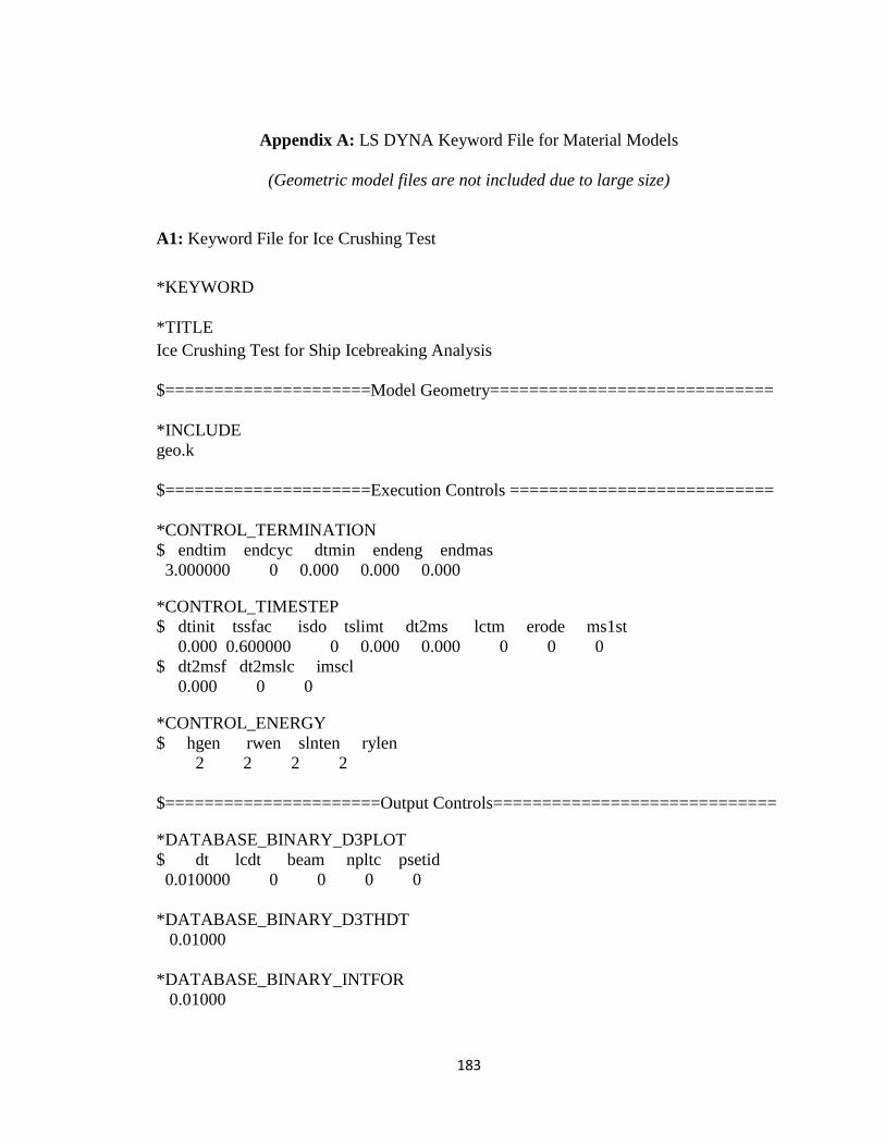
183

Appendix A: LS DYNA Keyword File for Material Models

(Geometric model files are not included due to large size)

A1: Keyword File for Ice Crushing Test

*KEYWORD

*TITLE

Ice Crushing Test for Ship Icebreaking Analysis

$=====================Model Geometry=============================

*INCLUDE

geo.k

$=====================Execution Controls ===========================

*CONTROL_TERMINATION

$ endtim endcyc dtmin endeng endmas

3.000000 0 0.000 0.000 0.000

*CONTROL_TIMESTEP

$ dtinit tssfac isdo tslimt dt2ms lctm erode ms1st

0.000 0.600000 0 0.000 0.000 0 0 0

$ dt2msf dt2mslc imscl

0.000 0 0

*CONTROL_ENERGY

$ hgen rwen slnten rylen

2 2 2 2

$======================Output Controls=============================

*DATABASE_BINARY_D3PLOT

$ dt lcdt beam npltc psetid

0.010000 0 0 0 0

*DATABASE_BINARY_D3THDT

0.01000

*DATABASE_BINARY_INTFOR

0.01000

184

*DATABASE_RCFORC

$ dt binary lcur ioopt

0.010000 0 0 0

*DATABASE_NODOUT

0.01000

*DATABASE_GLSTAT

0.01000

*DATABASE_MATSUM

0.01000

*DATABASE_EXTENT_BINARY

$ neiph neips maxint strflg sigflg epsflg rltflg engflg

0 0 3 1 0 0 0 0

$ cmpflg ieverp beamip dcomp shge stssz n3thdt ialemat

0 0 0 0 0 0 0 0

$ nintsld pkp_sen sclp unused msscl therm iniout iniout

0 0 0.000 0 0 0

$======================Part Id, Section Id, Mat Id======================

*PART

P1 - Indenter

$ pid secid mid eosid hgid grav adpopt tmid

1 1 1 0 0 0 0 0

P2 – Ice Wedge


2 2 2 0 0 0 0 0

*SECTION_SHELL

$ secid elform shrf nip propt qr/irid icomp setyp

1 2 0.8330 2.0 1.0 0.0 1

$ t1 t2 t3 t4 nloc marea

0.37 0.37 0.37 0.37 0.0

*SECTION_SOLID

$ secid elform aet

2 1 0

185

*MAT_RIGID

$ mid ro e pr n couple m alias

1 7850.000 2.000E+11 0.300000 0.000 0.000 0.000

$ cmo con1 con2

0.000 0 0

0.000 0.000 0.000 0.000 0.000 0.000

*MAT_PLASTIC_KINEMATIC

$ mid rho e pr sigy etan beta

2 900.0 5.00E9 0.300000 4.50E6 0.000 0.000

$ src srp fs vp

0.000 0.000 1.000E-4 0.000

$=========================Contacts===============================

*CONTACT_AUTOMATIC_NODES_TO_SURFACE

$ ssid msid sstyp mstyp sboxid mboxid spr mpr

1 2 3 3 0 0 1 1

$ fs fd dc vc vdc penchk bt dt

$ sfs sfm sst mst sfst sfmt fsf vsf

$================BC, IC, Body Loads and Force Field====================

*BOUNDARY_PRESCRIBED_MOTION_RIGID

$ pid dof vad lcid sf vid death birth

2 2 0 1 1.000000

*BOUNDARY_SPC_SET

$# nsid cid dofx dofy dofz dofrx dofry dofrz

1 0 1 0 1 1 1 1

*DEFINE_CURVE

$ lcid sidr sfa sfo offa offo dattyp

1

$ a1 o1

0.000 0.5000

100.00000 0.5000

$==============================================================

*END

186

A2: Keyword File for Four Point Bending Test

*KEYWORD

*TITLE

Four Point Bending Test for Ship Icebreaking Analysis

$=====================Model Geometry=============================

*INCLUDE

geo.k




10.000000 0 0.000 0.000 0.000

*CONTROL_TIMESTEP


0.000 0.600000 0 0.000 0.000 0 0 0


0.000 0 0

*CONTROL_ENERGY


2 2 2 2

$======================Output Controls=============================



0.010000 0 0 0 0


0.01000


0.01000

*DATABASE_RCFORC


0.010000 0 0 0

187

*DATABASE_NODOUT

0.01000

*DATABASE_GLSTAT

0.01000

*DATABASE_MATSUM

0.01000



0 0 3 1 0 0 0 0


0 0 0 0 0 0 0 0


0 0 0.000 0 0 0


*PART

P1 – Upper Support


1 1 1 0 0 0 0 0

P2 – Lower Support


2 1 1 0 0 0 0 0

P3 – Ice Beam


3 2 2 0 0 0 0 0

*SECTION_SHELL


1 2 0.8330 2.0 1.0 0.0 1


0.01 0.01 0.01 0.01 0.0

*SECTION_SOLID

$ secid elform aet

2 1 0

188

*MAT_RIGID


1 7850.000 2.000E+11 0.300000 0.000 0.000 0.000

$ cmo con1 con2

0.000 0 0

0.000 0.000 0.000 0.000 0.000 0.000

*MAT_PLASTICITY_COMPRESSION_TENSION

$ mid ro e pr c p fail tdel

2 900.000 5.0000E+9 0.300000 0.000 0.000 7.0000E-4 0.000

$ lcidc lcidt lcsrc lcsrt srflag lcfail ec rpct

1 2 3 0 0.000 0 0.000 0.000

$ pc pt pcutc pcutt pcutf

0.0 0.00 0.00 0.00 0.00

$ k

0.00

$=========================Contacts===============================



3 1 3 3 0 0 1 1





3 2 3 3 0 0 1 1






2 3 0 4 1.000000

*BOUNDARY_SPC_SET

$ nsid cid dofx dofy dofz dofrx dofry dofrz

1 0 1 1 1 1 1 1

*BOUNDARY_SPC_SET

189


2 0 1 1 0 1 1 1

*DEFINE_CURVE


1

$ a1 o1

0.000 5.8e6

1.00000 1.15e7

*DEFINE_CURVE


2

$ a1 o1

0.000 5.8e5

2.00000 1.258e7

*DEFINE_CURVE


3

$ a1 o1

10e-9 0.2700

10e-8 0.3360

10e-7 0.41700

10e-6 0.520

10e-5 0.643

10e-4 0.8000

10e-3 1.0000

10e-2 1.2200

10e-1 1.520

1.00 1.8900

10.0 2.348

100 2.91

1000 3.620

*DEFINE_CURVE


4

$ a1 o1

0.000 0.0010

100.00000 0.0010

$==============================================================

*END

190

A3: Keyword File for Water Foundation test

*KEYWORD

*TITLE

Water Foundation Test for Ship Icebreaking Analysis

$=====================Model Geometry=============================

*INCLUDE

geo.k




20.000000 0 0.000 0.000 0.000

*CONTROL_TIMESTEP


0.000 0.600000 0 0.000 0.000 0 0 0


0.000 0 0

*CONTROL_ENERGY


2 2 2 2

$======================Output Controls=============================



0.010000 0 0 0 0


0.01000


0.01000

*DATABASE_RCFORC


0.010000 0 0 0

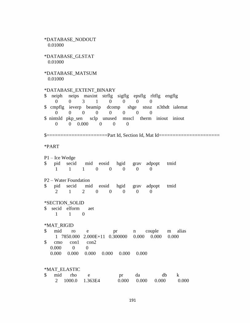
191

*DATABASE_NODOUT

0.01000

*DATABASE_GLSTAT

0.01000

*DATABASE_MATSUM

0.01000



0 0 3 1 0 0 0 0


0 0 0 0 0 0 0 0


0 0 0.000 0 0 0


*PART

P1 – Ice Wedge


1 1 1 0 0 0 0 0

P2 – Water Foundation


2 1 2 0 0 0 0 0

*SECTION_SOLID

$ secid elform aet

1 1 0

*MAT_RIGID


1 7850.000 2.000E+11 0.300000 0.000 0.000 0.000

$ cmo con1 con2

0.000 0 0

0.000 0.000 0.000 0.000 0.000 0.000

*MAT_ELASTIC

$ mid rho e pr da db k

2 1000.0 1.363E4 0.000 0.000 0.000 0.000

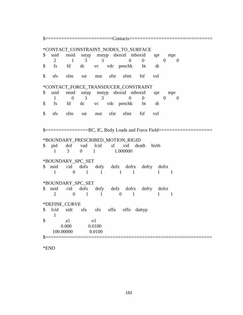
192

$=========================Contacts===============================

*CONTACT_CONSTRAINT_NODES_TO_SURFACE


2 1 3 3 0 0 0 0



*CONTACT_FORCE_TRANSDUCER_CONSTRAINT


1 0 3 3 0 0 0 0






1 3 0 1 1.000000

*BOUNDARY_SPC_SET


1 0 1 1 1 1 1 1

*BOUNDARY_SPC_SET


2 0 1 1 0 1 1 1

*DEFINE_CURVE


1

$ a1 o1

0.000 0.0100

100.00000 0.0100

$==============================================================

*END

193

Appendix B: LS DYNA Keyword File of Ship Ice Wedge Breaking

(Geometric model files are not included due to large size)

*KEYWORD

*TITLE

Simple Ship Ice Wedge Breaking Analysis

$=====================Model Geometry=============================

*INCLUDE

geo.k




10.000000 0 0.000 0.000 0.000

*CONTROL_TIMESTEP


0.000 0.600000 0 0.000 0.000 0 0 0


0.000 0 0

*CONTROL_ENERGY


2 2 2 2

$======================Output Controls=============================



0.010000 0 0 0 0


0.01000


0.01000

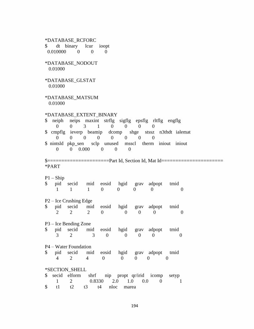
194

*DATABASE_RCFORC


0.010000 0 0 0

*DATABASE_NODOUT

0.01000

*DATABASE_GLSTAT

0.01000

*DATABASE_MATSUM

0.01000



0 0 3 1 0 0 0 0


0 0 0 0 0 0 0 0


0 0 0.000 0 0 0


*PART

P1 – Ship


1 1 1 0 0 0 0 0

P2 – Ice Crushing Edge


2 2 2 0 0 0 0 0

P3 – Ice Bending Zone


3 2 3 0 0 0 0 0

P4 – Water Foundation


4 2 4 0 0 0 0 0

*SECTION_SHELL


1 2 0.8330 2.0 1.0 0.0 0 1


195

0.37 0.37 0.37 0.37 0.0

*SECTION_SOLID

$ secid elform aet

2 1 0

*MAT_RIGID


1 7850.000 2.000E+11 0.300000 0.000 0.000 0.000

$ cmo con1 con2

0.000 0 0

0.000 0.000 0.000 0.000 0.000 0.000

*MAT_PLASTIC_KINEMATIC

$ mid rho e pr sigy etan beta

2 900.0 5.00E9 0.300000 4.50E6 0.000 0.000

$ src srp fs vp

0.000 0.000 1.000E-4 0.000

*MAT_PLASTICITY_COMPRESSION_TENSION

$ mid ro e pr c p fail tdel

3 900.000 5.0000E+9 0.300000 0.000 0.000 7.0000E-4 0.000

$ lcidc lcidt lcsrc lcsrt srflag lcfail ec rpct

1 2 3 0 0.000 0 0.000 0.000

$ pc pt pcutc pcutt pcutf

0.0 0.00 0.00 0.00 0.00

$ k

0.00

*MAT_ELASTIC

$ mid rho e pr da db k

4 1000.0 1.363E4 0.000 0.000 0.000 0.000

$=========================Contacts===============================



2 1 3 3 0 0 0 0





196

4 3 3 3 0 0 0 0





4 2 3 3 0 0 0 0






1 2 0 4 1.000000

*BOUNDARY_SPC_SET


1 0 1 1 1 1 1 1

*BOUNDARY_SPC_SET


2 0 1 0 1 1 1 1

*DEFINE_CURVE


1

$ a1 o1

0.000 5.8e6

1.00000 1.15e7

*DEFINE_CURVE


2

$ a1 o1

0.000 5.8e5

2.00000 1.258e7

*DEFINE_CURVE


3

$ a1 o1

197

10e-9 0.2700

10e-8 0.3360

10e-7 0.41700

10e-6 0.520

10e-5 0.643

10e-4 0.8000

10e-3 1.0000

10e-2 1.2200

10e-1 1.520

1.00 1.8900

10.0 2.348

100 2.91

1000 3.620

*DEFINE_CURVE


4

$ a1 o1

0.000 1.00

1.00000 1.00

$==============================================================

*END

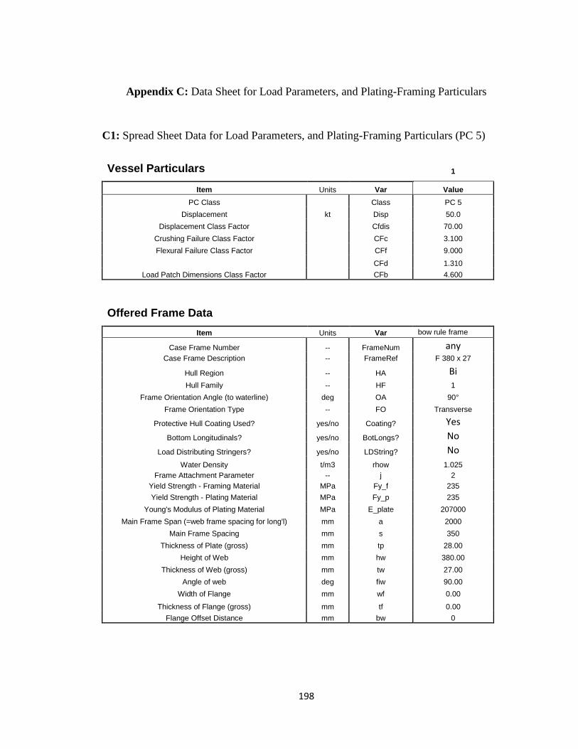
198

Appendix C: Data Sheet for Load Parameters, and Plating-Framing Particulars

C1: Spread Sheet Data for Load Parameters, and Plating-Framing Particulars (PC 5)

Vessel Particulars

1

Item Units Var Value

PC Class

Class PC 5

Displacement kt Disp 50.0

Displacement Class Factor

Cfdis 70.00

Crushing Failure Class Factor

CFc 3.100

Flexural Failure Class Factor

CFf 9.000

CFd 1.310

Load Patch Dimensions Class Factor CFb 4.600

Offered Frame Data

Item Units Var bow rule frame

Case Frame Number -- FrameNum any Case Frame Description -- FrameRef F 380 x 27

Hull Region -- HA Bi

Hull Family -- HF 1

Frame Orientation Angle (to waterline) deg OA 90°

Frame Orientation Type -- FO Transverse

Protective Hull Coating Used? yes/no Coating? Yes

Bottom Longitudinals? yes/no BotLongs? No

Load Distributing Stringers? yes/no LDString? No

Water Density t/m3 rhow 1.025

Frame Attachment Parameter -- j 2

Yield Strength - Framing Material MPa Fy_f 235

Yield Strength - Plating Material MPa Fy_p 235

Young's Modulus of Plating Material MPa E_plate 207000

Main Frame Span (=web frame spacing for long'l) mm a 2000

Main Frame Spacing mm s 350

Thickness of Plate (gross) mm tp 28.00

Height of Web mm hw 380.00

Thickness of Web (gross) mm tw 27.00

Angle of web deg fiw 90.00

Width of Flange mm wf 0.00

Thickness of Flange (gross) mm tf 0.00

Flange Offset Distance mm bw 0

199

Assesment Results for Offered Frames (net)

Web Buckling Constant -- wbc 215.8

Frame Stability Check (12.9.1) -- frstab OK

Web Thickness Min (12.9.3) -- webmin OK

Dist. to Plastc NA mm zna 8.5

Shell Plate Thickness - offered (net) mm tp 25.5

required value (12.4.2) (excl CA) mm t_reqd 25.1

OK

Frame Shear Area - offered (12.5.7) (net) cm2 Aw 98.8

required value (12.6.2 or ) cm2 At or AL 69.7

OK

Frame Modulus - offered (12.5.8) (net) cm3 Zp 1984.7

required value (12.6.3 or) cm3 Zpt or ZpL 1926.3

OK

Load Parameters

Force MN F 14.482

Aspect Ratio

AR 5.369

Line Load MN/m Q 3.723

Pressure MPa P 5.139

Ice Load Patch Width m w 3.890

Ice Load Patch Height m b 0.724

Average Patch Pressure MPa Pavg 5.139

Hull Area Factor

AF 1

Corrosion and Abrasion Allowance mm t_wear 2.5

Transverse Plating

Peak Pressure Factor - Plate (trans) - PPFpt 1.45

height of design load patch m bpt 0.724

Plate Thickness Required to Resist Ice Load mm t_net 25.1

Required Minimum Shell Plate Thickness mm t_min 27.599

Transverse Framing

Peak Pressure Factor - Transverse Frame - PPFt 1.45

Length of Loaded Portion of Span m LL 0.724

Required Shear Area of Transverse Frame cm2 At 69.7

Ratio of Minimum Shear Area / Fitted Shear Area a_1 0.705

Load Length Parameter - Y 0.819

Shear Parameter - kw 1.000

Width of Plating Acting Effectively With Frame mm beff 175

Sum of Plastic Moduli of Flange and Plate cm3 z_p 34.3

Shear Parameter - kz 0.0173

Interaction Eq For 3H Mechanism (Sym Load) - A1A 0.585

Interaction Eq For Shear Mechanism (Asym Load) - A1B 0.374

Interaction parameter - A1_ 0.585

Required Plastic Section Modulus of Transverse Frame cm3 Zpt 1926.3

200

Longitudinal Plating (b>=s)

Peak Pressure Factor - Plate (longl) - PPFpl 1.78



Longitudinal Plating (b<s)

Plate Thickness Required to Resist Ice Load mm t_net #NUM!

Required Minimum Shell Plate Thickness mm t_min #NUM!

Longitudinal Framing

Peak Pressure Factor - Transverse Frame - PPFs 1

Length of Loaded Portion of Span m b_1 0.299

load height parameter - ko 0.855

load height parameter m b_2 0.350

load height parameter - bpri 2.070

Required Shear Area of Longitudinal Frame cm2 AL 113.4


Shear Parameter - kwl 1.000

Interaction Eq For 3H Mechanism (Sym Load) - A4_ 1.000

Required Plastic Section Modulus of Longitudinal Frame cm3 ZpL 3272275.4

Required Plating

ratio angFac 0.00

Plate Thickness Required to Resist Ice Load mm t_reqd 25.1


Required Framing

Required Shear Area of Between Frame cm2 A_reqd 69.7

Required Plastic Section Modulus of Longitudinal Frame cm3 Z_reqd 1926.3

Required Web Frames

Required Shear Area of Between Frame mm2 A_reqd 28830.1 Required Plastic Section Modulus of Longitudinal

Frame mm3 Z_reqd 10,350,646

201


Vessel Particulars

1


PC Class

Class PC 6



Cfdis 40.00


CFc 2.400


CFf 5.490

CFd 1.170


Offered Frame Data Item Units Var bow rule frame

Case Frame Number -- FrameNum any Case Frame Description -- FrameRef F 320 x 24


Hull Family -- HF 1



























202

OK



OK



OK

Load Parameters Force MN F 9.372

Aspect Ratio

AR 5.369






Hull Area Factor

AF 1

Corrosion and Abrasion Allowance mm t_wear 2

Transverse Plating Peak Pressure Factor - Plate (trans) - PPFpt 1.45




Transverse Framing Peak Pressure Factor - Transverse Frame - PPFt 1.45

















Longitudinal Plating (b<s)



203

Longitudinal Framing

Peak Pressure Factor - Transverse Frame - PPFs 1










Required Plating ratio angFac 0.00



Required Framing Required Shear Area of Between Frame cm2 A_reqd 47.8


Required Web Frames Required Shear Area of Between Frame mm2 A_reqd 19759.0

Required Plastic Section Modulus of Longitudinal Frame mm3 Z_reqd

7,093,915

204


Vessel Particulars


PC Class

Class PC 7



Cfdis 22.00


CFc 1.800


CFf 4.060

CFd 1.110


Offered Frame Data Item Units Var bow rule frame

Case Frame Number -- FrameNum any Case Frame Description -- FrameRef HP 320*16.0


Hull Family -- HF 1



























205

OK



OK



OK

Load Parameters Force MN F 6.871

Aspect Ratio

AR 5.369






Hull Area Factor

AF 1

Corrosion and Abrasion Allowance mm t_wear 2

Transverse Plating Peak Pressure Factor - Plate (trans) - PPFpt 1.45




Transverse Framing Peak Pressure Factor - Transverse Frame - PPFt 1.45

















Longitudinal Plating (b<s) Plate Thickness Required to Resist Ice Load mm t_net 14.3


Longitudinal Framing Peak Pressure Factor - Transverse Frame - PPFs 1

206










Required Plating ratio angFac 0.00



Required Framing Required Shear Area of Between Frame cm2 A_reqd 37.7


Required Web Frames Required Shear Area of Between Frame mm2 A_reqd 15588.4

Required Plastic Section Modulus of Longitudinal Frame mm3 Z_reqd

5,596,592