µ-diff: an open-source Matlab toolbox for computing multiple

scattering problems by disks

Bertrand Thierry∗, Xavier Antoine†, Chokri Chniti‡ and Hasan Alzubaidi‡

Abstract

The aim of this paper is to describe a Matlab toolbox, called µ-diff, for modeling andnumerically solving two-dimensional complex multiple scattering by a large collection of circularcylinders. The approximation methods in µ-diff are based on the Fourier series expansions ofthe four basic integral operators arising in scattering theory. Based on these expressions, anefficient spectrally accurate finite-dimensional solution of multiple scattering problems can besimply obtained for complex media even when many scatterers are considered as well as largefrequencies. The solution of the global linear system to solve can use either direct solvers orpreconditioned iterative Krylov subspace solvers for block Toeplitz matrices. Based on thisapproach, this paper explains how the code is built and organized. Some complete numericalexamples of applications (direct and inverse scattering) are provided to show that µ-diff is aflexible, efficient and robust toolbox for solving some complex multiple scattering problems.

Keywords: Multiple scattering, wave propagation, acoustics, electromagnetism, optics, computa-tional methods, numerical simulation, spectral method

MSC: 35J05, 78A45, 78A48, 76Q05, 65M70, 31A10

Contents

1 Program Summary 2

2 Introduction 3

3 Basic theory behind µ-diff: integral equations and formulations for 2D scatteringproblems 43.1 Definitions and basics on integral operators for scattering . . . . . . . . . . . . . . . 43.2 A few boundary integral equations for the Dirichlet problem . . . . . . . . . . . . . . 6

∗Laboratoire J.L. Lions (LJLL), University of Paris VI, Paris, France. (bthierry@math.cnrs.fr).†Universite de Lorraine, Institut Elie Cartan de Lorraine, UMR 7502, Vandoeuvre-les-Nancy, F-54506, France.

(xavier.antoine@univ-lorraine.fr).‡Department of Mathematics, University College in Qunfudah, Umm Al-Qura University, Saudi Arabia.

(cachniti@uqu.edu.sa;hmzubaidi@uqu.edu.sa).

1

arX

iv:1

409.

8186

v1 [

cs.M

S] 2

9 Se

p 20

14

4 Spectral formulation used in µ-diff 74.1 Notations and Fourier basis . . . . . . . . . . . . . . . . . . . . . . . . . . . . . . . . 84.2 Integral operators - integral equations for a cluster of circular cylinders . . . . . . . . 94.3 Projection of the incident waves in the Fourier basis . . . . . . . . . . . . . . . . . . 114.4 Near- and far-fields evaluations . . . . . . . . . . . . . . . . . . . . . . . . . . . . . . 12

5 Finite-dimensional approximations and numerical solutions proposed in µ-diff 13

6 Structure of the µ-diff Matlab toolbox 146.1 Pre-processing: physical and geometrical configurations . . . . . . . . . . . . . . . . 156.2 Defining and solving an integral equation . . . . . . . . . . . . . . . . . . . . . . . . 166.3 Post-processing of computed outputs . . . . . . . . . . . . . . . . . . . . . . . . . . . 17

7 Numerical examples with µ-diff 177.1 Example I: scattering by randomly distributed sound-soft or sound-hard circular

cylinders . . . . . . . . . . . . . . . . . . . . . . . . . . . . . . . . . . . . . . . . . . . 177.2 Example II: multiple scattering by a cluster of homogeneous penetrable obstacles . . 187.3 Example III: a more advanced application in time reversal . . . . . . . . . . . . . . . 20

8 Conclusion 22

1 Program Summary

Manuscript title: µ-diff: an open Matlab toolbox for computing multiple scattering problems by disksAuthors: Xavier ANTOINE & Bertrand THIERRYProgram title: µ-diffLicensing provisions: Standard CPC licenceProgramming language: MatlabComputer(s) for which the program has been designed: PC, MacOperating system(s) for which the program has been designed: Windows, Mac OS, LinuxRAM required to execute with typical data: 2000 MegabytesHas the code been vectorised or parallelized?: YesNumber of processors used: Most if not allKeywords: Matlab, Multiple scattering, waves, random media, acoustics, optics, electromagnetism,numerical methodsCPC Library Classification: 4.6, 10, 18Nature of problem: Modeling and simulation of two-dimensional multiple wave scattering by largeclusters of circular cylinders for any frequency. The program is well-designed to manage highlyaccurate solutions for deterministic or random media, with various boundary conditions and physicsproperties of the scatterers. Pre- and post-processing facilities are designed specifically for theseproblems.Solution method: We use spectral Fourier approximation schemes and direct or iterative Krylovsubspace methods.Running time: From a few seconds for simple problems to a few minutes for more complex situationson a medium computer.

2

2 Introduction

Let us consider M regular, bounded and disjoint scatterers Ω−p , p = 1, ...,M , distributed in R2,with boundary Γp := Ω−p . The scatterer Ω− is defined as the collection of the M separate obstacles,

i.e. Ω− = ∪Mp=1Ω−p , with boundary Γ = ∪Mp=1Γp. The homogeneous and isotropic exterior domain of

propagation is Ω+ = R2 \Ω−. For the sake of conciseness in the presentation, we first assume thatthe scatterers are sound-soft (Dirichlet boundary condition), but other situations can be handled bythe µ-diff (multiple-diffraction) Matlab toolbox (e.g. sound-hard scatterers, impedance boundaryconditions, penetrable scatterers) as it will be shown during the numerical examples (see section 7).We now consider a time-harmonic incident acoustic plane wave uinc(x) = eikβ·x (with x = (x1, x2) ∈R2) illuminating Ω−, with an incidence direction β = (cos(β), sin(β)) and a time dependence e−iωt,where ω is the wave pulsation and k is the wavenumber. The sound-soft multiple scattering problemof uinc by Ω− consists in computing the scattered wavefield u as the solution to the boundary-valueproblem [7, 37]

(∆ + k2)u = 0, in Ω+,u = −uinc, on Γ,

lim||x||→+∞

||x||1/2(∇u · x

||x||− iku

)= 0.

(1)

The operator ∆ = ∂2x1 + ∂2

x2 is the Laplace operator and (∆ + k2) is the Helmholtz operator. Thegradient operator is ∇ and ||x|| =

√x · x, where x · y is the scalar product of two vectors x and y

of R2. The last equation of (1) is the well-known Sommerfeld’s radiation condition at infinity thatensures the uniqueness of u [18, 41].

Multiple scattering is known to be a very complicated and challenging problem in terms ofcomputational method [1, 2, 3, 7, 8, 16, 22, 23, 28, 30, 36, 51] since the incident wave is multiplydiffracted by all the single scatterers involved in the geometrical configuration. As a consequence,the scattered wavefield has a highly complicated structure and exhibits some particular physicsproperties. The toolbox µ-diff1 contributes to the development of reliable and efficient numericalmethods to understand and simulate such problems. It uses the powerful and mathematicallyrigorous integral equation formulation methods for solving multiple scattering problems. Beingable to use integral operators allows us to formulate the solution to a given scattering problemby using traces theorems and variational approaches (see section 3). When the boundary Γ isgeneral, then boundary element discretization techniques are required [6, 7, 18, 37, 41]. Even ifthese methods are extremely useful for general shapes, they also have some disadvantages. First,they lead to solving large full linear systems, most particularly when investigating small wavelengthproblems (λ 1) and large scatterers (size(Ω−) 1) or collections of many scatterers (M 1).These systems require a lot of memory storage and their solution is highly time consuming. Thesolution can be accelerated by using Krylov subspace solvers [4, 5, 6, 44] in conjunction with fastmatrix-vector products algorithms (for example Multilevel Fast Multipole Methods [29] or othercompression techniques [7, 28]) but at the price of a loss of accuracy/stability. Second, even ifboundary element methods provide an accurate solution, the precision is limited since linear finiteelement spaces are used as well as low-order surface descriptions. Going to higher order basisfunctions is very complicated and time consuming, most particularly when one wants to integratewith high accuracy (hyper)singular potentials that are involved in an integral formulation.

1http://mu-diff.math.cnrs.fr

3

When the geometry is more trivial, then further simplifications can be realized in the integralequation methods. Indeed, for example, analytical expressions of the integral operators can beobtained, and spectrally accurate and fast solutions can be derived. This is the case when consid-ering a disk [7, 37]. The Matlab toolbox µ-diff considers the case of a collection of M homogeneouscircular cylinders where Fourier basis expansions can be used (see section 4). Even if disks can beconsidered as simple geometries, a reliable and highly accurate solution is required for wave propa-gation problems (acoustics, electromagnetics, optics, nanophotonics, elasticity) that involve manycircular scatterers, modeling structured or disordered media, most particularly when k and M arelarge (see e.g. [9, 15, 19, 20, 21, 22, 24, 33, 34, 35, 36, 39, 40, 42, 45, 49, 50, 52]). Let us note thatall the developments in this paper directly apply to 2D TM/TE electromagnetic scattering waves[37] even if our presentation is more related to acoustics. Furthermore, since multiple scattering is ahighly complex problem with unusual properties, it is desirable to have a simple modeling tool thathelps to understand the physics properties of such structures. Finally, having a reference solutionmethod for multiple scattering leads to the possibility of evaluating the accuracy and performanceof other more general numerical methods like finite element or general integral equation solvers.The goal of the µ-diff Matlab toolbox is to contribute to these different questions.

The structure of the paper is the following. In section 3, we describe the basics of integraloperators that are used in µ-diff and review the most standard integral equation formulations whenone wants to solve the sound-soft scattering problem. In Section 4, we explain the approximationmethod that is used in µ-diff to solve the integral equation problems through Fourier series expan-sions and how to formulate post-processing data (near- and far-fields for example). In section 5, wedescribe the finite-dimensional approximation leading to concrete linear systems. Some numericalaspects of the resolution methods are also discussed. Section 6 details the structure of the µ-diffcode and the main functions that are included. To illustrate the use of µ-diff, we provide in sections7.1 and 7.2 some numerical examples for direct multiple scattering problems (sound-soft, sound-hard, penetrable scatterers). In addition, we consider in section 7.3 a more advanced examplerelated to the DORT method (Time Reversal method) in the presence of homogeneous penetrablecircular scatterers. All the related files are available in the µ-diff package when downloaded andthe simulations can be reproduced. Finally, we conclude in section 8.

3 Basic theory behind µ-diff: integral equations and formulationsfor 2D scattering problems

3.1 Definitions and basics on integral operators for scattering

Let G be the two-dimensional free-space Green’s function defined by

∀x,y ∈ R2,x 6= y, G(x,y) =i

4H

(1)0 (k‖x− y‖).

The function H(1)0 is the first-kind Hankel function of order zero. Integral equations are essentially

based upon the Helmholtz integral representation formula [18, Theorems 3.1 and 3.3].

Proposition 1. If v is a solution to the Helmholtz equation in an unbounded connected domain

4

Ω+ and satisfies the Sommerfeld radiation condition, then we have∫Γ−G(x,y)∂nv(y) + ∂nyG(x,y)v(y) dΓ(y) =

v(x) if x ∈ Ω+,

0 otherwise.(2)

If v− is solution to the Helmholtz equation in a bounded domain Ω−, then one gets∫Γ−G(x,y)∂nv

−(y) + ∂nyG(x,y)v−(y) dΓ(y) =

0 if x ∈ Ω+,

−v−(x) otherwise.(3)

The integrals on Γ must be understood as duality brackets between the Sobolev space H1/2(Γ)and its dual space H−1/2(Γ). Nevertheless, when the incident wavefield uinc and the curve Γ aresufficiently smooth, the scattered field is then regular and the duality bracket can be identified (thisis systematically the case in the presentation) to the (non hermitian) inner product in L2(Γ)

〈f, g〉H−1/2,H1/2 =

∫ΓfgdΓ.

Let us now introduce the volume single- and double-layer integral operators, respectively de-noted by L and M , and defined by: ∀x ∈ R2\Γ

L : ρ 7−→ L ρ(x) =

∫ΓG(x,y)ρ(y) dΓ(y),

M : λ 7−→ Mλ(x) = −∫

Γ∂nyG(x,y)λ(y) dΓ(y).

We can then express the wavefields v and v− (see equations 2 and 3) asv(x) = −L (∂nv|Γ)(x)−M (v|Γ)(x), ∀x ∈ Ω+,

v−(x) = L (∂nv−|Γ)(x) + M (v−|Γ)(x), ∀x ∈ Ω−.

Furthermore, the single- and double-layer integral operators provide some outgoing solutions to theHelmholtz equation [17].

Proposition 2. For any densities ρ ∈ H−1/2(Γ) and λ ∈ H1/2(Γ), the functions L ρ and Mλ aresome outgoing solutions to the Helmholtz equation in R2\Γ.

We now recall the expressions of the trace and normal derivative trace of the volume single-and double-layer potentials which are commonly called jump relations [17, Theorem 3.1].

Proposition 3. For any x in Γ, the trace and normal derivative traces of the operators L and Mare given by the following relations (the signs indicate that z tends towards x from the exterior orthe interior of Γ)

limz∈Ω±→x

L ρ(z) = Lρ(x), limz∈Ω±→x

Mλ(z) =

(∓1

2I +M

)λ(x),

limz∈Ω±→x

∂nzL ρ(z) =

(∓1

2I +N

)ρ(x), lim

z∈Ω±→x∂nzMλ(z) = Dλ(x),

(4)

5

where I is the identity operator, for x ∈ Γ,

Lρ(x) =

∫ΓG(x,y)ρ(y)dΓ(y), Mλ(x) = −

∫Γ∂nyG(x,y)λ(y)dΓ(y),

Nρ(x) =

∫Γ∂nxG(x,y)ρ(y)dΓ(y) = −M∗ρ(x), Dλ(x) = −∂nx

∫Γ∂nyG(x,y)λ(y)dΓ(y).

Throughout the paper, the boundary integral operators are denoted by a roman letter (e.g. L)while the volume integral operators use a calligraphic letter (e.g. L ). The operator M∗ = −N isthe adjoint operator of M , that is

〈g,Mf〉H−1/2,H1/2 = 〈−Ng, f〉H−1/2,H1/2 , ∀(f, g) ∈ H1/2(Γ)×H−1/2(Γ).

Other properties like compactness or invertibility of integral operators can also be stated [7, 18, 41].

3.2 A few boundary integral equations for the Dirichlet problem

The aim of this section is to provide without details the most standard integral equation formu-lations for solving the 2D scattering problem with Dirichlet boundary condition. These equationsserve as model examples for explaining the way µ-diff works in sections 6 and 7. We refer to[6, 46, 47] for further explanations concerning the derivation and properties of these integral equa-tions (like for the well-posedness and the possible existence of resonant modes).

The first three integral equations presented here are based on a single-layer representation only

u = L ρ.

From this representation and by using the jump relations, it can be proved that the density ρ isequal to (−∂nu − ∂nuinc)|Γ and thus has a physical meaning. The first integral equation, whichis usually called Electric Field Integral Equation (EFIE), is based on the trace of the single-layeroperator

Lρ = −uinc|Γ. (5)

The equation is well-posed and equivalent to the exterior scattering problem (1) as soon as k is notan irregular interior frequency of the associated Dirichlet boundary-value problem [6, 46].

A second equation, designated by Magnetic Field Integral Equation (MFIE), is(1

2I +N

)ρ = −∂nuinc|Γ.

It is also well-posed and equivalent to the exterior scattering problem (1) if k is not an interiorNeumann resonance [6, 46].

To avoid the interior resonance problem, Burton and Miller [6, 14, 46] consider a linear combi-nation of the EFIE and MFIE. Let α be a real-valued parameter such that: 0 < α < 1, and η bea complex number which satisfies =(η) 6= 0, where =(η) is the imaginary part of η (the real part is<(η)). Then, the Combined Field Integral Equation (CFIE) [6, 31, 46] (also called Burton-Millerintegral equation) is given by[

(1− α)

(1

2I +N

)+ αηL

]ρ = −

[(1− α)∂nu

inc|Γ + αηuinc|Γ].

6

This integral equation is well-posed for any wavenumber k.Let us now consider η as a complex-valued parameter with non zero imaginary part. Then,

a fourth integral representation is based on a linear combination of the single- and double-layerpotentials

utot = −(ηL + M )ψ + uinc,

where the total wavefield is defined by utot := u+ uinc. The resulting integral equation is obtainedby taking the trace of the above relation (see equations (4))[

−ηL−M +1

2I

]ψ = −uinc|Γ. (6)

This equation, called Brakhage-Werner Integral Equation (BWIE) [12], is well-posed for any k andis equivalent to the exterior scattering problem. Finally, let us note that the surface density ψ isunphysical unlike for the three previous equations.

When Ω− =⋃Mp=1 Ωp is multiply connected, all the integral operators can be written by blocks.

For example, the single-layer potential L ρ can be expressed as the sum of elementary potentials

L ρ =

M∑p=1

Lpρp,

where ρp = ρ|Γp and

Lpρp(x) =

∫Γp

G(x,y)ρp(y) dx, ∀x ∈ R2\Ωp.

Another way of writing the EFIE (5) is thenL1,1 L1,2 . . . L1,M

L2,1 L2,2 . . . L2,M...

.... . .

...LM,1 LM,2 . . . LM,M

ρ1

ρ2...ρM

= −

uinc|Γ1

uinc|Γ2

...uinc|ΓM

,

where Lp,qρq = (Lqρq)|Γp , with

∀x ∈ Γ, Lqρq(x) =

∫Γq

G(x,y)ρq(x) dy.

4 Spectral formulation used in µ-diff

We consider now circular cylinders as scatterers. In this situation, we can explicitly computethe boundary integral equations in a Fourier basis, leading therefore to an efficient computationalspectral method when used in conjunction with numerical linear algebra methods (direct or iterativesolvers).

7

x

bpqOp

Oq

bq

bp

Ω−p

Ω−q

O x1

x2

rp(x)

rq(x)

αpq

r(x)

αqθ(x)

αp

θq(x)

θp(x)

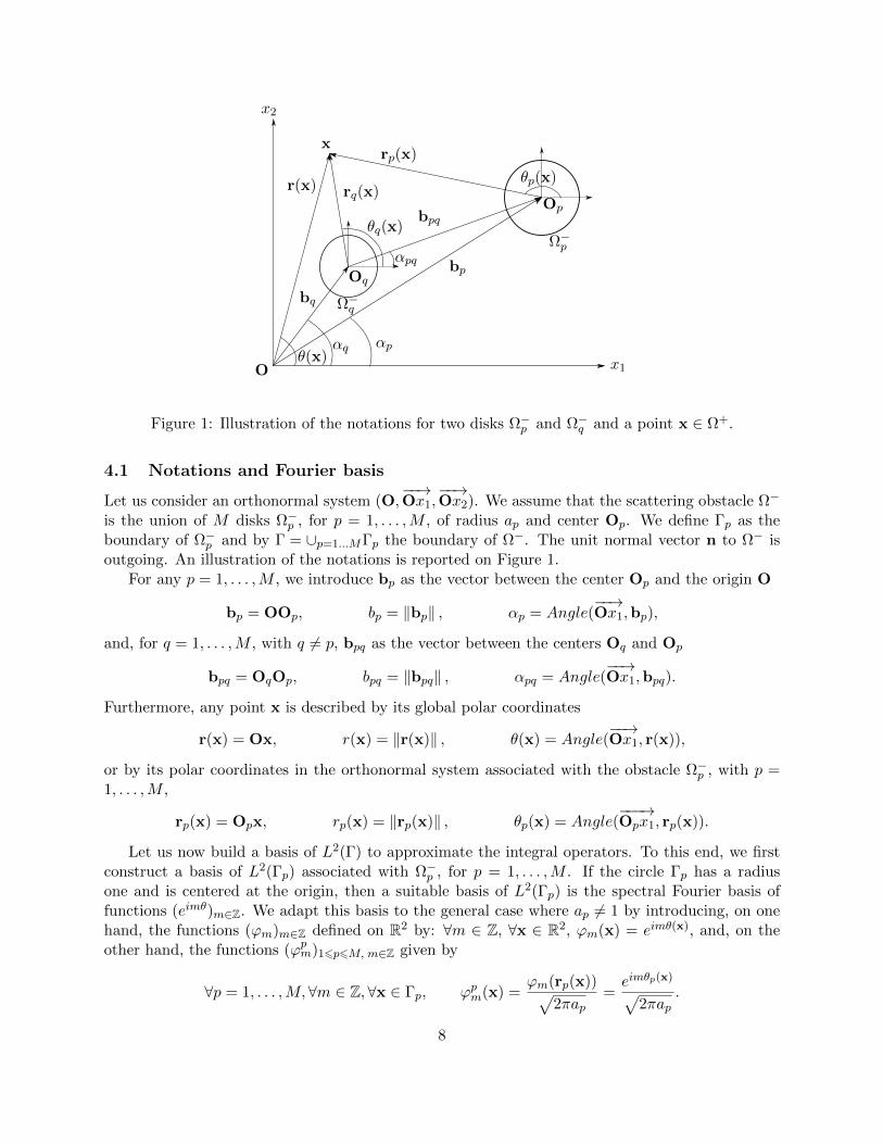
Figure 1: Illustration of the notations for two disks Ω−p and Ω−q and a point x ∈ Ω+.

4.1 Notations and Fourier basis

Let us consider an orthonormal system (O,−−→Ox1,

−−→Ox2). We assume that the scattering obstacle Ω−

is the union of M disks Ω−p , for p = 1, . . . ,M , of radius ap and center Op. We define Γp as theboundary of Ω−p and by Γ = ∪p=1...MΓp the boundary of Ω−. The unit normal vector n to Ω− isoutgoing. An illustration of the notations is reported on Figure 1.

For any p = 1, . . . ,M , we introduce bp as the vector between the center Op and the origin O

bp = OOp, bp = ‖bp‖ , αp = Angle(−−→Ox1,bp),

and, for q = 1, . . . ,M , with q 6= p, bpq as the vector between the centers Oq and Op

bpq = OqOp, bpq = ‖bpq‖ , αpq = Angle(−−→Ox1,bpq).

Furthermore, any point x is described by its global polar coordinates

r(x) = Ox, r(x) = ‖r(x)‖ , θ(x) = Angle(−−→Ox1, r(x)),

or by its polar coordinates in the orthonormal system associated with the obstacle Ω−p , with p =1, . . . ,M ,

rp(x) = Opx, rp(x) = ‖rp(x)‖ , θp(x) = Angle(−−−→Opx1, rp(x)).

Let us now build a basis of L2(Γ) to approximate the integral operators. To this end, we firstconstruct a basis of L2(Γp) associated with Ω−p , for p = 1, . . . ,M . If the circle Γp has a radiusone and is centered at the origin, then a suitable basis of L2(Γp) is the spectral Fourier basis offunctions (eimθ)m∈Z. We adapt this basis to the general case where ap 6= 1 by introducing, on onehand, the functions (ϕm)m∈Z defined on R2 by: ∀m ∈ Z, ∀x ∈ R2, ϕm(x) = eimθ(x), and, on theother hand, the functions (ϕpm)16p6M, m∈Z given by

∀p = 1, . . . ,M,∀m ∈ Z, ∀x ∈ Γp, ϕpm(x) =ϕm(rp(x))√

2πap=eimθp(x)√

2πap.

8

For p = 1, . . . ,M , the family (ϕpm)m∈Z forms an orthonormal basis of L2(Γp) for the hermitianinner product (·, ·)L2(Γp)

∀f, g ∈ L2(Γp), (f, g)L2(Γp) =

∫Γp

f(x)g(x)dΓp(x).

To build a basis of L2(Γ), we introduce the functions Φpm of L2(Γ) as the union of these M families

∀p, q = 1, . . . ,M,∀m ∈ Z, Φpm|Γq =

0 if q 6= p,

ϕpm if q = p.

The family B = Φpm, m ∈ Z, p = 1, . . . ,M, also called Fourier or spectral basis, is a Hilbert basis

of L2(Γ) for the usual scalar product (·, ·)L2(Γ).

4.2 Integral operators - integral equations for a cluster of circular cylinders

In view of a numerical procedure, µ-diff uses the weak formulation of the EFIE (5) in L2(Γ) basedon the Fourier basis B

Find ρ ∈ H−1/2(Γ) such that for any p = 1, . . . ,M, and m ∈ Z,

(Lρ,Φpm)L2(Γ) = −

(uinc|Γ,Φp

m

)L2(Γ)

.

Since uinc is assumed to be smooth enough (typically C∞) and that Γ is C∞, then the scatteredwavefield is also C∞(Ω+) and the density ρ is (at least) in H1/2(Γ). Therefore, ρ can be expandedin B as

ρ =M∑q=1

∑n∈Z

ρqnΦqn

and the weak form of the EFIE isFind the Fourier coefficients ρqn ∈ C, for q = 1, . . . ,M , and n ∈ Z, such that,

∀p = 1, . . . ,M, ∀m ∈ Z,M∑q=1

∑n∈Z

ρqn (LΦqn,Φ

pm)L2(Γ) = −

(uinc|Γ,Φp

m

)L2(Γ)

.

This formulation can be written under the following matrix form Lρ = U, where the infinite matrixrepresentation L = (Lp,q)16p,q6M and the infinite vectors ρ = (ρp)16p6M and U = (Up)16p6M aredefined by blocks as

L =

L1,1 L1,2 . . . L1,M

L2,1 L2,2 . . . L2,M

......

. . ....

LM,1 LM,2 . . . LM,M

, ρ =

ρ1

ρ2

...

ρM

, U =

U1

U2

...

UM

, (7)

with, for any p, q = 1, . . . ,M , and m,n ∈ Z: Lp,qm,n = (LΦqn,Φ

pm)L2(Γ), ρpm = ρpm and Up

m =(−uinc|Γ,Φp

m

)L2(Γ)

.

9

For the other integral formulations (section 3.2) or even for any other boundary condition, theexpressions of the three boundary integral operatorsM , N andD are needed. Therefore, to computean integral equation, we introduce the infinite matrices M = (Mp,q)16p,q6M , N = (Np,q)16p,q6M and

D = (Dp,q)16p,q6M , with the same block structure as L (see equation (7)). For p, q = 1, . . . ,M , the

coefficients of the infinite matrices Mp,q, Np,q and Dp,q are defined for any indices m and n in Z by

Mp,qm,n = (MΦq

n,Φpm)L2(Γ) , N

p,qm,n = (NΦq

n,Φpm)L2(Γ) , and Dp,qm,n = (DΦq

n,Φpm)L2(Γ) .

For a numerical implementation, we can explicitly compute [8, 46] the matrix blocks Lp,q, Mp,q,Np,q and Dp,q involved in L, M, N and D, for p, q = 1, . . . ,M . To this end, we introduce the infinitediagonal matrices Jp, (dJ)p, Hp and (dH)p, with general terms, for m ∈ Z,

Jpmm = Jm(kap), (dJ)pmm = J ′m(kap), Hpmm = H(1)

m (kap), (dH)pmm = H(1)′m (kap).

In addition, let Ip be the infinite identity matrix, and, for q 6= p, the infinite separation matrix Sp,qbetween the obstacles Ω−p and Ω−q , defined by

Sp,q = (Sp,qm,n)m∈Z,n∈Z and Sp,qm,n = Smn(bpq) = H(1)m−n(kbpq)e

i(m−n)αbq .

Under these notations, we rewrite the blocks Lp,q, Mp,q, Np,q and Dp,q of the infinite matrices L,M, N and D under the matrix form, for any p, q = 1, . . . ,M ,

• Lp,q =

iπap

2JpHp, if p = q,

iπ√apaq

2Jp(Sp,q)T Jq, if p 6= q,

• Mp,q =

−1

2Ip − iπkap

2Jp(dH)p =

1

2Ip − iπkap

2(dJ)pHp, if p = q,

−ikπ√apaq

2Jp(Sp,q)T (dJ)q, if p 6= q,

• Np,q =

1

2Ip +

iπkap2

Jp(dH)p = −1

2Ip +

iπkap2

(dJ)pHp, if p = q,

ikπ√apaq

2(dJ)p(Sp,q)T Jq, if p 6= q,

• Dp,q =

iπk2ap

2(dJ)p(dH)p, if p = q,

−ik2π√apaq

2(dJ)p(Sp,q)T (dJ)q, if p 6= q,

where (Sp,q)T is the transpose matrix of the separation matrix Sp,q.The integral equations involve the trace or normal derivative trace of the incident wavefield on

Γ. We have already introduced the infinite vector U of the coefficients of uinc|Γ in the Fourier basis.We then define similarly the infinite vector dU = (dUp)16p6M of the coefficients of the normalderivative trace ∂nu

inc|Γ, such that

∀p = 1, . . . ,M, ∀m ∈ Z, (dU)pm =(∂nu

inc|Γ,Φpm

)L2(Γ)

.

10

Finally, the density changes according to the integral equation and most particularly with respectto the boundary condition. To keep the same notations as previously, we introduce the densities λand ψ (used in the BWIE) that are expanded in the Fourier basis as

λ =M∑p=1

∑m∈Z

λpmΦpm and ψ =

M∑p=1

∑m∈Z

ψpmΦpm.

Finally, we set: λ = (λp)16p6M and Ψ = (Ψp)16p6M , where each block λ

p= (λ

p

m)m∈Z and

Ψp = (Ψpm)m∈Z is defined by: ∀m ∈ Z, λ

p

m = λpm and Ψpm = ψpm.

4.3 Projection of the incident waves in the Fourier basis

To fully solve one of the integral equations (EFIE, MFIE, CFIE or Brakhage-Werner), we need tocompute the Fourier coefficients of the trace and normal derivative traces of the incident wave. Wegive the results for both an incident plane wave and a pointwise source term (Green’s function).

For an incident plane wave, the following proposition holds [3].

Proposition 4. Let us assume that uinc is an incident plane wave of direction β, with β =(cos(β), sin(β)) and β ∈ [0, 2π], i.e.

∀x ∈ R2, uinc(x) = eikβ·x.

Then we have the following equalities

Upm =

(uinc|Γ,Φp

m

)L2(Γ)

= dpmJm(kap), (dU)pm =(∂nu

inc|Γ,Φpm

)L2(Γ)

= kdpmJ′m(kap),

with dpm =√

2πapeikβ·bpeim(π/2−β).

Let us consider now an incident wave emitted by a pointwise source located at s ∈ Ω+, i.e. thewave uinc is the Green’s function centered at s. The Fourier coefficients of the trace and normalderivative trace of uinc on Γ are then given by the following proposition [46].

Proposition 5. Let s ∈ Ω+. We assume that the incident wave uinc is the Green’s functioncentered at s

∀x ∈ R2 \ s, uinc(x) = G(x, s) =i

4H

(1)0 (k‖x− s‖).

The Fourier coefficients in B of the trace and normal derivative trace of the incident wave on Γare respectively given by

Upm =

(uinc|Γ,Φp

m

)L2(Γ)

=iπap

2Jm(kap)H

(1)m (krp(s))Φp

m(s)

and

(dU)pm =(∂nu

inc|Γ,Φpm

)L2(Γ)

= kiπap

2J ′m(kap)H

(1)m (krp(s))Φp

m(s).

11

4.4 Near- and far-fields evaluations

By using the Graf’s addition theorem [37, 46], we can compute the expression of the single- anddouble-layer potentials at a point x located in the propagation domain Ω+.

Proposition 6. Let ρ ∈ L2(Γ) and µ ∈ H1/2(Γ) be two densities admitting the following decompo-sitions in the Fourier basis B

ρ =M∑p=1

∑m∈Z

ρpmΦpm and λ =

M∑p=1

∑m∈Z

λpmΦpm.

Then, for any point x in the domain of propagation Ω+, the single-layer potential reads

L ρ(x) =

M∑p=1

∑m∈Z

ρpmL Φpm(x) =

M∑p=1

∑m∈Z

ρpmiπap

2Jm(kap)H

(1)m (krp(x))Φp

m(x),

and the double-layer potential can be expressed as

Mλ(x) =

M∑p=1

∑m∈Z

λpmM Φpm(x) = −

M∑p=1

∑m∈Z

λpmiπkap

2J ′m(kap)H

(1)m (krp(x))Φp

m(x).

Proposition 6 implies that, for any x in Ω+,

u(x) = L ρ(x) + Mλ(x) =M∑p=1

∑m∈Z

iπap2

[ρpmJm(kap) + λpmJ

′m(kap)

]H(1)m (krp(x))Φp

m(x).

For computing the far-field pattern, let us recall that the scattered field u admits the followingHelmholtz’s integral representation: u = L ρ+ Mλ, where ρ and λ are two unknown densities. Inthe polar coordinates system (r, θ) and by using an asymptotic expansion of u when r → +∞, thefollowing relation holds [18]

∀θ ∈ [0, 2π], u(r, θ) =eikr

r1/2[aL (θ) + aM (θ)] +O

(1

r3/2

),

where aL and aM are the radiated far-fields for the single- and double-layer potentials, respectively,defined for any angle θ of [0, 2π] by

aL (θ) =1√8kπ

eiπ/4∫

Γe−ikθ·yρ(y)dΓ(y),

aM (θ) =1√8kπ

eiπ/4∫

Γ− ik

‖y‖θ · ye−ikθ·yλ(y)dΓ(y),

with θ := (cos(θ), sin(θ)). In addition, the Radar Cross Section (RCS) is defined by

∀θ ∈ [0, 2π], RCS(θ) = 10 log10

(2π |aL (θ) + aM (θ)|2

)(dB).

12

To optimize the far-fields computation, these relations can be written thanks to the inner prod-uct between two infinite vectors. Indeed, let us introduce aL = ((aL )p)16p6M and aM =((aM )p)16p6M , where (aL )p and (aM )p are given by: ∀p = 1, . . . ,M ,

(aL )p =(

(aL )pm

)m∈Z

, (aL )pm =ie−iπ/4

√ap

2√k

e−ibpk cos(θ−αp)Jm(kap)eim(θ−π/2),

(aM )p =(

(aL )pm

)m∈Z

, (aL )pm =ie−iπ/4

√kap

2e−ibpk cos(θ−αp)J ′m(kap)e

im(θ−π/2).

Then, we obtain the following: aL (θ) = (aL )T ρ and aM (θ) = (aM )T λ.

5 Finite-dimensional approximations and numerical solutions pro-posed in µ-diff

We now have all the ingredients to numerically solve the four integral equations EFIE, MFIE, CFIEand BWIE, for sound-soft obstacles. In fact, any integral equation for any boundary condition canbe solved according to the previous developments. In practice, the infinite Fourier systems need tobe truncated to get a finite dimensional problem: we must pass from a sum over m ∈ Z to a finitenumber of Fourier modes that depends on kap, p = 1, ...,M . Let us consider e.g. the EFIE, theextension to the other boundary integral operators being direct. The EFIE is given by equation (7):Lρ = −U. To truncate each Fourier series associated with (Φp

m)m∈Z for the obstacle Ω−p , we onlykeep 2Np+1 modes in such a way that the indices m of the truncated series satisfy: ∀p = 1, . . . ,M ,−Np 6 m 6 Np. The truncation parameter Np must be fixed large enough, with Np > kap, forp = 1, ...,M . An example [3, 8] is: Np = kap + Cp, where Cp weakly grows with kap. A numericalstudy of the parameter Np is proposed in [3, 8] where the following formula leads to a stable andaccurate computation

Np =

[kap +

(1

2√

2ln(2√

2πkapε−1)

) 23

(kap)1/3 + 1

], (8)

where ε is a small parameter (related to the relative tolerance required in the iterative Krylovsubspace solver used for solving the truncated linear system (9), see [3, 8]).

The resulting linear system writesLρ = −U, (9)

where we introduced the block matrix L = (Lp,q)16p,q6M and the vectors ρ = (ρp)16p6M andU = (Up)16p6M defined by

L =

L1,1 L1,2 . . . L1,M

L2,1 L2,2 . . . L2,M

......

. . ....

LM,1 LM,2 . . . LM,M

, ρ =

ρ1

ρ2

...ρM

, U =

U1

U2

...UM

. (10)

For p, q = 1, . . . ,M , the complex-valued matrix Lp,q is of size (2Np+1)×(2Nq+1) and its coefficients

Lp,qm,n are: Lp,qm,n = Lp,qm,n, for m = −Np, . . . , Np, n = −Nq, . . . , Nq. The complex-valued componentsof the vector ρp = (ρpm)−Np6m6Np of size 2Np + 1 are the approximate Fourier coefficients ρpm of

13

ρ. For the sake of clarity, we keep on writing: ρpm = ρpm = ρpm, for all m = −Np, . . . , Np. Thecomplex-valued vector Up = (Up

m)−Np6m6Np is composed of the 2Np + 1 Fourier coefficients of

the trace of the incident wave on Γ, i.e. Upm = Up

m =(uinc|Γ,Φp

m

)L2(Γ)

, ∀m = −Np, . . . , Np. If

Ntot =∑M

p=1(2Np+ 1) denotes the total number of modes, the size of the complex-valued matrix Lis then Ntot×Ntot. More generally, all the boundary integral operators can be truncated accordingto this process. Concerning the notations, it is sufficient to formally omit the tilde symbol ∼ overthe quantities involved in sections (4.2)-(4.4).

Since the four finite-dimensional matrices L, M, N and D that respectively correspond to the fourboundary integral operators L, M , N and D can be computed, the linear systems that approximatethe EFIE, MFIE, CFIE and BWIE can be stated. For example, the CFIE leads to (with 0 6 α 6 1and =(η) 6= 0) [

αηL + (1− α)

(I2

+ N)]

ρ = −αηU− (1− α)dU. (11)

Let us remark that the matrix obtained after discretization is always a linear combination of thefour integral operators L, M, N, D and the identity matrix I. As a consequence, for a givenintegral equation, the resulting matrix is of size Ntot × Ntot and has the same block structure ase.g. L (see equation (10)). The finite-dimensional linear system (9) (or (11)) is accurately solvedin µ-diff by using the Matlab direct solver or a preconditioned Krylov subspace linear solver thatuses fast matrix-vector products based on Fast Fourier Transforms (FFTs), the choice of the linearalgebra strategy (direct vs. iterative) depending on the configuration with respect to kap andM . The preconditioner included in µ-diff is based on the diagonal of the integral operator matrixrepresentation which is solved and corresponding to single scattering. The use of FFTs is madepossible since the off-diagonal blocks of the integral operators can be written as the products ofdiagonal and Toeplitz matrices [3, 8] (see e.g. the matrices Sp,qm,n in section 4.2). In addition, lowmemory is only necessary when kap is large enough since the storage of the Toeplitz matrices can beoptimized. This resulting storage technique is called sparse representation in µ-diff, in contrast withthe dense (full) storage of the complex-valued matrices. Let us assume that ap ≈ a, for 1 6 p 6M .In terms of storage, the dense version of a matrix requires to store about 4M2[ka]2 coefficients(assuming that Np are fixed by formula (8), and [r] denotes the integer part of a real number r) whilethe sparse storage needs about 4M2[ka] complex-valued coefficients. In terms of computational timefor solving the linear system, the direct (multithreaded) gaussian solver included in Matlab leadsto a cost that scales with O(M3(ka)3). For the preconditioned iterative Krylov subspace methods(i.e. restarted GMRES)), the global cost is O(M2ka log2(ka)), the converge rate depending on thephysical situation and robustness of the preconditioner. From these remarks, we deduce that aniterative method is an efficient and cheap alternative to a direct solver for large wavenumbers ka,but also for large M . We refer to [3, 8] for a thorough computational study of the various numericalstrategies. A few examples in µ-diff are provided (see section 7 and the corresponding scripts) withthe toolbox. Finally, the post-processing formulas (near- and far-fields quantities) clearly inheritsof the truncation procedure (see section 4.4).

6 Structure of the µ-diff Matlab toolbox

Because µ-diff includes all the integral operators that are needed in scattering (traces and normalderivative traces of the single- and double-layer potentials), a large class of scattering problems can

14

be solved. Concerning the geometrical configurations, any deterministic or random distribution ofdisks is possible. Finally, µ-diff includes post-processing facilities like e.g.: surface and far-fieldscomputations, total and scattered exterior (near-field) visualization...

We now introduce the µ-diff Matlab toolbox by explaining the main predefined functions andtheir relations with the previous mathematical derivations. Section 6.1 shows how to define thescattering configuration (geometry and physical parameters). Section 6.2 presents the way the inte-gral equations must be defined and solved. Finally, section 6.3 describes the data post-processing.To be concrete, we propose to fully treat in section 7.1 the example of multiple scattering by acollection of randomly distributed sound-soft and sound-hard circular cylinders based on the EFIE.Section 7.2 presents an example of scattering by penetrable obstacles and a more advanced exampleis considered in section 7.3 for time reversal in homogeneous media.

The µ-diff toolbox is organized following the five subdirectories:

• mudiff/PreProcessing/: pre-processing data functions (incident wave and geometry) (sec-tion 6.1).

• mudiff/IntOperators/: functions for the four basic integral operators (dense and sparsestructure) used in the definition of the integral equations to solve (section 6.2).

• mudiff/PostProcessing/: post-processing functions of the solution (trace and normal deriva-tive traces, computation of the scattered/total wavefield at some points of the spatial domainor on a grid, far-field and RCS) (section 6.3).

• mudiff/Common/: this directory includes functions that are used in µ-diff but which does notneed to be known from the standard user point of view.

• mudiff/Examples/: various scripts are presented for the user in standard configurations.

In addition, the µ-diff user-guide can be found under the directory mudiff/Doc/.

6.1 Pre-processing: physical and geometrical configurations

All the pre-processing functions are included in the directory mudiff/PreProcessing/.The pre-processing (mudiff/PreProcessing/IncidentWave) in µ-diff consists first in defining

the scattering parameters (incidence angle β or location of the point source, wavenumber k). Thisprovides the possibility of defining the traces and normal derivative traces of the incident wavefieldthrough the global function IncidentWave (plane wave or point sources), or through the specificfunctions PlaneWave, DnPlaneWave (plane wave), PointSource, DnPointSource (point source) inview of writing any integral formulation. The global function also allows to build a vector mixingthe trace and normal derivative trace of an incident wave (e.g. a vector combining PlaneWave andDnPlaneWave). Let us also note that the user could define is own incident field in the Fourier basisby sampling the signal.

Next, the geometrical configuration can be described thanks to functions available in the di-rectory mudiff/PreProcessing/Geometry. The user can define himself the centers and radii ((O,a)) of the circular cylinders, create a rectangular (RectangularLattice function) or triangular(TriangularLattice function) lattice of circular cylinders or can even build a random set of cylin-ders in a rectangular domain (CreateRandomDisks function), specifying many geometrical param-eters to describe dilute or dense random media (minimal and maximal size of the disks, minimal

15

distance between each disk,. . . ) and even create holes in the domain where no disk must overlap(this can be interesting for example for numerically building photonics crystals with cavity).

6.2 Defining and solving an integral equation

The functions defining the integral operators are in the directory mudiff/IntOperators/ whichhas the Dense/ and Sparse/ subdirectories for the dense (matrix) and sparse (@function) represen-tations of the four basic integral operators used in scattering, i.e. L, M, N and D. Preconditionedversions of the operators by their diagonal part are also defined (based on single scattering [3, 8]).For example, for a Dirichlet boundary value problem, the EFIE (5), which is based on a single-layerrepresentation, can be built by using the function SingleLayer for a dense matrix version or thefunction SpSingleLayer to get a sparse representation. Nevertheless, from the user point of view,there is no need to enter into the detail of all the related functions. Indeed, a frontal function, calledIntegralOperator, allows to directly build a linear combination of the previous integral operators,which are all indexed by a hard-coded number. This provides a very convenient way when one doesnot want to use the specific functions or need to build a more complicated operator. For example,the spectral (dense) construction of the BWIE for the Dirichlet problem can be written

IntegralOperator(O, a, M modes, k, [1, 2, 3], [0.5, -eta, -1]);

for1

2I− ηL−M. (12)

The vector M modes is such that M modes(p)= Np, the argument vector [1, 2, 3] refers to re-spectively the operators Identity (1), L (2) and M (3) and the last one [0.5, -eta, -1] carriesthe weight to apply to each operator in the linear combination (eta must previously have takena prescribed complex value in the script). Without entering too much into details, each block ofthe final global matrix can be specified thanks to this numbering (instead of a vector, a 2D- or a3D-array is then considered as argument). For the sparse version, the operators are stored usingthe Matlab cell structure. Building a linear combination of the different integral operators is thenslightly different: each operator is assembled separately and all the integral operators are nextcombined during the sparse matrix-vector product as shown below.

Once the dense or sparse integral operator has been defined and the right-hand side has beencomputed, then the integral equation can be solved. For the dense representation of the integraloperator, it is possible to use a direct Gauss solver (based on the backslash \ Matlab operator)or any iterative Krylov subspace solver available in Matlab (GMRES, BiCGStab,. . . ). When thesparse structure is used, there is no other possibility than using an iterative solver. For the BWIE,the following syntax is required to build the function representing the integral operator (12) whichis next called for solving the equation (6) by using the restarted GMRES Matlab solver

Uinc = PlaneWave(O, a, M modes, k, beta inc);

SpI = SpIdentity(O, a, M modes);

SpL = SpSingleLayer(O, a, M modes, k);

SpM = SpDoubleLayer(O, a, M modes, k);

[psi SpBW,FLAG SpBW,RELRES SpBW,ITER SpBW,RESVEC SpBW] =...

gmres(@(X)SpMatVec(X,M modes, SpI, SpL, SpM, [0.5, -eta BW, -1]),...

Uinc, RESTART, TOL, MAXIT, [], []);

16

Let us note that the way µ-diff is built allows to define the matrices and vectors block-by-block andthus to solve any integral equation formulation which can for example take into account differentboundary conditions on the circular cylinders, complex wavenumber for the interior/exterior of adisk,. . .

6.3 Post-processing of computed outputs

Once the (physical or fictitious) surface density has been computed as the solution to the integralequation, all the post-processing facilities described in section 4.4 are available. Note that comput-ing the trace or normal derivative trace of the wavefield on the boundary of one of the disk dependson the integral representation of the scattered field, and generally only implies a linear combinationof the four boundary integral operators.

The post-processing functions are defined in the subdirectory mudiff/PostProcessing/. Thefunction PlotCircles allows to display the geometrical configuration given by the collection ofdisks. Functions related to the near-field are given by ExternalPotential and InternalPotential

if one wants to compute the solution at a point of the domain or on a whole grid, from the ex-terior or interior of the scatterers, respectively. In addition, far-fields can be obtained by ap-plying the FarField function. For the Radar Cross Section, the µ-diff function is called RCS.Each of these functions needs the integral representation of the scattered field. To help the user,each function has an interface function for the single- and the double-layer potential only (e.g.ExternalSingleLayerPotential, FarFieldSingleLayer, . . . ). Even if the far-field is efficientlycomputed, the user should be aware that the computation of the volume potentials on a hugediscrete grid can need more time than assembling and solving the linear system.

The reader can find in the example subdirectory mudiff/Examples/Benchmark many exam-ples of manipulation of the code in the files BenchmarkDirichlet (sound-soft scattering) andBenchmarkNeumann (sound-hard scattering). An effort has been made to show all the possible com-binations of operators available in µ-diff, trying to use the main functions. The user can clearlyplay with the parameters sets, the only limit being given by the memory of the computer used. Thenotation concerning the integral equations are related to the present paper (EFIE, MFIE, CFIE,BWIE).

7 Numerical examples with µ-diff

7.1 Example I: scattering by randomly distributed sound-soft or sound-hardcircular cylinders

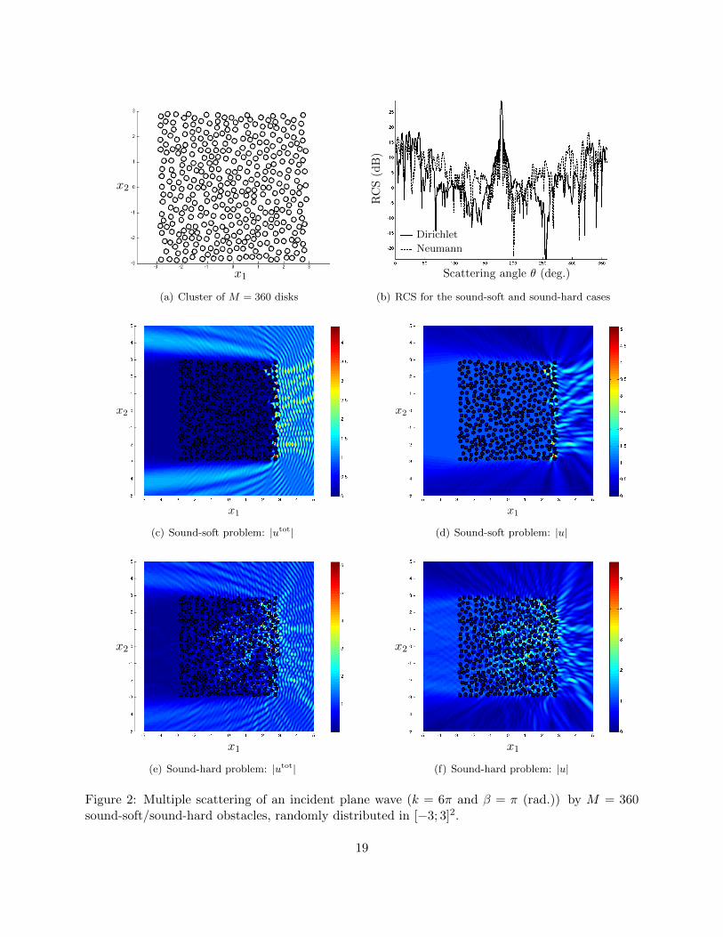
To show an example of problem solved by µ-diff, we consider that we use the EFIE to solve thescattering problem by a collection of sound-soft or sound-hard randomly distributed scatterers.The corresponding script (BenchmarkDN) for simulating the results of this section is available in theexamples directory.

We consider a plane wave (for a wavenumber k = 6π and an incidence angle β = π (rad.))that scatterers on a collection of M = 360 circular cylinders (see figure 2(a)). These disks arerandomly distributed in a square computational domain [−3; 3]2. In addition, their radii are suchthat amin := 10−1 6 ap 6 amax := 1.5 × 10−1, the minimal distance between the disks is dmin :=0.01 × amin. The number of modes is fixed by the formula (8), taken from (21) in [3]. The traceand normal derivative trace of the incident plane wave are then defined to build the right-hand

17

sides of the EFIE. We report in figure 2(b) the RCS for the sound-soft and sound-hard acousticproblems. These pictures show that the far-fields have some very different structures. In addition,the amplitudes of total and scattered wavefields are displayed on figures 2(c)-2(d) for the sound-soft problem and figures 2(e)-2(f) for the sound-hard problem. We consider a larger computationaldomain to show the wavefield behavior both inside and outside the cluster of circular cylinders. Weobserve in particular that there is almost no penetration of the incident field in the sound-soft casewhile scattering arises deeply in the sound-hard cluster.

7.2 Example II: multiple scattering by a cluster of homogeneous penetrableobstacles

Extending the previous example, the script BenchmarkPenetrable solves the transmission problemwith penetrable obstacles. The wavenumber k is now piecewise constant with value k+ outside theobstacles and k− inside. The scattered field u+ and the transmitted wavefield u− are then thesolution to the following transmission boundary-value problem

∆u− + (k−)2u− = 0, in Ω−,∆u+ + (k+)2u+ = 0, in Ω+,

u+ − u− = −uinc, on Γ,∂nu

+ − ∂nu− = −∂nuinc, on Γ,

lim||x||→+∞

||x||1/2(∇u+ · x

||x||− iku

)= 0.

(13)

The total (physical) field utot is given by utot = u+ +uinc outside and by utot = u− inside the obsta-cles. To solve this problem through an integral equation, we consider a single-layer representationof the wavefields u+ and u−

u+ = L +ρ+ and u− = L −ρ−, (14)

where L + (resp. L −) is the single-layer operator with wavenumber k+ (respectively k−). Thepair of unknowns (ρ+, ρ−) is then the solution to the following integral equation L+ −L−

−I2

+N+

(I

2+N−

) ( ρ+

ρ−

)=

(−uinc

−∂nuinc

).

The plus or minus superscripts in L and N refers to as the exterior wavenumbers k+ or k−. Like forthe sound-soft and sound-hard scattering problems, the far-field and the quantities u+ and u− can becomputed, thanks to their respective single-layer representation (14). Let us remark that the presentproblem also arises for electromagnetic wave scattering by dielectric obstacles. The wavenumbersare then given by k+ = ω

√ε0µ0 and k−p = ω

√εpµp, where ω is the pulsation of the wave and (ε0, µ0)

(respectively (εp, µp)) are respectively the electric permittivity and electromagnetic permeability inthe vacuum (respectively in the obstacle Ωp). The equation (13) remains the same except for thefourth line which is now: ∂nu

+− µ∂nu− = −∂nuinc, on Γ, where µ|Ωp = µp. As a consequence, theintegral equation in only changed by multiplying (I/2 +N−) by the parameter µ.

A numerical example solved by µ-diff is shown in figures 3(a)-3(d) for M = 400 unit penetrableunitary disks placed as a rectangular lattice centered on (0, 0), which is also the location of a point

18

x1

x2

(a) Cluster of M = 360 disks

Scattering angle θ (deg.)

RC

S(d

B)

Dirichlet

Neumann

(b) RCS for the sound-soft and sound-hard cases

x1

x2

(c) Sound-soft problem: |utot|

x1

x2

(d) Sound-soft problem: |u|

x1

x2

(e) Sound-hard problem: |utot|

x1

x2

(f) Sound-hard problem: |u|

Figure 2: Multiple scattering of an incident plane wave (k = 6π and β = π (rad.)) by M = 360sound-soft/sound-hard obstacles, randomly distributed in [−3; 3]2.

19

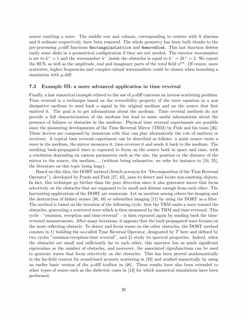
source emitting a wave. The middle row and column, corresponding to centers with 0 abscissaand 0 ordinate respectively, have been removed. The whole geometry has been built thanks to thepre-processing µ-diff functions RectangularLattice and RemoveDisk. This last function deleteseasily some disks in a geometrical configuration if they are not needed. The exterior wavenumberis set to k+ = 1 and the wavenumber k− inside the obstacles is equal to k− = 2k+ = 2. We reportthe RCS, as well as the amplitude, real and imaginary parts of the total field utot. Of course, morescatterers, higher frequencies and complex-valued wavenumbers could be chosen when launching asimulation with µ-diff.

7.3 Example III: a more advanced application in time reversal

Finally, a last numerical example related to the use of µ-diff concerns an inverse scattering problem.Time reversal is a technique based on the reversibility property of the wave equation in a nondissipative medium to send back a signal in the original medium and on the source that firstemitted it. The goal is to get informations about the medium. Time reversal methods do notprovide a full characterization of the medium but lead to some useful informations about thepresence of failures or obstacles in the medium. Physical time reversal experiments are possiblesince the pioneering developments of the Time Reversal Mirror (TRM) by Fink and his team [26].These devices are composed by numerous cells that can play alternatively the role of emitters orreceivers. A typical time reversal experiment can be described as follows: a point source emits awave in the medium, the mirror measures it, time-reverses it and sends it back to the medium. Theresulting back-propagated wave is expected to focus on the source both in space and time, witha resolution depending on various parameters such as the size, the position or the distance of themirror to the source, the medium,. . . (without being exhaustive, we refer for instance to [10, 25],the literature on this topic being huge).

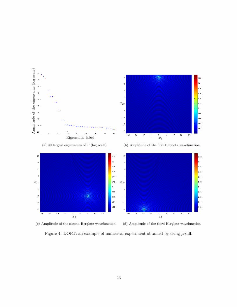
Based on this idea, the DORT method (french acronym for “Decomposition of the Time ReversalOperator”), developed by Prada and Fink [27, 43], aims to detect and locate non-emitting objects.In fact, this technique go further than the pure detection since it also generates waves that focusselectively on the obstacles that are supposed to be small and distant enough from each other. Thefascinating applications of the DORT are numerous. Let us mention among others the imaging andthe destruction of kidney stones [38, 48] or subsurface imaging [11] by using the DORT as a filter.The method is based on the iteration of the following cycle: first the TRM emits a wave toward theobstacles, generating a scattered wave which is then measured by the TRM and time-reversed. Thiscycle - ”emission, reception and time-reversal” - is then repeated again by sending back the time-reversed measurements. After many iterations, it appears that the back propagated wave focuses onthe most reflecting obstacle. To detect and focus waves on the other obstacles, the DORT methodconsists in 1) building the so-called Time Reversal Operator, designated by T here and defined bytwo cycles ”emission-reception-time reversal”, and 2) study its spectral properties. Indeed, whenthe obstacles are small and sufficiently far to each other, this operator has as much significanteigenvalues as the number of obstacles, and moreover, the associated eigenfunctions can be usedto generate waves that focus selectively on the obstacles. This has been proved mathematicallyin the far-field context for sound-hard acoustic scattering in [32] and studied numerically by usingan earlier basic version of the µ-diff toolbox in [46]. These results have also been extended toother types of waves such as the dielectric cases in [13] for which numerical simulations have beenperformed.

20

Scattering angle θ (deg.)

RC

S(d

B)

(a) RCS for the penetrable case

x1

x2

(b) Penetrable problem:∣∣utot

∣∣

x1

x2

(c) Penetrable problem: <(utot)

x1

x2

(d) Penetrable problem: =(utot)

Figure 3: Scattering of a point source (located at the origin) by a collection of M = 400 penetrableunit disks (interior wavenumber k− = 2k, with the exterior wavenumber k = 1).

21

For the sake of simplicity, we only present here the acoustic far-field case, even if the scriptsfor the two cases are available in the Examples/TimeReversal/FarField directory of the currentµ-diff toolbox. For this case, the time reversal mirror is placed at infinity and totally surroundsthe obstacles. In particular, this implies that the TRM sends a linear combination of plane waves,called Herglotz waves, and measures the scattered far-field. More precisely, an Herglotz wave uIwith parameter f is given by

uI(x1, x2) =

∫ 2π

0f(α)eik(x1 cos(α)+x2 sin(α)) dα.

Let us denote by Ff the far-field generated by an Herglotz wavefield of parameter f . Then, itcan be proved [32] that the TRO is given by: T = F∗F , where F∗ is the adjoint operator of F .An eigenfunction g of T can then be used as a parameter of an Herglotz wavefunction to generatea wave focusing on the obstacles if its associated eigenvalue is significantly large. In the discretecontext, building the matrix T associated with the operator T can be done as follows. First, theTRM is discretized by using Nα points or angles αj , j = 1, ..., Nα (note that, if a point emits anincident wave with angle α, then the TRM measures the far-field in the opposite direction α+ π).A discrete Herglotz wave emitted by the mirror is then

uI(x1, x2) =

Nα∑j=1

hαfjeik(x1 cos(αj)+x2 sin(αj)),

where fj = f(αj) and hα is the discretization step. The algorithm to obtain the time reversalmatrix T is then : for every angle αj , the scattered field is computed and the associated far-fieldis stored in a matrix F(:, j) of size Nα ×Nα. Once F has been computed, the matrix T is obtained

by the relation: T = FTF.All the elementary operations described above can be easily coded by using µ-diff and the

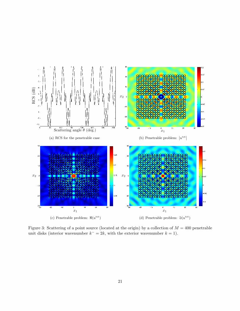
Matlab function eigen which provides the eigenvalues and eigenvectors of T. The Herglotz wavesare computed thanks to the function HerglotzWave available in the µ-diff directory related tothe examples. Finally, running the script DORT Impenetrable.m generates a DORT experiment.An example is given on figures 4(a)-4(d). We consider a medium with three penetrable circularscatterers, with centers [0, 20], [10,−10], [−10,−20] and respective radius 0.02, 0.01, 0.005. Thewavenumber is equal to k = 2π. As shown on figure 4(a), the time reversal matrix T has threesignificant eigenvalues. We report on figures 4(b)-4(d) the amplitude of the Herglotz wavefunctionsassociated with the three largest eigenvalues. We clearly observe that they selectively focus on theobstacles, from the most to the less reflecting (or largest) one.

8 Conclusion

This paper presented a new flexible, efficient and robust Matlab toolbox called µ-diff2. This opensource code is based on the theory of integral representations for solving two-dimensional multiplescattering problems by many circular cylinders. The spectral approximation method uses Fourierseries expansion and efficient linear algebra algorithms in conjunction with optimized memory

2http://mu-diff.math.cnrs.fr

22

Eigenvalue label

Am

pli

tud

eof

the

eige

nva

lue

(log

scale

)

(a) 40 largest eigenvalues of T (log scale)

x1

x2

(b) Amplitude of the first Herglotz wavefunction

x1

x2

(c) Amplitude of the second Herglotz wavefunction

x1

x2

(d) Amplitude of the third Herglotz wavefunction

Figure 4: DORT: an example of numerical experiment obtained by using µ-diff.

23

storage techniques for solving the finite-dimensional approximate integral formulations. Pre- andpost-processing facilities are included in µ-diff (near- and far-fields representations, surface fields).All the features are described with enough details so that the user can directly solve complexproblems related to physics or engineering applications. In addition, we provide some benchmarkscripts that reproduce the simulations shown in this paper (direct and inverse scattering). Theµ-diff toolbox is developed in such a way that a wide class of multiple scattering problems by diskscan be solved.

Acknowledgments. This work has been funded by the Institute of Scientific Research andRevival of Islamic Heritage at Umm Al-Qura University (project ID 43405027) and the FrenchNational Agency for Research (ANR) (project MicroWave NT09 460489).

References

[1] S. Acosta. On-surface radiation condition for multiple scattering of waves. Computer Methodsin Applied Mechanics and Engineering, in press, 2014.

[2] S. Acosta and V. Villamizar. Coupling of Dirichlet-to-Neumann boundary condition andfinite difference methods in curvilinear coordinates for multiple scattering. J. Comput. Phys.,229(5498-5517), 2010.

[3] X. Antoine, C. Chniti, and K. Ramdani. On the numerical approximation of high-frequencyacoustic multiple scattering problems by circular cylinders. J. Comput. Phys., 227(3):1754–1771, 2008.

[4] X. Antoine and M. Darbas. Alternative integral equations for the iterative solution of acousticscattering problems. Quaterly J. Mech. Appl. Math., 1(58):107–128, 2005.

[5] X. Antoine and M. Darbas. Generalized combined field integral equations for the iterativesolution of the three-dimensional Helmholtz equation. M2AN Math. Model. Numer. Anal.,1(41):147–167, 2007.

[6] X. Antoine and M. Darbas. Integral Equations and Iterative Schemes for Acoustic ScatteringProblems. to appear, 2014.

[7] X. Antoine, C. Geuzaine, and K. Ramdani. Wave Propagation in Periodic Media - Analysis,Numerical Techniques and Practical Applications, volume 1, chapter Computational Methodsfor Multiple Scattering at High Frequency with Applications to Periodic Structures Calcula-tions, pages 73–107. Progress in Computational Physics, 2010.

[8] X. Antoine, K. Ramdani, and B. Thierry. Wide frequency band numerical approaches formultiple scattering problems by disks. J. Algorithms Comput. Technol., 6(2):241–259, 2012.

[9] S. Bidault, F.J.G. de Abajo, and A. Polman. Plasmon-based nanolenses assembled on a well-defined DNA template. Journal of the American Chemical Society, 130(9):2750+, 2008.

[10] L. Borcea, G. Papanicolaou, and C. Tsogka. A resolution study for imaging and time reversalin random media. In Inverse problems: theory and applications (Cortona/Pisa, 2002), volume333 of Contemp. Math., pages 63–77. Amer. Math. Soc., Providence, RI, 2003.

24

[11] L. Borcea, G. Papanicolaou, and C. Tsogka. Adaptive time-frequency detection and filteringfor imaging in heavy clutter. SIAM J. Imaging Sciences, 4(3):827–849, 2011.

[12] H. Brakhage and P. Werner. Uber das Dirichletsche Aussenraumproblem fur die HelmholtzscheSchwingungsgleichung. Arch. Math., 16:325–329, 1965.

[13] C. Burkard, A. Minut, and K. Ramdani. Far field model for time reversal and application toselective focusing on small dielectric inhomogeneities. Inverse Problems and Imaging, 7(2):445–470, 2013.

[14] A. J. Burton and G. F. Miller. The application of integral equation methods to the numericalsolution of some exterior boundary-value problems. Proc. Roy. Soc. London. Ser. A, 323:201–210, 1971. A discussion on numerical analysis of partial differential equations (1970).

[15] M. Cassier and C. Hazard. Multiple scattering of acoustic waves by small sound-soft obstaclesin two dimensions: Mathematical justification of the Foldy-Lax model. Wave Motion, 50(18-28), 2013.

[16] J.T. Chen, Y.T. Lee, Y.J. Lin, I.L. Chen, and J.W. Lee. Scattering of sound from pointsources by multiple circular cylinders using addition theorem and superposition technique.Numerical Methods for Partial Differential Equations, 27(1365-1383), 2011.

[17] D. Colton and R. Kress. Inverse Acoustic and Electromagnetic Scattering Theory, volume 93of Applied Mathematical Sciences. Springer-Verlag, Berlin, second edition, 1998.

[18] D. L. Colton and R. Kress. Integral Equation Methods in Scattering Theory. Pure and AppliedMathematics (New York). John Wiley & Sons Inc., New York, 1983. A Wiley-IntersciencePublication.

[19] A. Devilez, B. Stout, N. Bonod, and E. Popov. Spectral analysis of three-dimensional photonicjets. Optics Express, 16(18):14200–14212, 2008.

[20] T.E. Doyle, D.A. Robinson, S.B. Jones, K.H. Warnick, and B.L. Carruth. Modeling thepermittivity of two-phase media containing monodisperse spheres: Effects of microstructureand multiple scattering. Physical Review B, 76(5), 2007.

[21] T.E. Doyle, A.T. Tew, K.H. Warnick, and B.L. Carruth. Simulation of elastic wave scatteringin cells and tissues at the microscopic level. Journal of the Acoustical Society of America,125(3):1751–1767, 2009.

[22] M. Ehrhardt. Wave Propagation in Periodic Media Analysis, Numerical Techniques and prac-tical Applications, E-Book Series Progress in Computational Physics (PiCP), Volume 1. Ben-tham Science Publishers, 2010.

[23] M. Ehrhardt, H. Han, and C. Zheng. Numerical simulation of waves in periodic structures.Commun. Comput. Phys., 5:849–870, 2009.

[24] P. Ferrand, J. Wenger, A. Devilez, M. Pianta, B. Stout, N. Bonod, E. Popov, and H. Rigneault.Direct imaging of photonic nanojets. Optics Express, 16(10):6930–6940, 2008.

25

[25] M. Fink. Time-reversal acoustics. In Inverse problems, multi-scale analysis and effectivemedium theory, volume 408 of Contemp. Math., pages 151–179. Amer. Math. Soc., Providence,RI, 2006.

[26] M. Fink. Time-reversal acoustics. J. Phys.: Conf. Ser., 118(1):012001, 2008.

[27] M. Fink and C. Prada. Eigenmodes of the time-reversal operator: A solution to selectivefocusing in multiple-target media. Wave Motion, 20:151–163, 1994.

[28] C. Geuzaine, O. Bruno, and F. Reitich. On the O(1) solution of multiple-scattering prob-lems. IEEE Trans. Magn., 41(5):1488–1491, May 2005. 11th IEEE Biennial Conference onElectromagnetic Field Computation, Seoul, South Korea, June 06-09, 2004.

[29] L. Greengard and V. Rokhlin. A fast algorithm for particle simulations. J. Comput. Phys.,73(2):325–348, 1987.

[30] M.J. Grote and C. Kirsch. Dirichlet-to-Neumann boundary conditions for multiple scatteringproblems. J. Comput. Phys., 201(2):630 – 650, 2004.

[31] R.F. Harrington and J.R. Mautz. H-field, E-field and combined field solution for conductingbodies of revolution. Archiv Elektronik und Uebertragungstechnik, 4(32):157–164, 1978.

[32] C. Hazard and K. Ramdani. Selective acoustic focusing using time-harmonic reversal mirrors.SIAM J. Appl. Math., 64(3):1057–1076, 2004.

[33] P. Hewageegana and V. Apalkov. Second harmonic generation in disordered media: Randomresonators. Physical Review B, 77(7), 2008.

[34] Z. Hu and Y.Y. Lu. Compact wavelength demultiplexer via photonic crystal multimode res-onators. J. Opt. Soc. Amer. B, to appear 2014.

[35] R.D. Meade J.D. Joannopoulos and J.N. Winn. Photonic Crystals: Molding the Flow of Light.Princeton University Press, 1995.

[36] A.A. Kharlamov and P. Filip. Generalisation of the method of images for the calculation ofinviscid potential flow past several arbitrarily moving parallel circular cylinders. Journal ofEngineering Mathematics, 77(1), 2012.

[37] P. A. Martin. Multiple Scattering. Interaction of Time-Harmonic Waves with N Obstacles,volume 107 of Encyclopedia of Mathematics and its Applications. Cambridge University Press,Cambridge, 2006.

[38] T.D. Mast, A.I. Nachman, and R.C. Waag. Focusing and imaging using the eigenfunctions ofthe scattering operator. J. Acoust. Soc. Am., 102:715–725, 1997.

[39] H. Mertens, A. F. Koenderink, and A. Polman. Plasmon-enhanced luminescence near noble-metal nanospheres: Comparison of exact theory and an improved Gersten and Nitzan model.Physical Review B, 76(11), 2007.

[40] D.M. Natarov, V.O. Byelobrov, R. Sauleau, T.M. Benson, and A.I. Nosich. Periodicity-inducedeffects in the scattering and absorption of light by infinite and finite gratings of circular silvernanowires. Optics Express, 19(22176-22190), 2011.

26

[41] J.-C. Nedelec. Acoustic and Electromagnetic Equations. Integral Representations for HarmonicProblems, volume 144 of Applied Mathematical Sciences. Springer-Verlag, New York, 2001.

[42] O.K. Pashaev and O. Yilmaz. Power-series solution for the two-dimensional inviscid flow witha vortex and multiple cylinders. Journal of Engineering Mathematics, 65(2), 2009.

[43] C. Prada. The D.O.R.T. method. J. Acoust. Soc. Am., 101(5):3090–3090, 1997.

[44] Y. Saad. Iterative Methods for Sparse Linear Systems. PWS Publishing Company Boston,1996.

[45] R. Savo, M. Burresi, T. Svensson, K. Vynck, and D.S. Wiersma. Walk dimension for light incomplex disordered media. Phys. Rev. A, 90:023839, Aug 2014.

[46] B. Thierry. Analyse et Simulations Numeriques du Retournement Temporel et de la DiffractionMultiple. Nancy University, These de Doctorat, 2011.

[47] B. Thierry. A remark on the single scattering preconditioner applied to boundary integralequations. Journal of Mathematical Analysis and Applications, 413(1):212 – 228, 2014.

[48] J.-L. Thomas, F. Wu, and M. Fink. Time reversal focusing applied to lithotripsy. UltrasonicImaging, 18(2):106–121, 1996.

[49] L. Tsang, J.A. Kong, K.H. Ding, and C.O. Ao. Scattering of Electromagnetic Waves, NumericalSimulation. Wiley Series in Remote Sensing. J.A. Kong, Series Editor, 2001.

[50] S. Tulu and O. Yilmaz. Motion of vortices outside a cylinder. Chaos, 20(4), 2010.

[51] B. Van Genechten, B. Bergen, D. Vandepitte, and W. Desmet. A Trefftz-based numericalmodelling framework for Helmholtz problems with complex multiple-scatterer configurations.J. Comput. Phys., 229(6623-6643), 2010.

[52] D.S. Wiersma. Disordered photonics. Nature Photonics, 7:188–196, Feb 2013.

27