dietrich˜von˜rosen bilinear regression analysis
TRANSCRIPT

Lecture Notes in Statistics 220
Dietrich von Rosen
Bilinear Regression AnalysisAn Introduction

Lecture Notes in Statistics 220Edited by P. Bickel, P. Diggle, S.E. Fienberg, U. Gather,S. Zeger

More information about this series at http://www.springer.com/series/694

Dietrich von Rosen
Bilinear Regression AnalysisAn Introduction
123

Dietrich von RosenDepartment of Energy and TechnologySwedish University of Agricultural SciencesUppsala, Sweden
ISSN 0930-0325 ISSN 2197-7186 (electronic)Lecture Notes in StatisticsISBN 978-3-319-78782-4 ISBN 978-3-319-78784-8 (eBook)https://doi.org/10.1007/978-3-319-78784-8
Library of Congress Control Number: 2018943157
Mathematics Subject Classification (2010): 62H12, 62H15, 62H99, 62J20, 15A69, 15A03, 15A63
© Springer International Publishing AG, part of Springer Nature 2018This work is subject to copyright. All rights are reserved by the Publisher, whether the whole or part ofthe material is concerned, specifically the rights of translation, reprinting, reuse of illustrations, recitation,broadcasting, reproduction on microfilms or in any other physical way, and transmission or informationstorage and retrieval, electronic adaptation, computer software, or by similar or dissimilar methodologynow known or hereafter developed.The use of general descriptive names, registered names, trademarks, service marks, etc. in this publicationdoes not imply, even in the absence of a specific statement, that such names are exempt from the relevantprotective laws and regulations and therefore free for general use.The publisher, the authors and the editors are safe to assume that the advice and information in this bookare believed to be true and accurate at the date of publication. Neither the publisher nor the authors orthe editors give a warranty, express or implied, with respect to the material contained herein or for anyerrors or omissions that may have been made. The publisher remains neutral with regard to jurisdictionalclaims in published maps and institutional affiliations.
Printed on acid-free paper
This Springer imprint is published by the registered company Springer International Publishing AG partof Springer NatureThe registered company address is: Gewerbestrasse 11, 6330 Cham, Switzerland

To
Tatjana,
Alexander, Evelina, Michael,Philip, Sophie

Preface
This book can be regarded as a textbook on bilinear regression analysis which couldbe used for a second course on classical multivariate analysis. The first course insuch a series would deal with multivariate linear models, focusing, for example,on the estimation of parameters and the testing of hypotheses in such models.However, the book definitely does not require any knowledge of PCA, PCR, PLS,factor analysis, cluster analysis, multidimensional scaling, etc., since it does nottreat any of these methods or any related methods. The most important prerequisiteis some knowledge of linear models (univariate and/or multivariate models), andsome knowledge of the basics of linear algebra would be helpful. The book hasbeen written for PhD students in mathematical statistics or statistics, but researcherswill probably also find some of the presented ideas and results to be of interest.The main purpose of writing this book was to present basic statistical theory forbilinear models, extending linear models theory, which from a theoretical point ofview is a big and relevant step to take. For example, we mainly deal with non-linear estimators where the estimators of the mean parameters are not independentof the estimators of the dispersion parameters. Statistics goes hand in hand withdata analysis. Therefore, one of the topics included in the book is the analysis ofresiduals, and it is emphasized that residuals are very important quantities to study.Moreover, the problem of the influence of observations is treated with some care.Generally speaking, a major part of the book includes tools that have been developedfor handling bilinear regression models from a practical perspective.
One can view the approach adopted in the book as a combination of solidmathematics and illustrative and intuitive derivations, employing examples and puredata analysis, and to some extent, this reflects my view of statistical thinking. Oneof the cornerstones of the book is the definition of models which permit a clearmathematical treatment, including the estimation of unknown parameters, togetherwith the presentation of methods for model validation against data.
It is worth noting that in several places in the book only the most enthusiasticreader will follow the details, and in fact, there are many places where the readerhas to work out the details by themselves. For example, concerning several “momentcalculations”, only a few intermediate hints are presented together with the final
vii

viii Preface
result. The same can be said about the “matrix differentiation” which is performed.If all the details had been given, I believe the technical side of the material wouldhave taken too much space. However, without any techniques it is difficult to derivenew results. My intention has been that readers should be able to identify the ideasbehind the different approaches presented in the book and should also be able tocopy the included calculations.
The book is not meant to provide easy reading. However, if one is willingto devote time and effort to working with the material, one can expect to berewarded. Students should perhaps read the book in a manner similar to jumpingon a trampoline. One’s first jump on a trampoline is not high, one’s second jumpis higher and then, in a short time, one approaches the maximum height. Thereare different thresholds to be crossed, but after a while readers will understand thelogic and basic ideas used in the book. One can also compare reading the book totravelling on a safari which at the beginning takes one through a landscape filledwith trees and bushes severely obstructing one’s view, after which one reaches asavannah, with an open landscape offering an excellent view of numerous excitinganimals.
The whole book can be studied within the framework of a two-semester coursewhich also includes solving some of the suggested problems, which can verywell be worked on in pairs. Note that some problems take quite a long time tosolve. Another alternative is to use the material in the first three chapters for acourse comprising, for example, 10 seminars, leading to knowledge about maximumlikelihood estimation in bilinear regression models (BRM) and extended bilinearregression models. A third alternative is to consider only the BRM , i.e. the growthcurve model (GMANOVA), in each of the eight chapters. This would probably leadto a course which takes a somewhat longer time to complete than one semester. Ifdesired one could reduce the course length by omitting Chap. 8, or Chaps. 7 and 8.
The structure of the book deserves a few comments. In the main body of thetext, few technical derivations are given if the results are available in the literature.Instead, the reader is referred to the appendices, where notations and technicalresults are presented. For proofs of many of the results, however, one is referred toother sources where detailed proofs can be found. Concerning the literature reviewsat the end of each chapter, I have attempted to trace early references, and it isfascinating to see how much was accomplished and understood a long time ago.It is beyond my competence, from a statistics point of view, to provide a historicalperspective on the material, but I hope that some readers will delve deeper into theearly works, with a view to understanding the conceptual core of statistics and howto transmit achieved knowledge to the next generation of scientists. The problemsthat we face today can be solved better once we have apprehended how peoplewere thinking in the pre-PC era. Moreover, I have tried to cite the literature whichis directly connected to the content of this book, but I am convinced that I haveomitted important references which I do not know of or have merely missed duringthe writing process. I would be happy to receive information about such omissions.
This book owes a great deal to many friends and colleagues. I am withoutdoubt most indebted to my wife, Tatjana, who encouraged me to start this project

Preface ix
and with whose blessing a large amount of my time has been invested in. It hasbeen a long journey which has lasted for many years, and I am happy that ithas come to an end. My colleagues and friends Kai-Tai Fang, Tõnu Kollo andMuni Srivastava have all been very important for my view of statistics in generaland multivariate analysis in particular. I have learnt a great deal from our jointlywritten articles and a book written together with Tõnu Kollo. For example, someof the material in this book stems from our collaborative works on Edgeworth-type expansions and mean shift analysis, as well as influence analysis in general.Over the years, many PhD students have contributed to discussions which havehelped me to understand various ideas implemented in this book. In particular, Ihave borrowed ideas and material produced by Jemila Hamid (on residual analysis)and Chengcheng Hao (on perturbation analysis). Furthermore, special thanks areextended to Martin Singull, with whom I have shared the supervision of severalPhD students and have had numerous discussions on topics related to this book. I amgrateful to Thomas Holgersson who unselfishly spent time reading a draft versionof the book. Thanks also go to Katarzyna Filipiak and Augustyn Markiewicz fororganizing and inviting me to a very interesting workshop series in Bedlewo, Poland(the Mathematical Research and Conference Center (MRCC) which is part of theInstitute of Mathematics of the Polish Academy of Sciences). I have visited theworkshops an uncountable number of times, and the stimulating discussions and the“free thinking environment” have had a great impact on this book. At the very endof this project, Paul McMillen made a complete linguistic revision and I am boththankful for and impressed by his improvement of the English of the manuscript.Finally, I would like to acknowledge gratefully all those (who are too many to belisted) who have helped me by providing references and shedding light on detailedconcerns which I have had over the years.
I would be grateful to be informed of any errors which readers might find in thebook. The responsibility for the errors is, of course, mine alone.
Uppsala, Sweden Dietrich von RosenNovember 2017

Contents
1 Introduction . . . . . . . . . . . . . . . . . . . . . . . . . . . . . . . . . . . . . . . . . . . . . . . . . . . . . . . . . . . . . . . . . . 11.1 What Is Statistics . . . . . . . . . . . . . . . . . . . . . . . . . . . . . . . . . . . . . . . . . . . . . . . . . . . . . . 11.2 What Is a Statistical Model. . . . . . . . . . . . . . . . . . . . . . . . . . . . . . . . . . . . . . . . . . . . 21.3 The General Univariate Linear Model with a Known Dispersion . . . 61.4 The General Multivariate Linear Model . . . . . . . . . . . . . . . . . . . . . . . . . . . . . . 111.5 Bilinear Regression Models: An Introduction .. . . . . . . . . . . . . . . . . . . . . . . 13Problems .. . . . . . . . . . . . . . . . . . . . . . . . . . . . . . . . . . . . . . . . . . . . . . . . . . . . . . . . . . . . . . . . . . . . . . 25Literature . . . . . . . . . . . . . . . . . . . . . . . . . . . . . . . . . . . . . . . . . . . . . . . . . . . . . . . . . . . . . . . . . . . . . . 26References . . . . . . . . . . . . . . . . . . . . . . . . . . . . . . . . . . . . . . . . . . . . . . . . . . . . . . . . . . . . . . . . . . . . . 32
2 The Basic Ideas of Obtaining MLEs: A Known Dispersion . . . . . . . . . . . . . 392.1 Introduction . . . . . . . . . . . . . . . . . . . . . . . . . . . . . . . . . . . . . . . . . . . . . . . . . . . . . . . . . . . . 392.2 Linear Models with a Focus on the Singular Gauss-Markov
Model. . . . . . . . . . . . . . . . . . . . . . . . . . . . . . . . . . . . . . . . . . . . . . . . . . . . . . . . . . . . . . . . . . . 392.3 Multivariate Linear Models . . . . . . . . . . . . . . . . . . . . . . . . . . . . . . . . . . . . . . . . . . . 492.4 BRM with a Known Dispersion Matrix . . . . . . . . . . . . . . . . . . . . . . . . . . . . . . 502.5 EBRMm
B with a Known Dispersion Matrix . . . . . . . . . . . . . . . . . . . . . . . . . . 532.6 EBRMm
W with a Known Dispersion Matrix. . . . . . . . . . . . . . . . . . . . . . . . . . 62Problems .. . . . . . . . . . . . . . . . . . . . . . . . . . . . . . . . . . . . . . . . . . . . . . . . . . . . . . . . . . . . . . . . . . . . . . 65Literature . . . . . . . . . . . . . . . . . . . . . . . . . . . . . . . . . . . . . . . . . . . . . . . . . . . . . . . . . . . . . . . . . . . . . . 66References . . . . . . . . . . . . . . . . . . . . . . . . . . . . . . . . . . . . . . . . . . . . . . . . . . . . . . . . . . . . . . . . . . . . . 68
3 The Basic Ideas of Obtaining MLEs: Unknown Dispersion. . . . . . . . . . . . . 713.1 Introduction . . . . . . . . . . . . . . . . . . . . . . . . . . . . . . . . . . . . . . . . . . . . . . . . . . . . . . . . . . . . 713.2 BRM and Its MLEs . . . . . . . . . . . . . . . . . . . . . . . . . . . . . . . . . . . . . . . . . . . . . . . . . . . 713.3 EBRM3
B and Its MLEs . . . . . . . . . . . . . . . . . . . . . . . . . . . . . . . . . . . . . . . . . . . . . . . 793.4 EBRM3
W and Its MLEs . . . . . . . . . . . . . . . . . . . . . . . . . . . . . . . . . . . . . . . . . . . . . . . 853.5 Reasons for Using Both the EBRM3
B and the EBRM3W . . . . . . . . . . . 90
Problems .. . . . . . . . . . . . . . . . . . . . . . . . . . . . . . . . . . . . . . . . . . . . . . . . . . . . . . . . . . . . . . . . . . . . . . 91Literature . . . . . . . . . . . . . . . . . . . . . . . . . . . . . . . . . . . . . . . . . . . . . . . . . . . . . . . . . . . . . . . . . . . . . . 92References . . . . . . . . . . . . . . . . . . . . . . . . . . . . . . . . . . . . . . . . . . . . . . . . . . . . . . . . . . . . . . . . . . . . . 95
xi

xii Contents
4 Basic Properties of Estimators . . . . . . . . . . . . . . . . . . . . . . . . . . . . . . . . . . . . . . . . . . . . . 994.1 Introduction . . . . . . . . . . . . . . . . . . . . . . . . . . . . . . . . . . . . . . . . . . . . . . . . . . . . . . . . . . . . 994.2 Asymptotic Properties of Estimators of Parameters in the BRM . . . 1014.3 Moments of Estimators of Parameters in the BRM . . . . . . . . . . . . . . . . . 1044.4 EBRM3
B and Uniqueness Conditions for MLEs. . . . . . . . . . . . . . . . . . . . . 1194.5 Asymptotic Properties of Estimators of Parameters
in the EBRM3B . . . . . . . . . . . . . . . . . . . . . . . . . . . . . . . . . . . . . . . . . . . . . . . . . . . . . . . . 123
4.6 Moments of Estimators of Parameters in the EBRM3B . . . . . . . . . . . . . . 128
4.7 EBRM3W and Uniqueness Conditions for MLEs . . . . . . . . . . . . . . . . . . . . 157
4.8 Asymptotic Properties of Estimators of Parametersin the EBRM3
W . . . . . . . . . . . . . . . . . . . . . . . . . . . . . . . . . . . . . . . . . . . . . . . . . . . . . . . . 1594.9 Moments of Estimators of Parameters in the EBRM3
W . . . . . . . . . . . . . 160Problems .. . . . . . . . . . . . . . . . . . . . . . . . . . . . . . . . . . . . . . . . . . . . . . . . . . . . . . . . . . . . . . . . . . . . . . 172Literature . . . . . . . . . . . . . . . . . . . . . . . . . . . . . . . . . . . . . . . . . . . . . . . . . . . . . . . . . . . . . . . . . . . . . . 173References . . . . . . . . . . . . . . . . . . . . . . . . . . . . . . . . . . . . . . . . . . . . . . . . . . . . . . . . . . . . . . . . . . . . . 174
5 Density Approximations . . . . . . . . . . . . . . . . . . . . . . . . . . . . . . . . . . . . . . . . . . . . . . . . . . . . . 1775.1 Introduction . . . . . . . . . . . . . . . . . . . . . . . . . . . . . . . . . . . . . . . . . . . . . . . . . . . . . . . . . . . . 1775.2 Preparation . . . . . . . . . . . . . . . . . . . . . . . . . . . . . . . . . . . . . . . . . . . . . . . . . . . . . . . . . . . . . 1785.3 Density Approximation for the Mean Parameter in the BRM . . . . . . 1855.4 Density Approximation for the Mean Parameter Estimators
in the EBRM3B . . . . . . . . . . . . . . . . . . . . . . . . . . . . . . . . . . . . . . . . . . . . . . . . . . . . . . . . 192
5.5 Density Approximation for the Mean Parameter Estimatorsin the EBRM3
W . . . . . . . . . . . . . . . . . . . . . . . . . . . . . . . . . . . . . . . . . . . . . . . . . . . . . . . . 206Problems .. . . . . . . . . . . . . . . . . . . . . . . . . . . . . . . . . . . . . . . . . . . . . . . . . . . . . . . . . . . . . . . . . . . . . . 215Literature . . . . . . . . . . . . . . . . . . . . . . . . . . . . . . . . . . . . . . . . . . . . . . . . . . . . . . . . . . . . . . . . . . . . . . 216References . . . . . . . . . . . . . . . . . . . . . . . . . . . . . . . . . . . . . . . . . . . . . . . . . . . . . . . . . . . . . . . . . . . . . 218
6 Residuals . . . . . . . . . . . . . . . . . . . . . . . . . . . . . . . . . . . . . . . . . . . . . . . . . . . . . . . . . . . . . . . . . . . . . . 2216.1 Introduction . . . . . . . . . . . . . . . . . . . . . . . . . . . . . . . . . . . . . . . . . . . . . . . . . . . . . . . . . . . . 2216.2 Residuals for the BRM . . . . . . . . . . . . . . . . . . . . . . . . . . . . . . . . . . . . . . . . . . . . . . . 2256.3 Distribution Approximations of the Residuals in the BRM . . . . . . . . . 2316.4 Mean Shift Evaluations of the Residuals in the BRM . . . . . . . . . . . . . . . 2376.5 Residual Analysis for R1 in the BRM . . . . . . . . . . . . . . . . . . . . . . . . . . . . . . . 2516.6 Residuals for the EBRM3
B . . . . . . . . . . . . . . . . . . . . . . . . . . . . . . . . . . . . . . . . . . . . 2566.7 Residuals for the EBRM3
W . . . . . . . . . . . . . . . . . . . . . . . . . . . . . . . . . . . . . . . . . . . 267Problems .. . . . . . . . . . . . . . . . . . . . . . . . . . . . . . . . . . . . . . . . . . . . . . . . . . . . . . . . . . . . . . . . . . . . . . 276Literature . . . . . . . . . . . . . . . . . . . . . . . . . . . . . . . . . . . . . . . . . . . . . . . . . . . . . . . . . . . . . . . . . . . . . . 277References . . . . . . . . . . . . . . . . . . . . . . . . . . . . . . . . . . . . . . . . . . . . . . . . . . . . . . . . . . . . . . . . . . . . . 279
7 Testing Hypotheses . . . . . . . . . . . . . . . . . . . . . . . . . . . . . . . . . . . . . . . . . . . . . . . . . . . . . . . . . . . 2817.1 Introduction . . . . . . . . . . . . . . . . . . . . . . . . . . . . . . . . . . . . . . . . . . . . . . . . . . . . . . . . . . . . 2817.2 Background . . . . . . . . . . . . . . . . . . . . . . . . . . . . . . . . . . . . . . . . . . . . . . . . . . . . . . . . . . . . 2817.3 Likelihood Ratio Testing, H0 : FBG = 0, in the BRM . . . . . . . . . . . . 286

Contents xiii
7.4 Likelihood Ratio Testing H0 : F 1BG1 = 0 in the BRM
with the Restrictions F 2BG2 = 0, C(F ′1) ⊆ C(F ′
2) . . . . . . . . . . . . . . . . . 2997.5 Likelihood Ratio Testing H0 : F 2BG2 = 0 in the BRM
with the Restrictions F 1BG1 = 0, C(F ′1) ⊆ C(F ′
2) andC(G2) ⊆ C(G1) . . . . . . . . . . . . . . . . . . . . . . . . . . . . . . . . . . . . . . . . . . . . . . . . . . . . . . . . 306
7.6 Likelihood Ratio Testing H0 : F iBGi = 0, i = 1, 2,Against B Unrestricted in the BRM with C(F ′
1) ⊆ C(F ′2) . . . . . . . . . 312
7.7 Likelihood Ratio Testing H0 : F iBGi = 0, i = 1, 2,Against B Unrestricted in the BRM with C(F ′
1) ⊆ C(F ′2)
and C(G2) ⊆ C(G1) . . . . . . . . . . . . . . . . . . . . . . . . . . . . . . . . . . . . . . . . . . . . . . . . . . . 3177.8 A “Trace Test” for the BRM , H0 : FBG = 0 Against
Unrestricted B . . . . . . . . . . . . . . . . . . . . . . . . . . . . . . . . . . . . . . . . . . . . . . . . . . . . . . . . . 3237.9 A “Trace Test” for the BRM , H0 : F iBGi = 0, i = 1, 2,
C(F ′1) ⊆ C(F ′
2), Against Unrestricted B . . . . . . . . . . . . . . . . . . . . . . . . . . . . . 3377.10 The Likelihood Ratio Test Versus the “Trace Test” . . . . . . . . . . . . . . . . . . 3427.11 Testing an EBRM3
B Against a BRM . . . . . . . . . . . . . . . . . . . . . . . . . . . . . . . . 3437.12 Estimating and Testing in the BRM with F 1BG1 = F 2�G2 . . . . . 350Problems .. . . . . . . . . . . . . . . . . . . . . . . . . . . . . . . . . . . . . . . . . . . . . . . . . . . . . . . . . . . . . . . . . . . . . . 354Literature . . . . . . . . . . . . . . . . . . . . . . . . . . . . . . . . . . . . . . . . . . . . . . . . . . . . . . . . . . . . . . . . . . . . . . 355References . . . . . . . . . . . . . . . . . . . . . . . . . . . . . . . . . . . . . . . . . . . . . . . . . . . . . . . . . . . . . . . . . . . . . 358
8 Influential Observations . . . . . . . . . . . . . . . . . . . . . . . . . . . . . . . . . . . . . . . . . . . . . . . . . . . . . 3638.1 Introduction . . . . . . . . . . . . . . . . . . . . . . . . . . . . . . . . . . . . . . . . . . . . . . . . . . . . . . . . . . . . 3638.2 Influence Analysis in Univariate Linear Models . . . . . . . . . . . . . . . . . . . . . 3658.3 Influence Analysis in the BRM . . . . . . . . . . . . . . . . . . . . . . . . . . . . . . . . . . . . . . . 3738.4 Influence Analysis in the EBRM3
B . . . . . . . . . . . . . . . . . . . . . . . . . . . . . . . . . . . 3938.5 Influence Analysis in the EBRM3
W . . . . . . . . . . . . . . . . . . . . . . . . . . . . . . . . . . 407Problems .. . . . . . . . . . . . . . . . . . . . . . . . . . . . . . . . . . . . . . . . . . . . . . . . . . . . . . . . . . . . . . . . . . . . . . 413Literature . . . . . . . . . . . . . . . . . . . . . . . . . . . . . . . . . . . . . . . . . . . . . . . . . . . . . . . . . . . . . . . . . . . . . . 413References . . . . . . . . . . . . . . . . . . . . . . . . . . . . . . . . . . . . . . . . . . . . . . . . . . . . . . . . . . . . . . . . . . . . . 417
Appendices . . . . . . . . . . . . . . . . . . . . . . . . . . . . . . . . . . . . . . . . . . . . . . . . . . . . . . . . . . . . . . . . . . . . . . . . 423Appendix A: Notation. . . . . . . . . . . . . . . . . . . . . . . . . . . . . . . . . . . . . . . . . . . . . . . . . . . . . . . . . 423Appendix B: Useful Technical Results . . . . . . . . . . . . . . . . . . . . . . . . . . . . . . . . . . . . . . . 431Problems .. . . . . . . . . . . . . . . . . . . . . . . . . . . . . . . . . . . . . . . . . . . . . . . . . . . . . . . . . . . . . . . . . . . . . . 448Appendix C: Test Statistics . . . . . . . . . . . . . . . . . . . . . . . . . . . . . . . . . . . . . . . . . . . . . . . . . . . 450References . . . . . . . . . . . . . . . . . . . . . . . . . . . . . . . . . . . . . . . . . . . . . . . . . . . . . . . . . . . . . . . . . . . . . 455
Subject Index . . . . . . . . . . . . . . . . . . . . . . . . . . . . . . . . . . . . . . . . . . . . . . . . . . . . . . . . . . . . . . . . . . . . . 457
Index – Theorems and Corollaries . . . . . . . . . . . . . . . . . . . . . . . . . . . . . . . . . . . . . . . . . . . . . 463
Index – Figures and Tables . . . . . . . . . . . . . . . . . . . . . . . . . . . . . . . . . . . . . . . . . . . . . . . . . . . . . . 467

Chapter 1Introduction
1.1 What Is Statistics
Statistical science is about planning experiments, setting up models to analyseexperiments and observational studies, and studying the properties of these modelsor the properties of some specific building blocks within these models, e.g.parameters and independence assumptions. Statistical science also concerns thevalidation of chosen models, often against data. Statistical application is aboutconnecting statistical models to data.
The general statistical paradigm is based on the following steps:
1. setting up a model;2. evaluating the model via simulations or comparisons with data;3. if necessary, refining the model and restarting from step 2;4. accepting and interpreting the model.
There is indeed also a step 0, namely determining the source of inspiration forsetting up a statistical model. At least two cases can be identified: (i) the data-inspired model, i.e. depending on our experiences and what is seen in data, a modelis formulated; (ii) the conceptually inspired model, i.e. someone has an idea aboutwhat the relevant components are and how these components should be included inthe model of some process, for example.
It is obvious that when applying the paradigm, a number of decisions have tobe made which unfortunately are all rather subjective. This should be taken intoaccount when relying on statistics. Moreover, if statistics is to be useful, the modelshould be relevant for the problem under consideration, which is often relative tothe information which can be derived from the data, and the final model should beinterpretable. Statistics is instrumental, since, without expertise in the discipline inwhich it is applied, one usually cannot draw firm conclusions about the data whichare used to evaluate the model. On the other hand, “data analysts”, when applyingstatistics, need a solid knowledge of statistics to be able to perform efficient analysis.
© Springer International Publishing AG, part of Springer Nature 2018D. von Rosen, Bilinear Regression Analysis, Lecture Notes in Statistics 220,https://doi.org/10.1007/978-3-319-78784-8_1
1

2 1 Introduction
The purpose of this book is to provide tools for the treatment of the so-called bilinearmodels. Bilinear models are models which are linear in two “directions”. A typicalexample of something which is bilinear is the transformation of a matrix into anothermatrix, because one can transform the rows as well as the columns simultaneously.In practice rows and columns can, for example, represent a “spatial” direction and a“temporal” direction, respectively.
Basic ingredients in statistics are the concept of probability and the assumptionabout the underlying distributions. The distribution is a probability measure onthe space of “random observations”, i.e. observations of a phenomenon whoseoutcome cannot be stated in advance. However, what is a probability and what doesa probability represent? Statistics uses the concept of probability as a measure ofuncertainty. The probability measures used nowadays are well defined through theircharacterization via Kolmogorov’s axioms. However, Kolmogorov’s axioms tell uswhat a probability measure should fulfil, but not what it is. It is not even obviousthat something like a probabilistic mechanism exists in real life (nature), but forstatisticians this does not matter. The probability measure is part of a model and anymodel, of course, only describes reality approximatively.
1.2 What Is a Statistical Model
A statistical model is usually a class of distributions which is specified via functionsof parameters (unknown quantities). The idea is to choose an appropriate modelclass according to the problem which is to be studied. Sometimes we know exactlywhat distribution should be used, but more often we have parameters which generatea model class, for example the class of multivariate normal distributions with anunknown mean and dispersion. Instead of distributions, it may be convenient, inparticular for interpretations, to work with random variables which are representa-tives of the random phenomenon under study, although sometimes it is not obviouswhat kind of random variable corresponds to a distribution function. In Chap. 5 ofthis book, for example, some cases where this phenomenon occurs are dealt with.One problem with statistics (in most cases only a philosophical problem) is how toconnect data to continuous random variables. In general it is advantageous to lookupon data as realizations of random variables. However, since our data points haveprobability mass 0, we cannot directly couple, in a mathematical way, continuousrandom variables to data.
There exist several well-known schools of thought in statistics advocatingdifferent approaches to the connection of data to statistical models and these schoolsdiffer in the rigour of their method. Examples of these approaches are “distribution-free” methods, likelihood-based methods and Bayesian methods. Note that the factthat a method is distribution-free does not mean that there is no assumption madeabout the model. In a statistical model there are always some assumptions aboutrandomness, for example concerning independence between random variables.Perhaps the best-known distribution-free method is the least squares approach.

1.2 What Is a Statistical Model 3
Likelihood methods utilize classes of distributions which are generated byunknown parameters and the idea is to estimate these parameters. A consequenceof this procedure is that we obtain the distribution which should be consideredthe true distribution, as well as acquiring information about the parameters which,if the model is appropriately specified, is interpretable. Concerning the normaldistribution, usually the mean and variance act as parameters, although from anexponential family point of view, a more natural equivalent parametrization can beset up.
In Bayesian methods the basic idea is that everything unknown is modelled withthe help of distributions, for instance, unknown parameters. One is avoiding some ofthe problems with the likelihood approach, such as connecting continuous data to amodel, but instead one generates other problems; for example it is difficult to specifydistributions for all the unknown elements. Moreover, in the Bayesian approachthe concept of conditional independence is crucial, in contrast to the likelihoodapproach, where independence is used. Which method is to be preferred is a matterof taste.
This book is mainly likelihood-inspired, i.e. likelihood acts as a basis for thepresentations. However, one should note that many statistical inference proceduresare not purely frequentistic, Bayesian or likelihood procedures. For example, if oneis dealing with normally distributed variables with unknown singular dispersionmatrices, it is not clear which school of thought can be adopted when trying tofollow the general statistical paradigm. Other deep discussions can concern theconcept of confidence intervals and variable selection methods. General materialof interest, including deliberations on deeper philosophical issues, are presented inEvans et al. (1986), Davison (2003), Berger and Molina (2004), Geisser (2006),Mayo and Cox (2006) and Cox (2006), for example.
In fact, in some way, restricting the inference procedures to one particularprocedure is inconsistent with the statistical paradigm. The problem at hand shouldguide one’s choice. Moreover, one has to decide if the conclusions and decisionmaking should be based on probabilistic arguments, for example hypotheses testing.In this book we emphasize understanding the statistical model and the statisticsunder consideration. For example, in the case of an estimator or a hypothesis test,we want to understand what is really being estimated or tested. The basic problem isthe difference between a statistical model and the corresponding estimated model,which is data-dependent, i.e. different data sets may lead to different interpretationsand conclusions.
Example 1.1 In this example, several statistical approaches for evaluating a modelare presented. Let
x′ = β ′C + e′,
where x : n×1, a random vector corresponding to the observations, C : k×n, is thedesign matrix, β : k × 1 is an unknown parameter vector which is to be estimated,and e ∼ Nn(0, σ 2I ), which is considered to be the error term in the model and

4 1 Introduction
where σ 2 denotes the variance, which is supposed to be unknown. In this book theterm “observation” is used in the sense of observed data which are thought to berealizations of some random process. In statistical theory the term “observation”often refers to a set of random variables. Let the projector PC ′ = C′(CC′)−C
be defined in Appendix A, Sect. A.7, where (•)− denotes an arbitrary g-inverse(see Appendix A, Sect. A.6). Some useful results for projectors are presented inAppendix B, Theorem B.11.
The least squares approach works as follows. Let xo be the observations of x,and let us minimize, with respect to β,
(x′o − E[x′])(x′
o − E[x′])′ = (x′o − β ′C)(x′
o − β ′C)′,
which yields
β′oC = x′
oP C ′, (1.1)
where βo stands for the estimate of β, i.e. an explicit numerical value of β.Moreover, it follows that
(x′o − β ′C)(x′
o − β ′C)′ = x′o(I − PC ′)xo + (x′
oPC ′ − β ′C)()′ ≥ x′o(I − PC ′)xo,
where (•)()′ is used according to Appendix A, Sect. A.7, with equality if and onlyif (1.1) is true. In order to study properties of the estimate, xo is replaced by x, andwhen doing so, the estimator
β′C = x′P C ′
is obtained. Due to the linearity of the estimator
β′C ∼ Nn(βC, σ 2P C ′);
i.e. βC is unbiased and normally distributed with variance σ 2PC ′ . The varianceparameter can be estimated as nσ 2 = x′(I − P C ′)x. According to the statisticalparadigm, models should be evaluated. The linear model in this example may, forinstance, be evaluated via residuals, i.e. x′
o(I −PC ′) and x′(I −PC ′). For example,one should validate the model with respect to influential observations and outliersas well as the fit of the model to data. Moreover, specific properties such as thesmallest variance properties of the β-estimator can be shown or the “best quadratic”properties of the variance estimator.
An alternative estimation procedure is based on finding estimators which mini-mize the overall variance
E[(x′ − β ′C)(x′ − β ′C)′],

1.2 What Is a Statistical Model 5
which can be rewritten in the following way:
E[(x′ − β ′C)(x′ − β ′C)′]= E[x′(I − P C ′)x] + E[(x′P C ′ − β ′C)(x′P C ′ − β ′C)′]. (1.2)
Thus, it follows that the estimator equals
β′C = x′P C ′,
because in this case the second term in (1.2) equals 0. In order to verify the modelvia comparisons to data, the estimate
β′oC = x′
oP C ′,
is calculated. The expressions for the estimator and estimate are the same as thecorresponding expressions in the least squares approach, although conceptually themethods differ to a great extent; i.e. for the least squares method we start with data,find an estimate and then construct an estimator by replacing the data, xo, by x.For the minimization of the variance we started with x, found an estimator and thenconstructed an estimate by replacing x by xo.
Now we turn to the likelihood approach. Here one starts with the likelihood,which nowadays, for continuous random variables, is the density of x evaluated atxo, i.e.
L(β, σ 2) = (2π)−n/2(σ 2)−n/2exp{− σ 2
2 (x′o − β ′C)(x′
o − β ′C)′}.
This function is maximized with respect to σ 2 and β which gives
β′oC = x′
oC′(CC′)−C = x′
oP C ′,
nσ 2o = x′
o(I − C′(CC′)−C)xo = x′o(I − P C ′)xo.
In a second step of the likelihood approach β is constructed by replacing xo by x.Hence, we establish that the likelihood approach will lead to the same conclusion asthe least squares and the minimum variance approaches.
��Over the years many more estimation methods have been presented. For example,shrinkage methods, robust methods and Bayesian methods. We would also liketo emphasize that models should be meaningful, i.e. that the parameters and theirestimators should be understandable, and computations connected to the modelshould be fast. The past 20 years, with the arrival of increasingly powerful PCs andcomputer facilities, have witnessed an absurd use of algorithms and one can evensee programs running for days and nights. The beauty of statistics, as well as itsrelation to mathematics, has been partly lost. This is serious, because mathematics

6 1 Introduction
helps us to examine the models and understand the analysis. Without mathematicsit is easy to become trapped in too many ad hoc procedures. Intuition and ad hocprocedures should be basic ingredients in statistical model building, but they shouldalso be possible to verify. This is the best way to create an end-product which canlater be improved. Using too many simulation studies will result in an end-productwhich only with difficulty can be transmitted to the next generation of statisticians.
This book considers models which are called bilinear. Briefly speaking, the maindifference between linear and bilinear models is that in the estimation process, thelatter uses random weights when performing projections (due to an estimated innerproduct), whereas linear models generally use non-random projections. Anotherimportant fact is that under usual normality assumptions bilinear models do notbelong to the exponential family.
1.3 The General Univariate Linear Model with a KnownDispersion
In this section the classical Gauss-Markov set-up is considered but we assumethe dispersion matrix to be completely known. If the dispersion matrix is positivedefinite (p.d.), the model is just a minor extension of the model in Example 1.1.However, if the dispersion matrix is positive semi-definite (p.s.d.), other aspectsrelated to the model will be introduced. In general, in the Gauss-Markov model thedispersion is proportional to an unknown constant, but this is immaterial for ourpresentation. The reason for investigating the model in some detail is that there hasto be a close connection between the estimators based on models with a knowndispersion and those based on models with an unknown dispersion. Indeed, if oneassumes a known dispersion matrix, all our models can be reformulated as Gauss-Markov models. With additional information stating that the random variables arenormally distributed, one can see from the likelihood equations that the maximumlikelihood estimators (MLEs) of the mean parameters under the assumption ofan unknown dispersion should approach the corresponding estimators under theassumption of a known dispersion. For example, the likelihood equation for themodel X ∼ Np,n(ABC,�, I ) which appears when differentiating with respect toB (see Appendix A, Sect. A.9 for definition of the matrix normal distribution andChap. 1, Sect. 1.5 for a precise specification of the model) equals
A′�−1(X − ABC)C′ = 0;
and for a large sample any maximum likelihood estimator of B has to satisfythis equation asymptotically, because we know that the MLE of � is a consistentestimator. For interested readers it can be worth studying generalized estimatingequation (GEE) theory, for example see Shao (2003, pp. 359–367).
Now let us discuss the univariate linear model
x′ = β ′C + e′, e ∼ Nn(0,V ), (1.3)

1.3 The General Univariate Linear Model with a Known Dispersion 7
where V : n × n is p.d. and known, x : n × 1, C : k × n and β : k × 1 is tobe estimated. Let xo, as previously, denote the observations of x and let us useV −1 = V −1P C ′,V +P (C ′)o,V −1V −1 (see Appendix B, Theorem B.13), where (C′)ois any matrix satisfying C((C′)o)⊥ = C(C′), where C(•) denotes the column vectorspace (see Appendix A, Sect. A.8). Then the likelihood is maximized as follows:
L(β) ∝ |V |−1/2exp{−1/2(x′o − β ′C)V −1(x′
o − β ′C)′}= |V |−1/2exp{−1/2(x′
oP′C ′,V − β ′C)V −1()′}
×exp{−1/2(x′oP (C ′)o,V −1V
−1xo)}≤ |V |−1/2exp{−1/2(x′
oP (C ′)o,V −1V−1xo)},
which is independent of any parameter, i.e. β, and the upper bound is attained if andonly if
β′oC = x′
oP′C ′,V ,
where βo is the estimate of β . Thus, in order to estimate β a linear equationsystem has to be solved. The solution can be written as follows (see Appendix B,Theorem B.10 (i)):
β′o = x′
oV−1C′(CV −1C ′)− + z′(C)o
′,
where z′ stands for an arbitrary vector of a proper size.Suppose that in model (1.3) there are restrictions (a priori information) on the
mean vector given by
β ′G = 0.
Then
β ′ = θ ′Go′,
where θ is a new unrestricted parameter. After inserting this relation in (1.3), thefollowing model appears:
x′ = θ ′Go′C + e′, e ∼ Nn(0,V ).
Thus, the above-presented calculations yield
β′oC = x′
oP′C ′Go,V

8 1 Introduction
and from here, since this expression constitutes a consistent linear equation in βo, ageneral expression for βo (β) can be obtained explicitly.
If V is p.s.d the likelihood does not exist and the model consists of a continuousand a discrete part. Because V is p.s.d., there exists a semi-orthogonal matrix H :n × r , where r = r(V ) and V = HH ′ (see Appendix A, Sect. A.5), such that
H o′V = 0.
Note that we do not lose any “information” if a one-to-one transformation of x
takes place. Therefore the estimation of β in (1.3) can equivalently be carried outvia x′(H : H o), where (H : H o) denotes the partitioned matrix of H and H o (seeAppendix A, Sect. A.8). Hence, with probability 1
x′oH
o = β ′CH o (1.4)
and therefore we assume (consistency assumption) H o′xo ∈ C(H o′
C′), which isequivalent to xo ∈ C(C′ : V ). Thus, the data put restrictions on β, which is a newfeature in comparison with the case when V is of full rank. The meaningfulness ofthis depends on the problem under consideration. Moreover,
x′H = β ′CH + e, e ∼ Nr(0,H ′V H ). (1.5)
Equation (1.4) is linear in β and because of consistency (see Appendix B,Theorem B.10 (i))
β ′ = x′oH
o(CH o)− + θ ′(CH o)o′,
where one can view the elements of θ as a new set of unrestricted parameters.Inserting the solution into (1.5) yields
x′H = x′oH
o(CH o)−CH + θ ′(CH o)o′CH + e.
From earlier calculations we know that
θ′o = x′
o(I − H o(CH o)−C)H
×(H ′V H )−1H ′C′(CH o)o((CH o)o′CH (H ′V H )−1H ′C′(CH o)o)−
+z′((CH o)o′CH )o
′, (1.6)
where z is an arbitrary vector and then
β′o = x′
oHo(CH o)− + x′
o(I − H o(CH o)−C)H
×(H ′V H )−1H ′C′(CH o)o((CH o)o′CH (H ′V H )−1H ′C′(CH o)o)−(CH o)o
′
+z′((CH o)o′CH )o
′(CH o)o
′.

1.3 The General Univariate Linear Model with a Known Dispersion 9
If we study the statistical properties of this estimate, we should consider thefollowing (remember (1.4) and that H ′H = I ):
β′ = β ′CH o(CH o)−
−β ′CH o(CH o)−CHH ′C′(CH o)o((CH o)o′CHH ′C′(CH o)o)−(CH o)o
′
+x′HH ′C′(CH o)o((CH o)o′CHH ′C′(CH o)o)−(CH o)o
′
+z′((CH o)o′CH )o
′(CH o)o
′
and then assume some conditions (estimability conditions) so that forβ′L, for some
specific L, the term including z will disappear. Moreover, in practice the conditionxo ∈ C(C′ : V ) may not be satisfied and then a pretreatment of data has to takeplace, for example a projection of data on the space C(C′ : V ).
Example 1.2 Here the singular Gauss-Markov model is illustrated. In an experi-ment where the eating behaviour of n dairy cows was studied in connection with theadministration of food, one could keep the total amount of food fixed (let us say t)over a 24 h day-and-night cycle. During the 24 h, a record was made of how mucheach of the n cows was eating. Due to breeding and local environmental conditions,the cows are correlated with a covariance matrix σ 2V , where σ 2 is an unknownscaling parameter. Since the cows have been part of many feeding experiments,the correlation between the cows can be supposed to be known. The main ideais to relate the recorded values to various explanatory variables, such as lactation,the amount of produced milk and variables measuring the quality of the milk. Ifthe measurements are denoted as x0i , i = 1, 2, . . . , n, and the other explanatoryvariables as c1i , c2i , . . . cki , the following linear model can be set up:
xi = μ +k
∑
j=1
βjcji + εi , i = 1, 2, . . . , n,
which in matrix notation equals
x′ = β ′C + e′;
C = (1n, c1, c2, . . . , ck)′, cj = (cji ), e ∼ Nn(0, σ 2V ), and β = (μ, β1, . . . , βk)
′and σ 2 are unknown parameters. As an estimator of σ 2 we can use
(n − k − 1)σ 2 = (x′ −β′C)()′,
for some estimatorβ of β. Thus, if we are able to estimate β, all the parameters canbe estimated.
The technical treatment of the model proceeds as follows. Note that by makinga one-to-one transformation of x, there is no information loss. Thus, x will be

10 1 Introduction
pre-multiplied by 1′ and 1o′. From the experimental assumptions it follows that
x′1 = t , which in turn implies V 1 = 0 and
β ′C1 = x′1 = t .
This means that, according to the model, we have an equation with no variation, andthus the equation can be treated as a deterministic equation which puts restrictionson β. Solving this equation (see Appendix B, Theorem B.10 (i)) leads to
β ′ = t (C1)− + θ(C1)o′,
where θ is an arbitrary vector of a proper size. Moreover,
x′1o = t (C1)−C1o + θ(C1)o′C1o + e,
where e ∼ Nn(0, 1o′V 1o). In this model the MLE is obtained via
β′C1o = t (C1)−C1o +θ(C1)o
′C1o,
where
θ(C1)o′C1o = (x′ − t (C1)−C)1o(1o′
V 1o)−11o′C′(C1)o
×((C1)o′C1o(1o′
V 1o)−11o′C′(C1)o)−(C1)o
′C1o.
from which β can be obtained under certain conditions on C. ��In the example it was supposed that x′1 = t , which implied that 1′V = 0. However,as noted above, we can assume that we have models where V is singular withoutany exact restrictions on x. When restrictions are put on the dispersion (covariance)matrix, we have restrictions on the random variable which only hold with probability1. Therefore, it must in this case also be assumed that the data belong to a propersubspace, which may indeed be difficult to verify.
Moreover, for the linear model
x′ = β ′C + e′, e = (0, σ 2V )
with restrictions
β ′K = h;
the situation can be described via the following model:
(x′ : h) = β ′(C : K) + e′, e = (0, σ 2W ),

1.4 The General Multivariate Linear Model 11
where
W =(
V 00 0
)
.
This clearly shows how general the singular Gauss-Markov model is.
1.4 The General Multivariate Linear Model
In this book we study models which are based on an underlying multivariate normaldistribution. The multivariate normal distribution is closely connected to linearity,since a linear function of a normal variable is also normally distributed. The theoryaround the normal distribution is well developed and one can, among other things,show that the general multivariate linear model under certain conditions belongsto the exponential family, which is very important. For example, for models whichbelong to the exponential family, there are complete and sufficient statistics, and allthe moments and cumulants are at our disposal.
The general multivariate linear model equals
X = BC + E, (1.7)
where X : p × n is a random matrix which corresponds to the observations, B :p × k is an unknown parameter matrix and C : k × n is a known design matrix.Furthermore, E ∼ Np,n(0,�, I ), where � is an unknown p.d. matrix. For adefinition of the matrix normal distribution Np,n(μ, •, •) see Appendix A, Sect. A.9.The model in (1.7) is also called the MANOVA model. According to the modelspecifications, the model consists of independently distributed columns. The designmatrix C is also called a between-individuals design matrix. In order to be able todraw any conclusions from the model, we have to estimate the unknown parametersB and �. Following the statistical paradigm, we also have to verify the model andthis usually takes place with the help of residuals.
If we examine the likelihood function, L(B,�), we have
L(B,�) ∝ |�|n/2exp{−1/2tr{�−1(Xo − BC)()′}}= |�|n/2exp(−1/2tr{�−1So + �−1(XoP C ′ − BC)()′}),
where
So = Xo(I − PC ′)X′o.
Let S be as So, but with Xo replaced by X. From here it follows that the modelbelongs to the exponential family and that XP C ′ and S are sufficient statistics. It

12 1 Introduction
can be shown that the statistics also are complete. The MLEs for B and � areobtained from
BoC = XoP C ′, (1.8)
n�o = So,
since (1.8) constitutes a linear consistent equation system in B. The likelihood isalways smaller or equal to (2π)−pn/2|n−1So|−n/2exp{−np/2}, where the upperbound is obtained when inserting BoC and �o.
Example 1.3 This is an example where several variables are to be modelled simul-taneously. In environmental monitoring one can use many chemical biomarkers.For example, in Sweden, one monitors calcium, magnesium, sodium, potassium,sulphate, chloride, fluoride, nitrogen, phosphorus, conductivity and other sub-stances/properties in lakes spread over the whole country. Observations are collectedseveral times over the year. Imagine that we want to compare two regions fora specific year. Then one can select 20 lakes from each region and as responsevariables use the above-mentioned chemical variables, for which an average overthe summer months can be used, for example. The model for the data with tenresponse variables and 40 observations equally divided between the two regions canbe presented in the following way:
X = BC + E,
where X: 10×40, B: 10×2 consists of the mean parameters, E ∼ N10,40(0,�, I ),where �: 10 × 10 is the unknown dispersion matrix, and
C =(
1′20 00 1′
20
)
.
��Example 1.4 Now an example with repeated measurements with an unstructuredmean is briefly presented. Another strategy for comparing regions than that pre-sented in Example 1.3 is to focus on one of the chemical variables, for examplenitrogen. Moreover, instead of averaging over the summer months as in Exam-ple 1.3, we can use the measurements from June, July and August. Thus we couldset up the following model:
X = BC + E,
where X: 3 × 40, B: 3 × 2 consists of the mean parameters, E ∼ N3,40(0,�, I ),where �: 3 × 3 is the unknown dispersion matrix, and the between-individualsdesign matrix C is as in Example 1.3. ��

1.5 Bilinear Regression Models: An Introduction 13
There are two natural follow-up questions concerning the models presented inExamples 1.3 and 1.4. The first concerns with the repeated measurements fornitrogen over the summer months. It would be of interest to use a linear modelfor these measurements, in particular if we were to include data from some moremonths. Then we would have a complete analogy with the analysis of growth curvedata, but here, instead of growth, nitrogen over time would be studied. The secondquestion is if we could analyse all ten chemical variables over time simultaneously.In that case we would have an analogy with a spatio-temporal model setting. Here,instead of geographic spatial information, we would be observing different chemicalvariables. Both these extensions would be outside the general multivariate linearmodel setting. However, under certain restrictions they could be analysed withbilinear regression models, since the mean structure, instead of being linear, wouldbe bilinear. This would imply, among other things, that the models do not belong tothe exponential family.
1.5 Bilinear Regression Models: An Introduction
Throughout the book BRM is used as an abbreviation for bilinear regression model.Other common names are the growth curve model or GMANOVA (generalizedmultivariate analysis of variance). At the end of the previous section, it was notedthat even under normality assumptions, we have very natural models which do notbelong to the exponential family. It was also noted in the previous section that if amodel has a linear mean structure, the model belongs to the exponential family. Inthis section, it will be shown, among other things, that if a bilinear mean structure isassumed together with an arbitrary dispersion matrix, the model is not a memberof the exponential family and instead belongs to the curved exponential family.Remember that if a matrix is pre- and post-multiplied by other matrices, we performa bilinear transformation.
Often the mean structure ABC is considered, where the unknown parameter isgiven by B. Hence, we have a bilinear model:
X = ABC + E, (1.9)
where X: p × n, the unknown mean parameter matrix B: q × k, the two designmatrices A: p×q and C: k×n, and the error matrix E build up the model. Moreover,let E be normally distributed with independent columns, mean 0, and a positivedefinite dispersion matrix � for the elements within each column of X. Then thedensity function for X is proportional to
|�|−1/2nexp{−1/2tr{�−1(X − ABC)(X − ABC)′}}
and after some manipulations it can be shown that this model belongs to the curvedexponential family. For example, this can be shown through a reparametrization,

14 1 Introduction
i.e. according to Appendix B, Theorem B.1 (i), A can be factored as A = �(
I0
)
T ,where � is orthogonal and T is a non-singular matrix. Moreover, let � = T B ,� = �′��, Y = �′X, Y ′ = (Y ′
1 : Y ′2) and
�−1 =(
�11 �12
�21 �22
)
.
Then the density function for the new variable Y is proportional to
|�−1|n/2exp{−1/2(tr{�−1Y (I − P C ′)Y ′} − 2tr{Y 1�11�C}
−2tr{Y 2�21�C} + tr{�11�CC′�′})},
which shows that the model belongs to the curved exponential family, since thenumber of “free” parameters, i.e. �−1 and �11�, is less than the number offunctions including observations and parameters. Note that
�21� = (I : 0)�−1(0 : I )′((I : 0)�−1(I : 0)′)−1�11�.
The above-mentioned model is often termed the growth curve model and wasintroduced by Potthoff and Roy (1964), although very similar models had beenconsidered earlier. The A matrix is often referred to as the within-individuals designmatrix and C, as in (1.7), is called the between-individuals design matrix.
A natural extension of the BRM is the following “sum of profiles” model
X =m∑
i=1
AiBiCi + E,
where X: p × n is the sample matrix, the mean parameter matrices are Bi : qi × ki ,the within-individual design matrices equal Ai : p × qi and the between-individualdesign matrices Ci : ki × n, are such that
C(C′m) ⊆ C(C′
m−1) ⊆ · · · ⊆ C(C′1). (1.10)
Let E be matrix normally distributed with independent columns, mean 0, and adispersion matrix � for the elements within each column of E. Note that insteadof (1.10), we can suppose that
C(Am) ⊆ C(Am−1) ⊆ · · · ⊆ C(A1). (1.11)
The model is referred to herein as the extended bilinear regression model (EBRM•• )
and in order to distinguish between (1.10) and (1.11), as well as indicate m inthe profile expression, EBRMm
B and EBRMmW are used, where the subscripts B
and W stand for “between” and “within”, respectively, and are used depending on

1.5 Bilinear Regression Models: An Introduction 15
whether (1.10) or (1.11) is assumed to hold. Sometimes the EBRMm• is called theextended growth curve model. The conditions in (1.10) or (1.11) are mathematicallymotivated since they lead to explicit MLEs. Concerning these conditions, there is ananalogy with the Behrens-Fisher problem; i.e. the purpose is to compare two groupsof size n1 and n2, respectively, for testing equality of the means with the additionalassumption that random variables corresponding to the observations from differentgroups have different variances, i.e.
x′ = μ′C + e′,
where μ′ = (μ′1 : μ′
2),
C =(
1′n1
⊗(
1
0
)
: 1′n2
⊗(
0
1
))
,
where ⊗ denotes the Kronecker product (see Appendix A, Sect. A.6) and
e′ ∼ Nn(0,(
σ 21 In1 00 σ 2
2 In2
)
), n = n1 + n2.
Comparing μ1 and μ2 will not give any precise answer about differences betweengroups, i.e. their distributions, unless σ 2
i is taken into account. If (1.10) or (1.11)does not hold, we have, instead of a common mean and different variances (Behrens-Fisher case), different means and a common dispersion matrix. This situation iscalled seemingly unrelated regression (SUR) and has been extensively studied in aunivariate setting (e.g. see Kariya and Kurata, 2004). An example of a univariateSUR model is the SUR model with two functionally independent regression lines,but correlated error terms. In the multivariate case it becomes more difficult tointerpret results and there are reasons why one should avoid this type of model.
This section is concluded by giving some more examples.
Example 1.5 This example illustrates the use of the BRM to analyse Swedishliming data (see also Examples 1.3 and 1.4). For many years there has been aproblem with the acidification of lakes in Sweden, and to help lakes to recover,one is liming them to stimulate the recovery process. Below we present a data setwhich covers ten lakes from each of two regions where the pH concentration hasbeen measured at three different depths, 0.5, 5 and 10 m. Since the pH is highestclose to the surface and thereafter decreases we can try to model the concentrationwith a linear model. The data are presented in Table 1.1. The following matricesare involved in the description of the data. The matrix X is the random matrixwhich corresponds to the data and X ∼ N3,20(ABC,�, I ), where B is an unknown

16 1 Introduction
Table 1.1 Selected data, with some minor modifications, from the integrated monitoring of theeffects of liming project at the Swedish University of Agricultural Sciences; pH represents minusthe decimal logarithm of the hydrogen ion activity
Lake Depth pH Region Lake Depth pH Region
1 0.5 6.72 1 11 0.5 7.29 2
1 5.0 6.61 1 11 5.0 6.78 2
1 10.0 6.41 1 11 10.0 6.76 2
2 0.5 6.80 1 12 0.5 6.91 2
2 5.0 6.80 1 12 5.0 6.91 2
2 10.0 6.70 1 12 10.0 6.71 2
3 0.5 7.16 1 13 0.5 7.23 2
3 5.0 7.12 1 13 5.0 7.37 2
3 10.0 7.01 1 13 10.0 7.10 2
4 0.5 7.17 1 14 0.5 6.81 2
4 5.0 7.20 1 14 5.0 6.68 2
4 10.0 7.08 1 14 10.0 6.18 2
5 0.5 6.96 1 15 0.5 6.66 2
5 5.0 6.68 1 15 5.0 6.47 2
5 10.0 6.48 1 15 10.0 6.17 2
6 0.5 7.23 1 16 0.5 6.89 2
6 5.0 7.02 1 16 5.0 6.59 2
6 10.0 6.80 1 16 10.0 6.19 2
7 0.5 6.87 1 17 0.5 6.98 2
7 5.0 6.73 1 17 5.0 6.64 2
7 10.0 6.43 1 17 10.0 6.24 2
8 0.5 7.15 1 18 0.5 6.88 2
8 5.0 7.18 1 18 5.0 7.01 2
8 10.0 6.80 1 18 10.0 6.71 2
9 0.5 7.23 1 19 0.5 7.01 2
9 5.0 7.03 1 19 5.0 6.90 2
9 10.0 6.73 1 19 10.0 6.80 2
10 0.5 7.24 1 20 0.5 7.20 2
10 5.0 7.19 1 20 5.0 7.17 2
10 10.0 6.99 1 20 10.0 7.07 2
parameter matrix and � is p.d. but unstructured, and where
A =⎛
⎝
1 0.51 51 10
⎞
⎠ , C =(
1′10 ⊗
(
1
0
)
: 1′10 ⊗
(
0
1
))
. ��
Example 1.6 This example concerns the hormone melatonin and acute severedepression. More than 30 years ago, depression was already being studiedconcerning its relation to various hormones, in particular melatonin. Among other

1.5 Bilinear Regression Models: An Introduction 17
8 10 12 14 16 18 20 22 24 2 4 6 8
nmol/l
Time of Day
0.1
0.2
0.3
Melaton
in
Fig. 1.1 Serum melatonin levels patients with acute depression (∗) and a control group of healthyindividuals (+). Group-averaged sample means have been joined in the figure
discoveries, the melatonin peak level was found to be lowered in patients sufferingfrom acute depression in comparison to the corresponding level in healthy subjects.The melatonin levels for these two groups are shown in Fig. 1.1. The peak levelsremained low when these patients were re-examined during remission. Therefore,melatonin levels can be viewed as a bio-marker for depression. It is typical ofmelatonin, as well as some other hormones (e.g. cortisol), that they follow a day-and-night cycle.
If the data consist of ten repeated measurements over the day-and-night cycle,the following model can be used: X ∼ N10,60(ABC,�, I ), where (ω = π/24)
A =
⎛
⎜
⎜
⎜
⎜
⎜
⎜
⎜
⎜
⎜
⎜
⎜
⎜
⎝
1 sin(ω) cos(ω) sin(2ω) cos(2ω)
1 sin(4ω) cos(4ω) sin(4 ∗ 2ω) cos(4 ∗ 2ω)
1 sin(8ω) cos(8ω) sin(8 ∗ 2ω) cos(8 ∗ 2ω)
1 sin(12ω) cos(12ω) sin(12 ∗ 2ω) cos(12 ∗ 2ω)
1 sin(14ω) cos(14ω) sin(14 ∗ 2ω) cos(14 ∗ 2ω)
1 sin(16ω) cos(16ω) sin(16 ∗ 2ω) cos(16 ∗ 2ω)
1 sin(18ω) cos(18ω) sin(18 ∗ 2ω) cos(18 ∗ 2ω)
1 sin(20ω) cos(20ω) sin(20 ∗ 2ω) cos(20 ∗ 2ω)
1 sin(22ω) cos(22ω) sin(22 ∗ 2ω) cos(22 ∗ 2ω)
1 sin(24ω) cos(24ω) sin(24 ∗ 2ω) cos(24 ∗ 2ω)
⎞
⎟
⎟
⎟
⎟
⎟
⎟
⎟
⎟
⎟
⎟
⎟
⎟
⎠
,
C =(
1′28 ⊗
(
1
0
)
: 1′32 ⊗
(
0
1
))
,
i.e. there are two groups (28 patients and 32 healthy controls, which are supposedto follow the mean structure indicated in Fig. 1.1). ��Example 1.7 This is an additional example illustrating the application of the BRM ,utilizing the classical dental data set of Potthoff and Roy (1964). The data consist ofgrowth measurements, i.e. the distance in mm from the centre of the pituitary to the

18 1 Introduction
pterygomaxillary fissure, for 11 girls and 16 boys at ages t1 = 8, t2 = 10, t3 = 12and t4 = 14. The design matrices equal
A1 =
⎛
⎜
⎜
⎝
1 t1
1 t2
1 t3
1 t4
⎞
⎟
⎟
⎠
, Linear growth; A2 =
⎛
⎜
⎜
⎝
1 t1 t21
1 t2 t22
1 t3 t23
1 t4 t24
⎞
⎟
⎟
⎠
, Quadratic growth;
C =(
1′11 ⊗
(
1
0
)
: 1′16 ⊗
(
0
1
))
.
Then, the model is given by either X ∼ N4,27(A1BC,�, I ) or X ∼N4,27(A2BC,
�, I ). The data are presented in Table 1.2 and illustrated in Fig. 1.2. One can observethat there is a difference between the boys and girls, and in subsequent sectionswe are going to investigate if there is a statistical model which can be used in theanalyses, including a validation of the model, and where the difference between thegenders can be tested. ��
Table 1.2 Four repeated growth measurements were taken at ages t1 = 8, t2 = 10, t3 = 12 andt4 = 14 from 11 girls and 16 boys (by permission of Potthoff and Roy (1964) © Oxford UniversityPress 1964)
Id Gender t1 t2 t3 t4 Id Gender t1 t2 t3 t4
1 F 21.0 20.0 21.5 23.0 12 M 26.0 25.0 29.0 31.0
2 F 21.0 21.5 24.0 25.5 13 M 21.5 22.5 23.0 26.5
3 F 20.5 24.0 24.5 26.0 14 M 23.0 22.5 24.0 27.5
4 F 23.5 24.5 25.0 26.5 15 M 25.5 27.5 26.5 27.0
5 F 21.5 23.0 22.5 23.5 16 M 20.0 23.5 22.5 26.0
6 F 20.0 21.0 21.0 22.5 17 M 24.5 25.5 27.0 28.5
7 F 21.5 22.5 23.0 25.0 18 M 22.0 22.0 24.5 26.5
8 F 23.0 23.0 23.5 24.0 19 M 24.0 21.5 24.5 25.5
9 F 20.0 21.0 22.0 21.5 20 M 23.0 20.5 31.0 26.0
10 F 16.5 19.0 19.0 19.5 21 M 27.5 28.0 31.0 31.5
11 F 24.5 25.0 28.0 28.0 22 M 23.0 23.0 23.5 25.0
23 M 21.5 23.5 24.0 28.0
24 M 17.0 24.5 26.0 29.5
25 M 22.5 25.5 25.5 26.0
26 M 23.0 24.5 26.0 30.0
27 M 22.0 21.5 23.5 25.0

1.5 Bilinear Regression Models: An Introduction 19
Age
8 10 12 14
15
20
25
30
Distancein
mm.
Fig. 1.2 The distance in mm from the centre of the pituitary to the pterygomaxillary fissure ingirls (solid line) and boys (dashed line) at ages 8, 10, 12 and 14
Example 1.8 Now an example illustrating the applications of the EBRM3B is
presented. Let us start from the very beginning and suppose that we have a randomvector x associated with observations which follow the model
x = μ + e,
where e ∼ Np(0,�). Assume that there exists a linear relation between thecomponents in μ, i.e. μ ∈ C(A). Thus, μ = Aβ for some β (see Appendix B,Theorem B.3 (i)) and x = Aβ + e. Moreover, suppose that we have n independentobservations which all have the same within-individuals model μ ∈ C(A), andsuppose that there additionally exists a linear model between the independentobservations. For example, there are three groups of individuals one correspondingto a group receiving a placebo treatment and the others corresponding to groupsreceiving two different treatments. Thus we end up with the following model:
X = ABC + E,
where X = (x1, x2, . . . , xn), B = (β1,β2,β3), E ∼ Np,n(0,�, I ) and
C =⎛
⎝
1 1 . . . 1 0 0 . . . 0 0 0 . . . 00 0 . . . 0 1 1 . . . 1 0 0 . . . 00 0 . . . 0 0 0 . . . 0 1 1 . . . 1
⎞
⎠ .

20 1 Introduction
Furthermore, assume that we have a polynomial growth. Then the Vandermondematrix, for example,
A =
⎛
⎜
⎜
⎜
⎜
⎝
1 t1 . . . tq−11
1 t2 . . . tq−12
......
. . ....
1 tp . . . tq−1p
⎞
⎟
⎟
⎟
⎟
⎠
describes the connection between growth and time. In this model all the individualsfollow the same polynomial growth model. However, if each treatment groupfollows a polynomial of a different order, we may, for example, have the followingmodel:
X = A1B1C1 + A2B2C2 + A3B3C3 + E,
where
C1 =⎛
⎝
1 1 . . . 1 0 0 . . . 0 0 0 . . . 00 0 . . . 0 1 1 . . . 1 0 0 . . . 00 0 . . . 0 0 0 . . . 0 1 1 . . . 1
⎞
⎠ ,
C2 =(
1 1 . . . 1 0 0 . . . 0 0 0 . . . 00 0 . . . 0 1 1 . . . 1 0 0 . . . 0
)
,
C3 = (
1 1 . . . 1 0 0 . . . 0 0 0 . . . 0)
,
A1 =
⎛
⎜
⎜
⎜
⎜
⎝
1 t1 . . . tq−31
1 t2 . . . tq−32
......
. . ....
1 tp . . . tq−3p
⎞
⎟
⎟
⎟
⎟
⎠
, B1 = (β1,β2,β3),
A′2 =
(
tq−21 t
q−22 . . . t
q−2p
)
, B2 = (β3, β4),
A′3 =
(
tq−11 t
q−12 . . . t
q−1p
)
, B3 = β5.

1.5 Bilinear Regression Models: An Introduction 21
Note that C(C′3) ⊆ C(C′
2) ⊆ C(C′1). The above example implies, for instance, that
the mean of the placebo group and that of the treatment groups, respectively, equal
β11 + β12t + · · · + β1(q−2)tq−3,
β21 + β22t + · · · + β2(q−2)tq−3 + β2(q−1)t
q−2,
β31 + β32t + · · · + β3(q−2)tq−3 + β3(q−1)t
q−2 + β3qtq−1.
��Example 1.9 In order to illustrate certain ideas, the “real” example presented asExample 1.6 is now extended to form Example 1.9. An additional purpose of thisis to present the ingredients for performing simulation studies which, several times,will take place later in this book. Suppose that there are three treatment groupscomprising 10, 15 and 20 patients. The groups are assumed to follow differentmodels over the day-and-night cycle, according to a nested subspace assumption:
X = A1B1C1 + A2B2C2 + A3B3C3 + E,
E ∼ Np,n(0,�, I ), C(C′3) ⊆ C(C′
2) ⊆ C(C′1),
where (ω = π/24),
A1 =
⎛
⎜
⎜
⎜
⎜
⎜
⎜
⎜
⎜
⎜
⎜
⎜
⎜
⎜
⎜
⎝
1 sin(ω) cos(ω)
1 sin(4ω) cos(4ω)
1 sin(8ω) cos(8ω)
1 sin(12ω) cos(12ω)
1 sin(14ω) cos(14ω)
1 sin(16ω) cos(16ω)
1 sin(18ω) cos(18ω)
1 sin(20ω) cos(20ω)
1 sin(22ω) cos(22ω)
1 sin(24ω) cos(24ω)
⎞
⎟
⎟
⎟
⎟
⎟
⎟
⎟
⎟
⎟
⎟
⎟
⎟
⎟
⎟
⎠
, A2 =
⎛
⎜
⎜
⎜
⎜
⎜
⎜
⎜
⎜
⎜
⎜
⎜
⎜
⎜
⎜
⎝
sin(2ω)
sin(4 ∗ 2ω)
sin(8 ∗ 2ω)
sin(12 ∗ 2ω)
sin(14 ∗ 2ω)
sin(16 ∗ 2ω)
sin(18 ∗ 2ω)
sin(20 ∗ 2ω)
sin(22 ∗ 2ω)
sin(24 ∗ 2ω)
⎞
⎟
⎟
⎟
⎟
⎟
⎟
⎟
⎟
⎟
⎟
⎟
⎟
⎟
⎟
⎠
, A3 =
⎛
⎜
⎜
⎜
⎜
⎜
⎜
⎜
⎜
⎜
⎜
⎜
⎜
⎜
⎜
⎝
cos(2ω)
cos(4 ∗ 2ω)
cos(8 ∗ 2ω)
cos(12 ∗ 2ω)
cos(14 ∗ 2ω)
cos(16 ∗ 2ω)
cos(18 ∗ 2ω)
cos(20 ∗ 2ω)
cos(22 ∗ 2ω)
cos(24 ∗ 2ω)
⎞
⎟
⎟
⎟
⎟
⎟
⎟
⎟
⎟
⎟
⎟
⎟
⎟
⎟
⎟
⎠
,
C1 = (1′10 ⊗
⎛
⎜
⎝
1
0
0
⎞
⎟
⎠ : 1′15 ⊗
⎛
⎜
⎝
0
1
0
⎞
⎟
⎠ : 1′20 ⊗
⎛
⎜
⎝
0
0
1
⎞
⎟
⎠),
C2 = (1′10 ⊗
(
1
0
)
: 1′15 ⊗
(
0
1
)
: 1′20 ⊗
(
0
0
)
), C3 = (1′10 : 1′
35 ⊗ 0).

22 1 Introduction
Here C(C′3) ⊆ C(C′
2) ⊆ C(C′1) is satisfied and in order to generate data, the
remaining task is to specify the parameters:
B1 =⎛
⎝
0.01 0.14 0.200.21 −0.01 −0.0040.02 0.03 −0.01
⎞
⎠ , B2 = (−0.04 −0.06)
, B3 = (0.10),
102�
=
⎛
⎜
⎜
⎜
⎜
⎜
⎜
⎜
⎜
⎜
⎜
⎜
⎜
⎝
0.25 −0.10 0.10 −0.10 0.10 0.20 0.05 0.00 −0.05 0.05−0.10 0.29 −0.14 0.09 −0.04 −0.13 −0.07 0.05 0.07 −0.02
0.10 −0.14 0.33 −0.01 0.04 0.15 −0.01 0.03 0.11 0.12−0.10 0.09 −0.01 0.31 0.01 −0.13 −0.09 −0.03 0.11 0.05
0.10 −0.04 0.04 0.01 0.21 0.03 0.01 0.03 −0.05 0.030.20 −0.13 0.15 −0.13 0.03 0.45 0.10 0.05 0.03 0.050.05 −0.07 −0.01 −0.09 0.01 0.10 0.30 0.00 −0.15 0.130.00 0.05 0.03 −0.03 0.03 0.05 0.00 0.21 0.07 −0.11
−0.05 0.07 0.11 0.11 −0.05 0.03 −0.15 0.07 0.28 −0.060.05 −0.02 0.12 0.05 0.03 0.05 0.13 −0.11 −0.06 0.34
⎞
⎟
⎟
⎟
⎟
⎟
⎟
⎟
⎟
⎟
⎟
⎟
⎟
⎠
.
The choice of parameters is directed by the values presented in Fig. 1.3. In thisfigure two groups of individuals follow a day-and-night cycle, whereas in the presentexample a third group of individuals has been added which does not show anynocturnal peak level (see Fig. 1.3). Later, in Sect. 6.6, the data will be contaminatedand the effect of this contamination on various residuals will be studied. ��
8 10 12 14 16 18 20 22 24 2 4 6 8
Time of Day
0.1
0.15
0.2
Fig. 1.3 Based on the serum melatonin data presented in Example 1.6 a new data set with threegroups of individuals has been generated. Group 1, Group 2 and Group 3 are indicated by asterisksymbol, plus symbol and open circle, respectively, and follow the model in Example 1.9

1.5 Bilinear Regression Models: An Introduction 23
Example 1.10 The model in Example 1.8 is now reconsidered. This exampleindicates how the EBRM3
B and EBRM3W are related. However, in general the
relation between the EBRM3B and EBRM3
W is not so clear. The following modelis equivalent to the model in Example 1.8:
X = A1�1C1 + A2�2C2 + A3�3C3 + E,
where
C1 = (
1 1 . . . 1 0 0 . . . 0 0 0 . . . 0)
,
C2 = (
0 0 . . . 0 1 1 . . . 1 0 0 . . . 0)
,
C3 = (
0 0 . . . 0 0 0 . . . 0 1 1 . . . 1)
,
A1 =
⎛
⎜
⎜
⎜
⎜
⎝
1 t1 . . . tq−11
1 t2 . . . tq−12
......
. . ....
1 tp . . . tq−1p
⎞
⎟
⎟
⎟
⎟
⎠
, �1 = (β ′1, β3, β5)
′,
A2 =
⎛
⎜
⎜
⎜
⎜
⎝
1 t1 . . . tq−21
1 t2 . . . tq−22
......
. . ....
1 tp . . . tq−2p
⎞
⎟
⎟
⎟
⎟
⎠
, �2 = (β ′2, β4)
′,
A3 =
⎛
⎜
⎜
⎜
⎜
⎝
1 t1 . . . tq−31
1 t2 . . . tq−32
......
. . ....
1 tp . . . tq−3p
⎞
⎟
⎟
⎟
⎟
⎠
, �3 = β3.
The interesting point is that now C(A3) ⊆ C(A2) ⊆ C(A1) holds instead ofC(C′
3) ⊆ C(C′2) ⊆ C(C′
1). Moreover, when considering the EBRM3B , {B i},
i = 1, 2, 3, are the objects of interest, whereas in the EBRM3W the parameters
{�i}, i = 1, 2, 3, are of interest. For example, if the estimability conditions areconsidered, the estimability of B1 does not necessarily imply the estimability of�1. Of course, if {Bi} is estimable, then so too are {�i}, i = 1, 2, 3, but usuallywe are not interested in estimating all the parameters in {Bi}, i = 1, 2, 3, uniquelyand then it is not so easy to find out the estimability conditions for �i . Moreover,

24 1 Introduction
deriving D[�i ] from D[Bi ] without knowledge about the covariance C[B i ,Bj ],i �= j , is impossible (see Appendix A, Sect. A.10 for definitions of these moments).
��The next example involves a relatively complicated between-individuals design,together with an easily interpretable within-individuals structure.
Example 1.11 EBRM3W : This example presents a so-called interference model,
see Filipiak and von Rosen (2012) and Filipiak and Markiewicz (2017), among otherpresentations. Consider an agricultural experiment and suppose that one wants tocompare t different varieties of spring barley, for example. There is likely to be aninteraction between the environment (the type of soil, rainfall, drainage, etc.) and thevariety of grain which will affect the yield. Therefore, b blocks are chosen wherethe environment is fairly consistent throughout the blocks.
Let n experimental units (plots) be divided into the b blocks each of size k. Letthe t treatments be applied to the units so that each unit receives one treatment. Thetreatment which is applied to unit j in block i is determined by the design d . Withinthe blocks the effect of the treatments applied to each unit can be quantified via arandom variable x.
Assume that the response of a given plot may be affected by treatments ofneighbouring plots, as well as by the treatment applied to that plot. Moreover,consider experiments with a one-dimensional arrangement of plots in each block,and in which the treatments have different left and right neighbour interferenceeffects.
The linear model associated with the design d can be written as follows:
x′ = β1C1,d + β2C2,d + β3C3 + e′, (1.12)
where βi , i = 1, 2, 3, are the unknown vectors of treatment effects, neighboureffects and block effects, respectively, and e is the vector of random errors. Thematrix C1,d ∈ R
v×n depends on the design and it is a matrix with binary entrieswhich satisfies C′
1,d1v = 1n. The matrix C′2,d = ((I b ⊗ H )C′
1,d : (I b ⊗ H ′)C′1,d)
is a known matrix of neighbour effects, where
H ′ =(
0′k−1 1Ik−1 0k−1
)
or H′ =(
0′k−1 0Ik−1 0k−1
)
for a circular design (Druilhet, 1999) and for a design without border plots (Kunertand Martin, 2000), respectively (0k−1 is a k − 1 dimensional vector of zeros). Thematrix C3 = I b ⊗ 1′
k is the design matrix of block effects. In the literature sucha model as the one presented above is called an interference model with neighboureffects.
Suppose that for each treatment, we are measuring a response which consistsof p characteristics. Then the following extension of the interference model (1.12)

1.5 Bilinear Regression Models: An Introduction 25
appears:
X = A1B1C1,d + A2B2C2,d + A3B3C3 + E,
where X ∈ Rp×n is the matrix of observations, B i , i = 1, 2, 3, are the unknown
matrices of treatment, neighbour and block effects, respectively, and Ai , i = 1, 2, 3,are within-individuals design matrices, which now will be specified. It is assumedthat in the experiment there is no left- and right-neighbour effect and no blockeffect for the last characteristic, and for the second last characteristic there is noblock effect. Then A1 = Ip, A2 = (Ip−1, 0p−1)
′ and A3 = (Ip−2, 0p−2, 0p−2)′,
which obviously satisfy C(A3) ⊆ C(A2) ⊆ C(A1). Finally it is noted that E ∼Np,n(0,�, I ), where � > 0 is an unstructured dispersion matrix. ��
Problems
1 Generate data according to X ∼ N5,20(ABC,�, I 20), where
A =
⎛
⎜
⎜
⎜
⎜
⎜
⎝
1 2 41 3 91 4 161 5 251 6 36
⎞
⎟
⎟
⎟
⎟
⎟
⎠
, � =
⎛
⎜
⎜
⎜
⎜
⎜
⎝
3.0 1.0 0.5 0.5 1.01.0 4.0 1.5 1.5 1.00.5 1.5 2.0 1.0 0.50.5 1.5 1.0 2.0 0.51.0 1.0 0.5 0.5 2.0
⎞
⎟
⎟
⎟
⎟
⎟
⎠
, B =(
1 0.53 4
)
C =(
1 1 1 1 1 1 1 1 1 1 0 0 0 0 0 0 0 0 0 00 0 0 0 0 0 0 0 0 0 1 1 1 1 1 1 1 1 1 1
)
.
Present informative plot(s) of the data.
2 Let xi ∼ N5(μ,�), i = 1, . . . , n, be independently distributed, where
μ =
⎛
⎜
⎜
⎜
⎜
⎜
⎝
12453
⎞
⎟
⎟
⎟
⎟
⎟
⎠
, � =
⎛
⎜
⎜
⎜
⎜
⎜
⎝
4.0 2.0 1.5 2.5 1.02.0 5.0 0.5 2.5 2.01.5 0.5 2.0 1.0 0.52.5 2.5 2.0 2.0 1.51.0 2.0 0.5 1.5 3.0
⎞
⎟
⎟
⎟
⎟
⎟
⎠
.
Put
μ = 1
n
n∑
i=n
xi .

26 1 Introduction
(i) Formulate the weak law of large numbers, i.e. μ converges in probability toμ, and indicate through simulations that the error is of order n−1. (ii) Formulate themultivariate central limit theorem, i.e. μ converges in distribution to the multivariatenormal distribution, and indicate through simulations that the error is of order n−1/2.
3 (i) Formulate a three-way ANOVA model with two-way interactions. (ii) Formu-late a multiple regression model with three independent variables and an intercept.(iii) Present the proposed models in (i) and (ii) using matrix notation. (iv) Formulate,using matrix notation, an analysis of covariance model.
4 Let
A =
⎛
⎜
⎜
⎝
1 81 121 141 16
⎞
⎟
⎟
⎠
.
Find an orthogonal matrix � and a non-singular matrix H such that A′ = H
(I 2 : 0)�. (Hint: Utilize some linear algebra book.)
5 Let P A,V = A(A′V −1A)−A′V −1, where V is positive definite. Show (i)tr{PA,V } = r(A); (ii) P A,V P A,V = PA,V ; (iii) C(P A,V ) = C(A); and (iv)N (I − P A,V ) = C(A). (For an explanation of the notation, see Appendix A,Sect. A.7 and Appendix A, Sect. A.8.)
6 Let A be non-singular. Show that the inverse matrix A−1 is unique.
7 Show that if a matrix � of size p × p satisfies ��′ = Ip, then �′� = Ip.
8 Show that the commutation matrix (for a definition of the matrix see AppendixA, Sect. A.5) is an orthogonal matrix.
9 Show that the square matrices A and A′ have the same eigenvalues.
10 Show that if all the eigenvalues of the square matrix A are real and k of themare non-zero, then (tr{A})2 ≤ k tr{A2}.
Literature
The following literature review reflects the historical development of some partof statistical science and includes background information on linear and bilinearmodels. No details are provided, meaning, for example, that the techniques andtools used by the various authors are omitted. Instead it is recommended that oneshould study the original articles. Moreover, it should be noted that it is impossible,in few pages, to present a complete survey of literature published on the topics underconsideration.

1.5 Bilinear Regression Models: An Introduction 27
Nowadays statistical science is mainly based on probability theory. One hasmerged stochastics with statistics but this has not always been the case. Todaystatisticians use probabilities to describe uncertainty, and probability and probabilitydistributions are used for the following purposes: (i) to build models, (ii) to createrandom experiments (sampling), and (iii) to support conclusions. One challengehas been to handle “continuous” data, and this is a problem which statisticiansare still faced with today. Fundamental theory was established at the beginning ofthe twentieth century, including Kolmogorov’s (1933) famous axiomatic probabilityproposal. The philosophy behind Kolmogorov’s work and alternative proposals, aswell as an interesting and beneficial historical perspective, has been presented bySchafer and Vovk (2006). It is interesting to look into early works on probabilitytheory, for example, von Bortkiewicz (1917), where also references to earlier workscan be found.
An embryo of multivariate statistics was introduced by Galton (1886, 1888,1889), who, among other things, exploited bivariate problems (see Anderson,1996). The normal distribution has always played a fundamental role when itcomes to analysing continuous data. Two very well-known results/notion, whichare connected to the normal distribution and which appeared more than a hundredyears ago, are the t-test (Student, 1908) and Pearson’s product correlation coefficient(Pearson, 1896). Concerning correlation, it was, however, Galton (1886, 1888)who came up with the fundamental ideas, including the concept of conditionalexpectation; see Bulmer (2003) and Stigler (2012), for interesting reading aboutGalton. Pearson, besides referring to Galton, also refers to Bravais (1846), whoused the correlation coefficient (see Monhor, 2012). Cowles (2001) points outthat Galton’s half-cousin Charles Darwin used the term correlated variation in hisrenowned book “The Origin of Species”.
Many references concerning the bivariate normal distribution can be found inKotz et al. (2000). Edgeworth (1892) presented a three-dimensional normal distri-bution which was generalized by Pearson (1896) to a p-dimensional version. Fisher(1915) derived the distribution of the sample Pearson correlation coefficient. Hence,we can conclude that around 1900 it became possible to analyse continuous multi-response data in a systematic way. To understand how important and impressivethe development of statistics was during the above-mentioned years, we refer tohistorically oriented books and articles, for example see Stigler (1986, 2012) andCowles (2001).
Fisher’s result concerning the correlation coefficient was generalized by Wishart(1928), who derived the distribution of a quadratic form of a p-variate normallydistributed variable, i.e. the joint distribution of sample variances and samplecovariances. Wishart’s result has been very fundamental to multivariate statistics;see Aitken (1949) for additional references.
Matrices were not used in statistics during the period stretching from 1880s to1920s. However, determinants were frequently applied, and for example, the inversedispersion matrix in the multivariate normal density was expressed with the helpof the determinant and minors. Today multivariate analysis is mostly presentedvia matrices, but sometimes more abstract/geometric presentations are available;

28 1 Introduction
see, for example, Drygas (1970), Stone (1977, 1987), Herr (1980), Eaton (1983)and Wichura (2006). Matrices can play different roles, and can, for example, beused as a collection of elements or as representations of linear transformations.It is advantageous to use both interpretations simultaneously, but this will not bepromoted in the present book. It should be noted that the concept of matrices hasexisted for more than 150 years, but matrices and statistics established contact witheach other much later in the history of statistics. Searle (2000, 2005) (see alsoDavid, 2006) states that it was around 1930 that matrices started to be used. Earlywork using matrices was performed by Bartlett (1934b), Cochran (1934) and Aitken(1935). Algebra has also entered multivariate analysis, which was highlighted byPerlman (1987), for example. Now the use of algebra can be found in many branchesof multivariate analysis and one area is the derivation of moments and cumulants(e.g. see Letac and Massam, 2008; Withers and Nadarajah, 2012).
In the following, a very brief overview is presented of the literature dealingwith the “chain”: linear models—multivariate linear models—bilinear models—extended bilinear models. Least squares (different versions) and their applications(data analysis) have a very long history in which many famous scientists have beeninvolved, such as Laplace, Legendre and Gauss (e.g. see Seal, 1967; Stigler, 1986;Aldrich, 1999; Farebrother, 1999). The development of least squares theory hasbeen driven forward through applications. However, according to Seal (1967), basedon sums of squares the underlying linear models which were used were analysedintuitively. It was Yates (1933) who first connected linear models to least squares(see also Irwin, 1934; Aitken, 1936; Kolodziejczyk, 1935). However, it has beenclearly demonstrated by Hald (1981, 2002) that within the actuarial sciences, theDanish statisticians Gram (1879) and Thiele (1889) worked with linear models andleast squares. There are also other interesting works written by these authors (seeHald, 1981). Although regression analysis and analysis of variance models havebeen applied for more than 100 years, it was not until the 1950s that these subjectareas were put under the same umbrella, for example, in a paper by Tocher (1952)and in the impressive book by Kempthorne (1952).
As noted above, Galton, Thiele, Edgeworth, Pearson, Fisher and indeed severalothers, at the beginning of the twentieth century, dealt with the concept of multi-response. Thereafter followed an impressive period, 1930–1940, when multivariateanalysis was really blossoming with many new published ideas, covering topics suchas generalized distance: (Mahalanobis (1930, 1936) who was heavily influenced byPearson’s work, see Nayak (2009)); generalized variance (Wilks, 1932), includingthe test statistic Wilks’ � (a term introduced by Rao (1948), in an excellentsurvey of multivariate testing); principal components analysis (Pearson, 1901;Hotelling, 1933); canonical correlation analysis (Hotelling, 1936); discriminantanalysis (Bose, 1936; Fisher, 1936, 1938) (according to Kendall (1957), KarlPearson around 1920 introduced the idea of discriminating between multivariatepopulations); precise derivations of distributions of various statistics (Wishart, 1928;Hotelling, 1931; Bartlett, 1934a; Cochran, 1934; Bose, 1936; Bose and Roy, 1938)(in these works references are often made to earlier works of Fisher); distribution ofeigenvalues of, for example, certain functions of Wishart matrices (Fisher, 1939;

1.5 Bilinear Regression Models: An Introduction 29
Girshick, 1939; Hsu, 1939; Roy, 1939) (see also Anderson (2007), about theconnections between these publications); multivariate testing (Wilks, 1932; Bartlett,1934b, 1939). A general probabilistically oriented review of multivariate analysis inits early years was presented by Madow (1938). There are several other interestingarticles which were published during this period and many of the above referencescross-refer to each other (see e.g. Bartlett, 1974; Anderson, 1996, for some details).One should also note that many of the above-mentioned fundamental ideas werebacked up by geometrical arguments; i.e. intuition and mathematics went hand inhand.
During the next decade (the 1940s) structured dispersion matrices started to bestudied. Among others, Wilks (1946) (with his study of the intraclass structure, alsotermed the uniform structure) and Votaw (1948) (with his study of compound sym-metry, block symmetry) contributed to the development of the treatment of patterneddispersion matrices. Nowadays many dispersion structures are treated, althoughthere is no general reference available. Time series structures, spatial-temporalstructures, structures fulfilling some invariance conditions, variance componentsstructures and several other structures are treated by various authors. However, if oneis interested in obtaining explicit estimators, structures satisfying a Jordan algebracondition (a quadratic subspace condition, Seely, 1971) are the natural structures toconsider (e.g. see Jensen, 1988).
It took rather a long time before the first books on multivariate analysisappeared, i.e. the seminal works of Roy (1957), Kendall (1957) and Anderson(1958). It is interesting to note that Anderson’s book has been published ina third edition, Anderson (2003), and is still in use. With the development ofcomputational facilities, the subject has also changed. Schervish (1987) made anumber of interesting reflections about multivariate analysis when comparing thesecond edition of the book by Anderson (1958), i.e. Anderson (1984), with a bookby Dillon and Goldstein (1984). Schervish’s article, together with the discussionby Anderson, Gnanadesikan and Kettenring, Goldstein, Perlman, Press and Sen,makes very interesting reading. Now, more than 25 years since the discussion tookplace, we can study how multivariate analysis has developed since then. Several newmethods have appeared, new classes of distributions (e.g. elliptical distributions) areused and Bayesian analysts have acquired tools for obtaining posterior distributions.Right now multivariate analysis is slowly moving towards the analysis of large-dimensional observations (e.g. see Fujikoshi et al., 2013; Imori and von Rosen,2015).
A number of books which treat classical multivariate analysis have beenproduced over the years, for example, Dempster (1969), Srivastava and Khatri(1979), Mardia et al. (1979), Muirhead (1982), Takeuchi et al. (1982), Eaton (1983),Srivastava and Carter (1983), Seber (1984), Siotani et al. (1985), Bilodeau andBrenner (1999), Morrison (2005) and Rencher and Christensen (2012). All theseworks include a large number of references to works within classical multivariateanalysis. However, it should be emphasized that this list of interesting books inthis field could be extended considerably. The above selection is just a personalchoice indicating the broad spectrum of multivariate analysis. Fujikoshi et al. (2010)

30 1 Introduction
considered many classical multivariate analysis approaches through expansions ofdistributions and, via the expansions, also considered high-dimensional problems.Furthermore, over the years a number of specialized books have been published,such as books on principal components analysis (Jolliffe, 2002), discriminantanalysis (McLachlan, 1992), correspondence analysis (Greenacre, 1984), clusteranalysis (Everitt et al., 2011), independent component analysis (Hyvärinen et al.,2001), (which is related to projection pursuit), confirmatory and explorative factoranalysis, latent structural equations (Bartholomew et al., 2011) and graphicalmodels (Whittaker, 1990; Lauritzen, 1996; Cox and Wermuth, 1996; Andersson andPerlman, 1998). Part of the theory around graphical models has many connectionswith the subject matter of this book, although the links are usually not mentioned.Moreover, distribution theory has been developed to fit the statistical problemsconnected to multivariate analysis.
Above, a selection of the relatively rich body of literature concerning multivariateanalysis has been presented. A few of the references provided mention the BRM ,either under the heading of the growth curve model or GMANOVA. The historyof the analysis of growth curves through a repeated measurements analysis can betraced back to works such as those by Wishart (1938) and Box (1950), which are twowell-known contributions. Both papers are of interest from a historical perspective,with Box, for example, taking care of the dependency within repeated measurementsvia split-plot analysis, as well as by assuming unstructured dispersion matrices.Rao (1958) is another early contribution and in the above-mentioned book by Roy(1957), bilinear hypothesis testing is presented; this topic is also dealt with in awork by Anderson (1951) and in an abstract by Olkin and Shrikhande (1954). Thearticle by Potthoff and Roy (1964) is often considered to be the first paper wherethe growth curve model was treated, but a similar model had already been discussedby Rao (1958), as well as by other authors (e.g. see the reference list of Gleserand Olkin, 1970). Moreover, an article by Burnaby (1966) which is related to thearticle by Potthoff and Roy (1964) dealt with the discrimination of growth curves(see also Rao, 1966a) and included more precise mathematical results than Potthoffand Roy (1964). Soon after the article by Potthoff and Roy (1964), a number ofimportant contributions appeared, in particular, Rao (1965, 1966b, 1967), Khatri(1966), Grizzle and Allen (1969) and Gleser and Olkin (1970) (the last of theseaforementioned papers was written much earlier than its publication date). Reviewsof the growth curve model have been written by Woolson and Leeper (1980), Seber(1984, Chapter 9.7), von Rosen (1991), Kanda (1994) and Srivastava and von Rosen(1999). The first book dedicated to the growth curve model was written by Kariya(1985), who focused on testing hypothesis. Kariya and Sinha (1989) discussed themodel and provided many references, in particular it was noted that the modelbelongs to the curved exponential family. Kshirsagar and Smith (1995) wrote a bookon the growth curve model which to some extent summarizes the earlier workson the model. Pan and Fang (2002) considered model validation of the BRM , inparticular the recognition of influential observations. Timm (1997), in an interestingreview, considered extensions of the BRM , in particular the EBRMm• .

1.5 Bilinear Regression Models: An Introduction 31
Extended growth curve models have been presented in papers by Gleser andOlkin (1970), Verbyla and Venables (1988), von Rosen (1989), Timm (1997),Fujikoshi et al. (1999) and others. In particular, Srivastava and Khatri (1979,Problem 6.9, p. 196) indicated one way to estimate the parameters. It is interestingto note that in order to estimate parameters in a MANOVA model under bilinearrestrictions, an EBRMm• is useful. However, when testing bilinear hypothesesthis can be performed without any knowledge of the EBRMm• . Perhaps this isone reason why the EBRMm• has not been discussed so much. However, totest a hypothesis without estimating the appropriate parameters does not usuallyconstitute a complete analysis. Moreover, in relation to the EBRMm• , lattice models,considered by Andersson and Perlman (1993) and the approach of Andersson et al.(1993), among others, are very interesting.
The term bilinear has previously been used in the context of statistical modelbuilding by Gabriel (1998), for example, (see also Drton and Richardson, 2004;Hoff, 2015), although the term has been used more often in the chemometricsliterature (e.g. see Linder and Sundberg, 2002). Moreover, a current topic ofdiscussion is the so-called bilinear least squares approach (see Valderrama andPoppi, 2008).
Models partly overlapping the above-mentioned classes are mixed linear modelsand variance components models. The latter class of models usually assumes anunstructured mean and thus does not belong to the same class as the BRM andits extensions. The book by Rao and Kleffe (1988) is one of several interestingworks dealing with the estimation of variance components. Concerning mixedlinear models (i.e. linear models with fixed and random effects), this class hasan extensive scope and comprises all the above-mentioned models. However, thetreatment of mixed linear models, except in a few special cases, is completely basedon asymptotics, and this approach is inconsistent with the philosophy of the book,where a great deal of energy is devoted to obtaining explicit finite sample results.One reference with a focus on mixed linear models and applications is Verbeke andMolenberghs (2000).
Finally, a few comments follow on the growth curve model, i.e. the BRM .Potthoff and Roy (1964) presented the model as a model for modelling growthcurves, but this is slightly misleading. The model calls for balanced data, whichmeans that each “individual”, which is supposed to be the independent unit, has to beobserved at the same points in time and the same number of times. However, usuallygrowth curves consist of the so-called unbalanced data and a better approach forstudying growth curves (estimating parameters, testing hypotheses, predicting newobservations) than using the growth curve model is to consider random coefficientregression models (see Rao, 1965). Random coefficient regression models usethe idea of analysing individual growth curves and this approach has naturalgeneralizations, for example, for the analysis of non-linear growth. Moreover, thereare interesting Bayesian approaches to the analysis of growth curves (e.g. see Fearn,1975; Geisser, 1980). Nowadays the term “latent growth curves” is in use, but thesemodels differ significantly from the BRM (see Geiser et al., 2013).

32 1 Introduction
References
Aitken, A. C. (1935). Note on selection from a multivariate normal population. Proceedings of theEdinburgh Mathematical Society, Series 2, 4, 106–110.
Aitken, A. C. (1936). On least squares and linear combinations of observations. Proceedings of theRoyal Society of Edinburgh, Section A, 55, 42–48.
Aitken, A. C. (1949). On the Wishart distribution in Statistics. Biometrika, 36, 59–62.Aldrich, J. (1999). Determinacy in the linear model: Gauss to Bose and Koopmans. International
Statistical Review, 67, 211–219.Anderson, T. W. (1951). Estimating linear restrictions on regression coefficients for multivariate
normal distributions. Annals of Mathematical Statistics, 22, 327–351.Anderson, T. W. (1958). An introduction to multivariate statistical analysis. New York/London:
Wiley/Chapman & Hall.Anderson, T. W. (1984). An introduction to multivariate statistical analysis (2nd ed.). New York:
Wiley.Anderson, T. W. (1996). R.A. Fisher and multivariate analysis. Statistical Science, 11, 20–34.Anderson, T. W. (2003). An introduction to multivariate statistical analysis. Wiley series in
probability and statistics (3rd ed.). Hoboken: Wiley-Interscience.Anderson, T. W. (2007). Multiple discoveries: Distribution of roots of determinantal equations. The
Journal of Statistical Planning and Inference, 137, 3240–3248.Andersson, S. A., Marden, J. I., & Perlman, M. D. (1993). Totally ordered multivariate linear
models. Sankhya, Series A, 55, 370–394.Andersson, S. A., & Perlman, M. D. (1993). Lattice models for conditional independence in a
multivariate normal distribution. The Annals of Statistics, 21, 1318–1358.Andersson, S. A., & Perlman, M. D. (1998). Normal linear regression models with recursive
graphical Markov structure. Journal of Multivariate Analysis, 66, 133–187.Bartholomew, D., Knott, M., & Moustaki, I. (2011). Latent variable models and factor analysis. A
unified approach. Wiley series in probability and statistics (3rd ed.). Chichester: Wiley.Bartlett, M. S. (1934a). On the theory of statistical regression. Proceedings of the Royal Society of
Edinburgh, 53, 260–283.Bartlett, M. S. (1934b). The vector representation of a sample. Mathematical Proceedings of the
Cambridge Philosophical Society, 30, 327–340.Bartlett, M. S. (1939). A note on tests of significance in multivariate analysis. Mathematical
Proceedings of the Cambridge Philosophical Society, 35, 180–185.Bartlett, M. S. (1974). Historical remarks and recollections on multivariate analysis. Sankhya,
Series B, 36, 107–114.Berger, J. O., & Molina, G. (2004). Some recent developments in Bayesian variable selection.
In Bayesian Inference and Maximum Entropy Methods in Science and Engineering. AIPConference Proceedings (Vol. 735, pp. 417–428). Melville: American Institute of Physics.
Bilodeau, M., & Brenner, D. (1999). Theory of multivariate statistics. Springer texts in statistics.New York: Springer.
Bose, R. C. (1936). On the exact distribution of D2-statistic. Sankhya , 2, 143–154.Bose, R. C., & Roy, S. N. (1938). The distribution of the studentized D2-statistic. Sankhya , 4,
19–38.Box, G. E. P. (1950). Problems in the analysis of growth and wear curves. Biometrics, 6, 362–389.Bravais, A. (1846). Analyse mathématique sur les probabilités des erreurs de situation d’un point.
Mémoires de l’Institute de France, IX, 255–332 (in French).Bulmer, M. (2003). Francis Galton: Pioneer of heredity and biometry. Baltimore: Johns Hopkins
University Press.Burnaby, T. P. (1966). Growth invariant discriminant functions and generalized distances. Biomet-
rics, 22, 96–110.

References 33
Cochran, W. G. (1934). The distribution of quadratic forms in a normal system, with applications tothe analysis of covariance. Mathematical Proceedings of the Cambridge Philosophical Society,30, 178–191.
Cowles, M. (2001). Statistics in psychology: An historical perspective (2nd ed.). Mahwah:Lawrence Erlbaum Associates.
Cox, D. R. (2006). Principles of statistical inference. Cambridge: Cambridge University Press.Cox, D. R., & Wermuth, N. (1996). Multivariate dependencies. Models, analysis and interpreta-
tion. Monographs on statistics and applied probability (Vol. 67). London: Chapman & Hall.David, H. A. (2006). The introduction of matrix algebra into statistics. The American Statistician,
60, 162.Davison, A. C. (2003). Statistical models. Cambridge series in statistical and probabilistic
mathematics (Vol. 11). Cambridge: Cambridge University Press.Dempster, A. P. (1969). Elements of continuous multivariate analysis. New York: Addison-Wesley.Dillon, W. R., & Goldstein, M. (1984). Multivariate analysis: Methods and applications. New
York: Wiley.Drton, M., & Richardson, T. S. (2004). Multimodality of the likelihood in the bivariate seemingly
unrelated regressions model. Biometrika, 91, 383–392.Druilhet, P. (1999). Optimality of neighbour balanced designs. The Journal of Statistical Planning
and Inference, 81, 141–152.Drygas, H. (1970). The coordinate-free approach to Gauss-Markov estimation. Lecture notes in
operations research and mathematical systems (Vol. 40). New York: Springer.Eaton, M. L. (1983). Multivariate statistics. A vector space approach. New York: Wiley.Edgeworth, F. Y. (1892). Correlated averages. Philosophical Magazine (5th Series), 34, 190–204.Evans, M. J., Fraser, D. A. S., & Monette, G. (1986). On principles and arguments to likelihood.
With discussion and a rejoinder by the authors. The Canadian Journal of Statistics, 14, 181–199.
Everitt, B. S., Landau, S., Leese, M., & Stahl, D. (2011). Cluster analysis. Wiley series inprobability and statistics (5th ed.). Chichester: Wiley.
Farebrother, R. W. (1999). Fitting linear relationships: A history of the calculus of observations1750–1900. New York: Springer.
Fearn, T. (1975). A Bayesian approach to growth curves. Biometrika, 62, 89–100.Filipiak, K., & Markiewicz, A. (2017). Universally optimal designs under interference models with
and without block effects. Communications in Statistics: Theory and Methods, 46, 1127–1143.Filipiak, K., & von Rosen, D. (2012). On MLEs in an extended multivariate linear growth curve
model. Metrika, 75, 1069–1092.Fisher, R. A. (1915). Frequency distribution of the values of the correlation coefficient in samples
from an indefinitely large population. Biometrika, 10, 507–521.Fisher, R. A. (1936). The use of multiple measurements in taxonomic problems. Annals of
Eugenics, 7, 179–188.Fisher, R. A. (1938). The statistical utilization of multiple measurements. Annals of Eugenics, 8,
376–386.Fisher, R. A. (1939). The sampling distribution of some statistics obtained from non-linear
equations. Annals of Eugenics, 9, 238–249.Fujikoshi, Y., Enomoto, R., & Sakurai, T. (2013). High-dimensional AIC in the growth curve
model. Journal of Multivariate Analysis, 122, 239–250.Fujikoshi, Y., Kanda, T., & Ohtaki, M. (1999). Growth curve model with hierarchical within-
individuals design matrices. Annals of the Institute of Statistical Mathematics, 51, 707–721.Fujikoshi, Y, Ulyanov, V. V., & Shimizu, R. (2010). Multivariate statistics. High-dimensional and
large-sample approximations. Wiley series in probability and statistics. Hoboken: Wiley.Gabriel, K. R. (1998). Generalised bilinear regression. Biometrika, 85, 689–700.Galton, F. (1886). Regression towards mediocrity in hereditary stature. Journal of the Anthropo-
logical Institute of Great Britain and Ireland, 15, 246–263.Galton, F. (1888). Co-relations and their measurement, chiefly from anthropometric data. Proceed-
ings of the Royal Society of London, 45, 135–145.

34 1 Introduction
Galton, F. (1889). Natural inheritance. London: Macmillan.Geiser, C., Keller, B. T., & Lockhart, G. (2013). First- versus second-order latent growth curve
models: Some insights from latent state-trait theory. Structural Equation Modeling, 20, 479–503.
Geisser, S. (1980). Growth curve analysis. In P. R. Krishnaiah (Ed.), Handbook of statistics (Vol. 1,pp. 89–115). New York: North-Holland.
Geisser, S. (2006). Modes of parametric statistical inference. With the assistance of WesleyJohnson. With a foreword by Anne Flaxman Geisser. Wiley series in probability and statistics.Hoboken: Wiley-Interscience.
Girshick, M. A. (1939). On the sampling theory of roots of determinantal equations. Annals ofMathematical Statistics, 10, 203–224.
Gleser, L. J., & Olkin, I. (1970). Linear models in multivariate analysis. In Essays in probabilityand statistics (pp. 267–292). Chapel Hill: University of North Carolina Press.
Gram, J. P. (1879). Om ræckkeudviklinger, bestemte ved hjælp af de mindste kvadraters methode.Dissertation, Høst og Søn, København (in Danish).
Greenacre, M. J. (1984). Theory and applications of correspondence analysis. London: Academic.Grizzle, J. E., & Allen, D. M. (1969). Analysis of growth and dose response curves. Biometrics,
25, 357–381.Hald, A. (1981). T.N. Thiele’s contributions to statistics. International Statistical Review, 49, 1–20.Hald, A. (2002). On the history of series expansions of frequency functions and sampling
distributions, 1873–1944. Matematisk-fysiske meddelelser, 49. ISSN: 00233323.Herr, D. G. (1980). On the history of the use of geometry in the general linear model. The American
Statistician, 34, 43–47.Hoff, P. (2015). Multilinear tensor regression for longitudinal relational data. Annals of Applied
Statistics, 9, 1169–1193.Hotelling, H. (1931). The generalization of Student’s ratio. Annals of Mathematical Statistics, 2,
170–198.Hotelling, H. (1933). Analysis of a complex of statistical variables into principal components. The
Journal of Educational Psychology, 24, 417–441, 498–520.Hotelling, H. (1936). Relations between two sets of variates. Biometrika, 28, 321–377.Hsu, P. L. (1939). On the distribution of roots of certain determinantal equations. Annals of
Eugenics, 9, 250–258.Hyvärinen, A., Karhunen, J., & Oja, E. (2001). Independent component analysis. New York: Wiley.Imori, S., & von Rosen, D. (2015). Covariance components selection in high-dimensional growth
curve model with random coefficients. Journal of Multivariate Analysis, 136, 86–94.Irwin, J. O. (1934). On the independence of the constituent items in the analysis of variance.
Journal of the Royal Statistical Society Supplements, 1, 236–251.Jensen, S. T. (1988). Covariance hypotheses which are linear in both the covariance and the inverse
covariance. The Annals of Statistics, 16, 302–322.Jolliffe, I. T. (2002). Principal component analysis (2nd ed.). New York: Springer.Kanda, T. (1994). Growth curve model with covariance structures. Hiroshima Mathematical Jour-
nal, 24, 135–176.Kariya, T. (1985). Testing in the multivariate general linear model. New York: Kinokuniya.Kariya, T., & Kurata, H. (2004). Generalized least squares. Chichester: Wiley.Kariya, T., & Sinha, B. K. (1989). Robustness of statistical tests. Statistical modeling and decision
science. Boston: Academic.Kempthorne, O. (1952). The design and analysis of experiments. New York/London:
Wiley/Chapman & Hall.Kendall, M. G. (1957). A course in multivariate analysis. Griffin’s statistical monographs &
courses (Vol. 2). New York: Hafner Publishing Company.Khatri, C. G. (1966). A note on a MANOVA model applied to problems in growth curves. Annals
of the Institute of Statistical Mathematics, 18, 75–86.Kolmogorov, A. N. (1933). Grundbegriffe der Wahrscheinlichkeitsrechnung. Berlin: Springer
(in German).

References 35
Kolodziejczyk, S. (1935). On an important class of statistical hypotheses. Biometrika, 27, 161–190.Kotz, S., Balakrishnan, N., & Johnson, N. L. (2000). Continuous multivariate distributions, 1.
Models and applications. Wiley series in probability and statistics: Applied probability andstatistics (2nd ed.). New York: Wiley.
Kshirsagar, A. M., & Smith, W. B. (1995). Growth curves. New York: Marcel Dekker.Kunert, J., & Martin, R. J. (2000). On the determination of optimal designs for an interference
model. The Annals of Statistics, 28, 1728–1742.Lauritzen, S. L. (1996). Graphical models. Oxford statistical science series (Vol. 17). New
York/Oxford: The Clarendon Press/Oxford University Press.Letac, G., & Massam, H. (2008). The noncentral Wishart as an exponential family, and its
moments. Journal of Multivariate Analysis, 99, 1393–1417.Linder, M., & Sundberg, R. (2002). Precision of prediction in second-order calibration, with focus
on bilinear regression methods. Journal of Chemometrics, 16, 12–27.Madow, W. G. (1938). Contributions to the theory of multivariate statistical analysis. Transactions
of the American Mathematical Society, 44, 454–490.Mahalanobis, P. C. (1930). On tests and measures of group divergence. Part I. Theoretical formulae.
Journal of the Asiatic Society of Bengal, 26, 541–588.Mahalanobis, P. C. (1936). On the generalised distance in statistics. Proceedings of National
Institute of Sciences (India), 2, 49–55.Mardia, K. V., Kent, J. T., & Bibby, J. M. (1979). Multivariate analysis. Probability and
mathematical statistics: A series of monographs and textbooks. New York: Academic.Mayo, D. G., & Cox, D. R. (2006). Frequentist statistics as a theory of inductive inference. In 2nd
Lehmann Symposium—Optimality. IMS Lecture Notes—Monograph Series (Vol. 49, pp. 77–97). Beachwood: Institute of Mathematical Statistics.
McLachlan, G. J. (1992). Discriminant analysis and statistical pattern recognition. Wiley series inprobability and mathematical statistics: Applied probability and statistics. New York: Wiley.
Monhor, D. (2012). A very short note on the origins of correlated bivariate normal distribution withparticular relevance to earth sciences. Acta Geodaetica et Geophysica Hungarica, 47, 117–122.
Morrison, D. F. (2005). Multivariate statistical methods. McGraw-Hill series in probability andstatistics (4th ed.). Belmont: Thomson/Brooks/Cole.
Muirhead, R. J. (1982). Aspects of multivariate statistical theory. New York: Wiley.Nayak, T. P. (2009). Impact of Karl Pearson’s work on statistical developments in India.
International Statistical Review, 77, 72–80.Olkin, I., & Shrikhande, S. S. (1954). On a modified T 2 problem. Annals of Mathematical
Statistics, 25, 808 (abstract).Pan, J.-X., & Fang, K. T. (2002). Growth curve models and statistical diagnostics. New York:
Springer.Pearson, K. (1896). Mathematical contributions to the theory of evolution. III. Regression, heredity
and panmixia. Philosophical Transactions of the Royal Society A, 187, 253–318.Pearson, K. (1901). On lines and planes of closest fit to systems of points in space. Philosophical
Magazine (6th series), 2, 559–572.Perlman, M. D. (1987). Group symmetry covariance models. (Discussion of “A Review of
Multivariate Analysis” by Mark Schervish.) Statistical Science, 2, 421–425.Potthoff, R. F., & Roy, S. N. (1964). A generalized multivariate analysis of variance model useful
especially for growth curve problems. Biometrika, 51, 313–326.Rao, C. R. (1948). Tests of significance in multivariate analysis. Biometrika, 35, 58–79.Rao, C. R. (1958). Some statistical methods for comparison of growth curves. Biometrics, 14,
1–17.Rao, C. R. (1965). The theory of least squares when the parameters are stochastic and its
application to the analysis of growth curves. Biometrika, 52, 447–458.Rao, C. R. (1966a). Discriminant function between composite hypotheses and related problems.
Biometrika, 53, 339–345.Rao, C. R. (1966b). Covariance adjustment and related problems in multivariate analysis. In
P. R. Krishnaiah (Ed.), Multivariate analysis, (pp. 87–103). New York: Academic.

36 1 Introduction
Rao, C. R. (1967). Least squares theory using an estimated dispersion matrix and its applicationto measurement of signals. In Proceedings of the Fifth Berkeley Symposium on MathematicalStatistics and Probability, Volume 1: Statistics, Berkeley, 1965/1966 (pp. 355–372). Berkeley:University of California Press.
Rao, C. R., & Kleffe, J. (1988). Estimation of variance components and applications. North-Holland series in statistics and probability (Vol. 3), Amsterdam: North-Holland.
Rencher, A. C., & Christensen, W. F. (2012). Methods of multivariate analysis. Wiley series inprobability and statistics (3rd ed.). Hoboken: Wiley.
Roy, S. N. (1939). p-Statistics or some generalisations in analysis of variance appropriate tomultivariate problems. Sankhya, 4, 381–396.
Roy, S. N. (1957) Some aspects of multivariate analysis. New York/Calcutta: Wiley/IndianStatistical Institute.
Schafer, G., & Vovk, V. (2006). The sources of Kolmogorov’s Grundbegriffe. Statistical Science,21, 70–98.
Schervish, M. J. (1987). A review of multivariate analysis. With discussion and a reply by theauthor. Statistical Science, 2, 396–433.
Seal, H. L. (1967). Studies in the history of probability and statistics. XV: The historicaldevelopment of the Gauss linear model. Biometrika, 54, 1–24.
Searle, S. R. (2000). The infusion of matrices into statistics. IMAGE, 24, 25–32.Searle, S. R. (2005). Recollections from a 50-year random walk midst matrices, statistics and
computing. In P. S. P. Cowpertwait (Ed.), Proceedings of the 14th workshop on matrices andstatistics. Research letters in the information and mathematical sciences (Vol. 8, pp. 45–52).Palmerston North: Massey University.
Seber, G. A. F. (1984). Multivariate observations. Wiley series in probability and mathematicalstatistics: Probability and mathematical statistics. New York: Wiley.
Seely, J. (1971). Quadratic subspaces and completeness. Annals of Mathematical Statistics, 42,710–721.
Shao, J. (2003). Mathematical statistics. Springer texts in statistics (2nd ed.). New York: Springer.Siotani, M., Hayakawa, T., & Fujikoshi, Y. (1985). Modern multivariate statistical analysis:
A graduate course and handbook. American sciences press series in mathematical andmanagement sciences (Vol. 9). Columbus: American Sciences Press.
Srivastava, M. S., & Carter, E. M. (1983). An introduction to applied multivariate statistics. NewYork: North-Holland.
Srivastava, M. S., & Khatri, C. G. (1979). An introduction to multivariate statistics. New York:North-Holland.
Srivastava, M. S., & von Rosen, D. (1999). Growth curve models. In Multivariate analysis,design of experiments, and survey sampling. Statistics: A series of textbooks and monographs(Vol. 159, pp. 547–578). New York: Dekker.
Stigler, S. M. (1986). The history of statistics: The quantification of uncertainty before 1900.Cambridge: Harvard University Press.
Stigler, S. M. (2012). Karl Pearson and the rule of three. Biometrika, 99, 1–14.Stone, M. (1977). A unified approach to coordinate-free multivariate analysis. Annals of the
Institute of Statistical Mathematics, 29, 43–57.Stone, M. (1987). Coordinate-free multivariable statistics. An illustrated geometric progression
from Halmos to Gauss and Bayes. Oxford statistical science series (Vol. 2). New York: TheClarendon Press/Oxford University Press.
Student. (1908). The probable error of a mean. Biometrika, 6, 1–25.Takeuchi, K., Yanai, H., & Mukherjee, B. N. (1982). The foundations of multivariate analysis. A
unified approach by means of projection onto linear subspaces. New York: A Halsted PressBook/Wiley.
Thiele, T. N. (1889). Forelæsninger over almindelig iagttagelseslære: Sandsynlighedsregning ogmindste kvadraters methode (in Danish). København: Reitzel.
Timm, N. H. (1997). The CGMANOVA model. Communications in Statistics: Theory andMethods, 26, 1083–1098.

References 37
Tocher, K. D. (1952). On the concurrence of a set of regression lines. Biometrika, 39, 109–117.Valderrama, P., & Poppi, R. J. (2008). Bilinear least squares (BLLS) and molecular fluorescence
in the quantification of the propranolol enantiomers. Analytica Chimica Acta, 623, 38–45.Verbeke, G., & Molenberghs, G. (2000). Linear mixed models for longitudinal data. Springer
series in statistics. New York: Springer.Verbyla, A. P., & Venables, W. N. (1988). An extension of the growth curve model. Biometrika,
75, 129–138.von Bortkiewicz, Dr. L. (1917). Die Iterationen. Ein Beitrag zur Wahrscheinlichkeitstheorie.
Berlin: Julius Springer (in German).von Rosen, D. (1989). Maximum likelihood estimators in multivariate linear normal models.
Journal of Multivariate Analysis, 31, 187–200.von Rosen, D. (1991). The growth curve model: A review. Communications in Statistics: Theory
and Methods, 20, 2791–2822.Votaw, D. F. (1948). Testing compound symmetry in a normal multivariate distribution. Annals of
Mathematical Statistics, 19, 447–473.Whittaker, J. (1990). Graphical models in applied multivariate statistics. Wiley series in probability
and mathematical statistics: Probability and mathematical statistics. Chichester: Wiley.Wichura, M. J. (2006). The coordinate-free approach to linear models. Cambridge series in
statistical and probabilistic mathematics. Cambridge: Cambridge University Press.Wilks, S. S. (1932). Certain generalizations in the analysis of variance. Biometrika, 24, 471–494.Wilks, S. S. (1946). Sample criteria for testing equality of means, equality of variances, and
equality of covariances in a normal multivariate distribution. Annals of Mathematical Statistics,17, 257–281.
Wishart, J. (1928). The generalised product moment distribution in samples from a normalmultivariate population. Biometrika, 20 A, 32–52.
Wishart, J. (1938). Growth-rate determinations in nutrition studies with the bacon pig, and theiranalysis. Biometrika, 30, 16–28.
Withers, C. S., & Nadarajah, S. (2012). Moments and cumulants for the complex Wishart. Journalof Multivariate Analysis, 112, 242–247.
Woolson, R. F., & Leeper, J. D. (1980). Growth curve analysis of complete and incompletelongitudinal data. Communications in Statistics: Theory and Methods, 9, 1491–1513.
Yates, F. (1933). The analysis of replicated experiments when the field results are incomplete.Empire Journal of Experimental Agriculture, 1, 129–142.

Chapter 2The Basic Ideas of Obtaining MLEs:A Known Dispersion
2.1 Introduction
Multivariate linear models, as well as the bilinear regression models, are extensionsof univariate linear models. Therefore, possessing a good knowledge of linear mod-els theory helps one understand the BRM and EBRMm• . If the dispersion matrixin the BRM or EBRMm• is supposed to be known, these models belong to theclass of univariate linear models (the Gauss-Markov model, after a vectorization).It is well known that for this class of models a decomposition of subspaces isessential. This decomposition is important for the mathematical treatment, as wellas for the understanding of the analysis based on these models. In this chapter, firstthe singular Gauss-Markov model is treated, and thereafter the models which arethe main subject of this book are discussed in some detail. Note that the singularGauss-Markov model is the most general linear model when only a single variancecomponent (error variance) is present.
2.2 Linear Models with a Focus on the SingularGauss-Markov Model
The inference method adopted in this book is mainly based on the likelihoodfunction. The purpose of this section is to introduce vector space decompositionsand show their roles when estimating parameters. In Appendix B, Theorems B.3 andB.11, a few important results about the linear space C(•), its orthogonal complementC(•)⊥ and projections P A = A(A′A)−A′ are presented. Once again the univariatelinear model
x′ = β ′C + e′, e ∼ Nn(0, σ 2I ). (2.1)
© Springer International Publishing AG, part of Springer Nature 2018D. von Rosen, Bilinear Regression Analysis, Lecture Notes in Statistics 220,https://doi.org/10.1007/978-3-319-78784-8_2
39

40 2 The Basic Ideas of Obtaining MLEs: A Known Dispersion
Fig. 2.1 Consider the modelgiven in (2.1). Decompositionof the whole space accordingto the design matrix C ′ ispresented
will be studied. In Example 1.1 it was noted that μ′ = β′C and the maximum
likelihood estimator of σ 2 equalled nσ 2 = r ′r , where the “mean” μ = PC ′x and“residuals” r = (I − P C ′)x. Hence, the estimators and residuals are obtained byprojecting x on the column space C(C′) and on its orthogonal complement C(C′)⊥,respectively. The estimates are obtained by replacing x by xo in the expressionsgiven above. Moreover, under normality, μ and r are independently distributed andconstitute the building blocks of the complete and sufficient statistics. Thus, μ and r
are very fundamental quantities for carrying out inference according to the statisticalparadigm, i.e. parameter estimation and model evaluation. Indeed, this is the basicphilosophy adopted throughout this book, even if the models presented later becomemuch more complicated. Consequently, the following space decomposition is ofinterest:
Rn = C(C′) � C(C′)⊥,
where � denotes the orthogonal sum (see Appendix A, Sect. A.8), which isillustrated in Fig. 2.1.
Suppose now that in the model x′ = β ′C + e′, the restrictions
β ′G = 0
hold. The restrictions mean that there is some prior information about β or somehypothesis has been postulated about the parameters in β. Then it follows fromSect. 1.3 that
β′C = x′C′Go(Go′
CC′Go)−Go′C = x′P C ′Go.
An important property is that if C(G) ⊆ C(C), then β′G = 0 because
β′G = β
′CC′(CC′)−G = 0.
Moreover, σ 2 is proportional to the squared residuals r = (I − P C ′Go)x, where
r ′r = x′(I − P C ′Go)x = x′(P C ′(CC ′Go)o + I − P C ′)x,

2.2 Linear Models with a Focus on the Singular Gauss-Markov Model 41
Fig. 2.2 Consider the model given in (2.1). Decomposition of the whole space according to thedesign and the restriction β ′G = 0; V1 = C(C ′Go), V2 = C(C ′Go)⊥ ∩ C(C ′), V3 = C(C ′)⊥ andP = PC′Go
since C(C′(CC′Go)o) = C(C′Go)⊥ ∩ C(C′) (see Appendix B, Theorem B.3 (vi)).The estimators are obtained by projections of x using the space decomposition
Rn = C(C′Go) � C(C′Go)⊥ ∩ C(C′) � C(C′)⊥,
which is illustrated in Fig. 2.2.Note that we have decomposed the whole space into three orthogonal subspaces.
It is easy to imagine that one can continue decomposing until spaces of dimension1 occur. This can always be performed, but the procedure is only meaningful ifthe subspaces can be interpreted. Usually applications induce restrictions on C(C′)and then, if a decomposition into orthogonal subspaces can be achieved, an easilyinterpretable model is obtained. Unfortunately, the majority of linear models whichare to be analysed do not share this property, for example regression models andmany analysis of variance models which are unbalanced, i.e. models suitable tohandle a different number of observations in the “cells”, such as models for k-waytables. A lack of orthogonality does not mean that one is unable to use the model,but it indicates that many competitive models can exist. Choosing between modelsis challenging and is at least partly a matter of taste.
Now the Gauss-Markov model presented in Sect. 1.3 and Example 1.2, i.e.
x′ = β ′C + ε′, ε ∼ Nn(0, σ 2V ), V p.s.d.,
will be studied in some detail, because it provides a deeper understanding of howto relate subspace decompositions to statistical inference. An unknown varianceparameter, σ 2, is now also included. Let V = HH ′, where H : n × r , r = r(V )
and put G = (H ′H )−1H ′. Post-multiplying x′ by (G′ : H o) is a one-to-onetransformation, i.e. there is no loss of information, and
x′oH
o = β ′CH o, (2.2)
x′G′ = β ′CG′ + ε′, ε ∼ Nr(0, σ 2I ) (2.3)
is obtained. In comparison with Sect. 1.3 the approach is slightly different. Thepresentation has been altered because now a very natural variance estimator isobtained immediately. If (2.2) is to have a solution, it has to be assumed that

42 2 The Basic Ideas of Obtaining MLEs: A Known Dispersion
xo ∈ C(C′) + C(V ) (see Appendix B, Theorem B.10). In reality this may not holdand, therefore, a projection of the data on C(C′) + C(V ) has to take place beforestarting to estimate the parameters. Note the difference in using the equality sign“=” in (2.2) and (2.3). In (2.2) it means that the relation holds with probability 1,whereas in (2.3) it means that we have equality in distribution.
Hence, according to (2.2) and (2.3), the original model with a singular dispersionmatrix has been transformed into a model where a normal density is involved,but where there are now also some restrictions on the mean induced by the data.Note that in (2.2) the random variable x has been replaced by the observationvector xo. Since the restrictions depend on the data one may question if this isa statistical model and there are definitely problems with the interpretation of theestimate. Solving (2.2) implies that β can be written as follows (see Appendix B,Theorem B.10):
β ′ = x′oH
o(CH o)− + θ(CH o)o′, (2.4)
where θ is a new arbitrary parameter vector. Inserting the solution in (2.3) yields thefollowing linear model:
x′G′ = x′oH
o(CH o)−CG′ + θ(CH o)o′CG′ + ε′. (2.5)
Now standard methods for obtaining MLEs can be applied. Put F = (CH o)o′CG′.
Then the MLE of θ is given by
θo = x′o(I − H o(CH o)−C)G′F ′(FF ′)− + z′F o′
,
where z is arbitrary. Since G′G = H (H ′V H )−1H ′, this expression is the same asthe one presented in (1.6). It follows that
C(F ) = C((CH o)o′CG′) = C((CH o)o
′CH (H ′H )−1H ′)
= C((CH o)o′C(I − H o(H o′
H o)−H o′)) = C((CH o)o
′C)
and, since F o′(CH o)o
′C = 0,
β′oC = x′
oHo(CH o)−C + x′
o(I − H o(CH o)−C)G′F ′(FF ′)−(CH o)o′C. (2.6)
Moreover, it is important to note that this expression does not depend on any specificchoice of H o. The estimator can be rewritten as
β′C = x′H o(CH o)−C(I − G′F ′(FF ′)−(CH o)o
′C) + x′G′F ′(FF ′)−(CH o)o
′C,
(2.7)

2.2 Linear Models with a Focus on the Singular Gauss-Markov Model 43
which thus is split into a deterministic and a stochastic part, since x′H o is constantwith probability 1. However, note that the deterministic part is data-dependent. If weconsider the estimates, there is no conceptual difference between the deterministicand the stochastic parts. On the other hand, if we want to evaluate the model, asthe statistical paradigm requires, there are problems concerning how to evaluate thedeterministic part, since distribution theory will not help us, for example, to identifywhat an extreme observation is. An alternative way of expressing β
′C is given by
β′C = x′(I − (C′)o((C′)o′
V (C′)o)−(C′)o′V ). (2.8)
This expression is presented because there are good and simple geometrical interpre-tations which can take place, which we will return to later. The relation is obtainedin the following way. Start from (2.6) and then (letting P H = H (H ′H )−1H ′)
G′F ′(FF ′)−(CH o)o′C = P H(I − (C′)o((C′)o′
HH ′(C′)o)−(C′)o′HH ′),
because C(C′(CH o)o) = C(H (H ′(C′)o)o) (see Appendix B, Theorem B.3 (v)),and thereafter, applying the special case in Appendix B, Theorem B.13,
x′oH
o(CH o)−CP H = x′oH
o(CH o)−C − x′oPHo,
where (2.2) has been utilized, and
x′oH
o(CH o)−CP H (C′)o = −x′oH
oPH (C′)o.
All these relations establish the proposed estimator in (2.8).Since the estimator β
′C is linear in x, it is normally distributed. Using (2.7), the
mean can be derived and it can be shown that the estimator is unbiased, i.e.
E[β ′C] = β ′C.
Concerning the dispersion, since the deterministic part of the estimator does nothave to be considered,
D[β ′C] = D[C′
β] = σ 2C′(CH o)o(FF ′)−(CH o)o′C,
which does not depend on the choice of (FF ′)−; i.e. it is unique. Moreover, theunbiased, quadratic, minimum variance estimator is given by
(r − r(F ))σ 2 = x′R(I − F ′(FF ′)−F )R′x, (2.9)
where
R = (I − H o(CH o)−C)G′.

44 2 The Basic Ideas of Obtaining MLEs: A Known Dispersion
To show that the expression in (2.9) is unbiased, it is noted that E[x′R(F ′)o] = 0and tr{R(I − F ′(FF ′)−F )R′V } = tr{I − F ′(FF ′)−F }, since H ′G′ = I r . It canalso be observed that
G′(I − F ′(FF ′)−F )G = G′(F ′)o((F ′)o′(F ′)o)−(F ′)o′
G
= H (H ′H )−1H ′(C′)o((C′)o′V (C′)o)−(C′)o′
H (H ′H )−1H ′
and
x′(I − H o(CH o)−C)H (H ′H )−1H ′(C′)o
= x′(I − H o(CH o)−C)(I − H o(H o′H o)−H o′
)(C′)o = x′(C′)o,
since x ∈ C(C′ : V ). Note that x ∈ C(C′ : V ) is always true, but data xo maynot share this property. The relations given above imply that (2.9) can be written asfollows:
(r − r(F ))σ 2 = x′(C′)o((C′)o′V (C ′)o)−(C′)o′
x, (2.10)
where it is important to note that r − r(F ) is identical to the dimension of (C(C′) ∩C(V ))⊥, which also means that if V is positive definite, r(F ) = r(C).
Now we study which spaces are involved when β ′C is estimated and willlater study how linear spaces are connected to the estimation of σ 2. Let P be anorthogonal projector on C(C′ : V ), i.e. by assumption Px = x. Then,
C′β = P 1x + P 2x,
where
P 1 = C′(H o′C′)−H o′
P ,
P 2 = C′(CH o)o(FF ′)−FG(I − C′(H o′C′)−H o′
)P .
One can show that P 1P 2 = P 2P 1 = 0 and
C(C′) = C(P 1) ⊕ C(P 2) = C(C′(H o′C′)−H o′
C′) ⊕ C(C′) ∩ C(H ).
It is interesting to note that by choosing (H o′C′)− we obtain different types of
decompositions. Consider a general expression (not the most general), which isobtained by solving the linear equation system defining any g-inverse (QQ−Q =Q),
(H o′C′)− = (H o′
C′)+ + (CH o)oZ,

2.2 Linear Models with a Focus on the Singular Gauss-Markov Model 45
where “+” indicates the use of the unique Moore-Penrose inverse (see Appendix A,Sect. A.6) and Z is an arbitrary matrix. If Z = 0, then
C(C′(H o′C′)−H o′
C′) = C(C′(H o′C′)+H o′
C′) = C(C′CH o),
but if
Z = −((CH o)o′CC′(CH o)o)−(CH o)o
′CC′(H o′
C′)+,
C(C′(H o′C′)−H o′
C ′)
= C((I − C ′(CH o)o((CH o)o′CC ′(CH o)o)−(CH o)o
′C)C′(H o′
C′)+H o′C ′)
= (C(C′) ∩ C(H ))⊥ ∩ (C(C′) ∩ C(H ) + C(C′(H o′C ′)+H o′
C′))
= (C(C′) ∩ C(H ))⊥ ∩ C(C′),
since
C(C′) ∩ C(H ) + C(C′(H o′C′)+H o′
C′) = C(C′) ∩ C(H ) + C(C′CH o)
= C(C′(CH o)o) + C(C′CH o) = C(C′).
One can sum up by stating that the following general decomposition holds:
Rn = {C(C ′(H o′C ′)−H o′
C′) ⊕ C(C ′) ∩ C(V )} ⊕ C(V (C ′)o) � (C(C ′) + C(V ))⊥,
since C(C′)+C(V ) = C(C′)⊕C(V (C′)o), and this is illustrated in Fig. 2.3. For thetwo special cases considered above,
Rn = {C(C′CV o) ⊕ C(C′) ∩ C(V )} ⊕ C(V (C′)o) � (C(C′) + C(V ))⊥,
if Z = 0, and the second choice of Z leads to
Rn = {C(C′) ∩ (C(C′) ∩ C(V ))⊥ � C(C′) ∩ C(V )} ⊕ C(V (C′)o) � (C(C′) + C(V ))⊥.
Other types of decompositions of Rn which are expressed as subspace functions ofC(C′) and C(V ) exist, for example
Rn = ((C(C ′) + C(V )) ∩ C(C′)⊥ ⊕ ((C(C ′) + C(V )) ∩ C(V )⊥) � C(C′) ∩ C(V )
�(C(C′) + C(V ))⊥

46 2 The Basic Ideas of Obtaining MLEs: A Known Dispersion
Fig. 2.3 Decomposition of the whole space in the strongly singular Gauss-Markov model; V1 =C(C ′(H o′
C′)−H o′C), V2 = C(C′) ∩ C(V ), V3 = C(V (C ′)o) and V4 = (C(C ′) + C(V ))⊥
Fig. 2.4 Decomposition of the whole space in the weakly singular Gauss-Markov model; V1 =C(C ′), V2 = C(V (C ′)o) and V3 = C(V )⊥
and
Rn = (C(C ′) + C(V )) ∩ C(C ′)⊥ � (C(C ′) + C(V ))⊥ ∩ C(C′) � C(C ′) ∩ C(V )
�(C(C ′) + C(V ))⊥,
but they will not be considered. More importantly, one conclusion from the abovediscussion is that one should be very careful when estimating the mean parametersif this involves C(C′(H o′
C′)−H o′C). In the literature the above general situation is
called strongly singular (see also Fig. 2.3). If C(C′) ⊆ C(V ), one refers to the modelas a weakly singular Gauss-Markov model (see Nordström, 1985). In this case
Rn = {C(C′) ⊕ C(V (C′)o)} � C(V )⊥,
which is illustrated in Fig. 2.4.Moreover, some light is now shed on the decomposition
C(C′) + C(V ) = C(C′) ⊕ C(V (C′)o). (2.11)
Although it may look mysterious, this is a natural expression and in full agreementwith the results for the model in (2.1). For the Gauss-Markov model, a subspacedecomposition has been presented with a standard inner product. However, the“natural” inner product is based on V ; i.e. for any pair of vectors u, v the innerproduct is defined as (u, v) = u′V −1v, if V −1 exists. If V is singular and thevectors u, v belong to C(V ), one can use (u, v) = u′V −v. If either of the vectorsu, v does not belong to C(V ), the inner product does not make sense. Let us returnto (2.11). If V is non-singular, (2.11) can be written
Rn = CV (C′) � CV (V (C′)o).

2.2 Linear Models with a Focus on the Singular Gauss-Markov Model 47
If V is singular and C(C′) ⊆ C(V ),
CV (V ) = CV (C′) � CV (V (C′)o).
Thus we have an informative orthogonal decomposition,
Rn = CV (C′) � CV (V (C′)o) � CV (V )⊥.
Estimators are obtained by projecting random variables corresponding to data onthese spaces, with the additional assumption that x ∈ C(V ). If (2.8) is rewritten as
β′C = x′(I − V −V (C′)o((C′)o′
V V −V (C′)o)−(C′)o′V ), (2.12)
the orthogonal projection of x on CV (V (C′)o)⊥ is uncovered. Moreover, (2.10) canbe written as follows:
(r − r(F ))σ 2 = r ′V −r,
which means that we have multiplied the residual r by itself, using the inner product,with the residual being equal to
r = V (C′)o((C′)o′V V −V (C′)o)−(C′)o′
V V −x.
Thus, similar to the linear model with a non-singular dispersion matrix, theestimators for the weakly singular Gauss-Markov model are also obtained with thehelp of projections.
Turning to the strongly singular Gauss-Markov model, it follows immediatelyfrom (2.10) and (2.12) that V − cannot be used as an inner product if one wantsto apply a geometrical approach based on projections. Hence, the question is whatinner product should be used. It follows from (2.12) that an inner product based ona matrix W has to satisfy
(C′)o′W = (C′)o′
V , for any(C′)o′
(C′)o′WW−x = (C′)o′
x, x ∈ C(C′) + C(V ).
We will not discuss these equations in detail, but note that one choice of solution isW = C′C + V . Hence, C′C + V is used to define the inner product instead of V .However, W = C′MC +V , where M is any p.d. matrix, could also have been usedas a solution. Moreover, instead of (2.12),
β′C = x′(I − (C′C + V )−V (C′)o((C′)o′
V (C′C + V )−V (C ′)o)−(C′)o′V )

48 2 The Basic Ideas of Obtaining MLEs: A Known Dispersion
and instead of (2.10)
(r − r(F ))σ 2 = r ′(C′C + V )−r,
where
r = V (C′)o((C′)o′V (C′C + V )−V (C′)o)−(C′)o′
V (C′C + V )−x.
Therefore, we have the following spaces which can serve as a basis for the statisticalinference and evaluations:
Rn = CW (C′) � CW(V (C′)o) � CW(C′ : V )⊥,
where W = C′C + V , and when calculating the inner product, the Moore-Penroseinverse is used, i.e. (u, v) = u′W+v, for u and v in C(W). Among other things, thisimplies that CW(C′ : V )⊥ is orthogonal to the other spaces and does not bear anyinformation. Hence, we have obtained a general basic decomposition for analysingthe strongly singular Gauss-Markov model. From the space decomposition wecannot identify what role the deterministic part of the model plays. On the otherhand, if we choose the g-inverse (H o′
C ′)− to be the Moore-Penrose inverse, thenone can show that
Rn = CW(C′(H o′C′)+H o′
C′)
� CW(C ′) ∩ CW(V ) � CW (V (C ′)o) � (CW(C ′) + CW (V ))⊥
= CW(C′CV o) � CW(C ′) ∩ CW(V ) � CW(V (C ′)o) � (CW(C′) + CW(V ))⊥.
By projecting observations on these spaces, estimators of parameters can be derived,non-random parts can be identified and residuals can be derived, in order to validatethe model and estimate the variance parameter.
Finally, restrictions on the mean parameter space,
β ′K = 0,
are briefly considered. These restrictions are used, for example, when hypothesesare tested. In this case
β ′ = γ Ko′,
where γ is a new parameter and, instead of (2.2) and (2.3), the following equationshold:
x′oH
o = β ′Ko′CH o,
x′G′ = β ′Ko′CG′ + ε, ε ∼ Nr(0, σ 2I ).

2.3 Multivariate Linear Models 49
Note that x ∈ C(C′Ko) + C(V ). Thus, the above approach can be copied and thefollowing estimators are obtained:
β′C = x′(I − (C ′KoKo′
C + V )−V (C ′Ko)o
×((C′Ko)o′V (C′KoKo′
C + V )−V (C ′Ko)o)−(C ′Ko)o′V ),
(r − r(F ))σ 2 = r ′(C′KoKo′C + V )−r,
r = V (C′Ko)o
×((C′Ko)o′V (C′KoKo′
C + V )−V (C′Ko)o)−(C ′Ko)o′V (C ′KoKo′
C + V )−x,
as well as the orthogonal subspace decomposition
Rn = CW0(C′KoKo′
CV o) � CW0(C′Ko) ∩ CW0(V )
� CW0(V (C ′Ko)o) � (CW0(C′Ko) + CW0(V ))⊥, W 0 = C′KoKo′
C + V .
These relations are natural, but it would have been interesting to have been ableto decompose CW0(C
′) ∩ CW0(V ) into two orthogonal subspaces CW0(C′Ko) ∩
CW0(V ) � CW0(C′Ko)⊥ ∩ CW0(C
′) ∩ CW0(V ). This would have meant thatCW0(C
′Ko) would have had to commute with CW0(C′)∩CW0 (V ) (for a definition of
commutativity see Kollo and von Rosen (2005, p. 31)), which, for example, takesplace if CW0(K
o) ⊆ CW0((CV o)o), because in this case CW0(C′Ko) is a subspace to
CW0(C′) ∩ CW0(V ) (see Appendix B, Theorem B.3).
2.3 Multivariate Linear Models
In this short section, an MLE for � is additionally given, for comparisons withthe estimator of the variance in univariate linear models (see Fig. 2.5). The purposeof this section is to link univariate linear models with multivariate linear models,which will later be linked to the BRM . The multivariate linear model was presentedin Sect. 1.4 and its MLEs were given by
BoC = XoPC ′ ,
n�o = ror′o, r ′
o = (I − PC ′)X′o. (2.13)
In comparison with univariate linear models, the only difference when estimatingparameters is that instead of x′: 1 ×n, we have X: p ×n. Thus, in some sense, froma mathematical point of view, the treatment of the univariate and multivariate modelsconcerning estimation is the same. Indeed it would be mathematically more correctto say “linear multivariate model” instead of “multivariate linear model”. However,if one considers properties of the estimators, then differences appear. This is mainly
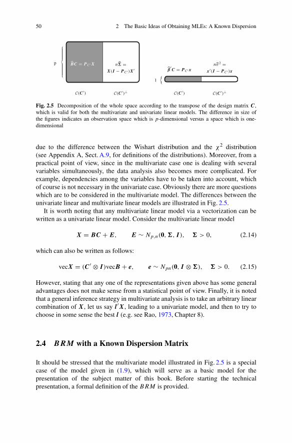
50 2 The Basic Ideas of Obtaining MLEs: A Known Dispersion
Fig. 2.5 Decomposition of the whole space according to the transpose of the design matrix C,which is valid for both the multivariate and univariate linear models. The difference in size ofthe figures indicates an observation space which is p-dimensional versus a space which is one-dimensional
due to the difference between the Wishart distribution and the χ2 distribution(see Appendix A, Sect. A.9, for definitions of the distributions). Moreover, from apractical point of view, since in the multivariate case one is dealing with severalvariables simultaneously, the data analysis also becomes more complicated. Forexample, dependencies among the variables have to be taken into account, whichof course is not necessary in the univariate case. Obviously there are more questionswhich are to be considered in the multivariate model. The differences between theunivariate linear and multivariate linear models are illustrated in Fig. 2.5.
It is worth noting that any multivariate linear model via a vectorization can bewritten as a univariate linear model. Consider the multivariate linear model
X = BC + E, E ∼ Np,n(0,�, I ), � > 0, (2.14)
which can also be written as follows:
vecX = (C′ ⊗ I )vecB + e, e ∼ Npn(0, I ⊗ �), � > 0. (2.15)
However, stating that any one of the representations given above has some generaladvantages does not make sense from a statistical point of view. Finally, it is notedthat a general inference strategy in multivariate analysis is to take an arbitrary linearcombination of X, let us say l′X, leading to a univariate model, and then to try tochoose in some sense the best l (e.g. see Rao, 1973, Chapter 8).
2.4 BRM with a Known Dispersion Matrix
It should be stressed that the multivariate model illustrated in Fig. 2.5 is a specialcase of the model given in (1.9), which will serve as a basic model for thepresentation of the subject matter of this book. Before starting the technicalpresentation, a formal definition of the BRM is provided.

2.4 BRM with a Known Dispersion Matrix 51
Definition 2.1 (BRM) Let X: p × n, A : p × q , q ≤ p, B: q × k, C: k × n,r(C) + p ≤ n and �: p × p be p.d. Then
X = ABC + E (2.16)
defines the BRM , where E ∼ Np,n(0,�, I ), A and C are known matrices, and B
and � are unknown parameter matrices.
The condition r(C) + p ≤ n is an estimability condition when � is unknown.However, for ease of presentation in this section, it is assumed that the dispersionmatrix � is known. The idea is to give a general overview and leave many detailsfor the subsequent sections.
For the likelihood, L(B), we have
L(B) ∝ |�|−n/2e−1/2tr{�−1(Xo−ABC)(Xo−ABC)′}.
From (2.16) it is seen that there exists a design matrix A which describes theexpectation of the rows of X (a within-individuals design matrix), as well as a designmatrix C which describes the mean of the columns of X (a between-individualsdesign matrix). It is known that if one pre- and post-multiplies a matrix, a bilineartransformation is performed. Thus, in a comparison of (1.7) and (2.16), instead of alinear model in (1.7), there is a bilinear one in (2.16). The previous techniques usedwhen Rn was decomposed into C(C′) � C(C′)⊥ are adopted; i.e. due to bilinearitythe tensor product Rp ⊗ Rn is decomposed as
(C(A) ⊗ C(C′)) � (C(A) ⊗ C(C′)⊥) � (C(A)⊥ ⊗ C(C′)) � (C(A)⊥ ⊗ C(C′)⊥).
Let the projections P A, = A(A′�−1A)−A′�−1 and P C ′ be as before (seeAppendix A, Sect. A.7). It appears that the likelihood can be decomposed as follows(omitting the proportionality constant (2π)−np/2):
L(B) ∝ |�|−n/2exp{−1/2tr{�−1PA,(Xo − ABC)(Xo − ABC)′P ′A,}}
×exp{−1/2tr{�−1(I − PA,)(Xo − ABC)(Xo − ABC)′(I − P ′A,)}},
since (I −P ′A,)�−1P A, = 0. Thus, a decomposition of Rp into two orthogonal
subspaces has been utilized. Continuing as in the linear case, i.e. using PC ′ andI − PC ′ , the following expression for the likelihood is obtained:
L(B) ∝ |�|−n/2exp{−1/2tr{�−1PA,(Xo − ABC)P C′(Xo − ABC)′P ′A,}}
×exp{−1/2tr{�−1P A,(Xo − ABC)(I − PC′)(Xo − ABC)′P ′A,}}
×exp{−1/2tr{�−1(I − PA,)(Xo − ABC)P C′(Xo − ABC)′(I − P ′A,)}}
×exp{−1/2tr{�−1(I − PA,)(Xo − ABC)(I − PC′)(Xo − ABC)′(I − P ′A,)}};

52 2 The Basic Ideas of Obtaining MLEs: A Known Dispersion
i.e. the likelihood consists of four factors. Utilizing (I − PA,)A = 0 and (I −P C ′)C′ = 0, this expression reduces to
L(B) ∝ |�|−n/2exp{−1/2tr{�−1PA,(Xo − ABC)PC ′(Xo − ABC)′P ′A,}}
×exp{−1/2tr{�−1P A,Xo(I − PC ′)X′oP
′A,}}
×exp{−1/2tr{�−1(I − P A,)XoPC ′X′o(I − P ′
A,)}}×exp{−1/2tr{�−1(I − P A,)Xo(I − PC ′)X′
o(I − P ′A,)}}, (2.17)
and only the first term involves the unknown parameter. Since � is supposed to beknown, the maximum of the likelihood occurs when
ABoC = P A,XoP C ′
= A(A′�−1A)−A′�−1XoC′(CC′)−C, (2.18)
because in (2.17) one term smaller than one cancels. If a vectorized form of themodel had been used, i.e.
vecX = (C′ ⊗ A)vecB + e, e ∼ Npn(0, I ⊗ �),
we would have obtained, applying standard linear models theory, the estimator givenin Sect. 2.2, which is a BLUE (best linear unbiased estimator). In the next section the“real” case when � is unknown will be considered. The decomposition of Rp ⊗Rn
when estimating the parameters is illustrated in Fig. 2.6.Note that C(A) means that the inner product is defined through �−1; i.e. take
any two vectors x and y from C(A) and then the inner product is defined by theoperation x′�−1y. When ABC is estimated, X is projected on the tensor spaceC(A) ⊗ C(C′). If C(A) is the whole space, P A = I , which for example takes
Fig. 2.6 Decomposition of the whole space according to the within-individuals and between-individuals designs, illustrating the mean and residual spaces in the BRM , and a comparison withthe multivariate linear model (MANOVA)

2.5 EBRMmB with a Known Dispersion Matrix 53
place when A: p × p is non-singular. Moreover, in Fig. 2.6, C(A)⊥ stands for thespace where any element, let us say u, satisfies u′�−1A = 0.
2.5 EBRMmB
with a Known Dispersion Matrix
In Sect. 1.5 two extensions of the BRM were presented, i.e. the EBRMmB and
EBRMmW , together with examples of the application of these models. In this section
the reader is introduced to the mathematics concerning the EBRMmB , with m = 3,
which will also be used later when studying the model without a known dispersionmatrix. Now (2.16) is formally generalized and the EBRMm
B is specified in detail.
Definition 2.2 (EBRMmB ) Let X: p × n, Ai : p × qi , qi ≤ p, B i : qi × ki , Ci :
ki × n, i = 1, 2, . . . ,m, r(C1) + p ≤ n, C(C′i ) ⊆ C(C′
i−1), i = 2, 3, . . . ,m, and�: p × p be p.d. Then
X =m∑
i=1
AiBiCi + E (2.19)
defines the EBRMmB , where E ∼ Np,n(0,�, I ), {Ai} and {Ci} are known matrices,
and {B i} and � are unknown parameter matrices.
In the present book it is usually assumed that m = 2, 3, and in this section �
is supposed to be known. In that case, r(C1) + p ≤ n, C(C′i ) ⊆ C(C′
i−1), i =2, 3, . . . ,m are not needed when estimating B i . However, since the results fromthis chapter will be utilized in the next chapter, it is assumed that C(C′
i ) ⊆ C(C′i−1),
i = 2, 3, . . . ,m, holds. Thus, the following model will be handled:
X = A1B1C1 + A2B2C2 + A3B3C3 + E, E ∼ Np,n(0,�, I ), (2.20)
where C(C′3) ⊆ C(C′
2) ⊆ C(C′1), Ai : p×qi , the parameter Bi : p×qi , is unknown,
Ci : ki ×n and the dispersion matrix � is supposed to be known. It has already beennoted in Sect. 1.5 that without the subspace condition on C(Ci ), we would havethe general “sum of profiles model” (a multivariate seemingly unrelated regression(SUR) model). Later (2.20) is studied when C(A3) ⊆ C(A2) ⊆ C(A1) replacesC(C′
3) ⊆ C(C′2) ⊆ C(C′
1), i.e. we have an EBRM3W . Since the model under the
assumption C(A3) ⊆ C(A2) ⊆ C(A1) through a reparametrization can be convertedto (2.20) and vice versa, i.e. EBRM3
B � EBRM3W , the models are in some sense
equivalent. However, because of non-linearity in estimators of mean parameters, thisdoes not imply that all the results for the models can easily be transferred from onemodel to the other.
From now on, under the nested subspace condition C(C′3) ⊆ C(C′
2) ⊆ C(C′1),
MLEs will be derived when � > 0 is known. The likelihood is proportional to
|�|−n/2exp{−1/2tr{�−1(Xo − E[X])()′}}, (2.21)

54 2 The Basic Ideas of Obtaining MLEs: A Known Dispersion
where E[X] = A1B1C1 + A2B2C2 + A3B3C3. A chain consisting of three linksof relatively straightforward calculations involving the trace function will start. Thecalculations will involve the following three basic quantities:
S1 = Xo(I − PC ′1)X′
o, (2.22)
P Ao1,
−1 = Ao1(A
o′1 �Ao
1)−Ao′
1 �, (2.23)
P A1, = A1(A′1�
−1A1)−A′
1�−1. (2.24)
For notational convenience Q1 = P Ao1,
−1 and P 1 = P A1, will be used. Note thatS1 is positive definite with probability 1 and both Q1 and P 1 are projectors whichare related, i.e. P 1 = I − Q′
1 (see Appendix B, Theorem B.11 (v)). Thus,
tr{�−1(Xo − E[X])()′} = tr{�−1S1} + tr{�−1(XoPC ′1− E[X])()′}
(because C(C′3) ⊆ C(C′
2) ⊆ C(C′1))
= tr{�−1S1} + tr{(XoP C ′1− E[X])′�−1(XoPC ′
1− E[X])}
(because tr(UV ) = tr(V U ))
= tr{�−1S1} + tr{(XoPC ′1− E[X])′�−1P 1(XoP C ′
1− E[X])}
+tr{(XoP C ′1− E[X])′Q1�
−1(XoP C ′1− E[X])}
(because Q1�−1 + �−1P 1 = �−1) (see Appendix B, Theorem B.11 (v))
≥ tr{�−1S1} + tr{(XoP C ′1− E[X])′Q1�
−1Q′1(XoP C ′
1− E[X])}
(because Q1�−1 = Q1�
−1Q′1)
= tr{�−1S1} + tr{�−1(Q′1XoP C ′
1− E[Q′
1X])()′} (2.25)
(because tr(UV ) = tr(V U )).
Note that E[Q′1X] = Q′
1A2B2C2 + Q′1A3B3C3; i.e. the parameter B1 has been
excluded (filtered) and thereby the number of parameters has been reduced. Equalityholds in (2.25) if and only if
A′1�
−1(XoPC ′1− A1B1C1 − A2B2C2 − A3B3C3) = 0, (2.26)

2.5 EBRMmB with a Known Dispersion Matrix 55
and this expression will later be used in order to determine B1. When continuing,the calculations which started with (2.22) will be repeated, but now using matriceswhich have been projected on C(A1)
⊥. Put
S2 = S1 + Q′1XoP C ′
1(I − P C ′
2)PC ′
1X′
oQ1, (2.27)
Q2 = P (Q′1A2)o,−1 = (Q′
1A2)o((Q′
1A2)o′�(Q′
1A2)o)−(Q′
1A2)o′�, (2.28)
P 2 = PQ′1A2,
= Q′1A2(A
′2Q1�
−1Q′1A2)
−A′2Q1�
−1 (2.29)
and then continuing from (2.25), as well as repeating the arguments used in (2.25),yields
tr{�−1S2} + tr{(Q′1XoPC ′
2− E[Q′
1X])′�−1(Q′1XoP C ′
2− E[Q′
1X])}= tr{�−1S2} + tr{(Q′
1XoP C ′2− E[Q′
1X])′�−1P 2(Q′1XoP C ′
2− E[Q′
1X])}+tr{(Q′
1XoP C ′2− E[Q′
1X])′Q2�−1(Q′
1XoP C ′2− E[Q′
1X])}≥ tr{�−1S2} + tr{(Q′
1XoP C ′2− E[Q′
1X])′Q2�−1Q′
2(Q′1XoPC ′
2− E[Q′
1X])}= tr{�−1S2} + tr{�−1(Q′
2Q′1XoPC ′
2− E[Q′
2Q′1X])()′}. (2.30)
Equality holds in (2.30) if and only if
A′2Q1�
−1(Q′1XoP C ′
2− Q′
1A2B2C2 − Q′1A3B3C3) = 0. (2.31)
Moreover, since in (2.30) E[Q′2Q
′1X] = Q′
2Q′1A3B3C3, we have in two steps
reduced the EBRM3B to a BRM . Let
S3 = S2 + Q′2Q
′1XoPC′
2(I − P C′
3)P C′
2X′
oQ1Q2, (2.32)
Q3 = P (Q′2Q′
1A3)o,−1 = (Q′2Q
′1A3)
o((Q′2Q
′1A3)
o′�(Q′
2Q′1A3)
o)−(Q′2Q
′1A3)
o′�,
(2.33)
P 3 = P Q′2Q
′1A3,
= Q′2Q
′1A3(A
′3Q1Q2�
−1Q′2Q
′1A3)
−A′3Q1Q2�
−1 (2.34)
and then advancing from (2.30) yields
tr{�−1S3} + tr{(Q′2Q
′1XoPC′
3− E[Q′
2Q′1X])′�−1(Q′
2Q′1XoPC′
3− E[Q′
2Q′1X])}
= tr{�−1S3}+tr{(Q′
2Q′1XoP C′
3− E[Q′
2Q′1X])′�−1P 3(Q
′2Q
′1XoPC′
3− E[Q′
2Q′1X])}
+tr{(Q′2Q
′1XoP C′
3− E[Q′
2Q′1X])′Q3�
−1(Q′2Q
′1XoPC′
3− E[Q′
2Q′1X])}

56 2 The Basic Ideas of Obtaining MLEs: A Known Dispersion
≥ tr{�−1S3} + tr{(Q′2Q
′1XoPC′
1)′Q3�
−1Q′3(Q
′2Q
′1XoPC′
1)}
= tr{�−1S3} + tr{�−1Q′3Q
′2Q
′1XoP C′
3X′
oQ1Q2Q3} (2.35)
with equality if and only if
A′3Q1Q2�
−1(Q′2Q
′1XoP C ′
3− Q′
2Q′1A3B3C3) = 0. (2.36)
It follows that the last line in (2.35) is independent of the parameters B i , i = 1, 2, 3,and if we can find estimators of Bi so that the lower bound is obtained, we havefound the MLEs.
From the above-presented chain of calculations, it follows from (2.26), (2.31)and (2.36) that three linear equations in three unknown parameters appear whichthen have to be solved. This means that if we can find solutions to these equations,the lower bound given in (2.35) can be attained. Thus we have to verify the existenceof a solution. From (2.36) it follows that
C(A′3Q1Q2�
−1Q′2Q
′1XoP C ′
3) ⊆ C(A′
3Q1Q2�−1Q′
2Q′1A3) = C(A′
3Q1Q2)
and thus there always exists a B3 (see Appendix B, Theorem B.10 (ii)). Moreover,for (2.31) there is a solution with respect to B2 if and only if
C(A′2Q1�
−1Q′1(XoP C ′
2− A3B3C3)) ⊆ C(A′
2Q1)
holds, which is always true, and finally (2.26) implies that a solution with respect toB3 exists if and only if
C(A1�−1(XoP C ′
1− A2B2C2 − A3B3C3)) ⊆ C(A1),
which also is trivially true. Thus there exists at least one solution. To estimate Bi ,i = 1, 2, 3, uniquely, we need conditions on C(Ai ), i = 1, 2, 3, which will beconsidered in Chap. 4. However, the general mean E[X] can always be uniquelyestimated:
E[X] = A1B10C1 + A2B20C2 + A3B30C3
= P 1XoP C ′1+ (I − P 1)(A2B20C2 + A3B30C3)
= P 1XoP C ′1+ Q′
1(A2B20C2 + A3B30C3)
= P 1XoP C ′1+ P 2Q
′1XoP C ′
2+ Q′
2Q′1A3B30C3
= P 1XoP C ′1+ P 2Q
′1XoP C ′
2+ P 3Q
′2Q
′1XoP C ′
3. (2.37)
In order to understand E[X], as well as the calculations leading to the finalexpression, it is of interest to note that calculations constitute projections ofobservations. Therefore, it is informative to know which spaces the observations

2.5 EBRMmB with a Known Dispersion Matrix 57
are projected onto. Moreover, since � is known, standard linear models theory (seeSect. 2.2) implies that E[X] should be expressed through a projector. Therefore,the projectors P 1, P 2 and P 3 will be exploited. To establish that P 1, P 2 and P 3are projectors, straightforward calculations show that each of the three matrices isidempotent. From (2.23) it follows that
C(P 1) = C(A1),
and using (2.29) and the projection theorem (Appendix B, Theorem B.11 (iv)) yields
C(P 2) = C(Q′1A2) = C(�Ao
1) ∩ (C(A1) + C(A2)) = C(A1)⊥ ∩ (C(A1 : A2)). (2.38)
Moreover, (2.34) implies
C(P 3) = C(Q′2Q
′1A3) = C(�(Q′
1A2)o) ∩ (C(Q′
1A2) + C(Q′1A3))
(because of the projection theorem, i.e. Appendix B, Theorem B.11 (iv))
= C(�(Q′1A2)
o) ∩ C(Q′1) ∩ (C(A1 : A2 : A3)
(because of the projection theorem, i.e. Appendix B, Theorem B.11 (iv), and (2.38))
= (C(A1) + C(�(A1 : A2)o)) ∩ C(�Ao
1) ∩ (C(A1 : A2 : A3)
= (C(A1) ∩ C(�Ao1) + C(�(A1 : A2)
o)) ∩ C(A1 : A2 : A3)
(through application of the modular identity, see Appendix B, Theorem B.3 (iv))
= C(�(A1 : A2)o) ∩ C(A1 : A2 : A3)
(because C(A1) ∩ C(�Ao1) = {0})
= C(A1 : A2)⊥ ∩ C(A1 : A2 : A3).
Note that these relations imply that P 2Q′1 = P 2 and P 3Q
′2Q
′1 = P 3, which means
that instead of (2.37),
E[X] = P 1XoP C ′1+ P 2XoP C ′
2+ P 3XoP C ′
3. (2.39)
Furthermore, when the inner product is defined via �, the projectors P 1, P 2 and P 3project onto orthogonal subspaces. Thus, there is enough information to generalizeFigs. 2.3 and 2.6 so that the EBRM3
B can also be described graphically, for exampleas in Fig. 2.7.

58 2 The Basic Ideas of Obtaining MLEs: A Known Dispersion
Fig. 2.7 Decomposition ofthe whole space according tothe within-individuals and thebetween-individuals designs,illustrating the mean andresidual spaces in theEBRM3
B : V1 = C(A1),V2 = C(A1 :A2) ∩ C(A1)
⊥,V3 = C(A1 : A2 :A3) ∩ C(A1 : A2)
⊥,V4 = C(A1 : A2 : A3)
⊥,W1 = C(C ′
3),W2 = C(C ′
2) ∩ C(C′3)
⊥,W3 = C(C ′
1) ∩ C(C′2)
⊥,W4 = C(C ′
1)⊥
Note that in Fig. 2.7 the so-called stairs structure is indicated, which is adistinctive feature of the EBRM•• .
The estimation procedure for obtaining E[X] will now be graphically illustrated.The fact is that if one understands the link between Fig. 2.7 and the derivation ofthe maximum likelihood estimators, more general models can be treated and, forexample, expressions for the EBRMm
B can be derived. Moreover, similar figureswill be used when working with the EBRM3
W . First it is noted that vec(E[X])belongs to the mean space
(V1 ⊗ (W1 �W1 �W1)) � (V2 ⊗ (W1 �W1)) � (V3 ⊗ W1);
the notation used here, including the definition of the subspaces, and the reasons forusing the expressions employed follow from Fig. 2.7.
The estimation of the parameters follows a three-step procedure with a finalupdating of expressions. The process is illustrated in Figs. 2.8 and 2.9. LetVi be as inFig. 2.7. In the first step of the estimation procedure the tensor space C(C′
1)⊗C(I )
is decomposed into two parts and the observation vector is projected on C(C′1)⊗V1
and C(C′1)⊗ (V2 �V3 �V4), via the projections (P C ′
1⊗P 1)xo and (P C ′
1⊗Q′
1)xo,where P 1 and Q1 are defined by (2.24) and (2.23), and xo = vecXo (see Fig. 2.8).The projection (P C ′
1⊗ P 1)xo is used for estimating B1 and one can, according
to (2.26), express B1o as a function of B2 and B3. Moreover, the second projectiondoes not include B1, which is essential. Relative to B1 the second projectiongenerates a residual space which is part of the total residual space (see Figs. 2.8and 2.9). This space will be utilized when estimating B2 and B3. In Fig. 2.8, P1symbolizes the projection.
In the second step the ideas from the first step are repeated and C(C′2) ⊗ (V2 �
V3�V4) is decomposed into two parts, C(C′2)⊗V2 and C(C′
2)⊗(V3�V4). Therefore,(P C ′
2⊗P 2)(PC ′
1⊗Q′
1)xo and (P C ′2⊗Q′
2)(P C ′1⊗Q′
1)xo will be utilized. However,

2.5 EBRMmB with a Known Dispersion Matrix 59
Fig. 2.8 Illustration of the various steps in the maximum likelihood estimation procedure. Fordetails, the reader is referred to the text
Fig. 2.9 Illustration of the steps when obtaining maximum likelihood estimators. For the notationsee Fig. 2.7 and the text
(P C ′2⊗P 2)(P C ′
1⊗Q′
1) = P C ′2⊗P 2 and (P C ′
2⊗Q′
2)(PC ′1⊗Q′
1) = P C ′2⊗Q′
2Q′1.
According to (2.31) and P C ′2
⊗ P 2, B2o can be expressed as a function of B3.Moreover, the projection on the new residual space is in Fig. 2.8 indicated by P2.
In the third step C(C′3)⊗(V2�V3�V4) is also decomposed into two parts and the
part which is obtained from the projection (PC ′3⊗ P 3)xo is used to estimate B3.
The explicit expression for B3o is obtained from (2.36). Since there are no moreunknown parameters involved in B3o, all the estimators can be found via a finalbackwards updating; i.e. B3o is used in (2.31) in order to find B2o and then B3o andB2o are used in (2.26).
So far we have only considered how to estimate the parameters of the model. Thestatistical paradigm, however, demands that methods for validating the EBRMm
B
should be developed. Many natural methods are based on the exploration of residual

60 2 The Basic Ideas of Obtaining MLEs: A Known Dispersion
spaces; i.e. we have to consider the tensor space (C(C′1⊗A1)+C(C′
2⊗A2)+C(C′3⊗
A3))⊥, which equals
(C(C′1 ⊗ A1) + C(C′
2 ⊗ A2) + C(C′3 ⊗ A3))
⊥
= C(C′3) ⊗ C(A1 : A2 : A3)
⊥ � C(C′3)
⊥ ∩ C(C′2) ⊗ C(A1 : A2)
⊥
� C(C′2)
⊥ ∩ C(C′1) ⊗ C(A1)
⊥ � C(C′1)
⊥ ⊗ Rp. (2.40)
Thus, residuals are introduced which are projections on the subspaces introducedin (2.40), i.e.
R1 = X(I − P C ′1), R2 = Q′
1XP C ′1,
R3 = Q′2Q
′1XPC ′
2, R4 = Q′
3Q′2Q
′1XP C ′
3.
Indeed, a finer division of the subspaces can be performed and this is illustrated viathe BRM , where
R11 = PA,X(I − PC ′), R21 = (I − P A,)X(I − P C ′), (2.41)
R2 = (I − P A,)XP C ′ . (2.42)
All these residuals are presented in Fig. 2.10. However, any treatment and utilizationof the residuals are postponed until the models are considered under the assumptionof an unknown �.
The following is worth noting. Suppose that in the BRM there are bilinearrestrictions on the mean parameters, i.e.
E[X] = ABC, FBG = 0,
where F and G are known matrices. Because FBG = 0 forms a linear system ofequations, the restriction FBG = 0 can be reformulated as follows (see AppendixB, Theorem B.10 (i)):
B = (F ′)o�1 + F ′�2Go′,
Fig. 2.10 Illustration of fourresidual spaces in theEBRM3
B and the threeresidual spaces in the BRM .For the notation see Fig. 2.7

2.5 EBRMmB with a Known Dispersion Matrix 61
(a) (b) (c)
Fig. 2.11 In (a), a BRM without restrictions is shown, in (b), the area where FBG = 0 may havean effect is illustrated and in (c), FBG = 0 holds, leading to a stairs structure, i.e. an EBRM2
B .Furthermore, V1 = C(A(F ′)o), V2 = C(A) ∩ C(A(F ′)o)⊥, V3 = C(A)⊥, W1 = C(C ′Go),W2 = C(C ′) ∩ C(C ′Go)⊥ and W3 = C(C ′)⊥
where �1 and �2 are new parameters. Thus the BRM with bilinear restrictionsturns into an EBRM2
B . This is illustrated in Fig. 2.11. Later in Chaps. 3 and 7a complete theory is presented concerning how to estimate parameters and testhypotheses when bilinear restrictions exist.
This section is ended by briefly considering residuals for the liming datapresented in Example 1.5.
Example 2.1 In Example 1.5, liming data for 20 Swedish lakes were presented. ABRM with � = I 3 and A, given in Example 1.5, was applied and led to
Bo =(
7.09 7.03−0.03 −0.04
)
. (2.43)
The residuals R11, R21 and R2 in Fig. 2.10 were calculated according to (2.41)and (2.42), and are presented in Table 2.1. Now the problem is to interpret theresiduals and decide if there are any extreme residuals. This can be accomplished inmany ways. It is, however, crucial that we derive the distributions for the residuals(e.g. for the largest or the smallest residual). A detailed handling of the residuals willbe provided in Chap. 6. Moreover, it should be noted that if, for example, the valuefor Lake 1, depth 0.5 m is changed from 6.72 to 10, this will affect the residualsin Region 1, whereas the residuals in Region 2 will be unaffected. The residual forLake 1, depth 0.5 m changes from −0.3 to 2.1. Other changes also appear, but arenot very pronounced. If the values for Lake 1, depth 5 and 10 m are also altered,supposed to equal 10, the three residuals R11 for Lake 1 equal 2.6, 2.7 and 2.8,respectively, are much larger than the other residuals. Thus, it has been demonstratedthat outstanding observations can be identified via the residuals. ��

62 2 The Basic Ideas of Obtaining MLEs: A Known Dispersion
Table 2.1 Residuals for the liming data presented in Example 1.5 where in the model � = I 3
Lake R11 R21 × 10−3 R2 × 10−2 Lake R11 R21 × 10−3 R2 × 10−2
1 −0.3 5 −2 11 0.2 109 −2
1 −0.3 −9 3 11 0.1 −207 4
1 −0.3 4 −2 11 0.1 98 −2
2 −0.3 0.9 −2 12 −0.1 −15 −2
2 −0.2 −2 3 12 0.0 28 4
2 −0.0 0.8 −2 12 0.1 −13 −2
3 0.1 7 −2 13 0.3 −52 −2
3 0.2 −13 3 13 0.4 100 4
3 0.3 6 −2 13 0.6 −47 −2
4 0.1 −8 −2 14 −0.1 41 −2
4 0.2 15 3 14 −0.2 77 4
4 0.3 −7 −2 14 −0.4 −37 −2
5 −0.1 36 −2 15 −0.3 4 −2
5 −0.2 −70 3 15 −0.4 −7 4
5 −0.3 32 −2 15 −0.4 3 −2
6 0.2 20 −2 16 −0.1 7 −2
6 0.1 −37 3 16 −0.2 −14 4
6 0.0 18 −2 16 −0.4 6 −2
7 −0.2 −7 −2 17 −0.0 15 −2
7 −0.2 12 3 17 −0.2 −28 4
7 −0.3 −6 −2 17 0.4 13 2
8 0.1 −51 −2 18 −0.1 −56 −2
8 0.1 97 3 18 0.1 105 4
8 0.1 −46 −2 18 0.2 −50 −2
9 0.2 5 −2 19 0.0 22 −2
9 0.1 −9 3 19 0.1 −42 4
9 −0.0 4 −2 19 0.2 20 −2
10 0.2 7 −2 20 0.2 7 −2
10 0.2 12 3 20 0.3 −14 4
10 0.3 −6 −2 20 0.5 6 −2
2.6 EBRMmW
with a Known Dispersion Matrix
Here the estimators for the EBRM3W when � is known are derived and compared
with the estimators for the EBRM3B , which were obtained in the previous section.
For completeness, the definition of the model under consideration is given below.
Definition 2.3 (EBRMmW ) Let X: p×n, Ai : p×qi , qi ≤ p, B i : qi×ki , Ci : ki×n,
i = 1, 2, . . . ,m, r(C′1 : C′
2 : C′3) + p ≤ n, C(Ai ) ⊆ C(Ai−1), i = 2, 3, . . . ,m, and

2.6 EBRMmW with a Known Dispersion Matrix 63
�: p × p be p.d. Then
X =m∑
i=1
AiBiCi + E (2.44)
defines the EBRMmW , where E ∼ Np,n(0,�, I ), {Ai} and {Ci} are known matrices,
and {B i} and � are unknown parameter matrices.
When estimating the parameters of the EBRM3B , a chain of straightforwardly
performed calculations was presented. Now, in order to estimate the parameters inthe EBRM3
W , a between-individuals subspace decomposition is utilized and it isnoted that (use Appendix B, Theorem B.3 (iii))
Rn = C(C′1) � C(C′
1)⊥ ∩ C(C′
1 : C′2) � C(C′
1 : C′2)
⊥ ∩ C(C′1 : C′
2 : C′3)
� C(C′1 : C′
2 : C′3)
⊥.
Let P i , i = 1, 2, 3, 4, be orthogonal projections on these spaces, i.e.
P 1 = PC ′1, P 2 = P Q1C
′2, P 3 = PQ2Q1C
′3, P 4 = P (C ′
1:C ′2:C ′
3)o , (2.45)
where
Q1 = P (C ′1)
o , Q2 = P (C ′1:C ′
2)o .
The likelihood up to proportionality is stated in (2.21) and from there it follows thatone should consider
tr{�−1(Xo − E[X])(Xo − E[X])′} =4
∑
i=1
tr{�−1(Xo − E[X])P i (Xo − E[X])′},
where one has utilized the fact that P 1 + P 2 + P 3 + P 4 = I , since∑4
i=1 P i is aprojector on the whole space. Because of the stairs structure, the within-individualsspace, i.e. Rp, is split. Hence,
tr{�−1(Xo − E[X])(Xo − E[X])′} = tr{�−1(Xo − E[X])P 4(Xo − E[X])′} (2.46)
+3
∑
i=1
tr{�−1P Ai,(Xo − E[X])P i (Xo − E[X])′P ′Ai,
} (2.47)
+3
∑
i=1
tr{�−1P ′Ao
i ,−1 (Xo − E[X])P i (Xo − E[X])′P Ao
i ,−1}. (2.48)
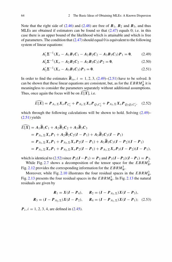
64 2 The Basic Ideas of Obtaining MLEs: A Known Dispersion
Note that the right side of (2.46) and (2.48) are free of B1, B2 and B3, and thusMLEs are obtained if estimators can be found so that (2.47) equals 0; i.e. in thiscase there is an upper bound of the likelihood which is attainable and which is freeof parameters. The condition that (2.47) should equal 0 is equivalent to the followingsystem of linear equations:
A′1�
−1(Xo − A1B1C1 − A2B2C2 − A3B3C3)P 1 = 0, (2.49)
A′2�
−1(Xo − A2B2C2 − A3B3C3)P 2 = 0, (2.50)
A′3�
−1(Xo − A3B3C3)P 3 = 0. (2.51)
In order to find the estimates Bio, i = 1, 2, 3, (2.49)–(2.51) have to be solved. Itcan be shown that these linear equations are consistent, but, as for the EBRM3
B it ismeaningless to consider the parameters separately without additional assumptions.Thus, once again the focus will be on E[X], i.e.
E[X] = P A1,XoP C ′1+ P A2,XoP Q1C
′2+ PA3,XoP Q2Q1C
′3, (2.52)
which through the following calculations will be shown to hold. Solving (2.49)–(2.51) yields
E[X] = A1B1C1 + A2B2C2 + A3B3C3
= PA1,XoP 1 + A2B2C2(I − P 1) + A3B3C3(I − P 1)
= PA1,XoP 1 + PA2,XoP 2(I − P 1) + A3B3C3(I − P 2)(I − P 1)
= PA1,XoP 1 + PA2,XoP 2(I − P 1) + PA3,XoP 3(I − P 2)(I − P 1),
which is identical to (2.52) since P 2(I −P 1) = P 2 and P 3(I −P 2)(I −P 1) = P 3.While Fig. 2.7 shows a decomposition of the tensor space for the EBRM3
B ,Fig. 2.12 provides the corresponding information for the EBRM3
W .Moreover, while Fig. 2.10 illustrates the four residual spaces in the EBRM3
B ,Fig. 2.13 presents the four residual spaces in the EBRM3
W . In Fig. 2.13 the naturalresiduals are given by
R1 = X(I − P 4), R2 = (I − P A3,)X(I − P 3),
R3 = (I − P A2,)X(I − P 2), R4 = (I − P A1,)X(I − P 1); (2.53)
P i , i = 1, 2, 3, 4, are defined in (2.45).

2.6 EBRMmW with a Known Dispersion Matrix 65
Fig. 2.12 Decomposition of the whole space according to the within-individuals and the between-individuals designs, illustrating the mean and residual spaces in the EBRM3
W : V1 = C(A3),V2 = C(A2) ∩ C(A3)
⊥, V3 = C(A1) ∩ C(A2)⊥, V4 = C(A1)
⊥, W1 = C(C ′1), W2 =
C(C ′1 : C′
2) ∩ C(C ′1)
⊥, W3 = C(C′1 : C′
2 : C ′3) ∩ C(C ′
1 : C ′2)
⊥, W4 = C(C ′1 : C ′
2 : C′3)
⊥. The
estimator E[X] is presented in (2.52)
Fig. 2.13 Illustration of the four residual spaces in the EBRM3W . For the notation see Fig. 2.12
Problems
1 Give examples, i.e. specify appropriate matrices, of a weakly singular and astrongly singular Gauss-Markov model.
2 Let
x′ = β ′C + ε, ε ∼ Nn(0, σ 2V ), V p.s.d.
and suppose that β ′L = 0, for some known matrix L. Estimate the parameters β
and σ 2.

66 2 The Basic Ideas of Obtaining MLEs: A Known Dispersion
3 Suppose that the model is identical to the one in (2.44) with m = 2 and known�. Estimate B1 and give conditions on K and L so that KB1L does not depend onany choice of g-inverses.
4 In (2.20) let A3 = 0. Find, for given �, maximum estimators of B1, B2 anddetermine
X = A1B1C1 + A2B2C2.
Moreover, show that E[X] = A1B1C1 + A2B2C2.
5 Let the model be given by (2.20), but suppose that the nested subspace conditionC(C′
3) ⊆ C(C′2) ⊆ C(C′
1) does not hold. Derive expressions for Bi , i = 1, 2, 3.
6 For each task presented below create three matrices: A1, A2 and A3.
(i) Create the matrices such that C(Ai ) is orthogonal to C(Aj ), i �= j .(ii) Create the matrices such that C(Ai ) is disjoint with C(Aj ), i �= j , but not
orthogonal.(iii) Create matrices such that C(A1) ∩ C(A2) = {0}, C(A1) ∩ C(A3) = {0}, but
C(A1) ∩ C(A2 : A3) �= {0}.7 Show that |�| is proportional to
∫
exp{−1/2tr{�−1yy ′}}dy,
where � is a dispersion matrix of full rank.
8 Show that |S + V V ′| ≥ |S|, where S is p.d. and V is any matrix of a proper size.
9 Let Ri , i = 1, 2, 3, be given by (2.53). Are these residuals mutually indepen-dently distributed? Why/why not?
10 Solve (2.49)–(2.51).
Literature
In this chapter the dispersion matrix was supposed to be known, and therefore wehave the obvious connections between the BRM , the EBRMm• and univariate linearmodels, generally speaking the Gauss-Markov model. Therefore, it is appropriatehere to provide some background references on univariate linear models. Beforecommencing, from a practical point of view it is worth noting that analysis ofvariance, regression analysis and covariance analysis can all be treated in thesame fashion within linear models theory. However, for each of these topics,of course, special problems and ideas have been dealt with and exploited, for

2.6 EBRMmW with a Known Dispersion Matrix 67
example balancedness, multiple testing problems, variable selection and a hugerange of methods for performing model validation, including the topic of influentialobservations (see Chap. 8 for references). A general ultimate goal has been todevelop corresponding results for the BRM and its extensions, but this has onlybeen partly fulfilled.
In his classical book entitled “The Design and Analysis of Experiments”,Kempthorne (1952) presented, among other things, general linear univariate modelswith the help of matrices (see also Hinkelmann and Kempthorne, 2005, 2008). Themain topic of Kempthorne’s book was analysis of variance methods, which weretreated in great detail, and even today this book is still highly useful. It constitutes abasis for a solid handling of models connected to least squares. The development ofmethods for handling models via least squares was to a large extent complete in the1960s. Some other well-known books on linear models and their theory have beenpresented by Scheffé (1959), Graybill (1961, 1976), Seber (1966), Searle (1971,1987) and Rao (1973). In contrast to Kempthorne’s work, the authors who cameafter him (in particular Rao) started to use generalized inverses (g-inverses) insteadof performing reparametrizations, in order to handle the rank deficiencies of thedesign matrix in the general linear model. In the 1960s a large amount of researchactivities on g-inverses started, although the concept is much older. Today manybooks are available which specialize in g-inverses, for example, the classical workby Rao and Mitra (1971) or the newer book by Ben-Israel and Greville (2003),which among other things includes many references connected to g-inverses (notethat the first edition of the book by Ben-Israel and Greville appeared in the 1970s).In parallel with all the above-mentioned publications, interesting work on linearmodels (slightly more abstract in nature and based on linear spaces and a coordinate-free approach) was performed by Kruskal (1961), Drygas (1970), Eaton (1970) (seeEaton, 2007, for some notes on Kruskal’s work), Stone (1977, 1987) and Wong(1993), among others. Among the more recently published works on linear modelsis the book by Sengupta and Jammalamadaka (2003), who present the topic in aclear and interesting way.
After the basic theory on linear models had been established the academicchallenge was then to develop methods for handling a general linear model with aknown singular dispersion matrix. Under the assumption of a singular dispersionmatrix, there exist random variables which equal a constant with probability 1,which is indeed quite special. This leads to some philosophical concerns (seeBaksalary et al., 1992). With regard to non-singular dispersion Aitken (1936) hadalready presented work on estimation and least squares, i.e. had derived the bestlinear unbiased estimator of the mean parameter. There exists a huge volume ofliterature on the singular Gauss-Markov model, for example Zyskind and Martin(1969), Rao (1973, Chapter 4i), Alalouf (1978), Baksalary and Kala (1979, 1981),Nordström (1985), Tian et al. (2008) and Baksalary and Trenkler (2011). Inparticular we refer to Nordström, because he divided the singular Gauss-Markovmodel into two cases, i.e. the weakly singular and the strongly singular Gauss-Markov model, and to Baksalary & Trenkler for a number of recent references.

68 2 The Basic Ideas of Obtaining MLEs: A Known Dispersion
Concerning the BRM , it is of interest to discuss weighted versus unweightedestimators of the mean parameters. This topic has a long history within the Gauss-Markov model framework (see Puntanen et al., 2011, Chapter 10; Haslett et al.,2014). For a complete set of references on the topic up to 1989, one should consultPuntanen and Styan (1989).
It should be noted that there are articles which treat in detail the EBRMm• (andthe BRM) with almost-known dispersion matrices (proportional to an unknownconstant), i.e. a Gauss-Markov model where the overall design matrix is a sum ofKronecker products of matrices and thus the corresponding linear space is a tensorproduct. Examples of such articles are those written by Tian and Takane (2007,2009), Beganu (2009), Song (2011) and Song and Wang (2014), who consideredbest linear unbiased estimators (see also Zhang and Zhu, 2000; Xu and Wang, 2011).Also relevant for this book are the results and ideas of Hu (2010), who proposed,by first assuming a known dispersion matrix, a two-stage estimator of the meanparameters. Admissibility of linear estimators for the BRM with known correlation,under some specific restrictions, was obtained by Zhang and Gui (2008) and Zhanget al. (2009, 2011).
References
Aitken, A. C. (1936). On least squares and linear combinations of observations. Proceedings of theRoyal Society of Edinburgh, Section A, 55, 42–48.
Alalouf, I. S. (1978). An explicit treatment of the general linear model with singular covariancematrix. Sankhya, Series B, 40, 65–73.
Baksalary, J. K., & Kala, R. (1979). Best linear unbiased estimation in the restricted general linearmodel. Mathematische Operationsforschung und Statistik, Series Statistics, 10, 27–35.
Baksalary, J. K., & Kala, R. (1981). Linear transformations preserving best linear unbiasedestimators in a general Gauss-Markoff model. Annals of Statistics, 9, 913–916.
Baksalary, J. K., Rao, C. R., & Markiewicz, A. (1992). A study of the influence of the “naturalrestrictions” on estimation problems in the singular Gauss-Markov model. The Journal ofStatistical Planning and Inference, 31, 335–351.
Baksalary, O. M., & Trenkler, G. (2011). Between OLSE and BLUE. Australian and New ZealandJournal of Statistics, 53, 289–303.
Beganu, G. (2009). Some properties of the best linear unbiased estimators in multivariate growthcurve models. RACSAM - Revista de la Real Academia de Ciencias Exactas, Fisicas yNaturales. Serie A. Matematicas, 103, 161–166.
Ben-Israel, A., & Greville, T. N. E. (2003). Generalized inverses. Theory and applications. CMSbooks in mathematics/Ouvrages de Mathématiques de la SMC (Vol. 15, 2nd ed.). New York:Springer.
Drygas, H. (1970). The coordinate-free approach to Gauss-Markov estimation. Lecture notes inoperations research and mathematical systems (Vol. 40). New York: Springer.
Eaton, M. L. (1970). Gauss-Markov estimation for multivariate linear models: A coordinate freeapproach. Annals of Mathematical Statistics, 41, 528–538.
Eaton, M. L. (2007). William H. Kruskal and the development of coordinate-free methods.Statistical Science, 22, 264–265.
Graybill, F. A. (1961). An introduction to linear statistical models. McGraw-Hill series inprobability and statistics (Vol. I). New York: McGraw-Hill.

References 69
Graybill, F. A. (1976). Theory and application of the linear model. North Scituate: Duxbury Press.Haslett, S. J., Isotalo, J., Liu, Y., & Puntanen, S. (2014). Equalities between OLSE, BLUE and
BLUP in the linear model. Statistical Papers, 55, 543–561.Hinkelmann, K., & Kempthorne, O. (2005). Design and analysis of experiments. Vol. 2. Advanced
experimental design. Wiley series in probability and statistics. Hoboken: Wiley.Hinkelmann, K., & Kempthorne, O. (2008). Design and analysis of experiments. Vol. 1. Intro-
duction to experimental design. Wiley series in probability and statistics (2nd ed.). Hoboken:Wiley.
Hu, J. (2010). Properties of the explicit estimators in the extended growth curve model. Statistics:A Journal of Theoretical and Applied Statistics, 44, 477–492.
Kempthorne, O. (1952). The design and analysis of experiments. New York/London:Wiley/Chapman & Hall.
Kollo, T., & von Rosen, D. (2005). Advanced multivariate statistics with matrices. Mathematicsand its applications (Vol. 579). Dordrecht: Springer.
Kruskal, W. (1961). The coordinate-free approach to Gauss-Markov estimation, and its applicationto missing and extra observations. In Proceedings of the Fourth Berkeley Symposium on Math-ematical Statistics and Probability (Vol. I, pp. 435–451). Berkeley: University of CaliforniaPress.
Nordström, K. (1985). On a decomposition of the singular Gauss-Markov model. In: Linearstatistical inference (Poznan, 1984). Lecture notes in statistics (Vol. 35, pp. 231–245). Berlin:Springer.
Puntanen, S., & Styan, G. P. H. (1989). The equality of the ordinary least squares estimator andthe best linear unbiased estimator. With comments by Oscar Kempthorne and Shayle R. Searleand a reply by the authors. The American Statistician, 43, 153–164.
Puntanen, S., Styan, G. P. H., & Isotalo, J. (2011). Matrix tricks for linear statistical models. Ourpersonal top twenty. Heidelberg: Springer.
Rao, C. R. (1973). Linear statistical inference and its applications. Wiley series in probability andmathematical statistics (2nd ed.). New York: Wiley.
Rao, C. R., & Mitra, S. K. (1971). Generalized inverse of matrices and its applications. New York:Wiley.
Scheffé, H. (1959). The analysis of variance. New York/London: Wiley/Chapman & Hall.Searle, S. R. (1971). Linear models. New York: Wiley.Searle, S. R. (1987). Linear models for unbalanced data. Wiley series in probability and
mathematical statistics: Applied probability and statistics. New York: Wiley.Seber, G. A. F. (1966). The linear hypothesis: A general theory. Griffin’s statistical monographs &
courses (Vol. 19). London: Charles Griffin.Sengupta, D., & Jammalamadaka, S. R. (2003). Linear models. An integrated approach. Series on
multivariate analysis. (Vol. 6). River Edge: World Scientific.Song, G. J. (2011). On the best linear unbiased estimator and the linear sufficiency of a general
growth curve model. The Journal of Statistical Planning and Inference, 141, 2700–2710.Song, G. J., & Wang, Q. W. (2014). On the weighted least-squares, the ordinary least-squares and
the best linear unbiased estimators under a restricted growth curve model. Statistical Papers,55, 375–392.
Stone, M. (1977). A unified approach to coordinate-free multivariate analysis. Annals of theInstitute of Statistical Mathematics, 29, 43–57.
Stone, M. (1987). Coordinate-free multivariable statistics. An illustrated geometric progressionfrom Halmos to Gauss and Bayes. Oxford statistical science series (Vol. 2). New York: TheClarendon Press/Oxford University Press.
Tian, Y., Beisiegel, M., Dagenais, E., & Haines, C. (2008). On the natural restrictions in the singularGauss-Markov model. Statistical Papers, 49, 553–564.
Tian, Y., & Takane, Y. (2007). Some algebraic and statistical properties of WLSEs under a generalgrowth curve model. Electronic Journal of Linear Algebra, 16, 187–203.

70 2 The Basic Ideas of Obtaining MLEs: A Known Dispersion
Tian, Y., & Takane, Y. (2009). On consistency, natural restrictions and estimability under classicaland extended growth curve models. The Journal of Statistical Planning and Inference, 139,2445–2458.
Wong, C. S. (1993). Linear models in a general parametric form. Sankhya , Series A, 55, 130–149.Xu, L.-W., & Wang, S.-G. (2011). Linear sufficiency in a general growth curve model. Linear
Algebra and Its Applications, 434, 593–604.Zhang, B. X., & Zhu, X. H. (2000). Gauss-Markov and weighted least-squares estimation under a
general growth curve model. Linear Algebra and Its Applications, 321, 387–398.Zhang, S., Fang, Z., Qin, H., & Han, L. (2011). Characterization of admissible linear estimators in
the growth curve model with respect to inequality constraints. Journal of the Korean StatisticalSociety, 40, 173–179.
Zhang, S., & Gui, W. (2008). Admissibility of linear estimators in a growth curve model subjectto an incomplete ellipsoidal restriction. Acta Mathematica Scientia. Series B. English Edition,28, 194–200.
Zhang, S., Gui, W., & Liu, G. (2009). Characterization of admissible linear estimators in thegeneral growth curve model with respect to an incomplete ellipsoidal restriction. LinearAlgebra and Its Applications, 431, 120–131.
Zyskind, G., & Martin, F. B. (1969). On best linear estimation and general Gauss-Markov theoremin linear models with arbitrary nonnegative covariance structure. SIAM Journal on AppliedMathematics, 17, 1190–1202.

Chapter 3The Basic Ideas of Obtaining MLEs:Unknown Dispersion
3.1 Introduction
In this chapter, the maximum likelihood estimators of all the parameters in theBRM , EBRM3
W and EBRM3B are derived when the dispersion is supposed to
be unknown; i.e. when following the statistical paradigm, it is supposed that theexperiment has been designed and accomplished, and now it is time to estimatethe parameters of the model. Only the estimators are obtained, while statisticalproperties such as their distributions are left to subsequent chapters. The subjectmatter of this chapter is essential for the book and it is worthwhile devoting sometime to reflection on the derivations and results.
3.2 BRM and Its MLEs
Let
X = ABC + E, E ∼ Np,n(0,�, I ), � > 0, (3.1)
where all matrices are specified in Definition 2.1. From general maximum likelihoodtheory we know that estimators are consistent. This means that the MLE of �,should converge to � and, therefore, intuitively, the estimators of B with a knownor estimated � should be of a similar form. Let us restate the appropriate part ofFig. 2.6 as Fig. 3.1 which will serve as a basis for understanding how subspaces areconnected to the MLEs.
© Springer International Publishing AG, part of Springer Nature 2018D. von Rosen, Bilinear Regression Analysis, Lecture Notes in Statistics 220,https://doi.org/10.1007/978-3-319-78784-8_3
71
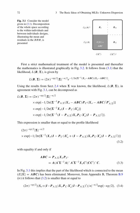
72 3 The Basic Ideas of Obtaining MLEs: Unknown Dispersion
Fig. 3.1 Consider the modelgiven in (3.1). Decompositionof the whole space accordingto the within-individuals andbetween-individuals designs,illustrating the mean andresiduals in the BRM , ispresented
First a strict mathematical treatment of the model is presented and thereafterthe mathematics is illustrated graphically in Fig. 3.2. It follows from (3.1) that thelikelihood, L(B,�), is given by
L(B,�) = (2π)−np/2|�|−n/2e−1/2tr{�−1(Xo−ABC)(Xo−ABC)′}.
Using the results from Sect. 2.4 when � was known, the likelihood, L(B,�), inagreement with Fig. 3.1, can be decomposed as
L(B,�) = (2π)−np/2|�|−n/2
× exp{−1/2tr{�−1P A,(Xo − ABC)PC ′(Xo − ABC)′P ′A,}}
× exp{−1/2tr{�−1Xo(I − P C ′)X′o}}
× exp{−1/2tr{�−1(I − P A,)XoPC ′X′o(I − P A,)′}}.
This expression is smaller than or equal to the profile likelihood
(2π)−np/2|�|−n/2
× exp{−1/2tr{�−1(Xo(I − P C ′)X′o + (I − P A,)XoP C ′X′
o(I − P A,)′)}}(3.2)
with equality if and only if
ABC = PA,XoP C ′
= A(A′�−1A)−A′�−1XoC′(CC′)−C. (3.3)
In Fig. 3.1 this implies that the part of the likelihood which is connected to the mean(E[X] = ABC) has been eliminated. Moreover, from Appendix B, Theorem B.9(iv) it follows that (3.2) is smaller than or equal to
(2π)−np/2|(So+(I−PA,)XoP C ′X′o(I−PA,)′)/n|−n/2exp{−np/2}, (3.4)

3.2 BRM and Its MLEs 73
where So = Xo(I − P C ′)X′o, which is obtained if
n� = So + (I − P A,)XoP C ′X′o(I − P A,)′ (3.5)
is inserted in (3.2). Since the right-hand side of (3.5) equals (Xo−ABC)()′, there isno problem applying Theorem B.9 (iv) in Appendix B. It is less clear if this theoremcan be applied for optimization purposes, if instead of B, we have a function in �;i.e. B(�), which sometimes appears.
Using (2.41) and (2.42), it follows from (3.5) that n� = R11R′11 + R21R
′21 +
R2R′2, among other things showing the whole tensor space Rn ⊗Rp to be included
in the estimation process. Both Eqs. (3.3) and (3.5) are complicated functionsin �, but fortunately the only requirement for finding explicit MLEs are a fewstraightforward calculations. Pre-multiplying (3.5) by A′�−1 yields
nA′ = A′�−1So,
and thus under the assumption that S−1o exists
A′�−1 = nA′S−1o . (3.6)
This means that A′�−1 has been estimated, which is exactly what is neededin (3.3) and (3.5) because P A, is used, and now it is known that P A, = P A,So .It follows that the upper bound in (3.4) does not depend on any unknown parameterand is obtained by inserting the estimates given in (3.3) and (3.5), in the likelihood,
which thus yields MLEs. Moreover, A′�−1 = A′�
−1. We may summarize our
finding as follows. Out of all the relations, the relation shown in (3.6) is the mostimportant one because it implies:
1. the finding of an upper bound of the likelihood function;2. the finding of MLEs;3. establishment of the relation P A, = P A,S .
In particular, implication (3) tells us that there is no great difference betweenobtaining MLEs when � is known and obtaining them when � is unknown, sinceall the estimators, including the estimators of the residuals R11, R21 and R2 aresimilar, i.e. the projection operators used in the estimation process project on thesame spaces.
In the next theorem the above results are summarized and the MLEs of B and �
are explicitly presented.
Theorem 3.1 For the BRM given in Definition 2.1 and with S = X(I − P C ′)X′supposed to be p.d., with n − r(C) ≥ p, the MLEs are given by
ABC = A(A′S−1A)−A′S−1XC′(CC′)−C,
n� = S + (I − A(A′S−1A)−A′S−1)XC′(CC′)−CX′(I − S−1A(A′S−1A)−A′).

74 3 The Basic Ideas of Obtaining MLEs: Unknown Dispersion
The assumption that S is p.d. holds with probability 1, if n − r(C) ≥ p. Moreover,� is always unique, i.e. does not depend on any choice of g-inverse.
Corollary 3.1 Let B satisfy the relation ABC given in Theorem 3.1. Then
B = (A′S−1A)−A′S−1XC ′(CC′)− + (A′)oZ1 + A′Z2Co′,
where Z1 and Z2 are arbitrary matrices.If the estimability conditions C(K ′) ⊆ C(A′) and C(L) ⊆ C(C) are fulfilled,
then
KBL = K(A′S−1A)−A′S−1XC′(CC′)−L,
which is independent of any choice of g-inverse, i.e. is unique.If ρ(A) = q and ρ(C) = k, then
B = (A′S−1A)−1A′S−1XC′(CC′)−1.
It is questionable whether B under non-estimability should be called an estimator,because Z1 and Z2 are both unknown and unrestricted. For this reason B, in thiscase, is definitely not a very useful quantity.
Corollary 3.2 If A = I , then
BC = XC′(CC′)−C,
n� = S.
In Corollary 3.2 the MLEs for the classical multivariate analysis of variance model(MANOVA) are presented. The estimators should be compared to those given inTheorem 3.1. It is clearly seen that a member of the exponential family is easier todeal with than with a member from the curved exponential family. Among others,for the BRM the mean estimator is non-linear. This implies that many statisticalproperties are more difficult to verify for the BRM than for the MANOVA model.The mathematics behind the above presented estimation approach is illustrated inFig. 3.2. Note that we can consider the approach to consist of two steps.
For completeness and to illustrate how the decomposition of subspaces andprojections leads to three different residuals (see Figs. 3.1 and 3.2), the next relationsare presented:
R11 = P A,SX(I − PC ′); (3.7)
R21 = (I − P A,S)X(I − P C ′); (3.8)
R2 = (I − P A,S)XPC ′ . (3.9)
All these relations bear information about the BRM . Later, in Chap. 6, the aboveresiduals will be studied in detail.

3.2 BRM and Its MLEs 75
Fig. 3.2 Step 1 is used to find information about the inner product, which is then estimated usingS = X(I − P C′ )X′ = R11R
′11 + R21R
′21. In Step 2 the MLEs are constructed via projections on
appropriate subspaces
The MLEs given in Theorem 3.1 provide interesting information and also forceus to examine more deeply the estimation process of the parameters of the BRM .It appears that � plays two roles. One role is to reflect the uncertainty in the dataand another role is to determine the inner product when the mean estimator ABC isto be derived. Mathematically this means that when quantifying uncertainty, we areoperating with an outer product of vectors, i.e. I ⊗� = E[vec(X−ABC)vec′(X−ABC)], whereas when considering the estimators of the mean parameters � is usedin the definition of an inner product. On the other hand, we do not have to distinguishbetween these two roles of �, because the use of � when defining the inner product
is taken care of through the relation A′�
−1 = nA′S−1, implying that automaticallyonly the variation connected to C(C′)⊥, i.e. S = R11R
′11 + R12R
′12, will be
involved, omitting R2R′2 (see (3.7)–(3.9)). However, it is conceptually beneficial
to regard � as having two roles.The residuals R11, R21 and R2 all carry information about �, and it was shown
in the proof of Theorem 3.1 that the sum of the squared residuals will form theMLE of �. However, it is really worthwhile to complicate the picture somewhatand not just think of � as an object summarizing the variation, because if � isstructured, e.g. banded, we can use some basic principles for estimating � in astraightforward manner. For example, we can use projections on subspaces and thenadjust the estimator so that it becomes banded.
Moreover, as noted above, the parameter � represents the dispersion (vari-ances/covariances) within individuals. Usually, in order to estimate the dispersion,independent observations are needed. However, for the BRM it appears that oncethere are enough independent observations, one can also utilize within-individualsinformation, i.e. R2, to estimate �. The idea is that based on the independentobservations, one can estimate the inner product defining the dependency withinindividuals (� in C(A)), via R11 in (3.7) and R21 in (3.8), and then due to

76 3 The Basic Ideas of Obtaining MLEs: Unknown Dispersion
the mean structure in the BRM , there exist degrees of freedom to improve theestimated dispersion via within-individuals information. This can also be restatedin the following way: the between-individuals source of variation is based on thedifference between the observations and the estimated mean, i.e. R11 and R21,which simultaneously provides information about the inner product, and the within-individuals source of variation is then based on the difference between the estimatedmean and the estimated model, i.e. R2 in (3.9).
Another interesting aspect is that we can very well regard S as being a knownquantity when considering
ABC = A(A′S−1A)−A′S−1XC′(CC′)−C, (3.10)
because the distribution of S is independent of B, i.e. S is an ancillary statistic (seeGhosh et al., 2010) if we disregard that the distribution of both ABC and S dependon �. The projection A(A′S−1A)−A′S−1 which is a function of S can be used toimprove the unbiased estimator XC ′(CC′)−C through the possibility to improve itsdispersion. However, there do not exist any results which indicate that this way ofperforming inference, in general, will improve non-conditional inference. Moreover,note that the variation introduced by S in (3.10) is in some way artificial. If anexperiment which is analysed by the BRM is intended to be repeated, the newestimate will differ from (3.10) (with inserted data), which will be partly due tothe fact that S is not constant, and if conditioning with respect to S, this has to betaken into account. However, if only a single study is performed, one can very wellcondition with respect to S, which simplifies inference significantly.
Above, in (3.10), a weighted estimator was presented. Alternatively, anunweighted estimator,
A˜BC = A(A′A)−A′XC′(CC′)−C, (3.11)
can also be used. The difference between (3.10) and (3.11) equals (see Appendix B,Theorem B.13)
ABC = A˜BC − A(A′A)−A′SAo(Ao′SAo)−Ao′
XC′(CC′)−C. (3.12)
However, since the two terms on the right-hand side of (3.12) are not independentlydistributed it is not obvious how (3.12) should be interpreted.
Example 3.1 Consider the Potthoff and Roy data presented in Table 1.2. In apreliminary analysis of the data, the results for two different model versions and twotypes of estimates are now shown. The model equals X ∼ Np,n(A•B•C,�•, I ),where A• indicates that different choices of the within-individuals design matrixwill be used and B•,�• means that different estimates will be obtained in thedifferent model versions applied below. In the formulas, So = Xo(I 27 − P C ′)X′
o.

3.2 BRM and Its MLEs 77
Model IaThe MLEs for a model where the linear growth is defined through
A1 =
⎛
⎜
⎜
⎝
1 81 101 121 14
⎞
⎟
⎟
⎠
are derived:
B1o = (A′1S
−1o A1)
−1A′1S
−1o XoC
′(CC′)−1 =(
17.4 15.80.48 0.83
)
,
�1o =
⎛
⎜
⎜
⎝
5.1 2.4 3.6 2.53.9 2.7 3.1
6.0 3.84.6
⎞
⎟
⎟
⎠
.
The first column in B1o refers to the girls and the second to the boys. Since theredoes not seem to be any structure in �1o, the assumption about an unstructureddispersion matrix is reasonable.
Model IbThis model is the same as Model Ia, but now an unweighted estimate of the meanparameters is derived, and n�2o = (Xo − A1B2oC)()′:
B2o = (A′1A1)
−1A′1XoC
′(CC′)−1 =(
17.4 16.30.48 0.78
)
,
�2o =
⎛
⎜
⎜
⎝
5.1 2.5 3.6 2.54.0 2.7 3.0
6.0 3.84.6
⎞
⎟
⎟
⎠
.
In comparison with Model Ia there does not seem to be any big numericaldifferences. However, the distributions for the estimators in Model Ib are mucheasier to work out than those in Model Ia.
Model IIaThe MLEs for a model with quadratic growth are now presented, i.e.
A2 =
⎛
⎜
⎜
⎝
1 8 641 10 1001 12 1441 14 196
⎞
⎟
⎟
⎠
,

78 3 The Basic Ideas of Obtaining MLEs: Unknown Dispersion
B3o = (A′2S
−1o A2)
−1A′2S
−1o XoC
′(CC′)−1 =⎛
⎝
17.1 22.00.54 −0.31
−0.003 0.050
⎞
⎠ ,
�3o =
⎛
⎜
⎜
⎝
5.0 2.5 3.6 2.53.9 2.7 3.1
6.0 3.84.6
⎞
⎟
⎟
⎠
.
In comparison with Models Ia, b, the intercept for the boys has increased, whereasfor the girls not much has been altered. Thus, the data indicate that the growthpatterns for the girls and the boys differ and the use of a BRM may be questionable.
Model IIbThis model is the same as Model IIa, but now an unweighted estimate of the meanparameters is derived, and n�4o = (X − A2B4oC)()′:
B4o = (A′2A2)
−1A′2XoC
′(CC ′)−1 =⎛
⎝
17.0 22.20.54 −0.31
−0.003 0.050
⎞
⎠ ,
�4o =
⎛
⎜
⎜
⎝
5.0 2.5 3.6 2.53.9 2.7 3.1
6.0 3.84.6
⎞
⎟
⎟
⎠
.
The estimators in Model IIb are almost identical to those in Model IIa.Figure 3.3 illustrates the data. The most striking revelation in Fig. 3.3 is that
there are some indications that the boys may follow a quadratic growth. This
| | | |8 10 12 14
mm Girls
Age
–
–
–
–
–
–
15
20
25
30
35
Growth
| | | |8 10 12 14
mm Boys
Age
–
–
–
–
–
–
15
20
25
30
35
Growth
Fig. 3.3 The growth in the Potthoff and Roy (1964) data set (see Table 1.2) is illustrated for boysand girls, separately. In each figure the four models presented in Example 3.1 are given. The dashedlines indicate the unweighted estimators

3.3 EBRM3B and Its MLEs 79
will be investigated in subsequent sections. Moreover, the differences between theMLEs and the unweighted estimates are minor. Thus, considering the BRM for dataanalysis, one has to consider seriously if it is advantageous to use MLEs, since thedistribution for these estimators is much more complicated than the distribution forthe unweighted estimators, for example. ��
3.3 EBRM3Band Its MLEs
Let
X = A1B1C1 + A2B2C2 + A3B3C3 + E, E ∼ Np,n(0,�, I ), � > 0,
C(C′3) ⊆ C(C′
2) ⊆ C(C′1),
where all sizes of matrices are given in Definition 2.2. Following the structure of theprevious section, first the derivation of the MLEs is performed in a rigorous way,culminating in Theorem 3.2, and thereafter the mathematics is illustrated in Fig. 3.4.Note that a major part of the derivation for obtaining MLEs has already been carriedout in Sect. 2.5. The likelihood, L(B1,B2,B3,�), equals
L(B1,B2, B3,�) = (2π)−np/2|�|−n/2e−1/2tr{�−1(Xo−A1B1C1−A2B2C2−A3B3C3)()′}.
Let, as in Sect. 2.5,
P 1 = I − Q′1 = P A1, , P 2 = I − Q′
2 = P Q′1A2,, P 3 = I − Q′
3 = PQ′2Q′
1A3,, (3.13)
S1 = Xo(I − P C′1)X′
o, or X(I − PC′1)X′, (3.14)
S2 = S1 + Q′1Xo(P C′
1− P C′
2)X′
oQ1, or S1 + Q′1X(P C′
1− P C′
2)X′Q1, (3.15)
S3 = S2 + Q′2Q
′1Xo(P C′
2− PC′
3)X′
oQ1Q2, or S2 + Q′2Q
′1X(P C′
2− P C′
3)X′Q1Q2.
(3.16)
Adopting the results from Sect. 2.5 when � is known, it is seen that the likelihoodcan be factored in the following way:
L(B1,B2,B3,�) = (2π)−np/2|�|−n/2
×exp{−1/2tr{�−1S1}}exp{−1/2tr{(XoP C ′1− E[X])′�−1P 1()}}
×exp{−1/2tr{�−1(Q′1XoP C ′
1− E[Q′
1X])()′}}= (2π)−np/2|�|−n/2
×exp{−1/2tr{�−1S2}}exp{−1/2tr{(XoP C ′1− E[X])′�−1P 1()}}

80 3 The Basic Ideas of Obtaining MLEs: Unknown Dispersion
Fig. 3.4 Estimation flow for the EBRM3B . For a detailed explanation of the various steps and
notation see Sect. 3.3. W1 = C(C ′3), W2 = C(C ′
2) ∩ C(C′3)
⊥, W3 = C(C ′1) ∩ C(C ′
2)⊥, W4 =
C(C ′1)
⊥; V1• = C•(A1), V2• = C•(A1)⊥ ∩C•(A1 : A2), V3• = C•(A1 : A2)
⊥ ∩C•(A1 : A2 : A3),V4• = C•(A1 : A2 : A3)
⊥, where • represents �, S1, S2 or S3. In the expressions ⊥ is interpretedas denoting the orthogonal complement relative to the inner product

3.3 EBRM3B and Its MLEs 81
×exp{−1/2tr{(Q′1XoP C ′
2− E[Q′
1X])′�−1P 2()}}×exp{−1/2tr{�−1(Q′
2Q′1XoPC ′
2− E[Q′
2Q′1X])()′}}
= (2π)−np/2|�|−n/2
×exp{−1/2tr{�−1S3}}exp{−1/2tr{(XoP C ′1− E[X])′�−1P 1()}}
×exp{−1/2tr{(Q′1XoP C ′
2− E[Q′
1X])′�−1P 2()}}×exp{−1/2tr{(Q′
2Q′1XoP C ′
3− E[Q′
2Q′1Xo])′�−1P 3()}}
×exp{−1/2tr{�−1Q′3Q
′2Q
′1XoP C ′
3X′
oQ1Q2Q3}}.
This expression is smaller than or equal to
(2π)−np/2|�|−n/2exp{−1/2tr{�−1S3 + �−1Q′3Q′
2Q′1XoPC ′
3X′
oQ1Q2Q3}} (3.17)
with equality if and only if (see (2.26), (2.31) and (2.36))
A′1�
−1(XoP C ′1− A1B1C1 − A2B2C2 − A3B3C3) = 0, (3.18)
A′2Q1�
−1(Q′1XoP C ′
2− Q′
1A2B2C2 − Q′1A3B3C3) = 0, (3.19)
A′3Q1Q2�
−1(Q′2Q
′1XoPC ′
3− Q′
2Q′1A3B3C3) = 0. (3.20)
Moreover, using (3.18)–(3.20) and the equality
S3 + Q′3Q
′2Q
′1XoP C ′
3X′
oQ1Q2Q3 = (Xo −3
∑
i=1
AiB iCi )()′,
which is independent of �, it is established that the likelihood L(B1,B2,B3,�) issmaller than or equal to (see Appendix B, Theorem B.9 (iv))
(2nπ)−np/2|S3 + Q′3Q
′2Q
′1XoP C ′
3X′
oQ1Q2Q3|−n/2exp{−np/2} (3.21)
and (3.21) is obtained if and only if
n� = S3 + Q′3Q
′2Q
′1XoP C ′
3X′
oQ1Q2Q3, (3.22)
which is an equation in � since Qi , i = 1, 2, 3, are functions of �. Thus, if we areable to solve (3.18)–(3.20) and (3.22), the MLEs will be found, because then it hasbeen shown that these equations determine (3.21), i.e. (3.21) will be independent ofany unknown parameter which becomes the upper bound of the likelihood.

82 3 The Basic Ideas of Obtaining MLEs: Unknown Dispersion
From now on, for notational convenience, only estimators are considered. Notethat (see Appendix B, Theorem B.11 (iv))
C(Q′1) = C(A1)
⊥ = C(�−1A1)⊥,
C(Q′2Q
′1) = C(�−1Q′
1A2)⊥ ∩ C(Q′
1) = C(�−1Q′1A2)
⊥ ∩ C(�−1A1)⊥,
C(Q′3Q
′2Q
′1) = C(�−1Q′
2Q′1A3)
⊥ ∩ C(�−1Q′1A2)
⊥ ∩ C(�−1A1)⊥.
Hence, pre-multiplying (3.22) by A′1�
−1, A′2Q
′1�
−1 and A′3Q
′2Q
′1�
−1 yields theimportant relations
A′1�
−1 = nA′1S
−11 , (3.23)
A′2Q1�
−1 = nA′2Q1S
−12 , (3.24)
A′3Q2Q1�
−1 = nA′3Q2Q1S
−13 . (3.25)
Equation (3.23) implies that � in Q1 can be replaced by S1 and then Q1 will bedenoted Q1. Let S2 be S2, with Q1 having been replaced by Q1. Moreover, (3.24)implies that � in Q2 can be replaced by S2 which will then be denoted by Q2with the additional supposition that Q1 has been replaced by Q1. LetS3 be S3 withS2, Q2 and Q1 having been replaced by S2, Q2 and Q1, respectively. The factsand notations given above yield that instead of (3.18)–(3.20), a consistent linearequation system in B1, B2 and B3 has emerged which equals
A′1S
−11 (XP C ′
1− A1B1C1 − A2B2C2 − A3B3C3) = 0,
A′2Q1
S−12 (Q
′1XPC ′
2− Q
′1A2B2C2 − Q
′1A3B3C3) = 0,
A′3Q1
Q2S
−13 (Q
′2Q
′1XPC ′
3− Q
′2Q
′1A3B3C3) = 0.
These equations compose a nested structure; i.e. in the first equation B1, B2 andB3 are included, in the second equation B2 and B3 are included and in the lastequation only B3 is included. Thus, we can solve for B3, insert the solution in theother equations, and then solve for B2, etc. The solution is presented in the nexttheorem:
Theorem 3.2 For the EBRM3B given in Definition 2.2 and with S1 = X(I −
P C ′1)X′ supposed to be p.d., with n − r(C′
1) ≥ p, the MLEs are given by
B1 = (A′1S
−11 A1)
−A′1S
−11 (X − A2B2C2 − A3B3C3)C
′1(C1C
′1)
−
+(A′1)
oZ11 + A′1Z12C
o′1 ,
B2 = (A′2Q1
S−12
Q′1A2)
−A′2Q1
S−12
Q′1(X − A3B3C3)C
′2(C2C
′2)
−

3.3 EBRM3B and Its MLEs 83
+(A′2Q1)
oZ21 + A′2Q1Z2,2C
o′2 ,
B3 = (A′3Q1
Q2S
−13
Q′2Q
′1A3)
−A′3Q1
Q2S
−13
Q′2Q
′1XC′
3(C3C′3)
−
+(A′3Q1
Q2)oZ31 + A′
3Q1
Q2Z32Co′3 ,
n� = (X − A1B1C1 − A2B2C2 − A3B3C3)()′
= S3 + Q′3Q
′2Q
′1XP C ′
3X′
Q1Q2
Q3,
where Zij , i = 1, 2, 3, j = 1, 2, are arbitrary matrices, Q1 = I − P ′A1,S1
, Q2 =I − P ′
Q′1A2,S2
, Q3 = I − P ′Q′
2Q′
1A3,S3, and S2 and S3 are estimators of S2 and
S3, with Qi having been replaced by Qi , i = 2, 3; S2 and S3 are defined in (3.15)and (3.16), respectively. The assumption that S1 is p.d. holds with probability 1,since n ≥ p + r(C1) is assumed to hold.
From this theorem it follows that the upper bound of the likelihood is obtained whenone inserts the estimators presented in the theorem in the likelihood; i.e. the upperbound equals
(2nπ)−np/2|S3 + Q′3Q
′2Q
′1XP C ′
3X′
Q1Q2
Q3|−n/2exp{−np/2}.
Corollary 3.3
E[X] = A1B1C1 + A2B2C2 + A3B3C3
= P A1,S1XPC ′1+ P
Q′1A2,S2
XP C ′2+ P
Q′2Q′
1A3,S3XP C ′
3.
Now the estimation process will be described in more heuristic terms, similar tothe discussion connected to Figs. 2.9 and 2.10. This is important, because one needsto develop one’s intuition in order to generalize the above-presented treatment in ameaningful way.
In Sect. 2.5, where � was supposed to be known, we established how theestimation was performed via projections. It appeared that � was involved onlyas a matrix defining the inner product. Thus, the estimation strategy will be, as withthe BRM with an unknown dispersion matrix, to estimate the inner product firstand then project observations on suitable spaces, i.e. the same spaces as when � isknown.
In Fig. 3.4 a particular estimation scheme for the EBRM3B is presented. It
switches between estimating the inner product in certain regression spaces and thenprojecting observations on appropriate spaces in order to obtain estimators of theparameters of the mean, or to be more precise, to obtain estimators of estimablelinear combinations of B i , i = 1, 2, 3. The estimation scheme appears when solving

84 3 The Basic Ideas of Obtaining MLEs: Unknown Dispersion
the likelihood equations
A′i�
−1(X − E[X])C′i = 0, i = 1, 2, 3, n� = (X − E[X])()′,
starting with A′1�
−1(X − E[X])C′1 = 0.
From the estimation of the parameters in the BRM it follows that in Step 1the natural starting point is to construct S1 = R1R
′1, where R1 = X(I − P C ′
1)
which then in Step 2 will replace � in Vi , i.e. the space Vi with the inner productdefined by �, i = 1, 2, 3, 4 (see Fig. 3.4 for a definition of Vi). Note that wedo not have to involve n such that instead � the matrix n−1S1 (it is a consistentestimator) is used because in the projector the scalar n is not included. Thereafterin Step 2, two projections are performed. One projection gives an estimator oflinear combinations of B1 as a function of B2 and B3, while the other projectionprojects observations on the tensor space C(C′
1)⊗CS1(Q
′1(A2,A3,A4)) for further
manipulations. Remember that Q′1 is a projector.
In Step 3 the information in R1 is directly used via S1 in the calculations of S2given by
S2 = S1 + R2R′2,
where R2 = Q′1X(P C ′
1−P C ′
2). It is interesting to observe that after the application
of Step 2, we have an EBRM2B model, which can also be seen in the illustration in
Fig. 3.4 in Step 3. Moreover, in this figure it is indicated that the spaces connectedwith the estimation of B1, as well as Rp⊗C(C′
1)⊥, where Rp = ∑4
i=1 Vi = C(I ),will not be used anymore.
Now, going from Step 3 to Step 4 is identical to going from Step 1 to Step 2.Instead of the sum of squares matrix S1, the matrix S2 appears as an inner productestimator. Two projections are carried out, one via P C ′
2⊗ Q
′2Q
′1 and one which is
used to estimate linear combinations of the mean parameter B2 as a function of B3,which is indicated by B2(B3) in Fig. 3.4.
In Step 5 in Fig. 3.4 it can be seen that the BRM structure has been obtainedand we can continue as before, i.e. the inner product is updated with the help ofS3 = S2 + R3R
′3, where R3 is obtained from R3, with S2, Q2 and Q1 having
been replaced by S2, Q2 and Q1, respectively. Thereafter, in Step 6, projectionson the mean space and its orthogonal complement are carried out. Thus, B3
can be estimated and by backwards updating B2, B1 and E[X] are obtained.Moreover, since this is the last step, � is estimated via S3 and a projection onC(C′
3) ⊗ C(Q′3Q
′2Q
′1), i.e. n� = S3 + Q
′3Q
′2Q
′1XPC ′
3X′
Q1Q2
Q3. However,
note that any of properly scaled S1 and Si , i = 2, 3, can be used as an estimator of� and serve as alternative estimators to the MLE.

3.4 EBRM3W and Its MLEs 85
3.4 EBRM3W
and Its MLEs
Now
X = A1B1C1 + A2B2C2 + A3B3C3 + E, E ∼ Np,n(0,�, I ), � > 0,
C(A3) ⊆ C(A2) ⊆ C(A1),
is studied where all the sizes of the matrices are presented in Definition 2.3. Onceagain the mathematical derivation of the estimators is given first, and then theapproach is illustrated. It is interesting to compare the results for the EBRM3
W withthose for the EBRM3
B .At the beginning of the mathematical derivation, we completely rely on Sect. 2.6,
where MLEs were obtained for a known �. The likelihood, L(B1,B2,B3,�),equals
L(B1,B2, B3,�) = (2π)−np/2|�|−n/2e−1/2tr{�−1(Xo−A1B1C1−A2B2C2−A3B3C3)()′}.
(3.26)
Let, as previously in Sect. 2.6,
P 1 = P C ′1, P 2 = PQ1C
′2, P 3 = P Q2C
′3, P 4 = P (C ′
1:C ′2:C ′
3)o , (3.27)
where
Q1 = P (C ′1)
o , Q2 = P (C ′1:C ′
2)o . (3.28)
Thus, the likelihood can be written as follows:
L(B1,B2,B3,�)
= (2π)−np/2|�|−n/2exp{−1/24
∑
i=1
tr{�−1(Xo − E[X])P i ()′}}. (3.29)
From Sect. 2.6 it follows that an upper bound of the likelihood is achieved if asolution can be found to the system of equations consisting of (2.49)–(2.51), i.e. thenested system
A′1�
−1(Xo − A1B1C1 − A2B2C2 − A3B3C3)P 1 = 0, (3.30)
A′2�
−1(Xo − A2B2C2 − A3B3C3)P 2 = 0, (3.31)
A′3�
−1(Xo − A3B3C3)P 3 = 0. (3.32)

86 3 The Basic Ideas of Obtaining MLEs: Unknown Dispersion
Based on (2.46), (2.48), (3.26) and (3.29), it follows that � has to satisfy (seeAppendix B, Theorem B.9 (iv))
n� = (Xo − E[X])()′ = XoP 4X′o +
3∑
i=1
P ′Ao
i ,−1XoP iX
′oPAo
i ,−1 . (3.33)
In order to find estimators for B i which are independent of �, explicit expres-sions for A′
i�−1, i = 1, 2, 3, are required. However, it is straightforward to obtain
such expressions from (3.33), since pre-multiplying (3.33) by A′i�
−1, i=1,2,3, leadsto the following important relations:
nA′3S
−11o = A′
3�−1, nA′
2S
−12o = A′
2�−1, nA′
1S
−13o = A′
1�−1, (3.34)
where
S1o = XoP 4X′o,
S2o = S1o + P ′Ao
3,S−11o
XoP 3X′oP Ao
3,S−11o
, (3.35)
S3o = S2o + P ′Ao
2,S−1
2o
XoP 2X′oPAo
2,S−12o
. (3.36)
As before, the on S2o and S3o indicates that an inner product has been estimated.It follows that, instead of (3.30)–(3.32), a system of consistent linear equations inBi , i = 1, 2, 3, has been obtained, which equals
A′1S
−13o (Xo − A1B1C1 − A2B2C2 − A3B3C3)P 1 = 0, (3.37)
A′2S
−12o (Xo − A2B2C2 − A3B3C3)P 2 = 0, (3.38)
A′3S
−11o (Xo − A3B3C3)P 3 = 0. (3.39)
Hence, from these hierarchically structured equations B i , i = 1, 2, 3, are derived.Moreover, � is obtained via (3.33). The results are summarized in the next theorem,but we alter the presentation by using random variables instead of observations.
Theorem 3.3 For the EBRM3W presented in Definition 2.3 let S1 andSi i = 2, 3,
be defined through (3.35) and (3.36), respectively; Qi , i = 1, 2, is defined in (3.28)and P i , i = 1, 2, 3, 4, in (3.27). Moreover, S1 = XP 4X
′ is supposed to be p.d.,which holds with probability 1 if n − r(C′
1 : C′2 : C′
3) ≥ p. Then the MLEs aregiven by
B1 = (A′1S
−13 A1)
−A′1S
−13 (X − A2B2C2 − A3B3C3)C
′1(C1C
′1)
−
+(A′1)
oZ11 + A′1Z12C
o′1 ,
B2 = (A′2S
−12 A2)
−A′2S
−12 (X − A3B3C3)Q1C
′2(C2Q1C
′2)
−

3.4 EBRM3W and Its MLEs 87
+(A′2)
oZ21 + A′2Z2,2(C2Q1)
o′,
B3 = (A′3S
−11 A3)
−A′3S
−11 XQ2C
′3(C3Q2C
′3)
−
+(A′3)
oZ31 + A′3Z32(C3Q2)
o′,
n� = (X − A1B1C1 − A2B2C2 − A3B3C3)()′
= S3 + P ′Ao
1,S−1
3XP C ′
1X′P
Ao1,S−1
3,
where Zij , i = 1, 2, 3, j = 1, 2, are arbitrary matrices.
Corollary 3.4 Let B i be given in Theorem 3.3. Then
E[X] = A1B1C1 + A2B2C2 + A3B3C3
= PA1,S3XP C ′
1+ P A2,S2
XP Q1C′2+ P A3,S1XP Q2C
′3.
Corollary 3.5 Let Bi be given in Theorem 3.3, and suppose that C(C′1) is
orthogonal to C(C′2 : C′
3) and C(C′2) is orthogonal to C(C′
1 : C′3). Then, the MLEs
are given by
B1 = (A′1S
−13 A1)
−A′1S
−13 XC′
1(C1C′1)
− + (A′1)
oZ11 + A′1Z12C
o′1 ,
B2 = (A′2S
−12 A2)
−A′2S
−12 XC′
2(C2C′2)
− + (A′2)
oZ21 + A′2Z2,2C
o′2 ,
B3 = (A′3S
−11 A3)
−A′3S
−11 XC′
3(C3C′3)
− + (A′3)
oZ31 + A′3Z32C
o′3 ,
n� = (X − A1B1C1 − A2B2C2 − A3B3C3)()′
= S3 + P ′Ao
1,S−13
XPC ′1X′P
Ao1,S−1
3,
where
S1 = X(I − PC ′1:C ′
2:C ′3)X′, S2 = S1 + P ′
Ao3,S−1
1XPQ2C
′3X′P
Ao3,S−1
1,
S3 = S2 + P ′Ao
2,S−1
2XP Q1C
′2X′P
Ao2,S−1
2.
There is one interesting aspect of Corollary 3.5. In the EBRM3B , because of the
unknown dispersion �, it is not possible to interpret any orthogonal relationsamong Ai , immediately. However, for the EBRM3
W it makes sense to includeorthogonality restrictions for C′
i , i = 1, 2, 3, which, as seen in Corollary 3.5,then also simplifies the expressions of the estimators. In fact, in many applicationsone can reformulate an EBRM3
B and transform it into an EBRM3W with an
orthogonal between-individuals structure and interpretable parameters, for examplewhen studying growth curves in different treatment groups.

88 3 The Basic Ideas of Obtaining MLEs: Unknown Dispersion
Similar to the description of the estimation of the parameters in the EBRM3B ,
which was presented in Fig. 3.4, an estimation algorithm for the EBRM3W is now
described. Moreover, P Ai, , i = 1, 2, 3, are determined by (3.34), i.e. P A1, =P A3,S1 , P A2, = P A2,S2
and P A1, = PA1,S3. The estimation scheme in Fig. 3.5
follows in principle (3.30)–(3.32), starting with (3.32), then using (3.31) and, finally,considering (3.30).
We can summarize the estimation in six steps. In Step 1 a sums of squares matrixS1 = R1R
′1, where R1 = X(I −P C ′
1:C ′2:C ′
3), is constructed which is used to replace
� in Step 2. Moreover, in Step 2, B3 is estimated. In Step 3 the inner productestimator is updated with the help of R2 = P
Ao3,S
−11
XP Q2C′3. It is also indicated
in Fig. 3.5 that R1 is not needed anymore in the estimation process. Proceeding toStep 4, B2 is obtained as a function of B3. The arguments from Step 3 and Step 4are then repeated in Step 5 and Step 6, and Step 6 produces B1 as a function of B2and B3, as well as �, where R4 = P
Ao1,S−1
3XP C ′
1and R3 = P
Ao2,S−1
2XP Q1C
′2
are
used.A comparison of Figs. 3.4 and 3.5 uncovers both similarities and some principal
differences. If one examines the spaces which are involved, for the EBRM3B there
are two decompositions,
C(C′3) � C(C′
2) ∩ C(C′3)
⊥ � C(C′1) ∩ C(C′
2)⊥ � C(C′
1)⊥,
C(A1) � C(A1)⊥ ∩ C(A1 : A2) � C(A1 : A2)
⊥ ∩ C(A1 : A2 : A3)
� C(A1 : A2 : A3)⊥,
which build up the tensor space, illustrated in Fig. 3.4, whereas for the EBRM3W in
Fig. 3.5 the corresponding spaces are
C(C′1) � C(C1 : C′
2) ∩ C(C′1)
⊥ � C(C′1 : C′
2 : C ′3) ∩ C(C′
1 : C′2)
⊥
� C(C′1 : C′
2 : C′3)
⊥,
C(A3) � C(A3)⊥ ∩ C(A2) � C(A2)
⊥ ∩ C(A1) � C(A1)⊥.
For the EBRM3B the condition C(C′
3) ⊆ C(C′2) ⊆ C(C′
1) means that the spacesare nested within C(C′
1), whereas for the EBRM3W there are three arbitrary spaces,
C(C′3), C(C′
2) and C(C′1), which are comparable but do not have to be nested in any
way. The nestedness applies to C(Ai ), i = 1, 2, 3, when working with the EBRM3W .
However, what the two models have common is the fact that the estimation in bothof them starts with W4 from where � is estimated when � is used to define theinner product. Thereafter, one transmits the information, viaS2, to W3, updates theestimation of the inner product, transmits the information, via S3, to W2, obtains anew estimator of the inner product, and finally transmits the information to W1, afterwhich � is estimated as a dispersion matrix. However, the procedures for findingthe estimators of the mean parameters in EBRM3
B and EBRM3W are different.

3.4 EBRM3W and Its MLEs 89
Fig. 3.5 Estimation flow for the EBRM3W . For a detailed explanation of the various steps and
notation see Sect. 3.4. W1 = C(C ′1), W2 = C(C ′
1 : C ′2) ∩ C(C′
1)⊥, W3 = C(C′
1 : C′2 : C ′
3) ∩C(C ′
1 : C ′2)
⊥, W4 = C(C ′1 : C′
2 : C′3)
⊥; V1• = C•(A3), V2• = C•(A3)⊥ ∩ C•(A2), V3• =
C•(A2)⊥ ∩ C•(A1), V4• = C•(A1)
⊥, where • represents �, S1, S2 or S3

90 3 The Basic Ideas of Obtaining MLEs: Unknown Dispersion
For the EBRM3B case we immediately, via a projection, obtain a model which
is an EBRM2B , i.e. we can define a recursive estimation process, whereas for the
EBRM3W we perform orthogonal decompositions, which is perhaps best illustrated
in formulas (2.46)–(2.48).
3.5 Reasons for Using Both the EBRM3Band the EBRM3
W
One may question if it is necessary to present results for the EBRM3B and EBRM3
W
in parallel. Since there is a one-to-one correspondence between the models, it shouldbe possible to derive the maximum likelihood estimators and their properties fromboth set-ups. Consider the EBRM3
B
X = A1B1C1 + A2B2C2 + A3B3C3 + E, C(C′3) ⊆ C(C′
2) ⊆ C(C′1).
Then, according to Appendix B, Theorem B.3 (iii), C(C′1) = C(C′
2)� C(D′2), where
D2 is any matrix satisfying C(D′2) = C(C′
1) ∩ C(C′2)
⊥, and C(C′2) = C(C′
3) �C(D′
1), where D1 is any matrix satisfying C(D′1) = C(C′
2)∩C(C′3)
⊥, implying that
C′1 = (C′
2 : D′2)H 1, C′
2 = (C′3 : D′
1)H 2
for some non-singular matrices H 1 and H 2. Hence, for any choice of basis D1and D2 there exist non-singular matrices H 1 and H 2 such that the model X =A1B1C1 + A2B2C2 + A3B3C3 + E can be presented as
X = A1�1(C′2 : D′
2)′ + A2�2(C
′3 : D′
1)′ + A3B3C3 + E, (3.40)
where �i = B iH′i , i = 1, 2. Now let �1 = (�11 : �12) and �2 = (�21 :
�22), where the partitions correspond to the partitions (C′2 : D′
2)′ and (C′
3 : D′1)
′,respectively. Moreover, let �1 = �11H
′2 and then partition �1 = (�11 : �12)
so that it fits (C′3 : D′
1)′. All these definitions and operations lead to (3.40) being
equivalent to
X = (A1 : A2 : A3)(�′11 : �′
21 : B ′3)
′C3 + (A1 : A2)(�′12 : �′
22)′D1
+A1�12D2 + E,
which is an EBRM3W . Hence, it has been shown how, by a reparametrization,
any EBRM3B can be formulated as an EBRM3
W . The opposite is, of course, alsotrue, i.e. any EBRM3
W can be formulated as an EBRM3B . In principle one might
believe that it would be sufficient to, for example, only consider the EBRM3B .
However, there are some problems with this approach. Firstly there are severalreparametrizations and several partitions involved, which means that individual

3.5 Reasons for Using Both the EBRM3B and the EBRM3
W 91
parameter estimates may be difficult to interpret, and secondly all MLEs are non-linear estimators and, therefore, it is not so easy to work out how to transmitproperties, for example knowledge about moments of the MLEs, from one modelto another, i.e. from the EBRM3
B to the EBRM3W or vice versa. Thus, to achieve
greater ease of application and clarity, one should work with the two different typesof models separately.
Problems
1 For the BRM , calculate the residuals R11, R21 and R2 in (3.7), (3.8) and (3.9),respectively, and compare with the data in Table 2.1. What conclusions can bedrawn?
2 (GMANOVA + MANOVA) Let
X = AB1C1 + B2C2 + E,
where the observation matrix X: p × n, the unknown mean parameter matricesB1: q × k1 and B2: p × k2, the three known design matrices A: p × q , C1:k1 × n and C2: k2 × n, and the error matrix E form the model. Moreover, let E
be normally distributed with independent columns, with mean 0, and an unknownpositive definite dispersion matrix � for the elements within each column of E. Findmaximum likelihood estimates of the parameters. Can the model be used when thereis a MANOVA model with some specific background information? Can the modelbe used when there is a GMANOVA model (BRM) with some specific backgroundinformation?
3 Let
X = AB1C1 + A2B2C2 + E, C(C′2) ⊆ C(C′
1),
where the observation matrix X: p × n, the unknown mean parameter matrices B1:q1 × k1 and B2: q2 × k2, the four known design matrices A1: p × q1, A2: p × q2,C1: k1 × n and C2: k2 × n, and the error matrix E ∼ Np,n(0,�, I ), where � > 0,form the model. Find maximum likelihood estimates of the parameters.
4 In Problems 2 and 3 suppose that � = I and estimate the parameters in bothmodels. Moreover, generate Xo according to the models in Problems 2 and 3(choose matrices Ai , B i , C i and �). Compare the unweighted estimates (assuming� = I ) with the MLEs, assuming � to be an unknown parameter.
5 In Problem 3 replace C(C′2) ⊆ C(C′
1) by C(A2) ⊆ C(A1) and derive theparameter estimators.

92 3 The Basic Ideas of Obtaining MLEs: Unknown Dispersion
6 Let W ∼ Wp(�, n), � is p.d., and let A be of size p × q .
(i) Show that A(A′W−1A)−A′ and W − A(A′W−1A)−A′ are independentlydistributed. (Hint: note that the g-inverse can be replaced by the inverse anda matrix A of full rank. Thereafter factorize A.)
(ii) Show that A(A′W−1A)−A′ and I − P A,W are independently distributed.
7 Let W ∼ Wp(�, n). Show that with probability 1, C(W ) ⊆ C(�) and if n ≥r(�), C(W ) = C(�).
8 Consider Example 1.9 and generate data according to the proposed model.Estimate the parameters of the model.
9 Analyse the data presented in Example 1.5. Discuss the model fit via appropri-ately chosen residuals.
10 In the EBRM3W suppose that the condition C(A3) ⊆ C(A2) ⊆ C(A1) does not
hold. Try to understand why in this case it is so difficult to obtain explicit maximumlikelihood estimators.
Literature
Potthoff and Roy (1964) formulated the BRM but did not derive MLEs. Theyprovided the structure which “natural” estimators should satisfy and, undoubtedly,stimulated many other authors. Explicit maximum likelihood estimators wereobtained by Khatri (1966), who derived the results using precise matrix manip-ulations. A completely different approach was taken by Rao (1965, 1966), whoapplied a variable selection approach together with multivariate covariance analysis(see also Baksalary et al., 1978; Kenward, 1985; Verbyla, 1986; Fujikoshi andRao, 1991; Mikulich et al., 1999; Soler and Singer, 2000; Vasdekis, 2008). Rao’sestimator appears to comprise Khatri’s and Rao showed that the approach takenby Potthoff and Roy did not take care of all the information in the data. Grizzleand Allen (1969) provided a number of insightful comments on the approachestaken by Rao and Khatri. A “canonical reduction” of the BRM through singularvalue decompositions of the known within-individuals and between-individualsdesign matrices, leading to a canonical formulation of the BRM , was performedby Gleser and Olkin (1970). Estimators of the model were obtained with the helpof a fundamental inequality applied to the likelihood function. Anderson and Olkin(1985) presented a general overview of techniques of finding MLEs in the BRM , aswell as for finding them when there are some restrictions on the mean parameters.The elegant work by Gleser and Olkin (1970) inspired many others, includingKariya (1978, 1985), Banken (1984a,b), Fujikoshi and Satoh (1996) and Kariya andSinha (1989). Kariya, as well as Banken, applied group symmetry arguments whenworking with the BRM . A monograph by Srivastava and Khatri (1979) was the firstbook where inequalities were used to derive the MLEs in the BRM . In contrast to

3.5 Reasons for Using Both the EBRM3B and the EBRM3
W 93
Gleser and Olkin, Srivastava and Khatri used the original matrices in the derivationof the MLEs (see also Gleser and Olkin, 1972). Another approach is to solve thelikelihood equations. Elswick (1985), Chinchilli and Elswick (1985) and von Rosen(1985, 1989), among others, all showed how to solve the likelihood equations.These equations look complicated and are clearly non-linear, and therefore, froma mathematical point of view, it is somewhat surprising that explicit solutions existand that, in fact, all the solutions can be explicitly presented.
The estimation of parameters in the BRM with a bilinear restriction such asFBG = 0 was considered by Tubbs et al. (1975), where F and G are knownmatrices. Kabe (1981) discussed more general restrictions. The estimators proposedby these authors are not MLEs (see also Lewis and van Knippenberg, 1984). Gleserand Olkin (1970) and Fujikoshi et al. (1999) put restrictions on the mean parametersin the canonical formulation of the model, which was fully exploited by Banken(1984b). Srivastava and Khatri (1979, Problem 6.9, p. 196) indicated how to obtainMLEs under bilinear restrictions (Srivastava, 2002, gave some more details). vonRosen (1989) considered F iBGi = 0, i = 1, 2, . . . , s, where F i and Gi are known,and C(Gs ) ⊆ C(Gs−1) ⊆ · · · ⊆ C(G1), and showed how MLEs can be obtained.
Estimating parameters in the BRM under bilinear restrictions on the meanparameters is equivalent to estimating the parameters in the EBRMm• , although,in order to have nested subspace relations, sometimes additional restrictions haveto be put on the design matrices or the matrices defining the restrictions (see vonRosen, 1989; Kollo and von Rosen, 2005, Chapter 4). Verbyla and Venables (1988),in an interesting article, presented an extended growth curve model (EBRMm• ),which was termed “the sum of profiles model”, and the authors came up withseveral important observations, for instance that the EBRMm• without a nestedsubspace condition is a multivariate seemingly unrelated regression (SUR) model.The estimation algorithm proposed by Verbyla and Venables, designed to estimatethe parameters of the SUR model, will stop in one iteration if either a within-individuals or a between-individuals nested subspace condition holds (see alsoStanek and Koch, 1985; Kabe, 1992; Timm, 1997; Drton et al., 2006). vonRosen (1989) presented explicit MLEs for the EBRMm
B , where estimators wererecursively presented. Takane and Zhou (2012) discussed the MLEs provided byVerbyla and Venables’ estimation algorithm and von Rosen’s solution.
Moreover, Verbyla and Venables (1988) also studied a special EBRM2W which is
a combination of a GMANOVA and a MANOVA model (GMANOVA+MANOVA),i.e. E[X] = AB1C1+B2C2, where Bi , i = 1, 2, are the unknown parameters. Thismodel had also been studied by von Rosen (1985), Elswick (1985) and Chinchilliand Elswick (1985). All these authors presented MLEs. Note that this model is aspecial case of the EBRM2
W . Klein and Žežula (2015) studied an EBRMmW with
mutually orthogonal between-individuals design matrices (see also Hu et al., 2011).As noted above, Gleser and Olkin (1970) presented a canonical version of the
EBRM2• , showed how to reduce the original model to be of a canonical form (seealso Fujikoshi and Satoh, 1996) and derived the MLEs. This approach was latergeneralized, to cover a general EBRMm• , by Banken (1984b), who also presentedMLEs. Furthermore, Fujikoshi et al. (1999) presented estimators and discussed

94 3 The Basic Ideas of Obtaining MLEs: Unknown Dispersion
variable selection in the EBRM2W (see also Srivastava, 2002; Filipiak and von
Rosen, 2012).An interesting generalization of Gleser and Olkin’s (1970) approach was pre-
sented in an article by Andersson et al. (1993), where the concept of totallyordered subspaces was introduced in the context of estimating mean parametersand an unstructured dispersion matrix. Explicit MLEs were obtained. Note that achain of nested subspaces implies that the spaces are totally ordered subspaces. Ingeneral the presentation by Andersson et al. (1993) is more mathematical than otherpresentations. Moreover, this work was extended in Andersson and Perlman (1993),where other references can also be found.
Wong and Cheng (2001) also used a mathematical language when consideringthe BRM , but instead of a positive definite dispersion matrix, they treated a singulardispersion matrix (see also Wong et al., 1995). The BRM with a singular dispersionmatrix was also discussed by Srivastava and von Rosen (2002).
Above we have mostly been considering MLEs which also constitute the maintheme of this chapter. However, alternative estimating approaches have been usedover the years. Probably the most frequently applied estimation alternatives areBayesian oriented approaches or different versions of a two-step approach.
Geisser (1980) presented a Bayesian review of the BRM . Among other things, itwas noted that the posterior mean estimator of the mean parameters is identicalto the corresponding MLE. Furthermore, Geisser presented a number of resultsconcerning prediction (see also Geisser, 1970; Lee and Geisser, 1972, 1975; Fearn,1975; He and Xu, 2014).
A two-step approach usually means that first an estimator is constructed whenthe dispersion matrix is known and thereafter, in a second step the dispersion matrixis replaced by an estimator. For examples, see Rao (1967), Fearn (1977), Kariyaand Kurata (2004, Chapter 9), Hu and Yan (2008), Hu et al. (2012a,b) and Liu et al.(2015).
Other types of estimators for the BRM have also been suggested. For example,Fang et al. (2006) introduced an approach termed restricted expected multivariateleast squares. Tan (1991), in an interesting article, showed how to improve theMLE of the mean parameter in the BRM via different types of loss functions.Other authors who have used loss functions to improve MLEs are Kariya (1989),Kubokawa et al. (1992), Kariya et al. (1996, 1999). Moreover, for the EBRMm
B
minimum risk estimators were considered by Wu (1998, 2000), and Wu et al. (2006)applied a MINQUE-related approach and estimated both the mean parameters andthe dispersion matrix simultaneously. Kubokawa and Srivastava (2001) studiedrobustness of mean estimators in the BRM . Kanda et al. (2002) consideredsimultaneous confidence regions for EBRMk
W using a canonical formulation of themodel.
In the above-presented literature review, two large areas have not been covered.One of them is the estimation of parameters in the BRM and EBRMm• when thereexist data which are missing at random. The other uncovered area is the estimationof parameters when the models include structured dispersion matrices.

References 95
References
Anderson, T. W., & Olkin, I. (1985). Maximum-likelihood estimation of the parameters of amultivariate normal distribution. Linear Algebra and Its Applications, 70, 147–171.
Andersson, S. A., Marden, J. I., & Perlman, M. D. (1993). Totally ordered multivariate linearmodels. Sankhya, Series A, 55, 370–394.
Andersson, S. A., & Perlman, M. D. (1993). Lattice models for conditional independence in amultivariate normal distribution. The Annals of Statistics, 21, 1318–1358.
Baksalary, J. K., Corsten, L. C. A., & Kala, R. (1978). Reconciliation of two different views onestimation of growth curve parameters. Biometrika, 65, 662–665.
Banken, L. (1984a). On the reduction of the general MANOVA model. Technical report. Universityof Trier, Trier.
Banken, L. (1984b). Eine Verallgemeinerung des GMANOVA-Modells. Dissertation, University ofTrier, Trier.
Chinchilli, V. M., & Elswick, R. K. (1985). A mixture of the MANOVA and GMANOVA models.Communications in Statistics A—Theory Methods, 14, 3075–3089.
Drton, M., Andersson, S. A., & Perlman, M. D. (2006). Conditional independence models forseemingly unrelated regressions with incomplete data. Journal of Multivariate Analysis, 97,385–411.
Elswick, R. K. (1985). The Missing Data Problem as Applied to the Extended Version of theGMANOVA Model. Dissertation, Virginia Commonwealth University, Richmond.
Fang, K.-T., Wang, S.-G., & von Rosen, D. (2006). Restricted expected multivariate least squares.Journal of Multivariate Analysis, 97, 619–632.
Fearn, T. (1975). A Bayesian approach to growth curves. Biometrika, 62, 89–100.Fearn, T. (1977). A two-stage model for growth curves which leads to Rao’s covariance adjusted
estimators. Biometrika, 64, 141–143.Filipiak, K., & von Rosen, D. (2012). On MLEs in an extended multivariate linear growth curve
model. Metrika, 75, 1069–1092.Fujikoshi, Y., Kanda, T., & Ohtaki, M. (1999). Growth curve model with hierarchical within-
individuals design matrices. Annals of the Institute of Statistical Mathematics, 51, 707–721.Fujikoshi, Y., & Rao, C. R. (1991). Selection of covariables in the growth curve model. Biometrika,
78, 779–785.Fujikoshi, Y., & Satoh, K. (1996). Estimation and model selection in an extended growth curve
model. Hiroshima Mathematical Journal, 26, 635–647.Geisser, S. (1970). Bayesian analysis of growth curves. Sankhya, Series A, 32, 53–64.Geisser, S. (1980). Growth curve analysis. In P. R. Krishnaiah (Ed.), Handbook of statistics (Vol.
1, pp. 89–115). New York: North-Holland.Ghosh, M., Reid, N., & Fraser, D. A. S. (2010). Ancillary statistics: A review. Statistica Sinica, 20,
1309–1332.Gleser, L. J., & Olkin, I. (1970). Linear models in multivariate analysis. In Essays in probability
and statistics (pp. 267–292). Chapel Hill: University of North Carolina Press.Gleser, L. J., & Olkin, I. (1972). Estimation for a regression model with an unknown covariance
matrix. In Proceedings of the Sixth Berkeley Symposium on Mathematical Statistics andProbability (University of California, Berkeley, 1970/1971), I: Theory of Statistics (pp. 541–568). Berkeley: University of California Press.
Grizzle, J. E, & Allen, D. M. (1969). Analysis of growth and dose response curves. Biometrics, 25,357–381.
He, D., & Xu, K. (2014). Reference priors for the growth curve model with general covariancestructures. Chinese Journal of Applied Probability and Statistics, 30, 57–71.
Hu, J., Liu, F., & Ahmed, S. E. (2012a). Estimation of parameters in the growth curve model viaan outer product least squares approach for covariance. Journal of Multivariate Analysis, 108,53–66.

96 3 The Basic Ideas of Obtaining MLEs: Unknown Dispersion
Hu, J., Liu, F., & You, J. (2012b). Estimation of parameters in a generalized GMANOVA modelbased on an outer product analogy and least squares. Journal of Statistical Planning andInference, 142, 2017–2031.
Hu, J., & Yan, G. (2008). Asymptotic normality and consistency of a two-stage generalized leastsquares estimator in the growth curve model. Bernoulli, 14, 623–636.
Hu, J., Yan, G., & You, J. (2011). Estimation for an additive growth curve model with orthogonaldesign matrices. Bernoulli, 17, 1400–1419.
Kabe, D. G. (1981). MANOVA double linear hypothesis with double linear restrictions. Commu-nications in Statistics A—Theory Methods, 10, 2545–2550.
Kabe, D. G. (1992). Equivalence of GMANOVA and SUR models. Industrial Mathematics, 41,53–60.
Kanda, T., Ohtaki. M., & Fujikoshi, Y. (2002). Simultaneous confidence regions in an extendedgrowth curve model with k hierarchical within-individuals design matrices. Communicationsin Statistics—Theory and Methods, 31, 1605–1616.
Kariya, T. (1978). The general MANOVA problem. The Annals of Statistics, 6, 200–214.Kariya, T. (1985). Testing in the multivariate general linear model. Tokyo: Kinokuniya.Kariya, T. (1989). Equivariant estimation in a model with an ancillary statistic. The Annals of
Statistics, 17, 920–928.Kariya, T., Konno, Y., & Strawderman, W. E. (1996). Double shrinkage estimators in the
GMANOVA model. Journal of Multivariate Analysis, 56, 245–258.Kariya, T., Konno, Y., & Strawderman, W. E. (1999). Construction of shrinkage estimators for the
regression coefficient matrix in the GMANOVA model. Statistical inference and data analysis(Tokyo, 1997). Communications in Statistics—Theory and Methods, 28, 597–611.
Kariya, T., & Kurata, H. (2004). Generalized least squares. Wiley series in probability andstatistics. Chichester: Wiley.
Kariya, T., & Sinha, B. K. (1989). Robustness of statistical tests. Statistical modeling and decisionscience. Boston: Academic.
Kenward, M. G. (1985). The use of fitted higher-order polynomial coefficients as covariates in theanalysis of growth curves. Biometrics, 41, 19–28.
Khatri, C. G. (1966). A note on a MANOVA model applied to problems in growth curves. Annalsof the Institute of Statistical Mathematics, 18, 75–86.
Klein, D., & Žežula, I. (2015). Maximum likelihood estimators for extended growth curve modelwith orthogonal between-individual design matrices. Statistical Methodology, 23, 59–72.
Kollo, T., & von Rosen, D. (2005). Advanced multivariate statistics with matrices: Vol. 579.Mathematics and its applications. Dordrecht: Springer.
Kubokawa, T., Saleh, A. K. Md. E., & Morita, K. (1992). Improving on MLE of coefficient matrixin a growth curve model. Journal of Statistical Planning and Inference, 31, 169–177.
Kubokawa, T., & Srivastava, M. S. (2001). Robust improvement in estimation of a mean matrix inan elliptically contoured distribution. Journal of Multivariate Analysis, 76, 138–152.
Lee, J. C., & Geisser, S. (1972). Growth curve prediction. Sankhya , Series A, 34, 393–412.Lee, J. C., & Geisser, S. (1975). Applications of growth curve prediction. Sankhya, Series A, 37,
239–256.Lewis, C., & van Knippenberg, C. (1984). Estimation and model comparisons for repeated
measures data. Psychological Bulletin, 96, 182–194.Liu, F., Hu, J., & Chu, G. (2015). Estimation of parameters in the extended growth curve model via
outer product least squares for covariance. Linear Algebra and Its Applications, 473, 236–260.Mikulich, S. K., Zerbe, G. O., Jones, R. H., & Crowley, T. J. (1999). Relating the classical
covariance adjustment techniques of multivariate growth curve models to modern univariatemixed effects models. Biometrics, 55, 957–964.
Potthoff, R. F., & Roy, S. N. (1964). A generalized multivariate analysis of variance model usefulespecially for growth curve problems. Biometrika, 51, 313–326.
Rao, C. R. (1965). The theory of least squares when the parameters are stochastic and itsapplication to the analysis of growth curves. Biometrika, 52, 447–458.

References 97
Rao, C. R. (1966). Covariance adjustment and related problems in multivariate analysis. InP. R. Krishnaiah (Ed.), Multivariate analysis (pp. 87–103). New York: Academic.
Rao, C. R. (1967). Least squares theory using an estimated dispersion matrix and its application tomeasurement of signals. In Proceedings of the Fifth Berkeley Symposium on MathematicalStatistics and Probability (Berkeley, CA, 1965/66), I: Statistics (pp. 355–372). Berkeley:University of California Press.
Soler, J. M. P., & Singer, J. M. (2000). Optimal covariance adjustment in growth curve models.Computational Statistics and Data Analysis, 33, 101–110.
Srivastava, M. S. (2002). Nested growth curve models. Selected articles from San AntonioConference in honour of C. Radhakrishna Rao (San Antonio, TX, 2000). Sankhya , Series A,64, 379–408.
Srivastava, M. S., & Khatri, C. G. (1979). An introduction to multivariate statistics. New York:North-Holland.
Srivastava, M. S., & von Rosen, D. (2002). Regression models with unknown singular covariancematrix. Linear Algebra and Its Applications, 354, 255–273.
Stanek, E. J. III, & Koch, G. G. (1985). The equivalence of parameter estimates from growth curvemodels and seemingly unrelated regression models. The American Statistician, 39, 149–152.
Takane, Y., & Zhou, L. (2012). On two expressions of the MLE for a special case of the extendedgrowth curve models. Linear Algebra and Its Applications, 436, 2567–2577.
Tan, M. (1991). Improved estimators for the GMANOVA problem with application to Monte Carlosimulation. Journal of Multivariate Analysis, 38, 262–274.
Timm, N. H. (1997). The CGMANOVA model. Communications in Statistics—Theory andMethods, 26, 1083–1098.
Tubbs, J. D., Lewis, T. O., & Duran, B. S. (1975). A note on the analysis of the MANOVA modeland its application to growth curves. Communications in Statistics, 4, 643–653.
Vasdekis, V. G. S. (2008). A comparison of REML and covariance adjustment method in theestimation of growth curve models. Communications in Statistics—Theory and Methods, 37,3287–3297.
Verbyla, A. P. (1986). Conditioning in the growth curve model. Biometrika, 73, 475–483.Verbyla, A. P., & Venables, W. N. (1988). An extension of the growth curve model. Biometrika,
75, 129–138.von Rosen, D. (1985). Multivariate Linear Normal Models with Special References to the Growth
Curve Model. Dissertation, Stockholm University.von Rosen, D. (1989). Maximum likelihood estimators in multivariate linear normal models.
Journal of Multivariate Analysis, 31, 187–200.Wong, C. S., & Cheng, H. (2001). Estimation in a growth curve model with singular covariance.
Journal of Statistical Planning and Inference, 97, 323–342.Wong, C. S., Masaro, J., & Deng, W. C. (1995). Estimating covariance in a growth curve model.
Linear Algebra and Its Applications, 214, 103–118.Wu, Q.-G. (1998). Existence conditions of the uniformly minimum risk unbiased estimators in
extended growth curve models. Journal of Statistical Planning and Inference, 69, 101–114.Wu, Q.-G. (2000). Some results on parameter estimation in extended growth curve models. Journal
of Statistical Planning and Inference, 88, 285–300.Wu, X., Zou, G., & Chen, J. (2006). Unbiased invariant minimum norm estimation in generalized
growth curve model. Journal of Multivariate Analysis, 97, 1718–1741.

Chapter 4Basic Properties of Estimators
4.1 Introduction
Since statistical models usually consist of unknown parameters, these parametershave to be estimated in order to make the models interpretable. A general strategy(plugging-in strategy) is to replace the original unknown parameters with estimatedquantities, i.e. to create an estimated model and then hope that this procedurewill provide useful information. In order to draw firm statistical conclusions, oneneeds to know the distribution of the estimated model, the estimated parametersor in general the distribution of any statistic of interest. One consequence of theestimation procedure is that the produced estimators of the parameters in a model areusually dependent (correlated), which obviously cannot be the case in the originalmodel where there is no distribution put on the parameters. This deviance from theoriginal model may be essential for the interpretation of the output from any analysisbased on the model.
Unfortunately, exact distributions may be difficult to derive. Therefore one hasmostly to rely on approximations. There are many ways of performing approxima-tions. One is to approximate the original model with a model where the necessarydistributions can be obtained. For example, a non-linear model can be approximatedby a linear model, and if one additionally supposes an error which is normallydistributed, the basic distributions are available for applying the model to real data.Sometimes this is a good idea, but sometimes the original model has a specificmeaning, including an understanding of the parameters, whereas its linearization ismore difficult to interpret.
Another type of approximation is implemented when a multivariate set-up, withan unknown dispersion matrix, is approximated with a number of independentunivariate models, for example, when a p-dimensional multivariate linear modelis approximated by p independent univariate linear models.
A third type of approximation is to consider the approximation from an asymp-totic perspective, i.e. to suppose that many independent observations, let us say n,
© Springer International Publishing AG, part of Springer Nature 2018D. von Rosen, Bilinear Regression Analysis, Lecture Notes in Statistics 220,https://doi.org/10.1007/978-3-319-78784-8_4
99

100 4 Basic Properties of Estimators
are available. The mathematics usually requires that n → ∞, but, of course, wealways have a finite number of independent observations. One rarely knows howmany observations are needed in order to trust results based on n → ∞.
In statistics and, in particular, multivariate analysis, functions of the inversedispersion matrix, �−1: p × p, are often used. However, there may be a problemestimating the inverse, e.g. due to multicollinearity in “specific functions of data” orthere may simply be too few independent observations. In this case one can use theCayley-Hamilton theorem (see Rao, 1973, pp. 44–45), which implies
�−1 =p−1∑
i=0
ci�i , ci are functions of �, �0 = Ip,
with the following approximation (pretending that ci are unknown constants):
�−1 ≈a−1∑
i=0
ci�i , for some a < p.
This type of approximation can motivate the use of partial least squares (PLS) (seeLi et al., 2015). There exist several other types of approximations of �−1, amongothers the Moore-Penrose inverse �+ (see Appendix A, Sect. A.6) or the regularizeddispersion matrix (� + λI )−1 with some particularly chosen λ.
When approximating distributions it is fairly straightforward to base the approx-imations on moments, if they can be explicitly derived or approximated in areasonable way. For distributions with compact support, moments contain thenecessary information for determining the distribution. However, if the support isnot compact moments can still be used in the approximations. Deciding the orderof moments to be used in the approximations is similar to the problem of decidingwhich polynomial degree should be used when approximating a non-linear function,e.g. via a Taylor series expansion. In this book we use the so-called Edgeworth-typeexpansions, which in principle involve the approximation of one density based onanother density via knowledge about moments from both the original distributionand the approximating distribution.
In Chap. 3, MLEs were presented for the BRM , as well as for the EBRM3B
and EBRM3W . Unfortunately all the estimators are non-linear functions of the
random variables of the model. Therefore, no expressions for exact distributionsare available which can be of practical use. Since the estimators are MLEs, it isknown that they are consistent and asymptotically normally distributed, but usuallyin applications the difference between the number of unknown parameters and thenumber of independent observations is relatively small and utilizing asymptotictheory is questionable.
Approximations of distributions via simulations can be useful when there area few parameters of interest. However, with a larger number of parameters, itcan become too complicated to perform such approximations via simulations. For

4.2 Asymptotic Properties of Estimators of Parameters in the BRM 101
example, there may be a large number of nuisance parameters, e.g. � in the BRM
when B is of primary interest. In principle the size of � may approach infinity andthen there is the problem of how to estimate B .
Finally, it is noted that for the BRM , as well as the EBRMmB and EBRMm
W ,which all belong to the curved exponential family, there are no optimal propertiesavailable, such as minimum variance estimators or most powerful tests. Therefore,there are many more possibilities for choosing strategies and methods whenapplying bilinear regression models than when dealing with models belonging to theexponential family. In this book, we mainly use maximum likelihood theory, whichmakes it possible to obtain optimal asymptotic properties, which unfortunately arerarely of use when analysing medium-sized data sets. When testing hypotheses,the likelihood ratio test is based on maximum likelihood estimators which replacethe unknown parameters of the likelihood. This, however, does not mean thatmaximum likelihood estimators have to be used when interpreting models and theirparameters. One can very well use other classes of estimators for the interpretationof parameters and models, and use maximum likelihood estimators solely forconstructing likelihood ratio tests, where the estimators are used so that correctlevels and high powers are obtained. Hence, it can be concluded that maximumlikelihood estimators are of the utmost interest, but there can be many reasons forusing other estimators when evaluating statistical models.
4.2 Asymptotic Properties of Estimators of Parametersin the BRM
The statistics presented in the following are all functions of the number ofindependent observations, n. Thus, when writing n → ∞, we imagine a sequence ofstatistics under consideration which can be exploited in many ways. In the followingwe only elucidate whether a sequence converges and not how fast it converges.There exists a huge body of mathematical literature which studies sequences, inparticular the convergence of sequences, and in this book we follow statisticaltradition in our use of convergence in probability and in distribution (see AppendixA, Sect. A.11 for definitions).
The next lemma is fundamental for the following presentation of asymptoticresults for the BRM (see also Appendix B, Theorem B.18).
Lemma 4.1 Let S = X(I − P C ′)X′, where X follows the BRM presented inDefinition 2.1. Then, if n → ∞, and r(C) ≤ k is independent of n,
(i) n−1SP→ �;
(ii) 1√n
vec(S − �)D→ Np2(0,), = (Ip2 + Kp,p)(� ⊗ �),
where Kp,p is the commutation matrix. See Appendix A, Sects. A.5 and A.6 fordefinitions of Kp,p and vec(•), respectively.

102 4 Basic Properties of Estimators
Proof Since S = ∑n−r(C)i=1 yiy
′i , for some yi ∼ Np(0,�), where yi and yj , i �= j ,
are independent, statement (i) follows from the law of large numbers and statement(ii) from the central limit theorem (see Appendix B, Theorem B.18 (ii) and (v)) andthat D[S] = (n − r(C))(Ip2 + Kp,p)(� ⊗ �). ��
Suppose that there are two matrices K and L, such that the following estimationconditions hold: C(K ′) ⊆ C(A′), and C(L) ⊆ C(Cv) ⊆ C(C) for some fixednumber v, where Cv is a matrix which consists of the first v columns in C. Thereason for the latter assumption is that when n → ∞, the number of columns in C
increases and without this assumption it would not make sense to consider KBL,where B is the MLE of the mean parameter of the BRM .
The estimability conditions given above and Theorem 3.1 together provide
KBL = K(A′S−1A)−A′S−1XC′(CC′)−L. (4.1)
Among other things, it is noted that this expression does not depend on the choiceof g-inverse (see Appendix B, Theorem B.7 (ii)), and KBL is built up with the helpof two independent quantities (jointly sufficient statistics), S ∼ Wp(�, n − k), andXC′(CC′)−L ∼ Np,k(ABL,�,L(C′C)−L′). From Lemma 4.1 (i), since for anycontinuous function h(•), h( 1
nS) → h(�), in probability, it follows that
K(A′S−1A)−A′S−1 = K(A′(n−1S)−1A)−A′(n−1S)−1
P→ K(A′�−1A)−A′�−1, n → ∞. (4.2)
Let
KBL = K(A′�−1A)−A′�−1XC′(CC′)−L
and it will be demonstrated that the tr-distance, || • || (see Appendix A, Sect. A.6),converges to zero, i.e.
||KBL − KBL|| = tr{(KBL − KBL)(KBL − KBL)′} P→ 0, n → ∞.
(4.3)
This means that under the tr-distance KBL is asymptotically equivalent to KBL.Note that (see Appendix B, Theorem B.9 (iii)) ||AQB − APB|| > ||CQD −CPD|| for all P and Q if and only if BB ′ ⊗ A′A − DD′ ⊗ C ′C is p.d., where itis supposed that the matrices are of proper sizes.
Now let ε be any small quantity and
P(||KBL − KBL|| > ε) = P(||D(S,�)XC′(CC′)−L|| > ε), (4.4)

4.2 Asymptotic Properties of Estimators of Parameters in the BRM 103
where
D(S,�) = K((A′S−1A)−A′S−1 − (A′�−1A)−A′�−1). (4.5)
Note that from (4.2) it follows that D(S,�)P→ 0. Let M be any arbitrary non-
stochastic matrix and Y = X − ABC. Then, (4.4) equals
P(||KBL − KBL|| > ε)
= P(||D(S,�)YC′(CC′)−L|| > ε, MM ′ − YC ′(CC′)−LL′(CC′)−CY ′ is p.d.)
+P(||D(S,�)YC′(CC′)−L|| > ε, MM ′ − YC ′(CC′)−LL′(CC′)−CY ′ is not p.d.)
≤ P(||D(S,�)M || > ε) + P(MM ′ − YC′(CC′)−LL′(CC ′)−CY ′ is not p.d.). (4.6)
The first term in (4.6) converges to zero and the second one is discussed now. Sincethe number of columns in C is increasing when n → ∞, one most proceed witha certain degree of caution. Note that, based on Markov’s inequality (see AppendixB, Theorem B.9 (i)),
P(MM ′ − YC′(CC′)−LL′(CC ′)−CY ′ is not p.d.)
= P(α′YC′(CC′)−LL′(CC′)−CY ′α ≥ α′MM ′α, for some α)
≤ tr{L′(CC′)−L}α′�α
α′MM ′α≤ tr{L′(CvC
′v)
−L}α′�α
α′MM ′α,
and the right-hand side does not depend on n. Thus, by choosing M appropriately,the probability given above can be made smaller than any pre-requested quantity.Hence, from (4.6) it follows that KBL is asymptotically equivalent to KBL.Moreover, since KBL converges to KBL the next theorem has been established.
Theorem 4.1 Let KBL be given by (4.1), where K: r × q and L: k × s. Then, ifn → ∞,
(i)√
n(KBL − KBL)D→ Nr,s(0,K(A′�−1A)−K ′,L′(CC′)−L);
(ii) KBLP→ KBL.
Concerning asymptotic results for �, the following expression, obtained fromTheorem 3.1, is now considered in some detail:
n� = S + (I − A(A′S−1A)−A′S−1)XP C ′X′(I − S−1A(A′S−1A)−A′).(4.7)
It can be shown that this expression is asymptotically equivalent to
n� = S + (I − A(A′�−1A)−A′�−1)XPC ′X′(I − �−1A(A′�−1A)−A′),

104 4 Basic Properties of Estimators
since
(I − A(A′S−1A)−A′S−1)XP C ′
and
(I − A(A′�−1A)−A′�−1)XPC ′
are asymptotically equivalent, which follows from (4.3); i.e. when the asymptoticequivalence of KBL and KBL is proven. The distribution of n� equals thesum of two independent Wishart-distributed variables, and the Wishart distributionis a much simpler distribution to deal with than the distribution for n�.
The matrix X in (4.7) can be replaced by Y = X − ABC. Moreover,YP C ′Y ′ is independent of n, if r(C) = k, which is supposed to hold. Therefore,
1√nYP C ′Y ′ P→ 0. Thus, applying Lemma 4.1 and Appendix B, Theorem B.17 (iii),
the next theorem is established.
Theorem 4.2 Let � be given in Theorem 3.1. Then, if n → ∞,
(i)√
nvec(� − �)D→ Np2(0,), = (Ip2 + Kp,p)(� ⊗ �);
(ii) �P→ �.
It is interesting to note that when studying � from an asymptotic point of view,the space C�(A) ⊗ C(C′) is not involved and there is a clear difference betweenperforming non-asymptotic inference and performing asymptotic inference. In someway this indicates that if there are many observations in relation to the number ofparameters, there is no point in performing an analysis based on the BRM insteadof using a MANOVA model.
4.3 Moments of Estimators of Parameters in the BRM
Throughout this section, as in Corollary 3.1, two matrices, K and L, will be usedwhich satisfy C(K ′) ⊆ C(A′) and C(L) ⊆ C(C), respectively. These are the so-called estimability conditions in the BRM in the sense that unique estimators areobtained when these conditions are met. Then, once again,
KBL = K(A′S−1A)−A′S−1XC′(CC′)−L, (4.8)
where S = X(I −P C ′)X′. Moments for KBL and � will now be derived, but therederivation is a rather technical issue. In principle, one needs to combine knowledgefrom the matrix normal, Wishart and inverse Wishart distributions. As K and L,the matrices A and C may be chosen and then, if these matrices are of full rank,

4.3 Moments of Estimators of Parameters in the BRM 105
i.e. r(A) = q and r(C) = k, one may pre-multiply (4.8) by (A′A)−1A′, post-multiply by C′(CC′)−1, and obtain
B = (A′S−1A)−1A′S−1XC′(CC′)−1. (4.9)
Thus, by studying (4.8) one always obtains complete information about (4.9). Whenconsidering the general B-expression presented in Corollary 3.1, for each choiceof Zi , i = 1, 2, we have to treat the estimator separately. If Zi is non-random, wejust have a translation of B and, as will later be seen, we have a biased estimator.If Zi is random, everything is more complicated and less clear and there is no pointdiscussing this case.
In (4.8) the matrix S is random, and therefore the expression for KBL is quite acomplicated non-linear random expression. As noted before, it consists of two parts,namely
K(A′S−1A)−A′S−1 (4.10)
and
XC′(CC′)−L, (4.11)
but fortunately S and XC′ are independently distributed (see Appendix B, Theo-rem B.19 (viii)), which will be utilized many times.
The distribution of KBL is a function of S which is used because of the innerproduct estimation. However, �, which defines the inner product, may be regardedas a nuisance parameter and, therefore, it is of interest to neglect the variation inKBL which is due to S and compare the estimator with the class of estimatorsproposed by Potthoff and Roy (1964);
KBGL = K(A′G−1A)−A′G−1XC′(CC′)−L, (4.12)
where G is supposed to be a non-random positive definite matrix. One choice isG = I . According to Appendix B, Theorem B.19 (i), the distribution of KBGL ismatrix normal. Therefore, it can be valuable to compare the moments of KBL withthe corresponding moments of KBGL in order to understand how the distribution ofKBL differs from the normal one. Furthermore, one can use a conditional approachconcerning KBL, i.e. conditioning with respect to S in KBL, since the distributionof S does not involve the parameter B .
Now the first two moments for KBL are presented.
Theorem 4.3 Let KBL be given by (4.8). Then
(i) E[KBL] = KBL;(ii) if n − r(C) − p + r(A) − 1 > 0,
D[KBL] = n − r(C) − 1
n − r(C) − p + r(A) − 1L′(CC′)−L ⊗ K(A′�−1A)−K ′.

106 4 Basic Properties of Estimators
Proof Because of independence between S and XC′ (see Appendix B, Theo-rem B.19 (viii)),
E[KBL] = E[K(A′S−1A)−K ′S−1]E[XC′(CC′)−L]. (4.13)
Since E[X] = ABC implies E[XC′(CC′)−L] = ABL, the expression in (4.13)is equivalent to
E[KBL] = E[K(A′S−1A)−A′S−1]ABL
= E[K(A′S−1A)−A′S−1A]BL = KBL,
where in the last equality a result from Appendix B, Theorem B.7 (i) has been used.Continuing with statement (ii), based on the definition of the dispersion matrix,
D[KBL] = E[vec(K(B − B)L)vec′(K(B − B)L)] (4.14)
and
K(B − B)L = K(A′S−1A)−A′S−1(X − ABC)C′(CC′)−L. (4.15)
Moreover, since C(K ′) ⊆ C(A′), K ′ = A′H , for some H . The fact will be utilizedthat from the uniqueness of the projectors, it follows that
P A,S = A(A′S−1A)−A′S−1 = A(A′S−1A)−1A′S−1 = P A,S, (4.16)
where A is any matrix of full rank such that C(A) = C(A).Put Y = (X − ABC)C′(CC′)−L, which, according to Appendix B, Theo-
rem B.19 (viii), is independent of S, and the dispersion of Y equals
D[Y ] = L′(CC′)−L ⊗ �. (4.17)
Now,
D[KBL] = E[(I ⊗ H ′P A,S)E[vecYvec′Y ](I ⊗ P ′A,SH )]
= E[(I ⊗ H ′P A,S)D[Y ](I ⊗ P ′A,SH )]
= L′(CC′)−L ⊗ E[H ′P A,S�P ′A,SH ]. (4.18)
Therefore, remaining task is to derive E[H ′P A,S�P ′A,SH ], and to derive this
expression it is convenient to work with a canonical form. Let (see Appendix B,Theorem B.1 (i))
A′�−1/2 = T (I r(A) : 0)�′, (4.19)

4.3 Moments of Estimators of Parameters in the BRM 107
where T is non-singular, �′ = (�′1 : �′
2), (p× r(A) : p× (p− r(A)), is orthogonaland �−1/2 is a symmetric square root of �−1. Moreover, put
V = ��−1/2S�−1/2�′ ∼ Wp(I , n − r(C)). (4.20)
The matrices V and its inverse V −1 will be partitioned as follows:
V =(
V 11 V 12
V 21 V 22
)
r(A) × r(A) r(A) × (p − r(A))
(p − r(A)) × r(A) (p − r(A)) × (p − r(A)), (4.21)
V −1 =(
V 11 V 12
V 21 V 22
)
r(A) × r(A) r(A) × (p − r(A))
(p − r(A)) × r(A) (p − r(A)) × (p − r(A)). (4.22)
Thus, from (4.20) and (4.22) it follows, since (V 11)−1V 12 = −V 12V−122 (see
Appendix B, Theorem B.8 (i)), that
E[PA,S�P ′A,S] = E[�1/2�′
1(V11)−1(V 11 : V 12)(V 11 : V 12)′(V 11)−1�1�
1/2]= E[�1/2�′
1(I : (V 11)−1V 12)(I : (V 11)−1V 12)′�1�1/2]
= E[�1/2�′1{I + (V 11)−1V 12V 21(V 11)−1}�1�
1/2]= �1/2�′
1�1�1/2 + �1/2�′
1E[V 12V−122 V −1
22 V 21]�1�1/2
= �1/2�′1�1�
1/2(1 + p − r(A)
n − r(C) − p + r(A) − 1), (4.23)
where result (vii) of Theorem B.21 in Appendix B has been applied. A remainingtask is to express (4.23) in the original matrix A, and some calculations yield
�1/2�′1�1�
1/2 = A(A′�−1A)−A′. (4.24)
Hence, (4.23) and (4.24) verify statement (ii). ��Corollary 4.1 Let B be given by (4.9) with r(A) = q and r(C) = k. Then
(i) E[B] = B;(ii) if n − k − p + q − 1 > 0,
D[B] = n − k − 1
n − k − p + q − 1(CC′)−1 ⊗ (A′�−1A)−1.
Corollary 4.2 Let E[X] = ABC. Then
(i) E[ABC] = ABC;(ii) if n − r(C) − p + r(A) − 1 > 0,
D[E[X]] = n − r(C) − 1
n − r(C) − p + r(A) − 1C′(CC′)−C ⊗ A(A′�−1A)−A′.

108 4 Basic Properties of Estimators
It is worth noting that the factor
n − r(C) − 1
n − r(C) − p + r(A) − 1> 1,
which appears in both Theorem 4.3 and Corollary 4.1, shows the contribution tothe dispersion due to the random weight S. If we had assumed a known covariancematrix, this factor would have been replaced by 1. When n − r(C) is somewhatlarger than p − r(A), the effect of the factor on the dispersion is rather small.
Next for consideration are moments of a higher order and for notationalconvenience we have chosen to use the moment representation
E[(K(B − B)L)⊗k].The Kroneckerian power is a convenient way to gather all the possible mixedmoments μijk..., i.e. monomials (E[xi
1xj
2 xk3 . . . ]), as well as operate on them. The
drawback is that the same moments (μijk...) appear in several places in (K(B −B)L)⊗k and, therefore, from a computational point of view (K(B − B)L)⊗k is notefficient. Different representations and moments of arbitrary order can be studied(see Kollo and von Rosen, 1995), but the technical treatment is rather lengthy andtherefore omitted here.
Theorem 4.4 (Kollo and von Rosen, 2005, Theorem 4.2.2) Let KBL be givenby (4.8). Put
v(A) = vec(K(A′�−1A)−K ′),
v(C′) = vec(L′(CC′)−L).
In these notations the following statements hold:
(i) If r is odd, E[(K(B − B)L)⊗r ] = 0.(ii) If n − r(C) − p + r(A) − 1 > 0, then
E[(K(B − B)L)⊗2] = c0v(A)v′(C′),
where
c0 = n − r(C) − 1
n − r(C) − p + r(A) − 1.
(iii) If n − r(C) − p + r(A) − 3 > 0, then
E[(K(B − B)L)⊗4] = (1 + 2c1){v(A)v′(C′)}⊗2
+(1 + 2c1)(Ip ⊗ Kp,p ⊗ Ip){v(A)v′(C′)}⊗2(In ⊗ Kn,n ⊗ I n)
+(1 + 2c1)Kp,p3{v(A)v′(C′)}⊗2Kn3,n
+(c2I + c3{(Ip ⊗ Kp,p ⊗ Ip) + Kp,p3}){v(A)v′(C′)}⊗2,

4.3 Moments of Estimators of Parameters in the BRM 109
where
c1 = p−r(A)n−r(C)−p+r(A)−1 ,
c2 = 2(p−r(A))(n−r(C)−p+r(A)−1)+{2+(n−r(C)−p+r(A))(n−r(C)−p+r(A)−3)}(p−r(A))2
(n−r(C)−p+r(A))(n−r(C)−p+r(A)−1)2(n−r(C)−p+r(A)−3),
c3 = p−r(A)(n−r(C)−p+r(A))(n−r(C)−p+r(A)−3)
+ (p−r(A))2
(n−r(C)−p+r(A))(n−r(C)−p+r(A)−1)(n−r(C)−p+r(A)−3).
(iv) If n − r(C) − p + r(A) − 2r + 1 > 0, then (for notation see Appendix A,Sect. A.12)
E[(KBL)⊗2r ] = O(n−r ).
Proof Because of independence between S and XC′ (see Appendix B, Theo-rem B.19 (viii)),
E[(K(B − B)L)⊗r ] = E[(K(A′S−1A)−A′S−1)⊗r ]×E[(X − ABC)⊗r ](C′(CC ′)−L)⊗r . (4.25)
Due to normality, E[(X − ABC)⊗r ] = 0 for odd r and thus statement (i) isestablished.
Statement (ii) is just a reorganization of the elements in D[KBL], given inTheorem 4.3 (ii).
Now statement (iii) is considered. In Appendix B, Theorem B.19 (v), the fourthorder moments of a variable with a matrix normal distribution with mean 0 aregiven. Put
K1,i = I i , K2,i = I i ⊗ K i,i ⊗ I i , K3,i = K i,i3 , (4.26)
where the size of the matrices is indicated by i, which in the following equals eitherp or n. Then some manipulations yield (for details see Kollo and von Rosen, 2005,p. 415)
E[(K(B − B)L)⊗4]
=3
∑
j=1
Kj,p{E[(vec(�′1(I + V 12V
−122 V −1
22 V 21)�1))⊗2]v′(C′)⊗2}Kj,n′
, (4.27)

110 4 Basic Properties of Estimators
where �1 and V are defined in (4.19) and (4.20), respectively. Expanding (4.27)gives
E[(K(B − B)L)⊗4] =3
∑
j=1
Kj,p
{
(vec(�′1�1))
⊗2
+vec(�′1�1) ⊗ E[vec(�′
1V 12V−122 V −1
22 V 21�1)]+E[vec(�′
1V 12V−122 V −1
22 V 21�1)] ⊗ vec(�1�′1)
+E[(vec(�′1V 12V
−122 V −1
22 V 21�1))⊗2]
}
v′(C′)⊗2Kj,n′. (4.28)
From Appendix B, Theorem B.21 (vii),
E[�′1V 12V
−122 V −1
22 V 21�1] = c1�′1�1,
E[(vec(�′1V 12V
−122 V −1
22 V 21�1))⊗2]
= c2(vec(�′1�1))
⊗2 + c3(K2,p + K3,p)(vec(�′
1�1))⊗2, (4.29)
and together with (4.28) these expressions establish statement (iii) of the theorem.In order to demonstrate statement (iv) it is first noted that
E[(KBL)⊗2r ] = E[(K(A′S−1A)−A′S−1)⊗2r ]E[(XC′(CC′)−L)⊗2r ].
Since one is just interested in the order of magnitude and no explicit expressionsof E[(KBL)⊗2r ], it follows from knowledge about moments of the matrix normaldistribution that it is sufficient to consider (see Appendix, Theorem B.19 (vi))
E[(vec(K(A′S−1A)−A′S−1�S−1A(A′S−1A)−K ′))⊗r ].
As in (4.29), this expression can be presented in a canonical form,
E[(vec(�′1V 12V
−122 V −1
22 V 21�))⊗r ] = E[(�′1V 12V
−1/222 )⊗2r ]E[(vecV −1
22 )⊗r ],
where the equality follows from the independence relation given in Appendix B,Theorem B.20 (iv). Furthermore,
E[(vecV −122 )⊗r ] = O(n−r ),
which is proven in Kollo and von Rosen (2005, p. 417). Furthermore, Theorem B.20(iv) in Appendix B states that the matrix V 12V
−1/222 is normally distributed with
moments independent of n. Thus, the theorem is established. ��

4.3 Moments of Estimators of Parameters in the BRM 111
In Theorem 4.3 (ii) and Corollary 4.1 (ii) the dispersion matrices for KBL
in (4.8) and B were presented. However, these expressions are of little use if �−1
is not replaced by some appropriate value. If unbiased estimators are of interest, anunbiased estimator of A(A′�−1A)−A′ has to be found. This is indeed fairly easy,since Eq. (3.6) stated that
nA′S−1 = A′�
−1,
where �−1
is the inverse of the maximum likelihood estimator, and (seeAppendix B, Theorem B.20 (v))
E[A(A′�
−1A)−A′] = 1/nE[A(A′S−1A)−A′]
= n − r(C) − p + r(A)
nA(A′�−1A)−A′.
Hence, the following theorem has been established.
Theorem 4.5 Consider the BRM presented in Definition 2.1, and let � be themaximum likelihood estimator. Unbiased estimators of the dispersion matrices forKBL in (4.8) and B are given by the following statements.
(i) If n − r(C) − p + r(A) − 1 > 0, then
D[KBL] = n(n−r(C)−1)(n−r(C)−p+r(A)−1)(n−r(C)−p+r(A))
L′(CC′)−L ⊗ K(A′�
−1A)−K ′.
(ii) If n − k − p + q − 1 > 0, and A and C are of full rank
D[B] = n(n−k−1)(n−k−p+q−1)(n−k−p+q)
(CC′)−1 ⊗ (A′�
−1A)−1.
In the following, the first and second order moments for � in the BRM areestablished. The estimator � was presented in Theorem 3.1, i.e.
n� = S + (I − P A,S)XP C ′X′(I − P ′A,S)
= S + P ′Ao,S−1XP C ′X′PAo,S−1, (4.30)
where Ao for convenience is chosen to be of full column rank, i.e. Ao : p × (p −r(A)).
Theorem 4.6 (Kollo and von Rosen, 2005, Theorem 4.2.3) Let � be asin (4.30).
(i) If n − r(C) − p + r(A) − 1 > 0, then
E[�] = � − r(C)1
n
n − r(C) − 2(p − r(A)) − 1
n − r(C) − p + r(A) − 1A(A′�−1A)−A′.

112 4 Basic Properties of Estimators
(ii) If n − r(C) − p + r(A) − 3 > 0, then
D[�] = d1(I + Kp,p){(A(A′�−1A)−A′) ⊗ (A(A′�−1A)−A′)}+d2(I + Kp,p){(A(A′�−1A)−A′) ⊗ (� − A(A′�−1A)−A′)}+d2(I + Kp,p){(� − A(A′�−1A)−A′) ⊗ (A(A′�−1A)−A′)}
+ 1
n(I + Kp,p){(� − A(A′�−1A)−A′) ⊗ (� − A(A′�−1A)−A′)}
+d3vec(A(A′�−1A)−A′)vec′(A(A′�−1A)−A′),
where
d1 = n−r(C)
n2 + 2r(C)p−r(A)
n2(n−r(C)−p+r(A)−1)+ r(C) 2c1+c2+c3
n2 + r(C)2 c3n2 ,
with
c1 = p−r(A)(n−r(C)−p+r(A)−1)
,
c2 = 2(p−r(A))(n−r(C)−p+r(A)−1)+{2+(n−r(C)−p+r(A))(n−r(C)−p+r(A)−3)}(p−r(A))2
(n−r(C)−p+r(A))(n−r(C)−p+r(A)−1)2(n−r(C)−p+r(A)−3),
c3 = p−r(A)(n−r(C)−p+r(A))(n−r(C)−p+r(A)−3)
+ (p−r(A))2
(n−r(C)−p+r(A))(n−r(C)−p+r(A)−1)(n−r(C)−p+r(A)−3),
and
d2 = n−p+r(A)−1n(n−r(C)−p+r(A)−1)
,
d3 = 2r(C)(n−r(C)−1)(n−p+r(A)−1)(p−r(A))
n2(n−r(C)−p+r(A))(n−r(C)−p+r(A)−1)2(n−r(C)−p+r(A)−3).
Proof Only statement (i) will be proven here. For details concerning statement (ii)see Kollo and von Rosen (2005, Theorem 4.2.3). The reason for not giving a proofof the second statement is that it consists of lengthy calculations where most stepsin the proof have been applied earlier. Moreover, D[�] will not be used in thefollowing presentation and is only included for completeness of presentation.
The fact will be utilized that S ∼ Wp(�, n − r(C)) and
Ao′XP C ′X′Ao ∼ Wp−r(A)(A
o′�Ao, r(C))

4.3 Moments of Estimators of Parameters in the BRM 113
are independently distributed (see Appendix B, Theorem B.19 (ix)). From (4.30)and Theorem B.19 (iv), (vii) in Appendix B,
E[n�] = E[S] + E[P ′Ao,S−1XPC ′X′P Ao,S−1
= E[S] + E[SAo(Ao′SAo)−E[Ao′
XC′(CC′)−CX′Ao](Ao′SAo)−Ao′
S]= (n − r(C))� + r(C)E[P ′
Ao,S−1�P Ao,S−1]. (4.31)
Let �1/2 be a symmetric square root of � and it follows that there exist a non-singular matrix H and an orthogonal matrix � = (�′
1 : �′2)
′, where �1 : (p −r(A)) × p and �2 : r(A) × p, such that (see Appendix B, Theorem B.1 (i))
Ao′ = H (Ip−r(A) : 0)��−1/2 = H�1�−1/2 (4.32)
holds. Moreover, similar to (4.20), let
V = ��−1/2S�−1/2�′, (4.33)
but now with the partition
V =(
V 11 V 12
V 21 V 22
)
(p − r(A)) × (p − r(A)) (p − r(A)) × r(A)
r(A) × (p − r(A)) r(A) × r(A). (4.34)
Therefore,
P ′Ao,S−1�P Ao,S−1 = �−1/2�′
(
I V −111 V 12
V 21V−111 V 21V
−111 V −1
11 V 12
)
��−1/2
and
E[n�] = E[S] + r(C)�−1/2�′E[
I V −111 V 12
V 21V−111 V 21V
−111 V −1
11 V 12
]
��−1/2. (4.35)
Thus, from Theorem B.20 (ii), (iv), and since E[V 21V−111 ] = 0, (4.35) is identical to
E[n�] = (n − r(C))� + r(C)�−1/2�′(
I 00 c1I r(A)
)
��−1/2
= (n − r(C))� + r(C)�−1/2�′1�1�
−1/2 + r(C)c1�−1/2�2�
′2�
−1/2. (4.36)
Finally, one returns to the original matrices and
�1/2�′1�1�
1/2 = � − A(A′�−1A)−A′, �1/2�′2�2�
1/2 = A(A′�−1A)−A′.(4.37)

114 4 Basic Properties of Estimators
Thus, the expectations given by (4.36) can be expressed in the original matrices andfrom (4.37) it follows that (4.36) can be written as
E[n�] = (n − r(C))� + r(C)(� − A(A′�−1A)−A′) + r(C)c1A(A′�−1A)−A′,(4.38)
which is identical to statement (i) of the theorem. ��It is interesting to devote some thought to the results of Theorem 4.6 (i). Here
it is stated that the maximum likelihood estimator of � is not unbiased. Indeed itfollows that � underestimates �, on average. This was expected, because the MLEsof variances in linear and multivariate linear models are biased estimators. For theseestimators, unbiased estimators can always be obtained by rescaling the originalestimator. The estimator � involves A and therefore rescaling is not possible.However, in the next theorem, an unbiased estimator of � is presented which onlyis a function of �.
Theorem 4.7 Let � be given by (4.30) and
e1 = r(C)n−r(C)−2p+2r(A)−1
(n−r(C)−p+r(A)−1)(n−r(C)−p+r(A)).
Then �U = � + e1A(A′�
−1A)−A′ is an unbiased estimator of �.
Proof The proof is based on the fact A′�
−1 = nA′S−1 and (see Appendix B,Theorem B.20 (v))
E[A(A′S−1A)−A′] = (n − r(C) − p + r(A))A(A′�−1A)−A′.
Hence, from Theorem 4.6 it follows that
E[�U ] = � +{
−r(C)1
n
n − r(C) − 2p + 2r(A) − 1
n − r(C) − p + r(A) − 1+r(C)e1
1
n(n − r(C) − p + r(A))
}
×A(A′�−1A)−A′ = �.
��It can be observed that in Theorem 4.7
A(A′�
−1A)−A′ = PA,
�P ′A,
;
i.e. a projection on C(A) takes place. Moreover, one can note that 1n−r(C)
S also
is an unbiased estimator of �. If one compares the estimator 1n−r(C)
S with theone given by Theorem 3.1, there is in principle only one firm conclusion whichcan be drawn, namely that the distribution for the estimator 1
n−r(C)S is a Wishart
distribution, whereas the distribution of the maximum-likelihood-based estimator isunknown.

4.3 Moments of Estimators of Parameters in the BRM 115
The maximum likelihood estimator �, given by Theorem 3.1, combines thedeviation between the observations and the sample mean and the deviation betweenthe sample mean and the estimated model (see also Fig. 3.2). Hence, the maxi-mum likelihood estimator uses two sources of information whereas 1
n−r(C)S uses
only one. Intuitively the maximum likelihood estimator should be preferable,although one must remember that one’s choice of estimator depends on the numberof observations and the choice of design matrix A.
It is possible to compare the two estimators with respect to their variances. Sincea comparison can only be made for a given A, however, no such comparison willbe made. It should, furthermore, be noted that in multivariate analysis the statistic
1n−r(C)
S is often used as an estimator of �, for example in principal componentanalysis, canonical correlation analysis and different versions of factor analysis.However, if the mean value is structured as in the BRM , i.e. E[X] = ABC, onecan very well apply Theorem 4.7.
Next an interesting statement is given which can be proven in the same fashionas several of the previous theorems.
Theorem 4.8 Let KBL and � be given by (4.8) and (4.30), respectively. Then
C[KBL,�] = 0.
This theorem states that KBL and � are uncorrelated. However, KBL and � arenot independently distributed, which can be seen from
E[KBL ⊗ KBL ⊗ �] �= E[KBL ⊗ KBL] ⊗ E[�].
To verify this statement, rather lengthy moment calculations have to take place and,therefore, these are omitted here.
This section is ended by showing some calculations when applying the estima-tors.
Example 4.1 (Continuation of Example 3.1, Potthoff and Roy (1964) data) InExample 3.1 two different models were considered. Now the estimated dispersionof the mean estimators and an unbiased estimator of the dispersion matrices ispresented. For details concerning the models the reader is referred to Example 3.1.
Model IaAccording to Corollary 4.1 (ii) and Theorem 4.5 (ii),
D[B1] = 24/22
(
0.09 00 0.06
)
⊗ (A′1�
−1A1)−1,
D[B1] =(
0.09 00 0.06
)
⊗(
17.9 −1.3−1.3 0.1
)
.

116 4 Basic Properties of Estimators
It follows from Theorem 4.7 that an unbiased estimator of � is given by
�1U = �1 + 2∗2022∗23A1(A
′1�
−11 A1)
−A′1,
�1Uo =
⎛
⎜
⎜
⎝
5.4 2.7 3.8 2.74.2 3.0 3.3
6.3 4.15.0
⎞
⎟
⎟
⎠
,
where �1 = (X − A1B1C)()′. For comparison, 1n−r(C)
So is presented as analternative unbiased estimator of � which equals
1
n − r(C)So = 1
n − r(C)Xo(I − P C ′)X′
o =
⎛
⎜
⎜
⎝
5.4 2.7 3.9 2.74.2 2.9 3.3
6.5 4.15.0
⎞
⎟
⎟
⎠
.
It is interesting to note that there are very small differences between �1Uo and theestimator based on So.
Model IbThe dispersion for B2 = (A′
1A1)−1A1XC′(CC′)−1 can be written as follows:
D[B2] = (CC′)−1 ⊗ (A′1A1)
−1A′1�A1(A
′1A1)
−1.
One way of estimating the dispersion is to replace � by an unbiased estimator, forexample 1/(n − r(C))S, i.e.
D[B2] = 1n−r(C)
(CC′)−1 ⊗ (A′1A1)
−1A′1SA1(A
′1A1)
−1. (4.39)
The expectation of �2 = (X − A1B2C)()′ equals
E[�2] = n−r(C)n
� + r(C)n
(I − P A1)�(I − PA1).
Finding an unbiased estimator of � is performed via the following relation:
�2U = n
n − r(C)�2 − r(C)
(n − r(C))2 (I − P A1)S(I − P A1). (4.40)
Now explicit calculations of (4.39) and (4.40), respectively, yield
D[B2] =(
0.09 00 0.06
)
⊗(
16.6 −1.2−1.2 0.1
)

4.3 Moments of Estimators of Parameters in the BRM 117
and
�2Uo =
⎛
⎜
⎜
⎝
5.4 2.7 3.9 2.74.2 3.0 3.3
6.3 4.25.0
⎞
⎟
⎟
⎠
.
The difference in performance between Model Ia and Model Ib can be measuredby (see Appendix B, Theorem B.9 (v))
D[B2] − D[B1]= (CC ′)−1 ⊗ { 1
n−k(A′
1A1)−1A′
1SA1(A′1A1)
−1 − n−k−1(n−k−p+q−1)(n−k−p+q)
(A′S−1A)−1}
≤ ( 1n−k
(λ1+λp)2
4λ1λ2− n−k−1
(n−k−p+q−1)(n−k−p+q))(CC′)−1 ⊗ (A′S−1A)−1,
where λp and λ1 denote the smallest and largest eigenvalues of S, respectively. Theinequality is according to the Loewner order (see Appendix A, Sect. A.3). Thus,since λ1 = 15.3 and λ2 = 0.9,
D[B2] − D[B1] ≤
⎛
⎜
⎜
⎝
4.9 −0.4 0 00.04 0 0
3.4 −0.20.02
⎞
⎟
⎟
⎠
.
Hence, it can be seen that the upper bound indicates that there might be a differencein the estimated variance between the two approaches. However, we do not knowhow sharp the upper bound is in reality and one can suspect that it is not very sharp,in particular if the smallest eigenvalue is close to 0.
Model IIaThis model is similar to Model Ia. The difference is that now a second degreepolynomial describes the growth instead of a line. The results are as follows:
D[B3] = 24/23
(
0.09 00 0.06
)
⊗ (A′2�
−1A2)−1,
D[B3] =(
0.09 00 0.06
)
⊗⎛
⎝
286.7 −51.0 2.2−51.0 9.3 −0.4
2.2 −0.4 0.02
⎞
⎠ .
In comparison with Model Ia, the estimated variance of the intercept and slope ismuch higher. It has indeed become so large that it is difficult to determine whetherB3 differs from 0.

118 4 Basic Properties of Estimators
An unbiased estimator of � is given by
�3U = �2 + 2∗2223∗24A2(A
′2�
−12 A2)
−A′2,
�3Uo =
⎛
⎜
⎜
⎝
5.4 2.7 3.8 2.74.2 3.0 3.3
6.3 4.15.0
⎞
⎟
⎟
⎠
.
The estimator of � is almost the same as the previously presented unbiasedestimators of �, but, in contrast to that, the estimated dispersion of the meanparameters differs significantly between Model Ia and Model IIa.
Model IIbThis model is an extension of Model Ib and it follows that
D[B4] = (CC′)−1 ⊗ (A′2A2)
−1A′2�A2(A
′2A2)
−1,
D[B4] =(
0.09 00 0.06
)
⊗⎛
⎝
216.6 −40.4 1.8−40.4 7.6 −0.3
1.9 −0.3 0.02
⎞
⎠ .
Thus, as for Model IIa there is a relatively large dispersion. An unbiased estimatorof � is given by
�4Uo =
⎛
⎜
⎜
⎝
5.4 2.7 3.9 2.74.1 3.0 3.3
6.4 4.25.0
⎞
⎟
⎟
⎠
.
The most striking discovery in this example is that when adding a mean parameterto the model, the dispersion of the mean estimators becomes large. Therefore, ifin practice one has to choose between a two-parameter linear model and a three-parameter model, the results indicate that a two-parameter model is more relevantto use than a three-parameter model.
The upper bound of the difference D[B4] − D[B3] is rather large and computa-tions yield
D[B4] − D[B3] ≤
⎛
⎜
⎜
⎜
⎜
⎜
⎜
⎜
⎝
87.7 −15.6 0.7 0 0 02.8 −0.1 0 0 0
0.005 0 0 060.3 −10.7 0.46
2.0 −0.080.004
⎞
⎟
⎟
⎟
⎟
⎟
⎟
⎟
⎠
.

4.4 EBRM3B and Uniqueness Conditions for MLEs 119
Hence, it can be seen that the upper bound indicates that there can be a difference inthe estimated variance between the two approaches. ��Example 4.2 (Continuation of Example 1.5, “Liming Data”)
Bo =(
7.1 7.0−0.03 −0.04
)
,
D[B] = 17/16(CC′)−1 ⊗ (A′�−1A)−1,
D[B] =(
0.1 00 0.1
)
⊗(
0.041 0.00100.0010 0.00049
)
,
�o =⎛
⎝
0.036 0.034 0.0420.060 0.066
0.088
⎞
⎠ ,
�U = � + 2∗1516∗17A(A′
�−1
A)−1A,
�Uo =⎛
⎝
0.040 0.038 0.0470.067 0.073
0.097
⎞
⎠ .
If S in B is considered to be fixed,
D[B|S] = (CC′)−1 ⊗ (A′S−1A)−1A′�A(A′S−1A)−1
with an unbiased estimator D[B|S] = 1617
D[B], where � has been replaced by� = 1
n−r(C)S. Hence, a conditional approach is fairly relevant to use, in particular
since in this case the distribution of B is known. ��
4.4 EBRM3Band Uniqueness Conditions for MLEs
In order to study the estimators of parameters in the EBRM3B , the estimators or the
bilinear combinations of them have to be unique. If the estimate B io is considered tobe unique, it is understood that B io has a unique expression, whereas if the estimatorBi is unique, this means that it has a unique distribution (excluding events withprobability mass 0). In the following, however, B i represents both the estimatorsand the estimates. It is essential, as for the BRM , to obtain uniqueness conditions,since the conditions reveal whether or not the parameters or bilinear functions of theparameters are estimable. Unfortunately, in comparison with the BRM , there aremore parameters for the EBRM3
B and their estimators are functionally connected.Thus, the handling of the EBRM3
B is more complex and the technical treatment

120 4 Basic Properties of Estimators
more complicated. In general the technical details presented in the following will besparse.
The next theorem presents the uniqueness conditions necessary and sufficient forthe estimators of the parameters in the EBRM3
B .
Theorem 4.9 For the EBRM3B presented in Definition 2.2, let B i , i = 1, 2, 3, be
given in Theorem 3.2 and let KB iL, i = 1, 2, 3, be linear combinations of B i; K
and L are known matrices of proper sizes. Then the following statements hold:
(i) B3 is unique if and only if
r(A3) = q3, r(C3) = k3, C(A3) ∩ C(A1 : A2) = {0};
(ii) KB3L is unique if and only if
C(L) ⊆ C(C3), C(K ′) ⊆ C(A′3(A1 : A2)
o);
(iii) B2 is unique if and only if
r(A2) = q2, r(C2) = k2, C(A1) ∩ C(A2) = {0},C(A1)
⊥ ∩ C(A1 : A2) ∩ C(A1 : A3) = {0};
(iv) KB2L is unique if and only if
C(L) ⊆ C(C2), C(K ′) ⊆ C(A′2(A1 : A3)
o);
(v) B1 is unique if and only if
r(A1) = q1, r(C1) = k1, C(A1) ∩ C(A2) = {0},C(A2)
⊥ ∩ C(A1 : A2) ∩ C(A2 : A3) = {0};
(vi) KB1L is unique if and only if
C(L) ⊆ C(C1), C(K ′) ⊆ C(A′1),
C(A′3(I − P Ao
1A2(A
′2PAo
1A2)
−A′2)A1(A
′1A1)
−K ′) ⊆ C(A′3(A1 : A2)
o),
C(A′2A1(A
′1A1)
−K ′) ⊆ C(A′2A
o1);
(vii) The estimator � in Theorem 3.2 is always uniquely estimated as well as theestimator E[X] given in Corollary 3.3.
Proof The proof is based on the expressions given in Theorem 3.2. The estimatorswill be unique if the expressions do not include the Zij matrices. Moreover, sincethe matrix expressions involving Zij do not include any inner product estimators,the uniqueness conditions will hold irrespective of whether � is known or unknown;

4.4 EBRM3B and Uniqueness Conditions for MLEs 121
i.e. in principle the conditions could have been derived from standard linear modelstheory.
Now the derivations of the statements begin and we start by considering B3,which is unique if (A′
3Q2Q1)o = 0 and Co
3 = 0. Note that instead of Q2Q1 in
Theorem 3.2, Q2Q1 can be used, since the estimate of the inner product, as hasbeen noted above, can be disregarded. Since the derived uniqueness conditions donot depend on the inner product, this fact shortens the derivations significantly. Itfollows that
C(Q2Q1) = C(A1 : A2)⊥,
and therefore (see Appendix B, Theorem B.5 (iv))
r(A′3Q2Q1) = r(A1 : A2 : A3) − r(A1 : A2),
which implies that (A′3Q2Q1)
o = 0 is equivalent to
C(A3) ∩ C(A1 : A2) = {0}, r(A3) = q3.
Thus, statement (i) has been verified and statement (ii) can also be obtained fromthese calculations.
Turning to statement (iii), it follows immediately from Theorem 3.2 that(A′
2Q1)o = 0 and Co
2 = 0 have to be satisfied. The conditions are equivalent to
C(A2) ∩ C(A1) = {0}, r(A2) = q2, r(C2) = k2.
Moreover, according to Theorem 3.2, A′2Q1�
−1Q′1A3B3C3C
′2 should be unique
and using statement (i)
C(A′3Q1�
−1Q′1A2) ⊆ C(A′
3(A1 : A2)o) = C(A′
3Q1Q2)
should hold. Since C(�−1Q′1A2) = C(I − Q2), this expression is equivalent to
C(A′3Q1) ⊆ C(A′
3Q1(Q1A2)o).
Hence, applying Appendix B, Theorem B.3 (vii), this relation yields
C(Q1A3) ∩ C(Q1A2) = {0},
which is an identical statement to statement (iii) of the theorem (see Appendix B,Theorem B.11 (iv)).

122 4 Basic Properties of Estimators
Concerning statement (iv), after some reflection, the following relations for aunique expression of KB2L are obtained from Theorem 3.2:
C(L) ⊆ C(C2),
C(K ′) ⊆ C(A′2A
o1), (4.41)
C(A′3P Ao
1A2(A
′2PAo
1A2)
−K ′) ⊆ C(A′3(A1 : A2)
o). (4.42)
However, further manipulations show that (4.41) and (4.42) jointly can bereplaced by
C(K ′) ⊆ C(A′2(A1 : A3)
o).
Now, B1 is studied very briefly. For details the reader is referred to Kollo and vonRosen (2005, p. 392). From Theorem 3.2 it follows that, in order to have a uniqueB1, the rank conditions r(A) = q1 and r(C1) = k1 have to hold, and
(A′1A1)
−1A′1(A2B2C2 + A3B3C3)C
′1(C1C
′1)
−1
must be unique. Note that
C(A′2) ⊆ C(A′
2Ao1)
has to be true and that B2 is a function of B3 which, after some further calculations,leads to the condition
C(A′3(I − P Ao
1A2(A
′2PAo
1A2)
−A′2)A1) ⊆ C(A′
3(A1 : A2)o).
This relation can be shown to be equivalent to
C(PAo2A3) ∩ C(P Ao
2A1) = {0},
which is identical to (see Appendix B, Theorem B.11 (iv))
C(A2)⊥ ∩ C(A1 : A2) ∩ C(A3 : A2) = {0}.
The proof of statement (vi) is omitted because, in addition to being lengthy, thecalculations are very similar to those presented above. Finally, it is noted that (seeCorollary 3.3)
E[X] = P A1,S1XP C ′1+ P
Q′1A2,S2
XP C ′2+ P
Q′2Q′
1A3,S3XPC ′
3,
and instead of this expression it is sufficient to consider
P A1,XP C ′1+ PQ′
1A2,XPC ′
2+ P Q′
2Q′1A3,
XP C ′3.

4.5 Asymptotic Properties of Estimators of Parameters in the EBRM3B 123
Once again, repeating arguments and calculations for proving the other parts of thetheorem, it can be shown that E[X] is uniquely estimated. Moreover, it then followsthat � can also be uniquely estimated. ��A general reflection is that the conditions for uniqueness/estimability for the meanparameters are interpretable and useful, whereas when considering KBiL, it is moredifficult to understand the relations.
4.5 Asymptotic Properties of Estimators of Parametersin the EBRM3
B
Similar to Lemma 4.1 the next lemma can be established.
Lemma 4.2 Let S1,S2,S3, Q1, Q2, Q1 and Q2 be defined through Theorem 3.2and (3.13)–(3.16). Suppose that for large n, r(C1) ≤ k1, and that both r(C1) −r(C2) and r(C2) − r(C3) are independent of n. Then, as n → ∞,
(i) n−1S1P→ �, n−1
S2P→ �, n−1
S3P→ �,
(ii) Q1P→ Q1, Q2
P→ Q2.
Proof Since the distribution for S (see Lemma 4.1) used in the BRM and the
distribution for S1 are the same, n−1S1P→ � follows from Lemma 4.1, and this
is also true for Q1P→ Q1. Then it is noted that Q
′1A1 = 0, and hence
S2 = S1 + Q′1(X − A1B1C1)(PC ′
1− P C ′
2)(X − A1B1C1)
′Q1. (4.43)
From Appendix B, Theorem B.20 (vi) it follows that
(X − A1B1C1)(PC ′1− PC ′
2)(X − A1B1C1)
′ ∼ Wp(�, r(C1) − r(C2)),
because (A3B3C3 + A2B2C2)(P C ′1− P C ′
2) = 0. It is assumed that r(C1) − r(C2)
is fixed for large n, which indeed implies that for large n the Wishart distributiondoes not depend on the values of n. Hence,
1
n(X − A1B1C1)(P C ′
1− P C ′
2)(X − A1B1C1)
′ P→ 0,
which is precisely what is needed in the following. Thus, (4.43) yields n−1(S2 −S1)
P→ 0, and then n−1S2
P→ �. Moreover, Q2P→ Q2 and then copying the above
presentation one may show n−1S3
P→ �. ��

124 4 Basic Properties of Estimators
In Lemma 4.2 the most basic relations for a discussion of asymptotically equivalentexpressions for KB iL, i = 1, 2, 3, have been presented and the derivation of theseequivalent expressions begins now.
Starting with KB3L, it is assumed that K and L have been chosen so that KB3L
is unique. Hence, KB3L equals (see Theorem 3.2)
KB3L = K(A′3Q2
Q1S
−13
Q′1Q
′2A3)
−A′3Q2
Q1S
−13 XC′
3(C3C′3)
−L. (4.44)
From Theorem 4.9 (ii) it is seen that one of the uniqueness conditions is C(L) ⊆C(C3). This condition depends on the number of columns, n, in C3. Therefore, asfor the BRM (see Sect. 4.2), it will be supposed that
C(L) ⊆ C(C3v), (4.45)
for some v, where v is a fixed number and C3v stands for the first v columns of C3.Let, correspondingly to D(S,�) for the BRM in Sect. 4.2, i.e. (4.5),
D(S3,�) = K((A′3Q2
Q1S
−13
Q′1Q
′2A3)
−A′3Q2
Q1S
−13
−(A′3Q2Q1�
−1Q′1Q
′2A3)
−A′3Q2Q1�
−1) (4.46)
and put
KB3L = K(A′3Q2Q1�
−1Q′1Q
′2A3)
−A′3Q2Q1�
−1XC′3(C3C
′3)
−L, (4.47)
which is a linear function in the normally distributed matrix X. Note thatD(S3,�)E[X] = 0, as well as
D(S3,�)P→ 0, n → ∞. (4.48)
Moreover, for any small ε > 0,
P(||K(B3 − B3)L|| > ε)
= P(||D(S3,�)(X − E[X])C′3(C3C
′3)
−L|| > ε); (4.49)
the trace distance || • || has already been used in (4.3). Now let M be an arbitrarymatrix of a proper size. Then
P (||D(S3,�)(X − E[X])C ′3(C3C
′3)
−L|| > ε)
= P (||D(S3,�)(X − E[X])C ′3(C3C
′3)
−L|| > ε
MM ′ − (X − E[X])C ′3(C3C
′3)
−LL′(C3C′3)
−C3 is p.d.)
+P (||D(S3,�)(X − E[X])C ′3(C3C
′3)
−L|| > ε,

4.5 Asymptotic Properties of Estimators of Parameters in the EBRM3B 125
MM ′ − (X − E[X])C ′3(C3C
′3)
−LL′(C3C′3)
−C3(X − E[X])′ is not p.d.)
≤ P (||D(S3,�)M|| > ε, )
+P (α′(X − E[X])C ′3(C3C
′3)
−LL′(C3C′3)
−C3(X − E[X])′α ≥ α′MM ′α),
(4.50)
for some specific p-dimensional vector α. The first expression in (4.50), basedon (4.48), converges to 0, and due to Markov’s inequality (see Appendix B,Theorem B.9 (i)) and by choosing M appropriately, the second expression can bemade arbitrarily small:
P(α′(X − E[X])C′3(C3C
′3)
−LL′(C3C′3)
−C3(X − E[X])′α ≥ α′MM ′α)
≤ tr{L′(C3C′3)
−L}α′MM ′α
≤ tr{L′(C3vC′3v)
−L}α′MM ′α
. (4.51)
Thus,
K(B3 − B3)LP→ 0. (4.52)
It is worth noting that
KB3L ∼ Nr,s(KB3L,A′3Q1Q2�
−1Q′2Q
′1A3,L
′(C3C′3)
−L), (4.53)
if K has r rows and L has s columns. Thus, for KB3L there exists an asymptoticallyequivalent expression which is normally distributed. If � had been known, thedistribution in (4.53) would have been the natural one to use.
In order to discuss B2 and B1, one needs to reformulate (4.52) somewhat. LetKn be a sequence of matrices such that for a given n, C(Kn′
) ⊆ C(A′3Q1
Q2) and
Kn P→ K , for some K. Then
KnB3L − KB3L
P→ 0. (4.54)
In the following there are also some expressions where L in KB3L depends onn, i.e. C3C
′i (CiC
′i )
−L, i = 1, 2 (here L is different from the above one and doesnot depend on n), and in particular the following results will be utilized:
KnB3C3C
′2(C2C
′2)
−L − KB3C3C′2(C2C
′2)
−LP→ 0,
C(L) ⊆ C(C2), n → ∞, (4.55)
KnB3C3C
′1(C1C
′1)
−L − KB3C3C′1(C1C
′1)
−LP→ 0,
C(L) ⊆ C(C1), n → ∞. (4.56)

126 4 Basic Properties of Estimators
Proceeding by showing KB2L to be unique, it follows from Theorem 3.2 that
K(A′2Q1
S−12
Q′1A2)
−A′2Q1
S−12
Q′1(X − A3B3C3)C
′2(C2C
′2)
−L (4.57)
and
K(A′2Q1
S−12
Q′1A2)
−A′2Q1
S−12
Q′1A3(B3 − B3)C3C
′2(C2C
′2)
−L (4.58)
have to be considered. Analogously to C(L) ⊆ C(C3v) in the previous case,i.e. (4.45), it is now assumed that C(L) ⊆ C(C2v) for a matrix C2v which consistsof the first v columns of C2. Put
Gn = K(A′2Q
′1S
−12
Q1A2)−A′
2Q
′1S
−12
and
G = K(A′2Q
′1�
−1Q1A2)−A′
2Q′1�
−1. (4.59)
From Lemma 4.2 it follows that Gn P→ G, n → ∞. Furthermore, C(A′3(G
n)′) ⊆C(A′
3Q1
Q2). Hence, utilizing (4.53) results in (4.58) converging to 0.Turning to the proof of (4.57), the proof of (4.52) shows that it is sufficient that
the next probability can be made arbitrarily small:
P(α′(X − E[X])C′2(C2C
′2)
−LL′(C2C′2)
−C2(X − E[X])′α ≥ α′MM ′α), (4.60)
where α is some p-dimensional vector and M is an arbitrary matrix of size p ×p. However, choosing M appropriately, via Markov’s inequality (see Appendix B,Theorem B.9 (i)), (4.60) can be made arbitrarily small. Therefore,
K(A′2Q1
S−12
Q′1A2)
−A′2Q1
S−12
Q′1XC′
2(C2C2)−L − GXC′
2(C2C2)−L
P→ 0,
n → ∞, (4.61)
where G is given by (4.59). From (4.54) and (4.61), and setting
KB2L = K(A′2Q1�
−1Q′1A2)
−A′2Q1�
−1Q′1(X − A3B3C3)C
′2(C2C2)
−L,
(4.62)
lead to the asymptotic result,
KB2L − KB2LP→ 0, n → ∞. (4.63)

4.5 Asymptotic Properties of Estimators of Parameters in the EBRM3B 127
Moreover, if K has r rows and L has s columns,
KB2L ∼ Nr,s(KB2L,K(A′2Q1�
−1Q′1A2)
−K ′,L′(C2C′2)
−L). (4.64)
Next KB1L is discussed under the condition that it is unique. From Theorem 3.2it follows that asymptotic expressions for
K(A′1S
−11 A1)
−A′1S
−11 XC′
1(C1C′1)
−L, (4.65)
K(A′1S
−11 A1)
−A′1S
−11 P A2,S2,Q1XP C ′
2C′
1(C1C′1)
−L, (4.66)
K(A′1S
−11 A1)
−A′1S
−11 (I − PA2,S2,Q1)A3B3C3C
′1(C1C
′1)
−L (4.67)
have to be derived. Moreover, for the same reasons as before, C(L) = C(C1v) issupposed to hold, where v is a fixed number and C1v consists of the first v columnsin C1. Copying some of the previous proofs yields that for (4.65)
K(A′1S−1
1 A1)−A′
1S−11 XC′
1(C1C′1)−L − K(A′
1�−1A1)−A′1�−1XC′
1(C1C′1)
−LP→ 0,
n → ∞,
(4.68)
and for (4.66)
K(A′1S−1
1 A1)−A′
1S−11 PA2,S2,Q1XPC ′
2C′
1(CC′1)
−L
−K(A′1�
−1A1)−A′1�−1PA2,S2,Q1XPC ′
2C′
1(CC′1)−L
P→ 0, n → ∞, (4.69)
and (4.67) converges to
K(A′1�
−1A1)−A′
1�−1(I − P A2,,Q1)A3B3C3C
′1(C1C
′1)
−L. (4.70)
Set
KB1L = K(A′1�
−1A1)−A′
1�−1(X − A2B2C2 − A3B3C3)
× C′1(C1C
′1)
−L, (4.71)
where the linear combinations of B3 and B2 are obtained from (4.47) and (4.62),respectively. Thus, using (4.65)–(4.71) it has been shown that
KB1L − KB1LP→ 0, n → ∞. (4.72)
If K has r rows and L has s columns,
KB1L ∼ Nr,s(KB1L,K(A′1�
−1A1)−K ′,L′(C1C
′1)
−L).

128 4 Basic Properties of Estimators
Hence, the following theorem has been established, where the last two statementsconcerning � follow immediately from Lemma 4.2.
Theorem 4.10 Let Bi be the maximum likelihood estimators of B i , i=1,2,3, in theEBRM3
B , given in Theorem 3.2.
(i) If KB3L for the specific known matrices K and L is unique for some n, andif additionally there exists a number, v, such that C(L) ⊆ C(C3v), where C3v
is a matrix whose columns are identical to the first v columns in C3, then
KB3L − KB3LP→ 0, n → ∞, where KB3L is given by (4.47).
(ii) If KB2L for the specific known matrices K and L is unique for some n, andif additionally there exists a number, v, such that C(L) ⊆ C(C2v), where C2v
is a matrix whose columns are identical to the first v columns in C2, then
KB2L − KB2LP→ 0, n → ∞, where KB2L is given by (4.62).
(iii) If KB1L for the specific known matrices K and L is unique for some n, andif additionally there exists a number, v, such that C(L) ⊆ C(C1v), where C1v
is a matrix whose columns are identical to the first v columns in C1, then
KB1L − KB1LP→ 0, n → ∞, where KB1L is given by (4.71).
(iv) Let Xv , C1v , C2v and C3v denote the first v columns in X, C1, C2 and C3,respectively. Then for E|Xv] = ∑3
i=1 A1BiCiv
E|Xv] − (A1B1C1v + A2B2C2v + A3B3C3v)P→ 0, n → ∞,
where A1B1C1v follows from statement (iii) by choosing K = A1 and L =C1v , A2B2C2v follows from statement (ii) by choosing K = A2 and L =C2v , and A1B3C3v follows from statement (i) by choosing K = A3 andL = C3v .
(v) Let S3, Q1, Q2 and Q3 be defined in (3.13)–(3.16). Then
� − 1
n(S3 + Q3Q2Q1XP C ′
3X′Q′
1Q′2Q
′3)
P→ 0, n → ∞.
(vi) �P→ �, n → ∞.
4.6 Moments of Estimators of Parameters in the EBRM3B
For the BRM , the distributions of the maximum likelihood estimators are difficultto find. In Theorem 3.2, the estimators for the EBRM3
B were given and one can seethat the expressions are stochastically much more complicated than the estimatorsfor the BRM . To understand the estimators, moments are useful quantities. Forexample, approximations of the distributions of the estimators have to take place,and in this book these approximations are based on moments. Before studying

4.6 Moments of Estimators of Parameters in the EBRM3B 129
KB iL, i = 1, 2, 3, the estimated mean structure E[X] = ∑3i=1 Ai
B iCi and� are treated. Thereafter, D[KB iL], i = 1, 2, 3, is calculated. The ideas forcalculating D[KB iL] are very similar to the ones presented for obtaining D[E[X]]and E[�]. Some advice is appropriate here. The technical treatment in this sectionis complicated, although not very difficult. Readers less interested in details arerecommended merely to study the results in the given theorems. Moreover, thepresentation in different places is not complete due to computational lengthiness.Table 4.1 includes definitions which are used throughout the section.
First it will be shown that in the EBRM3B , under the uniqueness conditions
presented in Theorem 4.9, the maximum likelihood estimators of KBiL will beunbiased and then it follows that E[X] = ∑m
i=1 AiB iCi is also unbiased. In
Theorem 3.2 the maximum likelihood estimators B i , i = 1, 2, 3, were presented.Since C(C′
3) ⊆ C(C′2) ⊆ C(C′
1), the following facts, which are obtained fromAppendix B, Theorem B.19 (ix) and (xi), will be utilized.
Table 4.1 Special definitions used in Sect. 4.6
Notation Definition Reference
A1:r A1:r = (A1 : A2 : · · · : Ar ) (4.93)
mr mr = p − r(A1:r ) + r(A1:r−1) (4.78)
cr cr−1 = n−r(Cr )−mr−1−1n−r(Cr−1)−mr−1−1 (4.86)
er er = (p−mr )(n−r(Cr )−1)(n−r(Cr )−mr−1−1)(n−r(Cr )−mr−1+p−mr−1)
(4.91)
fr fr = n−r(Cr )−1n−r(Cr )−mr−1 (4.92)
gi,j gi,j = cici+1 × · · · × cj−1mj/(n − r(Cj ) − mj − 1), i < j (4.118)
gj,j = mj/(n − r(Cj ) − mj − 1)
Gr Gr+1 = Gr (G′rAr+1)
o, G0 = I (4.73)
W r W r = X(I − P Cr)X′ (4.74)
�r �r = (�u′r : �l′
r )′ �r : mr−1 × mr−1, �r�′r = �′
r�r = I
�ur : mr × mr−1, �0 = I (4.75)
V r V r = �r�ur−1 × · · · × �u
1�−1/2W r�−1/2�u′
1
× · · · × �u′1 ∼ Wmr−1 (I , n − r(Cr )) (4.80)
V 1 = �u1�−1/2W 1�
−1/2�u′1
U r U r = �r−1�ur−2 × · · · × �u
1�−1/2W r�−1/2�u′
1
× · · · × �u′r−2�
′r−1 ∼ Wmr−2 (I , n − r(Cr )) (4.81)
U 1 = �−1/2W 1�−1/2, U 2 = �u
1�−1/2W 2�−1/2�u′
1
Mr M ′r = (
I : (V r11)
−1V r12
)
(4.83)
Er Er = �ur−1�
ur−2 × · · · × �u
1�−1/2Ar (4.84)
Zr,s Zr,s = �ur−1�
ur−2 × · · · × �u
1�−1/2P ′Gr ,W
−1r
P ′Gr+1,W−1
r+1
× · · · × P ′Gs,W
−1s
, 2 ≤ r ≤ s (4.107)
Z1,s = P ′G1,W
−11
P ′G2,W
−12
× · · · × P ′Gs ,W
−1s
, s ≥ 1 (4.108)
Zr,s = I , r > s
In this book mostly r ≤ 3

130 4 Basic Properties of Estimators
Facts
(i) S1 is independent of XC′1, XC ′
2 and XC′3.
(ii) Q1S
−12 is independent of XC′
2 and XC′3.
(iii) Q2Q1
S−13 is independent of XC′
3.
These facts will be used throughout this section. Instead of Facts (ii) and (iii), it
could be stated that S−12 is independent of XC′
2 and XC′3, and S
−13 is indepen-
dent of XC′3. Moreover, it is interesting to note that here there are two nested
structures of information which are so linked that explicit moment calculationscan take place. On the one hand there is a structure connected to the mean,i.e. ({XC′
1,XC′2,XC′
3}, {XC′2,XC′
3}, {XC′3}), and on the other hand there is the
residual structure ({S1}, {Q1S
−12 }, {Q2
Q1S
−13 }). In the following the notations
related to projectors and quadratic forms, presented in Appendix A, Sect. A.7, willfrequently be used.
Now, using the expressions presented in Theorem 3.2
E[KB3L] = E[K(A′3Q2
Q1S
−13
Q′1Q
′2A3)
−A′3Q2
Q1S
−13
Q′1Q
′2]
×E[XC ′3(C3C
′3)
−L](because XC′
3 is independent of S3 and Q2Q1
S−13 )
= E[K(A′3Q2
Q1S
−13
Q′1Q
′2A3)
−A′3Q2
Q1S
−13
Q′1Q
′2]A3B3L = KB3L,
E[KB2L] = E[K(A′2Q1
S−12
Q′1A2)
−A′2Q1
S−12
Q′1
(E[X] − A3B3C3)C′2(C2C
′2)
−L]= KB2L − E[K(A′
2Q1
S−12
Q′1A2)
−A′2Q1
S−12
×Q′1A3(B3 − B3)C3C
′2(C2C
′2)
−L](because XC′
3 is independent of Q1S
−12 and E[A3(B3 − B3)C3] = 0)
= KB2L,
E[KB1L] = E[K(A′1S
−11 A1)
−A′1S
−11 (E[X] − A2B2C2 − A3B3C3)C
′1(C1C
′1)
−L]= KB1L
−E[K(A′1S
−11 A1)
−A1S−11 (A2(B2 − B2)C2 + A3(B3 − B3)C3)C
′1(C1C
′1)
−L](because XC′
3 and XC′2 are independent of S1 and E[Ai (B i − B i )Ci ] = 0, i = 1, 2)
= KB1L.
Hence, these calculations have established the following theorem.
Theorem 4.11 Consider the EBRM3B presented in Definition 2.2. Under the
uniqueness conditions given in Theorem 4.9, KBiL is an unbiased estimator ofKB iL, i = 1, 2, 3, where B i is given in Theorem 3.2.

4.6 Moments of Estimators of Parameters in the EBRM3B 131
In the same way as the unbiasedness of KB iL was verified it can be shown thatthe sum of profiles
∑3i=1 Ai
BiCi is unbiased. The difference is that now we do nothave to rely on uniqueness conditions, because
∑3i=1 Ai
BiC i is always unique.
Corollary 4.3 Consider the EBRM3B presented in Definition 2.2. The expression
∑3i=1 Ai
B iCi is an unbiased estimator of E[X] = ∑3i=1 AiB iCi , where Bi , i =
1, 2, 3, is given in Theorem 3.2.
In several of the forthcoming proofs it is indicated how one can handle a modelwith a mean E[X] = ∑m
i=1 AiBiCi , m > 3, but the comments and explanationsconcern the model when m = 3, since it is only in this case explicit estimators havebeen presented. The dispersion of E[X] = ∑3
i=1 AiB iCi is studied in some detail,
since all the essential steps for carrying out general moment calculations are used.However, before calculations start, in order to shorten the presentation, a number ofdefinitions are provided (see also Table 4.1). Let
Gr+1 = Gr (G′rAr+1)
o, G0 = I , (4.73)
W r = X(I − P Cr )X′. (4.74)
In particular,
G1 = Ao1,
G2 = G1(G′1A2)
o, C(G2) = C(Ao1) ∩ C(Ao
2) = C(A1 : A2)⊥,
G3 = G2(G′2A3)
o, C(G3) = C(G2) ∩ C(Ao3) = C(A1 : A2 : A3)
⊥.
For convenience, Gi is supposed to be of full column rank. Moreover, let the non-singular matrix H r : mr × mr , H 0 = I , and the orthogonal matrix
�r = (�u′r : �l′
r )′, �r : mr−1 × mr−1, �ur : mr × mr−1, (4.75)
be defined through a factorization of (G′i−1Ai )
o, i.e.
G′1 = Ao′
1 = H 1(Ip−r(A) : 0)�1�−1/2 = H 1�
u1�−1/2, (4.76)
(G′r−1Ar )
o′H r−1 = H r (Imr : 0)�r = H r�
ur , r = 2, 3, . . . , (4.77)
where mr is a decreasing sequence in r given by
mr = p − r(A1 : A2 : · · · : Ar ) + r(A1 : A2 : · · · : Ar−1), m0 = p, m1 = p − r(A1).
(4.78)
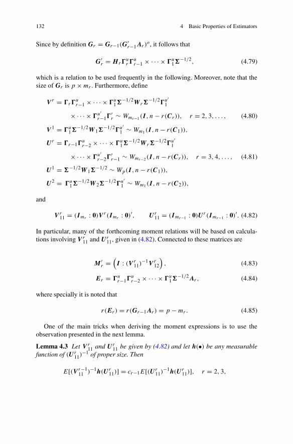
132 4 Basic Properties of Estimators
Since by definition Gr = Gr−1(G′r−1Ar )
o, it follows that
G′r = H r�
ur �
ur−1 × · · · × �u
1�−1/2, (4.79)
which is a relation to be used frequently in the following. Moreover, note that thesize of Gr is p × mr . Furthermore, define
V r = �r�ur−1 × · · · × �u
1�−1/2W r�−1/2�u′
1
× · · · × �u′r−1�
′r ∼ Wmr−1(I , n − r(Cr )), r = 2, 3, . . . , (4.80)
V 1 = �u1�−1/2W 1�
−1/2�u′1 ∼ Wm1(I , n − r(C1)),
U r = �r−1�ur−2 × · · · × �u
1�−1/2W r�−1/2�u′
1
× · · · × �u′r−2�
′r−1 ∼ Wmr−2(I , n − r(Cr )), r = 3, 4, . . . , (4.81)
U1 = �−1/2W 1�−1/2 ∼ Wp(I , n − r(C1)),
U2 = �u1�−1/2W 2�
−1/2�u′1 ∼ Wm1(I , n − r(C2)),
and
V r11 = (Imr : 0)V r (Imr : 0)′, U r
11 = (Imr−1 : 0)U r (Imr−1 : 0)′. (4.82)
In particular, many of the forthcoming moment relations will be based on calcula-tions involving V r
11 and U r11, given in (4.82). Connected to these matrices are
M ′r =
(
I : (V r11)
−1V r12
)
, (4.83)
Er = �ur−1�
ur−2 × · · · × �u
1�−1/2Ar , (4.84)
where specially it is noted that
r(Er ) = r(Gr−1Ar ) = p − mr. (4.85)
One of the main tricks when deriving the moment expressions is to use theobservation presented in the next lemma.
Lemma 4.3 Let V r11 and U r
11 be given by (4.82) and let h(•) be any measurablefunction of (U r
11)−1 of proper size. Then
E[(V r−111 )−1h(U r
11)] = cr−1E[(U r11)
−1h(U r11)], r = 2, 3,
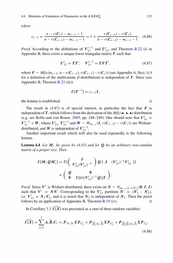
4.6 Moments of Estimators of Parameters in the EBRM3B 133
where
cr−1 = n − r(Cr ) − mr−1 − 1
n − r(Cr−1) − mr−1 − 1= 1 + r(Cr−1) − r(Cr )
n − r(Cr−1) − mr−1 − 1. (4.86)
Proof According to the definitions of V r−111 and U r
11, and Theorem B.22 (i) inAppendix B, there exists a unique lower triangular matrix T such that
U r11 = T T ′, V r−1
11 = T FT ′, (4.87)
where F ∼ MβI(mr−1, n−r(Cr−1), r(Cr−1)−r(Cr )) (see Appendix A, Sect. A.9for a definition of the multivariate β-distribution) is independent of T . Since (seeAppendix B, Theorem B.22 (iii))
E[F−1] = cr−1I ,
the lemma is established. ��The result in (4.87) is of special interest, in particular the fact that F is
independent of T , which follows from the derivation of the MβI (•, •, •) distribution(e.g. see Kollo and von Rosen, 2005, pp. 248–249). One should note that U r
11 =V r−1
11 + W , where U r11, V r−1
11 and W ∼ Wmr−1(I , r(Cr−1) − r(Cr )) are Wishart-distributed, and W is independent of V r−1
11 .Another important result which will also be used repeatedly is the following
lemma.
Lemma 4.4 Let Mr be given by (4.83) and let Q be an arbitrary non-randommatrix of a proper size. Then
E[MrQM ′r ] = E[
(
I
V r21(V
r11)
−1
)
Q(
I (V r11)
−1V r12
)]
=(
Q 00 E[tr{(V r
11)−1Q}]I
)
.
Proof Since V r is Wishart-distributed, there exists an N ∼ Nmr−1,n−r(Cr)(0, I , I )
such that V r = NN ′. Corresponding to the V r11 partition N ′ = (N ′
1 : N ′2),
i.e. V r11 = N1N
′1, and it is noted that N2 is independent of N1. Then the proof
follows by an application of Appendix B, Theorem B.19 (iv). ��In Corollary 3.3 E[X] was presented as a sum of three random variables:
E[X] =3
∑
i=1
AiBiCi = P A1,S1XP C ′
1+ P
Q′1A2,S2
XP C ′2+ P
Q′2Q′
1A3,S3XP C ′
3,
(4.88)

134 4 Basic Properties of Estimators
where
P 1 = P A1,S1,P 2 = P
Q′1A2,S2
, P 3 = PQ′
2Q′
1A3,S3, (4.89)
Q1 = I − P′1,
Q2 = I − P′2. (4.90)
The variables in (4.88) are of the same type as E[X] in the BRM but unfortunatelythe variables are not independently distributed. Now it will be shown how to derivethe dispersion matrix D[E[X]]. Note that E[E[X]] = E[X] and
D[E[X]] = D[E[X] − E[X]] = D[3
∑
i=1
P i (X − E[X])PC ′i],
This means that in order to find D[E[X]], it is sufficient to consider thedispersion
D[P r (X − E[X])PC ′r], r = 1, 2, 3,
and the covariance
C[P r (X − E[X])P C ′r,P s (X − E[X])PC ′
s], 1 ≤ r < s ≤ 3.
By summing all the necessary dispersion and covariance matrices, D[E[X]] isobtained. In the next theorem the dispersion is studied, whereas the covarianceis treated in Theorem 4.13. The final expression for D[E[X]] is presented inTheorem 4.14.
Theorem 4.12 Consider the EBRM3B presented in Definition 2.2. Let mr and cr
be defined by (4.78) and (4.86), respectively. Put
d1,2 = c1e2, d1,3 = c1c2e3, d2,3 = c2e3,
where
er = (p − mr)(n − r(Cr ) − 1)
(n − r(Cr ) − mr−1 − 1)(n − r(Cr ) − mr−1 + p − mr − 1), r = 2, 3,
(4.91)
and
fr = n − r(Cr ) − 1
n − r(Cr ) − mr − 1, r = 1, 2, 3. (4.92)

4.6 Moments of Estimators of Parameters in the EBRM3B 135
Furthermore, let
A1:i = (A1 : A2 : · · · : Ai ), A1:0 = 0 (4.93)
and define
K i = �(P Gi−1,−1 − P Gi,−1)
= A1:i (A′1:i�−1A1:i )−A′
1:i − A1:i−1(A′1:i−1�
−1A1:i−1)−A′
1:i−1,
where in particular
K1 = A1(A′1�
−1A1)−A′
1,
K2 = A1:2(A′1:2�−1A1:2)−A′
1:2 − A1(A′1�
−1A1)−A′
1,
K3 = A1:3(A′1:3�−1A1:3)−A′
1:3 − A1:2(A′1:2�−1A1:2)−A′
1:2.
Then, if er and fr are finite and positive,
D[P A1,S1(X − E[X])PC ′1] = f1P C ′
1⊗ K1, (4.94)
D[PQ′
1A2,S2(X − E[X])PC ′
2] = P C ′
2⊗ (d1,2K1 + f2K2),
D[PQ′
2Q′
1A3,S3(X − E[X])PC ′
3] = P C ′
3⊗ (d1,3K1 + d2,3K2 + f3K3),
where Qr , r = 1, 2, is defined in (4.90).
Proof It follows that the proof in principle holds for an arbitrary r , which,however, will not be highlighted. Due to independence between the “mean” andthe “residuals”
D[P r (X − E[X])P C ′r] = P C ′
r⊗ E[P r�P
′r ], r = 1, 2, 3, (4.95)
where for notational convenience P r in (4.89) is used, and therefore the crucialquantity to consider is
E[P r�P′r ].
When r = 1, relation (4.95) is immediately obtained from Theorem 4.3 (ii), sincethe expressions which have to be calculated have the same form as those used whencalculating the dispersion for the dispersion of B in the BRM , i.e.
E[P 1�P′1] = f1K1, (4.96)
where f1 is given by (4.92).

136 4 Basic Properties of Estimators
Before starting the derivation of E[P r�P′r ], r = 2, 3, some preparatory results
are stated without proofs. For r = 2 the “open sesame” relation
Q1S
−12
Q′1 = Q1
S−12 = G1(G
′1W 2G1)
−1G′1 (4.97)
will be used, where G1 and W 2 are defined in (4.73) and (4.74), respectively. Thisrelation and a similar one given below in (4.101) are two of the most importantrelations for treating the EBRM3
B theoretically, since, for example, the right-hand
side of (4.97) shows that Q1S
−12
Q′1 = Q1
S−12 is inverted Wishart-distributed, and
therefore moments are also available. Moreover, with M1 as defined in (4.83)
P 2 = Q′1P A2,G′
1W2G1,G1= P ′
G1,W−11
P A2,G′1W2G1,G1
= �1/2�′1M1H
−11 P G′
1A2,G′1W2G1
G′1
(4.98)
yields
P 2�P′2 = �1/2�′
1M1PE2,U211
P ′E2,U
211
M ′1�1�
1/2,
where E2 is defined in (4.84). Then, because V 1 is Wishart distributed, V 1 = NN ′and V 1
12 = N1N′2 for some normally distributed
N = (N ′1 : N ′
2)′ ∼ Np,n−r(C1)(0, I , I ),
implying, among other things, that N2 is independent of N1 and U 211 = V 1
11 + W ,where W ∼ Wp−r(A)(I , r(C1)− r(C2)) is independent of V 1
11. It follows, by usingLemma 4.4, that
E[P 2�P′2] = �1/2�u′
1 E[PE2,U211
P ′E2,U2
11]�u
1�1/2
+�1/2�l′1 �l
1�1/2E[tr{(V 1
11)−1P E2,U
211
P ′E2,U
211
}].
Using Lemma 4.3 and Theorem B.26 (i) in Appendix B, the expectations can becalculated:
E[PE2,U211
P ′E2,U2
11] = f2P E2,
E[tr{(V 111)
−1P E2,U211
P ′E2,U
211
}] = c1E[tr{(U211)
−1P E2,U211
P ′E2,U
211
}]
= c1E[tr{(U211)
−1P E2,U211
}] = d1,2, (4.99)

4.6 Moments of Estimators of Parameters in the EBRM3B 137
defined in the statement of the theorem. Furthermore, it can be shown that K1 andK2, also given in the statement of the theorem, satisfy
K1 = �1/2�l′1 �l
1�1/2,
K2 = �1/2�u′1 P E2�
u1�1/2,
respectively, and hence
E[P 2�P′2] = d1,2K1 + f2K2 (4.100)
has been determined.Next r = 3 is considered and the derivation follows the previous case when
r = 2. Instead of (4.97), the following equations now appear:
Q2Q1
S−13
Q′1Q
′2 = Q2
Q1S
−13 = G2(G
′2W 3G2)
−1G′2 (4.101)
and
P 3 = Q′2Q
′1P A3,G
′2W3G2,G2
= P ′G1,W
−11
P ′G2,W
−12
PA3,G′2W3G2,G2
= �1/2�′1M1�
′2M2H
−12 P G′
2A3,G′2W3G2
G′2, (4.102)
as well as
P 3�P′3 = �1/2�′
1M1�′2M2P E3,U
311
P ′E3,U
311
M ′2�2M
′1�1�
1/2.
Then, once again applying Lemma 4.4 and using V 112 = N1N
′2 for some normally
distributed N ′ = (N ′1 : N ′
2), where N2 is uncorrelated with N1, M2 and U311,
E[P 3�P′3] = �1/2�u′
1 �′2E[M2P E3,U
311
P ′E3,U
311
M ′2]�2�
u1�1/2 (4.103)
+ �1/2�l′1�l
1�1/2E[tr{(V 1
11)−1�2M2PE3,U3
11P ′
E3,U311
M ′2�
′2}].(4.104)
It is observed that E[M2P E3,U311
P ′E3,U3
11M ′
2] has the same stochastic structure as
E[P 2�P′2] and therefore the right-hand side of (4.103) equals
�1/2�u′1 �′
2E[M2P E3,U311
P ′E3,U
311
M ′2]�2�
u1�1/2
= �1/2�u′1 �u′
2 E[P E3,U311
P ′E3,U
311
]�u2�u
1�1/2
+�1/2�u′1 �l′
2�l2�
u1�1/2E[tr{(V 2
11)−1P E3,U
311
P ′E3,U
311
}].

138 4 Basic Properties of Estimators
Now Lemma 4.3 and Theorem B.26 (i) in Appendix B, yield
E[P E3,U311
P ′E3,U
311
] = f3PE3 ,
E[tr{(V 211)
−1P E3,U311
P ′E3,U
311
}] = c2E[tr{(U 311)
−1PE3,U311
P ′E3,U3
11}]
= c2E[tr{(U 311)
−1PE3,U311
}] = d2,3, (4.105)
where f3 and c2 are given in Table 4.1 and d2,3 is defined in the beginning of thetheorem. Finally, (4.104) is considered:
�1/2�l′1 �l
1�1/2E[tr{(V 1
11)−1�′
2M2PE3,U311
P ′E3,U
311
M ′2�2}]
= �1/2�l′1 �l
1�1/2c1E[tr{(U211)
−1�′2M2PE3,U3
11P ′
E3,U311
M ′2�2}]
= �1/2�l′1 �l
1�1/2
×c1E[tr{(U211)
−1�′2V
2�2�u′2 (V 2
11)−1P
E3,U311
P ′E3,U3
11(V 2
11)−1�u
2�′2V
2�2}]
= �1/2�l′1 �l
1�1/2c1E[tr{�u′2 (V 2
11)−1P
E3,U311
P ′E3,U3
11(V 2
11)−1�u2U2
11}]
= �1/2�l′1 �l
1�1/2c1E[tr{(V 211)
−1PE3,U
311
P ′E3,U3
11}],
since �′2V
2�2 = U 211 and �u
2U 211�
u′2 = V 2
11. Thus, the last expression has the sameform as the left-hand side of (4.99) and, therefore, the expectation in (4.104) equals
E[tr{(V 111)
−1�′2M2P E3,U
311
P ′E3,U
311
M ′2�2}] = d1,3.
The statement of the theorem concerning r = 3 is verified by observing that
K2 = �1/2�u′1 �l′
2 �l2�
u1�1/2, (4.106)
K3 = �1/2�u′1 �u′
2 P E3�u2�u
1�1/2.
��It is of interest to reflect on how the proof was carried out and understand thatthe main parts consist of two recursive relations, and in particular to understandwhen and why Lemmas 4.3 and 4.4 were applied. Now the covariance between theterms in
E[X] = P A1,S1XP C ′1+ P
Q′1A2,S2
XP C ′2+ P
Q′2Q′
1A3,S3XPC ′
3
is studied.

4.6 Moments of Estimators of Parameters in the EBRM3B 139
Theorem 4.13 Let r < s ≤ 3 and let the notation be the same as in Theorem 4.12and its proof. Then, for the EBRM3
B presented in Definition 2.2, if er , given inTheorem 4.12, is finite and positive,
C[P r (X − E[X])PC ′r, P s (X − E[X])PC ′
s]
={
−PC ′3⊗ d2,3K2, if r > 1,
PC ′s⊗ (d1,sK1 + Ks), if r = 1.
Proof The following proof indicates that the result holds for a general m > 3 inan EBRMm
B , if MLEs have been derived. The matrices Mr and Er given by (4.83)and (4.84) will be used. Additionally, a matrix Zr,s simplifies the presentation asfollows:
Zr,s = �ur−1�
ur−2 × · · · × �u
1�−1/2P ′Gr ,W
−1r
P ′Gr+1,W
−1r+1
× · · · × P ′Gs,W
−1s
,
2 ≤ r ≤ s, (4.107)
Z1,s = P ′G1,W
−11
P ′G2,W
−12
× · · · × P ′Gs,W
−1s
, s ≥ 1, (4.108)
Zr,s = I , r > s.
First consider the case r = 1:
E[P 1�P′s ] = E[�1/2�′
1M1�u1�1/2P ′
As,G′s−1WsGs−1,Gs
Z′1,s−1]
= �1/2�u′1 E[�u
1�1/2P ′As,G
′s−1WsGs−1,Gs
Z′2,s−1]�u
1�1/2
+E[tr{(V 111)−1�u
1�−1/2�P ′As,G
′s−1WsGs−1,Gs
Z′2,s−1}]�1/2�l′
1 �l1�1/2
= �1/2�u′1 �u
1�−1/2�E[�−1/2�u′1 × · · · × �u′
s−1P′Es,U
s−111
] (4.109)
×�us−1 × · · · × �u
1�1/2 + d1,sK1 (4.110)
= �1/2�u′1 �u
1�−1/2��−1/2�u′1 × · · · × �u′
s−1PEs�u
s−1 × · · · × �u1�1/2 + d1,sK1
= Ks + d1,sK1, (4.111)
where, among other used results, Lemma 4.4 has been applied.Now suppose r = 2 and s = 3. Note that (X − E[X])PC ′
2can be written as
(X − E[X])P C ′2
= (X − E[X])(P C ′3+ P C ′
2− P C ′
3),
where (X − E[X])P C ′3
is independent of P 2, P 3 and (X − E[X])(PC ′2− P C ′
3).
Hence,
C[P 2(X − E[X])PC ′2,P 3(X − E[X])P C ′
3] = P C ′
3⊗ E[P 2�P
′3].

140 4 Basic Properties of Estimators
Thus, from now on E[P 2�P′3] is discussed in a manner similar to the way in which
we discussed the case when r = s, and it turns out that there exists a recurrenceproperty which is somewhat easier to handle than when r = s, as in Theorem 4.12.It can be shown, using the same arguments as were used when (4.103) and (4.104)were obtained, that if one assumes that
E[
tr{(V 111)
−1�u1�−1/2P A2,G
′1W2G1,G1
�P ′A3,G
′2W3G2,G2
×G2(G′2W 2G2)
−1G′2W 2�
−1/2�u′1 }
]
= 0, (4.112)
then
E[P 2�P′3] = E[Z1,1P A2,G
′1W2G1,G1
�P ′A3,G′
2W3G2,G2Z′
1,2]= �1/2�′
1E[M1�u1�−1/2P A2,G
′1W2G1,G1
�P ′A3,G
′2W3G2,G2
Z′2,2M
′1]�1�
1/2
= �1/2�u′1 �u
1�−1/2E[PA2,G′1W2G1,G1
�P ′A3,G′
2W3G2,G2Z′
2,2]�u1�1/2. (4.113)
To verify (4.112), Lemma 4.3 together with some calculations are used. The left-hand side equals
c1E[tr{(U 211)
−1�u1�−1/2P A2,G
′1W2G1,G1
�P ′A3,G
′2W3G2,G2
×G2(G′2W 2G2)
−1G′2W 2�
−1/2�u′1 }]
= c1E[tr{�u1�−1/2P A2,G
′1W2G1,G1
�P ′A3,G′
2W3G2,G2G2(G
′2W 2G2)
−1H 2�u2}]
= c1E[tr{G′2PA2,G′
1W2G1,G1�P ′
A3,G′2W3G2,G2
G2(G′2W 2G2)
−1}] = 0,
since according to the definition of G2, given in (4.79), G′2A2 = 0, which implies
that
G′2P A2,G
′1W2G1,G1
= 0.
Continuing with (4.113), by the definition of P A2,G′1W2G1,G1
, it is obtainedthat (4.113) equals (in particular using (4.79))
�1/2�u′1 �u
1�−1/2E[(I − P ′G2,W
−12
)�P ′A3,G
′2W3G2,G2
Z′2,2]�u
1�1/2, (4.114)
which consists of a difference of two moment expressions. Concerning the firstexpression, it follows that:
�1/2�u′1 �u
1�1/2E[P ′A3,G
′2W3G2,G2
Z2,2]�u1�1/2
= �1/2�u′1 �u
1�1/2E[P ′A3,G
′2W3G2,G2
]�−1/2�u′1 �u′
2 �u2�u
1�1/2, (4.115)

4.6 Moments of Estimators of Parameters in the EBRM3B 141
since
Z′2,2�
u1�1/2 = P
G2,W−12
�−1/2�u′1 �u
1�1/2
= �−1/2�u′1 �u′
2 (V 211)
−1(V 211 : V 2
12)�2�u1�1/2,
and when in (4.115) the expectation is taken, the expression including V 212
is cancelled. Because for some normally distributed N = (N ′1 : N ′
2)′ ∼
Nm1,n−r(C2)(0, I , I ), i.e. N has independent elements and a zero mean, V 212 =
N1N′2 and in particular N2 is independent of the other random quantities in (4.115).
It appears from the following that it is not necessary to express E[P ′A3,G
′2W3G2,G2
]in (4.115).
When studying the second expression in (4.114), it can be observed that
�1/2�u′1 �u
1�−1/2E[PG2,W−1
2�P ′
A3,G′2W3G2,G2
Z2,2]�u1�1/2
= �1/2�u′1 �u′
2 �u2�u
1�1/2E[P ′A3,G′
2W3G2,G2]�−1/2�u′
1 �u′2 �u
2�u1�1/2 (4.116)
+ �1/2�u′1 �l′
2 �l2�
u1�1/2E[tr{(V 2
11)−1�u
2�u1�1/2P ′
A3,G′2W3G2,G2
�−1/2�u′1 �l′
1 }],(4.117)
since
�1/2�u′1 �u
1�−1/2P ′G2,W
−12
�P ′A3,G
′2W3G2,G2
Z2,2�u1�1/2
= �1/2�u′1 �u
1�−1/2P ′G2,W
−12
�P ′A3,G
′2W3G2,G2
PG2,W
−12
�−1/2G11�
u′1 �u
1�1/2
= �1/2�u′1 �u′
2 M2�u2�u
1�1/2P ′A3,G
′2W3G2,G2
�−1/2�u′1 �u′
2 M ′2�2�
u1�1/2,
and if one calculates the expected value of this expression, one obtains the sumof (4.116) and (4.117). However, (4.116) is identical to (4.115), since
�1/2�u′1 �u′
2 �u2�u
1�1/2G2 = �1/2�u′1 �u
1�1/2G2 = �G2.
Hence,
E[P 2�P′3] = −�1/2�u′
1 �l′2�l
2�u1�1/2
×E[tr{(V 211)
−1�u2�u
1�1/2P ′A3,G
′2W3G2,G2
�−1/2�u′1 �l′
2 }].

142 4 Basic Properties of Estimators
Finally, it is noted that, according to (4.106), K2 = �1/2�u′1 �l′
2 �l2�
u1�1/2 and using
Lemma 4.3
E[tr{(V 211)
−1�u2�u
1�1/2P ′A3,G
′2W3G2,G2
�−1/2�u′1 �u′
2 }]
= c2E[tr{(U311)
−1�u2�u
1�1/2P ′A3,G
′2W3G2,G2
�−1/2�u′1 �u′
1 }]= c2E[tr{(U3
11)−1P E3,U
311
}] = d2,3,
where E3 is given by (4.84) and the last equality follows from (4.105). All thesecalculations establish the theorem. ��
Theorems 4.12 and 4.13 imply the next result.
Theorem 4.14 Consider the EBRM3B presented in Definition 2.2 and apply the
notation used in Theorems 4.12 and 4.13. Then
D[E[X]] = D[3
∑
i=1
AiB iCi ]
= D[P A1,S1XP C ′1+ P
Q′1A2,S2
XP C ′2+ P
Q′2Q′
1A3,S3XPC ′
3]
= D[P A1,S1XP C ′1] + D[P
Q′1A2,S2
XP C ′2] + D[P
Q′2Q′
1A3,S3XPC ′
3]
+2C[PA1,S1XP C ′1,P
Q′1A2,S2
XPC ′2]
+2C[PA1,S1XP C ′1,P
Q′2Q′
1A3,S3XP C ′
3]
+2C[PQ′
1A2,S2XPC ′
2,P
Q′2Q′
1A3,S3XP C ′
3]
= f1P C ′1⊗ K1 + PC ′
2⊗ (3d1,2K1 + (f2 + 2)K2)
+PC ′3⊗ (3d1,3K1 − d2,3K2 + (f3 + 2)K3).
Now the expectation of � is considered (see Theorem 3.2 for a presentation of�). The necessary calculations will be similar, but easier than those presented above,because certain random matrices are not included in the expressions given below.
Theorem 4.15 Let K i be defined in Theorem 4.12 and let mr and cr be definedby (4.78) and (4.86), respectively. Put
gi,j = cici+1 × · · · × cj−1mj/(n − r(Cj ) − mj − 1), i < j ≤ 3,
(4.118)
gj,j = mj/(n − r(Cj ) − mj − 1),

4.6 Moments of Estimators of Parameters in the EBRM3B 143
which are supposed to be finite and positive. For the EBRM3B , let � be as in
Theorem 3.2, i.e.
n� = X(I − PC′1)X′ + Q
′1X(P C′
1− P C′
2)X′
Q1
+Q′2Q
′1X(P C′
2− PC′
3)X′
Q1Q2 + Q
′3Q
′2Q
′1XPC′
3X′
Q1Q2
Q3, (4.119)
where Qi is defined in Theorem 3.2. Then
E[n�] = (n − r(C1))� +3
∑
j=2
(r(Cj−1) − r(Cj ))
×(
j−1∑
i=1
gi,j−1K i + �Gj−1(G′j−1�Gj−1)
−1G′j−1�)
+r(C3)(
3∑
i=1
gi,3K i + �G3(G′3�G3)
−1G′3�).
Proof The proof of the theorem could be based on many of the calculationsand established relations which were used when verifying Theorems 4.12 and4.13. However, since the problem is now somewhat simpler, the proof willmainly rest on taking the expectations of squares of Zr,s , defined in (4.107)and (4.108). From the given expression of n�, it follows that the expectationsof X(I − PC ′
1)X′, Q′
1X(PC ′1− PC ′
2)X′
Q1, Q′2Q
′1X(P C ′
2− P C ′
3)X′
Q1Q2 and
Q′3Q
′2Q
′1XP C ′
3X′
Q1Q2
Q3 are needed. When obtaining the moments, Facts (i)–(iii) presented at the beginning of Sect. 4.6 will be utilized. The following momentexpressions will be used:
E[X(I − P C ′1)X′] = (n − r(C1))�,
E[X(P C ′j−1
− P C ′j)X′] = (r(Cj−1) − r(Cj ))�, j = 2, 3,
E[XP C ′3X′] = r(C3)�.
Then it follows from (4.119) that the theorem is verified if it is shown that
E[Q′1�
Q1] = g1,1K1 + �G1(G′1�G1)
−1G′1�, (4.120)
E[Q′2Q
′1�
Q1Q2] = g1,2K1 + g2,2K2 + �G2(G
′2�G2)
−1G′2�,
(4.121)
E[Q′3Q
′2Q
′1�
Q1Q2
Q3] = g1,3K1 + g2,3K2 + g3,3K3
+ �G3(G′3�G3)
−1G′3�.
(4.122)

144 4 Basic Properties of Estimators
Expression (4.120) is true, since
E[Q′1�
Q1] = E[Z1,1�Z′1,1] = �1/2�′
1E[M1M′1]�1�
1/2
= �1/2�u′1 �u
1�1/2 + �1/2�l′1 �l
1�1/2E[tr{(V 1
11)−1}]
= �G1(G′1�G1)
−1G′1� + g1,1K1,
where Mr is defined in (4.83), r = 1, and E[tr{(V 111)
−1}] follows from AppendixB, Theorem B.21 (i).
Concerning (4.121),
E[Q′2Q
′1�
Q1Q2] = E[Z1,2�Z′
1,2] = �1/2�′1E[M1Z2,2�Z′
2,2M′1]�1�
1/2
= �1/2�u′1 E[Z2,2�Z′
2,2]�u1�1/2 + �1/2�l′
1 �l1�
1/2E[tr{(V 111)
−1Z2,2�Z′2,2}]
= �1/2�u′1 �′
2E[M2M′2]�2�
u1�1/2 + c1�
1/2�l′1 �l
1�1/2E[tr{(U 2
11)−1Z2,2�Z′
2,2}]= �1/2�u′
1 �u′2 �u
2�u1�1/2 + �1/2�u′
1 �l′2 �l
2�u1�1/2E[tr{(V 2
11)−1}]
+c1�1/2�l′
1 �l1�
1/2E[tr{(V 211)
−1}]= �G2(G
′2�G2)
−1G′2� + g1,2K1 + g2,2K2.
Finally, (4.122) is presented and the ideas for proving the result are similar tothose used when calculating (4.120) and (4.121):
E[Q′3Q
′2Q
′1�
Q1Q2
Q3] = E[Z1,3�Z′1,3]
= �G3(G′3�G3)
−1G′3� + g3,3K3 + g1,3K1 + g2,3K2.
Hence, based on the above-derived formulas, it is straightforward to obtain E[X(I−P C ′
1)X′], E[Q′
1X(P C ′1
− P C ′2)X′
Q1], E[Q′2Q
′1X(P C ′
2− P C ′
3)X′
Q1Q2] and
E[Q′3Q
′2Q
′1XPC ′
3X′
Q1Q2
Q3], and then the theorem is established. ��As shown in Theorem 4.15, the estimator � is not an unbiased estimator. This is byno means unexpected, because this fact has already been observed when m = 1 inthe EBRMm
B , i.e. the BRM . It can be shown that
E[n�] = n�
+3
∑
j=2
j−1∑
i=1
(r(Cj−1) − r(Cj ))(gi,j−1 − 1)K i + r(C3)
3∑
i=1
(gi,3 − 1)K i ,

4.6 Moments of Estimators of Parameters in the EBRM3B 145
where K i , i = 1, 2, 3, are given in Theorem 4.12. Therefore, if unbiased estimatorsof K i , i = 1, 2, 3, can be found, an unbiased estimator of � is available. Copyingprevious calculations yields
E[A1(A′1�
−1A1)
−A′1] = E[A1(A
′1S
−11 A1)
−A′1] = (n − r(C1) − m1)K1,
E[Q′1A2(A
′2Q1
�−1
Q′1A2)
−A′2Q1] = E[Q′
1A2(A′2Q1
S−12
Q′1A2)
−A′2Q1]
= (n − r(C2) − m1 + p − m2)K2 + c1(p − m2)K1,
E[Q′1Q
′2A3(A
′3Q2
Q1�
−1Q
′1Q
′2A3)
−A′3Q2
Q1]= E[Q′
1Q
′2A3(A
′3Q2
Q1S
−13
Q′1Q
′2A3)
−A′3Q2
Q1]= (n − r(C3) − m2 + p − m3)K3 + c1(p − m3)K2 + c1c2(p − m3)K1.
From these expressions unbiased estimators of K i , i = 1, 2, 3, let us say K i , can beobtained which are pure functions of the MLE of �. Hence, the next theorem hasbeen established.
Theorem 4.16 With � as presented in Theorem 4.15, an unbiased estimator of �
in the EBRM3B , presented in Definition 2.2, is given by
�U = � − 1
n
3∑
j=2
j−1∑
i=1
(r(Cj−1) − r(Cj ))(gi,j−1 − 1)K i − 1
nr(C3)(
3∑
i=1
(gi,3 − 1)K i ,
where
K1 = 1
n − r(C1) − m1A1(A
′1�
−1A1)
−A′1,
K2 = 1
n − r(C2) − m1 + p − m2
Q′1A2(A
′2Q1
�−1
Q′1A2)
−A′2Q1
− c1(p − m2)
n − r(C2) − m1 + p − m2K1,
K3 = 1
n − r(C3) − m2 + p − m3
Q′1Q
′2A3(A
′3Q2
Q1�
−1Q
′1Q
′2A3)
−A′3Q2
Q1
− c1(p − m3)
n − r(C3) − m2 + p − m3
K2 − c1c2(p − m3)
n − r(C3) − m2 + p − m3
K1.
In the rest of this section D[B i ] and D[B i ], i = 1, 2, 3, will be considered. ForB3 it follows from Theorem 3.2 that
B3 = (A′3G2(G
′2W 3G2)
−1G′2A3)
−1A′3G2(G
′2W 3G2)
−1G′2XC′
3(C3C′3)
−1,
(4.123)

146 4 Basic Properties of Estimators
where G2 and W 3 are given by (4.73) and (4.74), respectively. Thus, fromCorollary 4.1 (ii), if n − k3 − m2 + q3 − 1 > 0,
D[B3] = n − k3 − 1
n − k3 − m2 + q3 − 1(C3C
′3)
−1 ⊗ (A′3G2(G
′2�G2)
−1G′2A3)
−1.
It is now shown how to obtain the dispersion matrix for B2. Because of theassumption of uniqueness, given in Theorem 4.9 (iii),
G′1A2B2C2
can be studied, since
(A′2G1G
′1A2)
−1A′2G1G
′1A2B2C2C
′2(C2C
′2)
−1 = B2.
It has already been shown that B2 is an unbiased estimator and therefore
G′1A2(B2 − B2)C2 (4.124)
is treated. The expression in (4.124) can be rewritten as
G′1A2(B2 − B2)C2 = P G′
1A2,G′1W2G1
G′1(X − E[X] − A3(B3 − B3)C3)P C ′
2
= P G′1A2,G
′1W2G1
G′1{(X − E[X])(PC ′
2− P C ′
3) + (X − E[X])PC ′
3
−P A3,G′2W3G2,G2
(X − E[X])PC ′3}
= P G′1A2,G
′1W2G1
G′1(X − E[X])(P C ′
2− P C ′
3)
+P G′1A2,G
′1W2G1
G′1(I − P A3,G
′2W3G2,G2
)(X − E[X])PC ′3. (4.125)
The idea behind the decomposition of G′1A2(B2 − B2)C2 is that the components
are partly independent: (X − E[X])PC ′3
is independent of (X − E[X])(PC ′2
−P C ′
3), P G′
1A2,G′1W2G1
G′1 and PA3,G′
2W3G2,G2, because W 2 and W 3 are independent
of XP C ′3. Hence,
C[
P G′1A2,G
′1W2G1
G′1(X − E[X])(PC ′
2− P C ′
3),
P G′1A2,G
′1W2G1
(I − P A3,G′2W3G2,G2
)(X − E[X])PC ′3
]
= 0
and therefore
D[G′1A2(B2 − B2)C2]
= D[P G′1A2,G
′1W2G1
G′1(X − E[X])(P C ′
2− P C ′
3)] (4.126)
+D[P G′1A2,G
′1W2G1
(I − P A3,G′2W3G2,G2
)(X − E[X])P C ′3]. (4.127)

4.6 Moments of Estimators of Parameters in the EBRM3B 147
The two expressions given by (4.126) and (4.127) are now treated separately. Firstly,
D[P G′1A2,G′
1W2G1G′
1(X − E[X])(PC ′2− P C ′
3)]
= (P C ′2− P C ′
3) ⊗ E[PG′
1A2,G′1W2G1
G′1�G1P
′G′
1A2,G′1W2G1
]
and the rest follows from the treatment of the BRM , e.g. see (4.23). Thus, (4.126)equals
D[P G′1A2,G
′1W2G1
G′1(X − E[X])(P C ′
2− P C ′
3)] = (P C ′
2− P C ′
3)
⊗ n − r(C2) − 1
n − r(C1) − m1 + r(G′1A2) − 1
P G′1A2,G
′1G1
G′1�G1. (4.128)
Secondly, the expression (4.127) is treated, which is somewhat more complicated tohandle. Note that
D[P G′1A2,G′
1W2G1G′
1(I − PA3,G′2W3G2,G2
)(X − E[X])P C′3] = P C′
3⊗
E[P G′1A2,G′
1W2G1G′
1(I − PA3,G′2W3G2,G2
)�(I − P ′A3,G′
2W3G2,G2)G1P
′G′
1A2,G′1W2G1
]
and
PG′1A2,G
′1W2G1
G′1 = H 1�
l′2�l
2�u1�−1/2 − H 1�
l′2 V 2
21(V211)
−1�u2�u
1�−1/2, (4.129)
where �1, �2 and H 1 are defined in (4.75) and (4.76). Then, becauseE[V 2
21(V211)
−1] = 0,
E[P G′1A2,G′
1W2G1G′
1(I − PA3,G′2W3G2,G2
)�(I − P ′A3,G′
2W3G2,G2)G1P
′G′
1A2,G′1W2G1
]
= E[H 1�l′2 �l
2�u1�−1/2(I − PA3,G′
2W3G2,G2)�(I − PA3,G′
2W3G2,G2)�−1/2�u′
1 �l′2 �l
2H′1]
+E[
H 1�l′2 V 2
21(V211)
−1�u2�u
1�−1/2(I − PA3,G′2W3G2,G2
)�(I − P ′A3,G′
2W3G2,G2)
×�−1/2�u′1 �u′
2 (V 211)
−1V 212�
l2H
′1
]
. (4.130)
The two expressions on the right-hand side of (4.130) will from now on beconsidered separately. The difference between obtaining moments for the meanparameters and obtaining moments for E[X] or � is that in the latter cases onehas not to rely on uniqueness for the mean parameters. Concerning B2, it followsfrom the proof of Theorem 4.9 (iii) that in order for B2 to be unique, C(A′
3G1) =C(A′
3G2) has to be true. Thus, utilizing (4.79),
�u1�−1/2A3 = Z�u
2�u1�−1/2A3

148 4 Basic Properties of Estimators
for some matrix Z, and
�u1�−1/2(I − P A3,G
′2W3G2,G2
)
= �u1�−1/2 − Z�l′
3�l3�
u2�u
1�−1/2 + Z�l′3 V 3
21(V311)
−1�u3�u
2�u1�−1/2.
Then, since E[V 321(V
311)
−1] = 0 and �l2�
u′2 = 0,
E[H1�l′2 �l
2�u1�−1/2(I − PA3,G
′2W3G2,G2
)�(I − P ′A3,G
′2W3G2,G2
)�−1/2�u′1 �l′
2 �l2H
′1]
= H1�l′2 �l
2H ′1 + n − r(C3) − 1
n − r(C3) − m3 − 1H 1�
l′2 �l
2Z�l′3 �l
3Z′�l′2 �l
2H′1,
where H 1�l′2�l
2H′1 and H 1�
l′2�l
2Z�l′3 �l
3Z′�l′
2 �l2H
′1 now have to be expressed in
the original matrices. A few calculations show that
�l′3�l
3 = �u2�u
1�−1/2A3(A′3G2(G
′2�G2)
−1G′2A
′3)
−A′3�
−1/2�u′1 �u′
2 , (4.131)
�l′2�l
2 = �u1�−1/2A2(A
′2G1(G
′1�G1)
−1G′1A2)
−A′2�
−1/2�u′1 , (4.132)
�u′1 �u
1 = �1/2G1(G′1�G1)
−1G′1�
1/2, (4.133)
and then (4.132) implies the relation
H 1�l′2 �l
2 = G1A2(A′2G1(G
′1�G1)
−1G′1A2)
−A′2�
−1/2�u′1
and (4.131) implies that
Z�l′3�l
3Z′ = �u
1�−1/2A3(A′3G2(G
′2�G2)
−1G′2A3)
−A′3�
−1/2�u′1 .
Moreover, using (4.133) the first expression on the right-hand side of (4.130) equals
E[H 1�l′2 �l
2�u1�−1/2(I − P A3,G′
2W3G2,G2)�(I − P ′
A3,G′2W3G2,G2
)�−1/2�u′1 �l′
2 �l2H
′1]
= n−r(C3)−1n−r(C3)−m3−1P G′
1A2,G′1G1
G′1A3(A
′3G2(G
′2�G2)
−1G′2A
′3)
−A′3G1P
′G′
1A2,G′1G1
+ PG′1A2,G′
1G1G′
1�G1. (4.134)
The second term on the right-hand side of (4.130) can after some calculations beshown to equal
E[
H 1�l′2 V 2
21(V211)
−1�u2�u
1�−1/2(I − P A3,G′2W3G2,G2
)�(I − P ′A3,G′
2W3G2,G2)�−1/2�u′
1 �u′2
×(V 211)
−1V 212�
l2H
′1
]
= H 1�l′2 �l
2H′1E[tr{(V 2
11)−1�u
2�u1�−1/2(I − PA3,G′
2W3G2,G2�(I − P ′
A3,G′2W3G2,G2
)
×�−1/2�u′1 �u′
2 }], (4.135)

4.6 Moments of Estimators of Parameters in the EBRM3B 149
and the remaining task is to obtain the expectation of the trace function in (4.135).However, the necessary calculations have by now been repeated several times andtherefore, without showing any details, it is stated that
E[tr{(V 211)
−1�u2�u
1�−1/2(I − PA3,G′2W3G2,G2
)�(I − P ′A3,G
′2W3G2,G2
)�−1/2�u′1 �u′
2 }]
= c2E[tr{(U311)−1U3
11�u′3 (V 3
11)−1(V 311)−1�u
3U311}]
= c2E[tr{(V 311)
−1}] = c2m3
n − r(C3) − m3 − 1, (4.136)
where U 311 is defined in (4.82).
Hence, by using (4.126)–(4.130), (4.134)–(4.136), D[G′1A2(B2 − B2)C2], can
be obtained and after a discussion of D[B1], a forthcoming Theorem 4.17 will bepresented where, among other things, a complete expression for D[B2] is given.
Concerning D[B1], it should be noted that the treatment of D[B1] is similar tothe treatment of D[B2], although some additional arguments are needed. If B1 isto be unique, it follows from Theorem 4.9 that A1 and C1 must be of full rank and,therefore, instead of B1, the linear combinations A1(B1 −B1)C1, with expectation0, will be studied.
As when treating (4.124), A1(B1 − B1)C1 will be decomposed, i.e.
A1(B1 − B1)C1
= P A1,W1(X − E[X])(P C′1− P C′
2)
+P A1,W1 (I − PA2,G′1W2G1,G1
)(X − E[X])(P C′2− P C′
3)
+P A1,W1 (I − PA2,G′1W2G1,G1
)(I − PA3,G′2W3G2,G2
)(X − E[X])P C′3. (4.137)
Due to independence among the terms
D[A1(B1 − B1)C1]= D[P A1,W1 (X − E[X])(P C′
1− P C′
2)]
+D[P A1,W1(I − PA2,G′1W2G1,G1
)(X − E[X])(P C′2− P C′
3)]
+D[P A1,W1(I − PA2,G′1W2G1,G1
)(I − PA3,G′2W3G2,G2
)(X − E[X])P C′3]. (4.138)
The three terms on the right-hand side of (4.138) are now treated one by one. Usingthe independence between PA1,W1 and (X − E[X])(P C ′
1− P C ′
2),
D[P A1,W1(X − E[X])(P C ′1− P C ′
2)] = (P C ′
1− P C ′
2) ⊗ E[PA1,W1�P ′
A1,W1],
and knowledge about the BRM yields
E[P A1,W1�P ′A1,W1
] = n − k1 − 1
n − k1 − p + q1 − 1A1(A
′1�
−1A1)−1A′
1. (4.139)

150 4 Basic Properties of Estimators
Concerning the second expression, it is noted that (X − E[X])(P C ′2
− P C ′3) is
independent of P A1,W1 and P A2,G′1W2G1,G1
. Hence,
D[PA1,W1 (I − PA2,G′1W2G1,G1
)(X − E[X])(PC ′2− PC ′
3)]
= (PC ′2− PC ′
3) ⊗ E[PA1,W1(I − PA2,G
′1W2G1,G1
)�(I − P ′A2,G
′1W2G1,G1
)P ′A1,W1
].(4.140)
In order to find an explicit expression of (4.140), the approach to finding theexpectation in (4.130) is copied. Rewriting PA1,W1 and PA2,G
′1W2G1,G1
in acanonical form, one obtains:
P A1,W1 = �1/2�l′1 �l
1�−1/2 − �1/2�l′
1 V 121(V
111)
−1�u1�−1/2
and
P A2,G′1W2G1,G1
= Z1H 1�l′2�l
2�u1�−1/2 − Z1H 1�
l′2V 2
21(V211)
−1�u2�u
1�−1/2,
where Z1 is defined based on the fact that the uniqueness of B1 implies C(A′2) =
C(A′2G1): hence a Z1 exists such that
A2 = Z1G′1A2.
Applying the same techniques as before gives
E[P A1,W1(I − P A2,G′1W2G1,G1
)�(I − P ′A2,G
′1W2G1,G1
)P ′A1,W1
]
= (1 + c1m2
n − r(C2) − m2 − 1)A1(A
′1�
−1A1)−1A′
1
+ n − r(C2) − 1
n − r(C2) − m2 − 1P A1,A2(A
′2G1(G
′1�G1)
−1G′1A2)
−A′2P
′A1,
.
Finally, the third term in (4.138) can be written as follows:
D[P A1,W1(I − P A2,G′1W2G1,G1
)(I − P A3,G′2W3G2,G2
)(X − E[X])P C ′3]
= P C ′3⊗ E
[
PA1,W1(I − PA2,G′1W2G1,G1
)(I − P A3,G′2W3G2,G2
)�
×(I − P ′A3,G
′2W3G2,G2
)(I − P ′A2,G
′1W2G1,G1
)P ′A1,W1
]
.

4.6 Moments of Estimators of Parameters in the EBRM3B 151
It can be shown that the expectation equals
E[�1/2�u′1 �u
1�−1/2(I − PA2,G′1W2G1,G1
)(I − PA3,G′2W3G2,G2
)�
×(I − P ′A3,G
′2W3G2,G2
)(I − P ′A2,G
′1W2G1,G1
)�−1/2�l′1 �l
1�1/2]
+E[
�1/2�l′1 V 1
21(V111)
−1�u1�−1/2(I − P A2,G
′1W2G1,G1
)(I − P A3,G′2W3G2,G2
)�
×(I − P ′A3,G
′2W3G2,G2
)(I − P ′A2,G
′1W2G1,G1
)�−1/2�u′1 (V 1
11)−1V 1
12�u1�1/2
]
,
(4.141)
where
E[
�1/2�u′1 �u
1�−1/2(I − PA2,G′1W2G1,G1
)(I − P A3,G′2W3G2,G2
)�
×(I − P ′A3,G
′2W3G2,G2
)(I − P ′A2,G
′1W2G1,G1
)�−1/2�l′1�l
1�1/2
]
= P A1,� + PA1,A2(A′2G1(G
′1�G1)
−1G′1A2)
−A′2P
′A1,
+ n−r(C3)−1n−r(C3)−m3−1P A1,(I − P A2,G
′1G1,G1
)
×A3(A′3G2(G
′2�G2)
−1G′2A3)
−A′3(I − P A2,G
′1G1,G1
)′P ′A1, (4.142)
and
E[
�1/2�l′1 V 1
21(V111)
−1�u1�−1/2(I − PA2,G
′1W2G1,G1
)(I − P A3,G′2W3G2,G2
)�
×(I − P ′A3,G
′2W3G2,G2
)(I − P ′A2,G
′1W2G1,G1
)�−1/2(�11)
′(V 111)
−1V 112�
u1�1/2
]
= A1(A′1�
−1A1)−1A′
1c1c2m3
n − r(C3) − m3 − 1. (4.143)
In the next theorem D[Bi], i = 1, 2, 3, are stated explicitly.
Theorem 4.17 Consider the EBRM3B presented in Definition 2.2. Let B i , i =
1, 2, 3, be given in Theorem 3.2 and suppose that for each Bi the uniqueness con-ditions in Theorem 4.9 are satisfied. Let Gi , mi and ci be defined by (4.73), (4.78)and (4.86), respectively. Then, if the dispersion matrices are supposed to exist,
(i) if n − k3 − m2 + q3 − 1 > 0,
D[B3] = n−k3−1n−k3−m2+q3−1 (C3C
′3)
−1 ⊗ (A′3G2(G
′2�G2)
−1G′2A3)
−1;
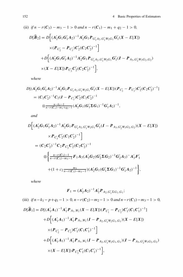
152 4 Basic Properties of Estimators
(ii) if n − r(C3) − m3 − 1 > 0 and n − r(C1) − m1 + q2 − 1 > 0,
D[B2] = D[
(A′2G1G
′1A2)
−1A′2G1PG′
1A2,G′1W2G1
G′1(X − E[X])
×(P C ′2− PC ′
3)C′
2(C2C′2)
−1]
+D[
(A′2G1G
′1A2)
−1A′2G1P G′
1A2,G′1W2G1
G′1(I − P A3,G
′2W3G2,G2
)
×(X − E[X])PC ′3C′
2(C2C′2)
−1]
,
where
D[(A′2G1G
′1A2)
−1A′2G1P G′
1A2,G′1W2G1
G′1(X − E[X])(P C′
2− PC′
3)C′
2(C2C′2)
−1]= (C2C
′2)
−1C2(I − P C′3)C′
2(C2C′2)
−1
⊗ n−k2−1n−r(C1)−m1+q2−1 (A′
2G1(G′1�G1)
−1G′1A2)
−1,
and
D[
(A′2G1G
′1A2)
−1A′2G1P G′
1A2,G′1W2G1
G′1(I − P A3,G
′2W3G2,G2
)(X − E[X])
×PC ′3C′
2(C2C′2)
−1]
= (C2C′2)
−1C2PC ′3C′
2(C2C′2)
−1
⊗{
n−r(C3)−1n−r(C3)−m3−1F 1A3(A
′3G2(G
′2�G2)
−1G′2A3)
−A′3F
′1
+(1 + c2m3
n−r(C3)−m3−1 )(A′2G1(G
′1�G1)
−1G′1A2)
−1}
,
where
F 1 = (A′2A2)
−1A′2P A2,G
′1G1,G1
;(iii) if n−k1−p+q1−1 > 0, n−r(C2)−m2−1 > 0 and n−r(C3)−m3−1 > 0,
D[B1] = D[(A′1A1)
−1A′1P A1,W1(X − E[X])(PC ′
1− P C ′
2)C′
1(C1C′1)
−1]
+D[
(A′1A1)
−1A′1PA1,W1(I − PA2,G′
1W2G1,G1)(X − E[X])
×(P C ′2− P C ′
3)C′
1(C1C′1)
−1]
+D[
(A′1A1)
−1A′1PA1,W1(I − PA2,G′
1W2G1,G1)(I − P A3,G
′2W3G2,G2
)
×(X − E[X])P C ′3C′
1(C1C′1)
−1]
,

4.6 Moments of Estimators of Parameters in the EBRM3B 153
where
D[(A′1A1)
−1A′1PA1,W1(X − E[X])(P C′
1− PC′
2)C ′
1(C1C′1)
−1]= (C1C
′1)
−1C1(I − PC′2)C′
1(C1C′1)
−1 ⊗ n−k1−1n−k1−p+q1−1 (A′
1�−1A1)
−1,
D[(A′1A1)
−1A1PA1,W1(I − P A2,G′1W2G1,G1
)(X − E[X])(P C′2− PC′
3)C ′
1(C1C′1)
−1]= (C1C
′1)
−1C1(P C′2− PC′
3)C ′
1(C1C′1)
−1
⊗{
(1 + c1m2
n−r(C2)−m2−1 )(A′1�
−1A1)−1
+ n−r(C2)−1n−r(C2)−m2−1F 2A2(A
′2G1(G
′1�G1)
−1G′1A2)
−A′2F
′2
}
with
F 2 = (A′1A1)
−1A′1PA1, (4.144)
and
D[
(A′1A1)
−1A′1P A1,W1(I − P A2,G
′1W2G1,G1
)(I − P A3,G′2W3G2,G2
)
×(X − E[X])PC ′3C′
1(C1C′1)
−1]
= (C1C′1)
−1C1P C ′3C′
1(C1C′1)
−1
⊗{
(1 + c1c2m3
n−r(C3)−m3−1 )(A′1�
−1A1)−1
+F 2A2(A′2G1(G
′1�G1)
−1G′1A2)
−A′2F
′2
+ n−r(C3)−1n−r(C3)−m3−1F 3A3(A
′3G2(G
′2�G2)
−1G′2A3)
−A′3F
′3
}
,
where
F 3 = (A′1A1)
−1A′1P A1,(I − P A2,G
′1G1,G1
). (4.145)
In Theorem 4.17 D[B i], i = 1, 2, 3, was presented. However, in order to applythe results, estimators of these quantities are needed. Now estimators based on the

154 4 Basic Properties of Estimators
MLEs are derived, and according to Theorem 4.17, these estimators are immediatelyobtained if unbiased estimators of L1 − L6, given below, are found:
L1 = (A′3G2(G
′2�G2)
−1G′2A3)
−1, L2 = (A′2G1(G
′1�G1)
−1G′1A2)
−1,
L3 = (A′1�
−1A1)−1, L4 = F 1A3(A
′3G2(G
′2�G2)
−1G′2A3)
−A′3F
′1,
L5 = F 2A2(A′2G1(G
′1�G1)
−1G′1A2)
−A′2F
′2,
L6 = F 3A3(A′3G2(G
′2�G2)
−1G′2A3)
−A′3F
′3.
An unbiased estimator of L1, let us say L1, is given by
L1 = n
n − r(C3) − m2 + r(A′3G2)
(A′3Q2
Q1�
−1Q
′1Q
′2A3)
−1, (4.146)
since Q2Q1(n
�)−1Q
′1Q
′2 = G2(G
′2W 3G2)
−1G′2, G′
2W 3G2 ∼ Wm2(G′2�G2, n−
r(C3)), and then Appendix B, Theorem B.21 (i) gives the result.For the same reasons, an unbiased estimator of L2 equals
L2 = n
n − r(C2) − m1 + r(A′2G1)
(A′2Q1
�−1
Q′1A2)
−1, (4.147)
since Q1(n�)−1
Q′1 = G1(G
′1W 2G1)
−1G′1, G′
1W 2G1 ∼ Wm1(G′1�G1, n −
r(C2)), and once again Theorem B.21 (i) in Appendix B gives the result. Moreover,since
E[(A′1(n
�)−1A1)−1] = E[(A′
1S−11 A1)
−1] = (n − r(C1) − p + r(A1))
×(A′1�
−1A1)−1,
L3 = n
n − r(C1) − p + r(A1)(A′
1�
−1A1)
−1. (4.148)
Concerning L4–L6 the situation is slightly more complicated. Details of how toobtain L4 are presented, whereas the other estimators are only listed. Inspired bythe handling of (4.127),
E[PG′1A2,G
′1W2G1
G′1A3(A
′3G2(G
′2W 3G2)
−1A′3G1P
′G′
1A2,G′1W2G1
] (4.149)
is now studied. From (4.129) it follows that the expectation in (4.149) equals
H 1�l′2�l
2�u1�−1/2A3E[(A3G2(G
′2W 3G2)
−1G′2A3)
−1]A′3�
−1/2�u′1 �l′
2 �l2H
′1
+H 1�l′2 �l
2H′1E[tr{(V 2
11)−1E3(E
′3(U
311)
−1E3)−1E′
3}],

4.6 Moments of Estimators of Parameters in the EBRM3B 155
where H 1, �1, �2 are defined in (4.75) and (4.76), and E3 is defined in (4.84). Theformula comprises two expectations which have been calculated before; i.e. they aregiven by
(n − r(C3) − m2 − r(A′3G2))H 1�
l′2�l
2�u1�−1/2A3(A3G2(G
′2�G2)
−1G′2A3)
−1
×A′3�
−1/2�u′1 �l′
2 �l2H
′1
= (n − r(C3) − m2 + r(A′3G2))P G′
1A2,G′1G1
G1(A3G2(G′2�G2)
−1G′2A3)
−1
×A′3G2P
′G′
1A2,G′1G1
and
c2(p − m3)H 1�l′2 �l
2H′1 = c2(p − m3)P G′
1A2,G′1G1
G′1�G1,
respectively. Hence, once again using
G2(G′2W 3G2)
−1G′2 = Q2
Q1(n�)−1
Q′1Q
′2, (4.150)
G1(G′1W 2G1)
−1G′1 = Q1(n�)−1
Q′1, (4.151)
it can be shown that
L4 = (n − r(C3) − m2 + r(A′3G2))
−1(A′2G1G
′1A2)
−1A′2G1PG′
1A2,G′1W2G1
×G′1A3(A
′3G2(G
′2W 3G2)
−1G′2A3)
−1A′3G1P
′G′
1A2,G′1W2G1
G′1A2(A
′2G1G
′1A2)
−1
−c2(p − m3)(n − r(C3) − m2 + r(A′3G2))
−1L2 (4.152)
is an unbiased estimator of L4. Note that in the above relation, if one uses (4.150)and (4.151), L4 is explicitly expressible as a function of �.
Similar calculations yield that an unbiased estimator of L5 is given by
L5 = (n − r(C2) − m1 + r(A′2G1))
−1(A′1A1)
−1A′1PA1,S1
×A2(A′2G1(G
′1W 2G1)
−1G′1A2)
−A′2G1P
′G′
1A2,G′1W2G1
PA1,S1A1(A′1A1)
−1
−c1(p − m2)(n − r(C2) − m1 + r(A′2G1))
−1L3, (4.153)
which is expressible as a function of � via (4.151). Concerning L6, an unbiasedestimator equals
L6 = (n − r(C3) − m2 + r(A′3G2))
−1(A′1A1)
−1A′1P A1,S1(I − P A2,G′
1W2G1,G1)
×A3(A′3G2(G
′2W 3G2)
−1G′2A3)
−A′3(I − PA2,G′
1W2G1,G1)′PA1,S1A1(A
′1A1)
−1
−c1(p − m3)(A′1A1)
−1A′1(L5 − c2L3)A1(A
′1A1)
−1, (4.154)

156 4 Basic Properties of Estimators
where (4.150) and (4.151) can be used to express the estimator through �.
Theorem 4.18 Consider the EBRM3B presented in Definition 2.2. Let D[B i],
i = 1, 2, 3, be given in Theorem 4.17 and suppose that for each Bi the uniquenessconditions in Theorem 4.9 are satisfied. Let for i=1,2,3, Gi , mi and ci be definedby (4.73), (4.78) and (4.86), respectively, and let Li , i = 1, 2, 3, 4, 5, 6, be definedby (4.146)–(4.148), (4.152)–(4.154). Then, if the estimators exist:
(i)
D[B3] = n−k3−1n−k3−m2+q3−1 (C3C
′3)
−1 ⊗ L1;
(ii)
D[B2] = D[
(A′2G1G
′1A2)
−1A′2G1P G′
1A2,G′1W2G1
G′1(X − E[X])
×(P C ′2− P C ′
3)C′
2(C2C′2)
−1]
+D[
(A′2G1G
′1A2)
−1A′2G1P G′
1A2,G′1W2G1
G′1(I − PA3,G′
2W3G2,G2)
×(X − E[X])PC ′3C′
2(C2C′2)
−1]
,
where
D[
(A′2G1G
′1A2)
−1A′2G1P G′
1A2,G′1W2G1
G′1(X − E[X])
× (P C ′2− P C ′
3)C′
2(C2C′2)
−1]
= (C2C′2)
−1C2(P C ′2− P C ′
3)C′
2(C2C′2)
−1 ⊗ n−k2−1n−r(C1)−m1+q2−1
L2,
and
D[
(A′2G1G
′1A2)
−1A′2G1P G′
1A2,G′1W2G1
G′1(I − P A3,G
′2W3G2,G2
)(X − E[X])
×PC ′3C′
2(C2C′2)
−1]
= (C2C′2)
−1C2PC ′3C′
2(C2C′2)
−1
⊗{ n−r(C3)−1n−r(C3)−m3−1
L4 + (1 + c2m3
n−r(C3)−m3−1 )L2};

4.7 EBRM3W and Uniqueness Conditions for MLEs 157
(iii)
D[B1] = D[(A′1A1)
−1A′1P A1,W1(X − E[X])(PC ′
1− P C ′
2)C′
1(C1C′1)
−1]
+D[
(A′1A1)
−1A′1PA1,W1(I − PA2,G′
1W2G1,G1)(X − E[X])
×(P C ′2− P C ′
3)C′
1(C1C′1)
−1]
+D[
(A′1A1)
−1A′1PA1,W1(I − PA2,G′
1W2G1,G1)(I − P A3,G
′2W3G2,G2
)
×(X − E[X])P C ′3C′
1(C1C′1)
−1]
,
where
D[(A′1A1)
−1A′1PA1,W1(X − E[X])(PC ′
1− PC ′
2)C′
1(C1C′1)
−1]= (C1C
′1)
−1C1(P C ′1− P C ′
2)C′
1(C1C′1)
−1 ⊗ n−k1−1n−k1−p+q1−1
L3,
D[(A′1A1)
−1A1R0(I − P A3,G′2W3G2,G2
)(X − E[X])(PC ′2− PC ′
3)C′
1(C1C′1)
−1]= (C1C
′1)
−1C1(P C ′2− P C ′
3)C′
1(C1C′1)
−1
⊗{(1 + c1m2
n−r(C2)−m2−1 )L3n−r(C2)−1
n−r(C2)−m2−1L5}
and
D[
(A′1A1)
−1A′1P A1,W1(I − PA2,G
′1W2G1,G1
)(I − P A3,G′2W3G2,G2
)
×(X − E[X])P C ′3C′
1(C1C′1)
−1]
= (C1C′1)
−1C1P C ′3C′
1(C1C′1)
−1
⊗{(1 + c1c2m3
n−r(C3)−m3−1 )L3 + L5 + n−r(C3)−1n−r(C3)−m3−1
L6}.
4.7 EBRM3W
and Uniqueness Conditions for MLEs
The EBRM3W is presented in Definition 2.3 and our study of this model in this
section and the following sections includes fewer details than were provided for theEBRM3
B in the previous section. For definitions of the matrices used in Sects. 4.7–4.9 the reader is referred to Chap. 3. The difference between the treatments of thetwo models will be highlighted, but usually only theorems containing the results are

158 4 Basic Properties of Estimators
stated without proofs. Indeed, if one has followed the treatment of the EBRM3B ,
the proofs can be considered as classroom exercises. Estimators for the parametersof the EBRM3
W were given in Theorem 3.3, and in Corollary 3.4 the estimator
E[X] was presented. As before, E[X] and � are always unique. When treatingthe EBRM3
B , it was noted that the uniqueness of estimators is independent of theestimated inner product. Thus, by assuming � = I , the next theorem can be verifiedby transposing the matrices in the EBRM3
B and applying Theorem 4.9.
Theorem 4.19 Consider the EBRM3W presented in Definition 2.3. Let B i , i =
1, 2, 3, be given in Theorem 3.3 and let KB iL, i = 1, 2, 3, be linear combinationsof Bi ; K and L are known matrices of proper sizes. Then the following statementshold:
(i) B3 is unique if and only if
r(A3) = q3, r(C3) = k3, C(C′3) ∩ C(C′
1 : C′2) = {0};
(ii) KB3L is unique if and only if
C(K ′) ⊆ C(A′3), C(L′) ⊆ C(C3(C
′1 : C′
2)o);
(iii) B2 is unique if and only if
r(A2) = q2, r(C2) = k2, C(C′1) ∩ C(C′
2) = {0},C(C′
1)⊥ ∩ C(C′
1 : C′2) ∩ C(C′
1 : C′3) = {0};
(iv) KB2L is unique if and only if
C(K ′) ⊆ C(A′2), C(L) ⊆ C(C2(C
′1 : C′
3)o);
(v) B1 is unique if and only if
r(A1) = q1, r(C1) = k1, C(C′1) ∩ C(C′
2) = {0},C(C′
2)⊥ ∩ C(C′
1 : C′2) ∩ C(C′
2 : C′3) = {0};
(vi) KB1L is unique if and only if
C(K ′) ⊆ C(A′1), C(L) ⊆ C(C1),
C(C3(I − P (C ′1)
oC′2(C2P (C ′
1)oC′
2)−C2)C
′1(C1C
′1)
−L) ⊆ C(C3(C′1 : C′
2)o),
C(C2C′1(C1C
′1)
−L) ⊆ C(C2(C′1)
o).

4.8 Asymptotic Properties of Estimators of Parameters in the EBRM3W 159
4.8 Asymptotic Properties of Estimators of Parametersin the EBRM3
W
Concerning asymptotic properties we can once again rely completely on theapproach and results for the EBRM3
B . Correspondingly to Lemma 4.2 the nextlemma can be stated, whose proof follows directly from the proof of Lemma 4.2.
Lemma 4.5 Let S1, S2 and S3 be as in Theorem 3.3. Suppose that for large n,r(C1) ≤ k1, and that both r(C1 : C2 : C3) − r(C1 : C2) and r(C1 : C2) − r(C1)
do not depend on n. Then, if n → ∞,
n−1S1P→ �, n−1
S2P→ �, n−1
S3P→ �.
The following limiting quantities will be used:
KB3L = K(A′3�A3)
−A′3�XQ2C
′3(C3Q2C
′3)
−L, (4.155)
KB2L = K(A′2�
−1A2)−A′
2�−1(X − A3B3C3)Q1C
′2(C2Q1C
′2)
−L, (4.156)
KB1L = K(A′1�
−1A1)−A′
1�−1(X − A2B2C2 − A3B3C3)C
′1(C1C
′1)
−L,
(4.157)
which all are normally distributed, and where it is supposed that K and L are sochosen that (4.155)–(4.157) do not depend on the choice of g-inverses, i.e. areunique. The matrices Q1 and Q2 are defined in (3.27), i.e. Q1 = I − P C ′
1and
Q2 = I − P C ′1:C ′
2.
Correspondingly to Theorem 4.10, where the EBRM3B was considered, the next
theorem can be verified.
Theorem 4.20 Consider the EBRM3W presented in Definition 2.3. Let for i=1,2,3,
Bi and� be the maximum likelihood estimators ofB i and� in theEBRM3W , given
in Theorem 3.3.
(i) If KB3L for the specific known matrices K and L is unique for some n, andif additionally there exists a number, v, such that C(L) ⊆ C(C3Q2v), whereC3Q2v is a matrix whose columns are identical to the first v columns inC3Q2,
then KB3L − KB3LP→ 0, n → ∞, where KB3L is given by (4.155).
(ii) If KB2L for the specific known matrices K and L is unique for some n, andif additionally there exists a number, v, such that C(L) ⊆ C(C2Q1v), whereC2Q1v is a matrix whose columns are identical to the first v columns inC2Q1,
then KB2L − KB2LP→ 0, n → ∞, where KB2L is given by (4.156).
(iii) If KB1L for the specific known matrices K and L is unique for some n, andif additionally there exists a number, v, such that C(L) ⊆ C(C1v), where C1v

160 4 Basic Properties of Estimators
is a matrix whose columns are identical to the first v columns in C1, then
KB1L − KB1LP→ 0, n → ∞, where KB1L is given by (4.157).
(iv) Let Xv , C1v , C2v and C3v denote the first v columns in X, C1, C2 and C3,respectively. Then for E|Xv] = ∑3
i=1 AiB iCiv
E|Xv] − (A1B1C1v + A2B2C2v + A3B3C3v)P→ 0, n → ∞,
where A1B1C1v follows from statement (iii) by choosing K = A1 and L =C1v , A2B2C2v follows from statement (ii) by choosing K = A2 and L =C2v , and A1B3C3v follows from statement (i) by choosing K = A3 andL = C3v .
(v) Let S3 = S1 + P ′Ao
3,−1XP 3X′P Ao
3,−1 + P ′Ao
2,−1XP 2X
′P Ao2,
−1 with P 3
and P 2 defined in (3.27). Then
� − 1
n(S3 + P ′
Ao1,
−1XP C ′1X′P Ao
1,−1)
P→ 0, n → ∞.
(vi) �P→ �, n → ∞.
4.9 Moments of Estimators of Parameters in the EBRM3W
Let, as in Theorem 3.3, S1, S2 and S3 be defined by
S1 = X(I − PC ′1:C ′
2:C ′3)X′, S2 = S1 + P ′
Ao3,S−1
1XPQ2C
′3X′P
Ao3,S−1
1,
S3 = S2 + P ′Ao
2,S−1
2XP Q1C
′2X′P
Ao2,S−1
2,
where the projections Q1 = I − PC ′1
and Q2 = I − P C ′1:C ′
2. Similar to the facts
for the estimators in the EBRM3B , stated at the beginning of Sect. 4.6, the following
facts now hold.
Facts
(i) XC ′1 is independent of XQ1C
′2 and XQ2C
′3.
(ii) XQ1C′2 is independent of XQ2C
′3.
(iii) S1 is independent of XQ2C′3, XQ1C
′2 and XC′
1.(iv) S2 is independent of XQ1C
′2 and XC′
1.(v) S3 is independent of XC′
1.
Using these statements, correspondingly to Theorem 4.11, the next theorem canbe stated concerning the unbiasedness of the mean parameter estimators in theEBRM3
W .

4.9 Moments of Estimators of Parameters in the EBRM3W 161
Theorem 4.21 Consider the EBRM3W presented in Definition 2.3. Under the
uniqueness conditions given in Theorem 4.19, KBiL is an unbiased estimator ofKB iL, i = 1, 2, 3, where B i is given in Theorem 3.3.
Corollary 4.4 The expression∑3
i=1 AiBiCi is an unbiased estimator of E[X] =
∑3i=1 AiB iCi , where Bi is given in Theorem 3.3.
Many of the following moment expressions rest on the next lemma, for examplewhen considering E[n�] and D[KB iL], i = 1, 2, 3.
Lemma 4.6 Let all the matrices be as in Theorem 3.3. Then,
(i) if n − r(C′1 : C ′
2 : C′3) − 1 > 0,
E[PA3,S1�P ′A3,S1
] = n−r(C′1:C ′
2:C ′3)−1
n−r(C′1:C ′
2:C ′3)−p+r(A3)−1A3(A
′3�
−1A3)−A′
3;
(ii) if 0 < ci < ∞, i = 1, 2, where
c1 = p−r(A2)
n−r(C′1:C ′
2)−p+r(A2)−1, c2 = n−r(C′
1:C ′2)−p+r(A3)−1
n−r(C ′1:C ′
2:C ′3)−p+r(A3)−1
,
E[P A2,S2�P ′
A2,S2] = A2(A
′2�
−1A2)−A′
2 + c1P′Ao
3,�−1A2(A′2�
−1A2)−A′
2P Ao3,�−1
+c1c2A3(A′3�
−1A3)−A′
3
= (1 + c1)A2(A′2�
−1A2)−A′
2 + c1(c2 − 1)A3(A′3�
−1A3)−A′
3;
(iii) if 0 < di < ∞, i = 1, 2, where
d1 = p−r(A1)n−r(C1)−p+r(A1)−1 , d2 = n−r(C1)−p+r(A2)−1
n−r(C′1:C ′
2)−p+r(A2)−1,
and if 0 < c2 < ∞,
E[PA1,S3�P ′
A1,S3] = (1 + d1)A1(A
′1�
−1A1)−A′
1 + d2(d2 − 1)A2(A′2�
−1A2)−A′
2
+d2d1(c2 − 1)A3(A′3�
−1A3)−A′
3.
Proof Statement (i) is almost identical to the moment expression in (4.96), which inturn followed from calculations used when proving Theorem 4.3 (ii). The differenceis that in Theorem 4.3, S ∼ Wp(�, n − r(C1)), whereas now S1 ∼ Wp(�, n −r(C′
1 : C ′2 : C′
3)).Proving statement (ii) turns out to be much more complicated than proving
statement (i). This stems from the fact thatS2 is not Wishart-distributed. Because itis easier to work with P
Ao2,S−1
2instead of PA2,S2
, the following relation will be used:
E[P A2,S2�P ′
A2,S2] = E[(I − P ′
Ao2,S−1
2)�(I − P
Ao2,S−1
2)], (4.158)

162 4 Basic Properties of Estimators
and after expansion the terms on the right-hand side of (4.158) will be consideredin detail. It appears that E[P ′
Ao2,S−1
2�] is symmetric and, therefore, in order to
determine (4.158), it suffices to consider
E[P ′Ao
2,S−12
�], (4.159)
E[P ′Ao
2,S−12
�PAo
2,S−1
2]. (4.160)
In several places the following trick of multiplying by projectors, decomposing thewhole space, will be used. It is noted that since I = P ′
Ao3,−1 +PA3, (see Appendix
B, Theorem B.11 (v)), (4.159) is identical to
E[(P ′Ao
3,−1 + PA3,)P ′Ao
2,S−12
�] = E[P ′Ao
3,�−1P′Ao
2,S−12
�]. (4.161)
Note that the expression A′3�
−1X(I −PC ′1:C ′
2:C ′3) is independent of Ao′
2 X and
Ao′3 X, and E[A′
3�−1X(I − P C ′
1:C ′2:C ′
3)] = 0, and therefore in (4.161)
E[P A3,P ′Ao
2,S−1
2�] = 0.
Moreover, put
W = S1 + XP Q2C′3X′ ∼ Wp(�, n − r(C′
1 : C′2)) (4.162)
and then the important relations
Ao′2S2A
o2 = Ao′
2 WAo2, (4.163)
Ao′3S2A
o2 = Ao′
3 WAo2 (4.164)
can be obtained, meaning that Ao′3 P ′
Ao2,S−1
2is solely a function of a Wishart variable
W and
E[P ′Ao
3,−1P′Ao
2,S−12
�] = E[P ′Ao
3,−1P
′Ao
2,W−1�] = P ′Ao
3,−1P′Ao
2,�−1�
= P ′Ao
2,−1� = � − A2(A′2�
−1A2)−A′
2, (4.165)
where Appendix B, Theorem B.20 (ix) has been applied.Next (4.160) is considered and following the above ideas it is noted that (4.160)
equals
P A3,E[P ′Ao
2,S−1
2�P
Ao2,S−1
2]P ′
A3,+ P ′
Ao3,−1E[P ′
Ao2,S−1
2�P
Ao2,S−1
2]P Ao
3,−1 .
(4.166)

4.9 Moments of Estimators of Parameters in the EBRM3W 163
This is true since P A3,E[P ′Ao
2,S−1
2�P
Ao2,S−1
2]P Ao
3,−1 = 0, which holds because
A′3�
−1X(I − PC ′1:C ′
2:C ′3) is independent of Ao′
2 X and Ao′3 X, and
E[A′3�
−1X(I − P C ′1:C ′
2:C ′3)] = 0.
Now, due to (4.163) and (4.164)
P ′Ao
3,−1E[P ′Ao
2,S−12
�PAo
2,S−12
]P Ao3,−1 = P ′
Ao3,−1E[P ′
Ao2,W−1�PAo
2,W−1 ]P Ao3,−1
= � − A2(A′2�
−1A2)−A′
2 + c1P′Ao
3,−1A2(A′2�
−1A2)−A′
2PAo3,−1 ; (4.167)
c1 in this equation and in the formulation of the lemma is determined by followingthe proof of Theorem 4.6 (i) and, in particular, by making a comparison with thederivation of (4.31), as well as by performing some calculations.
In order to complete the proof of statement (ii), the remaining task is to discuss
P A3,E[P ′Ao
2,S−12
�PAo
2,S−12
]P ′A3,. (4.168)
Now another trick is applied. Note that I = PA3,S1 +P ′Ao
3,S−11
and A3S−11 S2A
o2 = 0.
Therefore (4.168) is identical to
P A3,E[P ′Ao
3,S−11
P ′Ao
2,S−12
�PAo
2,S−12
PAo
3,S−11
]P ′A3,
= P A3,E[P ′Ao
3,S−11
P ′Ao
2,W−1�P Ao2,W
−1P Ao3,S−1
1]P ′
A3,. (4.169)
The reason for including PAo
3,S−11
in (4.168) is that S2 is not Wishart-distributed,
whereas (4.169) is a function of Wishart matrices, i.e. S1 ∼ Wp(�, n− r(C ′1 : C′
2 :C′
3)) and W ∼ Wp(�, n − r(C′1 : C′
2)), which therefore is relatively easy to treat.
Moreover, since A′3�
−1X(I − P C ′1:C ′
2:C ′3) is independent of Ao′
3 X and Ao′2 X, and
hence also independent of Ao′3 WAo
3 and Ao′2 WAo
2, (4.169) equals
P A3,�P ′A3,
E[tr{P ′Ao
2,W−1�P Ao
2,W−1Ao3(A
o′3 S1A
o3)
−1Ao′3 }]. (4.170)
For the derivation of moments of estimators in the EBRM3B , Lemma 4.3 has turned
out to be crucial and this will also be the case when exploiting the expectation ofthe trace function in (4.170). Let
V = �−1/2S1�−1/2 ∼ Wp(I , n − r(C′
1 : C′2 : C′
3)),
V 11 = (I r(Ao3)
, 0)V (I r(Ao3)
, 0)′ ∼ Wp−r(A3)(I , n − r(C′1 : C′
2 : C′3)).

164 4 Basic Properties of Estimators
Since C(Ao2) ⊆ C(Ao
3), according to the definition of W , Ao′3 P ′
Ao2,W−1�P Ao
2,W−1Ao3
is a function of V 11 and a random quantity which is independent of Ao′3 S1A
o3.
Therefore, applying Lemma 4.3 yields
E[tr{P ′Ao
2,W−1�P Ao2,W−1Ao
3(Ao′3 S1A
o3)
−1Ao′3 }]
= c2E[tr{P ′Ao
2,W−1�P Ao
2,W−1A
o3(A
o′3 WAo
3)−1Ao′
3 }]
= c2E[tr{�Ao2(A
o′2 WAo
2)−1Ao′
2 }],
where c2 is given in the statement of the lemma. Furthermore, it can be shown(Theorem B.21 (i) in Appendix B) that c1 = E[tr{�Ao
2(Ao′2 WAo
2)−1Ao′
2 }].Thus, (4.170) equals
c1c2A3(A′3�
−1A3)−A′
3, (4.171)
and (4.159) and (4.160) have been determined. By expanding (4.158) and thenusing (4.165)–(4.167) and (4.171), statement (ii) of the lemma has been verified.
Now the proof of statement (iii) is briefly described. The first observation is thatthe expectation in statement (iii) equals
E[(I − P ′Ao
1,S−1
3)�(I − P
Ao1,S−1
3)] (4.172)
and therefore
E[P ′Ao
1,S−1
3�], (4.173)
E[P ′Ao
1,S−1
3�P
Ao1,S−1
3] (4.174)
are of interest. When proving statement (ii), the decomposition C(A3) � C(A3)⊥
was used. For statement (iii), let A23 be any matrix generating C(A2) ∩ C(A3)⊥.
Thus,
C(A3) � C(A2) ∩ C(A3)⊥ � C(A2)
⊥ = C(A3) � C(A23) � C(A2)⊥,
and (4.173) is identical to
(P ′Ao
2,−1 + P A23, + P A3,)E[P ′
Ao1,S−1
3�] = E[P ′
Ao2,−1P
′Ao
1,S−1
3�],
since (P A23, + P A3,)E[P ′Ao
1,S−13
�] = 0. Furthermore, put
W 1 = W + XP Q1C′2X′ ∼ Wp(�, n − r(C1)),

4.9 Moments of Estimators of Parameters in the EBRM3W 165
and then
Ao′1S3A
o1 = Ao′
1 W 1Ao1, (4.175)
Ao′2S3A
o1 = Ao′
2 W 1Ao1. (4.176)
Hence,
E[P ′Ao
2,−1P
′Ao
1,S−13
�] = E[P ′Ao
2,−1P′Ao
1,W−11
�]= P ′
Ao2,−1P
′Ao
1,−1� = P ′
Ao1,
−1�. (4.177)
Since (4.177) is a symmetric expression, E[�PAo
1,S−13
] takes the same value as the
moment expression in (4.173).Now E[P ′
Ao1,S−1
3�P
Ao1,S−1
3] in (4.174) is derived. The first observation is that the
expectation equals
P ′Ao
2,−1E[P ′Ao
1,S−13
�PAo
1,S−13
]P Ao2,
−1 (4.178)
+PA23,E[P ′Ao
1,S−13
�PAo
1,S−1
3]P ′
A23,(4.179)
+PA3,E[P ′Ao
1,S−13
�PAo
1,S−1
3]P ′
A3,, (4.180)
which is true since P ′Ao
2,−1E[P ′
Ao1,S−1
3�P
Ao1,S−1
3]PA2, = 0 and C(A2) = C(A3)�
C(A23). The expectations (4.178)–(4.180) are derived separately and one startswith (4.178), which equals (see (4.167) for hints about calculations)
� − A1(A′1�
−1A1)−A′
1 + d1P′Ao
2,−1A1(A′1�
−1A1)−A′
1P Ao2,−1, (4.181)
where d1 is given in statement (iii) of the lemma. Since A′2S
−12
S3Ao1 = 0, (4.179)
can be written as follows:
PA23,E[P ′Ao
2,S−12
P ′Ao
1,S−13
�PAo
1,S−1
3P
Ao2,S−1
2]P ′
A23,
= PA23,E[P ′Ao
2,W−1P′Ao
1,W−11
�PAo
1,W−11
PAo2,W−1]P ′
A23,
= PA23,�P ′A23,
E[tr{P ′Ao
1,W−11
�PAo
1,W−11
Ao2(A
o′2 WAo
2)−1Ao′
2 }]. (4.182)
However, since C(Ao1) ⊆ C(Ao
2), it follows from Lemma 4.3 that (4.182) equals
d1A23(A′23�
−1A23)−A′
23E[tr{P ′Ao
1,W−11
�PAo
1,W−11
Ao2(A
o′2 W 1A
o2)
−1Ao′2 }]
= d1A23(A′23�
−1A23)−A′
23E[tr{�Ao1(A
o′1 W 1A
o1)
−1Ao′1 }]
= d2d1(A2(A′2�
−1A2)−A′
2 − A3(A′3�
−1A3)−A′
3), (4.183)

166 4 Basic Properties of Estimators
where d2 is given in statement (iii) of the lemma and
A23(A′23�
−1A23)−A′
23 = A2(A′2�
−1A2)−A′
2 − A3(A′3�
−1A3)−A′
3.
Finally, the expression for (4.180) is obtained. Since both A′3S
−11
S3Ao1 = 0 and
A′2S
−12
S3Ao1 = 0, (4.180) is identical to
P A3,E[P ′Ao
3,S−11
P ′Ao
2,S−12
P ′Ao
1,S−13
�PAo
1,S−1
3P
Ao2,S−1
2P
Ao3,S−1
1]P ′
A3,
= P A3,E[P ′Ao
3,S−11
P ′Ao
2,W−1P′Ao
1,W−11
�PAo
1,W−11
PAo2,W−1P Ao
3,S−11
]P ′A3,
and the following chain of calculations holds, i.e. (4.180) equals
P A3,�P ′A3,
E[tr{P ′Ao
2,W−1P′Ao
1,W−11
�PAo
1,W−11
PAo2,W−1Ao
3(Ao′3 S1A
o3)
−1Ao′3 }]
= c2A3(A′3�
−1A3)−A′
3E[tr{P ′Ao
1,W−11
�PAo
1,W−11
Ao2(A
o′2 WAo
2)−1Ao′
2 }]
= c2d1A3(A′3�
−1A3)−A′
3E[tr{�Ao1(A
o′1 W 1A
o1)
−1Ao′3 }]
= c2d1d2A3(A′3�
−1A3)−A′
3. (4.184)
Thus, by combining (4.172)–(4.174), (4.177), (4.183) and (4.184), the expressionfor statement (iii) of the lemma is obtained. ��In Lemma 4.6, necessary preparatory results were presented. Next they will be usedwhen deriving D[E[X]], where
E[X] − E[X] = P A1,S3(X − E[X])P C ′
1+ P A2,S2
(X − E[X])PQ1C′2
+P A3,S1(X − E[X])PQ2C′3. (4.185)
Due to independence (see Facts (i)–(iii) at the beginning of this section), thecovariances between the terms in (4.185) equal 0, i.e.
C[P A1,S3(X − E[X])PC ′
1,P A2,S2
(X − E[X])PQ1C′2] = 0,
C[P A1,S3(X − E[X])PC ′
1,P A3,S1(X − E[X])PQ2C
′3] = 0,
C[P A2,S2(X − E[X])PQ1C
′2,P A3,S1(X − E[X])PQ2C
′3] = 0.
In comparison with E[X] for the EBRM3B , where the covariances between the
terms differed from 0, the situation for the EBRM3W is somewhat simpler. Without
a proof we state the next theorem.

4.9 Moments of Estimators of Parameters in the EBRM3W 167
Theorem 4.22 Consider the EBRM3W presented in Definition 2.3, and apply the
notation used in Lemma 4.6. Then
D[E[X]] = D[P A1,S3(X − E[X])P C ′
1] + D[P A2,S2
(X − E[X])PQ1C′2]
+D[P A3,S1(X − E[X])P Q2C′3]
= P C ′1⊗ E[PA1,S3
�P ′A1,S3
] + P Q1C′2⊗ E[PA2,S2
�P ′A2,S2
]+P Q2C
′3⊗ E[P A3,S1�P ′
A3,S1],
where E[PA1,S3�P ′
A1,S3], E[PA2,S2
�P ′A2,S2
] and E[P A3,S1�P ′A3,S1
] are allgiven in Lemma 4.6.
The estimated dispersion was presented in Theorem 3.3, i.e.
n� = S3 + P ′Ao
1,S−1
3XP C ′
1X′P
Ao1,S−1
3. (4.186)
Calculating the expectation of � is relatively straightforward since the necessarymoment expressions were used in the proof of Lemma 4.6. Note that XPC ′
1is
independent ofS3, XP Q1C′2
is independent ofS2 and XP Q2C′3
is independent of S1,and that E[P ′
Ao1,S−1
3�P
Ao1,S−1
3], E[P ′
Ao2,S−1
2�P
Ao2,S−1
2] and E[P ′
Ao3,S−1
1�P
Ao3,S
−11
]are obtained in the proof of Lemma 4.6.
Theorem 4.23 Consider the EBRM3W presented in Definition 2.3, and apply the
notation used in Lemma 4.6. Then
E[n�] = E[S1] + r(Q2C′3)E[P ′
Ao3,S−1
1�P
Ao3,S
−11
]+r(Q1C
′2)E[P ′
Ao2,S−1
2�P
Ao2,S−1
2] + r(C1)E[P ′
Ao1,S−1
3�P
Ao1,S−1
3],
where
E[S1] = (n − r(C′1 : C′
2 : C′3))�,
E[P ′Ao
3,S−11
�PAo
3,S−11
] = p−r(A3)
n−r(C′1:C ′
2:C ′3)−p+r(A3)−1A3(A
′3�
−1A3)−A′
3
+Ao3(A
o′3 �Ao
3)−1Ao′
3 ,
E[P ′Ao
2,S−1
2�P
Ao2,S−1
2] = Ao
2(Ao′2 �Ao
2)−1Ao′
2 + A3(A′3�
−1A3)−A′
3
+c1P′Ao
3,−1A2(A
′2�
−1A2)−1A′
2P Ao3,
−1
+c1c2A3(A′3�
−1A3)−A′
3,

168 4 Basic Properties of Estimators
E[P ′Ao
1,S−1
3�P
Ao1,S−1
3] = Ao
1(Ao′1 �Ao
1)−1Ao′
1 + d1P′Ao
2,−1A1(A
′1�
−1A1)−
×A′1PAo
2,−1 + d1d2A23(A′23�
−1A23)−A′
23
+c2d1d2A3(A′3�
−1A3)−A′
3,
and
r(Q2C′3) = r(C′
1 : C′2 : C′
3) − r(C′1 : C′
2), r(Q1C′2) = r(C′
1 : C′2) − r(C1).
The next task is to find an unbiased estimator of �, which, according toTheorem 4.23, can be achieved if unbiased estimators of E[P ′
Ao1,S−1
3�P
Ao1,S−1
3],
E[P ′Ao
2,S−12
�PAo
2,S−1
2] and E[P ′
Ao3,S−1
1�P
Ao3,S
−11
] are established. Thus, unbiased
estimators of Ai (A′i�
−1Ai )−A′
i and Aoi (A
o′i �Ao
i )−1Ao′
i , i = 1, 2, 3, solve theproblem. One strategy for finding these unbiased estimators is to replace � by itsMLE and then, after rather lengthy calculations, to find an estimator which is solelya function of the MLE. This procedure was carried out for the EBRM3
B and theresult was presented in Theorem 4.16. However, there are many alternatives and aneasy method is to apply Appendix B, Theorems B.20 (v) and B.21 (i) to S1 and(Ao′
i S1Aoi )
−1, i.e.
Ai (A′iS
−11 Ai )
−A′i ∼ Wp(Ai (A
′i�
−1Ai )−A′
i , n − r(C′1 : C′
2 : C′3) − p + r(Ai )),
E[Ai (A′iS
−11 Ai )
−A′i ] = (n − r(C′
1 : C′2 : C′
3) − p + r(Ai ))Ai (A′i�
−1Ai )−A′
i ,
and if n − r(C′1 : C ′
2 : C′3) − p + r(Ai ) − 1 > 0
E[Aoi (A
o′i S1A
oi )
−1Ao′i ] = 1
n−r(C ′1:C ′
2:C ′3)−p+r(Ai )−1Ao
i (Ao′i �Ao
i )−1Ao′
i .
Via these relations the next lemma can be proved.
Lemma 4.7 Let S1,S2 andS3 be as in Theorem 3.3 and put
h11 = 1n−r(C′
1:C ′2:C ′
3)−p+r(A3)
p−r(A3)
n−r(C′1:C ′
2:C ′3)−p+r(A3)−1
,
h12 = n − r(C′1 : C′
2 : C′3) − p + r(A3) − 1,
h21 = n − r(C′1 : C′
2 : C′3) − p + r(A2) − 1,
h22 = 1n−r(C′
1:C ′2:C ′
3)−p+r(A3), h23 = 1
n−r(C ′1:C ′
2:C ′3)−p+r(A2)
,
h31 = n − r(C′1 : C′
2 : C′3) − p + r(A1) − 1,
h32 = 1n−r(C′
1:C ′2:C ′
3)−p+r(A1), h33 = 1
n−r(C ′1:C ′
2:C ′3)−p+r(A23)
.

4.9 Moments of Estimators of Parameters in the EBRM3W 169
Then
E[P ′Ao
3,S−11
�PAo
3,S−11
] = h11A3(A′3S
−11 A3)
−A′3 + h12A
o3(A
o′3 S1A
o3)
−1Ao′3 ,
E[P ′Ao
2,S−1
2�P
Ao2,S−1
2] = h21A
o2(A
o′2 S1A
o2)
−1Ao′2 + h22A3(A
′3S
−11 A3)
−A′3
+h23c1A2(A′2S
−11 A2)
−1A′2 − h22c1A3(A
′3S
−11 A3)
−1A′3
+h22c1c2A3(A′3S
−11 A3)
−A′3,
E[P ′Ao
1,S−1
3�P
Ao1,S−1
3] = h31A
o1(A
o′1 S1A
o1)
−1Ao′1 + h32d1A1(A
′1S
−11 A1)
−A′1
−h23c1A2(A′2S
−11 A2)
−1A′2
+h33d1d2A23(A′23S
−11 A23)
−A′23 + h22c2d1d2A3(A
′3S
−11 A3)
−A′3.
Using Lemma 4.7 the following theorem is established.
Theorem 4.24 Let � be as in Theorem 3.3. Then, for the EBRM3W presented in
Definition 2.3, an unbiased estimator of � is given by
�U = � + r(C′1:C ′
2:C ′3)
n(n−r(C′1:C ′
2:C ′3))
S1 − r(Q2C′3)
nE[P ′
Ao3,S−1
1�P
Ao3,S
−11
]
− r(Q1C′2)
nE[P ′
Ao2,S−1
2�P
Ao2,S−1
2] − r(C1)
nE[P ′
Ao1,S−1
3�P
Ao1,S−1
3],
where E[P ′Ao
3,S−11
�PAo
3,S−11
], E[P ′Ao
2,S−1
2�P
Ao2,S−1
2] and E[P ′
Ao1,S−1
3�P
Ao1,S−1
3] are
all presented in Lemma 4.7.
Now D[KB iL], i = 1, 2, 3, will be obtained for known K and L under theassumption that KBiL is unique.
Theorem 4.25 Let Bi , i = 1, 2, 3, be given in Theorem 3.3 and suppose that foreach KB iL, i = 1, 2, 3, the uniqueness conditions presented in Theorem 4.19 aresatisfied. Then, if the dispersion matrices are supposed to exist,
(i)
D[KB3L] = n−r(C ′1:C ′
2:C ′3)−1
n−r(C′1:C ′
2:C ′3)−p+r(A3)−1L′(C3Q2C
′3)
−L ⊗ K(A′3�
−1A3)−K ′;
(ii)
D[KB2L] = D[K(A′2S
−12 A2)
−A′2S
−12 (X − E[X])Q1C
′2(C2Q1C
′2)
−L]+D[K(A′
2A2)−A′
2A3(B3 − B3)C3Q1C′2(C2Q1C
′2)
−L],

170 4 Basic Properties of Estimators
where D[K(A′2S
−12 A2)
−A′2S
−12 (X − E[X])Q1C
′2(C2Q1C
′2)
−L] isobtained by applying Lemma 4.6 (ii) and D[K(A′
2A2)−A′
2A3(B3 −B3)C3Q1C
′2(C2Q1C
′2)
−L] follows from statement (i) of this theorem;(iii)
D[KB1L] = D[K(A′1S
−13 A1)
−A′1S
−13 (X − E[X])C ′
1(C1C′1)
−L]+D[K(A′
1A1)−A′
1P A2,S2XQ1C
′2(C2Q1C
′2)
−C2C′1(C1C
′1)
−L]+D[K(A′
1A1)−A′
1A3(B3 − B3)C3(I − Q1C′2(C2Q1C
′2)
−C2)C′1(C1C
′1)
−L],
where
D[K(A′1S
−13 A1)
−A′1S
−13 (X − E[X])C′
1(C1C′1)
−L]
and
D[K(A′1A1)
−A′1P A2,S2
XQ1C′2(C2Q1C
′2)
−C2C′1(C1C
′1)
−L]
are obtained by applying Lemma 4.6 (ii) and (iii), and
D[K(A′1A1)
−A′1A3(B3 − B3)C3(I − Q1C
′2(C2Q1C
′2)
−C2)C′1(C1C
′1)
−L]
follows from statement (i).
Proof Note that D[KB3L] has the same structure as D[KBL] in the BRM (seeTheorem 4.3 (ii)); i.e. the result for statement (i) follows from Theorem 4.3 (ii).
For KB2L in statement (ii) the moments are more difficult to obtain than thosefor KB3L in statement (i). It follows from the facts presented at the beginning ofSect. 4.9 that XQ1C
′2 is independent of S1 and S2, as well as XQ2C
′3. Hence
K(A′2S
−12 A2)
−A′2S
−12 (X − E[X])Q1C
′2(C2Q1C
′2)
−L
and
K(A′2A2)
−A′2A3(B3 − B3)C3Q1C
′2(C2Q1C
′2)
−L
are uncorrelated. Moreover, due to assumptions about K and the fact that C(A3) ⊆C(A2),
K(A′2S
−12 A2)
−A′2S
−12 A3 = K(A′
2A2)−A′
2A3
and therefore Lemma 4.6 (ii), together with statement (i) of this theorem, establishesstatement (ii).

4.9 Moments of Estimators of Parameters in the EBRM3W 171
Similar arguments to those used for the proof of D[KB2L] also apply toD[KB1L] in statement (iii), but these arguments are omitted here. ��
When performing inference about parameters in a model, it is important tounderstand how the estimators of these parameters are correlated. Ideally theestimators should be independently distributed, but uncorrelated estimators orestimators with low correlations are to be preferred to highly related estimators.For the BRM and its extensions, usually only statements about correlation cantake place. In the next theorem the covariances between B1, B2 and B3 arepresented. The proof is based on the facts presented at the beginning of this section,i.e. Sect. 4.9, and, since the technical treatment follows the one used when verifyingthe previous theorem, it is omitted here.
Theorem 4.26 Consider the EBRM3W presented in Definition 2.3. Let B i , i =
1, 2, 3, be given in Theorem 3.3 and suppose that for each B i , i = 1, 2, 3, theuniqueness conditions given in Theorem 4.19 are satisfied. Then, if the dispersionmatrices are supposed to exist,
(i)
C[B2,B3] = −((C2Q1C′2)
−1C2Q1C′3 ⊗ (A′
2A2)−1A′
2A3)D[B3],
where D[B3] is presented in Theorem 4.25 (i);(ii)
C[B1,B3] = −((C1C′1)
−1C1C′2 ⊗ (A′
1A1)−1A′
1A2)C[B2,B3]−((C1C
′1)
−1C1C′3 ⊗ (A′
1A1)−1A′
1A3)D[B3],
where C[B2,B3] follows from statement (i), and D[B3] follows from Theo-rem 4.25 (i);
(iii)
C[B1,B2] = −((C1C′1)
−1C1C′3 ⊗ (A′
1A1)−1A′
1A3)C[B2,B3]−((C1C
′1)
−1C1C′2 ⊗ (A′
1A1)−1A′
1A2)D[B2],
where C[B2,B3] follows from statement (i), and D[B2] follows from Theo-rem 4.25 (ii).
Corollary 4.5 Let Bi , i=1,2,3, be given in Corollary 3.5, where it is supposedthat C(C′
1) is orthogonal to C(C′2 : C′
3) and C(C′2) is orthogonal to C(C′
1 : C′3).
Then C[B1,B2] = 0, C[B1,B3] = 0 and C[B2,B3] = 0.

172 4 Basic Properties of Estimators
Problems
1 Consider the BRM presented in Definition 2.1. Use simulations to indicate thatthe MLE B is unbiased. For a given data set estimate D[B]. Moreover, show viasimulations that B is not normally distributed.
2 Consider the EBRM2W presented in Definition 2.3. Show that the MLE � is not
an unbiased estimator. Derive three different unbiased estimators of �.
3 (GMANOVA + MANOVA, continuation of Problem 2 of Chap. 3) Let
X = AB1C1 + B2C2 + E,
where all matrices are given in Problem 2 of Chap. 3. Consider the MLEs andshow their consistency, and that the estimators of the mean parameters are unbiased.Moreover, find the dispersion of the estimators of the mean parameters and E[�].4 Show the relations presented in (4.97).
5 In Example 3.1 the MLE and an “unweighted” estimator of B were presented.Moreover, an upper bound (which due to randomness is not a real upper bound)between the differences of the corresponding dispersion matrices was shown. Try tofind out via simulations how sharp this upper bound is.
6 Let X ∼ Np,n(μ,�,�). Find E[tr{XX′}] and D[tr{XX′}].7 Consider the EBRM2
W presented in Definition 2.3. Show that∑2
i=1 AiB iCi ,
where B i is the MLE of B i , i = 1, 2, is an unbiased estimator of E[X] and deriveits dispersion matrix.
8 Let X ∼ Np,n(A1B1C1 + A2B2C2 + A3B3C3,�, I ), where Bi , i = 1, 2, 3,and � are the unknown parameters,
A1 =⎛
⎝
Ip1
00
⎞
⎠ , A2 =⎛
⎝
0Ip2
0
⎞
⎠ , A3 =⎛
⎝
00
Ip3
⎞
⎠ ,
where p1 + p2 + p3 = p, and C(C′3) ⊆ C(C′
2) ⊆ C(C′1). Find the MLEs of the
parameters, as well as their asymptotic distributions.
9 In the BRM presented in Definition 2.1, suppose that FB = 0 and BG = 0hold, where F : s × q and G: k × t are known matrices. Give conditions when theMLE for B is unique.
10 In the BRM presented in Definition 2.1, suppose that FBG = 0 holds, whereF : s × q and G: k × t are known matrices. Find E[�], where � is the MLE of �.

4.9 Moments of Estimators of Parameters in the EBRM3W 173
Literature
Asymptotics for linear models (including regression models), constitutes in fact thebasis for the asymptotic results for the BRM and the EBRMm• and was presentedby Eicker (1963, 1966) (see also Drygas, 1971). Another way of contemplatingasymptotic inference is, when the inference is based on an assumption aboutnormality of errors, as in this book, to view it in the light of classical likelihoodtheory modified to handle non-identically distributed observations. Since this bookcontains explicit estimators, one can adopt some approach based on working withthe estimators directly. An alternative approach is first to study an appropriatesequence of criteria functions (loss functions, likelihood functions) and determinethat they converge for large n, i.e. many independent observations, and thereafterto utilize that the estimators obtained through minimization/maximization of thecriteria function also converge (e.g. see van der Vaart, 1998).
Essential for the interpretation of results for the BRM and the EBRMm• isthe concept of estimability. Bose (1944) formally introduced the concept andits importance is highlighted in classical Gauss-Markov theory (e.g. see Rao,1973; Wang and Chow, 1994). However, Thiele (1889) had already consideredthe estimability problem in remarkable detail (see Hald, 1981). Essential for theasymptotics applied to dispersion are the results for the sample dispersion matrixwhich is proportional to S = X(I−P C ′)X′ (following the notation of the book). Anearly work which treated the results of Lemma 4.1 is the monograph by Anderson(1958). A useful trick when obtaining asymptotically equivalent expression for theMLEs of the BRM and the EBRMm• is to apply the Cramér-Slutsky theorem (seeRao, 1973; Gut, 2013). The estimator n−1S in the projection operators convergesin probability to �, and the remaining parts of the MLEs of the mean parametersand their approximating quantities are equal in distribution. Thus, results aboutasymptotically equivalent expressions are easily obtained via the Cramér-Slutskytheorem.
Moments are used in this book to understand estimators and perform den-sity approximations (see Chap. 5) called Edgeworth-type approximations. Thesemoments are based on moments of the normal distribution, i.e. the multivariatenormal distribution and the matrix normal distribution (see Holmquist, 1988; vonRosen, 1988a), and moments from the Wishart distribution (Holmquist, 1985;Lu and Richards, 2001; Letac and Massam, 2004; Graczyk et al., 2005; Collinset al., 2014). For the most commonly used definition of the Wishart matrix (XX′,where X is matrix normally distributed) these results can be obtained from themoments of the matrix normal distribution. Moreover, moments from the inverseWishart distribution (Haff, 1982; von Rosen, 1988b, 1997; Letac and Massam,2004; Matsumoto, 2012; Collins et al., 2014), and sometimes moments for themultivariate β-distribution of type I and the multivariate β-distribution of typeII (see Kollo and von Rosen, 2005, Subsection 2.4.5) are needed when workingwith the BRM or its extensions. Many of the above-cited references on Wishartmoments and inverse Wishart moments are fairly mathematical and often based

174 4 Basic Properties of Estimators
on combinatorial theory. Wong and Hua (2000) solved some of the combinatorialproblems via differentiation. However, if one is only interested in the mean anddispersion, i.e. the first and second order moments, these moments have for a longtime been available in many texts on multivariate analysis (e.g. see Srivastava andKhatri, 1979; Kollo and von Rosen, 2005). When looking for moment relations forthe symmetric Wishart matrix, it is important to clarify which object the momentsare being derived for, i.e. whether they are being derived for the upper or lowertriangular of the Wishart matrix, W , for all elements in W or for the object W whichbelongs to the space of symmetric matrices. It is also advisable to distinguish clearlybetween real valued and complex valued vectors/matrices. Moreover, sometimesexpectations of the trace of a Wishart matrix or an inverse Wishart matrix are neededand both categories of expectations can be obtained via moments of hypergeometricfunction with Wishart arguments (e.g. see Muirhead, 1982; Watamori, 1990; Lu andRichards, 2001) or by applying some of the results derived by Letac and Massam(2004), among others.
Moments for the mean and dispersion for the BRM were first presented byGrizzle and Allen (1969) who also referred to Rao (1967) and other authors wheresimilar calculations had been performed. The other moment expressions presentedin Theorems 4.6–4.11 follow from results in von Rosen (1990) (see also Kollo andvon Rosen, 2005, Chap. 4). The moment results for the EBRM3
B mostly stem fromvon Rosen (1990) and for the corresponding results for the EBRM3
W , the reader isreferred to Filipiak von Rosen (2012).
References
Anderson, T. W. (1958). An introduction to multivariate statistical analysis. New York/London:Wiley/Chapman & Hall.
Bose, R. C. (1944). The fundamental theorem of linear estimation. In Proceedings of 31st IndianScience Congress, Part III (pp. 4–5).
Collins, B., Matsumoto, S., & Saad, N. (2014). Integration of invariant matrices and moments ofinverses of Ginibre and Wishart matrices. Journal of Multivariate Analysis, 126, 1–13.
Drygas, H. (1971). Consistency of the least squares and Gauss-Markov estimators in regressionmodels. Zeitschrift für Wahrscheinlichkeitstheorie und Verwandte Gebiete, 17, 309–326.
Eicker, F. (1963). Asymptotic normality and consistency of the least squares estimators for familiesof linear regressions. Annals of Mathematical Statistics, 34, 447–456.
Eicker, F. (1966). A multivariate central limit theorem for random linear vector forms. Annals ofMathematical Statistics, 37, 1825–1828.
Filipiak, K., & von Rosen, D. (2012). On MLEs in an extended multivariate linear growth curvemodel. Metrika, 75, 1069–1092.
Graczyk, P., Letac, G., & Massam, H. (2005). The hyperoctahedral group, symmetric grouprepresentations and the moments of the real Wishart distribution. Journal of TheoreticalProbability, 18, 1–42.
Grizzle, J. E., & Allen, D. M. (1969). Analysis of growth and dose response curves. Biometrics,25, 357–381.
Gut, A. (2013). Probability: A graduate course. Springer texts in statistics (2nd ed.). New York:Springer.

References 175
Haff, L. R. (1982). Identities for the inverse Wishart distribution with computational results inlinear and quadratic discrimination. Sankhya, Series A, 44, 245–258.
Hald, A. (1981). T.N. Thiele’s contributions to statistics. International Statistical Review, 49, 1–20.Holmquist, B. (1985). Moments and cumulants from generating functions of Hilbert space-valued
random variables and an application to the Wishart distribution. University of Lund, StatisticalResearch Report 1985:3.
Holmquist, B. (1988). Moments and cumulants of the multivariate normal distribution. StochasticAnalysis and Applications, 6, 273–278.
Kollo, T., & von Rosen, D. (1995). Minimal moments and cumulants of symmetric matrices: Anapplication to the Wishart distribution. Journal of Multivariate Analysis, 55, 149–164.
Kollo, T., & von Rosen, D. (2005). Advanced multivariate statistics with matrices. Mathematicsand its applications (Vol. 579). Dordrecht: Springer.
Letac, G., & Massam, H. (2004). All invariant moments of the Wishart distribution. ScandinavianJournal of Statistics, 31, 295–318.
Li, Y., Udén, P., & von Rosen, D. (2015). A two-step estimation method for grouped data withconnections to the extended growth curve model and partial least squares regression. Journalof Multivariate Analysis, 139, 347–359.
Lu, I.-Li., & Richards, D. St. P. (2001). MacMahon’s master theorem, representation theory, andmoments of Wishart distributions. Special issue in honor of Dominique Foata’s 65th birthday(Philadelphia, PA, 2000). Advances in Applied Mathematics, 27, 531–547.
Matsumoto, S. (2012). General moments of the inverse real Wishart distribution and orthogonalWeingarten functions. Journal of Theoretical Probability, 25, 798–822.
Muirhead, R. J. (1982). Aspects of multivariate statistical theory. New York: Wiley.Potthoff, R. F., & Roy, S. N. (1964). A generalized multivariate analysis of variance model useful
especially for growth curve problems. Biometrika, 51, 313–326.Rao, C. R. (1967). Least squares theory using an estimated dispersion matrix and its application to
measurement of signals. In Proceedings of Fifth Berkeley Symposium on Mathematical Statis-tics and Probability (Berkeley, CA, 1965/66) (Vol. I). Statistics (pp. 355–372). Berkeley:University of California Press.
Rao, C. R. (1973). Linear statistical inference and its applications. Wiley series in Probability andmathematical statistics (2nd ed.). New York: Wiley.
Srivastava, M. S., & Khatri, C. G. (1979). An introduction to multivariate statistics. New York:North-Holland.
Thiele, T. N. (1889). Forelæsninger over Almindelig Iagttagelseslære: Sandsynlighedsregning ogMindste Kvadraters Methode. København: Reitzel (in Danish).
van der Vaart, A. W. (1998). Asymptotic statistics. Cambridge series in statistical and probabilisticmathematics (Vol. 3). Cambridge: Cambridge University Press.
von Rosen, D. (1988a). Moments for matrix normal variables. Statistics, 19, 575–583.von Rosen, D. (1988b). Moments for the inverted Wishart distribution. Scandinavian Journal of
Statistics, 15, 97–109.von Rosen, D. (1990). Moments for a multivariate linear model with an application to the growth
curve model. Journal of Multivariate Analysis, 35, 243–259.von Rosen, D. (1997). On moments of the inverted Wishart distribution. Statistics, 30, 259–278.Wang, S. G., & Chow, S.-C. (1994). Advanced linear models. Theory and applications. Statistics:
Textbooks and monographs (Vol. 141). New York: Marcel Dekker.Watamori, Y. (1990). On the moments of traces of Wishart and inverted Wishart matrices. South
African Statistical Journal, 24, 153–176.Wong, C. S., & Hua, C. (2000). Evaluating matrix-variate moments through higher-order differ-
ential forms and combinatorial algorithms. Journal of Statistical Planning and Inference, 91,1–21.
Chapter 5Density Approximations
5.1 Introduction
In the previous section some of the most elementary properties, i.e. moments, of theMLEs in the BRM , EBRM3
B and EBRM3W were derived. In these models the exact
distribution of the MLEs is difficult to obtain in a useful form. Thus, one needs torely on either simulations or approximations. In general, simulations may be usefulin some particular cases, but can often become computationally demanding, forexample when used to solve distributional problems connected to high-dimensionalstatistical problems.
When finding approximations of distributions, it may be advisable to start fromthe asymptotic distribution under the assumption of a large number of independentobservations. It is a fairly natural approximation strategy that one should let theasymptotic result direct the approximation. For example, if the distribution of astatistic converges to the normal distribution, it is natural to approximate witha normal distribution. The art in this connection resides in the correction ofthe approximation for the finite number of independent observations concerned.Moreover, in any serious context it is always of interest to indicate the error ofthe approximation and the best approach here is to find a sharp upper bound of theerror.
Distributions of a statistic can be approximated in many ways, for example,by approximating the statistic itself, by approximating the characteristic functionbefore transforming it back into a density, by approximating the density functionor by directly approximating the distribution function. In this section a specialtype of density approximation will be considered which is termed Edgeworth-typeexpansion. From the derivation of this type of approximation it follows that oneapproximates the characteristic function by excluding higher terms in a Taylorseries expansion of the characteristic function. At this stage the knowledge ofmoments and cumulants is crucial. Thereafter an inverse transform is applied toobtain the density approximation. The reason for calling this type of approximation
© Springer International Publishing AG, part of Springer Nature 2018D. von Rosen, Bilinear Regression Analysis, Lecture Notes in Statistics 220,https://doi.org/10.1007/978-3-319-78784-8_5
177

178 5 Density Approximations
an Edgeworth-type expansion is that it is based on the normal distribution. However,the correct term is Gram-Charlier A series expansion. Usually the differencebetween Edgeworth and Gram-Charlier expansions lies in the organization of termsin the expansion, which then affects the approximation when series are truncated.The reason for choosing the term “Edgeworth-type expansion” is that in ourapproach we do not have to distinguish between the Gram-Charlier and Edgeworthexpansions, and at the same time, the term “Gram-Charlier expansion” is incorrectfrom a historical perspective (see Hald, 2002).
This chapter focuses mainly on the approximation of the distribution of themaximum likelihood estimators of the mean parameters. Here the results areunexpectedly beautiful. The same approach could be adopted for the estimators ofthe dispersion estimators, but in this case it is not possible to bound the errors of theapproximations and therefore no results will be presented.
5.2 Preparation
Let Y be a random matrix variable with density fY (Y o). The density fY (Y o)
should be approximated via another random variable X and its density fX(Y o), andknowledge about the cumulants for both distributions. Moreover, the approximatingdensity and the characteristic functions are going to be differentiated several timesand this will be based on the following matrix derivative.
Definition 5.1 Let Y be a function of X. The kth matrix derivative is defined by
dk Y
d Xk= d
X
dk−1 Y
d Xk−1 , k = 1, 2, . . . ,
and
d Y
d X= d vec′Y
d vecX,
d0 Y
d X0 = Y ,
where, if X ∈ Rp×q ,
d
d X= (
d
d x11, . . .
d
d xp1,
d
d x12, . . . ,
d
d xp2, . . . ,
d
d x1q
, . . . ,d
d xpq
)′.
Note that a more precise, but clumsy, notation would have been dk Y(d X)k
or dk Yd Xd X...d X
;
i.e. here in Definition 5.1, Xk does not denote the matrix power.Since the Edgeworth-type expansion is based on knowledge about multivariate
cumulants, it is necessary to define them. Let ϕX(T ) denote the characteristic

5.2 Preparation 179
function (Fourier transform),
ϕX(T ) = E[eitr(T ′X)],
where i is the imaginary unit, and then the kth cumulant ck[X] is presented in thenext definition.
Definition 5.2 Let X be a random matrix. Supposing the existence of cumulants ofX, the kth cumulant of X is given by
ck[X] = 1
ikdk ln ϕX(T )
dT k
∣
∣
∣
∣
T =0, k = 1, 2, . . . .
In particular, c1[X] = E[vecX] and c2[X] = D[X] (see Appendix B, Theo-rem B.16 (iii)). Since dY
dX= d vec′Y
dX, it follows that ck[X] = ck[vecX], which
is sometimes useful to note. There exist one-to-one relations between cumulantsof an arbitrary order and moments of an arbitrary order. Moreover, for normallydistributed variables cumulants of an order > 2 equal 0. In the following the kthderivative of a density fX(Xo) will be denoted by f k
X(Xo) and f 0X(Xo) = fX(Xo),
where the derivative is given in Definition 5.1. Now necessary notations have beenintroduced and it is time to present a result concerning multivariate Edgeworth-typeexpansions.
Theorem 5.1 Let Y and X be two random matrices of the same size with densitiesfY (Xo) and fX(Xo), respectively, both evaluated at Xo. Then
fY (Xo) = fX(Xo) − vec′(E[Y ] − E[X])f 1X(Xo)
+1
2vec′(D[Y ] − D[X] + vec(E[Y ] − E[X])vec′(E[Y ] − E[X]))vecf 2
X(Xo)
−1
6
(
vec′(c3[Y ] − c3[X]) + 3vec′(D[Y ] − D[X]) ⊗ vec′(E[Y ] − E[X])
+vec′(E[Y ] − E[X])⊗3)
vecf 3X(Xo) + . . . .
Proof Consider the trivial identity
ϕY (T ) = ϕY (T )
ϕX(T )ϕX(T ) = ϕX(T )exp{ln ϕY (T ) − ln ϕX(T )}.
Now ln ϕY (T ) − ln ϕX(T ) is, according to the above definition given in Defini-tion 5.2 of cumulants, expanded as
ln ϕY (T ) − ln ϕX(T ) =∞∑
k=1
ik
k! t′(ck[Y ] − ck[X])t⊗k−1,

180 5 Density Approximations
where t = vecT . Thus,
ϕY (t) = ϕX(t)
∞∏
k=1
exp{ 1k! it
′(ck[Y ] − ck[X])(it)⊗k−1}.
Ordering the terms in a series expansion, according to t⊗k , this relation yields
ϕY (T ) = ϕX(T )
{
1 + i(c1[Y ] − c1[X])′t
+ i2
2 vec′{c2[Y ] − c2[X] + (c1[Y ] − c1[X])(c1[Y ] − c1[X])′}t⊗2
+ i3
6
(
vec′(c3[Y ] − c3[X]) + 3vec′(c2[Y ] − c2[X]) ⊗ (c1[Y ] − c1[X])′
+(c1[Y ] − c1[X])′⊗3)
t⊗3 + · · ·}
.
Next this expression is inverted via the inverse Fourier transform; i.e. the followingrelation is utilized:
(−1)ka′vecf kX(X) = (2π)−pq
∫
Rpq
ϕX(T )a′(it)⊗ke−itr(T ′X)dT , k = 0, 1, 2, . . . ,
(5.1)
where a is an arbitrary constant (pq)k-vector, which establishes the theorem. ��The theorem shows how one density is approximated using another density viaknowledge about cumulants and derivatives of the approximating density. Theapproximation is point-wise and the approximating density does not necessarilyhave to be a real density, i.e. positive, and when integrating the approximation overall the values of X, it equals 1.
From Theorem 5.1 it follows that derivatives of densities are needed. Thus, ifthe matrix normal distribution is used, the derivatives of the corresponding normaldensity are needed; i.e. the Hermite polynomials have to be expressed, and they arepresented now in the next lemma (see Appendix A, Sect. A.13 for a definition ofHermite polynomials).
Lemma 5.1 Let X ∼ Np,n(μ,�,�). Then the generalized Hermite polynomialsof an order up to 3 equal
H0(X,μ,�,�) = 1, (5.2)
H 1(X,μ,�,�) = vec(�−1(X − μ)�−1), (5.3)
H 2(X,μ,�,�) = vec(�−1(X − μ)�−1)vec′(�−1(X − μ)�−1)
−�−1 ⊗ �−1, (5.4)

5.2 Preparation 181
H 3(X,μ,�,�) = vec(�−1(X − μ)�−1)(vec′(�−1(X − μ)�−1))⊗2
−vec(�−1(X − μ)�−1)vec′(�−1 ⊗ �−1)
−vec′(�−1(X − μ)�−1) ⊗ �−1 ⊗ �−1
−�−1 ⊗ �−1 ⊗ vec′(�−1(X − μ)�−1). (5.5)
In Theorem 5.1 no errors were presented. Next a special case is considered forwhich not only are errors presented, but also an upper bound of the error is given.Let in the next theorem | • | denote the absolute value (modulus) of a real (complex)number.
Theorem 5.2 Let Y and X be two random matrices of the same size, p × q ,with densities fY (Xo) and fX(Xo), respectively, both evaluated at Xo. Moreover,suppose that
Y = X − U , (5.6)
where X and U are independently distributed, and let u = vecU and t = vecT .Then, if m + 1 is even,
fY (Xo) = fX(Xo) +m∑
k=1
1
k!vec′E[u⊗k]vecf kX(Xo) + r
m,
where
|r m| ≤ (2π)−pq 1
(m + 1)!E[(u′)⊗m+1]∫
Rpq
t⊗m+1|ϕX(T )|dt .
Proof The proof is in principle a copy of the proof of Theorem 5.1. However, dueto the assumption Y = X − U , where X and U are independently distributed,the equations of the proof look somewhat different from those in the proof of theprevious theorem. Now let us begin to work with the trivial identity
ϕY (T ) = ϕY (T )
ϕX(T )ϕX(T ) = ϕ−U (T )ϕX(T )
= ϕX(T )(1 +m∑
k=1
(−i)k
k! t ′mk[u]t⊗(k−1) + rm(T )), (5.7)
rm(T ) = 1
(m + 1)! t′ϕm+1
−U (� � T )t⊗m, (5.8)
where ϕm+1−U (� � T ) is the m + 1 derivative of ϕ−U (� � T ) evaluated at � � T ,
� is the Hadamard product (element-wise product, see Appendix A, Sect. A.6) and� is a p × q matrix whose elements have values between 0 and 1.

182 5 Density Approximations
Next the inverse Fourier transform given in (5.1) is applied to (5.7) and (5.8).Thus, the density presented in the theorem is found and a remaining task is to findthe upper bound of
r m = (2π)−pq 1
(m + 1)!∫
Rpq
vec′ϕm+1−U (� � T )t⊗m+1exp(−itr{T ′Xo})ϕX(T )dt .
Then
|r m| ≤ (2π)−pq 1
(m + 1)!∫
Rpq
|vec′ϕm+1−U (� � T )t⊗m+1||ϕX(T )|dt
≤ (2π)−pq 1
(m + 1)!∫
Rpq
E[(u′)⊗m+1]t⊗m+1|ϕX(T )|dt,
which is identical to the statement of the theorem. ��It is interesting to note that if E[(u′)⊗m+1] and
∫
Rpq t⊗m+1|ϕX(T )|dt can becalculated, an upper bound of the error has been found. However, this does notmean that the proposed boundary is sharp. In special cases one can probably findbetter bounds.
An important approximating distribution is the normal distribution with a meanequal to 0. If X ∼ Np,n(0,�,�), then
ϕX(T ) = exp(− 12 tr{�T �T ′}),
which is real-valued. Moreover, this expression, as a function in T , is proportionalto the normal density and therefore the next corollary can be stated. The normaldistribution is, however, not the only possible choice of density.
Corollary 5.1 Let Y and X be two random matrices of the same size, p × q , withdensities fY (Xo) and the matrix normal density (see Appendix A, Sect. A.10)
fX(Xo) = (2π)−pq/2|�|−p/2|�|−q/2exp(− 12 tr{�−1Xo�
−1X′o}),
respectively, both evaluated at Xo; it is supposed that both � and � are p.d., andE[X] = E[Y ] = 0. Suppose that
Y = X − U , (5.9)
where X and U are independently distributed and let u = vecU . Then
fY (Xo) = fX(Xo) +3
∑
k=1
1
k! (−1)kE[(u′)⊗k]vecH k(Xo, 0,�,�)fX(Xo) + r 3 ,

5.2 Preparation 183
where H k(Xo, 0,�,�) follows from Lemma 5.1 and
|r 3 | ≤ (2π)−pq 1
4! |�|−q/2|�|−p/2E[(u′)⊗4]E[z⊗4]
with z ∼ Npq(0,�−1 ⊗ �−1).
It follows from the corollary that the precision of the density approximationmainly depends on E[(vecU)⊗4], which in our application can be made small whenthe number of independent observations becomes large. Indeed, U can be thoughtof as an error term when approximating Y using X. However, at the same time theeigenvalues of � and �, and E[z⊗4] play a role. The expression E[z⊗4] is given inAppendix B, Theorem B.19 (v). Thus, if it is possible to choose a structure for � and�, this can be utilized when planning experiments so that, before the experiment iscarried out, there is some guarantee that an approximation of the density will work.
Moreover, when calculating the error term of the approximation, the mean canvery well differ from 0 since under normality |ϕX(T )| is not affected by themean. Thus, Corollary 5.1 can immediately be extended by replacing fX(Xo) andH k(Xo, 0,�,�) by
(2π)−pq/2|�|−p/2|�|−q/2exp(− 12 tr{�−1(Xo − μ)�−1(Xo − μ)′})
andH k(Xo,μ,�,�),
respectively. Under these assumptions the error is still the same as in Corollary 5.1.In Corollary 5.1 it was assumed that X followed a matrix normal distribution with
mean 0. Next it is assumed that for vectors y, x and u, the relation y = x −u holds,where u is independent of the normally distributed x and, in addition, symmetricallydistributed with a mean equal to 0. Then
E[u⊗2] = vec(D[y] − D[x]).
Furthermore, noting that
H 2(xo,μ,�, 1) = �−1(xo − μ)(xo − μ)′�−1 − �−1,
the next corollary can be established.
Corollary 5.2 Let y and x be two random vectors of size p with densities fy(xo)
and
fx(xo) = (2π)−p/2|�|−1/2exp(− 12 tr{�−1(xo − μ)(xo − μ)′}),

184 5 Density Approximations
respectively, both evaluated at xo; it is supposed that � is p.d. Moreover, supposethat
y = x − u, (5.10)
where u is independent of x and symmetrically distributed with mean 0. Then
fy(xo) = fx(xo)
+ 12 tr{(D[y] − �)(�−1(xo − μ)(xo − μ)′�−1 − �−1)}fx(xo) + r
3
= (1 − 12 tr{D[y]�−1I })fx(xo)
+ 12 tr{(D[y]�−1 − I )(xo − μ)(xo − μ)′�−1}fx(xo) + r
3 ,
where
|r 3 | ≤ (2π)−p 1
4! |�|−1/2E[(u′)⊗4]E[z⊗4]
with z ∼ Np(0,�−1).
Later Corollary 5.2 will be applied when D[y] is proportional to � andthen the expressions of the corollary can be simplified further. The differenceD[y] − � is positive definite. Moreover, note the following interesting fact. Whenintegrating the approximation over xo, i.e. omitting the error term in the expansion,the integral equals 1, meaning that if the approximating density is positive, theapproximating density is also a proper density, which is very uncommon whenapplying Edgeworth-type approximations. A second interesting fact appears when,instead of independence in (5.10), only uncorrelatedness holds.
Corollary 5.3 Let y and x be two random vectors of size p with densities fy(xo)
and
fx(xo) = (2π)−p/2|�|−1/2exp(− 12 tr{�−1(xo − μ)(xo − μ)′}),
respectively, both evaluated at xo; it is supposed that � is p.d. Moreover, supposethat
y = x − u, (5.11)
where C[u, x] = 0 and u is symmetrically distributed with mean 0. Then anEdgeworth-type approximation of fy(xo), which also is a density, is given by
fx(xo) + 12 tr{(D[y] − �)(�−1(xo − μ)(xo − μ)′�−1 − �−1)}fx(xo),
provided that the approximating function is ≥ 0 for all xo.

5.3 Density Approximation for the Mean Parameter in the BRM 185
5.3 Density Approximation for the Mean Parameterin the BRM
For the BRM , presented in Definition 2.1, the density of B − B is now approxi-mated. It is assumed that B is unique, i.e. the matrices A and C are of full rank, andtherefore (see Corollary 3.1)
B − B = (A′S−1A)−1A′S−1(X − ABC)C′(CC′)−1 (5.12)
is discussed, where S ∼ Wp(�, n − k). Since (see Appendix B, Theorem B.18 (ii))
1
n − kS
P→ �, n → ∞,
a natural approximating quantity is
B − B = (A′�−1A)−1A′�−1(X − ABC)C′(CC′)−1. (5.13)
Moreover, B is normally distributed and
E[B − B] = E[B − B] = 0,
D[B] − D[B] = p − q
n − k − p + q − 1(CC′)−1 ⊗ (A′�−1A)−1, (5.14)
where (5.14) is obtained from D[B], presented in Corollary 4.1 (ii), and D[B]is established with the help of Appendix B, Theorem B.19 (iii). In many naturalapplications (CC ′)−1 will become small, or at least its elements are bounded whenn → ∞, and therefore the first two moments (cumulants) of B and B are close
to each other. We also know that B − BP→ 0 as n → ∞ (see the proof of
Theorem 4.1). Hence, many properties of B support the idea of approximating thedensity of B − B with the density of B − B. The consequences of this approachare studied now and our starting point is the next important observation:
B − B = B − B − U ,
where
U = (A′S−1A)−1A′S−1(P A, − I )(X − ABC)C′(CC′)−1.
Now (A′�−1A)−1A′�−1XC′(CC′)−1 and (PA, − I )XC′(CC ′)−1 are indepen-dent (see Appendix B, Theorem B.19 (x)) and XC′(CC′)−1 is independent of S
(see Appendix B, Theorem B.19 (viii)). Therefore, B and U are independently

186 5 Density Approximations
distributed. Hence, Theorem 5.2 can be applied and the following quantities areneeded if m = 3 is chosen in Theorem 5.2:
B − B ∼ Nq,k(0, (A′�−1A)−1, (CC′)−1),
E[U ] = 0, E[u⊗3] = 0, (u = vecU ),
E[u⊗2] = vec(D[B] − D[B]) = p − q
n − k − p + q − 1vec((CC′)−1 ⊗ (A′�−1A)−1).
The last expression above is a vectorized version of (5.14). Moreover, in order toobtain the error bound of the approximation E[u⊗4] has to be considered. Althoughit is not difficult to derive E[u⊗4] explicitly, it makes sense only to consider theorder of the error without presenting any details involving A and C. The importantobservation is that
U |S ∼ Nq,k(0, (A′S−1A)−1A′S−1�S−1A(A′S−1A)−1 − (A′�−1A)−1, (CC′)−1).
(5.15)
Now, using T and V , given in (4.19) and (4.20), respectively,
(A′S−1A)−1A′S−1�S−1A(A′S−1A)−1 − (A′�−1A)−1 = (T ′)−1V 12V−122 V −1
22 V 21T−1.
However,
Z = V 12V−1/222
is independent of V 22 (see Appendix B, Theorem B.20 (iv)), and instead of (5.15)
U |Z,V 22 ∼ Nq,k(0, (T ′)−1ZV −122 Z′T −1, (CC ′)−1)
can be studied. It follows that E[u⊗4|Z,V 22] is a linear function in ZV −122 Z′ ⊗
ZV −122 Z′, and since (see Appendix B, Theorem B.19 (vii) and Theorem B.21 (iii))
in the sense of the Loewner order (see Appendix A, Sect. A.3)
E[(ZV −122 Z′)⊗2] ≤ c
n2 I
for some specific constant c, depending on A and C, the following theorem has beenestablished.
Theorem 5.3 For the BRM presented in Definition 2.1, suppose that r(A) = q
and r(C) = k, and that
B = (A′S−1A)−1A′S−1XC′(CC′)−1.

5.3 Density Approximation for the Mean Parameter in the BRM 187
Let
B = (A′�−1A)−1A′�−1XC′(CC′)−1 ∼ Nq,k(B, (A′�−1A)−1, (CC′)−1).
Then an Edgeworth-type expansion of the density of B equals
fB(Bo) = fBE (Bo) + r
3 ,
where
fBE(Bo) = {1 − 1
2 skq + 12str{A′�−1A(Bo − B)CC ′(Bo − B)′}}fB(Bo),
s= p − q
n − k − p + q − 1, n − k − p + q − 1 > 0,
and
|r 3 | ≤ c
n2 ,
for some fixed constant c which is a function of A and C.
In general the sum of the first terms in an Edgeworth-type expansion is not a density.However, as was also observed after Corollary 5.2, the density approximation for Bgiven in Theorem 5.3 works unusually well.
Theorem 5.4 The function fBE (Bo) given in Theorem 5.3 is a density if0 < 1 − 1
2 skq .
Proof If 0 < 1 − 12skq , then fBE
(Bo) ≥ 0. Hence, it has to be shown that theintegral of fBE
(Bo) over the whole space equals 1, i.e.
∫
Rq×k
fBE(Bo)dBo = 1 − 1
2 skq + 12 sE[tr{A′�−1A(B − B)CC′(B − B)′}] = 1,
where the expectation is taken with respect to B∼Nqk(B, (A′�−1A)−1, (CC′)−1)
and equals kq . ��The density function
fY (Y o) = c|�|−n/2|�|−p/2g(tr{�−1(Y o − μ)�−1(Y o − μ)′}),
where c is a standardization constant, is of the form g(u) = u exp(−u/2), Y : p ×n,μ: p × n, � > 0: p × p, � > 0: n × n, and is the density function of a randomvariable Y with a matrix Kotz-type distribution (see Nadarajah, 2003 and AppendixA, Sect. A.10 for a definition of the Kotz-type distribution).

188 5 Density Approximations
Theorem 5.5 The distribution of BE with density fBE(Bo), given in Theorem 5.3
is a mixture of a normal distribution and a matrix Kotz-type distribution withweights 1 − 1
2 skq and 12 skq , respectively, assuming that 1 − 1
2skq > 0.
A consequence of this theorem is that the distribution of BE may be multimodal,which is an undesirable feature in that it makes it more difficult to interpret extremeobservations. However, it can be shown that if
s <2
2 + pq, (5.16)
the distribution is unimodal. This means that if p is large in relation to n, i.e. thedimension in relation to the number of independent observations is large, one mayrun into problems when interpreting estimators via the approximation. Broadlyspeaking, if the approximating distribution deviates to a large extent from thenormal distribution, then the conclusions should be carefully evaluated. However,if condition (5.16) holds, we can be reasonable confident in the validity of ourconclusions.
When showing the independence between BN and U , the bilinear structure of themodel was indeed used. The matrix U is a function of S and XC′(CC′)−1, whereasBN is a function of XC′(CC′)−1. The spaces which are involved are Rn ⊗Rp, andits decomposition, i.e. (C(C′)� C(C′)⊥)⊗ (C(A)� C(A)⊥), and the projectionson these spaces: PC ′ , I − P C ′ , P A, and I − P A, . When projecting X on thesespaces, four independent quantities are obtained: P A,XP C ′ , P A,X(I − P C ′),(I − P A,)XPC ′ and (I − P A,)X(I − P C ′). Since ABNC = P A,XP C ′ andU is a function of (I − PA,)X and X(I − P C ′), the variables BN and U areindependently distributed. Hence, vector space decomposition is also essential forthe Edgeworth-type expansion of the mean estimator in the BRM , and one shouldapply knowledge concerning the tensor space Rn ⊗ Rp in a manner similar to thatused when estimating parameters. Moreover, an interesting technical observation isthat projecting X on C(A)⊥ with an estimated inner product, i.e. (I − P A,S)X, isthe same as first projecting X on C(A)⊥ and then performing a second projectionon CS(A)⊥.
If one’s intention is to perform the inference marginally on the elements of B,then the marginal distribution will also be a mixture of a Kotz-type distribution anda normal distribution, but the influence of the Kotz part will be less in this casecompared to the case where simultaneous inference on the elements of B is takingplace. Without a proof, Theorem 5.3 is now generalized as follows.
Theorem 5.6 For the BRM , suppose that C(K ′) ⊆ C(A′) and C(L) ⊆ C(C), and
KBL = K(A′S−1A)−A′S−1XC′(CC′)−L.
Let
KBL = K(A′�−1A)−A′�−1XC′(CC′)−L
∼ N•,•(KBL,K(A′�−1A)−K ′,L(CC′)−L′).

5.3 Density Approximation for the Mean Parameter in the BRM 189
Then an Edgeworth-type expansion of the density of KBL equals
fKBL(Bo) = fKBEL(Bo) + r 3 ,
where
fKBEL(Bo) = {
1 − 12 s1r(K)r(L) + 1
2 s1tr{K ′(K(A′�−1A)−K ′)−K
× (Bo − B)L(L′(CC′)−L)−L′(Bo − B)′}}fKBL(Bo),
s1 = p − r(A)
n − r(C) − p + r(A) − 1, n − r(C) − p + r(A) − 1 > 0,
and
|r 3 | ≤ c
n2,
for some fixed constant c which is a function of A and C.
Example 5.1 In Example 3.1 different estimates of B in the BRM were presented,for example the maximum likelihood estimate (Model Ia)
B1o = (A′S−1o A)−1A′S−1
o XoC′(CC′)−1 =
(
17.4 15.80.48 0.83
)
(5.17)
and an unweighted estimate (Model Ib),
B2o = (A′A)−1A′XoC′(CC ′)−1 =
(
17.4 16.30.48 0.78
)
. (5.18)
These estimates are very close to each other and one wish to ascertain which ofthe corresponding estimators is to be preferred. A natural means of determiningthis is to compare their distributions. The unweighted estimator has a matrixnormal distribution and now Theorem 5.6 provides a density approximation which,according to the theory, is fairly accurate, i.e. Op(n−2) (see Appendix A, Sect. A.12for a definition of Op(•)).
In Fig. 5.1 the approximate distribution of B1 and the distribution of B2 arecompared. Since there are four elements in B i , i = 1, 2, the distribution is presentedvia the following pairs: (bi11,bi21), the estimated intercept and slope for girls;(bi11,bi12), the estimated intercepts for girls and boys; (bi12,bi22), the estimatedintercept and slope for boys; and (bi21,bi22), the estimated slopes for boys andgirls.
The overall conclusion when inspecting Fig. 5.1 is that there is almost no differ-ence between the distributions of the estimators B1 and B2. Note that the differentshapes in (a)–(d) are due to scaling and are not of any particular interest. Thus, fromnow on one can completely rely on B2, which, due to its well-known distribution, is

190 5 Density Approximations
(a) (b) (c) (d)
Fig. 5.1 Illustration of the distributions in Example 5.2. The first row shows for the MLE, B1 =(A′S−1A)−1A′S−1XC ′(CC ′)−1, given in (5.17), the bivariate densities for the following pairs:(b11,b21), given under (a), (b11,b12), given under (b), (b12,b22), given under (c), and (b21,b22),given under (d). The second row shows the corresponding densities for the unweighted estimatorB2 = (A′A)−1A′XC′(CC ′)−1, given in (5.18)
easier to handle than B1, for example when constructing tests concerning B. Hence,an estimator is chosen which is not the maximum likelihood estimator and thus isnot asymptotically the best estimator. Moreover, redirecting the discussion one canconclude that the density approximation presented in Theorem 5.3 seems to workwell. ��Finally, an example is presented where there are some differences between the MLEand an unweighted estimator of the mean parameters.
Example 5.2 Artificial data have been generated according to
X = ABC + E, E ∼ Np,n(0,�, I ),
where
A =
⎛
⎜
⎜
⎜
⎜
⎜
⎝
1 81 121 161 201 24
⎞
⎟
⎟
⎟
⎟
⎟
⎠
, B =(
1 32 3
)
, C =(
1′14 ⊗
(
1
0
)
: 1′14 ⊗
(
0
1
))
,

5.3 Density Approximation for the Mean Parameter in the BRM 191
� =
⎛
⎜
⎜
⎜
⎜
⎜
⎝
2 1.6 0.9 1.5 0.91.6 4 1.9 3.0 1.90.9 1.9 2 1.9 0.91.5 3.0 1.9 4 1.50.9 1.9 0.9 1.5 2
⎞
⎟
⎟
⎟
⎟
⎟
⎠
.
The correlations among the variables are medium-sized, i.e. they vary between 0.45and 0.75. If one generates data with correlations around 0.90, the estimators, due tocollinearity, start to perform poorly. With the above choice of matrices, the followingdata were generated:
X =
⎛
⎜
⎜
⎜
⎜
⎜
⎝
15.7 17.6 18.3 19.5 19.2 16.9 18.1 19.0 16.0 16.6 15.3 16.8 17.9 16.8,
26.9 29.7 28.4 24.4 23.9 25.3 26.2 27.8 26.5 27.4 29.4 25.0 27.3 26.819.3 26.9 24.9 27.4 24.7 25.7 23.6 24.3 23.6 26.2 22.1 24.5 27.3 26.0,
42.1 41.8 39.2 33.4 37.4 39.4 39.9 40.4 36.4 42.0 41.0 37.8 40.9 42.030.0 34.7 31.7 34.0 33.4 33.0 32.5 32.0 31.5 31.7 30.9 33.5 33.6 34.4,
52.9 53.2 48.6 46.9 51.3 52.2 49.4 52.2 49.6 53.4 50.5 49.4 51.0 50.736.3 43.4 42.2 43.4 41.0 40.8 39.2 39.5 40.0 40.7 39.0 42.0 43.5 40.5,
63.7 63.9 60.1 58.5 63.0 63.0 62.7 62.5 59.9 64.4 61.8 61.2 62.7 63.744.3 49.1 48.6 52.3 48.2 49.1 50.7 49.0 47.8 48.1 46.1 48.6 49.9 49.26,
76.8 77.1 75.4 72.6 73.8 72.8 74.6 75.8 73.6 76.4 75.6 72.1 78.3 75.0
⎞
⎟
⎟
⎟
⎟
⎟
⎠
.
Note that each row in X: 5 × 28 is represented by two lines. The data produced
B1o = (A′S−1o A)−1A′S−1
o XoC′(CC′)−1 =
(
1.63 2.451.97 2.97
)
, (5.19)
B2o = (A′A)−1A′XoC′(CC′)−1 =
(
1.43 3.231.96 2.98
)
. (5.20)
Moreover, the estimated dispersion matrices for the weighted and unweightedapproach equal
�1o = (X − AB1oC)()′/28 =
⎛
⎜
⎜
⎜
⎜
⎜
⎝
2.39 2.50 1.23 1.11 2.292.50 6.46 3.61 3.91 4.211.23 3.61 3.08 2.57 2.421.11 3.91 2.57 3.37 2.332.29 4.21 2.42 2.33 4.13
⎞
⎟
⎟
⎟
⎟
⎟
⎠
,
�2o = (X − AB2oC)()′/28 =
⎛
⎜
⎜
⎜
⎜
⎜
⎝
2.29 1.96 0.96 1.09 1.881.96 5.43 2.83 3.37 3.250.96 2.83 2.59 2.34 1.761.09 3.37 2.34 3.43 1.961.88 3.25 1.76 1.96 3.29
⎞
⎟
⎟
⎟
⎟
⎟
⎠
.
Both dispersion estimators are fairly far away from the true values, but this is notcompletely unexpected since the estimators according to the theory are biased. Theestimator based on the unweighted mean is less biased. In Fig. 5.2 the approximate

192 5 Density Approximations
(a) (b) (c) (d)
Fig. 5.2 Illustration of the distributions in Example 5.2. The first row shows, for the MLE, B1 =(A′S−1A)−1A′S−1XC ′(CC ′)−1, given in (5.19), the bivariate densities for the following pairs:(b11,b21), given under (a); (b11,b12), given under (b); (b12,b22), given under (c); and (b21,b22),given under (d). The second row shows the corresponding densities for the unweighted estimatorB2 = (A′A)−1A′XC′(CC ′)−1, given in (5.20)
distribution of the MLE and the exact distribution of the unweighted estimator arepresented. Small differences between the weighted and the unweighted estimatorcan be observed. With more parameters describing the mean, it would be possibleto show larger differences.
��
5.4 Density Approximation for the Mean ParameterEstimators in the EBRM3
B
For the BRM , the results possess a certain degree of mathematical beauty. Now themore complicated EBRM3
B , presented in Definition 2.2, is considered. Once again,only the densities of the maximum likelihood estimators of the mean parameterswill be treated. Since moments for these estimators were derived in Chap. 4, it isclear that an Edgeworth-type expansion can be performed. However, it is of interestto know what can be stated concerning the error of the approximation. For B inthe BRM it was shown that the estimator was a sum of a normally distributedvariable B and a random variable (−U ) which was independent of B , and it

5.4 Density Approximation for the Mean Parameter Estimators in the EBRM3B 193
is now investigated if this also takes place for B i , i = 1, 2, 3, in the EBRM3B . It is
always supposed that the conditions for uniqueness of the estimators are satisfied,which, as has been shown in Theorem 4.9, depend on which Bi is being studied.
Let us start with B3 and the expression presented in (4.123) is used:
B3 = (A′3G2(G
′2W 3G2)
−1G′2A3)
−1A′3G2(G
′2W 3G2)
−1G′2XC′
3(C3C′3)
−1.
(5.21)
Then, as was also noted when obtaining its dispersion, the estimator has the sameform as B in the BRM . Therefore,
B3 − B3 = B3N − B3 − U 3,
where the normally distributed variable B3N satisfies
B3N − B3=(A′3G2(G
′2�G2)
−1G′2A3)
−1A′3G2(G
′2�G2)
−1G′2
× (X − A3B3C3)C′3(C3C
′3)
−1 (5.22)
and
U 3 = (A′3G2(G
′2W 3G2)
−1G′2A3)
−1A′3G2(G
′2W 3G2)
−1
× (P G′2A3,G
′2G2
− I )G′2XC′
3(C3C′3)
−1. (5.23)
According to Appendix B, Theorem B.19 (viii), the matrix XC′3(C3C
′3)
−1 isindependent of W 3 and A′
3G2(G′2�G2)
−1G′2X is independent of (see Appendix
B, Theorem B.19 (xi))
(PG′2A3,G
′2G2
− I )G′2X,
which implies that U 3 is independent of B3N . Thus, U3 can be regarded as an errormatrix. Let u3 = vecU3 and then Theorem 5.3 establishes the following theorem.
Theorem 5.7 Let B3, B3N and U 3 be given by (5.21), (5.22) and (5.23), respec-tively. Then an Edgeworth-type expansion of the density of B3 equals
fB3
(Bo) = fB3E(Bo) + r
3 ,
where
fB3E(Bo) = fB3N
(Bo) + 12 E[(u′
3)⊗2]vecf 2
B3N(Bo)
= (1 − 12 sk3m2 + 1
2 s tr{A′3G2(G
′2�G2)
−1G′2A3(Bo − B3)C3C
′3(Bo − B3)
′})fB3N(Bo),
s = p − m2
n − k3 − p + m2 − 1, n − k3 − p + m2 − 1 > 0,

194 5 Density Approximations
m2 is defined in (4.78) and
|r 3 | ≤ c
n2 ,
for some fixed constant c which is a function of the design matrices. The expectationE[(u′
3)⊗2] equals
E[(u′3)
⊗2] = m2−q3n−k3−m2+q3−1 vec′((C3C
′3)
−1 ⊗ (A′3G2(G
′2�G2)
−1G′2A3)
−1).
The density fB3E(Bo) is a real density, i.e. the density of a matrix Kotz-type
distribution mixed with a normal density.In the following B2 will be considered. However, it is convenient first to
manipulate
G′1A2(B2 − B2)C2,
which then due to uniqueness assumptions can be transformed into B2 − B2.From (4.125) it follows that
G′1A2(B2 − B2)C2 = P G′
1A2,G′1W2G1
G′1(X − E[X])(P C ′
2− P C ′
3)
+ P G′1A2,G
′1W2G1
G′1(I − P A3,G
′2W3G2,G2
)(X − E[X])PC ′3. (5.24)
As with B3, the idea is to split this expression into two independent components,one of which is normally distributed, i.e.
G′1A2(B2 − B2)C2 = G′
1A2(B2N − B2)C2 − G′1A2U 2C2, (5.25)
where it can be shown that
G′1A2(B2N − B2)C2 = P G′
1A2,G′1G1
G′1(X − A2B2C2)(P C ′
2− P C ′
3)
+ PG′1A2,G
′1G1
G′1(I − P A3,G
′2G2,G2
)XP C ′3,
(5.26)
which is normally distributed, and
G′1A2U 2C2 = P G′
1A2,G′1G1
G′1P A3,G
′2W3G2,G2
P ′G3,−1XP C ′
3
− PG′1A2,G
′1W2G1
G′1P
′G2,−1(I − P A3,G
′2W3G2,G2
)XP C ′3
− PG′1A2,G
′1W2G1
G′1P
′G2,−1X(PC ′
2− PC ′
3). (5.27)

5.4 Density Approximation for the Mean Parameter Estimators in the EBRM3B 195
It is now briefly shown how (5.26) and (5.27) arose. First, in (5.24) the trivial identityI − PG′
1A2,G′1G1
+ P G′1A2,G
′1G1
= I is utilized; i.e. a decomposition of the
whole space into C(G′1A2) and its orthogonal complement is applied. Moreover,
P G′1A2,G′
1W2G1G′
1A2 = G′1A2. Then (5.24) equals
PG′1A2,G
′1G1
G′1(X − E[X])(P C ′
2− P C ′
3) (5.28)
+P G′1A2,G
′1W2G1
(I − P G′1A2,G
′1G1
)G′1(X − E[X])(PC ′
2− P C ′
3) (5.29)
+P G′1A2,G
′1G1
G′1(I − PA3,G′
2W3G2,G2)(X − E[X])PC ′
3(5.30)
+P G′1A2,G
′1W2G1
(I − P G′1A2,G
′1G1
)G′1(I − PA3,G
′2W3G2,G2
)
×(X − E[X])P C ′3. (5.31)
Now, using
(I − P G′1A2,G
′1G1
)G′1 = G′
1P′G2,
−1 ,
(I − P G′2A3,G
′2G2
)G′2 = G′
2P′G3,−1 ,
splitting (5.30) into the following parts
P G′1A2,G
′1G1
G′1(I − P A3,G
′2G2,G2
)(X − E[X])PC ′3
−PG′1A2,G
′1G1
G′1P A3,G
′2W3G2,G2
(I − P A3,G′2G2,G2
)(X − E[X])PC ′3
= P G′1A2,G
′1G1
G′1(I − P A3,G
′2G2,G2
)(X − E[X])PC ′3
−PG′1A2,G
′1G1
G′1P A3,G
′2W3G2,G2
P ′G3,−1(X − E[X])PC ′
3
and observing that (5.31) is identical to
PG′1A2,G′
1W2G1G′
1P′G2,−1(I − P A3,G
′2W3G2
)(X − E[X])P C ′3
yield that (5.28)–(5.31) can be transformed into
P G′1A2,G
′1G1
G′1(X − E[X])(PC ′
2− P C ′
3) (5.32)
+P G′1A2,G′
1G1G′
1(I − P A3,G′2G2,G2
)(X − E[X])PC ′3
(5.33)
+P G′1A2,G′
1W2G1G′
1P′G2,−1(X − E[X])(P C ′
2− P C ′
3) (5.34)
−P G′1A2,G′
1G1G′
1P A3,G′2W3G2,G2
P ′G3,−1(X − E[X])P C ′
3(5.35)
+P G′1A2,G′
1W2G1G′
1P′G2,−1(I − P A3,G
′2W3G2,G2
)(X − E[X])P C ′3. (5.36)
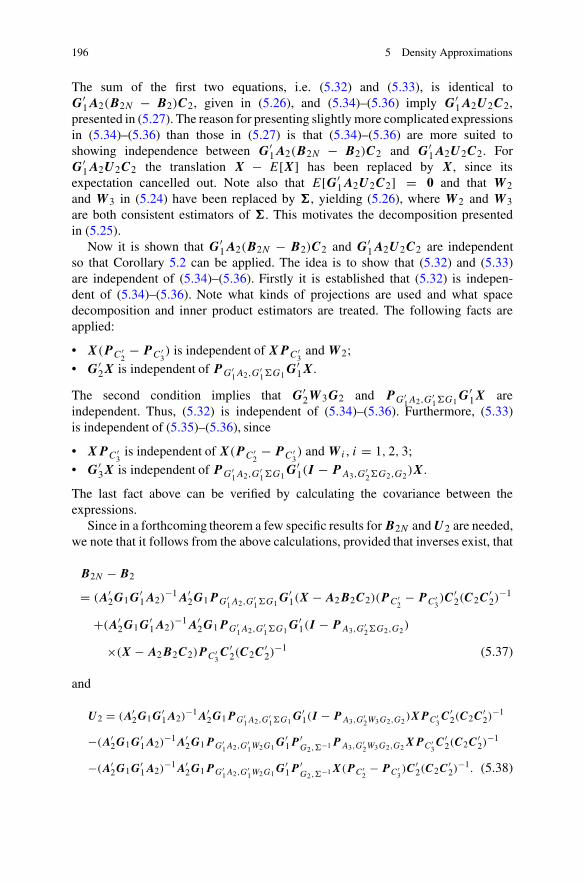
196 5 Density Approximations
The sum of the first two equations, i.e. (5.32) and (5.33), is identical toG′
1A2(B2N − B2)C2, given in (5.26), and (5.34)–(5.36) imply G′1A2U2C2,
presented in (5.27). The reason for presenting slightly more complicated expressionsin (5.34)–(5.36) than those in (5.27) is that (5.34)–(5.36) are more suited toshowing independence between G′
1A2(B2N − B2)C2 and G′1A2U 2C2. For
G′1A2U2C2 the translation X − E[X] has been replaced by X, since its
expectation cancelled out. Note also that E[G′1A2U2C2] = 0 and that W 2
and W 3 in (5.24) have been replaced by �, yielding (5.26), where W 2 and W 3are both consistent estimators of �. This motivates the decomposition presentedin (5.25).
Now it is shown that G′1A2(B2N − B2)C2 and G′
1A2U2C2 are independentso that Corollary 5.2 can be applied. The idea is to show that (5.32) and (5.33)are independent of (5.34)–(5.36). Firstly it is established that (5.32) is indepen-dent of (5.34)–(5.36). Note what kinds of projections are used and what spacedecomposition and inner product estimators are treated. The following facts areapplied:
• X(PC ′2− P C ′
3) is independent of XP C ′
3and W 2;
• G′2X is independent of P G′
1A2,G′1G1
G′1X.
The second condition implies that G′2W 3G2 and PG′
1A2,G′1G1
G′1X are
independent. Thus, (5.32) is independent of (5.34)–(5.36). Furthermore, (5.33)is independent of (5.35)–(5.36), since
• XP C ′3
is independent of X(P C ′2− P C ′
3) and W i , i = 1, 2, 3;
• G′3X is independent of P G′
1A2,G′1G1
G′1(I − PA3,G
′2G2,G2
)X.
The last fact above can be verified by calculating the covariance between theexpressions.
Since in a forthcoming theorem a few specific results for B2N and U 2 are needed,we note that it follows from the above calculations, provided that inverses exist, that
B2N − B2
= (A′2G1G
′1A2)
−1A′2G1PG′
1A2,G′1G1
G′1(X − A2B2C2)(P C′
2− P C′
3)C′
2(C2C′2)
−1
+(A′2G1G
′1A2)
−1A′2G1PG′
1A2,G′1G1
G′1(I − P A3,G
′2G2,G2
)
×(X − A2B2C2)PC′3C′
2(C2C′2)
−1 (5.37)
and
U2 = (A′2G1G
′1A2)
−1A′2G1PG′
1A2,G′1G1
G′1(I − P A3,G
′2W3G2,G2
)XPC′3C′
2(C2C′2)
−1
−(A′2G1G
′1A2)
−1A′2G1PG′
1A2,G′1W2G1
G′1P
′G2,−1P A3,G
′2W3G2,G2
XPC′3C′
2(C2C′2)
−1
−(A′2G1G
′1A2)
−1A′2G1PG′
1A2,G′1W2G1
G′1P
′G2,−1X(PC′
2− PC′
3)C′
2(C2C′2)
−1. (5.38)

5.4 Density Approximation for the Mean Parameter Estimators in the EBRM3B 197
In the Edgeworth-type expansion, D[B2N ] is also needed. Since X(P C ′2− P C ′
3)
and XP C ′3
are independently distributed,
D[B2N ]= (C2C
′2)
−1C2(I − PC′3)C ′
2(C2C′2)
−1 ⊗ (A′2G1(G
′1�G1)
−1G′1A2)
−1
+(C2C′2)
−1C2PC′3C′
2(C2C′2)
−1 ⊗{
(A′2G1(G
′1�G1)
−1G′1A2)
−1
+(A′2G1(G
′1�G1)
−1G′1A2)
−1
×A′2G1(G
′1�G1)
−1G′1A3(A
′3G2(G
′2�G2)
−1G′2A3)
−A′3G1(G
′1�G1)
−1G′1A2
×(A′2G1(G
′1�G1)
−1G′1A2)
−1}
. (5.39)
Although B2N is normally distributed, it does not follow a matrix normal distribu-tion, and as a consequence the inverse of D[B2N ] can be difficult to express in aconvenient way. However, from a computational point of view it can be shown thatD[B2N ]−1 is not too difficult to obtain and the result is indeed applicable. UsingCorollary 5.2 the next theorem can be stated.
Theorem 5.8 Let B2, B2N and U 2 be defined by (5.25), (5.37) and (5.38),respectively. Then an Edgeworth-type expansion of the density of B2 equals
fB2
(Bo) = fB2E(Bo) + r
3 ,
where
fB2E(Bo)= (1 − 1
2 tr{D[B2]D[B2N ]−1 − I })fB2N(Bo)
+ 12 tr{(D[B2]D[B2N ]−1 − I )vec(Bo − B2)vec′(Bo − B2)D[B2N ]−1}fB2N
(Bo);
D[B2] and D[B2N ] are given in Theorem 4.17 (ii) and (5.39), respectively, and
|r 3 | ≤ c
n2 ,
for some fixed constant c which depends on the design matrices.
It can be noted that the approximating density is not a density where a matrixKotz-type distribution is included. In fact the density does not even belong to theclass of matrix elliptical distributions. From an interpretation point of view, this isslightly unfortunate. To obtain a better and more understandable approximation, thenext step is to approximate D[B2] with an error which is proportional to n−2, sothat the overall error of the density approximation will be of the same size as |r
3 |,given in Theorem 5.8.

198 5 Density Approximations
The dispersion matrix D[B2] was presented in Theorem 4.17 (ii), and since c2 −1 = O(n−1) and
n − r(C3) − 1
n − r(C3) − m3 − 1− (1 + c2
m3
n − r(C3) − m3 − 1) = O(n−2),
an approximative dispersion equals
˜D[B2] = s1(C2C′2)
−1C2(I − P C ′3)C′
2(C2C′2)
−1 ⊗ H 1
+ s2(C2C′2)
−1C2P C ′3C′
2(C2C′2)
−1 ⊗ H 2,
where, if n − r(C1) − m1 + q2 − 1 > 0 and n − r(C3) − m3 − 1 > 0,
s1 = n − k2 − 1
n − r(C1) − m1 + q2 − 1, s2 = n − r(C3) − 1
n − r(C3) − m3 − 1, (5.40)
H 1 = (A′2G1(G
′1�G1)
−1G′1A2)
−1 = (A′2A
o1(A
o′1 �Ao
1)−1Ao′
1 A2)−1, (5.41)
H 2 = (A′2G1(G
′1A3)
o((G′1A3)
o′G′
1�G1(G′1A3)
o)−(G′1A3)
o′G′
1A2)−1
= (A′2(A1 : A3)
o((A1 : A3)o′�(A1 : A3)
o)−(A1 : A3)o′A2)
−1. (5.42)
The matrix H 2 is obtained because
H 2 = H 1
+H 1A′2G1(G
′1�G1)
−1G′1A3(A
′3G2(G
′2�G2)
−1G′2A3)
−A′3G1(G
′1�G1)
−1G′1A2H 1
= (I q2 : 0){(A2 : A3)′G1(G
′1�G1)
−1G′1(A2 : A3)}−1(I q2 : 0)′.
Moreover, D[B2N ], given in (5.39), equals
D[B2N ] = (C2C′2)
−1C2(I − P C ′3)C′
2(C2C′2)
−1 ⊗ H 1
+ (C2C′2)
−1C2PC ′3C′
2(C2C′2)
−1 ⊗ H 2.
Hence, ˜D[BN ] and D[B2N ] are of the same form, which helps when exploiting anEdgeworth-type expansion. It follows from Theorem 5.8 that
tr{˜D[B2]D[B2N ]−1 − I } (5.43)
and
tr{(˜D[B2]D[B2N ]−1 − I )vec(Bo − B2)vec′(Bo − B2)D[B2N ]−1} (5.44)

5.4 Density Approximation for the Mean Parameter Estimators in the EBRM3B 199
are of interest. To facilitate calculations, based on the decomposition C(C′2) =
C(C′3)�C(C′
2)∩C(C′3)
⊥, the following non-singular matrix is used, where, withoutany loss of generality, it is assumed that the symmetric square roots exist:
M ′2 = (
C2C′3(C3C
′3)
−1/2 : C2C′2(C2C
′3)
o{(C2C′3)
o′C2C
′2(C2C
′3)
o}−1/2).
(5.45)
To be more explicit about the space decomposition and (5.45), note that (applyingAppendix B, Theorem B.3 (v))
C(C′2(C2C
′3)
o{(C2C′3)
o′C2C
′2(C2C
′3)
o}−(C2C′3)
o′C2) = C(C′
2) ∩ C(C′3)
⊥.
The pre-multiplication by C2 inside M ′2 is only needed for technical reasons, which
can be seen from the next two equations:
M2(C2C′2)
−1C2(I − PC ′3)C′
2(C2C′2)
−1M ′2 =
(
0 00 I r1
)
, r1 = k2 − r(C3),
(5.46)
M2(C2C′2)
−1C2P C ′3C′
2(C2C′2)
−1M ′2 =
(
I r2 00 0
)
, r2 = r(C3). (5.47)
Now (5.43) and (5.44) equal
tr{˜D[B2M′2]D[B2NM ′
2]−1 − I } = q2(r1(s1 − 1) + r2(s2 − 1))
and
tr{(˜D[B2M′2]D[B2NM ′
2]−1 − I )vec((Bo−B2)M′2)vec′((Bo−B2)M
′2)D[B2NM ′
2]−1}= (s2 − 1)tr{H−1
2 (Bo − B2)C′2PC′
3C2(Bo − B2)
′}+(s1 − 1)tr{H−1
1 (Bo − B2)C2C′2(C2C
′3)
o{(C2C′3)
o′C2C
′2(C2C
′3)
o}−1
×(C2C′3)
o′C2C
′2(Bo − B2)
′},
where s1 and s2 are given in (5.40). Hence, applying Theorem 5.8 and the abovecalculations then lead to the next theorem which has quite an easily interpretablestructure. Furthermore, s1 − 1 and s2 − 1 are both O(n−1).
Theorem 5.9 Let B2 and B2N be defined by (5.25) and (5.37), respectively. AnEdgeworth-type expansion of the density of B2 equals
fB2
(Bo) = f˜B2E
(Bo) + r 3 ,

200 5 Density Approximations
where
f˜B2E
(Bo) = (1 − 12q2(r1(s1 − 1) + r2(s2 − 1))fB2N (Bo)
+ 12 (s2 − 1)tr{H−1
2 (Bo − B2)C′2P C ′
3C2(Bo − B2)
′}fB2N(Bo)
+ 12 (s1 − 1)tr{H−1
1 (Bo − B2)C2(I − P C ′3)C′
2(Bo − B2)′}fB2N
(Bo);
ri, si ,H i , i = 1, 2, are given by (5.46), (5.47) and (5.40)–(5.42), and
|r 3 | ≤ c
n2,
for some fixed constant c which depends on the design matrices. The density fB2N
can be factorized as
fB2N(Bo) = |C2C
′2|q2/2fB2N2C2(BoC2)fB2N1C2(BoC2),
where fB2N1C2(BoC2) and fB2N2C2(BoC2) are density representations for
B2N1C2 = (A′2G1(G
′1�G1)
−1G′1A2)
−1A′2G1(G
′1�G1)
−1G′1X(PC ′
2− PC ′
3)
∼ Nq2,n(B2C2(I − PC ′3),H 1,P C ′
2− P C ′
3)
within X(PC ′2− PC ′
3) and
B2N2C2
= (A′2G1(G
′1�G1)
−1G′1A2)
−1A′2G1(G
′1�G1)
−1G′1(I − PA3,G′
2G2,G2)XP C′
3
∼ Nq2,n(B2C2PC′3,H 2,PC′
3)
within XPC ′3, respectively. Moreover, B2N = B2N1 + B2N2 .
Proof From Theorem 5.8 it follows that the only detail which remains to be provenis
fB2N= |C2C
′2|q2/2fB2N2C2(BoC2)fB2N1C2(BoC2).
Now, if using M2, given by (5.45), then
fB2N(Bo) ∝ |D[B2N ]|−1/2e
− 12 tr{D[B2N ]−1vec(Bo−B2)vec′(Bo−B2)}
= |C2C′2|q2/2|D[B2NM ′
2]|−1/2e− 1
2 tr{D[B2N M ′2]−1vec((Bo−B2)M ′
2)vec′((Bo−B2)M′2)}
= |C2C′2|q2/2fB2N2 C2(BoC2)fB2N1 C2(BoC2).
��

5.4 Density Approximation for the Mean Parameter Estimators in the EBRM3B 201
The density factorization in Theorem 5.9 was presented in order to give some insightinto the structure of the Edgeworth-type expansion. The expression B2NiC2, i =1, 2, was included in the density functions, but this does not mean that a true variablesubstitution has taken place, which explains why no Jacobians were included inthe expressions. Moreover, the densities fB2N1C2(BoC2) and fB2N2C2(BoC2) arerepresentations of densities for normally distributed random variables with singulardistributions; i.e. the expressions can only be considered to be real densities onappropriate subspaces.
Finally, B1 is considered, which is more difficult than B2 and B3, because B1 is afunction of both B2 and B3. However, the approach to obtaining results concerninga density approximation for B1 will follow the same procedure as that used whenobtaining Theorems 5.8 and 5.9. Let us restate A1B1C1 as given in (4.137):
A1(B1 − B1)C1
= P A1,W1(X − E[X])(P C′1− PC′
2)
+PA1,W1(I − PA2,G′1W2G1,G1
)(X − E[X])(P C′2− PC′
3)
+PA1,W1(I − PA2,G′1W2G1,G1
)(I − P A3,G′2W3G2,G2
)(X − E[X])P C′3.
(5.48)
Similar to the treatment for B3 and B2, the estimator A1B1C1 is split into anormally distributed variable and a symmetrically distributed error term A1U1C1with mean 0, i.e.
A1(B1 − B1)C1 = A1(B1N − B1)C1 − A1U 1C1, (5.49)
where A1B1NC1 is a matrix obtained from A1B1C1 when W i , i = 1, 2, 3, isreplaced by �, i.e.
A1(B1N − B1)C1 = PA1,(X − E[X])(P C ′1− PC ′
2) (5.50)
+P A1,(I − PA2,G′1G1,G1
)(X − E[X])(P C ′2− PC ′
3) (5.51)
+P A1,(I − PA2,G′1G1,G1
)(I − PA3,G′2G2,G2
)(X − E[X])PC ′3,
(5.52)
and B1N − B1 = (A′1A1)
−1A′1A1(B1N − B1)C1C
′1(C1C
′1)
−1. The threeterms, (5.50)–(5.52), in A1B1NC1 are independent since X(P C ′
1− P C ′
2),
X(P C ′2− P C ′
3) and XPC ′
3are independently distributed. Therefore,
D[B1N ] = (C1C′1)
−1C1(I − P C ′2) ⊗ (A′
1�−1A1)
−1
+(C1C′1)
−1C′1(P C ′
2− PC ′
3)C′
1(C1C′1)
−1

202 5 Density Approximations
⊗{(A′1�
−1A1)−1 + F 2A2(A
′2G1(G
′1�G1)
−1G′1A2)
−A′2F
′2}
+(C1C′1)
−1C′1P C ′
3C′
1(C1C′1)
−1
⊗{
(A′1�
−1A1)−1 + F 2A2(A
′2G1(G
′1�G1)
−1G′1A2)
−A′2F
′2
+F 3A3(A′3G2(G
′2�G2)
−1G′2A3)
−A′3F
′3
}
, (5.53)
where F 2 and F 3 are given by (4.144) and (4.145), respectively. Moreover, it isobvious that E[A1B1NC1] = A1B1C1. Now A1U 1C1 is studied. After somecalculations it follows from (5.48) and (5.50)–(5.52) that the “error” term A1U1C1in (5.49) equals
A1U1C1 = −PA1,W1P′G1,−1X(P C ′
1− P C ′
2) (5.54)
−PA1,W1P′G1,
−1(I − PA2,G′1W2G1,G1
)X(P C ′2− P C ′
3) (5.55)
+PA1,P A2,G′1W2G1,G1
P ′G2,−1X(P C ′
2− P C ′
3) (5.56)
−PA1,W1P′G1,−1(I − PA2,G′
1W2G1,G1)(I − P A3,G
′2W3G2,G2
)XPC ′3
(5.57)
+PA1,P A2,G′1W2G1,G1
P ′G2,
−1(I − P A3,G′2W3G2,G2
)XP C ′3
(5.58)
+PA1,(I − PA2,G′1G1,G1
)P A3,G′2W3G2,G2
P ′G3,−1XPC ′
3, (5.59)
and U 1 = (A′1A1)
−1A′1A1U 1C1C
′1(C1C
′1)
−1. Next the independence betweenA1B1NC1 and A1U 1C1 is established. First it is shown that the right-hand sideof (5.50) is independent of (5.54)–(5.59) and thereafter that (5.51) is independentof (5.54)–(5.59), and finally it is established that (5.52) is independent of (5.54)–(5.59).
The expression in (5.50) is independent of (5.54)–(5.59), since
• X(PC ′1− P C ′
2) is independent of W 1 and XP C ′
3;
• P A1,X is independent of (I − P A1,)X and G′iX, i = 1, 2, 3, as well as
G′1W 2G1 and G′
2W 3G2.
Moreover, the expression in (5.51) is independent of (5.54)–(5.59), since
• X(PC ′2− P C ′
3) is independent of W 1, W 2, X(P C ′
1− P C ′
2) and XP C ′
3;
• P A1,(I − P A2,G′1G1,G1
)X is independent of G′2X and G′
2W 3G2.
Furthermore, the expression in (5.52) is independent of (5.54)–(5.59), since
• XP C ′3
is independent of W i , i = 1, 2, 3, X(P C ′1− P C ′
2) and X(PC ′
2− PC ′
3);
• P A3,G′2G2,G2
X is independent of G′3X.
Hence, Corollary 5.2 can be applied and the following theorem, correspondingto Theorem 5.9 for B2, has been verified.

5.4 Density Approximation for the Mean Parameter Estimators in the EBRM3B 203
Theorem 5.10 Let B1, B1N and U1 be defined via (5.48), (5.50)–(5.52)and (5.54)–(5.59), respectively. Then an Edgeworth-type expansion of the densityof B1 equals
fB1
(Bo) = fB1E (Bo) + r 3 ,
where
fB1E(Bo)=(1 − 1
2 tr{D[B1]D[B1N ]−1 − I })fB1N(Bo)
+ 12 tr{(D[B1]D[B1N ]−1 − I )vec(Bo − B1)vec′(Bo − B1)D[B1N ]−1}fB1N (Bo);
D[B1] and D[B1N ] are given in Theorem 4.17 (iii) and (5.53), respectively, and
|r 3 | ≤ c
n2 ,
for some fixed constant c which depends on the design matrices.
As for B2, in order to obtain a more understandable approximation, the nextstep is to approximate D[B1] with an error which is proportional to n−2. FromD[B1] in Theorem 4.17 (iii) it follows, by performing some calculations, that anapproximative dispersion equals
˜D[B1] = s3(C1C′1)
−1C1(I − P C ′2)C′
1(C1C′1)
−1 ⊗ (A′1�
−1A1)−1
+ s4(C1C′1)
−1C1(P C ′2− P C ′
3)C′
1(C1C′1)
−1 ⊗ {
(A′1�
−1A1)−1
+ F 2A2(A′2G1(G
′1�G1)
−1G′1A2)
−A′2F
′2
}
+ (C1C′1)
−1C1P C ′3C′
1(C1C′1)
−1 ⊗{
s2{
(A′1�
−1A1)−1
+ F 3A3(A′3G2(G
′2�G2)
−1G′2A3)
−A′3F
′3
}
+ F 2A2(A′2G1(G
′1�G1)
−1G′1A2)
−A′2F
′2
}
,
where
s3 = n − k1 − 1
n − r(C1) − p + q1 − 1, s4 = n − r(C2) − 1
n − r(C2) − m2 − 1(5.60)
and s2 is given in (5.40). Hence,
˜D[B1] − D[B1N ] = (s3 − 1)(C1C′1)
−1C1(I − P C′2)C ′
1(C1C′1)
−1 ⊗ (A′1�
−1A1)−1
+ (s4 − 1)(C1C′1)
−1C1(P C′2− P C′
3)C′
1(C1C′1)
−1 ⊗ {
(A′1�
−1A1)−1
+ F 2A2(A′2G1(G
′1�G1)
−1G′1A2)
−A′2F
′2
}

204 5 Density Approximations
+ (s2 − 1)(C1C′1)
−1C1P C′3C ′
1(C1C′1)
−1 ⊗ {
(A′1�
−1A1)−1
+ F 3A3(A′3G2(G
′2�G2)
−1G′2A3)
−A′3F
′3
}
. (5.61)
The constants si − 1, i = 2, 3, 4, are all O(n−1).When discussing B2, the calculations were simplified by introducing the matrix
M2 in (5.45). Now, when considering B1, the same technique is applied, but insteadof M2, the matrix
M ′1 = (
C1C′3(C3C
′3)
−1/2 : C1C′2(C2C
′3)
o{(C2C′3)
o′C2C
′2(C2C
′3)
o}−1/2
: C1C′1(C1C
′2)
o{(C1C′2)
o′C1C
′1(C1C
′2)
o}−1/2) (5.62)
is used. The matrix is created according to the decomposition
C(C′1) = C(C′
3) � C(C′2) ∩ C(C′
3)⊥ � C(C′
1) ∩ C(C′2)
⊥.
Then, (diag(•, •, •) denotes the block-diagonal operator, see Appendix A, Sect. A.6)
M1(C1C′1)
−1C1(I − P C ′2)C ′
1(C1C′1)
−1M ′1 = diag(0, 0, I r1), r1 = k1 − r(C2),
(5.63)
M1(C1C′1)
−1C1(P C ′2− PC ′
3)C ′
1(C1C′1)
−1M ′1 = diag(0, I r20, ),
r2 = r(C2) − r(C3), (5.64)
M1(C1C′1)
−1C1P C ′3C ′
1(C1C′1)
−1M ′1 = diag(I r3, 0, 0), r3 = r(C3), (5.65)
and applying (5.61)
˜D[B1M′1] − D[B1NM ′
1] = (s3 − 1)diag(0, 0, I r1) ⊗ (A′1�
−1A1)−1
+ (s4 − 1)diag(0, I r2 , 0) ⊗ {(A′1�
−1A1)−1 + F 2A2(A
′2G1(G
′1�G1)
−1G′1A2)
−A′2F
′2}
+ (s2 − 1)diag(I r3 , 0, 0) ⊗ {(A′1�
−1A1)−1 + F 3A3(A
′3G2(G
′2�G2)
−1G′2A3)
−A′3F
′3}.
(5.66)
Moreover, according to Corollary 5.2 the following two expressions are needed:
tr{(˜D[B1] − D[B1N ])D[B1N ]−1} (5.67)
and
tr{(˜D[B1] − D[B1N ])D[B1N ]−1vec(Bo − B1)vec′(Bo − B1)D[B1N ]−1}.(5.68)

5.4 Density Approximation for the Mean Parameter Estimators in the EBRM3B 205
Explicit calculations of (5.67) and (5.68) are left to the reader. Here it is noted thatall calculations become straightforward if one uses the matrix M1, given in (5.62),since
tr{(˜D[B1] − D[B1N ])D[B1N ]−1}= tr{(˜D[B1M
′1] − D[B1NM ′
1])D[B1NM ′1]−1}
and
tr{(˜D[B1] − D[B1N ])D[B1N ]−1vec(Bo − B1)vec′(Bo − B1)D[B1N ]−1}= tr
{
(˜D[B1M′1] − D[B1NM ′
1])D[B1NM ′1]−1
×vec((Bo − B1)M′1)vec′((Bo − B1)M
′1)D[B1NM ′
1]−1}
.
Among other things, (5.66) presents ˜D[B1M′1] − D[B1NM ′
1], and
D[B1NM ′1]−1
= diag(0, 0, I r1) ⊗ A′1�
−1A1 + diag(0, I r2 , 0) ⊗ H−13 + diag(I r3 , 0, 0) ⊗ H−1
4 ,
where
H 3 = (I : 0)((A1 : A2)′�−1(A1 : A2))
−1(I : 0)′= (A′
1�−1A1)
−1 + F 2A2(A′2G1(G
′1�G1)
−1G′1A2)
−A′2F
′2 (5.69)
and
H 4 = (I : 0 : 0)((A1 : A2 : A3)′�−1(A1 : A2 : A3))
−1(I : 0 : 0)′
= (A′1�
−1A1)−1 +
2∑
i=1
F i+1Ai+1(A′i+1Gi (G
′i�Gi )
−1G′iAi+1)
−A′i+1F
′i+1.
(5.70)
Moreover, let
H 5 = (A′1�
−1A1)−1 + F 3A3(A
′3G2(G
′2�G2)
−1G′2A3)
−A′3F
′3. (5.71)
Theorem 5.11 Let B1 and B1N be defined in (5.48) and (5.50)–(5.52). Then anEdgeworth-type expansion of the density of B1, assuming that all the constantsgiven below exist, equals
fB1
(Bo) = f˜B1E
(Bo) + r 3 ,

206 5 Density Approximations
where
f˜B1E
(Bo) = (1 − 12 (q1(r1(s3 − 1) + r2(s4 − 1)) + (s2 − 1)tr{H 5H
−14 })fB1N (Bo)
+ 12 (s3 − 1)tr{(A′
1�−1A1)
−1(Bo − B1)C′1(I − P C2)C1(Bo − B1)
′}fB1N (Bo)
+ 12 (s4 − 1)tr{H−1
3 (Bo − B1)C1(P C′2− PC′
3)C′
1(Bo − B1)′}fB1N
(Bo)
+ 12 (s2 − 1)tr{H−1
4 H 5H−14 (Bo − B1)C1PC′
3C′
1(Bo − B1)′}fB1N
(Bo);
ri , i = 1, 2, 3, are defined in (5.63)–(5.65), si , i = 2, 3, 4, in (5.40) and (5.60), andH i , i = 3, 4, 5, in (5.69)–(5.71), and
|r 3 | ≤ c
n2 ,
for some fixed constant c which depends on the design matrices. The density fB1N
can be factorized as
fB1N(Bo) = |C1C
′1|q1/2fB1N3 C1(BoC1)fB1N2 C1(BoC1)fB1N1 C1(BoC1),
where fB1NiC2(BoC2), i = 1, 2, 3, are density representations for
B1N1C1 = (A′1�
−1A1)−1A′
1�−1X(P C ′
1− P C ′
2)
∼ Nq1,n(B1C1(I − P C ′2), (A′
1�−1A1)
−1,P C ′1− PC ′
2)
within X(PC ′1− PC ′
2),
B1N2C1 = (A′1�
−1A1)−1A′
1�−1(I − P A2,G
′1G1,G1
)X(P C ′2− P C ′
3)
∼ Nq1,n(B1C1(P C ′2− P C ′
3),H 3,P C ′
2− PC ′
3)
within X(PC ′2− PC ′
3), and
B1N3C1 = (A′1�
−1A1)−1A′
1�−1(I − P A2,G
′1G1,G1
)(I − PA3,G′2G2,G2
)XP C ′3
∼ Nq1,n(B1C1PC ′3,H 4,P C ′
3)
within XPC ′3, respectively. Moreover, B1N = B1N1 + B1N2 + B1N3 .
5.5 Density Approximation for the Mean ParameterEstimators in the EBRM3
W
The ideas presented below are the same as those used when working with theEBRM3
B in the previous Sect. 5.4. In correspondence with Sect. 5.4, it will beshown that the distributions of the estimators B i , i = 1, 2, 3, for the EBRM3
W ,can all be decomposed into a normally distributed part and an error term which has

5.5 Density Approximation for the Mean Parameter Estimators in the EBRM3W 207
an expectation equal to 0 and is independent of the normal part. Indeed, from a linearmodel point of view (e.g. see Exercise 1.3, p. 308 in Rao, 1973), the decompositionsare both natural and interpretable.
Starting with B3, given in Theorem 3.3, it follows that under full rank conditions
B3 = B3N − U 3,
where
B3N = (A′3�
−1A3)−1A′
3�−1XQ2C
′3(C3Q2C
′3)
−1, (5.72)
U 3 = −(A′3S
−11 A3)
−1A′3S
−11 (I − P A3,)XQ2C
′3(C3Q2C
′3)
−1. (5.73)
Since S1 is independent of XQ2C′3 and (I −P A3,)X is independent of A′
3�−1X,
the two matrices B3N and U are independently distributed. Moreover,
D[B3N ] = (C3Q2C′3)
−1 ⊗ (A′3�
−1A3)−1 (5.74)
and, if n − r(C′1 : C′
2 : C′3) − p + q3 − 1 > 0 (see Theorem 4.25 (i)),
D[B3] = (1 + s1)(C3Q2C′3)
−1 ⊗ (A′3�
−1A3)−1, (5.75)
where
s1 = p−q3n−r(C ′
1:C ′2:C ′
3)−p+q3−1 . (5.76)
Hence, correspondingly to Theorem 5.7, we can present the next theorem, omittinga proof of the statement concerning the error term.
Theorem 5.12 Let B3,B3N andU 3 (u3 = vecU3) be given by Theorem 3.3, (5.72)and (5.73), respectively. Then an Edgeworth-type expansion of the density of B3equals
fB3
(Bo) = fB3E(Bo) + r
3 ,
where
fB3E (Bo) = fB3N (Bo) + 12E[(u′
3)⊗2]vecf 2
B3N(Bo)
= (1 − 12 s1k3q3 + 1
2 s1 tr{A′3�
−1A3(Bo − B3)C3Q2C′3(Bo − B3)
′})fB3N(Bo),
with s1 defined in (5.76) and supposed to exist, and
|r 3 | ≤ c
n2 ,
for some fixed constant c which is a function of the design matrices.

208 5 Density Approximations
In Theorem 5.12 the density corresponds to a mixture of a Kotz-type distribution(see Appendix A, Sect. A.10) and a normal distribution.
For B2, given in Theorem 3.3, the following decomposition holds under somefull rank conditions. Let F 2 = (A′
2A2)−1A′
2, then
B2 = F 2P A2,S2XQ1C
′2(C2Q1C
′2)
−1
−F 2P A3,S1XQ2C′3(C3Q2C
′3)
−C3Q1C′2(C2Q1C
′2)
−1, (5.77)
B2N = F 2P A2,XQ1C′2(C2Q1C
′2)
−1 (5.78)
−F 2P A3,XQ2C′3(C3Q2C
′3)
−C3Q1C′2(C2Q1C
′2)
−1, (5.79)
U2 = −F 2P A2,S2(I − PA2,)XQ1C
′2(C2Q1C
′2)
−1
+F 2P A3,S1(I − PA3,)XQ2C′3(C3Q2C
′3)
−C3Q1C′2(C2Q1C
′2)
−1,
(5.80)
and
B2 = B2N − U2.
As before, the independence between B2N and U2 has to be proven. Note thatXQ1C
′2 is independent of S1, S2 and XQ2C
′3, and P A2,X is independent of
(I −PA2,)X. Hence, the expression on the right-hand side of (5.78) is independentof U 2. Moreover, XQ2C
′3 is independent of S1 and PA3,XQ2C
′3 is independent
of S2, (I − P A2,)X and (I − PA3,)X. Therefore, (5.79) is independent of U2,implying independence between B2N and U 2.
Concerning moments, E[U2] = 0,
D[B2N ] = (C2Q1C′2)
−1 ⊗ (A′2�
−1A2)−1
+(C2Q1C′2)
−1C2Q1C′3(C3Q2C
′3)
−C3Q1C′2(C2Q1C
′2)
−1
⊗F 2A3(A′3�
−1A3)−A′
3F′2, (5.81)
and according to Theorem 4.25 (ii)
D[B2] = (C2Q1C′2)
−1 ⊗{
(1 + c1)(A′2�
−1A2)−1
+c1(c2 − 1)F 2A3(A′3�
−1A3)−A′
3F′2
}
+(1 + c3)(C2Q1C′2)
−1C2Q1C′3(C3Q2C
′3)
−C3Q1C′2(C2Q1C
′2)
−1
⊗F 2A3(A′3�
−1A3)−A′
3F′2, (5.82)

5.5 Density Approximation for the Mean Parameter Estimators in the EBRM3W 209
where
c1 = p−q2n−r(C′
1:C ′2)−p+q2−1 , c2 = n−r(C′
1:C ′2)−p+r(A3)−1
n−r(C′1:C ′
2:C ′3)−p+r(A3)−1 , (5.83)
c3 = p−r(A3)
n−r(C′1:C ′
2:C ′3)−p+r(A3)−1 , (5.84)
and all three constants are supposed to be positive and finite.
Theorem 5.13 Let B2, B2N and U 2 be defined by (5.77)–(5.80). Then anEdgeworth-type expansion of the density of B2 equals
fB2
(Bo) = fB2E(Bo) + r
3 ,
where
fB2E (Bo) = (1 − 12 tr{D[B2]D[B2N ]−1 − I })fB2N (Bo)
+ 12 tr{(D[B2]D[B2N ]−1 − I )vec(Bo − B2)vec′(Bo − B2)D[B2N ]−1}fB2N (Bo);
D[B2] and D[B2N ] are supposed to exist and are presented in (5.82) and (5.81),respectively, and
|r 3 | ≤ c
n2 ,
for some fixed constant c which depends on the design matrices.
Noting that c1(c2 − 1) = O(n−2), it immediately follows that a naturalapproximation of D[B2] in (5.82) is given by
˜D[B2] = (1 + c1)(C2Q1C′2)
−1 ⊗ (A′2�
−1A2)−1
+(1 + c3)(C2Q1C′2)
−1C2Q1C′3(C3Q2C
′3)
−C3Q1C′2(C2Q1C
′2)
−1
⊗F 2A3(A′3�
−1A3)−A′
3F′2. (5.85)
Moreover, to simplify calculations, a matrix M2 is introduced which corresponds tothe matrix given in (5.45):
M ′2 = (
A′2�
−1A3(A′3�
−1A3)−1/2 : A′
2�−1A2(A
′2�
−1A3)o
×{(A′2�
−1A3)o′A′
2�−1A2(A
′2�
−1A3)o}−1/2),
where, without any loss of generality, the square roots are supposed to exist; i.e. ithas to be supposed that A3 is of full rank, which we can always assume to holdin (5.82) and (5.85). Then
˜D[M2B2] − D[M2B2N ] = c1H 1 ⊗ I q2 + c3H 3 ⊗ diag(I r(A3), 0),

210 5 Density Approximations
where
H 1 = (C2Q1C′2)
−1, (5.86)
H 3 = (C2Q1C′2)
−1C2Q1C′3(C3Q2C
′3)
−C3Q1C′2(C2Q1C
′2)
−1. (5.87)
Moreover, let
H 2 = H 1 + H 3 = (I : 0)((C′2 : C′
3)′Q1(C
′2 : C′
3))−1(I : 0)′. (5.88)
Then
D[M2B2N ]−1 = H−11 ⊗ diag(0, I q2−r(A3)) + H−1
2 ⊗ diag(I r(A3), 0)
and
D[M2B2N ]−1vec(M2(B2N − B2))
= vec{
{(A′2�
−1A3)o′A′
2�−1A2(A
′2�
−1A3)o}−1/2
×(A′2�
−1A3)o′A′
2�−1A2(B2N − B2)H
−11
}
+vec{(A′3�
−1A3)−1/2A′
3�−1A2(B2N − B2)H
−12 }.
Theorem 5.14 Let B2 and B2N be defined by (5.77)–(5.80). Then an Edgeworth-type expansion of the density of B2 equals
fB2
(Bo) = f˜B2E
(Bo) + r 3 ,
where
f˜B2E
(Bo)
= (1 − 12 (q2 − r(A3))k2c1 − 1
2 c1r(A3)tr{H 1H−12 } − 1
2 c3r(A3)tr{H 3H−12 })fB2N
(Bo)
+ 12 c1tr{H−1
1 (Bo − B2)′A′
2Ao3(A
o′3 �Ao
3)−Ao′
3 A2(Bo − B2)}fB2N(Bo)
+ 12 c1tr{H−1
2 H 1H−12 (Bo − B2)
′A′2�
−1P A3,A2(Bo − B2)}fB2N(Bo)
+ 12 c3tr{H−1
2 H 3H−12 (Bo − B2)
′A′2�
−1P A3,A2(Bo − B2)}fB2N(Bo),
where c1 and c3 are supposed to exist and are given by (5.83) and (5.84),respectively, and H i , i = 1, 2, 3, are given by (5.86)–(5.88). Furthermore,
|r 3 | ≤ c
n2,

5.5 Density Approximation for the Mean Parameter Estimators in the EBRM3W 211
for some fixed constant c which depends on the design matrices. The density fB2N
can be factorized as
fB2N (Bo) = |A′2�
−1A2|k2/2fA2B2N2(A2Bo)fA2B2N1
(A2Bo),
where fA2B2N1(A2Bo) and fA2B2N2
(A2Bo) are density representations for
A2B2N1 = (P A2, − PA3,)XQ1C′2(C2Q1C
′2)
−1
∼ Np,k2((I − P A3,)A2B2, (P A2, − P A3,)�,H 1)
within (P A2, − P A3,)X and
A2B2N2 = P A3,X(I − Q2C′3(C3Q2C
′3)
−C3)Q1C′2(C2Q1C
′2)
−1
∼ Np,q2(P A3,A2B2,P A3,�,H 2)
within P A3,X, respectively. Moreover, B2N = B2N1 + B2N2 .
Finally, B1 is discussed briefly. The results are obtained using a procedure similarto that presented earlier. Now Theorem 3.3, together with a number of calculations,yields
B1 = B1N − U 1,
where
B1N = F 1PA1,XC′1(C1C
′1)
−1 (5.89)
−F 1PA2,XQ1C′2(C2Q1C
′2)
−C2C′1(C1C
′1)
−1 (5.90)
−F 1P A3,XQ2C′3(C3Q2C
′3)
−C3(I − Q1C′2(C2Q1C
′2)
−C2)C′1(C1C
′1)
−1, (5.91)
with F 1 = (A′1A1)
−1A′1 and
U1 = −F 1PA1,S3(I − P A1,)XC′
1(C1C′1)
−1
+F 1P A2,S2(I − PA2,)Q1C
′2(C2Q1C
′2)
−C2C′1(C1C
′1)
−1 −+F 1PA3,S1(I−P A3,)XQ2C
′3(C3Q2C
′3)
−C3(I−Q1C′2(C2Q1C
′2)
−C2)C′1(C1C
′1)
−1.
(5.92)
The independence between B1N and U 1 has to be verified. In the right-hand sideof (5.89) the expression is independent of U 1, since
• XC′1 is independent of S3, S2, S1, XQ1, XQ2;
• P A1,XC′1 is independent of (I − P A1,)X.

212 5 Density Approximations
The second term of B1N , given in (5.90), is independent of U 1, since
• XQ′1C
′2 is independent of S2, S1, XQ2;
• P A2,XQ1C′2 is independent of S3, (I − P A2,)X, (I − P A1,)X.
The third term, given in (5.91), is independent of U1, since
• XQ′2C
′3 is independent of S1;
• P A3,XQ2C′3 is independent of S3, S2, (I − P A1,)X, (I − P A2,)X,
(I − P A3,)X.
Thus, B1N and U 1 are independently distributed. Moreover, in order to perform anEdgeworth-type expansion, dispersion matrices are needed, among others D[B1N ],which equals
D[B1N ] = (C1C′1)
−1 ⊗ (A′1�
−1A1)−1
+(C1C′1)
−1C1C′2(C2Q1C
′2)
−C2C′1(C1C
′1)
−1 ⊗ F 1A2(A′2�
−1A2)−A′
2F′1
+(C1C′1)
−1C1(I − C′2(C2Q1C
′2)
−C2Q1)
×C′3(C3Q2C
′3)
−C3(I − Q1C′2(C2Q1C
′2)
−C2)C′1(C1C
′1)
−1
⊗F 1A3(A′3�
−1A3)−A′
3F′1. (5.93)
Theorem 5.15 Let B1, B1N and U 1 be defined by Theorem 3.3, (5.89)–(5.91)and (5.92), respectively. Then an Edgeworth-type expansion of the density of B1equals
fB1
(Bo) = fB1E(Bo) + r
3 ,
where
fB1E (Bo) = (1 − 12 tr{D[B1]D[B1N ]−1 − I })fB1N (Bo)
+ 12 tr{(D[B1]D[B1N ]−1 − I )vec(Bo − B1)vec′(Bo − B1)D[B1N ]−1}fB1N
(Bo);
D[B1] and D[B1N ] are given in Theorem 4.25 (iii) and (5.93), respectively, and
|r 3 | ≤ c
n2 ,
for some fixed constant c which depends on the design matrices.
Now D[B1] is approximated with an error which is proportional to n−1.Using the definition of the constants c1 and d1 presented in Lemma 4.6 (see alsoTheorem 4.25 (iii)), an approximative dispersion equals
˜D[B1] = (1 + d1)(C1C′1)
−1 ⊗ (A′1�
−1A1)−1
+(1 + c1)(C1C′1)
−1C1C′2(C2Q1C
′2)
−C2C′1(C1C
′1)
−1 ⊗ F 1A2(A′2�
−1A2)−A′
2F′1
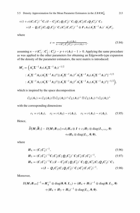
5.5 Density Approximation for the Mean Parameter Estimators in the EBRM3W 213
+(1 + e)(C1C′1)
−1C1(I − C′2(C2Q1C
′2)
−C2Q1)C′3(C3Q2C
′3)
−C3
×(I − Q1C′2(C2Q1C
′2)
−C2)C′1(C1C
′1)
−1 ⊗ F 1A3(A′3�
−1A3)−A′
3F′1,
where
e = p−r(A3)
n−r(C ′1:C ′
2:C ′3)−p+r(A3)−1
, (5.94)
assuming n − r(C′1 : C′
2 : C′3) − p + r(A3) − 1 > 0. Applying the same procedure
as was applied to the other parameters for obtaining an Edgeworth-type expansionof the density of the parameter estimators, the next matrix is introduced:
M ′1 =
(
A′1�
−1A3(A′3�
−1A3)−1/2
: A′1�
−1A2(A′2�
−1A3)o{(A′
2�−1A3)
o′A′
2�−1A2(A
′2�
−1A3)o}−1/2
: A′1�
−1A1(A′1�
−1A2)o{(A′
1�−1A2)
o′A′
1�−1A1(A
′1�
−1A2)o}−1/2
)
,
which is inspired by the space decomposition
C(A1) = C(A3) � C(A2) ∩ C(A3)⊥ � C(A1) ∩ C(A2)
⊥
with the corresponding dimensions
r1 = r(A3), r2 = r(A2) − r(A3), r3 = r(A1) − r(A2). (5.95)
Hence,
˜D[M1B1] − D[M1B1N ]=d1H 4 ⊗ I + c1H 5 ⊗ diag(I r1+r2, 0)
+eH 6 ⊗ diag(I r1, 0, 0),
where
H 4 = (C1C′1)
−1, (5.96)
H 5 = (C1C′1)
−1C1C′2(C2Q1C
′2)
−C2C′1(C1C
′1)
−1, (5.97)
H 6 = (C1C′1)
−1C1(I − C′2(C2Q1C
′2)
−C2Q1)C′3(C3Q2C
′3)
−C3
×(I − Q1C′2(C2Q1C
′2)
−C2)C′1(C1C
′1)
−1. (5.98)
Moreover,
D[M1B1N ]−1 =H−14 ⊗ diag(0, 0, I r3) + (H 4 + H 5)
−1 ⊗ diag(0, I r2, 0)
+(H 4 + H 5 + H 6)−1 ⊗ diag(I r1, 0, 0).

214 5 Density Approximations
With the above-provided definitions and relations the next theorem can be formu-lated.
Theorem 5.16 Let B1 andB1N be defined by Theorem 3.3 and (5.89)–(5.91). Thenan Edgeworth-type expansion of the density of B1 equals
fB1
(Bo) = f˜B1E
(Bo) + r 3 ,
where
f˜B1E
(Bo) = (1 − 12 (d1k1r3 + tr{r2(d1H 4 + c1H 5)(H 4 + H 5)
−1
+r1(d1H 4 + c1H 5 + eH 6)(H 4 + H 5 + H 6)−1})fB1N
(Bo)
+ 12 tr
{
d1H−14 (Bo − B1)
′A′1�
−1A1(A′1�
−1A2)o
×{(A′1�
−1A2)o′A′
1�−1A1(A
′1�
−1A2)o}−1(A′
1�−1A2)
o′A′
1�−1A1(Bo − B1)
}
×fB1N(Bo)
+ 12 tr
{
(H 4 + H 5)−1(d1H 4 + c1H 5)(H 4 + H 5)
−1(Bo − B1)′A′
1�−1A2(A
′2�
−1A3)o
×{(A′2�
−1A3)o′A′
2�−1A2(A
′2�
−1A3)o}−1(A′
2�−1A3)
o′A′
2�−1A1(Bo − B1)
}
×fB1N(Bo)
+ 12 tr
{
(H 4 + H 5 + H 6)−1(d1H 4 + c1H 5 + eH 6)(H 4 + H 5 + H 6)
−1(Bo − B1)′
×A′1�
−1PA3,A1(Bo − B1)}
fB1N(Bo);
ri , i = 1, 2, 3, are defined in (5.95), c1, d1 and e are defined by (5.83), Lemma 4.6and (5.94), respectively, H i , i = 3, 4, 5, are given by (5.96)–(5.98), and
|r 3 | ≤ c
n2 ,
for some fixed constant c which depends on the design matrices. The density fB1N
can be factorized as
fB1N= |A′
1�−1A1|k1/2fA1B1N3
(A1Bo)fA1B1N2(A1Bo)fA1B1N1
(A1Bo),
where fA1B1Ni(A1Bo), i = 1, 2, 3, are density representations for
A1B1N1 = (P A1, − P A2,)XH1/24
∼ Np,k1((I − P A2)A1B1, (P A1, − PA2,)�,H 4)

5.5 Density Approximation for the Mean Parameter Estimators in the EBRM3W 215
within (P A1 − P A2)X,
A1B1N2 = (P A2, − P A3,)X(H 4 + H 5)1/2
∼ Np,k1((PA2, − P A3,)A1B1, (P A2, − P A3,)�,H 4 + H 5)
within (P A2 − P A3)X, and
A1B1N3 = P A3,X(H 4 + H 5 + H 6)1/2
∼ Np,k1(PA3,A1B1,P A3,�,H 4 + H 5 + H 6)
within P A3X. Moreover, B1N = B1N1 + B1N2 + B1N3 .
Problems
1 Using the matrix derivative given in Definition 5.1, demonstrate the followingrelations: (a) d |X|
d X= |X|vec(X−1)′, (b) d tr{A′X}
d X= vecA and (c) d tr{X′X}
d X= 2vecX.
2 Suppose that X is a symmetric matrix. Calculate d tr{A′X}d X
, d |X|d X
and d tr{X′X}d X
,using the same matrix derivative as in Problem 1.
3 Prove Lemma 5.1.
4 GMANOVA + MANOVA continuation of Problem 2 in Chap. 3 Let
X = AB1C1 + B2C2 + E,
where all the matrices are given in Problem 2. Consider the MLEs and performEdgeworth-type expansions for B1 and B2, for the case where the estimators areuniquely determined.
5 Prove Corollary 5.1 and determine an upper bound of |r∗3 | as a function of
E[(vecU )⊗4].6 Give a complete and detailed proof that B3N in (5.22) and U 3 in (5.23) areuncorrelated.
7 Simulate data according to a BRM . For example, use the same design matrices,A and C, as in Example 1.7. Apply Theorem 5.2 and try to understand how well theEdgeworth-type expansion works. Consider the centre of the distribution, as well asits tails. What can be said about the upper error bound? Plot the error bound versusthe number of independent observations.

216 5 Density Approximations
8 Let X follow a matrix Kotz-type distribution. Derive E[X] and D[X]. Do themarginal distributions of a matrix Kotz-type distribution always follow a Kotz-typedistribution? Give a detailed explanation of the reasons for your answer.
9 Calculate (5.67) and (5.68).
10 Approximate the distribution (using an Edgeworth-type expansion) of themaximum likelihood estimators of the mean parameters in the EBRM2
W .
Literature
One tool used in this chapter is the concept of the matrix derivative, which Dwyerand Macphail (1948) were the first to introduce. Since then numerous papers havebeen written using different versions of matrix derivatives (see MacRae, 1974; Nel,1980; Polasek, 1985; Wong, 1985; Magnus and Neudecker, 1988; Magnus, 2010).In Kollo and von Rosen (2005), as well as other published works, it has beenstressed that a matrix derivative is nothing but a collection of partial derivativeswhich can be organized in different ways. Moreover, the organization of elementsof multivariate moments and cumulants (marginal moments and cumulants) followsthe definition of the matrix derivative in use (see Kollo and von Rosen, 2005), whichstems from the fact that moments and cumulants can be obtained by differentiationof the characteristic function and the cumulant generating function, respectively.
It is interesting to follow the ideas behind the introduction of cumulants andtheir relations to moments. In fact these ideas arose from deep studies of theapproximation of densities. A survey covering the developments in this field upto the 1940s has been provided by Hald (2002) (see also Hald, 1981, 1998). At thebeginning of the nineteenth century, there existed a general idea of approximatinga density function with some series where the first term is another density whichis easy to use (mostly the normal density), and the other terms may be viewed ascorrection terms. For details see Hald (2002). One of the main results in this area waspresented by Laplace (1811), who used the normal density, derivatives of the normaldensity (Hermite polynomials) and their expectations. Later Bienaymé (1852) andChebyshev (1859) improved some of Laplace’s work and operated with momentsand cumulants, although cumulants at that time had not been explicitly defined. Theseries which Laplace obtained was called the A-series by Charlier (1905); there arealso a B-series and a C-series.
The above-mentioned authors were mainly inspired by the central limit theoremand the average of n independent observations. Around 1870, one started to searchfor non-normal distributions in order to handle data which obviously could notbe normally distributed and instead followed a skewed distribution. Among otherdiscoveries, it was observed that if the normal density function was multiplied by apolynomial the obtained function was not symmetric. It was then that Thiele (1873)rediscovered the A-series and applied it.

5.5 Density Approximation for the Mean Parameter Estimators in the EBRM3W 217
Gram (1879, 1883) (see also Hald, 2002), who was a colleague of Thiele at aninsurance company in Copenhagen, came up with the idea of using least squaresto determine the coefficients of the A-series, i.e. to estimate the coefficients via aspecific multiple regression model. Moreover, Gram supposed that in the A-seriesthe approximating functions were orthogonal polynomials and, therefore, one refersto the series as Gram’s orthogonal A-series. Thiele (1889) improved Gram’s resultsby assuming a normal density and Hermite polynomials came into the picture.Moreover, Thiele introduced cumulants (half-invariants (semi-invariants) accordingto Thiele; at that time there existed mathematical results about invariants and semi-invariants which were used in different kinds of linearizations) and used theminstead of moments, which Gram had been using. In this way, Thiele reobtained theresult of Laplace (1811). Thiele (1899) presented a remarkable non-linear relationbetween moments and cumulants of an arbitrary order. On the basis of Laplace’sresults, Edgeworth (1905), among others, presented the A-series in the same fashionas Thiele, but rearranged the terms of the series so that the terms as a function of thenumber of independent observations decreased. The A-series which Thiele obtained,where normality was used in the approximation, is often called the Gram-Charlierseries, but from a historical point of view this name is slightly misleading.
Hald (2002) presents many more contributors to the field of density approxima-tions. In particular he mentions the Danish “school” (Oppermann, Thiele, Gram,Jørgensen), the German “school” (Bruns, Lipps, Hausdorff, von Mises), the British“school” (Edgeworth, among others) and the Swedish “school” (Charlier, amongothers). Some relations between the different schools can be found, but at the sametime it appears from the outside that many scientists (astronomers, mathematiciansand statisticians) have been working in parallel without being aware of each other.
Several more results on the A-series were produced from 1920 to 1945, forexample by Cramér (1926, 1928) (see also Cramér, 1946, pp. 221–231) andAndersson (1944). Examples of topics focused on during that period are theconvergence of the A-series and determination of the coefficients of the series.In articles published during this period one often used the characteristic function,its inverse and the cumulant generating function using techniques similar to thosepresented in this book.
Although many researchers have been working on the above-mentioned expan-sions, both the Edgeworth and the Gram-Charlier expansions suffer from the factthat the approximations may not be densities. Moreover, in comparison with theexpansion of the centre of the density the expansions of the tails of the densityfunctions may perform poorly. Therefore, research on distribution approximationshas continued in various directions. The most commonly applied methods are thetilted Edgeworth expansion, the saddle point approximation and the Cornish-Fisherexpansion (see Strawderman, 2000; DasGupta, 2008, which also include manyreferences). For some multivariate distribution expansion, see Kollo and von Rosen(1998), where in particular a q-dimensional density was approximated using ap-dimensional density with p > q (the results comprised Theorem 5.1 in the presentbook).

218 5 Density Approximations
When considering the BRM or the EBRMm• , the purpose of the densityapproximations in this book is to approximate the distribution of a given estimatorand not, as was the purpose of density approximation for Thiele and others, tofind a suitable density for a given data set. A general problem in connection withdensity approximations is that they are point-wise. For the BRM or the EBRMm• ,two remarkable results appeared in the presentation. The approximating densityhappened to be a real density and it was possible to present an upper error boundof the approximation. In Theorem 5.3 the results for the BRM were presented. Anearly reference to that approximation is Fujikoshi (1985). In Kollo et al. (2007) (seealso Kollo and von Rosen, 2005) it was observed that the approximating densitywas in fact a true density. The upper bound of the density approximation was firstobtained by Fujikoshi (1985) (see also Fujikoshi, 1987; Fujikoshi and Shimizu,1989; Kanda, 1994). The results for the EBRM3• in this chapter, i.e. Theorems 5.7–5.16, are new. However, the derivation of these results is completely based on thetechnique developed for handling the BRM .
Concerning the exact distribution results for B in the BRM only a few resultsare available; see, for example, Gleser and Olkin (1972), Kenward (1986) or Bai andShi (2007). In the paper by Bai and Shi (2007), the GMANOVA+MANOVA modelis studied (see also Bai, 2005). The results are, however, difficult to apply.
References
Andersson, W. (1944). Short notes on Charlier’s method for expansion of frequency functions inseries. Skandinavisk Aktuarietidskrift, 27, 16–31.
Bai, P. (2005). Exact distribution of MLE of covariance matrix in a GMANOVA-MANOVA model.Science in China. Series A, 48, 1597–1608.
Bai, P., & Shi, L. (2007). Exact distributions of MLEs of regression coefficients in GMANOVA-MANOVA model. Journal of Multivariate Analysis, 98, 1840–1852.
Bienaymé, I. J. (1852). Sur la probabilité des erreurs d’après la méthode des moindres carrés.Journal de Mathématiques Pures et Appliquées, sér. 1, 17, 33–78; Also: Mém. Res. Acad. Sci..In st. France, sér., 2, t. 15, 1858, 615–663 (in French).
Charlier, C. V. L. (1905). Über das Fehlergesetz. Arkiv foer Matematik, Astronomi, och Fysik, 2,1–9 (in German).
Chebyshev, P. L. (1859). Sur le développement des fonctions à une seule variable. Bulletin de laClasse physico-mathématique de l’Académie impériale des sciences, Sct. Pétersbourg, 1, 193–200; Oeuvres 1, 501–508 (in French).
Cramér, H. (1926). On some classes of series used in mathematical statistics. Den sjette skan-dinaviska Matematikerkongress, København (pp. 399–425). Reprinted in Cramér, H. (2013).Collected works. I. by A. Martin-Löf, Ed., Reprint of the 1994 edition. Springer collectedworks in mathematics. Heidelberg: Springer.
Cramér, H. (1928). On the composition of elementary errors. Skandinavisk Aktuarietidskrift, 11,13–74, 141–180. Reprinted in Cramér, H. (2013). Collected works. I. by A. Martin-Löf, Ed.,Reprint of the 1994 edition. Springer collected works in mathematics. Heidelberg: Springer.
Cramér, H. (1946). Mathematical methods of statistics. Vol. 9: Princeton mathematical series.Princeton: Princeton University Press.
DasGupta, A. (2008). Asymptotic theory of statistics and probability. Springer texts in statistics.New York: Springer.

References 219
Dwyer, P. S., & Macphail, M. S. (1948). Symbolic matrix derivatives. Annals of MathematicalStatistics, 19, 517–534.
Edgeworth, F. Y. (1905). The law of error. Transactions of the Cambridge Philosophical Society,20, Part I, 36–65; Part II, 113–141.
Fujikoshi, Y. (1985). An error bound for an asymptotic expansion of the distribution function of anestimate in a multivariate linear model. The Annals of Statistics, 13, 827–831.
Fujikoshi, Y. (1987). Error bounds for asymptotic expansions of the distribution of the MLE in aGMANOVA model. Annals of the Institute of Statistical Mathematics, 39, 153–161.
Fujikoshi, Y., & Shimizu, R. (1989). Asymptotic expansions of some mixtures of the multivariatenormal distribution and their error bounds. The Annals of Statistics, 17, 1124–1132.
Gleser, L. J., & Olkin, I. (1972) Estimation for a regression model with an unknown covariancematrix. In Proceedings of the Sixth Berkeley Symposium on Mathematical Statistics andProbability (University of California, Berkeley, 1970/1971). Vol. I: Theory of Statistics (pp.541–568). Berkeley: University of California Press.
Gram, J. P. (1879). Om ræckkeudviklinger, bestemte ved hjælp af de mindste kvadraters methode.Dissertation, Høst og Søn, København (in Danish).
Gram, J. P. (1883). Über die Entwicklung reeller Functionen in Reihen mittelst der Methode derkleinsten Quadrate. Journal fur die Reine und Angewandte Mathematik, 94, 41–73 (in German).
Hald, A. (1981). T.N. Thiele’s contributions to statistics. International Statistical Review, 49, 1–20.Hald, A. (1998). A history of mathematical statistics from 1750 to 1930. Wiley series in probability
and statistics: Texts and references section. New York: Wiley.Hald, A. (2002). On the history of series expansions of frequency functions and sampling
distributions. Matematisk-fysiske meddelelser, 49, 1873–1944. ISSN: 00233323.Kanda, T. (1994). Growth curve model with covariance structures. Hiroshima Mathematical
Journal, 24, 135–176.Kenward, M. G. (1986). The distribution of a generalized least squares estimator with covariance
adjustment. Journal of Multivariate Analysis, 20, 244–250.Kollo, T., Roos, A., & von Rosen, D. (2007). Approximation of the distribution of the location
parameter in the growth curve model. Scandinavian Journal of Statistics, 34, 499–510.Kollo, T., & von Rosen, D. (1998). A unified approach to the approximation of multivariate
densities. Scandinavian Journal of Statistics, 25, 93–109.Kollo, T., & von Rosen, D. (2005). Advanced multivariate statistics with matrices. Vol. 579:
Mathematics and its applications. Dordrecht: Springer.Laplace, P. S. (1811). Mémoire sur les intégrales définies et leur application aux probabilités, et
spécialement a la recherche du milieu qu’il faut choisir entre les résultats des observations.Mémoires de l’Acadêmie Royale des Sciences de Paris, 11, 279–347. Reprinted in Laplace,1878–1912, 12, 357–412 (in French).
MacRae, E. C. (1974). Matrix derivatives with an application to an adaptive linear decisionproblem. The Annals of Statistics, 2, 337–346.
Magnus, J. R. (2010). On the concept of matrix derivative. Journal of Multivariate Analysis, 101,2200–2206.
Magnus, J. R., & Neudecker, H. (1988). Matrix differential calculus with applications in statisticsand econometrics. New York: Wiley.
Nadarajah, S. (2003). The Kotz-type distribution with applications. Statistics, 37, 341–358.Nel, D. G. (1980). On matrix differentiation in statistics. South African Statistical Journal, 14,
137–193.Polasek, W. (1985). A dual approach for matrix-derivatives. Metrika, 32, 275–292.Rao, C. R. (1973). Linear statistical inference and its applications. Wiley series in probability and
mathematical statistics (2nd ed). New York: Wiley.Strawderman, R. L. (2000). Higher-order asymptotic approximation: Laplace, saddlepoint, and
related methods. Journal of the American Statistical Association, 95, 1358–1364.Thiele, T. (1873). Om en tilnærmelsesformel. Tidsskrift for mathematik, Tredie række, 3, 22–31
(in Danish).

220 5 Density Approximations
Thiele, T. N. (1889). Forelæsninger over Almindelig Iagttagelseslære: Sandsynlighedsregning ogMindste Kvadraters Methode. København: Reitzel (in Danish).
Thiele, T. N. (1899). Om iagttagelseslærens halvinvarianter. Videnskabernes Selskabs Forhan-dlinger, 135–141 (in Danish).
Wong, C. S. (1985). On the use of differentials in statistics. Linear Algebra and Its Applications,70, 285–299.

Chapter 6Residuals
6.1 Introduction
This chapter is devoted to the study of residuals. Residuals summarize the variationand may be used for estimating parameters connected to the description of uncer-tainty in a model, identifying outliers (extreme observations) and identifying someof the influential observations (see Chap. 8). Moreover, residuals can be used toconstruct tests, which is fairly obvious, since statistical hypothesis tests are usuallyconstructed via functions of estimators of parameters describing the variation in themodel under consideration.
Generally speaking, residuals can be defined as the difference between theobserved and the predicted observations, or as the difference of the random variablescorresponding to the observations and the predicted observations. As an introductionto a discussion of residuals and bilinear models, let us consider the generalmultivariate linear model
X = BC + E, E ∼ Np,n(0,�, I ), � > 0,
where B and � are unknown parameters. The matrix residual R, collecting all theresiduals, is given by
R = X − BC = X(I − P C ′),
which is illustrated in Fig. 6.1. In the above model, residuals are obtained byprojecting X on C(C′)⊥. The observed residuals are, of course, given by Ro =Xo(I − P C ′).
The term “residual”, as used in the following, includes the concepts “matrixresidual” and “components of the matrix residual”. To utilize the residual, sinceit is a random quantity, it is natural to consider its distribution and then evaluatethe observed residual, i.e. Ro, with respect to the distribution. In the general
© Springer International Publishing AG, part of Springer Nature 2018D. von Rosen, Bilinear Regression Analysis, Lecture Notes in Statistics 220,https://doi.org/10.1007/978-3-319-78784-8_6
221

222 6 Residuals
Fig. 6.1 The mean andresidual spaces in the generalmultivariate linear model
multivariate linear case, under the assumption of a normally distributed error, itfollows immediately that the distribution equals
R ∼ Np,n(0,�, I − P C ′). (6.1)
Unfortunately the distribution of R depends on � and the columns of R are notindependent nor identically distributed. Moreover, the dispersion matrix for R issingular. Hence, the relation in (6.1) cannot be used directly. There exist a largenumber of ways to exploit R and Ro, but in this book only a few ideas will bepresented. Focus will be set on the basic structures of the residuals in the bilinearmodels.
A general approach to dealing with residuals, from a distribution point of view,is to study shifts in the mean. One can also adopt approaches based, for example, onthe absolute value of each single element of the matrix of residuals, Ro. Concerningthe mean shift approach, one can study the following five cases, letting Rij , Rj andRi denote R and making some extra model assumption for the ij th element, the j throw or the ith column, respectively.
(i) For 1 ≤ i ≤ n, 1 ≤ j ≤ p, use
Rij ∼ Np,n(dj θe′i ,�, I − P C ′),
where dj : p × 1 and ei : n × 1 are unit basis vectors, e.g. ei is 1 in the ithposition and 0 elsewhere, it is assumed that ei /∈ C(C′) and θ is an unknownparameter (below θ is an unknown parameter vector).
(ii) For 1 ≤ i ≤ n, use
Ri ∼ Np,n(1θe′i ,�, I − P C ′)
or(iii)
Ri ∼ Np,n(θe′i ,�, I − P C ′).

6.1 Introduction 223
(iv) For 1 ≤ j ≤ p, use
Rj ∼ Np,n(dj θ1′,�, I − P C ′)
or(v)
Rj ∼ Np,n(djθ ,�, I − P C ′).
Note that in cases (i), (ii) and (iv) a bilinear mean structure is imposed, whereascases (iii) and (v) are described through linear structures. However, without anyassumption concerning �, the model in case (v) cannot be considered with the usuallikelihood-based estimation methods, because there are not enough independentobservations (not enough degrees of freedom) for carrying out the estimation. Laterthe strategy will be first to assume that � is known and, when evaluating a teststatistic, a plug-in estimator will replace �.
Since we plan to make a statistical decision about the residuals, it is natural to setup the problem of identifying large elements of the residual as a statistical decisionproblem, i.e. a testing problem, which means that we are going to test
H0 : θ = 0 against H1 : θ differs from 0
in cases (i), (ii) and (iv), or
H0 : θ = 0 against H1 : θ unrestricted
in cases (iii) and (v). However, when evaluating the residual, multiple testing isperformed with correlated tests, and one is interested in the large or largest elementsof the residual. Based on standard analysis of variance ideas, natural test statisticsfor testing cases (i), (ii) and (iv) are
Fij = (n − r(C) − 1)d ′jRij ei (e
′i (I − P C ′)ei )
−1e′iR
′ijdj
d ′jRij (I − ei (e
′i (I − P C ′)ei )−1e′
i )R′ijdj
,
Fi = (n − r(C) − 1)1′pRiei (e
′i (I − P C ′)ei )
−1e′iR
′i1p
1′pRi (I − ei (e
′i (I − P C ′)ei )−1e′
i )R′i1p
,
and
Fj = (n − r(C) − 1)d ′jRj1n(1′
n(I − P C ′)1n)−11′
nR′jdj
d ′jRj (I − 1n(1′
n(I − P C ′)1n)−11′n)R
′jdj
,
respectively. The above test statistics are all F -distributed under H0. For example,let us consider Fij . In case (i), post-multiplying Rij by ei and pre-multiplying by

224 6 Residuals
d ′j yield, after some further manipulations,
(d ′j�dj )
−1/2(d ′jRij ei − θ)(e′
i (I − P C ′)ei )−1/2 ∼ N(0, 1). (6.2)
Furthermore, independently of this expression,
(d ′j�dj )
−1d ′jRij (I − ei (e
′i (I − P C ′)ei )
−1e′i )R
′ij dj ∼ χ2(n − r(C) − 1).
(6.3)
Hence, taking the square in (6.2) and dividing it by (6.3) yield the null distribution,i.e. under H0 the statistic Fij ∼ F1,n−r(C)−1. However, we need the distribution ofmax{Fij } or the second largest observation of {Fij }, the third largest, etc. Thesedistribution problems can be studied in depth, but here it is suggested that oneshould apply a straightforward parametric bootstrap approach as a tool for findingan approximate solution, i.e. to simulate the distributions.
Alternatively the mean shift could also have been introduced in the originalmodel, i.e.
X ∼ Np,n(BC + dj θe′i ,�, I ). (6.4)
If ei /∈ C(C′), which usually is true, the F -test statistic presented for testing case (i)is not the same as the likelihood ratio test for testing H0 in model (6.4). Choosingbetween the two approaches is an interesting philosophical question. Since ourintention is to evaluate a given model, the residuals are the main objects to exploit.However, if our intention had been to find deviating observations among the set ofall the observations, (6.4) would have been the model to discuss. To some extentthe approach used in this book is a marginal inferential procedure and hence alsosimpler than the approach based on (6.4).
Returning to the bootstrap simulations for the MANOVA case, which are neededin order to determine the distribution of the large Fij values, we need to generateobservations from Np,n(0,�, I − P C ′) which is impossible since � is unknown.However, if we replace � by an unbiased estimate, e.g.
�o = 1
n − r(C′)Xo(I − P C ′)X′
o
or the maximum likelihood estimate, and then generate observations fromNp,n(0,�o, I − P C ′), this gives the possibility of finding an approximativedistribution for max{Fij }, max{Fi} and max{Fj }, as well as finding the distributionsof the second largest elements, and so on; i.e. for each generated Xo we calculatemax{Fij }, for example, and then the procedure of generating Xo is repeated manytimes which leads to an estimate of the distribution for max{Fij }.
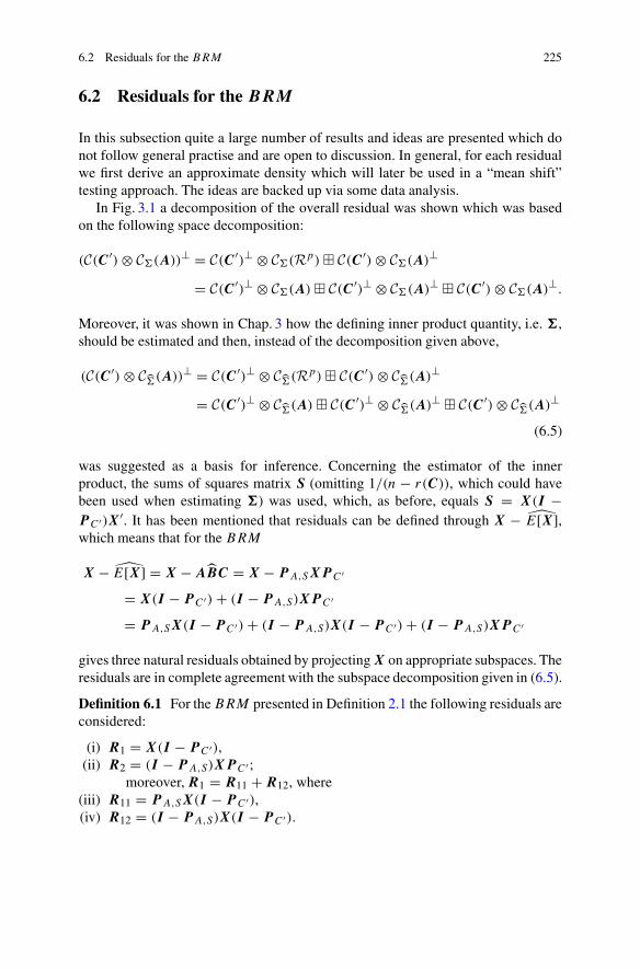
6.2 Residuals for the BRM 225
6.2 Residuals for the BRM
In this subsection quite a large number of results and ideas are presented which donot follow general practise and are open to discussion. In general, for each residualwe first derive an approximate density which will later be used in a “mean shift”testing approach. The ideas are backed up via some data analysis.
In Fig. 3.1 a decomposition of the overall residual was shown which was basedon the following space decomposition:
(C(C′) ⊗ C(A))⊥ = C(C′)⊥ ⊗ C(Rp) � C(C′) ⊗ C(A)⊥
= C(C′)⊥ ⊗ C(A) � C(C′)⊥ ⊗ C(A)⊥ � C(C′) ⊗ C(A)⊥.
Moreover, it was shown in Chap. 3 how the defining inner product quantity, i.e. �,should be estimated and then, instead of the decomposition given above,
(C(C′) ⊗ C(A))⊥ = C(C′)⊥ ⊗ C
(Rp) � C(C′) ⊗ C(A)⊥
= C(C′)⊥ ⊗ C(A) � C(C′)⊥ ⊗ C
(A)⊥ � C(C′) ⊗ C(A)⊥
(6.5)
was suggested as a basis for inference. Concerning the estimator of the innerproduct, the sums of squares matrix S (omitting 1/(n − r(C)), which could havebeen used when estimating �) was used, which, as before, equals S = X(I −P C ′)X′. It has been mentioned that residuals can be defined through X − E[X],which means that for the BRM
X − E[X] = X − ABC = X − PA,SXP C ′
= X(I − P C ′) + (I − PA,S)XP C ′
= P A,SX(I − PC ′) + (I − P A,S)X(I − P C ′) + (I − PA,S)XP C ′
gives three natural residuals obtained by projecting X on appropriate subspaces. Theresiduals are in complete agreement with the subspace decomposition given in (6.5).
Definition 6.1 For the BRM presented in Definition 2.1 the following residuals areconsidered:
(i) R1 = X(I − PC ′),(ii) R2 = (I − P A,S)XPC ′ ;
moreover, R1 = R11 + R12, where(iii) R11 = P A,SX(I − P C ′),(iv) R12 = (I − PA,S)X(I − P C ′).

226 6 Residuals
Fig. 6.2 For the BRM thethree different residuals, R11,R12 and R2, are presented.Moreover, the residualR1 = R11 + R12 can beunderstood
These residuals are illustrated in Fig. 6.2. Note that in Chap. 3, instead of R11, R12and R2, the following notations were used, R11, R12 and R2, because there the aimwas to highlight the fact that the inner product had been estimated.
In principle one would like to find the distribution of the residuals, but, as forthe MLEs of the parameters in the BRM , useful expressions for the distributions(densities) do not exist for R11, R12 and R2. Therefore, density approximations willalso take place for the residuals and these approximations will serve as a basis for anevaluation via a likelihood based test procedure. However, note that, in particular,the residual R1 = R11 + R12 = X(I − PC ′) is normally distributed.
Moreover, although the decomposition of the tensor space seems to be natural,it is even more important that the objects, i.e. the residuals, should be interpretable.Therefore, it is of interest to note that the quantities in Definition 6.1 have a clearmeaning, explained below.
• R1 gathers the differences between the “observations”, X, and the “mean”,XP C ′ . The residual can be used to detect observations which deviate from theothers without taking into account any model assumption.
• R2 gathers the differences between the “mean”, XP C ′ , and the estimated model,ABC = PA,SXP C ′ . The residual gives a hint of the appropriateness of themodel assumptions about the mean structure.
• R11 gathers the differences between the “observations”, X, and the “mean”,XP C ′ , relative to the within-individuals model. The residual is useful fordetecting if observations do not follow the “within-individuals” model.
• R12 is the overall residual and gathers the differences between the “obser-vations”, X, and the “mean”, XP C ′ , relative to the case where the within-individuals model does not hold.
In Fig. 6.3 the four different residuals are presented for the Potthoff and Roy (1964)data set previously considered in Example 1.7. In Fig. 6.3d the model is evaluatedvia R2. One can observe that there is a better fit for the girls than for the boys, and itis clearly indicated that it is worthwhile investigating whether different models canbe used for the girls and for the boys. For example, it can be of interest to apply anEBRM2
B . Moreover, in Fig. 6.3a–c there are interesting observations which will behighlighted in the following presentation. However, the main problem which we are

6.2 Residuals for the BRM 227
(a) (b) (c) (d)
Fig. 6.3 The residuals R1o, R2o, R11o and R12o (see Definition 6.1) for the Potthoff and Roy(1964) data presented in Table 1.2. On the x-axis the 27 observations are listed. The first 11observations concern the girls and the others concern the boys. On the y-axis the values of theresiduals are presented. A linear model over time has been applied and the estimators are given inExample 3.1. Under (a), R1o is presented and then in (b) and (c) the split into R11o and R12o isgiven. The plot in (d) shows R2o, with the four lines per gender corresponding to the four ages andthe four estimated mean values
going to address is to obtain the distribution of the largest residual and, as mentionedabove, this will be dealt with using probabilistic arguments.
Next we prepare for density approximations of the residuals, i.e. we derive themean and dispersion for the different residuals. Additionally, the moments give abasic understanding of the residuals.
Theorem 6.1 Let R1, R2, R11 and R12 be given in Definition 6.1, and
c1 = n − r(C) − p + r(A)
n − r(C), c2 = p − r(A)
n − r(C) − p + r(A) − 1, (6.6)
where it is assumed that n − r(C) − p + r(A) − 1 > 0. Then
(i) E[R1] = 0, E[R2] = 0, E[R11] = 0, E[R12] = 0;(ii) D[R1] = (I − PC ′) ⊗ �;
(iii) C[R1,R2] = 0, C[R2,R12] = 0, C[R2,R11] = 0, C[R11,R12] = 0;(iv) D[R2] = PC ′ ⊗ �P Ao,−1 + c2P C ′ ⊗ P A,�;(v) D[R11] = c1(I − PC ′) ⊗ PA,�;
(vi) D[R12] = (I − P C ′) ⊗ �P Ao,−1 + (1 − c1)(I − PC ′) ⊗ PA,�.
Proof Since Ao′X and X(I − P C ′) both have an expectation equal to 0 and the
residuals are odd functions in X, the expectation of any residual in statement (i)equals 0.

228 6 Residuals
The result in statement (ii) follows because X(I−P C ′) ∼ Np,n(0,�, (I−P C ′)).For statements (iii)–(vi), it is useful to rewrite the residuals in a canonical form.
Let, as in (4.32),
Ao′ = H (Ip−r(A) : 0)��−1/2, (6.7)
where H is a non-singular matrix, �′ = (�′1 : �′
2): p × (p − r(A)) : p × r(A)
is orthogonal and �1/2 is a symmetric square root. Define Y = (Y ′1 : Y ′
2)′ ∼
Np,n(0, I , I − P C ′) with Y 1: (p − r(A)) × n, Y 2: r(A) × n, and let Z ∼Np,n(0, I ,P C ′). Moreover, note that Z = (Z′
1 : Z′2)
′, with Z1: (p − r(A)) × n, isdistributed independently of Y and hence also of Y 1 and Y 2. Using these matrices itfollows that the distribution of the residuals given in Definition 6.1 can be describedas follows:
• R2 = (I −P A,S)XP C ′ is distributed as �1/2�′1Z1 +�1/2�′
2Y 2Y′1(Y 1Y
′1)
−1Z1;• R1 = X(I − P C ′) is distributed as �1/2�′Y , i.e. is normally distributed;• R11 = P A,SX(I − P C ′) is distributed as �1/2�′
2Y 2(I − Y ′1(Y 1Y
′1)
−1Y 1);(6.8)
• R12 = (I − P A,S)X(I − P C ′) is distributed as
�1/2�′1Y 1 + �1/2�′
2Y 2Y′1(Y 1Y
′1)
−1Y 1.
Moreover,
�1/2�′1�1�
1/2 = � − A(A′�−1A)−A′, �1/2�′2�2�
1/2 = A(A′�−1A)−A′.
(6.9)
In statement (iii) it is affirmed that the residuals R11, R12 and R2 are uncorrelated.Because Y 1 and Y 2 are independent,
C[R11,R12] = E[vec{�1/2�′2Y 2(I − P Y ′
1)}vec′{�1/2�′
1Y 1}]+E[vec{�1/2�′
2Y 2(I − P Y ′1)}vec′{�1/2�′
1Y 2P Y ′1}]
= E[(I − Y ′1(Y 1Y
′1)
−1Y 1)Y′1(Y 1Y
′1)
−1Y 1] ⊗ �1/2�′2�2�
1/2 = 0.
Furthermore, because Z1 is independent of Y , C[R2,R12] = 0 and C[R2,R11] =0. Hence, statement (iii) has been established.

6.2 Residuals for the BRM 229
Now it is shown concisely that statements (iv)–(vi) are true. Concerning state-ment (iv), it follows, since Y 2 is independent of Y 1 and Z1, that
D[R2] = PC ′ ⊗(
�1/2�′1�1�
1/2
+�1/2�′2E[Y 2Y
′1(Y 1Y
′1)
−1(Y 1Y′1)
−1Y 1Y′2]�2�
1/2)
and the expectation in this expression is given in Appendix B, Theorem B.21 (vii).Next, when studying D[R12] in statement (vi), since Y 2 is independent of Y 1,
D[R12] = (I − P C ′) ⊗ (�1/2�′1�1�
1/2 + E[P Y ′1] ⊗ �1/2�′
2�2�1/2).
Theorem B.23 (ii) in Appendix B implies
E[P Y ′1] = p − r(A)
n − r(C)(I − PC ′)
and thus statement (vi) is verified. Finally, for statement (v), one can note that R11and R12 are uncorrelated and sum to R1, from which the expression in statement(v) can be obtained. ��In Theorem 6.1 (iii) it was given that the three different residuals are pairwise uncor-related. A natural question arises as to whether the residuals are indeed independent.Unfortunately the answer is negative, i.e. the residuals are not independent. One wayof showing this is to study higher-order mixed moments of the residuals; e.g. onecan show that
E[R11R′11 ⊗ R2R
′2] �= E[R11R
′11] ⊗ E[R2R
′2].
In univariate linear models or the MANOVA model the residuals and the estimatedmean are independent. If this were true for the BRM , this fact could be exploited,but once again a negative answer appears. Concerning the correlation between theresiduals and the mean estimator, the following theorem holds.
Theorem 6.2 Let R2, R11 and R12 be given in Definition 6.1, and ABC =P A,SXP C ′ . Then
(i) C[R11,ABC] = 0;(ii) C[R12,ABC] = 0;
(iii) C[R2,ABC] = − p−r(A)n−r(C)−p+r(A)−1P C ′ ⊗P A,�, if n−r(C)−p+r(A)−
1 > 0.
Proof Since XP C ′ is independent of R11 and R12 both statements (i) and (ii) followimmediately. Concerning statement (iii),
C[R2,ABC] = C[XPC ′,ABC] − D[ABC] = P C ′ ⊗ P a,� − D[ABC],
and D[ABC] was presented in Theorem 4.3 (ii). Hence, statement (iii) is verified.��

230 6 Residuals
Since R2 measures the deviation from the model, but according to statement (iii)of the theorem is also correlated with ABC, any conclusion based on R2 shouldalso take this fact into account; i.e. marginal inference based on R2 should not beperformed uncritically. Moreover, note that the covariance is negative and that it“diminishes” when n increases.
The next theorem includes unbiased estimators of the dispersion of the residualswhich can be used when quickly evaluating them, i.e. to decide about the tails of thedistribution of the residuals. However, it is questionable to suppose unbiasednessfor functions of quadratic expressions, since in general quadratic forms are notsymmetrically distributed. On the other hand, there are no obvious alternativeestimators which are easily calculated.
Theorem 6.3 Let D[R2], D[R11] and D[R12] be given in Theorem 6.1 and �
in Theorem 3.1. Then, the following estimators are unbiased estimators of thedispersion of the residuals (the constants c1 and c2 are presented in Theorem 6.1):
(i) if n − r(C) − p + r(A) > 0,
D[R11] = nn−r(C)
(I − P C ′) ⊗ P A,�;
(ii) if n − r(C) − p + r(A) − 1 > 0,
D[R12] = (I − PC ′) ⊗ (� + ( r(C)n
(1 − c2) − c1)n
n−r(C)−p+r(A)P A,
�);
(iii) if n − r(C) − p + r(A) − 1 > 0,
D[R2] = PC ′ ⊗ (� + (c2 − 1 + r(C)n
(1 − c2))n
n−r(C)−p+r(A)P A,
�).
Proof The proof of the three statements is based on a combination of E[�], givenin Theorem 4.6 (ii), and (see Theorem B.20 (v) in Appendix B)
nA(A′�
−1A)−A′ = A(A′S−1A)−A′
∼ Wp(A(A′�−1A)−A′, n − r(C) − p + r(A)).
��The condition n−r(C)−p+r(A) > 0 in statement (i) and n−r(C)−p+r(A)−1 >
0 in statements (ii) and (iii) are needed to secure existence of c1 and c2.

6.3 Distribution Approximations of the Residuals in the BRM 231
6.3 Distribution Approximations of the Residuals in theBRM
In the previous section the most basic properties for the three residuals R11, R12and R2 were presented. Next the distribution of the residuals is studied, but thiscan only be performed approximately. As for the MLEs, an Edgeworth-type densityapproximation will be derived.
Since n−1S converges to � in probability, as n → ∞ (see Appendix B,Theorem B.18 (ii)), the residuals R11, R12 and R2 can respectively be approximatedas follows by
R11N = P A,X(I − PC ′) ∼ Np,n(0,A(A′�−1A)−A′, I − P C ′), (6.10)
R12N = (I − P A,)X(I − P C ′) ∼ Np,n(0,�Ao(Ao′�Ao)−Ao′�, I − P C ′),(6.11)
and
R2N = (I − PA,)XP C ′ ∼ Np,n(0,�Ao(Ao ′�Ao)−Ao′�,P C ′), (6.12)
respectively. Moreover, R11 = R11N −U11, R12 = R12N −U 12, R2 = R2N −U2,where
U11 = (PA, − P A,S)X(I − P C ′), U 12 = −U 11 (6.13)
and
U 2 = (PA, − P A,S)XPC ′ . (6.14)
In Sect. 5.3 the density approximation of the mean estimator in the BRM
was considered and a U -matrix (“error matrix”) was obtained, which in turn wasindependent of the normally distributed approximating quantity. This is not true forthe above-suggested U11, U 12 and U2. These quantities only satisfy C[R•N,U•] =0, i.e. the U -matrices are uncorrelated with the quantities which approximatethe residuals. Under some mild conditions, according to Corollary 5.3, we canapproximate the density of the residual with another density, although this time noerror bound for the approximation can be presented. Concerning U 11 and U 12, themain difference compared with the mean estimator in the BRM is that X(I − P C ′)is not independent of S, unlike XP C ′ which is part of the mean. The independencebetween S and XPC ′ was important when considering the mean estimator. To findan error bound of the approximation is, of course, of interest. However, this ismore crucial for the density approximation of the mean estimators than that of theresiduals. One reason is that in this case one intends to compare the residuals fromall the different subjects and, since one is carrying out the same procedure for each

232 6 Residuals
subject, it is often not very essential to find an upper error bound, because it will notincrease the discrimination power among the subjects. The matter of importanceis the distribution of the multiple comparison procedure which is applied for eachresidual, which will be treated in detail in Sect. 6.4.
Now some basic moment relations are presented which will be used in thetheorems presented below where Edgeworth-type approximations are presented.The results follow from Theorem 6.1, where c2 (used below) is also defined andsupposed to exist. From (6.10) to (6.12) the said moment relations are as follows:
E[R11] = E[R11N ] = 0, E[R12] = E[R12N ] = 0, E[R2] = E[R2N ] = 0,
(6.15)
D[R11] − D[R11N ] = −p − r(A)
n − r(C)(I − P C ′) ⊗ PA,�, (6.16)
D[R12] − D[R12N ] = p − r(A)
n − r(C)(I − PC ′) ⊗ P A,�, (6.17)
D[R2] − D[R2N ] = c2P C ′ ⊗ P A,�. (6.18)
Note that (6.16) shows that the approximation suggested by (6.10) has a largervariation than the quantity which is to be approximated and this is not desirable.The result in (6.16) indicates that something is not optimal, which follows from thefact that S and X(I − P C ′) are dependent.
However, the approximation can be sharpened, somewhat, and an approximationwill indeed be derived whose error has a mean which equals 0 and is independent ofthe approximating variable. The idea is to manipulate R11N in R11 = R11N − U 11.Instead of R11N ,
P A,XM(I − P C ′) = P A,XM
(
0 00 In−p+r(A)
)
(I − P C ′)
+ PA,XM
(
Ip−r(A) 00 0
)
(I − P C ′)
will be used, where M is an orthogonal matrix which satisfies
P ′Ao,S−1X(I − PC ′) = XM
(
Ip−r(A) 00 0
)
M ′;

6.3 Distribution Approximations of the Residuals in the BRM 233
i.e. an eigenvalue decomposition of the idempotent matrix (I−P C ′)X′Ao(Ao′X(I−
P C ′)(I − P C ′)X′Ao)−Ao′X(I − P C ′) has taken place. Thus,
R11 = P A,XM
(
0 00 I n−p+r(A)
)
(I − P C ′)
+ P A,XM
(
Ip−r(A) 00 0
)
(I − P C ′) − U 11.
The explanation for our next result is that P A,X and PA,XM have marginallythe same normal distribution, since M ′M = I and M is independent of PA,X,but PA,XM has some advantages in comparison with P A,X, i.e. it is possibleto have an approximating quantity which is independent of the error.
Theorem 6.4 The distribution of the residual R11 given in Definition 6.1 can beapproximated through the difference
R11 = ˜R11N − U11x,
where
˜R11N = PA,XM
(
0 00 In−p+r(A)
)
(I − P C ′)
is normally distributed and
U 11x = −P A,XM
(
Ip−r(A) 00 0
)
(I − PC ′) + (P A, − P A,S)X(I − PC ′),
with ˜R11N and U 11x being independently distributed and M satisfying
M
(
Ip−r(A) 00 0
)
M ′
= (I − P C ′)X′Ao(Ao′X(I − PC ′)(I − P C ′)X′Ao)−Ao′
X(I − P C ′).
Proof First note that
(P A, − PA,S)X(I − P C ′) = P A,(I − P A,S)X(I − P C ′)
= P A,P ′Ao,S−1X(I − P C ′) = P A,XM
(
Ip−r(A) 00 0
)
M ′.

234 6 Residuals
It will be proved that ˜R11N and U11x are independently distributed. Note thatA′�−1X and Ao′
X are independent, which implies that PA,XM and M areindependent, since M is a function of Ao′
X and the distribution of XM is
independent of M . Moreover, P A,XM
(
0 00 I n−p+r(A)
)
is independent of
P A,XM
(
Ip−r(A) 00 0
)
, since the expressions comprise different independent
observations. Thus, the theorem has been established. ��Note that the sizes of I • in the decomposition, i.e. Ip−r(A) and In−p+r(A), followfrom
r((I − P C ′)X′Ao) = r(SAo) = r(Ao) = p − r(A).
Hence, the distribution of R11 is approximated with a subset of XM . It is somewhatunsatisfactory that the decomposition is not unique and there are in fact
(
np−r(A)
)
possibilities to approximate.For the Edgeworth-type approximations of the density for R11 in the following,
moments of order 1 and 2 are needed and for their error terms moments of the fourthorder have to be obtained. Therefore, it is noted that
E[R11] = E[˜R11N ] = 0,
D[R11] − D[˜R11N ]
= (c1(I − P C ′) − (I − P C ′)
(
0 00 In−p+r(A)
)
(I − PC ′)) ⊗ PA,�, (6.19)
with c1 defined in Theorem 6.1. Unfortunately, the difference in (6.19) is not positivedefinite. The derivation of the fourth-order moments will be omitted, since this needsrelatively lengthy calculations, but these calculations follow those performed whenobtaining higher-order moments for the estimators in the BRM . Moreover, since thedensities for R11 and ˜R11N do not exist, linear combinations of the residuals withdispersion matrices which are of full rank will be considered. Indeed, residuals arecommonly evaluated via KR•L, where K and L may be vectors and, in particular,unit basis vectors which select one element of R• (• means that it can be R11, R12,R1 or R2). The proof of the next theorem follows from Theorem 5.2 and (6.19).
Theorem 6.5 For the BRM , let the residual R11 be as given in Definition 6.1, letK: p1 × p and L: n × n1, both of which are known, and let
K˜R11NL ∼ Np1,n1(0,KA(A′�−1A)−A′K ′,D),
D = L′(I − P C ′)
(
0 00 In−p+r(A)
)
(I − P C ′)L.

6.3 Distribution Approximations of the Residuals in the BRM 235
Then an Edgeworth-type expansion of the density of KR11L, via the density ofK˜R11NL and under the assumption that D[K˜R11NL] is p.d., equals
fKR11EL(KRoL) + r ,
where
fKR11EL(KRoL) = {
1 − 12c1p1tr{L′(I − P C ′)LD−1} + 1
2p1n1
+ 12 tr{(KA(A′�−1A)−A′K ′)−1KRoLD−1
×(c1L′(I − P C ′)L − D)D−1L′R′
oK′}}
×fK˜R11NL(KRoL);
c1 is supposed to exist and is defined in Theorem 6.1, and the leading term of |r | isproportional to E[vec(K(R11 −˜R11N)L)⊗4] which is a function of A, C, K and L.
The two most basic moment properties of KR11EL are now given. Statement (ii) inparticular will be used later.
Corollary 6.1 Let KR11EL be defined via fKR11EL(KRoL), presented in Theo-rem 6.5, where it is assumed that fKR11EL(KRoL) ≥ 0. Then
(i) E[KR11EL] = 0;(ii) D[KR11EL] = c1L
′(I − P C ′)L ⊗ KA(A′�−1A)−A′K ′.
Proof The derivation of statement (ii) follows from Appendix B, Theorem B.23 (i),because according to the theorem
D[KR11EL] = (
1 − 12c1p1tr{L′(I − P C′)LD−1} + 1
2p1n1)
D ⊗ KA(A′�−1A)−A′K ′
+ 12p1tr{D−1(c1L
′(I − P C′)L − D)}D ⊗ KA(A′�−1A)−A′K ′
+(c1L′(I − P C′)L − D) ⊗ KA(A′�−1A)−A′K ′
which is identical to statement (ii). ��Now we switch from a discussion of R11 to a discussion of the other two
residuals, R12 and R2, presented in Definition 6.1. However, for these residualsno results will be presented which correspond to Theorem 6.4, i.e. no modificationlike the one which led to ˜R11N will take place. The next two theorems are based onCorollary 5.3, and density approximations for R12 and R2 are presented.
Theorem 6.6 The distribution of the residual R12 given in Definition 6.1, can beapproximated through the difference
R12 = R12N − U 12,

236 6 Residuals
where R12N and U12 are defined by (6.11) and (6.13), respectively. Let K: p1 × p
and L: n × n1, both of which are known, and
KR12NL ∼ Np1,n1(0,K�P Ao,−1K′,L′(I − P C ′)L).
Then an Edgeworth-type expansion fKR12EL(KRoL) of the density of KR12L, viathe density of KR12NL, under the assumption that D[KR12NL] is p.d., is given by
fKR12EL(KRoL) = {
1 − 12
p−r(A)n−r(C)
n1tr{KPA,�K ′(K�P Ao,−1K ′)−1}+ 1
2c1tr{(K�P Ao,−1K ′)−1KP A,�K ′(K�P Ao,−1K ′)−1
× KRoL(L′(I − P C ′)L)−1L′R′oK
′}}fKR12NL(KRoL),
where c1, supposed to exist, is defined in Theorem 6.1.
Corollary 6.2 Let KR12EL be defined via fKR12EL(KRoL), given in Theo-rem 6.6, where it is assumed that fKR12EL(KRoL) ≥ 0. Then
(i) E[KR12EL] = 0;(ii) D[KR12EL] = L′(I − P C ′)L ⊗ (f1K�P Ao,−1K ′ + c1KP A,�K ′),
where
f1 = 1 − 12
p−r(A)n−r(C)
n1tr{KP A,�K ′(K�P Ao,−1K′)−1}
+ 12c1n1tr{(K�P Ao,−1K ′)−1KP A,�K ′}.
Theorem 6.7 The distribution of the residual R2, given in Definition 6.1, can beapproximated through the difference
R2 = R2N − U 2,
where R2N and U 2 are defined by (6.12) and (6.14), respectively. Let K: p1 × p
and L: n × n1, both of which are known, and
KR2NL ∼ Np1,n1(0,K�P Ao,−1K ′,L′P C ′L).
Then an Edgeworth-type expansion fKR2EL(KRoL) of the density of KR2L, viathe density of KR2NL, under the assumption that D[KR2NL] is p.d., is given by
fKR2EL(KRoL) = {
1 − 12c2p1n1
+tr{(KPA,�K ′)−1KRoL(L′P C ′L)−1L′R′oK
′}}fKR2N L(KRoL),
where c2, supposed to exist, is defined in Theorem 6.1.

6.4 Mean Shift Evaluations of the Residuals in the BRM 237
Corollary 6.3 Let KR2EL be defined via fKR2EL(KRoL), given in Theorem 6.7,where it is assumed that fKR2EL(KRoL) ≥ 0, and suppose that c2p1n1 ≤ 2.Then
(i) E[KR2EL] = 0;(ii) D[KR2EL] = (
1− 12c2p1n1+n1tr{(KP A,�K ′)−1K�P Ao,−1K ′})L′P C ′L
⊗K�PAo,−1K ′
+2L′PC ′L⊗K�PAo,−1K ′(KP A,�K ′)−1K�P Ao,−1K ′.
6.4 Mean Shift Evaluations of the Residuals in the BRM
In the presentation of Sect. 6.3, approximate densities of the residual matrices R11,R12 and R2 have been obtained. The expressions depend on unknown dispersionparameters and if one uses the densities directly, the parameters have to be replacedby estimates. This can be carried out and then it is possible to look for extremevalues in the data set i.e., one tries to understand if the extreme observations are inthe tail of the distribution.
However, one should remember that a weak point of Edgeworth-type expansionsis that the tails of the distributions may be poorly estimated.
Another approach, already demonstrated in Sect. 6.1, where it was shown how itcan work for the MANOVA model, is based on statistical testing for extreme obser-vations. This can be achieved by studying the so-called mean shift assumptions. Inthis case a model is assumed for the residuals. Let R• represent any of the residualsR11, R12, R1 and R2. Then the model which will be studied can, in principle, bewritten as follows:
R• = F�G + E•, (6.20)
where the density for E• is one of the densities presented in Theorem 6.5,Theorems 6.6 and 6.7 or the matrix normal density.
The F and G matrices in (6.20) can correspond to the five cases mentioned inSect. 6.1, i.e. F = 1, F = dj or F = I , and G = 1′, G = e′
i or G = I , where dj
and ei stand as usual for the unit basis vectors.A test can be constructed for testing H0 : � = 0 via the previous theorems
where density approximations were derived. The idea is to construct, for any given�, a test which is similar to the likelihood ratio test. Many tests will be performed,e.g. for each i and j in {d i , ej }, and the maximum value or some of the largest valuesof the test statistics are of interest. Even if we were to estimate �, the distributionof the test statistic would still be a function of �. Therefore, no energy will bespent on obtaining special estimators of � so that pivot quantities will appear whichare completely independent of all the parameters. Instead, when interpreting thedistribution of the mean shift test, only the MLE of � from the BRM will be utilized

238 6 Residuals
as a consistent plug-in estimator. An obvious alternative estimator which might beused is the unbiased estimator presented in Theorem 4.7.
In the following a number of test statistics will be presented which will later beevaluated through a parametric bootstrap approach. Let us start with R12 and somepreparations. The density approximation given by Theorem 6.6 cannot be directlyapplied if D[KR12EL] is singular, and therefore an appropriate working densityhas to be found. For example, when applying a likelihood-based approach, densitieshave to exist. Under H0, i.e. with no mean shift, the information about the residualsis solely available on the space connected to the eigenvalues of D[R12N ] which arelarger than 0, where the dispersion is given in Theorem 6.6. Therefore, D[R12N ] isspectrally decomposed as
D[R12N ] = V V ′ ⊗ WW ′, V : n × (n − r(C)), W : p × (p − r(A));
i.e. �P Ao,−1 = WW ′ and I − P C ′ = V V ′. Note that W is a functionof �, and later, when analysing data, W is obtained by factorizing �P Ao,−1 ,i.e. �P Ao,−1 = WW ′. A modified non-singular residual can be obtained by pre-and post-multiplying R12 in the following suitable way:
RN12 = (W ′W )−1W ′R12V (V ′V )−1;
this density approximation leads to a non-singular distribution. By choosing K =(W ′W )−1W ′ and L = V (V ′V )−1 Theorem 6.6 can be applied directly and anappropriate density has been obtained. Hence, the following formal model will be“tested”:
RN12;ij = Kdj θe′
iL + E12, (6.21)
where E12 has the density presented in Theorem 6.6 with the particular choices ofK and L provided above. Moreover, note that RN
12;ij is the same matrix as RN12 but
in order to indicate which residual is to be tested, RN12;ij is used. It follows that
D[KRN12L] = Ip1n1 , where p1 = p − r(A), n1 = n − r(C) and it is supposed that
K is a function of �, not �. Note that RN12 bears the same amount of information
as R12.Let LN
12;ij (θ) and LN12;ij denote the likelihood for RN
12;ij under H1: θ �= 0 and H0:θ = 0, respectively, where under H1 an estimator of θ is needed. If a strict likelihoodratio test were to be constructed, θ would have to be the MLE for θ . However, thisestimator can only be obtained via an iterative algorithm due to the expression forthe density of E12 given in Theorem 6.6. Instead a least squares approach can beused, e.g.
minθ
tr{T −1(RN12;ijo − Kdj θe′
iL)()′},

6.4 Mean Shift Evaluations of the Residuals in the BRM 239
where
T = f1I + c1KP A,�K ′; (6.22)
f1 and c1 are presented in Corollary 6.2 and Theorem 6.1, respectively, and RN12;ijo
is the observation of RN12;ij which equals
RN12;ijo = (W ′W )−1W ′R12oV (V ′V )−1.
A unique least squares solution under the assumption of a known � is given by
θo = (d ′jK
′T −1Kdj )−1d ′
jK′T −1RN
12;ijoL′ei (e
′iLL′ei )
−1. (6.23)
If one replaces � by its MLE presented in Theorem 3.1, there is enough informationfor forming a test statistic for testing H0: θ = 0, which is then given by
Tijo = LN12;ij (θo)
LN12;ij
. (6.24)
However, one may question this approach, because it depends on the approximat-ing density and its singularity; i.e. one may question whether an estimator shouldbe based on the matrices K and L, which appear because of the choice of theapproximating distribution.
An alternative approach is to use the observation (R12o)ij as an estimate of θ
when considering dj θe′i . This implies that the likelihood ratio in (6.24) is in fact a
ratio between a density without the ij th observation (with an improper standardizingconstant) and a density for all the observations. In the following examples this latterchoice of θo will be applied.
Let ij1 denote the pair of indices which corresponds to maxij Tijo, ij2 is the pairof indices which corresponds to the second largest value in {Tijo} and ij3 is the pairof indices which identifies the third largest value in {Tijo}. Now the remaining taskis to determine the distribution of the corresponding Tij1 , Tij2 and Tij3 .
The statistic in (6.24) has been constructed via density approximations and a“semi-likelihood ratio test” approach. If the observations are replaced by theircorresponding random variables, we can write as follows:
Tij = LN12;ij (θ)
LN12;ij
, θ = d ′jR12ei , (6.25)
and our interest is, for example, Tij1 and its distribution. One way of handling thisdistribution is via simulations. However, it is less clear how these simulations shouldbe performed. The density presented in Theorem 6.6 can be used and via a random

240 6 Residuals
number generating algorithm, suited to handling a known multivariate density, onecan obtain observations so that the distribution for Tij1 can be described.
In this book a somewhat easier approach is applied. The proposed strategy is togenerate observations, Xo, according to
X ∼ Np,n(0,�o, I ),
where � is presented in Theorem 3.1. In other words the parametric bootstrapphilosophy is applied. Note that other relevant estimators of � could also have beenused. The observations Xo are then used to calculate R12o = (I − P A,o
)Xo(I −P C ′). Thereafter LN
12;ij (θo) and LN12;ij are calculated, as well as {Tijo}. Thus, Tijk ,
k = 1, 2, 3, is obtained. This process can be repeated a large number of times, anda density can thereby be estimated, which can be used to determine how far out inthe tails of the distributions the original deviating residuals appear.
When working with vector-valued residuals, instead of single elements of theresidual matrix, as above, there is one immediate advantage of using a test statisticinstead of directly working with the density. The advantage is that it is easier to drawconclusions from a one-dimensional test statistic than to draw conclusions based onan evaluation of a multivariate density function.
In the next example the above ideas are illustrated.
Example 6.1 (The Classical Potthoff and Roy (1964) Data Set) The data havealready been used for illustration, see Examples 1.7 and 3.1. The residual R12o =(I − P
A,S−1o
)Xo(I − P C ′) is presented in Table 6.1 together with the test statisticpresented in (6.25).
It is seen from Table 6.1 that the test statistic reflects the size of the componentsin R12o, which supports the presented approach. Hence, the remaining task is tofind the distribution of the large residuals, taking into account the fact that onehas to investigate 108 correlated observations from 27 independently distributedindividuals. In Table 6.2, simulated quantiles for Tij1 , Tij2 and Tij3 are presented.It is only T203o = 1367.0 which is significant, since it is larger than Tij1o at a95% level. Moreover, note the small value T201o = 0.5. Since maximum likelihoodestimators are not used, the test statistic can become smaller than 1, but this value isclearly much smaller than the other values. Since both the smallest and the largestvalue appeared for the same individual, i.e. #20, and we know beforehand thatobservations within individuals are correlated, we can only conclude that individual#20 deviates from the others. Table 6.2 also gives simulated quantiles for theresiduals corresponding to the three largest (by absolute value) residuals, R12;ij1o,R12;ij2o and R12;ij3o. The results are in agreement with those based on the teststatistic given by (6.25); i.e. individual #20 deviates. It is interesting to determinehow large the residuals need to be in order to become significant; i.e. even if theresiduals are asymptotically normally distributed with mean 0 and a variance which,according to Table 6.1, does not seem to imply great variability, large values are stillnot very unlikely to appear. ��

6.4 Mean Shift Evaluations of the Residuals in the BRM 241
Table 6.1 The residuals R12o = (I − PA,S−1
o)Xo(I − P C′ ) = (R12;ijo) and the test statistic
given in (6.25) applied to the Potthoff and Roy (1964) data presented in Table 1.2
Residuals Test statistics
id Gender R12;i1o R12;i2o R12;i3o R12;i4o Ti1o Ti2o Ti3o Ti4o
1 F 1.22 −0.87 −0.29 0.16 2.0 1.5 1.1 1.0
2 F 0.77 −0.54 0.33 0.07 1.2 1.1 1.0 1.0
3 F −1.12 0.80 −0.10 −0.13 1.7 1.4 1.0 1.0
4 F 0.05 −0.04 −0.44 0.03 1.0 1.0 1.1 1.0
5 F −0.54 0.38 −0.51 0.04 1.1 1.1 1.0 1.0
6 F −0.08 0.05 −0.64 0.03 1.0 1.0 1.1 1.0
7 F 0.16 −0.12 −0.71 0.06 1.0 1.0 1.2 1.0
8 F 0.29 −0.21 −0.02 0.03 1.0 1.0 1.0 1.0
9 F −0.28 0.21 0.88 −0.08 1.1 1.0 1.3 1.0
10 F −1.00 0.71 0.11 −0.12 1.6 1.3 1.0 1.0
11 F 0.55 −0.38 1.37 −0.01 1.0 1.0 1.3 1.0
12 M 1.47 −1.04 0.47 0.15 2.2 1.6 0.9 1.0
13 M 0.02 −0.03 −1.55 0.09 1.0 1.0 1.8 1.0
14 M 0.97 −0.70 −1.34 0.19 1.8 1.4 2.2 1.0
15 M −1.49 1.05 −0.38 −0.15 2.3 1.7 0.9 1.0
16 M −1.51 1.06 −1.84 −0.08 1.6 1.4 1.1 1.0
17 M −0.18 0.13 −0.02 −0.02 1.0 1.0 1.0 1.0
18 M 0.64 −0.45 −0.02 0.02 1.2 1.1 1.0 1.0
19 M 1.71 −1.21 0.41 0.18 3.0 2.0 0.9 1.0
20 M 2.18 −1.49 6.87 −0.12 0.5 0.9 1367.0 1.0
21 M 0.19 −0.13 1.09 −0.04 1.0 1.0 1.3 1.0
22 M 0.04 −0.03 −0.58 0.04 1.0 1.0 1.1 1.0
23 M −0.33 0.22 −1.69 0.05 0.9 1.0 1.7 1.0
24 M −2.78 1.97 −0.25 −0.31 22.2 6.9 0.8 1.1
25 M −1.71 1.22 0.18 −0.21 3.6 2.2 1.1 1.0
26 M 0.14 −0.11 −1.34 0.09 1.0 1.0 1.6 1.0
27 M 0.64 −0.45 −0.02 0.08 1.2 1.1 1.0 1.0
Up to now only single observations, i.e. d ′jR12ei , have been studied. If instead
individuals are of interest, R12ei will be exploited and there are two different modelswhich one should, “naturally”, investigate. The first model equals
RN12;i = Kθe′
iL + E12, (6.26)
where K, L and E12 are as in (6.21) and RN12;i = RN
12, where i is only usedto indicate the mean shift for the ith observation; the notation also applies to thelikelihood functions LN
12;i(θo) and LN12;i given below. Now θ is a vector of size p,
meaning that there is a shift for each component of the residual connected to the ithobservation vector. If, however, the mean shift is the same for each component, then

242 6 Residuals
Table 6.2 Estimated quantiles for Tij1 , Tij2 and Tij3 connected to the test statistics Tij1o, Tij2o
and Tij3o, with Tij defined in (6.25), and applied to the Potthoff and Roy data set presented inTable 1.2
Quantile Tij1o Tij2o Tij3o R12;ij1o R12;ij2o R12;ij3o
100% max 1.7×10⁶ 1.3×10⁴ 1.9×10³ 8.6 7.5 6.0
99% 3.9×10³ 2.2×10² 66.3 6.4 5.2 4.6
95% 4.2×10² 64.2 27.4 5.5 4.5 4.0
90% 1.7×10² 37.7 18.1 5.0 4.2 3.7
75% 51.3 17.5 10.2 4.3 3.7 3.3
50% 18.5 9.1 6.3 3.7 3.1 2.8
25% 8.9 5.5 4.2 3.1 2.7 2.5
10% 5.3 3.8 3.1 2.7 2.4 2.2
5% 4.1 3.1 2.6 2.5 2.2 2.0
1% 2.7 2.3 2.1 2.1 1.9 1.8
0% min 1.6 1.5 1.5 1.6 1.5 1.5
Estimated quantiles are given for the three largest (by absolute value) residuals, R12;ij ko,k = 1, 2, 3, obtained from the same data set. The estimated quantiles are based on 10,000simulations
instead of (6.26) the following second model can be used:
RN12;i = K1pθe′
iL + E12, (6.27)
where E12 follows the distribution (density) presented in Theorem 6.6.Let us start by constructing a test for H0: θ = 0 in (6.26). Via a least squares
approach, an estimate of θ is given by
θo = (K ′T −1K)−1K ′T −1RN12;ioL
′ei (e′iLL′ei )
−1,
where T is given in (6.22), and in T as well as RN12;i the unknown � is replaced
by an appropriate estimate. Alternatively, similar to the treatment of R12;ij , anunweighted estimator,
θ = R12ei , (6.28)
can be utilized. In this case, a test statistic corresponding to (6.24), when, forexample, (6.28) is used, equals
Tio = LN12;i(θo)
LN12;i
, (6.29)
where LN12;i equals LN
12;ij , given above, i.e. the likelihood under the H0 of no mean
shift. Moreover, LN12;i(θo) is the likelihood under the alternative hypothesis where θ

6.4 Mean Shift Evaluations of the Residuals in the BRM 243
Table 6.3 The same data as in Table 6.1 are analysed, but in this table the test statistic for column-wise mean shift, Tio, based on (6.28) and (6.29), is presented
Individual
1 2 3 4 5 6 7 8 9 10 11 12 13 14
Tio 2.4 1.3 1.8 1.1 1.1 1.1 1.2 1.0 1.4 1.7 1.5 2.5 1.8 3.5
T io 1.0 1.0 1.0 1.0 1.1 1.1 1.1 1.0 1.2 1.0 1.5 1.0 1.6 1.5
Individual
15 16 17 18 19 20 21 22 23 24 25 26 27
Tio 2.6 3.2 1.0 1.2 3.5 9379.2 1.3 1.1 1.8 36.0 4.6 1.7 1.2
T io 1.0 2.0 1.0 1.0 1.0 9486.7 1.3 1.1 1.8 1.0 1.0 1.4 1.0
The test statistic for column-wise mean shift, T io, based on (6.30) and (6.31), is also shown
has been estimated by the ith column of R12o, and hence the likelihood LN12;i (θo),
besides including a correct standardization constant, is the likelihood of all theobservations except the ith one. Based on Tio in (6.29), the distribution of the teststatistic Tik , k = 1, 2, 3, can be simulated, i.e. the distribution of the largest, secondlargest and third largest value of the statistic can be simulated. The procedure isillustrated in the next example.
Example 6.2 (The Classical Potthoff and Roy (1964) Data Set, Given in Table 1.2.)The residual R12o = (I − P A,S−1)Xo(I − P C ′) was presented in Table 6.1, and inTable 6.3 the test statistic of no mean shift in columns according to (6.29) is shownfor the case where (6.28) is used as an estimate of θ . Moreover, the quantiles of thethree largest values of the test statistic are presented in Table 6.4.
From Tables 6.3 and 6.4 it follows that only individual #20 has an extremeresidual, since T20o = 9379.2 is larger than Ti1o at a 95% level, which is in completeagreement with the results of the mean shift analysis presented in Tables 6.1 and 6.2.Furthermore, in Tables 6.1 and 6.3, one can observe that the behaviour of individual#24 is peculiar too, but it is not significantly peculiar. ��
Now the alternative test procedure based on H0: θ = 0 in (6.27) is discussedin some detail. It is assumed that there is a mean shift which is equal for all thecomponents in a column of R12, for example the ith column. The least squaresapproach yields an estimate of θ which equals
θo = (1′K ′T −1K1)−11′K ′T −1RN12ioL
′ei (e′iLL′ei )
−1, (6.30)
where T is given in (6.22) with � in T replaced by an estimator, for example theunbiased one presented in Theorem 4.7. The replacement of � by � also appliesto RN
12io. Moreover, the hypothesis concerning H0, together with the least squaresapproach, implies a somewhat different interpretation of the residual evaluation thanthat given above, i.e. the interpretation of the test statistic in (6.29). A test statistic

244 6 Residuals
Table 6.4 Estimated quantiles connected to the test statistics Tiko and T iko, k = 1, 2, 3,respectively, defined in (6.29) and (6.31), are presented
Quantile Ti1o Ti2o Ti3o T i1o T i2o T i3o
100% max 7.6×10⁶ 4.1×10⁴ 2.5×10³ 3.0×10⁶ 4.0×10⁴ 1.9×10³
99% 1.7×10⁴ 6.3×10² 1.7×10² 4.4×10³ 2.3×10² 59.5
95% 1.6×10³ 1.6×10² 59.9 4.2×10² 57.0 22.5
90% 5.6×10² 91.4 37.7 1.5×10² 29.5 13.8
75% 1.5×10² 37.2 19.3 37.8 12.2 7.1
50% 44.8 17.3 10.5 11.0 5.5 3.8
25% 18.3 9.1 6.2 4.6 2.9 2.3
10% 9.6 5.7 4.2 2.5 2.0 1.7
5% 7.0 4.4 3.4 2.0 1.6 1.5
1% 4.0 3.1 2.5 1.3 1.2 1.2
0% min 1.7 1.6 1.6 1.0 1.0 1.0
The estimated quantiles are based on 10,000 simulations
corresponding to (6.29) equals
T io = LN12;i(θo)
LN12;i
, (6.31)
where θo is presented in (6.30). Indeed a test based on (6.31) is close to a traditionallikelihood ratio test based on a normally distributed sample with known dispersion,although instead of the normal density, the density in Theorem 6.6 is used. Thetest statistic is illustrated in the next example. However, any significant results onlyreflect that the equal mean shift hypothesis is not true and do not automaticallyimply that the residuals are extreme.
Example 6.3 (The Classical Potthoff and Roy (1964) Data Set Given in Table 1.2)The residual R12o = (I − P
A,S−1o
)Xo(I − P C ′) was presented in Table 6.1, andin Table 6.3 the test statistic for no equal mean shift in columns according to (6.31)is shown. Moreover, in Table 6.4 the distribution for the three largest values of thetest statistic is presented. Once again it follows that individual #20 deviates from theothers. ��Finally, concerning the residual R12, the mean shift tests within the rows of R12 arepresented. A test statistic corresponding to (6.29) for testing H0 : θ = 0 in
R12;j = KdjθL + E12,

6.4 Mean Shift Evaluations of the Residuals in the BRM 245
where θ is a row vector of proper size and the density for E12 is presented inTheorem 6.6, equals
Tjo = LN12;j (θo)
LN12;j
, (6.32)
where θo = d ′jR12o. The notation follows the same ideas as those used when
constructing (6.25) or (6.29). Concerning (6.32), the reader should be warned thatthere are too many parameters involved and the test statistic is rather heuristic.Moreover, a test statistic corresponding to (6.31) for testing H0 : θ = 0 in
RN12;j = Kdj θ1′L + E12
equals
T jo = LN12;j (θo)
LN12;j
, (6.33)
where (with an estimated �)
θo = (d ′jK
′T −1Kdj )−1d ′
jK′T −1RN
12;joL′1(1′LL′1)−1,
and T is given in (6.22). Example 6.4 presents some explicit data analysis.
Example 6.4 (The Classical Potthoff and Roy (1964) Data Set Given in Table 1.2)The residual R12o = (I − P
A,S−1o
)Xo(I − P C ′) was presented in Table 6.1, and inTable 6.5 the test statistic for no mean shift in rows according to (6.32) or (6.33) isshown. Simulations did not reveal any significant values. Because the tests are acrossindividuals, a significant difference in this example would have been somewhatdifficult to explain. ��
Above, R12 has been exploited and next R11 will come into focus. However,all the expressions concerning testing for mean shifts in R11 are similar to thecorresponding expressions for R12. Therefore, a theorem will be presented whichcovers both residuals, but first a number of preparatory notations will be introduced.As before, the problem of singularity of the distribution has to be taken care of
Table 6.5 The data in Table 6.1 are analysed and the test statistics for row-wise mean shift, Tjo
and T jo, given in (6.32) and (6.33), respectively, are presented
Time
8 12 14 16
Tjo 1.4×10⁴ 6.1×10² 6.8×10³ 1.3
T jo 0.7 2.0 0.8 0.7

246 6 Residuals
via bilinear transformations. Let ˜R11N and R12 be defined in Theorem 6.4 andDefinition 6.1, respectively. From the above discussion concerning R12, it followsthat one can use
K12 = (W ′2W 2)
−1W ′2, L12 = V 2(V
′2V 2)
−1, (6.34)
where it is assumed that D[R12N ] = V 2V′2 ⊗ W 2W
′2 and
K11 = (W ′1W 1)
−1W ′1, L11 = V 1(V
′1V 1)
−1, (6.35)
since
D[˜R11N ] = V 1V′1 ⊗ W 1W
′1
= (I − P C ′)
(
0 00 In−p+r(A)
)
(I − PC ′) ⊗ A(A′�−1A)−A′
for some V i ,W i , i = 1, 2, obtained via a spectral decomposition. Note that V i
and W i are not unique and we always assume that � in K1i , i = 1, 2, has beenestimated. Five types of mean shift hypothesis will be considered, i.e.
(a) dj θe′i , (b) θe′
i , (c) 1θe′i , (d) dj θ1′, (e) djθ , (6.36)
with the tests H0: θ = 0 against H1: θ �= 0 and H0: θ = 0 against H1: θ unrestricted.In the following definition, models with the above types of mean shift hypothesisare presented, as well as the notation for the likelihood under H0 and its alternative.
Definition 6.2 Models and notation are presented for the likelihood functionsrelated to R11 and R12, given in Definition 6.1; these models and notation are usedwhen testing for mean shifts under the conditions stated in (6.36).
(a) RN11;ij = K11dj θe′
iL11 + E11, RN11;ijo = K11R11oL11, LN
11;ij (θo), LN11;ij ,
RN12;ij = K12dj θe′
iL12 + E12, RN12;ijo = K12R12oL12, LN
12;ij (θo), LN12;ij ;
(b) RN11;i = K11θe′
iL11 + E11, RN11;io = K11R11oL11, LN
11;i(θo), LN11;i ,
RN12;i = K12θe′
iL12 + E12, RN12;io = K12R12oL12, LN
12;i(θo), LN12;i;
(c) RN11;i = K111θe′
iL11 + E11, RN11;io = K11R11oL11, LN
11;i (θo), LN11;i ,
RN12;i = K121θe′
iL12 + E12, RN12;io = K120R12oL12, LN
12;i (θo), LN12;i;

6.4 Mean Shift Evaluations of the Residuals in the BRM 247
(d) RN11;j = K11dj θ1′L11 + E11, RN
11;jo = K11R11oL11, LN11;j (θo), LN
11;j ,
RN12;j = K12dj θ1′L12 + E12, RN
12;jo = K12R12oL12, LN12;j (θo), LN
12;j ;
(e) RN11;j = K11dj θL11 + E11, RN
11;jo = K11R11oL11, LN11;j (θo), LN
11j ,
RN12;j = K12dj θL12 + E12, RN
12;jo = K12R12oL12, LN12;j (θo), LN
12;j ;
E11 and E12 follow the densities given in Theorems 6.5 and 6.6, respectively, andK11,K12,L11 and L12 are given in (6.34) and (6.35). The estimates of θ and θ
are presented in Theorem 6.8. Moreover, LN1k;•(θo) and LN
1k;•, k = 1, 2, denote thelikelihood under H0 and the alternative hypothesis, respectively, which are based onE1k, k = 1, 2.
Enough preparations have now been completed for the presentation of the nexttheorem; the results concerning R12 have already been given in detail above.
Theorem 6.8 In Definition 6.2 notation and models with five types of mean shiftwere presented for testing for no shift in the residuals R11 and R12. The teststatistics for each type are presented below.
(i) Let the models and mean shift be as in Definition 6.2 (a). Then the test statisticsT11;ijo and T12;ijo for R11 and R12, respectively, equal
T1k;ijo = LN1k;ij (θo)
LN1k;ij
, θo = d ′jR1koei , k = 1, 2.
(ii) Let the models and mean shift be as in Definition 6.2 (b). Then the test statisticsT11;io and T12;io for R11 and R12, respectively, equal
T1k;io = LN1k;i(θo)
LN1k;i
, θo = R1koei , k = 1, 2.
(iii) Let the models and mean shift be as in Definition 6.2 (c). Then the test statisticsT11;io and T12;io for R11 and R12, respectively, equal
T 1k;io = LN1k;i (θo)
LN1k;i
, k = 1, 2;

248 6 Residuals
if k = 1
θo = (1′K ′11K111)−11′K ′
11RN11;io(L
′11(I − P C ′)L11)
−1L′11ei
×(e′iL11(L
′11(I − P C ′)L11)
−1L′11ei )
−1,
and if k = 2
θo = (1′K ′12T
−112 K121)−11′K ′
12T−112 RN
12;ioL′11ei (e
′iL11L
′11ei )
−1,
where T 12 equals T , given by (6.22), where an estimate of� has been plugged-in.
(iv) Let the models and mean shift be as in Definition 6.2 (d). Then the test statisticsT11;jo and T12;jo for R11 and R12, respectively, equal
T 1k;jo = LN1k;j (θo)
LN1k;j
, k = 1, 2;
if k = 1
θo = (d ′jK
′11K11dj )
−1d ′jK
′11R
N11;jo(L
′11(I − PC ′)L11)
−1L′111
×(1′L11(L′11(I − P C ′)L11)
−1L′111)
−1,
and if k = 2
θo = (d ′jK
′12T
−112 K12dj )
−1d ′jK
′12T
−112 RN
12;joL′111(1
′L11L′111)
−1,
where T 12 equals T given by (6.22).(v) Let the models and mean shift be as in Definition 6.2 (e). Then the test statistics
T11;jo and T12;jo for R11 and R12, respectively, equal
T1k;jo = LN1k;j (θo)
LN1k;j
, θo = d ′jR1ko, k = 1, 2.
Proof Almost all the statements of the theorem were explained when consideringR12 above. It should be added here that a weighted least squares estimator is usedfor k = 1 in statements (iii) and (iv), based on Corollary 6.1 (ii). ��
All the five types of mean shifts can now be investigated. The ideas will onceagain be illustrated by analysing the Potthoff and Roy data, and this time R11 isconsidered. However, our focus will be fixed on individuals, i.e. cases (a)–(c) inDefinition 6.2, and therefore Theorem 6.8 (i)–(iii) are applied.
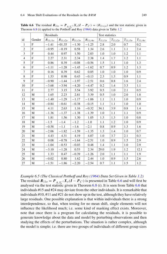
6.4 Mean Shift Evaluations of the Residuals in the BRM 249
Table 6.6 The residual R11o = PA,S−1
oXo(I − P C′ ) = (R11;ijo) and the test statistic given in
Theorem 6.8 (i) applied to the Potthoff and Roy (1964) data given in Table 1.2
Residuals Test statistics
id Gender R11;i1o R11;i2o R11;i3o R11;i4o T11;i1o T11;i2o T11;i3o T11;i4o
1 F −1.41 −01.35 −1.30 −1.25 2.8 2.0 0.7 0.2
2 F −0.95 −0.19 0.58 1.34 2.6 1.1 1.1 2.4
3 F 0.44 0.97 1.50 2.03 1.0 1.0 1.2 1.1
4 F 2.27 2.31 2.34 2.38 1.4 1.7 1.2 1.1
5 F 0.86 0.39 −0.08 −0.56 1.5 1.1 1.0 1.3
6 F −1.11 −1.28 −1.45 −1.62 0.7 0.9 1.2 1.3
7 F 0.16 0.39 0.62 0.85 1.0 1.0 1.0 0.9
8 F 1.53 0.98 0.43 −0.13 2.3 1.3 0.9 1.1
9 F −0.90 −1.44 −1.97 −2.51 0.6 0.8 1.6 2.4
10 F −3.68 −3.94 −4.20 −4.47 0.2 1.4 3.3 1.1
11 F 2.77 3.15 3.54 3.92 0.5 1.0 2.1 0.5
12 M 1.65 2.23 2.81 3.39 0.5 1.0 2.0 1.8
13 M −1.40 −1.29 −1.17 −1.06 1.1 1.1 1.0 0.9
14 M −0.84 −0.61 −0.38 −0.15 1.1 1.1 1.0 1.0
15 M 4.11 2.63 1.16 −0.32 34.1 3.9 0.8 1.4
16 M −1.36 −1.37 −1.38 −1.39 1.0 1.1 1.1 0.9
17 M 1.81 1.56 1.30 1.05 1.3 1.3 1.0 0.8
18 M −1.5 −1.4 −1.2 −1.0 1.1 1.2 1.0 0.9
19 M −0.58 −1.1 −1.6 −2.1 0.8 0.9 1.3 1.6
20 M −2.06 −1.82 −1.59 −1.35 1.3 1.4 1.0 0.7
21 M 4.43 4.31 4.19 4.07 1.0 3.7 2.1 0.3
22 M 0.08 −0.78 −1.64 −2.51 1.0 0.9 1.5 2.9
23 M −1.04 −0.53 −0.03 0.48 1.4 1.1 1.0 2.9
24 M −3.10 −1.28 0.53 2.34 29.0 1.9 1.2 12.1
25 M 1.33 0.47 −0.39 −1.26 2.0 1.1 1.1 1.9
26 M −0.02 0.80 1.62 2.44 1.0 0.9 1.5 2.6
27 M −1.51 −1.86 −2.20 −2.54 0.7 1.1 1.5 1.2
Example 6.5 (The Classical Potthoff and Roy (1964) Data Set Given in Table 1.2)The residual R11o = P
A,S−1o
Xo(I − P C ′) is presented in Table 6.6 and will first beanalysed via the test statistic given in Theorem 6.8 (i). It is seen from Table 6.6 thatindividuals #15 and #24 may deviate from the other individuals. It is remarkable thatindividuals #10, #11 and #21 do not show up in the test, although they have relativelylarge residuals. One possible explanation is that within individuals there is a stronginterdependence, so that, when testing for no mean shift, single elements will notinfluence the likelihood much; i.e. some kind of masking effect exists. Moreover,note that once there is a program for calculating the residuals, it is possible togenerate knowledge about the data and model by perturbing observations and thenstudying the effects of the perturbations. The situation is rather complex, althoughthe model is simple; i.e. there are two groups of individuals of different group sizes

250 6 Residuals
and for each group a separate model is assumed to hold. In addition to this, repeatedcorrelated observations are gathered. If we want to validate the model via a multipletesting procedure, it follows from Table 6.7 and the parametric bootstrap approachthat none of the residuals presented in Table 6.6 have a significant mean shift. Onecan artificially perturb the data to understand how large residuals should be in orderto have significant mean shifts.
In Table 6.8 the statements of Theorem 6.8 (ii) and (iii) have been appliedfor testing all the observations from an individual for a mean shift. Theorem 6.8(ii) concerns simultaneously testing for a mean shift within an individual andTheorem 6.8 (iii) assumes that the same mean shift appears within an individual.In the analysis, individuals #15, #21 and #24 are highlighted. However, accordingto Table 6.7 the mean shifts for these observations are not significant. ��
Table 6.7 Estimated quantiles for T11;ij1 , T11;ij2 and T11;ij3 corresponding to the test statisticsT11;ij1o, T11;ij2o and T11;ij3o (T11;ijo was presented in Theorem 6.8 (i)) as well as for T11;iko and
T 11;iko, k = 1, 2 (T11;io and T 11;io were given in Theorem 6.8 (ii), and (iii), respectively)
Quantile T11;ij1o T11;ij2o T11;ij3o T11;i1o T11;i2o T 11;i1o T 11;i2o
100% max 5.8×10¹¹ 8.9×10⁷ 1.2×10⁷ 1.5×10¹⁶ 1.3×10¹⁰ 1.7×10¹⁵ 1.7×10¹⁵
99% 1.8×10⁵ 5.2×10³ 5.3×10² 1.1×10⁷ 8.7×10⁴ 1.2×10⁶ 1.2×10⁶
95% 1.9×10³ 2.5×10² 65.4 2.1×10⁴ 9.0×10² 1.0×10³ 5.1×10²
90% 3.4×10² 77.2 29.9 1.9×10³ 1.7×10³ 1.7×10² 54.6
75% 55.5 20.3 11.6 1.8×10² 42.2 35.5 12.4
50% 17.4 9.0 6.3 44.9 17.3 12.7 6.1
25% 8.5 5.5 4.2 18.8 9.6 6.5 3.8
10% 5.5 3.9 3.2 10.8 6.4 4.1 2.8
5% 4.4 3.3 2.8 8.1 5.2 3.3 2.4
1% 3.1 2.6 2.3 5.1 3.7 2.4 1.9
0% min 2.0 2.0 1.8 2.5 2.1 1.1 1.1
The estimated quantiles are based on 10,000 simulations
Table 6.8 The data in Table 6.1 are analysed and the test statistic for column-wise mean shift,T11;io, based on Theorem 6.8 (ii), is presented
Individual
1 2 3 4 5 6 7 8 9 10 11 12 13 14
T11;io 2.1 2.4 1.4 3.1 1.9 1.3 1.0 2.6 2.4 9.2 7.6 3.8 1.3 1.1
T 11;io 1.9 1.9 1.4 3.2 1.1 1.1 1.1 1.3 1.1 6.4 8.1 2.4 1.3 1.1
Individual
15 16 17 18 19 20 21 22 23 24 25 26 27
T11;io 45.9 1.4 1.6 1.4 1.8 1.8 20.7 3.1 1.5 93.5 2.8 2.8 2.1
T 11;io 2.5 1.4 1.5 1.3 1.3 1.7 20.5 1.2 1.0 1.2 1.0 1.2 1.8
The test statistic for column-wise mean shift, T 11;io, based on Theorem 6.8 (iii), is also shown

6.5 Residual Analysis for R1 in the BRM 251
6.5 Residual Analysis for R1 in the BRM
So far R11 and R12 have been exploited. However, since these residuals are notindependently distributed, it can be worthwhile performing a residual analysis of
R1 = X(I − P C ′) = R11 + R12.
Because R1 ∼ Np,n(0,�, I − PC ′), i.e. the distribution is known, this case shouldbe both simpler and more reliable than considering R11 and R12 separately, althoughR1 cannot completely contain the same amount of information as R11 and R12.Moreover, since R1 is also the residual in the MANOVA model, R1 has in factalready been considered in Sect. 6.1. Next some of the statements of Sect. 6.1 arerepeated, but the idea now is to carry out the presentation, although very briefly,relatively systematically in line with the treatments of R11 and R12. Let
I − P C ′ = V V ′, V : n × n1, n1 = n − r(C)),
and by post-multiplying R1 one eliminates the singularity, i.e.
RN1 = R1L1, L1 = V (V ′V )−1. (6.37)
Now Definition 6.2 and Theorem 6.8 are adjusted so that the presentation fits RN1 .
The results of the theorem will, however, not be proved, since all the results areobtained by simply copying the results presented in earlier sections.
Definition 6.3 Models and notation are presented for the likelihood functionsrelated to R1 = X(I − P C ′); these models and this notation are used when testingfor mean shifts under the conditions given in (6.36):
(a) RN1;ij = dj θe′
iL1 + E1, RN1;ijo = R1oL1;
(b) RN1;i = θe′
iL1 + E1, RN1;io = R1oL1;
(c) RN1;i = 1θe′
iL1 + E1, RN1;io = R1oL1;
(d) RN1;j = dj θ1′L1 + E1, RN
1;jo = R1oL1;
E1 ∼ Np,n1(0,�, I ), n1 = n − r(C), L1 is defined by (6.37), and dj and ei areunit basis vectors.

252 6 Residuals
Denote the observed value of R1 by R1o. Moreover, R1;ijo, R1;io and R1;jo are allequal to R1o, given in Definition 6.1, and as before the subscripts ij , i and j onlyindicate which type of mean shift and which element is being studied.
Theorem 6.9 In Definition 6.3, in order to test for no mean shift in the residualR1,models with four types of mean shift were presented. The test statistics for the fourtypes are presented below.
(i) Let the model and mean shift be as in Definition 6.3 (a). The test statistic forRN
1;ij , testing for no mean shift, is given by
T1;ijo =(n − r(C) − 1)d ′
jR1o(I − PC ′)ei (e
′i(I − PC ′)ei )
−1e′i(I − PC ′)R′
1odj
d ′jR1o(I − PC ′)(I − ei (e
′i (I − PC ′)ei )
−1e′i )(I − PC ′)R′
1odj
.
(ii) Let the model and mean shift be as in Definition 6.3 (b). Then the test statisticfor RN
1;i , testing for no mean shift, is given by
T1;io = |R1o(I − PC ′)R′1o|
|R1o(I − P C ′)(I − ei (e′i (I − P C ′)ei )−1e′
i )(I − P C ′)R′1o|
.
(iii) Let the model and mean shift be as in Definition 6.3 (c). Then the test statisticfor R1, testing for no mean shift, is given by
T 1;io = (n − r(C) − 1)1′R1o(I − PC′)ei (e′i (I − P C′)ei )
−1e′i (I − PC′)R′
1o1
1′R1o(I − PC′)(I − ei (e′i (I − PC′)ei )−1e′
i )(I − PC′)R′1o1
.
(iv) Let the model and mean shift be as in Definition 6.3 (d). Then the test statisticfor R1, testing for no mean shift, is given by
T 1;jo = (n − r(C) − 1)d ′jR1o(I − P C′ )1n(1′
n(I − P C′ )1n)−11′
n(I − P C′ )R′1odj
d ′jR1o(I − P C′ )(I − 1n(1′
n(I − P C′ )1n)−11′n)(I − P C′ )R′
1odj
.
Proof Since I − P C ′ is idempotent, L1 in (6.37) equals V because V is a semi-orthogonal matrix, i.e. V ′V = I n1 . Moreover, note that all the models of thetheorem are of the form
XV = μV + E1, E1 ∼ Np,n1(0,�, I ),
where μ equals dj θe′i , θe′
i , 1θe′i or dj θ1′. This is a standard MANOVA model with
bilinear restrictions on the mean and the results will be verified in detail in the nextsection under more general assumptions. ��
To understand best what may occur when performing data analysis, once againthe Potthoff and Roy (1964) data set is used. It is also of particular interest to

6.5 Residual Analysis for R1 in the BRM 253
Table 6.9 Estimated quantiles for T1;ij1 , T1;ij2 and T1;ij3 connected to the test statistics T1;ij1o,T1;ij2o and T1;ij3o (with T1;ijo defined in Theorem 6.9 (i)) are given, and applied to the Potthoffand Roy data set presented in Table 1.2
Quantile T1;ij1o T1;ij2o T1;ij3o R12;ij1o R12;ij2o R12;ij3o
100%max 45.6 25.2 17.5 11.1 9.2 8.8
99% 21.7 14.2 10.8 8.6 7.3 6.6
95% 16.2 11.1 8.6 7.6 6.6 6.0
90% 13.9 9.7 7.8 7.1 6.2 5.7
75% 11.1 8.1 6.7 6.4 5.6 5.2
50% 8.8 6.9 5.8 5.7 5.1 4.8
25% 7.3 5.9 5.1 5.2 4.6 4.4
10% 6.3 5.2 4.6 4.7 4.3 4.0
5% 5.8 4.9 4.4 4.5 4.1 3.8
1% 5.0 4.3 3.9 4.1 3.7 3.5
0% min 4.0 3.4 3.1 3.4 3.2 3.1
Estimated quantiles are given for the three largest (by absolute value) residuals, R1ij ko, k = 1, 2, 3,obtained from the same data set. The estimated quantiles are based on 10,000 simulations
compare the results for R1 with those for R11 and R12 to determine whether thereis any significant advantage in decomposing R1 (Table 6.9).
Example 6.6 (The Classical Potthoff and Roy (1964) Data Set Given in Table 1.2)The residual R1o = Xo(I − P C ′) is presented in Table 6.10. Also shown in this
table are the values of the test statistic of Theorem 6.9 (i). It can be observed thatindividuals #10, #11, #21 and #24 differ from the other individuals, with the largestvalue for individual #24 when j = 1, i.e. at age 8. However, from Table 6.9 itfollows that no residuals have a significant mean shift, i.e. even the value T1;241o =9.0 is not significant.
Since there seem to be some individuals which deviate from the rest, we nowtest for a mean shift for a whole individual or for an equal mean shift for a wholeindividual. The results are presented in Table 6.11. For T1;io only individual #20seems to stand out, whereas according to T 1;io, individuals #10, #11 and #21 shouldbe investigated. The appropriate distributions for decision making are presented inTable 6.12 and it is T1;201o = 5.2 which exhibits a mean shift which is significant,as well as T 1;113o = 4.6. The last result is interesting, but difficult to interpret, sinceneither T 1;111o nor T 1;112o are significant. Therefore, the final conclusion from theresidual analysis for the residual R1 and the split R1 = R11 + R12 is that only theresidual from individual #20 is too far away from 0 to be deemed non-significant.
Now all the significant findings concerning R1 are hereby summarized. InTable 6.1 the observation T12;2031o was significant, as well as R12;2031o. Moreover, inTable 6.3 the statistics T12;201o = 9379.2 and T 12;201o = 9486.7 were significant.Tables 6.6 and 6.8 give indications that observations or individuals deviate, butthe overall conclusion is that no elements in R11, with its mean shift, deviate

254 6 Residuals
Table 6.10 The residual R1o = Xo(I − P C′ ) = (R1;ijo) and the test statistic given inTheorem 6.9 (i) applied to the Potthoff and Roy (1964) data presented in Table 1.2
Residuals Test statistics
id Gender R1;i1o R1;i2o R1;i3o R1;i4o T1;i1o T1;i2o T1;i3o T1;i4o
1 F −0.18 −2.23 −1.59 −1.09 0.0 1.3 0.4 0.3
2 F −0.18 −0.73 0.91 1.41 0.0 0.1 0.1 0.4
3 F −0.68 1.77 1.41 1.91 0.1 0.8 0.3 0.8
4 F 2.32 2.27 1.91 2.41 1.1 1.4 0.6 1.3
5 F 0.32 0.77 −0.59 −0.59 0.0 0.2 0.1 0.1
6 F −1.18 −1.23 −2.09 −1.59 0.3 0.4 0.7 0.5
7 F 0.32 0.27 −0.09 0.91 0.0 0.0 0.0 0.2
8 F 1.82 0.77 0.41 −0.09 0.7 0.2 0.0 0.0
9 F −1.18 −1.23 −1.09 −2.59 0.3 0.4 0.2 1.5
10 F −4.68 −3.23 −4.09 −4.59 5.2 3.0 3.1 5.5
11 F 3.32 2.77 4.91 3.91 2.4 2.1 4.7 3.7
12 M 3.12 1.19 3.28 3.53 2.0 0.4 1.8 2.9
13 M −1.38 −1.31 −2.72 −0.97 0.3 0.4 1.2 0.2
14 M 0.12 −1.31 −1.72 0.03 0.0 0.4 0.5 0.0
15 M 2.62 3.69 0.78 −0.47 1.4 3.9 0.1 0.0
16 M −2.88 −0.31 −3.22 −1.47 1.7 0.0 1.8 0.5
17 M 1.62 1.69 1.28 1.03 0.5 0.7 0.3 0.2
18 M −0.88 −1.81 −1.22 −0.97 0.1 0.8 0.2 0.2
19 M 1.12 −2.31 −1.22 −1.97 0.2 1.4 0.2 0.8
20 M 0.12 −3.31 5.28 −1.47 0.0 3.0 5.4 0.5
21 M 4.62 4.19 5.28 4.03 4.9 5.2 5.4 3.9
22 M 0.12 −0.81 −2.22 −2.47 0.0 0.2 0.8 1.3
23 M −1.38 −0.31 −1.72 0.53 0.4 0.0 0.5 0.1
24 M −5.88 0.69 0.28 2.03 9.0 0.1 0.0 0.9
25 M −0.38 1.69 −0.22 −1.47 0.0 0.7 0.0 0.5
26 M 0.12 0.69 0.28 2.53 0.0 0.1 0.0 1.4
27 M −0.88 −2.31 −2.22 −2.47 0.1 1.4 0.8 1.3
significantly from 0. For R1 = R11 +R12, the results were presented in Tables 6.10and 6.11, and it was concluded that only individual #20 had a significant meanshift. Thus, it can be stated that only individual #20 had a large residual, which tosome extent can also be seen in an ocular data inspection. Finally we claim thatthe residual analysis has shown that if one just observes data without referringto distributions and probability statements, it is difficult to determine how largedeviating values should be to be deemed as outlying (extreme) observations. ��
In the residual analysis so far, the residual R1 has been scrutinized; i.e. theresidual has been decomposed and various mean shift tests have been performed.Now R2o = (I − P A,So)XoPC ′ is considered. As noted before, R2 is suitablefor validating the model, but is not connected to single observations or columns inX. In Theorem 6.7 it was noted that R2 has the same distribution as R2N − U2.

6.5 Residual Analysis for R1 in the BRM 255
Table 6.11 The data in Table 6.10 are analysed and the test statistic for column-wise mean shift,T1;io, based on Theorem 6.9 (ii), is presented
Individual
1 2 3 4 5 6 7 8 9 10 11 12 13 14
T1;io 1.1 1.1 1.1 1.1 1.0 1.0 1.0 1.0 1.1 1.3 1.2 1.2 1.1 1.1
T 1;io 0.5 0.0 0.3 1.5 0.0 0.7 0.0 0.1 0.7 6.0 4.6 2.3 0.7 0.1
Individual
15 16 17 18 19 20 21 22 23 24 25 26 27
T1;io 1.6 1.1 1.0 1.0 1.2 5.2 1.3 1.1 1.1 2.7 1.3 1.1 1.1
T 1;io 0.8 1.1 0.5 0.4 0.3 0.0 7.2 0.5 0.1 0.1 0.0 0.2 1.1
The test statistic for column-wise mean shift, T 1;io, based on Theorem 6.9 (iii), is also shown
Table 6.12 Estimated quantiles connected to the test statistics T1;iko and T 1;iko, respectively,defined in Theorem 6.9 (ii) and (iii), are presented for the Potthoff and Roy (1964) data givenin Table 1.2
Quantile T1;i1o T1;i2o T1;i3o T 1;i1o T 1;i2o T 1;i3o
100% max 3.7 2.4 2.0 34.4 10.6 6.9
99% 2.5 1.9 1.7 17.4 7.6 5.1
95% 2.2 1.8 1.6 12.3 6.3 4.4
90% 2.0 1.7 1.5 10.4 5.6 4.0
75% 1.8 1.6 1.5 8.0 4.8 3.5
50% 1.7 1.5 1.4 6.1 4.0 3.0
25% 1.6 1.5 1.4 4.9 3.4 2.6
10% 1.5 1.4 1.4 4.1 3.0 2.3
5% 1.5 1.4 1.3 3.7 2.8 2.2
1% 1.4 1.4 1.3 3.2 2.4 1.8
0% min 1.3 1.3 1.3 2.2 1.8 1.1
The estimated quantiles are based on 10,000 simulations
The approximating density fKR2NL(KR0L) is utilized for specific K and L, andD[R2N ] is decomposed spectrally, i.e.
D[R2N ] = V V ′ ⊗ WW ′, V : n × r(C), W : p × (p − r(A)),
which follows from �PAo,−1 = WW ′ and PC ′ = V V ′. In the same way as RN12
was introduced, let
RN2;ij = KR2L, K = (W ′W )−1W ′, L = V (V ′V )−1,
and then with these choices of K and L in Theorem 6.7, a non-singular densityapproximation exists. The model for testing for a mean shift, e.g. following (6.21),is written as
RN2;ij = Kdj θe′
iL + E2, dj : p × 1, ei : r(C) × 1, (6.38)

256 6 Residuals
where E2 has the approximating density given in Theorem 6.7. The density dependson �, but if one replaces it by �, given in Theorem 3.1, or by �U , given inTheorem 4.7, we have a complete specification of the likelihood and can formulatethe following test quantity for H0 : θ = 0 versus H1 : θ �= 0:
T2;ijo = LN2;qij (
θo)
LN2;ij
, (6.39)
where LN2;ij is the likelihood for RN
2 under H0 and RN2 (θo) under H1 with θo =
d ′jR2oei . Moreover, a parallel discussion of testing for mean shifts via
RN2;i = Kθe′
iL + E2,
RN2;i = K1θe′
iL + E2,
RN2;j = Kdj θ1′L + E2
follows the same ideas as before; RN2;i and RN
2;j are identical to RN2 . However, one
should remember that r(C) is often a small value, meaning that there are only afew independent observations available, and therefore formal tests usually have lowpower.
6.6 Residuals for the EBRM3B
In this section the basis for studying residuals for the EBRM3B is given. Figure 2.7
presented a decomposition of the whole tensor space showing the characteristic“stairs structure”. The next figure (Fig. 6.4) once again shows the spaces, but nowthe focus is directed on the residuals.
In Fig. 6.4, for any given �, ten different residuals are presented. All theseresiduals can be studied, as well as linear combinations of them. In a textbook thisis impossible and only the following four residuals will be highlighted:
(i) R1N = R11 + R12 + R13 + R14;(ii) R2N = R21 + R22 + R23;
(iii) R3N = R31 + R32;(iv) R4N = R4N .
Explicit expressions for any given � can be obtained by projecting X on Wi ⊗ Vj ,i ≤ j , i.e. vecR5−i,j = (PWi
⊗ PVj ,)vecX, where Wi and Vj are defined inFig. 6.4. However, � is unknown and then the inner product has to be estimated.Therefore, the residual analysis will rest on Corollary 3.3, i.e. X − E[X] will be

6.6 Residuals for the EBRM3B 257
Fig. 6.4 Decomposition ofthe whole space according tothe within-individuals and thebetween-individuals designs,illustrating the mean andresidual spaces in EBRM3
B :V1 = C(A1), V2 = C(A1 :A2) ∩ C(A1)
⊥,V3 = C(A1 : A2 :A3) ∩ C(A1 : A2)
⊥,V4 = C(A1 : A2 : A3)
⊥,W1 = C(C ′
3),W2 = C(C ′
2) ∩ C(C′3)
⊥,W3 = C(C ′
1) ∩ C(C′2)
⊥,W4 = C(C ′
1)⊥
considered. The fact will be utilized that (using the notations of Theorem 3.2)
X − E[X] = X − P A1,S1XP C ′1− P
Q′1A2,S2
XP C ′2− P
Q′2Q′
1A3,S3XP C ′
3
= X(I − P C ′1) + (I − P A1,S1)X(P C ′
1− P C ′
2)
+(I − P A1,S1 − PQ′
1A2,S2)X(PC ′
2− PC ′
3)
+(I − P A1,S1 − PQ′
1A2,S2− P
Q′2Q′
1A3,S3)XP C ′
3.
Thus, since C(I − P C ′1) = W4, C(PC ′
1− P C ′
2) = W3, C(PC ′
2− P C ′
3) = W2 and
C(PC ′3) = W1, the next definitions make sense.
Definition 6.4 Let Qi , S1 andSi , i = 2, 3, be as in Theorem 3.2. For the EBRM3B
the following residuals will be considered:
(i) R1 = X(I − PC ′1);
(ii) R2 = (I − P A1,S1)X(P C ′1− P C ′
2);
(iii) R3 = (I − P A1,S1 − PQ′
1A2,S2)X(P C ′
2− P C ′
3);
(iv) R4 = (I − P A1,S1 − PQ′
1A2,S2− P
Q′2Q′
1A3,S3)XP C ′
3.
Note that the residual R1 is identical to R1 ∼ Np,n(0,�, I − PC ′1) for the
BRM and, therefore, for R1 only the mean shift test of the residual analysiswill be provided. Missing details can be found in Sect. 6.2. However, it should beremembered that in many applications only the residual in Definition 6.4 (i) bearsenough information to be analysed in detail, for example via statistical tests. Thisdoes not mean that R2, R3 and R4 should be discarded, but it may happen thatfor these residuals there is only enough information available for presenting some

258 6 Residuals
graphs which can be ocularly inspected. Note that R1 concerns how independentobservations relate to the other independent observations, whereas R2, R3 andR4 all consider how the model fits the data. For example, if one’s intention is todetermine whether a second or third degree polynomial growth model fits one ofseveral treatment groups, then the residuals can be supportive.
In Definition 6.4 the projections are performed with the help of inner products.Due to the estimation procedure, different projections have different inner products.However, since
A′1S
−13 = A′
1S−11 , A′
2Q1
S−13 = A′
2Q1
S−12 ,
all residual projections can be considered to take place on spaces where the innerproduct defined via S3 is used, i.e. R2 = (I − P A1,S3
)X(P C ′1
− P C ′2), R3 =
(I − PA1,S3− P
Q′1A2,S3
)X(PC ′2
− PC ′3) and R4 = (I − P A1,S3
− PQ′
1A2,S3−
PQ′
2Q′
1A3,S3)XP C ′
3. Moreover, instead of S3 the MLE �, given by Theorem 3.2,
could have been used without any difference in the performed projections.Concerning the stochastic properties of the residuals the basic relations which
will be utilized are the following:
• S1 is independent of X(P C ′1− P C ′
2), X(PC ′
2− PC ′
3) and XP C ′
3;
• S2 is independent of X(P C ′2− P C ′
3) and XP C ′
3;
• S3 is independent of XP C ′3.
Applying these properties it can be shown that
E[R2] = E[R3] = E[R4] = 0.
The result follows from the fact that
(I − P A1,S1 − PQ′
1A2,S2)A2 = 0,
(I − P A1,S1 − PQ′
1A2,S2− P
Q′2Q′
1A3,S3)A3 = 0.
The next theorem is a direct consequence of the above-mentioned independencerelations and the detailed moment calculations performed in Chap. 4. It is based onthe fact that the following alternative expressions for the residuals can be obtained(Gi , W i and Z1,s are defined in Table 4.1):
R2 = P ′G1,W
−11
X(P C ′1− P C ′
2) = Q
′1X(PC ′
1− PC ′
2)
= Z1,1X(P C ′1− PC ′
2), (6.40)
R3 = P ′G1,W
−11
P ′G2,W
−12
X(P C ′2− P C ′
3) = Q
′2Q
′1X(P C ′
2− P C ′
3)
= Z1,2X(P C ′2− PC ′
3), (6.41)
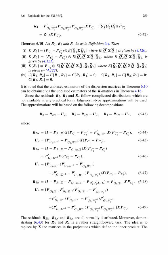
6.6 Residuals for the EBRM3B 259
R4 = P ′G1,W
−11
P ′G2,W
−12
P ′G3,W
−13
XPC ′3
= Q′3Q
′2Q
′1XP C ′
3
= Z1,3XP C ′3. (6.42)
Theorem 6.10 Let R2, R3 and R4 be as in Definition 6.4. Then
(i) D[R2] = (P C ′1−PC ′
2)⊗E[Q′
1�Q1], where E[Q′
1�Q1] is given by (4.120);
(ii) D[R3] = (P C ′2
− PC ′3) ⊗ E[Q′
2Q
′1�
Q1Q2], where E[Q′
2Q
′1�
Q1Q2] is
given by (4.121);(iii) D[R4] = PC ′
3⊗ E[Q′
3Q
′2Q
′1�
Q1Q2
Q3], where E[Q′3Q
′2Q
′1�
Q1Q2
Q3]is given by (4.122);
(iv) C[R1,R2] = C[R1,R3] = C[R1,R4] = 0; C[R2,R3] = C[R2,R4] = 0;C[R3,R4] = 0.
It is noted that the unbiased estimators of the dispersion matrices in Theorem 6.10can be obtained via the unbiased estimators of the K-matrices in Theorem 4.16.
Since the residuals R2, R3 and R4 follow complicated distributions which arenot available in any practical form, Edgeworth-type approximations will be used.The approximations will be based on the following decompositions:
R2 = R2N − U2, R3 = R3N − U 3, R4 = R4N − U4, (6.43)
where
R2N = (I − P A1,)X(P C ′1− P C ′
2) = P ′
G1,−1X(P C ′1− P C ′
2), (6.44)
U 2 = (P ′G1,
−1 − P ′G1,W
−11
)X(PC ′1− PC ′
2), (6.45)
R3N = (I − P A1, − PQ′1A2,
)X(PC ′2− P C ′
3)
= P ′G2,
−1X(P C ′2− P C ′
3), (6.46)
U 3 = (
P ′G1,
−1(P′G2,
−1 − P ′G2,W
−12
)
+(P ′G1,−1 − P ′
G1,W−11
)P ′G2,W
−12
)
X(PC ′2− P C ′
3), (6.47)
R4N = (I − P A1, − PQ′1A2,
− P Q′2Q
′1A3,
) = P ′G3,−1XP C ′
3, (6.48)
U 4 = (
P ′G1,−1P
′G2,−1(P
′G3,−1 − P ′
G3,W−13
)
+P ′G1,−1(P
′G2,−1 − P ′
G2,W−12
)P ′G3,W
−13
+(P ′G1,
−1 − P ′G1,W
−11
)P ′G2,W
−12
P ′G3,W
−13
))
XP C ′3. (6.49)
The residuals R2N , R3N and R4N are all normally distributed. Moreover, demon-strating (6.43) for R3 and R4 is a rather straightforward task. The idea is toreplace by � the matrices in the projections which define the inner product. The

260 6 Residuals
decomposition of R2 is trivial. For R3 it is noted that
P ′G1,W
−11
P ′G2,W
−12
= P ′G1,−1P
′G2,−1
−P ′G1,
−1(P′G2,
−1 − P ′G2,W
−12
) − (P ′G1,
−1 − P ′G1,W
−11
)P ′G2,W
−12
and P ′G1,−1P
′G2,−1 = P ′
G2,−1 . Moreover, concerning R4, calculations appliedto R3 yield
P ′G1,W
−11
P ′G2,W
−12
P ′G3,W
−13
= P ′G1,
−1P′G2,
−1P′G3,
−1
−P ′G1,−1P
′G2,−1(P
′G3,−1 − P ′
G3,W−13
)
−P ′G1,−1(P
′G2,−1 − P ′
G2,W−12
)P ′G3,W
−13
−(P ′G1,−1 − P ′
G1,W−11
)P ′G2,W
−12
P ′G3,W
−13
and P ′G1,−1P
′G2,−1P
′G3,−1 = P ′
G3,−1 .Hence, the approximating quantities R2N , R3N and R4N have been established.
To validate if they make sense, it will be shown that E[U i] = 0 and C[RiN ,U i ] =0, i = 2, 3, 4. Concerning the expectation, E[U i ] = E[RiN ] + E[Ri ] = 0. Forthe covariance it is noted that (see also Theorem B.21 (viii) in Appendix B and itsproof)
E[PG1,W−1
1] = P G1,−1, E[P
G2,W−12
] = P G2,−1, E[PG3,W−1
3]= PG3,−1,
E[PG3,W−1
3P
G2,W−12
] = P G3,−1, E[Z′1,s] = P Gs,−1 ,
which, if one applies one or more of these results directly to C[RiN ,U i ], i = 1, 2, 3,will show that the covariance equals 0. For example,
C[R3N,U 3] = (P C ′2− P C ′
3) ⊗
{
E[P ′G2,−1�(P G2,−1 − P
G2,W−12
)PG1,−1 ]
+ E[P ′G2,−1�P
G2,W−12
(P G1,−1 − PG1,W
−11
)]}
= 0,
since
E[(PG2,−1 − PG2,W
−12
)] = 0,
E[PG2,W
−12
(P G1,−1 − P
G1,W−11
)] = P G2,−1 − P G2,
−1 = 0.
With these calculations, the preparations for presenting Edgeworth-type approxi-mations are now completed. The first result concerns R2 and it is given in the nexttheorem.

6.6 Residuals for the EBRM3B 261
Theorem 6.11 The distribution of the residual R2, given in (6.40), can be approx-imated through the difference
R2 = R2N − U 2,
where R2N and U 2 are defined by (6.44) and (6.45), respectively. Let K: p1 × p
and L: n × n1, both of which are known, and
KR2NL ∼ Np1,n1(0,K�PAo1,−1K ′,L′(P C ′
1− P C ′
2)L).
Then an Edgeworth-type expansion fKR2EL(KRoL) of the density of KR2L, viathe density of KR2NL, assuming D[KR2NL] is p.d., is given by
fKR2EL(KRoL) = {
1 − 12
p−r(A1)n−r(C1)−p+r(A1)−1n1tr{KP A1,�K ′(K�PAo
1,−1K ′)−1}+ 1
2p−r(A1)
n−r(C1)−p+r(A1)−1 tr{(K�P Ao1,−1K ′)−1KP A1,�K ′(K�PAo
1,−1K ′)−1
× KRoL(L′(I − PC′)L)−1L′R′oK
′}}fKR2NL(KRoL).
Proof The proof follows by applying Corollary 5.3, Theorem 6.10 and (4.120). ��Using Appendix B, Theorem B.23 (i) gives the dispersion of the approximatingdistribution.
Corollary 6.4 LetKR2EL be defined via fKR2EL(KRoL), given in Theorem 6.11,where it is assumed that fKR2EL(KRoL) ≥ 0. Then
(i) E[KR2EL] = 0;(ii) D[KR2EL] = L′(I − P C ′)L ⊗ K(�PAo
1,−1 + g1,1P A1,�)K ′,where g1,1 is given in Theorem 4.15.
Similar results to those presented above for R2 are now given for R3.
Theorem 6.12 The distribution of the residual R3, given in (6.41), can be approx-imated through the difference
R3 = R3N − U 3,
where R3N and U 3 are defined by (6.46) and (6.47), respectively. Let K: p1 × p
and L: n × n1, both of which are known, and
KR3NL ∼ Np1,n1(0,K�P G′2,
−1K ′,L′(PC ′2− PC ′
3)L).

262 6 Residuals
Then an Edgeworth-type expansion fKR3EL(KRoL) of the density of KR3L, viathe density of KR3NL, under the assumption that D[KR3NL] is p.d., is given by
fKR3EL(KRoL) = {
1 − 12n1tr{K(g1,2K1 + g2,2K2)K
′(K�P G2,−1K′)−1}
+ 12 tr
{
(K�P G2,−1K ′)−1K(g1,2K1 + g2,2K2)K
′(K�PG2,−1K ′)−1
× KRoL(L′(P C ′2− P C ′
3)L)−1L′R′
oK′}}fKR3N L(KRoL),
where gi,2 is defined in Theorem 4.15 and K i , i = 1, 2, in Theorem 4.12.
Corollary 6.5 LetKR3EL be defined via fKR3EL(KRoL), given in Theorem 6.12,where it is assumed that fKR3EL(KRoL) ≥ 0. Then
(i) E[KR3EL] = 0;(ii) D[KR3EL] = L′(PC ′
2− PC ′
3)L ⊗ K(�PG2,
−1 + g1,2K1 + g2,2K2)K′.
Finally, R4 is considered.
Theorem 6.13 The distribution of the residual R4, given in (6.42), can be approx-imated through the difference
R4 = R4N − U 4,
where R4N and U 4 are defined by (6.48) and (6.49), respectively. Let K: p1 × p
and L: n × n1, both of which are known, and
KR4NL ∼ Np1,n1(0,K�PG′3,
−1K ′,L′PC ′3L).
Then an Edgeworth-type expansion fKR4EL(KRoL) of the density of KR4L, viathe density of KR4NL, under the assumption that D[KR4NL] is p.d., is given by
fKR4EL(KRoL) = {
1 − 12n1tr{K(g1,3K1 + g2,3K2 + g3,3K3)K
′(K�PG3,−1K ′)−1}
+ 12 tr
{
(K�P Ao,−1K′)−1K(g1,3K1 + g2,3K2 + g3,3K3)K
′(K�PAo,−1K′)−1
× KRoL(L′PC′3L)−1L′R′
oK′}}fKR4NL(KRoL),
where gi,3 is defined in Theorem 4.15 and K i , i = 1, 2, 3, in Theorem 4.12.
Corollary 6.6 LetKR4EL be defined via fKR4EL(KRoL), given in Theorem 6.13,where it is assumed that fKR4EL(KRoL) ≥ 0. Then
(i) E[KR4EL] = 0;(ii) D[KR4EL] = L′PC ′
3L ⊗ K(�P G3,−1 + g1,3K1 + g2,3K2 + g3,3K3)K
′.
Hence, a basis for validating the residuals in the EBRM3B has been established.
As for the BRM , it is suggested that the validation should be carried out via meanshift tests. For the BRM five different tests have been suggested, see Sect. 6.1,

6.6 Residuals for the EBRM3B 263
although details have not been given for all of them. Here we have four differentresiduals and the task of constructing most of the possible alternative tests is left tothe reader. The case which will be treated here is that where the mean shift is of theform dj θe′
i .Consider R1 = X(I − PC ′
1), which bears information on how columns
(individuals) deviate from the average of the columns (individuals). The residualR1 is identical to R1 for the BRM , and all BRM-results connected to R1 can becopied. First we have to eliminate the singularity (see (6.37)), and thereafter the teststatistic is presented which corresponds to the mean shift hypothesis in Theorem 6.9.As before, the parametric bootstrap is suggested for evaluating which elements inR1 are truly large.
Turning to R2, we also have a very similar quantity to R2, obtained from a BRM
and presented in Definition 6.1 (ii). Thus, with minor modifications, i.e. changingP C ′ to P C ′
1− PC ′
2= P QC ′
2, Q = I − P C ′
1, one can use the same ideas as those
used for the BRM and the same results as those obtained for the BRM . Whenfurther considering R3 and R4, one can use the same statistic as was used for R2,since the approximate likelihood in all cases will be of the same form. For example,see Theorems 6.11–6.13 and note that nothing unexpected happens when movingfrom R2 to R3 or R4. Thus, in the next theorem we can immediately summarize theappropriate test statistics for a relatively detailed residual analysis of the EBRM3
B .The same notation will be adopted as that used when working with the BRM , i.e.
RNk;ij = Kdj θe′
iL + Ek, k = 1, 2, 3, 4.
The residual RNk;ij is the same as RN
k = KRkL, k = 1, 2, 3, 4, and, as before,
ij only indicates which element is supposed to have a mean shift, while RNk is
presented in (6.37) and (6.38) for k = 1 and k = 2, respectively, and for k = 3, 4it will be defined in the following. The vectors dj and ei are unit basis vectors, θ
is an unknown parameter, E1 ∼ Np,n1(0,�, I ), and Ei , i = 2, 3, 4, are definedthrough the densities in Theorems 6.11, 6.12 and 6.13, respectively. The matricesK and L depend also on k, k = 1, 2, 3, 4, and are chosen so that non-singulardistributions are obtained. Finally, it is noted that Tk;ijo, k = 1, 2, 3, 4, representsthe observed test statistic, LN
k;ij (θ) is the likelihood based on Ek, and as θ the
estimator θ = d ′jRkei is used, Lk;ij is the likelihood under H0, i.e. with no mean
shift, and Rko is the observed version of Rk . In the likelihood, both under H0and H1, the dispersion matrix has been replaced by �o, the maximum likelihoodestimate, given in Theorem 3.2.
Theorem 6.14 Consider Ri , i = 1, 2, 3, 4, given in Definition 6.4.
(i) For R1 let
RN1;ij = dj θe′
iL + E1, RN1;ij = R1L, L = V (V ′V )−1, (I − P C ′
1)=V V ′;
(V is of full rank), E1 ∼ Np,n1(0,�, In1).

264 6 Residuals
Then a test statistic for testing H0 : θ = 0 against H1 : θ �= 0 is given by
T1;ijo = (n − r(C1) − 1)d ′jR1o(I − P C′
1)ei (e
′i (I − PC′
1)ei )
−1e′i (I − P C′
1)R′
1odj
d ′jR1o(I − PC′
1)(I − ei (e
′i (I − PC′
1)ei )−1e′
i )(I − P C′1)R′
1odj
.
(ii) For R2 let
RN2;ij = Kdj θe′
iL + E2, RN2;ij = KR2L, K = (W ′W )−1W ′ L = V (V ′V )−1,
(W and V are of full rank), �PAo1,−1 = WW ′, PC ′
1− PC ′
2= V V ′;
E2 has the approximating density given in Theorem 6.11. Then a test statisticfor testing H0 : θ = 0 against H1 : θ �= 0 is given by
T2;ijo = LN2;ij (θo)
LN2;ij
,
where LN2;ij is the likelihood for RN
2 (obtained via E2) underH0 and LN2;ij (θo)
is obtained under H1, withθo = d ′jR2oei .
(iii) For R3 let
RN3;ij = Kdj θe′
iL + E3, RN3;ij = KR3L, K = (W ′W )−1W ′, L = V (V ′V )−1,
(W and V are of full rank), �PGo2,−1 = WW ′, P C′
2− P C′
3= V V ′;
E3 has the approximating density given in Theorem 6.12. Then a test statisticfor testing H0 : θ = 0 against H1 : θ �= 0 is given by
T3;ijo = LN3;ij (θo)
LN3;ij
,
where LN3;ij is the likelihood for RN
3 (obtained via E3) underH0 and LN3;ij (θo)
is the likelihood under H1 withθo = d ′jR30ei .
(iv) For R4 let
RN4;ij = Kdj θe′
iL + E4, RN4;ij = KR4L, K = (W ′W )−1W ′ L = V (V ′V )−1,
(W and V are of full rank), �PGo3,−1 = WW ′, PC′
3= V V ′;
E4 has the approximating density given in Theorem 6.13. Then a test statisticfor testing H0 : θ = 0 against H1 : θ �= 0 is given by
T4;ijo = LN4;ij (θo)
LN4;ij
,

6.6 Residuals for the EBRM3B 265
where LN4;ij is the likelihood for LN
4;ij (obtained via E4) underH0 and RN4 (θo)
is obtained under H1, withθo = d ′jR4oei .
To finalize the residual analysis, one has to take care of the large residuals,i.e. those residuals which significantly deviate from the other residuals, for examplewhen testing hypotheses. A pure data analysis approach is suggested for deter-mining the distribution of these large/largest residuals; i.e. Xo is simulated fromNp,n1(0,�o, I ), which can then be used to generate the residuals and therebythe largest values of the residuals, as well as the distributions of the large/largestresiduals. The estimate �o is for example the observed maximum likelihoodestimator, presented in Theorem 3.2.
This section is concluded by an example which shows how the residuals Ri ,i = 1, 2, 3, 4, can be utilized when evaluating an EBRM3
B .
Example 6.7 In this example the aim is to demonstrate how outlying observationswill show up in the residuals Ri , i = 1, 2, 3, 4, presented in Definition 6.4, andnot to present a residual analysis where the distribution of the largest residuals isinvestigated. The approach is completely in line with what was performed with theBRM . Consider the model presented in Example 1.9. Based on the given design andparameter matrices, a data matrix X: 10×45 can be generated. Here in Example 6.7some values are replaced by outlying observations. The effect of the contaminationis studied with the help of the absolute difference mk;ij , defined as
mk;ij = |d ′j (˜Rko − Rko)ei |, k = 1, 2, 3, 4, j = 1, 2, . . . pk, i = 1, 2, . . . nk,
(6.50)
where dj and ei are unit basis vectors of proper size, i.e. depend on pk and nk ,which in turn are given by the size of Rko, ˜Rko is the observed residual basedon the manipulated data and Rko is the observed residual for the original data. Tosummarize the difference ˜Rko −Rko, for example, the following three measures canbe used: m1
k , the absolute largest difference, i.e. m1k = maxij {mk;ij }, m2
k , the secondlargest difference and m3
k , the third largest difference.Before calculating (6.50), in this example it is relatively easy to interpret the four
residuals and it is suggested that this is carried out before doing explicit calculations.The main issue is to understand C(P C ′
1− P C ′
2), C(PC ′
2− PC ′
3) and C(PC ′
3), and
then relate, in this example, these spaces to the different groups of individuals. Notethat
C1 =⎛
⎝
1′10 0 00 1′
15 00 0 1′
20
⎞
⎠ , C2 =(
1′10 0 00 1′
15 0
)
, C3 = (
1′10 0 0
)
.

266 6 Residuals
Then
C(PC ′1− P C ′
2) = C(C′
1) ∩ C(C′2)
⊥ = C((0 : 0 : 1′20)
′),
C(PC ′2− P C ′
3) = C(C′
2) ∩ C(C′3)
⊥ = C((0 : 1′15 : 0)′),
C(PC ′3) = C((1′
10 : 0 : 0)′).
Hence, P C ′1
− PC ′2
is connected to the third group, PC ′2
− P C ′3
is connected tothe second group and P C ′
3is connected to the first group, and these three facts can
constitute the basis in any residual analysis.As before, R1 shows the difference between individuals and the “group means”.
The residual R2 indicates if the third group can be described by the parametersin B1, since P C ′
1− P C ′
2is a projection of the individuals in the third group,
with X(PC ′1
− P C ′2) being the “mean” which is then compared to the model
P A1,S1X(P C ′1− P C ′
2). The residual R3 indicates if the second group is described
by the parameters in B1 and B2, and R4 can be used to determine whether thefirst group follows the proposed model, i.e. whether the complete set of parameters,B1, B2 and B3, describes the data. Indeed, it is interesting to note that by studyingthe different residuals, quite a large amount of information on the model fit can beobtained.
Let us first perturb one single observation in Xo. In order to highlight theconsequences, the choices are all extreme:
P(i) : add 60 to (X5,30); P(ii) : add60 to (X5,15); P(iii) : add 60 to (X5,5).
Note that the above perturbed observations in P(i), P(ii) and P(iii) belong to differentgroups. According to Table 6.13, all three perturbations show up very clearly in ˜R1o.Moreover, P(i), which is a modification of an observation in group 3, is also visiblein ˜R2o, i.e. the residuals connected to group 3 are affected. Concerning P(ii), theeffect of the perturbation, besides showing up in ˜R1o, appears in ˜R3o (i.e. residualsconnected to group 2 are affected), and for P(iii) the residual ˜R4o is highlighted,which means that group 1 is influenced. Thus the residuals behave as expected andit seems that a residual analysis based on single observations has the possibility ofstrengthening the statistical analysis.
Another type of perturbation occurs when the mean for an individual is shifted,i.e. all the observations of an individual are altered with the same value:
P(iv) : add 60 to the elements in x30 (x30 stands for the 30th column of Xo);P(v) : add 60 to the elements in x15; P(vi) : add 60 to the elements in x5.
The different perturbed individuals given in P(iv), P(v) and P(vi) belong, as do thosein P(i), P(ii) and P(iii), to different groups. From Table 6.13 it follows that theoutlying observations are visible only in ˜R1o and it does not seem that there isany information in ˜R2o, ˜R3o and ˜R4o. This is, however, expected, because in A1

6.7 Residuals for the EBRM3W 267
Table 6.13 The largest value m1k , and the second largest value m2
k , defined via (6.50), arecalculated for the perturbations P(i)–P(vi) in the model considered in Example 6.7
˜R1o˜R2o
˜R3o˜R4o
Value Obs Value Obs Value Obs Value Obs
The largest value, m1k
P(i) 57 X5,30 3 X5,26−45 ∗ ∗∗ ∗ ∗∗P(ii) 56 X5,15 ∗ ∗∗ 4 X5,11−25 ∗ ∗∗P(iii) 54 X5,5 ∗ ∗∗ ∗ ∗∗ 6 X5,1−10
P(iv) 57 X1−10,30 ∗ ∗∗ ∗ ∗∗ ∗ ∗∗P(v) 56 X1−10,15 ∗ ∗∗ ∗ ∗∗ ∗ ∗∗P(vi) 54 X1−10,5 ∗ ∗∗ ∗ ∗∗ ∗ ∗∗
The second largest value, m2k
P(i) 3 X5;26−29,31−45 ∗ ∗∗ ∗ ∗∗ ∗ ∗∗P(ii) 4 X5;11−14,16−25 ∗ ∗∗ ∗ ∗∗ ∗ ∗∗P(iii) 6 X5;1−4,6−10 ∗ ∗∗ ∗ ∗∗ ∗ ∗∗P(iv) 3 X1−10;25−29,31−45 ∗ ∗∗ ∗ ∗∗ ∗ ∗∗P(v) 4 X1−10;11−14,16−25 ∗ ∗∗ ∗ ∗∗ ∗ ∗∗P(vi) 6 X1−10;1−4,6−10 ∗ ∗∗ ∗ ∗∗ ∗ ∗∗
In the table “Value” stands for the value of mik and “Obs” for the observation which it concerns.
If there is only one observation, Xi,j is used, and if all the rows between k and l for the j thobservation are included, then Xk−l,j is used. If a given row and a sequence of observationsare included, then Xi,k−l is used, and if two sequences of columns have to be indicated, thenXi;k1−l1,k2−l2 is used. Moreover, “∗” means that the value < 1.5, and in this case “∗∗” indicatesthat no specific observation is highlighted
(see Example 1.9) the first column equals 110 and thus, when all the observationsof an individual are shifted with the same amount, this will take place withinthe regression space which is orthogonal to the residual space, i.e. the basis forthe residuals. Moreover, in Table 6.13 there is a threshold of 1.5. The reason forintroducing it is that there are some small effects on several observations, but theseeffects appear due to the estimated weights used in the projections and are not reallyrelated to the mean shift of the residual. However, if the weights play a key role inthe analysis, then thresholding may not be appropriate. ��
6.7 Residuals for the EBRM3W
This section consists of a suggested residual analysis for the EBRM3W which
follows very closely the residual analysis for the EBRM3B , considered in Sect. 6.6.
The procedure for the proposed residual analysis for the EBRM3W is the same as
that for the EBRM3B (see Fig. 6.4), but includes some changes of the spaces defining
the tensor products.

268 6 Residuals
Fig. 6.5 Decomposition ofthe whole space according tothe within-individuals and thebetween-individuals designs,illustrating the mean andresidual spaces in theEBRM3
W : V1 = C(A3),V2 = C(A2) ∩ C(A3)
⊥,V3 = C(A1) ∩ C(A2)
⊥,V4 = C(A1)
⊥,W1 = C(C ′
1),W2 = C(C ′
1 : C ′2) ∩ C(C′
1)⊥,
W3 = C(C ′1 : C ′
2 :C′
3) ∩ C(C ′1 : C ′
2)⊥,
W4 = C(C ′1 : C ′
2 : C ′3)
⊥
As was suggested for the EBRM3B , the proposed residuals in Fig. 6.5, i.e. Rij ,
will be merged:
(i) R1N = R11 + R12 + R13 + R14;(ii) R2N = R21 + R22 + R23;
(iii) R3N = R31 + R32;(iv) R4N = R4N .
Moreover, explicit expressions for any given � can be obtained by projecting X onWi ⊗ Vj , i ≤ j , i.e. R5−i,j = (PWi
⊗ PVj ,)vecX. To handle the case of anunknown �, Theorem 3.3 is applied, where, in particular, several of the matricesutilized below are identified, i.e.
X − E[X] = X − P A1,S3XP C ′
1− P A2,S2
XPQ1C′2− P A3,S1XPQ2C
′3
= X(I − P C ′1− P Q1C
′2− P Q2C
′3) + (I − PA1,S3
)
+XP C ′1+ (I − P A2,S2
)XP Q1C′2+ (I − P A3,S1)XP Q2C
′3,
where, according to the projection theorem (see Appendix B, Theorem B.11 (iv))
C(C′1 : C′
2 : C′3) = C(C′
1) + C(Q1C′2) + C(Q2C
′3),
C(Q1C′2) = C(C′
1)⊥ ∩ C(C′
1 : C′2),
C(Q2C′3) = C(C′
1 : C′2)
⊥ ∩ C(C′1 : C′
2 : C ′3).
These spaces are illustrated in Fig. 6.5 and it makes sense to define the four residualsgiven in the next definition.

6.7 Residuals for the EBRM3W 269
Definition 6.5 Let S1, Si , i = 2, 3, and Qi , i = 1, 2, 3, be as in Theorem 3.3. Forthe EBRM3
W the following residuals will be considered:
(i) R1 = X(I − PC ′1:C ′
2:C ′3);
(ii) R2 = (I − P A3,S1)XP Q2C′3;
(iii) R3 = (I − P A2,S2)XP Q1C
′2;
(iv) R4 = (I − P A1,S3)XP C ′
1.
The residuals presented in Definitions 6.4 and 6.5 are identical in the followingsense: if starting with an EBRM3
B and applying the transformation in Sect. 3.5,which yielded an EBRM3
W , then inserting the transformed matrices in Defini-tion 6.5 will give the same residuals as when the original matrices are inserted inDefinition 6.4. Thus, in principle, it is enough to study either the EBRM3
B or theEBRM3
W , although it is mostly beneficial to investigate the “original” model in the“original” matrices.
A common inner product for all the projectors presented in Definition 6.5 can bebased on either S3 or �, since, for example,
A′3S
−11 = A′
3S
−12 = A′
3S
−13 , A′
2S
−12 = A′
2S
−13 .
Moreover, R1 is normally distributed, similar to R1 in the EBRM3B , which in turn
was similarly distributed to R1 in the BRM . Hence, most attention will be focusedon R2, R3 and R4. Now,
(i) S1 is independent of XQ2C′3, XQ1C
′2 and XC′
1;(ii) S2 is independent of XQ1C
′2 and XC′
1;(iii) S3 is independent of XC′
1.
Hence, because C(A3) ⊆ C(A2) ⊆ C(A1), E[Ri ] = 0, i = 2, 3, 4. The dispersionmatrices of the different residuals follow from the next theorem.
Theorem 6.15 Let R2, R3 and R4 be as in Definition 6.5. Then
(i) D[R2] = PQ2C′3
⊗ E[P ′Ao
3,S−11
�PAo
3,S−11
], where E[P ′Ao
3,S−11
�PAo
3,S−11
] is
given in Theorem 4.23;(ii) D[R3] = PQ1C
′2
⊗ E[P ′Ao
2,S−12
�PAo
2,S−12
], where E[P ′Ao
2,S−12
�PAo
2,S−1
2] is
given in Theorem 4.23;(iii) D[R4] = P C ′
1⊗ E[P ′
Ao1,S−1
3�P
Ao1,S−1
3], where E[P ′
Ao1,S−1
3�P
Ao1,S−1
3] is given
in Theorem 4.23;(iv) C[R1,R2] = C[R1,R3] = C[R1,R4] = 0; C[R2,R3] = C[R2,R4] = 0;
C[R3,R4] = 0.
Following the presentation for the EBRM3B , the next issue will be to prepare for
Edgeworth-type approximations; i.e. it is noted that
R2 = R2N − U2, R3 = R3N − U 3, R4 = R4N − U4, (6.51)

270 6 Residuals
where
R2N = (I − P A3,)XP Q2C′3, U 2 = (P A3,S1 − P A3,)XP Q2C
′3, (6.52)
R3N = (I − P A2,)XP Q1C′2, U 3 = (P A2,S2
− P A2,)XP Q1C′2, (6.53)
R4N = (I − P A1,)XP C ′1, U4 = (P A1,S3
− P A1,)XPC ′1. (6.54)
The residuals R2N , R3N and R4N are all normally distributed. Furthermore,E[U2] = E[U 3] = E[U4] = 0 and C[RiN ,U i ] = 0, i = 1, 2, 3, 4, holdand are established by direct calculations. Hence, by referring to Corollary 5.3,several results can be proven when combining it with Theorem 6.15 (i)–(iii). In theresults given below we assume that the sample size is large enough for the includedconstants to exist.
Theorem 6.16 The distribution of the residual R2, given in Definition 6.5 (ii), canbe approximated through the difference
R2 = R2N − U 2,
where R2N and U 2 are defined by (6.52). Let K: p1 × p and L: n × n1, both ofwhich are known, and
KR2NL ∼ Np1,n1(0,K�P Ao3,−1K
′,L′P Q2C′3L).
Then an Edgeworth-type expansion fKR2EL(KRoL) of the density of KR2L, viathe density of KR2NL, under the assumption that D[KR2NL] is p.d., is given by
fKR2EL(KRoL) = {
1 + 12n1p1 − 1
2 tr{D[KR2L](D[KR2NL])−1}− 1
2 tr{
(D[KR2NL])−1(D[KR2L] − D[KR2NL])(D[KR2NL])−1
×vec(KRoL)vec′(KRoL)}}
fKR2N L(KRoL),
where
D[KR2L] = L′PQ2C′3L ⊗ ( p−r(A3)
n−r(C ′1:C ′
2:C ′3)−p+r(A3)−1KA3(A
′3�
−1A3)−A′
3K
+KAo3(A
o′3 �Ao
3)−Ao′
3 K ′),
D[KR2NL] = L′PQ2C′3L ⊗ K�Ao
3(Ao′3 �Ao
3)−Ao′
3 �K ′.
Using Theorem B.23 (i) in Appendix B gives the dispersion of the approximatingdistribution.

6.7 Residuals for the EBRM3W 271
Corollary 6.7 LetKR2EL be defined via fKR2EL(KRoL), given in Theorem 6.16,where it is assumed that fKR2EL(KRoL) ≥ 0. Then
(i) E[KR2EL] = 0;(ii) D[KR2EL] = tN ⊗ M − 1
2n1tr{M−1(M1 − M)}N ⊗ M − N ⊗ (M1 − M),where
t = 1 + 12n1p1 − 1
2 tr{D[KR2L](D[KR2NL])−1},M = K�Ao
3(Ao′3 �Ao
3)−Ao′
3 �K ′,
M1 = p−r(A3)
n−r(C′1:C ′
2:C ′3)−p+r(A3)−1KA3(A
′3�
−1A3)−A′
3K
+KAo3(A
o′3 �Ao
3)−Ao′
3 K ′,
N = L′P Q2C′3L;
D[KR2L] and D[KR2NL] are presented in Theorem 6.16.
Now the Edgeworth-type expansion for R3 is stated.
Theorem 6.17 The distribution of the residual R3, given in Definition 6.5 (iii), canbe approximated through the difference
R3 = R3N − U 3,
where R3N and U 3 are defined by (6.53). Let K: p1 × p and L: n × n1, both ofwhich are known, and
KR3NL ∼ Np1,n1(0,K�P Ao2,−1K ′,L′P Q1C
′2L).
Then an Edgeworth-type expansion fKR3EL(KRoL) of the density of KR3L, viathe density of KR3NL, under the assumption that D[KR3NL] is p.d., is given byfKR3EL(KRoL) = {
1 + 12n1p1 − 1
2 tr{D[KR3L](D[KR3NL])−1}− 1
2 tr{
(D[KR3NL])−1(D[KR3L] − D[KR3NL])(D[KR3NL])−1
×vec(KRoL)vec′(KRoL)}}
fKR3N L(KRoL),
where
D[KR3L] = L′P Q1C′2L ⊗(
KAo2(A
o′2 �Ao
2)−1Ao′
2 K ′ + KA3(A′3�
−1A3)−A′
3K′
+c1KP ′Ao
3,−1A2(A′2�
−1A2)−1A′
2PAo3,−1K
′
+c1c2KA3(A′3�
−1A3)−A′
3K′),
D[KR3NL] = L′P Q1C′2L ⊗ K�Ao
2(Ao′2 �Ao
2)−Ao′
2 �K ′,
with c1 and c2 defined in Lemma 4.6 (ii).

272 6 Residuals
Corollary 6.8 LetKR3EL be defined via fKR3EL(KRoL), given in Theorem 6.12,where it is assumed that fKR3EL(KRoL) ≥ 0. Then
(i) E[KR3EL] = 0;(ii) D[KR3EL] = tN ⊗ M − 1
2n1tr{M−1(M1 − M)}N ⊗ M − N ⊗ (M1 − M),where
t = 1 + 12n1p1 − 1
2 tr{D[KR3L](D[KR3NL])−1},M = K�Ao
2(Ao′2 �Ao
2)−Ao′
2 �K ′,
M1 = KAo2(A
o′2 �Ao
2)−1Ao′
2 K ′ + KA3(A′3�
−1A3)−A′
3K′
+c1KP ′Ao
3,−1A2(A′2�
−1A2)−1A′
2P Ao3,−1K
′
+c1c2KA3(A′3�
−1A3)−A′
3K′,
N = L′PQ1C′2L;
D[KR3L] and D[KR3NL] are presented in Theorem 6.17. Moreover, c1 andc2 are defined in Lemma 4.6 (ii).
Finally, results for R4 are presented.
Theorem 6.18 The distribution of the residual R4, given in Definition 6.5 (iv), canbe approximated through the difference
R4 = R4N − U 4,
where R4N and U 4 are defined by (6.54). Let K: p1 × p and L: n × n1, both ofwhich are known, and
KR4NL ∼ Np1,n1(0,K�PAo1,−1K ′,L′P C ′
1L).
Then an Edgeworth-type expansion fKR4EL(KRoL) of the density of KR4L, viathe density of KR4NL, under the assumption that D[KR4NL] is p.d., is given by
fKR4EL(KRoL) = {
1 + 12n1p1 − 1
2 tr{D[KR4L](D[KR4NL])−1}− 1
2 tr{
(D[KR4NL])−1(D[KR4L] − D[KR4NL])(D[KR4NL])−1
×vec(KRoL)vec′(KRoL)}}
fKR4N L(KRoL),

6.7 Residuals for the EBRM3W 273
where
D[KR4L] = KAo1(A
o′1 �Ao
1)−1Ao′
1 K ′
+d1KP ′Ao
2,−1A1(A′1�
−1A1)−A′
1P Ao2,−1K ′
+d1d2KA23(A′23�
−1A23)−A′
23K′
+c2d1d2KA3(A′3�
−1A3)−A′
3K′,
D[KR4NL] = L′P C ′1L ⊗ K�Ao
1(Ao′1 �Ao
1)−Ao′
1 �K ′,
with c2, d1 and d2 defined in Lemma 4.6 (ii) and (iii), and
A23(A′23�
−1A23)−A′
23 = A2(A′2�
−1A2)−A′
2 − A3(A′3�
−1A3)−A′
3.
Corollary 6.9 LetKR4EL be defined via fKR4EL(KRoL), given in Theorem 6.13,where it is assumed that fKR4EL(KRoL) ≥ 0. Then
(i) E[KR4EL] = 0;(ii) D[KR4EL] = tN ⊗ M − 1
2n1tr{M−1(M1 − M)}N ⊗ M − N ⊗ (M1 − M),where
t = 1 + 12n1p1 − 1
2 tr{D[KR4L](D[KR4NL])−1},M = K�Ao
1(Ao′1 �Ao
1)−Ao′
1 �K ′,
M1 = KAo1(A
o′1 �Ao
1)−1Ao′
1 K ′ + d1KP ′Ao
2,−1A1(A′1�
−1A1)−A′
1PAo2,−1K ′
+d1d2KA23(A′23�
−1A23)−A′
23K′ + c2d1d2KA3(A
′3�
−1A3)−A′
3K′,
N = L′PC′1L;
D[KR4L], D[KR4NL] and A23(A′23�
−1A23)−A′
23 are presented in Theo-rem 6.18. Moreover, d1, d2 and c2 are defined in Lemma 4.6 (ii) and (iii).
Using the above results concerning the residuals Ri , i = 1, 2, 3, 4, modelvalidation can take place for the EBRM3
W . As for the BRM and EBRM3B , it is
suggested that mean shift tests should be carried out. Now the case is briefly treatedwhere the mean shift is of the form dj θe′
i .Consider, among other things, R1 = X(I − P C ′
1:C ′2:C ′
3), which includes
information on how columns (individuals) deviate from the average of the columns(individuals). As usual when performing the residual analysis, we have to eliminatethe singularity, e.g. see (6.37), and thereafter the test statistic corresponding to themean shift hypothesis can be presented as in Theorem 6.19, given below. Moreover,as previously, a parametric bootstrap is suggested for evaluating which elements inR1 are really large.

274 6 Residuals
The same notation will be adopted as that used when working with the BRM orEBRM3
B , i.e.
RNk;ij = Kdj θe′
iL + Ek, k = 1, 2, 3, 4; (6.55)
RNk;ij is the same as RN
k and, as before, ij only indicates which element is supposed
to have a mean shift. The residual RNk , k = 1, 2, 3, 4, is obtained from RN
k byremoving the deterministic part (remember that the dispersion matrix is singular)in order to utilize the existence of a density. The vectors dj and ei are unitbasis vectors, E1 ∼ Np,n1(0,�, I ), n1 = n − r(C′
1 : C′2 : C′
3), and Ei ,i = 2, 3, 4, are defined through the densities in Theorems 6.16, 6.17 and 6.18,respectively. Moreover, as before, it is noted that Tk;ijo, k = 1, 2, 3, 4, represents theobserved test statistic, LN
k;ij (θ) is the likelihood based on Ek , and as θ the estimatorθ = d ′
jRkei is used, Lk;ij is the likelihood under H0, i.e. with no mean shift inthe model in (6.55), and R1o is the observed version of R1. In the likelihood, thedispersion matrix has been replaced by �o, the maximum likelihood estimate, givenin Theorem 3.3.
Theorem 6.19 Consider Ri , i = 1, 2, 3, 4, given in Definition 6.5.
(i) For R1 let
RN1;ij = djθe′
iL1 + E1, RN1;ij = R1L, L=V (V ′V )−1, (V is of full rank),
(I − PC ′1:C ′
2:C ′3) = V V ′, E1 ∼ Np,n1(0,�, In1), n1 = n − r(C′
1 : C′2 : C′
3).
Then a test statistic for testing H0 : θ = 0 against H1 : θ �= 0 (with P 1 =P C ′
1:C ′2:C ′
3) is given by
T1;ijo = (n − r(P 1) − 1)d ′jR1o(I − P 1)ei (e
′i (I − P 1)ei )
−1e′i (I − P 1)R
′1odj
d ′jR1o(I − P 1)(I − ei (e
′i (I − P 1)ei )−1e′
i )(I − P 1)R′1odj
.
(ii) For R2 let
RN2;ij = Kdj θe′
iL + E2,RN2;ij = KR2L,K = (W ′W )−1W ′,L = V (V ′V )−1,
(W and V are of full rank),�P Ao3,−1 = WW ′,P Q2C
′3
= V V ′,
where E2 has the approximating density given in Theorem 6.16. Then a teststatistic for testing H0 : θ = 0 against H1 : θ �= 0 is given by
T2;ijo = LN2;ij (θo)
LN2;ij
,

6.7 Residuals for the EBRM3W 275
where LN2;ij is the likelihood for RN
2 (obtained via E2) under H0 and RN2 (θo)
under H1 withθo = d ′jR2oei .
(iii) For R3 let
RN3;ij = Kdj θe′
iL + E3,RN3;ij = KR3L,K = (W ′W )−1W ′,L = V (V ′V )−1,
(W and V are of full rank),�P Ao2,−1 = WW ′,P Q1C
′2
= V V ′,
where E3 has the approximating density given in Theorem 6.17. Then a teststatistic for testing H0 : θ = 0 against H1 : θ �= 0 is given by
T3;ijo = LN3;ij (θo)
LN3;ij
,
where LN3;ij is the likelihood for RN
3 (obtained via E3) under H0 and RN3 (θo)
under H1 withθo = d ′jR3oei .
(iv) For R4 let
RN4;ij = Kdj θe′
iL + E4,RN4;ij = KR4L,K = (W ′W )−1W ′,L = V (V ′V )−1,
(W and V are of full rank),�P Ao1,−1 = WW ′,P C ′
3= V V ′,
where E4 has the approximating density given in Theorem 6.18. Then a teststatistic for testing H0 : θ = 0 against H1 : θ �= 0 is given by
T4;ijo = LN4;ij (θo)
LN4;ij
,
where LN4;ij is the likelihood for RN
4 (obtained via E4) under H0 and RN4 (θo)
under H1 withθo = d ′jR4oei .
Finally, as before, to complete the analysis of residuals, X is simulated fromNp,n1(0,�o, I ) to obtain the distribution of the large/largest residuals.
This chapter is ended by copying Example 6.7 and then reparameterizing themodel so that it becomes an EBRM3
W .
Example 6.8 Consider the model presented in Example 1.9 and let it be reformu-lated as an EBRM3
W . Put
˜A1 = (A1 : A2 : A3), ˜A2 = (A1 : A2), ˜A3 = A1,
where Ai , i = 1, 2, 3, is defined in Example 1.9,
˜C1 = (1′10 : 1′
35 ⊗ 0), ˜C2 = (1′10 ⊗ 0 : 1′
15 : 1′25 ⊗ 0), ˜C3 = (1′
25 ⊗ 0 : 1′20)

276 6 Residuals
and then instead of the model in Example 1.9, the following EBRM3W has emerged:
X = ˜A1�1˜C1 + ˜A2�2˜C2 + ˜A3�3˜C3 + E,
E ∼ Np,n(0,�, I ), C(˜A3) ⊆ C(˜A2) ⊆ C(˜A1),
and �i , i = 1, 2, 3, are new parameters.Now ˜Ci , i = 1, 2, 3, correspond to the different groups, which leads to
an excellent direct interpretation of the model. However, since the residuals inDefinition 6.4 “equal” the residuals in Definition 6.5; i.e. in this case the proposedresiduals for the EBRM3
W and EBRM3B are identical and no more calculations
have to take place. ��
Problems
1 (GMANOVA + MANOVA, continuation of Problem 2 in Chap. 3) Let
X = AB1C1 + B2C2 + E,
where all the matrices are given in Problem 2 in Chap. 3. Define residuals. Estimatethe dispersion of the residuals and calculate the covariances among them.
2 Is the proposed density approximation in Theorem 6.5 a true density?
3 Give a detailed derivation of the test statistic in (6.31).
4 Derive appropriate residuals for the EBRM2B .
5 Derive appropriate residuals for the EBRM2W .
6 Find appropriate density approximations for some of the residuals in Problem 4or 5
7 Perform a residual analysis of the data in Table 1.1.
8 In Table 1.1, strongly contaminate three observations and perform a residualanalysis.
9 Try to challenge some of the results in this chapter by constructing a data set with“extreme observations” which cannot be identified by the given theorems.
10 In this chapter a parametric bootstrap approach was suggested. If instead astandard bootstrap approach (with resampling from the residuals) was to be applied,identify what would be problematic with this approach and suggest how to proceedin order to apply a standard bootstrap approach.

6.7 Residuals for the EBRM3W 277
Literature
It may be worthwhile thinking of a residual as something which is left over. Thestudy of residuals and outlying observations has followed the theory of least squaresfor a long time. Wright (1884) frequently used the term “residual”. Farebrother(1978) discusses Pizzetti (1891) in relation to the so-called recursive residuals.The Danish scientist Thiele and colleagues of his used residuals at the end of the19th century (e.g. see Lauritzen, 2002). Anscombe and Guttman (1960) also gaveseveral earlier references where the problem of outlying observations was discussed.Indeed, there is a huge body of literature on outliers, which often by definition canbe linked to residuals. Some of the literature on outliers falls within the subject areasof robust statistics, explorative data analysis and regression analysis, among others,but this literature will not be considered in this brief survey of literature on residuals.
Broadly speaking, residuals were from the beginning used for model eval-uation and this is still the case. Checking the linearity of the mean, checkingthe homoscedasticity of variances and checking distributions for normality canall be performed via residuals. Today in many standard books which includeregression/variance analysis some kind of residual analysis is also performed.
Below a concise survey of the topics that have been discussed over the yearsand a few of the authors who have treated these topics are now presented. In thewell-known book by Fisher (1925), the terms “residual”, “mean square residue”and “residual variance” were used. Later Fisher (1935) used the terms “residualsums of squares”, “residual error” and “residual deviations”. In particular “residualsums of squares” is frequently used today. Bartlett (1934) used the term “residual”when showing how matrices and vectors can be used in least squares analysis.Yates (1937) used the term “residual effect”, which nowadays is a commonterm in experimental design, for example when carry-over effects occur in cross-over studies (see also Anscombe, 1948; Tocher, 1952; Box and Hunter, 1957;Yates et al., 1957). Dwyer (1941) investigated skewness, i.e. normality, with thehelp of residuals and Durbin and Watson (1950) used residuals for testing forserial covariance. Rushton (1951) utilized residuals when presenting a specificcomputational algorithm for polynomial regression models.
Around 1960 many interesting articles appeared where residuals and outlierswere discussed. In particular, the work by Anscombe and colleagues of his is worthmentioning. Anscombe and Guttman (1960) defined outliers as observations ofabnormally large residuals, presented approaches to the rejection of outliers andprovided a brief history of this topic (see also Srivastava and von Rosen, 1998,where several references are given). Anscombe (1961) discusses the distributionof residuals, including skewness and kurtosis. In Anscombe and Tukey (1963)residuals are exploited in detail and some graphical plots are provided to assist inthe joint understanding of data and model assumptions. Anscombe (1967) discussedresidual analysis from the perspective of making computations easier to carry out.Moreover, Zyskind (1963) considered what may be termed “variable selection”

278 6 Residuals
with the help of residuals. An old problem, and one which is also mentioned byAnscombe and Tukey (1963), is deciding if an observation which corresponds to alarge residual is an outlier and should perhaps be removed (see also Kruskal, 1960,who gives general comments and a number of references). Grubbs (1950) publisheda well-written article focusing on the testing of large residuals. In Grubbs (1950)one can find several older interesting references.
In the 1970s, residual analysis for linear models became more sophisticatedand researchers studied what types of deviance from the models could be foundvia residuals. An interesting article, which in a way summarizes the results ofthe 1970s, is that written by Draper and John (1981) (see also Cook, 1977, 1979;Andrews and Pregibon, 1978; Draper and Smith, 1981; Cook and Weisberg, 1982;Jørgensen, 1993). In the 1980s, mixed linear models started to become popular, andtherefore one started to develop residual analysis for mixed linear models, includinglongitudinal models and random coefficient regression models (e.g. see Verbekeand Molenberghs, 2009). In particular, Longford (2001) can be mentioned, where aparametric bootstrap approach is applied and where several references on handlingoutliers in mixed linear models are given. An excellent overview of residual analysisin mixed linear models is presented by Schützenmeister and Piepho (2012).
In Chap. 6 we have used parametric bootstrap simulations (Efron and Tibshirani,1993) to find an approximation of the distribution of extreme residuals. Forreferences on bootstrap methods see, for example, Davison and Hinkley (1997)or Chernick (2008); many more references exist which treat various aspects ofbootstrapping. In particular, bootstrapping theory has been developed for perform-ing residual analysis within the context of regression analysis (Wakefield, 2013;Weisberg, 2014) or within time series analysis (e.g. see Krampe et al., 2015).Moreover, there are interesting connections between the bootstrap method andEdgeworth expansions (Hall, 1992).
Residuals are often exploited through graphical methods using different types ofplots. Examples can be found in many books, for example those by Atkinson (1987),Cook (1998) and Atkinson and Riani (2000).
In this chapter, via simulations, test have been performed for a mean shift in theresiduals. For some analytical results on mean shift testing in multivariate regressionmodels, including the BRM , see Srivastava and von Rosen (1998). Moreover,through a decomposition of linear spaces residuals for bilinear models have beenpresented by von Rosen (1995) and Hamid and von Rosen (2006). However, manyof the results presented in this chapter have not been presented earlier, for examplethe density approximations presented in various places and all the results connectedto the EBRM3
W .

References 279
References
Andrews, D. F., & Pregibon, D. (1978). Finding the outliers that matter. Journal of the Royal Sta-tistical Society, Series B, 40, 85–93.
Anscombe, F. J. (1948). The validity of comparative experiments. Journal of the Royal Statisti-cal Society Series A, 111, 181–211.
Anscombe, F. J. (1961). Examination of residuals. In Proceedings of the 4th Berkeley Symposiumon Mathematical Statistics and Probability (Vol. I, pp. 1–36). Berkeley: University of Califor-nia Press.
Anscombe, F. J. (1967). Topics in the investigation of linear relations fitted by the method of leastsquares (with discussion). Journal of the Royal Statistical Society, Series B, 29, 1–52.
Anscombe, F. J., & Guttman, I. (1960). Rejection of outliers. Technometrics, 2, 123–147.Anscombe, F. J., & Tukey, J. W. (1963). The examination and analysis of residuals. Technometrics,
5, 141–160.Atkinson, A. C. (1987). Plots, transformations, and regression: An introduction to graphical
methods of diagnostic regression analysis. Oxford statistical science series (Vol. 1). Oxford:Oxford University Press.
Atkinson, A. C., & Riani, M. (2000). Robust diagnostic regression analysis. Springer series instatistics. New York: Springer.
Bartlett, M. S. (1934). The vector representation of a sample. Mathematical Proceedings of theCambridge Philosophical Society, 30, 327–340.
Box, G. E. P., & Hunter, J. S. (1957). Multi-factor experimental designs for exploring responsesurfaces. Annals of Mathematical Statistics, 28, 195–241.
Chernick, M. R. (2008). Bootstrap methods: A guide for practitioners and researchers. Wiley seriesin probability and statistics (2nd ed.). Hoboken: Wiley-Interscience.
Cook, R. D. (1977). Detection of influential observations in linear regression. Technometrics, 19,15–18. Additional correspondence, 348–350.
Cook, R. D. (1979). Influential observations in linear regression. Journal of the AmericanStatistical Association, 74, 169–174.
Cook, R. D. (1998). Regression graphics. Ideas for studying regressions through graphics. Wileyseries in probability and statistics: Probability and statistics. A Wiley-Interscience Publication.New York: Wiley.
Cook, R. D., & Weisberg, S. (1982). Residuals and influence in regression. London: Chapman andHall.
Davison, A. C., & Hinkley, D. V. (1997). Bootstrap methods and their application. Cambridgeseries in statistical and probabilistic mathematics (Vol. 1). Cambridge: Cambridge UniversityPress.
Draper, N. R., & John, J. A. (1981). Influential observations and outliers in regression. Technomet-rics, 23, 21–26.
Draper, N. R., & Smith, H. (1981). Applied regression analysis. Wiley series in probability andmathematical statistics (2nd ed.). New York: Wiley.
Durbin, J., & Watson, G. S. (1950). Testing for serial correlation in least squares regression. I.Biometrika, 37, 409–428.
Dwyer, P. S. (1941). The skewness of the residuals in linear regression theory. Annals ofMathematical Statistics, 12, 104–110.
Efron, B., & Tibshirani, R. J. (1993). An introduction to the bootstrap. New York: Chapman andHall.
Farebrother, R. W. (1978). An historical note on recursive residuals. Journal of the Royal Statisti-cal Society, Series B, 40, 373–375.
Fisher, R. A. (1925). Statistical methods for research workers. Edinburgh: Oliver and Boyd.Fisher, R. A. (1935). The design of experiments. Edinburgh: Oliver and Boyd.Grubbs, F. E. (1950). Sample criteria for testing outlying observations. Annals of Mathematical
Statistics, 21, 27–58.

280 6 Residuals
Hall, P. (1992). The bootstrap and Edgeworth expansion. Springer series in statistics. New York:Springer.
Hamid, J., & von Rosen, D. (2006). Residuals in the extended growth curve model. ScandinavianJournal of Statistics, 33, 121–138.
Jørgensen, B. (1993). The theory of linear models. New York: Chapman and Hall.Krampe, J., Kreiss, J.-P., & Paparoditis, E. (2015). Hybrid wild bootstrap for nonparametric trend
estimation in locally stationary time series. Statistics & Probability Letters, 101, 54–63.Kruskal, W. H. (1960). Some remarks on wild observations. Technometrics, 2, 1–3.Lauritzen, S. L. (2002). Thiele: Pioneer in statistics. Oxford: Oxford University Press.Longford, N. T. (2001). Simulation-based diagnostics in random-coefficient models. Journal of
the Royal Statistical Society, Series A, 164, 259–273.Pizzetti, P. (1891). I Fondamenti Matematici per la Critica dei Risultati Sperimentali. Genoa.
Reprinted in Atti della Universita di Genova, 1892 (reference taken from Farebrother, 1978)Potthoff, R. F., & Roy, S. N. (1964). A generalized multivariate analysis of variance model useful
especially for growth curve problems. Biometrika, 51, 313–326.Rushton, S. (1951). On least squares fitting by orthonormal polynomials using the Choleski
method. Journal of the Royal Statistical Society, Series B, 13, 92–99.Schützenmeister, A., & Piepho, H. P. (2012). Residual analysis of linear mixed models using a
simulation approach. Computational Statistics and Data Analysis, 56, 1405–1416.Srivastava, M. S., & von Rosen, D. (1998). Outliers in multivariate regression models. Journal of
Multivariate Analysis, 65, 195–208.Tocher, K. D. (1952). The design and analysis of block experiments. Journal of the Royal Statisti-
cal Society, Series B, 14, 45–100.Verbeke, G., & Molenberghs, G. (2009). Linear mixed models for longitudinal data. Reprint of the
2000 original. Springer series in statistics. New York: Springer.von Rosen, D. (1995). Residuals in the growth curve model. Annals of the Institute of Statistical
Mathematics, 47, 129–136.Wakefield, J. (2013). Bayesian and Frequentist regression methods. Springer series in statistics.
New York: Springer.Weisberg, S. (2014). Applied linear regression (4th ed.). Wiley series in probability and statistics.
Hoboken: Wiley.Wright, T. W. (1884). A treatise on the adjustment of observations with applications to geodetic
work and other measures of precision. New York: van Nostrand.Yates, F. (1937). The design and analysis of factorial experiments. Technical Communication,
no. 35. Harpenden: Imperail Bureau of Soil Science.Yates, F., Healy, M. J. R., & Lipton, S. (1957). Routine analysis of replicated experiments on an
electronic computer. Journal of the Royal Statistical Society, Series B, 19, 234–254.Zyskind, G. (1963). A note on residual analysis. Journal of the American Statistical Association,
58, 1125–1132.

Chapter 7Testing Hypotheses
7.1 Introduction
Up to now the focus has been on point estimation, interpretation of estimators andmodel validation. In this chapter, the important concept of hypothesis testing isconsidered and various tests for the BRM are derived. It is interesting to note thatin order to achieve some of the results for the BRM , knowledge about the EBRM2
B
and the EBRM2W is useful. Concerning the EBRMm
B or EBRMmW , there exist a
large number of possibilities of testing various hypotheses, but only a few will beconsidered. On the other hand, readers who understand how to construct tests forthe BRM will also be able to obtain many results for the EBRMm
B or EBRMmW .
This chapter will only present work on tests under the null distribution. Thereare still several open problems concerning, for example, the power of tests andapproximations of non-null distributions. Some results exist for the BRM andseveral of them are connected to the theory about invariant tests. In particular,invariance together with sufficiency has been used to find tests with good properties.In this chapter, tests based on the likelihood ratio are presented, as well as somealternatives. In particular, the interpretations of the tests are highlighted.
7.2 Background
The general multivariate linear model, as formulated in Sect. 1.4, equals
X = BC + E, E ∼ Np,n(0,�, I ), � > 0, (7.1)
where C is a given design matrix and B and � are unknown parameter matrices.Moreover, suppose that there are the linear restrictions BG = 0 on the parameter
© Springer International Publishing AG, part of Springer Nature 2018D. von Rosen, Bilinear Regression Analysis, Lecture Notes in Statistics 220,https://doi.org/10.1007/978-3-319-78784-8_7
281

282 7 Testing Hypotheses
Fig. 7.1 Consider the modelin (7.1). A decomposition ispresented of the whole spaceaccording to the design andrestrictions. In (a), there areno restrictions and thedecomposition consists of thesubspaces C(C′) and C(C′)⊥.In (b), with the restrictionsBG = 0, V1 = C(C ′Go),V2 = C(C′Go)⊥ ∩ C(C ′) andV3 = C(C′)⊥
(a) (b)
space, where G is known, corresponding, for example, to a hypothesis testingproblem. The model with and without restrictions is illustrated in Fig. 7.1.
Note that BG = 0 is equivalent to B = �Go′, where � is an unknown
new parameter matrix. Thus, a reparametrization may take place and under therestrictions the model can equivalently be written as follows:
X = �Go′C + E, E ∼ Np,n(0,�, I ). (7.2)
This means, among other things, that the model with restrictions belongs to the sameclass of models as the unrestricted one. Estimating � yields a maximum likelihoodestimator of B, i.e. B = �Go′
, which satisfies BG = 0.In Fig. 7.1b, the decomposition
C(C′) = C(C′Go) � C(C′Go)⊥ ∩ C(C′)
is illustrated. It is natural to believe that if the variation is large for observationswhich have been projected on C(C′Go)⊥ ∩ C(C′), then the null hypothesis H0 :BG = 0 should be rejected. In statistics, this is then formally verified usingdistribution theory. Let us follow this decision process in some detail. The estimatedlikelihood without restrictions is proportional to |X(I − PC ′)X′|−n/2 and that withrestrictions is proportional to |X(I − P C ′Go)X′|−n/2, both of which results followfrom the estimation of �. Let �H0 denote the MLE of � under the null hypothesis,and �H1 the MLE of � under the alternative hypothesis, i.e. the unrestricted case.The likelihood ratio statistic is equivalent to (see Theorem 3.1 with A = I )
λ2n = |n�H0 |
|n�H1 |= |X(I − P C ′Go)X′|
|X(I − P C ′)X′|
= |X(I − P C ′)X′ + XC′(CC′)−N(N ′(CC′)−N)−N ′(CC′)−CX′||X(I − P C ′)X′| , (7.3)

7.2 Background 283
Fig. 7.2 Consider the modelin (7.1). A decomposition ispresented of the whole spaceaccording to the design andthe restrictions BG = 0, andthe residuals R1 and R2,given in (7.5) and (7.6), areillustrated. V1 = C(C ′Go),V2 = C(C′Go)⊥ ∩ C(C ′) andV3 = C(C′)⊥
where N is any matrix satisfying C(N) = C(C) ∩ C(G). The numerator in (7.3) isobtained from Appendix B, Theorem B.12. Moreover,
C(C′(CC′)−N) = C(C′Go)⊥ ∩ C(C′). (7.4)
Now, the observed λ, i.e. λo, is large when
XoC′(CC′)−N(N ′(CC ′)−N)−N ′(CC′)−CX′
o
is “large”, which is what we would like to see, for example, when testing ahypothesis and desiring a clear interpretation of the test. The remaining task isto find out if λo, the observed λ is “extreme”, and to verify such a property, thedistribution for λ is needed, which we will return to in detail later in Sect. 7.3. Aninteresting fact is that a similar ratio to the one in (7.3) will be obtained when testinggeneral hypotheses in the BRM , which indeed is quite remarkable.
In Chap. 6, residuals were considered. We know that quadratic forms of residualssummarize information and thus can be used as a basis for constructing tests. InFig. 7.2, corresponding to Fig. 7.1b, the residuals
R1 = X(I − P C ′), (7.5)
R2 = XPC ′(CC ′)−N (7.6)
are presented.
It is of interest to note that the test statistic λ2n , given in (7.3), is identical to
λ2n = |R1R
′1 + R2R
′2|
|R1R′1|
, (7.7)
meaning that the likelihood ratio test is based on a decision as to whether R2R′2
is “large”. Moreover, it follows immediately that R1R′1 ∼ Wp(�, n − r(C))
and R2R′2 ∼ Wp(�, r(N)) are independently distributed (see Appendix B,
Theorem B.19 (ix)). Hence, Theorem C.3 in Appendix C can be used, which verifies

284 7 Testing Hypotheses
the next theorem. Let χ2f denote a chi-squared distributed variable with f degrees
of freedom and χ2β(f ) its β-percentile (see Appendix A, Sect. A.9).
Theorem 7.1 Let λo be the observed value of λ, given in (7.7). For the modelpresented in (7.1), the null hypothesis BG = 0 is tested against an alternativewithout restrictions. Let
to = 2n(f − 1
2 (p − m + 1)) ln λo,
where f = n− r(C) and m = dim{C(G)∩C(C)} = dim{C(C′Go′)⊥ ∩C(C′)}. The
likelihood ratio test, approximately at significance level α, rejects the hypothesis ifto satisfies
P {χ2pm ≥ to} + c1(1 − c1)(P {χ2
pm+4 ≥ to} − P {χ2pm ≥ to})
+ c2(P {χ2pm+8 ≥ to} − P {χ2
pm ≥ to}) ≤ α,
where c1 and c2 are defined in Appendix C, Theorem C.3. ��Suppose that for the model in (7.1), there are bilinear restrictions on the
parameter space which equal FBG = 0, where F and G are known matrices. Byusing Theorem B.10 (i) in Appendix B, it follows that the MANOVA model withthe bilinear restrictions can be written as follows:
X = (F ′)o�1C + F ′�2Go′C + E, E ∼ Np,n(0,�, I ), (7.8)
which belongs to the class of EBRM2B , since C(C′Go) ⊆ C(C′). Thus, by
introducing bilinear restrictions, without further assumptions, the MANOVA modelturns into an EBRM2
B . Figure 7.3 shows what happens when a bilinear restrictionis imposed.
The illustration in Fig. 7.3b is based on the decompositions C(F ′) � C(F ′)⊥and
C(C′) = C(C′Go) � C(C′Go)⊥ ∩ C(C′).
Suppose that the aim is to test
H0 : FBG = 0 versus H1: B unrestricted.
It follows from Fig. 7.3 that this case can be handled in a fairly straightforwardmanner. Under the alternative H1, i.e. with no restrictions,
n�H1 = S1 = X(I − P C ′)X′,

7.2 Background 285
(a) (b)
Fig. 7.3 Consider the model in (7.1). A decomposition is presented of the whole space accordingto the design and restrictions. In (a), there are no restrictions and the decomposition consistsof the subspaces C(C ′) and C(C ′)⊥. In (b), with the restrictions FBG = 0, V1 = C(C ′Go),V2 = C(C ′Go)⊥ ∩ C(C ′) and V3 = C(C ′)⊥. The residuals equal R1 = X(I − P C′ ) andR2 = P ′
F ′,S−11
XPC′(CC′)−N
and under H0 (see Theorem 3.2)
n�H0 = S1 + P ′F ′,S−1
1XP C ′(CC ′)−NX′P
F ′,S−11
,
where C′(CC′)−N is justified by (7.4). Suppose that, without any loss of generality,H = (F ′,S−1
1 (F ′)o) is of full rank. The likelihood ratio criterion is equivalent to
λ
2no = |�H0 |
|�H1 |= |H ′
�H0H ||H ′
�H1H | = |FS1F′ + FXoP C ′(CC ′)−NX′
oF′|
|FS1F′|
= |FR1oR′1oF
′ + FR2oR′2oF
′||FR1oR
′1oF
′| , (7.9)
where R1o and R2o are observed versions of R1 and R2 which are defined inFig. 7.3 and S1 = Xo(I − PC ′)X′
o. In the forthcoming presentation, for notationalconvenience, S1 will represent either S1 = X(I −PC ′)X′ or S1 = Xo(I −PC ′)X′
o.The same understanding also applies to S, S2 and S3. For a detailed explanation ofhow to obtain the relations in (7.9), see the more general BRM case presented inthe next section. It is important to note that since FP ′
F ′,S−11
= F , FR1R′1F
′ ∼Wr(F )(F�F ′, n − r(C)), which then under H0 is distributed independently ofFR2R
′2F
′ ∼ Wr(F )(F�F ′, r(N)). Hence, even if the bilinear restrictions givenon-linear MLEs, the test statistic has the same form as that used when linearrestrictions BG = 0 are imposed.

286 7 Testing Hypotheses
A number of different cases will be treated in the following subsections. InSect. 7.3 the hypothesis
H0 : FBG = 0 versus H1: B unrestricted
will be tested for the BRM , presented in Definition 2.1. Then in Sects. 7.4–7.7 themore complicated hypothesis
H0 : F 1BG1 = 0, F 2BG2 = 0
versus different types of alternatives will be studied. Among others,
H0 : F 1BG1 = 0, F 2BG2 = 0 versus H1: B unrestricted
will be discussed, which turns out to be rather difficult. Moreover, in Sect. 7.11, anEBRM3
B versus a BRM will be tested and in Sect. 7.12
H0 : F 1BG1 = F 2�G2 versus H1: B unrestricted
will be tested for the BRM; in this hypothesis, � is also an unknown parameter. Allthe above-mentioned hypotheses will be tested via the likelihood ratio statistic, butin Sects. 7.8–7.10, alternative test statistics will be considered.
7.3 Likelihood Ratio Testing, H0 : FBG = 0, in the BRM
A likelihood ratio test statistic for testing bilinear restrictions in the BRM is nowderived. This can be achieved in many ways. In this presentation the conceptof dispersion in particular is utilized. Tests for general linear or multivariatemodels utilize functions of residuals measuring deviances from the model. Theresiduals are obtained by projections of X on certain between-individuals subspaces.For the BRM , it follows from Sect. 6.2 that natural residuals are obtained viaprojections of X on between-individuals spaces and within-individuals spaces.Because projections are idempotent matrices and not of full rank, it appears thatthe concept of “residual” has to be modified somewhat when performing likelihoodratio testing in the BRM . The projection on the within-individuals space causes theproblem. However, all the spaces which were of interest when constructing residualsfor model validation are also of interest when constructing likelihood ratio tests.
Definition 7.1 The dispersion D on the tensor space V ⊗ W is given by
D = H ′YPY ′H ,
where H is a basis matrix of full rank on W , P is a projector on V and E[Y ] = 0.

7.3 Likelihood Ratio Testing, H0 : FBG = 0, in the BRM 287
Note that in Definition 7.1, the projector P can very well include random variableswhich, however, in this book have to be independent of H ′Y . Moreover, ifY ∼ Np,n(0,�, I ), then D is Wishart-distributed. We remark that the parameter� in the BRM also often is called dispersion matrix, but � is obviously not relatedto Definition 7.1. In (7.9), FR1R
′1F
′ and FR2R′2F
′ can be thought of as twoindependently distributed dispersions.
In the following presentation, the results concerning the MLEs obtained inChap. 3 will be applied. Let
X = ABC + E, E ∼ Np,n(0,�, I ), � > 0,
where all the matrices are defined in Definition 2.1. Moreover, the testing problemis identified by
H0 : FBG = 0 versus H1: B unrestricted,
where F and G are known matrices. It is noted that all the matrices represent aspecific quantity of interest.
Example 7.1 For the BRM , let X = ABC + E and suppose that
A =
⎛
⎜
⎜
⎜
⎝
1 t1 t21
1 t2 t22
......
...
1 tp t2p
⎞
⎟
⎟
⎟
⎠
, C = (1′n1
⊗ (1 : 0)′ : 1′n2
⊗ (0 : 1)′),
indicating that there is a quadratic within-individuals model and two treatmentgroups. If one is testing for a linear within-individuals structure, then
H0 : FB = 0 versus H1: B unrestricted,
where F = (0 : 0 : 1) can be an appropriate specification. Furthermore, if only oneof the treatment groups follows a quadratic structure, this can be tested by
H0 : FBG = 0 versus H1: B unrestricted,
where F = (0 : 0 : 1) and G = (0 : 1)′. ��A common strategy for obtaining tests based on the likelihood ratio is to obtainestimators under the hypothesis H0 and under the alternative hypothesis H1, whichare inserted in the likelihoods corresponding to H0 and H1. Moreover, as seen above,the models under H0 and H1 generate the following two models:
H1 : X = ABC + E, (7.10)
H0 : X = A(F ′)o�1C + AF ′�2Go′C + E, (7.11)

288 7 Testing Hypotheses
where �1 and �2 are unknown parameters. Under the alternative H1, according toTheorem 3.1,
ABC = P A,S1XP C ′,
n� = (X − ABC)()′ = S1 + P ′Ao,S−1
1XP C ′X′P
Ao,S−11
,
where S1 = X(I − PC ′)X′, which yields that the maximum of the likelihood isproportional to
|S1 + P ′Ao,S−1
1XoP C ′X′
oPAo,S−11
|−n/2, (7.12)
and now S1 = Xo(I − P C ′)X′o, where it has been indicated that observed values
are used. Under H0 the corresponding quantities equal, according to Theorem 3.2(taking C3=0),
ABC = A(F ′)o�1C + AF ′�2G
o′C = P A1,S1XP C ′
1+ P
Q′1A2,S2
XP C ′2,
n� = (X − ABC)()′ = S2 + Q′2Q
′1XP C ′
2X′
Q1Q2,
where
S1 = X(I − P C ′)X′, C1 = C, C2 = Go′C,
A1 = A(F ′)o, A2 = AF ′, Q1 = I − P ′A1,S1
, Q2 = I − P ′Q′
1A2,S2,
Q′2Q
′1 = I − P A1,S1 − P
Q′1A2,S2
, S2 = S1 + Q′1X(PC ′
1− P C ′
2)X′
Q1.
At this stage the parameters will not be put into focus. Here, in Sect. 7.3, the purposeis to present the general mathematics for performing likelihood ratio testing. Whenderiving the distribution of the likelihood ratio statistic, it will be apparent thatwe relatively freely will switch between observed random variables and randomvariables. This is legitimate if experiments and calculations are repeated, but thereis no real mathematical justification for the approach. For notational convenience,in the following, we will not normally distinguish between random and observedrandom variables when a hat, “”, is used and it will be clear from the presentationswhat is meant.
The maximum of the likelihood under H0 can be shown, as with (7.12), to beproportional to
|S2 + Q′2Q
′1XoP C ′
2X′
oQ1
Q2|−n/2.

7.3 Likelihood Ratio Testing, H0 : FBG = 0, in the BRM 289
Thus, the likelihood ratio for testing H0 in (7.11) versus H1 in (7.10) is equivalentto
λ
2no = |�H0 |
|�H1 |= |S2 + Q
′2Q
′1XoP C ′
2X′
oQ1
Q2||S1 + P ′
Ao,S−11
XoP C ′1X′
oP Ao,S−11
| , (7.13)
which seems to be a difficult expression to handle. However, λ2no can be manipulated
so that a satisfactory and interpretable test statistic appears. First, it is noted thatQ1
Q2 is a projection on a space where the inner product is defined through S−12
and (see Appendix B, Theorem B.3 (v))
C(Q1Q2) = C(Q1(Q′1Ao
2)o) = C(Q1) ∩ C(A2)⊥ = C(A1)⊥ ∩ C(A2)⊥ = C(A)⊥.
Hence,
λ
2no =
|S2 + P ′Ao,S−1
2XoP C ′GoX′
oP Ao,S−12
||S1 + P ′
Ao,S−11
XoPC ′X′oP Ao,S−1
1|
= |S2||Ao′S2A
o|−1|Ao′S2A
o + Ao′XoP C ′GoX′
oAo|
|S1||Ao′S1A
o|−1|Ao′XoX
′oA
o|
= |S2||Ao′S2A
o|−1|Ao′XoX
′oA
o||S1||Ao′
S1Ao|−1|Ao′
XoX′oA
o| = |S2||Ao′S2A
o|−1
|S1||Ao′S1A
o|−1. (7.14)
Put H = (Ao : S−11 A), where Ao is supposed to be of full rank and A is any matrix
of full rank satisfying C(A) = C(A), and note that H is of full rank. Then
|H ′S1H | = |Ao′S1A
o||A′S−11 A|
and since A(A′S
−12 A)−1A′ = S2 −S2A
o(Ao′S2A
o)−1Ao′S2,
|H ′S2H | = |Ao′
S2Ao||A′S−1
1 A(A′S
−12 A)−1A′S−1
1 A|.Thus, because H is non-singular, it follows from (7.14) that
λ
2no = |A′S−1
1 A||A′
S−12 A|
. (7.15)
Next |A′S
−12 A| is manipulated. Let N be any matrix of full rank such that C(N) =
C(C) ∩ C(G) and define (see also Theorem B.12 in Appendix B)
PB = P C ′ − PC ′Go = PC ′(CC ′)−N.

290 7 Testing Hypotheses
Note that B indicates that this is a projection on a between-individuals subspace.
Then, by calculating S−12 via Appendix B, Theorem B.6 (i) and using the fact that
P C ′1− P C ′
2= PB,
|A′S
−12 A| = |A′S−1
1 A||I − P A,S1Q
′1XoPB
(PBX′oQ1S
−11
Q′1XoPB + I )−1PBX′
oQ1S
−11 |
= |A′S−11 A||I + PBX′
oP Ao1,S
−11
S−11 XoPB|−1|I
+PBX′oP Ao,S−1
1S−1
1 XoPB|and
λ
2no =
|I + PBX′oP Ao
1,S−11
S−11 XoPB|
|I + PBX′oP Ao,S−1
1S−1
1 XoPB| . (7.16)
Using the definition of PB and taking out (N ′(CC′)−N)−1 yield
λ
2no =
|N ′(CC′)−C(I + X′oP Ao
1,S−11
S−11 Xo)C
′(CC′)−N ||N ′(CC′)−C(I + X′
oP Ao,S−11
S−11 Xo)C
′(CC′)−N | .
Moreover, from Appendix B, Theorem B.12, the following relation between projec-tors appears to be useful for the presentation (remember that Ao
1 = (A(F ′)o)o):
PAo
1,S−11
= PAo,S−1
1+ PW ,
where
PW = PS−1
1 A(A′S−11 A)−M,S−1
1, (7.17)
M is any matrix of full rank satisfying C(M) = C(A′) ∩ C(F ′), and W denotesthat the projection takes place on a within-individual subspace. The application ofthis relation between projectors is crucial for deriving a good approximation of thedistribution for λ. The next issue is to understand the following chain of equalities,where in particular (7.17) has been applied:
λ
2no =
|N ′(CC′)−C(I + X′o(P
Ao,S−11
+ PW )S−11 Xo)C
′(CC′)−N ||N ′(CC′)−C(I + X′
oPAo,S−11
S−11 Xo)C
′(CC′)−N |
= |I + PWS−11 XoC
′(CC′)−N
×{N ′(CC′)−C(I + X′oPAo,S−1
1S−1
1 Xo)C′(CC′)−N}−1N ′(CC′)−CX′
o|

7.3 Likelihood Ratio Testing, H0 : FBG = 0, in the BRM 291
= |M ′(A′S−11 A)−M + M ′(A′S−1
1 A)−A′S−11 XoC′(CC′)−N
×{N ′(CC′)−C(I + X′oPAo,S−1
1S−1
1 Xo)C′(CC′)−N}−1
×N ′(CC′)−CX′oS
−11 A(A′S−1
1 A)−M||M ′(A′S−11 A)−M|−1. (7.18)
From a distributional point of view, the expression in (7.18) seems rather awkward.
However, it will be shown that λ
2no has the same form as the test statistic presented
in (7.9); details are presented below after Theorem 7.3. Now we replace the observedvariables in (7.18) by the corresponding random variables. From Appendix B,Theorem B.20 (v), it follows that
M ′(A′S−11 A)−M ∼ Wr(M)(M
′(A′�−1A)−M, n − r(C) − p + r(A))
and Ao′X is independent of A′�−1X, see Appendix B, Theorem B.19 (xiii).
Moreover,
M ′(A′S−11 A)−A′S−1
1 X
= M ′(A′�−1A)−A′�−1X(I − (I − PC ′)X′Ao(Ao′S1A
o)−Ao′X),
which, given Ao′X, is normally distributed. Thus, conditionally on Ao′
X, for
M ′(A′S−11 A)−A′S−1
1 X
×C′(CC′)−N(N ′(CC′)−C(I + X′PAo,S−1
1S−1
1 X)C′(CC′)−N)−1/2, (7.19)
under H0, i.e. FBG = 0, the mean and dispersion equal 0 and I ⊗M ′(A′�−1A)−M , respectively, with the remarkable conclusion that the distributionof (7.19) is indeed independent of Ao′
X, and thus (7.19) is normally distributed
and its “square” Wishart distributed. If, inside the determinants of λ
2no in (7.18), one
pre- and post-multiplies by the matrix (M ′(A′�−1A)−M)−1/2, the result of the
multiplication establishes that λ2n follows the same distribution as
|V + U ||V | , (7.20)
where V and U are independent, with V ∼ Wr(M)(I , n − r(C) − p + r(A)) andunder H0, U ∼ Wr(M)(I , r(N)). Hence, the likelihood ratio (7.13) has been turnedinto a well-known form of a ratio of determinants of Wishart-distributed variablesand then the results given in Appendix C.3 can be utilized. Note that in the abovederivation, it has implicitly been assumed that both M and N differ from 0. If one

292 7 Testing Hypotheses
of the matrices equals 0, then it can be shown that λo = 1, i.e. the hypothesisdoes not put any restrictions on the parameter space and thus the hypothesis is notmeaningful to test. However, it is worth noting that the usual testability conditionsC(F ′) ⊆ C(A′) and C(G) ⊆ C(C) are not needed. On the other hand, it is mucheasier to interpret a test under these nested subspace conditions than without them.
Theorem 7.2 For the BRM presented in Definition 2.1, the null hypothesis H0:FBG = 0 is tested against an alternative without restrictions on B. Let λo be theobserved value of λ, given in (7.13), and let
to = 2n(f − 1
2 (po − m + 1)) ln λo,
where f = n − r(C) − p + r(A), po = dim{C(F ′) ∩ C(A′)} and m = dim{C(G) ∩C(C)}. The likelihood ratio test, approximately at significance level α, rejects thehypothesis if to satisfies
P {χ2pom
≥ to} + c1(1 − c1)(P {χ2pom+4 ≥ to} − P {χ2
pom≥ to})
+ c2(P {χ2pom+8 ≥ to} − P {χ2
pom≥ to}) ≤ α,
where
c1 = pom(p2o + m2 − 5)
48(f − 12 (po − m + 1))2
,
c2 = 1
2c2
1 + pom(3p4o + 3m4 + 10p2
om2 − 50(p2
o + m2) + 159)
1920(f − 12 (po − m + 1))4
.
��Corollary 7.1 If F = I , for the BRM , presented in Definition 2.1, the test of thenull hypothesis BG = 0 against an alternative without restriction is obtained fromTheorem 7.2 if one uses po = r(A). ��Corollary 7.2 If G = I , for the BRM , presented in Definition 2.1, the test of thenull hypothesis FB = 0 against an alternative without a restriction is obtainedfrom Theorem 7.2 if one uses m = r(C). ��
Note that if po = 1 or po = 2, instead of Theorem C.3 in Appendix C, thereader is referred to Theorem C.2 (ii) or (iii) in Appendix C, leading to a simplifiedversion of Theorem 7.2. Let Fm,f and Fβ(m, f ) denote the F-distribution and itsβ-percentile (see Appendix A, Sect. A.9).
Theorem 7.3 The model and hypothesis are the same as those in Theorem 7.2. Let
λ be given in (7.13) and put Upo,m,f = λ− 2n , where po = dim{C(F ′) ∩ C(A′)},
f = n − r(C) − p + r(A) and m = dim{C(G) ∩ C(C)}. Then(i) if po = 2, T11 = (f−1)
m(1 − U
1/22,m,f )/U
1/22,m,f ∼ F2m,2(f−1);

7.3 Likelihood Ratio Testing, H0 : FBG = 0, in the BRM 293
(ii) if po = 1, T12 = fm
(1 − U1,m,f )/U1,m,f ∼ Fm,f .��
Note that for notational convenience we do not distinguish between an observedUpo,m,f and a random Upo,m,f . The appropriate interpretation is obvious from thecontext. Above were presented a number of complicated relations leading to quitea good result, stated in Theorem 7.2. However, it is possible to extract more insightinto the construction of the test statistic, as well as increase our understanding of thetest, if one exploits some details. First, consider the proof of (see also Appendix B,Theorem B.20 (v))
M ′(A′S−11 A)−M ∼ Wr(M)(M
′(A′�−1A)−M, n − r(C) − p + r(A)), (7.21)
where M satisfies C(M) ⊆ C(A′). This proof can run as follows:
M ′(A′S−11 A)−M = M ′(A′�−1A)−A′�−1A(A′S−1
1 A)−A′�−1A(A′�−1A)−M
= M ′(A′�−1A)−A′�−1(S1 − S1Ao(Ao′
S1Ao)−Ao′S1)�−1A(A′�−1A)−M
= M ′(A′�−1A)−A′�−1XPX′�−1A(A′�−1A)−M,
where
P = I − P C ′ − (I − P C ′)X′Ao(Ao′S1A
o)−Ao′X(I − P C ′). (7.22)
Now A′�−1X is independent of Ao′X and P 2 = P , i.e. P is idempotent of rank
n − r(C) − r(Ao). Thus, it is possible to establish (7.21) by using a conditionalargument, i.e. condition with respect to Ao′
X, and then conditionally (7.21) istrue, which, however, due to the idempotency of P , with probability 1, does notdepend on Ao′
X and hence holds unconditionally. This also means that according toDefinition 7.1, we may consider M ′(A′S−1
1 A)−M to be interpreted as a dispersionquantity. Furthermore, it is interesting to note that when conditioning with respect toAo′
X, information is moved from the within-individuals subspace to the between-individuals subspace.
Next M ′(A′S−11 A)−A′S−1
1 XC′(CC′)−N in (7.18) is exploited. It follows that
M ′(A′S−11 A)−A′S−1
1 XC′(CC′)−N
= M ′(A′�−1A)−A′�−1A(A′S−11 A)−A′S−1
1 XC′(CC′)−N
= M ′(A′�−1A)−A′�−1(I − S1Ao(Ao′
S1Ao)−Ao′
)XC′(CC′)−N
= M ′(A′�−1A)−A′�−1XP 1C′(CC′)−N ,
where
P 1 = I − (I − P C ′)X′Ao(Ao′S1A
o)−Ao′X. (7.23)

294 7 Testing Hypotheses
It can be shown that P 1 is idempotent, C(P 1) = C(X′Ao)⊥ and N (P 1) = C((I −P C ′)X′Ao). Therefore, according to Appendix B, Theorem B.11 (iv)
C(P 1C′(CC′)−N) = C(X′Ao)⊥ ∩ {C((I − PC ′)X′Ao) � C(C′(CC′)−N)} (7.24)
and PP 1C′(CC′)−N = 0. Thus, with probability 1, (7.18) is identical to
λ2n = |˜V + ˜U |
|˜V | ,
where
˜V = (M ′(A′�−1A)−M)−1/2M ′(A′�−1A)−A′�−1XPX′
×�−1A(A′�−1A)−M(M ′(A′�−1A)−M)−1/2,
˜U = (M ′(A′�−1A)−M)−1/2M ′(A′�−1A)−A′�−1X
×P 1C′(CC′)−N(N ′(CC′)−CP ′
1P 1C′(CC′)−N)−N ′(CC ′)−CP ′
1
×X′�−1A(A′�−1A)−M(M ′(A′�−1A)−M)−1/2,
and ˜V and ˜U are, conditionally on Ao′X, independently distributed. More-
over, conditionally on Ao′X, ˜V ∼ Wr(M)(I , r(P )) and, under H0, ˜U ∼
Wr(M)(I , r(P 1C′(CC ′)−N)), which then also hold unconditionally, where
r(P ) = n − r(C) − p + r(A), (7.25)
r(P 1C′(CC′)−N) = r(N),
and it also follows that ˜V and ˜U are independently distributed. Furthermore, it ispossible to interpret λ via dispersion quantities; i.e. it has in fact been shown abovethat in (7.18)
D12 = M ′(A′S−11 A)−M, (7.26)
D21 = M ′(A′S−11 A)−A′S−1
1 XC′(CC′)−N(N ′(CC ′)−CP ′1P 1C
′(CC ′)−N)−
×N ′(CC′)−CX′S−11 A(A′S−1
1 A)−M, (7.27)
both of which, according to Definition 7.1, are dispersion quantities which areindependent and Wishart-distributed. Therefore, the test criterion λo has the samedistribution as
λ2n = |D12 + D21|
|D12| . (7.28)

7.3 Likelihood Ratio Testing, H0 : FBG = 0, in the BRM 295
(a) (b)
Fig. 7.4 In (a), the dotted area corresponds to H0: FBG = 0. In (b), those areas are given whichare of interest for the likelihood ratio test. Furthermore, W1 = C•(A(F ′)o), W2 = C•(A) ∩C•(A(F ′)o)⊥, W3 = C•(A)⊥, V1 = C(C ′Go), V2 = C(C ′) ∩ C(C ′Go)⊥, V3 = C(C ′)⊥, ˜V2 =C(P 1C
′(CC′)−N) and ˜V3 = C(P 1(C′)o), where P 1 is defined in (7.23). The dispersion matrices
D12 and D21 are defined in (7.26) and (7.27), respectively
Before leaving the likelihood ratio test statistic λ2no , given in (7.18), the following
reflections seem to be appropriate. The distribution of λ2n is described through
a ratio of determinants of Wishart-distributed dispersion matrices. Moreover, itwas shown that the distribution does not depend on Ao′
X. Unfortunately, thisdoes not mean that when replacing X by the data Xo, in order to calculate
λ2no , the observed likelihood ratio statistic will be functionally independent of
Ao′Xo. Hence, when evaluating this fact, the projectors P and P 1 or (I −
P C ′)X′oA
o(Ao′S1A
o)−Ao′Xo(I − P C ′) have to be investigated. If, for example,
P is “small”, the observed likelihood ratio, λ2no , may be “large”. This occurs if
r(X′oA
o) is close to n − r(C), which may take place in high-dimensional problemswhen p and n are close to each other (see also (7.25)), although it is still importantto assume that p ≤ n − r(C), which means that “real” high-dimensional problemsare not covered by the present approach. The effect of Ao′
Xo is usually not serious.However, performing some simulations may help us to understand if a particularchoice of A in a particular situation may have the potential to harm conclusions.
In Fig. 7.4, those spaces are presented which are involved in building the teststatistic. The conditioning by Ao′
X has an influence on the result via the projectionP 1. In particular, ˜V2 = C(P 1C
′(CC′)−N) and ˜V3 = C(P ) = C(P 1(C′)o) should
be understood, since the dispersions on these spaces build up the likelihood ratiotest. This means that we have spaces which depend on Ao′
Xo, i.e. depend on datawhen the test concerns the mean parameters. However, this is not very satisfactory,because it is more difficult to interpret the outcome of this test than, for example,to interpret the outcome of the most commonly applied test in MANOVA (seee.g. Fig. 7.2). On the other hand, it can be shown via (7.24) that ˜W2 equals {0}if C(N) = {0}, which is exactly what we want to test.
Example 7.2 Consider the Potthoff and Roy data presented in Table 1.2 andanalysed in Example 3.1. Let, as in Model IIa of Example 3.1, X = ABC + E,

296 7 Testing Hypotheses
where
A =
⎛
⎜
⎜
⎝
1 8 641 10 1001 12 1441 14 196
⎞
⎟
⎟
⎠
, C = (1′11 ⊗ (1 : 0)′ : 1′
16 ⊗ (0 : 1)′).
Thus, the growth is modelled with a second-order polynomial. First one testswhether the quadratic term in ABC equals 0, meaning that one tests the followinghypothesis:
H0 : FB = 0, versus H1 : B unrestricted,
where F = (0 : 0 : 1). In Theorem 7.2 it follows that f = 24, po = 1 and m = 2.Since po = 1, instead of Theorem 7.2, Theorem 7.3 (ii) is utilized. Moreover, thecalculations show that λ
2/27o = 1.0976. Thus, U1,2,24 = λ
−2/27o = 0.911 and
T12o = 24
2(1 − U1,2,24)/U1,2,24 = 1.2 < F0.05(2, 24) = 3.4.
Hence H0 cannot be rejected at significance level 0.05.Next it is supposed that only the girls follow a quadratic growth, which is
reflected in the following test:
H0 : FBG = 0, versus H1 : B unrestricted,
where F = (0 : 0 : 1) and G = (0 : 1)′. Theorem 7.3 (ii) informs us that thehypothesis should not be rejected, since
T12o = 24(1 − U1,1,24)/U1,1,24 = 2.3 < F0.05(1, 24) = 4.3.
Finally, it is tested whether there is no growth between age 8 and age 14 for both theboys and the girls, i.e. H0: FB = 0, where
F =(
0 1 00 0 1
)
.
In this case, according to Theorem 7.2, f = 24, po = 2 and m = 2. Since po =2, Theorem 7.3 (i) can be applied. The calculations yield λ
2/27o = 6.123. Thus,
U2,2,24 = λ−2/27o = 0.16 and
T11o = 23
2(1 − U
12
2,2,24)/U
12
2,2,24 = 17.0 > F0.05(4, 46) = 2.6.

7.3 Likelihood Ratio Testing, H0 : FBG = 0, in the BRM 297
Hence, H0 can be rejected at significance level 0.05. Of course, if there is any powerin the test, this hypothesis should be rejected, which was fortunately also what tookplace. ��Example 7.3 Below, a couple of tests are performed which are based on themelatonin data described in Example 1.6. The data were generated with the helpof the following design and parameter matrices. Let ω = π/24,
A1 =
⎛
⎜
⎜
⎜
⎜
⎜
⎜
⎜
⎜
⎜
⎜
⎜
⎜
⎜
⎜
⎝
1 sin(ω) cos(ω)
1 sin(4ω) cos(4ω)
1 sin(8ω) cos(8ω)
1 sin(12ω) cos(12ω)
1 sin(14ω) cos(14ω)
1 sin(16ω) cos(16ω)
1 sin(18ω) cos(18ω)
1 sin(20ω) cos(20ω)
1 sin(22ω) cos(22ω)
1 sin(24ω) cos(24ω)
⎞
⎟
⎟
⎟
⎟
⎟
⎟
⎟
⎟
⎟
⎟
⎟
⎟
⎟
⎟
⎠
, A2 =
⎛
⎜
⎜
⎜
⎜
⎜
⎜
⎜
⎜
⎜
⎜
⎜
⎜
⎜
⎜
⎝
sin(2ω)
sin(4 ∗ 2ω)
sin(8 ∗ 2ω)
sin(12 ∗ 2ω)
sin(14 ∗ 2ω)
sin(16 ∗ 2ω)
sin(18 ∗ 2ω)
sin(20 ∗ 2ω)
sin(22 ∗ 2ω)
sin(24 ∗ 2ω)
⎞
⎟
⎟
⎟
⎟
⎟
⎟
⎟
⎟
⎟
⎟
⎟
⎟
⎟
⎟
⎠
, A3 =
⎛
⎜
⎜
⎜
⎜
⎜
⎜
⎜
⎜
⎜
⎜
⎜
⎜
⎜
⎜
⎝
cos(2ω)
cos(4 ∗ 2ω)
cos(8 ∗ 2ω)
cos(12 ∗ 2ω)
cos(14 ∗ 2ω)
cos(16 ∗ 2ω)
cos(18 ∗ 2ω)
cos(20 ∗ 2ω)
cos(22 ∗ 2ω)
cos(24 ∗ 2ω)
⎞
⎟
⎟
⎟
⎟
⎟
⎟
⎟
⎟
⎟
⎟
⎟
⎟
⎟
⎟
⎠
,
C1 = (1′10 ⊗
⎛
⎝
100
⎞
⎠ : 1′15 ⊗
⎛
⎝
010
⎞
⎠ : 1′20 ⊗
⎛
⎝
001
⎞
⎠),
C2 = (1′10 ⊗
(
1
0
)
: 1′15 ⊗
(
0
1
)
: 1′20 ⊗
(
0
0
)
), C3 = (1′10 : 1′
35 ⊗ 0),
B1 =⎛
⎝
0.01 0.14 0.200.21 −0.01 −0.0040.02 0.03 −0.01
⎞
⎠ , B2 = (−0.04 : −0.06), B3 = (0.10);
� is given in Example 1.9. Then data according to
X = A1B1C1 + A2B2C2 + A3B3C3 + E, E ∼ N10,45(0,�, I )
are simulated. Note that the data set consists of three different groups of independentobservations, each of which has a somewhat different within-individuals meansstructure. Moreover, no explicit data values are presented, since it is expected thatthe readers can generate their own data with the help of the matrices given above.Thus, it is not possible to copy the calculations in this example exactly, but the sizesof the estimates and the tests should be the same. (This will also be the case inseveral of the following examples.)

298 7 Testing Hypotheses
Now the BRM is studied and, therefore, we put A = (A1 : A2 : A3), i.e.
A =
⎛
⎜
⎜
⎜
⎜
⎜
⎜
⎜
⎜
⎜
⎜
⎜
⎜
⎝
1 sin(ω) cos(ω) sin(2ω) cos(2ω)
1 sin(4ω) cos(4ω) sin(4 ∗ 2ω) cos(4 ∗ 2ω)
1 sin(8ω) cos(8ω) sin(8 ∗ 2ω) cos(8 ∗ 2ω)
1 sin(12ω) cos(12ω) sin(12 ∗ 2ω) cos(12 ∗ 2ω)
1 sin(14ω) cos(14ω) sin(14 ∗ 2ω) cos(14 ∗ 2ω)
1 sin(16ω) cos(16ω) sin(16 ∗ 2ω) cos(16 ∗ 2ω)
1 sin(18ω) cos(18ω) sin(18 ∗ 2ω) cos(18 ∗ 2ω)
1 sin(20ω) cos(20ω) sin(20 ∗ 2ω) cos(20 ∗ 2ω)
1 sin(22ω) cos(22ω) sin(22 ∗ 2ω) cos(22 ∗ 2ω)
1 sin(24ω) cos(24ω) sin(24 ∗ 2ω) cos(24 ∗ 2ω)
⎞
⎟
⎟
⎟
⎟
⎟
⎟
⎟
⎟
⎟
⎟
⎟
⎟
⎠
,
C = (1′10 ⊗
⎛
⎝
100
⎞
⎠ : 1′15 ⊗
⎛
⎝
010
⎞
⎠ : 1′20 ⊗
⎛
⎝
001
⎞
⎠).
On the basis of how the data were generated, it is known that they do not follow theBRM model. In fact, the true model is a BRM with F iBGi = 0, i = 1, 2, where
F 1 = (0 : 0 : 0 : 0 : 1), G1 = (0 : 1 : 0)′, F 2 =(
0 0 0 1 0
0 0 0 0 1
)
, G2 = (0 : 0 : 1)′,
(7.29)
which equivalently can be stated as: for B = (bij ), b52 = b43 = b53 = 0.If there is a reasonable power of the likelihood ratio test, which is not obvious
since p = 10 is relatively large, the observed test statistic should lead to rejection.First H0: FB = 0 against H1: B unrestricted is tested, where
F =(
0 0 0 1 00 0 0 0 1
)
,
which is identical to F 2 in (7.29). Here it is tested if H0 is “true”, with the knowledgethat since the data consist of three groups with different mean structures, as assumedabove, this cannot be correct; i.e. G2 indicates that only one group out of the threeis restricted by F . Additionally, F 1BG1 = 0 should be valid. Hence, whether ornot the difference is uncovered is only a matter of power. The test statistic equalsλ
2/45o = 2.49. In order to choose an appropriate transformation of λ, for example
T11 or T12 of Theorem 7.3 (i) or (ii), one needs to determine po. It can be shownthat po = dim{C(F ′) ∩ C(A′)} = 2. Moreover, m = dim{C(I 3) ∩ C(C)} = 3and f = n − r(C) − p + r(A) = 37. Thus, Theorem 7.3 (i) can be used andU2,3,37 = λ
−2/45o = 0.40, leading to
T11o = 36
3(1 − U
12
2,3,37)/U
12
2,3,37 = 6.9 > F0.05(6, 74) = 2.2.
Hence, H0 is rejected at significance level 0.05.

7.4 Likelihood Ratio Testing H0 : F 1BG1 = 0 in the BRM with the. . . 299
Furthermore, H0: FBG = 0 versus H1: B unrestricted can be tested with an F
which is identical to the F of the previous test and G = (1 : 0 : 0)′. In this caseλ
2/45o = 1.31, po = 2 and m = 1. Then, according to Theorem 7.3 (i), U2,1,37 =
λ−2/45o = 0.76 and, since
T11o = 36(1 − U
12
2,1,37)/U
12
2,1,37 = 5.2 > F0.05(2, 74) = 3.1,
the hypothesis H0 is rejected at significance level 0.05. If instead of via G = (1 :0 : 0)′, the restrictions in H0 are defined via G = (0 : 0 : 1)′, the test statisticT11o = 1.4 implies that the hypothesis should not be rejected, which is in completeagreement with the data-generating assumptions in (7.29).
Finally, the hypothesis H0: FBG = 0 is tested against an unrestricted B, whereG = (1 : 0 : 0)′ and F = (0 : I 4), i.e. the first group has a constant mean. Asbefore, in order to choose an appropriate test statistic, po has to be determined andin this case equals po = 4. Thus, there is no test statistic with an exact F-distributionand the result will rely on Theorem 7.2. Now m = 1, f = 37 and the value of to ofthe theorem is 10.2. Therefore,
P {χ24 ≥ to} + c1(1 − c1)(P {χ2
8 ≥ to} − P {χ24 ≥ to})
+ c2(P {χ212 ≥ to} − P {χ2
4 ≥ to}) ≈ P {χ24 ≥ to} = 0.04,
since c1 and c2 are small, and therefore H0 is rejected at the significance level α =0.05. ��
7.4 Likelihood Ratio Testing H0 : F 1BG1 = 0 in the BRM
with the Restrictions F 2BG2 = 0, C(F ′1) ⊆ C(F ′
2)
In this section, the BRM is treated, together with two bilinear restrictions onB, i.e. F iBGi = 0, i = 1, 2, where F i and Gi are known matrices. Thepresentation closely follows the one given in the previous section. Theorem B.10(iii) in Appendix B implies that
F iBGi = 0, i = 1, 2,
is equivalent to
B = (F ′1 : F ′
2)o�1 + (F ′
2 : (F ′1 : F ′
2)o)o�2G
o′1
+(F ′1 : (F ′
1 : F ′2)
o)o�3Go′2 + ((F ′
1)o : (F ′
2)o)o�4(G1 : G2)
o′,

300 7 Testing Hypotheses
where �1 – �4 are new parameters, which, however, are not considered in thissection. Then, multiplying by A and C, the mean structure for the BRM with doublebilinear restrictions is obtained:
E[X] = ABC = A(F ′1 : F ′
2)o�1C + A(F ′
2 : (F ′1 : F ′
2)o)o�2G
o′1 C
+ A(F ′1 : (F ′
1 : F ′2)
o)o�3Go′2 C + A((F ′
1)o : (F ′
2)o)o�4(G1 : G2)
o′C.
(7.30)
Because (7.30) does not expose a hierarchical subspace structure (stairs structure),it follows that in order to utilize results for either the EBRM•
B or EBRM•W , an
additional assumption has to be introduced. For example, any of the followingassumption can be chosen:
C(F ′1) ⊆ C(F ′
2), A(F ′2 : (F ′
1 : F ′2)
o)o = 0, C(Go2) ⊆ C(Go
1),
C(C′Go2) ⊆ C(C′Go
1).
In this section, C(F ′1) ⊆ C(F ′
2) is discussed, but the other cases which are listed canbe handled in a similar fashion. Under the assumption C(F ′
1) ⊆ C(F ′2), an EBRM3
B
emerges with a mean structure given by
E[X] = ABC = A(F ′2)o�1C + A(F ′
1 : (F ′2)o)o�3Go′
2 C + AF ′1�4(G1 : G2)o
′C.
(7.31)
Note that the nested subspace condition C(C′(G1 : G2)o) ⊆ C(C′Go
2) ⊆ C(C′)holds. Before starting the mathematical derivation of the test, a simple example ispresented illustrating the model assumptions.
Example 7.4 (Similar to the Potthoff and Roy Data Presented in Example 1.7) Toillustrate the test presented and the assumptions made in this section, the followingBRM is supposed to be valid: E[X] = ABC with F 2BG2 = 0, where
A =
⎛
⎜
⎜
⎜
⎜
⎝
1 t1 t21
1 t2 t22
......
...
1 tp t2p
⎞
⎟
⎟
⎟
⎟
⎠
, C = (1′n1
⊗ (1 : 0 : 0)′ : 1′n2
⊗ (0 : 1 : 0)′ : 1′n3
⊗ (0 : 0 : 1)′),
F 2 =(
0 0 1
0 1 0
)
, G2 = (0 : 1 : 0)′.
The hypothesis is specified as H0 : F 1BG1 = 0, where
F 1 = (0 : 0 : 1), G1 = (0 : 0 : 1)′.

7.4 Likelihood Ratio Testing H0 : F 1BG1 = 0 in the BRM with the. . . 301
Hence, C(F ′1) ⊆ C(F ′
2) and we have an example reflecting (7.31), similar to thePotthoff and Roy data set. However, instead of two groups (girls and boys), as in thedata set of Potthoff and Roy, there are three groups of individuals whose membershave a constant mean, or follow a linear or a quadratic mean structure over time.The restriction F 2BG2 = 0 states that for the second group, the mean over time isconstant. The hypothesis F 1BG1 = 0 is supposed to test whether the mean overtime for the third group is linear. ��
For the model of this section, the likelihood ratio for testing H0 : F iBGi = 0,i = 1, 2, against H1 : F 2BG2 = 0, i.e. testing H0 : F 1BG1 = 0 within the BRM
with the restriction F 2BG2 = 0, according to Theorem 3.2, is equivalent to
λ
2no = |�H0 |
|�H1 |= |S3 + Q
′3Q
′2Q
′1XoP C ′
3X′
oQ1
Q2Q3|
|S2 + P ′Ao,S−1
2XoP C ′
2X′
oP Ao,S−12
| ,
where
A1 = A(F ′2)
o, C1 = C, A2 = A(F ′1 : (F ′
2)o)o, C2 = Go′
2 C,
A3 = AF ′1, C3 = (G1 : G2)
o′C,
n�H0 = S3 + P ′Ao,S−1
3XoPC3X
′oP Ao,S−1
3,
S3 = S2 + P ′(A1:A2)o,S−1
2Xo(P C ′
2− P C ′
3)X′
oP (A1:A2)o,S−12
,
S2 = S1 + P ′Ao
1,S−11
Xo(P C ′1− PC ′
2)X′
oPAo1,S−1
1, S1 = Xo(I − P C ′
1)X′
o,
Q1 = I − P ′A1,S1
, Q2 = I − P ′Q′
1A2,S2,
Q3 = I − P ′Q′
2Q′
1A3,S3, Q1
Q2Q3 = P
Ao,S−13
.
In order to determine the distribution of the test statistic, a somewhat technicaltreatment takes place. It is suggested that those who are only interested in the resultsshould jump directly to Theorem 7.4.
Taking outS2 andS3 from the determinants of the numerator and the denomina-tor yields after a few calculations
λ
2no =
|S3 + P ′Ao,S−1
3XoP C3X
′oPAo,S−1
3|
|S2 + P ′Ao,S−1
2XoP C ′
2X′
oPAo,S−12
| = |S3||Ao′S3A
o|−1
|S2||Ao′S2A
o|−1.
Put H = (Ao : S−12 A), where, as previously, A is any matrix of full rank satisfying
C(A) = C(A) and Ao is of full rank. Thus, H is of full rank and
|H ′S2H | = |Ao′
S2Ao||A′
S−12 A|.

302 7 Testing Hypotheses
Since A(A′S
−13 A)−1A′ = S3 − S3A
o(Ao′S3A
o)−1Ao′S3 (see Appendix B,
Theorem B.13),
|H ′S3H | = |Ao′
S3Ao||A′
S−12 A(A′
S−13 A)−1A′
S−12 A|.
These calculations show, because H is non-singular, that
λ
2no = |A′
S−12 A|
|A′S
−13 A|
. (7.32)
Neither S2 nor S3 are Wishart-distributed and, therefore, this ratio is slightly morecomplicated to handle than (7.15). Let N be any matrix of full rank satisfyingC(N) = C(Go′
2 C) ∩ C(Go′2 G1) and define
PB = PC ′Go
2(Go′2 CC ′Go
2)−N,
implying that PC ′2− P C ′
3= PB, since
C(C′Go2(G
o′2 CC ′Go
2)−N) = C(C′Go
2(Go′2 CC ′Go
2)−Go′
2 C(C′Go2(G
o′2 G1)
o)o)
= C(C ′Go2(G
o′2 CC′Go
2)−Go′
2 C(C ′(G1 : G2)o)o) = C(C′Go
2) ∩ C(C ′(G1 : G2)o)⊥,
where in the last equality the projection theorem, Appendix B, Theorem B.11 (iv),
has been utilized. Then, by calculating S−13 as a function of S
−12 , according to
Appendix B, Theorem B.6 (i),
|A′S
−13 A| = |A′
S−12 A|
×|I − P A,S2Q
′2Q
′1XoPB(PBX′
oQ1
Q2S
−12
Q′2Q
′1XoPB + I )−1
×PBX′oQ1
Q2S
−12 |
= |A′S
−12 A||I + PBX′
oP (A1:A2)o,S−12
S−12 XoPB|−1
×|I + PBX′oP Ao,S−1
2
S−12 XoPB|.
Hence,
λ
2no =
|I + PBX′oP (A1:A2)o,S
−12
S−12 XoPB|
|I + PBX′oP
Ao,S−12
S−12 XoPB|
=|N ′(Go′
2 CC′Go2)−Go′
2 C(I + X′oP
(A1:A2)o,S−12
S−12 Xo)C
′Go2(Go′
2 CC′Go2)−N |
|N ′(Go′2 CC′Go
2)−Go′2 C(I + X′
oPAo,S−12
S−12 Xo)C′Go
2(Go′2 CC′Go
2)−N |.
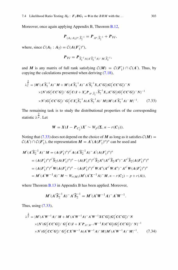
7.4 Likelihood Ratio Testing H0 : F 1BG1 = 0 in the BRM with the. . . 303
Moreover, once again applying Appendix B, Theorem B.12,
P(A1:A2)o,S−1
2= P
Ao,S−12
+ PW ,
where, since C(A1 : A2) = C(A(F ′1)
o),
PW = PS−1
2 A(A′S−12 A)−M,S−1
2,
and M is any matrix of full rank satisfying C(M) = C(F ′1) ∩ C(A′). Thus, by
copying the calculations presented when deriving (7.18),
λ
2no = |M ′(A′
S−12 A)−M + M ′(A′
S−12 A)−A′
S−12 XoC
′Go2(G
o′2 CC′Go
2)−N
×{N ′(Go′2 CC′Go
2)−Go′
2 C(I + X′oP Ao,S−1
2
S−12 Xo)C
′Go2(G
o′2 CC′Go
2)−N}−1
×N ′(Go′2 CC ′Go
2)−Go′
2 CX′oS
−12 A(A′
S−12 A)−M ||M ′(A′
S−12 A)−M|−1. (7.33)
The remaining task is to study the distributional properties of the corresponding
statistic λ2n . Let
W = X(I − PC ′2)X′ ∼ Wp(�, n − r(C2)).
Noting that (7.33) does not depend on the choice of M as long as it satisfies C(M) =C(A′) ∩ C(F ′
1), the representation M = A′(A(F ′1)
o)o can be used and
M ′(A′S
−12 A)−M = (A(F ′
1)o)o′A(A′
S−12 A)−A′(A(F ′
1)o)o
= (A(F ′1)
o)o′S2(A(F ′
1)o)o − (A(F ′1)
o)o′S2Ao(Ao′
S2Ao)−Ao′S2(A(F ′
1)o)o
= (A(F ′1)
o)o′W (A(F ′
1)o)o − (A(F ′1)
o)o′WAo(Ao′
WAo)−Ao′W (A(F ′
1)o)o
= M ′(A′W−1A)−M ∼ Wr(M)(M′(A′�−1A)−M, n − r(C2) − p + r(A)),
where Theorem B.13 in Appendix B has been applied. Moreover,
M ′(A′S
−12 A)−A′
S−12 = M ′(A′W−1A)−A′W−1.
Thus, using (7.33),
λ2n = |M ′(A′W−1A)−M + M ′(A′W−1A)−A′W−1XC ′Go
2(Go′2 CC ′Go
2)−N
×{N ′(Go′2 CC ′Go
2)−Go′
2 C(I + X′P Ao,W−1W−1X)C ′Go2(G
o′2 CC′Go
2)−N}−1
×N ′(Go′2 CC ′Go
2)−Go′
2 CX′W−1A(A′W−1A)−M ||M ′(A′W−1A)−M|−1. (7.34)

304 7 Testing Hypotheses
Since XC′Go2 is independent of W , the expression in (7.34) has the same form
as (7.18) and it can immediately be stated that λ2/n follows the distribution of
|V + U ||V | , (7.35)
where V and U are independent, V ∼ Wr(M)(I , n − r(C2) − p + r(A)) and underH0, U ∼ Wr(M)(I , r(N)). Hence, the next two theorems can be stated and they aresimilar to Theorems 7.2 and 7.3.
Theorem 7.4 For the BRM presented in Definition 2.1 with the restrictionsF 2BG2 = 0, the null hypothesis H0: F 1BG1 = 0, F 2BG2 = 0, whereC(F ′
1) ⊆ C(F ′2), is tested against H1: F 2BG2 = 0. Let λo be the observed value
of λ, given in (7.32), and let
to = 2n(f − 1
2 (po − m + 1)) ln λo,
where f = n − r(Go′2 C) − p + r(A), po = dim{C(F ′
1) ∩ C(A′)} and m =dim{C(Go′
2 C) ∩ C(Go′2 G1)}. The likelihood ratio test, approximately at significance
level α, rejects the hypothesis if to satisfies
P {χ2pom
≥ to} + c1(1 − c1)(P {χ2pom+4 ≥ to} − P {χ2
pom≥ to})
+ c2(P {χ2pom+8 ≥ to} − P {χ2
pom≥ to}) ≤ α,
where c1 and c2 are defined in Theorem 7.2. ��Theorem 7.5 The model and hypothesis are the same as those in Theorem 7.4.
Let λo be given in (7.32) with a corresponding λ and put Upo,m,f = λ− 2n , where
po = dim{C(F ′1)∩C(A′)}, f = n− r(Go′
2 C)−p+ r(A) and m = dim{C(Go′2 C)∩
C(Go′2 G1)}. Then
(i) if po = 2, T21 = (f−1)m
(1 − U1/22,m,f )/U
1/22,m,f ∼ F2m,2(f−1);
(ii) if po = 1, T22 = fm
(1 − U1,m,f )/U1,m,f ∼ Fm,f .��
Moreover, as with (7.20), the final result presented in (7.35) was obtained byconditioning on Ao′
X. Correspondingly to (7.22) and (7.23), which were usedin (7.26) and (7.27), the following projections were utilized:
P = P 1(I − PC ′2) = I − P C ′
2− (I − P C ′
2)X′Ao(Ao′
WAo)−Ao′X(I − PC ′
2),
P 1 = I − (I − P C ′2)X′Ao(Ao′
WAo)−Ao′X.
Via these projections, dispersion matrices can be defined and random propertiesof the presented test statistic stem from the obtained dispersion matrices. The

7.4 Likelihood Ratio Testing H0 : F 1BG1 = 0 in the BRM with the. . . 305
(a) (b)
Fig. 7.5 In (a), the dotted area corresponds to H0: F 1BG1 = 0 in the BRM with the restrictionsF 2BG2 = 0, where C(F ′
1) ⊆ C(F ′2). In (b), those areas are given which, after conditioning with
respect to Ao′X, contribute to the likelihood ratio test. Furthermore, W1 = C•(A(F ′
2)o), W2 =
C•(A(F ′1)
o) ∩ C•(A(F ′2)
o)⊥, W3 = C•(A) ∩ C•(A(F ′1)
o)⊥, W4 = C•(A)⊥, V1 = C(C ′(G1 :G2)
o), V2 = C(C ′Go2) ∩ C(C ′(G1 : G2)
o)⊥, V3 = C(C′) ∩ C(C ′Go2)
⊥, V4 = C(C ′)⊥, ˜V2 =C(P
P1C′Go2(Go′
2 CC′Go2)−N
), C(N) = C(Go′2 C)∩C(Go′
2 G1) and ˜V3 +˜V4 = C(P C′2)⊥. The dispersion
matrices D31 and D13+22 are defined in (7.37) and (7.36), respectively
dispersion matrices of interest are
D13+22 = M ′(A′W−1A)−M = M ′(A′�−1A)−A′�−1XPX′�−1A(A′�−1A)−M,
(7.36)
D31 = M ′(A′�−1A)−A′�−1XPP1C′Go
2(Go′2 CC′Go
2)−NX′�−1A(A′�−1A)−M . (7.37)
Therefore,
λ2n = |D13+22 + D31|
|D13+22| . (7.38)
The likelihood ratio test, the dispersion matrices and the spaces which are involvedin building up the test are illustrated in Fig. 7.5. It is recommended that one shouldcompare Fig. 7.5 with Fig. 7.4 in order to understand the similarities and differencesbetween deriving the tests in Sect. 7.3 and deriving those in Sect. 7.4.
In the above derivation, the likelihood ratio test for testing H0 : F 1BG1 = 0 wasderived when F 2BG2 = 0 and C(F ′
1) ⊆ C(F ′2) held. However, it follows from the
derivation of the test that the same test statistic is obtained when C(F ′1) = C(F ′
2),which in fact leads to a case where the result of the test is often easier to interpretthan when C(F ′
1) ⊆ C(F ′2) occurs.
Example 7.5 In this example the same data as those in Example 7.3 are used. Thematrices which are considered are the following:
F 1 = (0 : 0 : 0 : 0 : 1), G1 = (1 : −1 : 0)′, F 2 =(
0 0 0 1 0
0 0 0 0 1
)
, G2 = (0 : 0 : 1)′.

306 7 Testing Hypotheses
For the parameters selected by F 1, the matrix G1 is used to identify that thefirst and second groups share the same parameter. With the given matrices, thelikelihood ratio λo for testing H0: F 1BG1 = 0 equals λ
2/45o = 1.06. Moreover,
po = dim{C(F ′1) ∩ C(A′)} = 1, m = dim{C(Go′
2 C) ∩ C(Go′2 G1)} = 1 and
f = n− r(Go′2 C)−p + r(A) = 45 − 2 − 10 + 5 = 38. Since po = 1, Theorem 7.5
(ii) can be used, U1,1,38 = λ−2/45o = 0.94 and
T22o = 38(1 − U1,1,38)/U1,1,38 = 2.4 < F0.05(1, 38) = 4.1.
Hence, H0 cannot be rejected at significance level 0.05. ��
7.5 Likelihood Ratio Testing H0 : F 2BG2 = 0 in the BRM
with the Restrictions F 1BG1 = 0, C(F ′1) ⊆ C(F ′
2) andC(G2) ⊆ C(G1)
In the previous section, when testing H0 : F 1BG1 = 0 in the BRM with therestrictions F 2BG2 = 0 and C(F ′
1) ⊆ C(F ′2), the EBRM3
B was utilized. Nowthe following testing problem in the BRM with the restrictions F 1BG1 = 0 isconsidered:
H0 : F 2BG2 = 0, F 1BG1 = 0, versus H1 : F 1BG1 = 0, (7.39)
where C(F ′1) ⊆ C(F ′
2) and C(G2) ⊆ C(G1). One reason for discussing this testingproblem is to present an alternative approach to the one given in the previous section.Without any loss of generality, it can be shown that it is appropriate to assumeC(G2) = C(G1) instead of C(G2) ⊆ C(G1), which, however, will not take place.Moreover, assume that C(G2) ⊆ C(G1) does not hold, i.e. the same assumptionsas in Sect. 7.4 hold. If one only focuses on H0, it follows from the assumptionF 2BG2 = 0 that F 1BG2 = 0 also holds. Hence, under H0, F 1BG1 = 0 isidentical to F 1B(G1 : G2) = 0 and, of course, C(G1) ⊆ C(G1 : G2). Thus, therestrictions on the parameter space of B under H0 are the same in Sects. 7.4 and7.5.
Example 7.6 To illustrate the test and model assumptions of this section, we usethree groups of individuals with different mean structures. Let E[X] = ABC withF 1BG1 = 0 and under H0: F 2BG2 = 0, where
A =
⎛
⎜
⎜
⎜
⎜
⎝
1 t1 t21
1 t2 t22
......
...
1 tp t2p
⎞
⎟
⎟
⎟
⎟
⎠
, C = (1′n1
⊗ (1 : 0 : 0)′ : 1′n2
⊗ (0 : 1 : 0)′ : 1′n3
⊗ (0 : 0 : 1)′),

7.5 Likelihood Ratio Testing H0 : F 2BG2 = 0 in the BRM with the. . . 307
F 1 = (0 : 0 : 1), G1 =⎛
⎜
⎝
0 0
0 1
1 0
⎞
⎟
⎠ , F 2 =(
0 0 1
0 1 0
)
, G2 = (0 : 1 : 0)′.
Hence, C(F ′1) ⊆ C(F ′
2) and C(G2) ⊆ C(G1). The “growth” for one of the groups ismodelled with a second-order polynomial; i.e. one of the groups has a quadraticgrowth and the two other groups follow a linear growth. Moreover, it is testedwhether one of the two groups with a linear growth has a constant mean. Thus,under H0, one group has a constant mean, one group follows a linear mean modeland one group follows a quadratic mean model.
It is clear that under H0, the mean has a nested structure in the same way as ithas with the EBRM3
B or EBRM3W . Under the alternative hypothesis, the treatment
groups follow either a linear or a quadratic mean model. Let B = (bij ), and thenalternatively to the matrix formulation of the restrictions F iBGi = 0, i = 1, 2, thehypothesis can be written as H0: b32 = b33 = b22 = 0. ��The general solution to the system of equations F 1BG1 = 0, F 2BG2 = 0is presented in Appendix B, Theorem B.10 (iii). With the additional subspaceconditions, the results imply the following mean structure:
E[X] = A�1Go′1 C + A(F ′
1)o�2(G2 : Go
1)o′C + A(F ′
2)o�3G
′2C.
This means that under H 0, since C(A(F ′2)
o) ⊆ C(A(F ′1)
o) ⊆ C(A), the meanmodel yields an EBRM3
W . Hence, Theorem 3.3 provides the MLE for �, i.e.
n�H0 = S3 + P ′Ao
1,S−13
XP C ′1X′P
Ao1,S−1
3,
S3 = S2 + P ′Ao
2,S−12
XP 2X′P
Ao2,S−1
2,
S2 = S1 + P ′Ao
3,S−11
XP 3X′P
Ao3,S
−11
,
where P 2 and P 3 are orthogonal projectors on C(C′1)
⊥ ∩ C(C′1 : C′
2) and C(C′1 :
C′2)
⊥ ∩ C(C′), respectively, A1 = A, A2 = A(F ′1)
o, A3 = A(F ′2)
o, S1 = X(I −P C ′)X′, C1 = Go′
1 C, C2 = (G2 : Go1)
o′C and C3 = G′
2C.For the alternative hypothesis there is only the restriction F 1BG1 = 0 on the
mean parameter space and in this case the mean of the model may be written asfollows:
E[X] = A�1Go′1 C + A(F ′
1)o�2G
′1C. (7.40)

308 7 Testing Hypotheses
Since C(A(F ′1)
o) ⊆ C(A), it follows that in this case there is an EBRM2W which
has to be considered. Thus, from Theorem 3.3,
n�H1 = S˜
2 + P ′Ao
1,S˜
−12
XP C ′1X′P
Ao1,S˜
−12
,
S˜
2 = S1 + P ′Ao
2,S−11
XP 4X′P
Ao2,S
−11
, (7.41)
where P 4 is the orthogonal projector on C(C′) ∩ C(C′1)
⊥, A1 = A, A2 = A(F ′1)
o,
C1 = Go′1 C, C2 = G′
1C and S1 = X(I − PC ′)X′. This implies that under H0 andH1, the matrices A1, A2, C1 and S1 are the same. Note also that the parameter �1in (7.40) is not affected by the hypothesis.
Using the same type of calculations as in the previous sections, it can be shownthat the likelihood ratio statistic is equivalent to
λ
2no = |�H0 |
|�H1 |= |S3||Ao′
S3Ao|−1|Ao′
XoX′oA
o||S˜
2||Ao′S˜
2Ao|−1|Ao′
XoX′oA
o| . (7.42)
Since P 4 = P 2 + P 3 it follows that Ao′S3A
o = Ao′S˜
2Ao and Ao′
2S3A
o2 =
Ao′2S˜
2Ao2. Moreover, expanding |S3| and |S
˜
2| yields
λ
2no = |S2||Ao′
2S2A
o2|−1|Ao′
2 (S1 + XoP 3X′o + XoP 2X
′o)A
o2|
|S1||Ao′2 S1A
o2|−1|Ao′
2 (S1 + XoP 4X′o)A
o2|
= |S2||Ao′2S2A
o2|−1
|S1||Ao′2 S1A
o2|−1
, (7.43)
which has the same form as (7.14); i.e. replacing A in (7.14) by A2 = A(F ′1)
o andreplacing A1 = A(F ′)o in (7.14) by A3 = A(F ′
2)o lead to (7.14) being identical
to (7.43), where in particular
S2 = S1 + P ′Ao
3,S−11
X(PC ′1− P C ′
2)X′P
Ao3,S
−11
.
Thus, if one replaces observations by random variables,
λ2n = |A′
2S−11 A2|
|A′2S
−12 A2|
. (7.44)

7.5 Likelihood Ratio Testing H0 : F 2BG2 = 0 in the BRM with the. . . 309
Indeed, the above observations immediately show the possibility of using (7.18) (seealso (7.15)), which implies that the likelihood ratio test statistic is given by
λ2n = |M ′(A′
2S−11 A2)
−M + M ′(A′2S
−11 A2)
−A′2S
−11 XC′(CC′)−N
×{N ′(CC ′)−C(I + X′PAo
2,S−11
S−11 X)C ′(CC′)−N}−1
×N ′(CC ′)−CX′S−11 A2(A
′2S
−11 A2)
−M||M ′(A′2S
−11 A2)
−M|−1, (7.45)
where S1 = X(I − P C ′)X′, and M and N are any matrices of full rank satisfying
C(M) = C((F ′1)
o′A′(A(F ′
2)o)o),
C(N) = C(C) ∩ C(G2).
Put
P 1 = I − (I − P C′ )X′Ao2(A
o′2 S1A
o2)
−Ao′2 X, (7.46)
P = P 1(I − P C′ ) = I − PC′ − (I − P C′ )X′Ao2(A
o′2 S1A
o2)
−Ao′2 X(I − PC′ ). (7.47)
Then it can be shown that λ2n has the same distribution as (see also Theorem 7.4
and (7.28))
|V + U ||V | , (7.48)
where V ∼ Wr(M)(I , r(P )) and U ∼ Wr(M)(I , r(P 1C′(CC′)−N)) with r(P ) =
n − r(C) − p + r(A′ : F ′1) − r(F 1) and r(P 1C
′(CC′)−N) = r(N). Hence, thenext two theorems have been verified.
Theorem 7.6 For the BRM presented in Definition 2.1 with the restrictionsF 2BG2 = 0, the null hypothesis H0: F 1BG1 = 0, F 2BG2 = 0 is tested againstH1: F 1BG1 = 0; i.e. all elements in F 2BG2 differ from 0, with C(F ′
1) ⊆ C(F ′2)
and C(G2) ⊆ C(G1). Let λo be the observed value of λ, given in (7.44), and let
to = 2n(f − 1
2 (po − m + 1)) ln λo,
where f = n− r(C)−p+ r(A′ : F ′1)− r(F 1), po = dim{C((F ′
1)o′A′(A(F ′
2)o)o)}
and m = dim{C(G2) ∩ C(C)}. The likelihood ratio test, approximately at signifi-cance level α, rejects the hypothesis if to satisfies
P {χ2pom
≥ to} + c1(1 − c1)(P {χ2pom+4 ≥ to} − P {χ2
pom≥ to})
+ c2(P {χ2pom+8 ≥ to} − P {χ2
pom≥ to}) ≤ α,
where c1 and c2 are defined in Theorem 7.2. ��

310 7 Testing Hypotheses
Theorem 7.7 The model and hypothesis given below are the same as those in
Theorem 7.6. Let λ be given in (7.44) and put Upo,m,f = λ− 2n , where po =
dim{C((F ′1)
o′A′(A(F ′
2)o)o)}, f = n − r(C) − p + r(A′ : F ′
1) − r(F 1) andm = dim{C(G2) ∩ C(C)}. Then(i) if po = 2, T23 = (f−1)
m(1 − U
1/22,m,f )/U
1/22,m,f ∼ F2m,2(f−1);
(ii) if po = 1, T24 = fm
(1 − U1,m,f )/U1,m,f ∼ Fm,f .��
As in the previous sections, we can try to understand what we are testing and howwe are testing the hypothesis H0: F 2BG2 = 0 when applying the likelihood ratiostatistic, i.e. try to find some expressions which correspond to (7.36) and (7.37).Define the dispersion matrices
D12 = M ′(A′2S−1
1 A2)−M = M ′(A′2�−1A2)−A′
2�−1XPX′�−1A2(A′2�−1A2)−M, (7.49)
D22 = M ′(A′2�−1A2)−A′
2�−1XPP1C′(CC′)−NX′�−1A2(A′2�−1A2)−M, (7.50)
where P and P 1 are defined in (7.47) and (7.46). Then applying these definitionsto (7.45) yields after some calculations, similar to those used for handling (7.34)and (7.18),
λ2n = |D12 + D22|
|D12| ,
which in fact also explains (7.48). The dispersion matrices are illustrated in Fig. 7.6.The figure should be compared to Fig. 7.5, and the difference between the figuresshows how the different hypotheses (restrictions) act on the mean space.
Moreover, it is interesting to note, concerning the way in which the test isderived, that one could consider the calculations as using a conditional approach,i.e. conditioning with respect to Ao′
2 X. Note that at the end of the derivation, the
distribution of the test statistic is indeed independent of Ao′2 X. This idea will also
be utilized later in Sect. 7.7.
Example 7.7 In this example, the data which were generated in Example 7.3 areconsidered again. However, now the additional condition C(G2) ⊆ C(G1) isimposed. The matrices which define the restrictions on the parameter space are
F 1 = (0 : 0 : 0 : 0 : 1), G1 =⎛
⎝
0 00 11 0
⎞
⎠ , F 2 =(
0 0 0 0 10 0 0 1 0
)
, G2 = (0 : 1 : 0)′,

7.5 Likelihood Ratio Testing H0 : F 2BG2 = 0 in the BRM with the. . . 311
(a) (b)
Fig. 7.6 In (a), the dotted area corresponds to H0: F 2BG2 = 0 in the BRM with the restrictionsF 1BG1 = 0, where C(F ′
1) ⊆ C(F ′2) and C(G′
2) ⊆ C(G′1). In (b), those areas are given, which
after conditioning with respect to Ao′2 X, contribute to the likelihood ratio test. Furthermore, W1 =
C•(A(F ′2)
o), W2 = C•(A(F ′1)
o) ∩ C•(A(F ′2)
o)⊥, W3 = C•(A) ∩ C•(A(F ′1)
o)⊥, W4 = C•(A)⊥,V1 = C(C ′Go
1), V2 = C(C′Go2) ∩ C(C ′Go
1)⊥, V3 = C(C ′) ∩ C(C′Go
2)⊥, V4 = C(C ′)⊥, ˜V3 =
C(P P1C′(CC′)−N), C(N ) = C(Go′2 C) ∩ C(Go′
2 G1) and ˜V4 = C(P ), where P 1 and P are definedin (7.46) and (7.47), respectively. Moreover, the dispersion matrices D22 and D12 are definedin (7.50) and (7.49), respectively
which satisfy C(F ′1) ⊆ C(F 2) and C(G2) ⊆ C(G1). The restrictions under H0:
F 1BG1 = 0, F 2BG2 = 0, if B = (bij ), yield b42 = 0, b52 = 0 and b53 = 0. In
this case, the test statistic given by (7.42) takes the value λ2/45o = 1.9 and, hence,
Upo,m,f = 0.51. Moreover, po = 1, m = 1 and f = 36. Thus, from Theorem 7.7(ii),
T24o = 36(1 − U1,1,36)/U1,1,36 = 34.1 > F0.05(1, 36) = 4.1
and the hypothesis H0: F 2BG2 = 0 is rejected.Instead of G1, the subvector ˜G1 = (0 : 0 : 1)′ can be used in order to avoid any
overlap between F 1BG1 = 0 and F 2BG2 = 0; for instance in the present exampleF 1BG2 = 0 appears in both F 1BG1 = 0 and F 2BG2 = 0. In this case, of course,we are back in Sect. 7.4.
If instead of G2 = (0 : 1 : 0)′, the between-individuals matrix G2 = (0 : 0 : 1)′is used, we are closer to the model which generated the data in Example 7.3 andobtain
T24o = 36(1 − U1,1,36)/U1,1,36 = 1.6 < F0.05(1, 36) = 4.1,
and this time H0 is not rejected. ��

312 7 Testing Hypotheses
7.6 Likelihood Ratio Testing H0 : F iBGi = 0, i = 1, 2,Against B Unrestricted in the BRM with C(F ′
1) ⊆ C(F ′2)
Now we consider a more challenging testing situation than the situations discussedin the previous sections, i.e.
H0 : F iBGi = 0, i = 1, 2, versus B unrestricted, (7.51)
where C(F ′1) ⊆ C(F ′
2). In Fig. 7.7a, b, the spaces which correspond to thehypotheses tested in Sects. 7.3 and 7.4 are illustrated. In this section the structurepresented in Fig. 7.7c is discussed. It is immediately seen that the hypothesisgenerates a restriction on the parameter space which has a different form comparedwith the restrictions in the previous sections, and therefore it also appears that thetesting problem differs from the problems in the previous sections. Unfortunately,the spaces connected to the indicated area of Fig. 7.7c will generate a likelihood ratiowhich is more difficult to handle as precisely as the ratios in the earlier sections werehandled. On the other hand, the hypothesis treated in this section, i.e. (7.51), is ina sense the most natural extension of H0 : FBG = 0, which was discussed, inSect. 7.3 in particular.
From Theorems 3.1 and 3.2 (see also (7.31)), it follows that the likelihood ratiofor testing (7.51) is equivalent to
λ
2no = |�H0 |
|�H1 |= |S3 + Q
′3Q
′2Q
′1XoP C ′
3X′
oQ1
Q2Q3|
|S1 + P ′Ao,S−1
1XoP C ′X′
oP Ao,S−11
| , (7.52)
(a) (b) (c)
Fig. 7.7 In (a), the dotted area corresponds to H0: F 2BG2 = 0 in the BRM . In (b), the area isshown for testing H0: F 1BG1 = 0 in the BRM , given F 2BG2 = 0, where C(F ′
1) ⊆ C(F ′2), and
in (c), the area is shown for testing H0: F iBGi = 0, i = 1, 2, in the BRM , where C(F ′1) ⊆ C(F ′
2)
holds. Furthermore, W1 = C•(A(F ′2)
o), W2 = C•(A(F ′1)
o) ∩ C•(A(F ′2)
o)⊥, W3 = C•(A) ∩C•(A(F ′
1)o)⊥, W4 = C•(A)⊥, V1 = C(C ′(G1 : G2)
o), V2 = C(C ′Go2) ∩ C(C′(G1 : G2)
o)⊥,V3 = C(C′) ∩ C(C ′Go
2)⊥ and V4 = C(C ′)⊥

7.6 Likelihood Ratio Testing H0 : F iBGi = 0, i = 1, 2, Against B . . . 313
where the notation follows that of Sect. 7.4. However, an interesting factorization ofλo can take place, namely
λo = λ1oλ2o,
where
λ
2n1o =
|S2 + P ′Ao,S−1
2XoPC ′
2X′
oP Ao,S−12
||S1 + P ′
Ao,S−11
XoP C ′X′oP Ao,S−1
1| , (7.53)
λ
2n2o =
|S3 + P ′Ao,S−1
3XoPC ′
3X′
oP Ao,S−13
||S2 + P ′
Ao,S−12
XoPC ′2X′
oP Ao,S−12
| . (7.54)
Then it is noted that, correspondingly to λ1o, given in (7.53), λ1 is the test statisticfor testing a BRM with respect to H0: F 2BG2 = 0 against B unrestricted, whichwas presented in Sect. 7.3, i.e. Theorems 7.2 and 7.3. Moreover, correspondingly toλ2o, given in (7.54), λ2 is the statistic used for testing, within a BRM framework,H0: F 1BG1 = 0, given that F 2BG2 = 0 holds, which was treated in Sect. 7.4,i.e. Theorems 7.4 and 7.5.
Expressing the statistics with the help of dispersion matrices, it follows fromSect. 7.3 and (7.28) that
λ
2n1 = |A′S−1
1 A||A′
S−12 A|
= |D12 + D21||D12| , (7.55)
where
D12 ∼ Wr(M1)(M′1(A
′�−1A)−M1, r(P )),
r(P ) = n − r(C) − p + r(A),
D21 ∼ Wr(M1)(M′1(A
′�−1A)−M1, r(N1)),
with M1 and N1 satisfying
C(M1) = C(F ′2) ∩ C(A′), C(N1) = C(G2) ∩ C(C).
Section 7.4 and (7.38) yield that λ2 can be expressed as follows:
λ
2n2 = |A′S−1
2 A||A′
S−13 A|
= |D13+22 + D31||D13+22| , (7.56)

314 7 Testing Hypotheses
where
D13+22 ∼ Wr(M2)(M′2(A
′�−1A)−M2, r(P )),
r(P ) = n − r(C2) − p + r(A),
D31 ∼ Wr(M2)(M′2(A
′�−1A)−M2, r(N2)),
with M2 and N2 satisfying
C(M2) = C(F ′1) ∩ C(A′), C(N2) = C(Go′
2 C) ∩ C(Go′2 G1).
However, it can be shown that λ1 and λ2 are not independently distributed, whichmeans that the interpretation of the statistics becomes complicated. Unfortunately,the joint distribution of λ1 and λ2 is not easy to obtain. In order to find anapproximate upper bound of the p-value for testing (7.51) via (7.52), a Bonferronicorrection may take place. In general, the Bonferroni approach also overcomesthe difficulty associated with any dependence among the tests and is definitelysuitable when only a few tests are to be considered. For example, in our case thisapproach can be used since there are only two tests to be performed. Moreover, itis interesting to discover that the factorization of the likelihood ratio test statistichas a natural hierarchy; i.e. one should first apply λ1 and thereafter λ2, given thatH0: F 2BG2 = 0 has not been rejected. If the test is rejected in the first step, thenthe test described in (7.51) should, of course, also be rejected. Hence, a testingstrategy has been derived which is similar, for example, to classical profile analysisin multivariate analysis. Since the tests based on λ1 and λ2 are not independent, itis quite natural to use equal rejection probabilities, although it is not necessary tocarry out the overall test in this way.
Theorem 7.8 For the BRM presented in Definition 2.1, let, as in (7.51), the nullhypothesis H0: F iBGi = 0, i = 1, 2, where C(F ′
1) ⊆ C(F ′2) holds, be tested
against the alternative hypothesis H1: B is unrestricted. Let λ1o and λ2o be theobserved values of λ1 and λ2, defined by (7.53) and (7.54), respectively. Moreover,let
t1o = 2n(f1 − 1
2 (p1o − m1 + 1)) ln λ1o,
t2o = 2n(f2 − 1
2 (p2o − m2 + 1)) ln λ2o,
where
f1 = n − r(C) − p + r(A), f2 = n − r(C2) − p + r(A),
p1o = dim{C(F ′2) ∩ C(A′)}, p2o = dim{C(F ′
1) ∩ C(A′)},m1 = dim{C(G2) ∩ C(C)}, m2 = dim{C(Go′
2 C) ∩ C(Go′2 G1)}.

7.6 Likelihood Ratio Testing H0 : F iBGi = 0, i = 1, 2, Against B . . . 315
The likelihood ratio test for this hypothesis, approximately on level α, rejects thehypothesis if
P {χ2p1om1
≥ t1o} + c11(1 − c11)(P {χ2p1om1+4 ≥ t1o} − P {χ2
p1om1≥ t1o})
+ c12(P {χ2p1om1+8 ≥ t1o} − P {χ2
p1om1≥ t1o}) ≤ α1,
or
P {χ2p2om2
≥ t2o} + c21(1 − c21)(P {χ2p2om2+4 ≥ t2o} − P {χ2
p2om2≥ t2o})
+ c22(P {χ2p2om2+8 ≥ t2o} − P {χ2
p2om2≥ t2o}) ≤ α2,
where c11 and c12 correspond to c1 and c2 in Theorem 7.2, with p1o, m1 and f1inserted, c21 and c22 correspond to c1 and c2 in the same theorem, with p2o, m2 andf2 inserted, and α1 + α2 = α. ��In Theorem 7.8 it was suggested to use α1 + α2 = α, where α is the prespecifiedsignificance level. Since λ1 and λ2 are not independently distributed it is difficult tofind α1 and α2 so that the Type I error equals exactly α. Therefore it is reasonable toapply the Bonferroni approach when choosing α1 and α2. However, note that underindependence of the two hypotheses we can use the relation
(1 − α) = (1 − α1)(1 − α2) = 1 − α1 − α2 + α1α2,
i.e. the overall hypothesis is not rejected if the hypothesis connected to λ1 and thehypothesis connected to λ2 are not rejected. Since α1α2 will be small it makessense to also under independence use α1 + α2 = α. An exception would be ifthe distribution of λ1λ2 could be found.
Example 7.8 Here, once again, the melatonin data generated in Example 7.3 areconsidered. Now, for the BRM , H0: F iBGi = 0, i = 1, 2, against B unrestrictedis tested with the following matrices:
F 1 = (0 : 0 : 0 : 0 : 1), G1 = (0 : 0 : 1)′, F 2 =(
0 0 0 0 1
0 0 0 1 0
)
, G2 = (0 : 1 : 0)′,
and in comparison with Example 7.3, G1 and G2 are interchanged, which meansthat the hypothesis which is tested in this example differs from the true model fromwhich data have been generated. Moreover, alternatively, it can be stated that forB = (bij ), the restrictions equal b53 = b52 = b42 = 0. From the derivation, itfollows that λ1 is a test statistic for testing b52 = b42 = 0, and λ2 tests b53 = 0given that b52 = b42 = 0.

316 7 Testing Hypotheses
To calculate λ1o, the matrices S1 and S2 are needed, which equal S1 = Xo(I −P C ′)X′
o and
S2 = S1 + P ′Ao
1,S−11
Xo(P C ′1− P C ′
2)X′
oP Ao1,S−1
1,
where A1 = A(F ′2)
o, C1 = C and C2 = Go′2 C. Moreover, (F ′
2)o = (I 3 : 0) and
Go′2 =
(
1 0 00 0 1
)
.
Concerning the second test, to calculate λ2o, additionally the following definition isneeded:
S3 = S2 + P ′(A1:A2)o,S−1
2Xo(P C ′
2− P C ′
3)X′
oP (A1:A2)o,S−12
,
where A2 = A(F ′1 : (F ′
2)o)o = A(0 : 0 : 0 : 1 : 0)′, C1 = C, and C3 = (G1 :
G2)o′C = (1 : 0 : 0)C.
The test connected with λ1, H0: F 2BG2 = 0 versus B unrestricted, is rejectedsince U2,1,37 = λ
−2/452o = 1.95−1 = 0.51, and from Theorem 7.3 (i)
T11o = 36(1 − U1/22,1,37)/U
1/22,1,37 = 14.3 > F0.05(2, 72) = 4.1.
Thus, the overall hypothesis H0: F iBGi = 0, i = 1, 2, is rejected.Parenthetically it is noted that the test connected with λ2, H0: F 1BG1 = 0 given
F 2BG2 = 0, is not rejected since U1,1,38 = λ−2/452o = 1.03−1 = 0.97, and from
Theorem 7.5 (ii)
T22o = 38(1 − U1,1,38)/U1,1,38 = 1.2 < F0.05(1, 38) = 3.1.
Next we investigate what happens if
F 1 = (0 : 0 : 0 : 0 : 1), G1 = (0 : 0 : 1)′, F 2 =
⎛
⎜
⎜
⎝
0 0 0 0 10 0 0 1 00 0 1 0 00 1 0 0 0
⎞
⎟
⎟
⎠
, G2 = (1 : 0 : 0)′

7.7 Likelihood Ratio Testing H0 : F iBGi = 0, i = 1, 2, Against B . . . 317
are used, which is a rather extreme suggestion in relation to how the data have beengenerated. Thus, C1 = C, C2 = Go′
2 C = (0 : I 2)C, C3 = (G1 : G2)o′C = (0 : 1 :
0)C,
A1 = A(F ′2)
o = A
⎛
⎜
⎜
⎜
⎜
⎜
⎝
10000
⎞
⎟
⎟
⎟
⎟
⎟
⎠
, A2 = A(F ′1 : (F ′
2)o)o = A
⎛
⎜
⎜
⎜
⎜
⎜
⎝
0 0 01 0 00 1 00 0 10 0 0
⎞
⎟
⎟
⎟
⎟
⎟
⎠
,
and A3 = AF ′1. When testing F 2BG2 = 0, since p1o = 4, Theorem 7.8 is
suggested to be used. In this case, λ2/451o = 1.34, t1o = 10.2 and applying the
theorem yields P {χ24 ≥ t1o} = 0.04 < 0.05 and thus H0 is rejected. Note that
the same test was performed in Sect. 7.3, in Example 7.3. Moreover, λ2/452o = 1.0
and then the corresponding H0 is not rejected, which, however, is extraneous tothe conclusions concerning the rejection of the hypothesis about the double bilinearrestrictions. It is worth noting that as long as C(F ′
1) ⊆ C(F ′2), the value λ1o will
not depend on the choice of F ′1 and λ2o will not depend on the choice of F ′
2. Thisobservation helps us to evaluate and break down the overall test defined throughthe double bilinear restrictions; i.e. we can, for example, marginally interpretF 1BG1 = 0. ��
7.7 Likelihood Ratio Testing H0 : F iBGi = 0, i = 1, 2,Against B Unrestricted in the BRM with C(F ′
1) ⊆ C(F ′2)
and C(G2) ⊆ C(G1)
It was seen in the previous section that a test statistic appeared which was somewhatdifferent from the test statistics of the other sections, since it “naturally” presenteda product of two test statistics instead of being only one statistic. The tests in theprevious section were, however, not independently distributed, which should betaken into account when interpreting them. The fact is, however, that the dependenceof these tests is difficult to handle in a precise manner. Now we exploit what happensif, additionally, the condition C(G2) ⊆ C(G1) is imposed on the testing problem ofthe previous section, i.e. what happens in the BRM when C(F ′
1) ⊆ C(F ′2) and
C(G2) ⊆ C(G1) hold. The hypothesis of interest is given by
H0 : F iBGi = 0, i = 1, 2, versus B unrestricted. (7.57)

318 7 Testing Hypotheses
From Sect. 7.5, recall the following matrices:
A1 = A, A2 = A(F ′1)
o, A3 = A(F ′2)
o, (7.58)
C1 = Go′1 C, C2 = (G2 : Go
1)o′C, C3 = G′
2C,
which can be used to express �H0 . Then, as in Sect. 7.5,
S3 = S2 + P ′Ao
2,S−12
XP 2X′P
Ao2,S−1
2,
S2 = S1 + P ′Ao
3,S−11
XP 3X′P
Ao3,S
−11
,
S1 = X(I − P C ′)X′,S˜
2 = S1 + P ′Ao
2,S−11
XP 4X′P
Ao2,S
−11
,
where P 2, P 3 and P 4 are orthogonal projectors on C(C′1)
⊥ ∩ C(C′1 : C′
2), C(C′1 :
C′2)
⊥ ∩ C(C′) and C(C′) ∩ C(C′1)
⊥, respectively.Utilizing the maximum likelihood estimator of � in the BRM , i.e. the unre-
stricted case, and �H0 of Sect. 7.5, it follows that the likelihood ratio test for testingH0 in (7.57) is based on
λ
2no = |�H0 |
|�H1 |=
|S3 + P ′Ao
1,S−13
XoP C ′1X′
oPAo1,S−1
3|
|S1 + P ′Ao
1,S−11
XoP C ′X′oP Ao
1,S−11
| .
In Sect. 7.6, as already mentioned, it was shown that the ratio λo could be factorized.Since, in the present section, only the condition C(G′
2) ⊆ C(G′1) has been added,
this may of course also take place here. It follows that
λo = λ1oλ2o,
where
λ
2n1o =
|S˜
2 + P ′Ao
1,S˜
−12
XoPC ′1X′
oP Ao1,S˜
−12
||S1 + P ′
Ao1,S
−11
XoP C ′X′oP Ao
1,S−11
| , (7.59)
λ
2n2o =
|S3 + P ′Ao
1,S−1
3XoPC ′
1X′
oP Ao1,S−1
3|
|S˜
2 + P ′Ao
1,S˜
−12
XoPC ′1X′
oP Ao1,S˜
−12
| , (7.60)
with the important observation that within the BRM frame, correspondinglyto (7.59) and (7.60), λ1 is a statistic for testing H0: F 1BG1 = 0 against norestrictions on B (which was presented in Sect. 7.3, Theorems 7.2 and 7.3), and λ2

7.7 Likelihood Ratio Testing H0 : F iBGi = 0, i = 1, 2, Against B . . . 319
is a statistic for testing H0: F 2BG2 = 0, C(F ′1) ⊆ C(F ′
2), C(G2) ⊆ C(G1), giventhat F 1BG1 = 0 (which was considered in Theorems 7.6 and 7.7 of Sect. 7.5).
Now we investigate the role which the condition C(G2) ⊆ C(G1) can play when
obtaining the distribution of the test statistic λ2n . Note that S
˜
2, given by (7.41),equalsS2 of Sect. 7.3 if one replaces F by F 1 and since P 4 is identical to P C ′
1−P C ′
2of Sect. 7.3. Moreover, from Sect. 7.3, it follows that λ1 can be written as follows:
λ
2n1 = |V 1 + U 1|
|V 1| ,
with
V 1 = (M ′1(A
′�−1A)−M1)−1/2M ′
1(A′�−1A)−A′�−1XPX′�−1A(A′�−1A)−
×M1(M′1(A
′�−1A)−M1)−1/2 ∼ Wr(M1)(I , n − r(C) − p + r(A)), (7.61)
U 1 = (M ′1(A
′�−1A)−M1)−1/2M ′
1(A′�−1A)−A′�−1X
×P 1C′(CC ′)−N1(N
′1(CC′)−CP ′
1P 1C′(CC′)−N1)
−N ′1(CC ′)−CP ′
1
×X′�−1A(A′�−1A)−M1(M′1(A
′�−1A)−M1)−1/2 ∼ Wr(M1)(I , r(N1)),
(7.62)
where M1 satisfies C(M1) = C(A′)∩C(F ′1), C(N1) = C(C)∩C(G1), P and P 1 are
defined in (7.22) and (7.23), respectively; V 1 and U 1 are independently distributed.Turning to λ2 and applying the results of Sect. 7.5 yield
λ
2n2 = |V 2 + U 2|
|V 2| ,
with
V 2 = (M ′2(A
′2�
−1A2)−M2)
−1/2M ′2(A
′2�
−1A2)−A′
2�−1XP 22X
′
×�−1A2(A′2�
−1A2)−M2(M
′2(A
′2�
−1A2)−M2)
−1/2 ∼ Wr(M2)(I , r(P 22)),
U2 = (M ′2(A
′2�
−1A2)−M2)
−1/2M ′2(A
′2�
−1A2)−A′
2�−1X
×P 12C′(CC ′)−N2(N
′2(CC′)−CP ′
12P 12C′(CC ′)−N2)
−N ′2(CC′)−CP ′
12
×X′�−1A2(A′2�
−1A2)−M2(M
′2(A
′2�
−1A2)−M2)
−1/2 ∼ Wr(M2)(I , r(N2)),
where M2 satisfies C(M2) = C((F ′1)
o′A′(A(F ′
2)o)o), C(N2) = C(C)∩C(G2), and
P 22 and P 12 correspond to P and P 1, defined in (7.47) and (7.46), respectively;V 2 and U2 are independently distributed.
Both λ1 and λ2 are functions of Wishart-distributed random variables. InSect. 7.6, λi , i = 1, 2, were not functions of independently distributed variables.However, with regard to λ1 and λ2 of this section is now shown that they are

320 7 Testing Hypotheses
independently distributed test statistics. Let
Y 1 = M ′1(A
′�−1A)−A′�−1X,
Y 2 = M ′2(A
′2�
−1A2)−A′
2�−1X
and note that
C[Y 1,Y 2] = I ⊗ M ′1(A
′�−1A)−A′�−1A2(A′2�
−1A2)−M2.
Since C(M1) = C(A′) ∩ C(F ′1), one can, without any loss of generality, choose M1
to equal
M1 = A′(A(F ′1)
o)o.
Thus,
M ′1(A
′�−1A)−A′�−1A2(A′2�
−1A2)−M2
= (A(F ′1)
o)o′A2(A
′2�
−1A2)−M2 = 0,
since by the definition of A2 in (7.58), it is trivially obtained that (A(F ′1)
o)o′A2 = 0.
Hence, Y 1 and Y 2 are independently distributed. Now U1 and V 1 are functionsof Y 1 and at the same time independent of Ao′
X. Moreover, U 2 and V 2 arefunctions of Y 2, as well as being independent of Ao′
2 X. Therefore, based on theseobservations, λ1 and λ2 are independently distributed.
In Fig. 7.8 the spaces which are involved in testing (7.57) are presented. Acomparison of Fig. 7.7 with Fig. 7.8 yields that the figures are very similar. Theonly difference is that the space V2 = C(C′Go
2) ∩ C(C′(G1 : G2)o)⊥ in Fig. 7.7
(a) (b) (c)
Fig. 7.8 In (a), the dotted area corresponds to H0: F 2BG2 = 0 in the BRM . In (b), the area isshown for testing H0: F 1BG1 = 0 in the BRM , given F 2BG2 = 0, where C(F ′
1) ⊆ C(F ′2), and
in (c), the area is shown for testing H0: F iBGi = 0, i = 1, 2, in the BRM , where C(F ′1) ⊆ C(F ′
2)
and C(G2) ⊆ C(G1) hold. Furthermore, W1 = C•(A(F ′2)
o), W2 = C•(A(F ′1)
o) ∩ C•(A(F ′2)
o)⊥,W3 = C•(A) ∩ C•(A(F ′
1)o)⊥, W4 = C•(A)⊥, V1 = C(C ′Go
1), V2 = C(C′Go2) ∩ C(C ′Go
1)⊥,
V3 = C(C′) ∩ C(C ′Go2)
⊥ and V4 = C(C ′)⊥

7.7 Likelihood Ratio Testing H0 : F iBGi = 0, i = 1, 2, Against B . . . 321
differs from V2 = C(C′Go2) ∩ C(C′Go
1)⊥ in Fig. 7.8. The question arises, of course,
of whether the difference is crucial, and the answer is that this difference may beimportant, but that it will not matter in many cases. However, one approach to adoptis that if there is a risk of a problem arising, then, if possible, one should try todesign the experiment so that C(G2) ⊆ C(G1) holds.
Theorem 7.9 For the BRM presented in Definition 2.1 let the null hypothesis H0:F iBGi = 0, i = 1, 2, where C(F ′
1) ⊆ C(F ′2) and C(G2) ⊆ C(G1) hold, be tested
against the alternative hypothesis H1: B is unrestricted. Let λ1o and λ2o be definedby (7.59) and (7.60), respectively. Moreover, let
t1o = 2n(f1 − 1
2 (p1o − m1 + 1)) ln λ1o,
t2o = 2n(f2 − 1
2 (p2o − m2 + 1)) ln λ2o,
where
f1 = n − r(C) − p + r(A), f2 = n − r(C′(G2 : Go1)
o) − p + r(A),
p1o = dim{C(F ′1) ∩ C(A′)}, p2o = dim{C((F ′
1)o′A′(A(F ′
2)o)o)},
m1 = dim{C(G1) ∩ C(C)}, m2 = dim{C(G2) ∩ C(C)}.
Then the likelihood ratio test for testing H0, approximately at significance level α,rejects the hypothesis if
P {χ2p1om1
≥ t1o} + c11(1 − c11)(P {χ2p1om1+4 ≥ t1o} − P {χ2
p1om1≥ t1o})
+ c12(P {χ2p1om1+8 ≥ t1o} − P {χ2
p1om1≥ t1o}) ≤ α1,
or
P {χ2p2om2
≥ t2o} + c21(1 − c21)(P {χ2p2om2+4 ≥ t2o} − P {χ2
p2om2≥ t2o})
+ c22(P {χ2p2om2+8 ≥ t2o} − P {χ2
p2om2≥ t2o}) ≤ α2,
where c11 and c12 correspond to c1 and c2 in Theorem 7.2, with p1o, m1 and f1inserted, c21 and c22 correspond to c1 and c2 in the same theorem, with p2o, m2 andf2 inserted, and α1 + α2 = α. ��Note that if pio = 1 or pio = 2, i = 1, 2, one can use Theorems 7.3 and 7.7.
Example 7.9 Reconsider the melatonin data given in Example 7.3. All the designmatrices are the same as those in Example 7.3. For the BRM , this time the nullhypothesis H0: F iBGi = 0, i = 1, 2, is tested against the alternative hypothesis

322 7 Testing Hypotheses
H1: B unrestricted, with
F 1 = (0 : 0 : 0 : 0 : 1), G′1 =
(
0 0 10 1 0
)
, F 2 =(
0 0 0 0 10 0 0 1 0
)
, G′2 = (0 : 1 : 0).
These matrices generate in B = (bij ) the restrictions b52 = b53 = b42 = 0, and λ1is the test statistic for testing b52 = b53 = 0 versus B unrestricted, while λ2 is thetest statistic for testing b42 = 0, given b52 = b53 = 0. Hence, the intention is to testH0 as in Example 7.8, but the test is carried out differently. Moreover,
(F ′1)
o =
⎛
⎜
⎜
⎜
⎜
⎜
⎝
1 0 0 00 1 0 00 0 1 00 0 0 10 0 0 0
⎞
⎟
⎟
⎟
⎟
⎟
⎠
, (F ′2)
o =
⎛
⎜
⎜
⎜
⎜
⎜
⎝
1 0 00 1 00 0 10 0 00 0 0
⎞
⎟
⎟
⎟
⎟
⎟
⎠
,
Go′1 = (1 : 0 : 0) and (G2 : Go
1)o′ = (0 : 0 : 1). Then,
A1 = A, A2 = A(F ′1)
o, A3 = A(F ′2)
o,
C1 = Go′1 C = (1 : 0 : 0)C, C2 = (G2 : Go
1)o′C = (0 : 0 : 1)C, C3 = G′
2C.
According to Theorem 7.9, the test based on λ1, given in (7.59), is not rejectedsince λ
2/451o = 1.1. However, the second test, based on λ2 which is presented
in (7.60), is rejected since λ2/452o = 1.9, which corresponds to U1,1,39 = 0.52, and
Theorem 7.7 implies that
T24o = 39(1 − U1,1,39)/U1,1,39 = 35.7 > F0.05(1, 39) = 4.1.
Thus the overall test is rejected. Now, because of the results of Example 7.8, it isreasonable to test H0: b42 = 0, since in Example 7.8, λ1o was large and in the presentexample λ2o was large. When testing H0: b42 = 0, this hypothesis can be stated inmatrix form as FBG = 0, where F = (0 : 0 : 0 : 1 : 0) and G′ = (0 : 1 : 0).Theorem 7.3 (ii) yields that H0: b42 = 0 is rejected since λ
2/45o = 1.94 and
T12o = 37(1 − U1,1,37)/U1,1,3 = 34.7 > F1,39;0.05 = 4.1.
Thus, it can be concluded that b42 = 0 is not in agreement with the observations, aswas expected based on how the data were generated in Example 7.3. ��

7.8 A “Trace Test” for the BRM , H0 : FBG = 0 Against Unrestricted B 323
7.8 A “Trace Test” for the BRM , H0 : FBG = 0 AgainstUnrestricted B
Previously, for the BRM , likelihood ratio tests for the hypotheses H0 : FBG = 0and H0 : F iBGi = 0, i = 1, 2, were considered, and the latter case was treatedunder various types of additional conditions. In this section, an alternative procedureto the likelihood ratio testing procedure is presented. The hypothesis H0 : FBG =0 is treated in this section, while H0 : F iBGi = 0, i = 1, 2, will be in focus inthe next section. In addition to a presentation of the explicit derivation of the tests, anumber of differences from the likelihood ratio tests will be pointed out. Moreover,the differences will be summarized in Sect. 7.10.
Before starting with H0 : FBG = 0, an introduction to the construction of the“trace test” statistic is presented where the hypothesis H0 : BG = 0 is discussedand several reflections on the approach are made. Consider the BRM
X = ABC + E, E ∼ Np,n(0,�, I ), (7.63)
and temporarily � is supposed to be known. In Sect. 2.4, based on linear modelstheory, the use of the estimator
ABC = P A,XP C ′
was justified, and using that, D[X] = I ⊗ � yields
D[ABC] = P C ′ ⊗ A(A′�−1A)−A′. (7.64)
It could be asserted that if one’s purpose was to make inference concerning B,it would be of interest to consider � to be a nuisance parameter. However, ithas already been established in the special case A = I that, although BC doesnot depend functionally on �, the distribution for BC does, and in particularD[BC] = P C ′ ⊗ �. Thus, strictly speaking, � cannot be considered as a nuisanceparameter. Moreover, for the interpretation of ABC, it may be fruitful to recall thatthe parameter matrix � plays two roles; i.e. it is used to mimic the variation in thedata and also is used to define the inner product. Hence, from a nuisance parameterpoint of view, the inclusion of � in P A, when estimating ABC is conceptuallynot very problematic and is to some extent independent of the variation in the data.However, one cannot circumvent the fact that the distribution connected with B
depends on �.Now, consider
S = X(I − P C ′)X′.
It is known that S is independent of XPC ′ , and S and XP C ′ , are statistics whichare jointly sufficient, with S not bearing any information about B. Thus, it is natural

324 7 Testing Hypotheses
to replace � by 1nS (or 1
n−r(C)S) in (7.64), leading to the maximum likelihood
estimator
ABC = PA,SXP C ′ . (7.65)
Moreover, similar to the conditional principle and the use of ancillarity, it isreasonable to evaluate ABC conditionally on S, i.e.
ABC|S ∼ Np,n(ABC,P A,S�P ′A,S,P C ′),
or by performing an estimation of the variation
ABC|S ∼ Np,n(ABC, 1nA(A′SA)−A′,P C ′),
where the distribution, given S = So and B, is now completely known.A competitive estimator to the maximum likelihood estimator in (7.65) is
A˜BC = PAXP C ′ ∼ Np,n(ABC,P A�P A,P C ′),
and in this case too, a conditional argument can be used to replace �, i.e.
A˜BC|S ∼ Np,n(ABC, 1nP ASP A,P C ′).
However, it is interesting to note that
P ASPA − A(A′SA)−A′ = P A(S − A(A′SA)−A′)P A
is positive semi-definite (see Appendix B, Theorem B.13). Thus, when carrying outthe conditional inference, the use of ABC has some advantages in comparison withA˜BC.
Next, as promised at the beginning of this section, the basic ideas are illustratedwith the help of a simple testing problem. For the BRM in (7.63), the hypothesisand its alternative equal
H0 : BG = 0, versus H1: B unrestricted. (7.66)
Thus, since BG = 0 is equivalent to B = �Go′, where � is an arbitrary matrix,
under H0 the BRM is defined as
X = A�Go′C + E, E ∼ Np,n(0,�, I ).
For any given �, it follows that the likelihood ratio test for H0 versus B unrestrictedis proportional to
e− 1
2 tr{�−1(Xo−ABC)()′}e
12 tr{�−1(Xo−A�Go′
C)()′}, (7.67)

7.8 A “Trace Test” for the BRM , H0 : FBG = 0 Against Unrestricted B 325
where
ABC = P A,XoP C ′, A�Go′C = P A,XoP C ′Go.
The relation in (7.67) can be written as follows:
e− 1
2 tr{�−1(S1+(I−P A,)XoP C′ X′o(I−P A,)′)}+ 1
2 tr{�−1(S2+(I−P A,)XoP C′Go X′o(I−P A,)′)}
, (7.68)
where
S1 = Xo(I − P C ′)X′o, S2 = Xo(I − P C ′Go)X′
o,
S2 − S1 = Xo(PC ′ − P C ′Go)X′o = XoPC ′(CC ′)−NX′
o,
remembering that (see Appendix B, Theorem B.12)
P C ′ − P C ′Go = P C ′(CC ′)−N,
where N is any matrix satisfying C(N) = C(G) ∩ C(C). The expression S2 − S1can be viewed as the square of the difference of two residuals.
A few manipulations in (7.68) yield that the likelihood ratio test is proportionalto
e12 tr{�−1P A,XoP C′(CC′)−NX′
oP′A, }
.
Thus, a natural test statistic for testing (7.66) is
tr{�−1P A,XP C′(CC′)−NX′P ′A,}. (7.69)
In order to acquire a deeper understanding of the test statistic in (7.69), one shouldnote that XPC ′(CC ′)−N is a projection on the between-individual subspace, and thestatistic is built up by a projection of XP C ′(CC ′)−N on the within-individuals spaceC(A), i.e.
PA,XPC ′(CC ′)−N,
and then the projection is squared. Since this takes place on the within-individualspace, the inner product has to be taken into account, meaning that
P C ′(CC ′)−NX′P ′A,�−1PA,XP C ′(CC ′)−N (7.70)

326 7 Testing Hypotheses
(a) (b)
Fig. 7.9 Consider the BRM model in (7.63). A decomposition is presented of the whole spaceaccording to the design and the restrictions BF = 0. In (a), where there are no restrictions thedecomposition consists of the subspaces C(C ′) and C(C′)⊥, as well as C(A) and C(A)⊥. In (b),with the restrictions BG = 0, V1 = C(C ′Go), V2 = C(C ′Go)⊥ ∩ C(C ′) and V3 = C(C′)⊥
should be calculated. Finally, in order to summarize the information in thisexpression, the trace is taken in (7.70), which leads to an expression which isidentical to (7.69).
For (7.69) to become applicable, � has to be replaced by an estimator. ConsiderFig. 7.9, which illustrates the fact that the hypothesis (7.66) concerns the testing of
C(C′Go)⊥ ∩ C(C′) ⊗ C(A) = C(C′(CC′)−N) ⊗ C(A),
i.e. testing whether the dimension of this space equals 0. This space is highlightedin Fig. 7.9b. However, the inner product in C(A) has to be estimated, whichmeans that a suitable estimator of � has to be found. The variation in the BRM isuncovered via projections of the observations on C(C′)⊥ ⊗W and C(C′)∩C(A)⊥,with W representing the whole within-individuals space. However, it is natural onlyto use C(C′)⊥ ⊗ W , since C(C′) ∩ C(A)⊥ depends on �; i.e. it is proposed that(I − P C ′)X should be the basis of the space where an estimator of � is obtained.Hence, as an estimator of �, when using the dispersion matrix to define the innerproduct, the quantity to use is
� = 1
nS = 1
nX(I − P C ′)X′. (7.71)
Remember that when obtaining the maximum likelihood estimators of the meanparameters in the BRM , the data were projected on the space C(C′) ∩ CS(A)⊥;i.e. the inner product was estimated using S, which is in agreement with the abovediscussion concerning the estimation of �.
Now, since PC ′(CC ′)−N is a projection on C(C′Go)⊥ ∩ C(C′), P A, is aprojection on C(A) and n−1S can be used to estimate the inner product, insteadof (7.69), a test statistic which is functionally independent of the parameters under

7.8 A “Trace Test” for the BRM , H0 : FBG = 0 Against Unrestricted B 327
H0 is given by
T3 = tr{S−1P A,SXP C′(CC′)−NX′P ′A,S}.
This statistic is called the “trace test” statistic. More precisely, it is a statistic whichbelongs to a class of “trace tests”.
Proposition 7.1 For the BRM presented in Definition 2.1, let the null hypothesisH0 : BG = 0 be tested against H1: B unrestricted. Let S be defined in (7.71) andlet N be any matrix satisfying C(N) = C(G) ∩ C(C). A test statistic is given by
T3 = tr{S−1P A,SXP C′(CC′)−NX′P ′A,S}.
The hypothesis is rejected when the observed value of T3 is large.
Moreover, it has been observed several times that S is independent ofXP C ′(CC ′)−NX′, and in the next theorem the fundamental property is stated thatthe distribution of T3, under H0, is independent of the parameters. Hence, replacing� in (7.69) by S makes sense.
Theorem 7.10 For the BRM presented in Definition 2.1, let the null hypothesisH0 : BG = 0 be tested against H1: B unrestricted. Under H0 the distribution ofthe test statistic T3, presented in Proposition 7.1, is independent of � and B.
Proof Rewrite T3 as
T3 = tr{S−1XP C′(CC′)−NX′}−tr{Ao(Ao′
SAo)−1Ao′XP C′(CC′)−NX′Ao(Ao′
SAo)−1Ao′ },
for an appropriately chosen Ao. It is noted that the first term in T3 equals
tr{S−1XP C′(CC′)−NX′} = tr{(�−1/2S�−1/2)−1�−1/2(X − A�Go′C)P C′(CC′)−N
×(X − A�Go′C)′�−1/2},
since for any �, A�Go′CC′(CC ′)−N = 0. Then under H0 the distribution
is independent of � and B . Moreover, the second term can be rewritten in thefollowing way:
tr{Ao(Ao′SAo)−1Ao′
XP C′(CC′)−NX′Ao(Ao′SAo)−1Ao′ }
= tr{Ao(Ao′�Ao)−1/2((Ao′
�Ao)−1/2Ao′SAo(Ao′
�Ao)−1/2)−1
×(Ao′�Ao)−1/2Ao′
XP C ′(CC ′)−NX′}.

328 7 Testing Hypotheses
Since the distribution of (Ao′�Ao)−1/2Ao′
X is independent of � and B, thedistribution of
(Ao′�Ao)−1/2Ao′
SAo(Ao′�Ao)−1/2
is also independent of the unknown parameters, which establishes the theorem. ��Theorem 7.11 Let T3 be defined in Proposition 7.1, and let the constants c0;n,s andci;n,s,t , i = 1, 2, 3, be given in Definition B.1 (i)–(iv), of Appendix B, Sect. B.15.Moreover, let rN = r(N), rA = r(A) and rC = r(C). Then
(i)
E[T3] = c0 + 1
n − rC − p − 1tr{�−1ABN(N ′(CC′)−N)−N ′B ′A′},
where
c0 = rN rA(n−rC−1)(n−rC−p−1)(n−rC−p+rA−1)
;
(ii) under H0
D[T3] = c1 + c2 + c3 + c4 − E[T3]2,
where E[T3] = c0, with c0 defined in statement (i), and
c1 = r2Np2c1;n−rC,p + 2rNpc2;n−rC ,p,
c2 = r2N(p − rA)2c1;n−rC,p−rA + 2rN(p − rA)c2;n−rC,p−rA,
c3 = −2r2N(p − rA)2c1;n−rC,p−rA − 4r2
N(p − rA)c2;n−rC,p−rA
− 2r2NrA(p−rA)
(n−rC−p−1)(n−rC−(p−rA)),
c4 = 2rNrA(n − rC − 1)c0;n−rC,p−rA.
Proof According to Appendix B, Theorem B.19 (iv)
E[XPC ′(CC ′)−NX′] = rN� + ABN(N ′(CC′)−N)−N ′B ′A′,
and using the independence between XP C ′(CC ′)−NX′ and S, together with Theo-rem B.26 (ii) in Appendix B, establishes statement (i).
Concerning statement (ii), since D[T3] = E[T 23 ]−E[T3]2, the expectation E[T 2
3 ]has to be determined. First it is noted that
E[T 23 ] = tr{E[(S−1P A,S)
⊗2(XP C′(CC′)−NX′)⊗2]}= tr{E[(S−1P A,S)
⊗2]E[(XP C′(CC′)−NX′)⊗2]},

7.8 A “Trace Test” for the BRM , H0 : FBG = 0 Against Unrestricted B 329
and according to Appendix B, Theorem B.19 (vii)
E[(XPC ′(CC ′)−NX′)⊗2] = r2N� ⊗ � + rN(vec�vec′� + Kp,p� ⊗ �).
Now
tr{E[(S−1P A,S)⊗2rN(vec�vec′� + Kp,p� ⊗ �)]}= 2rN tr{E[�1/2S−1A(A′S−1A)−A′S−1�S−1A(A′S−1A)−A′S−1�1/2]},
which, according to Appendix B, Theorem B.26 (iii) equals c4. The remaining taskis to derive the quantity r2
N tr{E[(S−1P A,S)⊗2� ⊗ �]}, which can be written as
r2N tr{E[(�1/2S−1�1/2 − �1/2Ao(Ao′
S−1Ao)−Ao′�1/2)⊗2]}
and is obtained via
c1 = r2N tr{E[(�1/2 ⊗ �1/2)(S−1 ⊗ S−1)(�1/2 ⊗ �1/2)]},
c2 = r2N tr{E[(�1/2Ao(Ao′
SAo)−1Ao′�1/2)⊗2]},
where Theorem B.21 (iii) in Appendix B has been used. Finally, Theorem B.24 inAppendix B determines that
c3 = −r2N tr{E[�1/2S−1�1/2 ⊗ �1/2Ao(Ao′
SAo)−1Ao′�1/2]}
−r2N tr{E[�1/2Ao(Ao′
SAo)−1Ao′�1/2 ⊗ �1/2S−1�1/2]},
and thus the proof of the theorem is complete. ��From Theorem 7.11 (i), it follows that when B �= 0, the expected value of T3 islarger than c0. Moreover, if
B1N(N ′(CC′)−N)−N ′B ′1 − B2N(N ′(CC′)−N)−N ′B ′
2
is positive semi-definite, then (see Appendix B, Theorem B.9 (ii))
tr{�−1AB1N(N ′(CC′)−N)−N ′B ′1A′} ≥ tr{�−1AB2N(N ′(CC′)−N)−N ′B ′
2A′}.
Hence, it makes sense to use T3 as a test statistic, because deviances from H0 arereflected in the test statistic.
Unfortunately, the exact distribution for T3, given by Proposition 7.1, isnot available. There are several ways to solve this problem approximatelyand it is worthwhile examining T3 more closely. First it can be noted thatS−1/2XPC ′(CC ′)−NX′S−1/2 is multivariate β-distributed of type II (see Appendix

330 7 Testing Hypotheses
A, Sect. A.9), and H = (A′S−1A)−1/2A′S−1/2 is semi-orthogonal, i.e. HH ′ = I .Thus,
T3 = tr{HS−1/2XP C′(CC′)−NX′S−1/2H ′}.
Exploiting this expression is somewhat difficult, since H and
S−1/2XP C ′(CC ′)−NX′S−1/2
are not independently distributed. Therefore, to gain a better understanding of thestatistic, a canonical version of T3 can be derived. As has been done many timesbefore, let A′ = T (I r(A) : 0)��1/2, where T is a non-singular matrix and � is anorthogonal matrix (see Appendix B, Theorem B.1 (i)). Moreover, let Y = ��−1/2X
and V = ��−1/2S�−1/2�′. Then
T3 = tr{V −1(I : 0)′((I : 0)V −1(I : 0)′)−1(I : 0)V −1YP C′(CC′)−NY ′}.
Through a spectral decomposition, it follows that
T3 =r(A)∑
i=1
λiχ2r(N);i, (7.72)
where λi are eigenvalues of
V −1(I : 0)′((I : 0)V −1(I : 0)′)−1(I : 0)V −1 =(
V 11 V 12
V 21 V 21(V 11)−1V 12
)
,
which contains already known notation. Note that in (7.72) the index i is usedto indicate that we have different chi-square variables. The distribution for T3is relatively easy to simulate, i.e. only V needs to be simulated. Then λi areobtained and, given λi , the test statistic T3 has a weighted chi-square distribution.Approximating a weighted chi-square distribution with a chi-square distribution is aclassical problem which has been studied by many authors. In the next proposition,a well-known idea is presented. However, note that λi is random, which usually isnot the case.
Proposition 7.2 For the BRM presented in Definition 2.1, let the null hypothesisH0 : BG = 0 be tested againstH1: B unrestricted. The corresponding test statisticT3 is given by Proposition 7.1. Then the hypothesis connected to T3 is rejected atapproximate significance level α if P(T3o ≥ aχ2[f ]) ≤ α, where T3o is the observedvalue of T3, [f ] denotes the integer part of either f or f + 1 and the integer part

7.8 A “Trace Test” for the BRM , H0 : FBG = 0 Against Unrestricted B 331
which is closest to f is chosen;
a = c1 + c2 + c3 + c4 − c20
2c0, f = 2c2
0
c1 + c2 + c3 + c4 − c20
,
where c0 − c4 are defined in Theorem 7.11.
Proof Below are presented a few hints explaining the choices of a and f . In (7.72)it was seen that the test statistic is a weighted sum of χ2-distributed variables. Thistype of distribution appears frequently and is often approximated by an adjustmentof a chi-square distribution where one uses a scaling parameter, a, and a degrees-of-freedom parameter, f . These parameters will be determined by identification of themean and dispersion, i.e.
E[T3] = af, D[T3] = 2a2f.
Solving these equations, where the results of Theorem 7.11 are utilized, establishesthe theorem. ��Note that it is possible to have non-integer degrees of freedom in a chi-squaredistribution and in Proposition 7.2 it is not necessary to use |f | instead of f , inparticular since the distribution is only used to approximate another distribution.
Now a trace test for B in the BRM , i.e. H0: FBG = 0 against H1: B arbitrary, isderived. First � is assumed to be known. Following the ideas previously presentedin this section, a reparametrization takes place and it is noted that FBG = 0 isequivalent to
B = (F ′)o�1 + F ′�2Go′,
where �1 and �2 are new parameters. Thus, the following models under H1 andH0, respectively, are considered:
H1 : E[X] = ABC,
H0 : E[X] = A(F ′)o�1C + AF ′�2Go′C.
Since � is supposed to be known, the likelihood ratio statistic can be shown to beequivalent to
tr{�−1(X − ABH0C)()′} − tr{�−1(X − ABH1C)()′}, (7.73)
where BH1 and BH0 denote the maximum likelihood estimators of B under H1 andH0, respectively.
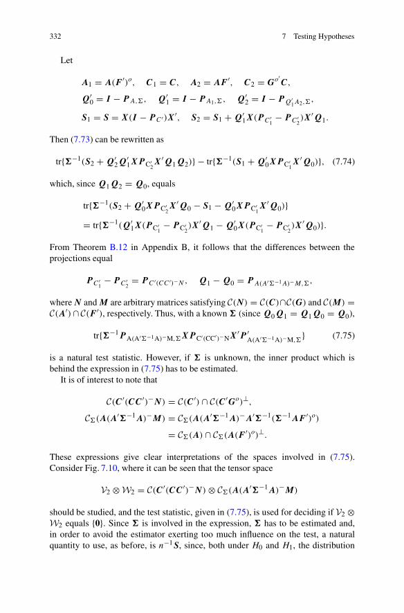
332 7 Testing Hypotheses
Let
A1 = A(F ′)o, C1 = C, A2 = AF ′, C2 = Go′C,
Q′0 = I − P A,, Q′
1 = I − PA1,, Q′2 = I − P Q′
1A2,,
S1 = S = X(I − P C ′)X′, S2 = S1 + Q′1X(P C ′
1− P C ′
2)X′Q1.
Then (7.73) can be rewritten as
tr{�−1(S2 + Q′2Q
′1XP C′
2X′Q1Q2)} − tr{�−1(S1 + Q′
0XP C′1X′Q0)}, (7.74)
which, since Q1Q2 = Q0, equals
tr{�−1(S2 + Q′0XP C′
2X′Q0 − S1 − Q′
0XP C′1X′Q0)}
= tr{�−1(Q′1X(P C′
1− P C′
2)X′Q1 − Q′
0X(P C′1− P C′
2)X′Q0)}.
From Theorem B.12 in Appendix B, it follows that the differences between theprojections equal
PC ′1− P C ′
2= P C ′(CC ′)−N, Q1 − Q0 = P A(A′−1A)−M,,
where N and M are arbitrary matrices satisfying C(N) = C(C)∩C(G) and C(M) =C(A′) ∩ C(F ′), respectively. Thus, with a known � (since Q0Q1 = Q1Q0 = Q0),
tr{�−1P A(A′−1A)−M,XP C′(CC′)−NX′P ′A(A′−1A)−M,
} (7.75)
is a natural test statistic. However, if � is unknown, the inner product which isbehind the expression in (7.75) has to be estimated.
It is of interest to note that
C(C′(CC′)−N) = C(C′) ∩ C(C′Go)⊥,
C(A(A′�−1A)−M) = C(A(A′�−1A)−A′�−1(�−1AF ′)o)
= C(A) ∩ C(A(F ′)o)⊥.
These expressions give clear interpretations of the spaces involved in (7.75).Consider Fig. 7.10, where it can be seen that the tensor space
V2 ⊗ W2 = C(C′(CC′)−N) ⊗ C(A(A′�−1A)−M)
should be studied, and the test statistic, given in (7.75), is used for deciding if V2 ⊗W2 equals {0}. Since � is involved in the expression, � has to be estimated and,in order to avoid the estimator exerting too much influence on the test, a naturalquantity to use, as before, is n−1S, since, both under H0 and H1, the distribution

7.8 A “Trace Test” for the BRM , H0 : FBG = 0 Against Unrestricted B 333
(a) (b)
Fig. 7.10 Consider the BRM model in (7.63). A decomposition is presented of the whole spaceaccording to the design and the restrictions FBG = 0. In (a), � is known, whereas in (b), �
has been replaced by 1nS. The decomposition in (a) is based on the subspaces V1 = C(C ′Go),
V2 = C(C′Go)⊥ ∩ C(C ′), V3 = C(C ′)⊥, W1 = C(A(F ′)o), W2 = C(A(F ′)o)⊥ ∩ C(A) andW3 = C(A)⊥. In (b), the subspaces V1, V2 and V3 are the same as in (a), whereas the within-individuals decomposition is based on ˜W1 = CS(A(F ′)o), ˜W2 = CS(A(F ′)o)⊥ ∩ CS(A) and˜W3 = CS(A)⊥
of S is independent of B. Note that when constructing the likelihood ratio test inSect. 7.3, different estimators of the inner product were obtained under H0 and H1,i.e. S1 andS2, defined in Sect. 7.3, were utilized. In the present situation, the statisticwas derived by first assuming � to be known and then replacing the dispersion withn−1S; i.e. the same estimator was chosen irrespective of the hypothesis, which in away makes sense since we are interested only in B and not in �. Hence, the nextproposition has been motivated.
Proposition 7.3 For the BRM presented in Definition 2.1, let the null hypothesisH0 : FBG = 0 be tested against H1: B unrestricted. Let S be defined in (7.71),and N and M be matrices satisfying C(N) = C(G) ∩ C(C) and C(M) = C(A′) ∩C(F ′), respectively. A test statistic is given by
T4 = tr{S−1P A(A′S−1A)−M,SXP C′(CC′)−NX′P ′A(A′S−1A)−M,S}.
The hypothesis is rejected when the observed value of T4 is large.
Theorem 7.12 For the BRM presented in Definition 2.1, let the null hypothesisH0 : FBG = 0 be tested against H1: B unrestricted. Under H0 the distributionfor the test statistic T4, presented in Proposition 7.3, is independent of � and B.
Proof Under H0 the statistic T4 equals
T4 = tr{S−1P A(A′S−1A)−M,S(X − ABC)P C′(CC′)−N(X − ABC)′P ′A(A′S−1A)−M,S}

334 7 Testing Hypotheses
and the distribution of S is functionally independent of B, as well as independent of
(X − ABC)PC ′(CC ′)−N .
If one uses the factorization A′ = T (I r(A) : 0)�′�1/2, where T is a non-singularmatrix and � is an orthogonal matrix, it follows from the definition of T4 that underH0 its distribution is independent of both � and B. Thus, the theorem has beenestablished. ��Theorem 7.13 Let T4 be defined in Proposition 7.3, and let the constants c0;n,s andci;n,s,t , i = 1, 2, 3, be presented in Definition B.1 (i)–(iv) of Appendix B, Sect. B.15.Moreover, put H = A(F ′)o, rN = r(N), rA = r(A), rC = r(C) and rH = r(H ).Then
(i) E[T4] = r(N)((p − rH )c0;n−r(C),p−rH − (p − rA)c0;n−rC,p−rA)
+c0;n−rC,p−rH tr{(H o′�H o)−H o′
ABN(N ′(CC′)−N)−N ′B ′A′H o};(ii) under H0
D[T4] = c1 + c2 − 2c3 − E[T4]2,
where
E[T4] = r(N)((p − rH )c0;n−r(C),p−rH − (p − rA)c0;n−rC ,p−rA),
c1 = r2N(p − rA)2c1;n−rC ,p−rA + r2
N((p − rA) + (p − rA)2)c2;n−rC ,p−rA
+2rN(p − rA)c1;n−rC ,p−rA + 2rN ((p − rA) + (p − rA)2)c2;n−rC ,p−rA ,
c2 = r2N(p − rH )2c1;n−rC ,p−rH + r2
N((p − rH ) + (p − rH )2)c2;n−rC ,p−rH
+2rN(p − rH )c1;n−rC ,p−rH + 2rN((p − rH ) + (p − rH )2)c2;n−rC ,p−rH ,
c3 = r2N(p − rA)2c1;n−rC ,p−rA,p−rH + 2r2
N(p − rA)c2;n−rC ,p−rA,p−rH
+r2N(p − rA)(rA − rH )c3;n−rC ,p−rA,p−rH
+2rN(p − rA)c1;n−rC ,p−rA,p−rH
+2rN((p − rA) + (p − rA)2)c2;n−rC ,p−rA,p−rH .
Proof Since (see Appendix B, Theorem B.13)
P A(A′S−1A)−M,S = P A,S − P A(F ′)o,S = P ′(A(F ′)o)o,S−1 − P ′
Ao,S−1,
it follows, by assuming the generators of the orthogonal complements to be of fullrank, that
T4 = tr{(H o′SH o)−1H o′
XP C′(CC′)−NX′H o}−tr{(Ao′
SAo)−1Ao′XP C′(CC′)−NX′Ao}.

7.8 A “Trace Test” for the BRM , H0 : FBG = 0 Against Unrestricted B 335
Thus, since S and XP C ′(CC ′)−N are independent, statement (i) follows by applica-tion of Theorems B.20 (ii) and B.21 (i) in Appendix B.
Turning to statement (ii), since D[T4] = E[T 24 ]−E[T4]2, the expectation E[T 2
4 ]has to be determined. Let T4 = v − u, where
u = tr{(Ao′SAo)−1Ao′
XP C′(CC′)−NX′Ao},v = tr{(H o′
SH o)−1H o′XP C′(CC′)−NX′H o}.
Then E[T 24 ] = E[u2] + E[v2] − 2E[uv] and each of these terms has to be
determined. Since XP C ′(CC ′)−NX′ is independent of S it is noted, as whendiscussing T3 (see Appendix B, Theorem B.19 (vii)), that
E[(XPC ′(CC ′)−NX′)⊗2] = r2N� ⊗ � + rN(Kp,p(� ⊗ �) + vec�vec′�).
This relation leads to
E[u2] = r2N tr{E[(Ao′
SAo)−1 ⊗ (Ao′SAo)−1]Ao′
�Ao ⊗ Ao′�Ao}
+2rN tr{E[(Ao′SAo)−1Ao′
�Ao(Ao′SAo)−1Ao′
�Ao]}.
Hence, using Appendix B, Theorem B.21 (iii) and (v) it can be shown thatc1 = E[u2]. Similarly, the expectation for v2 can be obtained and c2 = E[v2].Finally, E[uv] is to be determined. However, using Theorems B.19 (vii) and B.25in Appendix B, as well as copying the calculations for obtaining E[u2], yieldsc3 = E[uv], which establishes the theorem. ��Proposition 7.4 For the BRM presented in Definition 2.1, let the null hypothesisH0 : FBG = 0 be tested against H1: B unrestricted. The corresponding teststatistic T4 is given by Proposition 7.3. Then the hypothesis connected to T4 isrejected at approximate significance level α if P(T4o ≥ aχ2[f ]) ≤ α, where T4o
is the observed value of T4, [f ] denotes the integer part of either f or f + 1 andthe integer part which is closest to f is chosen;
a = c1 + c2 − 2c3 − c20
2c0, f = 2c2
0
c1 + c2 − 2c3 − c20
,
where c0 = E[T4] and c1 – c3 are presented in Theorem 7.13.
Proof As in Proposition 7.2, the coefficients a and f are obtained by solving
E[T4] = af, D[T4] = 2a2f,
which via Theorem 7.13 then suggests the statement. ��

336 7 Testing Hypotheses
Now the proposition is illustrated via one of our data sets which has been usedseveral times before.
Example 7.10 Our main interest is to compare the “trace test” with the likelihoodratio test. Therefore, consider the Potthoff and Roy data presented in Table 1.2,which have been analysed in Example 7.2, among other places in the book. LetX = ABC + E, whose matrices have previously been defined. In particular, notethat
A =
⎛
⎜
⎜
⎝
1 8 641 10 1001 12 1441 14 196
⎞
⎟
⎟
⎠
, C = (1′11 ⊗ (1 : 0)′ : 1′
16 ⊗ (0 : 1)′),
meaning that the growth for both the girls and the boys is modelled with a second-order polynomial.
In Example 7.2, three tests were carried out using the following hypotheses:
(i) no quadratic term in ABC;(ii) only girls follow a quadratic growth model;
(iii) no growth exists for both the boys and the girls between age 8 and age 14.
Both the hypotheses related to statement (i) and statement (ii) were deemed to benon-significant when performing a likelihood ratio test, while the hypothesis linkedto statement (iii) was rejected, which was in accordance with our expectations.
Concerning the “trace-test”, the results are in agreement. For statement (i) it isobtained that T4o = 0.1 and T4o/a = 1.4, which are non-significant since the valuesof the test statistics are below χ2
0.05(3) = 7.8. However, the exact probabilitiesfor rejection differ somewhat between the likelihood ratio test (p = 0.32) and the“trace test” (p = 0.67). This discrepancy may be due to the ad hoc procedureimplemented when deriving the “trace test” statistic or the relatively crude methodused for technically determining the probability for the “trace test”.
For statement (ii) the corresponding numbers are T4o = 0.1, T4o/a = 1.5 andχ2
0.05(2) = 6.0, and thus this test is not rejected. The rejection probabilities for thelikelihood ratio test and the “trace test” are given by p = 0.14 and p = 0.34,respectively.
For the third hypothesis, presented in statement (iii), i.e. the most extremehypothesis, the following were obtained: T4o = 5.1, T4o/a = 82.4 and χ2
0.05(2) =6.0. Both the “trace test” and the likelihood ratio test provide very small rejectionprobabilities. ��

7.9 A “Trace Test” for the BRM , H0 : F iBGi = 0, i = 1, 2, C(F ′1) ⊆. . . 337
7.9 A “Trace Test” for the BRM , H0 : FiBGi = 0, i = 1, 2,C(F ′
1) ⊆ C(F ′2), Against Unrestricted B
As when performing tests with the help of the likelihood ratio criterion in Sect. 7.4and other places in the book, the condition C(F ′
1) ⊆ C(F ′2) is supposed to hold. The
reason for assuming such an condition is that, as before, the theory developed forthe class of EBRM3
B is going to be utilized. Note that F iBGi = 0, i = 1, 2, withC(F ′
1) ⊆ C(F ′2), is equivalent to
B = (F ′2)
o�1 + (F ′1 : (F ′
2)o)o�3G
o′2 + F ′
1�4(G1 : G2)o′,
where �i are new unknown parameters which have to be estimated and, of course,C((G1 : G2)
o) ⊆ C(Go2). Thus the reparametrization implies that the mean structure
of the BRM under H0 becomes
E[X] = ABC = A(F ′2)
o�1C + A(F ′1 : (F ′
2)o)o�3Go′2 C + AF ′
1�4(G1 : G2)o′C,
i.e. an EBRM3B . For the time being, suppose that the dispersion matrix � is
known. The following notations, also used in Sect. 7.4, will be applied, but nowthe projections are solely functions of �:
A1 = A(F ′2)
o, C1 = C, A2 = A(F ′1 : (F ′
2)o)o, C2 = Go′
2 C,
A3 = AF ′1, C3 = (G1 : G2)
o′C,
S3 = S2 + P ′(A1:A2)o,−1X(PC ′
2− PC ′
3)X′P (A1:A2)o,−1,
S2 = S1 + P ′Ao
1,−1X(P C ′
1− P C ′
2)X′P Ao
1,−1, S1 = S = X(I − P C ′1)X′,
Q1 = I − P ′A1,
, Q2 = I − P ′Q′
1A2,,
Q3 = I − P ′Q′
2Q′1A3,
, Q1Q2Q3 = P Ao,−1 .
Under the alternative hypothesis, i.e. with an unrestricted mean assumed to hold, theestimated mean equals (e.g. see Sect. 2.4)
EH1[X] = P A,XP C ′,
whereas from (2.39)
EH0[X] = (I − Q′1)XP C ′
1+ (I − Q′
2)XP C ′2+ (I − Q′
3)XP C ′3. (7.76)

338 7 Testing Hypotheses
Fig. 7.11 The dotted area corresponds to H0: F iBGi = 0, i = 1, 2, in the BRM , where C(F ′1) ⊆
C(F ′2). Furthermore, W1 = C•(A(F ′
2)o), W2 = C•(A(F ′
1)o) ∩ C•(A(F ′
2)o)⊥, W3 = C•(A) ∩
C•(A(F ′1)
o)⊥, W4 = C•(A)⊥, V1 = C(C ′(G1 : G2)o), V2 = C(C ′Go
2) ∩ C(C′(G1 : G2)o)⊥,
V3 = C(C′) ∩ C(C ′Go2)
⊥ and V4 = C(C ′)⊥
Hence, similar to when tests were performed within the BRM , in Sect. 7.8, a tracetest statistic can be constructed via
tr{�−1(X − EH0[X])()′} − tr{�−1(X − EH1[X])()′}. (7.77)
In Sect. 7.8, it was relatively easy to simplify the test statistic. Because EH0[X] andEH1[X] are built up with the help of projections of observations on certain spaces,it makes sense to consider the corresponding spaces and their decompositions. Infact, what are needed are the projections of spaces indicated in Fig. 7.11 (the dottedarea), which are in agreement with the construction of Fig. 7.7.
Now, instead of performing a large number of calculations, the idea is to relyon one’s intuition. Based on Fig. 7.11, the spaces which are involved in the test aregiven by
V2 ⊗ W3 + V3 ⊗ (W2 + W3), (7.78)
where Vi and Wi , i = 2, 3, are defined in Fig. 7.11. The test which will beconstructed is to some extent a goodness-of-fit test which will help us to decideif the space given in (7.78) differs from {0}. What is needed to construct the test isthe construction of projections on the spaces in (7.78). Firstly, note that Q′
1, Q′2Q
′1
and Q′3Q
′2Q
′1 in (7.77) and (7.76) are all projectors and
C(Q′1) = C(A1)
⊥, C(Q′2Q
′1) = C(A1 : A2)
⊥,
C(Q′3Q
′2Q
′1) = C(A1 : A2 : A3)
⊥ = C(A)⊥.
Moreover,
C(A1)⊥ = C(A1)
⊥ ∩ C(A) + C(A)⊥,
C(A1 : A2)⊥ = C(A1 : A2)
⊥ ∩ C(A) + C(A)⊥,
C(A1 : A2 : A3)⊥ = C(A)⊥,

7.9 A “Trace Test” for the BRM , H0 : F iBGi = 0, i = 1, 2, C(F ′1) ⊆. . . 339
and let
V2 = C(N1) = C(C′Go2) ∩ C(C′(G1 : G2)
o)⊥,
V3 = C(N2) = C(C′) ∩ C(C′Go2)
⊥,
C(M1) = C(A) ∩ C(A(F ′1)
o)⊥,
C(M2) = C(A) ∩ C(A(F ′2)
o)⊥,
with the corresponding projections
P N1 = P C ′Go2− P C ′(G1:G2)o , P N2 = P C ′ − PC ′Go
2,
P M1, = P A, − P A1(F′1)
o,, P M2, = P A, − P A1(F′2)
o,.
Therefore, the test statistic presented in (7.77), where � is known, equals
tr{�−1((P A, − P A1(F′1)
o,)X(P C′Go2− P C′(G1:G2)o)X′
+(P A, − P A1(F′2)
o,)X(P C ′ − P C ′Go2)X′)}.
Since the distribution of S does not depend on B, either under H0 or under H1,the same argument as that applied when obtaining T3 in Proposition 7.1 can beused; i.e. replacing � by n−1S, in order to present a test statistic for the hypothesisinvolving the bilinear restrictions F iBGi = 0, i = 1, 2, and C(F ′
1) ⊆ C(F ′2) is a
natural procedure.
Proposition 7.5 For the BRM presented in Definition 2.1, let the null hypothesisH0 : F iBGi = 0, i = 1, 2, C(F ′
1) ⊆ C(F ′2), be tested against H1: B unrestricted.
Let S be defined in (7.71). A test statistic is given by
T5 = T51 + T52,
where
T51 = tr{S−1(P A,S − P A(F′1)
o,S)X(P C′Go2− P C′(G1:G2)o)X′},
T52 = tr{S−1(P A,S − P A(F′2)
o,S)X(P C′ − P C′Go2)X′}.
The hypothesis may be rejected if any of the observed values of T51, T52 or T5 islarge.
The statistics T51 and T52 are also test statistics. In particular, they are both positiveand, therefore, it is possible to consider them separately. From Proposition 7.5, since
PA,S − P A(F ′2)
o,S = P A(A′S−1A)−M, P C ′ − PC ′Go2
= PC ′(CC ′)−N,

340 7 Testing Hypotheses
where C(M) = C(A′) ∩ C(F ′2) and C(N) = C(C) ∩ C(G2), it follows that T52
tests H0: F 2BG2 = 0 in the BRM against B being arbitrary. Moreover, T51is a test statistic for testing H0: F 1BG1 = 0 in the BRM given BG2 = 0.The latter statement follows from the fact that E[X] = ABC = A�Go′
2 C
for some �, and F 1BG1 = 0 is equivalent to F 1�Go′2 G1 = 0. Furthermore,
C(Go2(G
o′2 G1)
o) = C(G1 : G2)⊥, which altogether implies the expression for T51.
It is also worth noting that X(P C ′Go2− P C ′(G1:G2)o)X
′ and X(P C ′ − P C ′Go2)X′ are
independently distributed. This implies that T51 and T52 are uncorrelated, and givenS, also independent.
Now a few results will be presented without proofs, since the statements can beverified using the same procedure as was applied in Sect. 7.8.
Theorem 7.14 For the BRM presented in Definition 2.1, let the null hypothesisH0 : F iBGi = 0, i = 1, 2, C(F ′
1) ⊆ C(F ′2), be tested against H1: B
unrestricted. Under H0 the test statistics T51 and T52, presented in Proposition 7.5,are functionally independent of B and �.
Theorem 7.15 Let T51 and T52 be defined in Proposition 7.5, and let the constantsc0;n,s and ci;n,s,t , i = 1, 2, 3, be given in Definition B.1 (i)–(iv) of Appendix B,Sect. B.15. Moreover, letN1 andN2 be any matrices satisfying C(N1) = C(Go′
2 C)∩C(Go′
2 G1) and C(N2) = C(C) ∩ C(G2), respectively, and let H 1 = A(F ′1)
o, H 2 =A(F ′
2)o, rH1 = r(H 1), rH2 = r(H 2), rA = r(A) and rC = r(C). Then
(i)
E[T52] = rN2 ((p − rH2 )c0;n−r(C),p−rH2− (p − rA)c0;n−rC,p−rA)
+c0;n−rC,p−rH2tr{(Ho′
2 �H o2)
−H o′2 ABN2(N
′2(CC′)−N2)−N ′
2B′A′H o
2};
(ii) under H0
D[T52] = c1 + c2 − 2c3 − E[T52]2,
where
E[T52] = rN2((p − rH2)c0;n−r(C),p−rH2− (p − rA)c0;n−rC,p−rA),
c1 = r2N2
(p − rA)2c1;n−rC,p−rA + r2N2
((p − rA) + (p − rA)2)
×c2;n−r(C),p−r(A) + 2rN2(p − rA)c1;n−rC,p−rA
+2rN2((p − rA) + (p − rA)2)
×c2;n−rC,p−rA,

7.9 A “Trace Test” for the BRM , H0 : F iBGi = 0, i = 1, 2, C(F ′1) ⊆. . . 341
c2 = r2N2
(p − rH2)2c1;n−rC,p−rH2
+ r2N2
((p − rH2) + (p − rH2)2)
×c2;n−rC,p−rH2+ 2rN2(p − rH2)c1,n−rC,p−rH2
+2rN2((p − rH2) + (p − rH2)2)c2;n−rC,p−rH2
,
c3 = r2N2
(p − rA)2c1;n−rC,p−rA,p−rH2+ 2r2
N2(p − rA)c2;n−rC,p−rA,p−rH2
+r2N2
(p − rA)(rA − rH2)c3;n−r(C),p−rA,p−rH2
+2rN2(p − rA)c1;n−rC,p−rA,p−rH2
+2rN2((p − rA) + (p − rA)2)c2;n−rC,p−rA,p−rH2;
(iii)
E[T51] = rN1 ((p − rH1 )c0;n−r(C),p−rH1− (p − rA))c0;n−rC,p−rA
+c0;n−rC,p−rH1tr{Ho′
1 �H o1)
−Ho′1 ABN1(N
′1(CC′)−N1)−N ′
1B′A′Ho
1};
(iv) under H0
D[T51] = c1 + c2 − 2c3 − E[T51]2,
where
E[T51] = rN1 ((p − rH1 )c0;n−r(C),p−rH1− (p − rA))c0;n−rC ,p−rA,
c1 = r2N1
(p − rA)2c1;n−rC ,p−rA + r2N1
((p − rA) + (p − rA)2)c2;n−r(C),p−r(A)
+ 2rN1 (p − rA)c1;n−rC ,p−rA + 2rN1 ((p − rA) + (p − rA)2)c2;n−rC ,p−rA,
c2 = r2N1
(p − rH1 )2c1;n−rC ,p−rH1
+ r2N1
((p − rH1) + (p − rH1)2)c2;n−rC ,p−rH1
+ 2rN1 (p − rH1 )c1;n−rC ,p−rH1+ 2rN1 ((p − rH1) + (p − rH1 )
2)c2;n−rC ,p−rH1,
c3 = r2N1
(p − rA)2c1;n−rC ,p−rA,p−rH1+ 2r2
N1(p − rA)c2;n−rC ,p−rA,p−rH1
+ r2N1
(p − rA)(rA − rH1)c3;n−r(C),p−rA,p−rH1+2rN1 (p − rA)c1;n−rC ,p−rA,p−rH1
+ 2rN1 ((p − rA) + (p − rA)2)c2;n−rC ,p−rA,p−rH1.
Proposition 7.6 Let the test statistic T52 be given by Proposition 7.5. Then thehypothesis connected to T52 is rejected at approximate significance level α ifP(T52o ≥ aχ2[f ]) ≤ α, where T52o is the observed value of T52, [f ] denotes theinteger part of either f or f +1 and the integer part which is closest to f is chosen;
a = c1 + c2 − 2c3 − c20
2c0, f = 2c2
0
c1 + c2 − 2c3 − c20
,
where c0 = E[T52] and c1 – c3 are presented in Theorem 7.15 (i) and (ii).

342 7 Testing Hypotheses
Proposition 7.7 Let the test statistic T51 be given by Proposition 7.5. Then thehypothesis connected to T51 is rejected at approximate significance level α ifP(T51o ≥ aχ2[f ]) ≤ α, where T51o is the observed value of T51, [f ] denotes theinteger part of either f or f + 1 and the the integer part which is closest to f ischosen;
a = c1 + c2 − 2c3 − c20
2c0, f = 2c2
0
c1 + c2 − 2c3 − c20
,
where c0 = E[T51] and c1 – c3 are presented in Theorem 7.15 (iii) and (iv).
Example 7.11 The melatonin data generated in Example 7.3 are considered onefinal time. In Example 7.8 the likelihood ratio test was carried out for these data.More precisely, for the BRM , H0: F iBGi = 0, i = 1, 2, was tested againstB unrestricted. The likelihood ratio statistic equals a product, λ1λ2, of two teststatistics. For these tests, λ1 tests H0 : F 2BG2 = 0 versus B unrestricted, whichturned out to be far below the critical value, while λ2, which tests H0 : F 1BG1 = 0given that F 2BG2 = 0, was not significant.
Concerning the “trace-test” for the hypothesis H0: F iBGi = 0, i = 1, 2, versusB unrestricted, it follows from Propositions 7.6 and 7.7 that the test statistics T52, fortesting H0: F 2BG2 = 0 versus B unrestricted, and T51, for testing H0: F 1BG1 = 0versus BG2 = 0, are of interest. Note that T52 corresponds to λ1, mentioned above.
The results of the “trace-test” are as follows: T52o = 1.1, T52o/a = 22.0 >
χ20.05(1) = 3.84, T51o = 0.03 and T51o/a = 0.6 < χ2
0.05(1) = 3.84. Thus, thereis a very strong agreement between the likelihood ratio test and the “trace-test”.Note that three parameters are put to zero under the null hypothesis and that thishypothesis is tested via two chi-square distributions which both have one degree offreedom. From an asymptotic point of view this is somewhat unnatural and shouldbe exploited further. ��
7.10 The Likelihood Ratio Test Versus the “Trace Test”
Firstly, it is noted that if the dispersion matrix � is known, the likelihood ratio testand the “trace test” for a given hypothesis connected to the BRM , with restrictionson the mean, will yield identical test statistics. However, a known � will neveroccur and when � is unknown, the construction of the two types of tests culminatesin different tests.
The likelihood ratio procedure considers the whole space, i.e. a tensor spacewhich consists of the within-individuals subspace and the between-individualssubspace. Moreover, the likelihood ratio procedure is a precise mathematicalformulation of the testing problem and has for a couple of centuries been known tobe the best test from an asymptotic point of view. However, with many parametersbeing included in a model, there are situations where the likelihood ratio test is

7.11 Testing an EBRM3B Against a BRM 343
not useful, since, for example, the test may reject the null hypothesis too often.There can also be a problem understanding what is really being tested when manyparameters appear in the model, in particular when there are several nuisanceparameters in the model.
In Sects. 7.3–7.7, likelihood ratio tests of hypotheses concerning B in the BRM
were mainly of interest, whereas � played a secondary role; i.e. knowledge about� was only applied when evaluating the distribution of B. In the likelihood ratiotest the maximum likelihood estimator of � was used whereas for the “trace test” itwas decided to use n−1S. Since n−1S and the maximum likelihood estimator of �
both converge to � with the same “speed”, the two different testing approachesare asymptotically equivalent. However, small sample comparisons between theapproaches have yet to be performed. One advantage of the “trace test”, whenn−1S is used, is that the spaces which are involved in the construction of the teststatistic are easier to interpret than the projections used in the construction of thelikelihood ratio statistic, where some kind of conditional approach is applied; forexample see Sect. 7.3. Moreover, when considering H0: F iBGi = 0, i = 1, 2,C(F ′
1) ⊆ C(F ′2), in the BRM , the derivation and the construction of the test statistic
are more straightforward for the “trace test” than for the likelihood ratio test.It can be mentioned that the “trace test” is a goodness-of-fit test in the sense that it
compares the fit under H0 with the fit under H1, i.e. it highlights the difference of fitunder H0 and H1. The drawback of “trace tests” is that their distributions and powerfor various alternatives have not yet been studied in detail, whereas the likelihoodratio test has been scrutinized with respect to different statistical properties. In theprevious sections, we have been relying on some ad hoc approximations, whichseems to work, but no real proofs are given. On the other hand, although likelihoodratio statistics are associated with certain errors no sharp upper error bounds areavailable for the tests of the hypotheses in Sects. 7.3–7.7.
7.11 Testing an EBRM3BAgainst a BRM
Now we return to exploiting likelihood ratio tests, and the results of Sects. 7.6 and7.7 will be slightly extended. The reason is that in the next section, restrictions ofa different type than F iBGi = 0, i = 1, 2, are considered and the results will relyon the present section. In the previous sections, restrictions were put on B in theBRM , X = ABC + E, through F iBGi = 0, i = 1, 2, C(F 2) ⊆ C(F 1). In thissection it is assumed that under H0
E[X] = A1B1C1 + A2B2C2 + A3B3C3, C(C′3) ⊆ C(C′
2) ⊆ C(C′1), (7.79)
where B i , i = 1, 2, 3, are the parameters of interest. Under the alternativehypothesis we have
E[X] = ABC,

344 7 Testing Hypotheses
where in particular C(A1 : A2 : A3) ⊆ C(A), C(C1) ⊆ C(C) and B is completelyunknown, i.e. no restrictions apply to B. Thus, an EBRM3
B is tested against aBRM . From Theorems 3.1 and 3.2, it follows that the likelihood ratio test statisticfor testing (7.79) is equivalent to
λ2n = |�H0 |
|�H1 |= |S3 + Q
′3Q
′2Q
′1XPC ′
3X′
Q1Q2
Q3||S + P ′
Ao,S−1XPC ′X′P Ao,S−1 | , (7.80)
where the notation follows that of Sect. 7.4, except that Ai , i = 1, 2, 3, and Ci ,i = 1, 2, 3, are arbitrary known matrices following the conditions
C(C′3) ⊆ C(C′
2) ⊆ C(C′1) ⊆ C(C′),
C(A1 : A2 : A3) ⊆ C(A). (7.81)
Let ˜A be any matrix such that
C(˜A) = C(A1 : A2 : A3).
As in Sects. 7.6 and 7.7, the test statistic in (7.80) can be factorized, but this time itis natural to work with three factors (see Fig. 7.12):
λ = λ1λ2λ3,
where
λ
2n1 =
|S1 + P ′˜Ao,S−1
1XP C ′
1X′P
˜Ao,S−11
||S + P ′
Ao,S−1XP C ′X′PAo,S−1 | , (7.82)
λ
2n2 =
|S2 + P ′˜Ao,S−1
2XP C ′
2X′P
˜Ao,S−12
||S1 + P ′
˜Ao,S−11
XP C ′1X′P
˜Ao,S−11
| , (7.83)
λ
2n3 =
|S3 + P˜Ao,S−1
3XP C ′
3X′P
˜Ao,S−13
||S2 + P ′
˜Ao,S−12
XP C ′2X′P
˜Ao,S−12
| , (7.84)
and for clarity S1, S2 and S3 are also given:
S1 = X(I − P C ′1)X′,
S2 = S1 + P ′Ao
1,S−11
X(P C ′1− P C ′
2)X′P
Ao1,S
−11
,
S3 = S2 + P ′(A1:A2)o,S
−12
X(P C ′2− PC ′
3)X′P
(A1:A2)o,S−1
2.

7.11 Testing an EBRM3B Against a BRM 345
Fig. 7.12 In (a), the dottedarea corresponds to thelikelihood ratio test H0:E[X] = A1B1C1 +A2B2C2 + A3B3C3 againstH1: E[X] = ABC, whereC(A1 : A2 : A3) ⊆ C(A) andC(C ′
3) ⊆ C(C ′2) ⊆ C(C ′
1) ⊆C(C). The test statistic λ ispresented in (7.80). In (b), thetest statistic λ1 in (7.82) isillustrated, and (c) and (d)show what is tested with λ2and λ3, respectively.Furthermore, V1 = C(C′
3),V2 = C(C′
2) ∩ C(C ′3)
⊥,V3 = C(C′
1) ∩ C(C2)⊥,
V4 = C(C1) ∩ C(C ′)⊥ andV5 = C(C′)⊥
V1 V2 V3 V4 V5
(a)
V1 V2 V3 V4 V5
(b)
V1 V2 V3 V4 V5
(c)
V1 V2 V3 V4 V5
(d)
Note that λ2 and λ3 correspond to (7.53) and (7.54), respectively, and Theo-rem 7.8 describes how the tests based on λ2 and λ3 should be performed. In Fig. 7.12the three different test statistics are illustrated. Here it can be seen that λ1 tests ifthe space (C(C′
1)⊥ ⊗ C(˜A)⊥) ∩ (C(C) ⊗ C(A)) equals {0}. If this test is rejected,
then the overall hypothesis about the EBRM3B against the BRM is also rejected.
However, if it is not rejected, then it makes sense to investigate λ2, which tests ifthe space (C(C′
2)⊥ ∩ C(C′
1)) ⊗ (C(A1)⊥ ∩ C(˜A)) equals {0}. Moreover, if λ2 is not
rejected either, then the test statistic λ3 should be considered, and in this case it willbe tested whether the space (C(C′
3)⊥ ∩ C(C′
2)) ⊗ (C(A1 : A2)⊥ ∩ C(˜A)) equals {0},
given that (C(C′2)
⊥ ∩ C(C′1)) ⊗ (C(A1)
⊥ ∩ C(˜A)) = {0}.Before deriving the approximating distributions of the three test statistics
mentioned above, it can be noted that if one wants to simplify the technicaltreatment, which, however, is not necessary, � can be replaced by I without anyloss of generality; i.e. the distribution of the test statistic does not depend on �.Therefore, in order to indicate that � = I is assumed to hold, X is replaced byY ∼ Np,n(0, Ip, In), Si by V i (defined as the matrix where in Si the matrix X
has been replaced by Y ), and S is replaced by V ∼ Wp(I , n − r(C)). Moreover,instead of Ai , i = 1, 2, 3, and A one should now have �1/2Ai and �1/2A, but itis not necessary to emphasize this. The obtained distributions will not depend onAi or A, and only the ranks of these matrices are important; these do not changewith pre-multiplication by �1/2. Now we start to derive an approximation of thedistribution of the likelihood ratio test and to consider
λ
2n1 =
|V 1 + P ′˜Ao,V −1
1YP C ′
1Y ′P
˜Ao,V −11
||V + P ′
Ao;V −1YPC ′Y ′P Ao;V −1 | . (7.85)

346 7 Testing Hypotheses
It is worth noting that in Sects. 7.6 and 7.7, the matrices satisfied C(A1 : A2 : A3) =C(A) and C(C′
1) = C(C′), and therefore in these sections it was not necessary toconsider a statistic like λ1 in (7.85). The expression in (7.85) can be rewritten as
λ
2n1 = |V 1||(˜Ao′
V 1˜Ao)−1||(˜Ao′
YY ′˜A
o)|
|V ||(Ao′V Ao)−1||(Ao′
YY ′Ao)| . (7.86)
Based on the assumption C(˜A) = C(A1 : A2 : A3) ⊆ C(A) and utilizing AppendixB, Theorem B.3 (ii)
C(˜Ao) = C(Ao) � C(H ), (7.87)
where H is a matrix of full rank satisfying C(H ) = C(A) ∩ C(˜A)⊥. Using thedecomposition in (7.87), it follows that in (7.86), ˜A
ocan be replaced by (Ao : H ).
Thus, Appendix B, Theorem B.8 (iv) establishes that
λ
2n1 = |V 1||(Ao′
V 1Ao)−1||H ′V 1H − H ′V 1A
o(Ao′V 1A
o)−1Ao′V 1H |−1
|V ||(Ao′V Ao)−1|
×|(Ao′YY ′Ao)||H ′YY ′H − H ′YY ′Ao(Ao′
YY ′Ao)−1Ao′YY ′H |
|(Ao′YY ′Ao)| .
Hence, the test statistic can be factored into
λ1 = λ11λ12,
where
λ
2n11 = |V 1||(Ao′
V 1Ao)−1|
|V ||(Ao′V Ao)−1| , (7.88)
λ
2n12 = |H ′YY ′H − H ′YY ′Ao(Ao′
YY ′Ao)−1Ao′YY ′H |
|H ′V 1H − H ′V 1Ao(Ao′
V ′1A
o)−1Ao′V ′
1H |
= |H ′A(A′(YY ′)−1A)−1A′H ||H ′A(A′V −1
1 A)−1A′H | , (7.89)
and A is any matrix of full rank satisfying C(A) = C(A). The appearance of twotest statistics instead of λ1 is in agreement with Fig. 7.12b.
Concerning λ
2n11 this expression is similar to (7.14). Therefore, it is possible to
copy all the calculations from (7.14) into the final expression in (7.20). The onlyissue that has to be addressed is the definition of the corresponding M and N
matrices, which are similar to those used in (7.18). It follows that N has to satisfy
PC ′ − P C ′1
= PC ′(CC ′)−N,

7.11 Testing an EBRM3B Against a BRM 347
i.e. N = C(C′1)
o. Moreover, M must satisfy
C(M) = C(A′)
and M should be of full rank. Then the result of Theorem 7.2 can be utilized.Another way of obtaining the result is to suppose that F = I in Sect. 7.3 and applyCorollary 7.1.
In the following, (7.89) is exploited. First it is noted (putting PB = P C ′(CC ′)−N ,N = C(C′
1)o), that
YY ′ = V 1 + YPBY ′,
and applying Theorem B.6 (i) in Appendix B yields (since PB is idempotent)
(YY ′)−1 = V −11 − V −1
1 YPB(PBY ′V −11 YPB + I )−1PBY ′V −1
1 .
Thus, using Appendix B, Theorem B.6 (i) once again,
(A′(YY ′)−1A)−1 = (A′V −11 A)−1 + (A′V −1
1 A)−1A′V −11 YPB(I + PBY ′V −1
1 YPB
−PBY ′V −11 A(A′V −1
1 A)−1A′V −11 YPB)−1PBY ′V −1
1 A(A′V −11 A)−1
= (A′V −11 A)−1 + (A′V −1
1 A)−1A′V −11 YPB(I + PBY ′Ao(Ao′
V 1Ao)−1Ao′
YPB)−1
×PBY ′V −11 A(A′V −1
1 A)−1.
Utilizing the above derivation, λ12 in (7.89) can be shown to equal
λ
2n12 = |I + PBY ′Ao(Ao′
V 1Ao)−1Ao′
YPB|−1|I + PBY ′Ao(Ao′V 1A
o)−1Ao′YPB
+PBY ′A(A′V −11 A)−1
×A′H (H ′A(A′V −11 A)−1A′H )−1H ′A(A′V −1
1 A)−1A′YPB|= |I + PBY ′Ao(Ao′
V 1Ao)−1Ao′
YPB|−1|I + PBY ′V −11 YPB
−PBY ′A(A′H )o((A′H )o′A′V 1A(A′H )o)−1(A′H )o
′A′YPB|
= |I + PBY ′Ao(Ao′V 1A
o)−1Ao′YPB|−1
×|I + PBY ′(A(A′H )o)o((A(A′H )o)o′V 1(A(A′H )o)o)−1(A(A′H )o)o
′YPB|.
However, λ
2n12 has the same form as the expression in (7.16). Thus, the remaining
task is to determine an M such that
P(A(A′H)o)o,V −1
1− P
Ao,V −11
= PV −1
1 A(A′V −11 A)−M,V −1
1,

348 7 Testing Hypotheses
V1 V2 V3 V4 V5
(a)
V1 V2 V3 V4 V5
(b)
Fig. 7.13 In (a), the dotted area corresponds to the likelihood ratio test statistic λ11, givenin (7.88). In (b), the test statistic λ12 in (7.89) is illustrated. Furthermore, V1 = C(C ′
3), V2 =C(C ′
2) ∩ C(C ′3)
⊥, V3 = C(C ′1) ∩ C(C2)
⊥, V4 = C(C1) ∩ C(C′)⊥ and V5 = C(C ′)⊥
implying that M can be chosen as M = A′˜A
o(see Appendix B, Theorem B.12).
Hence, with N = C′Co1 and M = A′
˜Ao, the relation in (7.20) can be utilized.
The test statistics λ11 and λ12 given in (7.88) and (7.89), respectively, areillustrated in Fig. 7.13.
Theorem 7.16 Testing an EBRM3B presented in Definition 2.2 against a BRM
presented in Definition 2.1. Under H0 the data are assumed to follow an EBRM3B
with the mean
E[X] = A1B1C1 + A2B2C2 + A3B3C3, C(C′3) ⊆ C(C′
2) ⊆ C(C′1).
Moreover, under H1 the data are modelled by a standard BRM with the mean
E[X] = ABC, C(C′1) ⊆ C(C′), C(˜A) = C(A1 : A2 : A3) ⊆ C(A).
Then the likelihood ratio test statistic λ for testing H0 against H1 can be factoredinto four components:
λ = λ11λ12λ2λ3,
where λ11, λ12, λ2 and λ3 are identified via (7.88), (7.89), (7.83) and (7.84),respectively.
Each component can be considered to be a test statistic and H0 is rejected ifone or several of the observed test statistics are in the tails of their correspondingdistributions.
The next proposition utilizes Theorem C.3 in Appendix C. Note that the resultsconcerning λ2 and λ3 stem from Theorem 7.9.

7.11 Testing an EBRM3B Against a BRM 349
Proposition 7.8 Let
c1(po, f,m) = pom(p2o + m2 − 5)
48(f − 12 (po − m + 1))2
,
c2(po, f,m) = 14608p2
om2(p2
o + m2 − 5)2
+pom(3p4o + 3m4 + 10p2
om2 − 50(p2
o + m2) + 159)
1920(f − 12 (po − m + 1))4
.
(i) Let λ11o be the observed value of λ11, given by (7.88) and used in theexpression of the likelihood ratio test, presented in Theorem 7.16. Put
to = − 2n(f − 1
2 (po − m + 1)) ln λ11o,
where f = n−r(C)−p+r(A), po = r(A) andm = r(C)−r(C1). Moreover,let c1 = c1(po, f,m) and c2 = c2(po, f,m). The hypothesis corresponding tothe statistic λ11 in Theorem 7.16 is rejected, approximately at significance levelα, if to satisfies
P {χ2pom
≥ to} + c1(1 − c1)(P {χ2pom+4 ≥ to} − P {χ2
pom≥ to})
+ c2(P {χ2pom+8 ≥ to} − P {χ2
pom≥ to}) ≤ α.
(ii) Let λ12o be the observed value of λ12, given by (7.89) and used in theexpression of the likelihood ratio test in Theorem 7.16. Put
to = 2n(f − 1
2 (po − m + 1)) ln λ12o,
where f = n − r(C) − p + r(A), po = r(A) − r(˜A) and m = r(C) −r(C1). Moreover, let c1 = c1(po, f,m) and c2 = c2(po, f,m). The hypothesiscorresponding to the statistic λ12 in Theorem 7.16 is rejected, approximatelyat significance level α, if to satisfies
P {χ2pom
≥ to} + c1(1 − c1)(P {χ2pom+4 ≥ to} − P {χ2
pom≥ to})
+ c2(P {χ2pom+8 ≥ to} − P {χ2
pom≥ to}) ≤ α.
(iii) Let λ2o be the observed value of λ2, given by (7.83) and used in the expressionof the likelihood ratio test in Theorem 7.16. Put
to = 2n(f − 1
2 (po − m + 1)) ln λ2o,

350 7 Testing Hypotheses
where f = n − r(C) − p + r(A), po = r(˜A) − r(A1) and m = r(C1) −r(C2). Moreover, let c1 = c1(po, f,m) and c2 = c2(po, f,m). The hypothesiscorresponding to the statistic λ1 in Theorem 7.8 is rejected, approximately atsignificance level α, if to satisfies
P {χ2pom
≥ to} + c1(1 − c1)(P {χ2pom+4 ≥ to} − P {χ2
pom≥ to})
+ c2(P {χ2pom+8 ≥ to} − P {χ2
pom≥ to}) ≤ α.
(iv) Let λ3o be the observed value of λ3, given by (7.84) and used in the expressionof the likelihood ratio test in Theorem 7.16. Put
to = 2n(f − 1
2 (po − m + 1)) ln λ3o,
where f = n − r(C) − p + r(A), po = r(˜A) − r(A1 : A2) and m = r(C2) −r(C3). Moreover, let c1 = c1(po, f,m) and c2 = c2(po, f,m). The hypothesiscorresponding to the statistic λ2 in Theorem 7.8 is rejected, approximately atsignificance level α, if to satisfies
P {χ2pom
≥ to} + c1(1 − c1)(P {χ2pom+4 ≥ to} − P {χ2
pom≥ to})
+ c2(P {χ2pom+8 ≥ to} − P {χ2
pom≥ to}) ≤ α.
7.12 Estimating and Testing in the BRM withF 1BG1 = F 2�G2
In this section, a new way of formulating restrictions is presented. However, it canbe worth noting that most of the mathematical treatment is not presented. The readerwho has understood the previous sections is supposed to be able to fill in the gaps,and one may regard this section as a kind of follow-up section. The restrictions forthe BRM with the mean E[X] = ABC are in this section assumed to satisfy
F 1BG1 = F 2�G2, (7.90)
where F i and Gi , i = 1, 2, are known matrices, and � and B unknown parameters.The purpose is to estimate the parameters in (7.90) and test (7.90) against B
unstructured. It is natural to consider (7.90) as a system of linear equationswhose solution is generated by free parameters (i.e. a reparametrization will takeplace), and then use knowledge about the EBRM3
B . However, before a detailedpresentation and discussion are provided, an explanatory and illustrative example isgiven.

7.12 Estimating and Testing in the BRM with F 1BG1 = F 2�G2 351
Example 7.12 Suppose that there are two samples of different types of plants wherea linear growth over time is observed by following each plant at the same timepoints, i.e.
E[Xijk] = αi + βitj , k = 1, 2, . . . , ni .
However, if αi is proportional to another factor (let us say the temperature), then
αi = θ tempi , i = 1, 2,
for some unknown θ . Thus, the following mean structure emerges:
E[Xijk] = θ tempi + βitj , i = 1, 2; j = 1, 2, . . . , p; k = 1, 2, . . . , ni .
In matrix notation the model can be written as follows:
E[X] = ABC + E, E ∼ Np,n(0,�, I ),
B =(
α1 α2
β1 β2
)
,
A′ =(
1 1 . . . 1t1 t2 . . . tp
)
, C =(
1 1 . . . 1 0 0 . . . 00 0 . . . 0 1 1 . . . 1
)
,
F 1 = (1 : 0), G2 = (temp1 : temp2),
where F 1B = θG2.If instead of two groups, there are three groups, two of which only are affected,
then
B =(
α1 α2 α3
β1 β2 β3
)
, G1 =⎛
⎝
1 00 10 0
⎞
⎠ ,
where F 1BG1 = θG2. Moreover, if αi , i = 1, 2, are affected not only bytemperature, but also by the pressure (prei), for example, then F 1BG1 = �G2,with
� = (θ1 : θ2), G2 =(
temp1 temp2pre1 pre2
)
.
��Now a few theoretical results connected to the restrictions F 1BG1 = F 2�G2 arederived. From Theorem B.10 (iv) in Appendix B, the general solution to F 1BG1 =F 2�G2 is given by
� = F−2 F 1(F
′1F
o2 : (F ′
1)o)oZ3(G1(G
′2)
o)o′G1G
−2 + (F ′
2)oZ1 + F ′
2Z2Go′2 ,
B = (F ′1F
o2 : (F ′
1)o)oZ3(G1(G
′2)
o)o′ + F ′
1Fo2Z4G
o′1 + (F ′
1)oZ5, (7.91)

352 7 Testing Hypotheses
where Zi , i = 1, 2, . . . , 6, are arbitrary matrices. These relations inform us thatthe restrictions F 1BG1 = F 2�G2 in the BRM lead to an EBRM3
B . ThereforeTheorem 3.2 is at our disposal and the next theorem can be established.
Theorem 7.17 For the BRM presented in Definition 2.1, let F 1BG1 = F 2�G2hold, where F i and Gi , i = 1, 2, are known and � and B are unknown. Then themean can be written as follows:
E[X] = A(F ′1)
oB1C + A(F ′1F
o2 : (F ′
1)o)oB2(G1(G
′2)
o)o′C + AF ′
1Fo2B3G
o′1 C,
where B i , i = 1, 2, 3, are new parameters and the model belongs to the class ofEBRM3
B . The maximum likelihood estimators of the mean parameters are given by
� = F −2 F 1(F
′1F
o2 : (F ′
1)o)oB2(G1(G
′2)
o)o′G1G
−2 + (F ′
2)oZ1 + F ′
2Z2Go′2 ,
B = (F ′1)
oB1 + (F ′
1Fo2 : (F ′
1)o)oB2(G1(G
′2)
o)o′ + F ′
1Fo2B3G
o′1 ,
where B i , i = 1, 2, 3, follow from Theorem 3.2 and Zi , i = 1, 2, are arbitrarymatrices.
Theorem 7.18 For the BRM presented in Definition 2.1, let F 1BG1 = F 2�G2hold, where F i and Gi , i = 1, 2, are known and � and B unknown. Let the meanstructure be as in Theorem 7.17. Then
(i) B3 is unique if and only if
C(AF ′1F
o2) ∩ C(A(F ′
1Fo2)
o) = {0}
and AF ′1F
o2 and C′Go
1 are of full rank;(ii) B2 is unique if and only if
C(A(F ′1)
o) ∩ C(A(F ′1F
o2 : (F ′
1)o)o) = {0},
C(A(F ′1)
o)⊥ ∩ C(A(F ′1F
o2)
o) ∩ C(A(F ′1F
o2 : (F ′
1)o)) = {0}
and A((F ′1)
o : F ′1F
o2)
o and C′(G1(G′2)
o)o are of full rank;(iii) B1 is unique if and only if
C(A(F ′1)
o) ∩ C(A(F ′1F
o2 : (F ′
1)o)o) = {0},
C(A(F ′1F
o2 : (F ′
1)o)))⊥ ∩ C(A(F ′
1Fo2)
o) ∩ C(AF ′1) = {0},
r(C) = k and A(F ′1)
o is of full rank;put H = (F ′
1Fo2 : (F ′
1)o);
(iv) � is unique if and only if
C(F ′1F 2) ⊆ C(H ) � C(A′) ∩ C(H )⊥,

7.12 Estimating and Testing in the BRM with F 1BG1 = F 2�G2 353
and both F 2 and G2 are of full rank, i.e. Zi , i = 1, 2, in � in Theorem 7.17disappear;
(v) B is unique if and only if
C(F ′1)
⊥ ∩ C(A′)⊥ = {0}, C(F 1Ho) ∩ C(F 1(A
′)o) = {0},C(F ′
1Fo2) ⊆ C(A′), r(C) = k.
Finally, the BRM with the restrictions F 1BG1 = F 2�G2 is tested againstunrestricted BRM . The goal is to utilize Sect. 7.11, where in general an EBRM3
B
was tested against a BRM .From Theorem 7.17, it follows that Ai and C i in the EBRM3
B are given by
A1 = A(F ′1)
o, C1 = C,
A2 = A(F ′1F
o2 : (F ′
1)o)o, C2 = (G1(G
′2)
o)o′C,
A3 = AF ′1F
o2, C3 = Go′
1 C.
Now two important observations can be made based on these relations: C(C′1) =
C(C′) and C(A1 : A2 : A3) = C(A). Therefore, the testing problem in Sect. 7.11can be simplified, and only λ2 and λ3 in Proposition 7.8 (iii) and (iv) have to beconsidered. It follows that the likelihood ratio test for testing (7.90) against anarbitrary B is equivalent to (see (7.80))
λ2n = |�H0 |
|�H1 |= |S3 + Q
′3Q
′2Q
′1XPC ′
3X′
Q1Q2
Q3||S + P ′
Ao,S−1XPC ′X′P Ao,S−1 | , (7.92)
where Q′3Q
′2Q
′1 = P ′
Ao,S−13
and
S3 = S2 + P ′(A1:A2)o,S
−12
X(P C ′2− P C ′
3)X′P
(A1:A2)o,S−12
,
S2 = S + P ′Ao
1,S−1X(P C ′1− P C ′
2)X′P Ao
1,S−1,
S = X(I − P C ′)X′.
Moreover,
λ = λ1λ2,
where
λ
2n1 =
|S2 + P ′Ao,S−1
2XP C ′
2X′P
Ao,S−12
||S + P ′
Ao,S−1XP C ′X′PAo,S−1 | , (7.93)

354 7 Testing Hypotheses
λ
2n2 =
|S3 + PAo,S−1
3XP C ′
3X′P
Ao,S−13
||S2 + P ′
Ao,S−12
XP C ′2X′P
Ao,S−12
| , (7.94)
leading to the next theorem.
Theorem 7.19 For the BRM presented in Definition 2.1, let F 1BG1 = F 2�G2hold, where F i and Gi , i = 1, 2, are known and � and B are unknown. Then thefollowing statements can be made.
(i) Let λ1o be the observed value of λ1, given by (7.93) and used in the factorizationof the likelihood ratio test, presented in (7.92). Put
to = 2n(f − 1
2 (po − m + 1)) ln λ1o,
where f = n − r(C) − p + r(A), po = r(A) − r(A(F ′1)
o) and m = r(C) −r(C2). Moreover, let c1 = c1(po, f,m) and c2 = c2(po, f,m) be defined inProposition 7.8. The hypothesis corresponding to the statistic λ1 is rejected,approximately at significance level α, if to satisfies
P {χ2pom
≥ to} + c1(1 − c1)(P {χ2pom+4 ≥ to} − P {χ2
pom≥ to})
+ c2(P {χ2pom+8 ≥ to} − P {χ2
pom≥ to}) ≤ α.
(ii) Let λ2o be the observed value For λ2, given by (7.94) and used in thefactorization of the likelihood ratio test, presented in (7.92). Put
to = 2n(f − 1
2 (po − m + 1)) ln λ2o,
where f = n − r(C) − p + r(A), po = r(A) − r(A(F ′1F
o2)
o) and m =r(C2) − r(C3). Moreover, let c1 = c1(po, f,m) and c2 = c2(po, f,m) bedefined in Proposition 7.8. The hypothesis corresponding to the statistic λ2 isrejected, approximately at significance level α, if to satisfies
P {χ2pom
≥ to} + c1(1 − c1)(P {χ2pom+4 ≥ to} − P {χ2
pom≥ to})
+ c2(P {χ2pom+8 ≥ to} − P {χ2
pom≥ to}) ≤ α.
Problems
1 In the Potthoff and Roy (1964) data set presented in Table 1.2, remove the out-lying individuals and perform significance tests to answer the following questions.

7.12 Estimating and Testing in the BRM with F 1BG1 = F 2�G2 355
(i) Do the observations follow a linear growth model? (ii) Do the boys and the girlsfollow the same growth model?
2 In the Potthoff and Roy (1964) data set presented in Table 1.2, replace theoutlying observations by trustworthy observations and perform significance teststo answer the following questions. (i) Do the observations follow a linear growthmodel? (ii) Do the boys and the girls follow the same growth model?
3 Construct a test, based on the likelihood ratio, for testing whether a GMANOVA +MANOVA model is a GMANOVA model (suppose an arbitrary dispersion matrix).
4 Construct a test, based on the likelihood ratio, for testing whether a GMANOVA+ MANOVA model is a GMANOVA model if � = σ 2I , where σ 2 is unknown (Bai,2009).
5 Copy Example 7.3, but choose some parameters B i , i = 1, 2, 3, and � other thanthose used in the example.
6 Why are V 1 and U1, given by (7.61) and (7.62), respectively, independentlydistributed? Give a detailed explanation.
7 Perform the same tests as those described in Example 7.10, but remove individu-als which are deemed to be outliers. Explain your choice of outliers for removal.
8 For the EBRM3B , construct a test for testing F 1B1G1 = F 2B2G2 in an
EBRM3B with the mean E[X] = A1B1C1 + A2B2C2 + A3B3C3.
9 Prove at least two of the statements in Theorem 7.18.
10 Prove Theorem 7.19.
Literature
According to Cox and Hinkley (1974, p. 82), testing hypotheses have beenperformed for more than 200 years. A relatively deep discussion of significancetesting was provided by Cox (1977), with insightful comments made by E. Spjøtvoll,S. Johansen, J.F. Bithell, W.R. van Zwet, O. Barndorff-Nielsen and M. Keuls. Bythe end of the nineteenth century, one was focusing on the problem of whetherdata fitted a specific distribution (followed a specific frequency curve), and Pearson(1900) (see also Plakett, 1983) came up with the chi-square test. Nowadays this testis also termed a goodness-of-fit test and it is a test which is carried out without analternative hypothesis. Student (1908) derived the t-distribution in order to evaluatea mean in small samples, when the variation was estimated, which later becameknown as the t-test (see also Fisher, 1925, 1939). Over many years (1912–1922,approximately, see Aldrich, 1997), Fisher developed the likelihood theory, andthis work culminated in the remarkable article, Fisher (1922), where many basicinferential concepts were introduced, including sufficiency (see also Fisher, 1920;

356 7 Testing Hypotheses
Stigler, 1973). A few years later in another seminal work, Neyman and Pearson(1928a,b) started to consider statistical testing through a null hypothesis and analternative hypothesis (see also Neyman and Pearson (1933), where a completetheory was presented). Inspired by Fisher, Neyman and Pearson (1928a) proposedto use the ratio of the likelihood corresponding to the null hypothesis and thelikelihood corresponding to the alternative hypothesis. Neyman and Pearson (1933)also considered Student’s result and showed, under Student’s assumptions, that thelikelihood ratio test was equivalent to the t-test. The links between Fisher, Neymanand Pearson and Wald (1939), who replaced the power function by the loss functionand created decision theory, are very interesting to study, but outside the scope ofthis book.
At the beginning of the 1930s, the Wishart distribution was available andHotelling (1931) derived a multivariate version of the t-distribution. Therefore,it was natural that one started to work on multivariate testing problems. Wilks(1932) was successful when using the likelihood ratio test of Neyman and Pearson(1928a,b) together with the multivariate normal distribution. The Wilks statistic(Wilks, 1935) was quickly adopted by the statistical community and, among others,Bartlett (1934) and Hotelling (1936) used it (see also Bartlett, 1939). Rao (1948)gave an important overview of multivariate testing problems in various areas and inparticular in discriminant analysis.
After Neyman and Pearson had formalized the testing of hypotheses, statisticscould be used as a tool for decision making, which was not uncontroversial.From the 1950s onwards, testing in multivariate analysis became more common.Anderson (1951) studied multivariate problems which were not direct extensionsof univariate problems, for example rank restrictions on parameters (today the term“reduced rank regression” is in use). For example, if there are three parameters, thehypothesis might be that the parameters follow a line instead of varying freely. In hisarticle from 1951, Anderson applied the likelihood ratio test. S.N. Roy had for manyyears been working on the problem of composite hypothesis when he (Roy, 1953)introduced the union intersection procedure. This testing procedure has often beenapplied in multivariate analysis. Less known is the intersection union procedure.Lehmann (1952) introduced this procedure, but for multivariate testing problems,many open questions remain (e.g. see Berger and Sinclair, 1984; Berger, 1997).Moreover, in one of the first books on multivariate analysis, written by Roy (1957),the MANOVA model was treated together with a bilinear null hypothesis, i.e. H0:FBG = 0, where F and G are known matrices and B is the parameter matrix.The alternative hypothesis was that B is unrestricted. It is interesting that a preciselikelihood ratio test could be carried out without estimating the parameters underthe null hypothesis.
Khatri (1966) was the first to present the maximum likelihood estimators forthe BRM . Moreover, in Khatri’s article from 1966, the likelihood ratio test fortesting H0: FBG = 0 in the BRM was derived, and some alternative types oftest statistics were proposed (see also Pillai, 1955; Troskie, 1971). Among thetests which were obtained was one based on the union intersection procedure. Allthe derived test statistics are functions of eigenvalues of specific sums of squares

7.12 Estimating and Testing in the BRM with F 1BG1 = F 2�G2 357
matrices. However, there are some difficult results which are not easy to apply,for example exact non-null distributions for the likelihood ratio test statistic fortesting H0: FBG = 0 (see Kabe (1975a) who followed Gleser and Olkin (1970),Nagarsenker (1977), Kabe (1986), Tang and Gupta (1986)). Asymptotic expansionsof the non-null distributions of the statistics considered by Khatri (1966) werediscussed by Fujikoshi (1973a,b, 1974a,b,c). A review of various test statistics,including the above-mentioned ones, was presented by De Waal (1976). In additionto the literature discussing the likelihood ratio testing in the BRM , there existsquite a large volume of literature connected to the test statistic Wilks �, itsdensity under the null hypothesis, and its alternative hypothesis (see, for example,Gupta 1971; Hart and Money, 1975, 1976; Gupta and Nagar, 2000; Bekker et al.,2011). Moreover, connected to the Wilks � test statistic are beta distributions andmultivariate beta distributions (see Appendix C in this book), as well as extensionsof these distributions (newer references are Nadarajah, 2005; Pham-Gia, 2008).
For the performance of multivariate analysis and, of course, for the application ofthe BRM and its extensions, simultaneous test procedures are of interest and resultshave been presented by Krishnaiah (1969, 1975). Newer works, however, mostlyconsider simultaneous confidence intervals for multiple comparisons (e.g. see Seoand Kanda, 1996). An interesting area of application for growth curve analysis andtesting is profile analysis (see Srivastava, 1987; Ohlson and Srivastava, 2010; Seoet al., 2011).
Concerning information about testing in the BRM or EBRMk• , an outstandingwork from a theoretical point of view is a monograph by Kariya (1985). Thismonograph includes theory about the statistical tests in these models which is basedon a discussion of a joint application of sufficiency and invariance. The basic ideasgo back to Gleser and Olkin (1970) and Kariya (1978) (see also Giri and Das,1988), which in turn relied on older material. The following steps for testing in theBRM were presented by Kariya (1985) (see also Muirhead, 1982, pp. 520–525):(i) consider a “natural” sufficient statistic; (ii) find the largest group which leavesthe testing problem invariant; (iii) choose a convenient maximal invariant under thegroup found; (iv) derive the distribution of the maximal invariant; (v) derive theuniform most powerful invariant test or locally best invariant test, etc.; (vi) derivean approximate distribution of the test statistic under the null hypothesis. Gleser andOlkin (1970) reduced the BRM to its canonical form (inspired by Hsu, 1941). Thenit is easy to identify the sufficient statistic, i.e. a canonical version of (XC′(CC′)−,S) and show that the statistic is not complete. Using the group considered by Gleserand Olkin (1970), Banken (1984) presented an explicit expression of the maximalinvariant. Moreover, Kariya (1978) studied a larger group (see also Muirhead, 1982,p. 524) than that studied by Gleser and Olkin (1970), and this larger group wasshown by Banken (1986) to be the largest group which leaves the testing probleminvariant. In Kariya (1985), locally most powerful invariant tests were presented.A most interesting and advanced article is that by Andersson et al. (1993), wheremathematically bilinear regression models were described via the general block-triangular group and invariance. The authors mentioned that the models belonged tothe class of the so-called totally ordered linear models (nested models) which they

358 7 Testing Hypotheses
introduced. Andersson et al. (1993) presented some results concerning likelihoodratio testing, but their main focus was directed on estimation. However, it is quiteclear that through factorization of the likelihood various types of likelihood ratiotest could have been produced. For a few examples of likelihood ratio tests, seeFujikoshi et al. (1999).
In this chapter, it is assumed that the random variables corresponding to theobservations are normally distributed. However, test statistics are often true underbroader classes of distributions; for example in addition to the normal distribution,tests can also be valid for heavy-tailed distributions. If a test statistic can beused for other distributions than the normal distribution, the test is deemed to berobust. Results for the BRM can be found in Kariya and Sinha (1985, 1989),who considered the locally best invariant tests which Kariya (1978) had obtained;see also Khatri (1988) as well as Giri and Das (1988), where an EBRMm• wasconsidered (we also refer to Yanagihara, 2001, 2007).
Kabe (1975b) considered the test H0: F 1BG1 = 0, given F 2BG2 = 0, withoutany nested subspace condition, for example C(F ′
1) ⊆ C(F ′1), as in Sect. 7.4 (see
also Kabe, 1981; Giri and Das, 1988). This means that Kabe’s test cannot be alikelihood ratio test. In Sects. 7.8 and 7.9, a so-called trace test was presented forsome of the testing problems treated previously via the likelihood ratio. Originallythe trace test was introduced by Hamid et al. (2011). A problem with this test is theapproximation of its distribution, which is a weighted sum of chi-square variableswhich are not necessarily independently distributed. This is an old problem; see forexample, Kotz et al. (1967a,b), Solomon and Stephens (1977), Gabler and Wolff(1987) or Castaño-Martínez and López-Blázquez (2005), which is a more recentlypublished article.
In this chapter, it has often been emphasized that one should distinguish betweenthe observations of a random variable and the random variable (statistic) itself. In thetheory presented, the mathematics sometimes consists of replacing random variablesby observations and vice versa. However, there are several articles which provideexpressions which combine random variables with their corresponding observedrealizations for the purpose of handling nuisance parameters when one is performinghypothesis testing and predictions. For example, the concept of generalized p-values has been introduced (see e.g. Tsui and Weerahandi, 1989; Weerahandi, 2004;Nkurunziza and Chen, 2011; Mathew et al., 2016).
References
Aldrich, J. (1997). R. A. Fisher and the making of maximum likelihood 1912–1922. StatisticalSciences, 12, 162–176.
Anderson, T. W. (1951). Estimating linear restrictions on regression coefficients for multivariatenormal distributions. Annals of Mathematical Statistics, 22, 327–351.
Andersson, S. A., Marden, J. I., & Perlman, M. D. (1993). Totally ordered multivariate linearmodels. Sankhya , Series A, 55, 370–394.

References 359
Bai, P. (2009). Sphericity test in a GMANOVA-MANOVA model with normal error. Journal ofMultivariate Analysis, 100, 2305–2312.
Banken, L. (1984). On the reduction of the general MANOVA model. Technical report, Universityof Trier, Trier.
Banken, L. (1986). The greatest invariance-group of multivariate models. Journal of MultivariateAnalysis, 19, 156–161.
Bartlett, M. S. (1934). On the theory of statistical regression. Proceedings of the Royal Society ofEdinburgh, 53, 260–283.
Bartlett, M. S. (1939). A note on tests of significance in multivariate analysis. MathematicalProceedings of the Cambridge Philosophical Society, 35, 180–185.
Bekker, A., Roux, J. J. J., & Arashi, M. (2011). Exact nonnull distribution of Wilks’ statistic: Theratio and product of independent components. Journal of Multivariate Analysis, 102, 619–628.
Berger, R. L. (1997). Likelihood ratio tests and intersection-union tests. In Advances in statisticaldecision theory and applications (pp. 225–237). Statistics for industry and technology. Boston:Birkhäuser Boston.
Berger, R. L., & Sinclair, D. F. (1984). Testing hypotheses concerning unions of linear subspaces.Journal of the American Statistical Association, 79, 158–163.
Castaño-Martínez, A., & López-Blázquez, F. (2005). Distribution of a sum of weighted centralchi-square variables. Communications in Statistics: Theory and Methods, 34, 515–524.
Cox, D. R. (1977). The role of significance tests. With discussion and reply. Scandinavian Journalof Statistics, 4, 49–70.
Cox, D. R., & Hinkley, D. V. (1974). Theoretical statistics. London: Chapman and Hall.De Waal, D. J. (1976). A review of tests of various hypotheses in multivariate statistical analysis.
South African Statistical Journal, 10, 153–175.Fisher, R. A. (1920). A mathematical examination of the methods of determining the accuracy of
an observation by the mean error, and by the mean square error. Monthly Notices of the RoyalAstronomical Society, 80, 758–770.
Fisher, R. A. (1922). On the mathematical foundations of theoretical statistics. PhilosophicalTransactions of the Royal Society A, 222, 309–368.
Fisher, R. A. (1925). Applications of “Student’s” distribution. Metron, 5, 90–104.Fisher, R. A. (1939). “Student”. Annals of Eugenics, 9, 1–9.Fujikoshi, Y. (1973a). Asymptotic formulas for the distributions of three statistics for multivariate
linear hypothesis. Annals of the Institute of Statistical Mathematics, 25, 423–437.Fujikoshi, Y. (1973b). Monotonicity of the power functions of some tests in general MANOVA
models. Annals of Statistics, 1, 388–391.Fujikoshi, Y. (1974a). Asymptotic expansions of the non-null distributions of three statistics in
GMANOVA. Annals of the Institute of Statistical Mathematics, 26, 289–297.Fujikoshi, Y. (1974b). The likelihood ratio tests for the dimensionality of regression coefficients.
Journal of Multivariate Analysis, 4, 327–340.Fujikoshi, Y. (1974c). On the asymptotic non-null distributions of the LR criterion in a general
MANOVA. Canadian Journal of Statistics, 2, 1–12.Fujikoshi, Y., Kanda, T., & Ohtaki, M. (1999) Growth curve model with hierarchical within-
individuals design matrices. Annals of the Institute of Statistical Mathematics, 51, 707–721.Gabler, S., & Wolff, C. (1987). A quick and easy approximation to the distribution of a sum of
weighted chi-square variables. Statistische Hefte, 28, 317–325.Giri, N., & Das, K. (1988). On a robust test of the extended GMANOVA problem in elliptically
symmetric distributions. Sankhya, Series A, 50, 234–248.Gleser, L. J., & Olkin, I. (1970). Linear models in multivariate analysis. In Essays in probability
and statistics (pp. 267–292). Chapel Hill: University of North Carolina Press.Gupta, A. K. (1971). Noncentral distribution of Wilks’ statistic in MANOVA. Annals of Mathe-
matical Statistics, 42, 1254–1261.Gupta, A. K., & Nagar, D. K. (2000). Matrix variate distributions (Vol. 104). Chapman and
Hall/CRC monographs and surveys in pure and applied mathematics. Boca Raton: Chapmanand Hall/CRC.

360 7 Testing Hypotheses
Hamid, J. S., Beyene, J., & von Rosen, D. (2011). A novel trace test for the mean parameters in amultivariate growth curve model. Journal of Multivariate Analysis, 102, 238–251.
Hart, M. L., & Money, A. H. (1975). Exact powers for the linear case of Wilks’ likelihood ratiocriterion. South African Statistical Journal, 9, 11–26.
Hart, M. L., & Money, A. H. (1976). On Wilk’s multivariate generalization of the correlation ratio.Biometrika, 63, 59–67.
Hotelling, H. (1931). The generalization of Student’s ratio. Annals of Mathematical Statistics, 2,360–378.
Hotelling, H. (1936). Relations between two sets of variates. Biometrika, 28, 321–377.Hsu, P. L. (1941). Canonical reduction of the general regression problem. Annals of Eugenics, 11,
42–46.Kabe, D. G. (1975a). Some results for the GMANOVA model. Communications in Statistics, 4,
813–820.Kabe, D. G. (1975b). Generalized MANOVA double linear hypothesis with double linear
restrictions. Canadian Journal of Statistics, 3, 35–44.Kabe, D. G. (1981). MANOVA double linear hypothesis with double linear restrictions. Commu-
nications in Statistics: Theory and Methods, 10, 2545–2550.Kabe, D. G. (1986). On a GMANOVA model likelihood ratio test criterion. Communications in
Statistics: Theory and Methods, 15, 3419–3427.Kariya, T. (1978). The general MANOVA problem. Annals of Statistics, 6, 200–214.Kariya, T. (1985). Testing in the multivariate general linear model. New York: Kinokuniya.Kariya, T., & Sinha, B. K. (1985). Nonnull and optimality robustness of some tests. Annals of
Statistics, 13, 1182–1197.Kariya, T., & Sinha, B. K. (1989). Robustness of statistical tests. Statistical modeling and decision
science. Boston: Academic.Khatri, C. G. (1966). A note on a MANOVA model applied to problems in growth curves. Annals
of the Institute of Statistical Mathematics, 18, 75–86.Khatri, C. G. (1988). Robustness study for a linear growth model. Journal of Multivariate Analysis,
24, 66–87.Kotz, S., Johnson, N. L., & Boyd, D. W. (1967a). Series representations of distributions of quadratic
forms in normal variables. I. Central case. Annals of Mathematical Statistics, 38, 823–837.Kotz, S., Johnson, N. L., & Boyd, D. W. (1967b). Series representations of distributions of
quadratic forms in normal variables. II. Non-central case. Annals of Mathematical Statistics,38, 838–848.
Krishnaiah, P. R. (1969). Simultaneous test procedures under general MANOVA models. InMultivariate Analysis, II. Proceedings of the Second International Symposium, Dayton, OH,1968 (pp. 121–143). New York: Academic.
Krishnaiah, P. R. (1975). Simultaneous tests for multiple comparisons of growth curves when errorsare autocorrelated. In Proceedings of the 40th Session of the International Statistical Institute(pp. 62–66). Bulletin of the International Statistical Institute. Contributed papers.
Lehmann, E. L. (1952). Testing multiparameter hypotheses. Annals of Mathematical Statistics, 23,541–552.
Mathew, T., Menon, S., Perevozskaya, I., & Weerahandi, S. (2016). Improved prediction intervalsin heteroscedastic mixed-effects models. Statistics & Probability Letters, 114, 48–53.
Muirhead, R. J. (1982). Aspects of multivariate statistical theory. New York: Wiley.Nadarajah, S. (2005). Sums, products, and ratios of noncentral beta variables. Communications in
Statistics: Theory and Methods, 34, 89–100.Nagarsenker, B. N. (1977). On the exact non-null distributions of the LR criterion in a general
MANOVA model. Sankhya, Series A, 39, 251–263.Neyman, J., & Pearson, E. S. (1928a). On the use and interpretation of certain test criteria for
purposes of statistical inference: Part I. Biometrika, 20A, 175–240.Neyman, J., & Pearson, E. S. (1928b). On the use and interpretation of certain test criteria for
purposes of statistical inference: Part II. Biometrika, 20A, 263–294.

References 361
Neyman, J., & Pearson, E. S. (1933). On the problem of the most efficient tests of statisticalhypotheses. Philosophical Transactions of the Royal Society, 231, 289–337.
Nkurunziza, S., & Chen, F. (2011). Generalized confidence interval and p-value in location andscale family. Sankhya , Series B, 73, 218–240.
Ohlson, M., & Srivastava, M. S. (2010). Profile analysis for a growth curve model. Journal of theJapan Statistical Society, 40, 1–21.
Pearson, K. (1900). On the criterion that a given system of deviations from the probable in the caseof a correlated system of variables is such that it can be reasonably supposed to have arisen fromrandom sampling. Philosophical Magazine, 50, 157–175. Reprinted in K. Pearson (1956). KarlPearson’s early statistical papers (pp. 339–357). Cambridge: Cambridge University Press.
Pham-Gia, T. (2008). Exact distribution of the generalized Wilks’s statistic and applications.Journal of Multivariate Analysis, 99, 1698–1716.
Pillai, K. C. S. (1955). Some new test criteria in multivariate analysis. Annals of MathematicalStatistics, 26, 117–121.
Plakett, R. L. (1983). Karl Pearson and the chi-squared test. International Statistical Review, 51,59–72.
Potthoff, R. F., & Roy, S. N. (1964). A generalized multivariate analysis of variance model usefulespecially for growth curve problems. Biometrika, 51, 313–326.
Rao, C. R. (1948). Tests of significance in multivariate analysis. Biometrika, 35, 58–79.Roy, S. N. (1953). On a heuristic method of test construction and its use in multivariate analysis.
Annals of Mathematical Statistics, 24, 220–238.Roy, S. N. (1957). Some aspects of multivariate analysis. New York/Calcutta: Wiley/Indian
Statistical Institute.Seo, T., & Kanda, T. (1996). Multiple comparison in the GMANOVA model with covariance
structures. Journal of the Japan Statistical Society, 26, 47–58.Seo, T., Sakurai, T., & Fujikoshi, Y. (2011). LR tests for two hypotheses in profile analysis of
growth curve data. SUT Journal of Mathematics, 47, 105–118.Solomon, H., & Stephens, M. A. (1977). Distribution of a sum of weighted chi-square variables.
Journal of the American Statistical Association, 72, 881–885.Srivastava, M. S. (1987). Profile analysis of several groups. Communications in Statistics: Theory
and Methods, 16, 909–926.Stigler, S. M. (1973). Laplace, Fisher and the discovery of the concept of sufficiency. Biometrika,
60, 439–445.Student. (1908). The probable error of a mean. Biometrika, 6, 1–25.Tang, J., & Gupta, A. K. (1986). Exact distribution of certain general test statistics in multivariate
analysis. Australian Journal of Statistics, 28, 107–114.Troskie, C. G. (1971). The distributions of some test criteria in multivariate analysis. Annals of
Mathematical Statistics, 42, 1752–1757.Tsui, K.-W., & Weerahandi, S. (1989). Generalized p-values in significance testing of hypotheses
in the presence of nuisance parameters. Journal of the American Statistical Association, 84,602–607.
Wald, A. (1939). Contributions to the theory of statistical estimation and testing hypotheses. Annalsof Mathematical Statistics, 10, 299–326.
Weerahandi, S. (2004). Generalized inference in repeated measures. Exact methods in MANOVAand mixed models. Wiley series in probability and statistics. Hoboken: Wiley-Interscience.
Wilks, S. S. (1932). Certain generalizations in the analysis of variance. Biometrika, 24, 471–494.Wilks, S. S. (1935). On the independence of k sets of normally distributed statistical variables.
Econometrica, 3, 309–326.Yanagihara, H. (2001). Asymptotic expansions of the null distributions of three test statistics in a
nonnormal GMANOVA model. Hiroshima Mathematical Journal, 31, 213–262.Yanagihara, H. (2007). Conditions for robustness to nonnormality on test statistics in a GMANOVA
model. Journal of the Japan Statistical Society, 37, 135–155.

Chapter 8Influential Observations
8.1 Introduction
Via experiments or observational studies, statistical samples are obtained. Ideally allthe observations of a sample should contribute equally to the statistics of interest.However, it is a common knowledge among statisticians that this is not usuallythe case, and some observations are definitely more “influential” than others when,for example, one is calculating an estimate or performing a statistical test. If thesignificance of a statistical test stems from a few observations, this is usually notsatisfactory. Thus, over the years, methodologies have emerged for quantifyingobservations to make it possible to rank them with respect to their influence.
One basic problem is that there is no general agreement as to what an influentialobservation is; i.e. there is no commonly accepted definition of an influencemeasure. This is, of course, not so remarkable since different aspects are consideredin different studies, and the choice of aspects to be focused on depends on theaims of the study. Alternatively, if one is concerned about the possibility thatsome observations may spoil the inference, one should perhaps apply some robustapproach as a complement to the main approach, or sometimes one’s main approachshould be to apply a robust method. However, using robust methods by defaultmay, for certain problems, lead to important information being hidden. Moreover,influential observations may be deviating observations, and it is always appropriateto identify deviating observations to determine the reason for their deviation, as wellas to understand why they become influential.
There are at least three possible reasons why observations become influential; (1)gross errors due to data processing; (2) by chance the observations are connected tothe tail of the corresponding distribution; (3) the statistical model does not fit thedata and therefore some observations become influential. Covering all the possiblecases with one analysis seems impossible.
Thus, one of the main issues is to decide what we mean by “influentialobservations”. The first step in accomplishing this is to determine the statistic of
© Springer International Publishing AG, part of Springer Nature 2018D. von Rosen, Bilinear Regression Analysis, Lecture Notes in Statistics 220,https://doi.org/10.1007/978-3-319-78784-8_8
363

364 8 Influential Observations
interest, which, for example, can be an estimate, a test, a predicted observation or,in general, some function of a statistic. A traditional method of handling influentialobservations has been to define them via case deletion; i.e. observations are deletedone by one. Applying this method, outlying observations are mainly consideredand, according to some measure, one investigates which observation has the greatestimpact, for example on a specific estimate. The observation with the greatest impactis deemed to be the most influential observation. However, this is not the only wayof dealing with influence and sometimes case deletion does not provide enoughinformation. In the literature, the most commonly applied alternative approaches arebased on some perturbation of the observations or design variables and a subsequentstudy of the effect of the perturbation. An extreme action based on perturbation isto remove an observation from the analysis. In our opinion, one should removean observation if it is not trustworthy, but keep the observation if it seems to bein the tail of a distribution. Thus, it seems beneficial not to base an influencemeasure on the deletion of observations. There are also other possible reasons for anobservation becoming influential and some will appear later. Moreover, observationsare realizations of random processes and, therefore, the exact value of the realizationof a continuous random variable is rather artificial. Hence, it can be advantageous toutilize the observation in some analysis after a perturbation has taken place andstudy the effect of the perturbation. In this chapter the approach of perturbingobservations is implemented. It is worth reflecting on whether the observationsshould support the model or the model should fit the observations.
Usually statistical analysis concerns models and methods for analysing thosemodels. For example, we may have a linear model where the parameters areestimated through the least squares criterion or the likelihood function. It isdefinitely important to understand how single observations affect a statistic. On theother hand, as noted above, if we are afraid that there are many observations whichmay have a strong effect, an alternative robust estimation method can be used. Wenow formalize the perturbation analysis to a higher degree and note that it consistsof two main ingredients:
• a perturbation scheme;• one or several evaluation criteria.
Comparing the perturbation scheme with the design of an experiment, one can statethat while the design of an experiment governs the performance of the experimentand the analysis of the data, the perturbation scheme governs the evaluation of theanalysis after it has been carried out. Depending on the choice of scheme, we candraw different types of conclusions about the performed analysis. In addition tocreating a perturbation scheme, it may also be appropriate to put certain restrictionson the perturbations. For example, if parameters can be explicitly estimated withouta perturbation, one should naturally use a perturbation scheme which guaranteesthat explicit estimates are also obtained after a perturbation has been applied. Inperturbation analysis within mixed linear models, this type of restriction makessense.

8.2 Influence Analysis in Univariate Linear Models 365
Concerning the second main ingredient of the perturbation analysis, there areseveral ways to evaluate a perturbation. Below we consider an estimate to be afunction of one or several perturbed observations. A function where the argumentincludes perturbed observations is naturally exploited by a Taylor series expansionwith respect to the perturbation, but, of course, there are also alternative methodswhich are not based on a Taylor series expansion. Previously, in Chap. 5, densityapproximations were used which, in fact, were based on a Taylor series expansion ofthe cumulant generating function, and when performing Taylor series expansions inthis chapter, the same techniques can be applied. Therefore, the proposed influenceanalysis is based on the terms in the Taylor series expansion. Moreover, it can benoted that all the terms can be obtained through differentiation.
Next the perturbations used in this chapter are described further and the purposeof the perturbation scheme is explained. Perturbation schemes provide a scientificbasis for the exploitation and analysis of data.
Definition 8.1 Let � be a space which includes all the perturbations of a certaintype, i.e. {ωi}, together with an algorithm which governs how {ωi} is applied to themodel. Moreover, letθ({ωi}) denote an estimate of θ , a parameter in the statisticalmodel, under a set of perturbations {ωi}. Then � is a perturbation scheme if thereis a null perturbation, {ω0} ⊆ {ωi}, such that θ({ω0}) equals θ in the unperturbedmodel.
Note that in the definition the estimate can be replaced by a test statistic or any otherstatistic of interest.
In the following, instead of {ωi}, the vector notation ω will be used, because thelatter alternative is more suitable for showing which calculations are taking place.The definition is slightly academic, but via the null perturbation the perturbationscheme can be evaluated, e.g. as mentioned above via a Taylor series expansion.
Sometimes it is appropriate to stipulate more conditions in addition to themere existence of a null perturbation. For example, one possible condition is thatθ(ω) should be differentiable with respect to ω, or that a perturbation ω1 existssuch that θ(ω1) equals θ , but now the estimate is calculated via a subset of allthe observations. In the next section, these ideas are illustrated. Note that in thischapter we do not distinguish between random variables and their correspondingobservations (because of the notational burden that would be involved). The goldenrule, however, is that only observed values are perturbed.
8.2 Influence Analysis in Univariate Linear Models
Let us recall the univariate linear model introduced in Example 1.1:
x′ = β ′C + e′, e ∼ Nn(0, σ 2In), (8.1)

366 8 Influential Observations
where x : n × 1, C : k × n and β : k × 1 is to be estimated. Moreover, σ 2 isan unknown scalar and the model states that we have n independent observations.There exist several ways to make alterations in the assumptions. In this section andthe following sections, we study the following three choices of perturbation of someelements in x, C, and both x and C together. All of these perturbations are based ona perturbation, ω, which in this book is usually a scalar ω.
Definition 8.2 For the model in (8.1) the following perturbations can take place.
(i) Let z = x + ωv, where v is a known vector to be specified in advance.(ii) Let G = C + ωV , where V is a known matrix to be specified in advance.
(iii) Let x′ consist of {x′0,
√ωx′
i} and let C consist of {C0,√
ωC′i}, where xi and Ci
are subsets of perturbed elements of x and corresponding perturbed columnsof C, respectively, and x0 and C0 are unperturbed elements and columns of x
and C, respectively.
In the alternatives of Definition 8.2 it is easy to identify particular actions whichtake place and are part of the algorithm mentioned in Definition 8.1, i.e. additionor square root multiplication by ω. However, Definition 8.2 (i)–(iii) do not specifycompletely the perturbation scheme, because as yet no complete algorithm has beenpresented. One choice of algorithm in the case of Perturbation (iii), for example,would involve this perturbation taking place for each independent observation,after which an estimate would be delivered which would include the perturbedobservation. Furthermore, note that Perturbations (i) and (ii) have fairly naturalinterpretations. In Perturbation (i), we study the impact of changing the observation,i.e. adding some (small) quantity to x, and it is easy to interpret the results. Sincex is a realization of a random variable, it is important to determine whether smallchanges in x will affect the statistic under consideration. In Perturbation (ii), wehave changed the design, which is useful when, for example, one is planning newexperiments. Perturbation (ii) can also be used if the values in C are not exact, forinstance to follow-up the effect of round-off errors. Moreover, in Perturbations (i)and (ii), we use an additive perturbation, whereas in Perturbation (iii) some rescalingis performed, meaning that the variation is perturbed. Thus, Perturbations (i)–(iii)deal with various types of influence. When performing maximum likelihood esti-mation and individual perturbations, all three perturbations satisfy Definition 8.1.In Perturbations (i) and (ii), ω0 = 0, whereas in Perturbation (iii), ω0 = 1. Notealso that in Perturbation (iii), ω = 0 means that observations are excluded from theanalysis.
Let β, βz(ω) βG(ω) and βx0(ω) denote the maximum likelihood estimates of β,
where unperturbed observations have been used, as well as perturbed observationsaccording to Perturbations (i)–(iii), respectively. Then, under full rank conditions,
(i) β′ = x′C′(CC′)−1; (8.2)
(ii) β′z(ω) = β
′ + ωv′C′(CC ′)−1; (8.3)

8.2 Influence Analysis in Univariate Linear Models 367
(iii) β′G(ω) = x′G′(GG′)−1 = (x′C′ + ωx′V ′)(GG′)−1; (8.4)
(iv) β′x0
(ω) = (x′0C
′0 + ωx′
iC′i )(C0C
′0 + ωCiC
′i )
−1. (8.5)
Thus, it follows that β = βz(0) = βG(0) = βx0(1) and it has been demonstrated
that for each of the perturbations, according to Definition 8.1, besides the algorithm,a perturbation scheme has been constructed. In the next step the perturbation schemeis completed by specifying v, V , x0, xi , C0 and Ci , and we will keep in mind thateach individual will be perturbed separately. For example,
• v = ei , where ei is the unit basis vector of size n;• V = (0 : 1k : 0), where 1k stands on the ith position;• x0 is identical to x, except for the ith element, which has been removed;• xi is the ith element, i.e. xi = xi , where x = (xi);• C0 is identical to C, except for the ith column, which has been removed;• Ci is the ith column, i.e. Ci = ci , where C = (ci ).
Now the effects of all the perturbations in Definition 8.2 are investigated, one byone. The overall objective to keep in mind is that we are to determine whether thereis any particular observation which in a pronounced way is more influential than theother observations.
With regard to Perturbation (i), it follows from (8.3) and the particular choiceof V that the perturbation effect is linear and that it is largest when e′
iC′ = c′
i is“largest”, where ci is the ith column of C, which corresponds to the ith observation.Note that in the case of Perturbation (i), even if x is perturbed, we are only concernedwith the design and not with what has been observed. Therefore, the remaining taskis to compare the columns ci . This can be performed in many ways, for exampleby comparing c′
ici or c′i (CC′)−1ci . However, from a statistical point of view, it is
more appropriate to consider c′i (CC ′)−1ci , since, among other things, it is invariant
under non-singular linear transformations. From (8.1),
x′ = β ′T −1T C + e′, e ∼ Nn(0, σ 2In),
where T is non-singular and which bears the same information as the model in (8.1).Moreover, it should be immaterial whether one studies β ′T −1 or β, which meansthat the result of any influence analysis should be the same whether it is based on C
or T C. Fortunately,
c′i (CC′)−1ci = c′
iT′(T CC′T ′)−1T ci . (8.6)
The expression c′i (CC′)−1ci is usually called the leverage and is considered to be a
measure of how single independent observations differ, due to their design, from therest of the independent “observations”. This also means that the leverage measuresthe design variation, which fits perfectly into a discussion of influential observations;i.e. a large design variation yields a large influence.

368 8 Influential Observations
Now Perturbation (ii) in Definition 8.2 is studied. The maximum likelihoodestimate under this perturbation is given in (8.4). In order to perform a Taylor seriesexpansion (using only a few terms) around ω = 0, it is noted that (see Appendix B,Theorem B.6 (iv))
(GG′)−1 = (CC ′)−1 − ω(CC ′)−1(V C′ + CV ′)(CC′)−1
+ω2{((CC′)−1(V C ′ + CV ′))2(CC′)−1 − (CC ′)−1V V ′(CC ′)−1} + O(ω3)
and, using this result,
β′G(ω) = β
′ − ω(β′(V C′ + CV ′)(CC′)−1 − x′V ′(CC′)−1)
+ ω2{β
′((V C′ + CV ′)(CC′)−1)2
−β′V V ′(CC′)−1 − x ′V ′(CC′)−1(V C′ + CV ′)(CC′)−1} + O(ω3).
When studying influence, it appears from this expression that there are two terms ofinterest which correspond to ω and ω2, respectively:
β′(V C′ + CV ′)(CC ′)−1 − x′V ′(CC′)−1, (8.7)
β′((V C ′ + CV ′)(CC ′)−1)2 −β
′V V ′(CC ′)−1 − x′V ′(CC′)−1(V C ′ + CV ′)(CC ′)−1.
(8.8)
It now makes sense to use the definition V = (0 : 1k : 0) and then (8.7) equals
(β′1kc
′i − (xi −β
′ci )1′
k)(CC′)−1,
where, in fact,
ri = xi −β′ci
is the usual residual, i.e. the difference between the observation and the corre-sponding predicted value. Thus, large residuals indicate that the observations areinfluential. To evaluate (8.7), the expression is squared relative to CC′, i.e. oneobtains
(β′1kc
′i − ri1′
k)(CC ′)−1(β′1kc
′i − ri1′
k)′, (8.9)
which can be rewritten as
c′i (CC′)−1ci
β′1k1′
kβ + r2
i 1′k(CC′)−11k − 2ric
′i (CC′)−11k1′
kβ.
Hence, once again, it seems that the leverage and the residual play a role, butc′i (CC′)−11k also plays a role. We can conclude that an observation can be

8.2 Influence Analysis in Univariate Linear Models 369
influential if both the residual and the leverage are “large”, but it can also beinfluential if the residual is “small” and the leverage “large”, if the residual is “large”and the leverage “small”, or if the difference between β
′1kc
′i and ri1′
k is “large”.The second term of interest above, (8.8), can be written as follows:
(β′1kc
′i − ri1′
k)(CC′)−1(1kc′i + ci1′
k)(CC ′)−1 −β′1k1′
k(CC′)−1.
Thus, the information concerning influential observations provided by (8.7) and thatprovided by (8.8) differ somewhat; i.e. the terms in the Taylor series expansion beardifferent information, but this will not be exploited further.
Finally, we turn our attention to Perturbation (iii) in Definition 8.2. After somemanipulations and applications of Theorem B.6 (iv) in Appendix B the Taylor seriesexpansion with respect to ω can be written as
β′x0
(ω) = (x′0C
′0 + ωx′
iC′i )(C0C
′0 + ωCiC
′i )
−1
= x′0C
′0(C0C
′0)
−1 +∞∑
j=1
(−1)j+1ωj (x′i − x′
0C′0(C0C
′0)
−1Ci )
×Dj−1i C′
i (C0C′0)
−1, (8.10)
where Di = C′i (C0C
′0)
−1Ci . Moreover, when we define the “residual” r i = x′i −
x′0C
′0(C0C
′0)
−1Ci , we can thereby see that the terms in the expansion are linearin the residual and include powers of a quantity which, if Ci is a column vector,is similar to the leverage, i.e. c′
i (CC′)−1ci . From (8.10), it follows that a generalinfluence measure is given by
r ′iD
j−1i C′
i (C0C′0)
−1CiDj−1i r i = r ′
iD2j−1i r i , j = 1, 2, . . .
which, if only one column is perturbed, reduces to (note that Di is a scalar)
r2i D
j−1i c′
i (C0C′0)
−1ciDj−1i = r2
i D2j−1i , j = 1, 2, . . . . (8.11)
Thus, it is seen from (8.11) that the residual effect is the same for all j , althoughD
2j−1i will either increase or decrease with j depending on whether c′
i (C0C′0)
−1ci
is larger or smaller than 1. Hence, it is natural to know if c′i (C0C
′0)
−1ci < 1.For the three different perturbations in Definition 8.2 and the general univariate
linear model discussed above, both residuals and “leverages” play an important role,and in Perturbation (ii), another quantity also has an impact on the estimate. If thelinear effect is studied, then the focus will be on the term corresponding to ω, ifthe second-order effect is of interest, then the term corresponding to ω2 is in focus,etc. In influence analysis, usually one is only considering the linear term, but thefact is that there is no well-founded justification for this strategy. Indeed, later,when considering the BRM , it will be shown that even the fifth term bears some

370 8 Influential Observations
information. There is, however, the general unanswered question of how many termsare meaningful to investigate or, in other words, how much information about theestimator, for example, we are losing by only considering a few terms in a Taylorseries expansion.
It is important to stress that the basic idea when using the three differentperturbation schemes is to make a recalculation for the elements in x; i.e. if there aren observations, the calculations have to be repeated at least n times. This means, forexample, that in Perturbations (i) and (ii), V has to be changed for each observation,for each pair of observations, for each triple of observations, etc. Perturbing morethan one observation may be meaningful if a so-called masking effect exists, i.e. ifthe perturbation of one observation gives no indication of the existence of anyinfluential observation, but the perturbation of two or more observations suddenlygives indications of strong influential observations. A crucial recommendation whendeveloping influence analysis is that one should aim for methods which do notdemand a large number of computations. For example, if there is a need to carry outiterations for each individual, each pair of individuals, etc. performing computationsand understanding them could start to become a burden. Keeping this in mind, it isa challenge to perform influence analysis (model validation) in more complicatedmodels.
Example 8.1 Twenty observations were generated according to the regressionmodel
x′ = β ′C + e′, (8.12)
where β ′ = (0.78, 0.14), C = (ci ), ci = (1i
)
, i = 1, 2, . . . , 20, and e ∼N20(0, 0.01I20). Moreover, x was contaminated as follows: for i = 3, 7, 19, wehad x3 = 3.2, x7 = 4.0 and x19 = 5.0, leading to the data set in Table 8.1, whoseobservations are also plotted in Fig. 8.1. This example should be regarded as anappetizer and there is no ambition to present a complete analysis.
In Fig. 8.1, it can be seen how the contaminated observations show up, and indeedare rather extreme observations. From this figure, it follows that those observationswhich have a relatively “large” residual should have an effect on the intercept, butshould not have any effect on the slope.
Next we study how the perturbations in Definition 8.2 identify the manipulatedobservations. Starting with Perturbation (i) in Definition 8.2, it has been shown that
Table 8.1 Data x = (xi ) generated according to (8.12); observation x3, x7 and x19 have beenmanipulated
1 2 3 4 5 6 7 8 9 10
xi 1.10 1.05 3.20 1.23 1.70 1.56 4.00 1.89 1.98 2.18
11 12 13 14 15 16 17 18 19 20
xi 2.25 2.43 2.67 2.66 2.81 2.94 3.19 3.27 5.00 3.62

8.2 Influence Analysis in Univariate Linear Models 371
1 2 3 4 5 6 7 8 9 10 11 12 13 14 15 16 17 18 19 20
Observation
1
2
3
4
5Respo
nse
Fig. 8.1 Plot of the data presented in Table 8.1
Table 8.2 The leverage values li = c′i (CC)−1ci , given in (8.6), are presented for the data in
Table 8.1
1 2 3 4 5 6 7 8 9 10
li 0.19 0.16 0.13 0.11 0.10 0.08 0.07 0.06 0.05 0.05
11 12 13 14 15 16 17 18 19 20
li 0.05 0.05 0.06 0.07 0.08 0.10 0.11 0.13 0.16 0.19
Table 8.3 The evaluation criterion (β′1kc
′i − ri1′
k)(CC ′)−1(β′1kc
′i − ri1′
k)′ in (8.9), denoted as
cri , is applied to the data presented in Table 8.1
1 2 3 4 5 6 7 8 9 10
cri 0.51 0.55 0.03 0.47 0.24 0.32 0.27 0.21 0.20 0.16
11 12 13 14 15 16 17 18 19 20
cri 0.16 0.14 0.13 0.15 0.16 0.17 0.20 0.23 0.96 0.34
the natural evaluation criterion is the leverage, given in (8.6). The leverage for eachindividual is presented in Table 8.2.
Since the leverage only concerns the design, i.e. C, and no response observationsare involved, it is fairly clear that, in the present analysis, nothing special will showup, which is also confirmed by Table 8.2.
For the perturbation presented in Definition 8.2 (ii), an evaluation criterion wasproposed in (8.9). In Table 8.3 the results obtained by an application of that criterionare presented. It can be seen in Table 8.3 that observation i = 19 seems to deviatefrom the rest, whereas i = 3, 7 do not deviate. In particular, it is worth noting thatout of all the observations, i = 3 has the lowest influence on the estimates.

372 8 Influential Observations
Table 8.4 Results are presented for the evaluation criterion r2i D2j−1, j = 1, 2, of (8.11), denoted
as pji , applied to the data presented in Table 8.1 (100 × p1
i , 104 × p2i are presented)
1 2 3 4 5 6 7 8 9 10
p1i 2.6 5.3 51.7 4.3 0.34 1.9 30.2 0.83 0.88 0.50
p2i 13.7 19.0 125.1 7.0 0.38 1.5 16.3 0.33 0.28 0.14
11 12 13 14 15 16 17 18 19 20
p1i 0.73 0.51 0.22 0.79 0.82 0.93 0.30 0.69 54.1 0.19
p2i 0.21 0.16 0.09 0.42 0.63 1.0 0.50 1.7 192.4 0.97
Table 8.5 For the perturbed linear model x′ = β ′C + e′ in (8.12), with data given in Table 8.1,β = (α, β) is presented for the case where the ith observation, i = 1, 2, . . . , 20, has been deleted
1 2 3 4 5 6 7 8 9 10
α 1.32 1.35 0.95 1.34 1.28 1.31 1.04 1.29 1.28 1.27β 0.12 0.12 0.14 0.12 0.12 0.12 0.13 0.12 0.12 0.12
11 12 13 14 15 16 17 18 19 20
α 1.27 1.26 1.26 1.25 1.25 1.24 1.25 1.24 1.40 1.25β 0.12 0.12 0.12 0.12 0.12 0.12 0.12 0.12 0.10 0.12
The true values equal (0.78, 0.14)
Finally, Perturbation (iii) in Definition 8.2 is studied. Now (8.11) is utilized andin Table 8.4 the results are presented for two terms of the Taylor series expansionin (8.10). From Table 8.4, it is clear that Perturbation (iii) catches the manipulateddata, which is due to the large residuals.
It is of interest to compare the above results with those for the case deletionapproach. Table 8.5 presents the results obtained when observations have beendeleted, one observation at a time, with a view to studying what happens to β,i.e. with the estimated intercept and slope considered. From Table 8.5, one canlearn that by removing outlying observations, one does not necessarily improve theestimates. For example, removing observation i = 19 leads to estimates which arefurther away from the truth than the estimates obtained by removing other observa-tions. Hence, if, in the validation process, one compares the estimates obtained withthe case deletion approach with the estimates based on all the observations, onemay not be making an appropriate comparison. The problems in this connectionbasically stem from the fact that a masking effect can occur; i.e. merely removingone observation at a time is not sufficient to uncover peculiarities. ��
When there are more complicated expressions than unweighted least squaresestimates, it is not obvious how one should discover the existence of any kindof masking effect. Therefore, in the following, the perturbation approach will beadvocated and, when connecting it with knowledge about matrix derivatives, whichbuild up the Taylor series expansion, we acquire some powerful tools for validatingthe BRM and its extensions.

8.3 Influence Analysis in the BRM 373
8.3 Influence Analysis in the BRM
This section treats the BRM presented in Definition 2.1. There are many differentalternatives which can be explored, for instance the three different perturbationspresented in Definition 8.2 and several types of statistics, for example maximumlikelihood estimates of the mean and dispersion matrices, predicted observationsand likelihood ratio tests for various types of hypotheses. However, first the per-turbations in Definition 8.2 are reintroduced, now adjusted to fit into a multivariatescenario.
Definition 8.3 Three different perturbations are defined below. The perturbationsare supposed to be applied for each “individual” separately, i.e. each column of X
in the BRM , and the perturbation scheme can be said to be “case-weighted”.
(i) Let Z = X + ωV , where V is known and has to be specified in advance.(ii) Let G = C + ωV , where V is known and has to be specified in advance.
(iii) Let X consist of {X′0,
√ωX′
i} and let C consist of {C0,√
ωC′i}, where Xi
and Ci are subsets of perturbed columns of X and corresponding perturbedcolumns of C, respectively, and X0 and C0 are unperturbed columns of X andC, respectively.
Let us consider the MLE of B in the BRM , i.e.
B = (A′S−1A)−1A′S−1XC′(CC′)−1, (8.13)
where S = X(I − P C ′)X′ and under the perturbation, i.e. when Perturbation(i), (ii) or (iii) holds, instead of B, we write B(ω); throughout this section, tosimplify the derivations, A and C are supposed to be of full rank (see Corollary 3.1).Perturbation (iii) in Definition 8.3 will be applied first. Perturbations (i) and (ii)in Definition 8.3 will be treated later, but will not receive as detailed treatment asPerturbation (iii) will have received. Note that under Perturbation (iii), B(1) = B,i.e. a null perturbation exists. The effect of the perturbation will be exploited throughthe effects on the sufficient statistics
S and XC′(CC′)−1,
and thereafter the effects on the inverse S−1 and on (A′S−1A)−1A′S−1 will bedetermined. Since the effects are investigated via a Taylor series, differentiation willtake place and knowledge about the differentiation of a product of matrices and aninverse matrix will be utilized. In fact, in the following only the derivatives will bepresented and not the complete Taylor series, but it is worth remembering that thefirst derivative is connected to the linear term (linear effect) of the series, the secondderivative is connected to the second term, etc. Moreover, another matrix derivativethan that used in the previous chapters, i.e. Definition 5.1, will be implemented inorder to make the subsequent calculations easier to look through.

374 8 Influential Observations
Definition 8.4 Let Y : q × r be a function of X: p ×n. If X consists of functionallyindependent elements, then
(i)
d Y
d X=
∑
I
d yij
d xkl((d ie
′j ) ⊗ (f kg
′l )),
where I = {i, j, k, l; 1 ≤ i ≤ q, 1 ≤ j ≤ r, 1 ≤ k ≤ p, 1 ≤ l ≤ n}, and d i :q × 1, ej : r × 1, f k: p × 1 and gl : n × 1 are unit basis vectors;
(ii)
dkY
d Xk= d
d Xk
(
dk−1Y
d Xk−1
)
, k = 1, 2, . . . ,d0 Y
d X0 = Y .
The next lemma, where the kth derivatives of the perturbed S = X(I −PC ′)X′ andXC′(CC′)−1 are presented, is the starting point for an influence analysis for theBRM . Although this lemma is conceptually easy, it turns out to be rather technical.
Lemma 8.1 Let S(ω) = X(I − C′(CC′)−1C)X′, where X = (X0,√
ωXi ) C =(C0,
√ωCi ). Put
Di = C′i (C0C
′0)
−1Ci , Ri = Xi − X0C′0(C0C
′0)
−1Ci .
Then
(i) dkS(ω)
d ωk
∣
∣
∣
ω=0= (−1)k+1k!RiD
k−1i R′
i , k ≥ 1;
(ii) dkXC ′(CC ′)−1
d ωk
∣
∣
∣
ω=0= (−1)k+1k!RiD
k−1i C′
i (C0C′0)
−1, k ≥ 1.
Proof The proof follows from an application of Appendix B, Theorem B.6 (iv) to(CC′)−1, as well as a few additional calculations. ��The matrix Ri in Lemma 8.1 is a kind of residual matrix with E[Ri] = 0. Themost commonly applied residual, assuming that ω = 1 in the perturbed model,equals Ri = Xi − XC′(CC′)−1Ci . Moreover, the matrix Di is very close to theusual leverage measure, C′
i (CC ′)−1Ci , which is obtained when using ω = 1 in theperturbed model, and it is worth noting that it is a pure function of the between-individuals design matrix.
In the following, let S0 = S(0), where S(0) follows from the assumptionsin the lemma given above, i.e. S0 = X0(I − P C ′
0)X′
0. The next lemma is
meant as a preparation for differentiating (Ao′SAo)−1, which is useful because
(A′S−1A)−1A′S−1 = (A′A)−1A′(I − SAo(Ao′SAo)−1Ao′
) and which simplifiescalculations, since S is a function of ω (see Appendix B, Theorem B.13).

8.3 Influence Analysis in the BRM 375
Lemma 8.2 Let B be a constant matrix of proper size and rank, and let S(ω), aswell as Ri and Di , be defined in Lemma 8.1. Then
(i) d0(B′S(ω)B)−1
d ω0
∣
∣
∣
ω=0= (B ′S0B)−1;
(ii) d (B′S(ω)B)−1
d ω
∣
∣
∣
ω=0= −(B ′S0B)−1B ′RiR
′iB(B ′S0B)−1;
(iii)
d2(B ′S(ω)B)−1
d ω2
∣
∣
∣
∣
ω=0= 2(B ′S0B)−1B ′Ri (Di + R′
iB(B ′S0B)−1B′Ri )R′iB(B ′S0B)−1;
(iv)
d3(B ′S(ω)B)−1
d ω3
∣
∣
∣
∣
ω=0= −6(B ′S0B)−1B ′Ri
(
D2i + R′
iB(B ′S0B)−1B ′Ri
×(Di + R′iB(B ′S0B)−1B ′Ri )R
′iB(B ′S0B)−1B ′Ri
)
R′iB(B ′S0B)−1.
Now one of the main theorems of this chapter is presented.
Theorem 8.1 Let B(ω) be the perturbed version of B, given in (8.13), when X =(X0,
√ωXi ) and C = (C0,
√ωCi ), i.e. when Perturbation (iii) in Definition 8.3 is
applied. Then
dkB(ω)
d ωk
∣
∣
∣
∣
ω=0= (A′A)−1A′ dkXC′(CC′)−1
d ωk
∣
∣
∣
∣
ω=0
−k
∑
i1=0
k−i1∑
i2=0
(
ki1
)(
k−i1i2
)
(A′A)−1A′ di1S
d ωi1Ao di2(Ao′
SAo)−1
d ωi2
×Ao′ dk−i1−i2XC′(CC ′)−1
d ωk−i1−i2
∣
∣
∣
∣
ω=0, k ≥ 0,
where dlS(ω)
d ωl
∣
∣
∣
ω=0, dlXC ′(CC′)−1
d ωl
∣
∣
∣
ω=0and dl(Ao′
SAo)−1
d ωl
∣
∣
∣
∣
ω=0are derived via
Lemma 8.1 and Appendix B, Theorem B.15.
Proof The statement follows from an application of Theorem B.15 (i) inAppendix B. ��We now express the result of Theorem 8.1 in the special case where k = 1, 2, 3,which will later be applied when analysing the classical Potthoff and Roy growthcurve data set (see Example 1.7). In particular, it can be noted that the influenceexerted by the residual Ri is not linear, which it was in the univariate case(see (8.10)).

376 8 Influential Observations
Corollary 8.1 Let the matrices and perturbation be as in Lemma 8.1 and Theo-rem 8.1, and put S0 = S(0) = X0(I − P C ′
0)X′
0. Then,
(i) if k = 0, d0B(ω)
d ω0
∣
∣
∣
ω=0= (A′S−1
0 A)−1A′S−10 X0C
′0(C0C
′0)
−1;
(ii) if k = 1,
dB(ω)
d ω
∣
∣
∣
∣
ω=0= (A′S−1
0 A)−1A′S−10 RiC
′i (C0C
′0)
−1
−(A′S−10 A)−1A′S−1
0 RiR′iA
o(Ao′S0A
o)−1Ao′X0C
′0(C0C
′0)
−1;
(iii) if k = 2,
d2B(ω)
d ω2
∣
∣
∣
∣
ω=0= −2(A′S−1
0 A)−1A′S−10 RiDiC
′i (C0C
′0)
−1
−2(A′S−10 A)−1A′S−1
0 RiR′iA
o(Ao′S0A
o)−1Ao′RiC
′i (C0C
′0)
−1
+2(A′S−10 A)−1A′S−1
0 RiDiR′iA
o(Ao′S0A
o)−1Ao′X0C
′0(C0C
′0)
−1
+2(A′S−10 A)−1A′S−1
0 RiR′iA
o(Ao′S0A
o)−1Ao′Ri
×R′iA
o(Ao′S0A
o)−1Ao′X0C
′0(C0C
′0)
−1;(iv) if k = 3,
d3B(ω)
d ω3
∣
∣
∣
∣
ω=0= (A′S−1
0 A)−1A′S−10
d3XC ′(CC ′)−1
d ω3
∣
∣
∣
∣
ω=0
+3(A′A)−1A′S0Ao(Ao′
S0Ao)−1Ao′
RiR′iA
o(Ao′S0A
o)−1Ao′ d2XC ′(CC ′)−1
d ω2
∣
∣
∣
∣
ω=0
+3(A′A)−1A′S0Ao d2(Ao′
S0Ao)−1
d ω2
∣
∣
∣
∣
∣
ω=0
Ao′RiC
′i (C0C
′0)
−1
+(A′A)−1A′S0Ao d3(Ao′
S0Ao)−1
d ω3
∣
∣
∣
∣
∣
ω=0
Ao′X0C
′0(C0C
′0)
−1
+6(A′A)−1A′RiR′iA
o(Ao′S0A
o)−1Ao′RiDiC
′i (C0C
′0)
−1
+6(A′A)−1A′RiR′iA
o(Ao′S0A
o)−1Ao′RiR
′iA
o(Ao′S0A
o)−1Ao′RiC
′i (C0C
′0)
−1
−3(A′A)−1A′RiR′iA
o d2(Ao′S0A
o)−1
d ω2
∣
∣
∣
∣
∣
ω=0
Ao′X0C
′0(C0C
′0)
−1
+6(A′A)−1A′RiDiR′iA
o(Ao′S0A
o)−1Ao′RiC
′i (C0C
′0)
−1
+6(A′A)−1A′RiDiR′iA
o(Ao′S0A
o)−1Ao′RiR
′iA
o(Ao′S0A
o)−1Ao′X0C
′0(C0C
′0)
−1
−6(A′A)−1A′RiD2i R
′iA
o(Ao′S0A
o)−1Ao′X0C
′0(C0C
′0)
−1,

8.3 Influence Analysis in the BRM 377
where dk(Ao′S0A
o)−1
d ωk
∣
∣
∣
∣
ω=0, k = 2, 3, is obtained from Lemma 8.2.
Proof The statements are all verified by performing calculations using Lemmas 8.1and 8.2. ��Since
B(ω) ≈t
∑
k=0
ωk 1
k!dk
B(ω)
d ωk
∣
∣
∣
∣
ω=0,
where t is so large that the approximation works well (it is assumed that the seriesconverges), the effect of the perturbation ω can be measured via the derivatives.Moreover, according to the general ideas of influence analysis, some evaluationcriteria to be applied to the derivatives should be defined, but if there are only afew observations, the derivatives corresponding to the perturbed observations canbe listed and the parameters can be evaluated element-wise.
Example 8.2 (The Classical Potthoff and Roy (1964) Data Set) The analysis of thePotthoff and Roy (1964) data presented in Example 1.7 is now evaluated. It wasshown that the MLE of the mean parameter B equals
B =(
b11 b12b21 b22
)
=(
17.43 15.840.476 0.827
)
.
The parameters b11 and b21 describe the growth of the girls, whereas b12 and b22
describe the growth of the boys. In Table 8.6 the derivatives dkB(ω)
d ωk
∣
∣
∣
ω=0, k = 1, 2, 3,
and B(0) (i.e. the estimate where the ith observation has been removed) arepresented for four different individuals. The focus is on one “normal” individual, forwhich we cannot find any extreme observed values in the data, and three individualswhich include “outlying” observations. In Examples 6.1, 6.5 and 6.6 residuals forthe data set were presented. In particular, it follows from Tables 6.1, 6.6 and 6.10 thatindividual 16 sometimes has “larger” residuals than individual 15, but this individualseems to have a higher influence on the mean estimates than individual 16 and,therefore, is reported in Table 8.6. Moreover, concerning all the other observations,we could not find anything remarkable when calculating the derivatives.
In Table 8.6, individual 6 is a girl, whereas individuals 15, 16 and 24 are boys.Therefore, it appears, as expected, that for individual 6 the influence on b11 and b21is greater than on b12 and b22. For individual 15, if k = 1, 2, or 3, the derivativesfor b12 and b22 are large. For individuals 20 and 24, all the derivatives are relativelylarge, and those for individual 20 in particular show some outstanding values. Themain conclusion from this example is that the influence on the estimated parametersdiffers among these individuals and the analysis is insufficient if one only uses thefirst derivative. In order to evaluate the above results, they should be studied in

378 8 Influential Observations
Table 8.6 The results of anapplication of Perturbation(iii) in Definition 8.2 to thePotthoff and Roy data set (seeExample 1.7)
k b11 b12 b21 b22
Individual 6 (normal)
0 17.47 15.84 0.48 0.83
1 −0.047 0.0012 −0.0094 0.00025
2 0.010 −0.00027 0.0021 −0.000055
3 −0.0032 0.000057 −0.00069 0.000022
Individual 15
0 17.45 14.86 0.47 0.90
1 −0.032 1.14 0.0023 −0.084
2 0.010 −0.36 −00074 0.027
3 −0.0016 0.10 0.00012 −0.0076
Individual 20
0 17.50 16.74 0.47 0.79
1 −0.34 −4.07 0.013 0.16
2 2.41 28.85 −0.095 −1.14
3 70.40 −1.78 700.36 −17.16
Individual 24
0 17.36 17.53 0.48 0.68
1 0.10 −2.57 −0.0089 0.23
2 −0.11 2.094 0.0093 −0.24
3 0.11 −3.17 −0.097 0.27
For k = 0, 1, 2, 3, the derivative dkB(ω)
d ωk
∣
∣
∣
ω=0has been
calculated for individuals 6, 15, 20 and 24
relation to the observed variation. Therefore, it is of interest to compare the resultswith
D[B] =
⎛
⎜
⎜
⎝
48.55 −3.62 0 0−3.62 0.35 0 0
0 0 30.34 −2.260 0 −2.26 0.22
⎞
⎟
⎟
⎠
,
which was obtained in Theorem 4.5. This estimate is for unperturbed observations
and, of course, D[B] will change, somewhat, if some individual is excluded or if aperturbation which has taken place turns out to be important, but for our discussionthis is not very crucial. It follows that, in comparison with the estimated variation ofthe estimators, most derivatives are fairly small. It is only individual 20 which seemsto have some influence on the estimates which is not a surprise when one inspectsthe original data. Note that when comparing different derivatives of a different orderk, it is reasonable to divide the derivative by k!, where k stands for the order of thederivative. A final comment is that the perturbation induces non-linear effects (seeindividuals 20 and 24). ��

8.3 Influence Analysis in the BRM 379
Now Perturbation (ii) in Definition 8.3 is studied. This perturbation acts onlyon the design matrix C. In this case the structure in C will interfere with theperturbation defined through V . For example, if C reflects a block design, thenV should in some sense match the design. Here our argumentation is rathervague, but the topic has so far not been studied in detail. The next example willillustrate our mode of thinking. However, since S is included in the estimates, itis somewhat unclear how perturbations affect the derivatives (compare the resultsfor Perturbation (ii) in Sect. 8.2). Firstly, results are presented which correspond toLemmas 8.1 and 8.2 and which can be obtained by the application of Appendix B,Theorem B.15 (i)–(iii). Unfortunately the results are based on a somewhat technicaltreatment.
Lemma 8.3 Let S(ω) = X(I − G′(GG′)−G)X′, where G = C + ωV , as inDefinition 8.3 (ii). Then
(i) dkS(ω)
d ωk
∣
∣
∣
ω=0= −X
∑1i1=0
∑k−i1i2=k−i1−1
(
ki1
)(
k−i1i2
)
di1 G′d ωi1
di2 (GG′)−1
d ωi2dk−i1−i2 G
d ωk−i1−i2X′
∣
∣
∣
ω=0,
where
(ii) d(GG′)−1
d ω
∣
∣
∣
ω=0= −(CC′)−1(CV ′ + V C′)(CC′)−1;
(iii) d2(GG′)−1
d ω2
∣
∣
∣
ω=0= (CC′)−1(CV ′ + V C′)(CC′)−1(CV ′ + V C′)(CC′)−1
−2(CC′)−1V V ′(CC′)−1;(iv) if k ≥ 3,
dk(GG′)−1
d ωk
∣
∣
∣
∣
ω=0=
k−1∑
j=k−2
(−1)j+1k−1∑
i1=j
i1−1∑
i2=j−1
· · ·ij1 −1∑
ij =1
(
k
i1
)(
i1
i2
)(
i2
i3
)
· · ·(
ij1
ij
)
(CC ′)−1
× dij (GG′)d ωij
∣
∣
∣
∣
ω=0(CC ′)−1 dij−1−ij (GG′)
d ωij−1−ij
∣
∣
∣
∣
ω=0(CC ′)−1 × · · ·
×(CC′)−1 di1−i2 (GG′)d ωi1−i2
∣
∣
∣
∣
ω=0(CC′)−1 dk−i1 (GG′)
d ωk−ii
∣
∣
∣
∣
ω=0(CC′)−1,
where dl(GG′)d ωl
∣
∣
∣
ω=0= CV ′ + V C′, if l = 1, dl(GG′)
d ωl
∣
∣
∣
ω=0= 2V V ′, if l = 2,
and for l > 2 the derivative equals 0.
Using the expressions in Lemma 8.3 leads to the next result for S(ω). For the final
expressions the derivatives dl(GG′)−1
d ωl , l = 1, 2, given in the previous lemma, areneeded.
Lemma 8.4 Let S(ω) be as in Lemma 8.3. The derivatives given below,dl(GG′)−1
d ωl
∣
∣
∣
ω=0, l = 1, 2, are to be found in Lemma 8.3. Then
(i) d0S(ω)
d ω0
∣
∣
∣
ω=0= S = X(I − C′(CC′)−1C)X′;

380 8 Influential Observations
(ii)
dS(ω)
d ω
∣
∣
∣
∣
ω=0= −XC′(CC′)−1V X′ − XV ′(CC′)−1CX′
−XC′ d(GG′)−1
d ω
∣
∣
∣
∣
ω=0CX′;
(iii)
d2S(ω)
d ω2
∣
∣
∣
∣
ω=0= −2XC′ d(GG′)−1
d ω
∣
∣
∣
∣
ω=0V X′ − XC′ d2(GG′)−1
d ω2
∣
∣
∣
∣
ω=0CX′
−2XV ′(CC′)−1V X′ − 2XV ′ d(GG′)−1
d ω
∣
∣
∣
∣
ω=0CX′;
(iv)
d3S(ω)
d ω3
∣
∣
∣
∣
ω=0= −3XC′ d2(GG′)−1
d ω2
∣
∣
∣
∣
ω=0V X′ − XC′ d3(GG′)−1
d ω3
∣
∣
∣
∣
ω=0CX′
−6XV ′ d(GG′)−1
d ω
∣
∣
∣
∣
ω=0V X′ − 3XV ′ d2(GG′)−1
d ω2
∣
∣
∣
∣
ω=0CX′.
Similar to Theorem 8.1, a theorem for Perturbation (ii) can be formulated.
Theorem 8.2 Let B(ω) = (A′S−1(ω)A)−1A′S−1(ω)XG′(GG′)−1, whereS(ω) = X(I − P G′)X′ and G = C + ωV for some known V ; i.e. Perturbation (ii)in Definition 8.3 is applied. Then
dkB(ω)
d ωk
∣
∣
∣
∣
∣
ω=0
= (A′A)−1A′X dkG′(GG′)−1
d ωk
∣
∣
∣
∣
∣
ω=0
−k
∑
i1=0
k−i1∑
i2=0
(ki1
)(k−i1i2
)
(A′A)−1A′
× di1S(ω)
d ωi1Ao di2 (Ao′
S(ω)Ao)−1
d ωi2Ao′
Xdk−i1−i2G′(GG′)−1
d ωk−i1−i2
∣
∣
∣
∣
∣
ω=0
, k ≥ 0,
where dlG′(GG′)−1
d ωl
∣
∣
∣
ω=0= C′ dl(GG′)−1
d ωl
∣
∣
∣
ω=0+ lV ′ dl−1(GG′)−1
d ωl−1
∣
∣
∣
ω=0, dlS(ω)
d ωl
∣
∣
∣
ω=0and
dl(Ao′S(ω)Ao)−1
d ωl
∣
∣
∣
∣
ω=0are derived via Lemmas 8.3, 8.4 and Theorem B.15 (iii) in
Appendix B.
Since usually only a few derivatives of low order are needed, the next corollary ispresented to help us use the results of Theorem 8.2.

8.3 Influence Analysis in the BRM 381
Corollary 8.2 Let the matrices and perturbation be as in Theorem 8.2 and S(0) =S = X(I − P C ′)X′.
(i) If k = 0, d0B(ω)
d ω0
∣
∣
∣
ω=0= (A′S−1A)−1A′S−1XC′(CC′)−1.
(ii) If k = 1, dB(ω)d ω
∣
∣
∣
ω=0= (A′S−1A)−1A′S−1X dG′(GG′)−1
d ω
∣
∣
∣
ω=0.
(iii) If k = 2,
d2B(ω)
d ω2
∣
∣
∣
∣
ω=0= (A′S−1A)−1A′S−1X
d2G′(GG′)−1
d ω2
∣
∣
∣
∣
ω=0
−2(A′A)−1A′SAo d(Ao′S(ω)Ao)−1
d ω
∣
∣
∣
∣
∣
ω=0
Ao′X
dG′(GG′)−1
d ω
∣
∣
∣
∣
ω=0
−(A′A)−1A′SAo d2(Ao′S(ω)Ao)−1
d ω2
∣
∣
∣
∣
∣
ω=0
Ao′XC′(CC ′)−1
−2dS(ω)
d ω
∣
∣
∣
∣
ω=0Ao(Ao′
SAo)−1Ao′X
dG′(GG′)−1
d ω
∣
∣
∣
∣
ω=0
−2dS(ω)
d ω
∣
∣
∣
∣
ω=0Ao d(Ao′
S(ω)Ao)−1
d ω
∣
∣
∣
∣
∣
ω=0
Ao′XC′(CC′)−1
− d2S(ω)
d ω2
∣
∣
∣
∣
ω=0Ao(Ao′
SAo)−1Ao′XC′(CC′)−1.
(iv) If k = 3,
d3B(ω)
d ω3
∣
∣
∣
∣
ω=0= (A′S−1A)−1A′S−1X
d3G′(GG′)−1
d ω3
∣
∣
∣
∣
ω=0
−3(A′A)−1A′SAo d(Ao′S(ω)Ao)−1
d ω
∣
∣
∣
∣
∣
ω=0
Ao′X
d2G′(GG′)−1
d ω2
∣
∣
∣
∣
ω=0
−3(A′A)−1A′SAo d2(Ao′S(ω)Ao)−1
d ω2
∣
∣
∣
∣
∣
ω=0
Ao′X
dG′(GG′)−1
d ω
∣
∣
∣
∣
ω=0
−(A′A)−1A′SAo d3(Ao′S(ω)Ao)−1
d ω3
∣
∣
∣
∣
∣
ω=0
Ao′XC′(CC′)−1
−3(A′A)−1A′ dS(ω)
d ω
∣
∣
∣
∣
ω=0Ao(Ao′
SAo)−1Ao′X
d2G′(GG′)−1
d ω2
∣
∣
∣
∣
ω=0
−6(A′A)−1A′ dS(ω)
d ω
∣
∣
∣
∣
ω=0Ao d(Ao′
S(ω)Ao)−1
d ω
∣
∣
∣
∣
∣
ω=0
Ao′X
dG′(GG′)−1
d ω
∣
∣
∣
∣
ω=0
−3(A′A)−1A′ dS(ω)
d ω
∣
∣
∣
∣
ω=0Ao d2(Ao′
S(ω)Ao)−1
d ω2
∣
∣
∣
∣
∣
ω=0
Ao′XC ′(CC ′)−1

382 8 Influential Observations
−3(A′A)−1A′ d2S(ω)
d ω2
∣
∣
∣
∣
ω=0Ao(Ao′
SAo)−1Ao′X
dG′(GG′)−1
d ω
∣
∣
∣
∣
ω=0
−3(A′A)−1A′ d2S(ω)
d ω2
∣
∣
∣
∣
ω=0Ao d(Ao′
S(ω)Ao)−1
d ω
∣
∣
∣
∣
∣
ω=0
Ao′XC ′(CC ′)−1
−(A′A)−1A′ d3S(ω)
d ω3
∣
∣
∣
∣
ω=0Ao(Ao′
SAo)−1Ao′XC′(CC′)−1;
dl(S(ω))−1
d ωl
∣
∣
∣
ω=0, dl(Ao′
S0Ao)−1
d ωl
∣
∣
∣
∣
ω=0and dlG′(GG′)−1
d ωl
∣
∣
∣
ω=0, l = 1, 2, 3, are
obtained by applying Lemmas 8.3, 8.4 and Appendix B, Theorem B.15.
A significant difference between Perturbation (iii) and Perturbation (ii) is that inthe latter, we have to choose V and, as noted before, there is no real strategy ofchoosing V .
Example 8.3 (The Classical Potthoff and Roy (1964) Data Set (See Also Table 1.2))Since the data set consists of two groups of individuals, the design matrix C
consists of two rows which are orthogonal to each other. The maximum likelihoodestimates of the mean parameters in the BRM will be exploited with respect toPerturbation (ii) in Definition 8.3. When carrying out the calculations, we have todefine the matrix V in Perturbation (ii). Firstly, V is chosen so that the ith columnof V equals
(11
)
and the other columns of V are identical to(0
0
)
. One can questionif this choice of V is appropriate, because the perturbed ith individual will affectboth the girls and the boys through the design matrix, i.e. C + ωV . Other possiblealternatives are choosing V so that the ith column equals
(10
)
or choosing V so that
the ith column equals(0
1
)
, which will be considered later.Necessary results for performing model validation according to the perturbation
scheme have been presented in Corollary 8.2. When applying Perturbation (iii),individuals 15, 20 and 24 appeared to deviate from the others. However, wheninvestigating Perturbation (ii), only individual 20 becomes highlighted when
(11
)
is used. In this case, in Table 8.7, the first three derivatives (averaged) are presentedfor the girls and boys separately, with individual 20, a boy, excluded. It appearsthat the second derivative for the girls’ intercept was large. When individual 20 wasperturbed, the effect was different from that for the other boys; see, for example, thesecond derivative for the girls’ intercept, where we have −2.32 versus 1.66. Thus,there is an indication that individual 20 differs from the other boys. Studying theoriginal data, one can confirm that individual 20 is “extreme”. Since Perturbation (ii)represents a perturbation of the design matrix C, one conclusion is that individual 20does not follow the same model as the other boys are doing. A possible explanationis that there has been a typing error, and that the observation at age 14 (26) shouldbe the observation at age 12 and the observation at age 12 (31) should be theobservation at age 14. This would make sense, but, of course, we cannot know if thisis true if we do not have access to the original files. One final comment concerningthis perturbation is that the choice of
(11
)
only identified a few individuals, of

8.3 Influence Analysis in the BRM 383
Table 8.7 The resultsobtained when Perturbation(ii) in Definition 8.3 wasapplied to the Potthoff andRoy data set (seeExample 1.7), with vi = (1
1
)
in V and the other columns inV equal to
(00
)
k b11 b12 b21 b22
ref 17.43 15.84 0.48 0.83
Girls
1 −3.02 0.00 −0.12 0.00
2 −8.90 −2.15 −0.31 −0.054
3 −0.40 0.61 0.0078 0.028
Boys, except for individual 20
1 0.018 −2.07 −0.00072 −0.082
2 −2.32 −6.48 −0.13 −0.29
3 0.86 0.036 0.18 −0.0047
Individual 20 (boy)
1 −0.27 −2.27 0.011 −0.074
2 1.66 −3.37 0.023 −0.17
3 −0.65 −1.91 −0.015 −0.097
For k = 1, 2, 3, the average of the derivativedk
B(ω)
d ωk
∣
∣
∣
ω=0has been calculated separately for the girls
and the boys (except for individual 20), as well as forindividual 20. The case k = ref is provided for com-parison and presents the maximum likelihood estimatesbased on all the individuals (see Corollary 3.1)
which individual 20 showed the “largest” deviance from the others. However, it isoutside the scope of this chapter to understand completely the influence exerted byindividual 20, and it seems that this cannot be achieved without calculating higherorder derivatives, for instance derivatives of order 4 or 5. Moreover, it can be notedthat the girls obtained larger derivatives than the boys (see Table 8.7). One canspeculate if this is due to the model fit or the group size.
Now V is chosen so that the ith column of V equals(0
1
)
and the other columns
are identical to(0
0
)
. This means, among other things, that the influence on the girlsexerted by individual 20, as indicated in Table 8.7, should be less clear, which isalso shown in Table 8.8. Moreover, in the third derivative, there seems to be a smalleffect from individual 20, meaning that influential effects may be non-linear. Alsoin this case, the effect is stronger on the two parameters corresponding to the girls’growth than on the parameters connected to the boys’.
Finally, Table 8.9 shows some results obtained when the perturbation V wasdefined in such a way that the ith column of V equalled
(10
)
and the other columns
were identical to(0
0
)
. In this case, however, no effects of the perturbation could be
discovered. We can also have a perturbation which is based on(1
0
)
for the girls and(0
1
)
for the boys, or these quantities can be weighted according to, for example, thegroup sizes.
To round off this example, one can state that different alternative perturbationshave been introduced, but neither their interpretations and nor their conclusions

384 8 Influential Observations
Table 8.8 The resultsobtained when Perturbation(ii) in Definition 8.2 wasapplied to the Potthoff andRoy data set (seeExample 1.7), with vi = (0
1
)
in V and the other columns inV equal to
(00
)
k b11 b12 b21 b22
ref 17.43 15.84 0.48 0.83
Girls
1 −1.44 0.00 −0.075 0.00
2 −2.96 −2.25 −0.15 −0.057
3 −0.56 0.020 −0.017 0.0011
Boys, except for individual 20
1 0.00 −0.98 0.00 −0.052
2 0.037 −4.27 0.0019 −0.22
3 0.0058 −0.28 0.00027 −0.013
Individual 20 (boy)
1 0.00 −1.18 0.00 −0.044
2 0.039 −2.78 0.0019 −0.15
3 0.058 −0.87 0.0032 −0.054
For k = 1, 2, 3, the average of the derivativedk
B(ω)
d ωk
∣
∣
∣
ω=0has been calculated separately for the girls
and the boys (except for individual 20), as well as forindividual 20. The case k = ref is provided for com-parison and presents the maximum likelihood estimatesbased on all the individuals (see Corollary 3.1)
Table 8.9 The resultsobtained when Perturbation(ii) in Definition 8.2 wasapplied to the Potthoff andRoy data set (seeExample 1.7), with vi = (1
0
)
in V and the other columns inV equal
(00
)
k b11 b12 b21 b22
ref 17.43 15.84 0.48 0.83
Girls
1 −1.58 0.00 −0.043 0.00
2 −6.27 0.044 −0.017 0.0013
3 −1.05 0.047 −0.028 0.0013
Boys, except for individual 20
1 0.018 −1.09 −0.00072 −0.030
2 −2.55 −2.52 −0.14 −0.071
3 0.36 −0.44 0.020 −0.028
Individual 20 (boy)
1 −0.27 −1.09 0.011 −0.030
2 −0.48 −2.48 −0.085 −0.072
3 0.30 −0.65 0.028 −0.041
For k = 1, 2, 3, the average of the derivativedk
B(ω)
d ωk
∣
∣
∣
ω=0has been calculated separately for the girls
and the boys (except for individual 20), as well as forindividual 20. The case k = ref is provided for com-parison and presents the maximum likelihood estimatesbased on all the individuals (see Corollary 3.1)

8.3 Influence Analysis in the BRM 385
are very clear. In addition, more time has to be spent on introducing additionalperturbation schemes, in particular to create some kind of optimal scheme. ��
Now Perturbation (i) in Definition 8.3 is treated briefly. Copying ideas from theabove discussion concerning Perturbation (ii), it can be noted that if
Z = X + ωV , for some known V ,
then
S(ω) = Z(I − P C ′)Z′,B(ω) = (A′S(ω)−1A)−1A′S(ω)−1ZC′(CC′)−1
and
dkB(ω)
d ωk
∣
∣
∣
∣
ω=0= (A′A)−1A′ dkZ
d ωk
∣
∣
∣
∣
ω=0C′(CC′)−1
−2
∑
i1=0
k−i1∑
i2=00≤k−i1−i2≤1
(
ki1
)(
k−i1i2
)
(A′A)−1A′ dii S(ω)
d ωi1
∣
∣
∣
∣
ω=0Ao di2 (Ao′
S(ω)Ao)−1
d ωi2
∣
∣
∣
∣
∣
ω=0
Ao′
× dk−i1−i2Z
d ωk−i1−i2
∣
∣
∣
∣
ω=0C′(CC′)−1.
In this expression, dlS(ω)
d ωl
∣
∣
∣
ω=0and dlZ
d ωl
∣
∣
∣
ω=0can be presented immediately, whereas
dl(Ao′S(ω)Ao)−1
d ωl
∣
∣
∣
∣
ω=0is more sophisticated and, concerning this case, the reader is
referred to Appendix B, Theorem B.15 (iii):
dlZ
d ωl=
⎧
⎪
⎪
⎨
⎪
⎪
⎩
X, l = 0,
V , l = 1,
0, l > 1;
dlS(ω)
d ωl
∣
∣
∣
∣
ω=0=
⎧
⎪
⎪
⎪
⎪
⎨
⎪
⎪
⎪
⎪
⎩
X(I − P C ′)X′, l = 0,
X(I − P C ′)V ′ + V (I − P C ′)X′, l = 1,
2V (I − P C ′)V ′, l = 2,
0, l > 2.
The next theorem comprises the first three derivatives of the perturbed meanestimate B(ω).

386 8 Influential Observations
Theorem 8.3 For the BRM presented in Definition 2.1, let the perturbed estimateB(ω) = (A′S−1(ω)A)−1A′S−1(ω)ZC′(CC′)−1, where S(ω) = Z(I − PC ′)Z′and Z = X + ωV for some V ; i.e. Perturbation (i) in Definition 8.3 is applied.
Moreover, dk(Ao′SAo)−1
d ωk
∣
∣
∣
∣
ω=0, k = 2, 3, is used below and explicit expressions are
obtained through Appendix B, Theorem B.15 (iii). Put D1 = dS(ω)d ω
∣
∣
∣
ω=0. Then
(i)
dB(ω)
d ω
∣
∣
∣
∣
ω=0= (A′S−1A)−1A′S−1V C′(CC′)−1
−(A′S−1A)−1A′S−1D1Ao(Ao′
SAo)−1Ao′XC′(CC′)−1;
(ii)
d2B(ω)
d ω2
∣
∣
∣
∣
ω=0
= 2(A′A)−1A′SAo(Ao′SAo)−1Ao′
D1Ao(Ao′
SAo)−1Ao′V C′(CC′)−1
−(A′A)−1A′SAo d2(Ao′SAo)−1
d ω2
∣
∣
∣
∣
ω=0Ao′
XC′(CC′)−1
−2(A′A)−1A′D1Ao(Ao′
SAo)−1Ao′V C′(CC′)−1
+2(A′A)−1A′D1Ao(Ao′
SAo)−1Ao′D1A
o(Ao′SAo)−1Ao′
XC′(CC′)−1
−2(A′A)−1A′V (I − P C ′)V ′Ao(Ao′SAo)−1Ao′
XC′(CC′)−1;
(iii)
d3B(ω)
d ω3
∣
∣
∣
∣
ω=0= −3(A′A)−1A′SAo d2(Ao′
SAo)−1
d ω2
∣
∣
∣
∣
ω=0Ao′
V C′(CC′)−1
−(A′A)−1A′SAo d3(Ao′SAo)−1
d ω3
∣
∣
∣
∣
ω=0Ao′
XC′(CC′)−1
−6(A′A)−1A′D1Ao d(Ao′
SAo)−1
d ω
∣
∣
∣
∣
ω=0Ao′
V C′(CC′)−1
−3(A′A)−1A′D1Ao d2(Ao′
SAo)−1
d ω2
∣
∣
∣
∣
ω=0Ao′
XC′(CC′)−1
−6(A′A)−1A′V (I − P C ′)V ′Ao(Ao′SAo)−1Ao′
V C′(CC′)−1
−6(A′A)−1A′V (I − P C ′)V ′Ao d(Ao′SAo)−1
d ω
∣
∣
∣
∣
ω=0Ao′
XC′(CC′)−1.

8.3 Influence Analysis in the BRM 387
We will not exploit Perturbation (i) any more, mainly because further research needsto be conducted on this topic and there are no strategies available for choosing V .Moreover, it is quite conceivable that a random choice of the columns in V canmake sense.
Hitherto only perturbations which affect X and C have been considered (seeDefinition 8.3). Now we briefly examine the problem of perturbing A in the BRM
and, firstly, put
X(ω)′ = (X′0 : √
ωX′i ), (8.14)
A(ω)′ = (A′0 : √
ωA′i ), (8.15)
where Xi and Ai are the ith row of X and A, respectively, and are analogousto X(ω) = (X0 : √
ωXi ) and C = (C0 : √ωCi ), i.e. Perturbation (iii) in
Definition 8.3. Using the perturbation scheme defined via (8.14) and (8.15) yields
B(ω) = (A′(ω)S(ω)−1A(ω))−1A′(ω)S(ω)−1X(ω)C′(CC′)−1
= (A′S−1A)−1A′S−1XC′(CC′)−1 = B,
where B is the MLE. Direct calculations show that the expressions (A′(ω)S(ω)−1
A(ω))−1 and A′(ω)S(ω)−1X(ω) are both independent of ω and, therefore, that B isalso independent of ω, as indicated in the above calculations. Thus, for every ω, thesame expression is obtained, which means that we cannot extract any informationabout influence via the above-specified perturbation. Moreover, the phenomenonwhich has been observed means that, around ω = 0, the estimate is not differentiableand, therefore, this type of perturbation scheme does not make sense. However, itcan be noted that if one deletes a row in X and A, this will have a direct effect on �,causing it to “shrink”; i.e. � will consist of fewer parameters. This means that theperturbation changes the whole model and then the results obviously are difficult tointerpret.
Alternatively, we can turn our attention to a second type of perturbation. Let, asbefore, V be a known matrix and consider the perturbation H = A + ωV , whichis of the same type as C + ωV , i.e. Perturbation (ii) in Definition 8.3. However, thefundamental difference between the two perturbations is that C + ωV concerns theperturbation of observations and H (ω) = A + ωV concerns the model sensitivity.It follows that
dkB(ω)
d ωk
∣
∣
∣
∣
ω=0=
k∑
i=k−1
(
ki
) di(H ′S−1H )−1
d ωi
dk−iH ′
d ωk−iS−1XC′(CC′)−1
∣
∣
∣
∣
∣
ω=0
,
where di(H ′S−1H )−1
d ωi
∣
∣
∣
ω=0can be obtained by applying Appendix B, Theorem B.15
(i)–(iii). In the next theorem the first three derivatives are explicated.

388 8 Influential Observations
Theorem 8.4 For the BRM presented in Definition 2.1, let
B(ω) = (H (ω)′S−1H (ω))−1H (ω)′S−1XC′(CC′)−1,
where H (ω) = A + ωV for some V . Put D1 = d(H ′S−1H )d ω
∣
∣
∣
ω=0= V ′S−1A +
A′S−1V . Then
(i)
dB(ω)
d ω
∣
∣
∣
∣
ω=0= (A′S−1A)−1V ′S−1XC′(CC′)−1
−(A′S−1A)−1D1(A′S−1A)−1A′S−1XC′(CC′)−1;
(ii)
d2B(ω)
d ω2
∣
∣
∣
∣
ω=0= −2(A′S−1A)−1D1(A
′S−1A)−1V ′S−1XC′(CC′)−1
−2(A′S−1A)−1V ′S−1V (A′S−1A)−1A′S−1XC′(CC′)−1
+2(A′S−1A)−1D1(A′S−1A)−1D1(A
′S−1A)−1A′S−1XC′(CC′)−1.
(iii)
d3B(ω)
d ω3
∣
∣
∣
∣
ω=0= −3 d2(H ′S−1H )−1
d ω2
∣
∣
∣
ω=0V ′S−1XC′(CC′)−1
+ d3(H ′S−1H )−1
d ω3
∣
∣
∣
ω=0A′S−1XC′(CC′)−1,
with
d3(H ′S−1H )−1
d ω3
∣
∣
∣
ω=0
= 3(A′S−1A)−1 dH ′S−1Hd ω
∣
∣
∣
ω=0(A′S−1A)−1 d2H ′S−1H
d ω2
∣
∣
∣
ω=0(A′S−1A)−1
+3(A′S−1A)−1 d2H ′S−1Hd ω2
∣
∣
∣
ω=0(A′S−1A)−1 dH ′S−1H
d ω
∣
∣
∣
ω=0(A′S−1A)−1
−6(A′S−1A)−1 dH ′S−1Hd ω
∣
∣
∣
ω=0(A′S−1A)−1 dH ′S−1H
d ω
∣
∣
∣
ω=0(A′S−1A)−1
× dH ′S−1Hd ω
∣
∣
∣
ω=0(A′S−1A)−1,
d2(H ′S−1H )−1
d ω2
∣
∣
∣
ω=0= −2(A′S−1A)−1V ′S−1V (A′S−1A)−1
+2(A′S−1A)−1 dH ′S−1Hd ω
∣
∣
∣
ω=0(A′S−1A)−1 dH ′S−1H
d ω
∣
∣
∣
ω=0(A′S−1A)−1

8.3 Influence Analysis in the BRM 389
and
dH ′S−1Hd ω
∣
∣
∣
ω=0= V ′S−1A + A′S−1V ,
d2H ′S−1Hd ω2
∣
∣
∣
ω=0= 2V ′S−1V .
Example 8.4 In this example, Theorem 8.4 is discussed very briefly. For instance,consider the Potthoff and Roy (1964) data set, which was exploited in Example 1.7.Here we can choose V to equal
V =
⎛
⎜
⎜
⎝
0 10 10 10 1
⎞
⎟
⎟
⎠
or V =
⎛
⎜
⎜
⎝
0 0.50 00 00 0
⎞
⎟
⎟
⎠
or V =
⎛
⎜
⎜
⎝
0 00 00 00 0.5
⎞
⎟
⎟
⎠
,
for example. With the above choices of V , the second column of A has been altered.In the first case the whole model has been shifted and investigating this case doesnot make sense. In the other two cases, only one time point is perturbed and hereone can see some effects (the computations are not shown here). In particular,the perturbation of the fourth time point has the largest effect on B. This is incomplete agreement with least squares regression theory, where it is maintainedthat the observations which are at the “end-points” of the observation period havethe largest influence on the mean estimates. ��Now, the influence on the maximum likelihood estimate of the dispersion matrix istreated briefly. The three different perturbations given in Definition 8.3 could havebeen reconsidered, but only the results for Perturbation (iii) will be presented indetail. All the results for � depend heavily on the results for B, since
n� = (X − ABC)(X − ABC)′ (8.16)
= XX′ − XC′B
′A′ − ABCX′ + ABCC′
B′A′. (8.17)
Theorem 8.5 Consider the BRM presented in Definition 2.1, and assume thatPerturbation (iii) in Definition 8.3 is applied, i.e. X = (X0,
√ωXi ) and C =
(C0,√
ωCi ). Then
n�(ω) = (X − AB(ω)C)(X − AB(ω)C)′,

390 8 Influential Observations
where B(ω) is the same as in Theorem 8.1, and
dkn�(ω)
d ωk
∣
∣
∣
ω=0= dkXX′
d ωk
∣
∣
∣
ω=0− A
1∑
i=0
(
ki
)
dk−iB(ω)
d ωk−i
∣
∣
∣
ω=0
diCX′d ωi
∣
∣
∣
ω=0
−1
∑
i=0
(
ki
)
diXC′d ωi
∣
∣
∣
ω=0
dk−iB
′(ω)
d ωk−i
∣
∣
∣
ω=0A′
+A
k∑
i1=0
k−i1∑
i2=00≤i2≤1
(
ki1
)(
k−i1i2
)
dk−i1B(ω)
d ωk−i1di2CC ′d ωi2
dk−i1−i2B′(ω)
d ωk−i1−i2
∣
∣
∣
ω=0A′,
with dlB
d ωl
∣
∣
∣
ω=0given in Theorem 8.1.
Next the first three derivatives for �(ω) are presented.
Corollary 8.3 For �(ω) in Theorem 8.5:
(i)
d n�(ω)d ω
∣
∣
∣
ω=0= XiX
′i − (X0C
′0
dB′(ω)
d ω
∣
∣
∣
ω=0+ XiC
′iB
′(0))A′
−A( dB(ω)d ω
∣
∣
∣
ω=0C0X
′0 + B(0)CiX
′i ) + A dB(ω)
d ω
∣
∣
∣
ω=0C0C
′0
dB′(ω)
d ω
∣
∣
∣
ω=0A′
+A dB(ω)d ω
∣
∣
∣
ω=0CiC
′iB
′(0))A′ + AB(0)C0C
′0B
′(0)A′;
(ii)
d2n�(ω)
d ω2
∣
∣
∣
ω=0= −(X0C
′0
d2B
′(ω)
d ω2
∣
∣
∣
∣
ω=0+ 2XiC
′i
dB′(ω)
d ω
∣
∣
∣
∣
ω=0)A′
−A(d2
B(ω)
d ω2
∣
∣
∣
ω=0C0X′
0 + 2 dB(ω)d ω
∣
∣
∣
ω=0CiX
′i ) + A d2
B(ω)
d ω2
∣
∣
∣
ω=0C0C′
0d2
B′(ω)
d ω2
∣
∣
∣
∣
ω=0A′
+2Ad2
B(ω)
d ω2
∣
∣
∣
ω=0CiC
′i
d2B
′(ω)
d ω2
∣
∣
∣
∣
ω=0A′ + 2 dB(ω)
d ω
∣
∣
∣
ω=0C0C′
0dB
′(ω)
d ω
∣
∣
∣
∣
ω=0A′
+2AdB(ω)
d ω
∣
∣
∣
ω=0CiC
′iB
′(0)A′ + AB(0)C0C′
0B
′(0)A′;
(iii)
d3n�(ω)
d ω3
∣
∣
∣
ω=0= −(X0C′
0d3
B′(ω)
d ω3
∣
∣
∣
∣
ω=0+ 3XiC
′i
d2B
′(ω)
d ω2
∣
∣
∣
∣
ω=0)A′
−A(d3
B(ω)
d ω3
∣
∣
∣
ω=0C0X
′0 + 3 d2
B(ω)
d ω2
∣
∣
∣
ω=0CiX
′i ) + A
d3B(ω)
d ω3
∣
∣
∣
ω=0C0C′
0d3
B′(ω)
d ω3
∣
∣
∣
∣
ω=0A′

8.3 Influence Analysis in the BRM 391
+3Ad3
B(ω)
d ω3
∣
∣
∣
ω=0CiC
′i
d2B
′(ω)
d ω2
∣
∣
∣
∣
ω=0A′ + 3 d2
B(ω)
d ω2
∣
∣
∣
ω=0C0C′
0d2
B′(ω)
d ω2
∣
∣
∣
∣
ω=0A′
+6A d2B(ω)
d ω2
∣
∣
∣
ω=0CiC
′i
dB′(ω)
d ω
∣
∣
∣
∣
ω=0A′ + 3 dB(ω)
d ω
∣
∣
∣
ω=0C0C′
0dB
′(ω)
d ω
∣
∣
∣
∣
ω=0A′
+6AdB(ω)
d ω
∣
∣
∣
ω=0CiC
′iB
′(0)A′ + AB(0)C0C′
0B
′(0)A′.
Based on Theorem 8.5 and Corollary 8.3, the influence from one or more “subjects”(let us say the ith column in X and C) depends on the influence on B(ω). A naturalquestion is if it is sufficient to study the influence on B(ω) when one is interestedin the influence on n�(ω). Indeed, we can also twist the question slightly andwonder if we should study B at all when studying the influence on n�(ω), sincethe dependency between B and � is usually not very strong. However, from earlierchapters, in particular Chap. 6, we know that n�(ω) is a function of residuals and,therefore, deviating residuals should have an impact on n�(ω). Remember hown�(ω) can be dissected, for example
n� = S + (XP C ′ − ABC)(XP C ′ − ABC)′
= S + (XC′(CC′)−1 − AB)CC ′(XC′(CC ′)−1 − AB)′, (8.18)
and that S and XC′(CC′)−1 are sufficient statistics. Hence, it may be sufficient tostudy the influence on S and XC′(CC′)−1, and relatively easy expressions appearwhen S and XC ′(CC′)−1 − AB are studied. The most complicated expressionsarise when (8.18) is differentiated.
Theorem 8.6 Consider the BRM presented in Definition 2.1, and assume thatPerturbation (iii) in Definition 8.3 is applied, i.e. X = (X0,
√ωXi ) and C =
(C0,√
ωCi ). Then
dkn�(ω)
d ωk
∣
∣
∣
ω=0= dkS(ω)
d ωk
∣
∣
∣
ω=0
+k
∑
i1=0
k−i1∑
i2=00≤i2≤1
di1XC ′(CC′)−1−AB(ω)
d ωi1di2CC ′d ωi2
dk−i1−i2 (XC ′(CC′)−1−AB(ω))′d ωk−i1−i2
∣
∣
∣
∣
∣
∣
∣
∣
∣
ω=0
,
where
dlXC ′(CC′)−1−AB(ω)
d ωl
∣
∣
∣
ω=0= dlXC ′(CC ′)−1
d ωl
∣
∣
∣
ω=0− A
dlB(ω)
d ωl
∣
∣
∣
ω=0,
dlCC′
d ωl=
⎧
⎪
⎪
⎨
⎪
⎪
⎩
C0C′0, l = 0,
CiC′i , l = 1,
0, l > 1;

392 8 Influential Observations
dlS(ω)
d ωl
∣
∣
∣
ω=0, dlXC ′(CC′)−1
d ωl
∣
∣
∣
ω=0and dlB(ω)
d ωl
∣
∣
∣
ω=0are obtained from Lemma 8.1 (i) and
(ii), and Theorem 8.1.
Often the number of parameters in B is not very large, whereas the numberof parameters in � is considerably larger. Therefore, when the influence fromobservations on � is studied, extra attention must be focused on the possibility that
a function of � is of interest. An example of such a function is (A′�
−1A)−1, where
A is the within-individuals design matrix in the BRM (e.g. see (8.18)), and thisexpression appears in the estimated dispersion for B, see Theorem 4.5 (ii). Otherfunctions which may be of interest are tr{�}, |�| or some specific elements in �.
Example 8.5 The purpose of this example is to demonstrate that it is complicatedto study which observations are influential on B and n�. Examples of differentquestions to answer are how such influence should be measured and summarizedwhen many parameters are being considered, and what quantities in a statisticalanalysis should be studied. Usually both mean parameters and dispersion matrices
are of interest; for example, as noted above, the estimator B and its dispersion D[B],which is a function of �, are important for the understanding of the analysis for theBRM . Let us now analyse, once again, our favourite data set, the Potthoff and Roy(1964) data set, which has been studied many times before in this book (e.g. seeExamples 8.2 and 8.3, as well as several examples included in earlier chapters).In the present example, the first and second derivatives of the perturbed statisticsunder consideration are used as an influence measure. The statistics which we areinterested in are B, XC′(CC)−1, S and n�. However, to simplify the presentation,only the influence on the sum of the elements of B is presented. The same alsoholds for the “mean” XC′(CC)−1, i.e. the influence on the sum of the elements ispresented, while concerning the dispersion, the influence on the sum of the uppertriangles of S and n� is shown. Adopting this approach, it is discovered that the firstand second derivatives in our setting provide very similar information. Moreover,observations 10, 11, 20, 21 and 24 (see Table 8.10) show up as being influential fordifferent statistics. This means that it is crucial to motivate which statistic should
Table 8.10 Here B1 and B2 stand for the sum of the elements in d B(ω)d ω
∣
∣
∣
ω=0and d2
B(ω)
d ω2
∣
∣
∣
ω=0,
respectively, M1 and M2 stand for the sum of the elements in d XC′(CC)−1
d ω
∣
∣
∣
ω=0and
d2 XC ′(CC)−1
d ω2
∣
∣
∣
ω=0, respectively, S1 and S2 stand for the sum of the elements of the upper triangles
of d S(ωd ω
∣
∣
∣
ω=0and d2 S(ω)
d ω2
∣
∣
∣
ω=0, respectively, and Sig1 and Sig2 denote the sum of the elements of
the upper triangles of d n�(ω)d ω
∣
∣
∣
ω=0and d2 n�(ω)
d ω2
∣
∣
∣
ω=0, respectively
B1 B2 M1 M2 S1 S2 Sig1 Sig2
Obs 20 and 24 20 and 24 10 and 11 10 and 11 21 and 10 21 and 10 20 and 10 20 and 10
For each of the eight measures, the two observations (denoted as Obs) are listed which hadthe greatest influence on the statistics; the observation listed first had the largest influence. Thenumbering of observations follows the numbering in Table 1.2

8.4 Influence Analysis in the EBRM3B 393
be evaluated and thereafter perform calculations for that specific statistic. To studyall possible statistics without any strategy can make it more difficult to take theappropriate decisions. It also implies that more research is needed of how to evaluatethe BRM .
��
8.4 Influence Analysis in the EBRM3B
This section concerns influence analysis for the EBRM3B presented in Defini-
tion 2.2, using an approach which, from both a conceptual and technical perspective,is similar to the one used for the BRM in the previous section. Although theinfluence analysis in this section concerns the EBRM3
B , it is a fairly straightforwardtask to extend it to comprise the general EBRMm
B , m > 1. However, one discoversalready when m = 3 that there are too many optional analyses which can beperformed. There are the estimates of three mean parameters, i.e. B1, B2 and B3,and the estimate of the dispersion matrix �. When combining the validation ofthese estimated parameters with respect to different types of perturbation schemes,one immediately discovers that the number of alternatives on which the differentkinds of perturbation are to be performed is so large that all the alternatives cannotbe covered in a book. Therefore, we focus only on one perturbation scheme, namelya scheme based on the following perturbations:
X = (X0,√
ωXi ), C1 = (C10,√
ωC1i ),
C2 = (C20,√
ωC2i ), C3 = (C30,√
ωC3i). (8.19)
Usually Xi and Cji , j = 1, 2, 3, consist of one vector, meaning that the ithobservation is perturbed and then the influence on the parameters is studied foreach observation separately. Moreover, when considering the parameters B1, B2and B3, it will be assumed that the parameters are uniquely estimated (i.e. many fullrank conditions are supposed to hold), but they are not essential for the presentationin this chapter and will therefore not be listed. The following expressions will bestudied (see Theorem 3.2):
B1 = (A′1S
−11 A1)
−1A′1S
−11 (X − A2B2C2 − A3B3C3)C
′1(C1C
′1)
−1, (8.20)
B2 = (A′2Q1
S−12
Q′1A2)
−1A′2Q1
S−12
Q′1(X − A3B3C3)C
′2(C2C
′2)
−1, (8.21)
B3 = (A′3Q1
Q2S
−13
Q′2Q
′1A3)
−1A′3Q1
Q2S
−13
Q′2Q
′1XC′
3(C3C′3)
−1, (8.22)
n� = S3 + Q′3Q
′2Q
′1XP C ′
3X′
Q1Q2
Q3,
where Sj and Qj , j = 1, 2, 3, can be obtained from Theorem 3.2. Moreover, forsimplicity, all the g-inverses included in the matrices Qj and Sj , j = 1, 2, 3, are

394 8 Influential Observations
assumed to be real inverses. Of course, a large number of calculations are needed toobtain the influence measures, i.e. the derivatives of the perturbed models have tobe found. On the other hand, the calculations are not more complicated than thoseperformed when studying the BRM .
The derivative defined in Definition 8.4, which is used in the influence analysis,has one serious disadvantage, namely the fact that no simple chain rule expression isavailable such as that for the derivative used in Theorem 5.1, for example. However,there will be so much structure in our expressions that we do not have to rely on anychain rule. Instead, the results will be obtained recursively.
The plan in the calculations given below is to approach dlBj
d ωl
∣
∣
∣
ω=0, j = 1, 2, 3,
step by step. Firstly, S1(ω) and Q1 are considered, thereafter S2(ω) and Q1Q2
and finally S3(ω) and Q1Q2
Q3. Furthermore, XPC ′jX′, XC′
j (CjC′j )
−1 and
CkC′j (CjC
′j )
−1, j = 1, 2, 3, k �= j , also have to be dealt with, i.e. differentiatedand evaluated at ω = 0. Thereafter the influence of observations on the estimates ofthe parameters will be presented.
Lemma 8.5 Let all the matrices be as in (8.19) and obtaindl (Cj C ′
j )−1
d ωl
∣
∣
∣
∣
ω=0,
j = 1, 2, 3, from Appendix B, Theorem B.6 (iv).
(i) For j = 1, 2, 3,
dl XP C′jX′
d ωl
∣
∣
∣
∣
∣
ω=0
=1
∑
i1=0
l−i1∑
i2=l−i1−1
(
li1
)(
l−i1i2
) di1 XC ′j
d ωi1
di2 (Cj C ′j )−1
d ωi2
dl−i1−i2 Cj X′d ωl−i1−i2
∣
∣
∣
∣
ω=0.
(ii) For j = 1, 2, 3,
dl XC′j (Cj C′
j )−1
d ωl
∣
∣
∣
∣
ω=0=
1∑
i=0
(
li
) di XC′j
d ωi
dl−i (Cj C ′j )−1
d ωl−i
∣
∣
∣
∣
ω=0.
(iii) For j = 1, 2, 3 and k �= j ,
dl CkC′j (Cj C′
j )−1
d ωl
∣
∣
∣
∣
ω=0=
1∑
i=0
(
li
) di CkC′j
d ωi
dl−i (Cj C ′j )−1
d ωl−i
∣
∣
∣
∣
ω=0.
Now the pairs {S1(ω), Q1}, {S2(ω), Q1Q2} and {S3(ω), Q1
Q2Q3} are studied.
All these quantities constitute the building blocks of Bj , j = 1, 2, 3, as well as �.Note that
dk S1(ω)
d ωk
∣
∣
∣
ω=0= (−1)k+1k!RiD
k−1i R′
i , k ≥ 1, (8.23)

8.4 Influence Analysis in the EBRM3B 395
which is copied from Lemma 8.1 (i), where
Ri = Xi − X0C′0(C0C
′0)
−1Ci ,
Di = C′i (C0C
′0)
−1Ci .
Since
Q1 = I − S−11 A1(A
′1S
−11 A1)
−1A′1 = Ao
1(Ao′1 S1A
o1)
−1Ao′1 S1,
it follows that
dlQ1
d ωl
∣
∣
∣
ω=0= Ao
1
l∑
i=0
(
li
) di (Ao′1 S1A
o1)−1
d ωi Ao′1
dl−i S1(ω)
d ωl−i
∣
∣
∣
∣
∣
ω=0
, (8.24)
where dl−i S1(ω)
d ωl−i can be replaced by (8.23),di (Ao′
1 S1Ao1)−1
d ωi is obtained from AppendixB, Theorem B.15 (iii) and the first three derivatives can be found via Lemma 8.2(ii)–(iv). Therefore, an influence measure can be established for {S1(ω), Q1}. Whendifferentiating B1,
dl (A′1S
−11 (ω)A1)
−1A′1S
−11 (ω)
d ωl
needs to be calculated, which follows from (8.24) since
(A′1A1)
−1A′1(I − Q
′1) = (A′
1S−11 (ω)A1)
−1A′1S
−11 (ω). (8.25)
For the second pair, {S2(ω), Q1Q2}, it is noted that
S2 = S1 + Q′1X(PC ′
1− P C ′
2)X′
Q1.
Thus,
dlS2(ω)
d ωl
∣
∣
∣
ω=0= dl S1(ω)
d ωl
∣
∣
∣
ω=0
+l
∑
i1=0
l−i1∑
i1=0
(
li1
)(
l−i1i2
) di1 Q′1
d ωi1(di2 XP C′
1X′
d ωi2− di2 XPC′
2X′
d ωi2)dl−i1−i2 Q1d ωl−i1−i2
∣
∣
∣
∣
∣
∣
ω=0
, (8.26)
where expressions fordl XPC′
jX′
d ωl , j = 1, 2, and dlQ
′1
d ωl are presented in Lemma 8.5 (i)
and (8.24), respectively. The next formulas show how Q1Q2 can be differentiated.
Note that
Q1Q2 = (I −S
−12
Q′1A2(A
′2Q1
S−12
Q′1A2)
−1A′2)Q1

396 8 Influential Observations
and
dlQ1
Q2d ωl
∣
∣
∣
ω=0=
l∑
i=0
(
li
) di I−S−12
Q′1A2(A
′2Q1
S−12
Q′1A2)
−1A′2
d ωi
dl−iQ
′1
d ωl−i
∣
∣
∣
∣
∣
ω=0
(8.27)
with
dlS
−12
Q′1A2(A′
2Q1
S−12
Q′1A2)−1A′
2d ωl
∣
∣
∣
∣
ω=0=
l∑
i=0
(
li
) diS
−12
Q′1
d ωi A2dl−i (A′
2Q1
S−12
Q′1A2)−1
d ωl−i A′2
∣
∣
∣
∣
∣
ω=0
,
(8.28)
where it can be utilized that Q1S
−12
Q′1 = Q1
S−12 ,
dlQ1
S−12
d ωl
∣
∣
∣
∣
ω=0=
l∑
i=0
(
li
) diQ1
d ωi
dl−iS
−12 (ω)
d ωl−i
∣
∣
∣
∣
∣
ω=0
,
and dlS
−12 (ω)
d ωl follows from Appendix B, Theorem B.15 (iii) and (8.26). Furthermore,
if B2 is to be differentiated, S−12
Q′1A2(A
′2Q1
S−12
Q′1A2)
−1 has to be differen-tiated, where the derivative, through post-multiplying by A2(A
′2A2)
−1, followsfrom (8.28).
Now the third pair, {S3(ω), Q1Q2
Q3}, is treated and in principle the abovecalculations for {S2(ω), Q1
Q2} are repeated, although they are now performed in asomewhat more difficult environment. For
S3 = S2 + Q′2Q
′1X(P C ′
2− P C ′
3)X′
Q1Q2
we have
dlS3(ω)
d ωl
∣
∣
∣
ω=0= dl
S2(ω)
d ωl
∣
∣
∣
ω=0
+l
∑
i1=0
l−i1∑
i1=0
(
li1
)(
l−i1i2
) di1 Q′2Q
′1
d ωi1(di2 XP C′
2X′
d ωi2− di2 XPC′
3X′
d ωi2)dl−i1−i2 Q1
Q2d ωl−i1−i2
∣
∣
∣
∣
∣
∣
ω=0
,(8.29)
where dlQ1
Q2d ωl , evaluated at ω = 0, was obtained in (8.27) and
dl XPC′jX′
d ωl
∣
∣
∣
∣
∣
ω=0
,
j = 2, 3, are obtained from Lemma 8.5 (i). Furthermore, dlS
−13 (ω)
d ωl follows fromAppendix B, Theorem B.15 (iii) and (8.29),
We also have to discuss Q1Q2
Q3, and after a few calculations, it can be shown
that Q1Q2
S−13
Q′2Q
′1 = Q1
Q2S
−13 and
Q1Q2
Q3 = (I −S−13
Q′2Q
′1A3(A
′3Q1
Q2S
−13
Q′2Q
′1A3)
−1A′3)Q1
Q2.

8.4 Influence Analysis in the EBRM3B 397
Therefore, we need to express
dlQ1
Q2S
−13
d ωl
∣
∣
∣
∣
ω=0=
l∑
i=0
(
li
) diQ1
Q2d ωi
dl−iS
−13 (ω)
d ωl−i
∣
∣
∣
∣
∣
ω=0
, (8.30)
Moreover, utilizing (8.30),
dlS
−13
Q′2Q
′1A3(A
′3Q1
Q2S
−12
Q′2Q
′1A3)
−1A′3
d ωl
∣
∣
∣
∣
ω=0
=l
∑
i=0
(
li
) diS
−13
Q′2Q
′1
d ωi A3dl−i (A′
3Q1
Q2S
−12
Q′2Q
′1A3)
−1
d ωl−i A′3
∣
∣
∣
∣
∣
ω=0
. (8.31)
Since (A′3Q1
Q2S
−12
Q′2Q
′1A3)
−1 equals (A′3Q2
Q1S
−12 A3)
−1, the derivative
dl (A′3Q2
Q1S
−12
Q′2Q
′1A3)
−1
d ωl A′3
∣
∣
∣
∣
ω=0
is obtained from Appendix B, Theorem B.15 and (8.30). Finally,
dlQ1
Q2Q3
d ωl
∣
∣
∣
ω=0=
l∑
i=0
(
li
) di I−S−13
Q′2Q
′1A3(A′
3Q1
Q2S
−12
Q′2Q
′1A3)−1
d ωi
dl−iQ1
Q2d ωl−i
∣
∣
∣
∣
∣
ω=0
, (8.32)
where the derivatives can be obtained from (8.27) and (8.31). Moreover, theexpression for B3 implies that the derivative of
(A′3Q1
Q2S
−13 (ω)Q
′2Q
′1A3)
−1A′3Q1
Q2S
−13 (ω) (8.33)
is needed and it can be obtained from (8.31) through post-multiplying byA3(A
′3A3)
−1.The next theorem summarizes the calculations presented above.
Theorem 8.7 For the EBRM3B presented in Definition 2.2, let the perturbation
be defined in (8.19), and under “full rank” assumptions the following perturbedestimates will be considered:
B1(ω) = (A′1S
−11 (ω)A1)
−1A′1S
−11 (ω)(X − A2B2(ω)C2 − A3B3(ω)C3)C
′1(C1C
′1)
−1,
B2(ω) = (A′2Q1
S−12 (ω)Q
′1A2)
−1A′2Q1
S−12 (ω)Q
′1(X − A3B3(ω)C3)C
′2(C2C
′2)
−1,
B3(ω) = (A′3Q1
Q2S
−13 (ω)Q
′2Q
′1A3)
−1A′3Q1
Q2S
−13 (ω)Q
′2Q
′1XC ′
3(C3C′3)
−1,
n�(ω) = S3(ω) + Q′3Q
′2Q
′1XP C′
3X′
Q1Q2
Q3,

398 8 Influential Observations
where X, Cj and Qj , j = 1, 2, 3, also are functions of ω, and S1, Sj , j = 2, 3,and Qj , j = 1, 2, 3, are obtained from Theorem 3.2. Then
(i)
dlB3(ω)
d ωl
∣
∣
∣
ω=0=
l∑
i=0
(
li
) di (A′3Q1
Q2S
−13 (ω)Q
′2Q
′1A3)
−1A′3Q1
Q2S
−13 (ω)
d ωi
× dl−i XC′3(C3C
′3)
−1
d ωl−i
∣
∣
∣
∣
ω=0, l > 0,
where the derivatives of (A′3Q1
Q2S
−13 (ω)Q
′2Q
′1A3)
−1A′3Q1
Q2S
−13 (ω) are
obtained via (8.31) anddl−i XC′
3(C3C′3)
−1
d ωl−i
∣
∣
∣
∣
ω=0follows from Lemma 8.5 (ii);
(ii)
dlB2(ω)
d ωl
∣
∣
∣
ω=0=
l∑
i=0
(
li
) di (A′2Q1
S−12 (ω)Q
′1A2)
−1A′2Q1
S−12 (ω)
d ωi
× dl−i (XC ′2(C2C′
2)−1−A3B3(ω)C3C
′2(C2C
′2)
−1)
d ωl−i
∣
∣
∣
∣
ω=0, l > 0,
where the derivatives of (A′2Q1
S−12 (ω)Q
′1A2)
−1A′2Q1
S−12 (ω) are obtained
via (8.28),dl XC′
2(C2C′2)
−1
d ωl
∣
∣
∣
∣
ω=0follows from Lemma 8.5 (ii), and
dl C3C′2(C2C
′2)
−1
d ωl
∣
∣
∣
∣
ω=0follows from Lemma 8.5 (iii);
(iii)
dlB1(ω)
d ωl
∣
∣
∣
ω=0=
l∑
i=0
(
li
) di (A′1S−1
1 (ω)A1)−1A′1S−1
1d ωi
× dl−i (XC ′1(C1C′
1)−1−A2B2(ω)C2C′1(C1C ′
1)−1−A3B3(ω)C3C ′1(C1C′
1)−1)
d ωl−i
∣
∣
∣
∣
ω=0, l > 0,
where the derivatives of (A′1S
−11 (ω)A1)
−1A′1S
−11 (ω) are obtained via (8.25)
and (8.24),dl−i XC ′
1(C1C′1)
−1
d ωl−i
∣
∣
∣
∣
ω=0follows from Lemma 8.5 (ii), and
dl−i Cj C ′1(C1C
′1)
−1
d ωl−i
∣
∣
∣
∣
ω=0, j = 2, 3, follow from Lemma 8.5 (iii);
(iv)
dln�(ω)
d ωl
∣
∣
∣
ω=0= dlS3(ω)
d ωl
∣
∣
∣
ω=0
+l
∑
i1=0
l−i1∑
i2=0
(
li1
) di1 Q′3Q
′2Q
′1
d ωi1
di2 XP C′3X′
d ωi2
dk−i1−i2 Q1Q2
Q3d ωk−i1−i2
∣
∣
∣
∣
∣
∣
ω=0
, l > 0,

8.4 Influence Analysis in the EBRM3B 399
where di1 Q′3Q
′2Q
′1
d ωi1
∣
∣
∣
∣
ω=0and
dlXP C′3X′
d ωl
∣
∣
∣
∣
ω=0follow from (8.32), which in turn is
based on several relations which need to be expressed, and on Lemma 8.5 (i),respectively.
Example 8.6 In Example 6.7 the EBRM3B of Example 1.9 was studied with respect
to outlying observations. In this example, data were generated and then a few obser-vations were artificially altered in such a way that they clearly deviated from theother observations. Now the same data are used to study influence among the obser-vations and the following four contaminations will take place (with X = (Xi,j )):
(i) add 60 to (X5,30); (ii) add 60 to (X5,15); (iii) add 60 to (X5,5);(iv) add 60 to the elements in x5, with x5 standing for the 5th column of X. (8.34)
In Example 6.7 the modified observations led to large residuals and, therefore, itcan be expected that the contaminated observations will also show up as influentialobservations.
Although it is a straightforward task to derive the relevant expressions, thecalculations unfortunately become lengthy. Therefore, only the zero derivative(i.e. the ith observation is omitted) and the first derivatives are presented insome detail. The next formulas give the details necessary for deriving the results.Instead of Sj (0) and Qj (0), we sometimes will write Sj0 and Qj0, j = 1, 2, 3,respectively. Moreover, �(0) and Bj (0) are written as �0 and Bj0, j = 1, 2, 3. Theidea behind presenting the formulas given below is that readers who want to carryout their own calculations can receive guidance as to what their expressions shouldlook like. Those who only are interested in seeing the consequences of the differentperturbations can jump directly to Tables 8.11 and 8.12, and their interpretations.
Let us start with the case where the ith observation is excluded from the analysis:
S10 = X0(I − PC′1)X′
0,
Q10 = I − S−110 A1(A
′1S
−110 A1)
−1A′1,
S20 = S10 + Q′10X0(P C′
1− PC′
2)X′
0Q10,
Q20 = I −S−120
Q′10A2(A
′2Q10
S−120
Q′10A2)
−1A′2Q10,
S30 = S20 + Q′20Q
′10X0(PC′
2− P C′
3)X′
0Q10
Q20,
Q30 = I −S−130
Q′20Q
′10A3(A
′3Q10
Q20S
−130
Q′20Q
′10A3)
−1A′3Q10
Q20,
n�0 = S30 + Q′30Q
′20Q
′10X0PC′
3X′
0Q10
Q20Q30,
B30 = (A′3Q10
Q20S
−130
Q′20Q
′10A3)
−1A′3Q10
Q20S
−130
Q′20Q
′10X0C
′30(C30C
′30)
−1,
B20 = (A′2Q10
S−120
Q′10A2)
−1A′2Q10
S−120 (X0 − A3B30C3)C
′20(C20C
′20)
−1,
B10 = (A′1S
−110 A1)
−1A′1S
−110 (X0 − A2B20C2 − A3B30C3)C
′20(C20C
′20)
−1.

400 8 Influential Observations
The first derivatives (at the point ω = 0) of the above-mentioned quantities, i.e. S1,θ1, S2, θ2, etc., will be presented and below are listed those results of Lemma 8.5which are of use:
d0XP C′jX′
d ω0
∣
∣
∣
∣
∣
ω=0
= X0P C′j0
X′0,
dXPC′
jX′
d ω
∣
∣
∣
∣
∣
ω=0
= X0C′j0(Cj0C
′j0)
−1CjiX′i
−X0C′j0(Cj0C
′j0)
−1CjiC′ji (Cj0C
′j0)
−1Cj0X′0 + XiC
′ji (Cj0C
′j0)
−1Cj0X′0,
d0XC′j (Cj C′
j )−1
d ω0
∣
∣
∣
∣
ω=0= X0C
′j0(Cj0C
′j0)
−1,
dXC ′j (Cj C ′
j )−1
d ω
∣
∣
∣
∣
ω=0= XiC
′ji (Cj0C
′j0)
−1 − X0C′j0(Cj0C
′j0)
−1CjiC′ji (Cj0C
′j0)
−1,
d0CkC′j (Cj C ′
j )−1
d ω0
∣
∣
∣
∣
ω=0= Ck0C
′j0(Cj0C
′j0)
−1,
dCkC′j (Cj C′
j )−1
d ω
∣
∣
∣
∣
ω=0= CkiC
′ji (Cj0C
′j0)
−1 − Ck0C′j0(Cj0C
′j0)
−1CjiC′ji (Cj0C
′j0)
−1.
Now, Sj and Qj , j = 1, 2, 3, are differentiated:
d S1(ω)d ω
∣
∣
∣
ω=0= (Xi − X0C
′10(C10C
′10)
−1C1i )()′,
dQ1(ω)
d ω
∣
∣
∣
ω=0= Ao
1(Ao′1 S10A
o1)
−1Ao′1
dS1(ω)d ω
Ao1(A
o′1 S10A
o1)
−1Ao′1 S10
∣
∣
∣
ω=0,
dS2(ω)d ω
∣
∣
∣
ω=0= dS1(ω)
d ω
∣
∣
∣
ω=0+ Q
′10X0(P C′
1− P C′
2)X′
0d Q1(ω)
d ω
∣
∣
∣
ω=0
+Q10(d XP
C′1X′
d ω
∣
∣
∣
∣
ω=0− d XP
C′2X′
d ω
∣
∣
∣
∣
ω=0)Q10
+ dQ′1(ω)
d ω
∣
∣
∣
∣
ω=0X0(P C′
1− PC′
2)X′
0Q10,
dQ1(ω)Q2(ω)
d ω
∣
∣
∣
ω=0= I −S
−120
Q′10A2(A
′2Q10
S−120
Q′10A2)
−1A′2
dQ′1(ω)
d ω
∣
∣
∣
∣
ω=0
− dS−12 (ω)Q
′1(ω)A2(A′
2Q1(ω)S
−12 (ω)Q
′1(ω)A2)−1
d ω
∣
∣
∣
∣
ω=0A′
2
with
dS−12 (ω)Q
′1(ω)A2(A′
2Q1(ω)S
−12 (ω)Q
′1(ω)A2)−1
d ω
∣
∣
∣
∣
ω=0
= S−120
Q′10A2
d(A′2Q1(ω)S
−12 (ω)Q
′1(ω)A2)−1
d ω
∣
∣
∣
∣
ω=0
− dS−12 (ω)Q
′1(ω)
d ω
∣
∣
∣
∣
ω=0A2(A
′2Q10
S−120
Q′10A2)
−1

8.4 Influence Analysis in the EBRM3B 401
and
dQ1(ω)S−12 (ω)
d ω
∣
∣
∣
∣
ω=0= −Q10
S−120
dS2(ω)d ω
∣
∣
∣
ω=0S
−120 + dQ1(ω)
d ω
∣
∣
∣
ω=0S20,
d(A′2Q1(ω)S
−12 (ω)Q
′1(ω)A2)−1
d ω
∣
∣
∣
∣
ω=0
= (A′2Q10
S−120
Q′10A2)
−1A′2
dQ1(ω)S−12 (ω)Q
′1(ω)
d ω
∣
∣
∣
∣
ω=0A2(A
′2Q10
S−120
Q′10A2)
−1;
Q1(ω)S−12 (ω)Q
′1(ω) is obtained since Q1(ω)S
−12 (ω)Q
′1(ω) = Q1(ω)S
−12 (ω).
Moreover,
dS3(ω)d ω
∣
∣
∣
ω=0= dS2(ω)
d ω
∣
∣
∣
ω=0+ Q
′20Q
′10X0(P C′
2− PC′
3)X′
0dQ1
Q2(ω)
d ω
∣
∣
∣
ω=0
+ Q′20Q
′10(
d XPC′
2X′
d ω
∣
∣
∣
∣
ω=0− d XP C′
3X′
d ω
∣
∣
∣
∣
ω=0)Q10
Q20
+ dQ′2(ω)Q
′1(ω)
d ω
∣
∣
∣
∣
ω=0X0(P C′
1− P C′
2)X′
0Q10
Q20,
dQ1(ω)Q2(ω)Q3(ω)
d ω
∣
∣
∣
ω=0=I −S
−130
Q′20Q
′10A3(A
′3Q10
Q20S
−130
Q′20Q
′10A3)
−1A′3
dQ′20
Q′1(ω)
d ω
∣
∣
∣
∣
ω=0
− dS−13 (ω)Q
′20
Q′1(ω)A3(A′
3Q1(ω)Q2(ω)S
−13 (ω)Q2(ω)′Q′
1(ω)A3)−1
d ω
∣
∣
∣
∣
ω=0A′
3
with
dS−13
Q2(ω)′(ω)Q′1(ω)A3(A′
3Q1(ω)Q2(ω)S
−13 (ω)Q2(ω)′Q′
1(ω)A3)−1
d ω
∣
∣
∣
∣
ω=0
= S−130
Q′20Q
′10A3
d(A′3Q1(ω)Q2(ω)S
−13 (ω)Q2(ω)′Q′
1(ω)A3)−1
d ω
∣
∣
∣
∣
ω=0
− dS−13 (ω)Q
′2(ω)Q
′1(ω)
d ω
∣
∣
∣
∣
ω=0A3(A
′3Q10
Q20S
−130
Q′20Q
′10A3)
−1,
dQ1(ω)Q2(ω)S−13 (ω)
d ω
∣
∣
∣
∣
ω=0= −Q10
Q20S
−130
dS3(ω)d ω
∣
∣
∣
ω=0S
−130 + dQ2
Q1(ω)
d ω
∣
∣
∣
ω=0S30
and
d(A′3Q1(ω)Q2(ω)S
−13 (ω)Q2(ω)′Q′
1(ω)A3)−1
d ω
∣
∣
∣
∣
ω=0
= −(A′3Q10
Q20S
−130
Q′20Q
′10A3)
−1A′3
dQ1(ω)Q2(ω)S−13 (ω)Q2(ω)′Q′
1(ω))−1
d ω
∣
∣
∣
∣
ω=0
×A3(A′3Q10
Q20S
−130
Q′20Q
′10A3)
−1,
since Q1(ω)Q2(ω)S−13 (ω)Q2(ω)′Q′
1(ω) = Q1(ω)Q2(ω)S−13 (ω).

402 8 Influential Observations
Having performed all these lengthy calculations, we are ready to find the firstderivative for Bj , j = 1, 2, 3, and �. From Theorem 8.7, it follows that:
dB3(ω)d ω
∣
∣
∣
ω=0= d(A′
3Q1(ω)Q2(ω)S
−13 (ω)Q2(ω)′Q′
1(ω)A3)−1A′3Q1(ω)Q2(ω)S
−13 (ω)
d ω
∣
∣
∣
∣
ω=0X0C
′30(C30C
′30)
−1
+(A′3Q10
Q20S
−130
Q′20Q
′10A3)
−1A′3Q10
Q20S
−130
dXC′3(C3C′
3)−1
d ω
∣
∣
∣
∣
ω=0,
dA3B3(ω)C3C ′j (Cj C′
j )−1
d ω
∣
∣
∣
∣
ω=0= A3
dB3(ω)d ω
∣
∣
∣
ω=0C30C
′j0(Cj0C
′j0)
−1 + A3B30dC3C′
j (Cj C′j )−1
d ω
∣
∣
∣
∣
ω=0,
dB2(ω)d ω
∣
∣
∣
ω=0= d(A′
2Q1(ω)S
−12 (ω)Q
′1(ω)A2)−1A′
2Q1(ω)S
−12 (ω)
d ω
∣
∣
∣
∣
ω=0
×(X0C′20(C20C
′20)
−1 − A3B30C3C′20(C20C
′20)
−1)
+(A′2Q10
S−120
Q′10A2)
−1A′2Q10
S−120
dXC′3(C3C ′
3)−1−A3B3C3C′2(C2C ′
2)−1
d ω
∣
∣
∣
∣
ω=0,
dA2B2(ω)C2C ′1(C1C′
1)−1
d ω
∣
∣
∣
∣
ω=0= A2
dB2(ω)d ω
∣
∣
∣
ω=0C20C
′10(C10C
′10)
−1 + A2B20dC2C ′
1(C1C′1)−1
d ω
∣
∣
∣
∣
ω=0,
dB1(ω)d ω
∣
∣
∣
ω=0= d(A′
1S−11 (ω)bQ′
1(ω)A2)−1A′2Q1(ω)S
−12 (ω)
d ω
∣
∣
∣
∣
ω=0
×(X0C′20(C20C
′20)
−1 − A3B30C3C′20(C20C
′20)
−1)
+(A′2Q10
S−120
Q′10A2)
−1A′2Q10
S−120
dXC′3(C3C ′
3)−1−A3B3C3C′2(C2C ′
2)−1
d ω
∣
∣
∣
∣
ω=0.
Concerning the derivatives of the estimates of the parameters, some of thederivatives of the expressions given above have not been expressed. However,all these derivatives where presented fully earlier in the example.
The data of the example were generated according to the model
E[X] = A1B1C1 + A2B2C2 + A3B3C3,
where B1 = (b1;ij ), i = 1, 2, 3, j = 1, 2, 3, B2 = (b2;k), k = 1, 2, and B3 = b3(see Example 1.9). It is relevant in this connection to remember that the data consistof three groups and the groups, respectively, consist of 10, 15 or 20 independentlydistributed observations.
One can make a few comments on the results and first we focus our attention onTable 8.11. The results are presented according to two alternatives. Alternative1 shows the value of the statistic (the estimate or the first derivative of theestimate) when the contaminated observation is processed, and Alternative 2 isthe average value of the statistic as calculated over all the individuals except for thecontaminated one.
The effect of adding a relatively large value to all the observations in x5 is ford0
B1dω0 visible in b1;11(0), i.e. b1;11(0) = 7.56 under Alternative 2. The parameter
b1;11 is the intercept of the group which individual #5 belongs to. Alternative 2

8.4 Influence Analysis in the EBRM3B 403
Table 8.11 Let the data be generated as in Example 1.9
b1;11 b1;21 b1;31 b1;12 b1;22 b1;23 b1;13 b1;23 b1;33
d0B1
dω0
Individual #5 has been contaminated, using (iii) in (8.34)
A1 0.038 0.175 0.018 0.129 0.010 0.033 0.187 0.009 −0.016
A2 0.038 0.172 0.020 0.129 0.011 0.032 0.187 0.008 −0.016
Individual #15 has been contaminated, using (ii) in (8.34)
A1 0.060 0.142 0.019 0.126 0.014 0.028 0.187 0.009 −0.016
A2 0.060 0.142 0.019 0.126 0.013 0.030 0.187 0.008 −0.016
Individual #30 has been contaminated, using (i) in (8.34)
A1 0.068 0.131 0.020 0.129 0.010 0.033 0.185 0.009 −0.017
A2 0.068 0.131 0.020 0.129 0.011 0.032 0.185 0.007 −0.016
Individual #5 has been contaminated, using (iv) in (8.34)
A1 0.063 0.136 0.019 0.129 0.010 0.033 0.187 0.009 −0.016
A2 7.56 0.132 0.021 −1.35 0.010 0.033 1.03 0.009 −0.016d B1dω
∣
∣
∣
ω=0
Individual #5 has been contaminated, using (iii) in (8.34)
A1 −0.102 −2.90 28.1 −0.038 2.68 −13.5 0.000 0.000 0.000
A2 0.000 −0.000 0.000 −0.000 0.000 0.000 0.000 −0.000 0.000
Individual #15 has been contaminated, using (ii) in (8.34)
A1 0.016 0.230 −1.27 −0.374 −2.85 24.9 0.000 0.000 −0.000
A2 0.000 −0.000 0.000 −0.000 0.000 0.000 0.000 −0.000 0.000
Individual #30 has been contaminated, using (i) in (8.34)
A1 −0.173 1.610 −8.45 −0.177 1.65 −8.67 0.010 1.20 −0.594
A2 0.000 −0.000 0.000 −0.000 0.000 0.000 0.000 −0.000 0.000
Individual #5 has been contaminated, using (iv) in (8.34)
A1 6.69 −0.031 0.002 0.000 −0.000 0.000 −0.000 0.000 −0.000
A2 −0.14 0.000 0.000 −0.001 0.000 −0.000 0.000 −0.000 0.000
The contaminations in (8.34) are evaluated with the help of B1 in the EBRM3B . Two statistics
are used, d0B1
dω0 and dB1dω
∣
∣
∣
ω=0, where the perturbation scheme based on (8.19) is applied, and the
effects of the contaminations are presented according to two alternatives. Alternative 1 (A1) is thevalue of the statistic when the contaminated observation is processed in the perturbation algorithm.Alternative 2 (A2) is the average of the statistic when the perturbation algorithm is processed overall the subjects, except for the contaminated subject, i.e. when 44 individuals are used. The columnsof the table represent B1 = (b1;ij )
shows up because the contaminated data are included in the calculation of theaverage, i.e. each term is a function of the extreme observation. In contrast, inAlternative 1, where only the effect of processing individual #5 is presented, thereshould not be any effect and this is also the case.
Moreover, it can be observed when adding a large value to all the observations in
x5, the first derivative, db1;11dω
∣
∣
∣
ω=0, is largest under Alternative 1, i.e. it equals 6.69,

404 8 Influential Observations
Table 8.12 Let the data be generated as in Example 1.9
b2;1 b2;2 b3 b2;1 b2;2 b3
d0Bk (ω)
dω0d Bk(ω)
dω
∣
∣
∣
ω=0
Individual #5 has been contaminated, using (iii) in (8.34)
A1 −0.035 −0.070 0.085 A1 −37.4 17.2 0.173
A2 −0.036 −0.069 0.085 A2 −0.000 −0.000 −0.000
Individual #15 has been contaminated, using (ii) in (8.34)
A1 −0.034 −0.068 0.069 A1 1.65 −33.2 0.000
A2 −0.034 −0.069 0.069 A2 −0.000 −0.000 −0.000
Individual #30 has been contaminated, using (i) in (8.34)
A1 −0.035 −0.070 0.064 A1 10.7 11.0 −0.000
A2 −0.035 −0.069 0.064 A2 −0.000 −0.000 −0.000
Individual #5 has been contaminated, using (iv) in (8.34)
A1 −0.036 −0.070 0.066 A1 0.000 −0.000 −0.015
A2 −0.035 −0.070 0.064 A2 −0.000 0.000 0.000
The contaminations in (8.34) are evaluated with the help of Bk , k = 2, 3, in the EBRM3B . Two
statistics are used, d0Bk
dω0 and dBk
dω, k = 2, 3, where the perturbation scheme based on (8.19)
is applied, and the effects of the contaminations are presented according to two alternatives.Alternative 1 (A1) is the value of the statistic when the contaminated observation is processed inthe perturbation algorithm. Alternative 2 (A2) is the average of the statistic when the perturbationalgorithm is processed over all the subjects, except for the contaminated subject, i.e. when 44individuals are used. The columns of the table represent Bk = (bk;ij ), k = 2, 3
whereas under Alternative 2 it equals −0.14. Since this derivative measures the locallinear change, it is natural that its value under Alternative 1 should stand out.
Concerning the results of the contaminations, which are shown in Table 8.11,there are no observable effects for the cases where a single observation has beenomitted (Alternative 1). However, concerning the local linear change, there areeffects on the estimates corresponding to the intercept and the sine and cosineterms. There is information about the data which is included in the large values
for dB1dω
∣
∣
∣
ω=0, among other values we observe 28.1, 24.9, −13.5, −8.67, etc., but a
detailed study of these values is outside the scope of this chapter. In summary, it canbe concluded that with the help of the derivatives, the contaminated observationsare identified. It would also be interesting to examine the second order derivatives,but we omit to do so here.
In Table 8.12 the influence of observations on the estimates of the parametersB2 and B3 is presented. It appears that it is not possible to identify anything byomitting observations, i.e. by putting ω = 0 in the expressions. However, if one
studies the derivative d B2dω
∣
∣
∣
ω=0, then the contaminated observations are identified.
��In Theorem 8.7 (iv), the derivative dl n�(ω)
d ωl
∣
∣
∣
ω=0was presented and now this
subsection is ended with an alternative expression. Indeed, the result follows directly

8.4 Influence Analysis in the EBRM3B 405
from Theorem 8.7 (i)–(iii). Note, similar to (8.16) for the BRM , that � can bedecomposed as
n� = (X − A1B1C1 − A2B2C2 − A3B3C3)()′
= XX′ −3
∑
s=1
XC′sB
′sA
′s −
3∑
s=1
AsBsCsX
′ +3
∑
s=1
3∑
t=1
AsBsCsC
′tB
′tA
′t , (8.35)
which verifies the next theorem.
Theorem 8.8 Consider the EBRM3B presented in Definition 2.2 and assume that
the perturbation scheme is based on X = (X0,√
ωXi ), C1 = (C10,√
ωC1i ),C2 = (C20,
√ωC2i ), C3 = (C30,
√ωC3i) and
n�(ω) = (X −3
∑
s=1
AsBs (ω)Cs)()
′,
where Bs(ω) are perturbed versions of the estimates given by (8.20), (8.21)and (8.22). Then
dln�(ω)
d ωl
∣
∣
∣
ω=0= dlXX′
d ωl
∣
∣
∣
ω=0−
3∑
s=1
As
1∑
i=0
(
li
)
dl−iBs(ω)
d ωl−i
∣
∣
∣
ω=0
diCsX′
d ωi
∣
∣
∣
ω=0
−3
∑
s=1
1∑
i=0
(
li
) diXC′s
d ωi
∣
∣
∣
ω=0
dl−iB
′s(ω)
d ωl−i
∣
∣
∣
∣
ω=0A′
s
+3
∑
s=1
3∑
t=1
As
l∑
i1=0
l−i1∑
i2=0
(
li1
)(
l−i1i2
)
dl−i1 Bs(ω)
d ωl−i1
di2 CsC′t
d ωi2
dl−i1−i2B′t(ω)
d ωl−i1−i2
∣
∣
∣
∣
ω=0A′
t .
For practical use, two identical versions (see Theorem 8.7 (iv)) of the first derivativeof the estimated dispersion matrix are given in the next corollary.
Corollary 8.4 For the perturbed version of �, i.e. �(ω), given in (8.35),
d n�(ω)d ω
∣
∣
∣
ω=0= XiX
′i −
3∑
s=1
(X0C′s0
dB′s(ω)
d ω
∣
∣
∣
∣
ω=0+ XiC
′siB
′s(0))A′
s
−3
∑
s=1
As (dBs (ω)
d ω
∣
∣
∣
ω=0Cs0X
′0 + B(0)CsiX
′i )
+3
∑
s=1
3∑
t=1
AsdBs (ω)
d ω
∣
∣
∣
ω=0Cs0C
′t0
dB′t(ω)
d ω
∣
∣
∣
∣
ω=0A′
t
+3
∑
s=1
3∑
t=1
AsdBs (ω)
d ω
∣
∣
∣
ω=0CsiC
′t iB
′t(0)A′
t + AsBs(0)Cs0C
′t0B
′t(0)A′
t ,

406 8 Influential Observations
which is identical to
d n�(ω)d ω
∣
∣
∣
ω=0= dS3(ω)
d ω
∣
∣
∣
∣
∣
ω=0
+ Q′30Q
′20Q
′10X0P C′
30X′
0dQ1
Q2Q3
d ω
∣
∣
∣
∣
∣
ω=0
+Q′30Q
′20Q
′10
dXPC′
3X′
d ω
∣
∣
∣
∣
ω=0
Q′10Q
′20Q
′30 + dQ
′3Q
′2Q
′1
d ω
∣
∣
∣
∣
ω=0X0PC′
30X′
0Q
′10Q
′20Q
′30.
This section is concluded with a continuation of Example 8.6, where the effectsof the contaminations in (8.34) on the estimated dispersion matrix are studied viaCorollary 8.4.
Example 8.7 (Continuation of Example 8.6) In Table 8.13 the results of thecontaminations in (8.34) are presented. The influence pattern in Table 8.13 follows
the patterns of Tables 8.11 and 8.12; i.e. for d0 n�(ω)
d ω0 the influence measure is high
in Alternative 1 and low in Alternative 2, and for d1 n�(ω)
d ω1
∣
∣
∣
ω=0it is vice versa. Since
Table 8.13 Let the data begenerated as in Example 1.9
Sig1 Sig2
d0n�(ω)
dω0
d n�(ω)dω
∣
∣
∣
ω=0
Individual #5 has been contaminated, using (iii) in (8.34)
A1 65.8 A1 0.22
A2 0.026 A2 355
Individual #15 has been contaminated, using (ii) in (8.34)
A1 65.5 A1 0.21
A2 0.027 A2 340
Individual #30 has been contaminated, using (i) in (8.34)
A1 65.8 A1 0.21
A2 0.026 A2 129
Individual #5 has been contaminated, using (iv) in (8.34)
A1 3300 A1 0.48
A2 0.026 A2 4059
The contaminations in (8.34) are evaluated with the help
of � in the EBRM3B . Two statistics are used, d0n�(ω)
dω0 anddn�(ω)
dω, where the perturbation scheme based on (8.19) is
applied, and the effects of the contaminations are presentedaccording to two alternatives. Alternative 1 (A1) is thevalue of the statistic when the contaminated observationis processed in the perturbation algorithm. Alternative 2(A2) is the average of the statistic when the perturbationalgorithm is processed over all the subjects, except for thecontaminated subject, i.e. when 44 individuals are used. Thecolumns of the table represent the averages of the upper
triangles of d0n�(ω)
dω0 and dn�(ω)dω
, which are denoted by Sig1and Sig2, respectively

8.5 Influence Analysis in the EBRM3W 407
the contaminated data comprise an outlier, the residuals should be affected, whichmeans that n� in turn should be affected, because the estimated dispersion matrixis a function of the residuals. The main conclusion to be drawn from Table 8.13is that the method for identifying influential observations (outliers) seems to workvery well. ��
8.5 Influence Analysis in the EBRM3W
The EBRM3W presented in Definition 2.3 is now treated using a procedure similar to
that used for the EBRM3B . Among other similarities, only the perturbations in (8.19)
are implemented. Under suitable full rank conditions, the MLEs are given by (seeTheorem 3.3)
B1 = (A′1S
−13 A1)
−1A′1S
−13 (X − A2B2C2 − A3B3C3)C
′1(C1C
′1)
−1,
B2 = (A′2S
−12 A2)
−1A′2S
−12 (X − A3B3C3)Q1C
′2(C2Q1C
′2)
−1,
B3 = (A′3S
−11 A3)
−1A′3S
−11 XQ2C
′3(C3Q2C
′3)
−1,
n� = (X − A1B1C1 − A2B2C2 − A3B3C3)()′
= S3 + P ′Ao
1,S−13
XP C ′1X′P
Ao1,S−1
3,
where
S1 = XP 4X′, S2 = S1 + P ′
Ao3,S−1
1XP 3X
′PAo
3,S−11
, (8.36)
S3 = S2 + P ′Ao
2,S−12
XP 2X′P
Ao2,S−1
2, (8.37)
with
P 1 = P C ′1, P 2 = P Q1C
′2, P 3 = P Q2Q1C
′3, P 4 = P (C ′
1:C ′2:C ′
3)o , (8.38)
and
Q1 = P (C ′1)
o , Q2 = P (C ′1:C ′
2)o .
Thus, in order to create influence measures, there is a need to differentiate per-turbed versions of S1, Si , i = 2, 3, XQ1C
′2(C2Q1C
′2)
−1, C3Q1C′2(C2Q1C
′2)
−1
and XQ2C′3(C3Q2C
′3)
−1, where the perturbation follows (8.19). Similar expres-sions were differentiated when the EBRM3
B was treated, but for completeness, afew details are presented below.

408 8 Influential Observations
We begin by differentiating C3Q1C′2(C2Q1C
′2)
−1 and firstly C2Q1C′2 is
studied. Since Q1 = I − P C ′1,
dlC2Q1C′2
d ωl
∣
∣
∣
∣
ω=0= dlC2(I−C ′
1(C1C′1)−1C1)C ′
2d ωl
∣
∣
∣
∣
ω=0
= dlC2C ′2
d ωl
∣
∣
∣
∣
ω=0−
l∑
i1=0
l−i1∑
i2=l−i1−1
(
li1
)(
l−i1i2
) di1 C2C′1
d ωi1
di2 (C1C′1)−1
d ωi2
dl−i1−i2 C1C′2
d ωl−i1−i2
∣
∣
∣
∣
∣
∣
ω=0
, (8.39)
wheredl(C1C
′1)
−1
d ωl
∣
∣
∣
∣
ω=0is obtained from Appendix B, Theorem B.15 (iii). The
expression fordlXQ1C
′2
d ωl
∣
∣
∣
∣
ω=0is also needed and through the similarity with the
derivative given above, it follows that
dlXQ1C′2
d ωl
∣
∣
∣
∣
ω=0= dlX(I−C ′
1(C1C′1)
−1C1)C′2
d ωl
∣
∣
∣
∣
ω=0
= dlXC′2
d ωl
∣
∣
∣
∣
ω=0−
l∑
i1=0
l−i1∑
i2=l−i1−1
(
li1
)(
l−i1i2
) di1XC ′1
d ωi1
di2 (C1C′1)
−1
d ωi2
dl−i1−i2C1C′2
d ωl−i1−i2
∣
∣
∣
∣
∣
∣
ω=0
. (8.40)
Hence,dlXQ1C′
2(C2Q1C′2)
−1
d ωl
∣
∣
∣
∣
ω=0should be expressed, i.e.
dlXQ1C′2(C2Q1C
′2)
−1
d ωl
∣
∣
∣
∣
ω=0=
l∑
i=0
(
li
) diXQ1C′2
d ωi
dl−i (C2Q1C′2)
−1
d ωl−i
∣
∣
∣
∣
∣
ω=0
, (8.41)
where more explicit expressions can be obtained by applying (8.39) and (8.40).Similarly, C3Q1C
′2(C2Q1C
′2)
−1 can be mastered and
dlC3Q1C′2(C2Q1C
′2)
−1
d ωl
∣
∣
∣
∣
ω=0=
l∑
i=0
(
li
) diC3Q1C′2
d ωi
dl−i (C2Q1C′2)
−1
d ωl−i
∣
∣
∣
∣
∣
ω=0
, (8.42)
where
dlC3Q1C′2
d ωl
∣
∣
∣
∣
ω=0= dlC3(I−C ′
1(C1C′1)−1C1)C
′2
d ωl
∣
∣
∣
∣
ω=0
= dlC3C′2
d ωl
∣
∣
∣
∣
ω=0−
l∑
i1=0
l−i1∑
i2=l−i1−1
(
li1
)(
l−i1i2
) di1C3C′1
d ωi1
di2 (C1C′1)
−1
d ωi2
dl−i1−i2C1C′2
d ωl−i1−i2
∣
∣
∣
∣
∣
∣
ω=0
.

8.5 Influence Analysis in the EBRM3W 409
Expressions involving Q2 such as C3Q2C′3 and XQ2C
′3 appear more compli-
cated to handle than (8.39) or (8.40), because Q2 is a function of C1 and C2, i.e. twoperturbed matrices instead of only one. However, mathematically, differentiatingC3Q2C
′3 and differentiating C2Q1C
′2 instead turn out to be the same problem, and
it can immediately be stated that
dlC3Q2C ′3
d ωl
∣
∣
∣
∣
ω=0= dlC3(I−(C ′
1:C′2)((C ′
1:C′2)′(C ′
1:C′2))−1(C′
1:C ′2)′)C′
3d ωl
∣
∣
∣
∣
ω=0
= dlC3C ′3
d ωl
∣
∣
∣
∣
ω=0
−l
∑
i1=0
l−i1∑
i2=l−i1−1
(
li1
)(
l−i1i2
) di1 C3(C ′1:C′
2)
d ωi1
di2 ((C′1 :C′
2)′(C′1 :C′
2))−1
d ωi2
dl−i1−i2 (C′1 :C′
2)′C′3
d ωl−i1−i2
∣
∣
∣
∣
∣
∣
ω=0
, (8.43)
wheredl((C′
1:C ′2)
′(C′1:C ′
2))−1
d ωl
∣
∣
∣
∣
ω=0is obtained from Appendix B, Theorem B.15 (iii).
The expression fordlXQ2C
′3
d ωl
∣
∣
∣
∣
ω=0is also needed and through the similarity with the
derivative given above, it follows that
dlXQ2C ′3
d ωl
∣
∣
∣
∣
ω=0= dlX(I−(C′
1:C ′2)((C′
1 :C′2)′(C′
1:C ′2))−1(C ′
1:C′2)′)C′
3d ωl
∣
∣
∣
∣
ω=0
= dlXC′3
d ωl
∣
∣
∣
∣
ω=0
−l
∑
i1=0
l−i1∑
i2=l−i1−1
(
li1
)(
l−i1i2
) di1 X(C′1 :C′
2)
d ωi1
di2 ((C ′1:C′
2)′(C ′1:C′
2))−1
d ωi2
dl−i1−i2 (C ′1:C′
2)′C ′3
d ωl−i1−i2
∣
∣
∣
∣
∣
∣
ω=0
. (8.44)
Therefore,
dlXQ2C′3(C3Q2C
′3)
−1
d ωl
∣
∣
∣
∣
ω=0=
l∑
i=0
(
li
) diXQ2C′3
d ωi
dl−i (C3Q2C′3)
−1
d ωl−i
∣
∣
∣
∣
∣
ω=0
(8.45)
is established, and can be explicitly expressed by utilizing (8.43) and (8.44). We alsoneed to differentiate XP 2X
′ and XP 3X′, where P 2 and P 3 are given in (8.38), i.e.
dlXP 2X′
d ωl
∣
∣
∣
ω=0=
l∑
i=0
diXQ1C′2(C2Q1C
′2)
−1
d ωi
dl−iC2Q1X′
d ωl−i
∣
∣
∣
∣
∣
ω=0
, (8.46)
dlXP 3X′
d ωl
∣
∣
∣
ω=0=
l∑
i=0
diXQ2C′3(C3Q1C
′3)
−1
d ωi
dl−iC3Q2X′
d ωl−i
∣
∣
∣
∣
∣
ω=0
. (8.47)

410 8 Influential Observations
Since S1, S2 and S3 are involved in the estimates B i , i = 1, 2, 3, and n�, thematrices are now exploited. Put F ′
1 = (C′1 : C′
2 : C′3), F ′
10 = (C′10 : C′
20 : C′30)
and F ′1i = (C′
1i : C′2i : C′
3i ), where Ck0 and Cki , k = 1, 2, 3, are as in (8.19). Then(compare with Lemma 8.1)
dl S1(ω)
d ωl
∣
∣
∣
ω=0= dlX(I−P F ′
1)X′
d ωl
∣
∣
∣
∣
ω=0= (−1)l+1l!RiD
k−1i R′
i , k ≥ 1, (8.48)
where
Di = F ′1i (F 10F
′10)
−1F 1i , Ri = Xi − X0F′10(F 10F
′10)
−1F 1i .
Furthermore,
dl(A′3S
−11 (ω)A3)
−1A′3S−1
1 (ω)
d ωl
∣
∣
∣
∣
ω=0=
l∑
i=0
(
li
) di(A′3S
−11 (ω)A3)
−1
d ωi A′3
dl−iS−11 (ω)
d ωl−i
∣
∣
∣
∣
∣
ω=0
.(8.49)
Turning one’s attention to S2, it is somewhat more complicated to perform thenecessary calculations, since P
Ao3,S−1
1is to be differentiated:
dlPAo
3 ,S−11 (ω)
d ωl
∣
∣
∣
∣
∣
ω=0
= Ao3
l∑
i=0
di(Ao′3 S1(ω)Ao
3)−1
d ωi Ao′3
dl−iS1(ω)
d ωl−i
∣
∣
∣
∣
∣
ω=0
, (8.50)
wheredl(Ao′
3 S1(ω)Ao3)−1
d ωl
∣
∣
∣
∣
ω=0is obtained from Appendix B, Theorem B.15 (ii) and
(iii), and (8.48). Thus,
dlS2(ω)
d ωl
∣
∣
∣
ω=0= dl S1(ω)
d ωl
−l
∑
i1=0
l−i1∑
i2=0
(
li1
)(
l−i1i2
)di1P
Ao3 ,S
−11 (ω)
d ωi1
di2XP 3X′
d ωi2
dl−i1−i2P ′Ao
3 ,S−11 (ω)
d ωl−i1−i2
∣
∣
∣
∣
∣
∣
ω=0
; (8.51)
the derivatives in this formula were presented in (8.47) and (8.50). It also followsthat
dl(A′2S
−12 (ω)A2)
−1A′2S
−12 (ω)
d ωl
∣
∣
∣
∣
ω=0=
l∑
i=0
(
li
) di(A′2S
−11 (ω)A2)
−1
d ωi A′2
dl−iS−11 (ω)
d ωl−i
∣
∣
∣
∣
∣
ω=0
.(8.52)

8.5 Influence Analysis in the EBRM3W 411
The calculations of the derivative ofS3(ω) are almost identical to the calculationsof the derivative of S2(ω). Therefore,
dlS3(ω)
d ωl
∣
∣
∣
ω=0= dl
S2(ω)
d ωl
−l
∑
i1=0
l−i1∑
i2=0
(
li1
)(
l−i1i2
)di1 P
Ao2 ,S
−12 (ω)
d ωi1
di2 XP 2X′
d ωi2
dl−i1−i2 P ′Ao
2 ,S−12 (ω)
d ωl−i1−i2
∣
∣
∣
∣
∣
∣
ω=0
, (8.53)
where dlXP 2X′
d ωl
∣
∣
∣
ω=0is given by (8.46) and
dlPAo
2 ,S−12 (ω)
d ωl
∣
∣
∣
∣
∣
ω=0
= Ao3
l∑
i=0
di(Ao′2 S2(ω)Ao
2)−1
d ωi Ao′2
dl−iS2(ω)
d ωl−i
∣
∣
∣
∣
∣
ω=0
, (8.54)
anddl(A0
2S2(ω)Ao
2)−1
d ωl
∣
∣
∣
∣
ω=0is established via (8.51). Moreover,
dl(A′1S
−13 (ω)A1)
−1A′1S
−13 (ω)
d ωl
∣
∣
∣
∣
ω=0=
l∑
i=0
(
li
) di(A′1S
−13 (ω)A1)
−1
d ωi A′1
dl−iS−13 (ω)
d ωl−i
∣
∣
∣
∣
∣
ω=0
, (8.55)
where the derivatives can be obtained through (8.53) and a few calculations.
Theorem 8.9 For the EBRM3W presented in Definition 2.3, let the perturbation be
defined in (8.19), and then, under “full rank” assumptions, the following perturbedestimates will be considered:
B1(ω) = (A′1S
−13 (ω)A1)
−1A′1S
−13 (ω)(X − A2B2(ω)C2 − A3B3(ω)C3)C
′1(C1C
′1)
−1,
B2(ω) = (A′2S
−12 (ω)A2)
−1A′2S
−12 (ω)(X − A3B3(ω)C3)Q1C
′2(C2Q1C
′2)
−1,
B3(ω) = (A′3S
−11 (ω)A3)
−1A′3S
−11 (ω)XQ2C
′3(C3Q2C
′3)
−1,
n�(ω) = (X − A1B1(ω)C1 − A2B2(ω)C2 − A3B3(ω)C3)()′,
where X, Cj and Qj , j = 1, 2, also are functions of ω, and S1, Si , i = 2, 3, andQj , j = 1, 2, are obtained from Theorem 3.3. Then
(i)
dlB3(ω)
d ωl
∣
∣
∣
ω=0=
l∑
i=0
(
li
) di (A′3S
−11 (ω)A3)
−1A′3S
−11 (ω)
d ωi
× dl−i XQ2C′3(C3Q2C
′3)
−1
d ωl−i
∣
∣
∣
∣
ω=0, l > 0,

412 8 Influential Observations
where the derivatives of (A′3S
−11 (ω)A3)
−1A′3S
−11 (ω) are obtained via (8.49)
and the derivative of XQ2C′3(C3Q2C
′3)
−1 follows from (8.45);(ii)
dlB2(ω)
d ωl
∣
∣
∣
ω=0=
l∑
i=0
(li
) di (A′2S
−12 (ω)A2)
−1A′2S
−12 (ω)
d ωi
× dl−i XQ1C′2(C2Q1C
′2)
−1−A3B3(ω)C3Q1C′2(C2Q1C
′2)
−1
d ωl−i
∣
∣
∣
∣
ω=0, l > 0,
where the derivatives of B3 and (A′2S
−12 (ω)A2)
−1A′2S
−12 (ω) are obtained
via statement (i) and (8.52), respectively, anddl−i XQ1C
′2(C2Q1C′
2)−1
d ωl−i
∣
∣
∣
∣
ω=0and
dl−i C3Q1C′2(C2Q1C
′2)
−1
d ωl−i
∣
∣
∣
∣
ω=0follow from (8.41) and (8.42);
(iii)
dlB1(ω)
d ωl
∣
∣
∣
ω=0=
l∑
i=0
(
li
) di (A′1S
−13 (ω)A1)−1A′
1S
−13
d ωi
× dl−i (XC′1(C1C ′
1)−1−A2B2(ω)C2C ′1(C1C′
1)−1−A3B3(ω)C3C′1(C1C ′
1)−1)
d ωl−i
∣
∣
∣
∣
ω=0,
l > 0,
where the derivatives of (A′1S
−13 (ω)A1)
−1A′1S
−13 (ω) are obtained via (8.55),
dl−i XC ′1(C1C
′1)
−1
d ωl−i
∣
∣
∣
∣
ω=0follows from Lemma 8.5 (ii), the derivatives of Bi , i =
1, 2, anddl−i Cj C ′
1(C1C′1)
−1
d ωl−i
∣
∣
∣
∣
ω=0, j = 2, 3, follow from statements (i) and (ii),
and Lemma 8.5 (iii);(iv)
dln�(ω)
d ωl
∣
∣
∣
ω=0= dlXX′
d ωl
∣
∣
∣
ω=0−
3∑
s=1
As
1∑
i=0
(li
) dl−iBs(ω)
d ωl−i
∣
∣
∣
ω=0diCsX
′d ωi
∣
∣
∣
ω=0
−3
∑
s=1
1∑
i=0
(li
) diXC ′s
d ωi
∣
∣
∣
∣
ω=0
dl−iB
′s(ω)
d ωl−i
∣
∣
∣
∣
ω=0A′
s
+3
∑
s=1
3∑
t=1
As
l∑
i1=0
l−i1∑
i2=0
( li1
)(l−i1i2
) dl−i1Bs(ω)
d ωl−i1
di2CsC′t
d ωi2
dl−i1−i2B′t(ω)
d ωl−i1−i2
∣
∣
∣
∣
ω=0A′
t ,
where the derivatives of Bi , i = 1, 2, 3, are obtained from statements (i)–(iii),
and it is a straightforward task to determine di2CsC′t
d ωi2.

8.5 Influence Analysis in the EBRM3W 413
Problems
1 Using a BRM , construct a data set which includes masking effects. Verify theexistence of such effects.
2 In Corollary 8.1 the second derivative was presented for the MLE of the meanparameter. Extend the result and derive the third derivatives for B. Use the sameperturbation as that used in Theorem 8.1, and, in addition, use another one; see, forexample, Definition 8.3 (i) or (ii). Apply the results to a real data set.
3 Fit a BRM to the data in Example 1.5 and perform an influence analysis.
4 For the BRM , derive the basic derivatives for performing an influence analysis
for D[B]. Determine whether there are any observations in the Potthoff and Roy
(1964) data set (Table 1.2) which can be deemed to be influential on D[B].5 Based on the Potthoff and Roy (1964) data set (Table 1.2), carry out an influenceanalysis for the case where pairs of observations are perturbed.
6 Conduct an influence analysis of the MLE �, with the help of Perturbation (ii) inDefinition 8.3, using the Potthoff and Roy (1964) data set.
7 Generate data according to an EBRM2B . Firstly, contaminate a few observations
and determine whether these observations are influential. Secondly contaminate thedata so that some of the contaminated observations are influential and some are notinfluential.
8 Choose a suitable perturbation and derive basic equations for performing aninfluence analysis in a GMANOVA+MANOVA model.
9 For Theorem 8.9 (i)–(iv), present explicit expressions for the cases where l = 0and l = 1.
10 For the EBRM3W , use the statement that
n� = S3(ω) + P ′Ao
1,S−13 (ω)
XP C ′1X′P
Ao1,S−1
3 (ω).
Derive an influence measure, which is based on a suitable chosen perturbationscheme, and which can be of use when discussing influence on n�.
Literature
“Influential observations” is a relatively new concept, although it must have existedinformally for a long time. It has been a common knowledge among statisticians,among others, that different observations have different impacts on the analysis.

414 8 Influential Observations
This has led to the development of statistical research areas such as “design ofexperiments” and “optimal design”. According to Anscombe (1960), for more than100 years the deletion of outliers has frequently been discussed. Anscombe (1960)provided a historical survey of this topic, but no real traces have been found of whatwe may classify as influence analysis. Beckman and Cook (1983) include manyreferences, in particular historical references on the deletion of outliers. Moreover, ashort but informative discussion about the deletion of outliers is provided by Kruskal(1960). It is interesting to note that Kruskal writes, “My own practice in this sort ofsituation is to carry out an analysis both with and without the suspect observations.If the broad conclusions of the two analyses are quite different, I should view anyconclusions from the experiment with very great caution”. This clearly means thatKruskal was interested in the influence of outlying observations, although he didnot take the leverage (the deviation due to the design) into account. However, whenstudying the interesting paper by Tukey (1962) on “data science”, it is notable thatone cannot find any mentioning of influence analysis, meaning that the conceptof influence was not yet in circulation at that time. Concerning the analysis ofdata, see Huber (2011), where many important aspects of model validation arepresented. An interesting source for early references on outliers and the rejection ofmultivariate outliers is Wilks (1963) (see also Caroni and Prescott, 1991). Amongother publications, Wilks mentioned papers by Thompson (1935) and Pearson andChandra Sekar (1936), where the rejection of outliers was discussed. Moreover,important facts about influential observations, from a historical perspective, havebeen provided by Farebrother (1999).
As mentioned above, there had been several articles which had discussed theidentification of outliers (large residuals) when Anscombe and Tukey (1963) wrotea seminal article on how to utilize residuals in order to perform model validation (forrelated interesting articles, see Yates et al. (1957), Anscombe (1967) and Wooding(1969)). The ideas of Anscombe and Tukey (1963) have been implemented inmodern statistical analysis, in particular in the analysis of least squares (in univariateregression analysis and univariate analysis of variance). Another interesting articleincluding a number of relevant references was written by Gentleman and Wilk(1975a), who provided advice on how to use residuals in two-way tables, especiallywhen more than one outlier exist (see also Gentleman and Wilk 1975b). John andDraper (1978) provided comments on the articles by Gentleman and Wilk (1975a,b).There is also a considerable body of literature on testing for large residuals; forexample, see Srikantan (1961) and Prescott (1975) (in the latter article manyreferences can be found). Newer references concerning the identification of outliersare Atkinson and Riani (2000) and Riani et al. (2009) (see also Cerioli et al., 2011).
After the articles published in the 1960s, it was observed that the variancesof residuals, which in linear models are functions of the design matrices, bearinformation about the model fit (e.g. see Behnken and Draper, 1972). Wood (1973)(see also Gentleman and Wilk, 1975b) suggested that one should use individualresidual analysis and study the influence on estimates. These ideas are similar towhat is meant today by influence analysis. In the second half of the 1970s, severalimportant articles addressed the problem of deciding if outliers were influential,

8.5 Influence Analysis in the EBRM3W 415
i.e. important for the analyses which had been carried out, although it was anacknowledged fact that outliers do not necessarily have an impact on estimates, forexample. Cook (1977) (see also Cook, 1979) combined information based on largeresiduals and leverage in his measure of influence, while Andrews and Pregibon(1978) were inspired by ideas from the design of experiments and introduced aselection operator which would operate on a specific ratio. Furthermore, Andrewsand Pregibon addressed the problem of masking (see also Atkinson, 1986; Fung,1993). Draper and John (1981) combined and extended the achievements of Cookand Andrews and Pregibon. In an interesting article, Pregibon (1981) mainlyconsidered a logistic regression model. However, in the article, Pregibon devotedsome attention to a review of influence analysis in linear models and introduced theidea of perturbing the original model for all the observations, one by one, althoughhis treatment of these topics represented a minor part of the article. In Gentlemanand Wilk (1975b), an additive perturbation was carried out and those observationswhich, after the perturbation, were found to have a pronounced impact were deemedto be influential. This particular perturbation approach may be called the mean shiftapproach (e.g. see also Wei and Fung, 1999). A specific problem in this connectionis that one has to find the distribution of the largest shift.
In the 1980s, the so-called empirical influence function was introduced and it wasbased on special choices of the perturbation quantity (e.g. see Cook and Weisberg,1980). Influence analysis was thereby connected to the influence function used inrobust statistics. Two books which include the above-mentioned topics are Belsleyet al. (1980) and Cook and Weisberg (1982) (see also the interesting review byBeckman and Cook (1983)). Chatterjee and Hadi (1986) summarized and discussedmany of the ideas and techniques which had emerged until the mid-1980s. Theirarticle from 1986 was published together with comments and critical evaluations byCook, Atkinson, Welsch, Brant, Hoaglin and Kempthorne, Velleman and Weisberg,and the article, comments and evaluations, taken together, make a very interestingcontribution to statistical science (see also Chatterjee and Hadi, 1988). Lawrance(1995) presented a fundamental article about case deletion where the concepts ofmasking and swamping were considered.
Another seminal work was an article written by Cook (1986) (including com-ments by Atkinson, Beckman, Cox, Critchley, Farebrother, Lawrance, Loynes,Nachtsheim, Pena, Prescott, Ross, Tsai and Weisberg). In this article Cook intro-duced differential geometric thinking in his search for general methods for findinginfluential observations (see also Fung and Kwan, 1997). On the basis of aperturbation scheme, Cook perturbed the likelihood and introduced an influentialgraph which was evaluated. His evaluation of the graph led to an influential approachwhich was called local influence analysis. Besides the technical presentation, Cook(1986) also included a broad spectrum of references. Beckman et al. (1987) appliedCook’s approach to the analysis of mixed linear models. Some new referencesdealing with influence analysis in mixed linear models are Lesaffre and Verbeke(1998), Shi and Ojeda (2004), Chen et al. (2010) and Pan et al. (2014), where manyreferences to previous works can be found. A newer book which considers outlyingobservations from different points of view is that by Barnett and Lewis (1994).

416 8 Influential Observations
The above presentation of literature on outlier detection and influential observa-tions is not complete, but is meant to provide an introduction to the publicationsin this subject field and is mostly oriented towards univariate linear models. Inrecent years, influence analysis has been considered in other types of statisticalanalysis, including survival analysis, time series analysis, influence and missingdata, machine learning approaches, etc., but literature on these topics will notbe reviewed and only a few references will be given below. There are alsoclose connections between the literature on influence analysis and that on robuststatistics, which deals with topics such as the influence curve, samples and empiricalinfluence curves; see Cook and Weisberg (1982) and Tanaka and Zhang (1999).Moreover, concerning multiple outlier observations and robust statistics see Rockeand Woodruff (1996) and Penã and Prieto (2001), where many references are alsogiven. An interesting work which promoted the use of the sensitive function insteadof the influence curve was that written by Critchley et al. (2001) (see also Kim,1996).
For generalizations of influence measures useful for univariate least squares toinfluence measures suitable for multivariate response modelling (MANOVA), witha focus on case deletion, see an interesting article by Barrett and Ling (1992) whereseveral influence measures are suggested and, among other topics, their relation tothe univariate work carried out by Cook (1977, 1979) and Andrews and Pregibon(1978) is discussed. There are also a few other earlier works on influence analysisin multivariate models, for example Hossain and Naik (1989). In a well-writtenarticle, Liski (1991) extended the area of application for some case deletion resultsto include the analysis of growth curves (BRM). Pan and Fang (1995, 1996) and Pan(2004) continued Liski’s work and considered a multiple-individual-deletion modeland a mean-shift-regression model (see also Srivastava and von Rosen (1998),which, additionally, included several older references), as well as the generalizedCook’s distance. A new idea in outlier detection was presented by Pan et al. (2000),who applied projection pursuit to multivariate data and thereafter were able to applyunivariate ideas. Pan (2002) discussed, in connection with the BRM , a generalizedCook’s distance, generalized Welsch-Kuh’s Statistic, generalized Cook-Weisberg’sstatistic, generalized Andrew-Pregibon’s statistic, among other topics.
Cook (1986), as already has been mentioned, introduced the local influenceapproach, of which case deletion is a special case, and since then a huge numberof authors have followed and modified Cook’s ideas, often depending on specificapplications. Thorough reviews of the concept were presented by Escobar andMeeker (1992), Fung and Tang (1997), Poon and Poon (1999) and González Sierraand Suárez Rancel (2001). One problem with the local influence approach is thatit is not scale-invariant (see Schall and Dunne 1992; Poon and Poon, 1999). Schalland Dunne (1992) and Farebrother (1992) considered collinearity diagnostics andinfluence, in particular, the condition number and the variance inflation statistic, aconcept from the 1970s. Concerning references dealing with local influence and theMANOVA model, see Kim (1995) and Liu (2002). The following references on localinfluence and the BRM are recommended: Pan and Fang (1995, 1996), Pan et al.(1996, 1997, 1999), Bai (1999), and You and Mao (2000) and the book by Pan and

References 417
Fang (2002). This book also includes a good introduction to influence analysis, aswell as appropriate references. Local influence and discriminant analysis have beenconsidered by Fung (1996) and Riani and Atkinson (2001), among others, localinfluence and principal component analysis by Shi (1997), local influence analysisand structural equation models by Lee and Wang (1996), local influence analysisin generalized linear modelling and non-linear regression modelling by Thomasand Cook (1990) and St. Laurent and Cook (1993), respectively (see also Weiet al., 1998), and local influence analysis and regression transformation by Lawrance(1988)).
Moreover, Cook (1986) proposed using the likelihood displacement criterionto study influence. However, over the years, other suggestions have appeared.In particular, in a Bayesian setting the Kullback-Leibler divergence has beenapplied, for example see McCulloch (1989), Pan et al. (1996) and Pan and Fung(2000). Other works treating influence analysis within a Bayesian framework areJohnson and Geisser (1983, 1985), Guttman and Peña (1993), Pan et al. (1999),Bai and Fei (2000) and Zhu et al. (2011); Zhu et al. (2011) also includes manyreferences. Escobar and Meeker (1992) discussed Taylor series expansions of thelikelihood displacement and different types of perturbations (see also Gu and Fung,2001). Indeed, the influence analysis in the present book is based on differentperturbation schemes and Taylor series expansions which were applied for theBRM by von Rosen (1995). Connected to the Taylor series expansion is the so-called derivative influence (e.g. see De Gruttola et al., 1987). In most studies whereperturbations take place, case-weighted perturbations are applied. An importantarticle which considers the case-weighted approach is that written by Zhu and Zhang(2004), but its focus is slightly different from that in many other articles. Usuallythe aim is to find “extreme” observations relative to a given model, but in Zhu andZhang (2004) the aim is to investigate the model (see also Billor and Loynes, 1993).A precise discussion of the impact of chosen perturbation schemes was provided fora Bayesian setting by Geisser (1992) and for a non-Bayesian setting by Hao et al.(2014, 2015), who worked with balanced cross-over studies.
References
Andrews, D. F., & Pregibon, D. (1978). Finding the outliers that matter. Journal of the RoyalStatistical Society, Series B, 40, 85–94.
Anscombe, F. J. (1960). Rejection of outliers. Technometrics, 2, 123–147.Anscombe, F. J. (1967). Topics in the investigation of linear relations fitted by the method of least
squares. With discussion. Journal of the Royal Statistical Society, Series B, 29, 1–52.Anscombe, F. J., & Tukey, J. W. (1963). The examination and analysis of residuals. Technometrics,
5, 141–160.Atkinson, A. C. (1986). Masking unmasked. Biometrika, 73, 533–541.Atkinson, A. C., & Riani, M. (2000). Robust diagnostic regression analysis. New York: Springer.Bai, P. (1999). Assessment of local influence in a growth curve model with Rao’s simple covariance
structure. Acta Mathematica Scientia. Series B. English Edition, 19, 555–563.

418 8 Influential Observations
Bai, P., & Fei, Y. (2000). Bayesian local influence assessments in a growth curve model withgeneral covariance structure. Acta Mathematica Scientia. Series B. English Edition, 20,563–570.
Barnett, V., & Lewis, T. (1994). Outliers in statistical data. Wiley series in probability andmathematical statistics: Applied probability and statistics (3rd ed.). Chichester: Wiley.
Barrett, B. E., & Ling, R. F (1992). General classes of influence measures for multivariateregression. Journal of the American Statistical Association, 87, 184–191.
Beckman, R. J., & Cook, R. D. (1983). Outlier...s. With discussion and a reply by the authors.Technometrics, 25, 119–163.
Beckman, R. J., Nachtsheim, C. J., & Cook, R. D. (1987). Diagnostics for mixed-model analysisof variance. Technometrics, 29, 413–426.
Behnken, D. W., & Draper, N. R. (1972). Residuals and their variance patterns. Technometrics, 14,102–111.
Belsley, D. A., Kuh, E., & Welsch, R. E. (1980). Regression diagnostics: Identifying influentialdata and sources of collinearity. Wiley series in probability and mathematical statistics. NewYork: Wiley.
Billor, N., & Loynes, R. M. (1993). Local influence: A new approach. Communications inStatistics: Theory and Methods, 22, 1595–1611.
Caroni, C., & Prescott, P. (1991). Multivariate outlier tests with structured covariance matrices.Journal of Statistical Computation and Simulation, 38, 165–179.
Cerioli, A., Atkinson, A. C., & Riani, M. (2011). Some perspectives on multivariate outlier detec-tion. In New perspectives in statistical modeling and data analysis. Studies in classification,data analysis, and knowledge organization (pp. 231–238). Heidelberg: Springer.
Chatterjee, S., & Hadi, A. S. (1986). Influential observations, high leverage points, and outliers inlinear regression. With discussion. Statistical Science, 1, 379–416.
Chatterjee, S., & Hadi, A. S. (1988). Sensitivity analysis in linear regression. New York: Wiley.Chen, F., Zhu, H.-T., Song, X.-Y., & Lee, S.-Y. (2010). Perturbation selection and local influence
analysis for generalized linear mixed models. Journal of Computational and GraphicalStatistics, 19, 826–842.
Cook, R. D. (1977). Detection of influential observation in linear regression. Technometrics, 19,15–18.
Cook, R. D. (1979). Influential observations in linear regression. Journal of the AmericanStatistical Association, 74, 169–174.
Cook, R. D. (1986). Assessment of local influence. With discussion. Journal of the Royal StatisticalSociety, Series B, 48, 133–169.
Cook, R. D., & Weisberg, S. (1980). Characterizations of an empirical influence function fordetecting influential cases in regression. Technometrics, 22, 495–508.
Cook, R. D., & Weisberg, S. (1982). Residuals and influence in regression. Monographs onstatistics and applied probability. London: Chapman & Hall.
Critchley, F., Atkinson, R. A., Lu, G., & Biazi, E. (2001). Influence analysis based on the casesensitivity function. Journal of the Royal Statistical Society, Series B, 63, 307–323.
De Gruttola, V., Ware, J. H., & Louis, T. A. (1987). Influence analysis of generalized least squaresestimators. Journal of the American Statistical Association, 82, 911–917.
Draper, N. R., & John, J. A. (1981). Influential observations and outliers in regression. Technomet-rics, 23, 21–26.
Escobar, L. A., & Meeker, W. Q. Jr. (1992). Assessing influence in regression analysis withcensored data. Biometrics, 48, 507–528.
Farebrother, R. W. (1992). Relative local influence and the condition number. Communications inStatistics: Simulation and Computation, 21, 707–710.
Farebrother, R. W. (1999). Fitting linear relationships: A history of the calculus of observations1750–1900. New York: Springer.
Fung, W. K. (1993). Unmasking outliers and leverage points: A confirmation. Journal of theAmerican Statistical Association, 88, 518–519.

References 419
Fung, W. K. (1996). The influence of an observation on the misclassification probability in multiplediscriminant analysis. Communications in Statistics: Theory and Methods, 25, 1917–1930.
Fung, W. K., & Kwan, C. W. (1997). A note on local influence based on normal curvature. Journalof the Royal Statistical Society, Series B, 59, 839–843.
Fung, W. K., & Tang, M. K. (1997). Assessment of local influence in multivariate regressionanalysis. Communications in Statistics: Theory and Methods, 26, 821–837.
Geisser, S. (1992) Bayesian perturbation diagnostics and robustness. In Bayesian analysis instatistics and econometrics (Bangalore, 1988). Lecture notes in statistics (Vol. 75, pp. 289–301). New York: Springer.
Gentleman, J. F., & Wilk, M. B. (1975a). Detecting outliers in a two-way table: I. Statisticalbehavior of residuals. Technometrics, 17, 1–14.
Gentleman, J. F., & Wilk, M. B. (1975b). Detecting outliers. II. Supplementing the direct analysisof residuals. Biometrics, 31, 387–410.
González Sierra, M. A., & Suárez Rancel, M. M. (2001). Regression diagnostic using localinfluence: A review. Communications in Statistics: Theory and Methods, 30, 799–813.
Gu, H., & Fung, W. K. (2001). Local influence for the restricted likelihood with applications.Sankhya , Series A, 63, 250–259.
Guttman, I., & Peña, D. (1993). A Bayesian look at diagnostics in the univariate linear model.Statistica Sinica, 3, 367–390.
Hao, C., von Rosen, D., & von Rosen, T. (2014). Local influence analysis in AB–BA crossoverdesigns. Scandinavian Journal of Statistics, 41, 1153–1166.
Hao, C., von Rosen, D., & von Rosen, T. (2015). Explicit influence analysis in two-treatmentbalanced crossover models. Mathematical Methods of Statistics, 24, 16–36.
Hossain, A., & Naik, D. N. (1989). Detection of influential observations in multivariate regression.Journal of Applied Statistics, 16, 25–37.
Huber, P. J. (2011). Data analysis. What can be learned from the past 50 years. Wiley series inprobability and statistics. Hoboken: Wiley.
John, J. A., & Draper, N. R. (1978). On testing for two outliers or one outlier in two-way tables.Technometrics, 20, 69–78.
Johnson, W., & Geisser, S. (1983). A predictive view of the detection and characterization ofinfluential observations in regression analysis. Journal of the American Statistical Association,78, 137–144.
Johnson, W., & Geisser, S. (1985). Estimative influence measures for the multivariate general linearmodel. Journal of Statistical Planning and Inference, 11, 33–56.
Kim, C. (1996). Local influence and replacement measure. Communications in Statistics: Theoryand Methods, 25, 49–61.
Kim, M. G. (1995). Local influence in multivariate regression. Communications in Statistics:Theory and Methods, 24, 1271–1278.
Kruskal, W. H. (1960). Some remarks on wild observations. Technometrics, 2, 1–3.Lawrance, A. J. (1988). Regression transformation diagnostics using local influence. Journal of
the American Statistical Association, 83, 1067–1072.Lawrance, A. J. (1995). Deletion influence and masking in regression. Journal of the Royal
Statistical Society, Series B, 57, 181–189.Lee, S.-Y., & Wang, S. J. (1996). Sensitivity analysis of structural equation models. Psychometrika,
61, 93–108.Lesaffre, E., & Verbeke, G. (1998). Local influence in linear mixed models. Biometrics, 54,
570–582.Liski, E. P. (1991). Detecting influential measurements in a growth curves model. Biometrics, 47,
659–668.Liu, S. (2002) Local influence in multivariate elliptical linear regression models. Linear Algebra
and Its Applications, 354, 159–174.McCulloch, R. E. (1989). Local model influence. Journal of the American Statistical Association,
84, 473–478.

420 8 Influential Observations
Pan, J.-X. (2002). Influential observation identification in the growth curve model with Rao’ssimple covariance structure. Communications in Statistics: Theory and Methods, 31, 813–831.
Pan, J.-X. (2004). Discordant outlier detection in the growth curve model with Rao’s simplecovariance structure. Statistics & Probability Letters, 69, 135–142.
Pan, J.-X., & Fang, K.-T. (1995). Multiple outlier detection in growth curve model withunstructured covariance matrix. Annals of the Institute of Statistical Mathematics, 47, 137–153.
Pan, J.-X., & Fang, K.-T. (1996). Detecting influential observations in growth curve model withunstructured covariance. Computational Statistics & Data Analysis, 22, 71–87.
Pan, J.-X., & Fang, K.-T. (2002). Growth curve models and statistical diagnostics. Springer seriesin statistics. New York: Springer.
Pan, J.-X., Fang, K.-T., & Liski, E. P. (1996). Bayesian local influence for the growth curve modelwith Rao’s simple covariance structure. Journal of Multivariate Analysis, 58, 55–81.
Pan, J.-X., Fang, K.-T., & von Rosen, D. (1997). Local influence assessment in the growthcurve model with unstructured covariance. Journal of Statistical Planning and Inference, 62,263–278.
Pan, J.-X., Fang, K.-T., & von Rosen, D. (1999). Bayesian local influence in growth curve modelwith unstructured covariance. Biometrical Journal, 41, 641–658.
Pan, J.-X., Fei, Y., & Foster, P. (2014). Case-deletion diagnostics for linear mixed models.Technometrics, 56, 269–281.
Pan, J.-X, & Fung, W.-K. (2000). Bayesian influence assessment in the growth curve model withunstructured covariance. Annals of the Institute of Statistical Mathematics, 52, 737–752.
Pan, J.-X., Fung, W.-K., & Fang, K.-T. (2000). Multiple outlier detection in multivariate data usingprojection pursuit techniques. Journal of Statistical Planning and Inference, 83, 153–167.
Pearson, E. S., & Chandra Sekar, C. (1936). The efficiency of statistical tools and a criterion forthe rejection of outlying observations. Biometrika, 28, 308–320.
Penã, D., & Prieto, F. (2001). Multivariate outlier detection and robust covariance matrixestimation. Technometrics, 43, 286–310.
Poon, W.-Y., & Poon, Y. S. (1999). Conformal normal curvature and assessment of local influence.Journal of the Royal Statistical Society, Series B, 61, 51–61.
Potthoff, R. F., & Roy, S. N. (1964). A generalized multivariate analysis of variance model usefulespecially for growth curve problems. Biometrika, 51, 313–326.
Pregibon, D. (1981). Logistic regression diagnostics. Annals of Statistics, 9, 705–724.Prescott, P. (1975). An approximate test for outliers in linear models. Technometrics, 17, 129–132.Riani, M., & Atkinson, A. C. (2001). A unified approach to outliers, influence, and transformations
in discriminant analysis. Journal of Computational and Graphical Statistics, 10, 513–544.Riani, M., Atkinson, A. C., & Cerioli, A. (2009). Finding an unknown number of multivariate
outliers. Journal of the Royal Statistical Society, Series B, 71, 447–466.Rocke, D. M., & Woodruff, D. (1996). Identification of outliers in multivariate data. Journal of the
American Statistical Association, 91, 1047–1061.Schall, R., & Dunne, T. T. (1992). A note on the relationship between parameter collinearity and
local influence. Biometrika, 79, 399–404.Shi, L. (1997). Local influence in principal components analysis. Biometrika, 84, 175–186.Shi, L., & Ojeda, M. M. (2004). Local influence in multilevel regression for growth curves. Journal
of Multivariate Analysis, 91, 282–304.Srikantan, K. S. (1961). Testing for the single outlier in a regression model, Sankhya , Series A, 23,
251–260.Srivastava, M. S., & von Rosen, D. (1998). Outliers in multivariate regression models. Journal of
Multivariate Analysis, 65, 195–208.St. Laurent, R. T., & Cook, R. D. (1993). Leverage, local influence and curvature in nonlinear
regression. Biometrika, 80, 99–106.Tanaka, Y., & Zhang, F. (1999). R-mode and Q-mode influence analyses in statistical modelling:
Relationship between influence function approach and local influence approach. ComputationalStatistics & Data Analysis, 32, 197–218.

References 421
Thomas, W., & Cook, R. D. (1990). Assessing influence on predictions from generalized linearmodels. Technometrics, 32, 59–65.
Thompson, W. R. (1935). On a criterion for the rejection of observations and the distribution of theratio of deviation to sample standard deviates. Annals of Mathematical Statistics, 6, 214–219.
Tukey, J. W. (1962). The future of data analysis. Annals of Mathematical Statistics, 33, 1–67.von Rosen, D. (1995). Influential observations in multivariate linear models. Scandinavian Journal
of Statistics, 22, 207–222.Wei, B.-C., Hu, Y.-Q., & Fung, W.-K. (1998). Generalized leverage and its applications. Scandi-
navian Journal of Statistics, 25, 25–37.Wei, W. H., & Fung, W. K. (1999). The mean-shift outlier model in general weighted regression
and its applications. Computational Statistics & Data Analysis, 30, 429–441.Wilks, S. S. (1963). Multivariate statistical outliers. Sankhya, Series A, 25, 407–426.Wood, F. S. (1973). The use of individual effects and residuals in fitting equations to data.
Technometrics, 15, 677–695.Wooding, W. M. (1969). The computation and use of residuals in the analysis of experimental data.
Journal of Quality Technology, 1, 175–188; correction 1, 294.Yates, F., Healy, M. J. R., & Lipton, S. (1957). Routine analysis of replicated experiment on an
electronic computer. With discussion. Journal of the Royal Statistical Society, Series B, 19,234–254.
You, J.-H., & Mao, S.-S. (2000). Assessment of local influence in the GMANOVA-MANOVA withR.S.S. Journal of East China Normal University. Natural Science Edition, 2, 1–12.
Zhu, H., Ibrahim, J. G., & Tang, N. (2011). Bayesian influence analysis: A geometric approach.Biometrika, 98, 307–323.
Zhu, H., & Zhang, H. (2004). A diagnostic procedure based on local influence. Biometrika, 91,579–589.

Appendices
There are three appendices to this book. The notation is presented in Appendix A,while in Appendix B many technical results are compiled and for their proofs thereader is mostly referred to other publications. At the end of Appendix B, a numberof exercises are provided which the reader can use to practise what they have learnt.Finally, Appendix C presents some material on the approximation of the distributionof the likelihood ratio test which is used in Chap. 7. Note that the references cited inthe appendices are listed after Appendix C in the section “References”.
Appendix A: Notation
This appendix presents the notation and abbreviations used in the book.
A.1 Abbreviations
• BRM = bilinear regression model• EBRM = extended bilinear regression model• e.g. = for example• GMANOVA = generalized multivariate analysis of variance• i.e. = that is• i.i.d. = independent and identically distributed• MANOVA = multivariate analysis of variance• MINQUE = minimum norm quadratic unbiased estimation• MLE = maximum likelihood estimator (estimate)• p.d. = positive definite• p.s.d. = positive semi-definite• SUR = seemingly unrelated regression
© Springer International Publishing AG, part of Springer Nature 2018D. von Rosen, Bilinear Regression Analysis, Lecture Notes in Statistics 220,https://doi.org/10.1007/978-3-319-78784-8
423
424 Appendices
A.2 Vectors and Matrices
Throughout the book, all the vectors and matrices are real-valued and of finitesize.
• Lowercase boldface letters denote vectors, e.g. x is a vector and x: p × 1 is avector of size p (sometimes written as x ∈ R
p).• Uppercase boldface letters denote matrices, e.g. X is a matrix and X: p × q is a
matrix with p rows and q columns (sometimes written as X ∈ Rp×q ).
• Xo denotes an observation of the random matrix X.• Sometimes a matrix is described via its elements, e.g. A = (aij ).
A.3 Loewner (Löwner) Order
Let A and B be symmetric matrices. Then the expression A ≥ B is used if A − B
is positive semi-definite, and A > B if A − B is positive definite.
A.4 Partitioned Matrices
• Two matrices of a proper size which are put side by side represent a partitionedmatrix (augmented matrix), and this expressed using the following type offormula A = (A1 : A2).
• If Ai , i = 1, 2, in the above statement are vectors, then A = (a1, a2) can also beused.
• Sometimes block matrices are convenient objects to work with, e.g.
A =(
A11 A12
A21 A22
)
,
where the included matrices are supposed to be of proper sizes.
A.5 Special Vectors and Matrices
• Parameters are usually denoted with the help of the Greek alphabet. Parametervectors are usually denoted by letters from the Greek alphabet, lowercaseboldface. Parameter matrices are usually denoted by letters from the Greekalphabet, uppercase boldface, with the exception that the capital B is used insteadof capital β .
• The vector of p ones is denoted by 1p or just 1.

Appendices 425
• The null vector and null matrix are both denoted by 0 and sometimes a subindexindicates the size of the matrix.
• The identity matrix I is a matrix with 1 on the main diagonal and 0 elsewhere.The identity matrix of size a × a is sometimes denoted by I a .
• Ad is a diagonalized matrix of A; i.e. the off-diagonal elements are put to 0,whereas the diagonal elements are kept as they were.
• The unit (standard) basis ei , of size p, is the ith column of Ip. Sometimes dj ,f k and gl , etc. are used together with ei .
• The upper triangular matrix T = (tij ) is defined as T = ∑
i≤j tij eie′j .
• The strictly upper triangular matrix T = (tij ) is defined as T = ∑
i<j tij eie′j .
• The lower triangular matrix T = (tij ) is defined as T = ∑
i≥j tij eie′j .
• The strictly lower triangular matrix T = (tij ) is defined as T = ∑
i>j tij eie′j .
• The orthogonal matrix � is a square matrix satisfying ��′ = I . This implies that� is of full rank and �′� = I .
• The semi-orthogonal matrix �: p × q is a matrix satisfying ��′ = Ip or �′� =I q .
• The commutation matrix Kp,q is defined by
Kp,q =∑
i,j
eid′j ⊗ dje
′i ,
where ei and dj are unit basis vectors of size p and q , respectively. TheKronecker product ⊗ is defined in Sect. A.6 below.
• A square matrix P is idempotent, i.e. P is a projector, if PP = P .• A matrix V is positive definite, which sometimes is denoted V > 0, if and only
if V = XX′ for some square matrix X of full rank.• A matrix V is positive semi-definite, which sometimes is denoted V ≥ 0, if and
only if V = XX′ for some matrix X.
A.6 Special Matrix Operators
• The transpose of a matrix is denoted by ′. For example, the transpose of A isdefined through A′ = (aji), if A = (aij ).
• If V V −1 = I = V −1V , then V −1 is the inverse of V .• If AA−A = A, then A− is a g-inverse of A.• One special g-inverse is the Moore-Penrose inverse A+, defined through the
following four conditions: AA+A = A, A+AA+ = A+, (AA+)′ = AA+and (A+A)′ = A+A.
• The square root of V , which is p.d., is denoted by V 1/2. It is any symmetricmatrix satisfying V = V 1/2V 1/2.
• The rank of a matrix is denoted by r(•) and is the largest number of linearlyindependent columns (rows) of the matrix.

426 Appendices
• The trace is denoted by tr{•} and defined through tr{A} = ∑
i aii , where A =(aij ) is a square matrix.
• The trace distance or Frobenius norm (squared) for arbitrary matrices A and B,which are of proper size, is defined through ||A − B|| = tr{(A − B)(A − B)′}.
• The determinant of a square matrix A: m × m is denoted |A| and is defined by
|A| =∑
j1,...,jm
(−1)N(j1,...,jm)m∏
i=1
aiji ,
where the summation is taken over all the different permutations (j1, . . . , jm) ofthe set of integers of {1, 2, . . . ,m}, and where N(j1, . . . , jm) is the number ofinversions of the permutations (j1, . . . , jm) (for details, consult an introductorycourse book).
• The Hadamard product (element-wise product) of A = (aij ) and B = (bkl),where A and B are of the same size, is denoted by � and defined through A �B = (aij bij ).
• The Kronecker product of A = (aij ) and B = (bkl) is denoted ⊗ and definedthrough A ⊗ B = (aijB).
• The Kroneckerian power A⊗k is identical to A ⊗ A ⊗ · · · ⊗ A︸ ︷︷ ︸
k t imes
.
• The vec-operator is denoted by vec(•) and is defined through
vec : A =∑
ij
aij eid′j →
∑
ij
aijdj ⊗ ei ,
where ei and dj are standard basis vectors of proper sizes.• The block diagonal operator is defined by
diag(A1,A2, . . . ,Ap) =
⎛
⎜
⎜
⎜
⎝
A1 0 . . . 00 A2 . . . 0...
......
...
0 0 . . . Ap
⎞
⎟
⎟
⎟
⎠
.
A.7 Special Notation for Projections and Squared Expressions
For projectors we use the following notation:
• P A = A(A′A)−A′;• P A,V = A(A′V −1A)−A′V −1, V is p.d;• P A,V,B = A(A′BV −1B ′A)−A′BV −1B ′, V is p.d.

Appendices 427
The first two expressions are projectors on C(A) (see Sect. A.8 below) and thethird expression can be a projector under some condition on A and B. In thefirst expression the standard inner product is assumed to hold, and in the secondexpression an inner product defined by (x, y) = x′V −1y is assumed to hold.Moreover, P A and P A,V are idempotent matrices (see Sect. A.5).
Since we are often working with quadratic forms, the following notation is usefulfor shortening matrix expressions:
• (A)(A)′ can be written as (A)()′.• (A)V (A)′ can be written as (A)V ()′.
A.8 Linear and Multilinear Spaces
• ⊆, ⊕ and � denote “is a subspace of”, “is a direct sum of” and “is an orthogonalsum of”, respectively.
• V,W, . . . denote linear spaces.• The column vector space C(A), where A: p × q , is defined through C(A) = {a :
a = Az, z ∈ Rq }.• dim C(A) = r(A) (sometimes dim{C(A)} is used).• The null space N (A), where A: p × q , is defined through N (A) = {a : Aa =
0, a ∈ Rq }.• The space CV (A) denotes a column vector space with an inner product defined
through the positive definite matrix V ; i.e. for any pair of vectors x and y, theoperation x′V −1y holds. If V = I , instead of CI (A) one writes C(A).
• The orthogonal complement to CV (A) is denoted by CV (A)⊥ and is generatedby all the vectors orthogonal to all the vectors in CV (A); i.e. for an arbitrarya ∈ CV (A), all the y satisfying y′V −1a = 0 generate the linear space (columnvector space) CV (A)⊥.
• Ao is any matrix satisfying C(Ao) = C(A)⊥.• The tensor space of CV (A) and CW(B) is denoted by CV (A)⊗CW(B) and defined
as
CV (A) ⊗ CW (B) = CV ⊗W(A ⊗ B), (A.8)
where, on the right-hand side, the Kronecker product is used.
A.9 Basic Distributions
• “X ∼” means that X is distributed as anda∼ denotes approximately distributed.
• The multivariate normal distribution is denoted by Np(μ,�), where μ: p × 1 isthe mean and �: p × p is the dispersion matrix. If p = 1 we have the univariatenormal distribution and then the index p in Np(μ,�) is omitted.

428 Appendices
• The multivariate matrix normal distribution is denoted by Np,n(μ,�,�) whereμ: p × n, �: p × p and �: n × n. If X ∼ Np,n(μ,�,�) its distribution isidentical to vecX ∼ Npn(vecμ,� ⊗ �).
• The random variable u is chi-squared distributed with n degrees of freedom ifand only if u = x′x, for some x ∼ Nn(0, I ), which will be denoted by u ∼ χ2
n .There exist more general definitions comprising non-integer degrees of freedom.The equation in xo, P(χ2
n ≤ xo) = β, can be written χ2β(n) = xo, which defines
the β-percentile χ2β(n).
• The random matrix W is Wishart-distributed with n degrees of freedom if andonly if W = XX′, for some X ∼ Np,n(0,�, I ), which is denoted by W ∼Wp(�, n). There exist more general definitions based on the Laplace transform.
• The random variable F is F -distributed with m and n degrees of freedom, whichis denoted by F ∼ Fm,n, if and only if F = u/v, for some u ∼ χ2(m),v ∼ χ2(n), where u and v are independently distributed. The equation in xo,P(Fm,n ≤ xo) = β, can be written Fβ(m, n) = xo, which defines the β-percentile Fβ(m, n).
• The β-distribution is denoted by β ∼ β(m, n) and defined via its density (seealso Sect. A.10)
fβ(xo) =
⎧
⎪
⎨
⎪
⎩
�(12 (m+n))
�(12m)�(
12n)
x
12 m−1o (1 − xo)
12 n−1
, 0 < x < 1, m, n ≥ 1,
0 elsewhere.
• If W ∼ Wp(�, n) and n ≥ p, the inverse exists with probability 1 and W−1 issaid to follow the inverse Wishart distribution. If the Wishart density exists, it isa straightforward task to derive the density for the inverted Wishart distribution.
• Let W 1 ∼ Wp(I , n), p ≤ n, and W 2 ∼ Wp(I ,m), p ≤ m, be independentlydistributed. Then
F = (W 1 + W 2)−1/2W 2(W 1 + W 2)
−1/2
is said to follow a multivariate β-distribution of type I, which is denoted byMβI (p,m, n).
• Let W 1 ∼ Wp(I , n), p ≤ n, and W 2 ∼ Wp(I ,m), p ≤ m, be independentlydistributed. Then
F = W−1/22 W 1W
−1/22
is said to follow a multivariate β-distribution of type II, which is denoted byMβII (p,m, n).

Appendices 429
A.10 Density and Moments of Specific Distributions
• fX(Xo) denotes the density for a random matrix X.• The density of a matrix normal variable X ∼ Np,n(μ,�,�) equals
fX(Xo) = (2π)−pqn/2|�|−p/2|�|−n/2exp(−1/2tr{�−1(Xo − μ)�−1(Xo − μ)′}).
• The Wishart density equals (W ∼ Wp(�, n))
fW (W 0) =
⎧
⎪
⎪
⎨
⎪
⎪
⎩
c(p, n)|�|−n/2|W 0|(n−p−1)/2exp(−1/2tr{�−1W 0}), W 0 > 0,
0 elsewhere,
where c(p, n)−1 = 2pn/2�p(n2 ) and �p(n
2 ) = πp(p−1)/4 ∏p
i=1 �( 12 (n + 1 − i)).
• The multivariate β-distribution of type I (MβI (p,m, n)) has a density whichequals
fF (F 0) =
⎧
⎪
⎪
⎨
⎪
⎪
⎩
c(p,n)c(p,n)c(p,n+m)
|F 0|(m−p−1)/2|I − F 0|(n−p−1)/2, |I − F 0| > 0, |F 0| > 0,
0 elsewhere;
c(p, n) is the same constant as in the Wishart density.• The Kotz-type distribution for x of size p is defined through the following density
(c is a normalizing constant):
fx(xo) = c(x′x)N−1exp{−r(x′x)s}, r, s > 0, 2N + p > 2.
• The matrix Kotz-type distribution for X is defined through vecX, which shouldfollow a Kotz-type distribution.
• The characteristic function of a random unstructured matrix X: p ×n is given by(i is the imaginary unit)
ϕX(T ) = E[ei tr{T ′X}], T ∈ Rp×n.
• The cumulant function of a random unstructured matrix X: p × n is given by
ψX(T ) = ln ϕX(T ), T ∈ Rp×n.
• Expectation: E[X] = (E[xij ]).• Dispersion: D[X] = E[vec(X − E[X])vec′(X − E[X])].• Covariance: C[X,Y ] = E[vec(X − E[X])vec′(Y − E[Y ])].
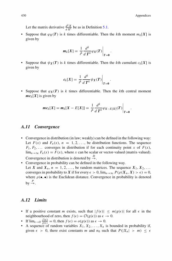
430 Appendices
Let the matrix derivative dk Y
d Xk be as in Definition 5.1.
• Suppose that ϕX(T ) is k times differentiable. Then the kth moment mk[X] isgiven by
mk[X] = 1
ikdk
d T kϕX(T )
∣
∣
∣
∣
T =0.
• Suppose that ψX(T ) is k times differentiable. Then the kth cumulant ck[X] isgiven by
ck[X] = 1
ikdk
d T kψX(T )
∣
∣
∣
∣
T =0.
• Suppose that ϕX(T ) is k times differentiable. Then the kth central momentmck[X] is given by
mck[X] = mk[X − E[X]] = 1
ikdk
d T kϕX−E[X](T )
∣
∣
∣
∣
T =0.
A.11 Convergence
• Convergence in distribution (in law; weakly) can be defined in the following way:Let F(x) and Fn(x), n = 1, 2, . . . , be distribution functions. The sequenceF1, F2, . . . converges in distribution if for each continuity point x of F(x),limn→∞ Fn(x) = F(x), where x can be scalar or vector-valued (matrix-valued).
Convergence in distribution is denoted byD→.
• Convergence in probability can be defined in the following way.Let X and Xn, n = 1, 2, . . . , be random matrices. The sequence X1,X2, . . .
converges in probability to X if for every ε > 0, limn→∞ P(ρ(Xn,X) > ε) = 0,where ρ(•, •) is the Euclidean distance. Convergence in probability is denoted
byP→.
A.12 Limits
• If a positive constant m exists, such that |f (ε)| ≤ m|g(ε)| for all ε in theneighbourhood of zero, then f (ε) = O(g(ε)) as ε → 0.
• If limε→0f (ε)g(ε)
= 0, then f (ε) = o(g(ε)) as ε → 0.• A sequence of random variables X1,X2, . . . , Xn is bounded in probability if,
given ε > 0, there exist constants m and n0 such that P(|Xn| > m) ≤ ε

Appendices 431
for all n ≥ n0. This is denoted by Xn = Op(1). If anXn = Op(1), thenXn = Op(a−1
n ). A sequence of random vectors x1, x2, . . . , xn is bounded inprobability if xi1, xi2, . . . , xin is bounded in probability for each i.
• If a sequence of random vectors x1, x2, . . . , xn converges to zero in probability,this is denoted by xn = o(1). If anxn = o(1), then xn = o(a−1
n ).
Note that the last two statements also hold for matrices, because any matrix can bevectorized.
A.13 Hermite Polynomials
Let X ∼ Np,n(μ,�,�) and let fX(Xo) be its density evaluated at Xo. Moreover,
let the derivative dkfX(Xo)
dXko
be defined in Lemma 5.1. Then
dkfX(Xo)
dXko
= (−1)kH k(Xo,μ,�,�)fX(Xo),
for the functions H k(Xo,μ,�,�), which are called generalized Hermite polyno-mials. If X ∼ Np,n(0, I , I ) or X ∼ Np(0, I ), we obtain polynomials which areusually termed Hermite polynomials.
Appendix B: Useful Technical Results
This appendix comprises several technical results which are frequently appliedthroughout Chaps. 1–8. In many of the suggested proofs, the reader is referred toKollo and von Rosen (2005), although the same results can often be found in othertexts.
B.1 Factorization and a Determinant Relation
The next theorem is often used when presenting canonical forms of linear andbilinear models.
Theorem B.1
(i) Let A: p × q be of rank q . Then there exist a non-singular matrix T and anorthogonal matrix � such that A′ = T (I q : 0)�.
(ii) Let V be p.d. Then there exist an orthogonal matrix of eigenvectors of V , �,and a diagonal matrix D of positive eigenvalues of V such that V = �D�′.

432 Appendices
Proof Statement (i) is a special case of the well-known QR-decomposition, e.g. seeGolub and Van Loan (2013) (see also Rao 1973, p. 20), and the proof of statement(ii) can be found in Kollo and von Rosen (2005, Corollary 1.2.39.1). �Theorem B.2 Let B = (b1, b2, . . . , bp) be an orthogonal basis with respect to apositive definite matrix W : p × p, i.e. b′
iWbj = 0, i �= j . Then
|W | = c−1p∏
k=1
|b′iWbi |, c = |B|2.
Proof The theorem is true because |W | = c−1|B ′WB| = c−1 ∏p
k=1 |b′iWbi |. �
B.2 Subspace Relations
Theorem B.3 Let A, B and C be matrices of proper sizes. Then
(i) if x ∈ C(A), then x = Aq for some q;(ii) if C(A) ⊆ C(B), then C(B)⊥ ⊆ C(A)⊥;
(iii) if C(A) ⊆ C(B), then C(B) = C(A) � C(B) ∩ C(A)⊥;(iv) (modular identity) C(A) ∩ (C(B) + C(A) ∩ C(C)) = C(A) ∩ C(B) + C(A) ∩
C(C);(v) C(A(A′Bo)o) = C(A) ∩ C(B);
(vi) C(A′(AA′Bo)o) = C(A′Bo)⊥ ∩ C(A′);(vii) C(A′) ⊆ C(A′Bo) is equivalent to C(A) ∩ C(B) = {0}.Proof All the proofs are given in Kollo and von Rosen (2005, Section 1.2). �Theorem B.4 For A and � of a proper size,
C�(A)⊥ = C(�Ao) = C((�−1A)o) = C(�−1A)⊥.
Proof By the definition of Ao, Ao′��−1A = 0, which verifies the equalities. �
Note that from this relation, it does not follow that C�(A) = C(�−1A), since inthis case we operate with different inner products on the left and right side.
B.3 Rank Relations
Theorem B.5 Let A and B be arbitrary matrices of proper sizes and let dim{•}denote the dimension of a vector space. Then
(i) r(A) = r(A′);(ii) dim{C(A) ∩ C(B)} = r(A(A′Bo)o) = r((Ao : Bo)o);

Appendices 433
(iii) r(A : B) = r(A) + r(B) − dim{C(A) ∩ C(B)};(iv) r(A′Bo) = r(A : B) − r(B).
Proof The proof of the theorem is presented in Kollo and von Rosen (2005,Section 1.2). �
B.4 Special Matrix Inverses
Theorem B.6 Let S be positive definite and suppose that V , W and H are of aproper size, with H−1 being supposed to exist. Moreover, suppose that ω is a scalarand put D = S−1V W and E = DS−1. Then
(i) (S + V HW ′)−1 = S−1 − S−1V (W ′S−1V + H−1)−1W ′S−1;(ii) (S + V HW ′)−1V H = S−1V (W ′S−1V + H−1)−1;
(iii) (S +ωV W ′)−1 = ∑2r+1k=0 (−1)kωkDkS−1 +ω2(r+1)Dr+1(S +V W ′)−1Er+1,
r = 1, 2, . . . ;(iv) (S + ωV W ′)−1 = ∑∞
k=0(−1)kωkDkS−1, provided that the sum exists.
Proof The proof of the first statement can be found in Kollo and von Rosen (2005,Proposition 1.3.6), and statement (ii) follows directly from statement (i) by applyinga few calculations. The expressions in statement (iii) and (iv) are presented in vonRosen (1995, Lemma 2.1). �
B.5 Matrix Relations Involving g-Inverses
Theorem B.7 Let C(K) ⊆ C(A′) and let S be p.d. Then
(i) K(A′S−1A)−A′S−1A = K;(ii) K(A′S−1A)−K ′ does not depend on the choice of g-inverse.
Proof Both statements follow since C(A′) = C(A′S−1A). �
B.6 Matrix Relations for Partitioned Matrices
Theorem B.8 Let
A =(
A11 A12
A21 A22
)
,
(
A11 A12
A21 A22
)
,
where the size of Aij corresponds to the size of Aij .

434 Appendices
(i) (A11)−1A12 = −A12A−122 ;
(ii) C(A12) ⊆ C(A11 − A12A−122 A21);
(iii) if A is p.d., then C(A12) ⊆ C(A11);(iv) if A is non-singular, then |A| = |A22||A11 − A12A
−122 A21|.
Proof For a proof, see, for example, Kollo and von Rosen (2005, Proposition 1.3.3).�
B.7 Inequalities
Theorem B.9
(i) Markov’s inequality. Let X be a non-negative integrable random variable anda > 0. Then
P(X ≥ a) ≤ E[X]/a.
(ii) If A − B is p.s.d., then trA ≥ trB .(iii) The tr-distance (see Sect. A.6). ||AQB − APB|| > ||CQD − CPD|| for all
P and Q if and only if BB ′ ⊗ A′A− DD′ ⊗C′C is p.d., where it is supposedthat the matrices are of proper sizes.
(iv) Let � and S be positive definite matrices of size p × p. Then
|�|− 12 n
e− 1
2 tr{�−1S} ≤ | 1nS|− 1
2 ne− 1
2 np,
and equality holds if and only if � = 1nS.
(v) For A (of full rank) and � (p.d.) of proper sizes (see Liu and Neudecker, 1997)
(A′A)−1A′�A(A′A)−1 ≤ (λ1 + λp)2
4λ1λ2(A′�−1A)−1,
where λp and λ1 are the smallest and largest eigenvalues of �, respectively.The ratio
μ1 = 4λ1λ2
(λ1 + λp)2
is the square of the first antieigenvalue of � (see Gustafson, 1972, 2012).
Proof For a proof of statement (i), see, for example, Gut (2013, Theorem 1.1,p. 120). Because of the linearity of the trace-function, statement (ii) is trivial.Statement (iii) follows by using the following equation:
tr{FGHH ′G′F ′} = vec′(FGH )vec(FGH ) = vec′(G)(HH ′ ⊗ F ′F )vec(G).

Appendices 435
The proof of statement (iv) can be found in Srivastava and Khatri (1979, Theo-rem 1.10.4) and for the proof of statement (v), the reader is referred to the referencesgiven in the statement. �
B.8 Linear Equations
Theorem B.10
(i) The matrix equation AXB = C in X. If C(C) ⊆ C(A) and C(C′) ⊆ C(B ′),the system of equations is consistent and has the following general solution:(C0 denotes any particular solution)
X = C0 + (A′)oZ1 + A′Z2Bo′
or
X = C0 + Z1Bo′ + (A′)oZ2B
′
or
X = C0 + (A′)oZ1B′ + A′Z2B
o′ + (A′)oZ3Bo′,
where Zi , i = 1, 2, 3, are arbitrary matrices of proper sizes.(ii) For the consistent equationAXB = C, the bilinear expressionKXL is unique
and equals KA−CB−L, if C(K ′) ⊆ C(A′) and C(L) ⊆ C(B). Note that onechoice of particular solution is C0 = A−CB−.
(iii) The homogeneous matrix equation AiXB i = 0, i = 1, 2, in X, has thefollowing general solution:
X = (A′2)
oZ1S′1 + (A′
1 : A′2)
oZ2S′2 + (A′
1)oZ3S
′3 + Z4S
′4
or
X = T 1Z1Bo′2 + T 2Z2(B1 : B)o
′ + T 3Z3Bo′1 + T 4Z4
or
X = T 3Z1S′1 + T 4Z2S
′1 + T 4Z3S
′2 + T 1Z4S
′3 + T 4Z5S
′3
+T 1Z6S′4 + T 2Z7S
′4 + T 3Z8S
′4 + T 4Z9S
′4,
where Zi , i = 1, . . . , 9, are arbitrary matrices of proper sizes, and Si and T i ,i = 1, . . . , 4, are any matrices satisfying
C(S1) = C(B1 : B2) ∩ C(B1)⊥, C(T 1) = C(A′
1 : A′2) ∩ C(A′
1)⊥,
C(S2) = C(B1) ∩ C(B2), C(T 2) = C(A′1) ∩ C(A′
2),
C(S3) = C(B1 : B2) ∩ C(B2)⊥, C(T 3) = C(A′
1 : A′2) ∩ C(A′
2)⊥,
C(S4) = C(B1 : B2)⊥, C(T 1) = C(A′
1 : A′2)
⊥.

436 Appendices
(iv) The homogeneous matrix equation A1X1B1 + A2X2B2 = 0 in X1 and X2has the following general solution:
X1 = −A−1 A2(A
′2A
o1 : (A′
2)o′)oZ3(B2(B
′1)
o)o′B2B
−1 + (A′
1)oZ1 + A′
1Z2Bo′1 ,
X2 = (A′2A
o1) : (A′
2)o)o
′Z3(B2(B
′1)
o)o′ + A′
2Ao1Z4B
o′2 + (A′
2)oZ5
or
X1 = −A−1 A2(A
′2A
o1)
o(A′2A
o1)
o′A′
2Z6(B2(B′1)
o)o′B2B
−1 + (A′
1)oZ1 + A′
1Z2Bo′1 ,
X2 = (A′2A
o1)
o′((A′
2Ao1)
o′A′
2)oZ5 + (A′
2Ao1)
o(A′2A
o1)
o′A′
2Z6(B2(B′1)
o)o′
+A′2A
o1Z4B
o′2 ,
where Zi , i = 1, . . . , 6, are arbitrary matrices.
Proof The proof of the statements can be found in Kollo and von Rosen (2005,Section 1.3.5). �
B.9 Results Involving Projectors
Next a few useful results for projectors are presented.
Theorem B.11 Let PA,V = A(A′V −1A)−AV −1. Then
(i) P A,V P A,V = P A,V , P A,V (I − P A,V ) = 0;(ii) tr{PA,V } = r(A);
(iii) C(PA,V ) = C(A), N (P A,V ) = C(V Ao);(iv) (projection theorem) C(PA,V B) = C(PA,V ) ∩ (N (P A,V ) + C(B));(v) I = P ′
Ao,V −1 + P A,V .
Proof The proofs of statements (i) and (ii) can be found in most lin-ear algebra books. The relations in statement (iii) are fairly trivial, sinceA(A′V −1A)−A′V −1A = A (e.g. see Kollo and von Rosen, 2005, Proposi-tion 1.2.2) and A(A′V −1A)−A′V −1V Ao = 0. The proof of statement (iv) ispresented in Kollo and von Rosen (2005, Theorem 1.2.16). Statement (v) followsfrom Theorem B.13. �
The following theorem constitutes a basis for handling linear models within atheoretical perspective and reflects a decomposition of the whole space into twosubspaces.
Theorem B.12 Let S be p.d., let A and B be arbitrary matrices of proper sizes andlet C be any matrix such that C(C) = C(A′) ∩ C(B). Then
A(A′SA)−A′ − ABo(Bo′A′SABo)−Bo′
A′
= A(A′SA)−C(C′(A′SA)−C)−C ′(A′SA)−A′.

Appendices 437
Proof Let S = I . The general case follows by changing A to S1/2A. If S = I , thestatement consists of three orthogonal projectors: PA, PABo and P A(A′A)−C . Theresult follows since
C(A) = C(ABo) � C(A) ∩ C(ABo)⊥ = C(ABo) � C(A(A′A)−C),
see Theorems B.3 (v) and B.11 (iv) in this appendix. �Theorem B.13 If S is p.d. and C(B) ⊆ C(A),
P A,S = P B,S + SP ′A,SBo(Bo′
SP ′A,SBo)−Bo′
P A,S.
A special case is
S−1 − Bo(Bo′SBo)−Bo′ = S−1B(B ′S−1B)−B ′S−1.
Proof The result follows from Theorem B.12. �
B.10 Properties of a Matrix Derivative
Theorem B.14 Let dk Y
d Xk be given by Definition 5.1. Then
(i) d Xd X
= Ipq , where X ∈ Rp×q ;
(ii) d cXd X
= cIpq , where X ∈ Rp×q ;
(iii) d A′vecXd X
= A;
(iv) d Y+Zd X
= d Yd X
+ d Zd X
.
(v) Let Z = Z(Y ) and Y = Y (X), then d Zd X
= d Yd X
d Zd Y
(chain rule);
(vi) d AXBd X
= B ⊗ A′;(vii) d AYB
d X= d Y
d X(B ⊗ A′);
(viii) d X′d X
= Kq,p, if X ∈ Rp×q ;
(ix) d YZd X
= d Yd X
(Z ⊗ I ) + d Zd X
(I ⊗ Y ′);(x) d tr{A′X}
d X= vecA;
(xi) d |X|d X
= |X|vec(X−1)′.(xii) If X: p × p is symmetric d X
d X= Ip2 + Kp,p − (Kp,p)d .
Proof The proofs of the statements can, for example, be found in Kollo and vonRosen (2005, Section 1.4.3, Table 1.4.2). �Theorem B.15 Let the derivative be given by Definition 8.4 and suppose that thematrices are conformable. If X and Y are functions of ω, then
(i) dkXYd ωk = ∑k
i=0
(
ki
)
diXd ωi
dk−iYd ωk−i , k ≥ 0.

438 Appendices
(ii) Let A and B be functionally independent of the scalar ω. Then
dkAXB
d ωk= A
dkX
d ωkB.
(iii) Let X be non-singular and a function of the scalar ω. Then
dkX−1
d ωk= −X−1 dkX
d ωkX−1 +
k−1∑
j=1
(−1)j+1k−1∑
i=1 j
i1−1∑
i=2 j−1
· · ·ij−1−1∑
i=j 1
(
ki1
)(
i1i2
) · · · (ij−1ij
)
×X−1 dij X
d ωijX−1 dij−1−ij X
d ωij−1−ijX−1 × · · · × X−1 di1−i2X
d ωi1−i2X−1 dk−i1X
d ωk−i1X−1,
i0 = k ≥ 1.
Proof The proofs of statements (i) and (iii) are presented in von Rosen (1995,Lemma 3.1) and statement (ii) follows from statement (i). �
B.11 Basic Moment Identities
Theorem B.16 Let E[X] = μ and D[X] = � ⊗ �. Then
(i) E[KXL] = KμL;(ii) D[KXL] = L′�L ⊗ K�K ′.
For moments and cumulants,
(iii) c1[X] = m1[X], c2[X] = D[X];(iv) mk[X] = E[vecX(vec′X)⊗k−1], m1[X] = E[vecX].Proof All proofs of the relations can be found in Kollo and von Rosen (2005,Section 2.1). �
B.12 Limit Theorems
The first theorem below is a multivariate version of some of the statements ofCramér’s theorem, which is also known as Slutsky’s theorem.
Theorem B.17 Let {Xn} and {Y n} be sequences of random matrices, not necessar-
ily independent, such that XnD→ X and Y n
P→ 0. Then, provided the operationsare well defined,
(i) Xn ⊗ Y nP→ 0;
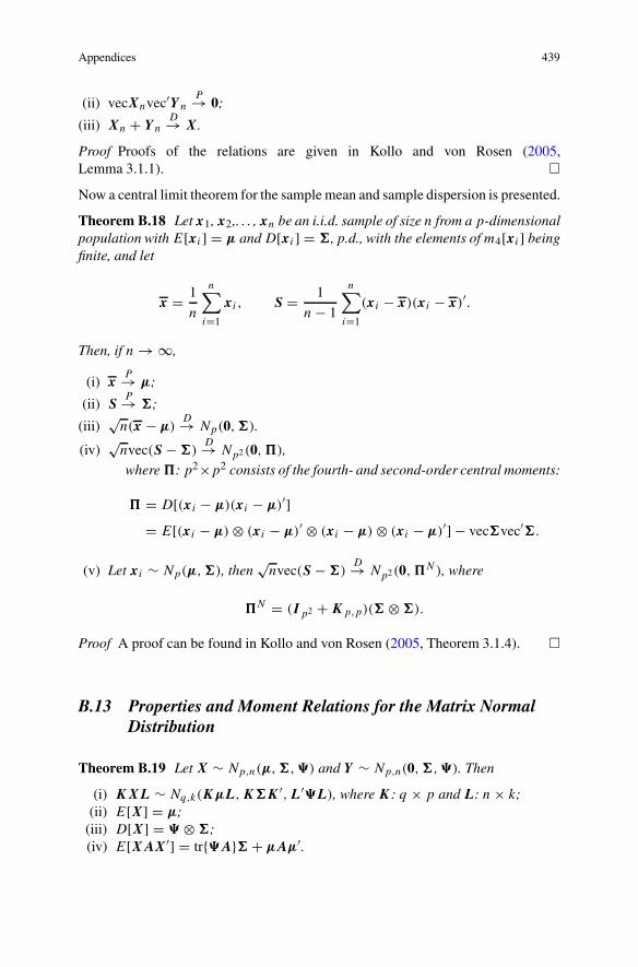
Appendices 439
(ii) vecXnvec′Y nP→ 0;
(iii) Xn + Y nD→ X.
Proof Proofs of the relations are given in Kollo and von Rosen (2005,Lemma 3.1.1). �Now a central limit theorem for the sample mean and sample dispersion is presented.
Theorem B.18 Let x1, x2,. . . , xn be an i.i.d. sample of size n from a p-dimensionalpopulation with E[xi ] = μ and D[xi ] = �, p.d., with the elements of m4[xi] beingfinite, and let
x = 1
n
n∑
i=1
xi , S = 1
n − 1
n∑
i=1
(xi − x)(xi − x)′.
Then, if n → ∞,
(i) xP→ μ;
(ii) SP→ �;
(iii)√
n(x − μ)D→ Np(0,�).
(iv)√
nvec(S − �)D→ Np2(0,),
where: p2×p2 consists of the fourth- and second-order central moments:
= D[(x i − μ)(xi − μ)′]= E[(xi − μ) ⊗ (xi − μ)′ ⊗ (xi − μ) ⊗ (xi − μ)′] − vec�vec′�.
(v) Let xi ∼ Np(μ,�), then√
nvec(S − �)D→ Np2(0,N), where
N = (Ip2 + Kp,p)(� ⊗ �).
Proof A proof can be found in Kollo and von Rosen (2005, Theorem 3.1.4). �
B.13 Properties and Moment Relations for the Matrix NormalDistribution
Theorem B.19 Let X ∼ Np,n(μ,�,�) and Y ∼ Np,n(0,�,�). Then
(i) KXL ∼ Nq,k(KμL,K�K ′,L′�L), where K: q × p and L: n × k;(ii) E[X] = μ;
(iii) D[X] = � ⊗ �;(iv) E[XAX′] = tr{�A}� + μAμ′.

440 Appendices
(v) Put H = (vec�vec′�)⊗2. Then
E[Y⊗4] = H + (Ip ⊗ Kp,p ⊗ Ip)H (In ⊗ Kn,n ⊗ I n)
+(Ip ⊗ Kp2,p)H (In ⊗ Kn,n2);
(vi) E[Y⊗2r ] = ∑2ri=2(Ip ⊗ Kpi−2,p ⊗ Ip2r−i )(vec�vec′� ⊗ E[Y⊗2(r−1)])
× (I n ⊗ Kn,ni−2 ⊗ I n2r−i ), r = 1, 2, 3, . . . ;(vii)
E[XAX′ ⊗ XBX′] = tr{�A}tr{�B}� ⊗ � + tr{�A�B ′}vec�vec′�
+tr{�A�B}Kp,p(� ⊗ �) + tr{�A}� ⊗ μBμ′ + vec(μB�A′μ′)vec′�
+Kp,p(μB�Aμ′ ⊗ � + � ⊗ μA�Bμ′)
+vec�vec′(μB ′�Aμ′) + tr{�B}μAμ′ ⊗ � + μAμ′ ⊗ μBμ′.
(viii) Let S = Y (I − P C ′)Y ′, where C is a matrix of a proper size. Then S andYP C ′ are independently distributed.
(ix) YPY ′ and YQY ′ are independently distributed if PQ = 0, where P and Q
are symmetric matrices of proper sizes.(x) YP and YQ are independently distributed if PQ′ = 0, where P and Q are
of proper sizes.(xi) YPY ′ and YQ are independently distributed if PQ = 0, where P and Q
are symmetric matrices of proper sizes.(xii) Let A be a matrix of a proper size. Then PA,X and (I − P A,)X are
independently distributed.(xiii) Let A and B be matrices of proper sizes. Then A′X and B ′X are indepen-
dently distributed if and only if C[AX,BX] = 0.
Proof For the proofs, see Section 2.2 in Kollo and von Rosen (2005), where theabove-presented results are obtained. �
B.14 Properties and Moment Relations for the WishartDistribution
Theorem B.20 Let W ∼ Wp(�, n), V ∼ Wp(I , n), where n > p. Then
(i) A′WA ∼ Wq(A′�A, n) for any matrix A of size p × q . In particular A =(I : 0) results in quadratic blocks along the diagonal of W also having aWishart distribution.
(ii) E[W ] = n�;(iii) D[W ] = n(I + Kp,p)� ⊗ �.

Appendices 441
(iv) Partition V as follows:
V =(
V 11 V 12
V 21 V 22
)
,
where V 11: r × r , V 12 = V ′21: r × (p − r) and V 22: (p − r) × (p − r).
Then V 12V−1/222 ∼ Nr,p−r (0, I , I ), and V 12V
−1/222 and V 22 ∼ Wp−r (I , n)
are independently distributed.(v) Let A: p × q . Then
A(A′W−1A)−A′ ∼ Wp(A(A′�−1A)−A′, n − p + r(A))
and
E[A(A′W−1A)−A′] = (n − p + r(A))A(A′�−1A)−A′.
(vi) Let X ∼ Np,n(0,�, I ) and P be any idempotent matrix of a proper size.Then
XPX′ ∼ Wp(�, r(P )).
(vii) A(A′W−1A)−A′ and W − A(A′W−1A)−A′ are independent.(viii) A(A′W−1A)−A′ and I − A(A′W−1A)−A′W−1 are independent.
(ix) E[A(A′WA)−A′W ] = A(A′�A)−A′�.
Proof Proofs of the above statements can be found in Kollo and von Rosen (2005,Section 2.4). Concerning statement (v), it is stressed that there exists a new proofwhich is fundamental. There always exists a matrix X ∼ Np,n(0,�, I ) such thatW = XX′. Then
A(A′W−1A)−A′ = P A,A(A′W−1A)−A′P ′A,
= P A,(W − WAo(Ao′WAo)−Ao′
W )P ′A, = P A,XPX′P ′
A,,
where P = I − X′Ao(Ao′WAo)−Ao′
X. The proof follows since A′�−1X andAo′
X are independently distributed and P is idempotent with rank r(P ) = n −r(Ao). �
B.15 Moments for the Inverse Wishart Distribution
In the following, the constants introduced in the next definition will frequently beapplied.

442 Appendices
Definition B.1
(i) c0;n,s = 1n−s−1 ;
(ii) c1;n,s,t = n−s−2(n−t−1)(n−s)(n−s−3)
;
(iii) c2;n,s,t = 1n−s−2c1;n,s,t ;
(iv) c3;n,s,t = 1(n−s−1)(n−t−1)
.
If s = t , then ci;n,s will be used instead of ci;n,s,s , i = 1, 2, 3.
Theorem B.21 Let W ∼ Wp(�, n) and let ci;n,s be defined in Definition B.1.Then,
(i) if n − p − 1 > 0,
E[W−1] = c0;n,p�−1;
(ii) if n − p − 3 > 0,
D[W−1] = c2;n,p(I + Kp,p)(�−1 ⊗ �−1) + (c1;n,p − c20;n,p)vec�−1vec′�−1;
(iii) if n − p − 3 > 0,
E[W−1 ⊗ W−1] = c2;n,p(vec�−1vec′�−1 + Kp,p(�−1 ⊗ �−1))
+ c1;n,p�−1 ⊗ �−1;
(iv) if n − p − 3 > 0,
E[tr{W−1}2] = 2c2;n,ptr{�−1�−1} + c1;n,ptr{�−1}2;
(v) if n − p − 3 > 0,
E[W−1W−1] = (c2;n,p + c1;n,p)�−1�−1 + c2;n,p�−1tr{�−1};
(vi) if n − p − 3 > 0,
E[tr{W−1W−1}] = (c2;n,p + c1;n,p)tr{�−1�−1} + c2;n,ptr{�−1}2.
(vii) Let
W =(
W 11 W 12
W 21 W 22
)
,
(
r × r r × p − r
p − r × r p − r × p − r
)
.
Then, if � = I and n − p + r − 1 > 0,
E[W 12W−122 W−1
22 W 21] = p − r
n − p + r − 1I r ,

Appendices 443
and if n − p + r − 3 > 0,
E[(vec(W 12W−122 W−1
22 W 21))⊗2] = tr{W−1
22 }2vecI r ⊗ vecI r
+ tr{W−122 W−1
22 }(I r2 + Kr,r ),
where tr{W−122 }2 and tr{W−1
22 W−122 } are given in statement (iv) and statement
(vi), respectively.(viii) E[A(A′W−1A)−A′W−1] = A(A′�−1A)−A′�−1.
Proof Proofs of statements (i)–(vi) can be obtained from Kollo and von Rosen(2005, Theorem 2.4.14). Concerning statement (vii), it is noted that W 12W
−1/222 ∼
Nr,p−r (0, I , I ) is independent of W 22 (see Appendix B, Theorem B.20 (iv)) andAppendix B, Theorem B.19 (v) together with statement (iv) and statement (vi) ofthis theorem establishes statement (vii). With regard to statement (viii), it is notedthat there exists a matrix A of full rank such that
A(A′W−1A)−A′W−1 = A(A′W−1A)−1A′W−1.
Moreover, there exist a non-singular matrix T and an orthogonal matrix � such thatA′ = T (I : 0)��1/2 = T �1�
1/2, and a V = ��−1/2W�−1/2�′ ∼ Wp(I , n).Then
E[A(A′W−1A)−A′W−1] = E[�1/2�′1(V
11)−1(V 11 : V 12)��−1/2]= �1/2�′
1�1�−1/2 = A(A′�−1A)−A′�−1,
since E[(V 11)−1V 12] = −E[V 12V−122 ] = 0. �
B.16 A Property and Moments for the Multivariate β Type IDistribution
Theorem B.22 Let F ∼ MβI(p,m, n), and let W 1 and W 2 be as in Sect. A.9.Then
(i) one choice of (W 1 + W 2)1/2 is a unique lower triangular matrix with positive
diagonal elements, let us say T , such that (W 1 + W 2) = T T ′ and F =T −1W 2(T
′)−1;(ii) E[F ] = m
m+nIp;
(iii) E[F−1] = m+n−p−1m−p−1 Ip.
Proof Statement (i) follows from a remark made after Theorem 2.4.8 in Kollo andvon Rosen (2005). Moreover, the proof of statement (ii) is given in Theorem 2.4.15

444 Appendices
(iii) in Kollo and von Rosen (2005), and statement (iii) follows from the proof ofTheorem 2.4.15 (i) in the same book. �
B.17 Special Moment Relations
Theorem B.23 Let Y ∼ Np,n(0,�,�) and Z ∼ Np,n(0, Ip, In). Then
(i) for the known constants q1 and q2, and the known symmetric matrices M andN ,
E[q1vec(Y )vec′(Y ) + q2tr{MYNY ′}vec(Y )vec′(Y )]= q1� ⊗ � + q2tr{N�}tr{M�}� ⊗ � + 2q2�N� ⊗ �M�;
(ii) E[Z′(ZZ′)−1Z] = pnIn.
Proof To verify statement (i), the statement is vectorized, i.e. instead of vecYvec′Y ,� ⊗ � and �N� ⊗ �M�,
vec(vecY vec′Y ) = vecY ⊗ vecY , vec(� ⊗ �), vec(�N� ⊗ �M�)
are used. Moreover, note that
tr{MYNY ′}(vecY )⊗2 = (vec′Ipn ⊗ I (pn)2)(N ⊗ I ⊗ I ⊗ M)(vecY )⊗4.
Thus, the fourth moments of a multivariate normally distributed variable are needed.From results in Kollo and von Rosen (2005, Corollary 2.2.7.4), it follows that
E[(vecY )⊗2] = vec(� ⊗ �),
E[(vecY )⊗4] = (I (pn)4 + Ipn ⊗ Kpn,pn ⊗ Ipn + Ipn ⊗ K(pn)2,pn)(vec(� ⊗ �))⊗2.
Utilizing these expressions, the statement follows from the following facts:
• (vec′Ipn ⊗ I (pn)2)(N ⊗ I ⊗ I ⊗ M)(vec(� ⊗ �))⊗2
= tr{N�}tr{M�}vec(� ⊗ �),• (vec′Ipn ⊗ I (pn)2)(N ⊗ I ⊗ I ⊗ M)(Ipn ⊗ Kpn,pn ⊗ Ipn)(vec(� ⊗ �))⊗2
= vec(�N� ⊗ �M�),• (vec′Ipn ⊗ I (pn)2)(N ⊗ I ⊗ I ⊗ M)(Ipn ⊗ K(pn)2,pn)(vec(� ⊗ �))⊗2
= vec(�N� ⊗ �M�).
To prove statement (ii), a different technique is used. Note that for all orthogonalmatrices, �,
�′E[Z′(ZZ′)−1Z]� = E[Z′(ZZ′)−1Z],

Appendices 445
since �′Z′(ZZ′)−1Z� = �′Z′(Z��′Z′)−1Z�, and the distribution of Z� equalsthe distribution of Z. Thus, E[Z′(ZZ′)−1Z] = cIn for some constant c. Now theconstant is determined by taking the trace, giving p = cn, and the statement isestablished. �Theorem B.24 LetW ∼ Wp(�, n) andA: p×q . The constants ci;n,s,t , i = 1, 2, 3,are given in Definition B.1. Then
E[A(A′WA)−A′ ⊗ W−1] = c1;n,r(A),pA(A′�A)−A′ ⊗ A(A′�A)−A′
+c2;n,r(A),p(vec(A(A′�A)−A′)vec′(A(A′�A)−A′)
+Kp,pA(A′�A)−A′ ⊗ A(A′�A)−A′)
+c3;n,r(A),pA(A′�A)−A′ ⊗ (�−1 − A(A′�A)−A′).
Proof Without any loss of generality, identify A by A, p × r(A) and use that A′ =T (I r(A) : 0)��−1/2 for some non-singular T and orthogonal �. Moreover, put
V = ��−1/2W�−1/2�′.
Then
E[A(A′WA)−A′ ⊗ W−1]
= (�−1/2�′)⊗2(E[(
V −111 00 0
)⊗2
] + E[(
V −111 00 0
)
⊗ H ])(��−1/2)⊗2,
where
H =(−V −1
11 V 12
I
)
(V 22 − V 21V−111 V 12)
−1(−V 21V−111 : I ).
Let V = UU ′, V 11 = U1U′1 and V 12 = U1U
′2, where
U = (U ′1 : U ′
2)′, U 1 : r(A) × n, U 2 : (p − r(A)) × n, U ∼ Np,n(0, I , I ).
It can be noted that, given U1, the matrix V 21V−111 is independent of V 2•1 = V 22 −
V 21V−111 V 12. Therefore, E[V −1
11 V 12V−12•1|U1] = 0, and
E[(
V −111 00 0
)
⊗ H ] = E[E[(
V −111 00 0
)
⊗ H |U1]]
= E[(
V −111 00 0
)
⊗(
E[V −111 V 12V
−12•1V 21V
−111 |U1] 0
0 E[V −12•1|U1]
)
].
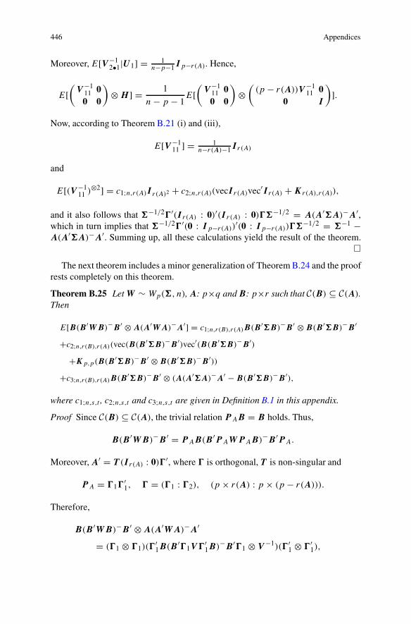
446 Appendices
Moreover, E[V −12•1|U1] = 1
n−p−1Ip−r(A). Hence,
E[(
V −111 00 0
)
⊗ H ] = 1
n − p − 1E[
(
V −111 00 0
)
⊗(
(p − r(A))V −111 0
0 I
)
].
Now, according to Theorem B.21 (i) and (iii),
E[V −111 ] = 1
n−r(A)−1I r(A)
and
E[(V −111 )⊗2] = c1;n,r(A)I r(A)2 + c2;n,r(A)(vecI r(A)vec′I r(A) + Kr(A),r(A)),
and it also follows that �−1/2�′(I r(A) : 0)′(I r(A) : 0)��−1/2 = A(A′�A)−A′,which in turn implies that �−1/2�′(0 : Ip−r(A))
′(0 : Ip−r(A))��−1/2 = �−1 −A(A′�A)−A′. Summing up, all these calculations yield the result of the theorem.
�The next theorem includes a minor generalization of Theorem B.24 and the proof
rests completely on this theorem.
Theorem B.25 LetW ∼ Wp(�, n),A: p×q andB: p×r such that C(B) ⊆ C(A).Then
E[B(B′WB)−B ′ ⊗ A(A′WA)−A′] = c1;n,r(B),r(A)B(B ′�B)−B ′ ⊗ B(B ′�B)−B ′
+c2;n,r(B),r(A)(vec(B(B ′�B)−B ′)vec′(B(B ′�B)−B′)
+Kp,p(B(B ′�B)−B ′ ⊗ B(B′�B)−B ′))
+c3;n,r(B),r(A)B(B′�B)−B ′ ⊗ (A(A′�A)−A′ − B(B ′�B)−B ′),
where c1;n,s,t , c2;n,s,t and c3;n,s,t are given in Definition B.1 in this appendix.
Proof Since C(B) ⊆ C(A), the trivial relation P AB = B holds. Thus,
B(B ′WB)−B ′ = P AB(B ′P AWP AB)−B ′P A.
Moreover, A′ = T (I r(A) : 0)�′, where � is orthogonal, T is non-singular and
P A = �1�′1, � = (�1 : �2), (p × r(A) : p × (p − r(A))).
Therefore,
B(B ′WB)−B ′ ⊗ A(A′WA)−A′
= (�1 ⊗ �1)(�′1B(B ′�1V �′
1B)−B ′�1 ⊗ V −1)(�′1 ⊗ �′
1),

Appendices 447
where V ∼ Wr(A)(�′1��1, n). Now the result follows from Theorem B.24, since
�1�′1B(B ′�1�
′1��1�
′1B)−B ′�1�
′1 = B(B ′�B)−B ′
and
�1(�′1��1)
−1�′1 = A(A′�A)−A′.
�Theorem B.26 Let S = X(I − P C ′)X′, where X ∼ Np,n(μ,�, I ), μ′ ∈ C(C′)and A: p × q . Moreover, let the constants ci;n,s,t , i = 1, 2, 3, be given inDefinition B.1 in this appendix. Then
(i) E[S−1A(A′S−1A)−A′S−1]= c0;n−r(C),p�−1 − c0;n−r(C),p−r(A)A
o(Ao′�Ao)−Ao′
;
(ii) E[A(A′S−1A)−A′S−1�S−1A(A′S−1A)−A′]= n−r(C)−1
n−r(C)−p+r(A)−1A(A′�−1A)−A′;
(iii) E[S−1A(A′S−1A)−A′S−1�S−1A(A′S−1A)−A′S−1] = ((p + 1)c2;n,p +c1;n,p)�−1 + ((p− r(A)+1)(c2;n,p−r(A) −2c2;n,r(A),p−r(A))+c1;n,p−r(A) −c1;n,r(A),p−r(A)) × Ao(Ao′
�Ao)−Ao′.
Proof Concerning statement (i), it is noted that
S−1A(A′S−1A)−A′S−1 = S−1 − Ao(Ao′SAo)−Ao′
and, according to Theorem B.21 (i),
E[S−1] = c0,n−r(C),p�−1,
E[Ao(Ao′SAo)−Ao′ ] = c0,n−r(C),p−r(A)A
o(Ao′�Ao)−Ao′
,
which establishes statement (i).Concerning statement (ii), suppose, without any loss of generality, that A is of
full rank and factor A as A′ = T (I : 0)��1/2, where T is non-singular and �
orthogonal. Utilizing Theorem B.21 (vii) establishes the result.The expression in statement (iii) is more complicated to handle than statement
(ii). Note that
E[S−1A(A′S−1A)−A′S−1�S−1A(A′S−1A)−A′S−1]= E[(S−1 − Ao(Ao′
SAo)−1Ao′)�(S−1 − Ao(Ao′
SAo)−1Ao′)]
and, therefore, the following three types of moment calculations are needed:E[S−1�S−1], E[Ao(Ao′
SAo)−1Ao′�Ao(Ao′
SAo)−1Ao′ ] and E[S−1�Ao
(Ao′SAo)−1Ao′ ].

448 Appendices
Since �−1/2S�−1/2 ∼ Wp(I , n), according to Theorem B.21 (v),
E[S−1�S−1] = �−1/2E[(�−1/2S�−1/2)−1(�−1/2S�−1/2)−1]�−1/2
= (c2;n,p + c1;n,p)�−1 + c2;n,pp�−1. (B.1)
Similarly, since (Ao′�Ao)−1/2Ao′
SAo′(Ao′
�Ao)−1/2 ∼ Wp−r(A)(I , n), applyingTheorem B.21 (v) once again yields
E[Ao(Ao′SAo)−1Ao′
�Ao(Ao′SAo)−1Ao′ ]
= (c2;n,p−r(A) + c1;n,p−r(A) + c2;n,p−r(A)(p − r(A)))Ao(Ao′�Ao)−1Ao′
.(B.2)
Concerning the third type of moment expressions, it is convenient to rely onTheorem B.24. Post-multiplying the statement of Theorem B.24 by vec� andreplacing A by Ao: p × p − r(A) leads to
E[Ao(Ao′WAo)−Ao′ ⊗ W−1]vec� = vec(E[W−1�Ao(Ao′
WAo)−Ao′ ])= c1;n,r(A),p−r(A)vec(Ao(Ao′
�Ao)−Ao′)
+c2;n,r(A),p−r(A)((p − r(A))vec(Ao(Ao′�Ao)−Ao′
) + vec(Ao(Ao′�Ao)−Ao′
)).
Thus, E[W−1�Ao(Ao′WAo)−Ao′ ] = E[Ao(Ao′
WAo)−Ao′�W−1] and
E[W−1�Ao(Ao′WAo)−Ao′ ]
= (c1;n,r(A),p−r(A) + c2;n,r(A),p−r(A)(p − r(A) + 1))Ao(Ao′�Ao)−Ao′
). (B.3)
Summing (B.1) and (B.2), and subtracting two times (B.3) establish statement (iii).�
Problems
1 For any A and C such that C(C′) ⊆ C(A′) and V , p.d., of proper sizes, show thatC(A′V A)−A′V A = C.
2 Show that AX−C does not depend on the choice of g-inverse if and only ifC(A′) ⊆ C(X′) and C(C) ⊆ C(X) hold.
3 Suppose that all the given operations are well defined. Show that
AA′(AA′ + BB ′)−BB ′ = BB ′(AA′ + BB ′)−AA′.

Appendices 449
4 Suppose that there is a simple matrix block structure whose inverse exists andwhich is as follows:
(
A B
−B A
)
.
Derive its inverse.Suppose now that a minor extension of the above block structure is available,
providing the following structure:
⎛
⎜
⎜
⎝
A B C D
−B A −D C
−C D A −B
−D −C B A
⎞
⎟
⎟
⎠
.
Derive the inverse matrix of the given block structure. Try to find out why thesestructures are connected to complex numbers and quaternions.
5 Let A and B be of proper sizes. Show that C(AA′Bo) ∩ C(B) = {0}.6 Show that C(A1 ⊗ B1) is orthogonal to C(A2 ⊗ B2) if and only if C(A1) isorthogonal to C(A2) or C(B1) is orthogonal to C(B2).
7 A subspace C(M) is A-invariant if C(AM) ⊆ C(M). Show that C(M) is A-invariant if and only if C(M)⊥ is A′-invariant.
8 Let A: p × q , B: q × r , C: r × s and D: s × p. Show that tr{ABCD} =(vec′(C′) ⊗ vec′A)(I r ⊗ Ks,q ⊗ Ip)vecB ⊗ vecD′).
9 Let A: r × s, B: s × t , C: m × n and D: n × p. Show that
AB ⊗ CD = (I rm ⊗ vec′D′)(I r ⊗ vecC′vec′B ′ ⊗ Ip)(vecA′ ⊗ Ipt ).
10 Show that x⊗3 = (Kp,p ⊗ Ip)Kp2,px⊗3, where x is a vector of size p.
11 Interpret the matrices 12 (Ip2 + Kp,p), 1
2 (Ip2 − Kp,p) and (Kp,p)d .
12 Let A, B and T be upper triangular matrices and put U = AT B. Derive theJacobian for the transformation from T to U .
13 Let T be a Toeplitz matrix. Use a matrix derivative dd T
and study dTd T
.
14 Let X ∼ Np,n(μ,�,�). Derive E[X⊗4].15 Let X ∼ Np,n(0,�,�), and let A, B and C be fixed matrices of proper sizes.Derive E[XAX′ ⊗ XBX′ ⊗ XCX′].16 For a matrix normal distribution, show that all the cumulants of an order > 2equal 0. Let U ∼ Wp(Ip, n) and suppose that p > n. Because of Wishartness,U = YY ′, Y = (Y ′
1 : Y ′2)
′, Y ∼ Np,n(0, Ip, In) and Y 1 ∼ Nn,n(0, In, In); it is

450 Appendices
assumed that r(Y 1) = n. Derive the Moore-Penrose inverse of U as a function ofY 1 and Y 2.
17 Let X1 ∼ Np,n(μ1,�1,�1) and X2 ∼ Np,n(μ2,�2,�2), and let Z have amixture distribution defined through the density
fZ(X) = γfX1(X) + (1 − γ )γfX2(X), 0 < γ < 1.
Derive D[Z] and E[Z⊗2].18 Let W 1 ∼ Wp(�1, n) and W 2 ∼ Wp(�1,m). Show that W 1 + W 2 ∼Wp(�, n + m).
19 Let W ∼ Wp(�, n). Derive E[tr{W−1}W ].20 Let W ∼ Wp(�, n). Derive the asymptotic normal distribution for W−1 whenn → ∞.
Appendix C: Test Statistics
C.1 Distribution of Test Statistics
The test statistics presented and applied in Chap. 7 are all functions of Wishart-distributed quadratic forms and, in principle, the distributions of the test statistics arederived from assumptions about the MANOVA model as it is discussed in Chap. 7.Let
X = μC + E, E ∼ Np,n(0,�, I ),
where μ: p × k is the unknown parameter describing the mean, �: p × p is theunknown positive definite dispersion matrix and C: k × n is a known between-individuals design matrix. Moreover, suppose that the restrictions which are to betested are given by
H0 : μG = 0,
where G is a known matrix. The hypothesis H0 is tested against an alternativehypothesis, H1, which states that μ is unrestricted. Then the likelihood ratio test
statistic in this book is equivalent to U− 1
2 n
p,m,f , where
Up,m,f = |n�1||n�0|
, (C.1)
with f = n − r(C), m = dim{C(G) ∩ C(C)} and

Appendices 451
n�1 = X(I − P C ′)X′, n�0 = X(I − P C ′Go)X′.
Let N be any matrix satisfying C(N) = C(G) ∩ C(C), which implies (see the proofof Theorem B.12 in Appendix B) that
C(C′Go)⊥ = C(C′)⊥ � C(C′) ∩ C(C′Go)⊥ = C(C′)⊥ � C(C′(CC′)−N).
Then
�0 = �1 + �2,
where n�2 = XP C ′(CC ′)−NX′ and
Up,m,f = |n�1||n�1 + μN(N ′(CC′)−N)−1N ′μ′| ,
where μN = XC′(CC ′)−N . It also follows that D[μN ] = N ′(CC′)−N and, if thenull hypothesis is true, μN should be “small”. Moreover, the statistic Up,m,f < 1if and only if C(C) ∩ C(G) �= {0}. Often it is assumed that C(G) ⊆ C(C) (thetestability condition), but this is not necessary. The statistic Up,m,f makes senseand is understandable.
Concerning the distribution of Up,m,f , n�1 ∼ Wp(�, f ), under H0 it followsthat n�2 ∼ Wp(�,m). Hence, under H0,
Up,m,f = |W 1||W 1 + W 2| = |(W 1 + W 2)
−1/2W 2(W 1 + W 2)−1/2|, (C.2)
where W 1 ∼ Wp(�, f ) and W 2 ∼ Wp(�,m), with W 1 and W 2 independentlydistributed. The test statistic is invariant with respect to non-singular transformationsof X and, therefore, � may be replaced by I ; i.e. (C.2) does not depend on �.Thus, Up,m,f is the determinant of a multivariate β-distribution of type I (seeSect. A.9 in Appendix A). The following lemma presents a Bartlett decompositionfor F ∼ MβI (p,m, n) which provides the fundament for studying the distributionof Up,m,f , as well as the distribution of the likelihood ratio test statistic for testingH0: μG = 0.
Lemma C.1 Let F ∼ MβI (p,m, n) and F = T T ′, where T is a lower triangularmatrix with positive diagonal elements. Then T11, T22, . . . , Tpp are all independentand
T 2ii ∼ β(m + 1 − i, n), i = 1, 2, . . . , p.
Proof Since F is positive definite, a lower triangular matrix T always exists suchthat F = T T ′. The density for F is given in Appendix A, Sect. A.10, and combiningthis expression with the factorization F = T T ′, together with the Jacobian for the

452 Appendices
variable transformation (see Kollo and von Rosen, 2005, Theorem 1.4.18), yields
c(p, n)c(p,m)
c(p, n + m)|T T ′|
m−p−12 |I − T T ′|
n−p−12 2p
p∏
i=1
Tp−i+1ii
= 2p c(p, n)c(p,m)
c(p, n + m)
p∏
i=1
T m−iii |I − T T ′|
n−p−12 . (C.3)
Now it is shown that T 211 is beta-distributed. Partition T as follows:
T =(
T11 0t21 T 22
)
.
Thus,
|I − T T ′| = (1 − T 211)(1 − v′v)|I − T 22T
′22|,
where
v = (I − T 22T′22)
−1/2t21(1 − T 211)
−1/2.
In the next equation, a change of variables takes place, i.e. T11, t21,T 22 →T11, v,T 22, and the corresponding Jacobian equals
|J (t21, T11, T 22 → v, T11, T 22)|+ = |J (t21 → v)|+ = (1 − T 211)
p−12 |I − T 22T
′22|
12 ,
where the last equality was obtained by the definition of a Jacobian (e.g. see Kolloand von Rosen, 2005). Thus, the joint density of T11, v and T 22 equals
2p c(p, n)c(p,m)
c(p, n + m)T m−1
11 (1 − T 211)
n−p−12
p∏
i=2
T m−iii
×|I − T 22T′22|
n−p−12 (1 − v′v)
n−p−12 (1 − T 2
11)p−1
2 |I − T 22T′22|
12
= 2p c(p, n)c(p,m)
c(p, n + m)(T 2
11)m−1
2 (1 − T 211)
n2 −1
×p∏
i=2
T m−iii |I − T 22T
′22|
n−p2 (1 − v′v)
n−p−12 .
Hence, T11 is independent of both T 22 and v. Moreover, making another transfor-mation, T11 → T 2
11, and applying its Jacobian yield that T 211 ∼ β(m, n) distributed.

Appendices 453
To obtain the distribution for T22, T33,. . . Tpp, one uses the fact that T 22 isindependent of T11 and v, and its density is proportional to
p∏
i=2
T m−iii |I − T 22T
′22|
n−p2 .
This density function has the same form as the one given in (C.3), and by repeatingarguments and using the fact that the size of T22 equals (p − 1)× (p − 1), it followsthat T22 ∼ β(m − 1, n) distributed. Continuing in the same fashion with Tii , i =3, 4, . . . , p, establishes the lemma. �Now, applying Lemma C.1 yields Theorem C.1.
Theorem C.1 Let W 1 ∼ Wp(�, f ), p ≤ f , W 2 ∼ Wp(�,m), p ≤ m, and letUp,m,f be given by (C.2). Then
Up,m,f =p∏
i=1
βi,
where βi is independent of βj , i �= j , and
βi ∼ β(m + 1 − i, f ).
From general asymptotic likelihood theory, it follows that
− 2 ln Up,m,fa∼χ2
pm, (C.4)
since BG = 0 implies that pm restrictions have been introduced on the parameterspace. It is now shown that this result can be improved via some expansion (the so-called Bartlett correction), i.e. the convergence can be made faster than O(n−1/2),which is the usual speed of the central limit theorem, which was applied whenshowing (C.4).
Since 0 ≤ Up,m,f ≤ 1, the statistic has compact support and, therefore, themoments determine the distribution. From Theorem C.1 it follows that the kthmoment of Up,m,f is known. Thus, since
E[Ukp,m,f ] = E[ek ln Up,m,f ],
the moment-generating function for −2 ln Up,m,f is available. For details about howto utilize this result, see Srivastava and Khatri (1979) or Anderson (2003).
In the next theorem some special cases of (C.2) are presented where exactdistributional results exist, and which can be shown to hold via moment calculations.Finding some exact special cases should be possible, because if, for example, p = 1,

454 Appendices
we are working within univariate analysis of variance, where exact F -tests are usedfor testing H0.
Theorem C.2 Let Up,m,f be given by (C.2) and let Fa,b denote the F -distributionwith parameters a and b (see Sect. A.9 in Appendix A). Then
(i) Up,m,f ∼ Um,p,f +m−p,
(ii) T1 = (f−1)m
(1 − U1/22,m,f )/U
1/22,m,f ∼ F2m,2(f−1),
(iii) T2 = fm
(1 − U1,m,f )/U1,m,f ∼ Fm,f .��
In fact, the above theorem covers quite a large number of testing situations,since after transformation and conditioning, it is often the case that p = 1 orp = 2. Concerning the distribution of the general case, the reader is referred toSrivastava and Khatri (1979) or Anderson (2003). The main problem is that it isdifficult to invert the moment-generating function and therefore one has to relyon approximations. Since the moment-generating function is a function of gammafunctions, the idea is to approximate these functions appropriately, i.e. as functionsof the moment-generating function for a chi-square distributed variable. After agreat deal of bookkeeping of terms in expansions, this provides the next importanttheorem.
Theorem C.3 Let Up,m,f be given by (C.2). Then
(i)
P {−(f − 12 (p − m + 1)) ln Up,m,f ≤ z} a∼P {χ2
pm ≤ z}+ c1(1 − c1)(P {χ2
pm+4 ≤ z} − P {χ2pm ≤ z}) + c2(P {χ2
pm+8 ≤ z} − P {χ2pm ≤ z})
+ O(n−6),
where
c1 = pm(p2 + m2 − 5)
48(f − 12 (p − m + 1))2
,
c2 = 12c2
1 + pm(3p4 + 3m4 + 10p2m2 − 50(p2 + m2) + 159)
1920(f − 12 (p − m + 1))4
.
(ii) Let λ = U− 1
2 n
p,m,f be the likelihood ratio statistics for testing H0:μG = 0 againstH1: μ unrestricted. Then
P { 2n(f − 1
2 (p − m + 1)) ln λ ≤ z} = P {−(f − 12 (p − m + 1)) ln Up,m,f ≤ z}.

Appendices 455
Proof A proof of statement (i) is given in Srivastava and Khatri (1979, Sec-tion 6.3.7) and Anderson (2003, Theorem 8.5.2), �
Note that c1 = O(n−2) and c2 = O(n−4). However, c1 = O(p) and c2 = O(p2)
and, therefore, for large p > n, the approximation given above will not behave well;i.e. if p/n → 1 when (p, n) → (∞,∞), then c1 and c2 turn to ∞.
Corollary C.1 Let Up,m,f be given by (C.2). Then
(i)
P {−(f − 12 (p − m + 1)) ln Up,m,f ≤ z} a∼ P {χ2
pm ≤ z} + O(n−2);
(ii)
P {−(f − 12 (p − m + 1)) ln Up,m,f ≤ z} a∼ P {χ2
pm ≤ z}+ c1(1 − c1)(P {χ2
pm+4 ≤ z} − P {χ2pm ≤ z}) + O(n−4).
��
References
Anderson, T. W. (2003). An introduction to multivariate statistical analysis. Wiley series inprobability and statistics (3rd ed.). Hoboken: Wiley-Interscience, Wiley.
Golub, G. H., & Van Loan, C. F. (2013). Matrix computations. Johns Hopkins studies in themathematical sciences (4th ed.). Baltimore: Johns Hopkins University Press.
Gustafson, K. (1972). Antieigenvalue inequalities in operator theory. In O. Shisha (Ed.), Inequali-ties III (pp. 115–119). New York: Academic.
Gustafson, K. (2012). Antieigenvalue analysis. With applications to numerical analysis, wavelets,statistics, quantum mechanics, finance and optimization. Hackensack: World Scientific Pub-lishing.
Gut, A. (2013). Probability: A graduate course. Springer texts in statistics (2nd ed.). New York:Springer.
Kollo, T., & von Rosen, D. (2005). Advanced multivariate statistics with matrices. Mathematicsand its applications (Vol. 579). Dordrecht: Springer.
Liu, S., & Neudecker, H. (1997). Kantorovich and Cauchy-Schwarz inequalities involving positivesemidefinite matrices, and efficiency comparisons for a singular linear model. Linear Algebraand Its Applications, 259, 209–221.
Rao, C. R. (1973). Linear statistical inference and its applications. Wiley series in probability andmathematical statistics (2nd ed.). New York: Wiley.
Srivastava, M. S., & Khatri, C. G. (1979). An introduction to multivariate statistics. New York:North-Holland.
von Rosen, D. (1995). Influential observations in multivariate linear models. Scandinavian Journalof Statistics, 22, 207–222.

Subject Index
Note that BRM , EBRM3B and EBRM3
W appear before the key words which aregiven in alphabetical order. There will be no references given to Appendix A orAppendix B, and only a few references are given to Appendix C.
BRM
asymptotically equivalentB , B , 102�, � , 103
convergence in distribution�, 104
convergence in probabilityB , 103�, 104
Edgeworth-type expansionB , 187, 188residual, R11, 234residual, R12, 235residual, R2, 236
hypothesis testingF 1BG1 = F 2�G2, 350F 1BG1 = 0 given F 2BG2 = 0,
C(F ′1) ⊆ C(F ′
2), 299, 304F 2BG2 = 0 given F 1BG1 = 0,
C(F ′1) ⊆ C(F ′
2), C(G2) ⊆ C(G1),309, 310
F 2BG2 = 0 given F 1BG1 = 0,C(F ′
1) ⊆ C(F ′2),
C(G2) ⊆ C(G1), 306F iBGi = 0, i=1,2, C(F ′
1) ⊆ C(F ′2),
312, 314F iBGi = 0, i=1,2, C(F ′
1) ⊆ C(F ′2),
C(G2) ⊆ C(G1), 317, 321maximum likelihood estimators
B , � when F 1BG1 = F 2�G2, 352
B, known dispersion, 52B, unknown dispersion, 74�, 74
moments of estimatorsD[B], 105D[�], 111D[E[X]], 107E[B], 105E[B⊗4], 108E[�], 111
moments of trace test statisticT3, 328T4, 334T51, 341T52, 340
perturbationB, case (i), 386B, case (ii), 380, 381B, case (iii), 375, 376�, case (iii), 389–391within-individual, 388
residualsR1, definition, 225R1, mean shift test, 252R1, moments, 227R2, definition, 225R2, moments, 227R11, definition, 225R11, mean shift test, 247R11, moments, 227
© Springer International Publishing AG, part of Springer Nature 2018D. von Rosen, Bilinear Regression Analysis, Lecture Notes in Statistics 220,https://doi.org/10.1007/978-3-319-78784-8
457
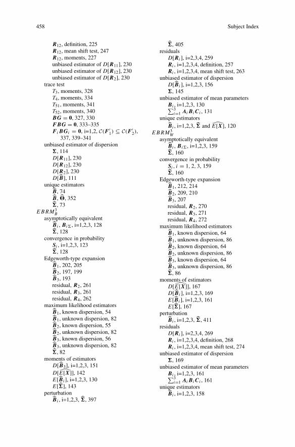
458 Subject Index
R12, definition, 225R12, mean shift test, 247R12, moments, 227unbiased estimator of D[R11], 230unbiased estimator of D[R12], 230unbiased estimator of D[R2], 230
trace testT3, moments, 328T4, moments, 334T51, moments, 341T52, moments, 340BG = 0, 327, 330FBG = 0, 333–335F iBGi = 0, i=1,2, C(F ′
1) ⊆ C(F ′2),
337, 339–341unbiased estimator of dispersion
�, 114D[R11], 230D[R12], 230D[R2], 230D[B], 111
unique estimatorsB , 74B , �, 352�, 73
EBRM3B
asymptotically equivalentB i , Bi , i=1,2,3, 128�, 128
convergence in probabilitySi , i=1,2,3, 123�, 128
Edgeworth-type expansionB1, 202, 205B2, 197, 199B3, 193residual, R2, 261residual, R3, 261residual, R4, 262
maximum likelihood estimatorsB1, known dispersion, 54B1, unknown dispersion, 82B2, known dispersion, 55B2, unknown dispersion, 82B3, known dispersion, 56B3, unknown dispersion, 82�, 82
moments of estimatorsD[B3], i=1,2,3, 151D[E[X]], 142E[B i], i=1,2,3, 130E[�], 143
perturbationB i , i=1,2,3, �, 397
�, 405residuals
D[Ri ], i=2,3,4, 259Ri , i=1,2,3,4, definition, 257Ri , i=1,2,3,4, mean shift test, 263
unbiased estimator of dispersionD[B i ], i=1,2,3, 156�, 145
unbiased estimator of mean parametersBi , i=1,2,3, 130∑3
i=1 AiB iCi , 131unique estimators
Bi , i=1,2,3, � and E[X], 120EBRM3
W
asymptotically equivalentBi , B i , i=1,2,3, 159�, 160
convergence in probabilitySi , i = 1, 2, 3, 159�, 160
Edgeworth-type expansionB1, 212, 214B2, 209, 210B3, 207residual, R2, 270residual, R3, 271residual, R4, 272
maximum likelihood estimatorsB1, known dispersion, 64B1, unknown dispersion, 86B2, known dispersion, 64B2, unknown dispersion, 86B3, known dispersion, 64B3, unknown dispersion, 86�, 86
moments of estimatorsD[E[X]], 167D[B i ], i=1,2,3, 169E[Bi ], i=1,2,3, 161E[�], 167
perturbationBi , i=1,2,3, �, 411
residualsD[Ri ], i=2,3,4, 269Ri , i=1,2,3,4, definition, 268Ri , i=1,2,3,4, mean shift test, 274
unbiased estimator of dispersion�, 169
unbiased estimator of mean parametersBi , i=1,2,3, 161∑3
i=1 AiB iCi , 161unique estimators
Bi , i=1,2,3, 158

Subject Index 459
� and E[X], 158
asymptotically equivalentBRM
B , B , 102�, � , 103
EBRM3B
B i , Bi , i=1,2,3, 128�, 128
EBRM3W
B i , Bi , i=1,2,3, 159�, 160
Bartlett correction, 453Bartlett decomposition, 451between-individuals design matrix, 11, 12, 14,
51between-individuals subspace, 63, 290, 342bilinear model, 2, 13bilinear regression model, 13, 39bilinear restrictions, 60, 93, 284BLUE, 52Bonferroni correction, 314
Cayley-Hamilton theorem, 100characteristic function, 177, 178chi-square approximation, 330, 335, 341, 342convergence in distribution
BRMB , 103�, 104
BRM
S, 101convergence in probability
BRMB , 103�, 104S, 185
EBRM3B
Si , i=1,2,3, 123�, 128
EBRM3W
Si , i=1,2,3, 159�, 160
BRMS, 101curved exponential family, 13, 74, 101
definition of dispersion, 286definition of models
BRM , 50BRM /growth curve model/GMANOVA,
13EBRMm
B , 53EBRMm
W , 62GMANOVA+MANOVA, 91MANOVA, 11
definition of multivariate cumulants, 178definition of perturbations
multivariate linear modelCase (i), Case (ii), Case (iii), 373
univariate linear modelCase (i), Case (ii), Case (iii), 366
definition of residualsBRM
R1, R2, R11, R12, 225EBRM3
B
Ri , i=1,2,3,4, 257EBRM3
W
Ri , i=1,2,3,4, 268
Edgeworth-type expansion, 178, 179, 181, 259BRM
B, 187, 188residual, R11, 234residual, R12, 235residual, R2, 236
EBRM3B
B1, 202, 205B2, 197, 199B3, 193residual, R2, 261residual, R3, 261residual, R4, 262
EBRM3W
B1, 212, 214B2, 209, 210B3, 207residual, R2, 270residual, R3, 271residual, R4, 272
estimability conditionsBRM , 104EBRM3
B , 120EBRM3
W , 158exponential family, 3, 6, 11, 13, 74, 101extended growth curve model, 15
Fourier transform, 178inverse, 180, 182

460 Subject Index
Gauss-Markov model, 6, 39, 41, 46singular, 9, 39, 67strongly singular, 46, 67weakly singular, 46, 67
GMANOVA, 13, 30GMANOVA+MANOVA, 93, 172, 215, 218,
276, 355, 413growth curve model, 13, 14, 30
half-invariants, 217Hermite polynomial, 180hypothesis testing
BRM , 286F 1BG1 = F 2�G2, 350F 1BG1 = 0 given F 2BG2 = 0,
C(F ′1) ⊆ C(F ′
2), 299, 304F 2BG2 = 0 given F 1BG1 = 0,
C(F ′1) ⊆ C(F ′
2), C(G2) ⊆ C(G1),306, 309, 310
F iBGi = 0, i=1,2, C(F ′1) ⊆ C(F ′
2),312, 314
F iBGi = 0, i=1,2, C(F ′1) ⊆ C(F ′
2),C(G2) ⊆ C(G1), 317, 321
EBRM3B against a BRM , 343, 348
MANOVABG = 0, 281, 284
influence analysisBRM , 373EBRM3
B , 393EBRM3
W , 407influence curve, 416influential observations, 4, 67, 221, 363inner product, 6, 46, 52, 75, 76, 105, 269inverse Fourier transform, 180, 182
Kotz-type distribution, 187, 188, 194, 208, 216Kroneckerian power, 108
least squares, 2, 4, 238, 242, 243likelihood ratio test versus trace test, 342linear equations, 7, 281, 287, 299, 312, 337,
351
MANOVA, 11, 49, 74, 104, 222, 224, 229,252, 281, 283, 284
Markov’s inequality, 103, 125, 126masking, 249, 370, 372, 415matrix derivative, 178, 373, 377, 394
maximum likelihood estimatorsBRM
B, 74B, � when F 1BG1 = F 2�G2, 352B, known dispersion, 52�, 74
EBRM3B
B1, known dispersion, 54B1, unknown dispersion, 82B2, known dispersion, 55B2, unknown dispersion, 82B3, known dispersion, 56B3, unknown dispersion, 82�, 82
EBRM3W
B1, known dispersion, 64B1, unknown dispersion, 86B2, known dispersion, 64B2, unknown dispersion, 86B3, known dispersion, 64B3, unknown dispersion, 86�, 86
MANOVA, 74mean shift test for residuals
BRM , 237R1, 252R11, 247R12, 247
EBRM3B
Ri , i=1,2,3,4, 263EBRM3
W
Ri , i=1,2,3,4, 274MANOVA, 222
moments of estimatorsBRM
D[B], 105D[�], 111D[E[X]], 107E[B], 105E[B⊗4], 108E[�], 111B, 109�, 230
EBRM3B
D[B i ], i=1,2,3, 151D[E[X]], 142E[Bi ], i=1,2,3, 130E[�], 143
EBRM3W
D[B i ], i = 1, 2, 3, 169D[E[X]], 167E[Bi ], i=1,2,3, 161E[�], 167

Subject Index 461
moments of residualsBRM
R1,R11,R12,R2, 227, 232EBRM3
B
D[Ri ], i=2,3,4, 259EBRM3
W
D[Ri ], i=2,3,4, 269moments of trace test statistic
BRM
T3, 328T4, 334T51, 341T52, 340
monomials, 108multivariate cumulant, 179multivariate linear model, 11, 39, 49, 99, 221,
281, 373
non-random part, 48nuisance parameter, 101, 105, 323, 343
open sesame relation, 136outliers, 4, 221, 407
parametric bootstrap, 224, 238, 240, 250, 263,273
partial least squares (PLS), 100perturbation
BRMB , case (i), 386B , case (ii), 380, 381B , case (iii), 375, 376�, case (iii), 389–391within-individual, 388
EBRM3B , 393
B i , i=1,2,3, �, 397�, 405
EBRM3W
B i , i=1,2,3, �, 411perturbation scheme, 364, 365, 373, 393plug-in estimator, 223, 238Potthoff & Roy estimator, 105profile analysis, 314projection pursuit, 30, 416
residuals, 4, 11BRM , 225
moments of R1,R11,R12,R2, 227unbiased estimator of D[R11], 230unbiased estimator of D[R12], 230
unbiased estimator of D[R2], 230EBRM3
B
D[Ri ], i=2,3,4, 259Ri , i=1,2,3,4, definition, 257Ri , i=1,2,3,4, mean shift test, 263
EBRM3W , 267
D[Ri ], i=2,3,4, 269Ri , i=1,2,3,4, definition, 268
MANOVA, 283robust statistics/method, 363, 415, 416
seemingly unrelated regression (SUR), 15, 53,93
semi-invariants, 217semi-likelihood ratio test, 239singular dispersion matrix, 9, 10, 39, 67, 94stairs structure, 58, 63, 256, 300statistical paradigm, 1, 11, 43, 59, 71sum of profiles model, 14, 53, 93, 131swamping, 415
test statistics, 286, 450BRM , F 1BG1 = F 2�G2
LRT, 354EBRM3
B against a BRM
LRT, 348, 349BG = 0
trace test, 327trace test, T3, 328, 330
FBG = 0LRT, 292LRT, T11, T12, 292trace test, T4, 333–335
F 1BG1 = 0 given F 2BG2 = 0,C(F ′
1) ⊆ C(F ′2)
LRT, 304LRT. T21,T22, 304
F 2BG2 = 0 given F 1BG1 = 0,C(F ′
1) ⊆ C(F ′2), C(G2) ⊆ C(G1)
LRT, 309LRT, T23, T24, 310
F iBGi = 0, i=1,2, C(F ′1) ⊆ C(F ′
2)
LRT, t1, t2, 314trace test, T5, T51, 342trace test, T5, T51, T52, 339, 340trace test, T5, T52, 341
F iBGi = 0, i=1,2, C(F ′1) ⊆ C(F ′
2),C(G2) ⊆ C(G1)
LRT, t1, t2, 321residuals
Fij , Fi , Fj , 223Tij , 239

462 Subject Index
Ti , 242residuals, R11, R12
Tij , T ij , 247testability condition, 292testing hypothesis
BRM
H0: BG = 0, 327, 328H0: FBG = 0, 292, 333, 334H0: F 1BG1 = F 2�G2, 354H0: F 1BG1 = 0 given F 2BG2 = 0,
C(F ′1) ⊆ C(F ′
2), 304H0: F 2BG2 = 0 given F 1BG1 = 0,
C(F ′1) ⊆ C(F ′
2), C(G2) ⊆ C(G1),309, 310
H0: F iBGi = 0, i=1,2,C(F ′
1) ⊆ C(F ′2), 314, 340
H0: F iBGi = 0, i=1,2,C(F ′
1) ⊆ C(F ′2), C(G2) ⊆ C(G1),
321residuals, 239, 247, 252
EBRM3B
residuals, 263EBRM3
B against a BRM , 348EBRM3
W
residuals, 274MANOVA
H0: BG = 0, 284residuals, 222, 223
trace distance, 102, 124trace test
BRM
BG = 0, 327, 330FBG = 0, 323, 333–335F iBGi = 0, i=1,2, C(F ′
1) ⊆ C(F ′2),
337, 339–341
unbiased estimator of dispersionBRM
D[B], 111�, 114D[R11], 230D[R12], 230D[R2], 230D[B], 111
EBRM3B
D[B i ], i=1,2,3, 156�, 145
EBRM3W
�, 169unbiased estimator of mean parameters
BRM
B, 105EBRM3
B
Bi , i=1,2,3, 130∑3
i=1 AiB iCi , 131EBRM3
W
Bi , i=1,2,3, 161∑3
i=1 AiB iCi , 161unimodal, 188unique estimators
BRMB, 74B, �, 352�, 73
EBRM3B
Bi , i=1,2,3, � and E[X], 120EBRM3
WBi , i=1,2,3, 158� and E[X], 158
unit basis vectors, 222, 234, 237, 251, 263,265, 274, 367, 374
univariate linear model, 3, 39, 66, 121
within-individuals design matrix, 14, 25, 51within-individuals subspace, 63, 290, 342

Index – Theorems and Corollaries
This index will show where to find theorems, corollaries, lemmas, propositions,definitions and examples. However there will be no reference to results in theappendices since specific results within these parts can easily be found.
CorollariesChapter 3
3.1, 743.2, 743.3, 833.4, 873.5, 87
Chapter 44.1, 1074.2, 1074.3, 1314.4, 1614.5, 171
Chapter 55.1, 1825.2, 1835.3, 184
Chapter 66.1, 2356.2, 2366.3, 2366.4, 2616.5, 2626.6, 2626.7, 2716.8, 2716.9, 273
Chapter 77.1, 2927.2, 292
Chapter 88.1, 3768.2, 3818.3, 3908.4, 405
DefinitionsChapter 1
1.1, 511.2, 531.3, 62
Chapter 55.1, 1785.2, 179
Chapter 66.1, 2256.2, 2466.3, 2516.4, 2576.5, 268
Chapter 77.1, 286
Chapter 88.1, 3658.2, 3668.3, 3738.4, 373
ExamplesChapter 1
1.1, 31.2, 9
© Springer International Publishing AG, part of Springer Nature 2018D. von Rosen, Bilinear Regression Analysis, Lecture Notes in Statistics 220,https://doi.org/10.1007/978-3-319-78784-8
463

464 Index – Theorems and Corollaries
1.3, 121.4, 121.5, 151.6, 161.7, 171.8, 191.9, 211.10, 221.11, 24
Chapter 22.1, 61
Chapter 33.1, 76
Chapter 44.1, 1154.3, 119
Chapter 55.1, 1895.2, 190
Chapter 66.1, 2406.2, 2436.3, 2446.4, 2456.5, 2496.6, 2536.7, 2656.8, 275
Chapter 77.1, 2877.2, 2957.3, 2977.4, 3007.5, 3057.6, 3067.7, 3107.8, 3157.9, 3217.10, 3367.11, 3427.12, 350
Chapter 88.1, 3708.2, 3778.3, 3828.4, 3898.5, 3928.6, 3998.7, 406
LemmasChapter 4
4.1, 1014.2, 1234.3, 132
4.4, 1334.5, 1594.6, 1614.7, 168
Chapter 55.1, 180
Chapter 88.1, 3748.2, 3758.3, 3798.4, 3798.5, 394
PropositionsChapter 7
7.1, 3277.2, 3307.3, 3337.4, 3357.5, 3397.6, 3417.7, 3427.8, 349
TheoremsChapter 3
3.1, 733.2, 823.3, 86
Chapter 44.1, 1034.2, 1044.3, 1054.4, 1084.5, 1114.6, 1114.7, 1144.8, 1154.9, 1204.10, 1284.11, 1304.12, 1344.13, 1384.14, 1424.15, 1424.16, 1454.17, 1514.18, 1564.19, 1584.20, 1594.21, 1614.22, 1674.23, 1674.24, 1694.25, 1694.26, 171

Index – Theorems and Corollaries 465
Chapter 55.1, 1795.2, 1815.3, 1865.4, 1875.5, 1875.6, 1885.7, 1935.8, 1975.9, 1995.10, 2025.11, 2055.12, 2075.13, 2095.14, 2105.15, 2125.16, 214
Chapter 66.1, 2276.2, 2296.3, 2306.4, 2336.5, 2346.6, 2356.7, 2366.8, 2476.9, 2526.10, 2596.11, 2616.12, 2616.13, 2626.14, 2636.15, 2696.16, 270
6.17, 2716.18, 2726.19, 274
Chapter 77.1, 2847.2, 2927.3, 2927.4, 3047.5, 3047.6, 3097.7, 3107.8, 3147.9, 3217.10, 3277.11, 3287.12, 3337.13, 3347.14, 3407.15, 3407.16, 3487.17, 3527.18, 3527.19, 354
Chapter 88.1, 3758.2, 3808.3, 3868.4, 3888.5, 3898.6, 3918.7, 3978.8, 4058.9, 411

Index – Figures and Tables
FiguresChapter 1
1.1, 171.2, 191.3, 22
Chapter 22.1, 402.2, 412.3, 462.4, 462.5, 502.6, 522.7, 582.8, 592.10, 602.11, 612.12, 652.13, 65
Chapter 33.1, 723.2, 753.3, 783.4, 803.5, 89
Chapter 55.1, 1905.2, 192
Chapter 66.1, 2226.2, 2266.3, 2276.4, 2576.5, 268
Chapter 77.1, 282
7.2, 2837.3, 2857.4, 2957.5, 3057.6, 3117.7, 3127.8, 3207.9, 3267.10, 3337.11, 3387.12, 3457.13, 348
Chapter 88.1, 371
TablesChapter 1
1.1, 161.2, 18
Chapter 22.1, 62
Chapter 44.1, 129
Chapter 66.1, 2416.2, 2426.3, 2436.4, 2446.5, 2456.6, 2496.7, 2506.8, 2506.9, 2536.10, 2546.11, 2556.12, 255
© Springer International Publishing AG, part of Springer Nature 2018D. von Rosen, Bilinear Regression Analysis, Lecture Notes in Statistics 220,https://doi.org/10.1007/978-3-319-78784-8
467

468 Index – Figures and Tables
6.13, 267Chapter 8
8.1, 3708.2, 3718.3, 3718.4, 3728.5, 3728.6, 378
8.7, 3838.8, 3848.9, 3848.10, 3928.11, 4038.12, 4048.13, 406