differential analysis of rna-seq data at the gene level using the

Differential analysis of RNA-Seq data at the gene level using the DESeq2

package

Michael Love, Simon Anders, Wolfgang Huber

November 19, 2013

Contents

1 Introduction 1

2 Input data 22.1 Experiment data . . . . . . . . . . . . . . . . . . . . . . . . . . . . . . . . . . . . . . . . . . . . . . . . 22.2 Collapsing technical replicates . . . . . . . . . . . . . . . . . . . . . . . . . . . . . . . . . . . . . . . . . 4

3 Running the DESeq2 pipeline 83.1 Preparing the data object for the analysis of interest . . . . . . . . . . . . . . . . . . . . . . . . . . . . 83.2 Running the pipeline . . . . . . . . . . . . . . . . . . . . . . . . . . . . . . . . . . . . . . . . . . . . . . 83.3 Inspecting the results table . . . . . . . . . . . . . . . . . . . . . . . . . . . . . . . . . . . . . . . . . . 93.4 Multiple testing . . . . . . . . . . . . . . . . . . . . . . . . . . . . . . . . . . . . . . . . . . . . . . . . 103.5 Independent filtering . . . . . . . . . . . . . . . . . . . . . . . . . . . . . . . . . . . . . . . . . . . . . . 113.6 Diagnostic plots . . . . . . . . . . . . . . . . . . . . . . . . . . . . . . . . . . . . . . . . . . . . . . . . 12

4 Adding gene names 15

5 Downstream analyses 165.1 Gene set enrichment analysis . . . . . . . . . . . . . . . . . . . . . . . . . . . . . . . . . . . . . . . . . 165.2 Nearest peak to a differentially expressed gene . . . . . . . . . . . . . . . . . . . . . . . . . . . . . . . . 19

6 Working with rlog-transformed data 226.1 The rlog transform . . . . . . . . . . . . . . . . . . . . . . . . . . . . . . . . . . . . . . . . . . . . . . 226.2 Sample distances . . . . . . . . . . . . . . . . . . . . . . . . . . . . . . . . . . . . . . . . . . . . . . . 246.3 Gene clustering . . . . . . . . . . . . . . . . . . . . . . . . . . . . . . . . . . . . . . . . . . . . . . . . 26

7 Advanced Questions 27

8 Solutions 28

9 Session Info 30

1 Introduction

In this lab, you will learn how to analyse a count table, such as arising from a summarised RNA-Seq experiment, fordifferentially expressed genes.

1

Differential analysis of RNA-Seq data at the gene level using the DESeq2 package 2

2 Input data

2.1 Experiment data

We read in a prepared SummarizedExperiment, which was generated from publicly available data from the article byFelix Haglund et al., “Evidence of a Functional Estrogen Receptor in Parathyroid Adenomas”, J Clin Endocrin Metab,Sep 2012, http://www.ncbi.nlm.nih.gov/pubmed/23024189. Details on the generation of this object can be foundin the vignette for the parathyroidSE package, http://bioconductor.org/packages/release/data/experiment/html/parathyroidSE.html.

The purpose of the experiment was to investigate the role of the estrogen receptor in parathyroid tumors. Theinvestigators derived primary cultures of parathyroid adenoma cells from 4 patients. These primary cultures were treatedwith diarylpropionitrile (DPN), an estrogen receptor β agonist, or with 4-hydroxytamoxifen (OHT). RNA was extractedat 24 hours and 48 hours from cultures under treatment and control. The blocked design of the experiment allows forstatistical analysis of the treatment effects while controlling for patient-to-patient variation.

We first load the DESeq2 package and the data package parathyroidSE , which contains the example data set.

library( "DESeq2" )

## Loading required package: GenomicRanges

## Loading required package: BiocGenerics

## Loading required package: parallel

##

## Attaching package: ’BiocGenerics’

##

## The following objects are masked from ’package:parallel’:

##

## clusterApply, clusterApplyLB, clusterCall, clusterEvalQ,

## clusterExport, clusterMap, parApply, parCapply, parLapply,

## parLapplyLB, parRapply, parSapply, parSapplyLB

##

## The following object is masked from ’package:stats’:

##

## xtabs

##

## The following objects are masked from ’package:base’:

##

## anyDuplicated, append, as.data.frame, as.vector, cbind, colnames,

## duplicated, eval, evalq, Filter, Find, get, intersect, is.unsorted,

## lapply, Map, mapply, match, mget, order, paste, pmax, pmax.int,

## pmin, pmin.int, Position, rank, rbind, Reduce, rep.int, rownames,

## sapply, setdiff, sort, table, tapply, union, unique, unlist

##

## Loading required package: IRanges

## Loading required package: XVector

## Loading required package: Rcpp

## Loading required package: RcppArmadillo

library( "parathyroidSE" )

The data command loads a data object.

data( "parathyroidGenesSE" )

The information in a SummarizedExperiment object can be accessed with accessor functions. For example, to see theactual data, i.e., here, the read counts, we use the assay function. (The head function restricts the output to the firstfew lines.)

http://www.ncbi.nlm.nih.gov/pubmed/23024189

http://bioconductor.org/packages/release/data/experiment/html/parathyroidSE.html



http://bioconductor.org/packages/release/bioc/html/DESeq2.html



head( assay( parathyroidGenesSE ) )

## [,1] [,2] [,3] [,4] [,5] [,6] [,7] [,8] [,9] [,10] [,11] [,12]

## ENSG00000000003 792 1064 444 953 519 855 413 365 278 1173 463 316

## ENSG00000000005 4 1 2 3 3 1 0 1 0 0 0 0

## ENSG00000000419 294 282 164 263 179 217 277 204 189 601 257 183

## ENSG00000000457 156 184 93 145 75 122 228 171 116 422 182 122

## ENSG00000000460 396 207 210 212 221 173 611 199 426 1391 286 417

## ENSG00000000938 3 8 2 5 0 4 13 22 3 38 13 10

## [,13] [,14] [,15] [,16] [,17] [,18] [,19] [,20] [,21] [,22]

## ENSG00000000003 987 424 305 391 586 714 957 346 433 402

## ENSG00000000005 0 0 0 0 0 0 1 0 0 0

## ENSG00000000419 588 275 263 281 406 568 764 288 259 250

## ENSG00000000457 441 211 131 115 196 266 347 133 168 148

## ENSG00000000460 1452 238 188 102 389 294 778 162 85 339

## ENSG00000000938 26 13 7 3 10 18 15 7 8 7

## [,23] [,24] [,25] [,26] [,27]

## ENSG00000000003 277 511 366 271 492

## ENSG00000000005 0 0 0 0 0

## ENSG00000000419 147 271 227 197 363

## ENSG00000000457 83 184 136 118 195

## ENSG00000000460 75 154 314 117 233

## ENSG00000000938 5 13 8 7 8

In this count table, each row represents an Ensembl gene, each column a sequenced RNA library, and the values givethe raw numbers of sequencing reads that were mapped to the respective gene in each library.

Question 1: For how many genes are there counts in this table?We also have metadata on each of the samples (the “columns” of the count table):

colData( parathyroidGenesSE )

## DataFrame with 27 rows and 8 columns

## run experiment patient treatment time submission study

## <character> <factor> <factor> <factor> <factor> <factor> <factor>

## 1 SRR479052 SRX140503 1 Control 24h SRA051611 SRP012167

## 2 SRR479053 SRX140504 1 Control 48h SRA051611 SRP012167

## 3 SRR479054 SRX140505 1 DPN 24h SRA051611 SRP012167


## 5 SRR479056 SRX140507 1 OHT 24h SRA051611 SRP012167

## ... ... ... ... ... ... ... ...






## sample

## <factor>

## 1 SRS308865

## 2 SRS308866

## 3 SRS308867

## 4 SRS308868

## 5 SRS308869

## ... ...

## 23 SRS308885


## 24 SRS308885

## 25 SRS308886

## 26 SRS308887

## 27 SRS308887

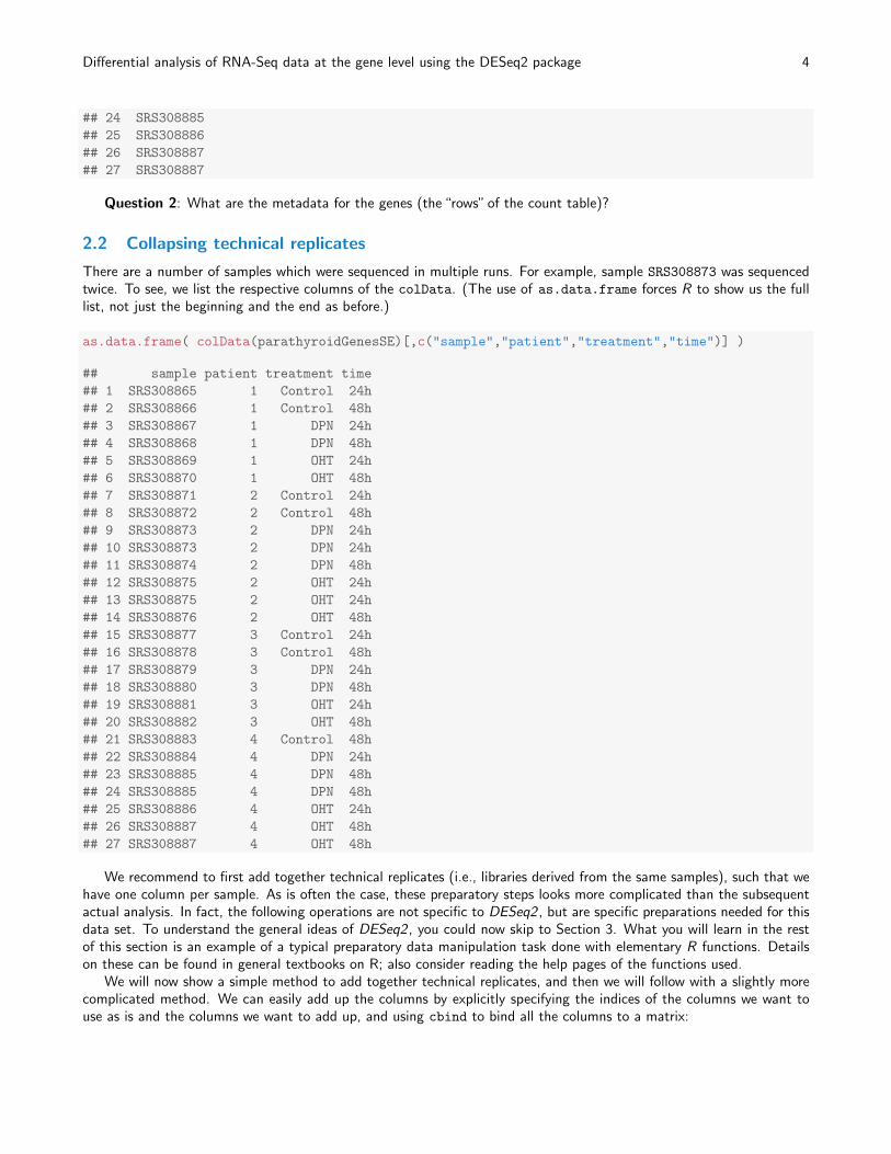
Question 2: What are the metadata for the genes (the “rows” of the count table)?

2.2 Collapsing technical replicates

There are a number of samples which were sequenced in multiple runs. For example, sample SRS308873 was sequencedtwice. To see, we list the respective columns of the colData. (The use of as.data.frame forces R to show us the fulllist, not just the beginning and the end as before.)

as.data.frame( colData(parathyroidGenesSE)[,c("sample","patient","treatment","time")] )

## sample patient treatment time

## 1 SRS308865 1 Control 24h

## 2 SRS308866 1 Control 48h

## 3 SRS308867 1 DPN 24h

## 4 SRS308868 1 DPN 48h

## 5 SRS308869 1 OHT 24h

## 6 SRS308870 1 OHT 48h

## 7 SRS308871 2 Control 24h

## 8 SRS308872 2 Control 48h

## 9 SRS308873 2 DPN 24h

## 10 SRS308873 2 DPN 24h

## 11 SRS308874 2 DPN 48h

## 12 SRS308875 2 OHT 24h

## 13 SRS308875 2 OHT 24h

## 14 SRS308876 2 OHT 48h

## 15 SRS308877 3 Control 24h

## 16 SRS308878 3 Control 48h

## 17 SRS308879 3 DPN 24h

## 18 SRS308880 3 DPN 48h

## 19 SRS308881 3 OHT 24h

## 20 SRS308882 3 OHT 48h

## 21 SRS308883 4 Control 48h

## 22 SRS308884 4 DPN 24h

## 23 SRS308885 4 DPN 48h

## 24 SRS308885 4 DPN 48h

## 25 SRS308886 4 OHT 24h

## 26 SRS308887 4 OHT 48h

## 27 SRS308887 4 OHT 48h

We recommend to first add together technical replicates (i.e., libraries derived from the same samples), such that wehave one column per sample. As is often the case, these preparatory steps looks more complicated than the subsequentactual analysis. In fact, the following operations are not specific to DESeq2 , but are specific preparations needed for thisdata set. To understand the general ideas of DESeq2 , you could now skip to Section 3. What you will learn in the restof this section is an example of a typical preparatory data manipulation task done with elementary R functions. Detailson these can be found in general textbooks on R; also consider reading the help pages of the functions used.

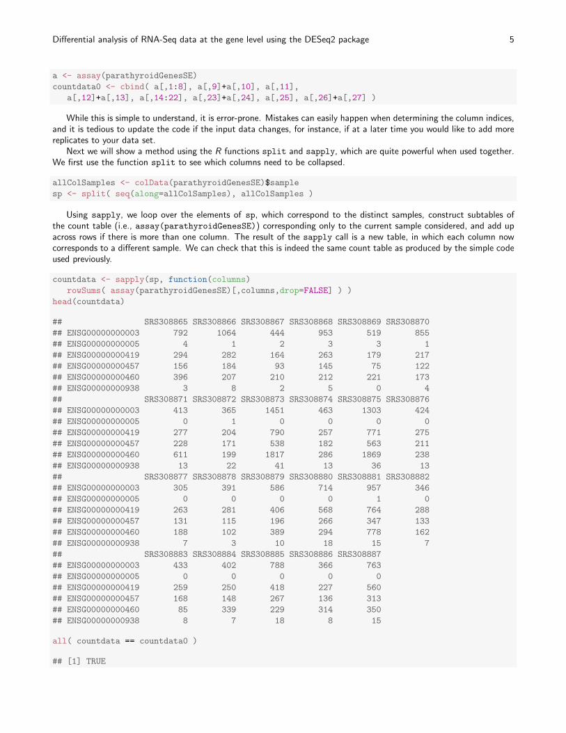
We will now show a simple method to add together technical replicates, and then we will follow with a slightly morecomplicated method. We can easily add up the columns by explicitly specifying the indices of the columns we want touse as is and the columns we want to add up, and using cbind to bind all the columns to a matrix:




a <- assay(parathyroidGenesSE)

countdata0 <- cbind( a[,1:8], a[,9]+a[,10], a[,11],

a[,12]+a[,13], a[,14:22], a[,23]+a[,24], a[,25], a[,26]+a[,27] )

While this is simple to understand, it is error-prone. Mistakes can easily happen when determining the column indices,and it is tedious to update the code if the input data changes, for instance, if at a later time you would like to add morereplicates to your data set.

Next we will show a method using the R functions split and sapply, which are quite powerful when used together.We first use the function split to see which columns need to be collapsed.

allColSamples <- colData(parathyroidGenesSE)$sample

sp <- split( seq(along=allColSamples), allColSamples )

Using sapply, we loop over the elements of sp, which correspond to the distinct samples, construct subtables ofthe count table (i.e., assay(parathyroidGenesSE)) corresponding only to the current sample considered, and add upacross rows if there is more than one column. The result of the sapply call is a new table, in which each column nowcorresponds to a different sample. We can check that this is indeed the same count table as produced by the simple codeused previously.

countdata <- sapply(sp, function(columns)

rowSums( assay(parathyroidGenesSE)[,columns,drop=FALSE] ) )

head(countdata)

## SRS308865 SRS308866 SRS308867 SRS308868 SRS308869 SRS308870

## ENSG00000000003 792 1064 444 953 519 855

## ENSG00000000005 4 1 2 3 3 1

## ENSG00000000419 294 282 164 263 179 217

## ENSG00000000457 156 184 93 145 75 122

## ENSG00000000460 396 207 210 212 221 173

## ENSG00000000938 3 8 2 5 0 4


## ENSG00000000003 413 365 1451 463 1303 424

## ENSG00000000005 0 1 0 0 0 0

## ENSG00000000419 277 204 790 257 771 275

## ENSG00000000457 228 171 538 182 563 211

## ENSG00000000460 611 199 1817 286 1869 238

## ENSG00000000938 13 22 41 13 36 13


## ENSG00000000003 305 391 586 714 957 346

## ENSG00000000005 0 0 0 0 1 0

## ENSG00000000419 263 281 406 568 764 288

## ENSG00000000457 131 115 196 266 347 133

## ENSG00000000460 188 102 389 294 778 162

## ENSG00000000938 7 3 10 18 15 7

## SRS308883 SRS308884 SRS308885 SRS308886 SRS308887

## ENSG00000000003 433 402 788 366 763

## ENSG00000000005 0 0 0 0 0

## ENSG00000000419 259 250 418 227 560

## ENSG00000000457 168 148 267 136 313

## ENSG00000000460 85 339 229 314 350

## ENSG00000000938 8 7 18 8 15

all( countdata == countdata0 )

## [1] TRUE


Having reduced our count data table to only one column per sample, we next need to subset the column metadataaccordingly, as we now have less columns. We also now use the sample names as names for the column data rows:

coldata <- colData(parathyroidGenesSE)[sapply(sp, `[`, 1),]

rownames(coldata) <- coldata$sample

coldata


## run experiment patient treatment time submission

## <character> <factor> <factor> <factor> <factor> <factor>

## SRS308865 SRR479052 SRX140503 1 Control 24h SRA051611


## SRS308867 SRR479054 SRX140505 1 DPN 24h SRA051611


## SRS308869 SRR479056 SRX140507 1 OHT 24h SRA051611

## ... ... ... ... ... ... ...






## study sample

## <factor> <factor>

## SRS308865 SRP012167 SRS308865

## SRS308866 SRP012167 SRS308866

## SRS308867 SRP012167 SRS308867

## SRS308868 SRP012167 SRS308868

## SRS308869 SRP012167 SRS308869

## ... ... ...

## SRS308883 SRP012167 SRS308883

## SRS308884 SRP012167 SRS308884

## SRS308885 SRP012167 SRS308885

## SRS308886 SRP012167 SRS308886

## SRS308887 SRP012167 SRS308887

Question 3: What do the quotation marks in the expression ‘[‘ do? What happens if you omit them?To unclutter the output in the subsequent steps, we only keep the column data columns that we actually need for

our analysis.

coldata <- coldata[ , c( "patient", "treatment", "time" ) ]

head( coldata )


## patient treatment time

## <factor> <factor> <factor>

## SRS308865 1 Control 24h


## SRS308867 1 DPN 24h

## SRS308868 1 DPN 48h

## SRS308869 1 OHT 24h

## SRS308870 1 OHT 48h

Our SummarizedExperiment object also contains metadata on the rows, which we can simply keep unchanged:


rowdata <- rowData(parathyroidGenesSE)

rowdata

## GRangesList of length 63193:

## $ENSG00000000003

## GRanges with 17 ranges and 2 metadata columns:

## seqnames ranges strand | exon_id exon_name

## <Rle> <IRanges> <Rle> | <integer> <character>

## [1] X [99883667, 99884983] - | 664095 ENSE00001459322

## [2] X [99885756, 99885863] - | 664096 ENSE00000868868

## [3] X [99887482, 99887565] - | 664097 ENSE00000401072

## [4] X [99887538, 99887565] - | 664098 ENSE00001849132

## [5] X [99888402, 99888536] - | 664099 ENSE00003554016

## ... ... ... ... ... ... ...

## [13] X [99890555, 99890743] - | 664106 ENSE00003512331

## [14] X [99891188, 99891686] - | 664108 ENSE00001886883

## [15] X [99891605, 99891803] - | 664109 ENSE00001855382

## [16] X [99891790, 99892101] - | 664110 ENSE00001863395

## [17] X [99894942, 99894988] - | 664111 ENSE00001828996

##

## ...

## <63192 more elements>

## ---

## seqlengths:

## 1 2 ... LRG_98 LRG_99

## 249250621 243199373 ... 18750 13294

We now have all the ingredients to prepare our data object in a form that is suitable for analysis, namely:� countdata: a table with the read counts, with technical replicates summed up,� coldata: a table with metadata on the count table’s columns, i.e., on the samples,� rowdata: a table with metadata on the count table’s rows, i.e., on the genes, and� a design formula, which tells which factors in the column metadata table specify the experimental design and how

these factors should be used in the analysis. We specify ∼ patient + treatment, which means that we want totest for the effect of treatment (the last factor), controlling for the effect of patient (the first factor). You can useR’s formula notation to express any experimental design that can be described within an ANOVA-like framework.

To now construct the data object from the matrix of counts and the metadata table, we use:

ddsFull <- DESeqDataSetFromMatrix(

countData = countdata,

colData = coldata,

design = ~ patient + treatment,

rowData = rowdata)

ddsFull

## class: DESeqDataSet

## dim: 63193 23

## exptData(0):

## assays(1): counts

## rownames(63193): ENSG00000000003 ENSG00000000005 ... LRG_98 LRG_99

## rowData metadata column names(0):

## colnames(23): SRS308865 SRS308866 ... SRS308886 SRS308887

## colData names(3): patient treatment time


3 Running the DESeq2 pipeline

Here we will analyze a subset of the samples, namely those taken after 48 hours, with either control or DPN treatment,taking into account the multifactor design.

3.1 Preparing the data object for the analysis of interest

First we subset the relevant columns from the full dataset:

dds <- ddsFull[ , colData(ddsFull)$treatment %in% c("Control","DPN") &

colData(ddsFull)$time == "48h" ]

Sometimes it is necessary to “refactor” the factors, in case that levels have been dropped. (Here, for example, thetreatment factor still contains the level “OHT”, but no sample to this level.)

dds$patient <- factor(dds$patient)

dds$treatment <- factor(dds$treatment)

It will be convenient to make sure that Control is the first level in the treatment factor, so that the log2 fold changesare calculated as treatment over control. The function relevel achieves this:

dds$treatment <- relevel( dds$treatment, "Control" )

We can also remove rows which have zero counts for all samples, as these will be ignored in subsequent analyis. It isnot necessary to perform this step, though it will make cleaner print-outs in the following sections.

dds <- dds[rowSums(counts(dds)) > 0,]

A quick check whether we now have the right samples:

colData(dds)


## patient treatment time

## <factor> <factor> <factor>


## SRS308868 1 DPN 48h


## SRS308874 2 DPN 48h


## SRS308880 3 DPN 48h


## SRS308885 4 DPN 48h

3.2 Running the pipeline

With the data object prepared, the DESeq2 analysis can now be run with a single call to the function DESeq:

dds <- DESeq(dds)

## estimating size factors

## estimating dispersions

## gene-wise dispersion estimates

## mean-dispersion relationship



## final dispersion estimates

## 1 rows did not converge in dispersion, labelled in mcols(object)£dispConv. Use larger maxit ar-

gument with estimateDispersions

## fitting model and testing

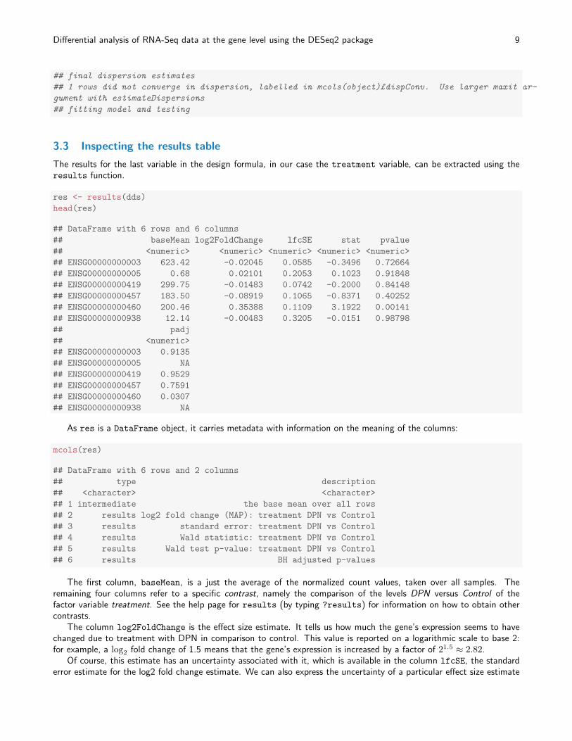
3.3 Inspecting the results table

The results for the last variable in the design formula, in our case the treatment variable, can be extracted using theresults function.

res <- results(dds)

head(res)


## baseMean log2FoldChange lfcSE stat pvalue

## <numeric> <numeric> <numeric> <numeric> <numeric>

## ENSG00000000003 623.42 -0.02045 0.0585 -0.3496 0.72664

## ENSG00000000005 0.68 0.02101 0.2053 0.1023 0.91848

## ENSG00000000419 299.75 -0.01483 0.0742 -0.2000 0.84148

## ENSG00000000457 183.50 -0.08919 0.1065 -0.8371 0.40252

## ENSG00000000460 200.46 0.35388 0.1109 3.1922 0.00141

## ENSG00000000938 12.14 -0.00483 0.3205 -0.0151 0.98798

## padj

## <numeric>

## ENSG00000000003 0.9135

## ENSG00000000005 NA

## ENSG00000000419 0.9529

## ENSG00000000457 0.7591

## ENSG00000000460 0.0307

## ENSG00000000938 NA

As res is a DataFrame object, it carries metadata with information on the meaning of the columns:

mcols(res)


## type description

## <character> <character>

## 1 intermediate the base mean over all rows

## 2 results log2 fold change (MAP): treatment DPN vs Control

## 3 results standard error: treatment DPN vs Control

## 4 results Wald statistic: treatment DPN vs Control

## 5 results Wald test p-value: treatment DPN vs Control

## 6 results BH adjusted p-values

The first column, baseMean, is a just the average of the normalized count values, taken over all samples. Theremaining four columns refer to a specific contrast, namely the comparison of the levels DPN versus Control of thefactor variable treatment. See the help page for results (by typing ?results) for information on how to obtain othercontrasts.

The column log2FoldChange is the effect size estimate. It tells us how much the gene’s expression seems to havechanged due to treatment with DPN in comparison to control. This value is reported on a logarithmic scale to base 2:for example, a log2 fold change of 1.5 means that the gene’s expression is increased by a factor of 21.5 ≈ 2.82.

Of course, this estimate has an uncertainty associated with it, which is available in the column lfcSE, the standarderror estimate for the log2 fold change estimate. We can also express the uncertainty of a particular effect size estimate


as the result of a statistical test. The purpose of a test for differential expression is to test whether the data providessufficient evidence to conclude that this value is really different from zero (and that the sign is correct). DESeq2 performsfor each gene a hypothesis test to see whether evidence is sufficient to decide against the null hypothesis that there is noeffect of the treatment on the gene and that the observed difference between treatment and control was merely causedby experimental variability (i. e., the type of variability that you can just as well expect between different samples in thesame treatment group). As usual in statistics, the result of this test is reported as a p value, and it is found in the columnpvalue. (Remember that a p value indicates the probability that a fold change as strong as the observed one, or evenstronger, would be seen under the situation described by the null hypothesis.)

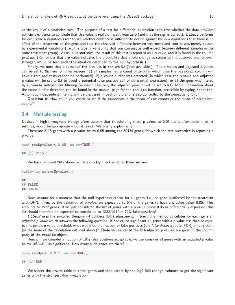
Finally, we note that a subset of the p values in res are NA (“not available”). The p values and adjusted p valuescan be set to NA here for three reasons: 1) all samples had a count of zero (in which case the baseMean column willhave a zero and tests cannot be performed); 2) a count outlier was detected (in which case the p value and adjustedp value will be set to NA to avoid a potential false positive call of differential expression); or 3) the gene was filteredby automatic independent filtering (in which case only the adjusted p-value will be set to NA). More information aboutthe count outlier detection can be found in the manual page for the results function, accessible by typing ?results.Automatic independent filtering will be discussed in Section 3.5 and is also controlled by the results function.

Question 4: How could you check to see if the baseMean is the mean of raw counts or the mean of normalizedcounts?

3.4 Multiple testing

Novices in high-throughput biology often assume that thresholding these p values at 0.05, as is often done in othersettings, would be appropriate – but it is not. We briefly explain why:

There are 2115 genes with a p value below 0.05 among the 30434 genes, for which the test succeeded in reporting ap value:

sum( res$pvalue < 0.05, na.rm=TRUE )

## [1] 2115

We have removed NAs above, so let’s quickly check whether there are any:

table( is.na(res$pvalue) )

##

## FALSE

## 30434

Now, assume for a moment that the null hypothesis is true for all genes, i.e., no gene is affected by the treatmentwith DPN. Then, by the definition of p value, we expect up to 5% of the genes to have a p value below 0.05. Thisamounts to 1522 genes. If we just considered the list of genes with a p value below 0.05 as differentially expressed, thislist should therefore be expected to contain up to 1522/2115 = 72% false positives!

DESeq2 uses the so-called Benjamini-Hochberg (BH) adjustment; in brief, this method calculates for each gene anadjusted p value which answers the following question: if one called significant all genes with a p value less than or equalto this gene’s p value threshold, what would be the fraction of false positives (the false discovery rate, FDR) among them(in the sense of the calculation outlined above)? These values, called the BH-adjusted p values, are given in the columnpadj of the results object.

Hence, if we consider a fraction of 10% false positives acceptable, we can consider all genes with an adjusted p valuebelow 10%=0.1 as significant. How many such genes are there?

sum( res$padj < 0.1, na.rm=TRUE )

## [1] 885

We subset the results table to these genes and then sort it by the log2-fold-change estimate to get the significantgenes with the strongest down-regulation



resSig <- res[ which(res$padj < 0.1 ), ]

head( resSig[ order( resSig$log2FoldChange ), ] )




## ENSG00000164089 101 -1.256 0.2270 -5.53 3.18e-08

## ENSG00000163631 269 -0.942 0.1033 -9.11 8.09e-20

## ENSG00000111181 114 -0.900 0.2640 -3.41 6.49e-04

## ENSG00000169239 1548 -0.753 0.1065 -7.07 1.50e-12

## ENSG00000041982 1493 -0.686 0.0922 -7.44 9.96e-14

## ENSG00000145244 173 -0.676 0.2556 -2.65 8.15e-03

## padj

## <numeric>

## ENSG00000164089 4.98e-06

## ENSG00000163631 7.18e-17

## ENSG00000111181 1.73e-02

## ENSG00000169239 6.65e-10

## ENSG00000041982 5.59e-11

## ENSG00000145244 9.92e-02

and with the strongest upregulation

tail( resSig[ order( resSig$log2FoldChange ), ] )




## ENSG00000005189 227 0.641 0.229 2.80 5.18e-03

## ENSG00000156414 137 0.727 0.138 5.27 1.40e-07

## ENSG00000103257 168 0.780 0.151 5.16 2.51e-07

## ENSG00000101255 285 0.797 0.186 4.29 1.76e-05

## ENSG00000130720 113 0.846 0.216 3.92 8.78e-05

## ENSG00000092621 594 0.869 0.151 5.76 8.33e-09

## padj

## <numeric>

## ENSG00000005189 7.42e-02

## ENSG00000156414 1.70e-05

## ENSG00000103257 2.68e-05

## ENSG00000101255 1.10e-03

## ENSG00000130720 3.74e-03

## ENSG00000092621 1.48e-06

Question 5: What is the proportion of down- and up-regulation among the genes with adjusted p value less than0.1?

3.5 Independent filtering

For weakly expressed genes, there is little chance of seeing differential expression, because the low read counts suffer fromsuch high Poisson noise that any biological effect is drowned in the uncertainties from the read counting. For example,imagine the control group has around an average count of 2, and the treatment group has around an average countof 1; without sequencing many biological replicates, this log2 fold change of -1 will be obscured by the randomness ofsampling at such low rates. By removing the weakly-expressed genes from the input to the FDR procedure, we can findmore genes to be significant among those which are kept, and so improve the power of our test.


For this reason, DESeq2 automatically performs independent filtering on the mean of the normalized counts, in orderto optimize the number of genes with FDR less than a threshold, which is set by default to 0.1. The mean of normalizedcounts is called a “filter statistic” in this case. The term independent highlights an important caveat. Such filtering ispermissible only if the filter statistic is independent of the actual test statistic [1]. Otherwise, the filtering would invalidatethe test and consequently the assumptions of the BH procedure. This is why we filter on the average over all samples:this filter is blind to the assignment of samples to the treatment and control group and hence independent.

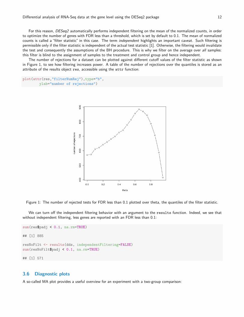
The number of rejections for a dataset can be plotted against different cutoff values of the filter statistic as shownin Figure 1, to see how filtering increases power. A table of the number of rejections over the quantiles is stored as anattribute of the results object res, accessible using the attr function:

plot(attr(res,"filterNumRej"),type="b",

ylab="number of rejections")

Figure 1: The number of rejected tests for FDR less than 0.1 plotted over theta, the quantiles of the filter statistic.

We can turn off the independent filtering behavior with an argument to the results function. Indeed, we see thatwithout independent filtering, less genes are reported with an FDR less than 0.1:

sum(res$padj < 0.1, na.rm=TRUE)

## [1] 885

resNoFilt <- results(dds, independentFiltering=FALSE)

sum(resNoFilt$padj < 0.1, na.rm=TRUE)

## [1] 571

3.6 Diagnostic plots

A so-called MA plot provides a useful overview for an experiment with a two-group comparison:



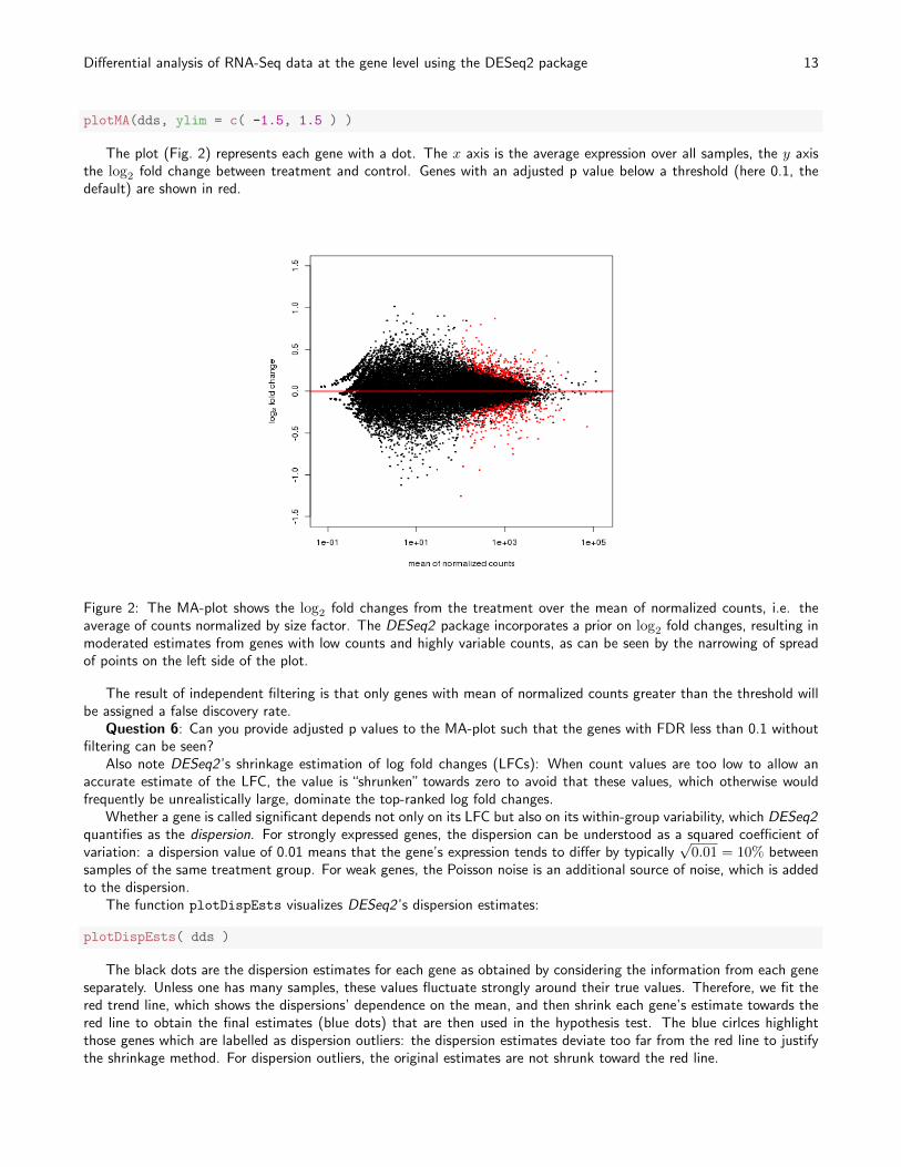
plotMA(dds, ylim = c( -1.5, 1.5 ) )

The plot (Fig. 2) represents each gene with a dot. The x axis is the average expression over all samples, the y axisthe log2 fold change between treatment and control. Genes with an adjusted p value below a threshold (here 0.1, thedefault) are shown in red.

Figure 2: The MA-plot shows the log2 fold changes from the treatment over the mean of normalized counts, i.e. theaverage of counts normalized by size factor. The DESeq2 package incorporates a prior on log2 fold changes, resulting inmoderated estimates from genes with low counts and highly variable counts, as can be seen by the narrowing of spreadof points on the left side of the plot.

The result of independent filtering is that only genes with mean of normalized counts greater than the threshold willbe assigned a false discovery rate.

Question 6: Can you provide adjusted p values to the MA-plot such that the genes with FDR less than 0.1 withoutfiltering can be seen?

Also note DESeq2 ’s shrinkage estimation of log fold changes (LFCs): When count values are too low to allow anaccurate estimate of the LFC, the value is “shrunken” towards zero to avoid that these values, which otherwise wouldfrequently be unrealistically large, dominate the top-ranked log fold changes.

Whether a gene is called significant depends not only on its LFC but also on its within-group variability, which DESeq2quantifies as the dispersion. For strongly expressed genes, the dispersion can be understood as a squared coefficient ofvariation: a dispersion value of 0.01 means that the gene’s expression tends to differ by typically

√0.01 = 10% between

samples of the same treatment group. For weak genes, the Poisson noise is an additional source of noise, which is addedto the dispersion.

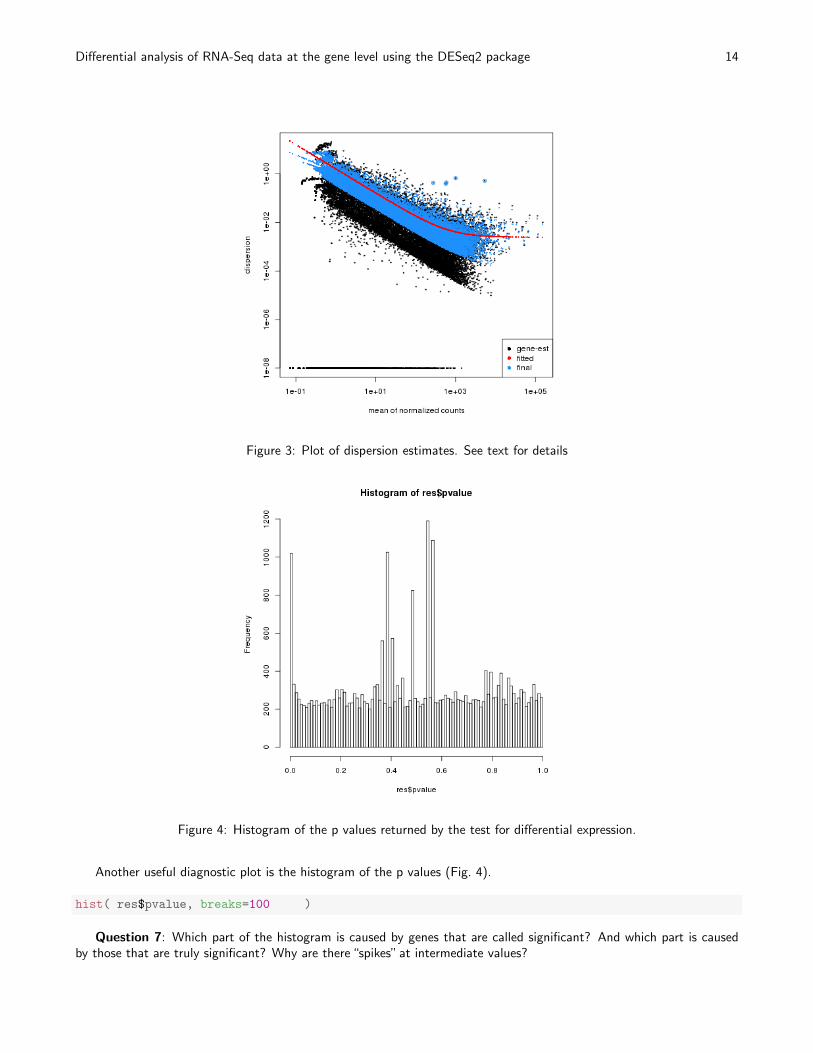
The function plotDispEsts visualizes DESeq2 ’s dispersion estimates:

plotDispEsts( dds )

The black dots are the dispersion estimates for each gene as obtained by considering the information from each geneseparately. Unless one has many samples, these values fluctuate strongly around their true values. Therefore, we fit thered trend line, which shows the dispersions’ dependence on the mean, and then shrink each gene’s estimate towards thered line to obtain the final estimates (blue dots) that are then used in the hypothesis test. The blue cirlces highlightthose genes which are labelled as dispersion outliers: the dispersion estimates deviate too far from the red line to justifythe shrinkage method. For dispersion outliers, the original estimates are not shrunk toward the red line.






Figure 3: Plot of dispersion estimates. See text for details

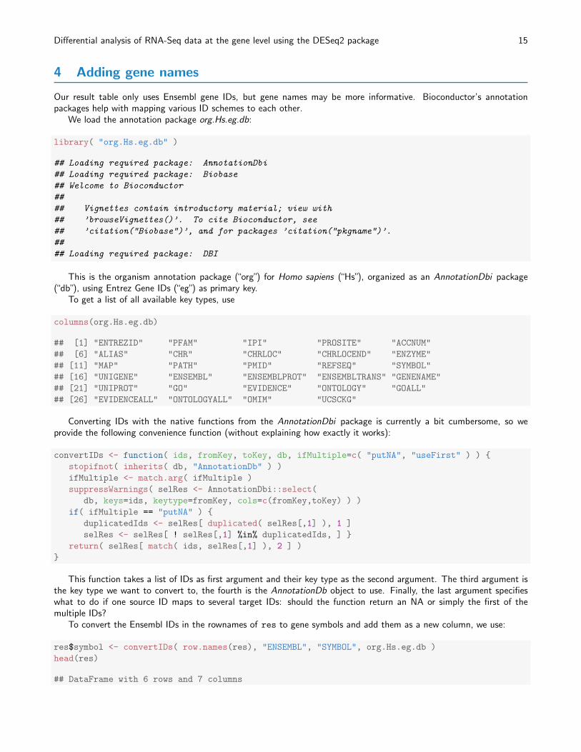
Figure 4: Histogram of the p values returned by the test for differential expression.

Another useful diagnostic plot is the histogram of the p values (Fig. 4).

hist( res$pvalue, breaks=100 )

Question 7: Which part of the histogram is caused by genes that are called significant? And which part is causedby those that are truly significant? Why are there “spikes” at intermediate values?


4 Adding gene names

Our result table only uses Ensembl gene IDs, but gene names may be more informative. Bioconductor’s annotationpackages help with mapping various ID schemes to each other.

We load the annotation package org.Hs.eg.db:

library( "org.Hs.eg.db" )

## Loading required package: AnnotationDbi

## Loading required package: Biobase

## Welcome to Bioconductor

##

## Vignettes contain introductory material; view with

## ’browseVignettes()’. To cite Bioconductor, see

## ’citation("Biobase")’, and for packages ’citation("pkgname")’.

##

## Loading required package: DBI

This is the organism annotation package (“org”) for Homo sapiens (“Hs”), organized as an AnnotationDbi package(“db”), using Entrez Gene IDs (“eg”) as primary key.

To get a list of all available key types, use

columns(org.Hs.eg.db)

## [1] "ENTREZID" "PFAM" "IPI" "PROSITE" "ACCNUM"

## [6] "ALIAS" "CHR" "CHRLOC" "CHRLOCEND" "ENZYME"

## [11] "MAP" "PATH" "PMID" "REFSEQ" "SYMBOL"

## [16] "UNIGENE" "ENSEMBL" "ENSEMBLPROT" "ENSEMBLTRANS" "GENENAME"

## [21] "UNIPROT" "GO" "EVIDENCE" "ONTOLOGY" "GOALL"

## [26] "EVIDENCEALL" "ONTOLOGYALL" "OMIM" "UCSCKG"

Converting IDs with the native functions from the AnnotationDbi package is currently a bit cumbersome, so weprovide the following convenience function (without explaining how exactly it works):

convertIDs <- function( ids, fromKey, toKey, db, ifMultiple=c( "putNA", "useFirst" ) ) {

stopifnot( inherits( db, "AnnotationDb" ) )

ifMultiple <- match.arg( ifMultiple )

suppressWarnings( selRes <- AnnotationDbi::select(

db, keys=ids, keytype=fromKey, cols=c(fromKey,toKey) ) )

if( ifMultiple == "putNA" ) {

duplicatedIds <- selRes[ duplicated( selRes[,1] ), 1 ]

selRes <- selRes[ ! selRes[,1] %in% duplicatedIds, ] }

return( selRes[ match( ids, selRes[,1] ), 2 ] )

}

This function takes a list of IDs as first argument and their key type as the second argument. The third argument isthe key type we want to convert to, the fourth is the AnnotationDb object to use. Finally, the last argument specifieswhat to do if one source ID maps to several target IDs: should the function return an NA or simply the first of themultiple IDs?

To convert the Ensembl IDs in the rownames of res to gene symbols and add them as a new column, we use:

res$symbol <- convertIDs( row.names(res), "ENSEMBL", "SYMBOL", org.Hs.eg.db )

head(res)


http://bioconductor.org/packages/release/data/annotation/html/org.Hs.eg.db.html

http://bioconductor.org/packages/release/bioc/html/AnnotationDbi.html





## ENSG00000000003 623.42 -0.02045 0.0585 -0.3496 0.72664

## ENSG00000000005 0.68 0.02101 0.2053 0.1023 0.91848

## ENSG00000000419 299.75 -0.01483 0.0742 -0.2000 0.84148

## ENSG00000000457 183.50 -0.08919 0.1065 -0.8371 0.40252

## ENSG00000000460 200.46 0.35388 0.1109 3.1922 0.00141

## ENSG00000000938 12.14 -0.00483 0.3205 -0.0151 0.98798

## padj symbol

## <numeric> <character>

## ENSG00000000003 0.9135 TSPAN6

## ENSG00000000005 NA TNMD

## ENSG00000000419 0.9529 DPM1

## ENSG00000000457 0.7591 SCYL3

## ENSG00000000460 0.0307 C1orf112

## ENSG00000000938 NA FGR

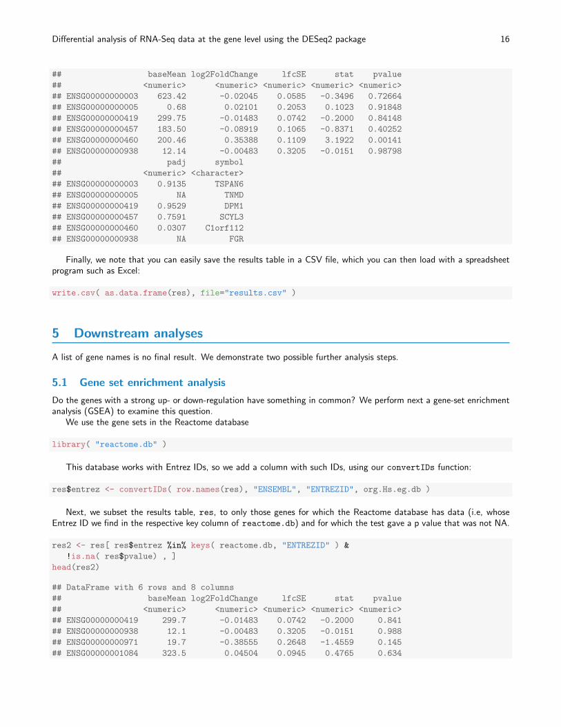
Finally, we note that you can easily save the results table in a CSV file, which you can then load with a spreadsheetprogram such as Excel:

write.csv( as.data.frame(res), file="results.csv" )

5 Downstream analyses

A list of gene names is no final result. We demonstrate two possible further analysis steps.

5.1 Gene set enrichment analysis

Do the genes with a strong up- or down-regulation have something in common? We perform next a gene-set enrichmentanalysis (GSEA) to examine this question.

We use the gene sets in the Reactome database

library( "reactome.db" )

This database works with Entrez IDs, so we add a column with such IDs, using our convertIDs function:

res$entrez <- convertIDs( row.names(res), "ENSEMBL", "ENTREZID", org.Hs.eg.db )

Next, we subset the results table, res, to only those genes for which the Reactome database has data (i.e, whoseEntrez ID we find in the respective key column of reactome.db) and for which the test gave a p value that was not NA.

res2 <- res[ res$entrez %in% keys( reactome.db, "ENTREZID" ) &

!is.na( res$pvalue) , ]

head(res2)




## ENSG00000000419 299.7 -0.01483 0.0742 -0.2000 0.841

## ENSG00000000938 12.1 -0.00483 0.3205 -0.0151 0.988

## ENSG00000000971 19.7 -0.38555 0.2648 -1.4559 0.145

## ENSG00000001084 323.5 0.04504 0.0945 0.4765 0.634


## ENSG00000001167 412.4 -0.05387 0.1031 -0.5225 0.601

## ENSG00000001626 11.0 0.15267 0.2988 0.5109 0.609

## padj symbol entrez

## <numeric> <character> <character>

## ENSG00000000419 0.953 DPM1 8813

## ENSG00000000938 NA FGR 2268

## ENSG00000000971 NA CFH 3075

## ENSG00000001084 0.880 GCLC 2729

## ENSG00000001167 0.870 NFYA 4800

## ENSG00000001626 NA CFTR 1080

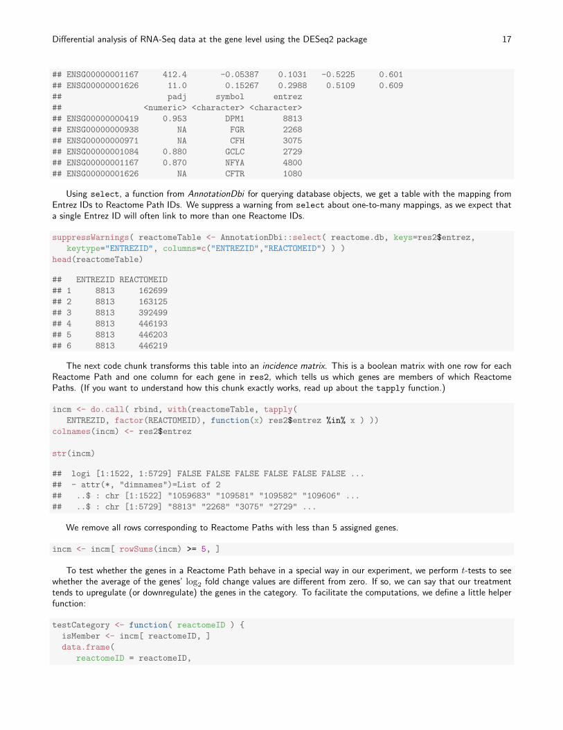
Using select, a function from AnnotationDbi for querying database objects, we get a table with the mapping fromEntrez IDs to Reactome Path IDs. We suppress a warning from select about one-to-many mappings, as we expect thata single Entrez ID will often link to more than one Reactome IDs.

suppressWarnings( reactomeTable <- AnnotationDbi::select( reactome.db, keys=res2$entrez,

keytype="ENTREZID", columns=c("ENTREZID","REACTOMEID") ) )

head(reactomeTable)

## ENTREZID REACTOMEID

## 1 8813 162699

## 2 8813 163125

## 3 8813 392499

## 4 8813 446193

## 5 8813 446203

## 6 8813 446219

The next code chunk transforms this table into an incidence matrix. This is a boolean matrix with one row for eachReactome Path and one column for each gene in res2, which tells us which genes are members of which ReactomePaths. (If you want to understand how this chunk exactly works, read up about the tapply function.)

incm <- do.call( rbind, with(reactomeTable, tapply(

ENTREZID, factor(REACTOMEID), function(x) res2$entrez %in% x ) ))

colnames(incm) <- res2$entrez

str(incm)

## logi [1:1522, 1:5729] FALSE FALSE FALSE FALSE FALSE FALSE ...

## - attr(*, "dimnames")=List of 2

## ..$ : chr [1:1522] "1059683" "109581" "109582" "109606" ...

## ..$ : chr [1:5729] "8813" "2268" "3075" "2729" ...

We remove all rows corresponding to Reactome Paths with less than 5 assigned genes.

incm <- incm[ rowSums(incm) >= 5, ]

To test whether the genes in a Reactome Path behave in a special way in our experiment, we perform t-tests to seewhether the average of the genes’ log2 fold change values are different from zero. If so, we can say that our treatmenttends to upregulate (or downregulate) the genes in the category. To facilitate the computations, we define a little helperfunction:

testCategory <- function( reactomeID ) {

isMember <- incm[ reactomeID, ]

data.frame(

reactomeID = reactomeID,



numGenes = sum( isMember ),

avgLFC = mean( res2$log2FoldChange[isMember] ),

strength = sum( res2$log2FoldChange[isMember] ) / sqrt(sum(isMember)),

pvalue = t.test( res2$log2FoldChange[ isMember ] )$p.value,

reactomeName = reactomePATHID2NAME[[reactomeID]] ) }

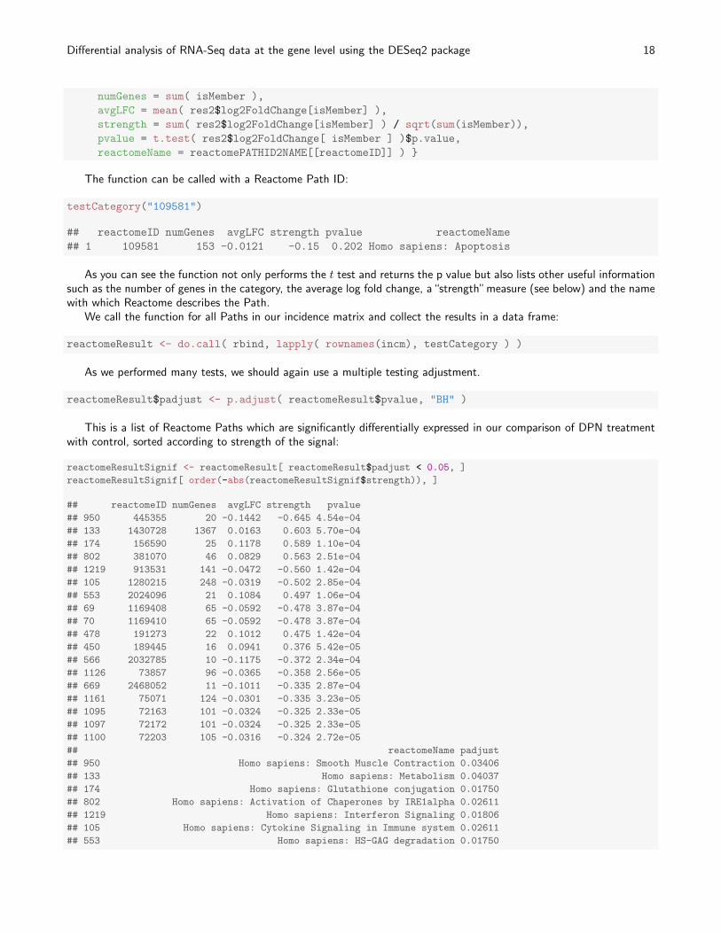
The function can be called with a Reactome Path ID:

testCategory("109581")

## reactomeID numGenes avgLFC strength pvalue reactomeName

## 1 109581 153 -0.0121 -0.15 0.202 Homo sapiens: Apoptosis

As you can see the function not only performs the t test and returns the p value but also lists other useful informationsuch as the number of genes in the category, the average log fold change, a“strength”measure (see below) and the namewith which Reactome describes the Path.

We call the function for all Paths in our incidence matrix and collect the results in a data frame:

reactomeResult <- do.call( rbind, lapply( rownames(incm), testCategory ) )

As we performed many tests, we should again use a multiple testing adjustment.

reactomeResult$padjust <- p.adjust( reactomeResult$pvalue, "BH" )

This is a list of Reactome Paths which are significantly differentially expressed in our comparison of DPN treatmentwith control, sorted according to strength of the signal:

reactomeResultSignif <- reactomeResult[ reactomeResult$padjust < 0.05, ]

reactomeResultSignif[ order(-abs(reactomeResultSignif$strength)), ]

## reactomeID numGenes avgLFC strength pvalue

## 950 445355 20 -0.1442 -0.645 4.54e-04

## 133 1430728 1367 0.0163 0.603 5.70e-04

## 174 156590 25 0.1178 0.589 1.10e-04

## 802 381070 46 0.0829 0.563 2.51e-04

## 1219 913531 141 -0.0472 -0.560 1.42e-04

## 105 1280215 248 -0.0319 -0.502 2.85e-04

## 553 2024096 21 0.1084 0.497 1.06e-04

## 69 1169408 65 -0.0592 -0.478 3.87e-04

## 70 1169410 65 -0.0592 -0.478 3.87e-04

## 478 191273 22 0.1012 0.475 1.42e-04

## 450 189445 16 0.0941 0.376 5.42e-05

## 566 2032785 10 -0.1175 -0.372 2.34e-04

## 1126 73857 96 -0.0365 -0.358 2.56e-05

## 669 2468052 11 -0.1011 -0.335 2.87e-04

## 1161 75071 124 -0.0301 -0.335 3.23e-05

## 1095 72163 101 -0.0324 -0.325 2.33e-05

## 1097 72172 101 -0.0324 -0.325 2.33e-05

## 1100 72203 105 -0.0316 -0.324 2.72e-05

## reactomeName padjust

## 950 Homo sapiens: Smooth Muscle Contraction 0.03406

## 133 Homo sapiens: Metabolism 0.04037

## 174 Homo sapiens: Glutathione conjugation 0.01750

## 802 Homo sapiens: Activation of Chaperones by IRE1alpha 0.02611

## 1219 Homo sapiens: Interferon Signaling 0.01806

## 105 Homo sapiens: Cytokine Signaling in Immune system 0.02611

## 553 Homo sapiens: HS-GAG degradation 0.01750


## 69 Homo sapiens: ISG15 antiviral mechanism 0.03084

## 70 Homo sapiens: Antiviral mechanism by IFN-stimulated genes 0.03084

## 478 Homo sapiens: Cholesterol biosynthesis 0.01806

## 450 Homo sapiens: Metabolism of porphyrins 0.01152

## 566 Homo sapiens: YAP1- and WWTR1 (TAZ)-stimulated gene expression 0.02611

## 1126 Homo sapiens: RNA Polymerase II Transcription 0.00822

## 669 Homo sapiens: Establishment of Sister Chromatid Cohesion 0.02611

## 1161 Homo sapiens: mRNA Processing 0.00822

## 1095 Homo sapiens: mRNA Splicing - Major Pathway 0.00822

## 1097 Homo sapiens: mRNA Splicing 0.00822

## 1100 Homo sapiens: Processing of Capped Intron-Containing Pre-mRNA 0.00822

Note that such lists need to be interpreted with care, and a grain of salt. Which of these categories make sense, giventhe biology of the experiment?

5.2 Nearest peak to a differentially expressed gene

The RNA-Seq experiment analyzed above provides a list of genes which have responded to a selective estrogen-receptor-beta agonist. We can investigate whether we find estrogen receptor binding sites in the vicinity of the gene with thehighest fold induction. In order to match differentially expressed genes to other experiment data, we will use annotatedbinding sites of estrogen receptor alpha from the ENCODE project. It is not necessarily the case that these annotatedbinding sites are actually functional in the cell lines of the RNA-Seq experiment or biologically relevant as the alphaand beta subtypes are distinct proteins transcribed from different genes; here we only use these binding site data fordemonstration purposes.

Let us consider a particular gene with a low p value. The rowData function provides us with all the informationabout the gene model; each of the exons is represented as a GRanges, and these are tied together as a GRangesList. Weuse the function range to extract the entire range of the gene, from the start of the left-most exon to the end of theright-most exon. This is all the information we need in order to find the nearest binding site.

deGeneID <- "ENSG00000099194"

res[deGeneID,]

## DataFrame with 1 row and 8 columns



## ENSG00000099194 8794 0.421 0.0193 21.9 4.94e-106

## padj symbol entrez

## <numeric> <character> <character>

## ENSG00000099194 5.27e-102 SCD 6319

deGene <- range(rowData(dds[deGeneID,])[[1]])

names(deGene) <- deGeneID

deGene

## GRanges with 1 range and 0 metadata columns:

## seqnames ranges strand

## <Rle> <IRanges> <Rle>

## ENSG00000099194 10 [102106881, 102124591] +

## ---

## seqlengths:

## 1 2 ... LRG_98 LRG_99

## 249250621 243199373 ... 18750 13294

We would like to compare the location of this gene with the location of annotated estrogen receptor binding sites,provided by the UCSC Genome Browser. We must first alter the sequence name (the chromosome name) of the differ-entially expressed gene, as the Ensembl gene annotation does not use the“chr”prefix, which the UCSC chromosomes are


annotated with. (Note that we ignore here another complication, which is that the Ensembl sequence “MT” correspondsto the UCSC’s sequence“chrM”.) We use the paste0 function, which concatenates the character vectors provided withoutusing any separating characters. We then create a range which is 10 Mb to the left and right of the start of the deGene

object.

as.character(seqnames(deGene))

## [1] "10"

ucscChrom <- paste0("chr",as.character(seqnames(deGene)))

ucscRanges <- ranges(flank(deGene,width=10e6,both=TRUE))

subsetRange <- GRanges(ucscChrom, ucscRanges)

subsetRange




## ENSG00000099194 chr10 [92106881, 112106880] *

## ---

## seqlengths:

## chr10

## NA

We now provide code which would download a track from the UCSC Genome Browser, in our case a track containingtranscription factor binding sites obtained from ChIP-Seq experiments across various cell lines, generated by the ENCODEproject.

The track names and table names must match a track name provided by the UCSC Genome Browser. For moreinformation on these steps, see the detailed instructions in the vignette of the rtracklayer package.

##

## Please do not run this code if you do not have an internet connection,

## alternatively use the local file import in the next code chunk.

##

# library( "rtracklayer" )

# trackName <- "wgEncodeRegTfbsClusteredV2"

# tableName <- "wgEncodeRegTfbsClusteredV2"

# trFactor <- "ERalpha_a"

# mySession <- browserSession()

# ucscTable <- getTable(ucscTableQuery(mySession, track=trackName,

# range=subsetRange, table=tableName,

# name=trFactor))

Here we use a locally cached copy of ucscTable:

ucscTableFile <- "/share/home/teacher/EMBO_HTS/DESeq_lab/localUcscTable.csv"

ucscTable <- read.csv(ucscTableFile, stringsAsFactors=FALSE)

We now can use the downloaded table of annotated estrogen receptor peaks. Whether to use a cutoff on the providedpeak scores at this step, or what scores cutoff to use, depends on your experience with the specific transcription factorand the ChIP-Seq experiments used to define these peaks. It often makes sense to visualize tracks in a genome browserin order to get a sense of the qualitative difference between peaks of different scores.

We create a GRanges object, peaks, from the table obtained from UCSC, and then we convert the chromosomenames back to the Ensembl style using the global substitute function, gsub. Finally, we enforce that the sequence levelsof the peaks match the sequence levels of the differential expressed gene, which is necessary for performing the nearestmatching in the following code chunk.

http://bioconductor.org/packages/release/bioc/html/rtracklayer.html


peaks <- with(ucscTable, GRanges(chrom, IRanges(chromStart, chromEnd),

score=score))

seqlevels(peaks) <- gsub("chr(.+)","\\1",seqlevels(peaks))

seqlevels(peaks) <- seqlevels(deGene)

Now we have two GRanges objects, defined over the same chromosomes, so we can use the distanceToNearest

function from the package GRanges. This provides a Hits object, which contains the matches between the “query” andthe “subject”, the first and second arguments to the function, as well as the distance from the query to the subject.As we only have a single query, there should only be one nearest range in the subject. See the documentation via?distanceToNearest and ?Hits for more information on the options for the this matching step.

d2nearest <- distanceToNearest(deGene, peaks)

Question 8: What is the distance from the differentially expressed gene to all the peaks?We can now examine the object d2nearest. This tells us that the nearest peak is 44 base pairs from the differential

expressed gene.

d2nearest

## Hits of length 1

## queryLength: 1

## subjectLength: 168

## queryHits subjectHits distance

## <integer> <integer> <integer>

## 1 1 118 44

The function subjectHits is used to extract the index of the closest hit in the peaks object.

deGene




## ENSG00000099194 10 [102106881, 102124591] +

## ---

## seqlengths:

## 1 2 ... LRG_98 LRG_99

## 249250621 243199373 ... 18750 13294

peaks[subjectHits(d2nearest)]

## GRanges with 1 range and 1 metadata column:

## seqnames ranges strand | score

## <Rle> <IRanges> <Rle> | <integer>

## [1] 10 [102124636, 102124912] * | 76

## ---

## seqlengths:

## 1 2 ... LRG_98 LRG_99

## NA NA ... NA NA

Is 44 base pairs unexpectedly close? Here we make a simple plot of the starting points of the peaks and gene alongthe chromosome, to get a sense of the distribution of peaks and how surprised we should be with the distance of thenearest. To identify the nearest peak, we construct a logical vector peakNearest, which can be used to change the yvalue and the color of the point corresponding to the nearest peak.

http://bioconductor.org/packages/release/bioc/html/GRanges.html


plotRange <- start(deGene) + 1e6 * c(-1,1)

peakNearest <- ( seq_along(peaks) == subjectHits(d2nearest) )

plot(x=start(peaks), y=ifelse(peakNearest,.3,.2),

ylim=c(0,1), xlim=plotRange, pch='p',

col=ifelse(peakNearest,"red","grey60"),

yaxt="n", ylab="",

xlab=paste("2 Mb on chromosome",as.character(seqnames(deGene))))

points(x=start(deGene),y=.8,pch='g')

Figure 5: A 2 Mb genomic range showing the location of the differentially expressed gene (labelled ’g’), and the peaks(labelled ’p’). As there are only 14 peaks spread over 2 Mb, it is surprising to find a peak 44 base pairs away from thedifferentially expressed gene.

Again, the biological relevance of the distances between peaks and genes is another matter, especially considering thedata are from different sources. An important consideration when investigating the distribution of distances between twosets of genomic features, is how the individual sets cluster along the genome.

Question 9: Are the peaks relatively uniformly distributed?

6 Working with rlog-transformed data

6.1 The rlog transform

Many common statistical methods for exploratory analysis of multidimensional data, especially methods for clusteringand ordination (e. g., principal-component analysis and the like), work best for (at least approximately) homoskedasticdata; this means that the variance of an observable (i.e., here, the expression strength of a gene) does not depend on themean. In RNA-Seq data, however, variance grows with the mean. For example, if one performs PCA directly on a matrixof normalized read counts, the result typically depends only on the few most strongly expressed genes because they showthe largest absolute differences between samples. A simple and often used strategy to avoid this is to take the logarithmof the normalized count values; however, now the genes with low counts tend to dominate the results because, due tothe strong Poisson noise inherent to small count values, they show the strongest relative differences between samples.

As a solution, DESeq2 offers the regularized-logarithm transformation, or rlog for short. For genes with high counts,the rlog transformation differs not much from an ordinary log2 transformation. For genes with lower counts, however,the values are shrunken towards the genes’ averages across all samples. Using an empirical Bayesian prior in the form ofa ridge penality, this is done such that the rlog-transformed data are approximately homoskedastic.



The function rlogTransform returns a SummarizedExperiment object which contains the rlog-transformed values inits assay slot:

rld <- rlogTransformation(dds)

## you had estimated gene-wise dispersions, removing these

## you had estimated fitted dispersions, removing these

head( assay(rld) )


## ENSG00000000003 9.716 9.687 9.133 9.190 8.960 8.871

## ENSG00000000005 -0.679 -0.475 -0.629 -0.782 -0.783 -0.795

## ENSG00000000419 8.100 8.110 8.240 8.290 8.302 8.307

## ENSG00000000457 7.444 7.302 7.816 7.709 7.222 7.343

## ENSG00000000460 7.573 7.671 7.987 8.171 7.135 7.453

## ENSG00000000938 3.235 3.075 4.180 3.672 2.966 3.403

## SRS308883 SRS308885

## ENSG00000000003 9.094 9.114

## ENSG00000000005 -0.783 -0.793

## ENSG00000000419 8.264 8.172

## ENSG00000000457 7.601 7.495

## ENSG00000000460 7.017 7.375

## ENSG00000000938 3.368 3.500

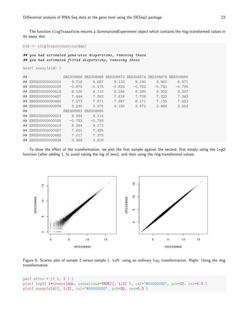
To show the effect of the transformation, we plot the first sample against the second, first simply using the log2

function (after adding 1, to avoid taking the log of zero), and then using the rlog-transformed values.

Figure 6: Scatter plot of sample 2 versus sample 1. Left: using an ordinary log2 transformation. Right: Using the rlogtransformation.

par( mfrow = c( 1, 2 ) )

plot( log2( 1+counts(dds, normalized=TRUE)[, 1:2] ), col="#00000020", pch=20, cex=0.3 )

plot( assay(rld)[, 1:2], col="#00000020", pch=20, cex=0.3 )


Note that, in order to make it easier to see where several points are plotted on top of each other, we set the plottingcolor to a semi-transparent black (encoded as #00000020) and changed the points to solid disks (pch=20) with reducedsize (cex=0.3)1.

In Figure 6, we can see how genes with low counts seem to be excessively variable on the ordinary logarithmic scale,while the rlog transform compresses differences for genes for which the data cannot provide good information anyway.

6.2 Sample distances

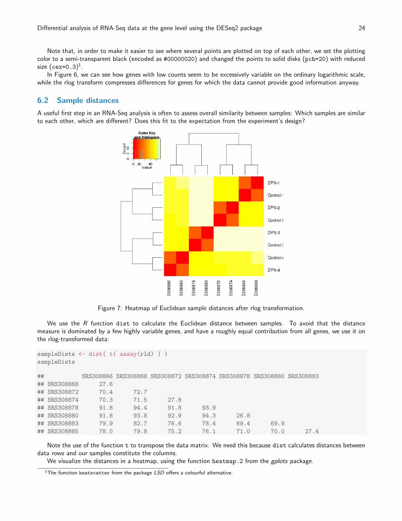
A useful first step in an RNA-Seq analysis is often to assess overall similarity between samples: Which samples are similarto each other, which are different? Does this fit to the expectation from the experiment’s design?

Figure 7: Heatmap of Euclidean sample distances after rlog transformation.

We use the R function dist to calculate the Euclidean distance between samples. To avoid that the distancemeasure is dominated by a few highly variable genes, and have a roughly equal contribution from all genes, we use it onthe rlog-transformed data:

sampleDists <- dist( t( assay(rld) ) )

sampleDists

## SRS308866 SRS308868 SRS308872 SRS308874 SRS308878 SRS308880 SRS308883

## SRS308868 27.6

## SRS308872 70.4 72.7

## SRS308874 70.3 71.5 27.8

## SRS308878 91.8 94.4 91.8 93.9

## SRS308880 91.8 93.8 92.9 94.3 26.8

## SRS308883 79.9 82.7 76.6 78.4 69.4 69.9

## SRS308885 78.0 79.8 75.2 76.1 71.0 70.0 27.4

Note the use of the function t to transpose the data matrix. We need this because dist calculates distances betweendata rows and our samples constitute the columns.

We visualize the distances in a heatmap, using the function heatmap.2 from the gplots package.

1The function heatscatter from the package LSD offers a colourful alternative.

http://cran.fhcrc.org/web/packages/gplots/index.html

http://cran.fhcrc.org/web/packages/LSD/index.html


sampleDistMatrix <- as.matrix( sampleDists )

rownames(sampleDistMatrix) <- paste( colData(rld)$treatment,

colData(rld)$patient, sep="-" )

library( "gplots" )

## KernSmooth 2.23 loaded

## Copyright M. P. Wand 1997-2009

##

## Attaching package: ’gplots’

##

## The following object is masked from ’package:IRanges’:

##

## space

##

## The following object is masked from ’package:stats’:

##

## lowess

heatmap.2( sampleDistMatrix, trace="none" )

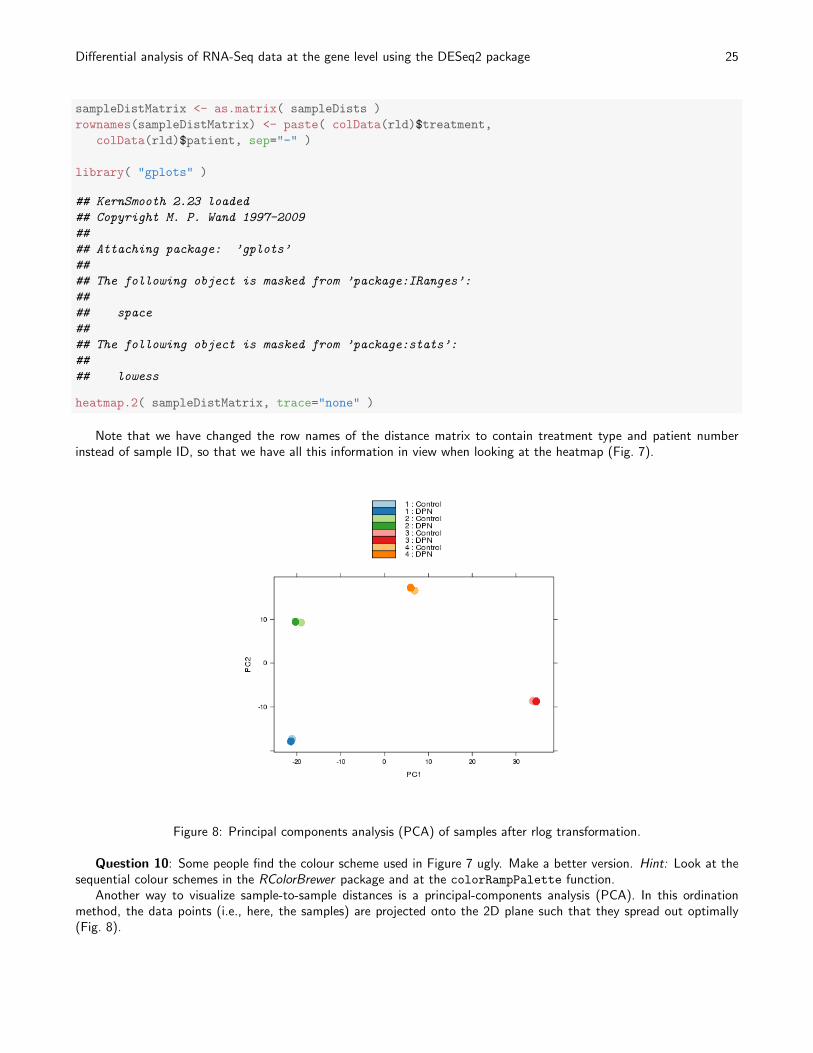
Note that we have changed the row names of the distance matrix to contain treatment type and patient numberinstead of sample ID, so that we have all this information in view when looking at the heatmap (Fig. 7).

Figure 8: Principal components analysis (PCA) of samples after rlog transformation.

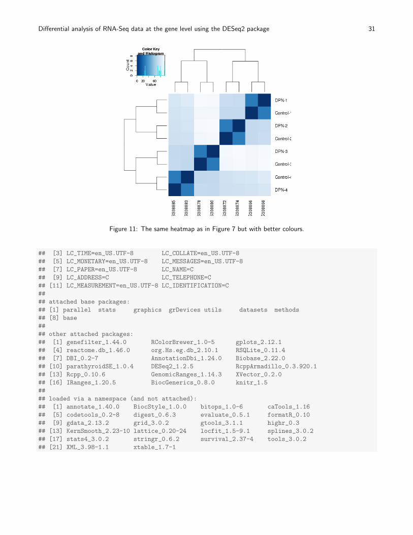
Question 10: Some people find the colour scheme used in Figure 7 ugly. Make a better version. Hint: Look at thesequential colour schemes in the RColorBrewer package and at the colorRampPalette function.

Another way to visualize sample-to-sample distances is a principal-components analysis (PCA). In this ordinationmethod, the data points (i.e., here, the samples) are projected onto the 2D plane such that they spread out optimally(Fig. 8).

http://cran.fhcrc.org/web/packages/RColorBrewer/index.html


print( plotPCA( rld, intgroup = c( "patient", "treatment") ) )

Here, we have used the function plotPCA which comes with DESeq2 . The two terms specified as intgroup arecolumn names from our sample data; they tell the function to use them to choose colours.

From both visualizations, we see that the differences between patients is much larger than the difference betweentreatment and control samples of the same patient. This shows why it was important to account for this paired design(“paired”, because each treated sample is paired with one control sample from the same patient). We did so by using thedesign formula !~ patient treatment! when setting up the data object in the beginning. Had we used an un-pairedanalysis, by specifying only ~ treatment, we would not have found many hits, because then, the patient-to-patientdifferences would have drowned out any treatment effects.

Here, we have performed this sample distance analysis towards the end of our analysis. In practice, however, this isa step suitable to give a first overview on the data. Hence, one will typically carry out this analysis as one of the firststeps in an analysis. To this end, you may also find the function arrayQualityMetrics, from the equinymous package,useful.

6.3 Gene clustering

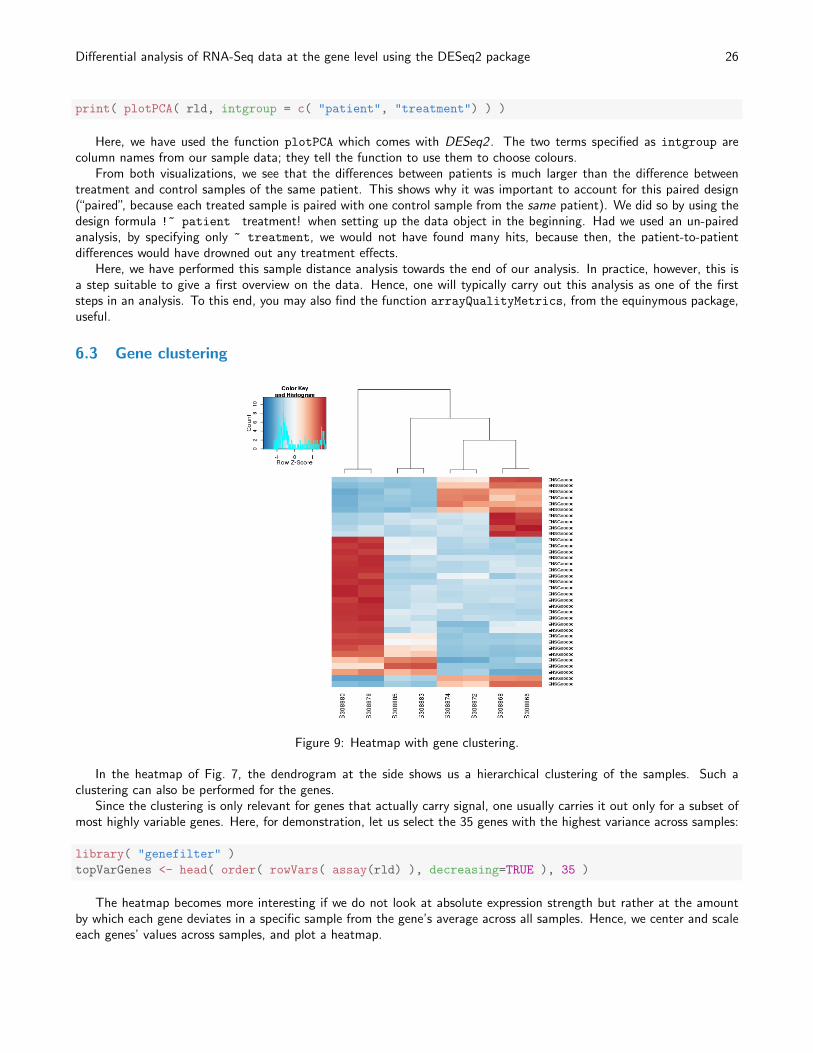
Figure 9: Heatmap with gene clustering.

In the heatmap of Fig. 7, the dendrogram at the side shows us a hierarchical clustering of the samples. Such aclustering can also be performed for the genes.

Since the clustering is only relevant for genes that actually carry signal, one usually carries it out only for a subset ofmost highly variable genes. Here, for demonstration, let us select the 35 genes with the highest variance across samples:

library( "genefilter" )

topVarGenes <- head( order( rowVars( assay(rld) ), decreasing=TRUE ), 35 )

The heatmap becomes more interesting if we do not look at absolute expression strength but rather at the amountby which each gene deviates in a specific sample from the gene’s average across all samples. Hence, we center and scaleeach genes’ values across samples, and plot a heatmap.



heatmap.2( assay(rld)[ topVarGenes, ], scale="row",

trace="none", dendrogram="column",

col = colorRampPalette( rev(brewer.pal(9, "RdBu")) )(255))

We can now see (Fig. 9) blocks of genes which covary across patients. Often, such a heatmap is insightful, eventhough here, seeing these variations across patients is of limited value because we are rather interested in the effectsbetween the two samples from each patient.

7 Advanced Questions

For these questions, we provide (and probably have) no solutions, advanced readers are encouraged to explore them.1. DESeq2 performs the shrinkage of the dispersion estimates by fitting a parametric curve on the mean of normalized

counts (cf. Figure 3). However, one could argue that the biological variability of genes should not be a function ofcounts, but of counts per gene length (i. e., expression level), and that regression on that covariate should lead toa better fit. Write your own version of the estimateDispersions function to explore this question.

2. What is the contribution of UTR length variations to the between-replicates variability modelled by DESeq2? Theread counting script (available in the vignette of parathyroidSE ) uses all exons of the genes, which includes UTRs.Would detection power be increased –or would we preferentially detect different phenomena– if we left out UTRsfrom the counting (i. e. count reads that fall on coding exons only); or indeed, if we looked only at UTRs?





8 Solutions

Answer 1:

nrow(parathyroidGenesSE)

## [1] 63193

Answer 2:

rowData( parathyroidGenesSE )

## GRangesList of length 63193:

## $ENSG00000000003

## GRanges with 17 ranges and 2 metadata columns:

## seqnames ranges strand | exon_id exon_name

## <Rle> <IRanges> <Rle> | <integer> <character>

## [1] X [99883667, 99884983] - | 664095 ENSE00001459322

## [2] X [99885756, 99885863] - | 664096 ENSE00000868868

## [3] X [99887482, 99887565] - | 664097 ENSE00000401072

## [4] X [99887538, 99887565] - | 664098 ENSE00001849132

## [5] X [99888402, 99888536] - | 664099 ENSE00003554016

## ... ... ... ... ... ... ...

## [13] X [99890555, 99890743] - | 664106 ENSE00003512331

## [14] X [99891188, 99891686] - | 664108 ENSE00001886883

## [15] X [99891605, 99891803] - | 664109 ENSE00001855382

## [16] X [99891790, 99892101] - | 664110 ENSE00001863395

## [17] X [99894942, 99894988] - | 664111 ENSE00001828996

##

## ...

## <63192 more elements>

## ---

## seqlengths:

## 1 2 ... LRG_98 LRG_99

## 249250621 243199373 ... 18750 13294

Answer 3:The function sapply expects an R function as its second argument. Here, we want to provide it with the function

for vector subsetting (as in a[1]), and the name of this function is [. However, if we provide that name without thequotation marks, the R interpreter gets confused and complains about the unexpected symbol (try this out). Hence weneed to quote the function name in our call to sapply.

Answer 4: The raw counts and normalized counts of a DESeqDataSet object are available via the accessor functioncounts, which has an argument normalized, which defaults to FALSE.

all.equal(res$baseMean, rowMeans(counts(dds)))

## [1] "names for current but not for target"

## [2] "Mean relative difference: 0.0582"

all.equal(res$baseMean, rowMeans(counts(dds,normalized=TRUE)))

## [1] "names for current but not for target"

Answer 5:


table(sign(resSig$log2FoldChange))

##

## -1 1

## 457 428

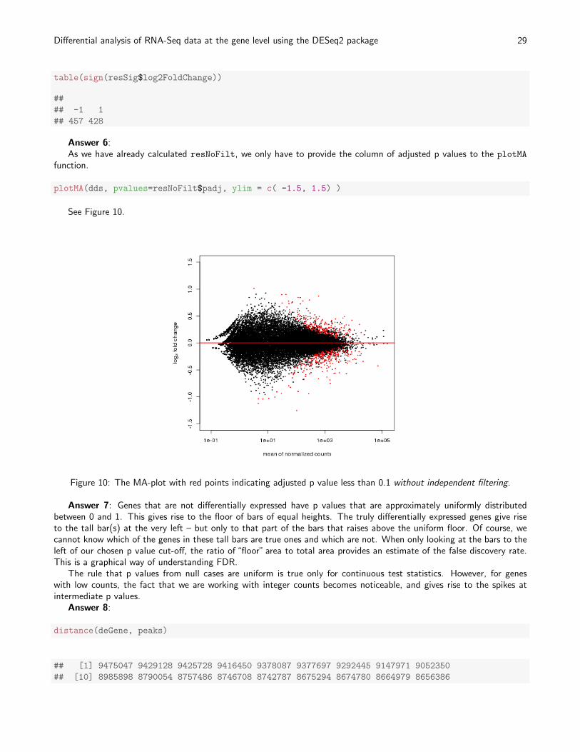
Answer 6:As we have already calculated resNoFilt, we only have to provide the column of adjusted p values to the plotMA

function.

plotMA(dds, pvalues=resNoFilt$padj, ylim = c( -1.5, 1.5) )

See Figure 10.

Figure 10: The MA-plot with red points indicating adjusted p value less than 0.1 without independent filtering.

Answer 7: Genes that are not differentially expressed have p values that are approximately uniformly distributedbetween 0 and 1. This gives rise to the floor of bars of equal heights. The truly differentially expressed genes give riseto the tall bar(s) at the very left – but only to that part of the bars that raises above the uniform floor. Of course, wecannot know which of the genes in these tall bars are true ones and which are not. When only looking at the bars to theleft of our chosen p value cut-off, the ratio of “floor” area to total area provides an estimate of the false discovery rate.This is a graphical way of understanding FDR.

The rule that p values from null cases are uniform is true only for continuous test statistics. However, for geneswith low counts, the fact that we are working with integer counts becomes noticeable, and gives rise to the spikes atintermediate p values.

Answer 8:

distance(deGene, peaks)

## [1] 9475047 9429128 9425728 9416450 9378087 9377697 9292445 9147971 9052350

## [10] 8985898 8790054 8757486 8746708 8742787 8675294 8674780 8664979 8656386


## [19] 8482847 8223783 8221925 8135509 8001210 7455663 7085829 6942799 6925411

## [28] 6901313 6888089 6884998 6881075 6880706 6864676 6780255 6775784 6605487

## [37] 6599859 6596686 6588697 6583718 6571499 6420064 6351948 6351146 6329893

## [46] 6319663 6310500 6310175 6308781 6304333 6293607 6288353 6271339 6268796

## [55] 6262968 5922099 5213835 5117195 5058165 5057764 5038070 4950763 4846639

## [64] 4840470 4690192 4604930 4150399 4075280 3867684 3837681 3750152 3728198

## [73] 3713689 3672012 3545140 3489164 3483060 3482656 3374532 3145464 3009849

## [82] 3009475 2945584 2938228 2898743 2780415 2775156 2772196 2766543 2697779

## [91] 2134525 2099928 2093216 2080614 2079696 2078669 2077381 2074629 2052830

## [100] 2050846 2044996 2044079 2043235 2032452 1972277 1970323 1864919 1843269

## [109] 1397487 951766 778762 566972 415890 336981 235041 45754 1220

## [118] 44 518646 536372 624809 727175 759664 988971 1236678 1267088

## [127] 1482084 1528951 1573655 1600301 1752606 1755604 1767986 1810760 1842340

## [136] 1962210 2003350 2039054 2048291 2137914 2293613 2342835 2345825 2347756

## [145] 2399792 2400158 2404602 2409590 2489595 2791121 2803606 2806523 2866416

## [154] 2867474 4107727 4108577 4109757 4112806 4115469 4116070 4198736 7246349

## [163] 9538145 9592618 9593558 9704719 9860874 9909237

Answer 9:We can answer this question by investigating the inter-peak distances. As all of our peaks are on the same chromosome,

we just sort the peak starts and subtract the 2nd from the 1st, the 3rd from the 2nd, etc. Then we call the summary

function which provides the mean and median. Note that the mean is constricted: it must be equal to the total spandivided by the number of inter-peak distances. The median distance is about one quarter of the mean, so the peaks tendto cluster. You can also verify this by plotting the histogram of peakDists.

peakDists <- diff(sort(start(peaks)))

summary(peakDists)

## Min. 1st Qu. Median Mean 3rd Qu. Max.

## 364 5110 32500 116000 103000 3050000

mean(peakDists)

## [1] 116181

Answer 10:

library("RColorBrewer")

colours = colorRampPalette( rev(brewer.pal(9, "Blues")) )(255)

heatmap.2( sampleDistMatrix, trace="none", col=colours)

See Figure 11.

9 Session Info

As last part of this document, we call the function sessionInfo, which reports the version numbers of R and all thepackages used in this session. It is good practice to always keep such a record as it will help to trace down what hashappened in case that an R script ceases to work because a package has been changed in a newer version.

## R version 3.0.2 (2013-09-25)

## Platform: x86_64-unknown-linux-gnu (64-bit)

##

## locale:

## [1] LC_CTYPE=en_US.UTF-8 LC_NUMERIC=C


Figure 11: The same heatmap as in Figure 7 but with better colours.

## [3] LC_TIME=en_US.UTF-8 LC_COLLATE=en_US.UTF-8

## [5] LC_MONETARY=en_US.UTF-8 LC_MESSAGES=en_US.UTF-8

## [7] LC_PAPER=en_US.UTF-8 LC_NAME=C

## [9] LC_ADDRESS=C LC_TELEPHONE=C

## [11] LC_MEASUREMENT=en_US.UTF-8 LC_IDENTIFICATION=C

##

## attached base packages:

## [1] parallel stats graphics grDevices utils datasets methods

## [8] base

##

## other attached packages:

## [1] genefilter_1.44.0 RColorBrewer_1.0-5 gplots_2.12.1

## [4] reactome.db_1.46.0 org.Hs.eg.db_2.10.1 RSQLite_0.11.4

## [7] DBI_0.2-7 AnnotationDbi_1.24.0 Biobase_2.22.0

## [10] parathyroidSE_1.0.4 DESeq2_1.2.5 RcppArmadillo_0.3.920.1

## [13] Rcpp_0.10.6 GenomicRanges_1.14.3 XVector_0.2.0

## [16] IRanges_1.20.5 BiocGenerics_0.8.0 knitr_1.5

##

## loaded via a namespace (and not attached):

## [1] annotate_1.40.0 BiocStyle_1.0.0 bitops_1.0-6 caTools_1.16

## [5] codetools_0.2-8 digest_0.6.3 evaluate_0.5.1 formatR_0.10

## [9] gdata_2.13.2 grid_3.0.2 gtools_3.1.1 highr_0.3

## [13] KernSmooth_2.23-10 lattice_0.20-24 locfit_1.5-9.1 splines_3.0.2

## [17] stats4_3.0.2 stringr_0.6.2 survival_2.37-4 tools_3.0.2

## [21] XML_3.98-1.1 xtable_1.7-1


References

[1] Richard Bourgon, Robert Gentleman, and Wolfgang Huber. Independent filtering increases detection power forhigh-throughput experiments. PNAS, 107(21):9546–9551, 2010.

differential analysis of rna-seq data at the gene level using the

Documents