differential constraints for the probability … · density function of stochastic solutions to the...

International Journal for Uncertainty Quantification, 2 (3): 195–213 (2012)

DIFFERENTIAL CONSTRAINTS FOR THEPROBABILITY DENSITY FUNCTION OF STOCHASTICSOLUTIONS TO THE WAVE EQUATION

Daniele Venturi & George Em Karniadakis∗

Division of Applied Mathematics, Brown University, Providence, Rhode Island 09212, USA

Original Manuscript Submitted: 05/16/2011; Final Draft Received: 07/26/2011

By using functional integral methods we determine new types of differential constraints satisfied by the joint probabilitydensity function of stochastic solutions to the wave equation subject to uncertain boundary and initial conditions. Thesedifferential constraints involve unusual limit partial differential operators and, in general, they can be grouped intotwo main classes: the first one depends on the specific field equation under consideration (i.e., on the stochastic waveequation), the second class includes a set of intrinsic relations determined by the structure of the joint probability densityfunction of the wave and its derivatives. Preliminary results we have obtained for stochastic dynamical systems andfirst-order nonlinear stochastic particle differential equations (PDEs) suggest that the set of differential constraints iscomplete and, therefore, it allows determining uniquely the probability density function of the solution to the stochasticproblem. The proposed new approach can be extended to arbitrary nonlinear stochastic PDEs and it could be an effectiveway to overcome the curse of dimensionality for random boundary and initial conditions. An application of the theorydeveloped is presented and discussed for a simple random wave in one spatial dimension.

KEY WORDS: stochastic partial differential equations, high-dimensional methods, random fields

1. INTRODUCTION

Many physical phenomena such as sound propagation, electromagnetic scattering at random surfaces, and randomvibrations in solid mechanics can be described in terms of random waves satisfying the standard wave equation

∂2ψ

∂t2= U2∇2ψ (1)

for random boundary conditions, random initial conditions, or random group velocity. The purpose of this paper isto introduce a new method to compute the statistical properties of the stochastic solutions to Eq. (1). This method isbased on a set of differential constraints for the joint probability density function of the waveψ and its derivativesand it may present an advantage with respect to more classical stochastic approaches such as polynomial chaos [1–4], probabilistic collocation [5, 6], and generalized spectral decompositions [7–11]. In fact, it seems that it does notsuffer from the curse of dimensionality problem, at least when randomness comes from boundary or initial conditions.Indeed, since we are solving for probability density function of the system, we can actually prescribe these conditionsin terms of the probability distributions and this is obviously not dependent on the number of random variablescharacterizing the underlying probability space.

This observation immediately leads us to the question: Is it possible to determine a closed evolution equation forthe probability density function of the solution to Eq. (1) at a specific space-time location? Unfortunately, the answeris negative. In fact, the self-interacting nature of the wave equation is associated with nonlocal solutions in space andtime that, in turn, yield the impossibility of determining a pointwise equation for the probability density function.

∗Correspond to George Em Karniadakis, E-mail: [email protected]

2152–5080/12/$35.00 c© 2012 by Begell House, Inc. 195

196 Venturi & Karniadakis

However, an equation for the probability density functional of the wave always can be obtained. This very generalapproach relies on the use of functional integral techniques [12–16]; in particular, those involving the Hopf character-istic functional (see Appendix B). These functional methods aim to cope with the global probabilistic structure of thesolution and they have been extensively studied in the past as a possible tool to tackle many fundamental problems inphysics such as turbulence [17, 18]. Their usage grew very rapidly in the 1970s, when it became clear that diagram-matic functional techniques [12] could be applied, at least formally, to many different problems in classical statisticalphysics. However, functional differential equations involving the Hopf characteristic functional unfortunately are notamenable to numerical simulation. In addition, the amount of statistical information carried on by the Hopf character-istic functional is often far beyond the needs of practical uncertainty quantification, which usually reduces only to thecomputation of a few statistical moments of the solution at specific space-time locations.

Thus, we are led to look for alternative ways to determine the evolution of the probability density function asso-ciated with the solution to Eq. (1). To this end, by using a functional integral technique we have introduced recentlyin the context of stochastic dynamical systems, in this paper we will show that it is possible to formulate a set of dif-ferential constraints that have to be satisfied locally by the probability density function of every random wave processgoverned by Eq. (1). These constraints involve, in general, unusual limit partial differential operators and they can begrouped into two main classes: the first one depends on the specific field equation under consideration; i.e., on thestochastic wave equation; the second class is represented by a set of intrinsic relations arising from the structure ofthe joint probability density function of the wave and its derivatives. A fundamental question we address in this paperis whether the set of these differential constraints allows us to determine uniquely the probability density functionassociated with the stochastic solution to the wave equation.

This paper is organized as follows. In Section 2 we consider random waves in one spatial dimension and we showhow to determine a closed and exact differential constraint that has to be satisfied by the probability density functionof every random wave process for random boundary conditions and random initial conditions. All the calculations arebased on a functional integral technique that is presented in detail in Appendix A. Section 3 deals with the formulationof additional differential constraints depending on the structure of the joint probability density function of the wave andits derivatives. The completeness of the set of differential constraints is discussed in Section 4 for a prototype probleminvolving a first-order nonlinear stochastic particle differential equation (PDE). In Section 5 we generalize the theorydeveloped for two- and three-dimensional random wave processes. An example of the application of the theory ispresented in Section 6. Finally, the main findings and their implications are summarized in Section 7. We also includetwo additional appendices. The first one (i.e., Appendix B), deals with the application of the Hopf characteristicfunctional approach to one-dimensional random waves. The second one (i.e., Appendix C), deals with the perturbationexpansion of differential constraints in the neighborhood of a selected space-time location.

2. ONE-DIMENSIONAL RANDOM WAVES

In one spatial dimension Eq. (1) can be written as

∂2ψ

∂t2= U2 ∂2ψ

∂x2. (2)

We supplement this equation with appropriate random boundary conditions and with a random initial condition ina suitable space-time domain. The solution to this boundary value problem is clearly a random wave, which weassume to admit a probability density function. At this point a fundamental question is whether we can actuallydetermine an evolution equation for such a probability density based on Eq. (2). To this end, let us first look fora representation of the joint probability of the wave and its first-order derivatives with respect to space and timecalculated at different space-time locations. The reason why we need such joint probability density will become clearin a while. For notational convenience, let us set

ψdef= ψ(x, t; ω) , ψ′t

def=∂ψ

∂t(x′, t′; ω) , ψ′′x

def=∂ψ

∂x(x′′, t′′; ω) . (3)

This allows us to write the joint probability density ofψ, ψ′t, andψ′′x as (see Appendix A for further details)

International Journal for Uncertainty Quantification

Differential Constraints for the Probability Density Function 197

p(a,b,c)ψψ′tψ′′x

def= 〈 δ (a−ψ)︸︷︷︸constructor field

δ (b−ψ′t) δ (c−ψ′′x)︸︷︷︸absorbing fields

〉 , (4)

whereδ denotes the Dirac delta function and the average operator〈·〉 is defined as a functional integral with respectto the joint measure of the random initial condition and the random boundary conditions. The definition we give of“constructor field” relies on the fact that we will extract from that Dirac delta function, also called the “indicatorfunction” by Klyatskin [19, p. 42]; all the derivatives we need to build up the wave equation. As we will see, thisprocedure also generates additional terms that can be treated in a limit process by employing the “absorbing fields”.By using the differentiation rules for the probability density function discussed in Appendix A we obtain

∂p(a,b,c)ψψ′tψ′′x

∂t= − ∂

∂a〈δ (a−ψ)ψtδ (b−ψ′t) δ (c−ψ′′x)〉 (5)

and

∂2p(a,b,c)ψψ′tψ′′x

∂t2=

∂2

∂a2〈δ (a−ψ)ψ2

t δ (b−ψ′t) δ (c−ψ′′x)〉 − ∂

∂a〈δ (a−ψ)ψttδ (b−ψ′t) δ (c−ψ′′x)〉 . (6)

Similarly,


∂x2=

∂2

∂a2〈δ (a−ψ)ψ2

xδ (b−ψ′t) δ (c−ψ′′x)〉 − ∂

∂a〈δ (a−ψ) ψxxδ (b−ψ′t) δ (c−ψ′′x)〉 . (7)

If we subtract Eq. (7) from Eq. (6) and we take Eq. (2) into account we obtain


∂t2− U2


∂x2=

∂2

∂a2〈δ (a−ψ)

(ψ2

t − U2ψ2x

)δ (b−ψ′t) δ (c−ψ′′x)〉 . (8)

The average appearing in Eq. (8) can be easily represented if we take the limit for(x′, x′′) and(t′, t′′) going tox andt, respectively. In fact, by using the absorbing fields appearing in Eq. (4) we see that

(b2 − U2c2

)p(a,b,c)ψψtψx

= limt′,t′′→tx′,x′′→x

〈δ (a−ψ)(ψ2

t − U2ψ2x

)δ (b−ψ′t) δ (c−ψ′′x)〉 . (9)

This yields the final result

limt′,t′′→tx′,x′′→x


∂t2= U2 lim

t′,t′′→tx′,x′′→x


∂x2+

(b2 − U2c2

) ∂2p(a,b,c)ψψtψx

∂a2. (10)

Note that this identity involves unusual partial differential operators that we shall call limit partial derivatives. Forsubsequent mathematical developments it is convenient to reserve a special symbol for these operators; i.e., we shalldefine

d2p(a,b,c)ψψtψx

dt2def= lim

t′,t′′→tx′,x′′→x


∂t2,

d2p(a,b,c)ψψtψx

dx2

def= limt′,t′′→tx′,x′′→x


∂x2. (11)

This allows us to write Eq. (10) in a compact form as

d2p(a,b,c)ψψtψx

dt2= U2

d2p(a,b,c)ψψtψx

dx2+

(b2 − U2c2

) ∂2p(a,b,c)ψψtψx

∂a2. (12)

Equation (12) is a differential constraint that must be satisfied by the probability density function of every one-dimensional random wave governed by Eq. (2) for the random initial condition or random boundary conditions. These

Volume 2, Number 3, 2012


types of differential constraints made their first appearance in [20] in the context of stochastic dynamical systems.Note that Eq. (12) always involves only three variables (x, t, a) and two parameters (b and c) independently ofthe dimensionality of the random boundary conditions and the random initial condition. This very attractive featureimmediately leads us to the question: Is it possible to solve a boundary value problem for Eq. (12) and, therefore,obtain the joint probability density function of the random wave and its derivatives at a specific space-time locationuniquely? Certainly, if we would have this possibility then we would be able to overcome the curse of dimensionalityproblem. However, as we will see in Section 6, there exist an infinite number of probability densities satisfying thedifferential constraint (12) for the same boundary and initial conditions. This suggests that a boundary value problemfor Eq. (12) is, in general, ill posed.

A possible way to get rid of the limit partial derivatives is to integrate Eq. (12) with respect to the variablesb andc.This procedure yields the following equation for the response probability, i.e., for the probability density of the waveψ:

∂2p(a)ψ

∂t2= U2

∂2p(a)ψ

∂x2+

∂2

∂a2

∫ ∞

−∞

∫ ∞

−∞

(b2 − U2c2

)p(a,b,c)ψψtψx

dbdc , (13)

where

p(a)ψ(x,t)

def=∫ ∞

−∞

∫ ∞

−∞p(a,b,c)ψψtψx

dbdc (14)

denotes the marginal density ofp(a,b,c)ψψtψx

. The integrals appearing in Eq. (14) are formally written from−∞ to ∞although the probability density function we integrate out may be compactly supported. Note that Eq. (13) is notclosed. In fact, the last term on the right-hand side can be written as

∫ ∞

−∞

∫ ∞

−∞

(b2 − U2c2

)p(a,b,c)ψψtψx

dbdc =⟨

δ(a−ψ)∫ ∞

−∞b2δ(b−ψt)db

∫ ∞

−∞δ(c−ψx)dc

⟩

−U2

⟨δ(a−ψ)

∫ ∞

−∞δ(b−ψt)db

∫ ∞

−∞c2δ(c−ψx)dc

⟩=

⟨δ(a−ψ)ψ2

t 〉 − U2〈δ(a−ψ)ψ2x

⟩.

(15)

The last two averages of this equation involve the calculation of the correlations between two functionals of the randominitial conditions and the random boundary conditions; e.g.,δ(a − ψ) andψ2

t . Such a correlation structure can bedisentangled, for example, by using a functional power series [21, 22] (see also [23], p. 311, and [19], p. 70). In otherwords, the correlations〈δ(a−ψ)ψ2

t 〉 and〈δ(a−ψ)ψ2x〉 can be represented in terms of cumulants of the random initial

conditions and the random boundary conditions. Alternatively, other types of closures can be considered [24–27].We conclude this section by emphasizing that Eq. (13) can be obtained more directly from the representation of

the response probability of the wave; i.e.,

p(a)ψ(x,t) = 〈δ[a−ψ(x, t)]〉 . (16)

In fact, if we differentiate Eq. (16) twice with respect tot andx

∂2p(a)ψ(x,t)

∂t2= − ∂

∂a〈δ(a−ψ)ψtt〉+

∂2

∂a2〈δ(a−ψ)ψ2

t 〉 , (17)

∂2p(a)ψ(x,t)

∂x2= − ∂

∂a〈δ(a−ψ)ψxx〉+

∂2


x〉 (18)

and sum up the derivatives, we immediately obtain

∂2p(a)ψ(x,t)

∂t2= U2

∂2p(a)ψ(x,t)

∂x2+

∂2


t 〉 − U2 ∂2


x〉 . (19)

This shows that the differential constraint (12) includes the evolution equation of the response probability of the waveas a subcase.



2.1 Some Remarks on Evolution Equations Involving Limit Partial Differential Operators

Equation (12) involves unusual limit partial differential operators in space and time. These operators arise very oftenwhen the functional integral method or, equivalently, the Hopf characteristic functional approach (see Appendix B)are applied to a stochastic PDE in order to determine a pointwise equation for the probability density function of itssolution. In this section we would like to provide some heuristic justification of why this happens. To this end, let usfirst rewrite the one-dimensional wave Eq. (2) as a first-order system

∂ψ

∂t= U2 ∂η

∂x,

∂η

∂t=

∂ψ

∂x. (20)

This formulation clearly shows that the temporal evolution of the waveψ is driven by the random field∂η/∂x whilethe temporal evolution ofη is governed by∂ψ/∂x. In other words, the stochastic dynamics of random waves is,in general, self-interacting. A similar situation arises in the simpler context of time-dependent stochastic dynamicalsystems of order greater than 1, where the dynamics of the stochastic solution is influenced by the dynamics ofhigher-order time derivatives. A self-interacting system can yield to nonlocal solutions in space and time. Perhaps,the simplest example in this context is the diffusion equation. In this case, a pointwise equation for the probabilitydensity function cannot be derived in a closed form. However, there are a few exceptions where we can actually obtaina closed equation for the probability density function. Among them, we recall first-order nonlinear and quasilinearstochastic PDEs. In these cases the limit partial derivatives do not appear and the evolution problem for the probabilitydensity function is well defined in a classical sense. A prime example is the inviscid Burgers equation

∂ψ

∂t+ ψ

∂ψ

∂x= 0 (21)

with random boundary or initial conditions. In this case it can be shown that the probability density function of thesolution satisfies

∂p(a)ψ(x,t)

∂t+ a

∂p(a)ψ(x,t)

∂x+

∫ a

−∞

∂p(a′)ψ(x,t)

∂xda′ = 0 . (22)

3. INTRINSIC RELATIONS DEPENDING ON THE STRUCTURE OF THE JOINT PROBABILITYDENSITY FUNCTION

The fields appearing in joint probability density (4) are related locally to each other and, therefore, we expect that thereexists a certain number of relations between the limit partial derivatives of the joint probability density with respect todifferent arguments. These relations are independent of the particular stochastic field equation describing the physicalphenomenon [e.g., Eq. (2)], but they are defined intrinsically by the structure of the joint probability density function.For instance, there is clearly a local deterministic relation between the random fieldψ and its spatial derivative

ψx(x, t;ω) def= limx′→x

ψ(x′, t;ω)−ψ(x, t;ω)x′ − x

. (23)

This relation, and similar ones for other derivatives, can be translated into an intrinsic relation involving joint proba-bility density function (4). To this end, we first observe that the limit derivatives of Eq. (4) with respect to differentarguments (e.g.,x, x′, andx′′) are different. Indeed,

dp(a,b,c)ψψtψx

dx= − ∂

∂a〈δ (a−ψ)ψxδ (b−ψt) (c−ψx)〉 = −c

∂p(a,b,c)ψψtψx

∂a, (24)

dp(a,b,c)ψψtψx

dx′= − ∂

∂b〈δ (a−ψ) δ (b−ψt)ψtxδ (c−ψx)〉 , (25)

dp(a,b,c)ψψtψx

dx′′= − ∂

∂c〈δ (a−ψ) δ (b−ψt) δ (c−ψx)ψxx〉 . (26)



Similarly,

dp(a,b,c)ψψtψx

dt= − ∂

∂a〈δ (a−ψ)ψtδ (b−ψt) (c−ψx)〉 = −b

∂p(a,b,c)ψψtψx

∂a, (27)

dp(a,b,c)ψψtψx

dt′= − ∂

∂b〈δ (a−ψ) δ (b−ψt) ψttδ (c−ψx)〉 , (28)

dp(a,b,c)ψψtψx

dt′′= − ∂

∂c〈δ (a−ψ) δ (b−ψt) δ (c−ψx) ψxt〉 . (29)

From Eqs. (25) and (29) it follows that

∫ b

−∞

dp(a,b′,c)ψψtψx

dx′db′ =

∫ c

−∞

dp(a,b,c′)ψψtψx

dt′′dc′ . (30)

Next, let us consider the average of the second-order spatial derivative ofψ. A comparison between Eq. (26) andEq. (7) (in the limit forx′, x′′ → x andt′, t′′ → t) immediately gives

∫ a

−∞

d2p(a′,b,c)ψψtψx

dx2da′ = c2

∂p(a,b,c)ψψtψx

∂a+

∫ c

−∞


dx′′dc′ . (31)

Similarly, a comparison between Eqs. (28) and (6) yields

∫ a

−∞

d2p(a′,b,c)ψψtψx

dt2da′ = b2

∂p(a,b,c)ψψtψx

∂a+

∫ b

−∞


dt′db′ . (32)

Equations (24), (27), and (30)–(32) are simple examples of intrinsic relations involving the probability density func-tion. These relations are in the form of differential constraints and they have to be satisfied independently of theparticular stochastic problem under consideration; e.g., Eq. (2). In principle, if the wave fieldψ is analytic, by repeat-edly applying the arguments above we can construct an infinite set of differential constraints to be satisfied at everyspace-time location by the joint probability density function of the wave and its derivatives. Note that from Eqs. (28),(26), and (2) we easily obtain that

∫ b

−∞


dt′db′ = U2

∫ c

−∞


dx′′dc′ , (33)

which is another, more compact, way to write the differential constraint for the probability density function associatedwith wave Eq. (2). Indeed, a substitution of Eqs. (31) and (32) into Eq. (33) consistently gives Eq. (12).

4. ON THE COMPLETENESS OF THE SET OF DIFFERENTIAL CONSTRAINTS

In some cases, it can be proven that the set of differential constraints involving the first-order limit partial derivatives isequivalent to a standard evolution equation for the joint probability density function of the system. This circumstanceimplies that the set of differential constraints is complete; i.e., that it allows for the computation of the joint density.This happens, for example, in the context of high-order stochastic dynamical systems subject to a random initial state.The set of differential constraints, in this case, is equivalent to the well-known Liouville equation. In this section wewould like to prove a similar result for first-order nonlinear stochastic PDEs. To this end, let us consider the equation

∂ψ

∂t+

(∂ψ

∂x

)2

= 0 (34)



subject to random boundary and initial conditions of arbitrary dimensionality. The solution to this problem can berepresented in probability space by using the joint density

p(a,b)ψψ′x

= 〈δ(a−ψ)δ(b−ψ′x)〉 . (35)

The full set of first-order differential constraints associated with Eqs. (34) and (35) is easily obtained as

dp(a,b)ψψx

dt= b2

∂p(a,b)ψψx

∂a, (36)

dp(a,b)ψψx

dt′=

∂

∂b(2b〈δ(a−ψ)δ(b−ψx)ψxx〉) , (37)

dp(a,b)ψψx

dx= −b

∂p(a,b)ψψx

∂a, (38)

dp(a,b)ψψx

dx′= − ∂

∂b〈δ(a−ψ)δ(b−ψx)ψxx〉 . (39)

From Eqs. (37) and (39) it follows that

dp(a,b)ψψx

dt′= − ∂

∂b

2b

∫ b

−∞

dp(a,b′)ψψx

dx′db′

. (40)

At this point, let us recall the following identities between standard partial derivatives and limit partial derivatives

∂p(a,b)ψψx

∂t=

dp(a,b)ψψx

dt+

dp(a,b)ψψx

dt′, (41)

∂p(a,b)ψψx

∂x=

dp(a,b)ψψx

dx+

dp(a,b)ψψx

dx′. (42)

Note that at the left hand side we first setx = x′ andt = t′ and then we differentiate while at the right hand side wefirst differentiate and then we setx = x′ andt = t′. By substituting Eqs. (36) and (40) into Eq. (41) and using Eqs.(42) and (38), we obtain

∂p(a,b)ψψx

∂t= b2

∂p(a,b)ψψx

∂a− ∂

∂b

2b

∫ b

−∞

∂p(a,b′)ψψx

∂xdb′ +

∫ b

−∞b′

∂p(a,b′)ψψx

∂adb′

. (43)

This is the correct evolution equation for the joint probability density function associated with the stochastic solutionto Eq. (34). We can show this by considering Eq. (35), with bothψ andψx set at the same space-time location. Adifferentiation with respect to time yields, in this case,

∂p(a,b)ψψx

∂t= b2

∂p(a,b)ψψx

∂a+

∂

∂b(2b〈δ(a−ψ)δ(b−ψx)ψxx〉) , (44)

where the last term can be written in terms of the probability density function by inverting the relation

∂p(a,b)ψψx

∂x= −b

∂p(a,b)ψψx

∂a− ∂

∂b〈δ(a−ψ)δ(b−ψx)ψxx〉 , (45)

i.e.,



〈δ(a−ψ)δ(b−ψx)ψxx〉 = −∫ b

−∞

∂p(a,b′)ψψx

∂xdb′ −

∫ b

−∞b′

∂p(a,b′)ψψx

∂adb′ . (46)

A substitution of Eq. (46) into Eq. (44) gives exactly Eq. (43). Thus, we have shown that the set of first-order differen-tial constraints (36)–(39) is equivalent to a standard PDE for joint probability density function (35) on the hyperplanex′ = x, t′ = t. This implies that the set of differential constraints, in this case, is complete. However, it is still anopen question if such a set is complete for more general stochastic problems; e.g., for the stochastic wave Eq. (2). Thedynamics of the joint probability density function in these cases does not satisfy a standard PDE. This is due to thefact that such dynamics, in general, arises from the projection of a functional differential equation on the hyperplanex = x′ = x′′ = · · · , t = t′ = t′′ = · · · . In some sense, the set of differential constraints we have obtained representsthe components of such a projection.

5. TWO- AND THREE-DIMENSIONAL RANDOM WAVES

The theoretical apparatus developed in the previous sections can be easily extended to two- and three-dimensionalwave equations. To this end, let us first consider two spatial dimensions and the equation

∂2ψ

∂t2= U2

(∂2ψ

∂x2+

∂2ψ

∂y2

). (47)

The joint probability density function of the random wave and its derivatives has the functional integral representation

p(a,b,c,d)ψψ′tψ′′xψ′′′y

= 〈 δ (a−ψ)︸︷︷︸constructor field

δ (b−ψ′t) δ (c−ψ′′x) δ(c−ψ′′′y

)︸︷︷︸

absorbing fields

〉 . (48)

As before, we now differentiate the constructor field with respect to time and space variables and then we use theabsorbing fields in a limit procedure in order to get rid of the additional terms arising from the differentiation process.We obtain,

∂2p(a,b,c,d)ψψ′tψ′′xψ′′′y

∂t2=

∂2

∂a2〈δ (a−ψ)ψ2

t δ (b−ψ′t) δ (c−ψ′′x) δ(d−ψ′′′y

)〉

− ∂

∂a〈δ (a−ψ)ψttδ (b−ψ′t) δ (c−ψ′′x) δ

(d−ψ′′′y

)〉 ,(49)


∂x2=

∂2

∂a2〈δ (a−ψ)ψ2

xδ (b−ψ′t) δ (c−ψ′′x) δ(d−ψ′′′y

)〉

− ∂

∂a〈δ (a−ψ) ψxxδ (b−ψ′t) δ (c−ψ′′x) δ

(d−ψ′′′y

)〉 ,(50)


∂y2=

∂2

∂a2〈δ (a−ψ)ψ2

yδ (b−ψ′t) δ (c−ψ′′x) δ(d−ψ′′′y

)〉

− ∂

∂a〈δ (a−ψ)ψyyδ (b−ψ′t) δ (c−ψ′′x) δ

(d−ψ′′′y

)〉 .(51)

A summation of Eqs. (49)-(51) and a following limit procedure for(x′, x′′, x′′′) and (t′, t′′, t′′′) going tox and t,respectively, yields

d2p(a,b,c,d)ψψtψxψy

dt2= U2

d2p

(a,b,c,d)ψψtψxψy

dx2+

d2p(a,b,c,d)ψψtψxψy

dy2

+

[b2 − U2

(c2 + d2

)] ∂2p(a,b,c,d)ψψtψxψy

∂a2. (52)

that is the differential constraint for the joint probability density function of every two-dimensional random wave sat-isfying wave Eq. (47) for random boundary or random initial conditions. Straightforward extensions of the arguments



above yield the following differential constraint for the joint probability density function of three-dimensional randomwaves:

d2p(a,b,c,d,e)ψψtψxψyψz

dt2= U2

d2p

(a,b,c,d,e)ψψtψxψyψz

dx2+


dy2+


dz2

+[b2 − U2

(c2 + d2 + e2

)] ∂2p(a,b,c,d)ψψtψxψy

∂a2.

(53)

Differential constraints (52) and (53) can be supplemented with additional intrinsic relations involving the joint prob-ability density function. These relations can be constructed by following the same mathematical steps presented inSection 3.

6. AN EXAMPLE

Let us consider a random wave in one spatial dimension satisfying the following boundary value problem:

∂2ψ

∂t2= U2 ∂2ψ

∂x2, −∞ < x < ∞ , t ≥ t0

ψ(x, t0; ω) =3∑

k=1

ξk(ω)hk(x)

ψt(x, t0;ω) = 0

(54)

whereξk(ω) (k = 1, ..., 3) are random variables with known joint probability density functions andhk(x) are pre-scribed deterministic functions on the real line. The analytical solution to problem (54) is the well-known d’Alambertwave [28, p. 41]

ψ(x, t;ω) =12

3∑

k=1

ξk(ω) [hk (x + Ut) + hk (x− Ut)] . (55)

For subsequent mathematical developments, it is convenient to define

G1kdef=

12

[hk (x + Ut) + hk (x− Ut)] , (56)

G′2kdef=

∂G1k

∂t(x′, t′) , (57)

G′′3kdef=

∂G1k

∂x(x′′, t′′) . (58)

This allows us to write solution (55) and its derivatives with respect tox andt in a compact form as

ψ =3∑

k=1

ξkG1k , ψ′t =3∑

k=1

ξkG′2k , ψ′′x =3∑

k=1

ξkG′′3k . (59)

The joint probability density ofψ, ψ′t, andψ′′x (i.e., the joint probability of the wave and its first-order derivatives atdifferent space-time locations) can be obtained by using the classical mapping approach. To this end, let us notice thatEqs. (59) define a three-dimensional linear transformation from{ξ1, ξ2, ξ3} to {ψ, ψ′x,ψ′′t }. In matrix-vector formthis transformation can be represented as

ψ

ψ′tψ′′x

=

G11 G12 G13

G′21 G′22 G′23G′′31 G′′32 G′′33

ξ1

ξ2

ξ3

. (60)



The determinant of the system’s matrix is

Jdef= G11 (G′22G

′′33 −G′′32G

′23) + G12 (G′′31G

′23 −G′21G

′′33) + G13 (G′21G

′′32 −G′′31G

′22) , (61)

while the transpose of its algebraic complement has entries

H11 = G′22G′′33 −G′′32G

′23 , H12 = G13G

′′32 −G12G

′′33 , H13 = G12G

′23 −G′22G13 ,

H21 = G′′31G′23 −G′21G

′′33 , H22 = G11G

′′33 −G13G

′′31 , H23 = G13G

′21 −G11G

′23 ,

H31 = G′21G′′32 −G′′31G

′22 , H32 = G′′31G12 −G11G

′′32 , H33 = G11G

′22 −G′21G12 .

(62)

A classical result of probability theory [29, p. 183] states that ifp(α1,α2,α3)ξ1ξ2ξ3

is the joint probability density ofξ1, ξ2,andξ3, then the joint probability ofψ, ψ′t, andψ′′x is given by

p(a,b,c)ψψ′xψ′′t

=1|J |p

(α1,α2,α3)ξ1ξ2ξ3

, (63)

where

αi(a, b, c, x, x′, x′′, t, t′, t′′) =1J

(Hi1a + Hi2b + Hi3c) . (64)

Note that everyαi is also a function of all the space-time variables because of the matrix componentsHij . Therefore,Eq. (63) is a rather complex function of nine variables. Under the assumption thatξi(ω) are mutually independentnormal random variables, we can apply the convolution theorem and obtain the probability density function of therandom waveψ, as

p(a)ψ(x,t) =

1√2π |σ(x, t)|e

−a2/[2σ(x,t)2] , σ(x, t)2 = G211 + G2

12 + G213 , (65)

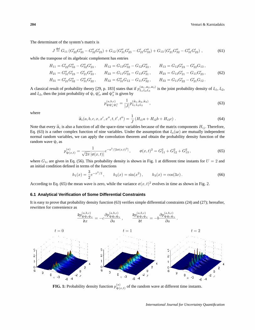
whereG1i are given in Eq. (56). This probability density is shown in Fig. 1 at different time instants forU = 2 andan initial condition defined in terms of the functions

h1(x) =32e−x2/2 , h2(x) = sin(x2) , h3(x) = cos(3x) . (66)

According to Eq. (65) the mean wave is zero, while the varianceσ(x, t)2 evolves in time as shown in Fig. 2.

6.1 Analytical Verification of Some Differential Constraints

It is easy to prove that probability density function (63) verifies simple differential constraints (24) and (27); hereafter,rewritten for convenience as

dp(a,b,c)ψψtψx

dx= −c

∂p(a,b,c)ψψtψx

∂a,

dp(a,b,c)ψψtψx

dt= −b

∂p(a,b,c)ψψtψx

∂a.

t = 0 t = 1 t = 2

FIG. 1: Probability density functionp(a)ψ(x,t) of the random wave at different time instants.



x

t

−4 −3 −2 −1 0 1 2 3 40

0.4

0.8

1.2

1.6

2

0

0.5

1

1.5

2

2.5

3

FIG. 2: Temporal evolution of the wave variance.

To this end, let us first notice that the limit partial derivatives of Jacobian determinant (61) with respect tox andt areidentically zero; i.e., we have

dJ

dx= 0 ,

dJ

dt= 0 . (67)

In fact, by using definitions (57) and (58) we obtain


∂J

∂x= G31 (G22G33 −G32G23) + G32 (G31G23 −G21G33) + G33 (G21G32 −G31G22) = 0 , (68)


∂J

∂t= G21 (G22G33 −G32G23) + G22 (G31G23 −G21G33) + G23 (G21G32 −G31G22) = 0 . (69)

At this point, we can calculate the limit derivatives of probability density (63) with respect tox andt:

dp(a,b,c)ψψtψx

dx= − 1

J |J |dJ

dxp(α1,α2,α3)ξ1ξ2ξ3

+1|J |

∂p(α1,α2,α3)ξ1ξ2ξ3

∂αi

dαi

dx=

1|J |

∂p(α1,α2,α3)ξ1ξ2ξ3

∂αi

dαi

dx, (70)

dp(a,b,c)ψψtψx

dt= − 1

J |J |dJ

dtp(α1,α2,α3)ξ1ξ2ξ3

+1|J |

∂p(α1,α2,α3)ξ1ξ2ξ3

∂αi

dαi

dt=

1|J |

∂p(α1,α2,α3)ξ1ξ2ξ3

∂αi

dαi

dt, (71)

where we have used Eqs. (67). From Eqs. (64) and (67) and definitions (57) and (58) it follows that

dαi

dx= − 1

JHi1c ,

dαi

dt= − 1

JHi1b . (72)

Substituting these results back into Eqs. (70) and (71) we obtain

dp(a,b,c)ψψtψx

dx= − c

J |J |∂p

(α1,α2,α3)ξ1ξ2ξ3

∂αiHi1 ,

dp(a,b,c)ψψtψx

dt= − b

J |J |∂p

(α1,α2,α3)ξ1ξ2ξ3

∂αiHi1 . (73)

At the same time we notice that

−c∂p

(a,b,c)ψψtψx

∂a= − c

J |J |∂p

(α1,α2,α3)ξ1ξ2ξ3

∂αi

∂αi

∂a= − c

J |J |∂p

(α1,α2,α3)ξ1ξ2ξ3

∂αiHi1 , (74)

−b∂p

(a,b,c)ψψtψx

∂a= − b

J |J |∂p

(α1,α2,α3)ξ1ξ2ξ3

∂αi

∂αi

∂a= − b

J |J |∂p

(α1,α2,α3)ξ1ξ2ξ3

∂αiHi1 , (75)



and, therefore, differential constraints (24) and (27) are satisfied identically [simply compare Eqs. (74) and (75) withEqs. (73)]. Similarly, it is possible to show analytically that higher-order constraints such as Eqs. (33), (12), or (31)are satisfied identically by joint probability density function (63). We conclude this section by emphasizing that thereexist many joint densities satisfying a single differential constraint [e.g., Eq. (12)], for the same boundary and initialconditions. As an example, simply consider the family of probability densities in the form of Eq. (63) where functionsαi are translated by rather arbitrary functionsχi(x′, x′′, t′, t′′) defined forx′, x′′ ∈ R, t′, t′′ ≥ t0 and satisfyingχi = 0 for t′ = t0 or t′′ = t0. This clearly shows that a boundary value problem for Eq. (12) alone is ill posed; i.e., itadmits an infinite number of solutions.

7. SUMMARY

We have determined and discussed new differential constraints satisfied by the joint probability density function ofarbitrary random waves governed by Eq. (1) for random boundary conditions and random initial conditions. Thesedifferential constraints involve unusual limit partial differential operators, and they can be classified into two maingroups: the first one depends on the stochastic wave equation while the second one includes a set of intrinsic relationsdetermined by the structure of the joint probability density function of the wave and its derivatives. We have shownthat in those cases where an evolution equation for the probability density function exists (e.g., for first-order nonlinearstochastic PDEs) the set of differential constraints is complete; i.e., it allows us to determine the probability densityfunction of the solution. We have applied the new theory to a random wave process in a one-dimensional spatialdomain and we have shown analytically that the differential constraints for the joint probability density functionare satisfied identically. In addition, we have argued that a boundary value problem involving only one differentialconstraint is, in general, not well posed; i.e., it admits an infinite number of solutions. This brings us back to thefundamental question we have addressed at the beginning of this paper: How many differential constraints do we needin order to have enough information to compute the probability density function of the system uniquely? Most likelythe full set of first-order differential constraints, which has been proven to be complete for first-order stochastic PDEs,is not sufficient and the full hierarchy of equations have to be considered (see, e.g., [40]). We conclude by emphasizingthat the sequence of steps that led us to formulate the set of differential constraints presented in this paper can berepeated with some modifications for other linear and nonlinear stochastic PDEs. In other words, we have provided ageneral methodology that allows us to obtain an ensemble of conditions, in the form of partial differential equations,for the probability density function of the solution to an arbitrary stochastic PDE.

ACKNOWLEDGMENTS

We acknowledge financial support from OSD-MURI Grant Number FA9550-09-1-0613, DOE Grant Number DE-FG02-07ER25818, and NSF Grant Number DMS-0915077.

REFERENCES

1. Ghanem, R. G. and Spanos, P. D.,Stochastic Finite Elements: A Spectral Approach, Springer, New York, 1998.

2. Xiu, D. and Karniadakis, G. E., The Wiener–Askey polynomial chaos for stochastic differential equations,SIAM J. Sci.Comput., 24(2):619–644, 2002.

3. Wan, X. and Karniadakis, G. E., Multi-element generalized polynomial chaos for arbitrary probability measures,SIAM J. Sci.Comput., 28(3):901–928, 2006.

4. Venturi, D., Wan, X., and Karniadakis, G. E., Stochastic bifurcation analysis of Rayleigh-Benard convection,J. Fluid. Mech.,650:391–413, 2010.

5. Foo, J. and Karniadakis, G. E., Multi-element probabilistic collocation method in high dimensions,J. Comput. Phys.,229:1536–1557, 2010.

6. Ma, X. and Zabaras, N., An adaptive hierarchical sparse grid collocation method for the solution of stochastic differentialequations,J. Comput. Phys., 228:3084–3113, 2009.



7. Nouy, A., Proper generalized decompositions and separated representations for the numerical solution of high dimensionalstochastic problems,Arch. Comput. Methods Appl. Mech. Eng., 17:403–434, 2010.

8. Nouy, A. and Maıtre, O. P. L., Generalized spectral decomposition for stochastic nonlinear problems,J. Comput. Phys.,228:202–235, 2009.

9. Venturi, D., On proper orthogonal decomposition of randomly perturbed fields with applications to flow past a cylinder andnatural convection over a horizontal plate,J. Fluid Mech., 559:215–254, 2006.

10. Venturi, D., Wan, X., and Karniadakis, G. E., Stochastic low-dimensional modelling of a random laminar wake past a circularcylinder,J. Fluid Mech., 606:339–367, 2008.

11. Venturi, D., A fully symmetric nonlinear biorthogonal decomposition theory for random fields,Physica D, 240(4-5):415–425,2010.

12. Martin, P. C., Siggia, E. D., and Rose, H. A., Statistical dynamics of classical systems,Phys. Rev. A, 8:423–437, 1973.

13. Jouvet, B. and Phythian, R., Quantum aspects of classical and statistical fields,Phys. Rev. A, 19:1350–1355, 1979.

14. Jensen, R. V., Functional integral approach to classical statistical dynamics,J. Stat. Phys., 25(2):183–210, 1981.

15. Phythian, R., The functional formalism of classical statistical dynamics,J. Phys. A: Math. Gen., 10(5):777–788, 1977.

16. Phythian, R., The operator formalism of classical statistical dynamics,J. Phys A: Math. Gen., 8(9):1423–1432, 1975.

17. Tennekes, H. and Lumley, J. L.,A First Course in Turbulence, MIT Press, Cambridge, MA, 1972.

18. Monin, A. S. and Yaglom, A. M.,Statistical Fluid Mechanics, vol. 1, Dover, New York, 2007.

19. Klyatskin, V. I., Dynamics of Stochastic Systems, Elsevier, Amsterdam, The Netherlands, 2005.

20. Sapsis, T. P. and Athanassoulis, G., New partial differential equations governing the response-excitation joint probabilitydistributions of nonlinear systems under general stochastic excitation,Prob. Eng. Mech., 23:289–306, 2008.

21. Bochkov, G. N. and Dubkov, A. A., Concerning the correlation analysis of nonlinear stochastic functionals,Radiophys. Quan-tum Electron., 17(3):288–292, 1974.

22. Bochkov, G. N., Dubkov, A. A., and Malakhov, A. N., Structure of the correlation dependence of nonlinear stochastic func-tionals,Radiophys. Quantum Electron., 20(3):276–280, 1977.

23. Hanggi, P., On derivations and solutions of master equations and asymptotic represenations,Z. Phys. B, 30:85–95, 1978.

24. Chen, H., Chen, S., and Kraichnan, R. H., Probability distribution of a stochastically advected scalar field,Phys. Rev. Lett.,63:2657–2660, 1989.

25. Pope, S. B., Mapping closures for turbulent mixing and reaction,Theor. Comput. Fluid Dyn., 2:255–270, 1991.

26. Kim, S. H., On the conditional variance and covariance equations for second-order conditional moment closure,Phys. Fluids,14(6):2011–2014, 2002.

27. Tartakovsky, D. M. and Broyda, S., PDF equations for advective-reactive transport in heterogeneous porous media with un-certain properties,J. Contam. Hydrol., 120-121:129–140, 2011.

28. Carrier, G. F. and Pearson, C. E.,Partial Differential Equations: Theory and Technique, Academic, New York, 1976.

29. Papoulis, A.,Probability, Random Variables and Stochastic Processes, 3rd ed., McGraw-Hill, New York, 1991.

30. Khuri, A. I., Applications of Dirac’s delta function in statistics,Int. J. Math. Educ. Sci. Technol., 35(2):185–195, 2004.

31. Kanwal, R. P.,Generalized Functions: Theory and Technique, 2nd ed., Birkhauser, Boston, 1998.

32. Rosen, G., Dynamics of probability distributions over classical fields,Int. J. Theor. Phys., 4(3):189–195, 1971.

33. Lewis, R. M. and Kraichnan, R. H., A space-time functional formalism for turbulence,Commun. Pure Appl. Math., 15:397–411, 1962.

34. Rosen, G.,Formulations of Classical and Quantum Dynamical Theory, vol. 60, Academic, New York, 1969.

35. Volterra, V.,Theory of Functionals and of Integral and Integro-Differential Equations, Dover, Mineola, NY, 1959.

36. Volterra, V.,Lecons sur les Fonctions de Ligne, Gauthier Villas, Paris, 1913.

37. Vainberg, M. M.,Variational Methods for the Study of Nonlinear Operators, Holden-Day, San Francisco, 1964.

38. Nashed, M. Z., Differentiability and related properties of non-linear operators: Some aspects of the role of differentials innon-linear functional analysis,Nonlinear Functional Analysis and Applications, Rall, L. B., ed., Academic, New York, 1971.

39. Tuckerman, M. E.,Statistical Mechanics: Theory and Molecular Simulation, Oxford University Press, Oxford, UK, 2010.



40. Lundgren, T. S., Distribution functions in the statistical theory of turbulence,Phys. Fluids, 10(5):969–975, 1967.

APPENDIX A. FUNCTIONAL REPRESENTATION OF THE PROBABILITY DENSITY FUNCTION OFTHE SOLUTION TO STOCHASTIC PDES

Let us consider a physical system described in terms of PDEs subject to uncertain initial conditions, boundary con-ditions, physical parameters, or external forcing terms. The solution to these types of boundary value problems is arandom field whose regularity properties in space and time are related strongly to the type of nonlinearities appearingin the equations as well as to the statistical properties of the random input processes. In this paper we assume that theprobability density function of the solution field exists. In order to fix ideas, let us consider the advection-diffusionequation

∂ψ

∂t+ ξ(ω)

∂ψ

∂x= ν

∂2ψ

∂x2, (A.1)

with deterministic boundary and initial conditions. The parameterξ(ω) is assumed to be a random variable withknown probability density function. The solution to Eq. (A.1) is a random field depending on the random variableξ(ω) in a possibly nonlinear way. We shall denote such a functional dependence asψ(x, t; [ξ]). The joint probabilitydensity ofψ(x, t; [ξ]) andξ [i.e., the solution field at the space-time location(x, t) and the random variableξ] admitsthe following integral representation (see Eq. (16) in [30]):

p(a,b)ψ(x,t)ξ = 〈δ(a−ψ(x, t; [ξ]))δ(b− ξ)〉 , a, b ∈ R . (A.2)

The average operator〈·〉, in this particular case, is defined as a simple integral with respect to the probability densityof ξ(ω); i.e.,

p(a,b)ψ(x,t)ξ =

∫ ∞

−∞δ[a−ψ(x, t; [z])]δ(b− z)p(z)

ξ dz , (A.3)

wherep(z)ξ denotes the probability density ofξ which could be compactly supported (e.g., a uniform distribution). The

support of the probability density functionp(a,b)ψ(x,t)ξ is determined by the nonlinear transformationξ → ψ(x, t; [ξ])

appearing within the delta functionδ[a − ψ(x, t; [ξ])] (see, e.g., Chap. 3 in [31]). Simple representation (A.3) canbe generalized easily to infinite dimensional random input processes. To this end, let us examine the case where thescalar fieldψ is advected by a random velocity fieldU according to the equation

∂ψ

∂t+ U(x, t; ω)

∂ψ

∂x= ν

∂2ψ

∂x2, (A.4)

for some deterministic initial condition and boundary conditions. Disregarding the particular form of the randomfield U(x, t; ω), let us consider its collocation representation for a given discretization of the space-time domain.This gives us a certain number of random variables{U(xi, tj ;ω)} (i = 1, .., N , j = 1, ..., M ). The random fieldψsolving Eq. (A.4) at each one of these locations is, in general, a nonlinear function of all the variables{U(xi, tj ; ω)}.In order to see this, it is sufficient to write an explicit finite-difference numerical scheme of Eq. (A.4). The jointprobability density of the solution fieldψ at (xi, tj) and the driving fieldU at (xn, tm), admits the following integralrepresentation:

p(a,b)ψ(xi,tj)U(xn,tm) = 〈δ{a−ψ(xi, tj ; [U(x1, t1), ..., U(xN , tM )])}δ[b− U(xn, tm)]〉 , (A.5)

where the average, in this case, is with respect to the joint probability of all the random variables{U(xn, tm; ω)}(n = 1, .., N , m = 1, ...,M ). The notationψ(xi, tj ; [U(x1, t1), ..., U(xN , tM )]) emphasizes that the solution fieldψ(xi, tj) is, in general, a nonlinear function of all the random variables{U(xn, tm; ω)}. If we send the number ofthese variables to infinity (i.e., we refine the space-time mesh to the continuum level), we obtain a functional integralrepresentation of the joint probability density



p(a,b)ψ(x,t)U(x′,t′) = 〈δ[a−ψ(x, t; [U ])]δ[b− U(x′, t′)]〉 =

∫D[U ]W [U ]δ[a−ψ(x, t; [U ])]δ[b− U(x′, t′)] , (A.6)

whereW [U ] is the probability density functional of random fieldU(x, t; ω) andD[U ] is the usual functional integralmeasure [13–15]. Depending on the particular equation of motion, we will need to consider different joint probabilitydensity functions; e.g., the joint probability of a field and its derivatives with respect to space variables. The functionalrepresentation described above allows us to deal with these different situations in a very practical way. For instance,the joint probability density of a fieldψ(x, y, t) and its first-order spatial derivatives at different space-time locationscan be represented as

p(a,b,c)ψ(x,y,t)ψx(x′,y′,t′)ψy(x′′,y′′,t′′) = 〈δ[a−ψ(x, y, t)]δ[b−ψx(x′, y′, t′)]δ[c−ψy(x′′, y′′, t′′)]〉 , (A.7)

where, for notational convenience, we have denoted byψxdef= ∂ψ/∂x, ψy

def= ∂ψ/∂y and we have omitted thefunctional dependence on the random input variables within each field. Similarly, the joint probability ofψ(x, y, t) attwo different spatial locations is

p(a,b)ψ(x,y,t)ψ(x′,y′,t) = 〈δ[a−ψ(x, y, t)]δ[b−ψ(x′, y′, t)]〉 . (A.8)

In order to lighten the notation further, sometimes we will drop the subscripts indicating the space-time variables andwrite, for instance

p(a,b)ψψ′x

= 〈δ[a−ψ(x, y, t)]δ[b−ψx(x′, y′, t′)]〉 , (A.9)

or even more compactly

p(a,b)ψψ′x

= 〈δ(a−ψ)δ(b−ψ′x)〉 . (A.10)

A.1 Representation of Derivatives

The differentiation of the probability density function with respect to space and time variables involves generalizedderivatives of the Dirac delta function and it can be carried out in a systematic manner. To this end, let us considerEq. (A.2) and define the following linear functional:

∫ ∞

−∞p(a)ψ(x,t)ρ(a)da =

⟨∫ ∞

−∞δ[a−ψ(x, t)]ρ(a)da

⟩= 〈ρ(ψ)〉 , (A.11)

whereρ(a) is a continuously differentiable and compactly supported function. A differentiation of Eq. (A.11) withrespect tot gives

∫ ∞

−∞

∂p(a)ψ(x,t)

∂tρ(a)da = 〈ψt

∂ρ

∂ψ〉 =

⟨ψt

∫ ∞

−∞

∂ρ

∂aδ[a−ψ(x, t)]da

⟩

=∫ ∞

−∞− ∂

∂a〈ψtδ[a−ψ(x, t)]〉ρ(a)da .

(A.12)

This equation holds for an arbitraryρ(a) and therefore we have the identity

∂p(a)ψ(x,t)

∂t= − ∂

∂a〈δ [a−ψ(x, t)] ψt(x, t)〉 . (A.13)

Similarly,

∂p(a)ψ(x,t)

∂x= − ∂

∂a〈δ [a−ψ(x, t)] ψx(x, t)〉 . (A.14)



Straightforward extensions of these results allow us to compute derivatives of joint probability density functionsinvolving more fields; e.g.,ψ(x, t) and its first-order spatial derivativeψx(x, t). For instance, we have

∂p(a,b)ψψx

∂t=− ∂

∂a〈δ [a−ψ(x, t)] δ[b−ψx(x, t)]ψt(x, t)〉− ∂

∂b〈δ [a−ψ(x, t)] δ[b−ψx(x, t)]ψtx(x, t)〉, (A.15)

whereψtxdef= ∂2ψ/∂t∂x.

A.2 Representation of Averages

In this section we determine important formulas to compute the average of a product between Dirac delta functionsand various fields. To this end, let us first consider the average〈δ(a − ψ)ψ〉. By applying well-known properties ofDirac delta functions it can be shown that

〈δ(a−ψ)ψ〉 = ap(a)ψ(x,t) . (A.16)

This result is a multidimensional extension of the following trivial identity that holds for one random variableξ (withprobability densityp(z)

ξ ) and a nonlinear functiong(ξ) (see, e.g., Ch. 3 of [31] or [30]):

∫ ∞

−∞δ[a− g(z)]g(z)p(z)

ξ dz =∑

n

1|g′(zn)|

∫ ∞

−∞δ(z − zn)g(z)p(z)

ξ dz =∑

n

g(zn)p(zn)ξ

|g′(zn)| , (A.17)

wherezn = g−1(a) are roots ofg(z) = a. Sinceg(zn) = g(g−1(a)) = a, from Eq. (A.17) it follows that

∫ ∞

−∞δ[a− g(z)]g(z)p(z)

ξ dz = a∑

n

p(zn)ξ

|g′(zn)| = a

∫ ∞

−∞δ(a− g(z))p(z)

ξ dz , (A.18)

which is the one-dimensional version of Eq. (A.16). Similarly, one can show that

〈δ(a−ψ)δ(b−ψx)ψ〉 = ap(a,b)ψψx

, (A.19)

〈δ(a−ψ)δ(b−ψx)ψx〉 = bp(a,b)ψψx

, (A.20)

and, more generally, that

〈δ(a−ψ)δ(b−ψx)h(x, t, ψ, ψx)〉 = h(x, t, a, b)p(a,b)ψψx

, (A.21)

where, for the purposes of the present paper,h(ψ,ψx, x, t) is any continuous function ofψ, ψx, x, andt. The result[Eq. (A.21)] can be generalized even further to averages involving a product of functions in the form

〈δ(a−ψ)δ(b−ψx)h(x, t, ψ,ψx)g(x, t, ψxx, ψxt, ψtt, ...)〉= h(x, t, a, b)〈δ(a−ψ)δ(b−ψx)g(x, t, ψxx, ψxt,ψtt, ...)〉 .

(A.22)

In short, the general rule is: we are allowed to take out of the average all those functions involving fields for whichwe have available a Dirac delta. As an example, ifψ is a time-dependent random field in a two-dimensional spatialdomain we have

〈δ(a−ψ)δ(b−ψx)δ(c−ψy)e−(x2+y2) sin(ψ)ψxψ2yψxx〉

= e−(x2+y2) sin(a)bc2〈δ(a−ψ)δ(b−ψx)δ(c−ψy)ψxx〉 .(A.23)



APPENDIX B. HOPF CHARACTERISTIC FUNCTIONAL APPROACH

In this appendix we employ a Hopf characteristic functional approach [19, 32–34] to derive the differential constraint(12) for the probability density function of one-dimensional random waves satisfying Eq. (2). This allows us to showhow the differential constraints for the probability density function can be obtained from general principles. The jointHopf characteristic functional of the waveψ and its derivatives with respect to space and time is defined as

F [α, β, γ] def= 〈eZ[α,β,γ]〉 , (B.1)

where

Z[α,β, γ] = i

∫

T

∫

X

ψ (X, τ;ω)α(X, τ)dXdτ + i

∫

T

∫

X

ψt (X, τ;ω)β(X, τ)dXdτ

+ i

∫

T

∫

X

ψx (X, τ; ω)γ(X, τ)dXdτ

(B.2)

and the average operator is a functional integral with respect to the joint probability functional of the random initialcondition and the random boundary conditions. The Volterra functional derivative [35, 36] of Eq. (B.1) with respect toψ(x, t); i.e., the Gateaux differential [37, 38] ofF [α,β, γ] with respect toα evaluated atz(X, t) = δ(t−τ)δ(x−X),is

δF [α, β, γ]δψ(x, t)

def= i〈ψ(x, t; ω)eZ[α,β,γ]〉 . (B.3)

Similarly, the functional derivatives of Eq. (B.1) with respect toψt(x, t) andψx(x, t) are

δF [α, β, γ]δψt(x, t)

= i〈ψt(x, t;ω)eZ[α,β,γ]〉 , (B.4)

δF [α, β, γ]δψx(x, t)

= i〈ψx(x, t; ω)eZ[α,β,γ]〉 . (B.5)

Note that, by construction,

∂

∂x

(δF [α, β,γ]δψ(x, t)

)=

δF [α, β, γ]δψx(x, t)

, and∂

∂t

(δF [α, β, γ]δψ(x, t)

)=

δF [α,β, γ]δψt(x, t)

. (B.6)

If we differentiate Eq. (B.3) twice with respect tot andx

∂2

∂t2


)= i〈ψtt(x, t; ω)eZ[α,β,γ]〉 , (B.7)

∂2

∂x2


)= i〈ψxx(x, t;ω)eZ[α,β,γ]〉 . (B.8)

and we take into account Eq. (2), we easily determine the following functional differential equation governing for thedynamics of the Hopf characteristic functional:

∂2

∂t2

(δF [α, β, γ]δψ(x, t)

)= U2 ∂2

∂x2

(δF [α,β, γ]δψ(x, t)

). (B.9)

We notice that up to this point we have made no use of the fieldsβ andγ appearing in Eq. (B.1). Indeed, we can safelysetβ = 0 andγ = 0 in Eqs. (B.2) and (B.1) and determine exactly the same evolution [Eq. (B.9)]. The need forβ

andγ clearly appears when one tries to extract a pointwise equation for the probability density function of the randomwave from Eq. (B.9). To this end, let us first remark that functional differential equation (B.9) holds for arbitrary testfunctionsα, β, andγ. In particular, it holds for

α+(X, τ) = aδ(t− τ)δ(x−X) , (B.10)



β+(X, τ) = bδ(t′ − τ)δ(x′ −X) , (B.11)

γ+(X, τ) = cδ(t′′ − τ)δ(x′′ −X) . (B.12)

An evaluation of Eq. (B.9) forα = α+, β = β+, andγ = γ+ yields the condition

i⟨[

ψtt(x, t; ω)− U2ψxx(x, t; ω)]eiψ(x,t;ω)a+iψt(x

′,t′;ω)b+iψx(x′′,t′′;ω)c⟩

= 0 . (B.13)

This condition is equivalent to a differential constraint involving the joint characteristic function of the wave and itsderivatives

φ(a,b,c)ψψ′xψ′′t

def= 〈eiψ(x,t;ω)a+iψt(x′,t′;ω)b+iψx(x′′,t′′;ω)c〉 , (B.14)

In order to see this, let us notice that

∂2φ(a,b,c)ψψ′xψ′′t

∂t2= ia〈ψtt(x, t;ω)eiψ(x,t;ω)a+iψt(x

′,t′;ω)b+iψx(x′′,t′′;ω)c〉− a2〈ψt(x, t;ω)2eiψ(x,t;ω)a+iψt(x

′,t′;ω)b+iψx(x′′,t′′;ω)c〉 .(B.15)

If we take the limit of this expression for(t′, t′′) → t and(x′, x′′) → x we obtain

d2φ(a,b,c)ψψxψt

dt2= ia〈ψtt(x, t;ω)eiψ(x,t;ω)a+iψt(x,t;ω)b+iψx(x,t;ω)c〉+ a2

∂2φ(a,b,c)ψψxψt

∂b2, (B.16)

whered denotes the limit partial derivative operator. Similarly,

d2φ(a,b,c)ψψxψt

dx2= ia〈ψxx(x, t;ω)eiψ(x,t;ω)a+iψx(x,t;ω)b+iψt(x,t;ω)c〉+ a2


∂c2. (B.17)

At this point we can combine the results above to obtain the following differential constraint for the joint characteristicfunction:

d2φ(a,b,c)ψψxψt

dt2− a2


∂b2= U2

d2φ(a,b,c)ψψxψt

dx2− U2a2


∂c2. (B.18)

The inverse Fourier transform of this relation with respect toa, b, andc gives us exactly Eq. (12). In order to provethis, we simply recall the definition ofp(a,b,c)

ψψxψtas the inverse Fourier transform of the characteristic functionφ

(a,b,c)ψψxψt

:

p(a,b,c)ψψxψt

=1

(2π)3

∫ ∞

−∞

∫ ∞

−∞

∫ ∞

−∞e−iaα−ibβ−icηφ

(α,β,η)ψψxψt

dαdβdη , (B.19)

and two simple relations arising from Fourier transformation theory of a one dimensional functionf(x):∫ ∞

−∞e−iax dnf(x)

dxndx = (ia)n

∫ ∞

−∞e−iaxf(x)dx , (B.20)

∫ ∞

−∞e−iaxxnf(x)dx = in

dn

dan

∫ ∞

−∞e−iaxf(x)dx . (B.21)

APPENDIX C. PERTURBATION EXPANSIONS OF DIFFERENTIAL CONSTRAINTS

In this appendix we show that differential constraint (12) can be expanded in a perturbation series leading to anequation governing the local behavior of the probability density function in the neighborhood of the hyperplanex′′ = x′ = x, t′′ = t′ = t. To this end, let us consider again Eq. (8):


∂t2− U2


∂x2=

∂2

∂a2〈δ (a−ψ)ψ2

t δ (b−ψ′t) δ (c−ψ′′x)〉

+U∂2

∂a2〈δ (a−ψ)ψ2

xδ (b−ψ′t) δ (c−ψ′′x)〉(C.1)



and look for an approximation to both averages appearing on the right-hand side. The simplest one consists in ex-pandingψ2

t andψ2x in a first-order Taylor series around(x′, t′) and(x′′, t′′), respectively; i.e.,

ψ2t = ψ′2t + 2ψ′tψ

′tx(x− x′) + 2ψ′tψ

′tt(t− t′) + · · · , (C.2)

ψ2x = ψ′′2x + 2ψ′′xψ′′xx(x− x′′) + 2ψ′′xψ′′xt(t− t′′) + · · · . (C.3)

A substitution of Eqs. (C.2) and (C.3) into the averages in Eq. (C.1) yields

〈δ (a−ψ) ψ2t δ (b−ψ′t) δ (c−ψ′′x)〉 = 〈δ (a−ψ) ψ′2t δ (b−ψ′t) δ (c−ψ′′x)〉

+2(x− x′)〈δ (a−ψ)ψ′tψ′txδ (b−ψ′t) δ (c−ψ′′x)〉+ 2(t− t′)〈δ (a−ψ)ψ′tψ

′ttδ (b−ψ′t) δ (c−ψ′′x)〉 ,

(C.4)

〈δ (a−ψ) ψ2xδ (b−ψ′t) δ (c−ψ′′x)〉 = 〈δ (a−ψ) ψ′′2x δ (b−ψ′t) δ (c−ψ′′x)〉

+2(x−x′′)〈δ (a−ψ)ψ′′xψ′′xxδ (b−ψ′t) δ (c−ψ′′x)〉+2(t− t′′)〈δ (a−ψ)ψ′′xψ′′xtδ (b−ψ′t) δ (c−ψ′′x)〉 .(C.5)

At this point we can use property (A.22) and write Eqs. (C.4) and (C.5) as

〈δ (a−ψ) ψ2t δ (b−ψ′t) δ (c−ψ′′x)〉= b2p

(a,b,c)ψψ′tψ′′x

+ 2b(x− x′)∫ b

−∞

∂p(a,b′,c)ψψ′tψ′′x

∂x′db′

+2b(t− t′)∫ b

−∞

∂p(a,b′,c)ψψ′tψ′′x

∂t′db′ ,

(C.6)

〈δ (a−ψ)ψ2xδ (b−ψ′t) δ (c−ψ′′x)〉= c2p

(a,b,c)ψψ′tψ′′x

+ 2c(x− x′′)∫ c

−∞

∂p(a,b,c′)ψψ′tψ′′x

∂x′′dc′

+2c(t− t′′)∫ c

−∞

∂p(a,b,c′)ψψ′tψ′′x

∂t′′dc′ .

(C.7)

A substitution of Eqs. (C.6) and (C.7) into Eq. (C.1) yields a fourth-order (nine-dimensional) partial differentialequation that characterizes locally; i.e., in the neighborhood of the hyperplanex = x′ = x′′, t = t′ = t′′ the evolutionof the probability density function of the random wave. Equivalently, we can say that we have determined a local(non-pointwise) realization of functional differential Eq. (B.9). An alternative method to obtain this result consists inevaluating functional differential Eq. (B.9) for test functionsα, β, andγ that are very concentrated near specific space-time locations. These types of test functions can be any of those belonging to a delta sequence (see, e.g., Appendix Ain [39]).


differential constraints for the probability … · density function of stochastic solutions to the...

Documents