differential registration bias in voter file data: a …nyhan/diff-reg-bias.pdfdifferential...

Differential Registration Bias in Voter File Data:A Sensitivity Analysis Approach⇤

Brendan NyhanProfessor

Dept. of GovernmentDartmouth CollegeHinman Box 6108

305 Silsby HallHanover, NH 03755

[email protected]

Christopher SkovronPh.D. Candidate

Dept. of Political ScienceUniversity of Michigan

5700 Haven Hall505 South State StreetAnn Arbor, MI 48109

[email protected]

Rocı́o TitiunikJames Orin Murfin Associate Professor

Dept. of Political ScienceUniversity of Michigan

5700 Haven Hall505 South State StreetAnn Arbor, MI 48109

[email protected]

Short title: Differential Registration Bias in Voter File Data

Keywords: Voter file, voter turnout, post-treatment bias, selection bias

⇤We thank Matias Cattaneo, Alexander Coppock, Simon Chauchard, Kevin Collins, Jeff Friedman, Brian Greenhill,Michael Herron, Yusaku Horiuchi, Jeremy Horowitz, Dean Lacy, Jacob Montgomery, Phil Paolino, Jason Reifler,Daniel Smith, Brad Spahn, Thomas Zeitzoff, seminar participants at the UCLA American Politics Workshop andthe UC-Davis Political Science Speaker Series, the editor, and three anonymous reviewers for helpful feedback; BobBlaemire at Catalist for his assistance in procuring our data; and John Holbein and Sunshine Hillygus for providingreplication data. All errors are our own. Nyhan acknowledges support from the Robert Wood Johnson Foundation’sScholars in Health Research Program. Skovron acknowledges funding from the NSF Graduate Research FellowshipProgram. Titiunik acknowledges financial support from the National Science Foundation (SES 1357561).

Abstract

The widespread availability of voter files has improved the study of participation in Americanpolitics, but the lack of comprehensive data on non-registrants creates difficult inferential is-sues. Most notably, observational studies that examine turnout rates among registrants oftenimplicitly condition on registration, a post-treatment variable that can induce bias if the treat-ment of interest also affects the likelihood of registration. We introduce a sensitivity analysisto assess the potential bias induced by this problem, which we call differential registrationbias. Our approach is most helpful for studies that estimate turnout among registrants usingpost-treatment registration data, but is also valuable for studies that estimate turnout amongthe voting-eligible population using secondary sources. We illustrate our approach with twostudies of voting eligibility effects on subsequent turnout among young voters. In both cases,eligibility appears to decrease turnout, but these effects are found to be highly sensitive todifferential registration bias.

Replication materials: The data, code, and any additional materials required to replicate allanalyses in this article are available on the American Journal of Political Science Dataversewithin the Harvard Dataverse Network at http://dx.doi.org/10.7910/DVN/LCDBRU.

Word count: 8,968

The widespread availability of digital voter files has changed the study of voting behavior in Amer-

ican politics. These files offer data on a vast population of U.S. citizens while avoiding the social

desirability bias and low statistical power that plague survey studies of self-reported turnout, en-

abling new studies of how factors as disparate as majority-minority districts (Barreto, Segura and

Woods 2004), minority candidates (Barreto 2007; Fraga 2016a), genetic similarity (Fowler, Baker

and Dawes 2008), and early voting registration (Holbein and Hillygus 2015) affect turnout at the

individual or aggregate level. These data have been found to be of high quality, especially when

cleaned and aggregated by firms like Catalist (Ansolabehere and Hersh 2012; Hersh 2015).

However, greater attention is needed to the limitations of these data sources. Ideally, the de-

nominator for turnout studies should be the voting-eligible population (VEP). Unfortunately, a lack

of precise data on the VEP makes turnout estimates vulnerable to estimation error (e.g., McDonald

and Popkin 2001). In the U.S., common choices to approximate the VEP are the voting-age pop-

ulation (VAP) or the citizen voting-age population (CVAP), but these measures are imperfect ap-

proximations: both include ineligible populations such as disenfranchised felons; the VAP includes

noncitizens; and the CVAP is estimated based on surveys—not census counts—and is unavailable

for the smallest census geographies.

As a result, researchers often estimate turnout effects using voter registration files, which can

take at least two different forms. In what we call pre-treatment registrant studies, scholars study a

subset of citizens to whom a treatment of interest is assigned (or not) after they have registered to

vote. These studies can be either experimental or non-experimental. For example, studies of get-

out-the-vote (GOTV) campaigns typically start with a list of registered voters, randomly assign

each citizen in the list to be encouraged to vote (or not), and use future voter files to measure

subsequent turnout (e.g., Gerber, Green and Larimer 2008; Citrin, Green and Levy 2014). Other

studies identify the period when a non-experimental intervention or treatment is introduced, collect

registration files from a period before treatment, and look at the effect of the treatment on the

subpopulation of registrants identified before the treatment (e.g., Barber and Imai 2014; Enos 2016;

Fraga 2016b). The common feature of this type of studies is that the registration decisions that

1

determine the study population occur before the treatment is assigned.1

In contrast, in what we call post-treatment registrant studies, researchers are typically interested

in the effect of a non-experimental treatment on voter turnout (or partisan registration) and use voter

registration files as the source of outcome data without limiting the sample to registrants prior to

treatment. In these studies, the treatment of interest may affect both the likelihood of registration

and the likelihood of turning out to vote (or the likelihood of choosing to register as a partisan).

For example, the presence of a minority candidate on the ballot could lead to higher minority

registration as well as higher minority turnout, which will bias estimates of the effect of co-ethnic

candidates on turnout that are calculated among registrants.

Although both types of studies rely on registration files, they differ crucially in their study

populations. Pre-treatment registrant studies consider an initial group of registrants that is defined

and observed before the treatment is assigned. In contrast, post-treatment registrant studies con-

sider treatments that could affect both registration and voter turnout decisions while relying on

post-treatment registration files. In the latter studies, the decision to register may be a consequence

of the treatment itself, creating the potential for a form of post-treatment bias (Rosenbaum 1984)

sometimes known as “endogenous selection bias” (Elwert and Winship 2014). If a treatment affects

registration rates as well as voter turnout (the outcome of interest), a comparison of turnout rates

between the treated and control groups among registered voters could lead to mistaken inferences.

We formally show the threat that conditioning on the population of post-treatment registrants

poses in studies where the treatment of interest affects the likelihood of registration, characterizing

the bias that stems from differential registration in treated and control groups. We also develop a

novel sensitivity analysis that makes it possible for scholars to assess the robustness of their treat-

ment effect estimates to (unobserved) potential differences in registration rates between treatment

and control groups.

Our survey of the literature showed that most post-treatment registrant studies adopt one of

two strategies. Some studies, which are typically cross-sectional, simply use the registration file

as the universe of analysis and calculate turnout or partisanship rates as the proportion of voters1This characterization of pre-treatment registrant studies implicitly assumes that all subjects registered pre-

treatment remain registered or at least that the treatment has no effect on the probability of remaining registered.We do not pursue this issue further, but note that the sensitivity analysis we introduce could be appropriately modifiedto asses the robustness of results in cases where this assumption is violated.

2

or partisans among registrants (e.g., Barreto, Segura and Woods 2004; Barreto 2007; Fraga and

Merseth 2016; Hersh 2013; Hersh and Nall 2015). Other studies rely on voter files to calculate the

numerator of interest (number of voters or partisans), but calculate turnout or partisanship rates

using a measure of the potential electorate obtained from a secondary source as the denominator

(Meredith 2009; Fraga 2016a; Cepaluni and Hidalgo 2016).

The sensitivity approach we propose is useful in both cases. When the only data available is a

post-treatment cross-section of registered citizens, estimated treatment effects on turnout or parti-

sanship can be severely biased by differential registration between treatment and control groups.

Our approach offers a concrete measure of the robustness of treatment effects that are estimated in

this way. Our method is also useful for analyzing the robustness of estimates in which a secondary

source is used to calculate the denominator of turnout (or partisanship) rates. In these cases, our

approach can determine whether differential registration that would change the study’s conclusion

is within the plausible margin of error of the measure used to approximate the VEP.

We illustrate the challenge of differential registration and our sensitivity approach with two

studies of political socialization, a research area that has recently begun to use quasi-experimental

techniques to estimate the effect of initial election eligibility on subsequent voter turnout and other

behaviors (e.g., Meredith 2009; Mullainathan and Washington 2009; Dinas 2012, 2014; Coppock

and Green 2015; Holbein and Hillygus 2015). These studies typically compare voter turnout and

political attitudes among individuals whose 18th birthday fell close to a previous general election.

We use a similar research design that compares turnout rates between young citizens who were

narrowly eligible or ineligible to vote in a prior election.

Our first study is an original analysis of a sample of registrants from 42 U.S. states and the Dis-

trict of Columbia who were born within four days of the election eligibility cutoff—a far narrower

window than previous studies. Our findings illustrate the need to consider the potential bias induced

by conditioning on registration. When we naı̈vely use registered voters in the voter file as the de-

nominator for our turnout analysis, we find results that largely contradict previous studies—initial

election eligibility appears to sometimes reduce subsequent turnout or have no effect. However, we

show that this result is highly sensitive to differing registration rates between the two groups. Con-

sistent with this sensitivity analysis, when we instead use birth totals as the denominator, we find

3

that initial eligibility increases subsequent turnout. This application shows that differential regis-

tration between treatment and control groups can severely bias non-experimental turnout studies

when turnout rates are calculated as a proportion of total registration.

Our second study is a re-analysis of the Florida voter file findings in Holbein and Hillygus

(2015), where we again examine the effect of voting eligibility on subsequent turnout. Like the

first study, eligibility is found to negatively affect turnout in later elections among young voters

when turnout rates are calculated among registered voters. However, a sensitivity analysis of the

data indicates that even a slightly higher registration rate in the treatment group would reverse

these results. When we use birth counts to approximate the total population, we find that the reg-

istration rate is higher in the control group than in the treatment group in the window around the

eligibility cutoff originally used by Holbein and Hillygus, but this finding is reversed when a larger

window is considered. Our analysis suggests that the negative effects they report for the Florida

voter file are potentially sensitive to differential registration and could be consistent with true null

or even positive effects. This case illustrates the usefulness of our sensitivity method in cases where

approximations of the voting eligible population are imperfect.

These results suggest that scholars who study turnout based on voter files should complement

their analysis with a rigorous sensitivity analysis—even small differences in registration rates be-

tween treatment and control groups can reverse the conclusions of turnout studies. Our goal is not

to claim that past or current studies based on voter files are incorrect or misleading, but instead

to help raise awareness of this difficult inferential issue and provide researchers with a simple

approach to assess the robustness of their findings.

Defining and assessing differential registration bias

We begin by illustrating the problem of differential registration bias in Table 1 with a hypotheti-

cal example of an election in which 10,000 voting-eligible citizens are in the treatment group and

10,000 voting-eligible citizens are in the control group. In addition, the treatment is associated with

higher rates of registration—5,000 individuals in the treatment group register compared with 4,000

in the control group (column 2)—but has no effect on turnout (columns 3 and 5). If we simply com-

4

pare turnout rates among registered voters using voter file data (column 4), we would conclude that

turnout rates are lower among treated voters (2500/5000=50% versus 2500/4000=62.5% among

controls). However, the true turnout rate of 25% is identical in both groups (column 5).

[Table 1 about here.]

This problem would of course be avoided if we could calculate turnout rates using the total

voting-eligible population in each group rather than the total number of registered voters. When

possible, the simplest solution to the problem of differential registration is to obtain the missing

population totals from alternative data sources. However, as we discussed above, the necessary

data is typically either unavailable or imperfectly approximated.

A formal sensitivity analysis approach

We formalize a sensitivity analysis approach that can be implemented in cases where the needed

quantities—the total eligible population in the treatment and control groups—are unknown or im-

precisely estimated. Specifically, our approach identifies the differential in registration rates be-

tween the treatment and control groups that would reduce the observed difference in turnout rates

among registered voters to zero. This method provides a measure of the vulnerability of a treatment

effect estimate to differential registration bias when population totals are missing. It can also be

used to corroborate findings when population totals from alternative data sources are likely to be es-

timated with error, which is a pervasive phenomenon because precise counts of the voting-eligible

population are not directly available (McDonald and Popkin 2001). Moreover, as we discuss in the

conclusion and elaborate in the Supplemental Information, our approach could also be extended

to other types of data that share the characteristics of turnout data (unknown population totals and

values of missing data known with certainty).

In the example in Table 1, we assumed that all variables were known. We now assume that

total eligible population counts for the treatment and control groups are not available and that

researchers are working with a voter file that includes only registered voters.2 This scenario is il-

lustrated in Table 2, which presents the total number of registrants (column 2) and voters (column2For simplicity, we assume the entire registration file is available. However, our argument applies directly to the

case where only a random sample from the voter file is available (as in Study 1 below).

5

3) for each group, which allows us to calculate turnout rates among registrants by group (column

4). However, letting the subscripts T and C denote the treatment and control groups, respectively,

the total eligible population counts in each group, which we denote by PT

and PC

, respectively, are

not available. As a consequence, the true turnout rates—the ratio of voters to the total eligible pop-

ulation in each group—are also unavailable, creating the risk of a mistaken inference if differential

registration bias is present.


We introduce some additional notation. We let RT

and RC

denote the total registration counts

in the treatment and control groups, respectively, and VT

and VC

denote the total numbers of voters

who turned out to vote in each group. The desired—but unavailable—turnout rates are thus

T Pop

T

=VT

PT

and T Pop

C

=VC

PC

,

where the superscript Pop denotes that these turnout rates are calculated as a proportion of the total

(eligible) population. Henceforth, we refer to T Pop

T

and T Pop

C

as the turnout-to-population rates or

simply the true turnout rates. Without observing the eligible population counts PT

and PC

, we

cannot calculate these turnout-to-population rates directly.

We define the registration rates rT

= RT

/PT

and rC

= RC

/PC

in the treatment and control

groups, respectively. Given these rates, the total registration counts, RT

and RC

, can be expressed

as RT

= rT

⇥ PT

and RC

= rC

⇥ PC

, and we can express the unknown total eligible population as

total registration divided by the probability of registration:

PT

= RT

/rT

and PC

= RC

/rC

.

We then define the turnout-to-registration rate in each group, T Reg

T

and T Reg

C

, as follows:

T Reg

T

=VT

RT

and T Reg

C

=VC

RC

.

6

Given these definitions, we can express the desired turnout-to-population rates as

T Pop

T

=VT

PT

=VT

RT

/rT

= T Reg

T

⇥ rT

and T Pop

C

=VC

PC

=VC

RC

/rC

= T Reg

C

⇥ rC

. (1)

In words, the true turnout rate is the turnout-to-registration rate adjusted (multiplied) by the reg-

istration rate in each group. In applications where researchers have access to the voter file but not

the total population, the registration rates rT

and rC

are unknown. Our sensitivity analysis considers

how large the difference between rT

and rC

would have to be to generate the observed difference

in turnout-to-registration rates when the true difference in turnout-to-population rates is zero.

Imagine that T Reg

T

< T Reg

C

, which means that the turnout-to-registration rate is smaller in the

treatment than in the control group (as in the two applications we consider below). Because the

registration rates for the two groups rT

and rC

are unknown, T Reg

T

< T Reg

C

is not enough to conclude

that T Pop

T

< T Pop

C

.3 In other words, a lower (higher) turnout-to-registration rate in the treatment

group does not necessarily imply that this group has a lower (higher) turnout-to-population rate.

However, given the observed difference T Reg

T

�T Reg

C

, we can estimate how different the registration

rates would have to be between the treatment and the control groups for this difference to be

observed when there is no difference in turnout-to-population rates (i.e., when T Pop

T

� T Pop

C

= 0).

We define � as the treatment-control difference in true turnout rates:

� = T Pop

T

� T Pop

C

= (T Reg

T

⇥ rT

)� (T Reg

C

⇥ rC

).

We note two points. First, if rT

= rC

= 1, the expression simplifies to � = T Reg

T

� T Reg

C

. In other

words, if everyone in the treatment and control groups registers, the ratio of voters to registrants is

of course identical to the ratio of voters to total eligible population and there are no complications.

Second, if turnout rates are identical between groups but not everyone votes (rT

= rC

= r 6= 1),

the unknown turnout share difference simplifies to � = r(T Reg

T

� T Reg

C

). Since 0 r 1, in this

case the sign of � is equal to the sign of T Reg

T

� T Reg

C

and |�| |T Reg

T

� T Reg

C

|; moreover, it is

straightforward to explore how � changes as r varies from 0 to 1.

We are interested in the more general case in which both rT

and rC

are nonzero and rT

6=3Likewise, we cannot conclude that T Pop

T

> T Pop

C

or T Pop

C

= T Pop

T

without knowing rT

and rC

.

7

rC

. Figure 1 illustrates how a negative “treatment effect” on turnout-to-registration rates can be

observed even when the true difference in the turnout-to-population rates is null or even positive.

Using the functions defined in Equation (1), the figure plots the turnout-to-population rates (T Pop

T

,

T Pop

C

) against the registration rates (rT

, rC

) separately for each group, holding turnout-to-registration

rates (T Reg

T

, T Reg

C

) fixed. We adopt the scenario in Tables 1 and 2 where T Reg

T

= 0.50 and T Reg

C

=

0.625. Thus, we plot the linear functions T Pop

T

= 0.50⇥ rT

and T Pop

C

= 0.625⇥ rC

. Since the slope

in the control group (0.625) is higher than the slope in the treatment group (0.50), the dotted line

(control) is always above the solid line (treatment). In other words, Figure 1 fixes T Reg

C

= 0.50 and

T Reg

C

= 0.625, which means that the turnout-to-registration difference is always negative (-0.125).

[Figure 1 about here.]

Imagine first that the probability of registration in the treatment group is 0.8 (rT

= 0.8) and the

probability of registration in the control group is 0.4 (rC

= 0.4). In this case, the true turnout rate

in the treatment group (T Pop

T

) of 0.4 is obtained from the y-coordinate of point A on the solid line

in Figure 1(a), and the true turnout rate of 0.25 in the control group (T Pop

C

) is obtained from the y-

coordinate of point B on the dashed line. Under this scenario, � = T Pop

T

�T Pop

C

= 0.4�0.25 = 0.15.

In other words, the treatment effect on the true turnout-to-population rate is positive despite the

turnout-to-registration rate being lower in the treatment than in the control group. Figure 1(b)

shows a different scenario in which rT

= 0.8 and rC

= 0.64. In this case, both T Pop

T

and T Pop

C

are

equal to 0.4 and thus � = 0.4 � 0.4 = 0, though the difference in turnout-to-registration rates is

still negative (again, treatment slope is 0.5 and control slope is 0.625).

We propose a sensitivity analysis to explore how inferences are affected by differential regis-

tration. First, we define the differential registration factor k as the ratio of the registration rate in

the treatment group to the registration rate in the control group:

k =rT

rC

We assume that both rT

and rC

are nonzero. Moreover, because rT

and rC

are rates or probabilities,

they are both less than (or at most equal to) 1, which means that k 2 (0,1). Furthermore, since

rT

/k = rC

and rC

is a rate, k must satisfy the restriction 0 < rT

/k 1; that is, the smallest value

8

that k can take is rT

.4 Our sensitivity analysis explores, for a given treatment group registration rate

rT

, how large the differential registration factor k can be before the implied difference in turnout-

to-population rates is zero or has the opposite sign from T Reg

T

� T Reg

C

, the observed difference in

turnout-to-registration rates.

Given our definition of k, we can express �, the treatment-control difference in true turnout

rates, as a function of the treatment group registration rate rT

and the ratio of treatment/control

registration rates k:

�(rT

, k) = (T Reg

T

⇥ rT

)� (T Reg

C

⇥ rT

k) = r

T

(T Reg

T

� T Reg

C

k)

where we make the arguments k and rT

explicit. Thus, for any nonzero value of rT

, we can calculate

the value of k under which a zero difference in true turnout rates between the treatment and control

groups would result in the observed difference in turnout-to-registration rates. Since we assume

rT

> 0, we find this value, which we call k?, as the solution to (T Reg

T

� T Reg

C

k? ) = 0, leading to

k? =T Reg

C

T Reg

T

.

By definition, �(rT

, k?) = 0 for any 0 < rT

1.

We can now explore how the true turnout difference � varies with observed turnout-to-registration

rates under different assumptions about registration rates in the treatment and control groups (rT

and rC

). In particular, we can calculate k?, the pattern of differential registration that would be re-

quired to produce the observed difference in turnout-to-registration rates if there were no difference

in turnout-to-population rates.

We again illustrate the procedure with the hypothetical example presented in Tables 1 and 2.

In that example, T Reg

T

= 2500/5000 = 0.5 and T Reg

C

= 2500/4000 = 0.625, so the difference

in turnout rates among registered voters is negative (T Reg

T

� T Reg

C

= �0.125). In this case, k? =

0.625/0.50 = 1.25, which means that the observed difference in turnout-to-registration rates could

occur under a zero (or positive) difference in true turnout rates if the probability of registration

were (more than) 25% higher in the treatment than in the control group.4In other words, values of k 2 [0, r

T

) are not allowed because they would imply rC

� 1.

9

Figure 2 visualizes how the true turnout difference can vary with k—the ratio of the treat-

ment/control registration rates—for a given difference in turnout-to-registration rates. We plot

�(rT

, k) as a function of rT

for differing values of k (which implicitly fixes rC

). The y-axis is the

difference in turnout-to-population rates between the treatment and control groups and the x-axis

is the registration rate in the treatment group. As illustrated by the k? curve, when k = k? = 1.25,

the difference in true turnout rates is zero for every value of rT

. In contrast, when the registration

rate is equal in both groups and thus k = 1, the observed difference in turnout-to-registration rates

(T Reg

T

� T Reg

C

= �0.125) is equal to the true difference in turnout rates if rT

= 1.


We can explore sensitivity further in our hypothetical example by calculating the turnout rate

difference � for values of the registration ratio k above and below the threshold k?. For k >

k? = 1.25, the difference in true turnout is positive and the sign of the turnout-to-registration rate

difference is reversed. For 1 k < k? = 1.25, the true turnout effect is negative but smaller in

absolute value than the difference in turnout-to-registration rates for all rT

. Finally, for k < 1, the

true turnout effect is negative and can be larger in absolute value than the difference in turnout-to-

registration rates for a high enough rT

.

Incorporating prior knowledge of differential registration

The above approach allows researchers to assess a worst-case scenario in which differential regis-

tration bias produces the observed difference in turnout-to-registration rates when the true turnout-

to-population effect is zero. However, in some applications, the value taken by k? may not be

plausible or informative. We now describe a variant of this approach in which scholars can incor-

porate prior knowledge about plausible variation in registration rates in assessing the conditions

under which their results will hold.

Although the registration rates rT

and rC

are unknown, scholars often have prior information

about the range of plausible values they can take. Imagine that we use a survey estimate of the regis-

tration rate in the overall U.S. population as a guess for rT

, the true registration rate in the treatment

group. We call this guess r̃T

. Our concern is that rT

differs from rC

—i.e., that the treatment has an

10

effect on registration. In most cases, researchers will be able to offer some prior knowledge about

how large the differential registration effect is likely to be and rule out extreme values of k = rT

/rC

.

Imagine that our guess for the differential registration factor is k̃. We can use r̃T

and k̃ to calculate

the guessed treatment-control difference in true turnout rates, �̃ = r̃T

(T Reg

T

�T Reg

C

/k̃). If �̃ is of the

same sign as T Reg

T

� T Reg

C

, we can conclude the that observed difference in turnout-to-registration

rates is robust to a plausible scenario of differential registration rates based on prior knowledge

(which might be less stringent than the worst-case scenario represented by k?).

Consider our example above in which T Reg

T

= 0.50 and T Reg

C

= 0.625. Let us assume that our

guess for r̃T

is 0.59, the rate of registration in the overall U.S. population estimated by the Current

Population Survey in November 2014. Imagine that, based on prior knowledge, we believe that the

treatment of interest is unlikely to increase the registration rate in the treatment group by more than

ten percentage points relative to the control group. Since r̃T

= 0.59, our guess for rC

is about 0.49.

This yields k̃ = 0.59/0.49 = 1.20, which is less than k? = 1.25 and is therefore consistent with

a true negative small effect (�̃ = 0.59 · (0.50 � 0.625/1.20) = �0.012). In this way, our simple

sensitivity analysis approach can also be used to estimate whether an effect is robust to a particular

differential rate of registration chosen using prior knowledge.

Application: The effects of election eligibility on subsequent turnout

We now illustrate the problem of differential registration bias and our approach with two empirical

studies of political socialization that focus on the relationship between voting eligibility and sub-

sequent voter turnout. In Study 1, we present an original analysis of voter file data from 42 states.

In Study 2, we replicate results from a Florida voter file study in a recent article by Holbein and

Hillygus (2015).

Research in political socialization has found long-lasting effects of early experiences and events

like parent socialization (e.g., Jennings, Stoker and Bowers 2009) and draft status during the Viet-

nam War (Erikson and Stoker 2011). The most common and important socializing events for many

people as they approach or enter adulthood are elections—the time when politics is most salient in

national life. Sears and Valentino (1997), for instance, find that presidential elections appear to be

11

especially potent in forming the political views of adolescents.

These topics are the focus of an emerging literature that studies the effects of initial election

eligibility on voter turnout and other political behaviors using a quasi-experimental approach based

on voting-age eligibility rules (e.g., Coppock and Green 2015; Dinas 2012, 2014; Holbein and

Hillygus 2015; Meredith 2009; Mullainathan and Washington 2009). By comparing later turnout

and political attitudes among voters whose 18th birthday fell very close to a general election, these

studies seek to leverage as-if random variation in birth timing to compare individuals who had

the opportunity to take part in an election and those who did not but are assumed to be otherwise

identical. This research strategy is an application of a regression discontinuity (RD) design, which

we review below. We note, however, that these applications are only illustrations; our approach is

general and can be used in all turnout studies based on registration files, not just RD designs.

Studying eligibility effects with a regression discontinuity design

The defining feature of a (sharp) RD design is that subjects are assigned a score and receive treat-

ment if their score exceeds a known cutoff—and do not receive it otherwise. In the U.S., a discon-

tinuity in voting eligibility occurs when citizens turn eighteen years of age. As a result of the 26th

Amendment to the U.S. Constitution (adopted in 1971), people who turn eighteen on or before

election day can cast a vote but those who will turn eighteen after election day are ineligible to

vote. Thus, date of birth exactly determines voting eligibility and an RD design can be used to

study the effects of eligibility on turnout.

An important feature distinguishing RD designs based on date of birth from most uses of RD

is that the score that determines treatment, birthdate, is a discrete variable, which invalidates most

identification and estimation results in the RD literature. To address this issue, we adopt the frame-

work in Cattaneo, Frandsen and Titiunik (2015), which analyzes the RD design as a local random-

ized experiment in a fixed window around the cutoff and does not require a continuous running

variable.5 In our context, this randomization-based RD approach entails assuming that voting eli-

gibility is as-if randomly assigned for people with birthdays near election day. Since the number5See Cattaneo, Titiunik and Vazquez-Bare (2016) for a comparison of this randomization-based RD approach to

the more standard continuity-based approach.

12

of observations in our applications is large, we do not use the randomization inference methods

discussed in Cattaneo, Frandsen and Titiunik (2015). All our inferences are based in large-sample

approximations.6

In order to adopt this local experiment framework, we must focus on individuals who are born

close in time. Thus, in Study 1, we focus our analysis on individuals who turn eighteen within

eight days of election day and assume that eligibility can be considered as-if randomly assigned

between those individuals born on election day or the three days earlier (the treatment group) and

those born one to four days later (the control group). In Study 2, we use a wider window around

election day to ensure comparability with the approach used in Holbein and Hillygus (2015).

Both studies estimate the effects of voting eligibility on subsequent turnout using voter file

data and are thus vulnerable to differential registration bias: just-eligibles could be more likely to

be registered than just-ineligibles due to the longer period in which they could participate in the

political process or be mobilized by campaigns.

Study 1: Voter eligibility effects in Catalist data

Our first study is an original application that investigates the effects of voting eligibility on subse-

quent turnout with an RD design based only on the closest observations to the election day cutoff.

Specifically, we examine three cohorts who were narrowly (in)eligible to vote in the 2004, 2006,

and 2008 elections, considering only those registrants born within just four days of the election eli-

gibility cutoff—a far narrower window than previous studies, which have used windows measured

in months (Meredith 2009; Dinas 2012, 2014; Holbein and Hillygus 2015) or years (Mullainathan

and Washington 2009; Coppock and Green 2015).

Our data are drawn from voter files in 42 U.S. states and the District of Columbia and include

eligibility variation and turnout data from several national elections. Our data source is voter reg-

istration files that were collected, cleaned, and supplemented by the private company Catalist.7 We6Specifically, we construct confidence intervals for the difference-in-means between just-eligible and just-

ineligibles based on Wald tests. We use t-tests for our turnout-to-registration analysis and employ difference of pro-portions tests (Newcombe 1998) when we consider turnout as proportion of births.

7Colorado, Massachusetts, New Jersey, Oklahoma, South Carolina, Vermont, and Washington were excluded dueto school entry cutoff dates that overlapped with the election eligibility window, creating potential discontinuousdifferences in education levels. Illinois was excluded due to legal restrictions on state voter file use.

13

collected a random sample of voters in the Catalist file born in the eight days around the cutoff

date for being eligible to vote (i.e., for being 18 years old on or before election day) in the 2004,

2006, and 2008 elections.8

The three cohorts of individuals in our data were born in 1986, 1988, and 1990, respectively.

For example, the 1990 cohort treatment group was born from November 1–4 and were thus eigh-

teen years old and eligible to vote on November 4, 2008, while the control group was born from

November 5–8, 1990. Unfortunately, Catalist’s data on unregistered voters are sparse and unre-

liable, which forces us to focus—like other analysts—on the universe of registrants and thereby

introduces the possibility of differential registration bias. The final dataset includes a total of 49,271

observations in our target windows among the three birth cohorts.9

Effects of eligibility on turnout-to-registration rates

Table 3 explains how we present our findings. We compare the behavior of the treatment group

of just-eligibles—those who were born just before the election eligibility cutoff—with the control

group of just-ineligible voters born just after the cutoff in later elections. The election in the year

the cohort turned 18 is denoted E1 and subsequent elections are denoted E2, E3, and E4. For

instance, E1 for the 1986 cohort is the 2004 election and the 2006, 2008, and 2010 elections are

E2, E3, and E4, respectively, for that cohort.


We analyze voting eligibility effects on subsequent turnout-to-registration rates in Table 4,

which compares just-eligible and just-ineligible voters who were born in the week surrounding

the eligibility cutoff.10 These findings initially seem to contradict findings that eligibility increases

subsequent turnout (e.g., Meredith 2009; Dinas 2012; Coppock and Green 2015). While we find

a significant positive effect of eligibility on turnout-to-registration rates for the 1986 cohort in the

2006 election, the estimated effect is negative and significant for the 1986 cohort in the 2008 and8See Supporting Information for more details on birthdates in the Catalist data.9We drop all observations missing exact birthdates, those with birthdates outside the target range, and those

recorded as voting in elections for which they should have been ineligible given their reported birthdate. See theSupporting Information for details on the number of excluded observations.

10Balance tests are reported in the Supporting Information.

14

2010 elections, the 1988 cohort in the 2008 and 2010 elections, and the 1990 cohort in the 2010

election.

Specifically, registered voters who were born in 1986 and were just eligible to vote in 2004

were significantly more likely to turn out in 2006 than those who were just ineligible. The esti-

mated effect is 2.12 percentage points (95% CI: 1.07, 3.17), which is a substantial increase relative

to the low baseline turnout rate for young voters in midterm elections (though relatively modest

in absolute terms). However, this effect reverses by the second and third subsequent elections—

just-eligible voters born in 1986 were significantly less likely to vote in 2008 and 2010 than their

just-ineligible counterparts among the registered voters in our data. We find a similar negative rela-

tionship between eligibility and subsequent turnout-to-registration rates for just-eligible registered

voters born in 1988 in 2008 and 2010 and for for just-eligible registered voters born in 1990 cohort

in 2010. (RD plots illustrating these estimates are included in the Supporting Information.)


15

Sensitivity analysis: Assessing differential registration scenarios

We now conduct a sensitivity analysis, which is presented in Table 5. Again, the key term is k?—

the ratio of registration between the treatment and control groups that would produce the observed

difference in turnout-to-registration rates under identical turnout-to-population rates. Values of k?

close to 1 indicate high sensitivity to differential registration.

These results indicate that the positive effect we observed for turnout-to-registration rates in

2006 among the 1986 cohort appears to be robust. The estimated value of k? is 0.87, which means

that just-eligibles would have to register at a lower rate than just-ineligibles to explain the result if

the true effect on turnout-to-population rates was zero. In the absence of pre-registration laws, it is

plausible to assume that just-eligible voters are more likely to register than just-ineligible voters.

By contrast, the other estimated values of k? suggest that the negative effects of eligibility on

subsequent turnout-to-registration rates in Table 5 are highly sensitive to differential registration.

The corresponding k? values range from 1.03 to 1.15, which means that only slight registration

differentials in the expected direction (i.e., rT

> rC

) could produce the observed negative turnout-

to-registration effects. If the registration differentials were larger than k?, the effects on turnout-to-

population rates would be positive.


Assessing k? using external data

The values of k? reported above indicate that relatively small differences in registration rates be-

tween the treatment and control groups could explain the observed negative results. We now use

birth totals as a proxy for the voting-elegible population (VEP) to briefly explore whether differ-

ences of these magnitudes are plausible in this application. Though it is not possible to definitively

resolve the issue of whether differential registration exists without true VEP data, we present our

best estimates of the values that k could plausibly take.

We calculate daily birth totals within the eight-day window around election day in the 1986

and 1988 cohorts for our sample of 42 states and the District of Columbia using data from Vital

Statistics of the United States. Exact birth dates were redacted from these data starting in 1989,

16

preventing us from constructing similar estimates for the 1990 cohort. We thus estimate daily birth

totals for our sample states by scaling total U.S. births for each birthdate in our window from the

1990 edition of Vital Statistics by the proportion of the population living in those states at the

time.11

Using these data, we divide the total number of registrants in the treatment and control groups

by birth totals, producing approximate estimates of rT

and rC

. These figures are not valid estimates

of registration rates because our data are a random sample from Catalist’s voter file and do not

include every voter registered on the dates in question in our sample states. However, the difference

between these estimated registration rates is a valid estimate of differential registration bias in our

window around election day due to the use of random sampling in our 8-day window (though of

course birth counts are only a proxy for the VEP so even this difference is estimated with error).

We report the estimated treated and control registration rates in Table 6 as well as estimates of

the differential registration factor k̂. The registration rate as a proportion of births is much higher in

the treatment than in the control group in each row (all p < .01). These differences are greatest for

the 1990 cohort possibly because just-ineligibles have had less time to “catch up” to just-eligibles,

but persist even among the 1986 cohort seven years after turning 18.


Most notably, our estimates of the differential registration factor k̂ are well within the range

that the sensitivity analysis in Table 5 suggests could explain our negative turnout-to-registration

results. For the 1986 cohort, k̂ is 1.09 and the values of k? that could explain the negative turnout-

to-registration estimates in E3 and E4 are, respectively, 1.04 and 1.14. Likewise, k̂ is 1.05 for the

1988 cohort and the E2 and E3 values of k? are, respectively, 1.03 and 1.10. Finally, the k̂ value of

1.56 for the 1990 cohort greatly exceeds the 1.15 estimate of k? for E2.12

Another way to look at these findings is to perform a second RD analysis comparing turnout

rates between just-eligible and just-ineligible voters using birth totals rather than registrants as the

denominator. The results of this analysis are shown in Table 7 (corresponding RD plots are pro-

vided in the Supporting Information). When we use birth totals in the denominator, the results are11The proportion of the U.S. population living in the states in our sample was stable during this period so we did

not further adjust these estimates to account for interstate migration.12Because we observe registration only in 2011, our estimate k̂ is constant within each birth cohort.

17

largely the opposite of what we found when we conditioned on registration (significantly positive

for E2 and E3 for 1986 cohort and E2 for 1990 cohort, and null in the other cases).13

The reversal of the negative effects on turnout-to-registration rates in Table 7 is the result by

differences in birth counts between groups. Figure 3 illustrates the phenomenon using data for

the 1986 cohort. Even though the total registration and vote counts are similar between groups,

birth counts are higher in the control group, considerably reducing the turnout-to-population rates

relative to the treatment group. This phenomenon is consistent with the well-known pattern of day-

level variation in birth rates. As we show in the Supporting Information, the treatment windows

of four days in the 1986, 1988, and 1990 cohorts all include two weekend days, when birth rates

are typically lower in the U.S., while the control windows include only weekdays. These findings

underscore the sensitivity of these results to VEP approximations.



Study 2: Preregistration effects in Florida

Our second study is based on the recent work by Holbein and Hillygus (2015), who investigate

the effects of preregistration on future turnout among young people. Preregistration laws typically

allow voting-ineligible 16-year-old or 17-year-old citizens to complete a registration application

so that they are automatically added to the registration rolls once they turn eighteen and become

eligible to vote. The authors present analyses of both cross-state data from the Current Population

Survey and the Florida voter file. In each case, they find evidence that the availability of preregis-

tration has a positive effect on young people’s subsequent turnout, increasing the probability that

people who are narrowly ineligible will vote in future elections.

We focus exclusively on Holbein and Hillygus’s (2015) second analysis, which compares voter

turnout among narrowly eligible and narrowly ineligible Florida voters who were born in 1990

close to the voting-eligibility cutoff for the 2008 presidential election. Holbein and Hillygus (2015)13As we show in the Supporting Information, our results are unchanged when we exclude states with preregistration.

18

use this design to estimate the effects of preregistration. In Florida, where preregistration is al-

lowed, narrowly ineligible voters are exposed to the opportunity to preregister, while most of those

who are narrowly eligible to vote register “regularly” (i.e., when they are already eighteen). They

conceptualize narrowly ineligible voters as the treatment group and narrowly eligible voters as the

control group; ineligibility is an instrument for preregistration, which is the treatment of interest.

Their analysis is based on a fuzzy RD design where ineligibility induces preregistration.

Our re-analysis of Holbein and Hillygus’ Florida results, which uses the comprehensive repli-

cation materials they generously provided, differs from their original study in important ways. We

are primarily interested in illustrating how differential registration patterns between treatment and

control groups can affect turnout studies that calculate turnout rates as a proportion of registration.

For this reason, we re-analyze the Florida data using a sharp regression discontinuity design where,

as in our Study 1, the treatment of interest is voting eligibility (as opposed to preregistration), nar-

rowly eligible voters are the treatment group, and narrowly ineligible voters are the control group.

Our design is thus analogous to the intent-to-treat (ITT) analysis that they report in the article

except that the treatment and control group labels are inverted.

Effects of eligibility on turnout-to-registration rates

We first estimate the effect of voting eligibility on future turnout-to-registration rates and then

conduct a sensitivity analysis to determine if the results could be driven by differential registration

bias. For our main analysis, we subset the Florida data to people born from October 4–December

4, 1990 to match the Holbein and Hillygus (2015) window of approximately one month on either

side of election day. Within this window, we treat the assignment of voting eligibility in 2008

as locally random and compare the turnout-to-registration rate in 2012 between just-eligibles and

just-ineligibles. We also consider a larger window of two months on either side of the cutoff.

Table 8 reports the results for both windows. In the one-month window, our estimated treat-

ment effect on turnout-to-registration rates is -2.80 percentage points, meaning that just-ineligible

registrants who were exposed to the option to preregister in 2008 voted at a higher rate in 2012

(51.88%) than registrants who in 2008 were just-eligible (49.08%). This estimate is very close

to the three percentage-point effect that Holbein and Hillygus (2015) report for their ITT esti-

19

mate.14 In the larger window of four months surrounding the cutoff, we find a similar pattern, with

just-ineligibles again being slightly more likely to turn out than just-eligibles as a proportion of

registrants. Both negative effects are significantly different from zero at 5% level.


Sensitivity analysis: Assessing differential registration scenarios

Our goal is to establish the robustness of the above finding to potential differential registration.

As shown in the last column of Table 8, our sensitivity analysis gives a k? value of 1.06 for the

one-month window used in Holbein and Hillygus (2015), which means that if the rate of regis-

tration were six percent higher in the treatment than in the control group, the negative turnout-to-

registration effect we observe would reflect a null turnout-to-population effect (and any difference

greater than six percent would switch the effect from negative to positive). In the two-month win-

dow, the k? value is 1.05, which indicates that the sensitivity of the results is slightly greater.

In 2008, the nationwide percentage of 18-year-olds who reported being registered to vote was

approximately 49% (Herman and Forbes 2010). Assuming that the registration rate among just-

eligible (treated) Florida voters within the window we consider was also 49%, a k? value of 1.06

implies that the rate of registration among just-ineligible (control) voters would have to be 46.23%

or lower to change the sign of the point estimate—a difference of just 2.77 percentage points. We

therefore conclude that, as in Study 1, the negative eligibility effect found in Florida is potentially

sensitive to positive differential registration—i.e., to a situation where the registration rate is higher

in the treatment than in the control group.15

Assessing k? empirically using external data

As in Study 1, we now use births in 1990 to provide approximate estimates of the rate of differential

registration. Since the CDC’s National Vital Statistics do not contain birth rates disaggregated by14The difference is likely due to the fact that, unlike Holbein and Hillygus (2015), our analysis reports a simple

difference in means and does not include controls.15The main focus of Holbein and Hillygus (2015) is not the ITT, but rather the TOT effect. This quantity is the ITT

effect divided by the rate of preregistration in the just-ineligible group (preregistration is zero by construction amongeligibles). A change in the sign of the ITT effect would thus result in a change in sign in the TOT effect as well.

20

state and exact date in 1990 or later years, we cannot use an exact one-month window around the

cutoff date of November 4, 1990. Instead, we approximate the correct birth totals using the October

totals for the treatment group and the November totals for the control group. Again, this analysis is

intended to provide approximate evidence about plausible values that k can take in this application.

In Table 9, we compare the results using both registered voters and births as the denominator

in the two windows, reproducing the effects reported in Table 8 for easy comparability. In the

one-month window, the effect remains negative when we calculate turnout based on approximate

births in the window. Indeed, the point estimate is very similar to the effect based on registration:

we estimate that 2012 turnout among Floridians who were narrowly eligible in 2008 was -2.67

percentage points lower than their just-ineligible counterparts.

This finding changes when we consider a larger window of two months on either side of the

cutoff. Table 9 shows that the turnout-to-registration effect estimate in this window continues to

resemble the one found by Holbein and Hillygus (2015). However, when we calculate the estimated

turnout-to-births rate in this window, the direction of the effect flips and the 2012 turnout rate

among just-eligibles is found to be higher than among just-ineligibles. Since narrower windows

generally reduce bias in RD designs, we are cautious in our interpretation of these results; but we

present them because we believe they illustrate the challenges involved in obtaining accurate VEP

estimates.


This result can be explained by the fact that the number of births in Florida during November

1990 was significantly lower than in October. Except for November, total monthly births in Florida

between July and December 1990 were above 17,000. The total number of births in November

1990, however, was only 16,289. Thus, although the number of people who voted in 2012 was

very similar in the treatment and the control groups (7,888 and 7,734, respectively), the control

group’s approximate size was apparently much smaller. We show in the Supporting Information

that there is significant seasonal variation in monthly births in the U.S., which again highlights the

importance of accurately estimating the relevant VEP and the necessity of assessing the sensitivity

of a study’s conclusions to departures from accurate estimation of the VEP. (Moreover, birth data

21

do not account for migration to and from Florida during the 1990–2008 period, which means that

birth counts are an inherently imprecise measure of VEP.)

Given the difficulty of correctly approximating the VEP, the results for both windows in Table

9 should be taken with caution. We therefore place more confidence in the sensitivity analysis of

the Florida-specific findings in Holbein and Hillygus (2015) reported in Table 8, which concludes

that the negative effects of eligibility on turnout-to-registration are sensitive to modest differences

in registration rates between the treatment and control groups in the expected direction (i.e., higher

in the just-eligible group).

Conclusion

Research using voter file data is more common than ever in American politics. Frequently, schol-

ars use voter files to investigate the effect of a non-experimental treatment on turnout (or partisan

registration). However, the voting-eligible population (VEP), which is necessary to calculate the

turnout effects of the treatment of interest, is unavailable. Some researchers simply use the pop-

ulation of registrants as the universe of analysis, an approach that implicitly conditions on voter

registration and risks what we call differential registration bias, potentially distorting estimates of

how a treatment affects turnout rates. Others choose to study only the subset of the population that

was registered before the intervention of interest occurred or instead approximate the VEP from

secondary sources.

We study formally the problem of differential registration and develop a new approach to sensi-

tivity analysis that allows scholars to assess how robust their estimates are to potential differences

in registration rates between treatment and control groups. Our approach is most helpful when only

a cross-section of registered citizens is available, but is also useful as a complementary analysis

when only a subset of the registered population is studied before and after the treatment or when a

secondary source is used as denominator.

We illustrate the use of these methods with two studies of turnout based on voter file data—an

original analysis of voter file data from 42 U.S. states and a reanalysis of the Florida voter file

study in Holbein and Hillygus (2015). In both cases, we show that comparisons of turnout-to-

22

registration rates are sensitive to differential registration bias and would reverse if the registration

rate were moderately higher in the treatment group than the control group.

These findings illustrate the complex tradeoffs associated with changes in the type of data used

in studies of voter turnout and political behavior more generally. Until recently, turnout studies

often relied on survey data, which suffers from two primary limitations: measurement error due

to self-reporting, especially overreporting (e.g., Ansolabehere and Hersh 2012; Fraga 2016a), and

missing data due to nonresponse, which may lead to overrepresentation of individuals who are

more knowledgeable and interested in politics (e.g. Couper 1997). As we show, studies that rely on

voter files eliminate the overreporting problem but not the inferential challenge posed by missing

data, which now consists of citizens who are not registered rather than those who do not take part

in surveys.

Thankfully, though, we show that the missing data problem is less severe for voter file data than

for surveys because, by construction, all eligible voters who are not registered did not cast a vote.

(In contrast, survey nonrespondents may or may not have voted.) Our sensitivity analysis directly

incorporates this additional information about nonregistrants, leaving only one unknown variable

(the differential registration factor k) to be varied. By contrast, though a similar sensitivity analysis

could be used to assess nonresponse bias in surveys, the fact that the outcome of nonrespondents

is completely unknown implies that such an analysis would have to be based on more standard

partial identification results (e.g. Manski 2003), leading to a much wider range of possible effects

and decreasing its appeal for practitioners.

Our study also offers important methodological lessons. The crucial property on which our

approach is based—the size of the treatment and control populations are not known but the values

of missing outcomes are known with certainty—is most common in studies of voter turnout, but

could also be extended to address other important research questions.16 In addition, our study illus-

trates that even rigorous designs can be vulnerable to post-treatment bias despite other assumptions

being met. Conditioning on variables affected by the treatment of interest leads to conclusions that

may be severely misleading. Differential registration bias is only one way in which failing to take

this threat into account can lead us to mistaken inferences about how politics works.16See the Supporting Information for examples of how our approach could be used in two quite different contexts:

studies of racial bias in voting rights and whether militarized disputes between countries escalate into war.

23

References

Ansolabehere, Stephen and Eitan Hersh. 2012. “Validation: What big data reveal about surveymisreporting and the real electorate.” Political Analysis 20(4):437–459.

Barber, Michael and Kosuke Imai. 2014. “Estimating Neighborhood Effects on Turnout fromGeocoded Voter Registration Records.” Working paper, Princeton University. Downloaded Jan-uary 13, 2016 from http://imai.princeton.edu/research/files/neighbor.

pdf.

Barreto, Matt. A. 2007. “Sı́ Se Puede! Latino Candidates and the Mobilization of Latino Voters.”American Political Science Review 101(3):425–441.

Barreto, Matt A., Gary M. Segura and Nathan D. Woods. 2004. “The Mobilizing Effect ofMajority-Minority Districts on Latino Turnout.” American Political Science Review 98(01):65–75.

Cattaneo, Matias D., Brigham Frandsen and Rocı́o Titiunik. 2015. “Randomization Inference inthe Regression Discontinuity Design: An Application to Party Advantages in the U.S. Senate.”Journal of Causal Inference 3(1):1–24.

Cattaneo, Matias D., Rocı́o Titiunik and Gonzalo Vazquez-Bare. 2016. “Compar-ing Inference Approaches for RD Designs: A Reexamination of the Effect of HeadStart on Child Mortality.” Working paper, University of Michigan. Downloaded Jan-uary 13, 2016 from http://www-personal.umich.edu/

˜

cattaneo/papers/

Cattaneo-Titiunik-VazquezBare_2015_wp.pdf.

Cepaluni, Gabriel and F. Daniel Hidalgo. 2016. “Compulsory Voting Can Increase Political In-equality: Evidence from Brazil.” Political Analysis 24(2):273–280.

Citrin, Jack, Donald P Green and Morris Levy. 2014. “The effects of voter ID notification on voterturnout: Results from a large-scale field experiment.” Election Law Journal 13(2):228–242.

Coppock, Alexander and Donald Green. 2015. “Is Voting Habit Forming? New Evidence fromExperiments and Regression Discontinuities.” American Journal of Political Science Early View.

Couper, Mick P. 1997. “Survey Introductions and Data Quality.” Public Opinion Quarterlypp. 317–338.

Dinas, Elias. 2012. “The formation of voting habits.” Journal of Elections, Public Opinion &Parties 22(4):431–456.

Dinas, Elias. 2014. “Does choice bring loyalty? Electoral participation and the development ofparty identification.” American Journal of Political Science 58(2):449–465.

Elwert, Felix and Christopher Winship. 2014. “Endogenous Selection Bias: The Problem of Con-ditioning on a Collider Variable.” Annual Review of Sociology 40(31–53).

Enos, Ryan D. 2016. “What the Demolition of Public Housing Teaches Us about the Impact ofRacial Threat on Political Behavior.” American Journal of Political Science 60(1):123–142.

24

Erikson, Robert S. and Laura Stoker. 2011. “Caught in the draft: The effects of Vietnam draftlottery status on political attitudes.” American Political Science Review 105(2):221–237.

Fowler, James H., Laura A. Baker and Christopher T. Dawes. 2008. “Genetic variation in politicalparticipation.” American Political Science Review 102(2):233–248.

Fraga, Bernard L. 2016a. “Candidates or Districts? Reevaluating the Role of Race in VoterTurnout.” American Journal of Political Science 60(1):97–122.

Fraga, Bernard L. 2016b. “Redistricting and the Causal Impact of Race on Voter Turnout.” TheJournal of Politics 78(1):19–34.

Fraga, Bernard L. and Julie Lee Merseth. 2016. “Examining the Causal Impact of the Voting RightsAct Language Minority Provisions.” Journal of Race, Ethnicity, and Politics 1(1):31–59.

Gerber, Alan S., Donald P. Green and Christopher W. Larimer. 2008. “Social Pressure and VoterTurnout: Evidence from a Large-Scale Field Experiment.” American Political Science Review102(1):33–48.

Herman, Jody and Lauren Forbes. 2010. “Engaging America’s Youth through HighSchool Voter Registration Programs.” Project Vote. Downloaded August 22, 2015from http://funderscommittee.org/files/high_school_voter_

registration_programs.pdf.

Hersh, Eitan D. 2013. “Long-term Effect of September 11 on the Political Behavior of Victims’Families and Neighbors.” Proceedings of the National Academy of Sciences 110(52):20959–20963.

Hersh, Eitan D. 2015. Hacking the Electorate: How Campaigns Perceive Voters. CambridgeUniversity Press.

Hersh, Eitan D. and Clayton Nall. 2015. “The Primacy of Race in the Geography of Income-Based Voting: New Evidence from Public Voting Records.” American Journal of Political Sci-ence Early View.

Holbein, John B. and D. Sunshine Hillygus. 2015. “Making Young Voters: The Impact of Prereg-istration on Youth Turnout.” American Journal of Political Science Early View.

Jennings, M. Kent, Laura Stoker and Jake Bowers. 2009. “Politics across generations: Familytransmission reexamined.” Journal of Politics 71(3):782–799.

Manski, Charles. 2003. Partial Identification of Probability Distributions. New York: Springer-Verlag.

McDonald, Michael P. and Samuel L. Popkin. 2001. “The Myth of the Vanishing Voter.” AmericanPolitical Science Review 95(4):963–974.

Meredith, Marc. 2009. “Persistence in political participation.” Quarterly Journal of Political Sci-ence 4(3):187–209.

25

Mullainathan, Sendhil and Ebonya Washington. 2009. “Sticking with Your Vote: Cognitive Disso-nance and Political Attitudes.” American Economic Journal: Applied Economics 1(1):86–111.

Newcombe, Robert G. 1998. “Interval estimation for the difference between independent propor-tions: comparison of eleven methods.” Statistics in medicine 17(8):873–890.

Rosenbaum, Paul R. 1984. “The Consequences of Adjustment for a Concomitant Variable ThatHas Been Affected by the Treatment.” Journal of the Royal Statistical Society, Series A (General)147(5):656–666.

Sears, David O. and Nicholas A. Valentino. 1997. “Politics matters: Political events as catalystsfor preadult socialization.” American Political Science Review 91(1):45–65.

26

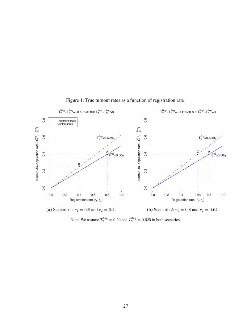
Figure 1: True turnout rates as a function of registration rate

TTReg−TC

Reg=−0.125<0 but TTPop−TC

Pop>0

Registration rate (rT, rC)

Turn

out−

to−p

opul

atio

n ra

te (T

TPop , T

CPop )

Treatment groupControl group

TCPop=0.625rC

TTPop=0.50rT

0.0 0.2 0.4 0.6 0.8 1.0

0.0

0.2

0.4

0.6

0.8

A●

B●

(a) Scenario 1: rT

= 0.8 and rC

= 0.4

TTReg−TC

Reg=−0.125<0 but TTPop−TC

Pop=0

Registration rate (rT, rC)

Turn

out−

to−p

opul

atio

n ra

te (T

TPop , T

CPop )

0.0 0.2 0.4 0.64 0.8 1.0

0.0

0.2

0.4

0.6

0.8

TCPop=0.625rC

TTPop=0.50rT

A●

C●

(b) Scenario 2: rT

= 0.8 and rC

= 0.64

Note: We assume T Reg

T

= 0.50 and T Reg

C

= 0.625 in both scenarios.

27

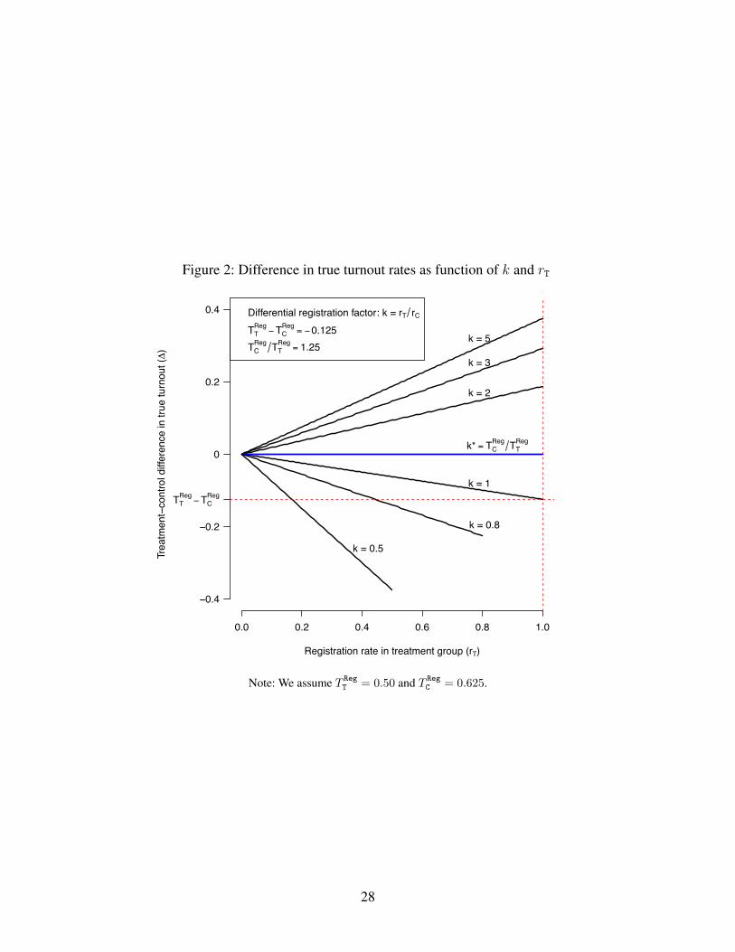
Figure 2: Difference in true turnout rates as function of k and rT

Trea

tmen

t−co

ntro

l diff

eren

ce in

true

turn

out (∆

)

0.0 0.2 0.4 0.6 0.8 1.0

−0.4

−0.2

0

0.2

0.4

TTReg

− TCReg

Registration rate in treatment group (rT)

Differential registration factor: k = rT rC

TTReg

− TCReg

= −0.125TC

Reg TTReg

= 1.25

k = 1

k = 2

k = 3

k = 5

k = 0.8

k = 0.5

k* = TCReg TT

Reg

Note: We assume T Reg

T

= 0.50 and T Reg

C

= 0.625.

28

Figure 3: Total population, registration, and voters for 1986 cohort

0

10000

20000

30000

Treated Control

Total Births

RegisteredVoted

Note: Our data are a random sample from Catalist’s voter file and therefore underestimate the turnout-to-populationrates for both the treatment and control groups. However, because the data were drawn randomly, we can accuratelyestimate the difference in turnout-to-population rates between groups. Voting is measured in the 2008 election;registration is measured in 2011.

29

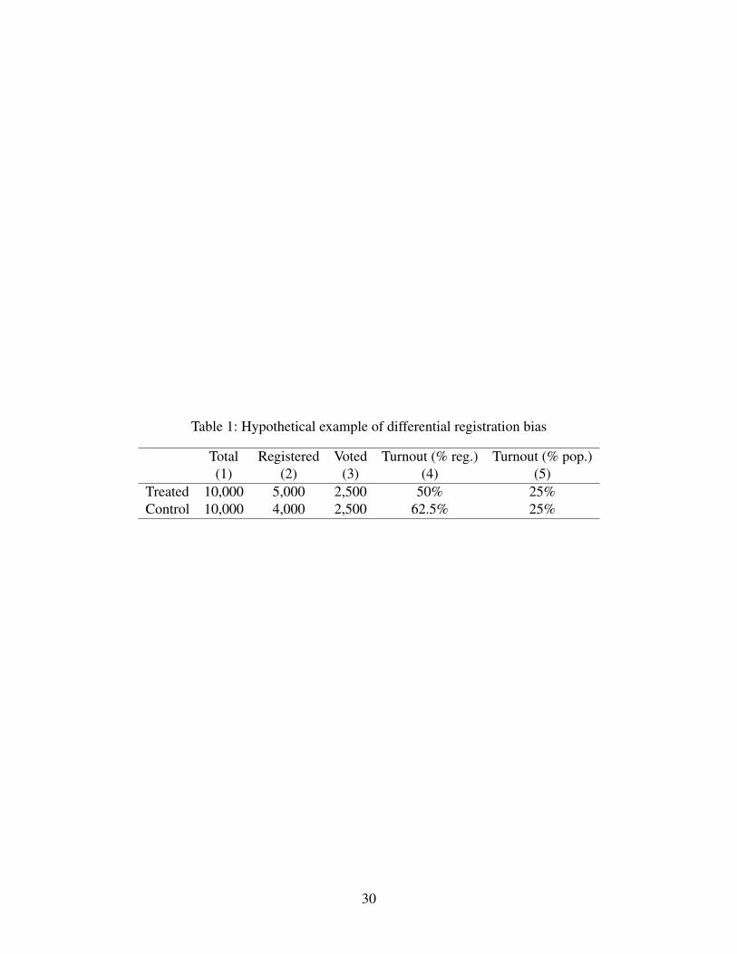
Table 1: Hypothetical example of differential registration bias

Total Registered Voted Turnout (% reg.) Turnout (% pop.)(1) (2) (3) (4) (5)

Treated 10,000 5,000 2,500 50% 25%Control 10,000 4,000 2,500 62.5% 25%

30

Table 2: Hypothetical illustration of sensitivity analysis

Overall populationTotal Registered Voted Turnout (% reg.) Turnout (% pop.)(1) (2) (3) (4) (5)

Treated PT

5,000 2,500 50% 2,500/PT

Control PC

4,000 2,500 62.5% 2,500/PC

31

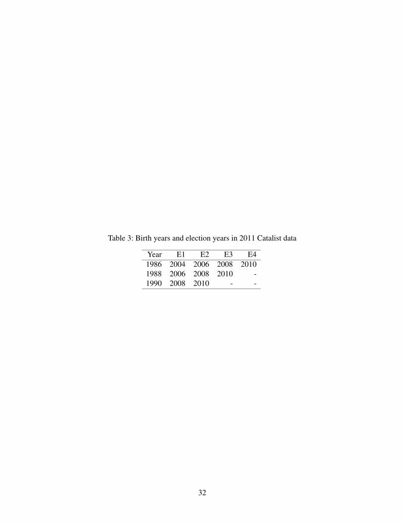
Table 3: Birth years and election years in 2011 Catalist data

Year E1 E2 E3 E41986 2004 2006 2008 20101988 2006 2008 2010 -1990 2008 2010 - -

32

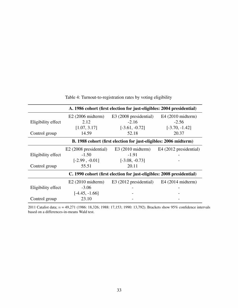
Table 4: Turnout-to-registration rates by voting eligibility

A. 1986 cohort (first election for just-eligibles: 2004 presidential)

E2 (2006 midterm) E3 (2008 presidential) E4 (2010 midterm)Eligibility effect 2.12 -2.16 -2.56

[1.07, 3.17] [-3.61, -0.72] [-3.70, -1.42]Control group 14.59 52.18 20.37

B. 1988 cohort (first election for just-eligibles: 2006 midterm)

E2 (2008 presidential) E3 (2010 midterm) E4 (2012 presidential)Eligibility effect -1.50 -1.91 -

[-2.99 , -0.01] [-3.08, -0.73] -Control group 55.51 20.11

C. 1990 cohort (first election for just-eligibles: 2008 presidential)

E2 (2010 midterm) E3 (2012 presidential) E4 (2014 midterm)Eligibility effect -3.06 - -

[-4.45, -1.66] - -Control group 23.10 - -

2011 Catalist data; n = 49,271 (1986: 18,326; 1988: 17,153; 1990: 13,792). Brackets show 95% confidence intervalsbased on a differences-in-means Wald test.

33

Table 5: Sensitivity analysis


E2 (2006 midterm) E3 (2008 presidential) E4 (2010 midterm)T Reg

T

� T Reg

C

k? T Reg

T

� T Reg

C

k? T Reg

T

� T Reg

C

k?

2.12 0.87 -2.16 1.04 -2.56 1.14


E2 (2008 presidential) E3 (2010 midterm) E4 (2012 presidential)T Reg

T

� T Reg

C

k? T Reg

T

� T Reg

C

k? T Reg

T

� T Reg

C

k?

-1.50 1.03 -1.91 1.10 - -


E2 (2010 midterm) E3 (2012 presidential) E4 (2014 midterm)T Reg

T

� T Reg

C

k? T Reg

T

� T Reg

C

k? T Reg

T

� T Reg

C

k?

-3.06 1.15 - - - -

2011 Catalist data; n = 49,271 (1986: 18,326; 1988: 17,153; 1990: 13,792).

34

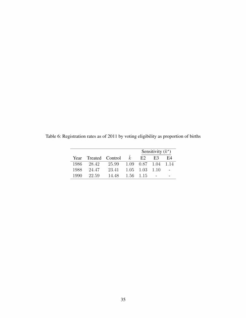
Table 6: Registration rates as of 2011 by voting eligibility as proportion of births

Sensitivity (k?)Year Treated Control k̂ E2 E3 E41986 28.42 25.99 1.09 0.87 1.04 1.141988 24.47 23.41 1.05 1.03 1.10 -1990 22.59 14.48 1.56 1.15 - -

35

Table 7: Turnout rates by voting eligibility as a proportion of births


E2 (2006 midterm) E3 (2008 presidential) E4 (2010 midterm)Eligibility effect 0.96 0.65 -0.23

[0.65, 1.27] [0.13, 1.18] [-0.57, 0.10]Control group 3.79 13.56 5.29


E2 (2008 presidential) E3 (2010 midterm) E4 (2012 presidential)Eligibility effect 0.22 -0.25 -

[-0.28 , 0.72] [-0.56, 0.06] -Control group 12.99 4.71


E2 (2010 midterm) E3 (2012 presidential) E4 (2014 midterm)Eligibility effect 1.18 - -

[0.90, 1.47] - -Control group 3.34 - -

2011 Catalist data; n = 49,271 (1986: 18,326; 1988: 17,153; 1990: 13,792). Brackets show 95% confidence intervalsbased on a differences-in-proportions Wald test.

36

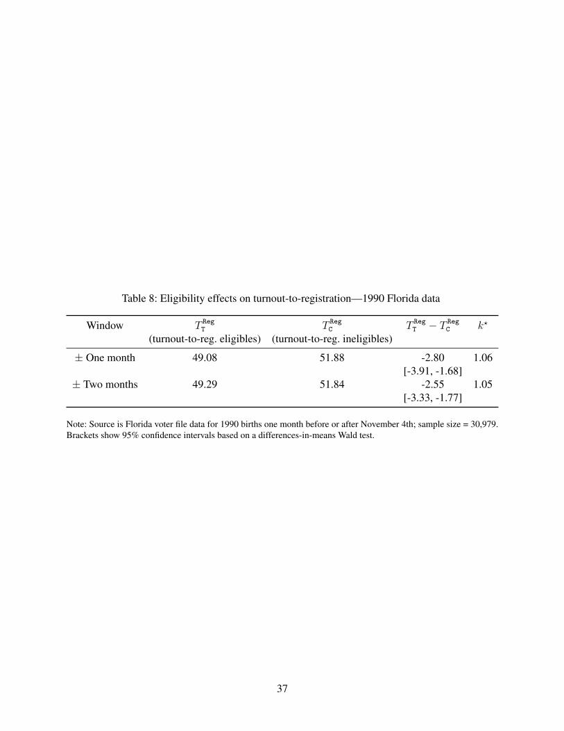
Table 8: Eligibility effects on turnout-to-registration—1990 Florida data

Window T Reg

T

T Reg

C

T Reg

T

� T Reg

C

k?

(turnout-to-reg. eligibles) (turnout-to-reg. ineligibles)

± One month 49.08 51.88 -2.80 1.06[-3.91, -1.68]

± Two months 49.29 51.84 -2.55 1.05[-3.33, -1.77]

Note: Source is Florida voter file data for 1990 births one month before or after November 4th; sample size = 30,979.Brackets show 95% confidence intervals based on a differences-in-means Wald test.

37

Table 9: RD estimates of eligibility effect in 1990 Florida cohort

Denominator T Reg

T

T Reg

C

T Reg

T

� T Reg

C

k̂(turnout eligibles) (turnout ineligibles)

Window of ± one month

Registration 49.08 51.88 -2.80 -[-3.91, -1.68]

Births 44.81 47.48 -2.67 1.11[-3.74, -1.60]

Window of ± two months

Registration 49.29 51.84 -2.55 -[-3.33, -1.77]

Births 48.76 45.41 3.36 1.13[2.61, 4.10]

Note: Florida voter file data for 1990 births within one/two month(s) of November 4th. One-month window samplesize = 30,979. Two-month window sample size = 64,286. Estimated births calculated from Florida vital records forOctober and November 1990. Brackets show 95% confidence intervals based on a differences-in-proportions Waldtest.

38

Supporting Information for “Differential RegistrationBias in Voter File Data: A Sensitivity Analysis

Approach”

Brendan Nyhan⇤ Christopher Skovron† Rocı́o Titiunik‡

Contents

S1 Quality of Catalist data 2

S2 Excluded Catalist data in Study 1 2

S3 Balance checks for Study 1 3

S4 RD plots for Study 1 5

S4.1 Turnout-to-registration rates . . . . . . . . . . . . . . . . . . . . . . . . . . . . . 5S4.2 Turnout-to-births rates . . . . . . . . . . . . . . . . . . . . . . . . . . . . . . . . 7

S5 Results for Study 1 in states without preregistration 9

S6 Birth, registration, and vote totals: Study 1 10

S7 Total births by day and month 10

S8 Sensitivity analysis example: Voting rights restorations 12

⇤Professor, Department of Government, Dartmouth College, [email protected].†Ph.D. Candidate, Department of Political Science, University of Michigan, [email protected].‡James Orin Murfin Associate Professor, Department of Political Science, University of Michigan,

[email protected].

1

S1 Quality of Catalist data

Ansolabehere and Hersh (2010) use Catalist data to analyze the quality of state voter files and find

that “Identifying information such as birthdates are generally well collected.” They do identify

some problems with missing birth dates and unusual concentrations of voters with particular birth

dates but these should not affect the validity of our design.1 Catalist not only cleans and processes

data from state voter files, which includes tracking individuals who move between states and/or

are purged from voter files, but fills in exact birth dates from commercial sources when possible

for states that only release month of birth, allowing us to use exact birthdates even in states that do

not release them.

S2 Excluded Catalist data in Study 1

As mentioned in the paper, we excluded some individuals who were in the raw data provided to us

by Catalist. Table S1 describes the observations excluded by category.

Table S1: Observations excluded from analysis in Study 1

Description Observations

Original dataset 57,031After dropping missing exact birthdates 54,332After dropping outside birth targets 51,705After dropping those recorded as voting when they should have been ineligible 51,472After dropping those with no registration year listed 49,271

1The only unusual date within our window is November 11, which they find to be unusually prevalent in Texas, butwe observe no evidence of a problem in our data (results available upon request).

S3 Balance checks for Study 1

We compare the demographic characteristics of just-eligible and just-ineligible voters for Study 1

in Table S2 using covariates in the Catalist data, which combines public and commercial records

of gender, marital status, race/ethnicity, and religious affiliation. In the pooled data, the differences

in means are small and generally not significant despite the very large sample size.2 As we show

in the paper, though, this seeming balance may mask consequential differences between the two

groups in registration patterns.

2There are a few imbalances in the 1990 cohort, which may be the result of the shorter interval between thetreatment election for this cohort (2008) and the year of data collection (2011).

Table S2: Balance statistics in Catalist data

All Treatment Control p-value

Male 0.464 0.457 0.12Married 0.095 0.095 0.84Black 0.160 0.153 0.04White 0.638 0.645 0.07Hispanic 0.156 0.158 0.52Catholic 0.265 0.272 0.09Protestant 0.275 0.276 0.85

1986 Treatment Control p-value






2011 Catalist data; n = 49,271 (1986: 18,326; 1988: 17,153; 1990: 13,792)

S4 RD plots for Study 1

S4.1 Turnout-to-registration rates

As is conventional in RD analyses, we plot raw turnout rates among registrants binned by date of

birth. Figure S1 illustrates how turnout varies by eligibility in the election after treatment (which

we call E2), while Figure S2 presents corresponding results for the next two elections (E3 and E4).

Figure S1: RD effects of voting eligibility on turnout in subsequent election

●●

●

●●

●

●

●

Eligible in 2004 Ineligible in 2004

10

15

20

25

30

Oct 31 Nov 02 Nov 04 Nov 06Birthdate in 1986

Turn

out r

ate

in 2

006

(a) Turnout effects in 2006 for 1986cohort (E2)

●

●

●

●

●

●

●

●


40

45

50

55

60

65

Nov 05 Nov 07 Nov 09 Nov 11Birthdate in 1988

Turn

out r

ate

in 2

008

(b) Turnout effects in 2008 for 1988cohort (E2)

●●

●

●

● ●

●

●


10

15

20

25

30


Turn

out r

ate

in 2

010

(c) Turnout effects in 2010 for 1990cohort (E2)

2011 Catalist data; n = 49,271 (1986: 18,326; 1988: 17,153; 1990: 13,792). 95% confidence intervals in parentheses.Lines represent means and 95% confidence intervals for just-eligibles and just-ineligibles.

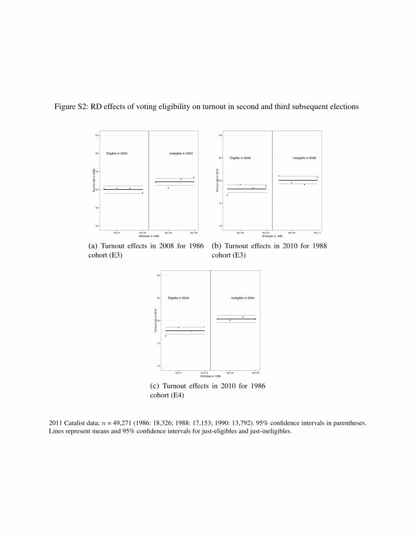
Figure S2: RD effects of voting eligibility on turnout in second and third subsequent elections

● ● ●

●

●

●

●

●


40

45

50

55

60

65


Turn

out r

ate

in 2

008

(a) Turnout effects in 2008 for 1986cohort (E3)

●

●

●

●

●

●

●

●


10

15

20

25

30


Turn

out r

ate

in 2

010

(b) Turnout effects in 2010 for 1988cohort (E3)

●

●

●

●

●●

●

●


10

15

20

25

30


Turn

out r

ate

in 2

010

(c) Turnout effects in 2010 for 1986cohort (E4)

2011 Catalist data; n = 49,271 (1986: 18,326; 1988: 17,153; 1990: 13,792). 95% confidence intervals in parentheses.Lines represent means and 95% confidence intervals for just-eligibles and just-ineligibles.

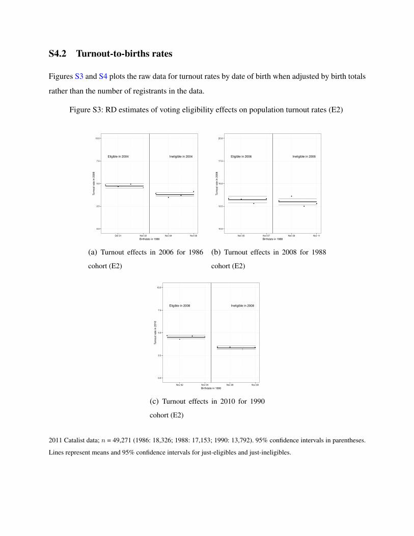
S4.2 Turnout-to-births rates

Figures S3 and S4 plots the raw data for turnout rates by date of birth when adjusted by birth totals

rather than the number of registrants in the data.

Figure S3: RD estimates of voting eligibility effects on population turnout rates (E2)

●●

●

●

●

●

●

●


0.0

2.5

5.0

7.5

10.0


Turn

out r

ate

in 2

006

(a) Turnout effects in 2006 for 1986

cohort (E2)

●●

●

●

●

●

●

●


10.0

12.5

15.0

17.5

20.0


Turn

out r

ate

in 2

008

(b) Turnout effects in 2008 for 1988

cohort (E2)

●

●

●●

● ●

●

●


0.0

2.5

5.0

7.5

10.0


Turn

out r

ate

in 2

010

(c) Turnout effects in 2010 for 1990

cohort (E2)

2011 Catalist data; n = 49,271 (1986: 18,326; 1988: 17,153; 1990: 13,792). 95% confidence intervals in parentheses.

Lines represent means and 95% confidence intervals for just-eligibles and just-ineligibles.

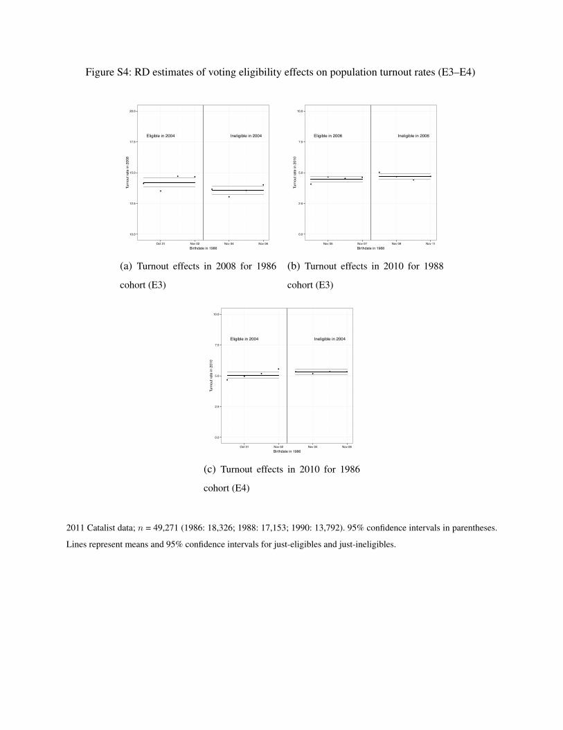
Figure S4: RD estimates of voting eligibility effects on population turnout rates (E3–E4)

●

●

● ●

●

●

●

●


10.0

12.5

15.0

17.5

20.0


Turn

out r

ate

in 2

008

(a) Turnout effects in 2008 for 1986

cohort (E3)

●

●●

●

●

●

●

●


0.0

2.5

5.0

7.5

10.0


Turn

out r

ate

in 2

010

(b) Turnout effects in 2010 for 1988

cohort (E3)

●

●

●

●

●●

● ●


0.0

2.5

5.0

7.5

10.0


Turn

out r

ate

in 2

010

(c) Turnout effects in 2010 for 1986

cohort (E4)

2011 Catalist data; n = 49,271 (1986: 18,326; 1988: 17,153; 1990: 13,792). 95% confidence intervals in parentheses.

Lines represent means and 95% confidence intervals for just-eligibles and just-ineligibles.

S5 Results for Study 1 in states without preregistration

Holbein and Hillygus (2015) argue that preregistration increases mobilization for just-ineligible

voters, who are exposed to the opportunity to preregister. At the time of the elections that we

consider in Study 1, only Florida and Hawaii allowed voters to pre-register when they were 17

years old. Table S3 therefore replicates the main turnout-to-birth analysis of Study 1 (Table 7 in

the main paper) excluding Florida and Hawaii from both the turnout and birth counts. The results

are largely unchanged from the original analysis.

Table S3: Turnout rates by voting eligibility as a proportion of births, excluding preregistrationstates


E2 (2006 midterm) E3 (2008 presidential) E4 (2010 midterm)Eligibility effect 0.89 0.59 -0.28

[0.57, 1.21] [0.06, 1.12] [-0.62, 0.07]Control group 3.79 12.93 5.16


E2 (2008 presidential) E3 (2010 midterm) E4 (2012 presidential)Eligibility effect 0.32 -0.18 -

[-0.18 , 0.83] [-0.50, 0.13] -Control group 12.38 4.54


E2 (2010 midterm) E3 (2012 presidential) E4 (2014 midterm)Eligibility effect 1.20 - -

[0.91, 1.49] - -Control group 3.26 - -

2011 Catalist data; n = 44,167 (1986: 16,385; 1988: 15,371; 1990: 12,411). Brackets show 95% confidence intervalsbased on a differences-in-means Wald test.

S6 Birth, registration, and vote totals: Study 1

This table shows the total number of births, registered voters, and votes cast in the first election

after the eligibility treatment election.

Table S4: Births, registration, and vote totals

1986 treated 1986 control 1988 treated 1988 control 1990 treated 1990 control

Births 31,476 36,096 34,083 37,646 35,537 39,801Registration 8,945 9,381 8,340 8813 8,029 5,763

Votes 1,495 1,369 4,504 4,892 1,609 1,331

Registration and vote totals from 2011 Catalist data; n = 49,271 (1986: 18,326; 1988: 17,153; 1990: 13,792).

S7 Total births by day and month

Figure S5: Total births by month in the United States

●

●

●

●

●

●

● ● ●

●

●

●

2 4 6 8 10 12

2800

0030

0000

3200

0034

0000

3600

0038

0000

Total Births in U.S. in 1986, 1988 and 1990

Month

Tota

l Birt

hs

●

●

●

●

●

●

●

●

●

●

●

●

●

●

●

●

●

●

●

●

●

●

●

●

ooo

198619881990

Source: Vital Statistics of the United States for 1986, 1988 and 1990, Volume I, Natality.

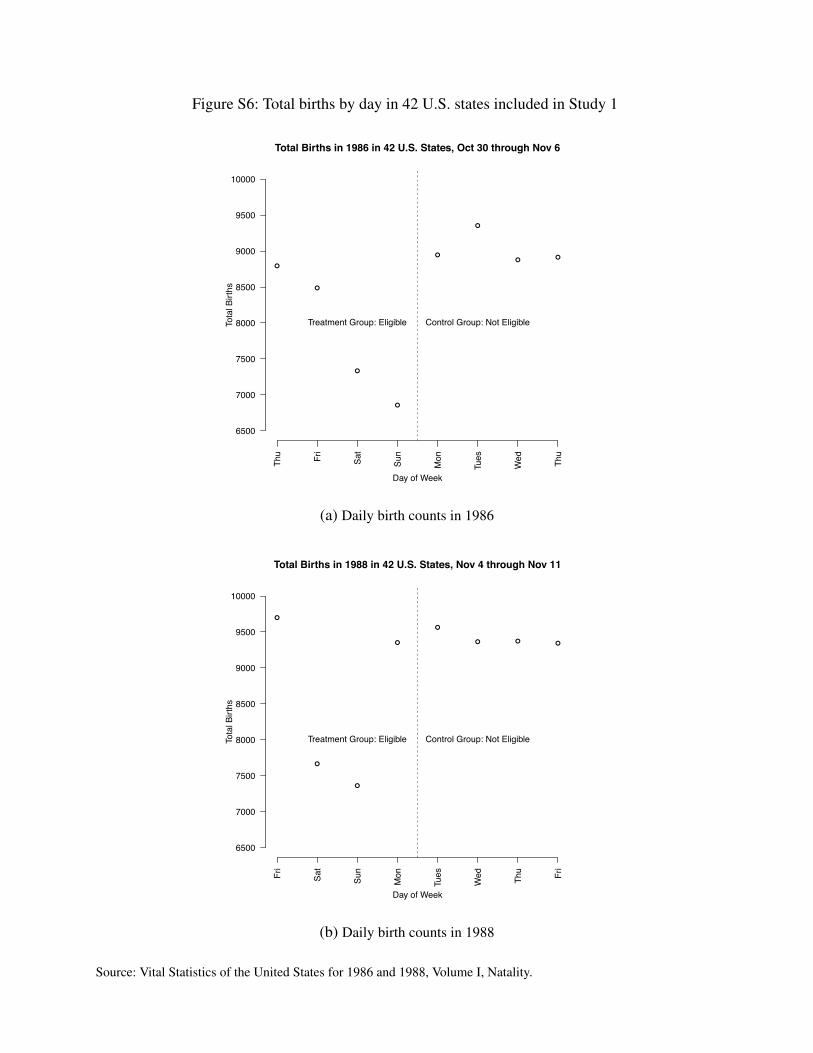
Figure S6: Total births by day in 42 U.S. states included in Study 1

●

●

●

●

●

●

● ●

Total Births in 1986 in 42 U.S. States, Oct 30 through Nov 6

Day of Week

Tota

l Birt

hs

Thu Fri

Sat

Sun

Mon

Tues

Wed Thu

6500

7000

7500

8000

8500

9000

9500

10000

Control Group: Not EligibleTreatment Group: Eligible

(a) Daily birth counts in 1986

●

●

●

●

●

● ● ●

Total Births in 1988 in 42 U.S. States, Nov 4 through Nov 11

Day of Week

Tota

l Birt

hs

Fri

Sat

Sun

Mon

Tues

Wed Thu Fri

6500

7000

7500

8000

8500

9000

9500

10000

Control Group: Not EligibleTreatment Group: Eligible

(b) Daily birth counts in 1988

Source: Vital Statistics of the United States for 1986 and 1988, Volume I, Natality.

S8 Sensitivity analysis example: Voting rights restorations

The problem of differential registration in studies based on voter files is less severe than many

missing data problems because we know that all eligible voters who are not registered did not cast

a vote, leaving only the differential registration factor k to be varied. This approach can be applied

to other research designs in which the size of the treatment and control populations are not known

but outcomes are known with certainty and an intervention could differentially affect the likelihood

of a treatment case being observed compared to a control.

Meredith and Morse (N.d.), for instance, consider differences by race in the rate at which

voting rights restoration applications by ex-felons in Alabama are denied due to outstanding legal

financial obligations (LFOs). In this case, African American ex-felons who are eligible to apply

for restoration of their voting rights are the treatment group, and eligible non-African American

ex-felons are the control group. All outcomes are observed among individuals who petition to have

their voting rights restored—the group that is the equivalent of registered voters in turnout studies.

Moreover, the outcome of interest—voting rights—is known to be 0 among those ex-felons who

do not apply to have those rights restored. However, the size of the treatment and control group

populations are unknown due to limitations on data from the Alabama criminal courts system. The

sensitivity analysis approach we propose can be applied in this case to assess how sensitive these

results are to potential differences in application rates by race.

Another example comes from the literature on international relations. Many analysts study the

likelihood of escalation between states among observed disputes (e.g., Senese 1997). However,

this research design neglects how a treatment of interest might also influence the likelihood of dis-

pute initiation among the unknown set of potential disputes that could be initiated. One potential

approach is to estimate a two-stage selection model (Senese and Vasquez 2003) or a joint model

of the likelihood of onset and escalation (Reed 2000), but scholars who prefer to avoid the strong

distributional assumptions that these approaches typically require could use our sensitivity anal-

ysis approach instead. For instance, Senese (1997) considers the effect of joint democracy (the

treatment of interest) on dispute escalation among the set of qualifying observed disputes between

states. However, joint democracy might affect the likelihood of a dispute being observed among

the universe of potential interstate disputes, producing a form of differential selection bias. Schol-

ars could therefore estimate the sensitivity of an observed difference in escalation rates by dyad

regime type to differential selection among the set of potential disputes.3

References

Ansolabehere, Stephen and Eitan Hersh. 2010. “The Quality of Voter RegistrationRecords: A State-by-State Analysis.” Report, Harvard University. Downloaded August22, 2015 from http://www.eitanhersh.com/uploads/7/9/7/5/7975685/reg_

quality_report_8-5-10.pdf.

Holbein, John B. and D. Sunshine Hillygus. 2015. “Making Young Voters: The Impact of Prereg-istration on Youth Turnout.” American Journal of Political Science Early View.

Meredith, Marc and Michael Morse. N.d. “Discretionary Disenfranchisement: The Case of LegalFinancial Obligations.” Unpublished manuscript.

Reed, William. 2000. “A unified statistical model of conflict onset and escalation.” American

Journal of Political Science 44(1):84–93.

Senese, Paul D. 1997. “Between dispute and war: The effect of joint democracy on interstateconflict escalation.” Journal of Politics 59(1):1–27.

Senese, Paul D. and John A. Vasquez. 2003. “A unified explanation of territorial conflict: Testingthe impact of sampling bias, 1919–1992.” International Studies Quarterly 47(2):275–298.

3An alternate approach that is more common in the literature is to consider selection effects among dyad-yearswhere the treatment and control populations can be fully enumerated.

13

differential registration bias in voter file data: a …nyhan/diff-reg-bias.pdfdifferential...

Documents