difx 2.x rfi mitigation version 0.1.0 gnu gpl 3 this causes ringing in ... 2d projection of figure...

C++ Beamformer Library with RFI Mitigation – Version 0.1.0

DiFX 2.x RFI Mitigation

Version 0.1.0 – GNU GPL 3.0

Max Planck Institute for Radio Astronomy, Jan Wagner

Developed for EU FP7 ALBiUS WP6 D6.3.1 “RFI Mitigation”

Document Version 27. June 2012

1. General This document describes a generic filtering library that was added to DiFX, a popular open source

software correlator conceived by A. Deller [DT03]. DiFX can process several kinds of radio astronomical

observations. Here we concentrate on Very Long Baseline Interferometry (VLBI) and the short-term

antenna array spatial coherence function estimates (visibilities) that DiFX computes.

Radio frequency interference (RFI) is a serious concern for radio astronomy that deals with extremely

faint signals. The most effective method to protect radio science from RFI is legislation and enforcing

radio quiet zones. At increased cost one can also apply signal processing. DiFX provides some RFI

mitigation features. For example, A. Deller 2010 implemented transient signal and RFI detection that

allows bad data to be flagged and discarded.

Following an idea introduced by Roshi and Perley [RP03], the RFI branch of DiFX 2.0.x now provides low-

pass filtering of complex visibilities. In brief, the DiFX correlator outputs time averaged visibility samples.

This process is equivalent to first order low-pass filtering the raw visibility data and resampling the filter

output down to the averaging time. An RFI source not closely tracking the astronomical source will

introduce a high frequency component into unfiltered data. The poor characteristics of the averaging

filter and aliasing allow residual RFI to leak into the correlator output. This causes ringing in VLBI maps.

Steeper low-pass filters replace the time averaging in DiFX and reduce the level of aliased RFI. This

document describes RFI filtering in DiFX. The filter code can be integrated into other correlators, too.

All new C++ and Matlab source code is found in the DiFX repository at https://svn.atnf.csiro.au/difx.

Contents 1. General .................................................................................................................................................. 1

2. Introduction ........................................................................................................................................... 2

3. Additions to Trunk DiFX 2.0.x for RFI Suppression ................................................................................ 6

4. Correlation Job Preparations ................................................................................................................. 7

5. Example vex2difx Input File *.v2d ......................................................................................................... 8

6. Example DiFX Input File *.input............................................................................................................. 9

7. Example Filter Chain File *.coeff ......................................................................................................... 10

8. DiFX C++ and Python Code Additions .................................................................................................. 11

https://svn.atnf.csiro.au/difx


9. Matlab Source Code ............................................................................................................................ 12

10. DiFX Filter Details ................................................................................................................................ 13

10.1. Integrator................................................................................................................................. 14

10.2. Moving average ....................................................................................................................... 14

10.3. IIR Biquad ................................................................................................................................. 15

10.4. Digital State Variable Filter ...................................................................................................... 17

10.5. Decimator ................................................................................................................................ 17

11. Examples on Filtering Behavior ........................................................................................................... 18

12. References ........................................................................................................................................... 26

2. Introduction The “Distributed FX” (DiFX) software correlator created by A. Deller at Swinburne is a popular open

source FX software correlator that runs on computing clusters [DT03]. It is primarily intended for Very

Long Baseline Interferometry (VLBI), a type of interferometry in radio astronomy. While DiFX includes

capabilities for pulsar observations and local phased arrays, this document concentrates on VLBI.

VLBI is synonymous to Earth rotation aperture synthesis interferometry that was first applied to radio

astronomy in the 1950s. Historical and technical details can be found in Interferometry and Synthesis in

Radio Astronomy by Thompson et al. (Wiley, 2nd edition 2001).

DiFX data processing can be divided into roughly two steps, array phasing and array coherence function

estimation. First the astronomical source is delay tracked against Earth rotation and synthetic beam(s)

are steered towards it. Next the array spatial coherence function is estimated over short time intervals

and is output by DiFX. It is used by other software for aperture synthesis and imaging tasks.

For array phasing, each antenna signal is first shifted in time and phase. The shifts are equivalent to

projecting the non-uniform 3D array geometry onto a common plane. Such a projection creates a

coplanar array as shown in Figure 1. The natural choice is a plane that is aligned with the planar wave

front of the astronomical source. As the Earth rotates, the projection needs to be continually adjusted to

keep the array and wave front planes aligned (VLBI “fringe stopping”). The GSFC NASA Calc/Solve

software provides detailed models that correct the basic geometric propagation delay estimates for

atmospheric effects and array geometry deformation due to tidal and tectonic motion.


Figure 1 – Left: Time domain signals from a VLBI antenna array are delay-projected to form a coplanar 2D array, aligned parallel to the astronomical source wave front. Continuous adjustments account for Earth rotation and other effects. The

projection keeps the source stationary at array zenith. Right: Angular response of phased 2D array, six antennas in a uniform linear array with a beam steered towards broadside 0 degrees. Responses for antenna separations (VLBI baseline lengths) of

4, 4.5, 5, 5.5 and 6 wavelengths are overlaid. Any other source like RFI will gradually move through the side lobe pattern.

Next, DiFX phases the coplanar array and steers beams into one or more directions. A simple all-zero

phasing will point a beam towards the stationary source. This is the default beam steering in DiFX.

Additional steerings can be used for multi-beam synthesis i.e. for VLBI “wide field imaging”.

After fringe stopping the astronomical source appears stationary as seen from the coplanar projected

array. As a side effect of the projection, antenna positions in the new array plane gradually drift. This is

essential for the Earth rotation aperture synthesis to sample new portions of the aperture.

Additionally, however, any RFI source will appear to move relative to the source-tracking projection or

fringe stopping function. It is then not stationary relative to the array, but instead experiences an

oscillating phase at different array antennas. Equivalently, for any synthesized single beam the RFI source

would appear to move gradually through the array side lobes, giving rise to time varying interference in

the synthesized beam output data. These effects are shown in Figure 2.


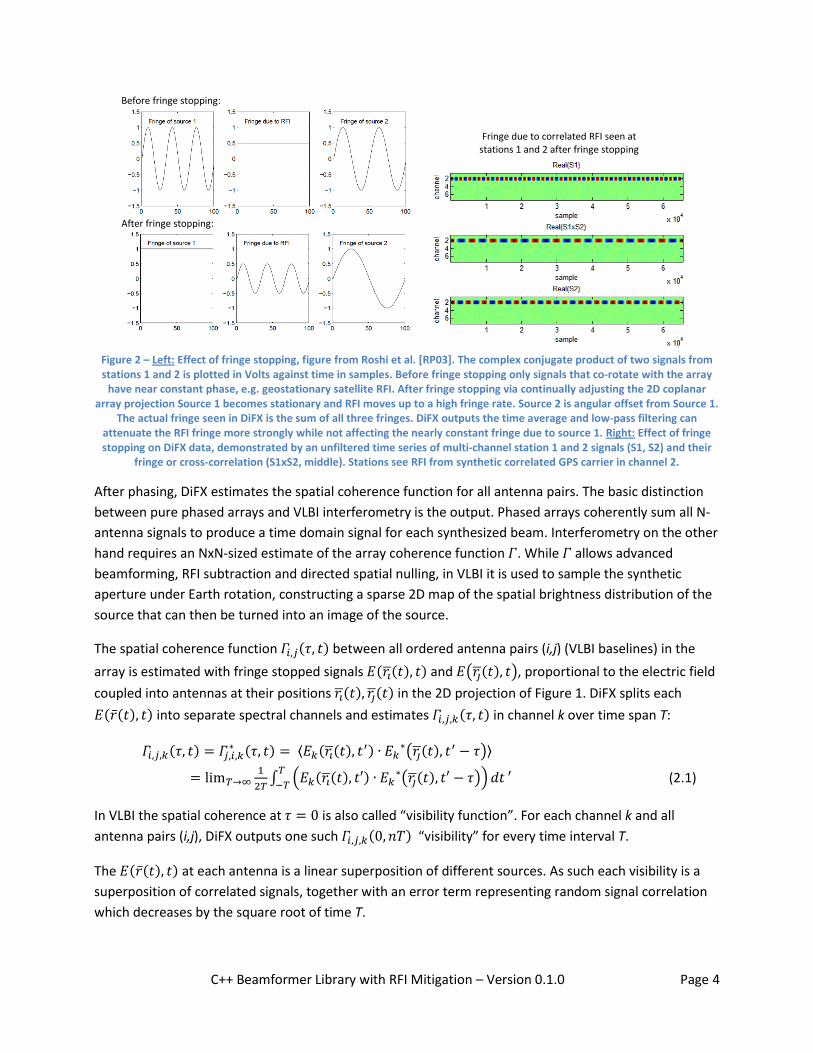
Before fringe stopping:

After fringe stopping:

Fringe due to correlated RFI seen at stations 1 and 2 after fringe stopping

Figure 2 – Left: Effect of fringe stopping, figure from Roshi et al. [RP03]. The complex conjugate product of two signals from stations 1 and 2 is plotted in Volts against time in samples. Before fringe stopping only signals that co-rotate with the array

have near constant phase, e.g. geostationary satellite RFI. After fringe stopping via continually adjusting the 2D coplanar array projection Source 1 becomes stationary and RFI moves up to a high fringe rate. Source 2 is angular offset from Source 1.

The actual fringe seen in DiFX is the sum of all three fringes. DiFX outputs the time average and low-pass filtering can attenuate the RFI fringe more strongly while not affecting the nearly constant fringe due to source 1. Right: Effect of fringe stopping on DiFX data, demonstrated by an unfiltered time series of multi-channel station 1 and 2 signals (S1, S2) and their

fringe or cross-correlation (S1xS2, middle). Stations see RFI from synthetic correlated GPS carrier in channel 2.

After phasing, DiFX estimates the spatial coherence function for all antenna pairs. The basic distinction

between pure phased arrays and VLBI interferometry is the output. Phased arrays coherently sum all N-

antenna signals to produce a time domain signal for each synthesized beam. Interferometry on the other

hand requires an NxN-sized estimate of the array coherence function . While allows advanced

beamforming, RFI subtraction and directed spatial nulling, in VLBI it is used to sample the synthetic

aperture under Earth rotation, constructing a sparse 2D map of the spatial brightness distribution of the

source that can then be turned into an image of the source.

The spatial coherence function between all ordered antenna pairs (i,j) (VLBI baselines) in the

array is estimated with fringe stopped signals and , proportional to the electric field

coupled into antennas at their positions in the 2D projection of Figure 1. DiFX splits each

into separate spectral channels and estimates in channel k over time span T:

(2.1)

In VLBI the spatial coherence at is also called “visibility function”. For each channel k and all

antenna pairs (i,j), DiFX outputs one such “visibility” for every time interval T.

The at each antenna is a linear superposition of different sources. As such each visibility is a

superposition of correlated signals, together with an error term representing random signal correlation

which decreases by the square root of time T.


Correlated RFI with a higher fringe rate tends to integrate towards zero in (2.1) according to the

integrating filter response shown in section 10.1. Correlated RFI typically appears on short VLBI baselines

i.e. close antenna pairs (i,j) that both lie for example in the ground footprint of a satellite transmissions.

Uncorrelated RFI is found mostly in VLBI data at long baselines, where the RFI source is not in common

view of both antennas. Uncorrelated RFI increases the signal power seen by one antenna. This increases

the average of (2.1). This effect can be reduced via the normalized spatial array coherence

(2.2)

in the aperture synthesis and imaging steps. It can be derived from DiFX output data in AIPS or CASA

software post processing, e.g. the old AIPS task ‘ACCOR’.

For correlated and uncorrelated RFI, statistical tests on fringe-stopped VLBI antenna data may

also be used to estimate whether a signal is likely to be RFI.

Some but not all man-made RFI signals are non-Gaussian. Relatively rarely a non-Gaussian signal may

also be a transient of astrophysical origin. In DiFX A. Deller (2010) added higher order statistics for each

VLBI antenna signal. These can be used in a Jarque-Bera test (JB) to reject the null hypothesis that a

signal is Gaussian. The JB test is negative for non-Gaussian data. Non-normality implies data is either RFI-

contaminated and should be discarded in the estimate, or conversely that the data might be of

special interest in an astrophysical transients search.

However, RFI-contamination of data does not imply that the JB test will result in a negative. Many

encoding and modulation schemes produce RFI with sufficiently noise-like flat-top spectra that the JB

test gives a positive result. The detection then fails. Several other RFI or non-normality tests exist, a

comparison can be found in Tarongi et al. [TC10].

The more recent addition to DiFX now is filtering such as in Roshi et al. [RP03]. It can suppress correlated

RFI and improve the coherence estimate by better attenuating any high fringe rate components

such as those shown earlier in Figure 2, that is, RFI sources and other sources at wider angular separation

away from the main astronomical source. The integral in (2.1) is replaced by a filtering function F(s,t):

(2.3)

Using *.coeff filter descriptor files for DiFX one can apply a suitably configured F(s,t) low-pass filter, or a

chain of several low-pass filters. The low pass may also be followed by (2.1) style of time integration.

Combined, this reduces the amplitude of residual correlated RFI that leaks into .

The extensions to DiFX discussed in this document are intended to improve the natural resistance of VLBI

to RFI while not harming the astronomical i.e. low fringe rate sections of the data. Naturally there is a

drawback to filtering. The additional computation in the filters may be expensive and can double the

DiFX processing time. General requirements and a software details as well as results are given below.


3. Additions to Trunk DiFX 2.0.x for RFI Suppression The official SVN source code repository of DiFX is currently found at https://svn.atnf.csiro.au/difx/.

To compile DiFX please see http://cira.ivec.org/dokuwiki/doku.php/difx/installation. You may also join

the developer mailing list at http://groups.google.com/group/difx-users/topics.

Official DiFX 2.0.x (SVN “trunk”) and RFI mitigation branch (SVN tag “rfi”) sources match to an extremely

large degree. The majority of RFI code is separate files and only a few parts of original DiFX needed to be

extended slightly. All changes are listed in Table 1.

The DiFX configuration file has new parameters. At the end of the “COMMON SECTION” in DiFX *.input

files, two new entries are required (‘RFI FILT TYPE’ and ‘RFI FILT COEFFS’). The vex2difx configuration files

*.v2d accept a new option (‘doRFI’). These are described later below.

Table 1 – Code differences compared to trunk DiFX 2.0.x

Program Location in SVN Changes compared to trunk DiFX

mpifxcorr https://svn.atnf.csiro.au/difx/mpifxcorr/branches/rfi/

Syntax additions: INPUT file has new parameters ‘RFI FILT TYPE’, ‘RFI FILT COEFFS’ at the end of the “COMMON SETTINGS” block. Source code integration changes: ~50 lines configuration.cpp/.h: INPUT parsing for both RFI entries core.cpp/.h: calls to filter infrastructure for auto-correlations mode.cpp/.h: calls to filter infrastructure for cross-correlations Source code file additions: ~2700 lines filter*.cpp/.h: new files implementing filter infrastructure

vex2difx https://svn.atnf.csiro.au/difx/applications/vex2difx/branches/rfi/

Syntax additions: ~5 lines V2D file has new optional parameter ‘doRFI’ Source code changes: ~5 lines corrparams.cpp: handles ‘doRFI’ key in V2D file vex2difx.cpp: adds job->rfiFiltertype and job->rfiFilterfile

difxio library

https://svn.atnf.csiro.au/difx/libraries/difxio/branches/rfi/

Source code changes: ~10 lines difx_input.c/.h: reads rfiFiltertype, rfiFilterfile from an INPUT file difx_write_input.c: writes rfiFiltertype , rfiFilterfile to INPUT file

https://svn.atnf.csiro.au/difx/

http://cira.ivec.org/dokuwiki/doku.php/difx/installation

http://groups.google.com/group/difx-users/topics

https://svn.atnf.csiro.au/difx/mpifxcorr/branches/rfi/

https://svn.atnf.csiro.au/difx/mpifxcorr/branches/rfi/

https://svn.atnf.csiro.au/difx/applications/vex2difx/branches/rfi/







4. Correlation Job Preparations The first steps do not differ from normal DiFX 2.0.x preparations. At first, only the usual correlation job

descriptor files need to be prepared. Additional steps required for RFI filtering are bolded.

1. Have VEX file with observation schedule and individual station setups of the VLBI experiment.

2. Have station logs and raw station data recordings from the experiment.

3. Edit VEX file, add station clock offsets (VEX section $CLOCK;) and Earth orientation parameters of

at least 5 days ($EOP;). See http://cira.ivec.org/dokuwiki/doku.php/difx/documentation

4. Use DiFX ‘directory2filelist’ to create per-station lists of raw data files and their time ranges.

5. Create a *.v2d file with the desired correlation setup (VEX file, file lists, correlation channels and

integration time, etc). To enable RFI filtering, add ‘doRFI=True’. An example v2d is in Table 2.

6. Run DiFX ‘vex2difx *.v2d’ to produce several *.input files. These are automatically named, for

example w3oh_1.input, w3oh_2.input, w3oh_3.input, etc, corresponding to each scan. You do

not need to edit these files. An example file is shown in Table 3.

7. Create RFI filter coefficient files *.coeff. One for each *.input file. For example if input files are

named w3oh_*.input , the coeff files would be w3oh_*.coeff. You can copy or symlink a single

file to all the individual scan related *.coeff files. The coeff syntax is shown further below .

8. Run the *.input correlation jobs using the DiFX ‘startdifx’ utility.

Configuration file examples are provided in the next sections.

http://cira.ivec.org/dokuwiki/doku.php/difx/documentation


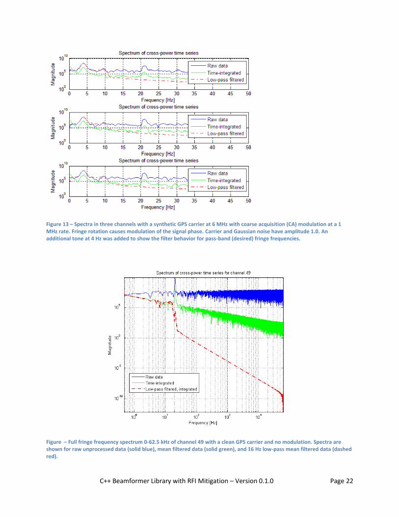
5. Example vex2difx Input File *.v2d An example *.v2d file with the parameter doRFI introduced in RFI DiFX is shown in Table 2.

Low-pass RFI filtering works only on DiFX sub integrations. You can add or update the *.v2d subintNS

parameter and set it closer to the tInt integration time parameter. It must evenly divide tInt.

The limitation comes from DiFX processing the sub integrations in parallel. It adds sub results together in

a random completion order. Correctly filtering the entire tInt across pieces of subintNS would require the

RFI filter state of the previous completed sub integration to be carried over to the next. This implies a

wait and would break the parallelization and decrease performance.

Example: 32 MHz sampling, tInt=2.048s, default subintNS=0.08192s or ≈2.6·106 samples. The tInt is split

into 25 sub integrations. The coeff file low-pass could use f ≥ 1/subintNS = 12.2 Hz to filter out higher

fringe rate RFI. The output tInt is just an average of the 25 subintNS outputs, so very low fringe rate RFI

attenuation does not improve. You may reduce the number of sub integrations by increasing ‘subintNS’.

The cost is higher memory use and a throughput that becomes increasingly I/O constrained.

Table 2 – Example v2d file

Example vex2difx *.v2d descriptor file with RFI-related parameter highlighted # Template v2d file for DiFX correlation of W3OH

vex = w3oh.vex.clocks

antennas = EF, JB, WB

singleScan = True

# The nChan should never be less than 128.

SETUP default

{

tInt = 2.048

nChan = 2048

nFFTChan = 2048

xmacLength = 2048 # to prevent FFT division into 16 x 128-channel pieces

doPolar = True

# enable RFI filters (if unspecified, defaults to False/off)

doRFI = True

# RFI filtering is only applied inside sub-integration time intervals.

# Final summation of the sub-integration outputs does not use a filter.

# To reduce aliasing you may increase the sub-integration time (at cost of RAM).

# Subint of 0.512s will produce 4 subints for the full 2.0s Tint.

subintNS = 512000000 # optional

}

# This, along with SETUP default above, should always be done

RULE default

{

setup = default

}

# Stations and file list locations

ANTENNA EF { filelist = filelist.ef }

ANTENNA JB { filelist = filelist.jb }

ANTENNA WB { filelist = filelist.wb }

# SETUP place holders

SETUP w3oh.set {}

# Sources (pointing centers) with recorded data but no offset pointing centers:

SOURCE W3OH { }


6. Example DiFX Input File *.input The vex2difx tool creates these correlation job descriptor files. You do not need to edit them.

RFI DiFX adds two new fields to the *.input file syntax. They are highlighted in Table 3 below.

Table 3 – Example first lines of an .input file with two new RFI-related entries highlighted in bold.

New fields in RFI DiFX *.input file compared to trunk DiFX # COMMON SETTINGS ##!

CALC FILENAME: /Exps/w3oh/w3oh_01.calc

CORE CONF FILENAME: /Exps/w3oh/w3oh_01.threads

EXECUTE TIME (SEC): 120

START MJD: 55638

START SECONDS: 59651

ACTIVE DATASTREAMS: 3

ACTIVE BASELINES: 3

VIS BUFFER LENGTH: 80

OUTPUT FORMAT: SWIN

OUTPUT FILENAME: /Exps/w3oh/w3oh_01.difx

RFI FILT TYPE: CHAIN

RFI FILT COEFFS: /Exps/w3oh/w3oh_01.coeff

# CONFIGURATIONS ###!

NUM CONFIGURATIONS: 1

CONFIG NAME: W3OH_default

INT TIME (SEC): 2.048000

SUBINT NANOSECONDS: 512000000

…


7. Example Filter Chain File *.coeff A text file specifies the layout and coefficients of the filter chain. It can be “included” from any *.input

file. Auto- and cross-correlations are filtered to assure identical phase and magnitude response in both.

The filter chain can have one or more filters in series. Filter types are: integer factor R decimator, digital

state variable filter (DSVF; has least cost and best low-pass response), integrator (AVG; identical to time

averaging), moving average (MAVG; adjustable window), and arbitrary length IIR filter (IIR-SOS;

implemented as second-order sections, steep but costly).

Table 4 – Example filter chain *.coeff file

Example filter chain coefficients file # ----- Example filter configuration file

# Filter types:

# 0 = Integrator, 1 = Integer Decimator, 2 = IIR biquad, 3 = FIR,

# 4 = Digital State Variable Filter (DSVF), 5 = Moving Average

5 # Number of filters in series, with type and settings in the order below:

# ----- Integrator

0 # type: 0=integrator, has no coefficients

# ----- Integer factor Decimator

1 # type: 1=decimator

3 # decimation ratio

# ----- Biquad IIR Filter

2 # type: 2=IIR-SOS/biquad

10 # filter order, order 10 requires five 2nd order sections

9.99831172521226110e-006 # input prescaling gain

# filter coefficients in M=order/2 rows (M x 6 coeffs total)

# b0(1) b1(1) b2(1) a0(1) a1(1) a2(1)

# ...

# b0(M) b1(M) b2(M) a0(M) a1(M) a2(M)

1.0 -1.99999451637268070 1.0 1.0 -1.99986529350280760 0.99986535310745239

1.0 -1.99999928474426270 1.0 1.0 -1.99989640712738040 0.99989646673202515

1.0 -1.99999964237213130 1.0 1.0 -1.99993586540222170 0.99993598461151123

1.0 -1.99999976158142090 1.0 1.0 -1.99996757507324220 0.99996769428253174

1.0 -1.99999976158142090 1.0 1.0 -1.99999022483825680 0.99999040365219116

# ---- Digital state variable filter

4 # type: 4=DSVF

1.0 # input prescaling gain

0.000773 # tuning f = 2*sin(pi*(1024*(1/0.52))/16e6)

0.5 # quality q = 1/Q=1/2.0

# ---- Moving average filter

5 # type: 5=MAvg

16 # length L of window

0.0625 # input prescaling gain, thus if gain=1/L then output is a moving average


8. DiFX C++ and Python Code Additions The tables below list the new files added to the RFI branch in the DiFX SVN repository. Most of the code

is not tightly integrated and can be tested separately.

Table 5 – Files added to ‘mpifxcorr’ package in DiFX SVN repository

File Description

src/filterchain.cpp,.h Top level filter class that instantiates a chain with one or more filters in series. Allows loading a filter setup from a *.coeff file.

src/filterhelpers.cpp,.h Common utility functions.

src/filter.h Base class for filter functions. All filter types implement the interface.

src/filters.cpp,.h Derived classes and factory function.

src/filter_iirsos.cpp Cascaded bi-quad IIR filter implementation.

src/filter_dsvf.cpp Digital State Variable filter.

src/filter_int.cpp Integrating filter.

src/filter_mavg.cpp Moving average filter.

src/filter_dec.cpp Decimator, sample rate reduction.

tests/filter/ filter_test.cpp Contains a series of tests for the filter infrastructure. Also loads an external 1-channel 32-bit float signal file and filters it with the filter setup from an external *.coeff file.

tests/filter/filter_data.cpp Utility that provides a signal generator (impulse, step, sine, Gaussian noise) and allows the signal to be filtered with an external *.coeff file. The filter output can be plotted in Matlab.

tests/filter/filter_parse.cpp Utility that checks the validity of a *.coeff file.

Table 6 – Files added to other DiFX SVN repository packages

File Description

/utilities/trunk/ datagen5b/datagen5b.py

Generates synthetic Mark5B 16 MHz 8-channel 2-bit recordings for several stations that can be correlated using DiFX. The synthetic data generator provides a GPS signal with carrier, optional C/A and optional Y code modulation. Station recordings share the GPS RFI signal and have uncorrelated additive noise.


9. Matlab Source Code The DiFX SVN repository ‘mpifxcorr’ package contains the relevant Matlab sources under /utilits/matlab/.

Debug dumps can be enabled in the DiFX correlator program ‘mpifxcorr’. A correspondingly named flag

is found in the C++ file ./src/mode.cpp together with a hard-coded output path and file naming

convention. After changes the mpifxcorr program needs to be recompiled.

With dumps enabled, correlation jobs will produce a raw data file for each station. Files contain multi-

channel Fourier transformed complex data after fringe-stopping. It is not filtered or averaged. By default,

all spectral channels are written of only the first sub integration, frequency band and polarization.

The raw data dumps can be loaded into Matlab for inspection, fringe rate analysis and filtering tests.

Table 7 - Matlab source code

Matlab file(s) Function

test_dsvf.m Reference implementation of the Digital State Variable filter for C++.

test_iirsos.m Reference implementation of the bi-quad IIR filter for C++.

fftdump_makefilter.m Returns a filter design (Matlab) used by other fftdump_*.m scripts

read_mk5b.m Helper to read station Mark5B recordings into Matlab.

read_difx_dump.m Reads a chunk of raw (not averaged) multi-channel cross correlation data from a binary file. Dump files are written when DiFX ‘mpifxcorr’ source file ./src/mode.cpp has debug dumping enabled.

load_difx_dump.m Similar to read_difx_dump.m but reads the entire file until EOF.

integrate_difx_dump.m Produces time-integrated autocorrelation from a DiFX dump file.

integrate_difx_dump_xc.m Produces time-integrated cross-correlation from two DiFX dump files.

integrate_difx_dump_xc2.m Produces time-integrated and also filtered cross-correlations from two DiFX dump files.

specgram_difx_dump_xc2.m Reads from two DiFX dump files, produces auto and crosscorrelation spectrograms and a fringe frequency plot. Optional slight pre-averaging.

fftdump_fringerates.m Loads one DiFX dump file and plots the time series of some or all spectral channels, together with a fringe rate plot. When few channels are selected it uses line plots, otherwise a spectrogram plot.

fftdump_fringerates2.m Loads two DiFX dump files. Plots unfiltered, integrated, filtered cross correlation time series. Includes tone insertion at source fringe rate, added noise, filter state initialization variants, other testable options.

fftdump_fringerates2_prexc.m Similar to fftdump_fringerates2.m, but filters station data before forming cross product. The cross product itself is not filtered.

fftdump_checks.m Loads two DiFX dump files. Several plot types can be enabled. Cross correlation spectrogram, time integrated cross- and autocorrelations, phase/lag plot, true cross covariance E<s1*s2’>-E<s1>*E’<s2>.


10. DiFX Filter Details A filter design can be specified in a *.coeff filter chain file. It may contain a mix of different filter types.

DiFX loads filter chain files with the library function FilterChain::buildFromFile(filename, N). This

instantiates an N-channel filter to match the number of spectral channels, half of DiFX FFT/DFT points.

Filtering uses the Intel Performance Primitives (IPP) library that DiFX already links against. All filter

operations are either complex-complex additions or multiplications with real valued coefficients, so the

filter library treats complex input data as real data of twice the length and uses the faster real arithmetic.

The chain filters a discrete time series of samples of one sub integration interval. Input

samples are complex-valued N-channel vectors coming from the DiFX FFT/DFT cross product stage, so

they are the conjugate product of two discrete amplitude samples of antennas a, b in channel i:

(10.1)

The complex conjugate is denoted ‘*’ and discrete time . The antenna data have been fringe-stopped

and Fourier-transformed, so are Fourier domain complex amplitudes in channel i. If antenna

then is a cross-correlation, otherwise it is an auto-correlation.

The sampling rate of is the effective sampling rate in DiFX channels. For example, when station data

sampled at 32 Ms/s is processed with 512 DiFX channels the rate is . Low pass filters will

operate at this channel sampling rate .

Steep low pass filtering with a filter estimates the coherence function . DiFX uses

short sub integration intervals of or samples:

(10.2)

The final DiFX output for a full is always an unfiltered average of all k filtered sub integration results:

(10.3)

Filters can be chained so the output of one filter feeds the next:

(10.4)

Different filters are described below. Some of the attenuation examples use 25.6 Ms/s station data

and 128 channels or = 200ks/s and a sub integration time of 0.5s or a 2 Hz corner frequency . The

low-pass normalized corner frequency is

(10.5)


10.1. Integrator The integrator simply outputs the running sum of all past samples added to it. This filter is identical to

the standard accumulation in the trunk version of DiFX. Filter function and z transform are:

;

(10.1.1)

(10.1.2)

The filter response for a very short length of 4096 samples is shown in Figure 3. Increasing samples

increases the attenuation. The relative attenuation or ratio of gains at and some large is:

(10.1.3)

Figure 3 – Magnitude and phase response of integrator over N=4096 samples. Magnitude normalized to 0 dB. Top panel shows entire normalize frequency range [0, 1(. Bottom panel shows frequency range [0,0.017].

For the top band edge and 200k integrated samples, peak. Near the 2 Hz

integration time attenuation L is less easily evaluated, but with the integrator slope of -20

dB/decade it approaches

.

10.2. Moving average This filter is closely related to the 10.1 integrating filter. It has unity weights for the window length M,

remaining weights are zero. The zero truncation causes pronounced sinc(x)-type ringing at short M.


10.3. IIR Biquad This is an infinite input response (IIR) filter with order 2N. It is

expanded into N cascaded 2nd order IIR filter sections. In this

form the filter is also called bi-quadratic IIR (IIR biquad) or IIR

with cascaded second order sections (IIR SOS).

Coefficients can be generated in Matlab or Octave. A base IIR

filter can be transformed into a SOS Nx6 coefficients matrix

using [sos,g]=tf2sos(b,a). Python SciPy also offers IIR design

functions (scipy.signal.iirdesign) but lacks IIR SOS support.

The IIR SOS has better numerical stability than a plain IIR as it is sufficient to make the individual 2nd

order sections stable. DiFX C++ implements the canonical Direct Form II in Figure 4. Direct Form II has

the least amount of delays, adders and multipliers. This minimizes memory use and arithmetic cost.

The implementation is single precision since DiFX visibilities are single precision data. Note that the

Intel IPP library IIR filter functions are not used since they filter only a single-channel sample

sequences while DiFX visibilities are multi-channel sample sequences.

The response of a single SOS section is:

(10.3.1)

(10.3.2)

Each IIR SOS section has own coefficients , the sixth is fixed to . The DiFX filtering

applies the output of one SOS section to the input of the next, producing the final filtered output:

(10.3.3)

The response for a 8th order four section maximally flat filter with is shown in Figure

5 with a close up of the filter response near the zero normalized frequencies in Figure 6.

Figure 5 – Response of a 8th

order 4-section maximally flat IIR SOS filter with . Normalized frequency range [0, 1(. Magnitude response shown in blue. At double precision (64-bit) the filter reaches 200 dB attenuation quickly.

Figure 4 – Second order section in an IIR SOS DF-II filter. Cascading several such sections

increases filter order.

magnitude response


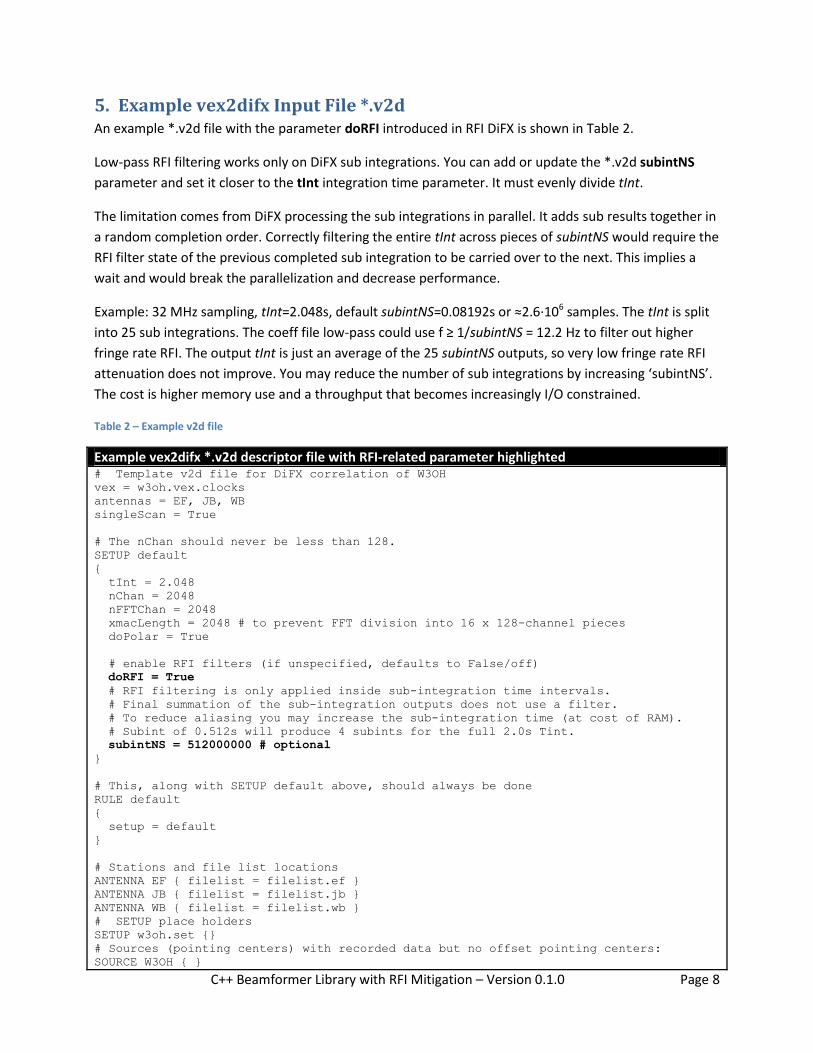
Figure 6 – Same as Figure 5 maximally flat 8th

order filter with with plot showing detail in the low normalized frequency range [0, 1.6e-4]. Filter is double precision.

For single precision arithmetic, one IIR SOS section is stable to about but does not allow a

very strong attenuation. The single precision attenuation can be about 15 dB at . Filter

stability depends strongly on the type of filter design principle (Chebyshev, Butterworth, Elliptic,

Maximally Flat, etc) and it is best to refer to Matlab ‘fdatool’ and the quantizer utility there.

In a DiFX filter chain the IIR SOS filter block can be followed by an integrator to provide further

attenuation, rather than appending the IIR SOS with a decimator and some other filter. This depends

on the desired attenuation.

magnitude response


10.4. Digital State Variable Filter The Digital State Variable Filter (DSVF), also called Chamberlin filter, has the lowest complexity and best

low frequency response of all the above filters. This 2nd order filter was first described in Chamberlin’s

Musical Applications of Microprocessors (1980) and there is a more recent and thorough derivation in

Dattorro [DA97] starting from page 15 (674). The filter structure is shown in Figure 7.

Figure 7 – Chamberlin filter or digital state variable filter. See Dattoro [DA97].

The filter has outputs for high-pass, band reject and low-pass filtered data. The C++ code uses only the

low-pass output. Despite the simplicity of the filter structure in Figure 7, the transfer function H(z) is

quite complex and it is best to refer to the description in Dattorro.

The filter has only two coefficients:

(10.4.1)

(10.4.2)

Coefficient adjusts the tuning and is related to the pass-band center (not cut-off) frequency . This

frequency needs to be less than a fourth the sampling to keep the DSVF stable.

Coefficient is the reciprocal of the quality factor Q. It determines the bandwidth and the damping

factor, or overshoot and settling time. Typically . The filter settles slower but peaks less at the cut

off with and has increasing overshoot with and oscillates at some .

10.5. Decimator The decimator has an adjustable integer decimation factor R. The input rate n is converted to an output

rate m that is a fraction R of the input rate. Aliasing occurs unless x[n] is sufficiently band limited.

; (10.2.1)


11. Examples on Filtering Behavior The effect of low-pass filtering within a DiFX sub integration interval is shown below. A segment of data

from EVN L-band VLBI experiment EW014 on the NGC 1068 extended source was debug dumped to files

by DiFX, before filtering and time integration. A fringe frequency spectrum of one IF and central 32

channels from the Jodrell Bank (JB) - Effelsberg (EF) VLBI baseline data was plotted in Matlab.

Figure 8 – Residual fringe frequency plot from raw, unfiltered 32 channels and 3000 time samples. JB and EF station fringe stopped data was cross-multiplied and then Fourier transformed along the time axis. Left: no additional filtering applied, Right: 2

nd order IIR low-pass filter with a 325 Hz fringe rate cut-off applied. Filtering discards RFI and signals far off from the

main astronomical source which due to fringe stopping has relevant data only at near 0 Hz fringe rate.

The residual fringe rate components (fringes not close to 0 Hertz) are strongly attenuated by introducing

a 2nd order IIR low-pass filter as in Figure 8.

These fringe frequency plots are over a continuous time series of station data. The actual DiFX output

however produces only one visibility for each integration time interval (“final visibility”). A time series

several such final visibilities results is shown in Figure 9 for data from a quasar i.e. point source.


Figure 9 – Series of 46 DiFX output visibilities with a 2.048s integration time and 512 channels. Visibilities are for a quasar i.e. point source seen by the EF-JB baseline. Top: no filtering applied, with a spectrogram of all 46 visibilities on the left, and detail on the 1

st of 46 visibilities on the right, showing magnitude and phase versus channel number as well as the lag

spectrum. Bottom: same 46 visibities with DiFX 2nd

order IIR low-pass filter enabled.

We wrote a Python script (datagen5b.py in the DiFX SVN repository) to generate synthetic data for

several antennas. Antenna signals are derived from a common signal shifted to different time delays with

additive Gaussian noise. The common signal is a sum of a synthetic GPS satellite signal and an

astronomical Gaussian noise source. No Doppler effects and no Earth rotation is applied to the data.

The VLBI model used in DiFX: a GPS satellite and the astronomical source are at the same position at the

celestial north pole. Every station data is basically identical and without time shift but has station-specific

noise added to it. The DiFX correlator uses a fake schedule with the source (phase center) tracking a non-

existent source at +45 degrees declination. The timestamp of the fake Mark5B-format station data was

set to MJD xx556 12:00:00, corresponding to year 2005, month 7, day 5, MJD 53556, DOY 186. Antennas

were EF, WB, MC, TR and the starting elevation is around 80 degrees.


Figure 10 – Modulation of GPS Coarse Acquisition C/A chiplet and P(Y) code onto L1 and L2 carriers. From P. H. Dana http://www.colorado.edu/geography/gcraft/notes/gps/gps_f.html

The GPS satellite signal is synthesized as follows: a sequence S of 1-bit tokens is BPSK-modulated onto

the GPS carrier frequency. According to GPS specifications, sequence S is the product of two codes,

namely the Coarse Acquisition (C/A) 1-bit chip sequence and the Precision P(Y)-code 1-bit data sequence.

The C/A chip sequence is a repetition of 1023 of 0,1 tokens. The 1023-length sequence is a Gold code

and is one out of 37 possible maximally orthogonal and minimally cross-correlated sequences. GPS

assigns one distinct code to each satellite. We use just one satellite. The chip rate is 1.023 MHz, but we

used 1.0 MHz in the data generator.

The P(Y) code is approximated by a uniform random distribution of 0 and 1 tokens. Until the year 1996

the P code was modulated with satellite messages and correction data and it was sent as plaintext. Later,

military level encryption with secret keys was enabled. The encrypted P code is called Y code. We cannot

construct an accurate synthetic Y code sequence because of the encryption. A uniform random sequence

should be an adequate approximation, however. The code rate is 10.23 MHz, we used 10.0 MHz.

Figure 11 – Left: noise-free synthetic GPS C/A (1.023 MHz) without Y code, BPSK-modulated onto 8.0 MHz carrier and sampled at a 32.0 MS/s rate. Power spectrum of 100 milliseconds in linear and log plots and the first 200 signal samples are plotted. Middle: included Y code (10.23 MHz) BPSK-modulation onto 8.0 MHz carrier. Right: unmodulated GPS carrier at 6 MHz with added Gaussian noise floor (σ=1.0,μ=0) with a tone SNR of 2000.

.

http://www.colorado.edu/geography/gcraft/notes/gps/gps_f.html


The pure GPS carrier tone without modulation is placed at 6.0 MHz with peak voltage amplitude 1.0 in

Figure xx. For a 100ms piece of signal data, without 2-bit quantization, the tone has a total signal power

of 0.5 while the Gaussian noise has noise floor with mean 0.4953e-3 and standard deviation 0.2584e-3,

corresponding to an SNR of about 2000.

Synthetic data for four VLBI stations was derived from the GPS data that included the GPS carrier and

common Gaussian noise. First, additional Gaussian noise was added to this data (σ=1.0,μ=0). Without

applying time delays or phase delays this data was then 2-bit quantized using a 1σ magnitude threshold

to get a 16%:34%:34%:16% distribution for the four bit patterns 00:01:10:11. The quantized data was

written into Mark5B data frames. The final output was four Mark5B files, one per station.

Table 8 – Baseline lengths and source start azimuths in synthetic VLBI experiment setup

Baseline to

Station Start Az EF (1) MC (2) TR (3) WB (4)

EF (256) 127deg - 757 km|4.20M 852 km|4.73M 266 km|1.48M

MC (512) 137deg - 1078 km|5.99M 1002 km|5.56M

TR (768) 190deg - 799 km|4.44M

WB (1024) 441deg = 81deg

-

The baselines (if they were oriented exactly East-West) would have a fringe frequency of

f = w_earth * D_lamba * cos(dec) * cos(az) = 7.29115e-5 ; w_earth = 7.29115e-5 rad/sec

EF-MC: f = 7.29115e-5 * 4.20e6 * cos(45*pi/180) * cos(130*pi/180) = -139 Hz

EF-WB: f = 7.29115e-5 *1.48e6 * cos(45*pi/180) * cos(100*pi/180) = -13 Hz

MC-TR: f = 7.29115e-5 * 5.99e6 * cos(45*pi/180) * cos(160*pi/180) = -290 Hz

The DiFX fringe rotation on the EF-MC baselines in the VLBI setup spreads a modulated GPS signal as in

Figure 12.

Figure 12 - Synthetic GPS carrier at 6 MHz with coarse acquisition (CA) modulation at a 1 MHz rate. Carrier and Gaussian noise have amplitude 1.0. Fringe rotation causes modulation of the signal phase.


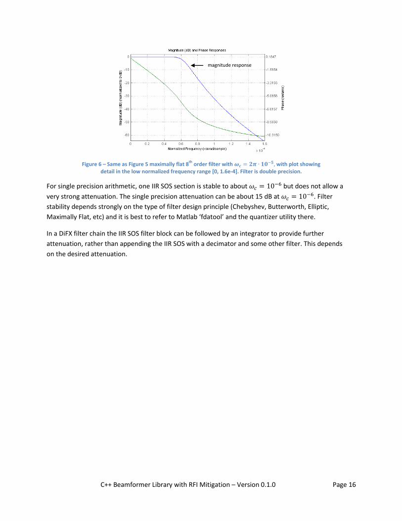
Figure 13 – Spectra in three channels with a synthetic GPS carrier at 6 MHz with coarse acquisition (CA) modulation at a 1 MHz rate. Fringe rotation causes modulation of the signal phase. Carrier and Gaussian noise have amplitude 1.0. An additional tone at 4 Hz was added to show the filter behavior for pass-band (desired) fringe frequencies.

Figure – Full fringe frequency spectrum 0-62.5 kHz of channel 49 with a clean GPS carrier and no modulation. Spectra are shown for raw unprocessed data (solid blue), mean filtered data (solid green), and 16 Hz low-pass mean filtered data (dashed red).


Figure 14 – Unfiltered time series of station 0,1 cross-power for 2 seconds. Stationary GPS tone falls on a fringe rate of 20 Hz.

Figure 15 – Time series as in Figure xx but after time-integrating filter (cumulative sum, normalized). Does not exhibit DC

Figure 16 – Spectra and filter responses. Stationary GPS after fringe stopping at ~20 Hz fringe rate. Gaussian noise was added after fringe stopping to the cross-power to enhance the filter profiles. Settings: 2 seconds of data, XC noise added in Matlab, file channel 49, no pre-fft windowing, filter is 12

th order Chebyshev Type I with 16 Hz cut-off.

Figure 7 – Time series of filter output. Channel 104 contains no GPS signal, no added noise, and only the 2-bit quantization noise (Mark5B input file) of the GPS carrier signal. The 16 Hz low-pass mean filtered data is largely noise free (red). The mean filtered data (green) has residual noise from the 16 Hz to 125 kHz signal range.


Figure 17 – As in Figure 26 except with two-stage filtering applied, low-pass and time integration with normalization.

Figure 18 – Spectrum and time domain output of filtered xcorr: cumulative sum/mean with growing window normalizing only by the current number of samples, versus low-pass followed by cumsum


Figure 19 – Spectrum and time domain output of filtered xcorr: cumulative sum/mean with normalizing by the final number of samples, versus low-pass followed by fixed window cumsum.


12. References [DT03] A.T. Deller, S. J. Tingay et al; DiFX: A Software Correlator for Very Long Baseline Interferometry

Using Multiprocessor Computing Environments, e-print arXiv:astro-ph/0702141, 2003,

http://arxiv.org/abs/astro-ph/0702141

[RP03] D. A. Roshi, R. A. Perley; A New Technique to Improve RFI Suppression in Radio Interferometers,

ASP Conference Series, Vol. 306, 2003; arXiv:astro-ph/0304493v2, 2003,


[TC10] J.M. Tarongi, A. Camps; Normality Analysis for RFI Detection in Microwave Radiometry, Journal of

Remote Sensing, 2010, 2, 191-210, doi:10.3390/rs2010191

http://www.mdpi.com/2072-4292/2/1/191/pdf

[DA97] J. Dattorro; Effect Design: Part 1: Reverbator and Other Filters, AES Journal, Vol. 45, No 9,

September 1997, https://ccrma.stanford.edu/~dattorro/EffectDesignPart1.pdf



http://www.mdpi.com/2072-4292/2/1/191/pdf

https://ccrma.stanford.edu/~dattorro/EffectDesignPart1.pdf

difx 2.x rfi mitigation version 0.1.0 gnu gpl 3 this causes ringing in ... 2d projection of figure...

Documents