DISCUSSION PAPER SERIES

IZA DP No. 11449

Sonja C. KassenboehmerStefanie Schurer

Survey Item-Response Behavior as an Imperfect Proxy for Unobserved Ability: Theory and Application

APRIL 2018

Any opinions expressed in this paper are those of the author(s) and not those of IZA. Research published in this series may include views on policy, but IZA takes no institutional policy positions. The IZA research network is committed to the IZA Guiding Principles of Research Integrity.The IZA Institute of Labor Economics is an independent economic research institute that conducts research in labor economics and offers evidence-based policy advice on labor market issues. Supported by the Deutsche Post Foundation, IZA runs the world’s largest network of economists, whose research aims to provide answers to the global labor market challenges of our time. Our key objective is to build bridges between academic research, policymakers and society.IZA Discussion Papers often represent preliminary work and are circulated to encourage discussion. Citation of such a paper should account for its provisional character. A revised version may be available directly from the author.

Schaumburg-Lippe-Straße 5–953113 Bonn, Germany

Phone: +49-228-3894-0Email: publications@iza.org www.iza.org

IZA – Institute of Labor Economics

DISCUSSION PAPER SERIES

IZA DP No. 11449

Survey Item-Response Behavior as an Imperfect Proxy for Unobserved Ability: Theory and Application

APRIL 2018

Sonja C. KassenboehmerMonash University and IZA

Stefanie SchurerThe University of Sydney and IZA

ABSTRACT

IZA DP No. 11449 APRIL 2018

Survey Item-Response Behavior as an Imperfect Proxy for Unobserved Ability: Theory and Application*

We develop and test an economic model of the cognitive and non-cognitive foundations of

survey item- response behavior. We show that a summary measure of response behaviour –

the survey item-response rate (SIRR) – varies with cognitive and less so with non-cognitive

abilities, has a strong individual fixed component and is predictive of economic outcomes

because of its relationship with ability. We demonstrate the usefulness of SIRR, although an

imperfect proxy for cognitive ability, to reduce omitted-variable biases in estimated wage

returns. We derive both necessary and sufficient conditions under which the use of an

imperfect proxy reduces such biases, providing a general guideline for researchers.

JEL Classification: J24, C18, C83, I20, J30

Keywords: survey item-response behavior, imperfect proxy variables, behavioral proxy, cognitive ability, personality traits, selection on unobservables

Corresponding author:Stefanie SchurerSchool of EconomicsThe University of SydneySydneyAustralia

E-mail: stefanie.schurer@sydney.edu.au

* A previous version of this manuscript was published under the title “Testing the Validity of Item Non-

Response as a Proxy for Cognitive and Non-Cognitive Skills” published as IZA Discussion Paper Nr. 8874 (2015).

The authors acknowledge financial support from an Australian Research Council Early Career Discovery Program

Grant (DE140100463) and the Australian Research Council Centre of Excellence for Children and Families over the

Life Course (project number CE140100027). This paper uses unit record data from the Household, Income and

Labour Dynamics in Australia (HILDA) Survey, which is a project initiated and funded by the Australian Government

Department of Families, Housing, Community Services and Indigenous Affairs (FaHCSIA) and is managed by the

Melbourne Institute of Applied Economic and Social Research. The findings and views reported in this paper, however,

are those of the authors and should not be attributed to either FaHCSIA or the Melbourne Institute. The authors

would like to thank participants of the University of Sydney Microeconometrics and Public Policy Seminar, Monash

University Workshop on Microeconometrics and Panel Data Analysis, and Colin Cameron, Denzil Fiebig, Cheng Hsiao,

David Johnston, Frauke Kreuter, Zhuan Pei, Pravin Trivedi, Peter Siminski, Agne Suziedelyte, Joachim Winter, Mark

Wooden, KennethWolpin, and Jeffrey Wooldridge for helpful comments. Special thanks go to Felix Leung for his

research assistance during the early stages of the manuscript.

1 Introduction

Survey methodologists have recognized that survey item-response is closely related to respon-

dents’ individual attributes (Beatty and Herrmann, 2002; Dillman et al., 2002). Previous studies

have highlighted cognitive abilities (e.g. Tourangeau, 2003) and personality traits (Weijters et al.,

2010; Wetzel et al., 2016) as key attributes that shape response patterns.1 The cognitive model of

survey item-response behavior concedes that individuals consider question complexity and rel-

ative costs before responding to survey questions (Sudman et al., 1996; Schwarz and Oyserman,

2001). Better cognition, diligence, andwillingness to cooperate are likely to reduce the (perceived)

cost of responding to even highly complex questions, which in turn increases the probability of

response

Economists acknowledge cognitive and non-cognitive abilities2 as two distinct components

of adult human capital that can be fostered through education, but that are hard to measure

(Schurer, 2017; Kautz et al., 2014; Heckman and Kautz, 2014; Almlund et al., 2011). In this studywe

ask whether individuals’ survey response behavior may provide insights into their abilities. We

suggest that the survey item response rate (SIRR) – which is calculated as the fraction of survey

items responded to by each individual – could be a convenient proxy for often unobserved or

poorly-measured cognitive and non-cognitive ability. Its appeal lies in its simplicity; variation in

item response rates are a side-product of every survey. SIRR could prove useful when included as

an additional control variable in data applications that are plagued by unobserved confounders.

Previous studies have exploited such paradata – data captured during the process of producing

a survey statistic (Kreuter, 2013) – to fix estimation biases due to selection or heaping behavior

(Pudney, 2014; Heffetz and Rabin, 2013; Kleinjans and van Soest, 2014; Behaghel et al., 2015).

However, there is little empirical evidence on the link between SIRR and standard measures of

cognitive and non-cognitive abilities, nor on the potential of SIRR to address ability-related esti-

mation biases.3

1Other factors that have been suggested are the survey mode, interviewer characteristics, question topic andstructure, question difficulty, institutional policies (Dillman et al., 2002).

2In this study we use the term non-cognitive abilities interchangeably for personality traits; other terms com-monly used in the literature are character traits, soft skills, life skills, or non-cognitive skills.

3The economics literature covered in depth survey measurement error, recall bias and unit non-response, but haspaid little attention to item non-response with the exception of e.g. Riphahn and Serfling (2005) and Raessler andRiphahn (2006). Most of the research in this area investigates the determinants of non-response to sensitive questions

1

To guide our empirical investigation, we first develop an economic model of the cognitive and

non-cognitive foundations of survey item-response behavior. This theoretical model stipulates

that cognitive and non-cognitive abilities affect both themarginal costs and benefits of responding

to a survey question, and thus influence the optimal number of survey questions responded to in

equilibrium. For instance, higher levels of cognitive ability increase the opportunity cost of each

question, reducing the number of questions responded to. Yet, they also decrease the perceived

psychic cost of responding by reducing the time needed to answer each question, thus increasing

the number of questions responded to. The model predicts that if the decrease in psychic cost

outweighs the increase in opportunity cost, we will observe a positive relationship between cog-

nitive ability and survey-item response. Similar predictions are derived for non-cognitive ability.

We test the predictions of the model using nationally-representative survey data from Aus-

tralia. The advantage of these data is that skills and survey response behaviors were measured

by two separate components of the survey; an interviewer-assisted questionnaire with high and

non-variable item-response rates, and a self-completion questionnaire characterized by lower and

more variable item-response rates. We demonstrate a strong relationship between SIRR calcu-

lated from the self-completion questionnaire and standard task-based, interviewer-administered

measures of cognitive ability, ceteris paribus. From a statistical perspective, SIRR behaves simi-

larly to cognitive ability: it has a strong individual-fixed component, and is predictive of economic

outcomes. This interpretation provides evidence in support of the model, suggesting that the re-

duced psychic costs produced by higher cognitive ability outweigh the increased opportunity

costs. In contrast, SIRR is only weakly associated with non-cognitive skills, suggesting that the

combined benefits and reduced psychic costs resulting from an individual’s personality traits do

not outweigh the increased opportunity costs.

Building on our empirical findings, we argue that SIRR – although likely to be imperfect –

(wages, income, wealth) or adjusts the estimates of the determinants of wages, income or wealth equations to it(Zweimueller, 1992; Riphahn and Serfling, 2005; Bollinger and Hirsch, 2013; Bollinger and David, 2005). Some recentexceptions are Hedengren and Stratmann (2013) and Hitt and Trivitt (2013) who tested explicitly the hypothesisthat personality traits are associated with item non-response using US and German longitudinal data. Both studiesshow evidence of a significant association between conscientiousness, a key component of the Big-Five personalitytraits, and item non-response. Zamarro et al. (2016) use data from the Understanding America Study, a nationallyrepresentative internet panel, to study the validity of innovative measures of character skills based on measures ofsurvey effort. A recent study by Hitt et al. (2016) demonstrates that survey effort of youth is highly predictive oflater-life educational attainment, using data from six nationally representative data sets. The authors judge thatsurvey effort is a behavioral measure for conscientiousness.

2

could be used as a proxy variable for cognitive ability to reduce omitted-variable biases (OVB).

To do so, we first present a conceptual framework and derive the necessary and sufficient con-

ditions under which imperfect proxy variables reduce OVB. We illustrate how these conditions

can be used as a guideline by researchers for evaluating the risks of employing an imperfect

proxy variable approach, a tool of general applicability. This conceptual framework is then ap-

plied to a standard wage regression model, the most widely used application by economists to

illustrate methodological points,4 to quantify the bias-reduction potential of SIRR as a proxy for

unobserved cognitive ability. Because we observe both the proxy and cognitive ability, we can

calculate the exact bias reductions in the returns to education and locus of control, a widely stud-

ied non-cognitive skill (see Cobb-Clark, 2015). We demonstrate that SIRR is indeed an imperfect

proxy, but it reduces OVB in the wage returns to education and locus of control by roughly 10%.

Item-response behaviors for the most cognitively demanding questions, such as those on com-

puter use, time diaries, and household expenditures, are most powerful for bias reduction.

Our study contributes to the human capital and statistical literature in three important ways.

First, we complement recent work on identifying task-based or observational measures of abil-

ity. This emerging literature raises the question of whether standard instruments used to mea-

sure cognitive or non-cognitive ability yield what researchers intend to capture (see Lundberg

(forthcoming), Borghans et al. (2016), and Almlund et al. (2011) for a discussion of these issues).

Behavioral measures have been used in the literature to circumvent measurement problems or

unavailability of standard instruments. Many studies use administrative records on student be-

havior to proxy non-cognitive abilities including school attendance rates, number of suspensions

(Jackson, 2017; Dee and West, 2011; Holmlund and Silva, 2014; West et al., 2016), participation

in extracurricular activities (Lleras, 2008), or behavior in class (Heckman et al., 2013). To proxy4Wage regression models are the textbook example to illustrate OVB (see Angrist and Pischke, 2009, on the

returns to education). For recent applications, see Pei et al. (2018) and Oster (2017). In the context of the Theory ofHuman Capital, unobserved cognitive ability is one of the most-often cited factors that cause OVB. The discussion onthe confounding role of unobserved ability emerged in the early 1960s when economists debated whether educationboosts skills and productivity or whether self-selection into education by ability is the reason for the high returns toeducation found empirically (see Gronau, 2010, for a review). Concerns over OVB due to unobserved ability are stilldominating the empirical literature, giving rise to ever-more innovative methods – that entail their own limitations– to identify a causal effect of education on earnings (e.g. Blackburn and Neumark, 1993; Ashenfelter and Rouse,1998; Card, 2001; Oreopoulos, 2006; Heckman et al., 2017), health outcomes (Chatterji, 2014; Heckman et al., 2017)and health behaviors such as smoking (Heckman et al., 2017). A similar discussion has emerged in the literature thatestimates the causal impact of non-cognitive skills on economic outcomes (see Almlund et al., 2011, for an overview).

3

conscientiousness, Hitt et al. (2016) use information on survey effort, while Heine et al. (2008) use

information on walking speed and the accuracy of clocks. Kautz et al. (2014) suggest that "perfor-

mance on any task or any observed behavior can be used to measure personality and other skills"

(p. 16), and conclude that as long as such a measure predicts behavior and can be implemented in

practice, it is useful. With the exception of Hitt et al. (2016) and West et al. (2016), none of these

studies have validated their behavioral proxies.

We also contribute to the dormant and predominantly theoretical literature on proxy variable

biases (Wickens, 1972; McCallum, 1972; Aigner, 1974; Frost, 1979). We extend this theoretical

literature by showing that a strong proxy is neither a necessary nor a sufficient condition for

reducing OVB. The necessary condition requires sign equivalence of two key correlation coeffi-

cients: the partial correlation between the missing variable and the proxy (strength of the proxy),

and the partial correlation between the missing variable and the variable of interest (degree of

OVB). The sufficient condition bounds the ratio of the strength of the proxy to the degree of OVB

– a term we refer to as the relative strength of the proxy – by terms that only depend on the

degree of multicollinearity introduced into the model by the proxy, which is always observable.

There has been a paucity in empirical research testing the validity of proxy variables even

though proxies are widely used in microeconomic applications. Yet, testing is important, because

an imperfect proxy variable – that is, a proxy that correlates with the key variable from the

regressionmodel – may exacerbate biases (see Frost, 1979;Wolpin, 1995, for a formal discussion).5

Practical guidelines for such testing are non-existent. Todd and Wolpin (2003) rightly suggested

that "in some sense, the problem of whether or not to include proxy variables is insoluble, because

it involves a comparison between two unknown biases" (p. F15). Nevertheless, we offer a solution

to this theoretical dilemma – a practical guideline which can be used to evaluate the potential

estimation biases resulting from an imperfect proxy.

Third, we contribute to a broader literature on causal inference in the presence of unobserved

confounders (Rosenbaum and Rubin, 1983). Recent work by Oster (2017) and Altonji et al. (2005)5Apart from task-based behavioral proxies which we consider in this study and that have been used in previous

research as discussed above, proxies are also widely used as inputs in the educational production function, suchas family income to compensate for family investments into children (Todd and Wolpin, 2003). Proxies have alsobeen used to measure unobserved wage offer distributions in a hazard model of unemployment durations, a choicecriticized by Wolpin (1995) who showed in detail the implications of an imperfect, or what he refers to as a ‘crude’proxy variable in the context of a job-search model.

4

provide bounds on estimation biases that depend on assumptions about the maximal possible

degree of explained variation in the outcome of interest and the relative importance of unob-

servable over observable selection into treatment.6 Our approach requires different and arguably

less restrictive assumptions if information on the nature of the unobserved confounder is avail-

able. Comparing the bias-reduction potential of the proxy variable approach against the methods

proposed in Oster (2017), we conclude that in certain situations the proxy variable approach is a

good alternative.

Our work is closely related to Pei et al. (2018), who demonstrate that in the presence of poorly

measured confounders, an alternative empirical tool kit should be used than the “coefficient-

comparison test” to test the identification assumption of a regression strategy. Although our ap-

proach is also centered on the problem of poorly measured right-hand-side control variables, we

focus on a different implication regarding this concern. Pei et al. (2018) highlight that a sensitivity

check with poorly-measured additional control variables may lead to the erroneous conclusion

that the identification assumptions of the model hold, misleading researchers into believing that

OVB play no role. We emphasize, in contrast, that adding a poorly measured right-hand-side

variable may exacerbate OVB.

The remainder of this paper is structured as follows. In Section 2 we lay out an economic

model on the cognitive and non-cognitive foundations of item-response behavior. In Section 3 we

describe the Household, Income, and Labor Dynamics in Australia (HILDA) survey which we use

for testing the predictions of our economic model. In Section 4 we derive necessary and sufficient

conditions of a valid but imperfect proxy variable, and translate these into an empirical guideline.

Section 5 presents test results of using SIRR as a proxy for cognitive ability in the context of wage

returns to education and locus of control. Section 6 concludes. An Online Appendix provides

supplementary material.6This literature extends previous approaches that explicitly model unobservable selection into treatment (e.g.

Murphy and Topel, 1990; Imbens, 2003) or which vary the set of control variables as sensitivity analyses (Heckmanand Hotz, 1989; Dehejia and Wahba, 1999; Gelbach, 2016).

5

2 An economic model of survey item-response behavior

Why is survey item-response behavior related to cognitive ability and personality traits? The

following, brief theoretical framework highlights the relevant behavioral channels and motivate

our empirical analysis. We base our theoretical model on Dillman (2000)’s theory on survey par-

ticipation. This model originates from social exchange theory developed by Homans (1961) and

Blau (1964). It assumes that people engage in social interactions because they receive something

in return. Individual i replies to question j (Rij = 1) if the expected benefits Bij outweigh the

expected costs Cij. E[.] indicates expectations:

Rij = 1 if E[Bij(Pi, FIi) − Cij(Oij, Sij)] > 0, (1)

= 0 otherwise.

The expected benefits are a function of personality trait Pi and a financial incentive FIi if paid

to complete the survey as a compensation for lost time. Individuals are more likely to respond to

the question, if they are paid a dollar amount for each response. We therefore assume that ∂Bij

∂FIij>

0, independent of the individual’s personality or cognitive ability.7 Furthermore, personality may

affect survey response because some individuals want to contribute to a public good (e.g. they

are agreeable or conscientious), or because they derive pleasure from talking about themselves

(see Singer and Ye, 2013). We assume that the marginal benefits due to personality trait P are

MBP =∂Bij

∂Pi> 0.

Survey item response on each question j comes at a cost to the individual. Expected costs

E(Cij) include both opportunity costs Oij and psychic costs Sij:

E(Cij) = E(Oij(Wi(Ai, Pi)) + Sij(T(Ai, Pi))). (2)

We assume that the highest-valued opportunity foregone due to the time spent completing

the survey is working, which can be quantified by wages Wi. Wages depend on both cognitive7In our empirical example there are no financial incentives paid for completing the self-completion questionnaire,

and thus we abstract from financial incentives as determinants of survey item-respose. As an extension to this model,one could argue that the marginal response to financial incentives differs by cognitive ability or personality.

6

ability Ai and personality trait Pi.8 Therefore, we assume that the marginal opportunity costs

due to cognitive ability are MC|AO =∂Oij

∂Wi

∂Wi

∂Ai> 0 and due to personality traits are MC|PO =

∂Oij

∂Wi

∂Wi

∂Pi> 0.9

Answering survey questions is also mentally demanding and therefore places psychic costs

on individuals for the time Tij they have to endure the full survey. These psychic costs depend on

the (perceived) time it takes to answer each question. The total time needed to respond is shorter

for individuals with higher levels of cognitive abilityA and personality trait P. Time to answer is

reduced by cognitive ability because an individual has to understand the meaning of the question,

recall relevant behavior and information, infer the appropriate answer and map the answer into

the response format of the survey (Schwarz and Oyserman, 2001). The higher cognitive ability

A is, the lower the mental demands associated with answering a given question. We therefore

assume that the marginal psychic costs due to cognitive ability are MC|AS =∂Sij

∂Tij

∂Tij

∂Ai< 0.

Furthermore, replying to a question may entail revealing information about personal life and

carefully and diligently reading and replying to each question (Singer and Presser, 2007). There-

fore, the psychic costs will be lower for individuals with certain personality traits, such as open-

ness to experience, extraversion and conscientiousness, because the respondent derives less disu-

tility from every minute spent on answering the question. Such attributes allow individuals to

more easily engage with an interviewer, overcome privacy and confidentiality concerns, and pa-

tiently and diligently go through a questionnaire. We therefore assume that the marginal psychic

costs due to personality trait P are MC|PS =∂Sij

∂Tij

∂Tij

∂Pi< 0.

The model highlights that the decision to reply to a specific question depends on the trade-

offs between perceived costs and benefits, and the trade-offs between taking less time to respond

but facing greater opportunity costs for time spent on the survey. In the optimum, the individual

will respond to the question when the marginal benefits due to increases in Ability Ai are equal

to or greater than the marginal costs due to increases in Ability Ai:8Alternatively, one could assume that opportunity costs could refer to time lost for studying or time spent with

children. We will acknowledge this possibility in our empirical specification.9There is sufficient evidence in the literature that wages depend on both cognitive and non-cognitive abilities.

See Almlund et al. (2011) for a review of the literature and Elkins et al. (2017) for more recent evidence.

7

MBA > MC|AO −MC|AS . (3)

Since MBA = 0, it must follow that MC|AS > MC|AO. Thus, as long as the marginal psychic

cost reductions due to cognitive ability are at least as large as the increases in marginal opportu-

nity costs, then the individual will respond to question j.

In the optimum, the individual will also respond to the question if the marginal benefits are

equal to or greater than the marginal costs due to changes in personality trait Pi:10

MBP > MC|PO −MC|PS, (4)

MBP +MC|PS > MC|PO. (5)

SinceMBP > 0,MC|PO > 0 andMC|PS < 0 this condition implies that the individual decides

to respond to question j if the combined increases in marginal benefits and reductions in psychic

costs outweigh the increases in marginal opportunity costs due to personality trait Pi.

In the next two subsections we illustrate implications of the economic model’s derivations for

the aggregate level, leading to empirically testable predictions.

2.1 Model predictions for cognitive ability

Figure 1 summarizes graphically what happens in the aggregate – over the full duration of the

survey – for individuals of different cognitive and non-cognitive abilities. The horizontal axis

describes the number of survey questions responded to, where Qmax is the maximum number

of survey questions (complete survey), and Qmin the minimum number of questions necessary

to be counted as survey participant. The vertical axis describes the implicit "price" which needs10Note, we are assuming additive separability in the inputs personality trait P and cognitive ability A. This may

be a strong assumption, yet we argue that the predictions of the model will be the same, but stronger, if we allowedfor interaction effects between personality and cognitive ability. Since the marginal cost responses of personalityand cognitive ability are moving into the same direction, we will be facing the same tradeoffs when exploring thecase of higher or lower levels of both personality trait P and cognitive ability. The only difference will be if allowingfor high levels of cognitive ability and low levels of personality trait P, or vice versa. We leave this special case forfuture research.

8

to be paid to the participant for responding to every additional question. The marginal cost (MC)

curve is upward sloping, and the marginal benefit (MB) curve is downward sloping, assuming

that the benefit for every additional question declines and the cost for every additional survey

question increases. Where marginal cost and benefit curves intersect indicates the total number

of survey questions responded to by the participant (Q∗1).

Figure 1(a) shows that cognitive ability affects only the slope of the marginal cost curve. On

the one hand, because of its negative impact on psychic costs, it makes the marginal cost curve

flatter – a move from MC1 to MC2 – and thus the optimal number of questions answered is

larger (Q∗2). On the other hand, because of its positive impact on opportunity costs, it makes

the marginal cost curve steeper – a move from MC1 to MC3 – and thus the optimal number of

survey questions answered is smaller (Q∗3).

This model allows for three different predictions. Cognitive ability may be positively, nega-

tively, or not at all associated with survey item response, depending on the dominance of the

psychic cost response over the opportunity cost response. Empirically, we can test for this re-

lationship by estimating a reduced-form OLS model, in which SIRR is regressed on a measure

of cognitive ability and other controls. A positive relationship is evidence that psychic cost re-

sponses outweigh opportunity cost responses of cognitive ability (MC2); a negative relationship

is evidence for the reverse (MC3); and no association is evidence that psychic cost responses

neutralise opportunity cost responses.

2.2 Model predictions for personality

Figure 1(b) shows that personality affects the slope of both the marginal cost and the marginal

benefit curves. Similar to cognitive ability, personality trait P steepens the marginal cost curve –

a move fromMC1 toMC3 – but also flattens the psychic cost curve, a move fromMC1 toMC2.

Personality trait P also flattens the marginal benefit curve – a move fromMB1 toMB2 – so that

for every additional survey question, the associated reduction in marginal benefits declines. For

instance, a survey participant with high levels of personality trait P ends up responding to all

possible questions (Qmax), under the assumption that psychic costs outweigh opportunity costs.

Again, the model allows for three predictions. Personality may be positively, negatively, or

not at all associated with survey item response, depending on the dominance of the opportunity

9

cost response over the combined psychic cost and benefit responses. Empirically, we can test

for this relationship by estimating a reduced-form OLS model, in which SIRR is regressed on

a measure of personality and other controls. A positive relationship is evidence that combined

psychic cost and benefit responses outweigh opportunity cost responses of personality (MC2);

a negative relationship is evidence for the reverse (MC3); and no association is evidence that

combined psychic cost and benefit responses neutralise opportunity cost responses.

In the following section we test the economic model of survey item-response behavior before

we consider using SIRR as a proxy variable for unobservable confounding ability variables in

wage regressions.

3 Testing the economic model of survey item-response behavior

In this section we outline the data we use in the analysis before testing the predictions of the

theoretical model and provide further evidence on whether SIRR behaves in a statistically similar

way to abilities.

3.1 Data: Household, Income and Labour Dynamics in Australia Survey

We use data from the HILDA survey which is a nationally representative household panel study

conducted annually since 2001 (Summerfield, 2010). The survey comprises a household question-

naire, a person questionnaire for each household member, and a self-completion questionnaire.

All adult household members aged 15 years and above are invited to respond to an interviewer-

assisted (continuing or new-person) questionnaire, in which information on education, employ-

ment, or family formation is collected. In addition, each eligible household member is invited

to complete a self-completion questionnaire (SCQ) to be filled out in private. This SCQ collects

predominantly attitudinal questions. The interviewer collects the completed SCQs at a later date

or, if a date cannot be arranged, the household is asked to return the SCQ by mail. Some house-

hold members opt to return a completed SCQ before the interviewer conducts the face-to-face

interview.11

11The household form takes about 10minutes to complete while each person questionnaire takes about 35minutes.The SCQ takes also about 30 minutes to complete. HILDA pays a financial incentive of 30$ for each completedperson questionnaire and a bonus of another 30$ is paid to the household if all eligible household members completethe survey. No financial incentive is paid for the completion of the SCQ. Household and person questionnaires are

10

For the analysis, we selected a sample of eligible survey participants from Wave 12 (2012),

because this was the year when cognitive ability measures were collected. Item-non response is

calculated from the SCQ collected in Wave 12. Personality traits were not collected in Wave 12,

but in the SCQs in previous years. We attach to Wave 12 information on personality assessments

from waves 5 and 9 and locus of control from waves 3, 4, 7, and 11.

In 2012, 13,195 eligible adults were interviewed.12 Less than 8% of this eligible sample failed to

participate in the cognitive ability assessment, reducing the sample to 12,139 individuals. Around

9% of these individuals did not return a SCQ in Wave 12, reducing our sample further to 11,046

individuals. Finally, another 21% of these individuals did not have information on their person-

ality traits or failed to return a SCQ in previous waves, further reducing our estimation sample

to 8,763 individuals. Due to missing information in some control variables – as listed in Table 1

– our sample declined by another 1% (8,666 individuals).

3.1.1 Survey item-response behavior

We construct ameasure that summarizes each participant’s survey item-response behavior on the

SCQ in wave 12 by calculating the survey item response rate (SIRR).13 SIRR is calculated for each

individual as the ratio of the number of answered questions to the total number of questions that

the respondent was required to respond to. Therefore, the denominator varies across individuals

as some participants are askedmore questions than others depending on their socio-demographic

situation. The number of responses in the SCQ is calculated as the number of times an individual

responded to the question instead of refusing to answer. For a small sub-sample of questions,

respondents could choose an option “Don’t Know”. Some argue that refusals and “Don’t Know”

answers are determined by different mechanisms (e.g. Raessler and Riphahn, 2006), however in

our survey this refers to only two set of questions (neighbourhood characteristics, employer en-

titlements) comprising 6% of all questions (see Table A.1). We therefore conduct the analysis

including these questions, but show in robustness checks that our findings are not sensitive to

collected through CAPI. In total there are around 145 interviewers each of which conduct 145 face-to-face interviews.(see Watson, 2011).

12Technically, 17,162 adults completed an interview in Wave 12, because a top-up sample of 4,280 eligible adultswas added in 2011. However, we cannot use this top-up sample because we do not have Big-Five personality datafor this group, which was collected in the years before the top-up sample was added.

13We considered calculating an item response proxy also from the interviewer-assisted continuing/new-personquestionnaire, but there was too little variation in the response rates to make it a useful proxy variable.

11

their inclusion.

Figure 2(a) shows that the total range of applicable questions varies from 190 to 266 questions,

and there is heaping of required responses with 12 dominant clusters. The most frequent number

of required questions are 216 (8.5%), 244 (14%), and 265 (11%). Figure 2(b) shows that the total

number of unanswered items inWave 12 varies between 0 (33%) and 192. The mean non-response

count is 4.8 questions. About 90% of the sample failed to respond to up to 10 items. About 1% of

the sample refused to answer 50 or more questions. A 1 standard-deviation (SD) increase in item

non-response is equivalent to 11 additional questions not responded to in the SCQ. Figure 2(c)

shows that on average individuals respond to 98% of the questions, and the minimum response

is 15%.

3.1.2 Cognitive ability

The HILDA survey assessed respondents’ cognitive ability in Wave 12 as part of the interviewer-

assisted survey. This assessment included standard tests to measure memory, executive function,

and crystallized intelligence through a Backward-Digit Span Test (BDS), a Symbol-Digit Modali-

ties Test (SDM), and a National Adult Reading Test (NART), respectively (see Wooden, 2013, for

an overview). The BDSmeasures workingmemory span and is a sub-component of traditional in-

telligence tests. The interviewer reads out a string of digits which the respondent has to repeat in

reverse order. BDS measures the number of correctly remembered sequences of numbers. SDM is

a test of executive function, which was originally developed to detect cerebral dysfunction but is

now a recognized test for divided attention, visual scanning and motor speed. Respondents have

to match symbols to numbers according to a printed key that is given to them. SDM measures

the number of correctly matched symbol-number pairs. NART is assessed through a 25-item

list of irregular English words, which the respondents are asked to read out loud and pronounce

correctly. NARTmeasures the number of correctly pronounced words. On average, sample mem-

bers score 4 on the BDS, 49 on the SDM, and 14 on the NART tests. Because the range of possible

values differs across these three measures, we standardize each measure to mean 0 and SD 1.

12

3.1.3 Non-cognitive ability

We measure respondents’ non-cognitive ability with the Big Five personality traits and locus

of control. In waves 5 and 9, HILDA collected an inventory of the Big-Five personality traits

based on Saucier (1994) that can be used to construct measures for extraversion, agreeableness,

conscientiousness, emotional stability, and openness to experience. Out of these five, we would

expect agreeableness and conscientiousness to be most closely related to survey response behav-

ior because they best capture willingness to cooperate and diligence with tasks. To construct a

summary measure for each trait, we use the 28 items used to measure personality on the Big-5

and conduct factor analysis (see Cobb-Clark and Schurer, 2012).

A measure of internal locus of control is derived from seven available items from the Psycho-

logical Coping Resources Component of the Mastery Module developed by Pearlin and Schooler

(1978) collected in waves 3, 4, 7, and 11. Mastery refers to the extent to which an individual

believes that outcomes in life are under her own control. Respondents were asked to report the

extent to which they agree with each of seven statements related to the perception of control and

the importance of fate (see Table 1). We construct a continuous measure increasing in internal

locus of control using factor analysis (see Cobb-Clark and Schurer, 2013; Cobb-Clark et al., 2014).

To minimize measurement error in our constructs of NCS, we follow Cobb-Clark et al. (2014)

by averaging the scores for each of the Big-Five personality traits from 2005 and 2009, and the

scores for locus of control from 2003, 2004, 2007, and 2011. All personality variables are standard-

ized to mean 0 and standard deviation 1.14 Table 1 reports summary statistics.14Our estimation results are not sensitive to whether we use time-averaged measures of non-cognitive skills or

measures from one particular year. As discussed in Cobb-Clark and Schurer (2012) and Cobb-Clark and Schurer(2013), the Big-Five personality traits and locus of control are relatively stable in adulthood. Their analyses show thatsmall variations over time can be attributed to measurement error and that past measures of non-cognitive skills canyield attenuation biases. Averaging across time reduces the influence of extreme but non-representative variationsin any particular year. For similar conclusions in the context of a model of health behavior, see Cobb-Clark et al.(2014). The attenuation bias on the estimated coefficients of interest depends on the variance in the measurementerror (difference between true and predicted factor). One could use a method proposed in Croon (2002) - which wasapplied, for instance, in Gensowski (2018) - to adjust for large measurement errors. This adjustment becomes moreimportant when Cronbach’s alpha, a measure of internal consistency, of the respective skill measure is low, i.e. below0.7. In our sample, Cronbach’s alpha of all non-cognitive skill measures are beyond 0.7 and some lie even beyond 0.8such as locus of control, conscientiousness or openness to experience.

13

3.2 Test results

3.2.1 Association between SIRR and abilities

In this section we test the predictions of the economic model of the cognitive and non-cognitive

foundations of survey-item response behavior. For this purpose, we first estimate for each cog-

nitive and non-cognitive ability measure a model in which SIRR is the dependent variable, and

the specific cognitive or non-cognitive ability measures are the independent variables. We then

re-estimate the same models with a standard set of control variables (gender, age, education, lan-

guage background and geographic remoteness), time availability characteristics (out of the labor

force, number of children under the age of 14), and interviewer fixed effects.

Figure 3 summarizes our key findings. It plots the linear and non-linear relationships between

SIRR (vertical axis) and nine distinct ability measures (horizontal axis). The fitted solid line dis-

plays the OLS estimate of the adjusted correlation coefficient, the white dashed line plots the

non-parametric kernel estimates, to allow for non-linearities, and their 95% confidence intervals

(See e.g. Wand and Jones, 1995). The nine figures demonstrate that there is a positive, significant

association between SIRR and the three cognitive ability measures (Figures 3(a) to 3(c)) and a pos-

itive but weak association between SIRR and four out of the six non-cognitive ability measures

(Figures 3(e), 3(f), 3(g) and 3(i)). Most notable is the association between SIRR and the Symbol

Digits Modalities (SDM) measure. The raw and adjusted correlation coefficients between SIRR

and the SDM measure ranges between 0.22 SD and 0.19 SD. The second largest association is

between SIRR and the National Adult Reading Test (NART) measure (0.14 SD). In contrast, none

of the adjusted correlation coefficients for non-cognitive abilities are greater than 0.06 SD. These

conclusions do not change when including in each regression model all skill measures simulta-

neously.15

Variation in the Symbol Digits Modalities test explains 5% of the total variation in SIRR, while

none of the non-cognitive ability measures explain more than 1%. To understand the magnitude

of the explanatory power of SDM, it is worthwhile to compare it against the explanatory power15Full estimation results – including all ability measures simultaneously – are reported in Table B.1 (Appendix). To

better understand to what extent parameter estimates are sensitive to adding different set of control variables, we addsubsequently three blocks of control variables: individual characteristics, interviewer rating of the understanding ofsurvey questions, and interviewer fixed effects.

14

of interviewer characteristics, which is considered to be one of the main determinants of survey

participation. Interviewer fixed effects explain about 2% of the variation in SIRR. Education,

another important predictor of SIRR, explains about 0.6%. Overall, the explanatory power of

the SDM measure equates to 40% of the maximum explained variation that can be achieved by

including all ability measures, control variables, and interviewer ratings of the understanding of

the questions (12.4%, column (4) in Table B.1).

SIRR is significantly related to the interviewer’s rating of the survey participant’s understand-

ing of the questions (Models (3) and (4), Table B.1) and controlling for this variable reduces the

association between SIRR and two of the three cognitive ability measures, which is additional

evidence that SIRR captures variation in cognitive ability.16

In summary, these findings are evidence for the cognitive, and less so for the non-cognitive,

foundations of survey response behavior. Because of a significant positive association between

cognitive ability and SIRR, we conclude that the decreased psychic costs outweigh the increased

opportunity costs as a response to increased cognitive ability. In contrast, because of a marginally

positive but weak association between personality (openness to experience, agreeableness, con-

scientiousness or locus of control) and SIRR, we conclude that the combined increased benefit

and reduced psychic costs barely outweigh the increase in opportunity costs. Because none of

the estimated coefficients is negative, we reject the hypothesis that opportunity costs play an

important role in survey response behavior. We come back to this point in Section 3.2.2.

Although Figures 3(a) to 3(c) reveal some non-linearities in the relationship between SIRR

and the SDM measure, it is predominantly linear between very low and medium survey item-

response rates. In the following, we therefore focus on a linear measure of SIRR. However, we

also replicate our key findings when using a non-linear measure of SIRR in Section 4. Our results

are also robust to a different definition of non-response based on refusals only (excluding "Don’t

know"-answers). Furthermore, for simplicity, in the following we focus on SDM only and not on

all cognitive skill measures separately, because the association between SDM and SIRR is most

pronounced, and all cognitive ability measures are highly correlated (correlation coefficients of16The original variable on interviewer rating of the respondent’s understanding of the questions is based on five

possible categories: very poor, poor, fair, good excellent. We standardise the responses to mean 0 and standarddeviation 1, so that the coefficients are comparable.

15

0.2 to 0.4).17

Because a summary measure of SIRR does not reveal whether item-response behavior is asso-

ciated with cognitive ability on every individual question of the survey, we identify the questions

on the 266-item survey which are not or only weakly associated with cognitive ability.18 Figure

C.1 (Appendix) shows that for 92% of all 266 questions we find a significantly higher cognitive

ability for respondents than for non-respondents. The non-response rates of these questions are

up to 5%. There are seven questions in the survey for which the difference in cognitive ability

between respondents and non-respondents is not statistically significant, and only four questions

for which respondents score lower on the SDM than non-respondents. Importantly, the top 20

item-non response questions – questions for which more than 20% of the sample did not respond

– are not or only weakly associated with differences in cognitive ability. These questions refer

to the timing of life events and workplace entitlements (paid paternity leave). For questions re-

ferring to the timing of events, respondents largely refused to answer whereas for workplace

entitlements a large proportion ticked the box "Don’t know", as opposed to simply not respond-

ing.19

3.2.2 Predictive power of SIRR

We show in Table 2 that SIRR is predictive of wages, educational attainment and health (columns

1, 3 and 5), even after controlling for standard covariates.20 While of course the estimates for SIRR

cannot be interpreted as causal, the results provide evidence that SIRR measures something that

is an important determinant of economic outcomes. Importantly, the impact of SIRR is no longer

statistically significant once we control for the cognitive ability measures (columns 2, 4 and 6).

This latter finding allows us to conclude that SIRR captures facets of cognitive ability, and that the

impact of SIRR on economic outcomes operates only through cognitive ability. Our findings from17Our results are also robust to either using each cognitive ability measure separately or using a summarymeasure

of all cognitive ability measures.18A list of all questions on the SCQ and their respective non-response rates is provided in Table A.1 in Appendix

A.19Excluding these high non-response items from our SIRR proxy increases the association between SIRR and SDM.

This is not surprising because only a small fraction of questions allowed for a Don’t Know option as can be seen inTable A.

20Each regression model controls for gender, age, years of education (not included in education regression model),casual worker, years of tenure with current firm and its square, state of residence, region, country of birth, Big-5personality traits, and employment status (in case of the health outcome variable.

16

the wage regression model provide additional evidence against the opportunity cost hypothesis

of survey-item response behavior. SIRR is positively associated with higher wages – a 1 standard

deviation increase in SIRR is associated with a 2.6 percent increase in wages – and the association

operates trough the impact of SIRR on cognitive ability.

3.2.3 Stability of SIRR over time

Cognitive ability is considered to be a relatively stable trait in adulthood. It is considered to

increase moderately in early adulthood and to remain stable until old age when cognitive func-

tioning begins to decline (Schaie, 1988).21 If SIRR behaves statistically in a similar way to a stan-

dard measure of cognitive ability, then individuals should not substantially change their response

patterns over time. To test the fixed-trait hypothesis, we exploit the longitudinal nature of our

data which allow us to calculate the average inter-temporal correlation coefficients (ITC) of SIRR

between any two recording periods across 13 available waves of data. Figure 4 presents these

ITCs for a balanced sample of 4,981 individuals who remained in the survey for 13 waves. The

horizontal axis reports the starting wave, while the vertical axis reports the ITC.

If SIRR contains a strong element of an individual-specific component, then the ITC between

time period t and t − 10 should not differ substantially from the correlation calculated between

time period t and t − 1. Figure 4 demonstrates that the ITCs are the same across the waves and

time lags. For instance, the ITC is 0.28 between Wave 1 and Wave 2, while the ITC between

Wave 1 and Wave 13 is still 0.25.22 We also calculated the probability of remaining an "all-item

responder", conditional on the respondent being an "all-item responder" in the previous time

period. In our data, this probability is over 62%. Since more than 30% of the sample are "all-item

responders", a conditional probability of 62% implies that such individuals are twice as likely to

respond again to all questions in a given time-period, compared to the average individual in the

sample.21At least 50% of the variance in cognitive test performance later in life is accounted for by childhood cognitive

ability (Gow et al., 2011; Deary and J. Yang, 2012). Correlations between age 11 and 77 cognitive ability are estimatedto be as high as 0.73 (Deary et al., 2000).

22The stability of the ITCs across time periods is independent of the starting waves. Figure 4 also reports the ITCsbetween wave 4, wave 8 and wave 10 and subsequent waves. ITCs are generally stronger for the later waves of thesurvey.

17

4 Using SIRR as a proxy variable for cognitive ability: A conceptual framework

Having shown that SIRR is significantly linked to cognitive ability, the question arises as to

whether it has the potential to reduce omitted-variable biases (OVB) when used as proxy variable

for unobserved cognitive ability, and underwhat conditions this objectivewould be achieved. The

early theoretical literature on proxy variables suggested that it is always preferable to use even

a noisy proxy variable as long as its measurement error is random and uncorrelated with the

missing variable and other covariates in the structural model (Wickens, 1972; McCallum, 1972;

Aigner, 1974).23

Frost (1979) criticized the assumption of random measurement error stating that "in general,

the difference between the unmeasurable variable and the proxy variable is not a random variable

independent of the true regressors" (p. 323). He highlighted that substantial biases may occur

when the proxy variable is imperfect, which means that it is correlated with a key variable of

interest in the structural model. Thus, proxy variables should not be used ‘indiscriminately’

(Frost, 1979, p. 325). The same point was later emphasized by Wolpin (1995), who derived the

imperfect proxy variable bias in the context of job-search models.24

We depart from the assumption that our proxy variable – the Survey Item Response Rate

(SIRR) – is an imperfect proxy because it is likely to correlate with key variables from the struc-

tural model, as shown in Section 2. We derive both necessary and sufficient conditions under

which such an imperfect proxy variable approach reduces OVB in our setting, complementing

the conceptual framework offered by Frost (1979). This conceptual framework is applied to a

wage regression model, the standard example for illustrating the benefit of a new method that

addresses OVB (e.g. Oster, 2017; Pei et al., 2018). We depart our discussion from a standardMincer

wage regression which assumes that hourly wages (Yi) are a function of formal training (years23The results presented in Wickens (1972) and McCallum (1972) are based on asymptotic derivations. Aigner

(1974) expanded their work by deriving the relative biases in small samples and demonstrating that the tradeoffbetween the two methods, expressed in terms of mean squared error, depends on the sample size, the proportionof measurement error and the correlation between the missing variable and the main variable of interest. Aigner(1974)’s results indicate that the proxy variable approach is preferable in samples of 50 or more observations, evenif the potentials for OVB and measurement error are high.

24Wolpin (1995) referred to the imperfect proxy variable as a ‘crude’ proxy variable. He suggested that the proxy-variable bias cannot be understood in isolation of a theoretical model. His work further demonstrated that a ‘crude’proxy variable may confound the interpretation of other important variables in the model (Wolpin, 1995, 1997; Toddand Wolpin, 2003).

18

of education, Xi), cognitive ability (Mi) and variables (Zi) that are commonly associated with

productivity (e.g. non-cognitive ability, experience, type of work contract, etc):25

Yi = α0 + α1Xi + α2Mi + Z ′iθ+ ui, (6)

where error ui satisfies strict exogeneity (E(ui|X,M,Z) = 0). The parameter α1 is of main

interest as it measures the wage returns for an extra year of education. We further assume that we

cannot observeMi. As researchers wewould have to workwith one of the followingmisspecified

models. In Eq. (7) Mi is omitted:

Yi = β0 + β1Xi + Z ′iθ

′ + µi, (7)

It is straightforward to show the OVB in β1, the estimated wage returns of education in the

misspecified model (see Appendix D). In an alternative specification we add the variable Pi (in

our case: SIRR) as a proxy for Mi:

Yi = γ0 + γ1Xi + Z ′iθ

′′ + γ3Pi + νi, (8)

where Pi = Mi + φ is measured with error, and a priori φ could include opportunity costs

(hourly wages) or education asmodelled in our theoretical model (see Equation 2). In order for the

proxy variable approach to lead to unbiased estimates in the estimated returns to education, we

would need to ensure that the measurement error φ does not include hourly wages (assumption

1) and education (assumption 2).

Hence, the first assumption implies that the proxy variable is redundant in Equation 6 such

that E(Yi|Xi, Zi,Mi, Pi) = E(Yi|Xi, Zi,Mi). We have tested the redundancy assumption em-

pirically and shown that SIRR does not have a significant impact on wages once we control for

cognitive ability (see Table 2), rejecting our theoretical proposition.26

25A similar model was used in Oster (2017) or Pei et al. (2018), except that we consider also non-cognitive abilityas an important input into the wage production function (see Almlund et al., 2011, for a justification).

26If the redundancy assumption is violated, then an additional bias emerges. In the linear case, the measurementerror in the proxy variable would then be as follows: Pi = δ0 + δ1Yi + δ2Mi + δ3Xi + εi. Solving for Mi and

substituting it into the earnings function in Equation 6 yields Yi =α0−

β0α2

β2

1+β1α2β2

+α1−

β3α2

β2

1−β1α2β2

Xi+α2β2

1−β1α2β2

Pi+µi−

1β2

εi

1−β1α2β2

.

It can be seen that there would be bias in the estimated coefficients and that Pi would be correlated with the errorterm through its correlation with εi. The OVB could however still be reduced.

19

The second assumption implies that there is no remaining correlation between the missing

variable Mi and education Xi (or all other explanatory variables) conditional on controlling for

Pi: E(Mi|Xi, Zi, Pi) = E(Mi|Pi). If this assumption is violated, i.e. the proxy variable is im-

perfect, we obtain an imperfect proxy bias (IPB) in γ1 (see Appendix D). However, even if some

residual correlation remains between Mi and Xi, the imperfect proxy could still reduce OVB. In

what follows, we derive and discuss the conditions under which an imperfect-proxy variable will

reduce OVB. We follow Frost (1979) to express the relative squared biases (IPB2/OVB2) in terms

of three partial correlation coefficients:27

λ =(E(γ̂1 − α1))

2

(E(β̂1 − α1))2=

(rXM|Z − rMP|ZrXP|Z)2

r2XM|Z

(1− r2XP|Z

)2. (9)

For the proxy variable to improve upon OVB, we need to show that λ < 1. The relative

bias depends on the strength of the proxy (rMP|Z) and the strength of the relationship between

Mi and Xi (rXM|Z), which indicates the potential for OVB. It also depends on the correlation

between Xi and Pi (rXP|Z). Large values for rXP|Z imply that the proxy variable is closer in

nature to education rather than the underlying omitted variable. Using the proxy variable thus

may introduce a multicollinearity problem.28 While rMP|Z and rXM|Z are usually unobserved by

the researcher, rXP|Z is always observed.

We propose that the relative performance of the proxy variable approach depends on the sign

equivalence of rMP|Z and rXM|Z and the ratio between rMP|Z and rXM|Z relative to rXP|Z. The

necessary and sufficient conditions for an imperfect proxy variable to reduce OVB are as follows

(the proofs are shown in Appendix E):

Theorem 1: A necessary condition for the imperfect proxy variable to reduce OVB is that

sign(rMP|Z) = sign(rXM|Z) if rXP|Z > 0, and sign(rMP|Z) ̸= sign(rXM|Z) if rXP|Z < 0.

27Frost (1979) was the first to express the squared relative biases between the imperfect proxy variable and omittedvariable approach. He did not discuss the conditions under which the proxy variable holds other than stating thatthe strength of the proxy variable is not a necessary condition and that a necessary, but not sufficient, conditionfor the squared biases to be smaller than 1 is if r2MP|Z > r2XM|Q. We are able to demonstrate that the latter wasan erroneous conclusion, by analytically showing both necessary and sufficient conditions, and demonstrating theircorrectness in a simulation exercise.

28In case of using multiple proxies, λwill be calculated on the basis of partial R-squared which measures the addi-tional contribution of the relevant variable in explaining the variation in the dependent variable. Partial correlationcoefficients do not tell us about the sign of the correlation between the proxy and cognitive skills, which is relevantin the relative bias calculation. In this case, we calculate λ by using the alternative formula: (δMX|Z−δMX|ZP)

δMX|Z.

20

Theorem2: A sufficient condition for the imperfect proxy variable to reduce OVB is that rXP|Z <

rMP|Z

rXM|Z<

2−r2XP|Z

rXP|Zif rXP|Z > 0, and rXP|Z >

rMP|Z

rXM|Z>

2−r2XP|Z

rXP|Zif rXP|Z < 0.

Theorem 1 implies that if rXP|Z > 0, then for the imperfect proxy variable approach to improve

upon omitting a relevant variable, it must be the case that the relative strength of the proxy

variable must be positive. This means that the sign of the partial correlation between the proxy

and the omitted variable must be the same sign as the partial correlation between the missing

and the main variable of interest in the model (in our case: education). If rXP|Z < 0, then the

two partial correlation coefficients must be of opposite signs. Theorem 2 implies that to definitely

improve upon the omitted variable approach, the relative strength of the proxy variable must lie

within an interval bounded between rXP|Z and2−r2

XP|Z

rXP|Z.

We illustrate these trade-offs in a simulation exercise in which we vary rXP|Z and assume

rXP|Z > 0. Figure 5 depicts the relative strength of the proxy variable ( rMP|Z

rXM|Z) on the horizontal

axis. Although the values for this ratio can become indefinitely large, we restrict its possible

values between -0.5 to +3 to make the figures more legible. Negative values on the x-axis indicate

that the sign of the partial correlation coefficients are opposite in sign. λ is expressed on the

vertical axis, where values smaller than 1 imply a reduction in the OVB, and a value larger than

1 implies an increase in the OVB when including the proxy variable. Figure 5 simulates λ for five

possible values for rXP|Z (0.05, 0.20, 0.40, 0.60, 0.80).

The analytical and simulation results emphasize that a strong proxy variable is neither a nec-

essary nor a sufficient condition for reducing OVB. The proxy variable needs to be strong only

relative to the potential for the omitted variable problem and relative to the potential of the multi-

collinearity problem. For instance, if the latter is very small (rXP|Z = 0.05), then the IPB is smaller

than the OVB as long as the relative strength of the proxy variable is greater than 0.05 and smaller

than 39.95. In stark contrast, if the potential for multicollinearity is very large (rXP|Z = 0.80),

then the relative strength of the proxy variable must lie within a small window of 0.80 and 1.7.

Since rXP|Z is always observed, the researcher canmake an informed judgment about whether

the necessary and sufficient conditions are likely to hold. For instance, the researcher can evaluate

whether the sign equivalence of rMP|Z and rXM|Z is likely to hold and judge whether the width of

the bias-improvement window is large enough for certainty. The larger is rXP|Z, the less certainty

21

the researcher has about whether the proxy variable helps to reduce OVB. We will return to this

insight again in our empirical application.

5 Reducing omitted-variable biases in wage returns to education and locus of control

5.1 The validity of SIRR as a proxy for cognitive ability

Because we have data on the unobserved variable, cognitive ability, we can test whether SIRR

reduces omitted-variable biases and calculate the exact bias reductions that SIRR may achieve.29

We calculate bias reductions for the returns to education and locus of control, a widely studied

non-cognitive skill in the context of wage regressions (see Cobb-Clark, 2015, for an overview).

SIRR is a valid proxy if λ is smaller than 1. We therefore test that λ is equal to one against the

one-sided hypothesis that it is smaller than one:

H0 : λ = 1, (10)

Ha : λ < 1. (11)

If the null hypothesis is rejected against the alternative, we have certainty that including SIRR

as a proxy variable for cognitive ability reduces OVB in estimating the wage returns to education

and locus of control. Panel A of Table 3 reports for each covariate X (education, and locus of

control) the respective partial correlation coefficients, the ratio of the squared biases (λ) and the

relative strength of the proxy variable ( rMP|Z

rXM|Z). The partial correlation coefficients indicate that,

in our data scenario, the strength of the proxy is neither weak nor strong (rMP|Z = 0.12), the

potential for the MCP is medium to low for education and locus of control (rXP|Z = 0.13 and

0.04), and the potential for OVB is also medium to low (rXM|Z = 0.14 and 0.07).

The results presented in Panel A suggest that SIRR fulfills the necessary condition to be

a valid proxy variable for estimating the returns to education and locus of control, because

sign(rMP|Z) = sign(rXM|Z). Furthermore, the sufficient condition is also fulfilled, since the rel-

ative strength of the proxy variable (Panel A4.) is always greater than the potential multicollinear-29Technically, our measure of cognitive ability is a proxy for true, underlying cognitive ability. Our calculations

are based on the assumption that our cognitive ability measure contains at worst random error.

22

ity problem (Panel A3.), and it is always smaller than the maximum upper bound (2−r2

XP|Z

rXP|Z). Thus,

including SIRR as a proxy variable in the wage regression model would yield significant bias re-

ductions for both the estimated returns to education and locus of control. This is also reflected

in values for λ that are significantly below 1 (Panel A5.).

Theorems 1 and 2 are also useful for discussing the bias-reduction potential of SIRR, even in

the absence of observable information on the omitted variable. Knowledge about the degree of

multicollinearity is enough to make an informed risk assessment regarding use of the proxy. We

observe in the data that the partial correlation coefficient between education X and proxy P is

positive (0.13). To fulfill the necessary condition of sign equivalence (Theorem 1), we need to

argue only that the sign of the partial correlation coefficient between the unobserved variable

M (cognitive ability) and X (e.g. education) is also positive. Such judgment could be based en-

tirely on insights from previous literature. In our setting, this would be a reasonable and credible

assumption.

Furthermore, to fulfill the sufficient condition (Theorem 2), we would need to assess whether

it is reasonable to assume that the relative strength of the proxy lies within an interval that can be

calculated from knowledge of rXP|Z. In our data setting, this interval is: 0.13 <rMP|Z

rXM|Z< 15.5. In

other words, for SIRR to be an invalid proxy, the strength of the proxy would have to be either 16

times larger or just one eighth or less than the potential for omitted variable problem (rMP|Z >15.5rXM|Z or rMP|Z 6 0.13rXM|Z). Given that this is a wide interval, one could reasonably

assume that the proxy variable approach is associated with a very low risk of exacerbating the

bias. To visualize this, our data setting lies between the solid line (multicollinearity potential of

0.05) and the short-dashed-dotted line (multicollinearity potential of 0.20) in Figure 5.

5.2 Magnitude of bias reductions

Now that we have demonstrated that SIRR is a valid proxy for cognitive ability , we are interested

in understanding the magnitude by which we can reduce OVB. Panel B1. of Table 3 shows that

using SIRR as proxy for cognitive ability significantly reduces OVB in the estimated returns to

education and locus of control by 8.9% and 6.5%, respectively.30 The bias-reduction potential is

slightly higher – 10.1% and 7.3%, respectively for education and locus of control – when using30Standard errors for the bias reductions are obtained with the delta method.

23

indicator variables that represent different levels of SIRR to approximate the non-linear relation-

ship between SIRR and cognitive ability (Panel B2.)31. The bias reductions are slightly smaller

when the calculation of SIRR is based on refusals only (Panel B3.). They are also robust to using

a larger sample spanning ages 20-69 (Panel B4.). Furthermore, the bias reductions are slightly

higher if we drop individuals with SIRR below 0.4 (10.3% and 7.3% in Panel B5.) or individuals

with a non-English speaking background (10.2% and 6.3% in Panel B6). Panels B7. and B8. show

that SIRR also reduces OVB related to aspects of cognitive ability measured by BDS and NART

instead of SDM.

Whether bias reductions of up to 10% are large or small depends, of course, on the size of

the OVB and the degree of precision required. In the context of wage regression models, the

estimation biases in the returns to education are traditionally small, averaging around 10% (Card,

2001). In line with previous research, Table F.1 shows that in our application, one extra year

of education is associated with a 7.2% increase in hourly wages, and the OVB is 12.2%. At face

value, bias reductions of up to 10% are not large when considering a one-period model. However,

if the returns to education were a policy-relevant parameter used in lifecycle simulation studies

that factor in multiplier effects over time – typical examples are labor-supply, price or income

elasticities – one may consider such OVB reductions as relevant.

5.3 Relative performance of SIRR to other proxy variables

We have shown so far that SIRR is a valid proxy for cognitive ability, reducing OVB in the re-

turns to education and locus of control by up to 10%. In this section we evaluate the relative

performance of SIRR against four alternative proxy variables, including the interviewer’s ratings

of the participants’ understanding of the questions, minutes taken for completing the personal

questionnaire or the household questionnaire, and days elapsed until the self-completion ques-

tionnaire is returned. Table 4 shows the estimated λ and the associated OVB reduction.32 All

proxy variables are standardized to mean 0 and SD 1.

We find that only the interviewer’s rating of the participants’ understanding of the questions31To approximate this non-linear relationship, we use four dummy variables that indicate item response rates

within the 5th percentile, between the 5th and 10th percentile, between the 10h and 25th percentile, and above the25th percentile; the base category is 100% response rate.

32Full estimation results are provided upon request.

24

comes close to the bias-reduction potential of SIRR, reducing OVB in the estimated returns to

education and locus of control by 6.1% and 12.5%. Although this suggests that interviewer ratings

could be useful proxies for unobserved cognitive ability, such measures are not by-products of

standard survey collection procedures but rather questions which actively have to be included as

part of the survey. The main advantage of SIRR is that it can be easily calculated by researchers

in any survey.

5.4 Heterogeneity by block of questions

Our SIRR measure captures the average relationship between item response and cognitive ability

(SDM) across 266 survey questions. However, we have demonstrated in Figure C.1 a large degree

of heterogeneity in the relationship between cognitive ability and item-response behavior across

survey items. In this section we identify the block of questions with the highest potential for

bias reduction. Figure 6 scatter plots the bias reduction in the returns to education for each indi-

vidual survey question when used as a binary proxy variable (vertical axis) and the difference in

cognitive ability between respondents and non-respondents (horizontal axis). Grey dots indicate

that the bias reduction is not statistically significant at the 5% level whereas black dots indicate

significant bias reductions.

We find a positive relationship between bias reduction and the difference in cognitive ability,

with a correlation coefficient of 0.47 (blue fitted line). This indicates that the greater the difference

in cognitive ability, the larger is the bias reduction in the returns to education. Furthermore, there

are 31 variables for which each individual question reduces OVB in the estimated returns to edu-

cation by over 1.5% and up to 3.3%. These are the seven questions on the usefulness of computer

use to learnmore skills33, 14 questions on weekly time use34, three questions on household expen-33SCQ:B25a Computer use - My level of computer skills meets my present needs, SCQ:B25b Computer use - I feel

comfortable installing or upgrading computer soft, SCQ:B25c Computer use - Computers have made it possible forme to get more done, SCQ:B25d Computer use - Computers have made it easier for me to get useful information,SCQ:B25e Computer use - Computers have helped me to learn new skills other than, SCQ:B25f Computer use -Computers have helped me to communicate with people, SCQ:B25g Computer use - Computers have helped mereach my occupational career.

34SCQ:C7e Household decisions - The way children are raised SCQ:C7d Household decisions - The number ofhours your partner/spouse spends in, SCQ:B24f Hours per week - Playing with your children, SCQ:B24b Hoursper week - Travelling to and from a place of paid employment, SCQ:B24a Hours per week - Paid employment,SCQ:B24c Hours per week - Household errands SCQ:B24d Hours per week - Housework, SCQ:B24h Hours per week- Volunteer/Charity work, SCQ:B24f Minutes per week - Playing with your children SCQ:B24b Minutes per week- Travelling to and from a place of paid employment, SCQ:B24a Minutes per week - Paid employment SCQ:B24c

25

ditures35, 12 questions on timing of life events36 and five questions on achievement motivation

and satisfaction regarding domestic life37. These are also the questions that are most strongly

associated with differences in SDM between respondents and non-respondents. For instance,

non-respondents for the time use and household expenditure information score on average more

than 10 points lower on the SDM test than responding individuals, which corresponds to a 0.8 SD

difference in SDM. Bundling these 31 high-yield response questions into a continuous summary

proxy for ability-related item response reduces the bias in the returns to education significantly

by 8.6%. Bundling all questions that individually yield positive and significant bias reductions in

the estimated returns to education yield an overall bias reduction of 9% (full estimation results

are provided upon request).

5.5 Relative performance of proxy-variable approach to other methods for bias reduc-

tion

Recent literature proposes to address OVB by calculating bias-adjusted estimates of the treat-

ment effect of interest using information about the likely degree of self-selection into treatment

(Oster, 2017; Altonji et al., 2005). Researchers using these methods have to make assumptions

on: (1) the amount of variation in the outcome variable that can be explained by observable and

unobservable characteristics38 and (2) the degree of selection on unobservables relative to selec-

tion on observables. In the absence of proxies, the advantage of this method is that it makes no

assumption about the number and type of unobservable covariates. However, the approach is

based on the very strong assumption that the relationship between the variable of interest and

observable characteristics is informative of the relationship between the variable of interest and

Minutes per week - Household errands, SCQ:B24d Minutes per week - Housework, SCQ:B24h Minutes per week -Volunteer/Charity work

35SCQ:C9i Monthly household expenditure - Children’s clothing and footwear SCQ:C9r Annual household expen-diture - Education fees, SCQ:C9h Monthly household expenditure - Women’s clothing and footwear

36SCQ:B23h How long ago life event happened - Death of spouse/child - no answer SCQ:B23k How long agolife event happened - Victim of violence - no answer, SCQ:B23h Life events in past year: Death of spouse or childSCQ:B23p Life events in past year: Fired or made redundant SCQ:B23u Life events in past year: Changed residence

37SCQ:B21b Achievement motivation - I like situations where I can find out how ca, SCQ:B21e Achievementmotivation - I am afraid of tasks that I cannot work out o, SCQ:B13g Satisfaction with: Relationship with stepparents, SCQ:B13b Satisfaction with: Children, SCQ:B13d Satisfaction with: Relationship with step children.

38Altonji et al. (2005) suggests that R-squared equals 1 while Oster, 2017 argues it is highly unlikely that R-squaredever reaches 1, among other because of measurement error in the outcome variable. Oster (2017) provides a rule-of-thumb for a maximum possible R-squared that is about 1.3 times larger than the R-squared obtained from a modelthat suffers from OVB.

26

unobservable characteristics.

We assess how the proxy variable approach to reduce OVB compares to the method suggested

in Oster (2017).39 Table 5 shows that the true returns to education (7.63%, column 1) are over-

estimated when excluding cognitive ability (7.90%, column 2). Out of all the estimated effects of

the wage returns to education, the one using the proxy variable method produces an estimate

(7.82%, column 5) that is closest to the true effect. In comparison, under Oster (2017) in columns

3 and 4, the effect is either 7.41% (assuming an R-squared that is about 1.3 times larger than the

R-squared obtained from a model that suffers from OVB: R2max = 1.3 ∗ R̃ = 0.29), or -5.9%

(assuming R2max = 1).40 We conclude that in certain situations the proxy variable approach is a

good if not better alternative to the bias-adjusted methods proposed in Altonji et al. (2005) and

Oster (2017), for example if information on the nature of omitted confounders and measures of

potential proxies are available.

6 Conclusions

We propose that a simple summary measure of survey item-response behavior, the survey item

response rate (SIRR), reveals important information on survey respondents’ cognitive abilities.

We are the first to demonstrate the usefulness of SIRR to reduce cognitive ability related omitted-

variable biases in the wage returns to education and locus of control, a widely studied non-

cognitive skill. Furthermore, we are the first to provide both necessary and sufficient conditions

under which the use of an imperfect proxy variable, a proxy variable that correlates with key

control variables in the structure model, reduces biases. Researchers can use the conditions as

an empirical guideline to evaluate the risks associated with their own proxy-variable estimation

strategy.

More specifically, we show that SIRR behaves in a statistically similar manner to cognitive

ability, which is in line with the cognitive interpretation of our economic model of survey item-39For simplicity, we base the estimations on the population of 4,432 working individuals with positive hourly

wages in Wave 12 and estimate coefficients of interest with OLS. All regression models control for Big 5 personalitytraits, gender, age, a measure for casual worker, years of tenure with current firm, state of residence, region (otherurban, bounded locally, rural balance), country of birth (english speaking, other), number of children in householdin various age brackets (0-4 years, 5-9 years, 10-14 years).

40This finding is consistent with Oster (2017) who proposed that under R2max = 1 treatment effects may be

underestimated.

27

response behavior. SIRR (i) varies positively with cognitive ability as well as the interviewers’

assessment of the respondents’ understanding of the question over and above the influence of a

range of confounding factors; (ii) has an individual-specific fixed component in a similar manner

to cognitive ability; and (iii) is predictive of standard economic outcomes. The empirical findings

are only weakly supportive of SIRR capturing personality-related willingness to complete survey

questions. There is also no evidence to support the prediction of the economic model that high

opportunity cost considerations may dominate non-response.

In our data application, SIRR reduces omitted-variable biases in the returns to education and

locus of control by roughly 10%. We show that the bias reductions are robust to a range of sensi-

tivity tests such as using a non-linear measure of SIRR and alternative sample restrictions (wider

age cutoffs, exclusion of outliers in SIRR, and exclusion of sample members from non-English

speaking backgrounds). We also show that in certain situations – for example if information on

the nature of omitted confounders and measures of proxies are available – the proxy variable

approach is a good alternative to the bias-adjusted methods that rely on assumptions about the

likely degree of self-selection into treatment (Oster, 2017; Altonji et al., 2005).

We also show that our proxy performs well relative to other proxies, such as the minutes

taken for completing the personal and household questionnaire and days taken to return the

self-completion questionnaire. We identify a subset of survey questions for which item response

is most strongly associated with differences in cognitive ability. These are questions that require

recall ability and tedious coding such as questions on household expenditures or time-use that

are widely used as inputs or outcomes of economic decision models over the lifecycle (see Aguiar

et al., 2012, for an overview). Survey data on these types of questions are more complete for

participants with better cognitive function. Researchers working with time-use or household-

expenditure data may need to account for this self-selection as was proposed and demonstrated

in Heffetz and Rabin (2013) in the context of life satisfaction.

Our conceptual framework extends both Frost (1979) and Wolpin (1995), who acknowledged

that the use of imperfect or crude proxy variables may exacerbate estimation biases, an observa-

tion that was missing in the early work of Wickens (1972), McCallum (1972), and Aigner (1974).

We derive both necessary and sufficient conditions under which an imperfect proxy variable re-

duces omitted-variable biases. Aminimum condition for a valid proxy variable is sign equivalence

28

between two correlation coefficients, namely the partial correlation between the missing variable

and the proxy (strength of the proxy) and the partial correlation between the missing variable and

the variable of interest (potential for omitted variable problem). A sufficient condition is that the

ratio of the strength of the proxy to the potential for omitted-variable problem – which we refer

to as the relative strength of the proxy – needs to be bound by terms that only depend on the

partial correlation between the variable of interest and the proxy (potential for multicollinearity).

These bounds can easily be calculated. Although these conditions do not allow for a water-tight

testing procedure, they equip researchers with an empirical guideline for informed risk evalua-

tion of using an imperfect proxy variable approach. Such guidelines can be used in a wide array

of empirical settings.

References

Aguiar, M., Hurst, E., Karabarbounis, L., 2012. Recent developments in the economics of time use.

Annual Review of Economics 4, 373–398.

Aigner, D.J., 1974. MSE dominance of least squares with errors of observation. Journal of Econo-

metrics 2, 365–372.

Almlund, M., Lee Duckworth, A., Heckman, J.J., Kautz, T., 2011. Personality psychology and

economics. In S.M. Eric A. Hanushek, L. Woessmann (Eds.), Handbook of the Economics of

Education, vol. 4. North-Holland, pp. 1–181.

Altonji, J.G., Elder, T.E., Taber, C.R., 2005. Selection on observed and unobserved variables: As-

sessing the effectiveness of catholic schools. Journal of Political Economy 113, 151–184.

Angrist, J.D., Pischke, J.S., 2009. Mostly Harmless Econometrics: An Empiricist’s Companion.

Princeton University Press, Princeton.

Ashenfelter, O., Rouse, C., 1998. Income, schooling, and ability: evidence from a new sample of

identical twins. The Quarterly Journal of Economics 113, 253–284.

Beatty, P., Herrmann, D.J., 2002. To answer or not to answer: Decision processes related to

29

survey item nonresponse. In R.M. Groves, D.A. Dillman, J.L. Eltinge, R.J.A. Little (Eds.), Survey

Nonresponse. John Wiley and Sons, New York, pp. 71–86.

Behaghel, L., Crepon, B., Gurgand, M., Le Barbanchon, T., 2015. Please call again: Correcting non-

response bias in treatment effect models. Review of Economics and Statistics Forthcoming.

Blackburn, M., Neumark, D., 1993. Omitted-ability bias and the increase in returns to schooling.

Journal of Labor Economics , 521–544.

Blau, P.M., 1964. Exchange and power in cosial life. Wiley, New York.

Bollinger, C., David, M.H., 2005. I Didn’t Tell and I Won’t Tell: Dynamic Response Error in the

SIPP. Journal of Applied Econometrics 20, 563–569.

Bollinger, C., Hirsch, B., 2013. Is earnigns response ignorable. Review of Economics and Statistics

95, 407–416.

Borghans, L., Golsteyn, B.H.H., Heckman, J.J., Humphries, J.E., 2016. What grades and achieve-

ment tests measure. PNAS 113, 13354–13359.

Card, D., 2001. Estimating the return to schooling: progress on some persistent econometric

problems. Econometrica 69, 1127–1160.

Chatterji, P., 2014. Education and health: Disentangling causal relationships from associations.

In A.J. Culyer (Ed.), Encyclopedia of Health Economics. Elsevier, San Diego, pp. 250 – 258.

Cobb-Clark, D.A., 2015. Locus of control and the labour market. IZA Journal of Labor Economics

4.

Cobb-Clark, D.A., Kassenboehmer, S., Schurer, S., 2014. Healthy habits: What explains the con-

nection between diet, exercise, and locus of control? Journal of Economic Behavior & Organi-

zation 98, 1–28.

Cobb-Clark, D.A., Schurer, S., 2012. The stability of big-five personality traits. Economics Letters

115, 11–15.

30

Cobb-Clark, D.A., Schurer, S., 2013. Two economists’ musings on the stability of locus of control.

The Economic Journal 123, F358–F400.

Croon, M., 2002. Using predicted latent scores in general latent structure models. In G.A. Mar-

coulides, I. Moustaki (Eds.), Latent Variable and Latent Structure Models. Lawrence Erlbaum

Associates, Inc., pp. 195–223.

Deary, I.J., J. Yang, e.a., 2012. Genetic contributions to stability and change in intelligence from

childhood to old age. Nature 482, 212–215.

Deary, I.J., Whalley, L., Lemmon, H., Crawford, J., Starr, J., 2000. The stability of individual

differences in mental ability from childhood to old age: Follow-up of the 1932 Scottish Mental

Survey. Intelligence 28, 49–55.

Dee, T.S., West, M., 2011. The non-cognitive returns to class size. Educational Evaluation and

Policy Analysis 33, 23–46.

Dehejia, R., Wahba, S., 1999. Causal effects in nonexperimental studies: Reevaluating the evalu-

ation of training programs. Journal of the American Statistical Association 94, 1053–1062.

Dillman, D.A., 2000. Mail and Internet Surveys: The Tailored Design Method. Wiley, New York.

Dillman, D., Eltinge, J., Groves, R., Little, R., 2002. Survey nouresponse in design, data collection,

and analysis. In J.L.E.R.J.A.L. R. M. Groves D. A. Dillman (Ed.), Survey Nonresponse. Wiley,

New York, pp. 3–26.

Elkins, R.K., Kassenboehmer, S.C., Schurer, S., 2017. The stability of personality traits in adoles-

cence and young adulthood. Journal of Economic Psychology 60, 37–52.

Frost, P.A., 1979. Variables and spcification bias. The Review of Economics and Statistics 61,

323–325.

Gelbach, J.B., 2016. When do covariates matter? And which ones, and how much? Journal of

Labor Economics 34, 509–543.

Gensowski, M., 2018. Personality, IQ, and lifetime earnings. Labour Economics In print.

31

Gow, A., Johnson, W., et al., 2011. Stability and change in intelligence from age 11 to ages 70, 79,

and 87: The Lothian Birth Cohorts of 1921 and 1936. Psychological Aging 26, 232–240.

Gronau, R., 2010. Zvi Griliches’ contribution to the theory of human capital. In Contributions in

Memory of Zvi Griliches. National Bureau of Economic Research, pp. 275–297.

Heckman, J., Hotz, J., 1989. Choosing among alternative nonexperimental methods for estimat-

ing the impact of social programs: The case of manpower training. Journal of the American

Statistical Association 84, 862–874.

Heckman, J.J., Humphries, J.E., Veramendi, G., 2017. Returns to education: The causal effects of

education on earnings, health, and smoking. Journal of Political Economy Forthcoming.

Heckman, J.J., Kautz, T., 2014. Fostering and measuring skills: Interventions that improve charac-

ter and cognition. In J.J. Heckman, T. Kautz (Eds.), The Myth of Achievement Tests: The GED

and the Role of Character in American Life. University of Chicago Press.

Heckman, J., Pinto, R., Savelyev, P.A., 2013. Understanding the mechanisms through which an

influential early childhood program boosted adult outcomes. American Economic Review 103,

1–35.

Hedengren, D., Stratmann, T., 2013. The dog that didn’t bark: Item non-response effects on

earnings and health. Unpublished manuscript, George Mason University.

Heffetz, O., Rabin, M., 2013. Conclusions regarding cross-group differences in happiness depend

on difficulty of reaching respondents. American Economic Review 103, 3001–3021.

Heine, S., Buchtel, E.E., Norenzayan, A., 2008. What do cross-national comparisons of personality

traits tell us? The case of conscientiousness. Psychological Science 19, 309–313.

Hitt, C., Trivitt, J., Cheng, A., 2016. When you say nothing at all: The surprising predictive power

of student effort on surveys. Economics of Education Review 52, 105–119.

Hitt, C., Trivitt, J., 2013. Don’t know? or don’t care? predicting educational attainment using

survey item response rates and coding speed tests as measures of conscientiousness. Working

paper, University of Arkansas Department of Education Reform.

32

Holmlund, H., Silva, O., 2014. Targeting non-cognitive skills to improve cognitive outcomes:

Evidence from a remedial education intervention. Journal of Human Capital 8, 126–160.

Homans, G., 1961. Social Behavior: Its Elementary Forms. Harcourt Brace Jovanovich, New York.

Imbens, G., 2003. Sensitivity to exogeneity assumptions in program evaluation. American Eco-

nomic Review 93, 126–132.

Jackson, C.K., 2017. What do test scores miss? the importance of teacher effects on non-test score

outcomes. Journal of Political Economy Forthcoming.

Kautz, T., Heckman, J.J., Diris, R., ter Weel, B., Borghans, L., 2014. Fostering and measuring skills

- improving cognitive and non-cognitive skills to promote lifetime success. OECD Education

Working Papers no. 110, OECD Publishing, Paris.

Kleinjans, K.J., van Soest, A., 2014. Rounding, focal point answers and nonresponse to subjective

probability questions. Journal of Applied Econometrics 29, 567–585.

Kreuter, F., 2013. Improving Surveys with Paradata: Analytic Uses of Process Information. John

Wiley & Sons.

Lleras, C., 2008. Do skills and behaviours in high school matter? The contribution of noncogni-

tive factors in explaining differences in educational attainment and earnings. Social Science

Research 37, 888–902.

Lundberg, S., forthcoming. Non-cognitive skills as human capital. In C. Hulten, V. Ramey (Eds.),

Implications for Future U.S. GDP Growth. NBER & CRIW.

McCallum, B.T., 1972. Relative asymptotic bias from errors of omission and measurement. Econo-

metrica 40, 757–758.

Murphy, K., Topel, R., 1990. Efficiency wages reconsidered: Theory and evidence. Advances in

the Theory and Measurement of Unemployment , 204–240.

Oreopoulos, P., 2006. Estimating average and local average treatment effects of education when

compulsory schooling laws really matter. American Economic Review 96, 152–175.

33

Oster, E., 2017. Unobservable selection and coefficient stability: Theory and evidence. Journal of

Business & Economic Statistics 0, 1–18.

Pearlin, L.I., Schooler, C., 1978. The structure of coping. Journal of Health and Social Behavior

19, 2–21.

Pei, Z., Pischke, J.S., Schwandt, H., 2018. Poorly measured confounders are more useful on the

left than on the right. Journal of Business and Economic Statistics Forthcoming.

Pudney, S., 2014. Heaping and leaping: Survey response behaviour and the dynamics of self-

reported consumption expenditure. ISER Working Paper 2008-09, University of Essex.

Raessler, S., Riphahn, R.T., 2006. Survey item nonresponse and its treatment. Allgemeines Statis-

tisches Archiv 90, 217–232.

Riphahn, R.T., Serfling, O., 2005. Item non-response on income and wealth questions. Empirical

Economics 30, 521–538.

Rosenbaum, P., Rubin, D., 1983. Assessing sensitivity to an unobserved binary covariate in an

observational study with binary outcome. Journal of the Royal Statistical Society, Series B 45,

212–218.

Saucier, G., 1994. Mini-markers: A brief version of Goldberg’s unipolar Big-Five markers. Journal

of Personality Assessment 63, 506–516.

Schaie, C.H.K.W., 1988. Stability and change in adult intelligence: Ii. simultaneous analysis of

longitudinal means and covariance structures. Psychology and Aging 3, 122–130.

Schurer, S., 2017. Does education strengthen life skills of adolescents? IZA World of Labor 366.

Schwarz, N., Oyserman, D., 2001. Asking questions about behavior: Cognition, communication,

and questionnaire construction. American Journal of Evaluation 22, 127–160.

Singer, E., Presser, S., 2007. Privacy, confidentiality, and respondent burden as factors in telephone

survey nonresponse. In J.M. Lepkowski, C. Tucker, J.M. Brick, E.D. d. Leeuw, L. Japec, P.J.

Lavrakas, M.W. Link, R.L. Sangster (Eds.), Advances in Telephone Survey Methodology. Wiley,

Hoboken, NJ, pp. 449–470.

34

Singer, E., Ye, C., 2013. The nonresponse challenge to surveys and statistics. The Annals of the

American Academy of Political and Social Science 645, 112–141.

Sudman, S., Bradburn, N., Schwarz, N., 1996. Thinking about Answers. The Application of Cog-

nitive Processes to Survey Methodology. Jossey Bass Publishers, San Francisco.

Summerfield, M., 2010. User manual HILDA Release 9. Tech. rep., Melbourne Institute of Applied

Economic and Social Research - The University of Melbourne, Melbourne.

Theil, H., 1957. Specification errors and the estimation of economic relationships. Review of the

International Statistical Institute 2, 41–51.

Todd, P., Wolpin, K.I., 2003. On the specification and estimation of the production function for

cognitive achievement. The Economic Journal 113, F3–F331.

Tourangeau, R., 2003. Cognitive aspects of survey measurement and mismeasurement. Interna-

tional Journal of Public Opinion Research 15, 3–7.

Wand, M.P., Jones, M., 1995. Kernel smoothing.Monographs on Statistics andApplied Probability.

Chapman and Hall, London.

Watson, N., 2011. Methodology for the hilda top-up sample. HILDA Project Technical Paper

Series 1/11, Melbourne Institute of Applied Economic and Social Research.

Weijters, B., Geuens, M., Schillewaert, N., 2010. The stability of individual response styles. Psy-

chological Methods 15, 96–11.

West, M.R., Kraft, M., Finn, A., Martin, R., Duckworth, A., Gabrieli, C., Gabrieli, J., 2016. Promise

and paradox: Measuring students’ non-cognitive skills and the impact of schooling. Educa-

tional Evaluation and Policy Analysis 20, 1–23.

Wetzel, E., Luedtke, O., Baehnke, I.Z.J., 2016. The stability of extreme response style and acqui-

escence over 8 years. Assessment 23, 279–291.

Wickens, M.R., 1972. A note on the use of proxy variables. Econometrica 40, 759–760.

35

Wolpin, K.I., 1995. Empirical methods for the study of labor force dynamics. In F. Welch (Ed.),

Fundamentals of Pure Applied Economic Series, vol. 60: Labor Economics Section. Harwood

Academic Publishers, Luxembourg.

Wolpin, K.I., 1997. Determinants and consequences of the mortality and health of infants and

children. In M. Rosenzweig, O. Stark (Eds.), Handbook of Population and Family Economics,

vol. 60. Elsevier, Amsterdam.

Wooden, M., 2013. The measurement of cognitive ability in wave 12 of the hilda survey. HILDA

Project Discussion Paper Series 1/13, Melbourne Institute of Applied Economic and Social Re-

search.

Zamarro, G., Cheng, A., Shakeel, M.D., Hitt, C., 2016. Comparing and validating measures of

character skills: Findings from a nationally representative sample. Unpublished manuscript,

University of Arkansas Department of Education Reform.

Zweimueller, J., 1992. Survey non-response and biases in wage regressions. Economics Letters

39, 105–109.

36

Questions

Price MC3

MC2

MC1

MB

Q1*

P1*

Q3* Q2

*

P3*

P2*

QMin QMax

OC>PC

OC<PC

(a) Cognitive ability

Questions

Price MC3

MC2

MC1

MB2

Q1*

P1*

Q3* QMax

*

P3*

P2*

QMin

OC>PC

OC<PC

MB1

(b) Personality

Figure 1: Ability changes the slope of marginal cost and benefit curves of responding to surveyquestions. The total number of questions Q a participant responds to is where marginal cost (MC)and benefit curves (MB) intersect. (a) Cognitive ability steepens marginal costs curve because itincreases opportunity costs, but flattens marginal costs curve because it reduces psychic costs.At MC3 opportunity cost increases outweigh psychic cost decreases for increases (OC > PC) incognitive ability; at MC2 psych cost decreases outweigh opportunity cost increases (OC < PC)for increases in cognitive ability;(b) Personality traits flatten marginal benefits curve from MB1to MB2, but steepen marginal cost curve because they increase opportunity costs (MC1 to MC3),and flatten marginal costs curve, because of their reduction of psychic costs (MC1 toMC2). Modelassumes additive separability of cognitive ability and personality traits.

37

0.01.02.03.04Proportion

Min

−1S

DM

ean

+1S

DM

ax

150

160

170

180

190

200

210

220

230

240

250

260

270

Num

ber

of r

equi

red

ques

tions

in S

CQ

(a)Num

bero

frequiredrespon

ses

0.2.4.6Proportion

+1SD

Mea

n

Max

025

5075

100

125

150

175

200

Num

ber

of n

on−

resp

onde

d qu

estio

ns in

SC

Q

(b)Num

bero

fnon

-respo

nded

questio

ns0.2.4.6.8

Proportion

Mea

nM

in−

2SD

.15

.2.2

5.3

.35

.4.4

5.5

.55

.6.6

5.7

.75

.8.8

5.9

.95

1S

urve

y ite

m r

espo

nse

(SIR

) ra

te

(c)SIRR

Figu

re2:Distributionof

requ

irednu

mbero

fquestions

andof

coun

tofn

on-respo

nded

questio

nsin

SCQ(w

ave12)

38

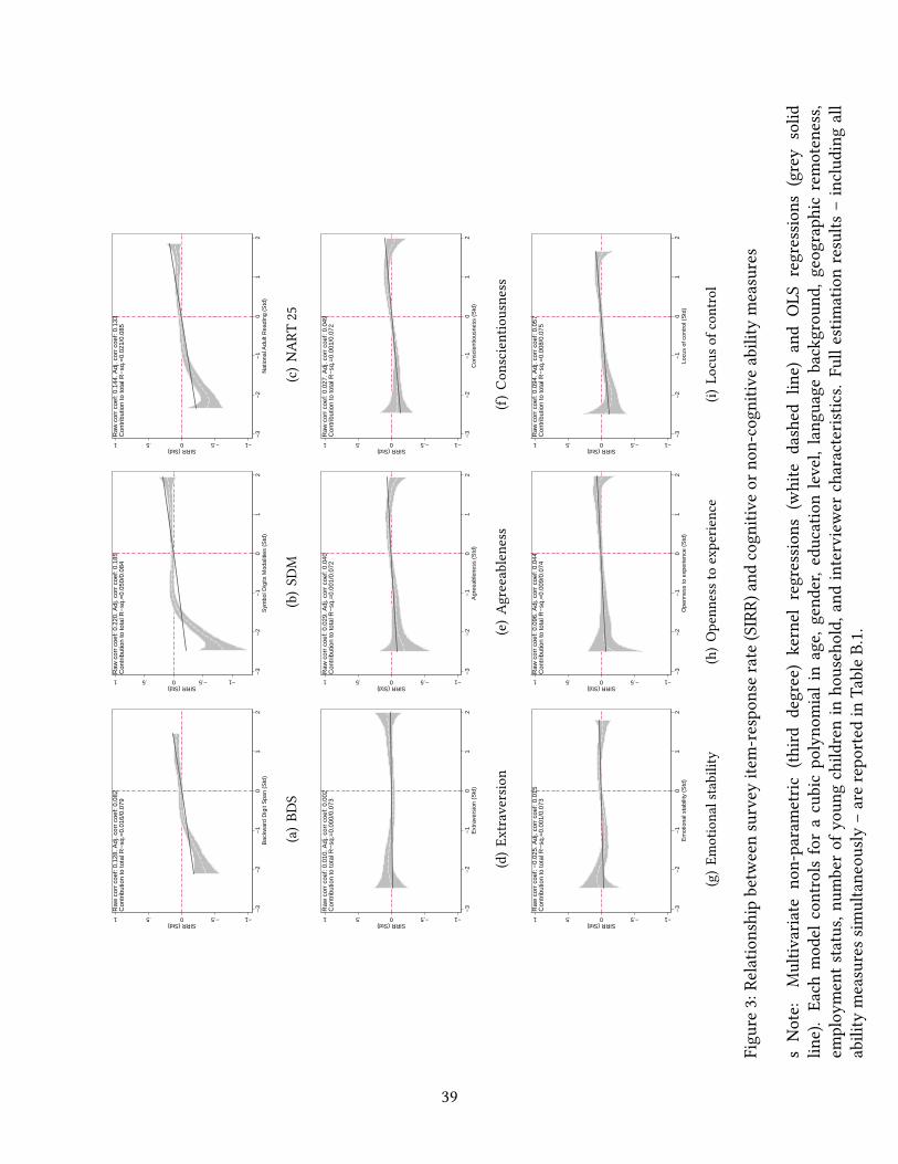
−1−.50.51SIRR (Std)

−3

−2

−1

01

2B

ackw

ard

Dig

it S

pan

(Std

)

Raw

cor

r co

ef: 0

.128

. Adj

. cor

r co

ef: 0

.082

Con

trib

utio

n to

tota

l R−

sq.=

0.01

6/0.

079

(a)BD

S

−1−.50.51SIRR (Std)

−3

−2

−1

01

2S

ymbo

l Dig

its M

odal

ities

(S

td)

Raw

cor

r co

ef: 0

.220

. Adj

. cor

r co

ef: 0

.185

Con

trib

utio

n to

tota

l R−

sq.=

0.05

0/0.

084

(b)SD

M

−1−.50.51SIRR (Std)

−3

−2

−1

01

2N

atio

nal A

dult

Rea

ding

(S

td)

Raw

cor

r co

ef: 0

.144

. Adj

. cor

r co

ef: 0

.133

Con

trib

utio

n to

tota

l R−

sq.=

0.02

1/0.

085

(c)NART

25

−1−.50.51SIRR (Std)

−3

−2

−1

01

2E

xtra

vers

ion

(Std

)

Raw

cor

r co

ef: 0

.010

. Adj

. cor

r co

ef: 0

.002

Con

trib

utio

n to

tota

l R−

sq.=

0.00

0/0.

073

(d)Ex

traversion

−1−.50.51SIRR (Std)

−3

−2

−1

01

2A

gree

able

ness

(S

td)

Raw

cor

r co

ef: 0

.029

. Adj

. cor

r co

ef: 0

.040

Con

trib

utio

n to

tota

l R−

sq.=

0.00

1/0.

072

(e)Agreeableness

−1−.50.51SIRR (Std)

−3

−2

−1

01

2C

onsc

ient

ious

ness

(S

td)

Raw

cor

r co

ef: 0

.027

. Adj

. cor

r co

ef: 0

.049

Con

trib

utio

n to

tota

l R−

sq.=

0.00

1/0.

072

(f)Co

nscientio

usness

−1−.50.51SIRR (Std)

−3

−2

−1

01

2E

mot

iona

l sta

bilit

y (S

td)

Raw

cor

r co

ef: −

0.02

5. A

dj. c

orr

coef

: 0.0

15C

ontr

ibut

ion

to to

tal R

−sq

.=0.

001/

0.07

3

(g)Em

otionalstability

−1−.50.51SIRR (Std)

−3

−2

−1

01

2O

penn

ess

to e

xper

ienc

e (S

td)

Raw

cor

r co

ef: 0

.096

. Adj

. cor

r co

ef: 0

.044

Con

trib

utio

n to

tota

l R−

sq.=

0.00

9/0.

074

(h)Openn

esstoexperie

nce

−1−.50.51SIRR (Std)

−3

−2

−1

01

2Lo

cus

of c

ontr

ol (

Std

)

Raw

cor

r co

ef: 0

.094

. Adj

. cor

r co

ef: 0

.057

Con

trib

utio

n to

tota

l R−

sq.=

0.00

8/0.

075

(i)Lo

cuso

fcon

trol

Figu

re3:Re

latio

nshipbetw

eensurvey

item-respo

nserate

(SIRR)

andcogn

itive

orno

n-cogn

itive

ability

measures

sNote:

Multiv

ariate

non-parametric

(third

degree)kernel

regression

s(w

hite

dashed

line)

and

OLS

regression

s(grey

solid

line).Ea

chmod

elcontrols

foracubicpo

lyno

mialinage,

gend

er,e

ducatio

nlevel,lang

uage

backgrou

nd,g

eographicremoteness,

employ

ments

tatus,nu

mberof

youn

gchild

renin

household,

andinterviewer

characteris

tics.

Fullestim

ationresults

–includ

ingall

ability

measuress

imultaneou

sly–arerepo

rted

inTa

bleB.1.

39

0.0

5.1

.15

.2.2

5.3

.35

.4.4

5.5

Inte

rtem

pora

l cor

rela

tion

coef

ficie

nt

2 3 4 5 6 7 8 9 10 11 12 13Waves

Wave 1 Wave 4 Wave 8 Wave 10

Figure 4: Average inter-temporal correlation coefficient (ITC) of SIRR across waves. Sample:individuals who stayed from wave 1 to 13 in the longitudinal survey (N=4,981)

40

Multicollinearity potential

05

1015

1La

mbd

a

−.5 0 .5 1 1.5 2 2.5 3Relative strength of proxy variable (Strength/POVB)

.05 .20 .40

.60 .80

Figure 5: Simulation of lambda for five different values of the degree of the potential of mul-ticollinearity problem (PMCP). The horizontal axis measures the relative strength of the proxyvariable. A negative sign of the relative strength indicates a violation of the necessary conditionof a valid proxy variable.

41

−4

−3

−2

−1

01

23

4B

ias

redu

ctio

n in

yea

rs o

f edu

catio

n (*

100)

−5 0 5 10 15 20Difference in cognitive ability between respondents and non−respondents

p−value<0.05p−value >= 0.05slope = .47

Figure 6: Scatter plot of percent bias reduction in coefficients on returns to education by differencein cognitive ability between respondents and non-respondents. Cognitive ability is measuredwith Symbol Digits Modalities test

42

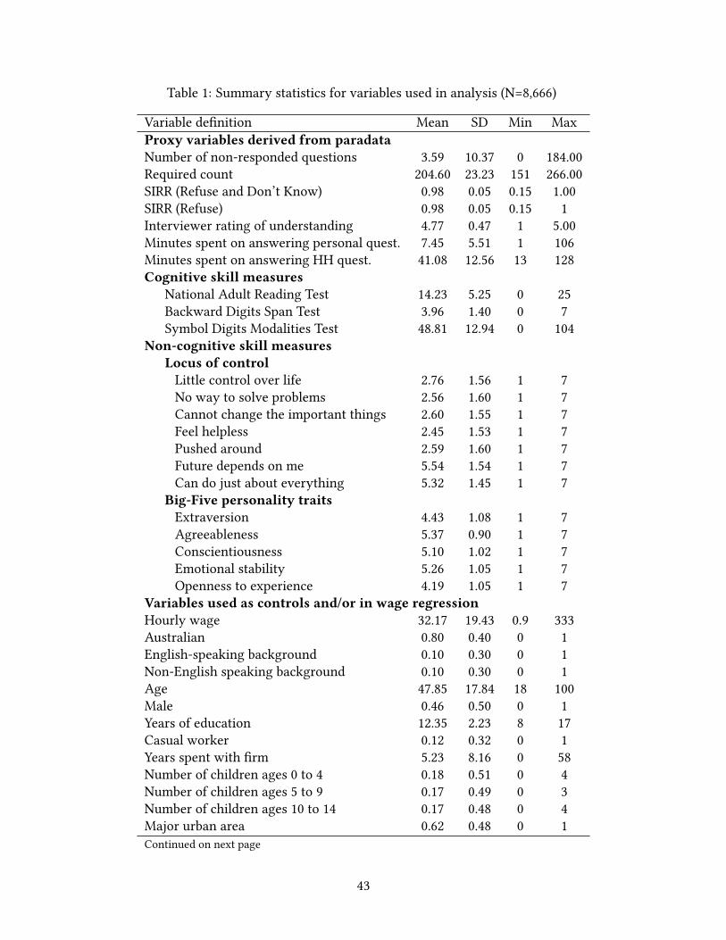
Table 1: Summary statistics for variables used in analysis (N=8,666)

Variable definition Mean SD Min MaxProxy variables derived from paradataNumber of non-responded questions 3.59 10.37 0 184.00Required count 204.60 23.23 151 266.00SIRR (Refuse and Don’t Know) 0.98 0.05 0.15 1.00SIRR (Refuse) 0.98 0.05 0.15 1Interviewer rating of understanding 4.77 0.47 1 5.00Minutes spent on answering personal quest. 7.45 5.51 1 106Minutes spent on answering HH quest. 41.08 12.56 13 128Cognitive skill measures

National Adult Reading Test 14.23 5.25 0 25Backward Digits Span Test 3.96 1.40 0 7Symbol Digits Modalities Test 48.81 12.94 0 104

Non-cognitive skill measuresLocus of controlLittle control over life 2.76 1.56 1 7No way to solve problems 2.56 1.60 1 7Cannot change the important things 2.60 1.55 1 7Feel helpless 2.45 1.53 1 7Pushed around 2.59 1.60 1 7Future depends on me 5.54 1.54 1 7Can do just about everything 5.32 1.45 1 7

Big-Five personality traitsExtraversion 4.43 1.08 1 7Agreeableness 5.37 0.90 1 7Conscientiousness 5.10 1.02 1 7Emotional stability 5.26 1.05 1 7Openness to experience 4.19 1.05 1 7

Variables used as controls and/or in wage regressionHourly wage 32.17 19.43 0.9 333Australian 0.80 0.40 0 1English-speaking background 0.10 0.30 0 1Non-English speaking background 0.10 0.30 0 1Age 47.85 17.84 18 100Male 0.46 0.50 0 1Years of education 12.35 2.23 8 17Casual worker 0.12 0.32 0 1Years spent with firm 5.23 8.16 0 58Number of children ages 0 to 4 0.18 0.51 0 4Number of children ages 5 to 9 0.17 0.49 0 3Number of children ages 10 to 14 0.17 0.48 0 4Major urban area 0.62 0.48 0 1Continued on next page

43

Table 1: Summary statistics for variables used in analysis (N=8,666)

Variable definition Mean SD Min MaxOther urban area 0.22 0.42 0 1Bounded locality 0.03 0.16 0 1Rural balance 0.13 0.33 0 1New South Wales 0.29 0.46 0 1Victoria 0.25 0.43 0 1Queensland 0.21 0.41 0 1South Australia 0.09 0.28 0 1Western Australia 0.10 0.29 0 1Tasmania 0.03 0.17 0 1Northern Territory 0.01 0.08 0 1Australian Capital Territory 0.02 0.15 0 1

44

Table2:Predictiv

epo

wer

ofSIRR

Logho

urly

wages

Highscho

olHealth

(-0.1,6.1)

(0,1)

(0,100)

Includ

ing

Includ

ing

Includ

ing

Includ

ing

Includ

ing

Includ

ing

SIRR

CS&SIRR

SIRR

CS&SIRR

SIRR

CS&SIRR

(1)

(2)

(3)

(4)

(5)

(6)

SIRR

(Std)

0.0262**

0.0155

0.0297***

0.00573

0.606**

0.313

(0.0114)

(0.0115)

(0.00527)

(0.00512)

(0.259)

(0.262)

Symbo

lDigits

Mod

alities

(Std)

0.0485***

0.0345***

1.744***

(0.0103)

(0.00605)

(0.283)

NationalA

dultRe

ading(Std)

0.0425***

0.130***

0.571**

(0.00918)

(0.00538)

(0.262)

BackwardDigitSp

an(Std)

0.00262

0.00778

-0.259

(0.00719)

(0.00481)

(0.222)

Observatio

ns5780

5780

8666

8666

8588

8588

AdjustedR2

1110

1165

0.123

0.203

0.252

0.256

Note:Dependent

varia

bles

arelog

hourlywages

(mod

els1

,2),high

scho

oldegree

(mod

els3

,4)and

SF-36generalhealth

compo

nent

(Mod

els5

,6).Mod

els(1)and(2)are

estim

ated

with

aTo

bitsam

pleselectionmod

el,w

ithleftcensored

observations

settomissing

.Ex

clusionrestric

tionfors

electio

nequatio

narenu

mbero

fchildrenin

agebracket0

-4,5-10,11-14.Th

eMillsr

atio

is0.05

(t-value

of1.1)

formod

el(1)a

nd0.08

(t-valueof

1.6)

formod

el(2).Estim

ationsamples

inmod

els(1)a

nd(2)a

rebasedon

working

age

popu

latio

n,ages

24to

64.A

llotherm

odelsa

reestim

ated

with

OLS

with

noagerestric

tion.

Mod

els3

and4arelin

earp

robability

mod

els.Allregression

mod

elsc

ontrol

forg

ender,age,yearso

fedu

catio

n(exceptm

odels(2)

and(3)),

adu

mmyforc

asualw

orker,

yearso

ftenurewith

currentfi

rmandits

square,stateof

residencedu

mmies,region

dummies(otheru

rban,bou

nded

locality,rural

balance),langu

agebackgrou

nd,B

ig5person

ality

traits.M

odels(3)and(4)add

ition

allycontrolfor

labo

rforce

status

(unemploy

ed,

outo

fthe

labo

rforce).Standard

errors

arerepo

rted

inparentheses.*p

<0.10,**p

<0.05,***p<

0.01.

45

Table 3: Estimates of λ and percent bias reduction

Education Locus of(Years) control (Std)

Panel A: Partial correlation coefficients1. Strength of proxy variable: rMP|Z 0.117 0.1172. Omitted-variable potential: rXM|Z 0.144 0.0703. Multicollinearity potential: rXP|Z 0.128 0.0404. Relative strength of proxy variable: rMP|Z

rXM|Z0.810 1.675

5. Ratio of the squared biases: λa 0.830 0.873Panel B: Bias reduction in percent of omitted-variable biasb

1. Linear SIRR (N=5,780) 8.9*** 6.5***2. Non-linear SIRRc (N=5,780) 10.1*** 7.3***3. SIRR based on refusals only (N=5,780) 7.9*** 5.6***4. Age range 20-69 sample (N=7,215) 10.0*** 8.3***5. Drop if SIRR <= 0.4 (N=5,771) 10.3*** 7.2***6. Drop Non-Engl. background (N=5,183) 10.2*** 6.3***7. Alternative CA: BDS (N=5,780) 5.4*** 11.4***8. Alternative CA: NART 25 (N=5,780) 2.7*** 5.6***

Note: rMP|Z rXP|Z and rXM|Z are the partial correlation coefficients of cognitiveskills M and the proxy variable P (strength of proxy), of the education or locus ofcontrol variable X and the proxy variable P (multicollinearity potential), and of theeducation or non-cognitive skill variable X and cognitive skills M (omitted-variablepotential), netting out the effect of all other control variables used in the wage re-gression model. a λ measures the squared relative bias, and stars measure the nullhypothesis that the ratio is equal to one, against the alternative hypothesis that theratio is smaller than 1. b Bias reduction is calculated as the percentage change in theomitted-variable bias, calculated as: (OVB−IPB)

OVB×100. Standard errors for λ and the

bias reduction are calculated with the delta method. c Non-linear measure of SIRRis captured by four dummy variables that indicate non-response rates within the 5thpercentile, between the 5th and 10th percentile, between the 10th and 25th percentile,and above the 25th percentile. The comparison group is zero non-response. * p<0.10** p<0.05, *** p<0.01.

46

Table 4: Relative performance of SIRR as proxy variable for cognitive skills against alter-native proxy variables

Proxy variable (Std) Years Education Locus of controlλa BRb λ BR

1. Survey item response 0.83 8.9*** 0.87 6.5***2. Interviewer rating understanding 0.88 6.1*** 0.77 12.5***3. Minutes spent on personal questionnaire 0.99 0.53 1.00 -0.054. Minutes spend on household questionnaire 0.98 1.2 0.90 4.9***5. Days elapsed until SCQ returned 1.23 -11.2*** 1.60 -26.5***

Note: All proxy variables are standardised to mean 0 and standard deviation 1. Alternative proxy vari-ables derived from para data are: 2. Interviewer rating of the understanding of questions; 3. Minutesspent on completing personal questionnaires; 4. Minutes spent on completing the household ques-tionnaire; 5. Days elapsed between receiving and completing the self-completion questionnaires. a

λ measures the squared relative bias, and stars measure the null hypothesis that the ratio is equal toone, against the alternative hypothesis that the ratio is smaller than 1. a Bias reduction is calculatedas the percentage change in the omitted-variable bias, calculated as: (OVB−IPB)

OVB× 100.

47

Table 5: Bias-adjusted wage returns to education under various assumptions

True effect β∗ β∗+OVB Oster (2017) method β∗+IPB(Full (Omitting R2

max = 1.3R2 R2max = 1 (Including

model) Cogn. Ability) δ = 1 δ = 1 SIRR)(1) (2) (3) (4) (5)

β 0.0763 0.0790 0.0741 -0.5919 0.0782

Note: All models are estimated with 4,024 working individuals with positive hourly wages in Wave 12. Thedependent variable is log hourly wages. Reported are the coefficients (labeled "β") for years of education fromOLS models. All regression models control for gender, age, years of education, a dummy for casual worker,years of tenure with current firm and its square, state of residence dummies, region dummies (other urban,bounded locality, rural balance), language background, Big-5 personality traits. Model (1) additionally controlsfor cognitive ability and shows the true effect of education (β∗) under the assumption that all relevant variablesare controlled for. Model (2) shows the effect of educationwhen cognitive skills are omitted and thus the estimatesuffers from omitted-variable bias (OVB). Models (3) and (4) show the bias adjusted effects as suggested by Oster(2017). Model (3) shows the effect assuming that the degree of selection on unobservables is equal the degree ofselection on observables (δ = 1) and the maximum R-squared that can be achieved is 1.3 times the R-Squared ofModel (2) (Rmax = 1.3 ∗ 0.22 = 0.29) as suggested in Oster (2017). Model (4) assumes δ = 1, but a maximumR-squared of 1. Model (5) controls for SIRR and therefore shows an effect that potentially includes an imperfectproxy bias. The calculation of the bias adjusted effects are based on the STATA command psacalc written byEmily Oster and available through ssc.

48

ARespo

nsebe

havior

onself-com

pletionqu

estion

nairein

unrestricted

sample

TableA.1:Q

uestions

andno

n-respon

se

Varia

blein

SCQ:

NR

DK

Ref

Bias

redu

ction

NOrdered

bylargesttosm

allestno

n-respon

seprop

ortio

n(%)

(%)

(%)

ReturnstoEd

ucation

SCQ:B23m

How

long

agolifeeventh

appened-Jailed-n

oansw

er0.816

00.816

1.801

174

SCQ:B23cHow

long

agolifeeventh

appened-R

econ

ciled-n

oansw

er0.578

00.578

1.045

287

SCQ:B23hHow

long

agolifeeventh

appened-D

eath

ofspou

se/child

-noansw

er0.575

00.575

2.069

322

SCQ:B23oHow

long

agolifeeventh

appened-R

etire

d-n

oansw

er0.499

00.499

1.037

557

SCQ:B23vHow

long

agolifeeventh

appened-H

omedestroyed-n

oansw

er0.483

00.483

0.876

362

SCQ:B23nHow

long

agolifeeventh

appened-F

amily

mem

berjailed-n

oansw

er0.473

00.473

1.677

391

SCQ:B23kHow

long

agolifeeventh

appened-V

ictim

ofviolence

-noansw

er0.467

00.467

2.333

407

SCQ:B23tH

owlong

agolifeeventh

appened-F

inancialworsening

-noansw

er0.371

00.371

1.669

590

SCQ:D3b

Workp

lace

entitlements:P

aidpaternity

leave

0.335

0.326

0.008

-2.539

9485

SCQ:B23pHow

long

agolifeeventh

appened-F

ired-n

oansw

er0.329

00.329

1.568

645

SCQ:B23sH

owlong

agolifeeventh

appened-F

inancialim

provem

ent-

noansw

er0.311

00.311

0.924

601

SCQ:B23aHow

long

agolifeeventh

appened-M

arrie

d-n

oansw

er0.289

00.289

1.163

494

SCQ:B23rH

owlong

agolifeeventh

appened-P

romoted

-noansw

er0.266

00.266

0.151

1121

SCQ:B23eHow

long

agolifeeventh

appened-G

ainedfamily

-noansw

er0.259

00.259

0.501

746

SCQ:D3a

Workp

lace

entitlements:P

aidmaternity

leave

0.255

0.248

0.008

-2.229

9485

SCQ:B23bHow

long

agolifeeventh

appened-S

eparated

-noansw

er0.254

00.254

1.975

700

SCQ:B23lH

owlong

agolifeeventh

appened-V

ictim

ofprop

erty

crim

e-n

oansw

er0.248

00.248

1.348

738

SCQ:D3c

Workp

lace

entitlements:S

pecialleaveforc

aringforfam

ilymem

bers

0.216

0.208

0.008

-0.546

9485

SCQ:D3g

Child

care

facilitieso

rsub

sidisedchild

care

expenses

0.211

0.201

0.01

-1.363

9485

SCQ:B23dHow

long

agolifeeventh

appened-P

regn

ancy

-noansw

er0.205

00.205

0.170

980

SCQ:B23jH

owlong

agolifeeventh

appened-D

eath

offriend

-noansw

er0.205

00.205

1.010

2029

SCQ:B23fH

owlong

agolifeeventh

appened-Injuryto

self-n

oansw

er0.191

00.191

0.452

1594

SCQ:B23gHow

long

agolifeeventh

appened-Injuryto

relativ

e/family

-noansw

e0.153

00.153

0.919

2676

SCQ:D3d

Workp

lace

entitlements:P

ermanentp

art-tim

ework

0.151

0.142

0.009

-0.941

9485

SCQ:D3e

Workp

lace

entitlements:H

ome-basedwork

0.148

0.138

0.01

-0.152

9485

SCQ:B23iH

owlong

agolifeeventh

appened-D

eath

ofotherrel-n

oansw

er0.146

00.146

1.042

2180

SCQ:B23qHow

long

agolifeeventh

appened-C

hang

edjobs

-noansw

er0.146

00.146

0.277

2159

SCQ:C6b

Financialrisk-a

ssum

ed0.139

00.139

1.719

2755

SCQ:B23uHow

long

agolifeeventh

appened-M

oved

-noansw

er0.123

00.123

0.681

2635

SCQ:B12bNeigh

bourho

od:N

eigh

boursd

oing

things

together

0.117

0.11

0.006

-0.430

15380

SCQ:B24iH

ours

perw

eek-C

aringford

isabledspou

se/relative

0.104

00.104

1.440

15380

SCQ:B24iM

inutes

perw

eek-C

aringford

isabledspou

se/relative

0.104

00.104

1.440

15380

SCQ:B12aNeigh

bourho

od:N

eigh

boursh

elping

each

othero

ut0.1

0.095

0.005

-0.592

15380

SCQ:B13dSatisfactionwith

:Relationshipwith

step

child

ren

0.099

00.099

2.199

2191

SCQ:B24gHou

rsperw

eek-P

laying

with

otherc

hildren

0.098

00.098

1.690

15380

SCQ:B24gMinutes

perw

eek-P

laying

with

otherc

hildren

0.098

00.098

1.690

15380

SCQ:B24hHou

rsperw

eek-V

olun

teer/Charitywork

0.093

00.093

2.576

15380

SCQ:B24hMinutes

perw

eek-V

olun

teer/Charitywork

0.093

00.093

2.576

15380

SCQ:B12jN

eigh

bourho

od:B

urglaryandtheft

0.092

0.087

0.006

-0.265

15380

SCQ:B13gSatisfactionwith

:Relationshipwith

step

parents

0.088

00.088

2.054

2683

Continuedon

next

page

49

TableA.1:Q

uestions

andno

n-respon

se

Varia

blein

SCQ:

NR

DK

Ref

Bias

redu

ction

NOrdered

bylargesttosm

allestno

n-respon

seprop

ortio

n(%)

(%)

(%)

ReturnstoEd

ucation

SCQ:D3f

Workp

lace

entitlements:F

lexiblestart/fi

nish

times

0.085

0.077

0.008

0.746

9485

SCQ:B3Num

bero

fcigarettesu

sually

smok

edeach

week

0.077

00.077

1.027

2933

SCQ:B24fH

ours

perw

eek-P

laying

with

your

child

ren

0.076

00.076

2.689

15380

SCQ:B24fM

inutes

perw

eek-P

laying

with

your

child

ren

0.076

00.076

2.689

15380

SCQ:C2b

Couldno

tpay

themortgageor

rent

ontim

e0.062

00.062

1.205

15380

SCQ:C2c

Pawnedor

sold

something

0.06

00.06

1.019

15380

SCQ:C2e

Was

unableto

heat

home

0.06

00.06

1.241

15380

SCQ:C2g

Asked

forh

elpfrom

welfare/com

mun

ityorganisatio

ns0.06

00.06

0.985

15380

SCQ:C2d

Wentw

ithou

tmeals

0.059

00.059

1.054

15380

SCQ:C2a

Couldno

tpay

electricity

,gas

orteleph

onebills

ontim

e0.057

00.057

0.918

15380

SCQ:C2f

Asked

forfi

nancialh

elpfrom

friend

sorfam

ily0.057

00.057

1.021

15380

SCQ:C9iMon

thly

householdexpend

iture

-Childrens

clothing

andfootwear

0.052

00.052

1.685

10477

SCQ:C9d

Weeklyho

useholdexpend

iture

-Pub

lictransporta

ndtaxis

0.05

00.05

1.133

10477

SCQ:C7e

Hou

seho

lddecision

s-Th

eway

child

renareraised

0.048

00.048

2.169

6714

SCQ:C9c

Weeklyho

useholdexpend

iture

-Cigarettesa

ndtobacco

0.047

00.047

0.520

10477

SCQ:B24bHou

rsperw

eek-T

ravelling

toandfrom

aplaceof

paid

employ

ment

0.046

00.046

2.131

15380

SCQ:B24bMinutes

perw

eek-T

ravelling

toandfrom

aplaceof

paid

employ

ment

0.046

00.046

2.131

15380

SCQ:C9h

Mon

thly

householdexpend

iture

-Wom

ensc

lothingandfootwear

0.043

00.043

1.504

10477

SCQ:B25gCo

mpu

teru

se-C

ompu

ters

have

helped

mereachmyoccupatio

nal(career)

0.042

00.042

2.401

15380

SCQ:B13hSatisfactionwith

:Relationshipwith

mostrecentformer

spou

se/partner

0.041

00.041

0.930

4689

SCQ:B24eHou

rsperw

eek-O

utdo

ortasks

0.041

00.041

1.548

15380

SCQ:B24eMinutes

perw

eek-O

utdo

ortasks

0.041

00.041

1.548

15380

SCQ:C9g

Mon

thly

householdexpend

iture

-Mensc

lothingandfootwear

0.041

00.041

1.053

10477

SCQ:C9p

Ann

ualh

ouseho

ldexpend

iture

-Hom

erepairs

/renovations/m

aintenance

0.041

00.041

0.994

10477

SCQ:C9r

Ann

ualh

ouseho

ldexpend

iture

-Edu

catio

nfees

0.041

00.041

1.620

10477

SCQ:B24cHou

rsperw

eek-H

ouseho

lderrand

s0.04

00.04

3.306

15380

SCQ:B24cMinutes

perw

eek-H

ouseho

lderrand

s0.04

00.04

3.306

15380

SCQ:C7d

Hou

seho

lddecision

s-Th

enu

mbero

fhou

rsyo

urpartner/spou

sespends

in0.04

00.04

2.024

8298

SCQ:B25cCo

mpu

teru

se-C

ompu

ters

have

madeitpo

ssibleform

eto

getm

oredo

ne0.039

00.039

2.689

15380

SCQ:B25eCo

mpu

teru

se-C

ompu

ters

have

helped

meto

learnnewskillso

ther

than

0.039

00.039

2.992

15380

SCQ:B25fC

ompu

teru

se-C

ompu

ters

have

helped

meto

commun

icatewith

peop

le0.039

00.039

2.524

15380

SCQ:B25aCo

mpu

teru

se-M

ylevelo

fcom

puters

kills

meetsmypresentn

eeds

0.038

00.038

3.018

15380

SCQ:B25dCo

mpu

teru

se-C

ompu

ters

have

madeiteasier

form

eto

getu

sefulinfor

0.038

00.038

2.658

15380

SCQ:C9b

Weeklyho

useholdexpend

iture

-Alcoh

ol0.038

00.038

0.824

10477

SCQ:B25bCo

mpu

teru

se-I

feelcomfortableinstallin

gor

upgradingcompu

ters

oft

0.037

00.037

2.669

15380

SCQ:B12hNeigh

bourho

od:P

eoplebeingho

stile

andaggressive

0.036

0.029

0.006

0.269

15380

SCQ:B12iN

eigh

bourho

od:V

andalism

anddelib

eratedamageto

prop

erty

0.035

0.03

0.005

-0.163

15380

SCQ:B14aTh

eway

child

care

tasksa

redividedbetw

eenyo

uandyo

urpartner

0.035

00.035

1.258

4927

SCQ:B24aHou

rsperw

eek-P

aidem

ploy

ment

0.035

00.035

2.325

15380

SCQ:B24aMinutes

perw

eek-P

aidem

ploy

ment

0.035

00.035

2.325

15380

SCQ:C9m

Ann

ualh

ouseho

ldexpend

iture

-Feesp

aidto

health

practitioners

0.034

00.034

1.229

10477

SCQ:C9lAnn

ualh

ouseho

ldexpend

iture

-Other

insurance(hom

e/contents/m

otor

vehi

0.033

00.033

1.212

10477

SCQ:C9o

Ann

ualh

ouseho

ldexpend

iture

-Electric

itybills,gas

bills

andotherh

e0.033

00.033

1.164

10477

SCQ:B12eNeigh

bourho

od:H

omes

andgardensinbadcond

ition

0.031

0.025

0.006

0.812

15380

Continuedon

next

page

50

TableA.1:Q

uestions

andno

n-respon

se

Varia

blein

SCQ:

NR

DK

Ref

Bias

redu

ction

NOrdered

bylargesttosm

allestno

n-respon

seprop

ortio

n(%)

(%)

(%)

ReturnstoEd

ucation

SCQ:C9q

Ann

ualh

ouseho

ldexpend

iture

-Motor

vehiclerepairs

/maintenance

0.031

00.031

1.078

10477

SCQ:B13eSatisfactionwith

:Childrenin

householdgeta

long

with

each

other

0.03

00.03

1.220

6195

SCQ:C9n

Ann

ualh

ouseho

ldexpend

iture

-Medicines,prescrip

tions,pharm

aceutic

als

0.03

00.03

0.739

10477

SCQ:B24dHou

rsperw

eek-H

ousework

0.029

00.029

2.724

15380

SCQ:B24dMinutes

perw

eek-H

ousework

0.029

00.029

2.724

15380

SCQ:C9e

Weeklyho

useholdexpend

iture

-Mealseatenou

t0.029

00.029

0.987

10477

DV:[SC

Q:B]H

eigh

tincentim

etres

0.029

00.029

0.346

15380

SCQ:C7c

Hou

seho

lddecision

s-Th

enu

mbero

fhou

rsyo

uspendin

paid

work

0.028

00.028

1.494

10728

SCQ:C9jMon

thly

householdexpend

iture

-Telepho

nerent,callsandinternet

charg

0.028

00.028

1.228

10477

SCQ:C9f

Mon

thly

householdexpend

iture

-Motor

vehiclefuel

0.027

00.027

1.102

10477

SCQ:C9k

Ann

ualh

ouseho

ldexpend

iture

-Priv

atehealth

insurance

0.026

00.026

1.292

10477

SCQ:B12gNeigh

bourho

od:T

eenagers

hang

ingarou

ndon

thestreets

0.025

0.019

0.006

0.580

15380

SCQ:B17cTo

whate

xtenth

asyo

urrelatio

nshipmet

your

originalexpectations

0.025

00.025

0.888

9866

DV:[SC

Q:B]W

eigh

tinkilogram

s0.025

00.025

0.821

15380

SCQ:C3a

Diffi

culty

inraising(w

aves

1-8)

2,000(w

aves9+)3,000

fora

nem

erge

0.024

00.024

0.639

15380

SCQ:B17aHow

good

isyo

urrelatio

nshipcomparedto

most

0.023

00.023

1.129

9866

SCQ:B17dHow

muchdo

youlove

your

spou

se/partner

0.023

00.023

0.760

9866

SCQ:B17fH

owwelld

oesy

ours

pousemeety

ourn

eeds

0.023

00.023

0.765

9866

SCQ:B18

Shareof

workarou

ndtheho

use

0.023

00.023

1.203

15380

SCQ:C4Saving

shabits

0.023

00.023

0.925

15380

SCQ:C6a

Financialriskprepared

totake

0.023

00.023

1.698

15380

SCQ:B17bHow

oftendo

youwishyo

uhadno

tgot

marrie

d/g

otinto

thisrelatio

ns0.022

00.022

0.952

9866

SCQ:B17eHow

manyproblemsa

retherein

your

relatio

nship

0.022

00.022

0.848

9866

SCQ:C7g

Hou

seho

lddecision

s-Saving

s,investmenta

ndbo

rrow

ing

0.022

00.022

1.852

13562

SCQ:C9a

Weeklyho

useholdexpend

iture

-Grocerie

s0.022

00.022

0.845

10476

SCQ:E1Has

parentingrespon

sibilitiesfor

anychild

renaged

17yearso

rless

0.022

00.022

1.451

15380

SCQ:C3b

How

wou

ldobtain

(waves

1-8)

2,000(w

aves9+)3,000

-NoAnswer

0.022

00.022

1.290

13385

SCQ:C7f

Hou

seho

lddecision

s-Sociallifeandleisureactiv

ities

0.021

00.021

1.472

14129

SCQ:B13cSatisfactionwith

:Partnersr

elationshipwith

child

ren

0.019

00.019

1.803

8181

SCQ:C5Mostimpo

rtantw

henplanning

saving

sand

spending

0.019

00.019

0.999

15380

SCQ:C7b

Hou

seho

lddecision

s-Makinglargeho

useholdpu

rchases

0.018

00.018

1.060

13845

SCQ:B12cNeigh

bourho

od:T

rafficno

ise

0.017

0.007

0.01

0.873

15380

SCQ:B12fN

eigh

bourho

od:R

ubbish

andlitterlying

arou

nd0.017

0.011

0.006

0.956

15380

SCQ:B14bTh

eway

householdtasksa

redividedbetw

eenyo

uandyo

urpartner

0.017

00.017

1.621

10028

SCQ:C7a

Hou

seho

lddecision

s-Managingday-to-day

spending

andpaying

bills

0.016

00.016

1.114

14234

SCQ:B12dNeigh

bourho

od:N

oise

from

airplanes,trains

orindu

stry

0.015

0.009

0.007

1.214

15380

SCQ:B13fS

atisfactionwith

:Relationshipwith

parents

0.015

00.015

1.682

10811

SCQ:B19

How

oftengettog

ethers

ocially

with

friend

s/relativ

esno

tlivingwith

y0.015

00.015

1.415

15380

SCQ:E4jWork-family

balance:Myworkhasa

positiv

eeff

ecto

nmychild

ren

0.015

00.015

0.025

3510

SCQ:E4m

Work-family

balance:Worry

abou

tchildrenwhileat

work

0.015

00.015

-0.102

3510

SCQ:B5Standard

drinks

usually

have

perd

ay0.014

00.014

0.277

12538

SCQ:B21cAchievementm

otivation-I

feelun

easy

abou

tund

ertaking

atask

ifIa

0.014

00.014

1.332

15380

SCQ:E4c

Work-family

balance:Workmakes

mefeelcompetent

0.014

00.014

0.026

3510

SCQ:E4e

Work-family

balance:Havingbo

thworkandfamily

respon

sibilitiesc

halle

0.014

00.014

0.121

3510

Continuedon

next

page

51

TableA.1:Q

uestions

andno

n-respon

se

Varia

blein

SCQ:

NR

DK

Ref

Bias

redu

ction

NOrdered

bylargesttosm

allestno

n-respon

seprop

ortio

n(%)

(%)

(%)

ReturnstoEd

ucation

SCQ:E4f

Work-family

balance:Timeworking

less

enjoyable/morepressured

0.014

00.014

-0.025

3510

SCQ:E4iWork-family

balance:Working

makes

mefeelgo

odabou

tmyself,which

isg

0.014

00.014

0.058

3510

SCQ:E4k

Work-family

balance:Be

ttera

ppreciatetim

espentw

ithchild

ren

0.014

00.014

-0.002

3510

SCQ:E4lWork-family

balance:Working

makes

meabette

rparent

0.014

00.014

0.021

3510

SCQ:E4p

Work-family

balance:Th

inking

abou

tthe

child

reninterferes

with

myperf

0.014

00.014

0.058

3510

SCQ:A3iPh

ysicalFu

nctio

ning

:Walking

100metres

0.013

00.013

0.627

15380

SCQ:A4c

Role-phy

sical:Werelim

itedin

thekind

ofwork

0.013

00.013

1.721

15380

SCQ:B13aSatisfactionwith

:Partner

0.013

00.013

0.795

10919

SCQ:B13bSatisfactionwith

:Children

0.013

00.013

2.240

10095

SCQ:B21dAchievementm

otivation-W

henconfronted

byadifficultproblem,I

pre

0.013

00.013

1.259

15380

SCQ:B21gAchievementm

otivation-E

venwhenno

body

iswatching,Ifeelanx

ious

0.013

00.013

1.356

15380

SCQ:B21hAchievementm

otivation-I

amattractedto

tasksthata

llowmeto

test

0.013

00.013

1.412

15380

SCQ:B21iA

chievementm

otivation-I

startfeelin

ganxiou

sifI

dono

tund

erstan

0.013

00.013

1.146

15380

SCQ:B23rL

ifeeventsin

pastyear:P

romoted

atwork

0.013

00.013

1.298

15380

SCQ:D1Isin

paid

work

0.013

00.013

1.393

15380

SCQ:E4g

Work-family

balance:Misso

uton

home/family

activ

ities

0.013

00.013

0.005

3510

SCQ:E4h

Work-family

balance:Family

timeless

enjoyable/morepressured

0.013

00.013

0.055

3510

SCQ:E4n

Work-family

balance:To

olittle

timeor

energy

tobe

aspiratio

nalp

arent

0.013

00.013

0.064

3510

SCQ:E4o

Work-family

balance:Misso

uton

therewarding

aspectso

fbeing

parent

0.013

00.013

0.023

3510

SCQ:A3e

PhysicalFu

nctio

ning

:Clim

bing

onefligh

tofstairs

0.012

00.012

1.037

15380

SCQ:B15

Sexu

alIdentity

0.012

00.012

0.360

15380

SCQ:B21bAchievementm

otivation-I

likesituations

where

Ican

findou

thow

ca0.012

00.012

2.015

15380

SCQ:B21eAchievementm

otivation-I

amafraid

oftasksthatI

cann

otworkou

to0.012

00.012

2.435

15380

SCQ:B21fA

chievementm

otivation-I

enjoysituations

that

makeuseof

myabilit

0.012

00.012

1.812

15380

SCQ:E4b

Work-family

balance:Workgivesm

ylifemorevarie

ty0.012

00.012

0.011

3510

SCQ:E4d

Work-family

balance:Haveto

turn

downwork/op

portun

ities

0.012

00.012

0.011

3510

SCQ:A4d

Role-phy

sical:Had

difficulty

performingworkor

othera

ctivities

0.011

00.011

0.337

15380

SCQ:A5c

Role-emotional:Didnt

dowork/othera

ctivities

ascarefully

asusual

0.011

00.011

0.637

15380

SCQ:A11cHealth

:Exp

ectm

yhealth

togetw

orse

0.011

00.011

0.355

15380

SCQ:A11dHealth

:Myhealth

isexcellent

0.011

00.011

0.720

15380

SCQ:B4Drin

kalcoho

l0.011

00.011

0.098

15380

SCQ:B20fT

here

issomeone

who

canalwaysc

heer

meup

whenIm

down

0.011

00.011

1.373

15380

SCQ:B21aAchievementm

otivation-Indifficultsituations

where

alotd

epends

o0.011

00.011

1.447

15380

SCQ:B23gLife

eventsin

pastyear:S

erious

injury/illnesstofamily

mem

ber

0.011

00.011

1.406

15380

SCQ:B23kLife

eventsin

pastyear:V

ictim

ofph

ysicalviolence

0.011

00.011

1.599

15380

SCQ:E4a

Work-family

balance:Workmakes

meamoreroun

dedperson

0.011

00.011

0.011

3510

SCQ:A3a

PhysicalFu

nctio

ning

:Vigorou

sactivities

0.01

00.01

0.242

15380

SCQ:A3d

PhysicalFu

nctio

ning

:Clim

bing

severalfl

ightso

fstairs

0.01

00.01

0.753

15380

SCQ:A3f

PhysicalFu

nctio

ning

:Bending

kneelin

gor

stoo

ping

0.01

00.01

0.666

15380

SCQ:A3h

PhysicalFu

nctio

ning

:Walking

halfakilometre

0.01

00.01

0.502

15380

SCQ:A4b

Role-phy

sical:Accom

plishedless

than

wou

ldlik

e0.01

00.01

0.634

15380

SCQ:A11aHealth

:Get

sick

alittle

easier

than

otherp

eople

0.01

00.01

0.576

15380

SCQ:A11bHealth

:Ash

ealth

yas

anyb

odyIk

now

0.01

00.01

1.088

15380

SCQ:B16

Marrie

dor

inalong

-term

relatio

nship

0.01

00.01

1.007

15380

Continuedon

next

page

52

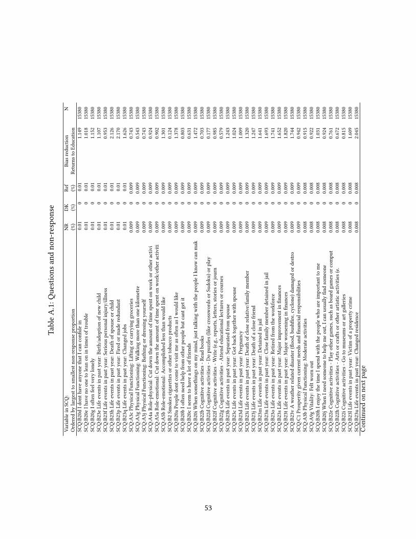
TableA.1:Q

uestions

andno

n-respon

se

Varia

blein

SCQ:

NR

DK

Ref

Bias

redu

ction

NOrdered

bylargesttosm

allestno

n-respon

seprop

ortio

n(%)

(%)

(%)

ReturnstoEd

ucation

SCQ:B20dId

onth

aveanyo

nethat

Ican

confi

dein

0.01

00.01

1.149

15380

SCQ:B20eIh

aveno

oneto

lean

onin

times

oftrou

ble

0.01

00.01

1.018

15380

SCQ:B20gIo

ftenfeelvery

lonely

0.01

00.01

1.152

15380

SCQ:B23eLife

eventsin

pastyear:B

irth/adop

tionof

newchild

0.01

00.01

1.107

15380

SCQ:B23fL

ifeeventsin

pastyear:S

erious

person

alinjury/illness

0.01

00.01

0.953

15380

SCQ:B23hLife

eventsin

pastyear:D

eath

ofspou

seor

child

0.01

00.01

2.126

15380

SCQ:B23pLife

eventsin

pastyear:F

iredor

maderedu

ndant

0.01

00.01

2.170

15380

SCQ:B23qLife

eventsin

pastyear:C

hang

edjobs

0.01

00.01

1.626

15380

SCQ:A3c

PhysicalFu

nctio

ning

:Liftingor

carrying

groceries

0.009

00.009

0.743

15380

SCQ:A3g

PhysicalFu

nctio

ning

:Walking

morethan

onekilometre

0.009

00.009

0.543

15380

SCQ:A3jPh

ysicalFu

nctio

ning

:Bathing

ordressing

yourself

0.009

00.009

0.743

15380

SCQ:A4a

Role-phy

sical:Cu

tdow

ntheam

ount

oftim

espento

nworkor

othera

ctivi

0.009

00.009

0.924

15380

SCQ:A5a

Role-emotional:Cu

tdow

ntheam

ount

oftim

espento

nwork/othera

ctiviti

0.009

00.009

0.902

15380

SCQ:A5b

Role-emotional:Accom

plishedless

than

wou

ldlik

e0.009

00.009

1.301

15380

SCQ:B2Sm

okes

cigarette

soro

ther

tobaccoprod

ucts

0.009

00.009

0.124

15380

SCQ:B20aPeop

ledo

ntcometo

visitm

eas

oftenas

Iwou

ldlik

e0.009

00.009

1.378

15380

SCQ:B20bIo

ftenneed

help

from

otherp

eoplebu

tcantg

etit

0.009

00.009

0.803

15380

SCQ:B20cIseem

tohave

aloto

ffrie

nds

0.009

00.009

0.631

15380

SCQ:B20iW

hensomething

sonmymind,justtalkingwith

thepeop

leIk

nowcanmak

0.009

00.009

1.472

15380

SCQ:B22bCo

gnitive

activ

ities

-Readbo

oks

0.009

00.009

0.703

15380

SCQ:B22dCo

gnitive

activ

ities

-Dopu

zzles(lik

ecrossw

ords

orSu

doku

)orp

lay

0.009

00.009

0.177

15380

SCQ:B22fC

ognitiv

eactiv

ities

-Write(e.g.,repo

rts,lette

rs,storie

sorjou

rn0.009

00.009

0.985

15380

SCQ:B22gCo

gnitive

activ

ities

-Atte

ndeducationallectureso

rcou

rses

0.009

00.009

0.579

15380

SCQ:B23bLife

eventsin

pastyear:S

eparated

from

spou

se0.009

00.009

1.243

15380

SCQ:B23cLife

eventsin

pastyear:G

otback

together

with

spou

se0.009

00.009

1.024

15380

SCQ:B23dLife

eventsin

pastyear:P

regn

ancy

0.009

00.009

1.009

15380

SCQ:B23iL

ifeeventsin

pastyear:D

eath

ofcloserelativ

e/family

mem

ber

0.009

00.009

1.320

15380

SCQ:B23jL

ifeeventsin

pastyear:D

eath

ofaclosefriend

0.009

00.009

1.247

15380

SCQ:B23m

Life

eventsin

pastyear:D

etainedin

jail

0.009

00.009

1.641

15380

SCQ:B23nLife

eventsin

pastyear:C

lose

family

mem

berd

etainedin

jail

0.009

00.009

1.693

15380

SCQ:B23oLife

eventsin

pastyear:R

etire

dfrom

theworkforce

0.009

00.009

1.741

15380

SCQ:B23sL

ifeeventsin

pastyear:M

ajor

improvem

entinfin

ances

0.009

00.009

1.652

15380

SCQ:B23tL

ifeeventsin

pastyear:M

ajor

worsening

infin

ances

0.009

00.009

1.820

15380

SCQ:B23vAweather

relateddisaster

(floo

d,bu

shfire,cyclon

e)damaged

ordestro

0.009

00.009

1.744

15380

SCQ:C1Prosperitygivencurrentn

eeds

andfin

ancialrespon

sibilities

0.009

00.009

0.942

15380

SCQ:A3b

PhysicalFu

nctio

ning

:Mod

erateactiv

ities

0.008

00.008

0.915

15380

SCQ:A9g

Vita

lity:

Feltwornou

t0.008

00.008

0.922

15380

SCQ:B20hIenjoy

thetim

eIspend

with

thepeop

lewho

areim

portanttome

0.008

00.008

1.031

15380

SCQ:B20jW

henIn

eedsomeone

tohelp

meou

t,Ican

usually

findsomeone

0.008

00.008

0.924

15380

SCQ:B22eCo

gnitive

activ

ities

-Playotherg

ames,suchas

boardgames

orcompu

t0.008

00.008

0.761

15380

SCQ:B22hCo

gnitive

activ

ities

-Artso

rcrafts

orothera

rtistic

activ

ities

(e.

0.008

00.008

0.672

15380

SCQ:B22iC

ognitiv

eactiv

ities

-Goto

museumso

rartgallerie

s0.008

00.008

0.815

15380

SCQ:B23lL

ifeeventsin

pastyear:V

ictim

ofaprop

erty

crim

e0.008

00.008

1.609

15380

SCQ:B23uLife

eventsin

pastyear:C

hang

edresidence

0.008

00.008

2.045

15380

Continuedon

next

page

53

TableA.1:Q

uestions

andno

n-respon

se

Varia

blein

SCQ:

NR

DK

Ref

Bias

redu

ction

NOrdered

bylargesttosm

allestno

n-respon

seprop

ortio

n(%)

(%)

(%)

ReturnstoEd

ucation

SCQ:F1Selfcompletionqu

estio

nnaire:sex

0.008

00.008

0.548

15380

SCQ:A1Self-assessed

health

0.007

00.007

0.205

15380

SCQ:A9f

MentalH

ealth

:Feltd

own

0.007

00.007

0.704

15380

SCQ:A10

Socialfunctio

ning

:Phy

sical/e

motionalp

roblem

sinterferedwith

sociala

0.007

00.007

0.407

15380

SCQ:B8Cu

rrently

anactiv

emem

bero

fasportin

g/ho

bby/commun

itybasedclub

oras

0.007

00.007

-0.058

15380

SCQ:B22aCo

gnitive

activ

ities

-Watch

television

prog

ramso

rmovies

0.007

00.007

0.480

15380

SCQ:B22cCo

gnitive

activ

ities

-Readmagazines

ornewspapers

0.007

00.007

0.464

15380

SCQ:B23aLife

eventsin

pastyear:G

otmarrie

d0.007

00.007

0.973

15380

SCQ:E2b

Iofte

nfeeltired,w

ornou

tore

xhausted

from

meetin

gtheneedso

fmyc

0.007

00.007

0.133

4684

SCQ:E2c

Ifeeltrapp

edby

myrespon

sibilitiesa

saparent

0.007

00.007

0.462

4684

SCQ:E2d

Ifind

that

taking

care

ofmychild

renismuchmoreworkthan

pleasure

0.007

00.007

0.133

4684

SCQ:A9b

MentalH

ealth

:Beenanervou

sperson

0.006

00.006

0.828

15380

SCQ:A9c

MentalH

ealth

:Feltsodo

wnin

thedu

mps

nothingcouldcheery

ouup

0.006

00.006

0.348

15380

SCQ:A9e

Vita

lity:

Havealoto

fenergy

0.006

00.006

0.504

15380

SCQ:A9h

MentalH

ealth

:Beenahapp

yperson

0.006

00.006

0.463

15380

SCQ:E2a

Beingaparent

isharder

than

Itho

ught

itwou

ldbe

0.006

00.006

0.043

4684

SCQ:E3Dofairshareof

look

ingafterc

hildren

0.006

00.006

0.504

4684

SCQ:F2Selfcompletionqu

estio

nnaire:age

grou

p0.006

00.006

0.347

15380

SCQ:A2Health

comparedto

oneyear

ago

0.005

00.005

0.132

15380

SCQ:A9a

Vita

lity:

Feelfullof

life

0.005

00.005

0.371

15380

SCQ:A9d

MentalH

ealth

:Feltcalm

andpeaceful

0.005

00.005

0.365

15380

SCQ:A9iVita

lity:

Felttired

0.005

00.005

0.505

15380

SCQ:B11

Preference

tocontinue

livingin

area

0.005

00.005

-0.071

15380

SCQ:D2e

Thecompany

Iworkforw

illstill

bein

business

5yearsfrom

now

0.005

00.005

-0.017

9485

SCQ:B1How

oftenparticipatein

physicalactiv

ity0.004

00.004

0.048

15380

SCQ:B9How

oftenfeelrushed

orpressedfortim

e0.004

00.004

-0.156

15380

SCQ:B10

Sparetim

ethat

dont

know

whattodo

with

0.004

00.004

-0.310

15380

SCQ:D2d

Ihaveasecure

future

inmyjob

0.004

00.004

-0.020

9485

SCQ:D2f

Iworry

abou

tthe

future

ofmyjob

0.004

00.004

0.009

9485

SCQ:D2k

Ihavealoto

fsay

abou

twhath

appens

onmyjob

0.004

00.004

0.266

9485

SCQ:D2o

Ican

decide

whento

take

abreak

0.004

00.004

0.228

9485

SCQ:D2p

Myjobrequ

iresm

eto

dothesamethings

over

andover

again

0.004

00.004

0.089

9485

SCQ:D2q

Myjobprovides

mewith

avarie

tyof

interestingthings

todo

0.004

00.004

0.120

9485

SCQ:D2r

Myjobrequ

iresm

eto

take

initiative

0.004

00.004

0.136

9485

SCQ:A6Socialfunctio

ning

:Has

physical/emotionalh

ealth

interfered

with

norm

al0.003

00.003

0.493

15380

SCQ:A7Bo

dily

pain

inlast4weeks

0.003

00.003

0.387

15380

SCQ:A8How

muchdidpain

interferewith

norm

alwork

0.003

00.003

0.548

15380

SCQ:D2c

Iget

paid

fairlyforthe

things

Idoin

myjob

0.003

00.003

0.438

9485

SCQ:D2g

Myjobiscomplex

anddifficult

0.003

00.003

0.327

9485

SCQ:D2h

Myjoboftenrequ

iresm

eto

learnnewskills

0.003

00.003

0.305

9485

SCQ:D2iIu

semanyof

myskillsa

ndabilitie

sinmycurrentjob

0.003

00.003

0.047

9485

SCQ:D2jIh

avealoto

ffreedom

todecide

howId

omyow

nwork

0.003

00.003

0.059

9485

SCQ:D2lIh

avealoto

ffreedom

todecide

whenId

omywork

0.003

00.003

-0.013

9485

SCQ:D2m

Ihavealoto

fcho

icein

deciding

whatI

doat

work

0.003

00.003

0.276

9485

Continuedon

next

page

54

TableA.1:Q

uestions

andno

n-respon

se

Varia

blein

SCQ:

NR

DK

Ref

Bias

redu

ction

NOrdered

bylargesttosm

allestno

n-respon

seprop

ortio

n(%)

(%)

(%)

ReturnstoEd

ucation

SCQ:D2n

Myworking

times

canbe

flexible

0.003

00.003

0.022

9485

SCQ:D2s

Ihaveto

workfastin

myjob

0.003

00.003

-0.039

9485

SCQ:D2t

Ihaveto

workvery

intenselyin

myjob

0.003

00.003

-0.013

9485

SCQ:D2a

MyjobismorestressfulthanIh

adever

imagined

0.002

00.002

0.022

9485

SCQ:D2b

Ifearthatthe

amou

ntof

stress

inmyjobwill

makemeph

ysically

ill0.002

00.002

0.058

9485

SCQ:D2u

Idon

thaveenou

ghtim

eto

doeverything

inmyjob

0.002

00.002

0.162

9485

SCQ:C8Has

respon

sibilityforp

aymento

fhou

seho

ldbills

such

aselectricity

,ga

00

00.000

15380

55

B Testing the economic model of survey item-response behavior

Table B.1: Determinants of survey item-response behavior

Dependent variable No further Individ. Interviewer InterviewerSIRR (Std) controls charact. rating FE

Locus of control (Std) 0.045*** 0.030** 0.027** 0.025**(0.012) (0.012) (0.012) (0.012)

Extraversion (Std) -0.021** -0.013 -0.014 -0.012(0.011) (0.011) (0.011) (0.011)

Agreeableness (Std) 0.032*** 0.045*** 0.045*** 0.045***(0.011) (0.012) (0.012) (0.012)

Conscientiousness (Std) 0.023** 0.029** 0.028** 0.029**(0.011) (0.012) (0.011) (0.012)

Emotional stability (Std) -0.035*** -0.026** -0.026** -0.024*(0.012) (0.012) (0.012) (0.012)

Openness to experience (Std) 0.031*** 0.011 0.011 0.010(0.012) (0.012) (0.012) (0.012)

Backward Digit Span (Std) 0.028** 0.023** 0.023** 0.023*(0.012) (0.011) (0.011) (0.012)

National Adult Reading (Std) 0.078*** 0.076*** 0.066*** 0.066***(0.012) (0.013) (0.013) (0.014)

Symbol Digits Modalities (Std) 0.195*** 0.147*** 0.136*** 0.140***(0.011) (0.015) (0.015) (0.015)

Age -0.077*** -0.077*** -0.079***(0.013) (0.013) (0.013)

Age square 0.002*** 0.002*** 0.002***(0.000) (0.000) (0.000)

Age cube -0.000*** -0.000*** -0.000***(0.000) (0.000) (0.000)

Male 0.097*** 0.097*** 0.097***(0.022) (0.022) (0.023)

Years of education=9 0.282*** 0.277*** 0.280***(0.074) (0.073) (0.074)

Years of education=10 0.225*** 0.220*** 0.212***(0.059) (0.059) (0.060)

Years of education=11 0.250*** 0.246*** 0.240***(0.069) (0.069) (0.070)

Years of education=12 0.305*** 0.297*** 0.288***(0.057) (0.057) (0.057)

Years of education=15 0.323*** 0.314*** 0.313***(0.064) (0.064) (0.065)

Years of education=16 0.324*** 0.319*** 0.311***(0.071) (0.071) (0.072)

Years of education=17 0.294*** 0.292*** 0.291***(0.075) (0.075) (0.076)

Engl. speaking background (Base: Australia born) -0.008 -0.012 -0.011(0.035) (0.035) (0.036)

Non-Engl. speaking background -0.064* -0.050 -0.038(0.037) (0.037) (0.038)

Other Urban (Base: Major city) 0.011 0.010 0.025(0.026) (0.026) (0.043)

Bounded Locality 0.040 0.048 0.038(0.066) (0.066) (0.074)

Rural Balance 0.053* 0.048 0.052(0.032) (0.032) (0.042)

Number of persons aged 0-4 years 0.064*** 0.065*** 0.064***(0.022) (0.022) (0.022)

Number of persons aged 5-9 years 0.039* 0.039* 0.032(0.022) (0.022) (0.023)

Number of persons aged 10-14 years -0.001 -0.001 0.001(0.022) (0.022) (0.023)

Unemployed (Base: employed) 0.033 0.043 0.043(0.064) (0.064) (0.064)

Out of the labor force 0.084*** 0.085*** 0.087***(0.029) (0.029) (0.029)

Interviewer rating of underst. questions (Std) 0.067*** 0.088***(0.011) (0.013)

Observations 8666 8658 8658 8658R2 0.070 0.103 0.107 0.124

Note: Each column represents a different estimation model with survey item-response rate (SIRR), a standardizedmeasure of survey response behavior (mean 0, SD 1), as the dependent variable. Column (1) includes all cognitiveand non-cognitive ability measures simultaneously (all standardized to mean 0, SD 1). Column (2) adds all indi-vidual characteristics. Column (3) adds interviewer rating of the respondent’s understanding of the questions,which is based on five possible categories: very poor, poor, fair, good excellent (standardized to mean 0 and SD1). Column (4) adds interviewer fixed effects (140 dummy variables). Standard errors are reported in parentheses.*** p<0.10 ** p<0.05, *** p<0.01.

56

C Proportion of non-response by question

Figure C.1 summarizes information on the proportion of non-respondents for each individualquestion on the vertical axis, and the difference in SDMbetween respondents and non-respondentson the horizontal axis. Large values on the vertical axis indicate a greater number of non-respondents. A positive value on the horizontal axis indicates that respondents score higheron SDM, while a negative value indicates that they score lower. Light-grey diamond symbolsindicate that the difference in SDM for the specific question is not statistically significant at the5% level or better.

0.1

.2.3

.4.5

.6.7

.8P

ropo

rtio

n no

n−re

spon

se

−5 0 5 10 15 20 25 30Difference in cognitive ability between respondents and non−respondents

p−value<.05

p−value>=.05

Figure C.1: Summary of proportion of non-response for each item on the self-completion survey(vertical axis) and difference in cognitive skills (Symbol Digits Modalities Test) between respon-dents and non-respondents for each item (horizontal axis).

57

D Omitted-variable bias (OVB) and Imperfect Proxy Bias (IPB)

The OVB in the estimated returns of education (β̂1) will be:41

E(β̂1) − α1 = α2δMX|Z = α2

SM|Z

SX|Z

[rXM|Z], (1)

where E() is the expectation operator, subscript Z denotes all other control variables (Zi),δMX|Z is the regression coefficient forXi in a regression ofMi onXi andZi; SM|Z is the standarddeviation of the errors of the regressions ofMi on Zi; SX|Z is the standard deviation of the errorin the regression Xi on Zi. Finally, rXM|Z is the partial correlation coefficient for Xi and Mi,given Zi.

The IPB in the estimated returns to education (γ̂1) will be:

E(γ̂1) − α1 = α2δMX|ZP = α2

SM|ZP

SX|ZP

[rXM|ZP],

= α2

SM|Z

SX|Z

[rXM|Z − rMP|ZrXP|Z

1− r2XP|Z

], (2)

where δMX|ZP is the regression coefficient for Xi in a regression of Mi on Xi, Zi, and Pi;SM|ZP is the standard deviation of the errors of the regressions of M on Zi and Pi; SX|ZP is thestandard deviation of the error in the regressionXi onZi and Pi; rXM|ZP is the partial correlationcoefficient for Xi andMi, given Zi and Pi. The partial correlation coefficient rMP|Z measures theassociation between Mi and Pi, given Zi, and thus uncovers the strength of the proxy variable.Finally, rXP|Z is the partial correlation coefficient for Xi and Pi, given Zi, which indicates thepotential for a multicollinearity problem.

41See the specification bias analysis that was originally developed in Theil (1957).

58

E Proof of theorems

Let A = rMP|Z, B = rXM|Z, and C = rXP|Z. A, B, and C are bound between −1 and +1. Toachieve a bias reduction, λ has to be smaller than 1:

λ =(rXM|Z − rMP|ZrXP|Z)

2

r2XM|Z

(1− r2XP|Z

)2=

(B−A× C)2

B2(1− C2)2< 1. (1)

Because λ will depend on the sign of A and B, we transform the primitive to be a function ofC and K = A

Balone. To do so, we divide both numerator and denominator by 1

B2 to get:

λ =(1− K× C)2

(1− C2)2< 1. (2)

Because (1− C2)2 > 0, we multiply Eq. (2) by (1− C2)2:

(1− K× C)2 < (1− C2)2. (3)

The term (1− X×C) can be positive or negative. To be able to square root both sides of Eq.(3), we need to distinguish two cases:

Case 1: Let (1− K× C) > 0 and take square roots on both sides:

(1− K× C) < 1− C2, (4)C2 < K× C. (5)

If C > 0, then C < K. Because C > 0 it must be true that K > 0. Since K = AB, it must also

be true that sign(A) = sign(B). In contrast, if C < 0, then C > X. Because C < 0 it must betrue that K < 0. Since K = A

B, it must also be true that sign(A) ̸= sign(B).

Case 2: Let (1− K× C) < 0 and take square roots on both sides:

−(1− K× C) < 1− C2, (6)K× C < 2− C2. (7)

If C > 0, then K < 2−C2

C. Since (1− K×C) < 0, it follows that 1

C< K and therefore K > 0.

Therefore, sign(A) = sign(B). If C < 0, then K > 2−C2

C. Since (1−K×C) < 0, it follows that

1C

> K and K < 0. Therefore, sign(A) ̸= sign(B). Thus, we have proven the necessary andsufficient condition of a valid proxy variable:

Theorem 1: A necessary condition for the proxy variable to be valid is that sign(A) = sign(B)if C > 0, and sign(A) ̸= sign(B) if C < 0.

Theorem 2: A sufficient condition for the proxy variable to be valid is that C < AB

< 2−C2

Cif

C > 0, and C > AB> 2−C2

Cif C < 0.

59

F Returns to education and non-cognitive abilitywith andwithout controlling for cog-nitive ability

Table F.1: Wage regression model

DV: Log hourly wages True CA SIRR SIRR & CAmodel omitted included included

Years of education 0.0721*** 0.0809*** 0.0801*** 0.0718***(0.0037) (0.0036) (0.0036) (0.0037)

Locus of control (Std) 0.0408*** 0.0455*** 0.0450*** 0.0407***(0.0090) (0.0091) (0.0091) (0.0090)

SIRR (Std) 0.0262** 0.0155(0.0114) (0.0115)

Observations 5780 5780 5780 5780

Note: Model estimated with Tobit sample selection model, with left censoredobservation set to missing. Exclusion restriction for selection equation are num-ber of children in age bracket 0-4, 5-10, 11-14. Estimation sample is based onworking age population, ages 24 to 64. All regression models control for gen-der, age, years of education, a dummy for casual worker, years of tenure withcurrent firm and its square, state of residence dummies, region dummies (otherurban, bounded locality, rural balance), language background and Big 5 person-ality traits. Standard errors are reported in parentheses. *** p<0.10 ** p<0.05,*** p<0.01.

60

G Simulation of λ

To show the dynamics in λ, we reformulate algebraically λ so that it is expressed in terms of therelative strength of the proxy A

B=

rCP|Q

rEC|Qand the potential multicollinearity problem (C = rEP|Q).

λ =(rEC|Q − rCP|QrEP|Q)

2

r2EC|Q

(1− r2EP|Q

)2=

(B−A× C)2

B2(1− C2)2. (8)

We first expand the parentheses in both numerator and denominator:

λ =B2 − 2×A× B× C+A2 × C2

B2 − 2× B2 × C2 + B2 × C4. (9)

We then multiply both numerator and denominator with1

B2

1

B2

and by defining AB= X; simpli-

fying terms we obtain:

λ =(1− X× C)2

(1− C2)2. (10)

Expressing λ in terms of only two unknowns allows us to simulate λ over two unknowns. Wesimulate the dynamics in λ for five possible values C (0.05, 0.20, 0.40, 0.60, 0.80) and continuousvalues of X, which we allow to range between -3 and +3 in steps d of 0.1. Small values on Ximply that the relative strength of the proxy variable is low, while large values on X imply thatthe relative strength is very high.

61