DISCUSSION PAPER SERIES

IZA DP No. 11985

James GordonChris M. HerbstErdal Tekin

Who’s Minding the Kids? Experimental Evidence on the Demand for Child Care Quality

NOVEMBER 2018

Any opinions expressed in this paper are those of the author(s) and not those of IZA. Research published in this series may include views on policy, but IZA takes no institutional policy positions. The IZA research network is committed to the IZA Guiding Principles of Research Integrity.The IZA Institute of Labor Economics is an independent economic research institute that conducts research in labor economics and offers evidence-based policy advice on labor market issues. Supported by the Deutsche Post Foundation, IZA runs the world’s largest network of economists, whose research aims to provide answers to the global labor market challenges of our time. Our key objective is to build bridges between academic research, policymakers and society.IZA Discussion Papers often represent preliminary work and are circulated to encourage discussion. Citation of such a paper should account for its provisional character. A revised version may be available directly from the author.

Schaumburg-Lippe-Straße 5–953113 Bonn, Germany

Phone: +49-228-3894-0Email: publications@iza.org www.iza.org

IZA – Institute of Labor Economics

DISCUSSION PAPER SERIES

IZA DP No. 11985

Who’s Minding the Kids? Experimental Evidence on the Demand for Child Care Quality

NOVEMBER 2018

James GordonAmerican University

Chris M. HerbstArizona State University and IZA

Erdal TekinAmerican University and IZA

ABSTRACT

IZA DP No. 11985 NOVEMBER 2018

Who’s Minding the Kids? Experimental Evidence on the Demand for Child Care Quality1

Despite the well-documented benefits of high-quality child care, many preschool-age

children in the U.S. attend low-quality programs. Accordingly, improving the quality of

child care is increasingly an explicit goal of government policy. However, accomplishing

this goal requires a thorough understanding of the factors that influence parents’ child

care decisions. This paper provides the first credible evidence on the demand for child

care characteristics in the market for home-based care. Using a randomized audit design,

we study three dimensions of caregiving: affordability (i.e., the hourly price of child care),

quality (i.e., caregiver education and experience), and convenience (i.e., caregiver car

ownership and availability). We find that while parents are extremely sensitive to the cost of

child care, they also have strong preferences for quality, particularly caregivers’ educational

attainment. Furthermore, we obtain mixed results on the convenience dimensions of child

care, with parents valuing those owning a car but not those with more availability. Finally,

we find significant heterogeneity in child care preferences according to families’ age of

youngest child, race and ethnicity, and willingness-to-pay. Our findings suggest that the

child care market’s quality problems may be driven by parents’ inability to afford high-

quality care or their lack of informational resources on how to identify such programs,

rather than an unwillingness to pay for them.

JEL Classification: I21, I28, J01, J23, J24

Keywords: child care, early childhood, education, parent preferences, field experiments

Corresponding author:Chris M. HerbstSchool of Public AffairsArizona State University411 N. Central Ave., Suite 420Phoenix, AZ 85004-0687USA

E-mail: chris.herbst@asu.edu

1 The authors gratefully acknowledge the helpful comments and suggestions provided by seminar participants at

San Diego State University and conference participants at the annual meeting of the Association for Public Policy

Analysis and Management (APPAM).

2

I. Introduction

Evidence on the benefits of high-quality child care is overwhelming. Numerous studies

demonstrate that high-quality care can improve children’s cognitive and social-emotional development,

enabling them to perform better in school and in the labor market (Peisner-Feinberg et al., 2001; Dearing

et al., 2009; Auger et al., 2014; Herbst, 2013; Barnett et al., 2013; Campbell et al., 2014; Gathman & Sass,

2018; Gormley et al., 2018).2 Furthermore, the benefits of high-quality care may accrue not only to those

who have access to it, but to society as a whole. For example, such care may reduce the cost to society of

problems associated with poor education, such as low earnings, unstable employment, dependence on

social welfare services, increased crime and drug use, and teenage childbearing (Temple & Reynolds, 2007;

Vandell & Wolfe, 2000; Heckman, 2008).

Despite the well-understood benefits of high-quality child care, many U.S. children attend

programs that are of low- to mediocre-quality (NRC, 2000; NICHD, 2006; Herbst, 2018; Barnett et al.,

2010; Bassok & Galdo, 2016; Burchinal et al., 2010; Dowsett et al., 2008; Vandell & Wolfe, 2000). For

example, according to the National Center for Education Statistics, 67 percent of the center-based

arrangements attended by preschool-age children are rated to be either low- or medium-quality (U.S.

Department of Education, 2014). This problem appears to extend to home-based relative and non-relative

arrangements, for which 43 and 48 percent are low- and medium-quality, respectively. Moreover, child

care arrangements are often of poorer quality for disadvantaged children. For example, only 16 percent

of children from families in the bottom income quintile attend a program rated to be good or better.

One of the most common explanations for the low level of child care quality is a market failure

driven by parents’ lack of information on how to recognize high-quality settings or to understand the

positive private and public benefits of such care for their children and society at large (Blau, 2001; Herbst

2 Child care quality is generally measured in two ways. The first is based on observing what actually takes place in the child care settings, including children’s interactions with caregivers and other children. These features are described as indicators of process quality. The second is based on relatively tangible and easy-to-observe characteristics of child care settings and the quality of caregivers, such as the staff-child ratio, classroom size, and the formal education and training of the caregivers. This set of attributes is described as indicators of structural quality (Herbst & Tekin, 2010).

3

et al., 2018; Mocan, 2007).3 The empirical evidence is largely consistent with this view. For example, child

care searches are typically short in duration, with many parents considering just one provider or making

their decision within one day (Layzer et al., 2007; NSECE, 2014). Furthermore, parents are less likely to

inquire about the quality-related attributes of child care (e.g., program content, curriculum, licensing, and

turnover) and more likely to inquire about its convenience and cost (e.g., fees and hours of operation)

(NSECE, 2014). Accordingly, there are sharp inconsistencies between the quality ratings of parents and

trained observers, where the former consistently rates the quality of their child’s provider more favorably

than the latter (Herbst et al., 2018; Forry et al., 2013; Cryer & Buchinal, 1997; Mocan, 2007).4 Furthermore,

other research finds that various measures of program quality do not predict parent ratings of satisfaction

with their provider (Bassok et al., 2018). Instead, the practical dimensions of child care—related to

convenience and reliability—seem to play a major role in parent decision-making and satisfaction

(Mamedova & Redford, 2013; Layzer & Goodson, 2006; Barbarin et al., 2006; Bassok et al., 2018b; Rose

& Elicker, 2008; Sonenstein & Wolf, 1991).

In this paper, we provide evidence on the determinants of parent demand for the quality and non-

quality attributes of child care using data from a large field experiment. In particular, we design and

implement an audit-style study, in which we randomly assign several characteristics to fictitious caregiver

profiles that were created on a large, online child care job service that connects families with providers.

Between March 2017 and May 2018, we used the fictitious profiles to respond to 8,000 “job

advertisements” placed by parents in eight large U.S. cities. We then examine the propensity of an applicant

3 This market failure is likely to perpetuate itself because, when parents fail to recognize high-quality care and cannot make well-informed decisions, the demand for high-quality care would be lower—resulting in lower prices—than would be the case if parents were perfectly informed. Lower prices would in turn drive out higher-quality providers from the market thereby causing market-wide quality to fall further (Blau, 2001; Vandell & Wolfe, 2000; Herbst & Tekin, 2016; Herbst et al., 2018). These quality problems are reflected in part by stagnant wages, low skills, and high rates of turnover among workers (Bassok et al., 2013; Boyd-Swan & Herbst, 2018; Herbst, 2018). 4 In fact, parents usually report high levels of satisfaction with their child care arrangement. For example, a study of low-income families in Louisiana finds that 69 percent of parents are very satisfied with their child’s program and would likely choose their program again (Bassok et al., 2018). Another study of low-income families receiving child care subsidies finds that approximately three-quarters of mothers rate the quality of their child’s program as either excellent or perfect (Raikes et al., 2012). Most recently, Herbst et al., (2018) examine consumer reviews of child care providers posted on the website Yelp.com and conclude that parents overall are highly satisfied with their child care provider, and that there are differences between low- and high-income parents in the weights they place on various attributes of child care.

4

with a given set of randomly assigned characteristics to receive a positive parent response. Our study

focuses on caregivers’ education and work experience as the primary signals of quality, and we rely on car

ownership status and the level of availability to reflect the non-quality, or convenience, attributes. In

addition, the on-line job service allows caregivers to specify their hourly wage expectation, thereby

providing an opportunity to study the impact of prices on child care demand. Together, these data allow

us to examine the extent to which characteristics that reflect caregivers’ observable quality and non-quality

characteristics are valued by parents during the child care search.

Although the literature points to parents’ inability to make informed decisions as a potential

explanation of the market’s quality problems, there are several important gaps in our understanding of

how consumers make their child care choices and whether those choices have implications for quality.

First, the existing evidence relies on descriptive analyses of parent surveys to identify the characteristics of

child care that are valued when selecting a provider (e.g., Chaudry et al., 2011; Weber, 2011; Layzer, 2007;

Forry et al., 2013; Bassok et al., 2018; Davis & Connelly, 2005; Sandstrom et al, 2012; Mamedova et al.,

2013; Cryer & Buchinal, 1997; Cryer et al., 2002). Much of this work relies on a “check all that apply”

approach to measuring preferences: parents are presented with a hypothetical list of child care

characteristics, and they indicate which ones are important to their decision. This approach has clear

limitations because parents may feel obliged to provide socially desirable answers. In addition, these

surveys do not require parents to make trade-offs between various child care attributes, which is a hallmark

of real decision-making. Thus studies rarely observe actual parent choices. A related drawback with prior

work is that parent preferences are probed ex-post, that is, after a decision has been made. To the extent

that parent evaluations of child care are correlated with the choices available to them, results obtained

from these studies may be subject to selection bias.

To our knowledge, this study provides the first credible evidence on parent preferences for child

care. By randomly assigning a number of quality and non-quality attributes to caregiver profiles, we are

able to experimentally induce parents’ demand for child care. Importantly, our study provides an

5

assessment of actual decision-making—by measuring parents’ positive and negative responses to fictitious

caregiver profiles—which neutralizes social desirability biases and allows for a clear understanding of how

parents prioritize various options. In addition, given that parents are shown caregivers with a randomly

chosen set of characteristics, our research design ensures that all unobserved determinants of child care

choices are averaged out across the choice set presented to parents.

Second, the evidence on child care decision-making comes overwhelmingly from studies of the

formal, regulated segment of the child care market (i.e., center-based programs). Although the center-

based market—which contains 129,000 programs serving nearly seven million preschool-age children—is

clearly important, there is very little research on the unregulated, in-home sector (NSECE, 2014). However,

in-home child care is a nontrivial and growing segment of the market. Currently, there are 919,000 in-home,

paid child care providers serving 2.3 million young children, and another 2.7 million unpaid caregivers

serving over four million children (NSECE, 2016). Moreover, it is now common for parents to rely on

online services to find and hire in-home caregivers. According to a survey conducted by Care.com—the

world’s largest online platform for finding home-based child care—73 percent of parents report using an

online service to arrange for such a provider. Indeed, Care.com alone includes nearly 13 million families

seeking home-based child care services from 10 million registered caregivers. Therefore, by studying the

in-home, online child care market, this paper fills an important gap in the literature.

Finally, the particular online market we study is unique in that parents have access to a substantial

amount of information about a given child care provider. Indeed, a typical caregiver profile includes not

only basic demographic information, as well as complete education and work experience histories, but also

lists of special skills, certifications, spoken languages, and hobbies. In addition, caregivers commonly post

photos and videos of themselves, and they provide open-ended (written) introductory statements. The

website also provides parents with caregiver ratings and reviews from previous families. Our study

therefore provides an opportunity to examine preferences for child care in a market in which the

inefficiencies from information asymmetry are unlikely to be as severe as they are for center-based

6

programs, about which it would be impossible or extremely costly for consumers to gather comparably

detailed information. As a result, our findings may shed light on the debate over whether the U.S.’s child

care quality problems stem from parents’ inability to afford high-quality care, their inability to identify the

characteristics of such care, or their unwillingness to pay for it.

Our key results can be summarized as follows. First, we show that parents are very sensitive to the

price of child care. Our estimates imply that caregivers charging $10-$15 per hour have a one-in-three

chance of being offered the job or getting an interview, while those charging $20-$25 have a one-in-eight

chance. Nevertheless, we find that parents have strong preferences for quality, particularly caregivers’

educational attainment. Although parents appear to value work experience, the relationship takes a reverse

U-shape, indicating that parents may view experience as having declining positive effects on quality.

Second, we find mixed evidence on the convenience dimensions of child care, with parents valuing those

owning a car but not those with more availability. Finally, although our estimates imply that parents overall

value quality over convenience, we uncover substantial heterogeneity in child care preferences across sub-

groups of families defined by the age of the youngest child, race and ethnicity, and willingness-to-pay.

These findings have important implications for our understanding of why child care quality in the

U.S. tends to be low. We show that parents value both the quality and convenience attributes of child

care, and they behave in a manner consistent with a willingness to pay for them. But, importantly, we also

document that when they are forced to make a trade-off between quality and convenience, many parents

demonstrate a preference for quality within a given price range. This suggests that at the heart of the quality

problem lies parents’ inability to afford high-quality child care or their lack of informational resources on

how to identify such programs, rather than an unwillingness to pay for them. As a result, consumer

education policies such as Quality Rating and Improvement Systems (QRIS), which now operate in most

states, may be effective at increasing the demand for high-quality programs.

The remainder of the paper proceeds as follows. Section II provides a description of the home-

based child care market. We then discuss the design of our field experiment, along with the analytical

7

strategy, in Section III. Section IV presents the results, and we conclude in Section V with a discussion of

policy implications.

II. The Home-Based Child Care Market

For the purposes of this paper, it is useful to think of the child care workforce as being employed

in either center- or home-based settings. Programs within the center-based sector—which can be public

or private and for- or non-profit—are generally licensed and regulated, and they operate out of either their

own stand-alone building or one that is shared with another organization. In contrast, the home-based

sector is lightly or entirely unregulated, and its workers care for one or more children in the provider’s own

home or in the home of the child(ren). There are three sub-sectors within the home-based market: listed,

unlisted but paid, and unlisted and unpaid. The term “listed” refers to operators of licensed and regulated

home-based child care programs—usually functioning as small, independent businesses—that appear on

state or national lists of early care and education services (NSECE, 2016).

This paper studies parent preferences in the unlisted, paid market. Such caregivers are likely to be

seeking work within the home of the family requesting a child care provider and paid directly by the parents

at a negotiated rate. It is common for these individuals to be friends, relatives, and neighbors of the family,

but they can also be nannies, au pairs, and babysitters who are found and hired on child care job websites,

such as the one we rely on in this study. Generally speaking, there is a preexisting relationship between the

family and caregiver, although this will be the exception and not the rule in our study. Care provided by

these individuals is regularly scheduled by the family and occurs for a large number of hours each week,

which is not surprising given that parents use this child care as a work support. Finally, these caregivers

are unlicensed, and they operate outside of states’ regulatory regimes.

The most recent estimates suggest that the unlisted, paid sector comprises a large and growing

segment of the overall home-based market. Currently, it includes approximately 919,000 workers who care

for an estimated 2.3 million preschool-aged children each week. This is significantly larger than the listed

sector, which includes 118,000 workers who look after 750,000 children, but is smaller than the unlisted,

8

unpaid sector, which contains 2.7 million workers who care for nearly four million children (NSECE,

2016). The size of the unlisted, paid sector is also comparable to the center-based market, which is

estimated to contain 129,000 programs and over 900,000 employees who care for approximately seven

million preschool-aged children (NSECE 2014; Herzenberg et al., 2005).

Caregivers within the unlisted, paid sector are generally less skilled and more disadvantaged than

their counterparts in other child care sectors, particularly those in the center-based and listed, home-based

markets (Boyd-Swan & Herbst, 2018; NSECE, 2016). In particular, such individuals are younger, less likely

to be married, and reside in households with lower incomes. For example, the annual median household

income of unlisted, paid workers is approximately $25,000, while that for listed workers is nearly $45,000

(NSECE, 2016). In addition, unlisted, paid caregivers are substantially more likely to have no more than a

high school diploma (51 percent) than their counterparts in the center-based (16 percent) and listed, home-

based (33 percent) sectors, and they are less likely to have a bachelor’s degree or more (15 percent versus

42 percent and 15 percent, respectively). Such individuals are also less likely to be making early education

human capital investments, such taking college courses (12 percent versus 32 percent and 30 percent,

respectively) and holding a Child Development Associate (CDA) certification (seven percent versus 26

percent and 38 percent, respectively). Finally, although unlisted, paid caregivers are employed as child care

workers for nearly 41 hours per week, a sizable share of these individuals (28 percent) are employed in at

least one other paid position. By comparison, only 13 percent of listed caregivers hold multiple jobs.

III. Experimental Design and Statistical Analysis

The Field Experiment

The setting for our field experiment is a large, on-line service that connects parents to prospective

child care providers.5 The website allows parents to search for full- and part-time caregivers, nannies and

babysitters, and those able to provide specialized services (e.g., tutoring and special needs’ care). Using this

website, we responded to a wide variety of caregiving jobs posted by parents in eight large cities: Atlanta,

5 This web-based service also serves as an intermediary for those looking for elder care as well as pet care.

9

Boston, Chicago, Dallas, District of Columbia, Philadelphia, Phoenix, and Seattle.6 Within each city, we

limited the child care job search to a 30-mile radius around the city center, as measured by a downtown

zip code. This distance was chosen because it encompasses both the central city and surrounding suburban

regions; it provided access to a large number of jobs; and it is noted by the website as being the most

common distance used by real job seekers.

To construct a caregiver profile, the job service requires individuals to provide a considerable

amount of information about themselves, including their name, age, gender, residential location, position

sought, and hourly wage expectation. Individuals may also provide one or more photos and/or

introductory videos as well as a brief written (personal) statement of no more than 1,000 words. In

addition, individuals can list specific skills and certifications (e.g., coursework in early childhood education,

CPR, and first aid), provide the ratings and reviews from other families, and indicate whether the telephone

number, email address, and social media accounts have been verified. Finally, caregivers answer a series of

close-ended questions related to their educational attainment (i.e., level, institution, and field of study),

work experience, and availability.

Our field experiment studies the impact of five job seeker characteristics within the profile: wage

expectation, educational attainment, work experience, level of availability, and car ownership status. The

job platform allows individuals to select an hourly wage expectation from a menu containing five

categorical options. Our study assigned fictitious profiles to one of three wage categories: $10-$15 per

hour, $15-$20 per hour, or $20-$25 per hour. Second, each profile was assigned to one of three levels of

education: high school diploma, an associate’s degree, or a bachelor’s degree.7 Next, we randomly assigned

profiles to one of two levels of availability. The first, which we refer to as “neutral availability”, does not

provide any specific information in the profile on the days and hours of availability. The second level,

6 Although the selected cities are demographically and economically diverse, and provide potentially important regional variation, they may not be representative of the informal caregiving market in small to medium sized cities as well as rural areas. As such, caution should be used in generalizing our results to other locales. 7 For profiles with an associate’s degree, we listed a large, public community college in the city as the institution of attendance. If the profile had a bachelor’s degree, except for the District of Columbia, the institution listed was a large, public university in the state where the city was located. For profiles in the District of Columbia, a large, public university in Maryland was chosen.

10

referred to as “high availability”, notes explicitly in the personal statement that the caregiver is available at

night and on the weekend. Fourth, profiles were assigned to note whether the caregiver owns a car.

Together, these four treatments produced 36 possible configurations within the profiles (i.e., three

wage categories × three levels of education × two levels of availability × two car ownership categories =

36 combinations). Each configuration was represented by a randomly assigned sequence number ranging

from one to 36. We then randomized the fifth treatment—years of work experience—to each sequence

number. The experience variable took one of the values from the set {1, 3, 5, 7, 9}.8,9 Data collection then

proceeded by sequence number in which the caregiver profiles for all eight cities were adjusted to include

the characteristics that corresponded to a given number. Thus our data collection evolved over the course

of 36 rounds. We utilized this two-step randomization method to reduce the number of application rounds

to a manageable number. Were we to expand the set of sequence numbers to accommodate the work

experience treatment, data collection would have required 180 rounds to complete.10 Therefore, we

decided to assign work experience to one or more of the 36 sequence numbers.

Following a brief pilot study in early 2017, our fieldwork began in March of 2017 and ended in

May of 2018. We responded to 1,000 parent job postings in each city. One application was submitted in

response to each posting, giving us a total sample of 8,000 postings/applications. For each sequence

number, our goal was to apply for the same number of jobs in each city so that all treatment configurations

were equally represented in the data. Nevertheless, some variation in application counts is present, ranging

from a low of 19 postings/applications per city for two sequence numbers to a high of 36

8 It is important to note that the job service provides two ways for caregivers to describe their work experience. First, individuals can select the total number of years of experience from a pull-down menu. Second, individuals can list each family caregiving experience obtained inside and outside of the service as well as all relevant employers (e.g., child care center). This information requires the dates of employment and a discussion of job responsibilities. It then undergoes a verification process, during which the service apparently contacts families and employers to ensure that the information is accurate. Given that the second option required substantially more information that would be checked by the service, we ultimately decided to leave this part of the profile blank, and instead simply noted the number of years of work experience in the pull-down menu. 9 Nine years was chosen as the maximum years of experience because the job service allows caregivers to select from the pull-down menu individually-numbered years from one to nine. After the ninth year of experience, the only other option is “10+” years of experience. 10 We estimated that 180 rounds would require approximately three years of continuous data collection. We were concerned that such a long period of data collection would increase the odds of being detected by job service. In addition, such a long period was deemed cost prohibitive.

11

postings/applications for two additional sequence numbers. The average number of applications per round

was 27.8 with a standard deviation of 4.7.

To ensure comparability over time, the process of selecting jobs to apply for was standardized

across each application round. Specifically, job postings were first sorted by date, so that we applied only

for the most recently posted positions.11 We then limited the pool of potential jobs to those with a profile

picture, those posted by parents (as opposed to a child care center or other formal provider), those located

within 30 miles of the central city zip code, and those offering ongoing part- or full-time jobs.12,13 Requests

for specific attributes in the job postings were not considered in our application process, with applications

completed sequentially starting with the most recently posted job. To reduce the effect of time zones on

the application process, caregiver profiles were submitted to parents moving from East to West coast,

beginning with the District of Columbia and ending with Seattle. Applications were completed between

6PM and 2AM Eastern Standard Time.

For a given sequence number, we used eight identical profiles—one for each city—to apply for

child care jobs. The only difference between profiles was the caregiver’s first name.14 Although the profiles

included different surnames, the platform reports only the first letter of surnames to parents, making any

variation irrelevant for our purposes. All profiles were constructed to reflect a 30-year-old white female;

we included in all eight profiles the identical photo of a fictitious female applicant. In order to ensure that

our profiles appeared legitimate and were competitive with other job seekers, we included a valid email

address (which varied across profiles) as well as other characteristics (which did not vary) in the profiles.

11 By applying for the most recently posted positions, our goal was to ensure that the job advertisements were being actively monitored by parents and that a caregiver had not yet been hired. Imposing this requirement, which was achieved by sorting by “job post date” on the website, means that our data overwhelmingly include job advertisements posted on the same day, the day before, or two days before the application was submitted. 12 The online job platform allows parents to list the job as either one-time, part-time, or full-time. Our study excluded one-time jobs on the assumption that parents would be more likely to consider the assigned profile attributes for ongoing, permanent positions as compared to time-critical or one-off babysitting jobs. 13 Given that our fictitious profiles were female only, we excluded jobs that stipulated a preference for male child care providers. 14 Names were chosen from a list of the most common baby names in 1987 in the U.S. according to the Social Security Administration: https://www.ssa.gov/OACT/babynames/index.html. The actual names, as they appeared to parents were: Marie W; Laura B; Maddie T; Kim W; Jennifer P; Jessica S; Amanda G; and Sarah C. The same name was used in a given city throughout the entire period of data collection, but initially each name was randomly assigned to that city.

12

In particular, all caregivers were English speakers only, non-smokers, had first aid training, and were

comfortable around pets. We also noted caregiving experience with different age groups, twins, sick

children, and children with special needs. Each profile included a fictitious five-star review from a parent.

Finally, each profile included the identical introductory personal statement about the caregivers’ interest in

and skill working as a child care provider.

Appendix Figure 1 provides an example of how a list of child care job advertisements appears on

the website. The first two advertisements would be considered non-relevant to our study, given that they

are for short-term babysitter jobs, while the last two would be considered relevant positions because they

are for longer-term caregiver positions. Appendix Figure 2 provides an example of the information

provided in the parent job posting, and Appendix Figure 3 shows a sample fictitious caregiver profile, with

its randomly assigned characteristics, that was submitted to parents. When responding to parent job

postings, the job service by default sends an introductory message to parents, which notes the caregiver’s

interest in the position and discusses all of the relevant treatments studied in the paper. Parents then have

the option to click on the profile to learn more about the individual.15

Coding Responses from Parents

Since the job service acts as a closed eco-system, all initial contact between parents and caregivers

occurs through the website’s internal messaging system. The system provides parents with several options

for responding to applicants: to send a crafted message discussing their interest (or lack of) in an applicant,

to use an automated response that rejects the applicant, and to use an automated response to request a

phone call or meeting. To provide parents with sufficient time to respond to the fictitious job seekers, they

were given six days from the day we submitted the application to make contact. On the sixth day, we

collected responses, then changed the treatment variables to prepare for the next round. We then waited

15 For example, one such introductory statement from a fictitious caregiver reads: “Hi, my name is Kim and I am responding to your job for a child care worker in the Atlanta area. I hold a high school diploma and have 1 year of professional experience working as a babysitter. I own my own car and have plenty of availability including evenings and weekends. I’m a non-smoker, and I am looking for a job that pays between $10 & $15 per hour. If this is reasonable to you, please get back to me at your earliest convenience. Thanks, Kim”

13

at least two days to ensure the profiles were updated on the platform before sending out the next set of

applications. For tracking purposes, we created a binary indicator equal to one for a “timely” parent

response, defined as a response received within the six day window, and zero if the response was received

after the sixth day.16 Approximately 92 percent of the parent responses (positive or negative) were received

within the six-day window.

The primary outcome variable is a binary indicator equal to one if a given job application/caregiver

profile received a “positive” parent response, defined as an explicit request for an interview; a request by

the parent for additional background information such as a resume or professional references; a request

by the parent to answer one or more questions about the position (e.g., whether the caregiver had

experience looking after multiple children simultaneously); or a request by the parent for more information

about the logistics of the job (e.g., inquiring whether the caregiver had a car or was available on weekends).

Approximately 25 percent of our profiles received a positive response from parents. In most cases, the

positive response was coded because an explicit interview was requested by parents. For the remaining (75

percent of) profiles, parents either did not respond to the caregiver or provided a negative response.

Specifically, negative responses are those in which parents submitted a system-generated message

indicating they are not interested, or those in which parents crafted their own message communicating

their disinterest.17 Although the main analysis reports results based on the measure of positive responses,

we also examine the determinants of negative responses.

Statistical Analysis

To estimate the causal effect of the randomized profile characteristics, we estimate regressions of

the following form:

[1] Responseijct = βo + X´β1 + Z´β2 + αc + δt + εijct,

16 For example, if applications were processed on a Friday, responses were recorded the following Thursday, and the next set of applications were sent out on the next Saturday at the earliest. This introduced day-of-week variation within the experiment. 17 We encountered a few cases in which parents expressed dissatisfaction with some aspect of the profile (e.g., parents expressed an unwillingness to pay the hourly wage revealed on the profile, and asked if the applicant was willing to accept a lower wage). Such cases were coded as a non-positive responses (i.e., as a zero in the main outcome variable).

14

where Responseijct is a binary indicator equal to one if the ith profile/application submitted in response to

job advertisement j in city c at time t received a positive response and zero otherwise, and X is the set of

randomly assigned profile characteristics. Our baseline model includes a set of city fixed effects (α) and

time effects (δ). The time controls capture various sources of temporal heterogeneity in parent preferences

for child care. Specifically, we incorporate dummy variables for the day of the week in which a given

application was submitted, a dummy variable capturing months in which school is unlikely to be in session

(i.e., the summer months and December), and a dummy variable for the year in which the application was

submitted.18 The baseline model also includes controls for a variety of parent and family characteristics, Z,

such as parent gender (one dummy variable), race/ethnicity (five dummy variables), the number of children

in the household, a dummy variable for whether the parent was seeking full-time child care, a dummy

variable for whether the caregiver was required to have a car, and the highest amount (per hour) that a

given parent was willing to pay the caregiver (a potential proxy for family income).19 We estimate this

model using ordinary least squares regression (OLS), with the standard errors clustered on the application

sequence number.20

IV. Results

Summary Statistics

Our presentation of results begins with a discussion of the parent response rates (Table 1) as well

as summary statistics for the fictitious caregiver characteristics (Appendix Table 1) and family

characteristics (Appendix Table 2). Each table displays information on the full sample and for each city in

which applications were submitted. We then present results from “balance” tests of the relationship

between caregiver and family characteristics (Appendix Table 3).

18 We experiment with other month-of-application controls, including dummy variables for calendar-quarter. Estimates from these models are very similar to those reported in the tables and are available upon request. 19 Gender was coded based on the name of the parent owning the online account, while race and ethnicity were coded based on the profile picture provided in the parent profile. In both cases, when any ambiguity existed, we coded the variable as “unknown”. Our other parent and family characteristics were provided as part of the standard job advertisement. That is, parents were required to specify whether they needed full-time or part-time assistance, whether they required applicants to have a car, the number of children to be cared for, and a desired pay range. 20 We experiment with logit and probit models as well. Marginal effects obtained from these estimations are very similar to those reported in the tables.

15

As shown in Table 1, the overall positive response rate is approximately 25 percent. The city-

specific positive response rate varies from a low of 16 percent in Phoenix to a high of 41 percent in Seattle.

Not shown in the table is the negative response rate, which is 16 percent overall. This varies between 13

percent in Seattle and 20 percent in Chicago and Phoenix. Appendix Table 1 shows the proportion of

caregiver profiles containing each randomly assigned characteristic. The proportions overall and within

each city are consistent with the assignment probabilities set forth in the research design. Such patterns

provide initial evidence that random assignment was undertaken successfully. Appendix Table 2 presents

the characteristics of the families (i.e., job-posters) to which our fictitious applicants responded. Fully 81

percent of the job-posters are female, and 75 percent are white. Posters’ gender is indeterminate in about

six percent of cases, while race/ethnicity is indeterminate in five percent of cases. In addition, families

requested care for 1.8 children on average. Full-time care is needed by 41 percent of families, and 73

percent state that a car is required for the job. Families are willing to pay caregivers at most $19.42 per

hour. Appendix Table 3 examines whether the caregiver treatments are balanced across families’

observable characteristics. We detect very few systematic differences, again suggesting that random

assignment was performed largely successfully.

Descriptive Results

To motivate the forthcoming regression analysis, Table 2 presents the raw response rate for all

levels of the caregiver treatments. We also show the corresponding chi-squared statistic from a test of the

null hypothesis of no association between each characteristic and parent responses. It is clear from the

first three rows that parent demand is sensitive to the wage expectation stated by caregivers. Indeed, parent

responses are sharply decreasing in the hourly price of child care, from 34 percent when prices are $10-

$15 to 14 percent when prices rise to $20-$25. However, parents also have strong preferences for two

important signals of caregiver quality: educational attainment and work experience. As for education, the

response rate increases from 22 percent among caregivers with a high school diploma to 27 percent among

those with a bachelor’s degree. Although the relationship for work experience is not linear, the data suggest

16

that parents are willing to reward caregivers with more experience. For example, 22 percent of those with

one year of experience received a positive response, a figure which increases to 28 percent among

caregivers with nine years of experience. The final sets of results relate to the measures of caregiver

convenience: car ownership and availability. It appears that parents are somewhat more attracted to car

owners than non-car owners (26 percent versus 23 percent), but are indifferent between those with higher

levels of availability and those whose availability status is neutral (24 percent versus 25 percent).

Baseline Regression Results

Table 3 presents the main regression results establishing the causal effect of each profile

characteristic on the probability of receiving a positive parent response. The results are based on the full

set of 8,000 applications. Each column provides estimates from an increasingly rich specification. Column

(1) includes only the profile characteristics; column (2) adds the family controls; column (3) adds the city

fixed effects; and column (4) adds the time effects. Coefficients on the profile characteristics are robust to

the inclusion of all additional controls, thereby providing another indication that random assignment was

undertaken successfully. Nevertheless, adding these variables generally improves the precision of the

regression estimates. Appendix Table 3 re-estimates the full model, using as the outcome variable the

binary indicator of a negative parent response.

Results in Table 3 confirm that the demand for child care is strongly influenced by prices. The

estimates in column (4) imply parents are nearly eight percentage point less likely to respond (positively)

when the caregiver wage is set at $15-$20 per hour, and 21 percentage points less likely to respond when

the wage is $20-$25 per hour (compared to a wage of $10-$15 per hour). Given that the overall response

rate is 25 percent, these estimates translate to reductions of 31 percent and 83 percent, respectively.

Nevertheless, parents respond favorably to caregivers with more education and work experience. It

appears that the relationship between education and parent responses is monotonic. Whereas individuals

with an associate’s degree are six percentage points (or 25 percent) more likely to receive a response, those

with a bachelor’s degree are nine percentage points (or 37 percent) more likely to receive a response

17

(compared to applicants with a high school diploma). As for experience, while it is clear that three, five,

seven, and nine years of work experience are preferred over one year of experience, the relationship is not

fully monotonic. In particular, the response rate initially increases in experience, peaking at seven years,

but then declines for applicants with nine years of experience. This inverted U-shape indicates that there

may be declining returns to work experience in the informal child care labor market.

The last two profile characteristics in Table 3 probe parent preferences for the convenience aspects

of child care: caregiver car ownership and availability. Parents reward job-seekers with a car, for whom the

likelihood of receiving a response increases by nearly four percentage points (or 15 percent). It is possible

that parents are attracted to car owners not only because it makes caregiving more convenient (i.e., via the

provider’s ability to transport children to appointments and activities), but also because it may signal other

favorable characteristics, including financial stability and maturity. On the other hand, parents seem to be

indifferent toward caregivers indicating a higher level of availability (i.e., available to provide care at night

and on weekends). Indeed, the coefficient on “high” availability is close to zero and statistically

insignificant.

The models shown in Appendix Table 4 examine the determinants of explicitly negative parent

responses. Specifically, we re-estimate the full model outlined in equation [1], this time using the binary

indicator for negative responses as the outcome variable. The most salient predictor of such responses is

caregiver wage expectation, with higher wages producing a monotonic increase in the likelihood of a

negative response. All other caregiver characteristics, including the non-quality attributes related to car

ownership and availability, generate a lower likelihood of receiving negative feedback from parents.

Together, these results largely mirror those from the model of positive parent responses: parents are averse

to paying higher prices, but they value signals of caregiver quality, such as educational attainment, and

convenience, as measured primarily by car ownership.

18

Heterogeneity by the Age of the Youngest Child

The next set of results examine whether parent preferences for caregiver characteristics vary with

the age of the youngest child in the family. This analysis is motivated by theoretical models of household

production in which parents view child development as a cumulative process, with time allocation,

consumption, and investment decisions being made sequentially throughout the developmental period

(e.g., Todd & Wolpin, 2003). A key insight from these models is that parents may place different weights

on the value of time versus monetary investments depending on the age of child, and that these

investments may in turn have heterogeneous, age-specific effects along the developmental pathway.

Results from recent empirical studies are largely consistent with these predictions. For example, Del Boca

et al. (2014) and Cunha et al. (2010) show that parental time investments are extremely important in the

first few years of life, and decline as children age, while the value of monetary inputs increases with age.

Consistent with these patterns, several studies find negative effects of non-parental child care time—

particularly informal care—for infants and toddlers (e.g., Bernal & Keane, 2011; Fort et al., 2016; Herbst,

2013). Therefore, it is important to understand how parents—who are looking to reduce the time

investment in their children by purchasing non-parental services—evaluate various child care

characteristics at different points in the developmental process.

Table 4 presents separate regression estimates by four categories of the youngest child’s age: zero

to six months, six months to three years, four to six years, and seven or more years.21 Generally speaking,

there is substantial variation in parent preferences across younger versus older children. Those with older

children are less sensitive to price of child care (at least in the $15-$20 range), which implies that parents

with young children may prefer to direct their monetary resources to inputs other than non-parental care.

The estimates also suggest that the demand for caregiver quality generally rises with child age: parents with

very young children (i.e., ages zero to six) have weaker preferences for education and experience, while

21 Admittedly, these categories may not be ideal, but we had little control over their definition, given that the job service requires parents to indicate the age(s) of their child(ren) using these predefined categories. Nevertheless, they do offer an opportunity to study younger versus older preschool-age children as well as younger versus older school-age children.

19

those with school-age children (i.e., ages seven and over) have stronger preferences. Such behavior is

consistent with the results in Del Boca et al. (2014) in which the productivity of child goods expenditures

are shown to have larger impacts on development as children age. Finally, our results suggest that caregiver

car ownership is most valued for older preschool-age children. This likely reflects the perceived

responsibilities of caring for children who are old enough to benefit from outside activities, but not yet old

enough to be enrolled in school.

Additional Sub-Group Analyses

We undertake two other types of sub-group analyses. First, as shown in Appendix Table 5, we

examine whether there is heterogeneity in the demand for caregiver characteristics across the eight cities

included in the study. We then examine in Table 5 heterogeneity across a range of family characteristics.

Looking first at the city-specific analyses, we find some interesting differences in parent preferences. For

example, although parents in most cities reveal an aversion to higher caregiver wages, those in Boston are

willing to pay for more expensive child care. Similarly, with the exception of Boston, parents generally

favor caregivers with post-secondary degrees over those with a high school diploma, particularly those in

Atlanta and Seattle. However, there appears to be more variation in parent preferences for work

experience. Those in Atlanta, D.C., Philadelphia, and Seattle have strong preferences for work experience,

while those in the remaining cities tend to be indifferent. Finally, results for the non-quality attributes are

similarly mixed. Effects of car ownership range from strongly positive in Chicago and Atlanta to null in

Dallas, D.C., and Seattle. Even more striking is that while parents in several cities favor applicants with

“high” availability, those in Atlanta, Boston, and Seattle are actually less likely to respond positively to such

individuals.

Table 5 presents the regression results disaggregated by demographic sub-group. Columns (1) and

(2) show results separately for white and non-white parents, respectively. Although both sets of parents

are equally sensitive to the cost of child care, white parents show stronger preferences for the quality

attributes of child care, while non-white parents show stronger preferences for the practical or convenience

20

features of child care. It is important to note, however, that all of our fictitious caregivers are white.

Therefore, it is possible that non-white parents’ comparatively low demand for caregiver education and

experience may be commingled with their preferences for an own-race provider. In other words, minority

caregivers’ education and experience may elicit more favorable responses from parents of the same

background. Alternatively, these results may reflect the possibility that minority parents are more resource-

constrained.

The next two columns [columns (3) and (4)] show results according to parents’ revealed

willingness-to-pay for child care. Recall that the job service allows parents to indicate a preferred lower

and upper bound on the hourly wage offer to caregivers. This analysis breaks the upper bound wage offer

at the sample median ($20 per hour), and estimates the model separately on parents willing to pay below

and at/above that amount. Note that this variable may capture ability to pay—or families’ income level—

as much as it does willingness to pay. Not surprisingly, the results show that high willingness-to-pay parents

are less sensitive to the cost of child care than their low willingness-to-pay counterparts. However, there

is consistent evidence that high-paying parents are more attracted to caregivers’ quality signals, while low-

paying parents are equally, if not more, attracted to the convenience features of child care. Together, this

evidence suggests that the wage offer variable is more indicative of families’ income level, rather than

willingness-to-pay. If this variable measured willingness-to-pay, one would expect different responses to

the price of child care (as we find here), but there is little reason to believe that preferences over caregiver

education and experience would vary after controlling for prices. That these preferences do vary suggests

that we are capturing heterogeneity in child care demand by family income level.

The next three columns [columns (5) to (7)] examine differences in child care demand according

to the number of children in the family. Interestingly, parents are about equally sensitive to prices no matter

the number of children. This may be a function of parents’ interpretation of caregivers’ wage expectation.

If parents expect to pay the same hourly rate irrespective of the number of children, then families with

more children actually pay less per hour, per child than those with fewer children. However, we also find

21

that multiple-child families are substantially more attracted to caregivers with higher levels of education

and experience than their single-child counterparts. In addition, the former has stronger preferences for

caregivers who own a car. That multiple-child families place a higher value on the quality components of

child care makes intuitive sense in light of the possibility that such parents expect to pay the same hourly

wage as their single-child counterparts: the marginal unit of caregiver quality costs less in multiple-child

families than in single-child families.

The final sets of analyses are based on subsets of parents looking for part- or full-time child care

[columns (8) and (9)] and parents who do not require or do require the caregiver to provide her own

transportation [columns (10) and (11)]. Few differences emerge between families looking for a part- or

full-time caregiver: both types of families are equally sensitive to the price of child care, and both have

similar preferences for the quality and non-quality characteristics of the caregiver. Differences do emerge,

however, when comparing families with and without a transportation requirement. First, it is not surprising

that caregivers who own a car are more likely to receive a positive response from families that make such

a requirement than their counterparts that do not have this requirement. Second, we find that parents with

a transportation requirement demand higher-quality caregivers, at least as measured by caregiver education.

Indeed, the coefficients on the two post-secondary degrees are substantially larger than the corresponding

coefficients among families without a transportation requirement. For these parents, car ownership and

education may be viewed as complementary attributes. Finally, parents without a transportation

requirement place a higher value on availability, implying that these characteristics may be substitutes.

Parents’ Willingness to Pay for Caregiver Quality and Convenience

The final set of analyses probes parents’ willingness to pay for various child care provider

characteristics. To do so, we present the raw parent response rates for the three levels of caregiver wage

expectation separately by educational attainment (Figure 1), car ownership status (Figure 2), and availability

22

(Figure 3).22 Looking first at Figure 1, we find that within each level of education there is a negative

relationship between child care prices and positive parent responses. This confirms the full sample results

shown in Tables 2 and 3. As to the question of whether parents are willing to pay for more highly educated

caregivers, the answer appears to depend on the level of education. On the one hand, consider caregivers

with a high school diploma and an associate’s degree, both of whom charge the lowest hourly price ($10-

$15). Not surprisingly, at this comparatively low price level, parents prefer those with more education, as

shown by the increased response rate from 28 percent (high school) to 35 percent (associate’s degree).

However, when caregivers charge the highest hourly price ($20-$25), the response rate declines from about

14 percent (high school) to 10 percent (associate’s degree). Thus it appears that parents are willing to pay

for an extra two years of education at the lower end of the education distribution only when the price of

child care is relatively low. Now consider, on the other hand, caregivers with an associate’s degree and a

bachelor’s degree. Once again, parents are willing to reward those with more education when the cost of

child care is low ($10-$15), as shown by the moderate increase in the response rate from 35 percent

(associate’s degree) to 38 percent (bachelor’s degree). Furthermore, they remain more attracted to

caregivers with a bachelor’s degree even when they charge the highest hourly price ($20-$25); indeed the

response rate increases substantially between those with an associate’s degree (10 percent) and a bachelor’s

degree (18 percent). Therefore, it appears that parents are willing to pay for an extra two years of education

at the upper end of the education distribution even when the price of child care is relatively high.

Figures 2 and 3 repeat the analysis for the two measures of convenience. When the price of child

care is comparatively low, parents are indifferent between individuals without and with a car (response

rates of 33 percent and 34 percent, respectively). However, those with a car are preferred by parents at

higher price levels. When the hourly price increases to $15-$20 the response rate increases from 24 percent

(no car) to 29 percent (car), and when prices rise again to $20-$25 the response rate increases from 12

22 In results not reported in the paper, we estimate the regression equivalent of these descriptive analyses. The pattern of results is very similar to that reported here, which is not surprising given the experimental research design. These results are available upon request.

23

percent (no car) to 15 percent (car). Conversely, as shown in Figure 3, parents favor more available

caregivers only at relatively low price levels. At the highest hourly price, it appears that parents penalize

individuals with more availability, as shown by the reduction in the response rate from 16 percent (neutral

availability) to 11 percent (high availability). Together, these analyses suggest that parents do not place

equal weight on all dimensions of convenience: they are willing to pay for car ownership, but are not willing

to pay for availability.

V. Conclusions

This study provides the first credible evidence on the demand for child care characteristics in the

market for home-based care. Our analysis focuses on randomly assigning three dimensions of caregiving:

affordability (i.e., the hourly price of child care), quality (i.e., caregiver education and experience), and

convenience (i.e., caregiver car ownership and availability). We find that parents are extremely sensitive to

the cost of child care. Caregivers charging $10-$15 per hour have a one-in-three chance of being offered

the job or getting an interview; when the hourly wage increases to $20-$25, the odds fall to one-in-eight.

We also find that parents have strong preferences for quality, particularly caregivers’ educational

attainment. Although parents appear to value experience, the relationship takes a reverse U-shape,

indicating that parents may view experience as having declining positive effects on quality. Furthermore,

we find mixed evidence on the convenience dimensions of child care, with parents valuing those owning

a car but not those with more availability. Finally, we show that child care preferences are not stable across

sub-groups of families, particularly as it relates to families’ age of youngest child, race and ethnicity, and

willingness-to-pay.

To put our results in context, using back of the envelope calculations, we compare parents’

monetized valuation of caregiver quality and convenience by asking: how much would parents have to be

paid to prefer caregivers with lower levels of education and those who do not own a car? In particular, we

calculate the additional weekly income that a family would need to receive, based on the relative impact of

24

various caregiver characteristics and hourly prices, for the full sample and for several sub-groups.23 We

then benchmark these monetized valuations against the median weekly expenditure on home-based care

for a nationally representative sample of families with preschool-age children ($108) (NSECE, 2018). All

calculations are shown in Table 6.

For the full sample (Panel A), the regression estimates imply that families would have to be paid

$90 per week to hire a caregiver with a high school diploma over one with a bachelor’s degree, and would

have to be paid $36 to hire a non-car owning caregiver over one that owns a car. These dollar amounts are

equivalent to 83 percent and 33 percent, respectively, of median weekly expenditures on home-based care.

Two observations are noteworthy. First, it seems clear that parents value quality and convenience; indeed

the monetized preferences for both attributes represent a significant share of the cost of child care. Second,

parents place a much higher value on quality over convenience. The remaining calculations in Table 6

show that caregiver quality is valued more by parents with older children (Panel B), white parents (Panel

C), and those with a higher willingness-to-pay (Panel D). Convenience, on the other hand, is valued about

equally by families with younger and older children, and is valued more by non-white families.

Taken together, our results show that parents largely value quality over convenience, at least in the

home-based child care market. This is important from a policy perspective, as it implies that a lack of

information, as opposed to under-valuing quality, may be contributing to the low level of quality in the

child care market. Therefore, consumer education initiatives such as Quality Rating and Improvement

Systems (QRIS) are likely to be effective at encouraging parents to consume higher-quality care. Currently

operating in 42 states, QRIS measures and rates program quality by assigning a star rating or numerical

value to providers, and then disseminates this information to the public. A key assumption underlying

QRIS is that parents care about quality and are willing to consume it, but are unable to distinguish between

23 The calculations are made in the following manner: (βattribute / βwage) * wage difference * 40 hours per week, where the wage difference is the difference in caregiver hourly wage expectation-categories at the mid-points ($5 per hour). The regression estimates are based on those reported in column (1) of Table, columns (1) and (4) of Table, and columns (1) through (4) of Table 5.

25

low- and high-quality programs. Thus by providing information to consumers, QRIS seeks to drive

demand toward high-quality programs while encouraging low-quality programs to improve. Our results

suggest that parents do indeed value quality, and are willing to pay for it, which bodes well for the success

of QRIS.

It is somewhat concerning, however, that non-white and low willingness-to-pay families have

weaker preferences for quality than their white and high willingness-to-pay counterparts. In fact, some

measures of convenience are preferred by these families more than the measures of quality. There are at

least three possible explanations for these patterns. First, such families may place relatively little value on

quality as defined by caregiver education and experience. This explanation is consistent with previous

research showing that various measures of program quality do not predict parents’ satisfaction with their

child’s arrangement (e.g., Bassok et al., 2018). Instead, what drives satisfaction is parent ratings of

convenience, as measured by hours of operation and location (Sonenstein & Wolf, 1991). Second, these

families may value quality, but they do not believe that education and experience are accurate signals of

quality. Indeed, there is little evidence to suggest that teachers’ observable characteristics are correlated

with quality in center-based settings (e.g., Blau, 2000; Early et al., 2006; Early et al., 2007). If this evidence

applies to the home-based sector as well, this explanation implies that parents are accurate assessors of

quality, and do not value characteristics that may not improve child development. Finally, it is possible that

parents value high-quality care, but are unable to afford it. This explanation is consistent with

race/ethnicity and willingness-to-pay serving as proxies for family socioeconomic status. It is well-known

that the child care cost burden is heavier among low- than high-income families (Herbst, 2018). As a result,

the former may be less likely to demand characteristics that are perceived to be more costly. However, this

explanation is less satisfying in our context because the randomization of profile characteristics ensured

that parents were equally likely to see low- and high-cost high-quality caregivers.

One final noteworthy observation stems from our results. It appears that parents are fairly

discerning in their evaluation of child care. The evidence suggests that parents do not value equally both

26

signals of quality—with education valued more than experience—nor both signals of convenience—with

car ownership valued over availability. In addition, while parent demand is linearly related to caregiver

education, the relationship is non-linear with respect to experience. Such patterns imply that parents are

thoughtful in considering the trade-offs between various bundles of caregiver characteristics. Although it

is somewhat surprising that parents are indifferent toward those with more availability, a potential

explanation is that the parents in our sample—who are looking for longer-term care arrangements rather

than single-day babysitters—are less interested in individuals willing to work at night and on the weekend,

because they are seeking employment-related child care as opposed to date-night child care.

27

References Auger, E., Farkas, G., Burchinal M.R., Duncan, G., & Vandell, D. (2014). Preschool Center Care Quality Effects on Academic Achievement: An Instrumental Variables Analysis. Developmental Psychology. 50. 2559-71. Barbarin, O. A., McCandies, T., Early, D., Clifford, R. M., Bryant, D., Burchinal, M., et al. (2006). Quality of Prekindergarten: What families are looking for in public sponsored programs. Early Education and Development, 17(4), 619-642. Barnett, S.W., Epstein, D.J., Carolan, M.E., Fitzgerald, J., Ackerman, D.J., & Friedman, A.H. (2010). The state of preschool 2010 (pp. 1-256). National Institute for Early Educational Research. Rutgers, NJ. Retrieved from http://nieer.org/sites/nieer/publications/state-preschool-2010 Barnett, S.W., Jung, K., Youn, M., & Frede, E. (2013). Abbott preschool program longitudinal effects study: Fifth grade follow-up. National Institute for Early Educational Research. Rutgers, NJ. Retrieved from http://nieer.org/sites/nieer/files/APPLES%205th%20Grade.pdf Bassok, D., & Galdo, E. (2016). Inequality in preschool quality? Community level disparities in access to high quality learning environments. Early Education and Development, 27(1), 128-144. Bassok, D., Markowitz, A.J., Player, D. and Zagardo, M., 2017. Do parents know “high quality” preschool when they see it. EdPolicyWorks Working Paper Series No. 54. University of Virginia Curry School. Bassok, D., Gibbs, C. R., & Latham, S. (2018). Preschool and Children’s Outcomes in Elementary School: Have Patterns Changed Nationwide Between 1998 and 2010? Child Development. Bernal, R. & Keane, M. (2011). Child care choices and children’s cognitive achievement: The case of single mothers. Journal of Labor Economics, 29, 459-512. Blau, D.M. (2001). The Childcare Problem: An Econometric Analysis. New York: Russell Sage. Burchinal, M., Vandergrift, N., Pianta, R., & Mashburn, A. (2010). Threshold analysis of association between child care quality and child outcomes for low-income children in pre-kindergarten programs. Early Childhood Research Quarterly, 25(2), 166-176. Campbell, F., Conti, G., Heckman, J.J., Moon, S.H., Pinto, R., Pungello, E. and Pan, Y., (2014). Early childhood investments substantially boost adult health. Science, 343(6178), pp.1478-1485. Chaudry, A., Pedroza, J. M., Sandstrom, H., Danziger, A., Grosz, M., Scott, M., ...Ting, S. (2011). Child care choices of low-income working families. Retrieved from http://www.urban.org/publications/412343.html. Cryer, D., & Burchinal, M. (1997). Parents as child care consumers. Early Childhood Research Quarterly, 12(1), 35-58. Cryer, D., Tietze, W., & Wessels, H. (2002). Parents' perceptions of their children's child care: a cross-national comparison. Early Childhood Research Quarterly, 17(2), 259-277.

28

Cunha, F., Heckman, J. & Schennan, S. (2010). Estimating the technology of cognitive and non-cognitive skill formation. Econometrica, 78(3), 883-931. Davis, E. E., & Connelly, R. (2005). The influence of local price and availability on parents’ choice of child care. Population Research and Policy Review, 24, 301-334.

Dearing, E., McCartney, K. and Taylor, B.A., 2009. Does higher quality early child care promote low‐income children’s math and reading achievement in middle childhood? Child development, 80(5), pp.1329-1349. Del Boca, D., Flinn, C. & Wiswall, M. (2014). Household choices and child development. Review of Economic Studies, 81(1), 137-85. Dowsett, C.J., Huston, A.C., Imes, A.E., & Gennetian, L. (2008). Structural and process features in three types of child care for children from high and low income families. Early Childhood Research Quarterly, 23(1), 69-93. Early, D. M., & Burchinal, M. R. (2001). Early childhood care: relations with family characteristics and preferred care characteristics. Early Childhood Research Quarterly, 16(4), 475-497. Early, D. M., Bryant, D., Pianta, R., Clifford, R., Burchinal, M., Ritchie, S., Howes, C., & Barbarin, O. (2006). Are teachers’ education, major, and credentials related to classroom quality and children’s academic gains in pre-kindergarten? Early Childhood Research Quarterly, 21(2), 174-195. Early, D. M., Maxwell, K. L., Burchinal, M. et al. (2007). Teachers’ education, classroom quality, and young children’s academic skills: Results from seven studies of preschool programs. Child Development, 78 (2), 558-580. Forry, N. D., Isner, T. K., Daneri, P., & Tout, K. (2012). Child care decision-making: Understanding priorities and processes used by subsidized low-income families in Minnesota. Manuscript submitted for publication. Forry, N., Tout, K., Rothenberg, L., Sandstrom, H. and Vesely, C. (2013). Child care decision-making literature review. OPRE brief, 45. Fort, M., Ichino, A., & Zanella, G. (2016). Cognitive and non-cognitive costs of daycare 0-2 for girls. IZA Discussion Paper No. 9756. Bonn, Germany: Institute for the Study of Labor.

Gathmann, C., & Sass, B. (2017). Taxing Childcare: Effects on Childcare Choices, Family Labor Supply, and Children. Journal of Labor Economics, 36(3), 665–709. https://doi.org/10.1086/696143

Gordon, R. A. and Högnäs, R. S. (2006), The Best Laid Plans: Expectations, Preferences, and Stability of

Child‐Care Arrangements. Journal of Marriage and Family, 68: 373-393.

Gormley Jr, W.T., Phillips, D. & Anderson, S., (2018). The Effects of Tulsa’s Pre‐K Program on Middle School Student Performance. Journal of Policy Analysis and Management, 37(1), 63-87. Heckman, J.J. (2008). Schools, skills, and synapses. Economic Inquiry, 46(3), 289-324.

29

Herbst, C.M., & Tekin, E. (2010). Child care subsidies and child development. Economics of Education Review, 29(4), 618-638. Herbst, C.M. (2013). The Impact of Non-Parental Child Care on Child Development: Evidence from the Summer Participation “Dip”. Journal of Public Economics, 105, 86-105.

Herbst, C.M., & Tekin, E. (2016). The Impact of Child‐Care Subsidies on Child Development: Evidence from Geographic Variation in the Distance to Social Service Agencies. Journal of Policy Analysis and Management, 35(1), 94-116. Herbst, C.M. (2018). The Rising Cost of Child Care in the United States. A Reassessment of the Evidence. Economics of Education Review, 64, 13-30. Herbst, C.M., et al. (2018). What do Parents Value in a Child Care Provider? Evidence from Yelp Consumer Reviews. IZA Discussion Paper No. 11741. Bonn, Germany: Institute of Labor Economics. Herzenberg, S., Price, M., & Bradley, D. (2005). Losing ground in early childhood education. Washington, DC: Economic Policy Institute. Johansen, A. S., Leibowitz, A., & Waite, L. J. (1996). The importance of child care characteristics to choice of care. Journal of Marriage & the Family, 58(3), 759-772. Layzer, J. I., Goodson, B. D., & Brown-Lyons, M. (2007). National Study of Care for Low-Income Families: Care in the home: A description of family child care and the experiences of the families and children that use it: Final Report. Layzer, J. I., & Goodson, B. D. (2006). Care in the home: A description of family child care and the experiences of the families and children who use it. National Study of Child Care for Low-Income Families, Wave I Report. Cambridge, MA: Abt Associates. Mamedova, S. and Redford, J. (2013). Early Childhood Program Participation, From the National Household Education Surveys Program of 2012 (NCES 2013-029), National Center for Education Statistics, Institute of Education Sciences, U.S. Department of Education. Washington, DC. Mocan, N. (2007). Can consumers detect lemons? An empirical analysis of information asymmetry in the market for child care. Journal of Population Economics. 20. 743-780. 10.1007/s00148-006-0087-6. National Research Council & Institute of Medicine (2000). From Neurons to Neighborhoods: The Science of Early Childhood Development. Washington, DC: National Academies Press. National Survey of Early Care and Education Project Team (2014). Characteristics of Center-based Early Care and Education Programs: Initial Findings from the National Survey of Early Care and Education (NSECE). OPRE Report #2014-73a, Washington DC: Office of Planning, Research and Evaluation, Administration for Children and Families, U.S. Department of Health and Human Services. National Survey of Early Care and Education Project Team (2016). Characteristics of home-based early care and education providers: Initial findings from the National Survey of Early Care and Education. OPRE Report No. 2016-13, Washington, DC: Office of Planning, Research and Evaluation, Administration for Children and Families, U.S. Department of Health and Human Services.

30

Peisner‐Feinberg, E.S., Burchinal, M.R., Clifford, R.M., Culkin, M.L., Howes, C., Kagan, S.L., &

Yazejian, N. (2001). The relation of preschool child‐care quality to children's cognitive and social developmental trajectories through second grade. Child Development, 72(5), pp.1534-1553. Peyton, V., Jacobs, A. C., O’Brien, M., & Roy, C. (2001). Reasons for choosing child care: Associations with family factors, quality and satisfaction. Early Childhood Research Quarterly, 16, 191-208. Rose, K. K., & Elicker, J. (2008). Parental Decision Making About Child Care. Journal of Family Issues, 29(9), 1161–1184. https://doi.org/10.1177/0192513X07312103 Sandstrom, H., Giesen, L., & Chaudry, A. (2012). How contextual constraints affect low-income working parents’ child care choices. Perspectives on Low-Income Families Brief 22. Washington, DC: The Urban Institute. Sonenstein, F. L. and Wolf, D. A. (1991), Satisfaction with Child Care: Perspectives of Welfare Mothers. Journal of Social Issues, 47: 15-31. Temple, J.A. & Reynolds, A.J. (2007). Benefits and costs of investments in preschool education: Evidence from the Child–Parent Centers and related programs. Economics of Education Review, 26(1), pp.126-144. Todd, P. & Wolpin, K. (2003). On the Specification and Estimation of the Production Function for Cognitive Achievement. Economic Journal, 113, F3-F33. Vandell, D., & Wolfe, B. (2000). Child care quality: Does it matter and does it need to be improved? (Vol. 78). University of Wisconsin—Madison: Institute for Research on Poverty. Weber, R. (2011). Understanding Parents’ Child Care Decision-Making: A Foundation for Policy making, OPRE Research-to-Policy, Research-to-Practice Brief OPRE 2011-12. Washington, DC: Office of Planning, Research and Evaluation, Administration for Children and Families, U.S. Department of Health and Human Services.

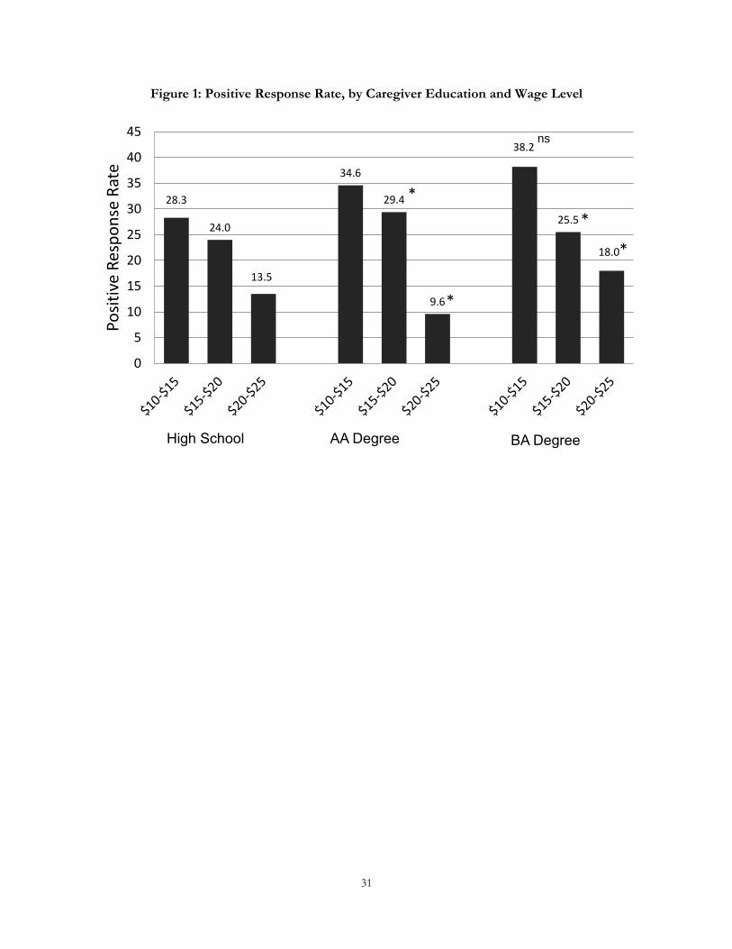
31

Figure 1: Positive Response Rate, by Caregiver Education and Wage Level

28.3

24.0

13.5

34.6

29.4

9.6

38.2

25.5

18.0

0

5

10

15

20

25

30

35

40

45P

osi

tive

Res

po

nse

Rat

e

*

ns

*

*

*

High School AA Degree BA Degree

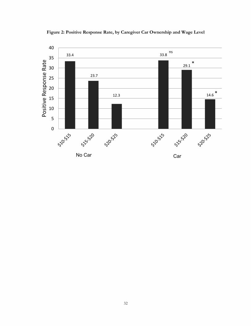
32

Figure 2: Positive Response Rate, by Caregiver Car Ownership and Wage Level

33.4

23.7

12.3

33.8

29.1

14.6

0

5

10

15

20

25

30

35

40P

osi

tive

Res

po

nse

Rat

ens

*

No Car Car

*

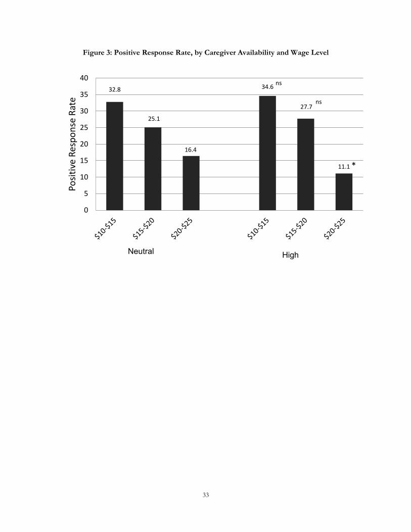
33

Figure 3: Positive Response Rate, by Caregiver Availability and Wage Level

32.8

25.1

16.4

34.6

27.7

11.1

0

5

10

15

20

25

30

35

40P

osi

tive

Res

po

nse

Rat

ens

ns

*

Neutral High

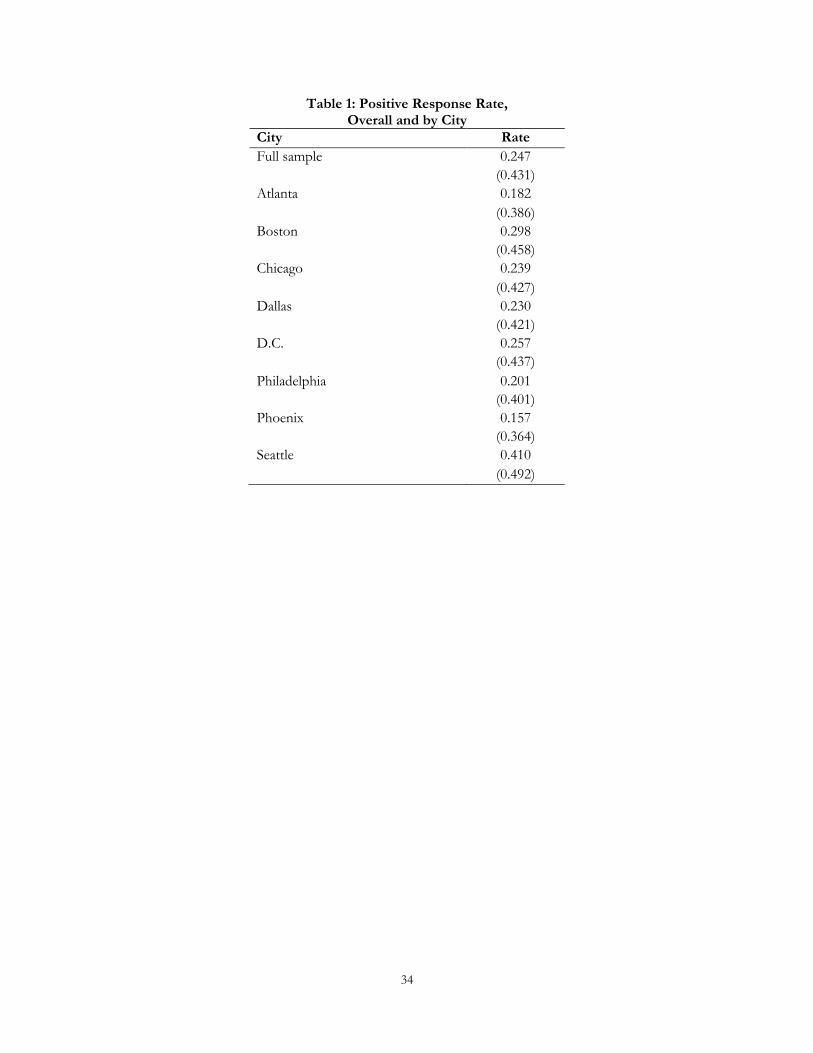
34

Table 1: Positive Response Rate, Overall and by City

City Rate

Full sample 0.247

(0.431)

Atlanta 0.182

(0.386)

Boston 0.298

(0.458)

Chicago 0.239

(0.427)

Dallas 0.230

(0.421)

D.C. 0.257

(0.437)

Philadelphia 0.201

(0.401)

Phoenix 0.157

(0.364)

Seattle 0.410

(0.492)

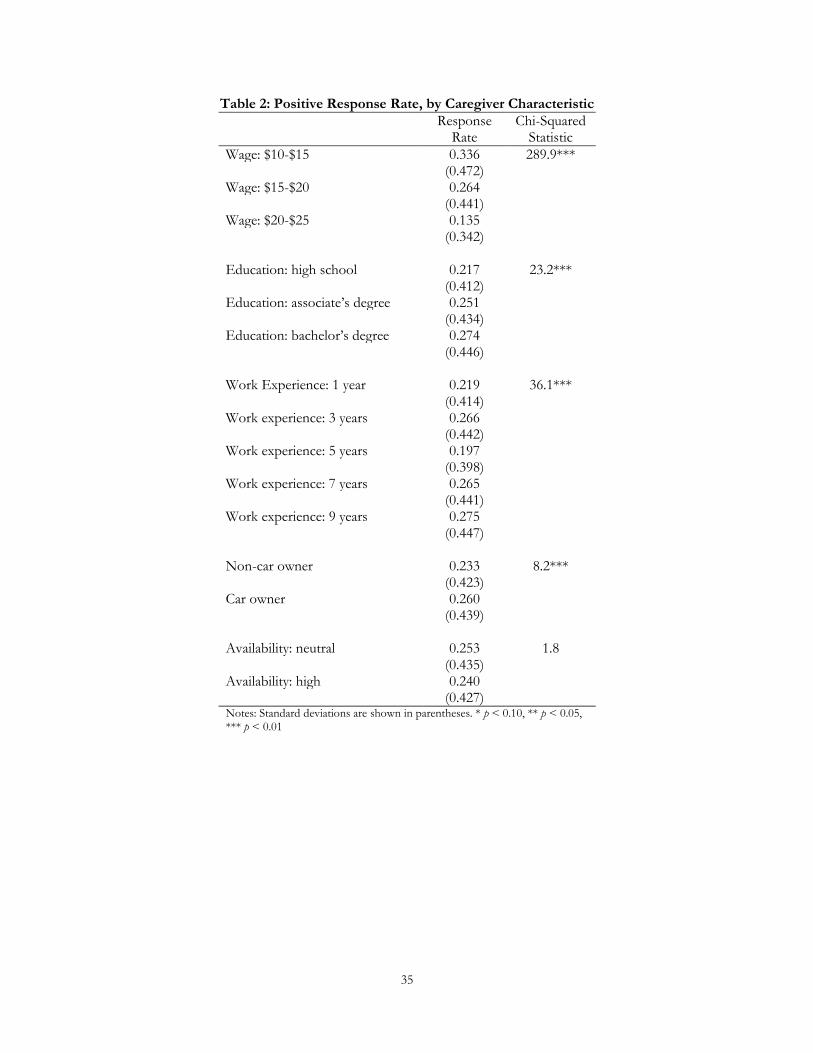
35

Table 2: Positive Response Rate, by Caregiver Characteristic

Response Rate

Chi-Squared Statistic

Wage: $10-$15 0.336 289.9*** (0.472) Wage: $15-$20 0.264 (0.441) Wage: $20-$25 0.135 (0.342) Education: high school 0.217 23.2*** (0.412) Education: associate’s degree 0.251 (0.434) Education: bachelor’s degree 0.274 (0.446) Work Experience: 1 year 0.219 36.1*** (0.414) Work experience: 3 years 0.266 (0.442) Work experience: 5 years 0.197 (0.398) Work experience: 7 years 0.265 (0.441) Work experience: 9 years 0.275 (0.447) Non-car owner 0.233 8.2*** (0.423) Car owner 0.260 (0.439) Availability: neutral 0.253 1.8 (0.435) Availability: high 0.240 (0.427) Notes: Standard deviations are shown in parentheses. * p < 0.10, ** p < 0.05, *** p < 0.01

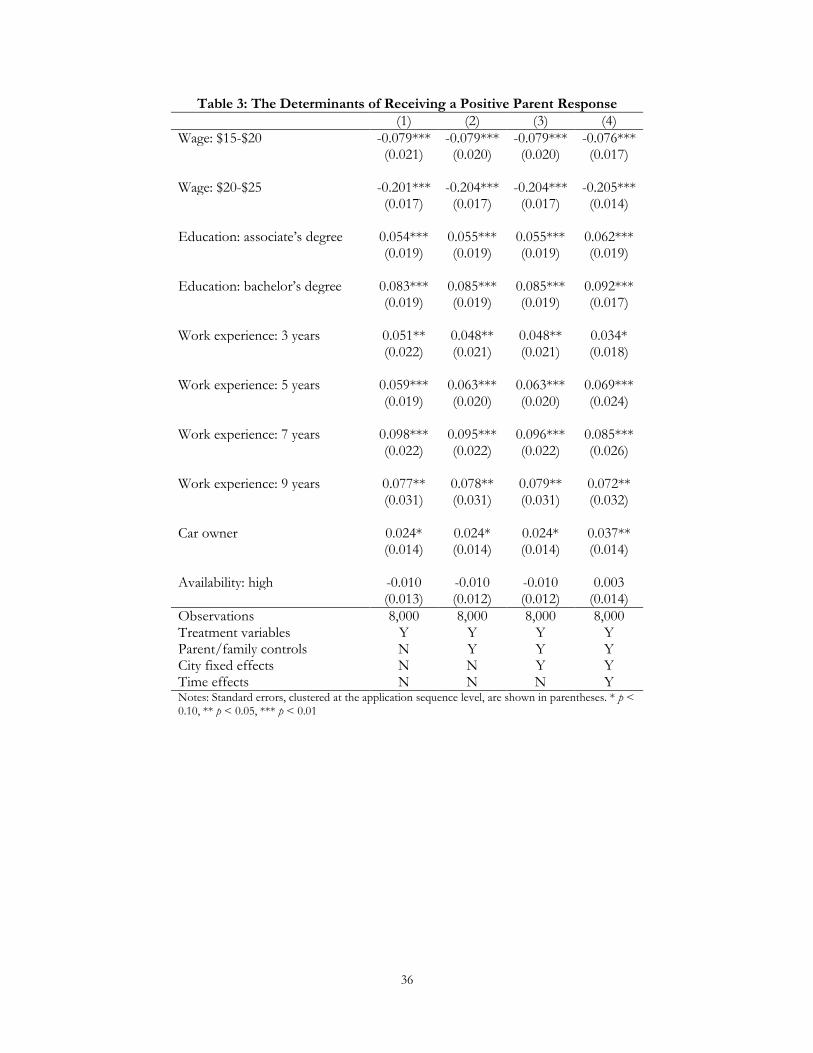
36

Table 3: The Determinants of Receiving a Positive Parent Response

(1) (2) (3) (4)

Wage: $15-$20 -0.079*** -0.079*** -0.079*** -0.076*** (0.021) (0.020) (0.020) (0.017) Wage: $20-$25 -0.201*** -0.204*** -0.204*** -0.205*** (0.017) (0.017) (0.017) (0.014) Education: associate’s degree 0.054*** 0.055*** 0.055*** 0.062*** (0.019) (0.019) (0.019) (0.019) Education: bachelor’s degree 0.083*** 0.085*** 0.085*** 0.092*** (0.019) (0.019) (0.019) (0.017) Work experience: 3 years 0.051** 0.048** 0.048** 0.034* (0.022) (0.021) (0.021) (0.018) Work experience: 5 years 0.059*** 0.063*** 0.063*** 0.069*** (0.019) (0.020) (0.020) (0.024) Work experience: 7 years 0.098*** 0.095*** 0.096*** 0.085*** (0.022) (0.022) (0.022) (0.026) Work experience: 9 years 0.077** 0.078** 0.079** 0.072** (0.031) (0.031) (0.031) (0.032) Car owner 0.024* 0.024* 0.024* 0.037** (0.014) (0.014) (0.014) (0.014) Availability: high -0.010 -0.010 -0.010 0.003 (0.013) (0.012) (0.012) (0.014)

Observations 8,000 8,000 8,000 8,000 Treatment variables Y Y Y Y Parent/family controls N Y Y Y City fixed effects N N Y Y Time effects N N N Y Notes: Standard errors, clustered at the application sequence level, are shown in parentheses. * p < 0.10, ** p < 0.05, *** p < 0.01

37

Table 4: Heterogeneity by the Age of the Youngest Child in the Family

(1) (2) (3) (4) 0-6

Months 6 Months-

3 Years 4-6

Years 7+

Years

Wage: $15-$20 -0.121*** -0.106*** -0.017 -0.003 (0.019) (0.025) (0.028) (0.036) Wage: $20-$25 -0.209*** -0.213*** -0.226*** -0.183*** (0.020) (0.026) (0.029) (0.035) Education: associate’s degree 0.035* 0.061*** 0.061** 0.114*** (0.020) (0.020) (0.028) (0.038) Education: bachelor’s degree 0.035 0.101*** 0.127*** 0.122*** (0.022) (0.029) (0.038) (0.036) Work experience: 3 years -0.000 0.049** 0.039 0.048 (0.015) (0.024) (0.036) (0.031) Work experience: 5 years 0.040 0.072* 0.050 0.120*** (0.028) (0.039) (0.044) (0.042) Work experience: 7 years 0.046** 0.102*** 0.043 0.143*** (0.021) (0.036) (0.042) (0.047) Work experience: 9 years 0.011 0.069 0.117* 0.148** (0.030) (0.049) (0.059) (0.062) Car owner 0.026 0.034* 0.079*** 0.021 (0.016) (0.018) (0.029) (0.031) Availability: high 0.017 0.001 0.001 -0.021 (0.016) (0.019) (0.021) (0.030)

Observations 2,153 2,885 1,409 1,473 Notes: Standard errors, clustered at the application sequence level, are shown in parentheses. * p < 0.10, ** p < 0.05, *** p < 0.01

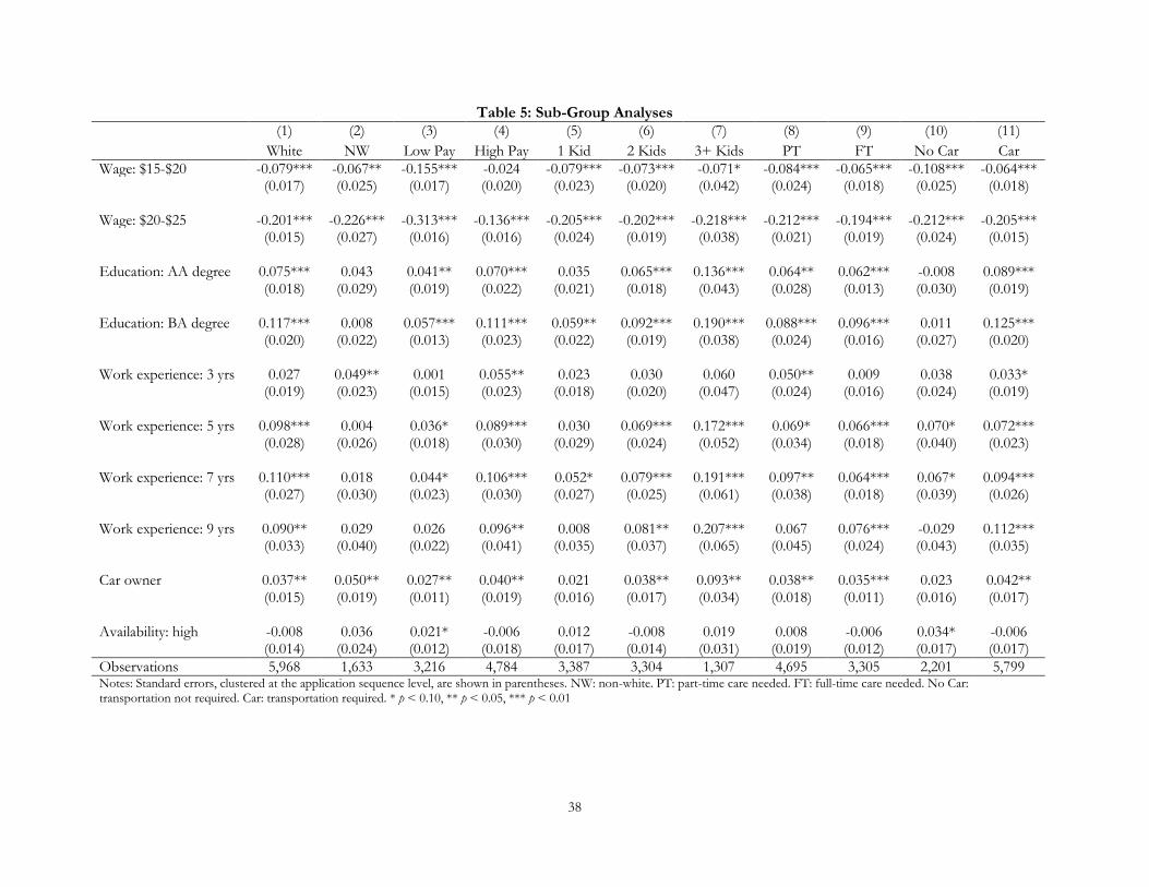
38

Table 5: Sub-Group Analyses (1) (2) (3) (4) (5) (6) (7) (8) (9) (10) (11)

White NW Low Pay High Pay 1 Kid 2 Kids 3+ Kids PT FT No Car Car

Wage: $15-$20 -0.079*** -0.067** -0.155*** -0.024 -0.079*** -0.073*** -0.071* -0.084*** -0.065*** -0.108*** -0.064*** (0.017) (0.025) (0.017) (0.020) (0.023) (0.020) (0.042) (0.024) (0.018) (0.025) (0.018) Wage: $20-$25 -0.201*** -0.226*** -0.313*** -0.136*** -0.205*** -0.202*** -0.218*** -0.212*** -0.194*** -0.212*** -0.205*** (0.015) (0.027) (0.016) (0.016) (0.024) (0.019) (0.038) (0.021) (0.019) (0.024) (0.015) Education: AA degree 0.075*** 0.043 0.041** 0.070*** 0.035 0.065*** 0.136*** 0.064** 0.062*** -0.008 0.089*** (0.018) (0.029) (0.019) (0.022) (0.021) (0.018) (0.043) (0.028) (0.013) (0.030) (0.019) Education: BA degree 0.117*** 0.008 0.057*** 0.111*** 0.059** 0.092*** 0.190*** 0.088*** 0.096*** 0.011 0.125*** (0.020) (0.022) (0.013) (0.023) (0.022) (0.019) (0.038) (0.024) (0.016) (0.027) (0.020) Work experience: 3 yrs 0.027 0.049** 0.001 0.055** 0.023 0.030 0.060 0.050** 0.009 0.038 0.033* (0.019) (0.023) (0.015) (0.023) (0.018) (0.020) (0.047) (0.024) (0.016) (0.024) (0.019) Work experience: 5 yrs 0.098*** 0.004 0.036* 0.089*** 0.030 0.069*** 0.172*** 0.069* 0.066*** 0.070* 0.072*** (0.028) (0.026) (0.018) (0.030) (0.029) (0.024) (0.052) (0.034) (0.018) (0.040) (0.023) Work experience: 7 yrs 0.110*** 0.018 0.044* 0.106*** 0.052* 0.079*** 0.191*** 0.097** 0.064*** 0.067* 0.094*** (0.027) (0.030) (0.023) (0.030) (0.027) (0.025) (0.061) (0.038) (0.018) (0.039) (0.026) Work experience: 9 yrs 0.090** 0.029 0.026 0.096** 0.008 0.081** 0.207*** 0.067 0.076*** -0.029 0.112*** (0.033) (0.040) (0.022) (0.041) (0.035) (0.037) (0.065) (0.045) (0.024) (0.043) (0.035) Car owner 0.037** 0.050** 0.027** 0.040** 0.021 0.038** 0.093** 0.038** 0.035*** 0.023 0.042** (0.015) (0.019) (0.011) (0.019) (0.016) (0.017) (0.034) (0.018) (0.011) (0.016) (0.017) Availability: high -0.008 0.036 0.021* -0.006 0.012 -0.008 0.019 0.008 -0.006 0.034* -0.006 (0.014) (0.024) (0.012) (0.018) (0.017) (0.014) (0.031) (0.019) (0.012) (0.017) (0.017)

Observations 5,968 1,633 3,216 4,784 3,387 3,304 1,307 4,695 3,305 2,201 5,799 Notes: Standard errors, clustered at the application sequence level, are shown in parentheses. NW: non-white. PT: part-time care needed. FT: full-time care needed. No Car: transportation not required. Car: transportation required. * p < 0.10, ** p < 0.05, *** p < 0.01

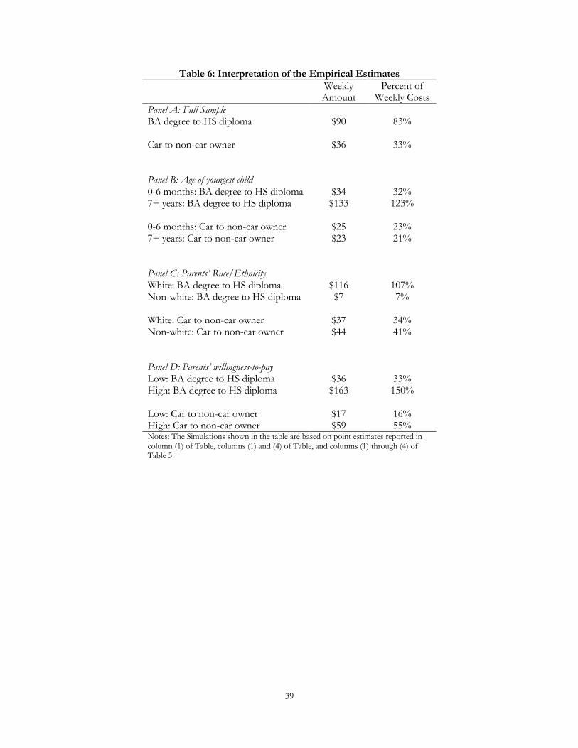
39

Table 6: Interpretation of the Empirical Estimates

Weekly Amount

Percent of Weekly Costs

Panel A: Full Sample BA degree to HS diploma $90 83% Car to non-car owner $36 33% Panel B: Age of youngest child 0-6 months: BA degree to HS diploma $34 32% 7+ years: BA degree to HS diploma $133 123% 0-6 months: Car to non-car owner $25 23% 7+ years: Car to non-car owner $23 21% Panel C: Parents’ Race/Ethnicity White: BA degree to HS diploma $116 107% Non-white: BA degree to HS diploma $7 7% White: Car to non-car owner $37 34% Non-white: Car to non-car owner $44 41% Panel D: Parents’ willingness-to-pay Low: BA degree to HS diploma $36 33% High: BA degree to HS diploma $163 150% Low: Car to non-car owner $17 16% High: Car to non-car owner $59 55% Notes: The Simulations shown in the table are based on point estimates reported in column (1) of Table, columns (1) and (4) of Table, and columns (1) through (4) of Table 5.

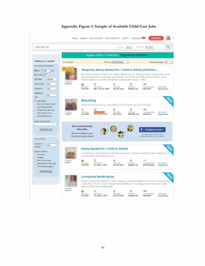
40

Appendix Figure 1: Sample of Available Child Care Jobs

41

Appendix Figure 2: Sample Parent Job Posting

42

Appendix Figure 3: Sample Caregiver Profile

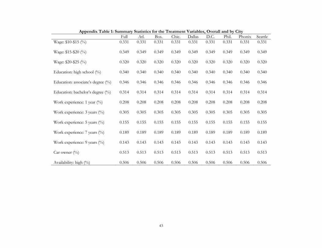
43

Appendix Table 1: Summary Statistics for the Treatment Variables, Overall and by City

Full Atl. Bos. Chic. Dallas D.C. Phil. Phonix Seattle

Wage: $10-$15 (%) 0.331 0.331 0.331 0.331 0.331 0.331 0.331 0.331 0.331 Wage: $15-$20 (%) 0.349 0.349 0.349 0.349 0.349 0.349 0.349 0.349 0.349 Wage: $20-$25 (%) 0.320 0.320 0.320 0.320 0.320 0.320 0.320 0.320 0.320 Education: high school (%) 0.340 0.340 0.340 0.340 0.340 0.340 0.340 0.340 0.340 Education: associate’s degree (%) 0.346 0.346 0.346 0.346 0.346 0.346 0.346 0.346 0.346 Education: bachelor’s degree (%) 0.314 0.314 0.314 0.314 0.314 0.314 0.314 0.314 0.314 Work experience: 1 year (%) 0.208 0.208 0.208 0.208 0.208 0.208 0.208 0.208 0.208 Work experience: 3 years (%) 0.305 0.305 0.305 0.305 0.305 0.305 0.305 0.305 0.305 Work experience: 5 years (%) 0.155 0.155 0.155 0.155 0.155 0.155 0.155 0.155 0.155 Work experience: 7 years (%) 0.189 0.189 0.189 0.189 0.189 0.189 0.189 0.189 0.189 Work experience: 9 years (%) 0.143 0.143 0.143 0.143 0.143 0.143 0.143 0.143 0.143 Car owner (%) 0.513 0.513 0.513 0.513 0.513 0.513 0.513 0.513 0.513 Availability: high (%) 0.506 0.506 0.506 0.506 0.506 0.506 0.506 0.506 0.506

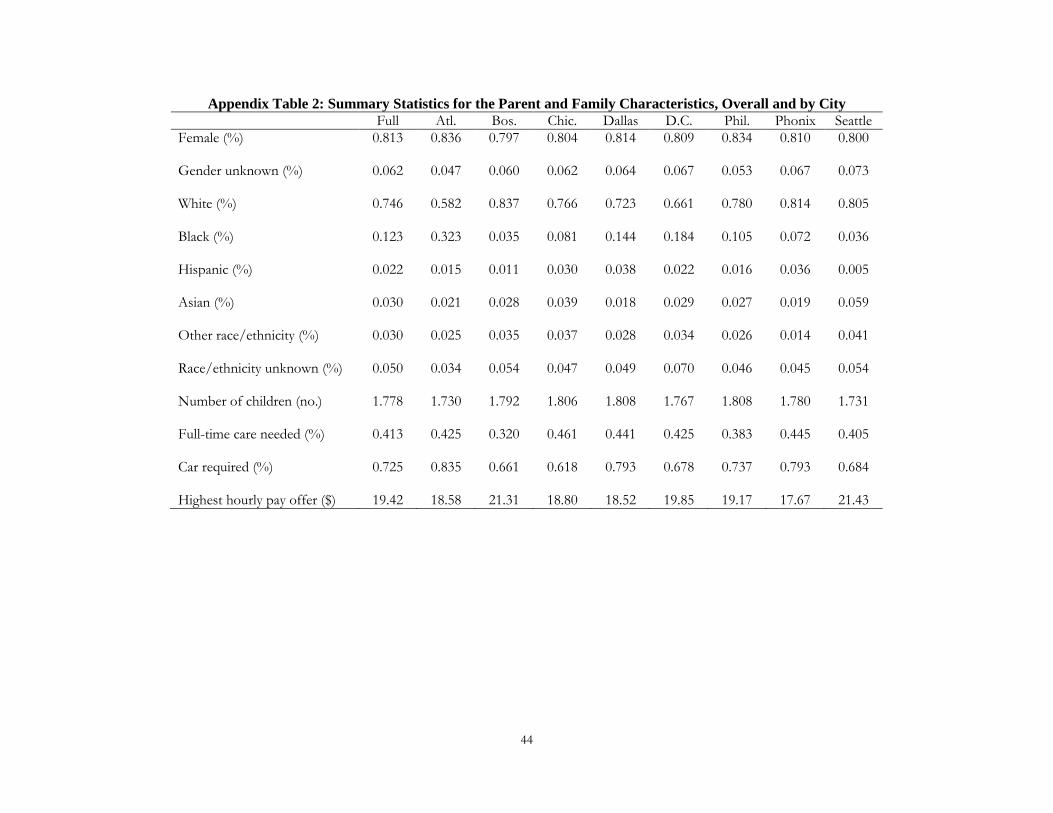
44

Appendix Table 2: Summary Statistics for the Parent and Family Characteristics, Overall and by City

Full Atl. Bos. Chic. Dallas D.C. Phil. Phonix Seattle

Female (%) 0.813 0.836 0.797 0.804 0.814 0.809 0.834 0.810 0.800 Gender unknown (%) 0.062 0.047 0.060 0.062 0.064 0.067 0.053 0.067 0.073 White (%) 0.746 0.582 0.837 0.766 0.723 0.661 0.780 0.814 0.805 Black (%) 0.123 0.323 0.035 0.081 0.144 0.184 0.105 0.072 0.036 Hispanic (%) 0.022 0.015 0.011 0.030 0.038 0.022 0.016 0.036 0.005 Asian (%) 0.030 0.021 0.028 0.039 0.018 0.029 0.027 0.019 0.059 Other race/ethnicity (%) 0.030 0.025 0.035 0.037 0.028 0.034 0.026 0.014 0.041 Race/ethnicity unknown (%) 0.050 0.034 0.054 0.047 0.049 0.070 0.046 0.045 0.054 Number of children (no.) 1.778 1.730 1.792 1.806 1.808 1.767 1.808 1.780 1.731 Full-time care needed (%) 0.413 0.425 0.320 0.461 0.441 0.425 0.383 0.445 0.405 Car required (%) 0.725 0.835 0.661 0.618 0.793 0.678 0.737 0.793 0.684 Highest hourly pay offer ($) 19.42 18.58 21.31 18.80 18.52 19.85 19.17 17.67 21.43

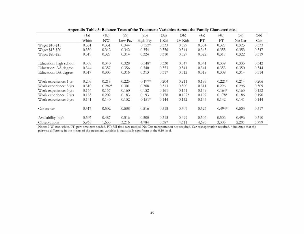
45

Appendix Table 3: Balance Tests of the Treatment Variables Across the Family Characteristics

(1a) (1b) (2a) (2b) (3a) (3b) (4a) (4b) (5a) (5b)

White NW Low Pay High Pay 1 Kid 2+ Kids PT FT No Car Car

Wage: $10-$15 0.331 0.331 0.344 0.322* 0.333 0.329 0.334 0.327 0.325 0.333 Wage: $15-$20 0.350 0.342 0.342 0.354 0.356 0.344 0.345 0.355 0.353 0.347 Wage: $20-$25 0.319 0.327 0.314 0.324 0.310 0.327 0.322 0.317 0.322 0.319 Education: high school 0.339 0.340 0.328 0.348* 0.330 0.347 0.341 0.339 0.335 0.342 Education: AA degree 0.344 0.357 0.356 0.340 0.353 0.341 0.341 0.353 0.350 0.344 Education: BA degree 0.317 0.303 0.316 0.313 0.317 0.312 0.318 0.308 0.314 0.314 Work experience: 1 yr 0.209 0.218 0.225 0.197* 0.204 0.211 0.199 0.221* 0.214 0.206 Work experience: 3 yrs 0.310 0.282* 0.301 0.308 0.313 0.300 0.311 0.296 0.296 0.309 Work experience: 5 yrs 0.154 0.157 0.160 0.152 0.161 0.151 0.149 0.164* 0.163 0.152 Work experience: 7 yrs 0.185 0.202 0.183 0.193 0.178 0.197* 0.197 0.178* 0.186 0.190 Work experience: 9 yrs 0.141 0.140 0.132 0.151* 0.144 0.142 0.144 0.142 0.141 0.144 Car owner 0.517 0.502 0.508 0.516 0.518 0.509 0.527 0.494* 0.503 0.517 Availability: high 0.507 0.487 0.516 0.500 0.515 0.499 0.506 0.506 0.496 0.510

Observations 5,968 1,633 3,216 4,784 3,387 4,611 4,695 3,305 2,201 5,799 Notes: NW: non-white. PT: part-time care needed. FT: full-time care needed. No Car: transportation not required. Car: transportation required. * indicates that the pairwise difference in the means of the treatment variables is statistically significant at the 0.10 level.

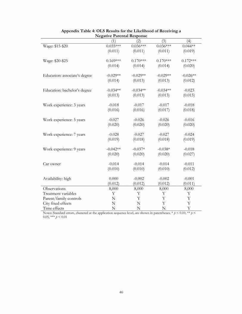
46

Appendix Table 4: OLS Results for the Likelihood of Receiving a Negative Parental Response

(1) (2) (3) (4)

Wage: $15-$20 0.035*** 0.036*** 0.036*** 0.044** (0.011) (0.011) (0.011) (0.019) Wage: $20-$25 0.169*** 0.170*** 0.170*** 0.172*** (0.014) (0.014) (0.014) (0.020) Education: associate’s degree -0.029** -0.029** -0.029** -0.026** (0.014) (0.013) (0.013) (0.012) Education: bachelor’s degree -0.034** -0.034** -0.034** -0.023 (0.013) (0.013) (0.013) (0.015) Work experience: 3 years -0.018 -0.017 -0.017 -0.018 (0.016) (0.016) (0.017) (0.018) Work experience: 5 years -0.027 -0.026 -0.026 -0.016 (0.020) (0.020) (0.020) (0.020) Work experience: 7 years -0.028 -0.027 -0.027 -0.024 (0.019) (0.018) (0.018) (0.019) Work experience: 9 years -0.042** -0.037* -0.038* -0.018 (0.020) (0.020) (0.020) (0.027) Car owner -0.014 -0.014 -0.014 -0.011 (0.010) (0.010) (0.010) (0.012) Availability: high 0.000 -0.002 -0.002 -0.001 (0.012) (0.012) (0.012) (0.011)

Observations 8,000 8,000 8,000 8,000 Treatment variables Y Y Y Y Parent/family controls N Y Y Y City fixed effects N N Y Y Time effects N N N Y Notes: Standard errors, clustered at the application sequence level, are shown in parentheses. * p < 0.10, ** p < 0.05, *** p < 0.01

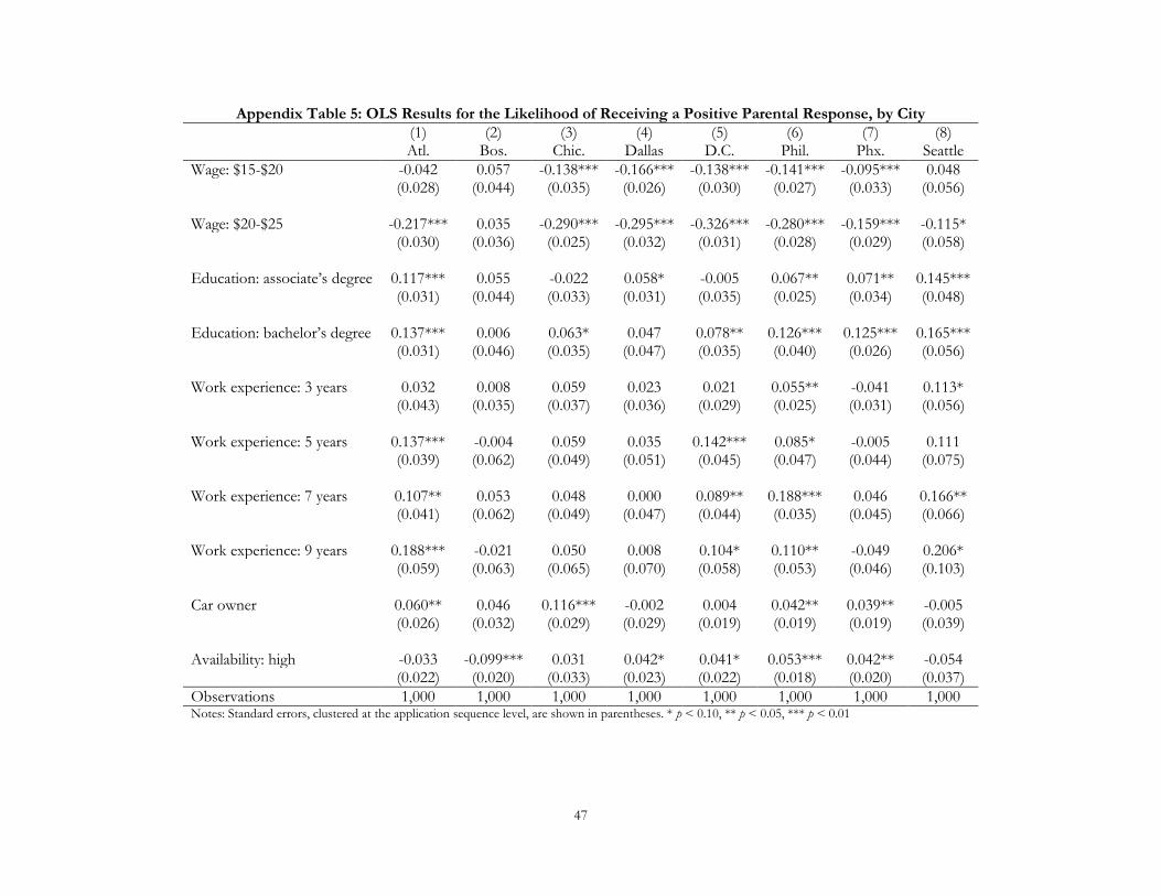
47

Appendix Table 5: OLS Results for the Likelihood of Receiving a Positive Parental Response, by City

(1) (2) (3) (4) (5) (6) (7) (8) Atl. Bos. Chic. Dallas D.C. Phil. Phx. Seattle

Wage: $15-$20 -0.042 0.057 -0.138*** -0.166*** -0.138*** -0.141*** -0.095*** 0.048 (0.028) (0.044) (0.035) (0.026) (0.030) (0.027) (0.033) (0.056) Wage: $20-$25 -0.217*** 0.035 -0.290*** -0.295*** -0.326*** -0.280*** -0.159*** -0.115* (0.030) (0.036) (0.025) (0.032) (0.031) (0.028) (0.029) (0.058) Education: associate’s degree 0.117*** 0.055 -0.022 0.058* -0.005 0.067** 0.071** 0.145*** (0.031) (0.044) (0.033) (0.031) (0.035) (0.025) (0.034) (0.048) Education: bachelor’s degree 0.137*** 0.006 0.063* 0.047 0.078** 0.126*** 0.125*** 0.165*** (0.031) (0.046) (0.035) (0.047) (0.035) (0.040) (0.026) (0.056) Work experience: 3 years 0.032 0.008 0.059 0.023 0.021 0.055** -0.041 0.113* (0.043) (0.035) (0.037) (0.036) (0.029) (0.025) (0.031) (0.056) Work experience: 5 years 0.137*** -0.004 0.059 0.035 0.142*** 0.085* -0.005 0.111 (0.039) (0.062) (0.049) (0.051) (0.045) (0.047) (0.044) (0.075) Work experience: 7 years 0.107** 0.053 0.048 0.000 0.089** 0.188*** 0.046 0.166** (0.041) (0.062) (0.049) (0.047) (0.044) (0.035) (0.045) (0.066) Work experience: 9 years 0.188*** -0.021 0.050 0.008 0.104* 0.110** -0.049 0.206* (0.059) (0.063) (0.065) (0.070) (0.058) (0.053) (0.046) (0.103) Car owner 0.060** 0.046 0.116*** -0.002 0.004 0.042** 0.039** -0.005 (0.026) (0.032) (0.029) (0.029) (0.019) (0.019) (0.019) (0.039) Availability: high -0.033 -0.099*** 0.031 0.042* 0.041* 0.053*** 0.042** -0.054 (0.022) (0.020) (0.033) (0.023) (0.022) (0.018) (0.020) (0.037)

Observations 1,000 1,000 1,000 1,000 1,000 1,000 1,000 1,000 Notes: Standard errors, clustered at the application sequence level, are shown in parentheses. * p < 0.10, ** p < 0.05, *** p < 0.01