dimensions of the welfare state and economic performance ... · dimensions of the welfare state and...

COYUNTURA ECONÓMICA Y DOTACIÓN SOCIAL EN LA ECUACIÓN INTERGENERACIONAL DE BECKER TOMES. UNA ESTIMACIÓN PARA ESPAÑA 2002-2013

CAPÍTULO 5: CAPITAL HUMANO Y CRECIMIENTO ECONÓMICO 811

Dimensions of the welfare state and economic performance: a comparative

analysis

JOÃO A. S. ANDRADEA

ADELAIDE P. S. DUARTEB

MARTA C. N. SIMÕESC

a,b,cGEMF – Grupo de Estudos Monetários e Financeiros; Faculty of Economics; University of Coimbra; Portugal

[email protected]

In recent years the desirability of an extensive Welfare State has been increasingly questioned on the grounds that economies with less social intervention by the Government are more competitive and productive. But even if countries do not increase public expenditure, changing the composition of the Welfare State might foster growth by rescaling their intervention in domains that are productivity enhancing. Education and health are the most striking examples given their role as sources of human capital, a fundamental ingredient in many growth models. It is thus important to empirically assess the impact of public expenditures on education and health on educational attainment and health status indicators, and real income. We do this for three groups of countries: a group of high income OECD economies, the EU before the enlargement and the EU enlargement group. We identitfy long-run

relationships across the main variables using the DOLS estimator corrected for cross-sectional dependence and we estimate short-run relationships that include an ECM term from the associated long-run equation by applying Fixed-Effects and Pooled Mean Group estimators for the period 1960-2012. The results of the estimation of the long-run equilibrium relationships point to a positive, direct or indirect, influence of (public) education expenditures and (public, private or total) health expenditures on output for the three groups of countries. Causality relationships exhibit mixed results concerning policy variables, within and between country groups, with the results for the high-income OECD (non EU) group supporting the use of social policy variables to foster economic growth. Keywords: education, health, public expenditures, economic growth, OECD

INVESTIGACIONES DE ECONOMÍA DE LA EDUCACIÓN NÚMERO 10

812 CHAPTER 5: HUMAN CAPITAL AND ECONOMIC GROWTH

1. INTRODUCTION

There is a long-standing debate in the economic literature on the influence of the Welfare

State on economic performance and controversies still remain on the sign of this relationship.

For some authors, according to Hoareau-Sautieres and Rascle (2005), public social spending is

an impediment to a good economic performance because: it discourages savings and

investment; its funding uses scarce resources and introduces distortions in economic activity; it

hampers job creation and increases unemployment, and it is more inefficient than the market

in covering certain social responsibilities. Arguments in the opposite direction suggest that the

Welfare State cannot be understood only in terms of the economic costs that it entails since

the services it offers have important benefits, namely in terms of output and productivity

growth as well as generating positive externalities. An often cited author in defense of the

Welfare State, Peter Lindert1, argues that the Welfare State has, among others, allowed

countries to achieve higher levels of equality without leading to a slowdown in output growth,

a situation which the author designates as the "free lunch puzzle" (Lindert (2002; 2004);

Lindert (2006a)). According to the same author, the adverse effects of state intervention in

economic performance result from other forms of action such as the design of the legal

framework and the regulation of certain markets (Lindert (2006b)).

From an economic growth perspective, two important dimensions of the Welfare State are

public expenditures on education and health, to the extent that they lead to the accumulation

of human capital, which plays a central role in growth models, both exogenous and

endogenous. A healthier and more educated population/workforce corresponds in principle to

a higher availability of human capital in the economy, thereby improving productivity and

increasing in this way output (Mankiw et al. (1992); Lucas (1988)). In advanced economies it

increases the respective innovation capability (Romer (1990); Jones (1995); Jones (2005)) and

in those that are below the technological frontier it allows the diffusion and transmission of

knowledge in order to process new information and implement successful technologies

developed by the leaders (Nelson and Phelps (1966); Abramovitz (1986); Benhabib and Spiegel

(1994); Benhabib and Spiegel (2005)). Investment in education and health can thus generate

substantial returns over time, not just at the individual level, but especially for the economy as

a whole, and the Welfare State can play a crucial role in this dynamic process.

The main objective of this work is to contribute to the debate on the economic impact of the

Welfare State by focusing on two of its dimensions, the provision (directly or indirectly) of

education and health services, and assessing their importance for long-run macroeconomic

performance. For this purpose, we apply panel data methodologies that allow us to identify

long-run equilibrium relationships and also test for causality. We first test for the presence of

panel unit roots and in this way check the resilience of health and education variables,

correcting for the presence of cross-sectional correlation. Next we estimate growth

regressions to identify long-run equilibrium relationships. Finally, based on the previous results

we analyze causality between education and health variables and output, as well as between

1 See e.g. http://ideas.repec.org/f/c/pli466.html.

http://ideas.repec.org/f/c/pli466.html

DIMENSIONS OF THE WELFARE STATE AND ECONOMIC PERFORMANCE: A COMPARATIVE ANALYSIS


the former and different social indicators that influence the welfare levels of the population.

We consider three samples of countries from the European Union (EU) and high-income non-

EU OECD countries listed in the World Development Indicators database of the World Bank

over the period (maximum) 1960-2012. All the countries included are classified as developed

high-income countries by the World Bank. In any case, the three groups present sufficient

variation in the respective income levels to make it possible to accommodate the hypothesis

that the impact of education and health expenditures on economic growth varies according to

income levels.

The remainder of this work is structured as follows. In section 2 we describe the data used and

the methodology applied. Section 3 presents and discusses the results. Finally, section 4

outlines the main conclusions.

2. DATA AND METHODOLOGY

The main aim of this paper is to empirically investigate the link between health and education

expenditures, output and welfare indicators. Our variables of interest thus refer to the

different dimensions under analysis. Annual data from 1960 to 2012, when possible, were

obtained from the World Development Indicators (WDI) database of the World Bank. Our

database is an unbalanced panel. Table 1 describes the variables in the database, where

column (1) contains our notations, column (2) contains the WDI notation and column (3) the

definitions of the variables.

Table 1. Variables in the database

(1) (2) (3)

x NE.EXP.GNFS.ZS Exports of goods and services (% of GDP)

gfc NE.GDI.FTOT.ZS Gross fixed capital formation (% of GDP)

py NY.GDP.DEFL.ZS GDP defluator (base year varies by country)

yrpc NY.GDP.PCAP.PP.KD GDP per capita, PPP (constant 2005 international $)

es SE.SEC.ENRR School enrollment, secondary (% gross)

et SE.TER.ENRR School enrollment, tertiary (% gross)

eep SE.XPD.TOTL.GD.ZS Public spending on education, total (% of GDP)

hepr SH.XPD.PRIV.ZS Health expenditure, private (% of GDP)

hep SH.XPD.PUBL.ZS Health expenditure, public (% of GDP)

mi SP.DYN.IMRT.IN Mortality rate, infant (per 1,000 live births)

leb SP.DYN.LE00.IN Life expectancy at birth, total (years)

Note: (1) our notation; (2) WDI notation and (3) WDI variable description.



We consider three groups of countries (Table 2) that we identify as Eu_1, Eu_2 and OECD_w.

The first group (Eu_1) corresponds to the European Union before enlargement to the East in

2004 (except Luxembourg) and is composed of fourteen countries; the second group (Eu_2)

contains the thirteen new member states that joined the EU after 2004; and the third group

(OECD_w) the wealthiest OECD non-EU countries in a total of ten countries.

Table 2. Groups of Countries

Eu_1 Austria, Belgium, Germany, Denmark, Spain, Finland, France, United Kingdom, Greece, Ireland, Italy, Netherlands, Portugal, Sweden

Eu_2 Bulgaria, Cyprus, Czech R., Estonia, Croatia, Hungary, Lithuania, Latvia, Malta, Poland, Romania, Slovenia, Slovak R.

OECD_w Australia, Canada, Switzerland, Israel, Iceland, Japan, S. Korea, Norway, New Zealand, U.S.A.

Table 3 contains some descriptive statistics for the different variables in our database across

the three different groups of countries. From the inspection of Table 3 it is possible to see that

the variables present different characteristics across the three groups in terms of the

coefficient of variation and the median. For exports (x), the group Eu_2 records a higher

median value than the other two groups. Median investment (gfc) and median inflation (dpy)

are not very different across groups. Inflation stability is more obvious for Eu_1 relative to the

two other groups. In terms of GDP per capita, Eu_1 is the most homogeneous and Eu_2 has a

median value that corresponds to half of the value for the other two groups. In what concerns

education and health variables (es, et, eep, hep and hepr), Eu_2 presents lower median values.

However, infant mortality rate (mi) and life expectancy (leb) values are relatively more stable

for the Eu_2 group, while the median values are clearly worse than for the other two groups.

Table 3. Descriptive statistics for the three groups

Eu_1 Eu_2 OECD_w

Variable VC Med VC Med VC Med

x 0.506 28.03 0.302 49.46 0.411 28.42

gfc 0.163 21.58 0.198 23.00 0.201 23.60

dpy 0.700 0.038 2.480 0.041 2.360 0.043

yrpc 0.148 25428 0.348 12948 0.305 27294

es 0.135 98.97 0.068 90.78 0.135 95.65

et 0.202 34.74 0.431 23.76 0.470 40.02

eep 0.238 5.09 0.236 4.41 0.220 5.35

hep 0.191 6.78 0.237 4.78 0.248 6.24

hepr 0.303 2.13 0.470 1.88 0.672 2.49

mi 0.803 8.80 0.537 14.55 0.558 8.10

leb 0.047 74.98 0.039 70.90 0.058 75.86

Notes: VC- coefficient of variation; Med – median



The empirical strategy we apply aims at implementing a coherent methodology to overcome

the drawbacks of some of the previous empirical literature that uses panel causality. In

particular, we want to analyse long-run equilibrium relations between our variables,

identifying differences across groups, and use estimators and models suitable for non-

stationary variables, while at the same time controlling for problems of cross-sectional

dependence.

Our empirical strategy is implemented in two stages. The first stage includes two steps, (A) and

(B), and the second the stage is composed of step (C). In the first stage, we start by studying

the stationarity characteristics of the variables taking into account the phenomena of cross-

sectional dependence (step A). We next estimate long-run equilibrium relations by applying

non-stationary methods to regressions that include both state and policy variables (step B).

We estimate a benchmark model that considers only state variables. Next we compare the

results of estimating models with state and policy variables added to the results of the former

model. These models are retained if the associated level of information is higher than the one

for the benchmark model. Finally, in the second stage of our empirical strategy (step C) we

identify the 'error correction mechanism' (ECM) from the corresponding long-run relations and

define the dynamic short run equations that allow us to test for the existence of weak-

exogeneity. If we cannot reject the null hypothesis of weak-exogeneity this means that the

dependent variable of the short-run model is not caused by the other variables in the long-run

relationship.

In what follows we describe in more detail the tests applied and the models estimated. In step

(A) of the first stage of our empirical strategy, we apply unity root tests considering the

presence of cross-sectional dependence. We use an ADF test specific for panel data with a null

hypothesis (H0) corresponding to the presence of a unit root in all series, against the

alternative that at least one of the series is stationary. This test is built as a combination of the

significance levels of the ADF tests, Choi (2001), based on the inverse of the Normal

distribution. For N fixed individuals and T observations sufficiently numerous (T ), if H0

applies:

1

1

1( ) (0,1)

N d

i

i

Z p NN

In this formulation the test assumes cross-sectional independence. Costantini and Lupi (2013)

propose to correct for cross-sectional dependence based on Hartung (1999) and Demetrescu et

al. (2006) and a suitable formula for test computation Demetrescu et al. (2006) is used:

1

1

1 2

( )

Z

2ˆ ˆ1 * 0.2 1 * 1

1

N

i

iH

p

N NN

where ˆ * is a convergent estimator of , and 1( )ip denotes the common correlation:



2

1 1 1 1

1 1

ˆ (1 1 ( ) ( )N N

i i

i i

N p N p

We apply this test without or with trend. We also apply the covariate augmented Dickey-Fuller

test (CADF) proposed in Costantini and Lupi (2013) and based on Hansen (1995) and Hanck

(2013). Originally it tests for the presence of a unit root in panel data with or without sectional

correlation, Pesaran (2004). This test performs better than the ordinary ADF test. Following

Hansen (1995), the power of the CADF test is improved when a stationary variable is included

in the augmented equation. The new equation is thus, at the individual level:

1 1( ) ( )t t t ta L Y Y b L x e

where a(L) and b(L) are polynomial lags, x is the added covariate and the errors ( e ) have the

usual properties. Costantini and Lupi (2013) suggest using as a stationary variable the average

of the first difference, applied to all individuals, or the first difference of the first principal

component of the variable. This change allows to increase the power of the test when

compared to the usual averages of ADF tests. The correction of cross-sectional correlation

assumes the significance level of the Pesaran (2004) test is less than the typical value, so that

10% is considered an acceptable choice. We use a test based on Hartung (1999) and

Demetrescu et al. (2006) that automatically corrects for sectional correlation with the

threshold set at 10% and considering as covariate the first difference of the variable under

analysis. We will also perform the above mentioned tests with a constant and with a constant

and a trend. These four tests will be identified as Zh, Zh(t), pCADF and pCADF(t), respectively,

where (t) stands for the presence of a trend, Lupi (2011; 2013).

In the second step, (B), of the first stage, we begin our analysis of the long-run relations

between our variables of interest by considering an equilibrium model including state and

policy variables (1):

(1) , , , ,i t j i t l i t i tY X Z ò

where X is a (kx1) set of state variables, βj the (1xk) set of corresponding coefficients and Z and

γh a set of (lx1) and (1xl) policy variables and coefficients, respectively; i and t denote countries

and time, respectively.

We first consider what we call a benchmark equation (1) that icludes only state variables (py, x,

gfc) and where yrpc is the dependent variable. We next consider equations (2) and (3) to

investigate the joint influence of the two dimensions of human capital, - education (secondary

and tertiary levels) and health (life expectancy and infant mortality both at birth) on (yrpc).

Next we examine the influence of the social policy variables, - education expenditures and

health expenditures on yrpc. The former analysis corresponds to equation (4) and the latter to

equations ((5), (6), (7), (8), (9)), in order to assess the influence of (public, private and total)

health expenditures on (yrpc) equations. Since our main aim is to test for the influence of the

education and health expenditures variables, as social policy variables, we also estimate

equations (10), (11), (12) and (13), to test for their impact on the education levels ((es), (et))

and on the health status welfare variables ((mi), (leb)).



To robustly estimate equation (1) we have to consider the presence of cross-sectional

correlation and that the variables are integrated of order 1. To solve the first problem we

included the individual (sectional) averages of each of the variables in equation (1), aW ,

Pesaran (2006). To overcome the second problem we added lags and leads of order s of the

first difference of the independent variables, ΔW, with s=1, following Saikkonen (1991)

proposition to apply DOLS. Our estimated parameters βj and γh correspond to the expected

long-run parameters in equation (1a):

(1a) ,

*

, , ,,,i t j i t l i t i

sa

l i t m i t t

h s

Y X Z W W

ò

where W contains the sets of variables X and Z and aW contains the sets of variables W and Y.

Finally, the second stage (step C) of our empirical strategy consists in the estimation of the

dynamic short-run equations, using the results to test for weak exogeneity. We can define our

dynamic short-run equation, with , 1 ,ECM i t i tò from equation (1), as:

(2) *

, , , ,

1

( ) m

k h

i t i i t l i t i t

l

Y ECM L W

where θl(L) represents a lag polynomial of some order. We have imposed a lag polynomial of

degree one. We consider two hypotheses for the short-run dynamic behavior. According to the

first one, which we call intercept heterogeneity behavior we assume that institutional

differences and other omitted variables are important determinants of the equilibrium path.

The second hypothesis assumes that the long-run equilibrium path is even more dependent on

institutional variables so we cannot only assume intercept heterogeneity, we have to consider

heterogeneity of all the coefficients. To investigate the first hypothesis we apply the Fixed

Effects (FE) estimator and for the second one we use the Pooled Mean Group (PMG)

estimator. Since the concept of Granger (1969) causality implies that the variables are

stationary the second stage of our empirical strategy is appropriate for this analysis but we

restrict our analysis to what is sometimes named as 'long-run causality' (weak exogeneity).

3. RESULTS

The results of the unit root tests (step A) for each of the three groups of countries under

analysis can be found in Table 4. All the variables are in logs and the notation used for the first

difference of a variable K is ‘dK’. The statistics corrected for cross-sectional dependence are in

italics and correspond to the majority of cases. According to the results presented in Table 4,

for all the variables in each of the groups we cannot reject the presence of a unit root for the

variable in levels but we reject it for the variable in first differences.



Table 4. Unit Roots tests results for Eu_1, Eu_2 and OECD_w

Eu_1 Eu_2 OECD_w

Var. 1 2 3 4 5 6 7 8 9 10 11 12

x 1.05 -1.19 -0.07 -3.18 *** -2.60 *** -2.32 ** -2.75 *** -2.67 *** -2.18 ** -3.01 ** -1.14 -2.16 **

dx -6.09 *** -5.96 *** 10.19 *** -4.44 *** -5.59 *** -4.78 *** -7.40 *** -7.99 *** -7.00 *** -6.55 *** -13.09 *** -11.25 ***

gfc -0.69 -1.15 -2.36 *** -2.54 *** -0.89 -0.53 -4.24 *** -4.36 *** -2.63 *** -1.63 * -1.98 ** -1.95 **

dgfc -7.44 *** -9.98 *** -10.78 *** -8.90 *** -10.76 *** -9.30 *** -7.45 *** -2.50 *** -4.39 *** -4.10 *** -11.26 *** -9.60 ***

py -1.05 -1.36 0.94 1.80 -5.19 *** -4.81 *** -0.26 -3.34 *** -1.47 * 1.60 -2.41 *** -3.84 ***

dpy -0.33 -0.80 -1.80 ** -1.73 ** -8.35 *** -6.10 *** -4.51 -4.23 *** -3.59 *** -4.94 *** -7.37 *** -6.17 ***

yrpc -0.46 4.00 0.16 3.75 0.24 2.16 0.08 -1.29 * 0.73 -0.12 1.42 -1.36 *

dyrpc -6.35 *** -5.72 *** -1.94 ** 0.68 -1.90 ** -1.66 ** -2.53 *** -2.09 ** -2.93 *** -2.72 *** -7.90 *** -6.97 ***

es -0.80 1.19 -0.99 -1.14 -1.57 * -2.27 ** -4.36 *** -5.89 *** -0.79 -0.01 -1.45 * -0.86

des -5.01 *** -4.51 *** -7.85 *** -9.07 *** -11.34 *** -9.32 *** -8.94 *** -5.96 *** -8.85 *** -7.55 *** -6.04 *** -4.81 ***

et 1.29 0.23 2.19 -0.78 2.84 0.41 -6.82 *** -3.46 *** 0.21 0.48 4.05 0.35

det -10.70 *** -8.74 *** -8.28 *** -6.68 *** -5.78 *** -4.00 *** -3.54 *** -5.49 *** -10.35 *** -9.48 *** -6.41 *** -5.77 ***

eep -0.79 -0.27 -5.99 *** -1.06 -1.09 -1.89 ** -2.54 *** -1.52 * -0.18 -0.58 -2.82 *** -4.01 ***

deep -12.26 *** -10.71 *** -8.49 *** -6.90 *** 9.57 *** -7.60 *** -4.26 *** -3.00 *** -11.31 *** -9.84 *** -8.80 *** -8.37 ***

hepr 0.08 -0.72 1.90 -1.31 * -0.38 -1.34 * 0.77 -3.90 *** 1.04 -1.10 -0.56 -1.72 **

dhepr -2.34 *** -1.79 ** -6.51 *** -7.07 *** -3.25 *** -2.85 *** -8.40 *** --- -2.81 *** -2.27 *** -12.41 *** -4.96 ***

hep 2.08 -2.24 ** 0.75 -3.96 *** -0.98 -0.67 -1.93 ** -1.17 0.41 -1.28 0.49 -3.26 ***

dhep -2.90 ** -1.56 * -7.28 *** -6.78 *** -4.03 *** -1.56 -7.64 *** -6.19 *** -3.04 *** -2.78 *** -8.67 *** -7.36 ***

mi 1.70 0.41 1.93 -1.71 ** 5.93 0.10 1.54 -3.31 -1.46 * 3.02 -1.88 ** -0.98

dmi -1.38 * -0.69 -3.02 *** -3.06 *** -0.09 0.09 -1.47 * -1.87 ** -0.25 -0.93 -1.80 ** -1.94 **

leb 8.15 -0.08 5.04 -0.01 8.42 3.84 5.08 0.04 3.71 -2.52 *** 2.59 -1.15

dleb -18.40 *** -20.40 *** -7.57 *** -21.50 *** -14.68 *** -15.04 *** -9.94 *** --- -14.80 *** -14.24 *** 3.81 -17.90 ***

Notes: The first to fourth columns for each group contain the values of the tests Zh, Zh(t), pCADF and pCADF(t), respectively,

where (t) stands for the presence of a trend. Zh, Zh(t), pCADF and pCADF(t) have as the null hypothesis (H0) the presence of a unit

root in all the series against the alternative that at least one of the series is stationary. The stars have the usual interpretation, ***

if the null is rejected at the 1% significance level, ** for 5% and * for 10%.

The results of the estimation of the long run relations with the variables integrated of order 1

(step B) are presented in Tables 5, 6 and 7, for the groups Eu_1, Eu_2 and OECD_w,

respectively. The overall conclusions in terms of the long-run behavior are: educational

attainment and health status matter for output growth and education expenditures are an

important determinant of educational attainment levels, while health expenditures are an

important determinant of health status. The first equation that appears in the Tables 5-7 is our

benchmark equation.

For the EU_1 group (Table 5), our benchmark equation (1) with output (yrpc) as the dependent

variable considers as state variables, prices (py), exports (x) and investment (gfc). Equations 2

and 3 examine the importance of human capital for output behaviour proxied, respectively, by

secondary education attainment levels, (es), and life expectancy at birth (leb), and tertiary

education attainment levels, (et)2,3. These equations present a better level of information (BIC)

2 We have also estimated equations (2) and (3) with the welfare variable infant mortality at birth, (mi), instead of

(leb) but the coefficient was never statistically significant in any of the country groups. 3 In the case of equation (3) we started by estimating an equation with (leb). However, since the coefficient was

not statistically significant we next estimated the equation reported in Table 7 that includes only the education indicator (et), and we adopted the same procedure for equations 2 and 3 in the case of the two other country groups whenever necessary.



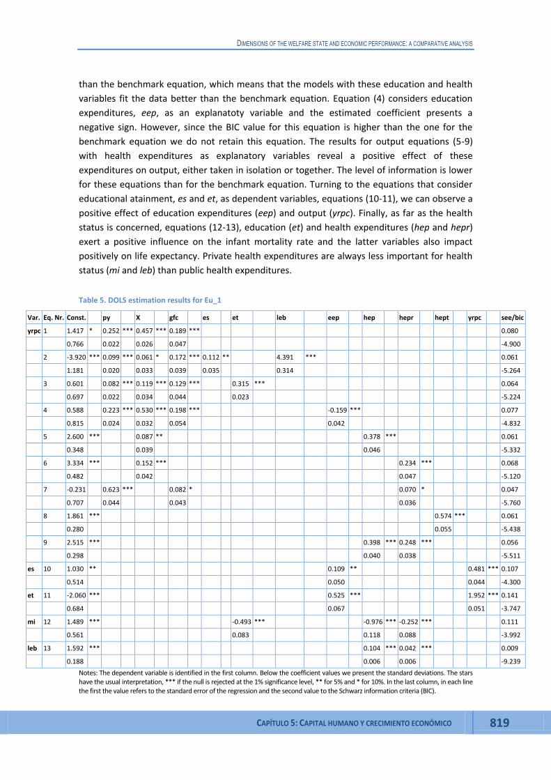
than the benchmark equation, which means that the models with these education and health

variables fit the data better than the benchmark equation. Equation (4) considers education

expenditures, eep, as an explanatoty variable and the estimated coefficient presents a

negative sign. However, since the BIC value for this equation is higher than the one for the

benchmark equation we do not retain this equation. The results for output equations (5-9)

with health expenditures as explanatory variables reveal a positive effect of these

expenditures on output, either taken in isolation or together. The level of information is lower

for these equations than for the benchmark equation. Turning to the equations that consider

educational atainment, es and et, as dependent variables, equations (10-11), we can observe a

positive effect of education expenditures (eep) and output (yrpc). Finally, as far as the health

status is concerned, equations (12-13), education (et) and health expenditures (hep and hepr)

exert a positive influence on the infant mortality rate and the latter variables also impact

positively on life expectancy. Private health expenditures are always less important for health

status (mi and leb) than public health expenditures.

Table 5. DOLS estimation results for Eu_1

Var. Eq. Nr. Const. py X gfc es et leb eep hep hepr hept yrpc see/bic

yrpc 1 1.417 * 0.252 *** 0.457 *** 0.189 *** 0.080

0.766 0.022 0.026 0.047 -4.900

2 -3.920 *** 0.099 *** 0.061 * 0.172 *** 0.112 ** 4.391 *** 0.061

1.181 0.020 0.033 0.039 0.035 0.314 -5.264

3 0.601 0.082 *** 0.119 *** 0.129 *** 0.315 *** 0.064

0.697 0.022 0.034 0.044 0.023 -5.224

4 0.588 0.223 *** 0.530 *** 0.198 *** -0.159 *** 0.077

0.815 0.024 0.032 0.054 0.042 -4.832

5 2.600 *** 0.087 ** 0.378 *** 0.061

0.348 0.039 0.046 -5.332

6 3.334 *** 0.152 *** 0.234 *** 0.068

0.482 0.042 0.047 -5.120

7 -0.231 0.623 *** 0.082 * 0.070 * 0.047

0.707 0.044 0.043 0.036 -5.760

8 1.861 *** 0.574 *** 0.061

0.280 0.055 -5.438

9 2.515 *** 0.398 *** 0.248 *** 0.056

0.298 0.040 0.038 -5.511

es 10 1.030 ** 0.109 ** 0.481 *** 0.107

0.514 0.050 0.044 -4.300

et 11 -2.060 *** 0.525 *** 1.952 *** 0.141

0.684 0.067 0.051 -3.747

mi 12 1.489 *** -0.493 *** -0.976 *** -0.252 *** 0.111

0.561 0.083 0.118 0.088 -3.992

leb 13 1.592 *** 0.104 *** 0.042 *** 0.009

0.188 0.006 0.006 -9.239

Notes: The dependent variable is identified in the first column. Below the coefficient values we present the standard deviations. The stars have the usual interpretation, *** if the null is rejected at the 1% significance level, ** for 5% and * for 10%. In the last column, in each line the first the value refers to the standard error of the regression and the second value to the Schwarz information criteria (BIC).



As far as the second group of countries, Eu_2, is concerned (Table 6), the benchmark equation

is the same as that for Eu_1 and again all the equations that consider the education and health

variables on the right hand side present a better level of information relative to the benchmark

equation. For this group, education expenditures (eep) present an estimated coefficient with a

positive sign and the BIC value for the respective equation is better than for the benchmark

equation. Contrary to the results for EU_1, equation (3) includes the health status indicator

(leb), statistically significant at the 1% level. The results for the equations that consider

educational attainment or the health status as dependent variable are similar to those for the

EU_1 group. The exception is the equation with the infant mortality rate as dependent

variable, equation (11), where the results do not support the existence of a relationship with

educational attainment (et), and the opposite applies to output.

Table 6. DOLS estimation results for Eu_2

Var. Eq. Nr. Const. py x gfc es et leb eep hep hepr hept yrpc see/bic

yrpc 1 0.942 0.043 *** 0.410 *** 0.162 ** 0.185

0.598 0.010 0.072 0.080 -3.101

2 -3.333 0.034 *** 0.128 *** 0.223 *** 0.904 *** 5.222 *** 0.108

3.394 0.006 0.048 0.057 0.120 0.437 -4.003

3 -2.377 0.112 *** 0.333 *** 0.252 *** 2.519 *** 0.096

2.443 0.040 0.043 0.019 0.502 -4.328

4 1.444 *** 0.042 *** 0.454 *** 0.311 *** 0.510 *** 0.169

0.596 0.010 0.076 0.090 0.073 -3.151

5 -0.876 ** 0.431 *** 0.792 *** 0.157

0.392 0.070 0.142 -3.425

6 -0.685 ** 0.298 *** 0.416 *** 0.141

0.349 0.068 0.049 -3.638

7 -0.772 ** 1.251 *** 0.154

0.384 0.127 -3.581

8 -0.704 ** 0.611 *** 0.425 *** 0.139

0.343 0.126 0.047 -3.665

es 9 1.110 ** 0.107 *** 0.171 *** 0.067

0.504 0.027 0.023 -5.195

et 10 0.374 0.896 *** 1.899 *** 0.314

0.805 0.127 0.107 -2.103

mi 11 7.674 *** -0.344 ** -0.111 * -0.895 *** 0.154

0.939 0.150 0.064 0.088 -3.354

leb 12 -0.859 *** 0.029 ** 0.010 ** 0.052 *** 0.012

0.252 0.014 0.005 0.007 -8.503

See Notes to Table 5.

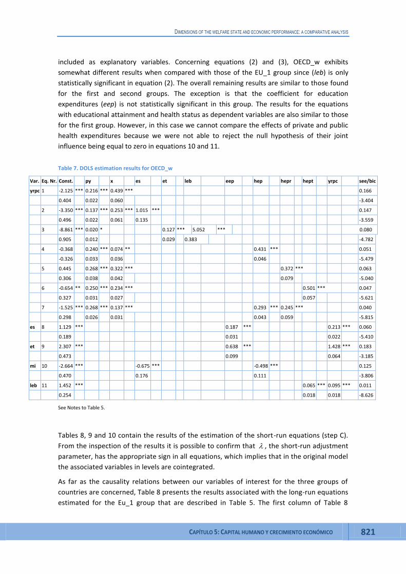
The results for the OECD_w group (Table 7) point to a benchmark equation for output with

only prices (py) and exports (x) as state variables, leaving out investment that was statistically

significant for the other two groups. For the equations with output as dependent variable

there is an information gain when educational attainment and health status variables are



included as explanatory variables. Concerning equations (2) and (3), OECD_w exhibits

somewhat different results when compared with those of the EU_1 group since (leb) is only

statistically significant in equation (2). The overall remaining results are similar to those found

for the first and second groups. The exception is that the coefficient for education

expenditures (eep) is not statistically significant in this group. The results for the equations

with educational attainment and health status as dependent variables are also similar to those

for the first group. However, in this case we cannot compare the effects of private and public

health expenditures because we were not able to reject the null hypothesis of their joint

influence being equal to zero in equations 10 and 11.

Table 7. DOLS estimation results for OECD_w

Var. Eq. Nr. Const. py x es et leb eep hep hepr hept yrpc see/bic

yrpc 1 -2.125 *** 0.216 *** 0.439 *** 0.166

0.404 0.022 0.060 -3.404

2 -3.350 *** 0.137 *** 0.253 *** 1.015 *** 0.147

0.496 0.022 0.061 0.135 -3.559

3 -8.861 *** 0.020 * 0.127 *** 5.052 *** 0.080

0.905 0.012 0.029 0.383 -4.782

4 -0.368 0.240 *** 0.074 ** 0.431 *** 0.051

-0.326 0.033 0.036 0.046 -5.479

5 0.445 0.268 *** 0.322 *** 0.372 *** 0.063

0.306 0.038 0.042 0.079 -5.040

6 -0.654 ** 0.250 *** 0.234 *** 0.501 *** 0.047

0.327 0.031 0.027 0.057 -5.621

7 -1.525 *** 0.268 *** 0.137 *** 0.293 *** 0.245 *** 0.040

0.298 0.026 0.031 0.043 0.059 -5.815

es 8 1.129 *** 0.187 *** 0.213 *** 0.060

0.189 0.031 0.022 -5.410

et 9 2.307 *** 0.638 *** 1.428 *** 0.183

0.473 0.099 0.064 -3.185

mi 10 -2.664 *** -0.675 *** -0.498 *** 0.125

0.470 0.176 0.111 -3.806

leb 11 1.452 *** 0.065 *** 0.095 *** 0.011

0.254 0.018 0.018 -8.626

See Notes to Table 5.

Tables 8, 9 and 10 contain the results of the estimation of the short-run equations (step C).

From the inspection of the results it is possible to confirm that , the short-run adjustment

parameter, has the appropriate sign in all equations, which implies that in the original model

the associated variables in levels are cointegrated.

As far as the causality relations between our variables of interest for the three groups of

countries are concerned, Table 8 presents the results associated with the long-run equations

estimated for the Eu_1 group that are described in Table 5. The first column of Table 8



contains the number of the long-run equation that appears after the benchmark equation in

Table 5. dY refers to the equation of the first difference of the dependent variable in the

respective long-run equation and dX1, dX2 and dX3 to the equations for the associated

policy variables and, eventually, for yrpc, if retained as an independent variable, according to

the ordering of the variables of the corresponding equation in Table 5. For instance, if we

consider equation (2) the null hypothesis that the coefficient of the equation with dY as

dependent variable is zero is rejected at the 1% significance level when using either of the

two estimation methods (FE and PMG). Additionally, the null hypothesis that the coefficient

associated with the short-run equation for dX1(=es) is zero is not rejected when using

both estimation methods. However, the null hypothesis that the coefficient associated

with the short-run equation for dX2(=leb) is zero is rejected when using both estimation

methods. These results imply that in the cointegration relation defined between the

variables in equation (2), (es) is weakly exogenous, while (leb) and (yrpc) are endogenous. In

the former case the disequilibrium values do not influence the short run behavior of (es) and

so the causality goes from (es) to (yrpc). In the latter case, on the contrary, (lep) is caused by

(yrpc). In our causality analysis we take 5% as the limit significance level for rejection of the

null hypothesis that the estimated adjustment coefficient is zero. If rejection of the null

hypothesis only applies at the 10% significance level we ignore whether the variable can be

considered as weakly exogenous or endogenous. A similar interpretation can be made of the

results presented in Tables 9 and 10 for Eu_2 and OECD_w, respectively, in what concerns

causality analysis. We will analyze the causality results according to the order of

presentation of the results in Tables 5-7.

The results concerning Eu_1 (Table 8) and OECD_w (Table 10) imply that (es) is weakly

exogenous in equation 2 with both the FE and the PMG estimators. However, for Eu_2 (Table

9) it is (et) that is weakly exogenous in equation 3 with both FE and PMG. These results

indicate that for the two samples with higher per capita income levels (OECD_w and Eu_1),

the educational attainment variable (es) is a policy variable since it is not caused by (yrpc),

which might be the consequence of the compulsory nature of this level of education in these

two groups of countries. In what concerns Eu_2, the fact that (es) is not weakly exogenous,

but (et) is, might be explained by the fact that these countries had a highly educated

workforce under the socialist regime and, after the end of the regime, they recorded,

simultaneously, a huge decrease in per capita income and a considerable increase in income

inequality during the transition period towards a market economy. In what concerns the

health status indicator (leb) and using comparable human capital proxies, (leb) is weakly

exogenous for Eu_2 and OECD_w, no matter the estimation method used. But if we compare

Eu_1 with Eu_2 using equation 2 we observe opposite results: ( leb) is endogenous for Eu_1

and weakly exogenous for Eu_2.



Table 8. ECM Coefficient for Results on Table 5 (Eu_1)

Fixed Effects Pooled Mean Group

Eq. dY dX1 dX2 dX3 dY dX1 dX2 dX3

2 -0.093 *** -0.029 0.008*** -0.287 *** 0.065 0.022**

0.019 0.043 0.002 0.058 0.114 0.010

3 -0.113 *** 0.027 0.310 *** -0.116 *

0.017 0.042 0.033 0.066

5 -0.167 *** 0.298 *** -0.223 *** 0.456 ***

0.023 0.052 0.032 0.077

6 -0.152 *** 0.115 -0.238 *** 0.176 *

0.019 0.072 0.038 0.093

7 -0.128 *** 0.178 -0.194 *** 0.488 **

0.036 0.112 0.067 0.239

8 -0.157 *** 0.290 *** -0.182 *** 0.448 ***

0.024 0.041 0.031 0.056

9 -0.171 *** 0.330 *** 0.234 *** -0.203 *** 0.521 *** 0.303 ***

0.024 0.053 0.084 0.032 0.073 0.116

10 -0.098 *** 0.025 ** -0.007 -0.114 *** 0.204 *** -0.489 ***

0.023 0.010 0.031 0.031 0.063 0.171

11 -0.053 *** 0.040 *** 0.023 -0.125 *** -0.030 -0.007

0.019 0.013 0.025 0.018 0.179 0.028

12 -0.047 *** -0.115 *** -0.127 *** -0.169 ** -0.053 *** -0.148 *** -0.371 *** -0.238 ***

0.014 0.037 0.047 0.074 0.001 0.054 0.001 0.001

13 -0.006 ** 0.009 0.233 *** -0.020 *** 0.251 *** 0.422 ***

0.003 0.045 0.068 0.001 0.001 0.001

Notes: The first column presents the number of the long-run equation that appears after the benchmark equation in the

respective table. dY refers to the equation of the first difference of the dependent variable and dX1, dX2 and dX3 to the equations

of the policy variables and, eventually, yrpc, if retained as an independent variable, following the ordering of the variables of the

associated equation in Table 5. Below the coefficient values we present the standard deviations. The stars have the usual

interpretation, *** if the null is rejected at the 1% significance level, ** for 5% and * for 10%.

Table 9. ECM Coefficient for Results in Table 6 (EU_2)



2 -0.144 *** 0.018 0.002 -0.097 ** 0.070 ** 0.009

0.023 0.019 0.003 0.049 0.035 0.007

3 -0.140 *** -0.062 -0.001 -0.208 *** 0.130 0.006

0.026 0.053 0.003 0.064 0.112 0.009

4 -0.062 *** 0.508 *** -0.099 *** 0.452 ***

0.014 0.079 0.026 0.065

5 -0.088 *** 0.138 *** -0.104 *** 0.221 ***

0.017 0.032 0.022 0.046

6 -0.105 *** 0.066 -0.112 ** 0.314 ***

0.020 0.065 0.042 0.098

7 -0.087 *** 0.133 *** -0.091 *** 0.226 ***





0.017 0.025 0.020 0.036

8 -0.096 *** 0.159 *** 0.064 -0.110 *** 0.254 *** 0.158 *

0.019 0.035 0.061 0.225 0.056 0.087

9 -0.159 *** 0.876 *** 0.003 -0.210 *** 0.687 0.161

0.033 0.244 0.048 0.076 0.600 0.103

10 -0.009 0.252 *** 0.041 *** 0.008 0.247 0.074 ***

0.016 0.049 0.010 0.026 0.166 0.020

11 -0.001 -0.059 -0.036 0.003 -0.057 *** -0.078 0.116 -0.053

0.009 0.058 0.095 0.026 0.015 0.116 0.167 0.049

12 -0.121 *** 0.950 -0.676 0.391 -0.107 ** 2.306 ** 0.347 0.417

0.040 0621 1.031 0.303 0.051 0.934 1.464 0.356

Note: The first column has the number of the long-run equation after the baseline equation. dY refers to the equation of the first

difference of the dependent variable and dX1, dX2 and dX3 to the equations of the policy variables and eventually yrpc, if

independent variable, following the order of the variables of the associated equation in Table 6. See also Note to Table 8.

Table 10. ECM Coefficient for Results on Table 7 (OECD_w)


Eq. dY dX1 dX2 dY dX1 dX2

2 -0.054 *** -0.005 -0.094 *** 0.006

0.009 0.009 0.016 0.020

3 -0.090 *** 0.011 0.008* -0.147 *** 0.257 ** 0.016***

0.018 0.046 0.005 0.030 0.119 0.005

4 -0.191 *** 0.229 ** -0.161 ** 0.379 **

0.040 0.089 0.067 0.163

5 -0.127 *** 0.091 -0.150 *** -0.061

0.031 0.081 0.038 0.169

6 -0.164 *** 0.106 -0.165 *** 0.116

0.039 0.076 0.049 0.160

7 -0.125 *** 0.026 0.069 -0.146 *** -0.182 -0.131

0.031 0.072 0.080 0.042 0.163 0.169

8 -0.096 *** 0.029 0.048 * -0.115 *** -0.050 0.067 *

0.023 0.087 . 0.025 0.031 0.095 0.035

9 -0.057 *** 0.041 0.013 -0.114 *** 0.016 0.023 *

0.021 0.029 0.008 0.028 0.041 0.013

10 -0.034 *** 0.020 0.004 -0.084 *** -0.062 * -0.230 ***

0.009 0.017 0.034 0.022 0.032 0.087

11 -0.387 *** 0.294 0.045 -0.298 *** 1.457 0.535

0.068 0.428 0.238 0.068 1.013 0.570

Note: The first column has the number of the long-run equation after the baseline equation. dY refers to the equation of the first

difference of the dependent variable and dX1, dX2 and dX3 to the equations of the policy variables and eventually yrpc, if

independent variable, following the order of the variables of the associated equation in Table 7. See also Note to Table 8.



If we turn now to the results that allow us to identify the causality relations between (es) and

(eep) and (et) and (eep) in order to ascertain whether (eep) might be classified as a policy

variable, we find mixed results that are sensitive to the estimators used. The only exception is

the OECD_w group for which public spending in education is weakly exogenous for both

relations described above and with both estimators that is (eep) is not caused by (es) nor by

(et). In what concerns the other two groups, public spending in education is only weakly

exogenous for Eu_2 using the PMG estimator in the framework of equation (9).

As for the causality relations between (yrpc) and health expenditures, the results are those

associated with equations (5) to (9) for Eu_1 (Tables 5 and 8), equations (5) to (8) for Eu_2

(Tables 6 and 9) and equations (4) to (7) for OECD_w (Tables 7 and 10). For this last group and

for both estimators, public, private and total health expenditures (as a % of GDP) are weakly

exogenous, meaning that these variables are not caused in the long-run by real GDP per capita.

As far as the other two country groups are concerned, we observe opposite results – the

variables (hep), (hept), (hepr) and (hep) are not weakly exogenous implying that in the long-run

they are caused by real GDP per capita.

When we inspect the causality relations between health status variables and health

expenditures, we observe that for the equations where (leb) is the dependent variable (hep) is

weakly exogenous only with the FE estimator, in the case of Eu_1, whereas (hepr) and (yrpc)

are weakly exogenous for Eu_2 and both estimators. Finally, for the OECD_w group (hept) and

(yrpc) are weakly exogenous for both estimators. As for the results concerning the equations

where (mi) is the dependent variable, we observe mixed results: (hep) and (hepr) are

endogenous for Eu_1 and exogenous for Eu_2 and (et) is endogenous for Eu_1, while (es) is

sensitive to the estimators in the OECD_w group.

4. CONCLUSIONS

In this paper we empirically assess the impact of public expenditures on education and health

on real income and educational attainment and health status indicators. We do this for three

groups of countries: a group of high income OECD non-EU economies, the EU before the

enlargement and the EU enlargement group.

The results concerning the long-run equations reveal a positive, direct or indirect, influence of

(public) education expenditures and of (public, private or total) health expenditures on output

and hence support the argument that the Welfare State is growth enhancing for the three

groups of countries under analysis. These findings are not in line with the evidence found in

other previous cross-country studies that point to a negative impact in developed countries,

which can be explained by the different methodology used that we claim is more robust. We

found also that educational attainment levels matter for output growth, although the relevant

level in the long-run differs across country groups. We found that for our three groups the

influence of health expenditures on output is similar – public, private and total health

expenditures have a positive influence on output but public health expenditures exert a

stronger influence. When we consider the health status welfare as dependent variable both

public and private health expenditures influence the infant mortality rate and life exceptancy



at birth in both EU country groups. As for the high-income non- EU OECD group, the influence

only applies to total health expenditures. Public health expenditures again exhert a stronger

influence on the health status welfare variables.

Our results reveal causality relationships that are sensitive to the estimators used and the

country group under analysis. If a variable is weakly exogenous this implies means that,

although there is a long-run equilibrium relationship between the variables, in the short-run

the weakly exogenous variable causes the other variables, but the opposite does not apply.

According to this definition, weakly exogenous social policy variables are in reality

discretionary policy variables that might be used as policy instruments in the short-run in order

to positively influence, directly or indirectly, long-run equilibrium output. From our results we

concluded that the high-income non-EU OECD group exhibits discretionary social policy

variables that might be used to foster long-run equilibrium output and health status welfare,

but this is not the case for the other two groups. In the older EU member states social policy

variables are endogenous and the results for the enlargement group lies are mixed. In

particular, health expenditures cause health status welfare but cause output only indirectly.

This means that for the EU member states, education and health policies react to

desequilibrim towards the long-run equilibrium path, being endogenously determined with

output, which undermines their use as growth enhancing policies. The associated policy

recommendation is that these social policies should also become discretionary policies in the

EU since the policy variables beneath them also exert a positive and quantitatively important

influence on long-run output and welfare. However, most EU member statest have been

severely hit by the global financial crisis that started in 2007-2008, evolving into an economic

crisis in 2009, and to a sovereign debt crisis in several Economic and Monetary Union (EMU)

countries. Many EU countries are thus constrained by fiscal austerity measures and the

prospects for economic recovery and growth in the EU are dim. Under these circumstances

this policy recommendation faces severe impediments but it should be taken seriously by EU

governments’ since it does not necessarily involve increasing expenditures, it might be done by

changing the composition of public expenditure in general, and social expenditure in

particular.

REFERENCES

Abramovitz, M. 1986. Catching up, forging ahead and falling behind. Journal of Economic History 46 (2): 385-406.

Benhabib, J. and M. Spiegel. 1994. The role of human capital in economic development: Evidence from aggregate cross-country data. Journal of Monetary Economics 34 (2): 143-73.

Benhabib, J. and M. Spiegel. 2005. Human capital and technology diffusion. In Handbook of economic growth, eds Aghion, P and Durlauf, S, Chapter 13, 935-66 Amsterdam: North

Choi, I. 2001. Unit root tests for panel data. Journal of International Money and Finance 20 (2): 249-72.

Costantini, M. and C. Lupi. 2013. A simple panel-cadf test for unit roots. Oxford Bulletin of Economics and Statistics 75 (2): 276-96.

Demetrescu, M., U. Hassler and A.-I. Tarcolea. 2006. Combining significance of correlated statistics with application to panel data. Oxford Bulletin of Economics and Statistics 68 (5): 647-63.



Granger, C.W.J. 1969. Investigating causal relations by econometric models and cross- spectral methods. Econometrica 37 (3): 424-38.

Hanck, C. 2013. An intersection test for panel unit roots. Econometric Reviews 32 (2): 183-203.

Hansen, B.E. 1995. Rethinking the univariate approach to unit root testing: Using covariates to increase power. Econometric Theory 11 (05): 1148-71.

Hartung, J. 1999. A note on combining dependent tests of significance. Biometrical Journal 41 (7): 849-55.

Hoareau-Sautieres, E. and M. Rascle. 2005. Social welfare systems and economic performance the opposing arguments. «Economic performance and social welfare», European Social Insurance Platform (ESIP) CONFERENCE, PARIS, 9th December 2005.

Jones, C.I. 1995. R&d-based models of economic growth. Journal of Political Economy 103 (41): 759-84.

Jones, C.I. 2005. Growth and ideas. In Handbook of economic growth, eds Aghion, P and Durlauf, S, Chapter 16. Amsterdam: North-Holland.

Lindert, P. 2002. Why the welfare state looks like a free lunch. mimeo, Harvard University.

Lindert, P. 2004. Growing public: Social spending and economic growth since the eighteenth century. 2 vols. Cambridge: Cambridge University Press.

Lindert, P. 2006a. The welfare state is the wrong target: A reply to bergh. Econ Journal Watch 3 (2): 236-50.

Lindert, P. 2006b. What has happened to the inefficient welfare state? Address to the National Academy of Social Insurance.

Lucas, R. 1988. On the mechanics of economic development. Journal of Monetary Economics 22: 3-42.

Lupi, C. 2011. Panel-cadf testing with r: Panel unit root tests made easy. Economics & Statistics Discussion Paper, University of Molise, Dept. SEGeS 063.

Lupi, C. 2013. 'Cadftest', package for r. http://cran.r-project.org February, 15.

Mankiw, N.G., D. Romer and D. Weil. 1992. A contribution to the empirics of economic growth. Quarterly Journal of Economics 107 (2): 407-37.

Nelson, R.R. and E.S. Phelps. 1966. Investment in humans, technological diffusion and economic growth. American Economic Review 56 (1/2): 69-75.

Pesaran, M.H. 2004. General diagnostic tests for cross section dependence in panels. Cambridge Working Papers in Economics 0435.

Pesaran, M.H. 2006. Estimation and inference in large heterogenous panels with multifactor error structure. Econometrica 74: 967-1012.

Romer, P. 1990. Human capital and growth: Theory and evidence. Carnegie-Rochester Conference Series on Public Policy 32: 251-86.

Saikkonen, P. 1991. Asymptotically efficient estimation of cointegrating regressions. Econometric Theory 58 (1-21).

http://cran.r-project.org/

dimensions of the welfare state and economic performance ... · dimensions of the welfare state and...

Documents