dipartimento di scienze e innovazione tecnologica ... · colin maclaurin building, riccarton,...

arX

iv:1

710.

1146

7v3

[he

p-th

] 3

0 Ja

n 20

18

EMPG–17–16

Nonassociative differential geometry

and gravity with non-geometric fluxes

Paolo Aschieri1, Marija Dimitrijevic Ciric2 and Richard J. Szabo3

1 Dipartimento di Scienze e Innovazione Tecnologica, Universita del Piemonte Orientale,

Viale T. Michel 11, 15121 Alessandria, Italy

and INFN, Sezione di Torino, via P. Giuria 1, 10125 Torino, Italy

and Arnold-Regge Center, via P. Giuria 1, 10125, Torino, Italy

Email: [email protected]

2 Faculty of Physics, University of Belgrade

Studentski trg 12, 11000 Beograd, Serbia


3 Department of Mathematics, Heriot-Watt University

Colin Maclaurin Building, Riccarton, Edinburgh EH14 4AS, U.K.

and Maxwell Institute for Mathematical Sciences, Edinburgh, U.K.

and The Higgs Centre for Theoretical Physics, Edinburgh, U.K.


Abstract

We systematically develop the metric aspects of nonassociative differential geometry tailoredto the parabolic phase space model of constant locally non-geometric closed string vacua,and use it to construct preliminary steps towards a nonassociative theory of gravity onspacetime. We obtain explicit expressions for the torsion, curvature, Ricci tensor and Levi-Civita connection in nonassociative Riemannian geometry on phase space, and write downEinstein field equations. We apply this formalism to construct R-flux corrections to theRicci tensor on spacetime, and comment on the potential implications of these structures innon-geometric string theory and double field theory.

http://arxiv.org/abs/1710.11467v3

Contents

1 Introduction 3

2 Algebraic structure of non-geometric flux deformations 5

2.1 R-flux induced cochain twist and quasi-Hopf algebra . . . . . . . . . . . . . . . . 5

2.2 Associator identities . . . . . . . . . . . . . . . . . . . . . . . . . . . . . . . . . . 7

2.3 Double field theory formulation . . . . . . . . . . . . . . . . . . . . . . . . . . . . 8

3 Nonassociative deformation of tensor calculus 10

3.1 Principles of twist deformation . . . . . . . . . . . . . . . . . . . . . . . . . . . . 10

3.2 Functions . . . . . . . . . . . . . . . . . . . . . . . . . . . . . . . . . . . . . . . . 11

3.3 Forms . . . . . . . . . . . . . . . . . . . . . . . . . . . . . . . . . . . . . . . . . . 11

3.4 Tensors . . . . . . . . . . . . . . . . . . . . . . . . . . . . . . . . . . . . . . . . . 13

3.5 Duality . . . . . . . . . . . . . . . . . . . . . . . . . . . . . . . . . . . . . . . . . 14

3.6 Module homomorphisms . . . . . . . . . . . . . . . . . . . . . . . . . . . . . . . . 15

3.7 Quantum Lie algebra of diffeomorphisms . . . . . . . . . . . . . . . . . . . . . . . 19

4 Nonassociative differential geometry 20

4.1 Connections . . . . . . . . . . . . . . . . . . . . . . . . . . . . . . . . . . . . . . . 20

4.2 Dual connections . . . . . . . . . . . . . . . . . . . . . . . . . . . . . . . . . . . . 22

4.3 Connections on tensor products . . . . . . . . . . . . . . . . . . . . . . . . . . . . 23

4.4 Torsion . . . . . . . . . . . . . . . . . . . . . . . . . . . . . . . . . . . . . . . . . 24

4.5 Curvature . . . . . . . . . . . . . . . . . . . . . . . . . . . . . . . . . . . . . . . . 26

4.6 Ricci tensor . . . . . . . . . . . . . . . . . . . . . . . . . . . . . . . . . . . . . . . 31

5 Nonassociative Riemannian geometry and gravity 33

5.1 Metric and torsion-free connection conditions . . . . . . . . . . . . . . . . . . . . 33

5.2 Inversion in A⋆ . . . . . . . . . . . . . . . . . . . . . . . . . . . . . . . . . . . . . 35

5.3 Levi-Civita connection . . . . . . . . . . . . . . . . . . . . . . . . . . . . . . . . . 38

5.4 Einstein equations . . . . . . . . . . . . . . . . . . . . . . . . . . . . . . . . . . . 42

5.5 Spacetime field equations . . . . . . . . . . . . . . . . . . . . . . . . . . . . . . . 43

5.6 First order corrections . . . . . . . . . . . . . . . . . . . . . . . . . . . . . . . . . 44

6 Conclusions 48

2

1 Introduction

Deformations of spacetime geometry through compactifications of string theory may help eluci-

date the precise mechanism by which closed strings provide a framework for a quantum theory

of gravity. This has been the hope in some recent investigations surrounding non-geometric

string theory, in which noncommutative and nonassociative deformations of target space geom-

etry have been purported to be probed by closed strings in non-geometric flux compactifica-

tions [15, 25, 16, 19, 1, 17, 13, 9]. In particular, in locally non-geometric backgrounds one aims

to find a low-energy limit of closed string theory which is described by an effective nonassociative

theory of gravity on spacetime.

In this paper we focus on the parabolic phase space model for strings propagating in locally

non-geometric constant R-flux backgrounds in d dimensions [25]. In this framework the canoncial

commutation relations of phase space are deformed by a trivector R-flux on target space to the

quasi-Poisson coordinate algebra

[xµ, xν ] = i ℓ3s3~ R

µνρ pρ , [xµ, pν ] = i ~ δµν and [pµ, pν ] = 0 , (1.1)

with the nonassociativity of spacetime captured by the non-vanishing Jacobiators

[xµ, xν , xρ] := [xµ, [xν , xρ]] + [xν , [xρ, xµ]] + [xρ, [xµ, xν ]] = ℓ3s Rµνρ . (1.2)

On fields these deformations are described by nonassociative phase space star-products [26, 8, 24],

and using them the formal mathematical development of nonassociative differential geometry of

phase space has been pursued in [27, 10, 5, 11]; a more pedestrian approach to these developments

is given in [12, 14]. The purpose of the present paper is two-fold.

Firstly, we present a self-contained construction of nonassociative differential geometry based

on the constant parabolic R-flux background which is rooted in two guiding principles: equiv-

ariance under the twist deformed quasi-Hopf algebra of infinitesimal diffeomorphisms on the

one hand (including invariance of the operations of multiplication, inner derivation and exte-

rior derivation of fields, and covariance of tensor fields) and, on the other hand, the equivalent

descriptions of tensor fields as sections of vector bundles and as maps between vector bundles.

These constructions are compatible with the category theory formalism of [10, 11]; indeed, Sec-

tions 2–4 of the present paper can also be regarded as unravelling that general construction for

the specific cochain twist deformation provided by the constant parabolic R-flux model in phase

space. This unravelling complements that undertaken in [12]. However, as pursued by [14], the

main viewpoint here is to avoid the use of category theory altogether and yet, in contrast to

the more pedestrian approach of [14], to provide a self-consistent and mathematically rigorous

construction of nonassociative differential geometry. This leads to a notion of torsion that coin-

cides with that introduced in [14] (see (4.35)). On the other hand, it leads to key new results,

including a simple definition of curvature tensor as the square of the covariant derivative, its

equivalent description as an operator on vector fields (the second Cartan structure equation, see

(4.55)), and a well-defined Ricci tensor (see (4.75) and (4.83)).

Secondly, we use this framework to systematically study the metric aspects of nonassociative

differential geometry. This is a nonassociative generalization of the noncommutative Riemannian

geometry developed in [7, 6]. One of our main achievements is the construction of the analog

of the Levi-Civita connection (see (5.49)), wherein we describe how to circumvent the problems

3

encountered in [14]. We thus obtain a metric formulation of nonassociative gravity on phase

space. A complementary vielbein or first order formalism for nonassociative gravity has been

considered in [11, 12]. Here we have chosen to develop the metric aspects of nonassociative

gravity, because it also represents the most direct way to explore the potential relevance of

nonassociative gravity to string theory, in that in closed string theory the fundamental field is

the metric tensor rather than the vielbein.

Although it is interesting in its own right to be able to implement general covariance under

the quasi-Hopf algebra of deformed diffeomorphisms and to formulate Einstein equations in

nonassociative space, in order to arrive at a theory that can be potentially considered as providing

a low-energy effective action for closed strings in the presence of non-geometric fluxes, it is

necessary to project nonassociative gravity from phase space to spacetime. To this aim we

further develop the approach of [5], which demonstrated how to extract results of closed string

scattering amplitudes in non-geometric backgrounds [16] from the nonassociative deformation

of phase space. We conclude in particular that, in the constant parabolic R-flux model, the

curvature of spacetime is deformed in a non-trivial way by locally non-geometric fluxes. Our

main result for the Ricci tensor of nonassociative gravity is presented in (5.90) and reproduced

here:

Ricµν = RicLCµν +ℓ3s12 R

αβγ(∂ρ(∂αg

ρσ (∂βgστ ) ∂γΓLC τµν

)− ∂ν

(∂αg

ρσ (∂βgστ ) ∂γΓLC τµρ

)

+ ∂γgτω(∂α(g

στ ΓLC ρσν ) ∂βΓ

LCωµρ − ∂α(g

στ ΓLC ρσρ ) ∂βΓ

LCωµν

+(ΓLCσµρ ∂αg

ρτ − ∂αΓLCσµρ gρτ ) ∂βΓ

LCωσν

− (ΓLCσµν ∂αg

ρτ − ∂αΓLCσµν gρτ ) ∂βΓ

LCωσρ

)), (1.3)

where RicLCµν is the usual Ricci tensor of the classical Levi-Civita connection ΓLC ρµν of a metric

tensor gµν on spacetime. This expression is valid to linear order in the R-flux, which is the order

at which the corresponding conformal field theory calculations are reliable [16]. It represents the

first non-trivial starting point for understanding how to define a nonassociative theory of gravity

describing the low-energy effective dynamics of closed strings in non-geometric backgrounds,

although in this paper we do not address in detail the implications of this structure on string

theory or double field theory [17]; see [14] for some discussion of points which should be addressed

in this latter context.

A somewhat perplexing aspect about the development of the geometry of the phase space

model for the R-flux background concerns the precise meaning of Riemannian geometry of

phase space. Superficially, our approach is reminescent of recent discussions of Born geometry

in string theory [21], wherein it is argued that the fundamental string symmetries should contain

diffeomorphisms of phase space, in accord with Born’s original proposal to unify quantum theory

with general relativity by treating spacetime and momentum space on equal footing. It is

precisely the phase space formulation that is responsible for nonassociativity in the parabolic

R-flux model [26, 27, 5], and it would be interesting to find explicit connections between our

constructions and the proposal of [21].

The outline of the remainder of this paper is as follows. In Section 2 we describe some

preliminary Hopf algebraic ingredients and define the quasi-Hopf algebra of infinitesimal diffeo-

morphisms. This is the symmetry algebra that leads us into the nonassociative deformations of

differential geometry, and in this preliminary section we follow [27, 10, 5], where further details

4

can be found; we also comment on how our constructions fit into frameworks suitable for a dou-

ble field theory formulation of all our developments. In Section 3 we use these ingredients to fully

develop nonassociative tensor calculus on phase space, and apply it in Section 4 to construct a

nonassociative theory of connections, obtaining new definitions of curvature and Ricci tensors,

together with the main results of the Cartan structure equations for curvature and torsion. This

section builds and expands on the nonassociative differential geometry machinery developed

by [11], and on the noncommutative geometry techniques and results of [6, 2]. In Section 5

we introduce metric tensors and develop the Riemannian aspects of nonassociative differential

geometry, including the extension to the nonassociative setting of the noncommutative metric

compatibility condition [7, 2], the explicit construction of the Levi-Civita connection, the cor-

responding Ricci tensor and vacuum Einstein equations on nonassociative phase space, and the

induced corrections to the spacetime Ricci tensor given in (1.3). Finally, in Section 6 we conclude

by summarising our main findings and highlighting key open issues for further investigation.

2 Algebraic structure of non-geometric flux deformations

2.1 R-flux induced cochain twist and quasi-Hopf algebra

The presence of a constant non-geometric R-flux on M = Rd has been proposed to be captured

by a certain nonassociative deformation of the geometry of phase space M = T ∗M = Rd×(Rd)∗.

Coordinates on M will be denoted xA = (xµ, xµ) with A = 1, . . . , 2d, where xµ are spacetime

coordinates on M while xµ = pµ are momentum coordinates for µ = 1, . . . , d. Derivatives are

denoted in a similar way: ∂A =(∂∂xµ = ∂µ,

∂∂pµ

= ∂µ). In string theory applications, the metric

onM is usually taken to have Euclidean signature, but in what follows our results do not depend

on the signature of the spacetime metric tensor which can be either Euclidean or Lorentzian.

The geometry of phase space M is deformed by using a particular cochain twist element F

in the universal enveloping Hopf algebra UVec(M) of the Lie algebra of vector fields Vec(M)

on M. It is defined by

F = exp(− i ~

2 (∂µ ⊗ ∂µ − ∂µ ⊗ ∂µ)−i ℓ3s12~ R

µνρ (pν ∂ρ ⊗ ∂µ − ∂µ ⊗ pν ∂ρ)), (2.1)

where Rµνρ are the totally antisymmetric constant R-flux components, and implicit summation

over repeated upper and lower indices is always understood. We will write

F =: f α ⊗ f α = 1⊗ 1 +O(~, ℓ3s) , (2.2)

where f α, f α are elements in UVec(M) and summation on α is understood; for the inverse of the

twist we write F−1 =: f α⊗ f α. Following [27, 5], it will sometimes be convenient to regard the

twist element (2.1) as the result of applying successively two commuting abelian cocycle twists

F = F FR = FR F , (2.3)

where the Hopf 2-cocycle

F = exp(− i ~

2 (∂µ ⊗ ∂µ − ∂µ ⊗ ∂µ))=: f α ⊗ f α = 1⊗ 1 +O(~) (2.4)

implements the standard Moyal-Weyl deformation of canonical phase space, while the 2-cocycle

FR = exp(− iκ

2 Rµνρ (pν ∂ρ ⊗ ∂µ − ∂µ ⊗ pν ∂ρ))=: fαR ⊗ fRα = 1⊗ 1 +O(κ) , (2.5)

5

with

κ :=ℓ3s6~

, (2.6)

implements the deformation by the R-flux; in the following we shall sometimes treat ~ and κ as

independent (small) deformation parameters.

The Hopf algebra UVec(M) has coproduct ∆ defined as ∆(1) = 1⊗1, ∆(∂A) = 1⊗∂A+∂A⊗1,

counit ǫ defined as ǫ(1) = 1, ǫ(∂A) = 0, and antipode S defined as S(1) = 1, S(∂A) = −∂A, with

∆ and ǫ extended to all of UVec(M) as algebra homomorphisms, and S extended as an algebra

antihomomorphism (linear and anti-multiplicative). With the twist F , following [27] we deform

the Hopf algebra UVec(M) (considered to be extended with power series in ~ and κ) to the

quasi-Hopf algebra UVecF (M). It has the same algebra structure as UVec(M) and coproduct

∆F = F ∆F−1; explicitly, on the basis vector fields we have

∆F (∂µ) = 1⊗ ∂µ + ∂µ ⊗ 1 ,

∆F (∂µ) = 1⊗ ∂µ + ∂µ ⊗ 1 + i κRµνρ ∂ν ⊗ ∂ρ . (2.7)

The quasi-antipode is SF = S, where the quasi-antipode elements αF and βF are the identity

in the case of the twist F , because α = β = 1 in UVec(M) and

f α S(f α) = fαR S(fRα) = f α S( f α) = fαR S( fRα) = 1 , (2.8)

see [27, Section 2.2]. The counit is ǫF = ǫ. The twist F does not fulfill the 2-cocycle condition,

and instead one obtains

Φ (F ⊗ 1) (∆ ⊗ id)F = (1⊗F) (id ⊗∆)F , (2.9)

where the element Φ, called the associator, is the Hopf 3-cocycle

Φ = exp( ℓ3s

6 Rµνρ ∂µ ⊗ ∂ν ⊗ ∂ρ

)=: φ1 ⊗ φ2 ⊗ φ3 = 1⊗ 1⊗ 1 +O(ℓ3s) (2.10)

with summation understood in the second expression (as in e.g. F = f α ⊗ f α). The inverse

associator is denoted Φ−1 =: φ1 ⊗ φ2 ⊗ φ3. The failure of the 2-cocycle condition implies that

the twisted coproduct ∆F is no longer coassociative, as one sees from the quasi-coassociativity

relation

Φ (∆F ⊗ id)∆F (ξ) = (id ⊗∆F )∆F (ξ) Φ (2.11)

for all ξ ∈ UVec(M).

The sextuple (UVec(M), · ,∆F ,Φ, S, ǫ) defines on the vector space UVec(M) the structure

of a quasi-Hopf algebra UVecF (M) [20]. In UVecF (M) the only relaxation of the Hopf algebra

structure is the presence of a non-trivial associator Φ for the coproduct ∆F . The quasi-Hopf

algebra UVecF (M) will play the role of the symmetry algebra of infinitesimal diffeomorphisms

of the nonassociative deformation of phase space M.

For later use, we rewrite the relation (2.11), which expresses the failure of coassociativity of

∆F , in the form

(ξ(1)(1) ⊗ ξ(1)(2) ⊗ ξ(2)

)Φ−1 = Φ−1

(ξ(1) ⊗ ξ(2)(1) ⊗ ξ(2)(2)

). (2.12)

6

Here we introduced the Sweedler notation

∆F (ξ) =: ξ(1) ⊗ ξ(2) (2.13)

for the coproduct (with implicit summation) and its iterations, for example

(∆F ⊗ id)∆F (ξ) =: ξ(1)(1) ⊗ ξ(1)(2) ⊗ ξ(2) . (2.14)

Recalling that the quasi-antipode is just the undeformed antipode S, we also observe that its

compatibility with the coproduct ∆F ,

ξ(1) S(ξ(2)) = ǫ(ξ) = S(ξ(1)) ξ(2) , (2.15)

for all ξ ∈ UVecF (M), follows from the equalities (2.8).

A further relevant property of the quasi-Hopf algebra UVecF (M) is its triangularity. We

denote by ∆opF the opposite coproduct, obtained by flipping the two legs of ∆F , i.e., if ∆F (ξ) =

ξ(1) ⊗ ξ(2) then ∆opF (ξ) := ξ(2) ⊗ ξ(1), for all ξ ∈ UVecF (M). Since the coproduct of UVec(M)

satisfies ∆ = ∆op, it follows immediately that the coproduct ∆F of UVecF (M) satisfies the

property ∆opF (ξ) = R∆F (ξ)R

−1, for all ξ ∈ UVecF (M), with the R-matrix given by

R = F−2 =: R α ⊗ R α . (2.16)

Its inverse R−1 = F2 =: R α ⊗ R α satisfies

R α ⊗ R α = R α ⊗ R α (2.17)

so that the R-matrix is triangular. The quasi-Hopf algebra UVecF (M) with this R-matrix is

a triangular quasi-Hopf algebra [22, 10]. The coproduct of the inverse of the R-matrix can be

explicitly computed and reads

(∆F ⊗ id)R−1 = Φ−3 R β ⊗ R α ⊗ R αR β , (2.18)

(id ⊗∆F )R−1 = Φ3 R αR β ⊗ R α ⊗ R β . (2.19)

These equalities are a simplified version of the compatibility conditions between the coproduct

∆F and the R-matrix that is due to the antisymmetry of the trivector Rµνρ (see (2.20) below).

2.2 Associator identities

There are various noteworthy identities for the associator that arise for the particular cochain

twist induced by the constant R-flux background, which we summarise here as they will be used

extensively in our calculations throughout this paper.

A main simplification is that the legs of the associator commute among themselves, φa φb =

φb φa, and also with the legs of the twist, φa fα = f α φa and φa f α = f α φa. Moreover, by

antisymmetry of the trivector R, we have

φa ⊗ φb ⊗ φc = φa ⊗ φc ⊗ φb (2.20)

and φa⊗φb φc = 1⊗1, where here and in the following (a, b, c) denotes a permutation of (1, 2, 3).

Furthermore, since the antipode is an antihomomorphism we have

(id⊗ id⊗ S)Φ = exp( ℓ3s

6 Rµνρ ∂µ ⊗ ∂ν ⊗ S(∂ρ)

)= exp

(− ℓ3s

6 Rµνρ ∂µ ⊗ ∂ν ⊗ ∂ρ

)(2.21)

7

which leads to

φa ⊗ φb ⊗ S(φc) = φa ⊗ φb ⊗ φc . (2.22)

Since the coproduct ∆ : UVec(M) → UVec(M) ⊗ UVec(M) is an algebra homomorphism,

we have

(id⊗ id⊗∆)Φ = exp( ℓ3s

6 Rµνρ ∂µ ⊗ ∂ν ⊗∆(∂ρ)

)

= exp( ℓ3s

6 Rµνρ (∂µ ⊗ ∂ν ⊗ ∂ρ ⊗ 1 + ∂µ ⊗ ∂ν ⊗ 1⊗ ∂ρ)

)(2.23)

= exp( ℓ3s

6 Rµνρ ∂µ ⊗ ∂ν ⊗ ∂ρ ⊗ 1

)exp

( ℓ3s6 R

µνρ ∂µ ⊗ ∂ν ⊗ 1⊗ ∂ρ)

= φ1 ϕ1 ⊗ φ2 ϕ2 ⊗ φ3 ⊗ ϕ3 ,

where here and in the following we use different symbols for multiple associator insertions in

order to avoid confusion. We further have (id ⊗ id⊗∆)Φ = (id⊗ id⊗∆F )Φ because ∆F (ξ) =

F ∆(ξ)F−1 and F commutes with the legs of the associator. Hence we have

φa ⊗ φb ⊗ φc(1) ⊗ φc(2) = φa ϕa ⊗ φb ϕb ⊗ φc ⊗ ϕc . (2.24)

Finally, we also rewrite the identity ΦΦ−1 = id as

φa ϕa ⊗ φb ϕb ⊗ φc ϕc = 1⊗ 1⊗ 1 . (2.25)

2.3 Double field theory formulation

Before deforming the geometry ofM into a nonassociative differential geometry with the cochain

twist F and the associated quasi-Hopf algebra UVecF (M), let us describe the general extent

to which our results will be applicable, particularly from the perspective of double field theory,

as they will mostly be suppressed in the following in order to streamline our presentation and

formulas.

Firstly, if globally non-geometric Q-flux is also present [25, 19, 1, 17], then it has the effect

of modifying the twist element (2.3) to

F = F FR FQ , (2.26)

where

FQ = exp(− i κ

2 Qµνρ (wρ ∂µ ⊗ ∂ν − ∂ν ⊗ wρ ∂µ)

)(2.27)

with wµ closed string winding coordinates which may be regarded as momenta pµ conjugate to

coordinates xµ that are T-dual to the spacetime variables xµ. The twist FQ is an abelian 2-

cocycle, and the vector fields wρ ∂µ commute with the other vector fields ∂A and pµ ∂ν generating

the twists F and FR, so the Hopf coboundary of (2.26) is still the associator (2.10); indeed,

unlike the R-flux, the Q-flux only sources noncommutativity. In this setting the Q-flux and

R-flux are independent deformation parameters, while coexistent constant Q-flux and R-flux in

string theory are constrained in the absence of geometric fluxes by the Bianchi identities

Rµ[νρQλτ ]µ = 0 and Q[νρµQ

λ]µτ = 0 (2.28)

8

which are easily imposed as additional constraints on the twist element (2.26).

In fact, analogously to [8] one can extend the twist element (2.1) to the full phase space

M×M of double field theory in the R-flux frame as

F = F F , (2.29)

where

F = exp(− i ~

2 (∂µ ⊗˜∂µ −

˜∂µ ⊗ ∂µ)

)(2.30)

implements the deformation of the canonical T-dual phase space M with coordinates xµ, pµ =

wµ. The cochain twist (2.29) is O(2d, 2d)-invariant so that it can be rotated to any other

T-duality frame by using an O(2d, 2d) transformation on M × M, and in this way one can

write down a nonassociative theory which is manifestly invariant under O(2d, 2d) rotations. In

particular, by restricting to rotations which also preserve the canonical symplectic 2-form of

double phase space, we obtain a formulation that is invariant under a subgroup

O(d, d) ⊆ O(2d, 2d) ∩ Sp(2d) . (2.31)

As the inclusion of F affects neither the commutation nor the association relations on the

original phase space M, while yielding the standard Moyal-Weyl deformation of the T-dual

phase space M, we will regard the phase space M as implicitly hidden in the background in all

of our subsequent treatments, with the understanding that all of our formalism can be rotated

to any T-duality frame by including a dependence on the T-dual coordinates of M and suitably

inserting F in formulas. In this way we obtain a manifestly O(d, d)-invariant formulation of the

gravity theory which follows.

From this perspective, there are also natural modifications of our formalism, analogous to

those of Moyal-Weyl spaces [3], which fit nicely into the flux formulation of double field theory

appropriate to curved backgrounds [17]. The vector fields

Xµ = ∂µ , Xµ = ∂µ and Xµν = pµ ∂ν − pν ∂µ (2.32)

on M, defining the twist deformation of flat space M = Rd, represent a nilpotent subalgebra k

of the Lie algebra iso(2d) with the nonvanishing Lie brackets

[Xµ,Xνρ

]= δµν Xρ − δµρXν . (2.33)

For any collection of vector fields Xµ, Xµ,Xµν , µ, ν = 1, . . . , d satisfying these Lie bracket

relations on an arbitrary manifold M, the cochain twist element

Fc = exp(− i ~

2 (Xµ ⊗ Xµ − Xµ ⊗Xµ)−i κ4 Rµνρ (Xνρ ⊗Xµ −Xµ ⊗Xνρ)

)(2.34)

of the Hopf algebra U iso(2d) ⊂ UVec(M) provides a nonassociative deformation of M, all of

whose features fit into the framework we develop in the following.

For example, in the cases considered in the present paper we will see that there is a preferred

basis ∂A,dxA of vector fields and 1-forms on M that is invariant under the action of the asso-

ciator and which greatly simplifies calculations. In particular, the Cartan structure equations

expressing torsion and curvature as operators on vector fields will be established by checking

9

that these operators define tensor fields, and by showing that in the preferred basis they coincide

with the torsion and curvature coefficients. These simplifications can be carried out as well for

the more general twist Fc, by considering as basis the commuting vector fields Xµ, Xµ and their

dual 1-forms; more generally, if the vector fields Xµ, Xµ do not form a basis (e.g. they become

degenerate), this can be achieved by completing them to a basis that is still invariant under the

action of the associator with the methods described in [3, Section 4].

3 Nonassociative deformation of tensor calculus

3.1 Principles of twist deformation

The tensor algebra on M is covariant under the action of the universal enveloping algebra of

infinitesimal diffeomorphisms UVec(M). We have seen how the R-flux induces a twist defor-

mation of the Hopf algebra UVec(M) into the quasi-Hopf algebra UVecF (M). We construct a

nonassociative differential geometry on M by requiring it to be covariant with respect to the

quasi-Hopf algebra UVecF (M).

Every time we have an algebra A that carries a representation of the Hopf algebra UVec(M),

and where vector fields u ∈ Vec(M) act on A as derivations: u(a b) = u(a) b+ a u(b), i.e., every

time we have a UVec(M)-module algebra A, then deforming the multiplication in A into the

star-multiplication

a ⋆ b = f α(a) f α(b) (3.1)

yields a noncommutative and nonassociative algebra A⋆ that carries a representation of the

quasi-Hopf algebra UVecF (M), where

ξ(a ⋆ b) = ξ(1)(a) ⋆ ξ(2)(b) , (3.2)

for all ξ ∈ UVecF (M) and a, b ∈ A; in particular, the vector fields ∂µ and ∂µ act as deformed

derivations according to the Leibniz rule implied by the coproduct (2.7). We say that A⋆ is a

UVecF (M)-module algebra because of the compatibility (3.2) of the action of UVecF (M) with

the product in A⋆. For later use we recall the proof of the key property (3.2):

ξ(a ⋆ b) = ξ(f α(a) f α(b)

)

= ξ(10)(f α(a)

)ξ(20)

(f α(b)

)

= f α(ξ(1)(a)

)f α(ξ(2)(b)

)

= ξ(1)(a) ⋆ ξ(2)(b) , (3.3)

where we used the notation ∆(ξ) = ξ(10) ⊗ ξ(20) for the undeformed coproduct together with

∆(ξ)F−1 = F−1 ∆F (ξ).

If the algebra A is commutative then the noncommutativity of A⋆ is controlled by the R-

matrix as

a ⋆ b = R α(b) ⋆R α(a) =: αb ⋆ αa , (3.4)

where in the last equality we used the notation αa := R α(a) and αa := R α(a); the expression

(3.4) is easily proven by recalling that R = F−2 and that a ⋆ b = f α(a) f α(b) = f α(b) fα(a). If

10

the algebra A is associative then the nonassociativity of A⋆ is controlled by the associator Φ as

(a ⋆ b) ⋆ c = φ1a ⋆ (φ2b ⋆ φ3c) , (3.5)

where we denote φ1a := φ1(a); an explicit proof can be found in [5, Section 4.2].

In the following we deform the algebra of functions, the exterior algebra of differential forms

and the algebra of tensor fields on M according to this prescription.

3.2 Functions

The action of a vector field u ∈ Vec(M) on a function f ∈ C∞(M) is via the Lie derivative

Lu(f) = u(f), which is indeed a derivation. The action of the Lie algebra Vec(M) on functions

is extended to an action of the universal enveloping algebra UVec(M) by defining the Lie

derivative on products of vector fields as Lu1 u2 ···un := Lu1 Lu2 · · · Lun and by linearity. The

UVec(M)-module algebra C∞(M) (extended with power series in ~ and κ) is then deformed to

the UVecF (M)-module algebra A⋆ := C∞(M)⋆, which as a vector space is the same as C∞(M)

but with multiplication given by the star-product

f ⋆ g = f α(f) · f α(g) (3.6)

= f · g + i ~2

(∂µf · ∂µg − ∂µf · ∂µg

)+ iκRµνρ pν ∂ρf · ∂µg + · · · ,

where the ellipses denote terms of higher order in ~ and κ. Noncommutativity is controlled by

the R-matrix as f ⋆ g = R α(g) ⋆ R α(f) =: αg ⋆ αf, and nonassociativity by the associator Φ

as (f ⋆ g) ⋆ h = φ1f ⋆ (φ2g ⋆ φ3h). The constant function 1 on M is also the unit of A⋆ because

f ⋆ 1 = f = 1 ⋆ f .

Denoting the star-commutator of functions by [f, g]⋆ := f ⋆ g − g ⋆ f , we reproduce in this

way the defining phase space quasi-Poisson coordinate algebra

[xµ, xν ]⋆ = 2 i κRµνρ pρ , [xµ, pν ]⋆ = i ~ δµν and [pµ, pν ]⋆ = 0 (3.7)

of the parabolic R-flux background, with the non-vanishing Jacobiators

[xµ, xν , xρ]⋆ = ℓ3s Rµνρ . (3.8)

3.3 Forms

Similarly to (3.6), we can deform the exterior algebra of differential forms Ω♯(M) by introducing

the star-exterior product

ω ∧⋆ η = f α(ω) ∧ f α(η) . (3.9)

The algebra of differential forms with the nonassociative product ∧⋆ is denoted Ω♯⋆, with Ω0⋆ = A⋆.

Here too the vector fields in the twist act on differential forms via the Lie derivative; in particular,

for the basis 1-forms we find

L∂A(dxB) = 0 (3.10)

11

along with (recalling that xµ := pµ)

LRµνρXνρ(dxσ) = 2Rµνσ dxν and LRµνρXνρ(dxσ) = 0 , (3.11)

where the vector fields Xµν are defined in (2.32) and we used the fact that the Lie derivative

commutes with the exterior derivative. Iterating the commutativity of the exterior derivative

d : Ω♯⋆ → Ω♯+1⋆ with the Lie derivative along vector fields implies d f α(ω) = f α(dω) and

d f α(ω) = f α(dω), giving the undeformed Leibniz rule

d(ω ∧⋆ η) = dω ∧⋆ η + (−1)|ω| ω ∧⋆ dη (3.12)

where ω is a homogeneous form of degree |ω|.

The star-exterior product of 1-forms dxA reduces to the usual antisymmetric associative

exterior product: Using (3.10) we have

dxA ∧⋆ dxB = dxA ∧ dxB = −dxB ∧ dxA = −dxB ∧⋆ dx

A . (3.13)

In particular, the volume element is undeformed. For this, we note that the action of the

associator (2.10) trivializes on the exterior products of basis 1-forms: In the case of three basis

1-forms we obtain

(dxA ∧⋆ dxB) ∧⋆ dx

C = φ1(dxA) ∧⋆(φ2(dxB) ∧⋆

φ3(dxC))

= dxA ∧⋆ (dxB ∧⋆ dx

C)

= dxA ∧ dxB ∧ dxC , (3.14)

where φa act via Lie derivatives on forms and we used (3.10).

The exterior product between 0-forms (functions) and 1-forms gives the space of 1-forms the

structure of a C∞(M)-bimodule. Similarly, restricting the star-exterior product of differential

forms to functions and 1-forms defines the A⋆-bimodule structure of the space of 1-forms Ω1⋆. In

particular, the star-exterior product of functions and basis 1-forms is given by

f ⋆ dxµ = f · dxµ = dxµ ⋆ f ,

f ⋆ dxµ = f · dxµ − iκ2 Rµνρ ∂νf · dxρ = dxµ ⋆ f − dxρ ⋆ iκRµνρ ∂νf . (3.15)

Similarly to [14], it is convenient to package the relations in (3.15) into a single relation by defin-

ing an antisymmetric tensor RABC on M whose only non-vanishing components are Rxµ,xν

xρ =

Rµνρ, so that

f ⋆ dxA = dxC ⋆(δAC f − iκR

ABC ∂Bf

). (3.16)

As a useful special case, this implies

df = ∂Af dxA = ∂Af ⋆ dx

A = dxA ⋆ ∂Af (3.17)

by antisymmetry of Rµνρ (and hence of RABC).

12

3.4 Tensors

The usual tensor product ⊗C∞(M) over C∞(M) is deformed to the star-tensor product ⊗⋆ over

A⋆ defined by

T ⊗⋆ U = f α(T )⊗C∞(M) f α(U) , (3.18)

where the action of the twist on the tensor fields T and U is via the Lie derivative. Due to

nonassociativity, for f ∈ A⋆ one has

(T ⋆ f)⊗⋆ U = φ1T ⊗⋆ (φ2f ⋆ φ3U) . (3.19)

Here the star-tensor product⊗⋆ between functions and tensor fields is denoted ⋆. In particular, it

gives the space of vector fields Vec(M) an A⋆-bimodule structure. We denote Vec(M) with this

A⋆-bimodule structure by Vec⋆. In order to explicitly write the star-product between functions

and the basis vector fields ∂µ, ∂µ, we first compute the Lie derivative action of the vector fields

in the twist on the basis vector fields (i.e., the Lie brackets):

L∂A(∂B) = 0 (3.20)

together with

LRµνρXνρ(∂σ) = 0 and LRµνρXνρ(∂σ) = −2Rµνσ ∂ν . (3.21)

Then we have

f ⋆ ∂µ = f · ∂µ = ∂µ ⋆ f ,

f ⋆ ∂µ = f · ∂µ − iκ2 Rµνρ ∂νf · ∂ρ = ∂µ ⋆ f + ∂ν ⋆ iκRµνρ ∂ρf , (3.22)

where here ∂µ ⋆ f denotes the right A⋆-action on Vec⋆ (and not the action of ∂µ on the function

f). Again we can write these relations collectively in the form

f ⋆ ∂A = ∂C ⋆(δCA f + iκR

CBA ∂Bf

). (3.23)

Using the star-tensor product, we can extend the A⋆-bimodule Vec⋆ of vector fields to the

Ω♯⋆-bimodule Vec♯⋆ = Vec⋆ ⊗⋆ Ω♯⋆: The left and right actions of the exterior algebra Ω♯⋆ on Vec♯⋆

are given by

(u⊗⋆ ω) ∧⋆ η = φ1u⊗⋆ (φ2ω ∧⋆

φ3η) ,

η ∧⋆ (u⊗⋆ ω) = α(φ1(βu)

)⊗⋆

(α(1)

(φ2η) ∧⋆β(α(2)

(φ3ω))), (3.24)

where α(a)(T ) := R α(a)(T ) and α(a)

T := R α (a)(T ) for T a tensor or a form; the left action in

(3.24) follows from

η ∧⋆ (u⊗⋆ ω) = η ∧⋆ (βω ⊗⋆ βu) = (φ1η ∧⋆

φ2 βω)⊗⋆φ3βu = α(φ3βu)⊗⋆ α(

φ1η ∧⋆φ2 βω) (3.25)

where in the first equality we used the fact that the tensor product between contravariant and

covariant tensors is commutative, in particular u⊗C∞(M) ω = ω⊗C∞(M) u, and similarly in the

last equality.

Analogously, we can extend the A⋆-bimodule of 1-forms Ω1⋆ to an Ω♯⋆-bimodule Ω♯⋆ ⊗⋆ Ω

1⋆.

13

3.5 Duality

The three star-multiplications ⋆, ∧⋆ and ⊗⋆ thus far constructed are compatible with the

UVecF (M)-action according to (3.2). This compatibility can be regarded as equivariance of

these products under the UVecF (M)-action: There is no action of ξ on the star-multiplication

in (3.2), only on (the functions, forms or tensors) a and b. This notion of equivariance under

the universal enveloping algebra of diffeomorphisms UVecF (M) (invariance and covariance in

physics parlance) is the guiding principle in constructing a noncommutative and nonassocia-

tive differential geometry on M. The recipe thus far considered, which consists in deforming a

multiplication m to the star-multiplication ⋆ defined by composing the classical product with

the inverse twist, ⋆ := m F−1, extends more generally to any bilinear map that is equivariant

under infinitesimal diffeomorphisms, i.e., under UVec(M).

For example, the pairing between 1-forms and vectors 〈 , 〉 : Ω1(M)× Vec(M) → C∞(M)

is deformed to the star-pairing

〈 , 〉⋆ := 〈 , 〉 F−1 : Ω1⋆ × Vec⋆ −→ C∞(M) , (3.26)

which is explicitly given by

〈 ω , u 〉⋆ =⟨f α(ω) , f α(u)

⟩. (3.27)

Equivariance of the star-pairing under the quasi-Hopf algebra UVecF (M),

ξ〈 ω , u 〉⋆ = 〈 ξ(1)ω , ξ(2)u 〉⋆ , (3.28)

follows from equivariance of the undeformed pairing under the Hopf algebra UVec(M), with the

proof being analogous to (3.3).

Since the usual pairing is C∞(M)-linear: 〈 ω · f , u 〉 = 〈 ω , f ·u 〉, 〈 f ·ω , u 〉 = f · 〈 ω , u 〉,

and 〈 ω , u · f 〉 = 〈 ω , u 〉 · f , it follows that the star-pairing is A⋆-linear:

〈 ω ⋆ f , u 〉⋆ = 〈 φ1ω , φ2f ⋆ φ3u 〉⋆ ,

〈 f ⋆ ω , u 〉⋆ = φ1f ⋆ 〈 φ2ω , φ3u 〉⋆ ,

〈 ω , u ⋆ f 〉⋆ = 〈 φ1ω , φ2u 〉⋆ ⋆φ3f , (3.29)

with the proof being analogous to that of quasi-associativity (3.19) of the star-tensor product.

The first equality in (3.29) shows that the star-pairing is a well-defined map

〈〉⋆ : Ω1⋆ ⊗⋆ Vec⋆ −→ A⋆ . (3.30)

At zeroth order in the deformation parameters ~ and κ, this is just the canonical undeformed

pairing 〈〉 of 1-forms with vector fields which is nondegenerate, and hence the star-pairing

〈〉⋆ is nondegenerate as well. Because of (3.10) and (3.20), the star-pairing between basis

vector fields ∂A and basis 1-forms dxA is undeformed: 〈 dxA , ∂B 〉⋆ = δAB .

This pairing can be extended to star-tensor products

〈〉⋆ :(Ω1⋆ ⊗⋆ Ω

1⋆

)⊗⋆

(Vec⋆ ⊗⋆ Vec⋆

)−→ A⋆ (3.31)

in the following way. Firstly, for ω, η ∈ Ω1⋆ and u ∈ Vec⋆ we define the 1-form

〈 (ω ⊗⋆ η) , u 〉⋆ :=φ1ω ⋆ 〈 φ2η , φ3u 〉⋆ . (3.32)

14

This definition is compatible with equivariance under the quasi-Hopf algebra action, since for

ξ ∈ UVecF (M) we have

ξ〈 (ω ⊗⋆ η) , u 〉⋆ = ξ(φ1ω ⋆ 〈 φ2η , φ3u 〉⋆

)

= ξ(1) φ1ω ⋆ ξ(2)〈 φ2η , φ3u 〉⋆

= ξ(1) φ1ω ⋆ 〈ξ(2)(1)

φ2η ,

ξ(2)(2)φ3u 〉⋆

=φ1 ξ(1)(1)ω ⋆ 〈

φ2 ξ(1)(2) η , φ3 ξ(2)u 〉⋆

= 〈 ξ(1)(ω ⊗⋆ η) ,ξ(2)u 〉⋆ (3.33)

where in the second line we used the equivariance of the star-product, in the third line the

equivariance of the star-pairing, and in the fourth line the quasi-coassociativity property (2.12).

We then define the pairing

〈 (ω ⊗⋆ η) , (u⊗⋆ v) 〉⋆ := 〈〈 φ1(ω ⊗⋆ η) ,φ2u 〉⋆ ,

φ3v 〉⋆

= 〈〈 φ1ω ⊗⋆ϕ1η , φ2 ϕ2u 〉⋆ ,

φ3 ϕ3v 〉⋆

= 〈 ζ1 φ1ω ⋆ 〈 ζ2 ϕ1η , ζ3 φ2u 〉⋆ ,φ3 ϕ3v 〉⋆

= ρ1 α〈 ζ2 ϕ1η , ζ3 φ2u 〉⋆ ⋆ 〈ρ2 ζ1 φ1

αω ,ρ3 φ3 ϕ3v 〉⋆ , (3.34)

and one again checks that it is equivariant under UVecF (M) by using quasi-coassociativity

(2.12). This definition can be straightforwardly iterated to arbitrary star-tensor products.

3.6 Module homomorphisms

Tensors can be regarded either as sections of vector bundles or as maps between sections of

vector bundles. In Section 3.4 we have taken the first point of view and deformed the product

of sections to the star-tensor product. Thanks to the pairing 〈 , 〉⋆, we can also consider the

second perspective; for example, for any 1-form ω the object 〈 ω , 〉⋆ is a right A⋆-linear map

from the A⋆-bimodule Vec⋆ to A⋆. More generally, given A⋆-bimodules V⋆ and W⋆, we can

consider the space of module homomorphisms (linear maps) hom(V⋆,W⋆). This space carries

the adjoint action of the Hopf algebra, which is given by

ξL(v) := (ξL)(v) = ξ(1)(L(S(ξ(2))(v))

), (3.35)

for ξ ∈ UVecF (M), L ∈ hom(V⋆,W⋆) and v ∈ V⋆. It is straightforward to check equivariance of

the evaluation of L on v:

ξ(L(v)

)= ξ(1)L

(ξ(2)v

). (3.36)

Indeed the right-hand side can be written as

ξ(1)L(ξ(2)v

)=

ξ(1)(1)(L(S(ξ(1)(2) ) ξ(2)v

))

= φ1 ξ(1) ϕ1(L(S(φ2 ξ(2)(1) ϕ2) φ3 ξ(2)(2)

ϕ3v))

= ξ1 ϕ1(L(ϕ2 S(ξ(2)(1)

) ξ(2)(2)ϕ3v))

= ξ(L(v)

), (3.37)

15

where we used (2.12), antimultiplicativity of the antipode S, the compatibility (2.15) and φa ⊗

φb φc = 1 ⊗ 1. Since the vector fields comprising the associator commute with those of the

twisting cochain F , using (2.22) and φa ⊗ φb φc = 1 ⊗ 1 we obtain the following identities that

will be frequently used:

φa ⊗φb(v ⋆ φcf) = φa ⊗ (φbv ⋆ φcf) , (3.38)

φaL(φbv)⊗ φc = φa(L(φbv)

)⊗ φc , (3.39)

for v ∈ V⋆, f ∈ A⋆ and L ∈ hom(V⋆,W⋆).

We define the composition of homomorphisms by

(L1 • L2)(v) :=φ1L1

(φ2L2(

φ3v))

(3.40)

for L1 ∈ hom(W⋆,X⋆), L2 ∈ hom(V⋆,W⋆) and v ∈ V⋆. One can readily check equivariance of

this composition, i.e., compatibility with the UVecF (M)-action:

ξ(L1 • L2) =ξ(1)L1 •

ξ(2)L2 , (3.41)

with the proof being similar to (3.37), see also [10]. In particular, with this composition the

UVecF (M)-module end(V⋆) of linear maps on V⋆ is a quasi-associative algebra:

(L1 • L2) • L3 =φ1L1 •

(φ2L2 •

φ3L3

), (3.42)

for all L1, L2, L3 ∈ end(V⋆). We define the twisted commutator of endomorphisms L1, L2 ∈

end(V⋆) through

[L1, L2]• = L1 • L2 −αL2 • αL1 , (3.43)

where the braiding with the R-matrix ensures equivariance of [ , ]• under the UVecF (M)-action:ξ[L1, L2]• =

[ξ(1)L1,

ξ(2)L2

]•.

A map L ∈ hom(V⋆,W⋆) is right A⋆-linear if

L(v ⋆ f) = φ1L(φ2v) ⋆ φ3f = φ1(L(φ2v)

)⋆ φ3f . (3.44)

We denote the space of all such maps by hom⋆(V⋆,W⋆); it closes under the UVecF (M)-action [10].

To see this explicitly, we need to show that if L is right A⋆-linear, then so is ξL for all ξ ∈

UVecF (M). This follows from the calculation

ξL(v ⋆ f) = ξ(1)(L(S(ξ(2)(2) )v ⋆ S(ξ(2)(1) )f

))

= ξ(1) φ1[(L(φ2 S(ξ(2)(2) )v

))⋆φ3 S(ξ(2)(1)

)f]

=φ1 ξ(1)(1)

[(L(S(φ3 ξ(2))v

))⋆S(φ2 ξ(1)(2)

)f]

=φ1 ξ(1)(1)(1)

(L(S(φ3 ϕ3 ξ(2))v

))⋆ϕ1 ξ(1)(1)(2)

S(φ2 ϕ2 ξ(1)(2))f

=φ1 η1 ξ(1)(1)

ρ1(L(S(φ3 ϕ3 ξ(2))v

))⋆ϕ1 η2 ξ(1)(2)(1)

ρ2 S(φ2 ϕ2 η3 ξ(1)(2)(2)ρ3)f

=φ1 η1 ξ(1)(1)

(L(S(φ3 ϕ3 ξ(2))v

))⋆ϕ1 η2 ξ(1)(2)(1)

S(ξ(1)(2)(2))S(η3 ϕ2 φ2)

f

= φ1 ξ(1)(L(S(ξ(2))S(φ3)u

))⋆ S(φ2)f

= φ1(ξL)(φ2v)⋆ φ3f , (3.45)

16

where the third equality follows from (2.12), antimultiplicativity of the antipode S, and (2.20).

For later use, let us explicitly demonstrate that the composition of L1 ∈ hom⋆(W⋆,X⋆) and

L2 ∈ hom⋆(V⋆,W⋆) is a right A⋆-linear map L1 •L2 ∈ hom⋆(V⋆,X⋆); see [10] for a general proof

in the setting of arbitrary quasi-Hopf algebras. For this, we compute

(L1 • L2)(v ⋆ f) =φ1(L1

(φ2(L2(

φ3(v ⋆ f)))))

(3.46)

using φ3(v ⋆ f) =φ3(1)v ⋆

φ3(2) f and the identity (2.24) to get

(L1 • L2)(v ⋆ f) = φ1 ϕ1(L1

(φ2 ϕ2(L2(

φ3v ⋆ ϕ3f))))

= φ1 ϕ1(L1

(φ2 ϕ2

[ρ1(L2(

ρ2 φ3v)) ⋆ ρ3 ϕ3f]))

= φ1 ϕ1(L1

(φ2(1) [ϕ2 ρ1(L2(ρ2 φ3v))

]⋆φ2(2) ρ3 ϕ3f

))

= φ1 φ1 ϕ1(L1

(φ2 ϕ2 ρ1(L2(

ρ2 φ3 φ3v)) ⋆ φ2 ρ3 ϕ3f))

= φ1 φ1 ϕ1 ζ1(L1

(ζ2[φ2 ϕ2 ρ1(L2(

ρ2 φ3 φ3v))]))

⋆ ζ3 φ2 ρ3 ϕ3f

= φ1 φ1 ϕ1 ζ1(L1

(ζ2[φ2 ϕ2 ϕ2 ρ1(L2(

ρ2 φ3 φ3 ϕ3v))]))

⋆ ϕ1 ζ3 φ2 ρ3 ϕ3f

= φ1 φ1(L1

(φ2(L2(

φ3 φ3v))))⋆ φ2f

= φ1 φ1(L1

(φ2(L2(

φ3 φ2v))))⋆ φ3f

= φ1((L1 • L2)(

φ2v))⋆ φ3f , (3.47)

which establishes that L1 • L2 is right A⋆-linear.

For later use in our constructions of connections and curvature, we will also prove some

properties of tensor products of right A⋆-linear maps. Let U⋆, V⋆ and W⋆ be A⋆-bimodules.

Then the lifting of L ∈ hom⋆(U⋆,W⋆) to L⊗ id ∈ hom⋆(U⋆ ⊗⋆ V⋆,W⋆ ⊗⋆ V⋆) is defined by

(L⊗ id)(u⊗⋆ v) := (φ1L)(φ2u)⊗⋆φ3v = φ1

(L(φ2u)

)⊗⋆

φ3v (3.48)

for u ∈ U⋆ and v ∈ V⋆. Let us first check equivariance:

ξ(L⊗ id) = ξL⊗ id . (3.49)

For this, we need to check that

ξ((L⊗ id)(u⊗⋆ v)

)= ξ(1)

(L⊗ id

)(ξ(2)(u⊗⋆ v)

)=(ξ(1)L⊗ id

)(ξ(2)(u⊗⋆ v)

)(3.50)

for arbitrary u, v and for any ξ ∈ UVecF (M). This follows from the calculation

ξ((L⊗ id)(u⊗⋆ v)

)= ξ(1)

(φ1L(φ2u)

)⊗⋆

ξ(2) φ3v

=( ξ(1)(1) φ1L

)( ξ(1)(2) φ2u)⊗⋆

ξ(2) φ3v

=(ϕ1 ϕ1 ξ(1)(1)

φ1L)(ϕ2 ϕ2 ξ(1)(2)

φ2u)⊗⋆

ϕ3 ϕ3 ξ(2) φ3v

=(ϕ1 ξ(1)(1)

φ1L⊗ id

)(ϕ2 ξ(1)(2)φ2u⊗⋆

ϕ3 ξ(2) φ3v)

=(ϕ1 φ1 ξ(1)L⊗ id

)(ϕ2 φ2 ξ(2)(1)u⊗⋆ϕ3 φ3 ξ(2)(2)v

)

=(ξ(1)L⊗ id

)(ξ(2)(u⊗⋆ v)

). (3.51)

17

With the definition (3.48) the map L⊗ id is indeed well-defined on U⋆ ⊗⋆ V⋆:

(L⊗ id)((u ⋆ f)⊗⋆ v

)= (L⊗ id)

(φ1u⊗⋆ (

φ2f ⋆ φ3v)). (3.52)

For this, we use right A⋆-linearity of L to write the left-hand side as

(L⊗ id)((u ⋆ f)⊗⋆ v

)= φ1 ϕ1L(τ1 φ2 ϕ2u)⊗⋆ (

ϕ3 τ2f ⋆ τ3 φ3v) (3.53)

which is indeed equal to the right-hand side

(L⊗ id)(φ1u⊗⋆ (

φ2f ⋆ φ3v))= ϕ1L(ϕ2 φ1u)⊗⋆

ϕ3(φ2f ⋆ φ3v) . (3.54)

Finally, we can show that L⊗ id is right A⋆-linear:

(L⊗ id)((u⊗⋆ v) ⋆ f

)=(ζ1(L⊗ id)ζ2(u⊗ v)

)⋆ ζ3f . (3.55)

For this, we note that the left-hand side can be expressed as

(L⊗ id)((u⊗⋆ v) ⋆ f

)= φ1 ϕ1L(φ2 ϕ2 ζ1u)⊗⋆ (

φ3 ζ2v ⋆ ϕ3 ζ3f) (3.56)

which is indeed equal to the right-hand side

(ζ1(L⊗ id)ζ2(u⊗⋆ v)

)⋆ ζ3f = ϕ1 φ1 ζ1 ρ1L(τ1 φ2 ζ2u)⊗⋆ (

ϕ2 τ2 φ3 ρ2v ⋆ ϕ3 τ3 ρ3 ζ3f) . (3.57)

We also define

id⊗R L := τR • (L⊗ id) • τR , (3.58)

with τR(v ⊗⋆ u) = αu ⊗⋆ αv the braiding operator. This definition is well-posed because τRis compatible with (3.19), and the twisted composition • is associative if one of the maps is

equivariant (as φ1 ⊗ φ2 φ3 = 1 ⊗ 1). Moreover, τR is an equivariant map: ξ(τR(u ⊗⋆ v)

)=

τR(ξ(u⊗⋆v)

), and thus the lifting of L to id⊗RL is equivariant: ξ(id⊗RL) = τR•(ξL⊗id)•τR =

id⊗RξL. The lift id⊗R L is furthermore right A⋆-linear:

(id ⊗R L)((u⊗⋆ v) ⋆ f

)= τR

((φ1(L⊗ id) τR

φ2(u⊗⋆ v))⋆ φ3f

)

=(τR (φ1L⊗ id) τR

φ2(u⊗⋆ v))⋆ φ3f

=(φ1(id ⊗R L)φ2(u⊗⋆ v)

)⋆ φ3f , (3.59)

where we used right A⋆-linearity of L⊗ id.

To summarise, if L : U⋆ → W⋆ is right A⋆-linear, then L ⊗ id is well-defined on U⋆ ⊗⋆ V⋆

and right A⋆-linear, and hence so is id ⊗R L. In particular, given another right A⋆-linear map

L′ : V ′⋆ → W ′

⋆ we obtain a well-defined right A⋆-linear map L ⊗R L′ := (L ⊗ id) • (id ⊗R L′ ),

which is compatible with the action of UVecF (M) and is quasi-associative [10]:

(L⊗R L′ )⊗R L′′ = Φ−1 •(L⊗R (L′ ⊗R L′′ )

)•Φ . (3.60)

18

3.7 Quantum Lie algebra of diffeomorphisms

By applying the twist deformation to the Lie algebra of vector fields Vec(M) on phase space M,

we obtain the quantum Lie algebra of nonassociative diffeomorphisms described in [5]. Again

we deform the usual Lie bracket of vector fields to the star-bracket

[u, v]⋆ =[f α(u), f α(v)

]. (3.61)

Defining the star-product between elements in UVec(M) as ξ⋆ζ := f α(ξ)f α(ζ), the star-bracket

equals the deformed commutator

[u, v]⋆ = u ⋆ v − αv ⋆ uα . (3.62)

This deformed Lie bracket satisfies the star-antisymmetry property

[u, v]⋆ = −[αv, αu]⋆ (3.63)

and the star-Jacobi identity

[u, [v, z]⋆

]⋆=[[φ1u, φ2v]⋆,

φ3z]⋆+[α(φ1 ϕ1v), [α(

φ2 ϕ2u), φ3 ϕ3z]⋆]⋆. (3.64)

The star-bracket [ , ]⋆ makes Vec⋆ into the quantum Lie algebra of vector fields.

To implement the action of nonassociative diffeomorphisms on generic differential forms and

tensor fields, we need a suitable definition of star-Lie derivative along a vector u ∈ Vec⋆. From [5]

it is a deformation of the ordinary Lie derivative on phase space M given by

L⋆u(T ) = L f α(u)( f α(T )) = LD(u)(T ) , (3.65)

where we introduced the invertible linear map D on the vector space UVec(M) by

D : UVec(M) −→ UVec(M) ,

ξ 7−→ D(ξ) := f α(ξ) f α . (3.66)

With this definition it follows immediately that L⋆u(v) = [u, v]⋆ for u, v ∈ Vec⋆. Moreover, using

the inverse of (2.9) shows that LD(ξ) • LD(ζ) = LD(ξ⋆ζ), for all ξ, ζ ∈ UVec(M), so that

[L⋆u,L⋆v]• = L⋆[u,v]⋆ . (3.67)

Thus the star-Lie derivatives provide a representation of the quantum Lie algebra of vector fields

on differential forms and tensor fields.

Using (2.9) together with ∆(u) = u⊗ 1+ 1⊗ u, the twisted coproducts of D(u) ∈ UVec(M)

are given by

∆F

(D(u)

)= D

(φ1u)φ2 ⊗ φ3 +R α φ1 ϕ1 ⊗D

(R α(

φ2 ϕ2u))φ3 ϕ3 . (3.68)

Using the Leibniz rule for the undeformed Lie derivative Lu(ω ∧ η) = Lu(ω) ∧ η + ω ∧ Lu(η), it

follows from (3.68) that the star-Lie derivatives satisfy the deformed Leibniz rule [5]

L⋆u(ω ∧⋆ η) = L⋆φ1u(φ2ω) ∧⋆

φ3η + α(φ1 ϕ1ω) ∧⋆ L⋆

α(φ2 ϕ2u)(φ3 ϕ3η) (3.69)

19

on forms ω, η ∈ Ω♯⋆. The Leibniz rule for tensor fields is then obtained by replacing differential

forms with tensor fields and the deformed exterior product ∧⋆ with the deformed tensor prod-

uct ⊗⋆. In particular, since [u, v ⋆ f ]⋆ = L⋆u(v ⋆ f) = LD(u)(v ⋆ f) for f ∈ A⋆, we analogously

obtain the Leibniz rule for the quantum Lie bracket of vector fields:

[u, v ⋆ f ]⋆ =[φ1u, φ2v

]⋆⋆ φ3f + α

(φ1 ϕ1v

)⋆ L⋆

α(φ2 ϕ2u)

(φ3 ϕ3f

). (3.70)

Since the map D is invertible, as in the noncommutative and associative case [6, 2], the

symmetry properties of the quasi-Hopf algebra of infinitesimal diffeomorphisms UVecF (M) are

equivalently encoded in the quantum Lie algebra of diffeomorphisms Vec⋆ with bracket [ , ]⋆, or

in its universal enveloping algebra generated by sums of star-products of elements in Vec⋆.

4 Nonassociative differential geometry

4.1 Connections

A star-connection is a linear map

∇⋆ : Vec⋆ −→ Vec⋆ ⊗⋆ Ω1⋆

u 7−→ ∇⋆u = ui ⊗⋆ ωi , (4.1)

where ui ⊗⋆ ωi ∈ Vec⋆ ⊗⋆ Ω1⋆, which satisfies the right Leibniz rule

∇⋆(u ⋆ f) =(φ1∇⋆(φ2u)

)⋆ φ3f + u⊗⋆ df (4.2)

for u ∈ Vec⋆ and f ∈ A⋆. The action of φa on ∇⋆ is the adjoint action (3.35), which in the

present instance is readily seen to also define a connection. For this, we calculate

φa∇⋆(u ⋆ f) =φa(1)

(∇⋆(S(φa(2))(1)u ⋆ S(φa(2) )(2)f

))

=φa(1)(1)

(ϕ1∇⋆

(ϕ2 S(φa(2))(1)u))⋆ϕ3 φa(1)(2)

S(φa(2) )(2)f

+φa(1)(1)

S(φa(2))(1)u⊗⋆

φa(1)(2)S(φa(2) )(2)df

=(ϕ1(φa∇⋆)(ϕ2u)

)⋆ ϕ3f +

φa(1) S(φa(2) )(u⊗⋆ df)

=(ϕ1(φa∇⋆)(ϕ2u)

)⋆ ϕ3f + ǫ(φa)u⊗⋆ df , (4.3)

where in the last line we used (2.15). Now since φa∇⋆ will always appear in linear combinations

with the other associator legs φb and φc, and since ǫ(φa)φb ⊗ φc = 1⊗ 1, we effectively have the

Leibniz ruleφa∇⋆(u ⋆ f) =

(ϕ1(φa∇⋆)(ϕ2u)

)⋆ ϕ3f + u⊗⋆ df . (4.4)

More generally, the adjoint action of an element ξ ∈ UVecF (M) gives the linear map ξ∇⋆ :

Vec⋆ → Vec⋆ ⊗⋆ Ω1⋆ which satisfies ξ∇⋆(u ⋆ f) =

(φ1 ξ∇⋆(φ2u)

)⋆ φ3f + u⊗⋆ ǫ(ξ) df, i.e.,

ξ∇⋆ is a

connection with respect to the rescaled exterior derivative ξd = Lξ(1) dLS(ξ(2)) = ǫ(ξ) d.

The connection on vector fields (4.1) uniquely extends to a covariant derivative

d∇⋆ : Vec♯⋆ −→ Vec♯+1⋆

u⊗⋆ ω 7−→(φ1∇⋆(φ2u)

)∧⋆

φ3ω + u⊗⋆ dω (4.5)

20

on vector fields valued in the exterior algebra Vec♯⋆ = Vec⋆ ⊗⋆ Ω♯⋆. It satisfies the graded right

Leibniz rule

d∇⋆(ψ ∧⋆ ω) =(φ1d∇⋆(φ2ψ)

)∧⋆

φ3ω + (−1)|ψ| ψ ∧⋆ dω (4.6)

for ψ = ui ⊗⋆ ωi ∈ Vec♯⋆.

The covariant derivative along a vector field v ∈ Vec⋆ is defined via the pairing operator as

∇⋆vu = 〈 ∇⋆u , v 〉⋆ = 〈 (ui ⊗⋆ ωi) , v 〉⋆ =

φ1ui ⋆ 〈 φ2ωi ,φ3v 〉⋆ . (4.7)

From the definition of the pairing (3.27), the Leibniz rule for ∇⋆v comes in the somewhat com-

plicated form that we will need later:

∇⋆v(u ⋆ f) = 〈 ∇⋆(u ⋆ f) , v 〉⋆

= 〈 (φ1∇⋆(φ2u) ⋆ φ3f) + (u⊗⋆ df) , v 〉⋆

= 〈 φ1(φ1∇⋆(φ2u)) ⋆ (φ2 φ3f , φ3v) 〉⋆ +φ1u ⋆ 〈 (φ2(df) , φ3v) 〉⋆ (4.8)

= 〈 φ1(φ1∇⋆(φ2u)) , (α(φ3v) 〉⋆ ⋆ α(φ2 φ3f)) + φ1u ⋆ 〈 φ2(df) , φ3v 〉⋆

=(〈 ϕ1 φ1(φ1∇⋆(φ2u)) , ϕ2(α(φ3v) 〉⋆

)⋆ ϕ3(α(

φ2 φ3f)) + φ1u ⋆ 〈 d(φ2f) , φ3v 〉⋆ .

More generally, we define

d∇⋆vψ := 〈 d∇⋆ψ , v 〉⋆ + d∇⋆〈 ψ , v 〉⋆ (4.9)

for ψ = ui ⊗⋆ ωi ∈ Vec♯⋆.

The action of the connection on the basis vectors defines the connection coefficients ΓBAC ∈ A⋆

through

∇⋆∂A =: ∂B ⊗⋆ ΓBA =: ∂B ⊗⋆ (Γ

BAC ⋆ dx

C) . (4.10)

Then we have

∇⋆A∂B := 〈 ∇⋆∂B , ∂A 〉⋆

= 〈 (∂C ⊗⋆ (ΓCBD ⋆ dx

D)) , ∂A 〉⋆

= 〈 (∂C ⋆ ΓCBD)⊗⋆ dx

D , ∂A 〉⋆

= φ1(∂C ⋆ ΓCBD) ⋆ 〈

φ2dxD , φ3∂A 〉⋆

= ∂C ⋆ ΓCBA , (4.11)

where we used the definition (3.32), and the contributions from nonassociativity vanish because

we used basis vector fields and basis 1-forms. Using the Leibniz rule (4.2) and writing an

arbitrary vector field u as u = ∂A ⋆ uA with uA ∈ A⋆ one can calculate

∇⋆u = ∂A ⊗⋆ (duA + ΓAB ⋆ u

B) , (4.12)

and more generally

d∇⋆(∂A ⊗⋆ ωA) = ∂A ⊗⋆ (dω

A + ΓAB ∧⋆ ωB) , (4.13)

for ωA ∈ Ω♯⋆.

21

4.2 Dual connections

By considering 1-forms as dual to vector fields, we can define the dual connection ⋆∇ on 1-forms

in terms of the connection on vector fields and the exterior derivative as

〈 ⋆∇ω , u 〉⋆ = d〈 ω , u 〉⋆ − 〈 φ1ω , φ2∇⋆(φ3u) 〉⋆ . (4.14)

Since the pairing is nondegenerate, this defines a connection on the dual bimodule

⋆∇ : Ω1⋆ −→ Ω1

⋆ ⊗⋆ Ω1⋆ . (4.15)

This connection acts from the right so that we should more properly write (ω)⋆∇ rather than⋆∇(ω), but this notation is awkward so we refrain from using it. That the action is from

the right immediately follows by comparing the UVecF (M)-equivariance property (3.36) of the

evaluation from the left with the UVecF (M)-equivariance property of the evaluation of ⋆∇ on ω,ξ(⋆∇ω) = ξ(2)⋆∇( ξ(1)ω), which shows that evaluation is from the right so that the equivariance

reads ξ((ω)⋆∇

)= (ξ(1)ω)ξ(2)⋆∇. The proof follows from

ξ〈 ⋆∇ω , u 〉⋆ = d〈 ξ(1)ω , ξ(2)u 〉⋆ − 〈 ξ(1) φ1ω ,ξ(2)(1)

φ2∇⋆(

ξ(2)(2)φ3u) 〉⋆

= d〈 ξ(1)ω , ξ(2)u 〉⋆ − 〈φ1 ξ(1)(1)ω ,

φ2 ξ(1)(2)∇⋆(φ3 ξ(2)u) 〉⋆

= 〈ξ(1)(2) ⋆∇(

ξ(1)(1)ω) , ξ(2)u 〉⋆ , (4.16)

where in the last line we used 〈 ξ ⋆∇ω , u 〉⋆ = ǫ(ξ) d〈 ω , u 〉⋆ − 〈 φ1ω , φ2 ξ∇⋆(φ3u) 〉⋆, which

is easily understood by recalling that ξ∇⋆ is a connection with respect to the rescaled exterior

derivative ξd = ǫ(ξ) d.

Correspondingly, the connection ⋆∇ satisfies the left Leibniz rule

⋆∇(f ⋆ ω) = φ1f ⋆(φ3⋆∇(φ2ω)

)+ df ⊗⋆ ω (4.17)

for f ∈ A⋆ and ω ∈ Ω1⋆. The proof follows from the definition (4.14) and the right Leibniz rule

for ∇⋆ after some associator gymnastics. It uniquely lifts to a connection

d⋆∇ : Ω♯⋆ ⊗⋆ Ω1⋆ −→ Ω♯+1

⋆ ⊗⋆ Ω1⋆ . (4.18)

Setting ω = dxA and u = ∂B in (4.14), so that d〈 dxA , ∂B 〉⋆ = d δAB = 0, we compute

〈 ⋆∇(dxA) , ∂B 〉⋆ = −〈 dxA , ∇⋆∂B 〉⋆

= −〈 dxA , ∂C ⊗⋆ ΓCB 〉⋆

= −ΓAB (4.19)

so that ⋆∇(dxA) = −ΓAB ⊗⋆ dxB. Then for ω = ωA ⋆ dx

A ∈ Ω1⋆ with ωA ∈ A⋆ we have

⋆∇ω = ⋆∇(ωA ⋆ dxA)

= ωA ⋆⋆∇(dxA) + dωA ⊗⋆ dx

A

= −ωA ⋆ (ΓAB ⊗⋆ dx

B) + dωA ⊗⋆ dxA

= (dωB − ωA ⋆ ΓAB)⊗⋆ dx

B . (4.20)

22

More generally, for ωA ∈ Ω♯⋆ we have

d⋆∇(ωA ⊗⋆ dxA) = (dωA − ωB ∧⋆ Γ

BA)⊗⋆ dx

A . (4.21)

These results are natural nonassociative generalizations of the usual results in noncommutative

differential geometry, since the associator acts trivially on the basis vector fields and basis 1-

forms.

4.3 Connections on tensor products

Later on we shall need to compute the action of connections on metric tensors, for which we

require a construction of connections on tensor products of A⋆-bimodules. The general con-

struction is an extension to the nonassociative case of the noncommutative construction in [4]

and is provided in [11, Section 4.2]. Here we shall give a somewhat simpler and more explicit

treatment. Given A⋆-bimodules V⋆ and W⋆, together with connections ∇⋆V⋆

: V⋆ → V⋆ ⊗⋆ Ω1⋆

and ∇⋆W⋆

: W⋆ → W⋆ ⊗⋆ Ω1⋆, we wish to construct a connection ∇⋆

V⋆⊗⋆W⋆:= ∇⋆

V⋆⊕⋆ ∇

⋆W⋆

:

(V⋆ ⊗⋆W⋆) → (V⋆ ⊗⋆W⋆)⊗⋆ Ω1⋆. Using (3.58) we define

∇⋆V⋆ ⊕⋆ ∇

⋆W⋆

= ∇⋆V⋆ ⊗ id + id⊗R ∇⋆

W⋆. (4.22)

Explicitly, using (3.48) and (3.58) we have

∇⋆V⋆⊗⋆W⋆

(v ⊗⋆ w) =φ1∇⋆

V⋆(φ2v)⊗⋆

φ3w + β φ3αv ⊗⋆ β

φ1∇⋆W⋆

(φ2 αw) , (4.23)

where we identify (V⋆⊗⋆Ω1⋆)⊗⋆W⋆

∼= (V⋆⊗⋆W⋆)⊗⋆Ω1⋆ via (v⊗⋆ω)⊗⋆w = (φ1v⊗⋆

φ2 αw)⊗⋆φ3αω

for v ∈ V⋆, w ∈W⋆ and ω ∈ Ω1⋆.

From the general analysis of Section 3.6 it follows that this definition is equivariant:

ξ(∇⋆V⋆ ⊕⋆ ∇

⋆W⋆

) = ξ∇⋆V⋆ ⊕⋆

ξ∇⋆W⋆

(4.24)

for any ξ ∈ UVecF (M). Next we need to check that this definition is well-defined:

(∇⋆V⋆ ⊕⋆ ∇

⋆W⋆

)((v ⋆ f)⊗⋆ w

)= (∇⋆

V⋆ ⊕⋆ ∇⋆W⋆

)(ρ1v ⊗⋆ (

ρ2f ⋆ ρ3w)). (4.25)

Again by the general analysis of Section 3.6, we know that this identity holds if the star-

connection ∇⋆ is substituted by a right A⋆-linear map L, i.e., it holds for the terms which

come from the right A⋆-linear part of the Leibniz rule for ∇⋆, so we only need to check the

inhomogeneous terms coming from the exterior derivative: On the left-hand side this comes

from the application of ∇⋆V⋆

⊗ id to (v ⋆f)⊗⋆w which gives (v⊗⋆ df)⊗⋆w on using the fact thatφa∇⋆

V⋆is also a connection, whereas on the right-hand side it comes from applying τR•(∇⋆

W⋆⊗id)

to (β α(2) ρ3w ⋆ βα(1) ρ2f)⊗⋆ α

ρ1v which on using the R-matrix identities (2.17) and (2.19) yields

τR(α(ρ2df ⊗⋆

ρ3w)⊗⋆ αρ1v)= γ

αρ1v ⊗⋆ γ

α(ρ2df ⊗⋆ρ3w) = (v ⊗⋆ df)⊗⋆ w (4.26)

as required. Finally, we show that the map ∇⋆V⋆

⊕⋆ ∇⋆W⋆

is a connection because it satisfies the

Leibniz rule:

(∇⋆V⋆ ⊕⋆ ∇

⋆W⋆

)((v ⊗⋆ w) ⋆ f

)=(φ1(∇⋆

V⋆ ⊕⋆ ∇⋆W⋆

)(φ2(v ⊗⋆ w)

))⋆ φ3f + (v ⊗⋆ w)⊗⋆ df . (4.27)

Again it suffices to check the inhomogeneous term, which comes from (id⊗R∇⋆W⋆

)((v⊗⋆w)⋆f),

and the result follows by a completely analogous calculation to (4.26).

We can iterate the twisted sum of connections to arbitrary numbers of tensors products. The

nonassociativity of ⊕⋆ is controlled in the usual way by suitable insertions of the associator [12]:

(∇⋆V⋆ ⊕⋆ ∇

⋆W⋆

)⊕⋆ ∇⋆X⋆

= Φ−1 •(∇⋆V⋆ ⊕⋆ (∇

⋆W⋆

⊕⋆ ∇⋆X⋆

))•Φ . (4.28)

23

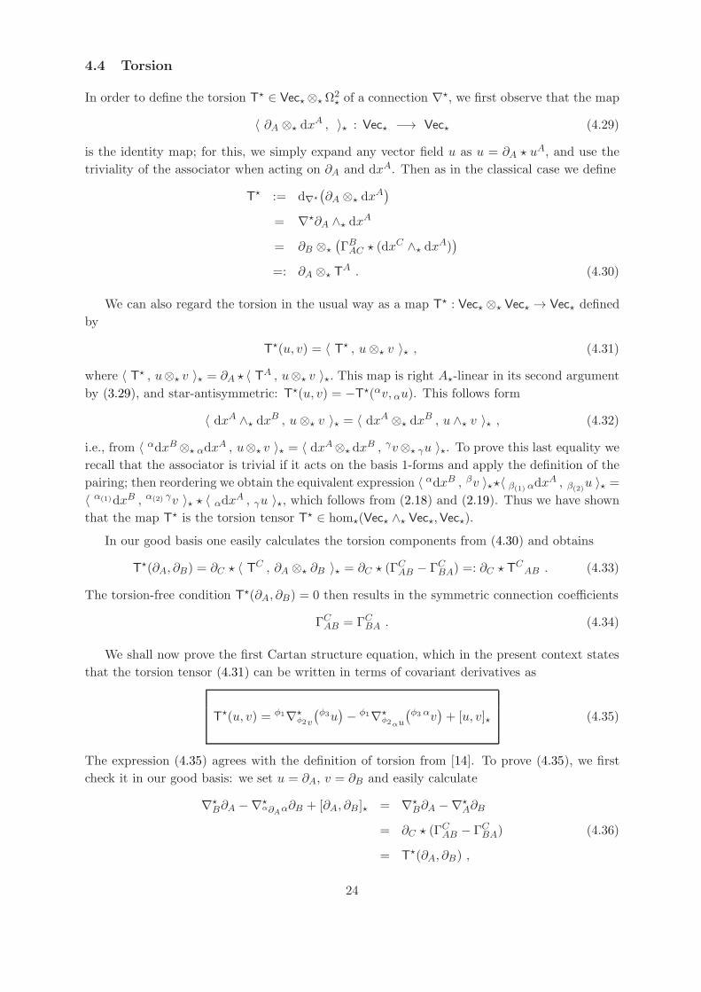
4.4 Torsion

In order to define the torsion T⋆ ∈ Vec⋆⊗⋆Ω2⋆ of a connection ∇⋆, we first observe that the map

〈 ∂A ⊗⋆ dxA , 〉⋆ : Vec⋆ −→ Vec⋆ (4.29)

is the identity map; for this, we simply expand any vector field u as u = ∂A ⋆ uA, and use the

triviality of the associator when acting on ∂A and dxA. Then as in the classical case we define

T⋆ := d∇⋆

(∂A ⊗⋆ dx

A)

= ∇⋆∂A ∧⋆ dxA

= ∂B ⊗⋆

(ΓBAC ⋆ (dx

C ∧⋆ dxA))

=: ∂A ⊗⋆ TA . (4.30)

We can also regard the torsion in the usual way as a map T⋆ : Vec⋆ ⊗⋆ Vec⋆ → Vec⋆ defined

by

T⋆(u, v) = 〈 T⋆ , u⊗⋆ v 〉⋆ , (4.31)

where 〈 T⋆ , u⊗⋆ v 〉⋆ = ∂A ⋆ 〈 TA , u⊗⋆ v 〉⋆. This map is right A⋆-linear in its second argument

by (3.29), and star-antisymmetric: T⋆(u, v) = −T⋆(αv, αu). This follows form

〈 dxA ∧⋆ dxB , u⊗⋆ v 〉⋆ = 〈 dxA ⊗⋆ dx

B , u ∧⋆ v 〉⋆ , (4.32)

i.e., from 〈 αdxB⊗⋆ αdxA , u⊗⋆ v 〉⋆ = 〈 dxA⊗⋆ dx

B , γv⊗⋆ γu 〉⋆. To prove this last equality we

recall that the associator is trivial if it acts on the basis 1-forms and apply the definition of the

pairing; then reordering we obtain the equivalent expression 〈 αdxB , βv 〉⋆⋆〈 β(1) αdxA , β(2)u 〉⋆ =

〈 α(1)dxB , α(2) γv 〉⋆ ⋆ 〈 αdxA , γu 〉⋆, which follows from (2.18) and (2.19). Thus we have shown

that the map T⋆ is the torsion tensor T⋆ ∈ hom⋆(Vec⋆ ∧⋆ Vec⋆,Vec⋆).

In our good basis one easily calculates the torsion components from (4.30) and obtains

T⋆(∂A, ∂B) = ∂C ⋆ 〈 TC , ∂A ⊗⋆ ∂B 〉⋆ = ∂C ⋆ (Γ

CAB − ΓCBA) =: ∂C ⋆ T

CAB . (4.33)

The torsion-free condition T⋆(∂A, ∂B) = 0 then results in the symmetric connection coefficients

ΓCAB = ΓCBA . (4.34)

We shall now prove the first Cartan structure equation, which in the present context states

that the torsion tensor (4.31) can be written in terms of covariant derivatives as

T⋆(u, v) = φ1∇⋆φ2v

(φ3u)− φ1∇⋆

φ2αu

(φ3 αv

)+ [u, v]⋆ (4.35)

The expression (4.35) agrees with the definition of torsion from [14]. To prove (4.35), we first

check it in our good basis: we set u = ∂A, v = ∂B and easily calculate

∇⋆B∂A −∇⋆

α∂Aα∂B + [∂A, ∂B ]⋆ = ∇⋆

B∂A −∇⋆A∂B

= ∂C ⋆ (ΓCAB − ΓCBA) (4.36)

= T⋆(∂A, ∂B) ,

24

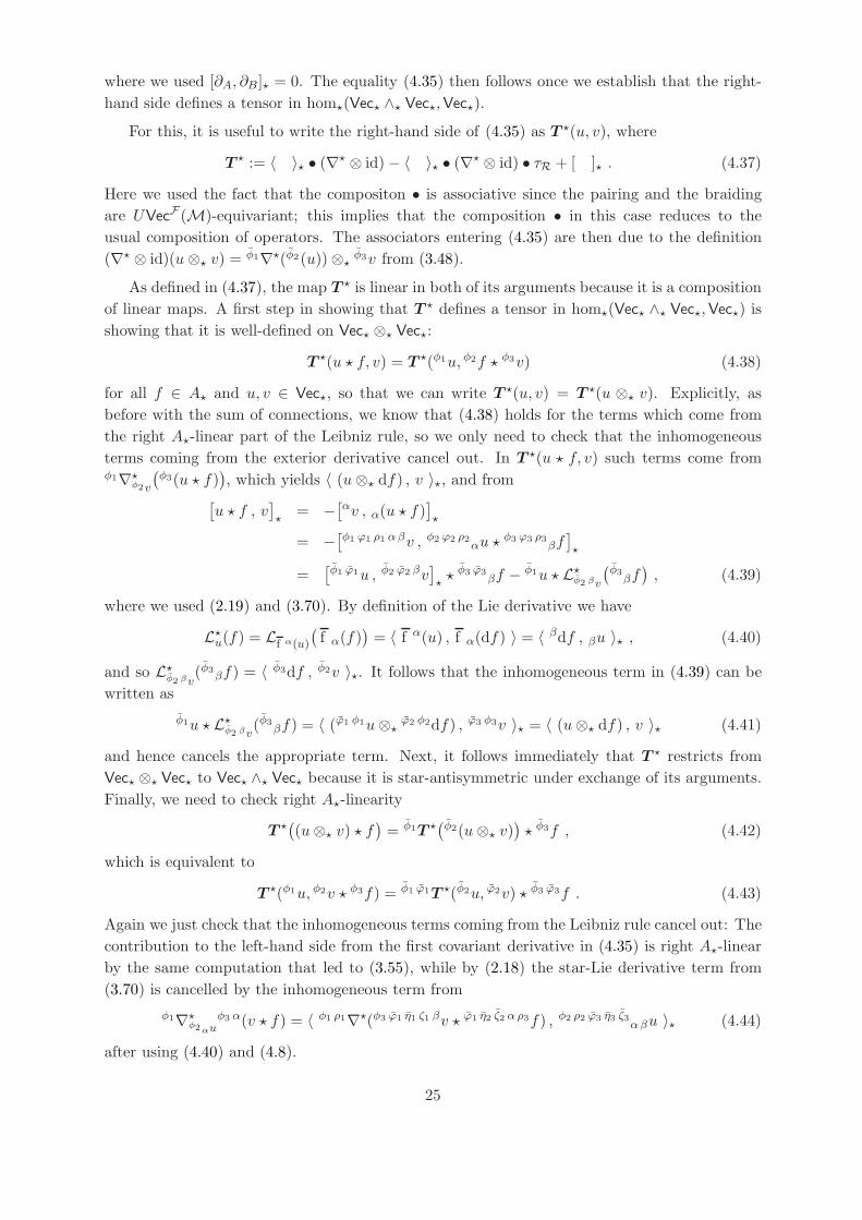
where we used [∂A, ∂B ]⋆ = 0. The equality (4.35) then follows once we establish that the right-

hand side defines a tensor in hom⋆(Vec⋆ ∧⋆ Vec⋆,Vec⋆).

For this, it is useful to write the right-hand side of (4.35) as T ⋆(u, v), where

T⋆ := 〈〉⋆ • (∇

⋆ ⊗ id)− 〈〉⋆ • (∇⋆ ⊗ id) • τR + [ ]⋆ . (4.37)

Here we used the fact that the compositon • is associative since the pairing and the braiding

are UVecF (M)-equivariant; this implies that the composition • in this case reduces to the

usual composition of operators. The associators entering (4.35) are then due to the definition

(∇⋆ ⊗ id)(u⊗⋆ v) =φ1∇⋆(φ2(u))⊗⋆

φ3v from (3.48).

As defined in (4.37), the map T ⋆ is linear in both of its arguments because it is a composition

of linear maps. A first step in showing that T ⋆ defines a tensor in hom⋆(Vec⋆ ∧⋆ Vec⋆,Vec⋆) is

showing that it is well-defined on Vec⋆ ⊗⋆ Vec⋆:

T⋆(u ⋆ f, v) = T

⋆(φ1u, φ2f ⋆ φ3v) (4.38)

for all f ∈ A⋆ and u, v ∈ Vec⋆, so that we can write T ⋆(u, v) = T ⋆(u ⊗⋆ v). Explicitly, as

before with the sum of connections, we know that (4.38) holds for the terms which come from

the right A⋆-linear part of the Leibniz rule, so we only need to check that the inhomogeneous

terms coming from the exterior derivative cancel out. In T ⋆(u ⋆ f, v) such terms come fromφ1∇⋆

φ2v

(φ3(u ⋆ f)

), which yields 〈 (u⊗⋆ df) , v 〉⋆, and from

[u ⋆ f , v

]⋆

= −[αv , α(u ⋆ f)

]⋆

= −[φ1 ϕ1 ρ1 αβv , φ2 ϕ2 ρ2

αu ⋆φ3 ϕ3 ρ3

βf]⋆

=[φ1 ϕ1u , φ2 ϕ2 βv

]⋆⋆ φ3 ϕ3

βf − φ1u ⋆ L⋆φ2 βv

(φ3βf), (4.39)

where we used (2.19) and (3.70). By definition of the Lie derivative we have

L⋆u(f) = Lf α(u)

(f α(f)

)= 〈 f α(u) , f α(df) 〉 = 〈 βdf , βu 〉⋆ , (4.40)

and so L⋆φ2 βv

(φ3βf) = 〈 φ3df , φ2v 〉⋆. It follows that the inhomogeneous term in (4.39) can be

written as

φ1u ⋆ L⋆φ2 βv(φ3βf) = 〈 (ϕ1 φ1u⊗⋆

ϕ2 φ2df) , ϕ3 φ3v 〉⋆ = 〈 (u⊗⋆ df) , v 〉⋆ (4.41)

and hence cancels the appropriate term. Next, it follows immediately that T ⋆ restricts from

Vec⋆ ⊗⋆ Vec⋆ to Vec⋆ ∧⋆ Vec⋆ because it is star-antisymmetric under exchange of its arguments.

Finally, we need to check right A⋆-linearity

T⋆((u⊗⋆ v) ⋆ f

)= φ1T

⋆(φ2(u⊗⋆ v)

)⋆ φ3f , (4.42)

which is equivalent to

T⋆(φ1u, φ2v ⋆ φ3f) = φ1 ϕ1T

⋆(φ2u, ϕ2v) ⋆ φ3 ϕ3f . (4.43)

Again we just check that the inhomogeneous terms coming from the Leibniz rule cancel out: The

contribution to the left-hand side from the first covariant derivative in (4.35) is right A⋆-linear

by the same computation that led to (3.55), while by (2.18) the star-Lie derivative term from

(3.70) is cancelled by the inhomogeneous term from

φ1∇⋆φ2αu

φ3 α(v ⋆ f) = 〈 φ1 ρ1∇⋆(φ3 ϕ1 η1 ζ1 βv ⋆ ϕ1 η2 ζ2 αρ3f) , φ2 ρ2 ϕ3 η3 ζ3αβu 〉⋆ (4.44)

after using (4.40) and (4.8).

25

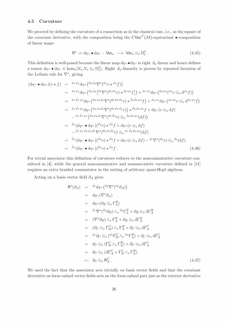
4.5 Curvature

We proceed by defining the curvature of a connection as in the classical case, i.e., as the square of

the covariant derivative, with the composition being the UVecF (M)-equivariant •-composition

of linear maps:

R⋆ := d∇⋆ • d∇⋆ : Vec⋆ −→ Vec⋆ ⊗⋆ Ω2⋆ . (4.45)

This definition is well-posed because the linear map d∇⋆•d∇⋆ is right A⋆-linear and hence defines

a tensor d∇⋆ • d∇⋆ ∈ hom⋆(V⋆, V⋆ ⊗⋆ Ω2⋆). Right A⋆-linearity is proven by repeated iteration of

the Leibniz rule for ∇⋆, giving

(d∇⋆ • d∇⋆)(v ⋆ f) = φ1 ϕ1d∇⋆

(φ2 ϕ2∇⋆(φ3v ⋆ ϕ3f)

)

= φ1 ϕ1d∇⋆

(φ2 ϕ2

[ρ1∇⋆(ρ2 φ3v) ⋆ ρ3 ϕ3f

])+ φ1 ϕ1d∇⋆

(φ2 ϕ2(φ3v ⊗⋆ d

ϕ3f))

= φ1 φ1 ϕ1d∇⋆

(φ2 ϕ2 ρ1∇⋆(ρ2 φ3 φ3v) ⋆ φ2 ρ3 ϕ3f

)+ φ1 ϕ1d∇⋆

(ϕ2 φ3v ⊗⋆ d

φ2 ϕ3f)

= φ1 φ1 ϕ1d∇⋆

(φ2 ϕ2 ρ1∇⋆(ρ2 φ3 φ3v)

)⋆ φ2 ρ3 ϕ3f + d∇⋆(v ⊗⋆ df)

− φ1 φ1 ϕ1(φ2 ϕ2 ρ1∇⋆(ρ2 φ3v)⊗⋆

φ2 ρ3 ϕ3(df))

= φ1(d∇⋆ • d∇⋆)(φ2v) ⋆ φ3f + d∇⋆(v ⊗⋆ df)

− φ1 ϕ1 φ2 ϕ2 ρ1∇⋆(ρ2 φ3 φ3v)⊗⋆φ1 φ2 ρ3 ϕ3(df)

= φ1(d∇⋆ • d∇⋆)(φ2v) ⋆ φ3f + d∇⋆(v ⊗⋆ df)−ρ1∇⋆(ρ2v)⊗⋆

ρ3(df)

= φ1(d∇⋆ • d∇⋆)(φ2v) ⋆ φ3f . (4.46)

For trivial associator this definition of curvature reduces to the noncommutative curvature con-

sidered in [4], while the general noncommutative and nonassociative curvature defined in [11]

requires an extra braided commutator in the setting of arbitrary quasi-Hopf algebras.

Acting on a basis vector field ∂A gives

R⋆(∂A) = φ1d∇⋆

(φ2∇⋆(φ3∂A)

)

= d∇⋆(∇⋆∂A)

= d∇⋆(∂B ⊗⋆ ΓBA)

= φ1∇⋆(φ2∂B) ∧⋆φ3ΓBA + ∂B ⊗⋆ dΓ

BA

= (∇⋆∂B) ∧⋆ ΓBA + ∂B ⊗⋆ dΓ

BA

= (∂C ⊗⋆ ΓCB) ∧⋆ Γ

BA + ∂C ⊗⋆ dΓ

CA

= φ1∂C ⊗⋆ (φ2ΓCB ∧⋆

φ3ΓBA) + ∂C ⊗⋆ dΓCA

= ∂C ⊗⋆ (ΓCB ∧⋆ Γ

BA) + ∂C ⊗⋆ dΓ

CA

= ∂C ⊗⋆ (dΓCA + ΓCB ∧⋆ Γ

BA)

=: ∂C ⊗⋆ RCA . (4.47)

We used the fact that the associator acts trivially on basis vector fields and that the covariant

derivative on form-valued vector fields acts on the form-valued part just as the exterior derivative

26

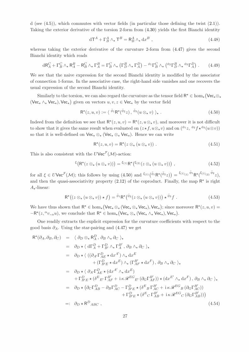
d (see (4.5)), which commutes with vector fields (in particular those defining the twist (2.1)).

Taking the exterior derivative of the torsion 2-form from (4.30) yields the first Bianchi identity

dTA + ΓAB ∧⋆ TB = RAB ∧⋆ dx

B , (4.48)

whereas taking the exterior derivative of the curvature 2-form from (4.47) gives the second

Bianchi identity which reads

dRCA + ΓCB ∧⋆ RBA − RCB ∧⋆ Γ

BA = ΓCB ∧⋆

(ΓBD ∧⋆ Γ

DA

)− φ1ΓCB ∧⋆

(φ2ΓBD ∧⋆

φ3ΓDA). (4.49)

We see that the naive expression for the second Bianchi identity is modified by the associator

of connection 1-forms. In the associative case, the right-hand side vanishes and one recovers the

usual expression of the second Bianchi identity.

Similarly to the torsion, we can also regard the curvature as the tensor field R⋆ ∈ hom⋆

(Vec⋆⊗⋆

(Vec⋆ ∧⋆ Vec⋆),Vec⋆)given on vectors u, v, z ∈ Vec⋆ by the vector field

R⋆(z, u, v) := 〈 φ1R⋆(φ2z) , φ3(u⊗⋆ v) 〉⋆ . (4.50)

Indeed from the definition we see that R⋆(z, u, v) = R⋆(z, u⊗⋆ v), and moreover it is not difficult

to show that it gives the same result when evaluated on (z⋆f, u⊗⋆v) and on (φ1z, φ2f ⋆φ3(u⊗v))

so that it is well-defined on Vec⋆ ⊗⋆ (Vec⋆ ⊗⋆ Vec⋆). Hence we can write

R⋆(z, u, v) = R⋆(z ⊗⋆ (u⊗⋆ v)) . (4.51)

This is also consistent with the UVecF (M)-action:

ξ(R⋆(z ⊗⋆ (u⊗⋆ v))

)= ξ(1)R⋆

(ξ(2)(z ⊗⋆ (u⊗⋆ v))

), (4.52)

for all ξ ∈ UVecF (M); this follows by using (4.50) and ξ(1)(φ1R⋆(φ2z)

)=

ξ(1)(1)φ1R⋆(

ξ(1)(2)φ2z),

and then the quasi-associativity property (2.12) of the coproduct. Finally, the map R⋆ is right

A⋆-linear:

R⋆((z ⊗⋆ (u⊗⋆ v)) ⋆ f

)= φ1R⋆

(φ2(z ⊗⋆ (u⊗⋆ v))

)⋆ φ3f . (4.53)

We have thus shown that R⋆ ∈ hom⋆

(Vec⋆⊗⋆ (Vec⋆⊗⋆Vec⋆),Vec⋆

); since moreover R⋆(z, u, v) =

−R⋆(z, αv, αu), we conclude that R⋆ ∈ hom⋆

(Vec⋆ ⊗⋆ (Vec⋆ ∧⋆ Vec⋆),Vec⋆

).

One readily extracts the explicit expression for the curvature coefficients with respect to the

good basis ∂A. Using the star-pairing and (4.47) we get

R⋆(∂A, ∂B , ∂C) = 〈 ∂D ⊗⋆ RDA , ∂B ∧⋆ ∂C 〉⋆

= ∂D ⋆ 〈 dΓDA + ΓDB′ ∧⋆ Γ

B′

A , ∂B ∧⋆ ∂C 〉⋆

= ∂D ⋆ 〈 ((∂A′ΓDAE ⋆ dxA′

) ∧⋆ dxE

+(ΓDB′E ⋆ dxE) ∧⋆ (Γ

B′

AF ⋆ dxF ) , ∂B ∧⋆ ∂C 〉⋆

= ∂D ⋆ 〈 ∂A′ΓDAE ⋆ (dxA′

∧⋆ dxE)

+ΓDB′E ⋆ (δEE′ ΓB

′

AF + i κREG

E′ (∂GΓB′

AF )) ⋆ (dxE′

∧⋆ dxF ) , ∂B ∧⋆ ∂C 〉⋆

= ∂D ⋆(∂CΓ

DAB − ∂BΓ

DAC − ΓDB′E ⋆ (δ

EB ΓB

′

AC + i κREG

B (∂GΓB′

AC))

+ΓDB′E ⋆ (δEC ΓB

′

AB + iκREG

C (∂GΓB′

AB)))

=: ∂D ⋆ RDABC , (4.54)

27

where once again we used the fact that the associator acts trivially on the basis vectors and

basis 1-forms.

We shall now prove the second Cartan structure equation, which in the present context states

that the curvature tensor (4.50) can be written in terms of covariant derivatives as

R⋆(z, u, v) = κ1 φ1 φ′1∇

⋆ρ3 ζ3 φ3 φ′3v

(ρ1 φ1 κ2 φ2 φ

′2∇

⋆ρ2 ζ2 φ3u

ζ1 φ2 κ3z)

− κ1 φ1 φ′1∇

⋆ρ3 ζ3 φ3 φ′

3αu

(ρ1 φ1 κ2 φ2 φ

′2∇

⋆ρ2 ζ2 φ3αv

ζ1 φ2 κ3z)+∇

⋆[u,v]⋆

z(4.55)

where to streamline the notation we introduced the bold-face covariant derivative

∇⋆vu := 〈 φ1∇⋆(φ2u) , φ3v 〉⋆ . (4.56)

The expression (4.55) for the curvature agrees with that of [14] after taking into account their

different conventions;1 for trivial associator it reduces to the general expression in [6]. To prove

(4.55) we first check it on our good basis by setting z = ∂A, u = ∂B and v = ∂C . Then the

right-hand side reduces to

∇⋆C(∇

⋆B∂A)−∇⋆

α∂B(∇⋆

α∂C∂A) +∇⋆

[∂B,∂C ]⋆∂A

= ∇⋆C(∇

⋆B∂A)−∇⋆

B(∇⋆C∂A)

= ∇⋆C(∂D ⋆ Γ

DAB)−∇⋆

B(∂D ⋆ ΓDAC)

= 〈 ∇⋆∂D ,α∂C 〉⋆ ⋆ αΓ

DAB + ∂D ⋆ 〈 dΓ

DAB , ∂C 〉⋆

−〈 ∇⋆∂D ,α∂B 〉⋆ ⋆ αΓ

DAC − ∂D ⋆ 〈 dΓ

DAC , ∂B 〉⋆

= R⋆(∂A, ∂B , ∂C) , (4.57)

where in the third equality we used the Leibniz rule (4.8) while the last equality follows from

(4.54). The equality (4.55) for arbitrary vectors then follows once we establish that the right-

hand side defines a tensor in hom⋆(Vec⋆ ⊗⋆ (Vec⋆ ∧⋆ Vec⋆),Vec⋆).

For this, as in the case of the torsion, we rewrite the right-hand side of (4.55) as a trilinear

map R⋆ on vectors z, u and v, and prove that it is a map in hom⋆(Vec⋆⊗⋆ (Vec⋆∧⋆Vec⋆),Vec⋆).

To arrive at the form of R⋆, for notational clarity we first consider vectors z, u, v on which the

associator acts trivially (for example basis vectors ∂A, ∂B , ∂C). Then we reproduce ∇⋆v(∇

⋆u z) as

the elementary compositions

z ⊗⋆ (u⊗⋆ v)∇⋆⊗⋆ id⊗⋆2

7−−−−−−−→ ∇⋆z ⊗⋆ (u⊗⋆ v)Φ−1

7−−→ (∇⋆z ⊗⋆ u)⊗⋆ v (4.58)

〈〉⋆⊗⋆ id7−−−−−−−→ ∇⋆

uz ⊗⋆ v∇⋆⊗⋆ id7−−−−−→ ∇⋆(∇⋆

u z)⊗⋆ v〈〉⋆7−−−→ ∇⋆

v(∇⋆u z) .

This leads to a definition of R⋆ written solely in terms of the connection ∇⋆, the associator Φ−1,

and the equivariant maps studied in Section 3, which reads as

R⋆ := 〈〉⋆ • (∇

⋆ ⊗ id) • (〈〉⋆ ⊗ id) • Φ−1Vec⋆⊗Ω1

⋆,Vec⋆,Vec⋆• (∇⋆ ⊗ id⊗2) • (id⊗3 − id⊗R τR)

+ 〈〉⋆ • (∇⋆ ⊗ id) • (id⊗R [ ]⋆) . (4.59)

1We are grateful to Michael Fuchs for pointing this out to us.

28

Even though the composition • is nonassociative, there is no ambiguity in this definition because

of the equivariance of the maps which are composed and because φaφb = 0 (the associator

being generated by an abelian subalgebra). For these same reasons, there is the more explicit

expression

R⋆ = 〈〉⋆ (

φ1∇⋆ ⊗ id) (〈〉⋆ ⊗ id) Φ−1Vec⋆⊗Ω1

⋆,Vec⋆,Vec⋆ (φ2∇⋆ ⊗ id⊗2) φ3 (id

⊗3− id⊗ τR)

+ 〈〉⋆ (∇⋆ ⊗ id) (id⊗ [ ]⋆) . (4.60)

As sought, explicit evaluation of R⋆ on z ⊗⋆ (u⊗⋆ v) gives the right-hand side of (4.55):

R⋆(z, u, v) = 〈 η1 φ1∇⋆ η2〈 ρ1(ϕ1 φ2∇⋆ϕ2 φ3(1) z) ,

ρ2 ϕ3(1)φ3(2)(1) u 〉⋆ ,

η3 ρ3 ϕ3(2)φ3(2)(2) v 〉⋆

−〈 η1 φ1∇⋆ η2〈 ρ1(ϕ1 φ2∇⋆ϕ2 φ3(1) z) ,ρ2 ϕ3(1)

φ3(2)(1) αv 〉⋆ ,η3 ρ3 ϕ3(2)

φ3(2)(2)αu 〉⋆

+ 〈 ϕ1∇⋆ϕ2z , ϕ3 [u, v]⋆ 〉⋆

= 〈 η1 κ1 φ1 φ′1∇⋆ η2〈 ρ1 ϕ1 φ1 κ2 φ2 φ

′2∇⋆ζ1 ϕ2 φ2 κ3z , ρ2 ζ2 ϕ3 φ3u 〉⋆ ,

η3 ρ3 ζ3 φ3 φ′3v 〉⋆

−〈 η1 κ1 φ1 φ′1∇⋆ η2〈 ρ1 ϕ1 φ1 κ2 φ2 φ

′2∇⋆ζ1 ϕ2 φ2 κ3z , ρ2 ζ2 ϕ3 φ3αv 〉⋆ ,

η3 ρ3 ζ3 φ3 φ′3αu 〉⋆

+ 〈 ϕ1∇⋆ϕ2z , ϕ3 [u, v]⋆ 〉⋆ . (4.61)

Now the proof that R⋆ is a map in hom⋆(Vec⋆⊗⋆ (Vec⋆∧⋆Vec⋆),Vec⋆) requires as a first step

to show that it is a well-defined map on Vec⋆ ⊗⋆ (Vec⋆ ⊗⋆ Vec⋆):

R⋆(z, u ⋆ f, v) = R

⋆(z, φ1u, φ2f ⋆ φ3v) , (4.62)

so that we get a well-defined map R⋆(z, u ⊗⋆ v) = R⋆(z, u, v), and

R⋆(z ⋆ f, u⊗⋆ v) = R

⋆(φ1z, φ2f ⋆ φ3(u⊗⋆ v)) , (4.63)

so that we get a well-defined map R⋆(z ⊗⋆ (u ⊗⋆ v)) = R⋆(z, u, v). The star-antisymmetry of

R⋆ under u ⊗⋆ v → αv ⊗⋆ αu then immediately follows, and this implies that R⋆ is a linear

map from Vec⋆ ⊗⋆ (Vec⋆ ∧⋆ Vec⋆) to Vec⋆. The final step is to show that R⋆ ∈ hom⋆(Vec⋆ ⊗⋆

(Vec⋆∧⋆,Vec⋆),Vec⋆), i.e., that it is right A⋆-linear:

R⋆((z ⊗⋆ (u⊗⋆ v)) ⋆ f

)= φ1R

⋆(φ2(z ⊗⋆ (u⊗⋆ v))

)⋆ φ3f . (4.64)

In the following we prove right A⋆-linearity (4.64); the remaining A⋆-linearity properties (4.62)

and (4.63) can be established with similar techniques.

For this, we note again that if the star-connection ∇⋆ and the star-Lie derivative L⋆ =

[ ]⋆ were right A⋆-linear maps, then the operator (4.59) would also be right A⋆-linear because

all composite maps would be right A⋆-linear. Hence as before it suffices to check that the

inhomogeneous terms coming from the Leibniz rule for the connection and the Lie derivative

cancel out. We denote by Leib⋆ the projector onto the inhomogeneous terms. For example

Leib⋆(∇⋆(u ⋆ f)

)= u⊗⋆ df , (4.65)

which induces

Leib⋆(∇⋆v(u ⋆ f)

)= 〈 Leib⋆(∇⋆(u ⋆ f)) , v 〉⋆ =

ϕ1u ⋆ 〈 ϕ2df , ϕ3v 〉⋆ = Leib⋆(∇⋆v(u ⋆ f)

).(4.66)

29

Here we used the fact that in the inhomogeneous term the covariant derivative ∇⋆v from (4.56)

acts as a rescaled exterior derivative φ1d = ǫ(φ1) d, which is UVecF (M)-equivariant. Further-

more, from (4.39) we also have

Leib⋆([u ⋆ f, v]⋆

)= φ1u ⋆ 〈 φ3df , φ2v 〉⋆ . (4.67)

The projector Leib⋆ in these examples is a linear operator in u, v and f . We have to show that

Leib⋆(R⋆((z ⊗⋆ (v ⊗⋆ u)) ⋆ f

))= 0 for all z, v, u ∈ Vec⋆ and f ∈ A⋆. Since

(z ⊗⋆ (v ⊗⋆ u)

)⋆ f = ϕ1 ρ1z ⊗⋆

((ϕ2v ⊗⋆

ρ2u) ⋆ ϕ3 ρ3f)

= ϕ1 ρ1z ⊗⋆

(ζ1 ϕ2v ⊗⋆ (

ζ2 ρ2u ⋆ ζ2 ϕ3 ρ3f)), (4.68)

this condition is equivalent to Leib⋆(R⋆(z⊗⋆ (v⊗⋆ (u⋆f))

))= 0 because of linearity in z, v, u, f .

Hence we check that Leib⋆(R⋆(z, v, u ⋆ f)

)= 0, or equivalently, using star-antisymmetry and

linearity again, that Leib⋆(R⋆(z, u ⋆ f, v)

)= 0.

From (4.55) we write

Leib⋆(R⋆(z, u ⋆ f, v)

)= Leib⋆

(κ1 φ1 φ

′1∇

⋆ρ3 ζ3 φ3 φ′

3v

(ρ1 φ1 κ2 φ2 φ

′2∇

⋆ρ2 ζ2 φ3 (u⋆f)

ζ1 φ2 κ3z))

+ Leib⋆(∇⋆[u⋆f,v]⋆

z)

(4.69)

and compare the two contributions. The second contribution in (4.69) is equal to

∇⋆Leib

⋆([u⋆f,v]⋆)z = −∇

⋆φ1u⋆〈 φ3df , φ2v 〉⋆

z

= −(κ1 ϕ1∇

⋆κ2

¯φ2 φ1u

¯φ1 ϕ2z)⋆ κ3

¯φ3 ϕ3〈 φ3df , φ2v 〉⋆ , (4.70)

where in the second equality we used the definition (4.56) to rewrite

∇⋆u⋆fz = 〈 φ1 ϕ1∇⋆φ2 ϕ2z , φ3u ⋆ ϕ3f 〉⋆

= 〈 φ′1(φ1 ϕ1∇⋆φ2 ϕ2z) , φ

′2 φ3u 〉⋆ ⋆

φ′3 ϕ3f

=(κ1 ϕ1∇

⋆κ2

¯φ2u

¯φ1 ϕ2z)⋆ κ3

¯φ3 ϕ3f , (4.71)

and then replace u⋆f with φ1u⋆ 〈 φ3df , φ2v 〉⋆. The first contribution in (4.69) can be rewritten

without the first three associator legs κa, φa, φ′a, because in the inhomogeneous term the covariant

derivative κ1 φ1 φ′1∇

⋆w again acts as a rescaled exterior derivative κ1 φ1 φ

′1d = ǫ(κ1) ǫ(φ1) ǫ(φ

′1) d,

which is UVecF (M)-equivariant. Therefore the first contribution in (4.69) equals

Leib⋆(∇⋆ρ3 φ′3 ζ3 η3 φ3v

(ρ1 φ

′1 φ1∇

⋆ρ2 ζ2u⋆φ

′2 η2f

ζ1 η1 φ2z))

= Leib⋆(∇⋆ρ3 φ′

3ζ3 η3 φ3v

((κ1 ϕ1 ρ1 φ

′1 φ1∇

⋆κ2

¯φ2 ρ2 ζ2u

¯φ1 ϕ2 ζ1 η1 φ2z) ⋆ κ3¯φ3 ϕ3 φ

′2 η2f

))(4.72)

= χ1(κ1 ϕ1 ρ1 φ

′1 φ1∇

⋆κ2

¯φ2 ρ2 ζ2u

¯φ1 ϕ2 ζ1 η1 φ2z)⋆ 〈 χ2 κ3

¯φ3 ϕ3 φ′2 η2df , χ3 ρ3 φ

′3 ζ3 η3 φ3v 〉⋆ .

Replacing (u, f, v) with (η1u, η2f, η3v) in (4.72) gives an action of φ′1⊗ η1⊗ ζ1⊗ φ′2 ζ2 η2⊗ φ

′3 ζ3 η3

which cancels against that of((∆F ⊗ id)∆F (χ1)

)⊗ χ2 ⊗ χ3 and yields

(κ1 ϕ1 ρ1 φ1∇

⋆κ2

¯φ2 ρ2 ζ2u

¯φ1 ϕ2 ζ1 φ2z)⋆ 〈 κ3

¯φ3 ϕ3df , ρ3 ζ3 φ3v 〉⋆ (4.73)

=(κ1 ϕ1∇

⋆κ2

¯φ2u

¯φ1 ϕ2z)⋆ κ3

¯φ3 ϕ3〈 df , v 〉⋆ ,

30

thereby cancelling the contribution (4.70) with the same replacement of (u, f, v). This shows

that

Leib⋆(R⋆(z, η1u ⋆ η2f, η3v)

)= 0 (4.74)

and hence establishes the right A⋆-linearity property (4.64) as required.

4.6 Ricci tensor

Since the associator acts trivially on the basis dxA and its dual ∂A, the definition of the Ricci

tensor can be given following the noncommutative case studied in [6]. We define

Ric⋆(u, v) := −〈 R⋆(u, v, ∂A) , dxA 〉⋆ , (4.75)

for all u, v ∈ Vec⋆, where the pairing between a vector field on the left and a form on the right

is given by

〈 u , ω 〉⋆ = 〈 f α(u) , f α(ω) 〉 , (4.76)

similarly to (3.27). The properties of this pairing are completely analogous to those described in

Section 3.5, by simply interchanging forms and vector fields in all expressions considered there.

We now show that the map (4.75) defines a tensor Ric⋆ ∈ hom⋆(Vec⋆⊗⋆Vec⋆,Vec⋆). We first

prove that it is a map from Vec⋆⊗⋆ Vec⋆ to Vec⋆, so that we can write Ric⋆(u, v) = Ric⋆(u⊗⋆ v);

indeed, we have

Ric⋆(u ⋆ f, v) = −〈 R⋆(u ⋆ f, v, ∂A) , dxA 〉⋆

= −〈 R⋆((u ⋆ f)⊗⋆ (v ⊗⋆ ∂A)) , dxA 〉⋆

= −〈 R⋆(φ1u⊗⋆ (φ2f ⋆ φ3(v ⊗⋆ ∂A))) , dx

A 〉⋆

= −〈 R⋆(φ1u⊗⋆ ((φ2f ⋆ φ3v)⊗⋆ ∂A)) , dx

A 〉⋆

= Ric⋆(φ1u, φ2f ⋆ φ3v) (4.77)

where in the second equality we used (4.51), and in the fourth equality the fact that the associator

acts trivially on ∂A. Next we prove compatibility with the UVecF (M)-action:

ξ(Ric⋆(u⊗⋆ v)

)= ξ(1)Ric⋆

(ξ(2)(u⊗ v)

), (4.78)

which follows from (4.52), iterated use of (2.12) and from ξ(∂A ⊗⋆ dxA) = ǫ(ξ) ∂A ⊗⋆ dx

A; this

latter property follows from writing the identity map id : Vec⋆ → Vec⋆ as in (4.29) and usingξid = ǫ(ξ) id, i.e., ξ

(id(u)

)= ξ(1) id(ξ(2)u) = id(ξu), for all ξ ∈ UVecF (M) and u ∈ Vec⋆. Finally,

we prove right A⋆-linearity. For this, we notice that

φ1u⊗⋆

((φ2v ⋆ φ3f)⊗⋆ ∂A

)= φ1u⊗⋆

(φ2v ⊗⋆ (

α∂A ⋆ αφ3f)

)

= φ1u⊗⋆

((φ2v ⊗⋆

α∂A) ⋆φ3αf)

=(ϕ1 φ1u⊗⋆

ϕ2(φ2v ⊗⋆α∂A)

)⋆ ϕ3 φ3

αf

=(u⊗⋆ (v ⊗⋆

α∂A))⋆ αf (4.79)

where we used the fact that the associator commutes with each leg of the R-matrix and hence

it acts trivially on α∂A. Then the proof follows from (4.79) and the centrality of the tensor

31

∂A ⊗⋆ dxA: f ⋆ (∂A ⊗⋆ dx

A) = (α∂A ⊗⋆βdxA) ⋆ β αf = (∂A ⊗⋆ dx

A) ⋆ f , see (3.16) and (3.23), or

again (4.29). Explicitly, we have

Ric⋆((u⊗⋆ v) ⋆ f

)= Ric⋆

(φ1u⊗⋆ (

φ2v ⋆ φ3f))

= −〈 R⋆(φ1u⊗⋆ ((

φ2v ⋆ φ3f)⊗⋆ ∂A)), dxA 〉⋆

= −〈 R⋆((u⊗⋆ (v ⊗⋆

α∂A)) ⋆ αf), dxA 〉⋆

= −〈 ϕ1R⋆(ϕ2(u⊗⋆ (v ⊗⋆

α∂A)))⋆ ϕ3

αf , dxA 〉⋆

= −〈 ϕ1(R⋆(ϕ2(u⊗⋆ (v ⊗⋆

α∂A))))⋆ ϕ3

αf , dxA 〉⋆

= −〈 ϕ1 ρ1(R⋆(ϕ2u⊗⋆ (

ρ2v ⊗⋆α∂A)

)), ϕ3 ρ3

αf ⋆ dxA 〉⋆

= −〈 ϕ1 ρ1(R⋆(ϕ2u⊗⋆ (

ρ2v ⊗⋆α∂A)

)), βdxA 〉⋆ ⋆ β α

ϕ3 ρ3f

= −ϕ1 ρ1〈 R⋆(ϕ2u⊗⋆ (

ρ2v ⊗⋆ ∂A)), dxA 〉⋆ ⋆

ϕ3 ρ3f

= ϕ1 ρ1Ric⋆(ϕ2u⊗⋆

ρ2v)⋆ ϕ3 ρ3f

= ϕ1Ric⋆(ϕ2(u⊗⋆ v)

)⋆ ϕ3f . (4.80)

The coefficients of the Ricci tensor in the coordinate basis are given by

Ric⋆ = RicAD ⋆ (dxD ⊗⋆ dx

A) , (4.81)

where RicBC := Ric⋆(∂B , ∂C); indeed we have

Ric⋆(∂B , ∂C) = 〈 RicAD ⋆ (dxD ⊗⋆ dx

A) , ∂B ⊗⋆ ∂C 〉⋆ = RicBC . (4.82)

We use (4.54) together with the fact that the associator acts trivially on basis vectors and basis

1-forms to calculate explicitly

RicBC = −〈 R⋆(∂B , ∂C , ∂A) , dxA 〉⋆

= −〈 ∂D ⋆ RDBCA , dx

A 〉⋆

= −αRDBCA ⋆ 〈 α∂D , dxA 〉⋆

= RABAC − i κREF

D ∂ERDBCA ⋆ 〈 ∂F , dx

A 〉⋆

= RABAC − i κREA

D ∂ERDBCA

= ∂AΓABC − ∂CΓ

ABA + ΓAB′A ⋆ Γ

B′

BC − ΓAB′C ⋆ ΓB′

BA

+ iκΓAB′E ⋆(REG

A (∂GΓB′

BC)− REG

C (∂GΓB′

BA))

+ iκREG

A ∂G∂CΓABE − iκR

EGA ∂G

(ΓAB′E ⋆ Γ

B′


BE

)

+κ2 RAF

D

(REG

A ∂F (ΓDB′E ⋆ ∂GΓ

B′

BC)− REG

C ∂F (ΓDB′E ⋆ ∂GΓ

B′

BA)). (4.83)

This calculation did not use symmetry of ΓABC , i.e., the torsion-free condition (4.34). Indeed

this is the Ricci tensor of an arbitrary affine connection.

32

5 Nonassociative Riemannian geometry and gravity

5.1 Metric and torsion-free connection conditions

We shall now discuss the metric aspects of nonassociative differential geometry and how it can be

used to build a theory of nonassociative gravity. For this, notice first of all that star-symmetric

tensors are of the form T ⊗⋆ T′ + αT ′ ⊗⋆ αT . A metric tensor is an element g⋆ ∈ Ω1

⋆ ⊗⋆ Ω1⋆

which can be written in the basis dxA as g⋆ = gAB ⋆ (dxA⊗⋆ dx

B) with real-valued components

gAB = gBA ∈ A⋆ (the bracketing here is immaterial due to the basis 1-forms). We can regard it

as a map g⋆ ∈ hom⋆(Vec⋆ ⊗⋆ Vec⋆, A⋆) which on vector fields u, v ∈ Vec⋆ gives the function

g⋆(u, v) = 〈 g⋆ , u⊗⋆ v 〉⋆ . (5.1)

It is star-symmetric: g⋆(u, v) = g⋆(αv, αu), and one easily confirms that g⋆(∂A, ∂B) = gAB . As

usual we assume that g⋆ is nondegenerate: g⋆(u, v) = 0 for all v ∈ Vec⋆ if and only if u = 0.

Let us now study the metric compatibility condition for a connection ∇⋆ : Vec⋆ → Vec⋆⊗⋆Ω1⋆.

The connection ∇⋆ gives a connection ∇⋆ : Vec⋆ ⊗⋆ Vec⋆ → (Vec⋆ ⊗⋆ Vec⋆)⊗⋆ Ω1⋆ on the tensor

product Vec⋆⊗ ⋆Vec⋆, defined as in Section 4.3. The space Ω1⋆⊗⋆Ω

1⋆ is dual to Vec⋆⊗⋆ Vec⋆ and

hence ∇⋆ : Vec⋆ ⊗⋆ Vec⋆ → (Vec⋆ ⊗⋆ Vec⋆) ⊗⋆ Ω1⋆ induces a dual connection ⋆∇ : Ω1

⋆ ⊗⋆ Ω1⋆ →

(Ω1⋆ ⊗⋆ Ω

1⋆)⊗⋆ Ω

1⋆ as in (4.14), now with ω ∈ Ω1

⋆ ⊗⋆ Ω1⋆ and u ∈ Vec⋆ ⊗⋆ Vec⋆. We can then state

the metric compatibility condition as⋆∇g⋆ = 0 . (5.2)

We shall now show that, as in the classical case, this condition together with the torsion-free

condition uniquely determine the connection in terms of the metric.

We start by using (4.14) with ω = g⋆ ∈ Ω1⋆ ⊗⋆ Ω

1⋆ and u = ∂A ⊗⋆ ∂B ∈ Vec⋆ ⊗⋆ Vec⋆ to get

dgAB = d〈 g⋆ , ∂A ⊗⋆ ∂B 〉⋆

= 〈 ⋆∇g⋆ , ∂A ⊗⋆ ∂B 〉⋆ + 〈 φ1g⋆ , φ2∇⋆(φ3(∂A ⊗⋆ ∂B)) 〉⋆

= 〈 g⋆ , ∇⋆(∂A ⊗⋆ ∂B) 〉⋆ , (5.3)

where we used gAB = gBA and the fact that the associators act trivially on the basis vectors.

We can write this more explicitly as

dgAB = 〈 g⋆ , ∇⋆∂A ⊗⋆ ∂B + α∂A ⊗⋆ α∇⋆∂B 〉⋆

= 〈 g⋆ , ∇⋆∂A ⊗⋆ ∂B + αγ∂A ⊗⋆ α∇⋆γ∂B 〉⋆

= 〈 g⋆ , ∇⋆∂A ⊗⋆ ∂B + α∂A ⊗⋆ α(∇⋆∂B) 〉⋆

= 〈 g⋆ , (∂C ⊗⋆ ΓCA)⊗⋆ ∂B + α∂A ⊗⋆ α(∂D ⊗⋆ Γ

DB ) 〉⋆

= 〈 g⋆ , (∂C ⊗⋆ ΓCA)⊗⋆ ∂B + α∂A ⊗⋆ (∂D ⊗⋆ αΓ

DB ) 〉⋆

= 〈 g⋆ , ∂C ⊗⋆ (α∂B ⊗⋆ αΓ

CA) +

α∂A ⊗⋆ (∂D ⊗⋆ αΓDB ) 〉⋆

= 〈 g⋆ , ∂C ⊗⋆ (α∂B ⊗⋆ αΓ

CA) + ∂D ⊗⋆ (

α∂A ⊗⋆ αΓDB ) 〉⋆

= 〈 g⋆ , ∂C ⊗⋆ (α∂B ⊗⋆ αΓ

CA + α∂A ⊗⋆ αΓ

CB) 〉⋆

= 〈 gMC ⋆ dxM , α∂B ⊗⋆ αΓ

CA + α∂A ⊗⋆ αΓ

CB 〉⋆

= gMN ⋆(〈 dxM , α∂B 〉⋆ ⋆ αΓ

NA + 〈 dxM , α∂A 〉⋆ ⋆ αΓ

NB

), (5.4)

33

where in the first equality we used (4.23) and the fact that the R-matrix acts trivially on

a pair of basis vectors, so that β∂A ⊗⋆ β∂B = ∂A ⊗⋆ ∂B . In the second equality we usedξ(∇⋆∂B) = ξ(1)∇⋆(ξ(2)∂B) (as for all linear maps acting from the left), the coproduct action

(2.19) on the R-matrix, and again triviality of the action of R as well as of the associator

on ∂A ⊗⋆ ∂B . In the sixth line we used the fact that α∂A is again a basis vector and then

star-symmetry of the metric.

We similarly calculate

〈 dxM , α∂B 〉⋆ ⋆ αΓNA = 〈 dxM , α∂B 〉⋆ ⋆ α(Γ

NAC ⋆ dx

C)

= 〈 dxM , β γ∂B 〉⋆ ⋆ βΓNAC ⋆ γdx

C

= 〈 dxM , β∂B 〉⋆ ⋆(βΓ

NAC ⋆ dx

C)

=(〈 dxM , β∂B 〉⋆ ⋆ βΓ

NAC

)⋆ dxC

= 〈 dxM , ΓNAC ⋆ ∂B 〉⋆ ⋆ dxC , (5.5)

where as usual we used again (2.19) together with α∂A ⋆ αdxB = ∂A ⋆ dx

B for our cochain twist

(2.1). We can finally write

dgAB = gMN ⋆ 〈 dxM , ΓNAC ⋆ ∂B 〉⋆ ⋆ dxC + gMN ⋆ 〈 dxM , ΓNBC ⋆ ∂A 〉⋆ ⋆ dx

C . (5.6)

We now contract the expression (5.6) with ∂D using the star-pairing to obtain

∂DgAB = 〈 dgAB , ∂D 〉⋆ = gMN ⋆(〈 dxM , ΓNAD ⋆ ∂B 〉⋆ + 〈 dxM , ΓNBD ⋆ ∂A 〉⋆

). (5.7)

We write the expression (5.7) two more times, with the indices A,B,D cyclically permuted,

and consider the combination ∂DgAB + ∂AgBD − ∂BgDA. Using the fact that the connection

coefficients are symmetric for vanishing torsion (see (4.34)), we obtain

gMN ⋆ 〈 dxM , ΓNAD ⋆ ∂B 〉⋆ =12 (∂DgAB + ∂AgBD − ∂BgAD) . (5.8)

The left hand side equals 〈 gMN ⋆ dxM ⋆ ΓNAD , ∂B〉⋆, so star-multiplying (5.8) by any vB ∈ A⋆

gives

〈 gMN ⋆ dxM ⋆ ΓNAD , v 〉⋆ =12 (∂DgAB + ∂AgBD − ∂BgAD) ⋆ v

B , (5.9)

with v = ∂B ⋆ vB ∈ Vec⋆. Since the vector field v is arbitrary and the star-pairing is nondegen-

erate, this shows that

gMN ⋆ dxM ⋆ ΓNAD = 12 (∂DgAB + ∂AgBD − ∂BgAD) ⋆ dx

B . (5.10)

Since moreover the metric g⋆ is nondegenerate, the expression (5.10) uniquely defines the torsion-

free metric compatible connection in the nonassociative case.

It remains to explicitly solve for the connection coefficients ΓNAD from (5.10). For this, we

use (3.16) to rewrite (5.10) as

dxM ⋆ GMN ⋆ ΓNAD = dxM ⋆ 12

(∂DgAM + ∂AgMD − ∂MgAD

+ iκREF

M (∂E∂DgAF + ∂E∂AgDF )), (5.11)

with

GMN = gMN + iκREF

M ∂EgNF , (5.12)

34

where the associators act trivially due to the basis vector fields and basis 1-forms. The tensor

GMN is nondegenerate but not symmetric; it can be thought of as a realisation the R-flux

corrected “effective metric” anticipated from the string theory perspective [14]. We then use the

star-pairing to contract (5.11) from the left with ∂C and obtain

GCN ⋆ ΓNAD = 12

(∂DgAC + ∂AgDC − ∂CgAD + iκR

EFC (∂E∂DgAF + ∂E∂AgDF )

). (5.13)

We are now faced with the problem of extracting the connection coefficients ΓNAD from (5.13).

5.2 Inversion in A⋆

Before tackling the matrix equation (5.13), let us consider a simpler problem involving ordinary

functions: Start from the equation

h ⋆ g = w , (5.14)

where h, g, w ∈ A⋆ are functions, the star-product is given by (3.6), and h is invertible with

respect to the usual pointwise product of functions. From (5.14) we would like to uniquely

determine g in terms of h and w.

Recalling the factorization (2.3) of the cochain twist F , let ∗ := ⋆F be the star-product

induced by the twist F from (2.4); this is of course just the canonical associative Moyal-Weyl

star-product on phase space: f ∗g = f α(f) ·f α(g). All the R-flux dependence is contained in the

twist FR from (2.5). Let h−1 be the usual pointwise inverse of the function h: h−1·h = h·h−1 = 1.

Then h is also ∗-invertible [7], and we write h∗−1 for the ∗-inverse function:

h∗−1 ∗ h = h ∗ h∗−1 = 1 . (5.15)

It can be expressed explicitly as a power series [7]

h∗−1 = h−1 +∞∑

n=1

h−1 ∗(1− h ∗ h−1

)∗n, (5.16)

where, since(1 − h ∗ h−1

)∗nis of order O(~n), in order to get h∗−1 up to order O(~n) we only

have to compute the finite sum h−1 +∑n

k=1 h−1 ∗

(1− h ∗ h−1

)∗k. This enables one to uniquely

determine the function h∗−1 order by order in ~. If no R-flux is present, the equation (5.14)

becomes h ∗ g = w which has the unique solution

g = 1 ∗ g = (h∗−1 ∗ h) ∗ g = h∗−1 ∗ (h ∗ g) = h∗−1 ∗ w . (5.17)

In the absence of R-flux, the problem of determining g from the functions h and w has

been solved in a very specific way: by determining a function h∗−1 whose star-product ∗ with

w gives g. As similarly observed in [14], in general we cannot solve the equation (5.14) in

the nonassociative algebra A⋆ in this way. If a function h is invertible, and hence ∗-invertible,

then one can recursively construct a right ⋆-inverse h⋆−1r ∈ A⋆ for h: Writing the power series

expansion

h⋆−1r =

∞∑

n=0

h⋆−1(n)r , (5.18)

35

where h⋆−1(n)r is of order O(κn), by using the fact that h∗−1 is unique one can solve the equation

h ⋆ h⋆−1r = f

αR(h) ∗ fRα(h

⋆−1) = 1 order by order in κ to obtain the iterative solution

h⋆−1(0)r = h∗−1 ,

h⋆−1(n)r = −h∗−1 ∗

n−1∑

k=0

fn−kR (h) ∗ fRn−k

(h⋆−1(k)

), n ≥ 1 , (5.19)

where the terms of order O(κn−k) of the twist F−1R are denoted f

n−kR ⊗ fRn−k (with summation

understood). Similarly, one can construct a left ⋆-inverse h⋆−1l ∈ A⋆ such that h⋆−1

l ⋆ h = 1.

However, in general

h⋆−1r = (h⋆−1

l ⋆ h) ⋆ h⋆−1r = φ1h⋆−1

l ⋆ (φ2h ⋆ φ3h⋆−1r ) 6= h⋆−1

l (5.20)

so that the left and right ⋆-inverses do not generally coincide. Moreover,

g = 1 ⋆ g = (h⋆−1l ⋆ h) ⋆ g = φ1h⋆−1

l ⋆ (φ2h ⋆ φ3g) (5.21)

and so in general the equation (5.14) cannot be solved by using the left ⋆-inverse.

In any nonassociative unital algebra which is alternative, i.e., for which (a a) b = a (a b) and

(b a) a = b (a a), for all algebra elements a and b, the theory of inverses is identical to that

in associative algebras (see e.g. [28]): Inverses of elements when they exist are unique, and

equations such as (5.14) have unique solutions exactly as in the associative case. However, the

nonassociative algebra A⋆ is not alternative, see e.g. [18, 23], with the violations always being due

to explicit dependence on momentum coordinates pµ of phase space. The basic counterexample

to alternativity in this case is the function ~x 2 :=∑d

µ=1 xµ xµ for which

~x 2 ⋆ (~x 2 ⋆ ~x 2) = (~x 2 ⋆ ~x 2) ⋆ ~x 2 + 3 i ~κ2RµνρRλνρ δµσ xσ pλ . (5.22)

While the equation (5.14) cannot be solved in general by taking ⋆-inverses in A⋆, in the

spirit of [7] we can regard the star-product operation h ⋆ g = f α(h) · f α(g) as the action of the

differential operator h⋆ = f α(h) f α on the function g, and we can then consider the inverse of the

differential operator h⋆ with respect to the usual associative composition product of differential

operators. We can actually refine this procedure by recalling the factorization F−1 = F−1 F−1R

and the ∗-inverse expression (5.16) for the Moyal-Weyl twist F . We therefore write

h ⋆ g = fαR(h) ∗ fRα(g) (5.23)

and star-multiply with ∗ from the left by h∗−1. This gives

h∗−1 ∗ (h ⋆ g) = h∗−1 ∗ fαR(h) ∗ fRα(g) , (5.24)

so that by defining the differential operator

Yh := f β(h∗−1 ∗ f

αR(h)

)f β fRα (5.25)

we have

Yh(g) = h∗−1 ∗ fαR(h) ∗ fRα(g) = h∗−1 ∗ (h ⋆ g) . (5.26)

36

The differential operator Yh can be regarded as a power series expansion in κ (or equivalently

in the R-flux) given by

Yh = 1 +∞∑

n=1

1

n!

( i κ

2

)nεA1B1 · · · εAnBn f β

(h∗−1 ∗ (∂A1 · · ·∂Anh)

)f β ∂B1 · · ·∂Bn

=:

∞∑

n=0

( i κ)n

n!Y

(n)h , (5.27)

with

(∂A

)=

(Rµνρ pν ∂ρ

∂µ

)and

(εAB)=

(0 1d

−1d 0

). (5.28)

The operator Yh is invertible as a formal power series in κ because it starts with the zeroth

order term Y(0)h = 1; the first order term is

Y(1)h = 1

2 fβ(h∗−1 ∗ (Rµνρ pν ∂ρh)

)f β ∂µ −

12 f

β(h∗−1 ∗ (∂µh)

)f β R

µνρ pν ∂ρ . (5.29)

We define

Xh =∞∑

n=0

( iκ)n

n!X

(n)h (5.30)

as the formal power series in κ with coefficients in differential operators that satisfies (with

composition of operators understood)

XhYh = id . (5.31)

Then we can finally invert (5.14) to obtain the unique solution in terms of h and w:

g = (XhYh)(g) = Xh(Yh(g)

)= Xh

(h∗−1 ∗ w

). (5.32)

Crucially, this inversion cannot be written in general as g = h⋆w where h is a function depending

on h; the inversion formula (5.32) uses differential operators rather than the nonassociative

algebra A⋆ of functions on its own.

To explicitly construct Xh, we expand the left-hand side of (5.31) as a power series in κ and

equate it order by order with the right-hand side. The order zero term is X(0)h = 1, while the

n-th order equation for n ≥ 1 is

n∑

k=0

(n

k

)X

(n−k)h Y

(k)h = 0 . (5.33)

Since Y(0)h = 1, this yields a recursion relation for the differential operators X

(n)h given by

X(n)h = −

n∑

k=1

(n

k

)X

(n−k)h Y

(k)h . (5.34)

One easily shows by induction on n that the solution to the recursion relation (5.34) with the

initial condition X(0)h = 1 is

X(n)h =

∑

|~λ |=n

(−1)l(~λ ) n!

~λ !Y

(~λ )h , (5.35)

37

where the sum runs over all unordered sequences ~λ = (λ1, λ2, . . . , λl) of positive integers λi > 0

with length l(~λ ) = l ≤ n that partition n, i.e., |~λ | := λ1 + λ2 + · · ·+ λl = n, and we defined

Y(~λ )h = Y

(λ1)h Y

(λ2)h · · ·Y

(λl)h and ~λ ! = λ1!λ2! · · · λl! . (5.36)

The first few orders are given by

X(0)h = 1 ,

X(1)h = −Y

(1)h ,

X(2)h = −Y

(2)h + 2Y

(1)h Y

(1)h ,

X(3)h = −Y

(3)h + 3Y

(1)h Y

(2)h + 3Y

(2)h Y

(1)h − 6Y

(1)h Y

(1)h Y

(1)h . (5.37)

Altogether, for the power series expansion (5.30) we obtain

Xh = 1 +∑

~λ

( i κ)|~λ |

~λ !(−1)l(

~λ ) Y(~λ )h , (5.38)

where here the sum runs through all unordered finite sequences ~λ of positive integers.

Let us look at an explicit example. For the tachyon vertex operators h(x) = e i kµ xµ , using

antisymmetry of Rµνρ we easily obtain from (5.27) the differential operator

Y e i kµ xµ = exp(− κRµνρ kµ pν ∂ρ

)(5.39)

with inverse

X e i kµ xµ = exp(κRµνρ kµ pν ∂ρ

). (5.40)

Then the equation e i kµ xµ ⋆ g = w has the unique solution

g(x, p) =(e− i kµ xµ ∗ w

)(x+ κR(k, p) , p

)= e− i kµ xµ w

(x+ κR(k, p) , p− ~

2 k)

(5.41)

where R(k, p)µ := Rµνρ kν pρ. When restricted to the zero momentum leaf of phase space, this

yields g(x, 0) = e− i kµ xµ w(x,−~

2 k), which for functions w(x) depending only on spacetime

coordinates further reduces to g(x, 0) = e− i kµ xµ w(x).

5.3 Levi-Civita connection

It is straightforward to extend the analysis of Section 5.2 to construct a nonassociative version

of the Levi-Civita connection in Riemannian geometry. If the differential operator Yh is also

matrix-valued, then we just have to interpret products as the composition of operators together

with matrix multiplication; the algebraic manipulations of Section 5.2 are identical because h, g

and w were treated there as abstract symbols and not as commuting functions. Hence all formu-

las are also valid if h, g and w in (5.14) are matrix-valued functions and matrix multiplication

is understood in star-products. Therefore we will only sketch the main steps.

Let G−1 =(GMN

)be the inverse matrix of the matrix G = (GMN ) describing the string

effective metric: GMC · GCN = GNC · GCM = δMN . There is the closed expression

G−1 =(12d + iκ g−1

R ∂g)−1

g−1 , (5.42)

38

where R ∂g =(REF

M ∂EgNF)while g−1 =

(gMC

)is the inverse of g = (gCN ):

gMC · gCN = gNC · gCM = δMN , (5.43)

and (12d + iκ g−1 R ∂g)−1 is understood as a geometric series, so that

GMC = gMC − iκ gMNRAB

N (∂AgBE) gEC + O(κ2) . (5.44)

Let G∗−1 =(G∗MN

)be the ∗-inverse of the matrix G = (GMN ):

G∗MC ∗ GCN = GNC ∗ G∗CM = δMN . (5.45)

It can be expressed explicitly as a power series in ~ given by [7]

G∗MN = GMN +

∞∑

n=1

GMC ∗(12d − G ∗ G−1

)∗nCN . (5.46)

Let YG be the matrix-valued differential operator defined by

YG :=(YG

MN

), YG

MN := f β

(G∗MC ∗ f

αR(GCN )

)f β fRα =:

∞∑

n=0

( i κ)n

n!Y

(n)G

MN , (5.47)

so that acting on a function g gives YGMN (g) = G∗MC ∗ f

αR(GCN ) ∗ fRα(g). The zeroth and first

order terms are given by

Y(0)G

MN = δMN ,

Y(1)G

MN = 1

2 fβ(G∗MC ∗ (Rµνρ pν ∂ρGCN )

)f β ∂µ −

12 f

β(G∗MC ∗ (∂µGCN)

)f β R

µνρ pν ∂ρ

= 12 ε

AB f β(G∗SC(0) ∗ ∂AgCM

)f β ∂B , (5.48)

where in the last equality we used the notation (5.28).

Following the formalism of Section 5.2, we determine from (5.13) the connection coefficients

ΓSAD = G∗SC ∗WCAD +∑

~λ

( i κ)|~λ |

~λ !(−1)l(

~λ ) Y(~λ )G

SM

(G∗MC ∗WCAD

)(5.49)

where

WCAD = 12

(∂DgAC + ∂AgDC − ∂CgAD + iκR

EFC (∂E∂DgAF + ∂E∂AgDF )

)(5.50)

and

Y(~λ )G

SM = Y

(λ1)G

N1M Y

(λ2)G

N2N1

· · · Y(λl)G

SNl−1

(5.51)

for ~λ = (λ1, λ2, . . . , λl). We also recall from Section 5.2 the notation ~λ ! = λ1!λ2! · · ·λl! and

|~λ | = λ1 + λ2 + · · · + λl, and that the sum in (5.49) runs over all finite sequences ~λ of positive

integers. In particular, for |~λ | = 1 the only contribution to the sum is given by the term Y(1)G

MN

in (5.48).

39

In order to understand better the expansion (5.49) of the Levi-Civita connection, we will

now extract the leading non-trivial terms. For this, we have to expand every tensor entering into

this expression up to first order in κ and first order in ~; we expect non-trivial nonassociativity

contributions in the O(κ~) = O(ℓ3s) terms. For any tensor T we write

T =

∞∑

n=0

T (n) with T (n) =

∞∑

m=0

T (n,m) , (5.52)

where by T (n) we understand the term in the power series expansion of T which is of n-th order

in κ, and T (n,m) is the term in the double power series expansion of T which is n-th order in κ

and m-th order in ~. We write (5.50) as

WCAD = gCM ΓLCMAD + iκR

EFC ∂E

(gFM ΓLCM

AD

)

=: W(0)CAD +W

(1)CAD , (5.53)

where

ΓLCMAD = 1

2 gMQ (∂DgAQ + ∂AgDQ − ∂QgAD) (5.54)

is the usual classical Levi-Civita connection, which is zeroth order in κ and zeroth order in ~ if

the metric gMN is independent of κ and ~. Then the definition in (5.53) is exact in κ, i.e., there

are no higher order terms (W(n)CAD = 0 for n ≥ 2). The effective metric has the expansion

GMN = gMN + i κREF

M ∂EgNF

=: G(0)MN + G

(1)MN , (5.55)

GSC = gSC − i κ gSM REF

M (∂EgNF ) gNC + O(κ2)

=: GSC(0) + GSC(1) + O(κ2) . (5.56)

Recalling (5.48) we can now write the expansion of ΓSAD in (5.49) up to first order in κ and first

order in ~ as

ΓS(0)AD = G∗SC(0) ∗W

(0)CAD

=: ΓS(0,0)AD + Γ

S(0,1)AD + O(~2) , (5.57)

ΓS(1)AD = G∗SC(0) ∗W

(1)CAD + G∗SC(1) ∗W

(0)CAD

− i κ2 ε

KL G∗SQ(0) ∗ ∂KgQM ∗ ∂L(G∗MC(0) ∗W

(0)CAD

)

=: ΓS(1,0)AD + Γ

S(1,1)AD + O(~2) . (5.58)

To explicitly calculate these terms we observe from (5.46) that

G∗SC = 2GSC − GSP ∗ GPQ ∗ GQC + O(~2) , (5.59)

40

so that

G∗SC(0) = 2 gSC − gSP ∗ gPQ ∗ gQC +O(~2)

= gSC − i ~2

(∂µg

SP ∂µgPQ − ∂µgSP ∂µgPQ)gQC + O(~2)

=: G∗SC(0,0) + G∗SC(0,1) + O(~2) , (5.60)

G∗SC(1) = 2GSC(1) − gSP ∗ gPQ ∗ GQC(1) − gSP ∗ G(1)PQ ∗ gQC − GSP (1) ∗ gPQ ∗ gQC +O(~2)

= − iκREF

M gSM (∂EgNF ) gNC

− ~κ2 R

EFM

(∂EgNF

(gQM gNC (∂µg

SP ∂µgPQ − ∂µgSP ∂µgPQ)

+ gSM gQC (∂µgNP ∂µgPQ − ∂µgNP ∂µgPQ) + ∂µg

SM ∂µgNC − ∂µgSM ∂µgNC)

− (∂µ∂EgNF ) (gSM ∂µgNC − gNC ∂µgSM )

+ (∂µ∂EgNF ) (gSM ∂µg

NC − gNC ∂µgSM )

)+ O(~2)

=: G∗SC(1,0) + G∗SC(1,1) + O(~2) . (5.61)

We can now compute the first non-trivial terms of the Levi-Civita connection as defined in

(5.57) and (5.58). We obtain

ΓS(0,0)AD = ΓLCS

AD , (5.62)

ΓS(0,1)AD = i ~

2

(− (∂µg

SP ∂µgPQ − ∂µgSP ∂µgPQ) ΓLCQAD

+ ∂µgSC ∂µ(gCM ΓLCM

AD )− ∂µgSC ∂µ(gCM ΓLCMAD )

)

= − i ~2 gSP

((∂µgPQ) ∂

µΓLCQAD − (∂µgPQ) ∂µΓ

LCQAD

), (5.63)

ΓS(1,0)AD = i κRαβγ

(gSγ gβN

(∂αΓ

LCNAD

)− gSM pβ (∂γgMN ) ∂αΓ

LCNAD

), (5.64)

ΓS(1,1)AD = ~κ

2 Rαβγ[− ∂µg

Sγ ∂

µ ∂α(gβN ΓLCNAD ) + ∂µgSγ ∂µ∂α(gβNΓ

LCNAD )

+(∂µg

SP ∂µgPQ − ∂µgSP ∂µgPQ)gQγ ∂α(gβN ΓLCN

AD )

+ ∂µ(gSγ g

NC ∂αgNβ) ∂µ(gCT ΓLCT

AD )− ∂µ(gSγ gNC ∂αgNβ) ∂µ(gCT ΓLC T

AD )

− ∂αgNβ

(gSγ (∂µg

SP ∂µgPQ − ∂µgSP ∂µgPQ) ΓLCNAD

+ gSγ (∂µgNP ∂µgPQ − ∂µgNP ∂µgPQ) Γ

LCQAD

+(∂µgSγ ∂

µgNC − ∂µgSγ ∂µgNC) gCT ΓLCT

AD

)

+(∂µ∂αgNβ)(gSγ (∂

µgNC) gCT ΓLCTAD − (∂µgSγ) Γ

LCNAD

)

− (∂µ∂αgNβ)(gSγ (∂µg

NC) gCT ΓLCTAD − (∂µg

Sγ) Γ

LCNAD

)

+ pβ

(∂µ(g

SQ ∂γgQP ) ∂µ∂αΓ

LCPAD − ∂µ(gSQ ∂γgQP ) ∂µ∂αΓ

LCPAD

)

+ pβ gSQ (∂γgQP ) ∂α

(∂µg

PC ∂µ(gCT ΓLCTAD )− ∂µgPC ∂µ(gCT ΓLCT

AD )

− (∂µgPX ∂µgXY − ∂µgPX ∂µgXY ) Γ

LC YAD

)

+ pβ

(∂µg

SQ ∂µ∂γgQP − ∂µgSQ ∂µ∂γgQP

)∂αΓ

LCPAD

− pβ

(∂µg

SM ∂µgMN − ∂µgSM ∂µgMN

)gNQ (∂γgQP ) ∂αΓ

LCPAD

+(∂αgSQ) (∂βgQP ) ∂γΓ

LCPAD

], (5.65)

41

where gSγ = gSM δM,xγ is the part of the inverse metric tensor gMN with at least one index in

momentum space.

We offer the following remarks on the expanded Levi-Civita connection:

1. Terms that are of type (0, 1) and (1, 0), i.e., proportional to ~ or to κ alone, are imaginary;

this is analogous to what happens in gravity theories on Moyal-Weyl spaces [7]. On the

other hand, the term of type (1, 1), i.e., proportional to ~κ = ℓ3s6 , is real; it represents the

non-trivial nonassociativity contribution.

2. If we restrict ourselves to a metric that does not depend on the momenta pµ, then (5.63)

vanishes and all terms but ℓ3s6 R

αβγ (∂αgSQ) (∂βgQP ) ∂γΓ

LCPAD in (5.65) vanish. This re-

maining term is just the associator acting on a product of classical metric tensors and

the classical Levi-Civita connection (5.54), as is anticipated from the way in which we

extracted the connection coefficients ΓSAD from (5.13).

3. If we restrict to a metric with no indices in momentum space, i.e., gSγ = 0, then many

terms in (5.65) vanish. The terms that remain are those linear in momenta pβ and the

associator term ℓ3s6 R

αβγ (∂αgSQ) (∂βgQP ) ∂γΓ

LCPAD . If we further restrict to a momentum-

independent metric and constrain it to the zero momentum leaf in phase space, we obtain a

real-valued Levi-Civita connection on spacetime which is independent of ~ and with a non-

trivial R-flux dependence due to nonassociativity. However, we must keep the momentum

arbitrary for the time being as such terms will make non-trivial contributions to the Ricci

tensor below.

5.4 Einstein equations

Given an arbitrary metric tensor g on phase space M with nonassociative deformation induced

by a constant R-flux, we have constructed its unique Levi-Civita connection in Section 5.3.

Recalling the definition of the Ricci tensor from Section 4.6, we can therefore consider the

vacuum Einstein equations on this nonassociative deformation of M. They read Ric⋆ = 0, or in

components as

RicBC = 0 . (5.66)

This equation is a deformation in κ and ~ of the usual vacuum Einstein equations for gravity.

It is easy to see that the flat space metric gAB = ηAB gives a vanishing Levi-Civita connection

and hence solves the vacuum equations (5.66). Indeed, in this case GAB = ηAB and all star-

products reduce to the usual pointwise products, because there is no dependence on the phase

space coordinates x and p at all.

A more general solution can be easily obtained by considering metrics gAB(p) that depend

only on the momentum coordinates. For these metrics we have GAB = gAB and the usual inverse

GAB = gAB is also the ⋆-inverse. Indeed here too all star-products drop out because the twist

FR always involves vector fields ∂µ and so acts trivially. Moreover, the Moyal-Weyl twist F also

acts trivially on functions that depend only on the momentum coordinates: Each summand in

(2.4) contains always at least one vector field ∂µ that acts trivially in this case. This implies that

if a metric gAB(p) solves the vacuum Einstein equations in the classical case, then it remains a

42

solution of the vacuum Einstein equations also when the R-flux is turned on and hence it is also

a solution of (5.66). See [3] for further details in the noncommutative case.

5.5 Spacetime field equations

Recall that our original motivation was to obtain a nonassociative theory of gravity on spacetime.

The correct way in which to obtain a reduction to spacetime dynamics from the nonassociative

phase space formalism was explained in [5]: We start from tensors on M = Rd, lift them to

tensors on M = T ∗M = Rd × (Rd)∗, construct new composite tensors using the nonassociative

deformation of the geometry of M, reorder the result using the associator, and then project back

to M . The lift from M to M for functions and more generally for forms is just the pullback

of forms using the canonical projection π : M = T ∗M → M . In the opposite direction, using

the embedding σ : M → M = Rd × (Rd)∗ given by the zero section x 7→ σ(x) = (x, 0), we pull

back forms on M to forms on M . For example, the n-product of functions on M defined in [5,

eq. (3.7)] immediately extends to the n-exterior product of forms on M as

∧(n)⋆ (ω1, ω2, . . . , ωn) := σ∗

[(···((π∗ω1 ∧⋆ π

∗ω2) ∧⋆ π∗ω3) ∧⋆ · · ·

)∧⋆ π

∗ωn]. (5.67)

The lifts of vector fields are obtained by considering a foliation of M via constant momentum

leaves, with each leaf being diffeomorphic to M . Explicitly, the coordinate basis vector field

∂µ on M lifts to the coordinate basis vector field ∂µ on M, and more generally vµ(x) ∂µ 7→

π∗(vµ)(x, p) ∂µ, where π∗(vµ)(x, p) = (vµ)(π(x, p)) = vµ(x). In the opposite direction, vector

fields on M are projected to vector fields on M via the zero section σ :M → M as vµ(x, p) ∂µ+

vµ(x, p) ∂µ 7→ vµ(x, 0) ∂µ.

The lift of a metric tensor on M to a metric tensor on M requires an additional structure:

a nondegenerate bilinear form on the cotangent bundle M = T ∗M , i.e., a bilinear form on each

cotangent space T ∗xM , which we denote by h(x)µν dxµ ⊗ dxν . Then a metric gµν(x) dx

µ ⊗ dxν

on M is lifted to the metric gMN dxM ⊗ dxN on M given by

(gMN (x)

)=

(gµν(x) 0

0 hµν(x)

). (5.68)

Next we rewrite gMN dxM ⊗ dxN in terms of the star-tensor product as

gMN dxM ⊗ dxN = gMN ⋆ (dxM ⊗⋆ dxN ) . (5.69)

We thus obtain metric coefficients that have a linear correction in the R-flux given by

(gMN (x)

)=

(gµν(x)

iκ2 Rσνα ∂σgµα

iκ2 Rσµα ∂σgαν hµν(x)

). (5.70)

Then the Ricci tensor on spacetime is the pullback

Ric⋆ := σ∗(Ric⋆) . (5.71)

Recalling the expansion (4.81) of the Ricci tensor in the good basis, we obtain

Ric⋆ = Ricµν dx

µ ⊗ dxν , (5.72)

43

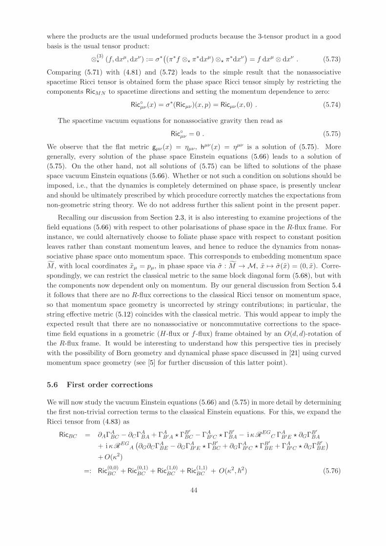
where the products are the usual undeformed products because the 3-tensor product in a good

basis is the usual tensor product:

⊗(3)⋆ (f,dxµ,dxν) := σ∗

((π∗f ⊗⋆ π

∗dxµ)⊗⋆ π∗dxν

)= f dxµ ⊗ dxν . (5.73)

Comparing (5.71) with (4.81) and (5.72) leads to the simple result that the nonassociative

spacetime Ricci tensor is obtained form the phase space Ricci tensor simply by restricting the

components RicMN to spacetime directions and setting the momentum dependence to zero:

Ricµν(x) = σ∗(Ricµν)(x, p) = Ricµν(x, 0) . (5.74)

The spacetime vacuum equations for nonassociative gravity then read as

Ricµν = 0 . (5.75)

We observe that the flat metric gµν(x) = ηµν , hµν(x) = ηµν is a solution of (5.75). More

generally, every solution of the phase space Einstein equations (5.66) leads to a solution of

(5.75). On the other hand, not all solutions of (5.75) can be lifted to solutions of the phase

space vacuum Einstein equations (5.66). Whether or not such a condition on solutions should be

imposed, i.e., that the dynamics is completely determined on phase space, is presently unclear

and should be ultimately prescribed by which procedure correctly matches the expectations from

non-geometric string theory. We do not address further this salient point in the present paper.

Recalling our discussion from Section 2.3, it is also interesting to examine projections of the

field equations (5.66) with respect to other polarisations of phase space in the R-flux frame. For

instance, we could alternatively choose to foliate phase space with respect to constant position

leaves rather than constant momentum leaves, and hence to reduce the dynamics from nonas-

sociative phase space onto momentum space. This corresponds to embedding momentum space

M , with local coordinates xµ = pµ, in phase space via σ : M → M, x 7→ σ(x) = (0, x). Corre-

spondingly, we can restrict the classical metric to the same block diagonal form (5.68), but with

the components now dependent only on momentum. By our general discussion from Section 5.4

it follows that there are no R-flux corrections to the classical Ricci tensor on momentum space,

so that momentum space geometry is uncorrected by stringy contributions; in particular, the

string effective metric (5.12) coincides with the classical metric. This would appear to imply the

expected result that there are no nonassociative or noncommutative corrections to the space-

time field equations in a geometric (H-flux or f -flux) frame obtained by an O(d, d)-rotation of

the R-flux frame. It would be interesting to understand how this perspective ties in precisely

with the possibility of Born geometry and dynamical phase space discussed in [21] using curved

momentum space geometry (see [5] for further discussion of this latter point).

5.6 First order corrections

We will now study the vacuum Einstein equations (5.66) and (5.75) in more detail by determining

the first non-trivial correction terms to the classical Einstein equations. For this, we expand the

Ricci tensor from (4.83) as

RicBC = ∂AΓABC − ∂CΓ

ABA + ΓAB′A ⋆ Γ

B′


BA − iκREG

C ΓAB′E ⋆ ∂GΓB′

BA

+ iκREG

A

(∂G∂CΓ

ABE − ∂GΓ

AB′E ⋆ Γ

B′

BC + ∂GΓAB′C ⋆ Γ

B′

BE + ΓAB′C ⋆ ∂GΓB′

BE

)

+O(κ2)

=: Ric(0,0)BC + Ric

(0,1)BC + Ric

(1,0)BC + Ric

(1,1)BC + O(κ2, ~2) (5.76)

44

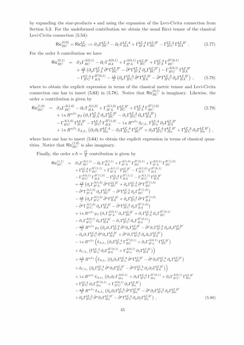
by expanding the star-products ⋆ and using the expansion of the Levi-Civita connection from

Section 5.3. For the undeformed contribution we obtain the usual Ricci tensor of the classical

Levi-Civita connection (5.54):

Ric(0,0)BC = RicLCBC := ∂AΓ

LCABC − ∂CΓ

LCABA + ΓLCA

B′A ΓLCB′

BC − ΓLCAB′C ΓLCB′

BA . (5.77)

For the order ~ contribution we have

Ric(0,1)BC = ∂AΓ

A(0,1)BC − ∂CΓ

A(0,1)BA + Γ

A(0,1)B′A ΓLCB′

BC + ΓLCAB′A Γ

B′(0,1)BC

+ i ~2

(∂µΓ

LCAB′A ∂µΓLCB′

BC − ∂µΓLCAB′A ∂µΓ

LCB′

BC

)− Γ

A(0,1)B′C ΓLCB′

BA

−ΓLCAB′C Γ

B′(0,1)BA − i ~

2

(∂µΓ

LCAB′C ∂µΓLCB′

BA − ∂µΓLCAB′C ∂µΓ

LCB′

BA

), (5.78)

where to obtain the explicit expression in terms of the classical metric tensor and Levi-Civita

connection one has to insert (5.63) in (5.78). Notice that Ric(0,1)BC is imaginary. Likewise, the

order κ contribution is given by

Ric(1,0)BC = ∂AΓ

A(1,0)BC − ∂CΓ

A(1,0)BA + Γ


BC + ΓLCAB′A Γ

B′(1,0)BC (5.79)

+ iκRαβγ pβ(∂γΓ

LCAB′A ∂αΓ

LCB′

BC − ∂γΓLCAB′C ∂αΓ

LCB′

BA

)

−ΓA(1,0)B′C ΓLCB′

BA − ΓLCAB′C Γ

B′(1,0)BA − i κRαβγ δC,xγ Γ

LCAB′α ∂βΓ

LCB′

BA

+ iκRαβγ δA,xγ(∂β∂CΓ

LCABα − ∂βΓ

LCAB′α ΓLCB′

BC + ∂βΓLCAB′C ΓLCB′

Bα + ΓLCAB′C ∂βΓ

LCB′

Bα

),

where here one has to insert (5.64) to obtain the explicit expression in terms of classical quan-

tities. Notice that Ric(1,0)BC is also imaginary.

Finally, the order κ~ = ℓ3s6 contribution is given by

Ric(1,1)BC = ∂AΓ

A(1,1)BC − ∂CΓ

A(1,1)BA + Γ

A(1,0)B′A Γ

B′(0,1)BC + Γ

A(0,1)B′A Γ

B′(1,0)BC

+ΓLCAB′A Γ

B′(1,1)BC + Γ


BC − ΓA(1,0)B′C Γ

B′(0,1)BA

−ΓA(0,1)B′C Γ

B′(1,0)BA − ΓLCA

B′C ΓB′(1,1)BA − Γ


BA

+ i ~2

(∂µΓ

A(1,0)B′A ∂µΓLCB′

BC + ∂µΓLCAB′A ∂µΓ

B′(1,0)BC

− ∂µΓA(1,0)B′A ∂µΓ

LCB′

BC − ∂µΓLCAB′A ∂µΓ

B′(1,0)BC

)

− i ~2

(∂µΓ

A(1,0)B′C ∂µΓLCB′

BA + ∂µΓLCAB′C ∂µΓ

B′(1,0)BA

− ∂µΓA(1,0)B′C ∂µΓ

LCB′

BA − ∂µΓLCAB′C ∂µΓ

B′(1,0)BA

)

+ iκRαβγ pβ(∂γΓ

A(0,1)B′A ∂αΓ

LCB′

BC + ∂γΓLCAB′A ∂αΓ

B′(0,1)BC

− ∂γΓA(0,1)B′C ∂αΓ

LCB′

BA − ∂γΓLCAB′C ∂αΓ

B′(0,1)BA

)

− κ ~

2 Rαβγ pβ(∂µ∂γΓ

LCAB′A ∂µ∂αΓ

LCB′

BC − ∂µ∂γΓLCAB′A ∂µ∂αΓ

LCB′

BC

− ∂µ∂γΓLCAB′C ∂µ∂αΓ

LCB′

BA + ∂µ∂γΓLCAB′C ∂µ∂αΓ

LCB′

BA

)

− iκRαβγ(δA,xγ

(∂βΓ

LCAB′α Γ

B′(0,1)BC + ∂βΓ

A(0,1)B′α ΓLCB′

BC

)

+ δC,xγ

(ΓLCAB′α ∂βΓ

B′(0,1)BA + Γ

A(0,1)B′α ∂βΓ

LCB′

BA

))

+ κ ~

2 Rαβγ(δA,xγ

(∂µ∂βΓ

LCAB′α ∂µΓLCB′

BC − ∂µ∂βΓLCAB′α ∂µΓ

LCB′

BC

)

+ δC,xγ

(∂µΓ

LCAB′α ∂µ∂βΓ

LCB′

BA − ∂µΓLCAB′α ∂µ∂βΓ

LCB′

BA

))

+ iκRαβγ δA,xγ

(∂β∂CΓ

A(0,1)Bα + ∂βΓ

LCAB′C Γ

B′(0,1)Bα + ∂βΓ


Bα

+ΓLCAB′C ∂βΓ

B′(0,1)Bα + Γ

A(0,1)B′C ∂βΓ

LCB′

Bα

)

− κ ~

2 Rαβγ δA,xγ

(∂µ∂βΓ

LCAB′C ∂µΓLCB′

Bα − ∂µ∂βΓLCAB′C ∂µΓ

LCB′

Bα

+ ∂µΓLCAB′C ∂µ∂βΓ

LCB′

Bα − ∂µΓLCAB′C ∂µ∂βΓ

LCB′

Bα

), (5.80)

45

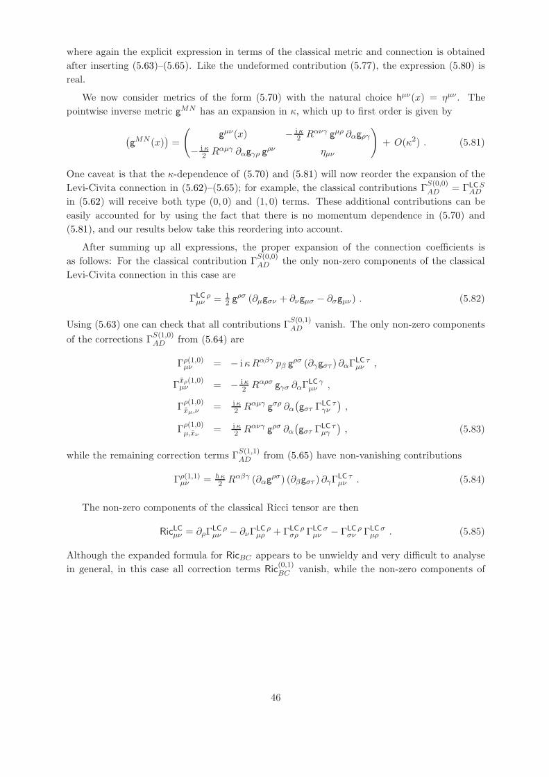
where again the explicit expression in terms of the classical metric and connection is obtained

after inserting (5.63)–(5.65). Like the undeformed contribution (5.77), the expression (5.80) is

real.

We now consider metrics of the form (5.70) with the natural choice hµν(x) = ηµν . The

pointwise inverse metric gMN has an expansion in κ, which up to first order is given by

(gMN (x)

)=

(gµν(x) − iκ

2 Rανγ gµρ ∂αgργ

− i κ2 Rαµγ ∂αgγρ g

ρν ηµν

)+ O(κ2) . (5.81)

One caveat is that the κ-dependence of (5.70) and (5.81) will now reorder the expansion of the

Levi-Civita connection in (5.62)–(5.65); for example, the classical contributions ΓS(0,0)AD = ΓLCS

AD

in (5.62) will receive both type (0, 0) and (1, 0) terms. These additional contributions can be

easily accounted for by using the fact that there is no momentum dependence in (5.70) and

(5.81), and our results below take this reordering into account.

After summing up all expressions, the proper expansion of the connection coefficients is

as follows: For the classical contribution ΓS(0,0)AD the only non-zero components of the classical

Levi-Civita connection in this case are

ΓLC ρµν = 1

2 gρσ (∂µgσν + ∂νgµσ − ∂σgµν) . (5.82)

Using (5.63) one can check that all contributions ΓS(0,1)AD vanish. The only non-zero components

of the corrections ΓS(1,0)AD from (5.64) are

Γρ(1,0)µν = − iκRαβγ pβ gρσ (∂γgστ ) ∂αΓ

LC τµν ,

Γxρ(1,0)µν = − iκ

2 Rαρσ gγσ ∂αΓLC γµν ,

Γρ(1,0)xµ,ν

= iκ2 Rαµγ gσρ ∂α

(gστ Γ

LC τγν

),

Γρ(1,0)µ,xν

= iκ2 Rανγ gρσ ∂α

(gστ Γ

LC τµγ

), (5.83)

while the remaining correction terms ΓS(1,1)AD from (5.65) have non-vanishing contributions

Γρ(1,1)µν = ~κ2 Rαβγ (∂αg

ρσ) (∂βgστ ) ∂γΓLC τµν . (5.84)

The non-zero components of the classical Ricci tensor are then

RicLCµν = ∂ρΓLC ρµν − ∂νΓ

LC ρµρ + ΓLC ρ

σρ ΓLCσµν − ΓLC ρ

σν ΓLCσµρ . (5.85)

Although the expanded formula for RicBC appears to be unwieldy and very difficult to analyse

in general, in this case all correction terms Ric(0,1)BC vanish, while the non-zero components of

46

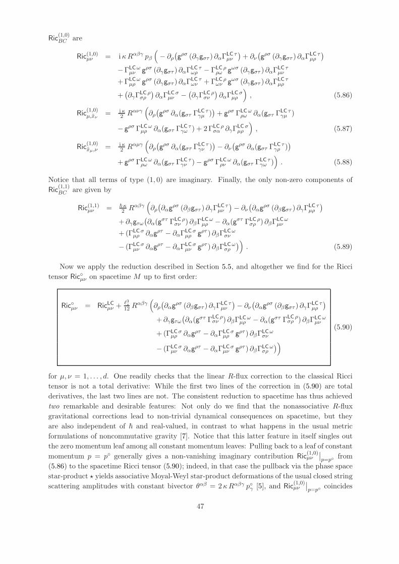
Ric(1,0)BC are

Ric(1,0)µν = iκRαβγ pβ

(− ∂ρ

(gρσ (∂γgστ ) ∂αΓ

LC τµν

)+ ∂ν

(gρσ (∂γgστ ) ∂αΓ

LC τµρ

)

−ΓLCωµν gρσ (∂γgστ ) ∂αΓ

LC τωρ − ΓLC ρ

ρω gωσ (∂γgστ ) ∂αΓLC τµν

+ΓLCωµρ gρσ (∂γgστ ) ∂αΓ

LC των + ΓLC ρ

ων gωσ (∂γgστ ) ∂αΓLC τµρ

+(∂γΓ

LC ρσρ

)∂αΓ

LCσµν −

(∂γΓ

LC ρσν

)∂αΓ

LCσµρ

), (5.86)

Ric(1,0)µ,xν

= i κ2 Rανγ

(∂ρ(gρσ ∂α(gστ Γ

LC τγµ )

)+ gρσ ΓLCω

ρω ∂α(gστ ΓLC τγµ )

− gρσ ΓLCωµρ ∂α(gστ Γ

LC τγω ) + 2ΓLC ρ

σα ∂γΓLCσµρ

), (5.87)

Ric(1,0)xµ,ν

= i κ2 Rαµγ

(∂ρ(gρσ ∂α(gστ Γ

LC τγν )

)− ∂ν

(gρσ ∂α(gστ Γ

LC τγρ )

)

+ gρσ ΓLCωρω ∂α(gστ Γ

LC τγν )− gρσ ΓLCω

ρν ∂α(gστ ΓLC τγω )

). (5.88)

Notice that all terms of type (1, 0) are imaginary. Finally, the only non-zero components of

Ric(1,1)BC are given by

Ric(1,1)µν = ~κ2 Rαβγ

(∂ρ(∂αg


)− ∂ν

(∂αg


)





LCωµν

+(ΓLCσµρ ∂αg


LCωσν



LCωσρ

)). (5.89)

Now we apply the reduction described in Section 5.5, and altogether we find for the Ricci

tensor Ricµν on spacetime M up to first order:

Ricµν = RicLCµν +ℓ3s12 R

αβγ(∂ρ(∂αg


)− ∂ν

(∂αg


)





LCωµν

+(ΓLCσµρ ∂αg


LCωσν



LCωσρ

))(5.90)

for µ, ν = 1, . . . , d. One readily checks that the linear R-flux correction to the classical Ricci

tensor is not a total derivative: While the first two lines of the correction in (5.90) are total

derivatives, the last two lines are not. The consistent reduction to spacetime has thus achieved

two remarkable and desirable features: Not only do we find that the nonassociative R-flux

gravitational corrections lead to non-trivial dynamical consequences on spacetime, but they

are also independent of ~ and real-valued, in contrast to what happens in the usual metric

formulations of noncommutative gravity [7]. Notice that this latter feature in itself singles out

the zero momentum leaf among all constant momentum leaves: Pulling back to a leaf of constant

momentum p = p generally gives a non-vanishing imaginary contribution Ric(1,0)µν

∣∣p=p

from

(5.86) to the spacetime Ricci tensor (5.90); indeed, in that case the pullback via the phase space

star-product ⋆ yields associative Moyal-Weyl star-product deformations of the usual closed string

scattering amplitudes with constant bivector θαβ = 2κRαβγ pγ [5], and Ric(1,0)µν

∣∣p=p

coincides

47

with the first order contribution to the noncommutative Ricci tensor from [7]. The potential

physical significance of the p 6= 0 leaves is discussed in [5].

It would be interesting to confirm explicitly that these features all persist to higher orders,

and to find explicit solutions of the spacetime vacuum equations (5.75) for nonassociative grav-

ity. Note that these equations are linear in the R-flux, whereas the H-flux modified Einstein

equations at leading order in string worldsheet perturbation theory and for constant dilaton

read RicLCµν = 14 Hµαβ Hν

αβ which by T-duality would naively imply that the leading correc-

tions should be of quadratic order in the R-flux. Here the first non-trivial contribution to the

spacetime curvature tensor is of order O(κ~) which is the order in which the first nonassociative

contributions appear. As this is a second order contribution when one expands the twist element

(2.3), it is natural that the curvature (and torsion) have corrections at this order.

6 Conclusions

In this paper we have provided and developed a formalism leading to a consistent approach to

nonassociative gravity induced by locally non-geometric constant R-flux backgrounds of string

theory in the parabolic phase space model of [25]. The construction relied on the proper char-

acterization of tensor fields in nonassociative geometry as well as their covariance under the

quasi-Hopf algebra generated by infinitesimal diffeomorphisms on twisted nonassociative phase

space. The unique Levi-Civita connection of any metric g has been determined at all orders in

the nonassociative deformation parameters. The vacuum Einstein equations have been obtained

also at all orders, and the first order corrections to the classical equations explicitly calculated,

which is the order at which the corresponding string theory calculations are reliable.

We have then pulled back the vacuum Einstein equations on phase space M to spacetime

M via the zero momentum section σ :M → M. General covariance of these latter equations is

on the one hand guaranteed by the geometric pullback operation. On the other hand, it could

be studied explicitly by considering the projection of the quantum Lie algebra of nonassociative

diffeomorphisms from Section 3.7 to the zero momentum leaf, as pursued in [5], where it was

illustrated how nonassociativity survives in the action of diffeomorphisms on spacetime. Ul-

timately, these symmetries should be compared to the classical diffeomorphism symmetries of

closed string theory and to the generalised diffeomorphism symmetries of double field theory.

Further insights into this nonassociative theory of gravity on spacetime should be obtained

by studying the pullbacks to spacetime also of the torsion and the Riemann curvature tensors.

Additional investigations relating the curved phase space geometry to the curved spacetime

geometry, and in particular the other possible spacetime geometries obtained by considering

different foliations of the manifold M, and not only those defined by constant momentum leaves

and constant position leaves, are left for future work. These investigations, and the construction

of a dynamical action principle for nonassociative gravity, should clarify the expected relevance

in the contexts of closed string theory and double field theory of the field equations we have

obtained, and in particular their interpretations as low-energy effective field equations of closed

string theory.

48

Acknowledgments

We thank Ralph Blumenhagen, Leonardo Castellani, Michael Fuchs, Chris Hull, Dieter Lust,

Emanuel Malek, Eric Plauschinn, Alexander Schenkel and Peter Schupp for helpful discussions.

This work was supported in part by the Action MP1405 QSPACE from the European Coopera-

tion in Science and Technology (COST). The work of P.A. and R.J.S. was supported in part by

the Research Support Fund of the Edinburgh Mathematical Society, and by the Consolidated

Grant ST/L000334/1 from the UK Science and Technology Facilities Council. The work of P.A.

is partially supported by INFN, CSN4, Iniziativa Specifica GSS. P.A. is also affiliated to INdAM,

GNFM (Istituto Nazionale di Alta Matematica, Gruppo Nazionale di Fisica Matematica). The

work of M.D.C. is supported by Project ON171031 of the Serbian Ministry of Education and

Science.

References

[1] D. Andriot, M. Larfors, D. Lust and P. Patalong, “(Non)commutative closed string onT-dual toroidal backgrounds,” JHEP 1306 (2013) 021 [arXiv:1211.6437 [hep-th]].

[2] P. Aschieri, “Noncommutative Riemannian geometry and gravity”, in preparation.

[3] P. Aschieri and L. Castellani, “Noncommutative gravity solutions,” J. Geom. Phys. 60(2010) 375–393 [arXiv:0906.2774 [hep-th]].

[4] P. Aschieri and A. Schenkel, “Noncommutative connections on bimodules and Drinfeld twistdeformation,” Adv. Theor. Math. Phys. 18 (2014) 513–612 [arXiv:1210.0241 [math.QA]].

[5] P. Aschieri and R.J. Szabo, “Triproducts, nonassociative star-products and geometry ofR-flux string compactifications,” J. Phys. Conf. Ser. 634 (2015) 012004 [arXiv:1504.03915[hep-th]].

[6] P. Aschieri, M. Dimitrijevic, F. Meyer and J. Wess, “Noncommutative geometry and grav-ity,” Class. Quant. Grav. 23 (2006) 1883–1912 [arXiv:hep-th/0510059].

[7] P. Aschieri, C. Blohmann, M. Dimitrijevic, F. Meyer, P. Schupp and J. Wess, “Agravity theory on noncommutative spaces,” Class. Quant. Grav. 22 (2005) 3511–3532[arXiv:hep-th/0504183].

[8] I. Bakas and D. Lust, “3-cocycles, nonassociative star-products and the magnetic paradigmof R-flux string vacua,” JHEP 1401 (2014) 171 [arXiv:1309.3172 [hep-th]].

[9] I. Bakas and D. Lust, “T-duality, quotients and currents for non-geometric closed strings,”Fortsch. Phys. 63 (2015) 543–570 [arXiv:1505.04004 [hep-th]].

[10] G.E. Barnes, A. Schenkel and R.J. Szabo, “Nonassociative geometry in quasi-Hopf repre-sentation categories I: Bimodules and their internal homomorphisms,” J. Geom. Phys. 89(2015) 111–152 [arXiv:1409.6331 [math.QA]].

[11] G.E. Barnes, A. Schenkel and R.J. Szabo, “Nonassociative geometry in quasi-Hopf repre-sentation categories II: Connections and curvature,” J. Geom. Phys. 106 (2016) 234–255[arXiv:1507.02792 [math.QA]].

[12] G.E. Barnes, A. Schenkel and R.J. Szabo, “Working with nonassociative geometry and fieldtheory,” PoS CORFU 2015 (2016) 081 [arXiv:1601.07353 [hep-th]].

[13] C.D.A. Blair, “Noncommutativity and nonassociativity of the doubled string in non-geometric backgrounds,” JHEP 1506 (2015) 091 [arXiv:1405.2283 [hep-th]].

49

http://arxiv.org/abs/1211.6437




http://arxiv.org/abs/hep-th/0510059

http://arxiv.org/abs/hep-th/0504183







[14] R. Blumenhagen and M. Fuchs, “Towards a theory of nonassociative gravity,” JHEP 1607(2016) 019 [arXiv:1604.03253 [hep-th]].

[15] R. Blumenhagen and E. Plauschinn, “Nonassociative gravity in string theory?,” J. Phys. A44 (2011) 015401 [arXiv:1010.1263 [hep-th]].

[16] R. Blumenhagen, A. Deser, D. Lust, E. Plauschinn and F. Rennecke, “Non-geometricfluxes, asymmetric strings and nonassociative geometry,” J. Phys. A 44 (2011) 385401[arXiv:1106.0316 [hep-th]].

[17] R. Blumenhagen, M. Fuchs, F. Hassler, D. Lust and R. Sun, “Nonassociative deformationsof geometry in double field theory,” JHEP 1404 (2014) 141 [arXiv:1312.0719 [hep-th]].

[18] M. Bojowald, S. Brahma, U. Buyukcam and T. Strobl, “Monopole star-products are non-alternative,” JHEP 1704 (2017) 028 [arXiv:1610.08359 [math-ph]].

[19] C. Condeescu, I. Florakis and D. Lust, “Asymmetric orbifolds, non-geometric fluxes andnoncommutativity in closed string theory,” JHEP 1204 (2012) 121 [arXiv:1202.6366 [hep-th]].

[20] V.G. Drinfeld, “Quasi-Hopf algebras,” Alg. Anal. 1N6 (1989) 114–148.

[21] L. Freidel, R.G. Leigh and D. Minic, “Born reciprocity in string theory and the nature ofspacetime,” Phys. Lett. B 730 (2014) 302–306 [arXiv:1307.7080 [hep-th]].

[22] C. Kassel, Quantum Groups (Springer, New York, 1995).

[23] V.G. Kupriyanov and R.J. Szabo, “G2-structures and quantization of non-geometric M-theory backgrounds,” JHEP 1702 (2017) 099 [arXiv:1701.02574 [hep-th]].

[24] V.G. Kupriyanov and D.V. Vassilevich, “Nonassociative Weyl star-products,” JHEP 1509(2015) 103 [arXiv:1506.02329 [hep-th]].

[25] D. Lust, “T-duality and closed string noncommutative (doubled) geometry,” JHEP 1012(2010) 084 [arXiv:1010.1361 [hep-th]].

[26] D. Mylonas, P. Schupp and R.J. Szabo, “Membrane sigma-models and quantization ofnon-geometric flux backgrounds,” JHEP 1209 (2012) 012 [arXiv:1207.0926 [hep-th]].

[27] D. Mylonas, P. Schupp and R.J. Szabo, “Non-geometric fluxes, quasi-Hopf twist de-formations and nonassociative quantum mechanics,” J. Math. Phys. 55 (2014) 122301[arXiv:1312.1621 [hep-th]].

[28] R.D. Schafer, An Introduction to Nonassociative Algebras (Dover Publications, New York,1995).

50













dipartimento di scienze e innovazione tecnologica ... · colin maclaurin building, riccarton,...

Documents