diplomarbeit - elib.dlr.de · diplomarbeit (theoretisch) von cand. ing. patrick hubert wagner...
TRANSCRIPT

Diplomarbeit (Theoretisch)
von cand. Ing. Patrick Hubert Wagner
Thermodynamic simulation of solar thermal
power stations with liquid salt as heat transfer
fluid
Betreuer: Dipl.-Ing. Christoph Wieland
Ausgegeben: 01.04.2012
Abgegeben: 28.09.2012
Prof. Dr.-Ing. Hartmut Spliethoff


Eidesstattliche Erklärung
Hiermit versichere ich, die vorliegende Arbeit selbständig und ohne Hilfe Dritter
angefertigt zu haben. Gedanken und Zitate, die ich aus fremden Quellen direkt
oder indirekt übernommen habe sind als solche kenntlich gemacht. Diese Arbeit
hat in gleicher oder ähnlicher Form noch keiner Prüfungsbehörde vorgelegen und
wurde bisher nicht veröffentlicht.
Ich erkläre mich damit einverstanden, dass die Arbeit durch den Lehrstuhl für
Energiesysteme der Öffentlichkeit zugänglich gemacht werden kann.
_________, den ___________ _______________________
Unterschrift


I
Abstract
This thesis was written at the Deutsches Zentrum für Luft- und Raumfahrt e. V.
(German Aerospace Center) in the Institute of Solar Research, Stuttgart. The
adviser was Dr.-Ing. Michael Wittmann from the Line Focus Systems division.
The Gemasolar solar power tower plant uses molten salt as heat transfer fluid and
is therefore the first commercial project to apply this technology. Current research
and development in line focusing systems is concentrated on transferring this
proved salt technology to solar thermal power stations with parabolic trough
collectors.
This thesis identifies the economic performance of such a power station. To that
end, a transient thermodynamic model is implemented into the commercial
software tool EBSILON®Professional. The system behavior of the solar field is
modelled in transient and pseudo-transient mode for the power block.
The model discretized one year into 10-minute intervals in order to calculate the
levelized electric costs (LECs) for a 125-MWe reference plant with live steam
parameters of 150 bar and 510 °C. The solar field layout is assumed to be a
2 H layout with 352 collector loops, each consisting of four Eurotrough ET150
collectors (solar multiple of 2.233). The storage system is able to feed the steam
generator for 10 hours.
Three different years with different annual averaged direct normal irradiation
averaged annual sums were compared. Given the 90% confidence interval
(50% ± 45%), the LECs are between 0.117 and 0.190 €/kWhe (2659 kWh/m²/y),
0.136 and 0.221 €/kWhe (2300 kWh/m²/y), and 0.149 and 0.243 €/kWhe
(2095 kWh/m²/y). The mode LECs are 0.149 €/kWhe, 0.172 €/kWhe, and
0.190 €/kWhe.
Key Words: Solar thermal power station, parabolic trough collector, molten salt,
annual yield calculation

II

Table of contents III
Table of contents
1 Introduction ................................................................................................. 1
2 State of the art ............................................................................................. 5
2.1 Configuration of a solar power plant with parabolic trough collectors and
molten salt as heat transfer fluid ....................................................................... 5
2.2 Parabolic trough collectors ..................................................................... 6
2.3 Parabolic trough receivers ..................................................................... 9
2.4 Heat transfer fluids in solar power stations with parabolic trough
collectors ........................................................................................................... 11
2.5 Advantages and disadvantages of using molten salt as heat transfer fluid
in parabolic trough solar power plants .............................................................. 16
2.6 Current projects...................................................................................... 18
2.6.1 ENEA research and development activities .................................... 18
2.6.1.1 Prova Collettori Solari .................................................................. 18
2.6.1.2 Archimede solar thermal power plant .......................................... 19
2.6.2 DLR research and development activities ....................................... 21
3 Modelling of the solar thermal power plant .............................................. 22
3.1 Solar field ............................................................................................... 23
3.1.1 Heat transfer fluid ............................................................................ 25
3.1.2 The sun ........................................................................................... 26
3.1.3 Solar field layout ............................................................................. 27
3.1.4 Parabolic trough collector ............................................................... 30

IV Table of contents
3.1.5 Pipings and headers ....................................................................... 34
3.1.6 Solar thermal storage system.......................................................... 37
3.1.7 Auxiliary heater ............................................................................... 39
3.1.8 Transient behavior of the solar field ................................................ 40
3.1.8.1 Collector ...................................................................................... 43
3.1.8.2 Header ......................................................................................... 44
3.1.8.3 Feeders 1 and 2 .......................................................................... 46
3.2 Power block ............................................................................................ 47
3.2.1 Steam generator ............................................................................. 49
3.2.2 Steam turbine .................................................................................. 52
3.2.3 Condenser and cooling system ....................................................... 53
3.2.4 Feed water heating ......................................................................... 54
3.2.5 Live steam extraction and off-design of the power block ................. 55
3.2.6 Pseudo-transient behavior of the power block ................................ 56
3.3 Plant operation management ................................................................. 58
3.4 Calculation procedure of the levelized electric costs .............................. 63
3.4.1 Economic model .............................................................................. 63
3.4.2 Statistical model .............................................................................. 65
4 Application of the solar thermal power station model ............................. 68
4.1 The reference plant ................................................................................ 68
4.1.1 Solar field ........................................................................................ 68
4.1.2 Power block..................................................................................... 69
4.2 Simulation of the reference plant ............................................................ 70
4.2.1 Numerical accuracy ......................................................................... 70

Table of contents V
4.2.2 Plant operation management .......................................................... 72
4.2.3 Results ............................................................................................ 74
4.3 Comparison of stationary and transient solar field model ....................... 76
4.4 Comparison of various time series time steps .................................... 80
4.5 Comparison of three years with different direct normal irradiation
averaged annual sum ................................................................................... 85
4.6 Improvement of the reference plant ................................................... 89
4.7 Comparison of various cooling methods ............................................ 92
5 Summary and Conclusion ...................................................................... 95
Appendix ......................................................................................................... 99
Appendix A: Screenshot of the Ebsilon model of the solar field .................... 99
Appendix B: Screenshot of the Ebsilon model of the power block .............. 100
Appendix C: User input parameters and output parameters for the design
process of the solar thermal power plant .................................................... 101
Appendix D: The time series dialog in Ebsilon ............................................ 106
Appendix E: Input and output parameters in the time series dialog ............ 107
Appendix F: Schematic of the EbsScript to design the power plant ............ 111
Appendix G: Schematic of the EbsScript for plant operation management,
executed before each time instant of the time series dialog ....................... 112
Appendix H: The parameters of the three implemented PTCs.................... 113
Appendix I: T-S diagram of the designed power block ................................ 114
Appendix J: Schematic of the profile selection implemented in EbsScript .. 115
Appendix K: Matlab Script for LEC calculation ............................................ 116
Appendix L: Parameters of the reference solar thermal power plant .......... 118

VI Table of contents
Appendix M: The location used for the simulation of the solar thermal power
plant ......................................................................................................... 123
Appendix N: Effect of the time discretization on the PTC efficiency ............ 127
Appendix O: Absolute value comparison of for 10-, 15-, 30-, and 60-minute time
series time step ........................................................................................... 131
Appendix P: Sankey diagrams of the Almería 2005, Almería 2010, and Las
Vegas 2008 improved simulation ................................................................ 132
Appendix Q: Ethical impact of steam turbine back-pressure in solar thermal
power plants ................................................................................................ 133
References ..................................................................................................... 135
Acknowledgment ............................................................................................ 143

List of figures VII
List of figures
Figure 1: Schematic configuration of a solar power plant with PTCs and molten
salt as HTF adapted from (Wittmann 2012) ......................................... 6
Figure 2: Schematic diagram of a parabolic trough collector (Flagsol 2012) ...... 7
Figure 3: Schematic diagram of a shortened parabolic trough receiver adapted
from (Mohr 1999, p. 9) ......................................................................... 9
Figure 4: Phase diagram of NaNO3-KNO3 (Kramer 1980) .............................. 13
Figure 5: Schematic of the Archimede solar power plant with PTC and molten
salt as HTF (Falchetta 2010) ............................................................. 20
Figure 6: Model of the solar field with Ebsilon .................................................. 24
Figure 7: The angles of a parabolic trough collector and of the sun adopted
from (Schenk 2012, p. 21) ................................................................. 26
Figure 8: Schematic of one quarter of the I layout, H layout, 3/2 H layout and
2 H layout with labelled characteristic components ........................... 27
Figure 9: Scheme of the PTC focus control ...................................................... 32
Figure 10: Heat losses of the Schott PTR 70 receiver tested at NREL –
uncertainty of W/m is shown ..................................................... 33
Figure 11: Geometry of the headers and feeders used in the Ebsilon model of
the solar thermal power plant ............................................................ 35
Figure 12: Heat losses of piping elements tested by ENEA adopted from
(Maccari 2006) ................................................................................... 36
Figure 13: Model of the auxiliary heater in Ebsilon ........................................... 39
Figure 14: The geometry of the indirect storage element, component 119,
adapted from (Pulyaev 2011, p. 23) .................................................. 41
Figure 15: Simulated start-up process of the solar field with solar salt as HTF
from minimum temperature of 270 °C to operating temperature of
510 °C on June 20, 2008 in Las Vegas ............................................. 44

VIII List of figures
Figure 16: Schematic of the distributing header with a specific number of
branches adapted from (Hirsch 2010) ............................................... 45
Figure 17: Model of the power block with Ebsilon ............................................. 48
Figure 18: Q,T diagram of a steam generator at the design point for a
125-MWe power plant with solar salt at 510 °C as HTF ..................... 50
Figure 19: Shell and tube heat exchanger adapted from (VDI 2006, p. Cc1) ... 50
Figure 20: Q,T diagram of the feed water heating at the design point for a
125-MWe power plant with solar salt at 510 °C as HTF – AC6, PH6
are not active ..................................................................................... 54
Figure 21: Off-design behavior for a 125-MWe power plant with solar salt at
510 °C as HTF ................................................................................... 55
Figure 22: Simulated start-up procedure of the power block from 30% load
(37.5 MWe) to 100% load (125 MWe) in ten-minute resolution in Las
Vegas on January 1, 2008 ................................................................. 58
Figure 23: Schematic of the simulation mode selection implemented in Ebsilon61
Figure 24: Schematic of the economic model to calculate the levelized electric
costs .................................................................................................. 64
Figure 25: Classification of 2008 in Las Vegas in a) weather conditions and b)
selected profiles ................................................................................. 73
Figure 26: Sankey diagram of the reference plant ............................................ 75
Figure 27: Annual energy comparison for stationary and transient simulation –
transient simulation refers to 100% .................................................... 78
Figure 28: Comparison of stationary and transient simulation on October 3,
2008 in Las Vegas ............................................................................. 78
Figure 29: DNI discretization comparison for three different TSs in Las Vegas
on January 1, 2008 ............................................................................ 81
Figure 30: Maximum 60- and 30-minute discretization error due to less
collected solar energy than the original 1-minute data, during a
summer day ....................................................................................... 82

List of figures IX
Figure 31: Annual energy comparison for 10-, 15-, 30-, and 60-minute TS –
100% is 10-minute TS ....................................................................... 84
Figure 32: The a) probability density function and b) cumulative density
function of the LECs for Las Vegas 2008 (2659 kWh/m²/y), Almería
2005 (2300 kWh/m²/y) and 2010 (2095 kWh/m²/y), and the improved
PP of Las Vegas 2008 ....................................................................... 87
Figure 33: The LECs for Las Vegas 2008 (2659 kWh/m²/y), Almería 2005
(2300 kWh/m²/y) and 2010 (2095 kWh/m²/y), and the trend line of
direct normal irradiation averaged annual sum function to LECs ....... 89
Figure 34: Annual energy comparison for the reference and improved solar
thermal power plant – reference plant refers to 100% ....................... 91
Figure 35: PB efficiency to the PB load for two different cooling systems. ....... 93
Figure 36: The cumulative density function of the LECs for Las Vegas 2008
with wet cooling system, hybrid cooling system, and dry cooling
system ............................................................................................... 94
Figure 37: Worldwide annual direct normal irradiation in kWh/m²/y from NASA
SSE 6.0 adapted from (Trieb 2009) ................................................. 123
Figure 38: Annual direct normal irradiation for Almería from 2002 to 2011 and
Las Vegas from 2007 to 2011 .......................................................... 124
Figure 39: Temperature progress in Almería during 2010 .............................. 125
Figure 40: Temperature progress in Las Vegas during 2008 ......................... 125
Figure 41: Direct normal radiance progress in Almería during 2010 .............. 126
Figure 42: Direct normal radiance progress in Las Vegas during 2008 .......... 126
Figure 43: PTC efficiency a) over one year, and b) over three selected days
(21.06, 21.09, 21.12) ....................................................................... 127
Figure 44: CDF for the PTC efficiency integral over the day of December 21 –
efficiency is discretized in 1-, 10-, 30-, and 60-minute resolution .... 129

X List of figures

List of tables XI
List of tables
Table 1: Resource share in renewable energy sources for electricity (RES-E)
production for the EU-27 and the Middle East and North Africa
(MENA) region for the years 2010, 2020, and 2050 ............................ 2
Table 2: Main characteristic parameters of EuroTrough ET150, HelioTrough,
UltimateTrough, and Ronda RHT 2500 collectors ............................... 8
Table 3: Comparison of the main parameters of Archimede HEMS11, Schott
PTR 70, and PTR 80 parabolic trough receivers ............................... 10
Table 4: Characteristics of nitrate/nitrite salts and Therminol VP-1 .................. 12
Table 5: Characteristics of newly developed molten salts ................................ 15
Table 6: Design data of the Archimede Power Plant (Falchetta 2010) ............. 20
Table 7: The real components of a solar field and the modelled components in
Ebsilon ............................................................................................... 28
Table 8: Modelling of different solar field layouts .............................................. 29
Table 9: Pressure drops of the steam generator at the design point ................ 52
Table 10: The parameters of the steam turbine at the design point ................. 53
Table 11: Solar thermal power plant operation mode possibilities and the
implemented profiles (P) .................................................................... 59
Table 12: Changed parameters of the reference plant ..................................... 90
Table 13: Maximum, minimum, and average weather data for the year 2010 in
Almería and 2008 in Las Vegas ....................................................... 125

XII List of tables

Nomenclatur XIII
Nomenclatur
AH Auxiliary heater
ASE Archimede Solar Energy
BMU Bundesministerium für Umwelt, Naturschutz und Reaktorsicherheit
BOP Balance of plant
cdf Cumulative density function
CSP Concentrating solar power
CT Cold tank
Dii Desertec Industrial Initative
DLR Deutsches Zentrum für Luft- und Raumfahrt
EBSILON Energy balance and simulation of the load response of power generating or process controlling network structures
Eco Economiser
ENEA National Agency for New Technologies, Energy and the Environment
ENEL Ente nazionale per l'energia elettrica
Eva Evaporator
FAME French Agency for the Management of Energy
HPS High Performance Solarthermie
HT Hot tank
HTF Heat transfer fluid
IAM Incident angle modifier
LEC Levelized electric cost

XIV Nomenclatur
MENA Middle East and North Africa
MM Mass multiplier
NREAP Renewable Energy Projections as Published in the National Renewable Energy Action Plans of the European Member States
NREL National Renewable Energy Laboratory
P Profile
PB Power block
PCS Prova collettori solari
pdf Probability density function
PP Power plant
PTC Parabolic trough collector
PTR Parabolic trough receiver
PV Photovoltaic
RES-E Renewable energy sources for electricity
RH Reheater
SCA Solar collector assembly
SCE Solar collector elements
SEGS Solar electric generation system
SF Solar field
SG Steam generator
SH Superheater
TS Time series time step

Nomenclatur XV
Subscripts
Abs Absorber
amb ambient
Ape Aperture
b bending
br branch
clean cleanliness
D at the design point
dis discount
e electrical
em employee
end end losses
f focus
f1 feeder 1
f2 feeder 2
geo geometric
h header
hl heat losses
i inner
i incident
IS indirect storage
j numbering element
k numbering element

XVI Nomenclatur
l numbering element
off-D off-design
rep representative
rowdist row distance
s sun
shad shading
th thermal
u upper
w-s water-steam

Notation XVII
Notation
Notation Unit Meaning
[m²] area
[-] factor
[m²/s] thermal diffusivity
[-] geometric concentration
[J/kg/K] specific heat capacity
[-] capital recovery factor
[m] distance, diameter
[W/m²] direct normal irradiance
[-] exponent
[-] focus
( ) [-] cumulative density function
[€] cost for gas
[€] investment
[-] incident angle modifier
[€] cost for insurance
[-] correction factor
[W/m] specific heat loss
[m] length
[€/kWhe] levelized electric cost
[kg] mass

XVIII Notation
[kg/s] mass flow
[-] Nusselt number
[-] number
[€] cost for operation and maintenance
various specific cost
[Pa] pressure
[-] Prandtl number
( ) [-] probability density function
[J] energy
[W] heat flow
[J/m²] specific energy
[W/m²] specific heat flow
[kg/s/s] Ramp-up factor
[-] Reynolds number
[J/m³/K] volumetric heat capacity
[J/kg/K] entropy
[K] temperature
[s] time
[m] thickness
[W/m²/K] overall heat transfer coefficient
[m/s] velocity
[m] width

Notation XIX
Greek
[W/m²/K] heat transfer coefficient
[-] absorptance
[°] sun azimuth angle
[°] sun height angle
[-] intercept factor
[m] pipe wall roughness
[-] efficiency
[kg/m/s] dynamic viscosity
[°] angle (defined locally), angle between surface
normal and incident radiation
[W/m/K] heat conductivity
[-] mean
[-] friction force
[kg/m³] density
[-] reflectance
tracking angle of the parabolic trough collector
[-] standard deviation
[-] transmittance
[-] start-up state of the PB

XX Notation

1 Introduction 1
1 Introduction
On April 23, 2009, the European Parliament and the European Council released a
directive “on the promotion of the use of energy from renewable sources” which
states that the European Union’s goal is to generate 20% of its energy using
renewable energy sources by 2020. This includes energy for electricity, transport,
and heating and cooling (European Parliament 2009).
In order to reach that goal, the directive proposes an increase in electricity
production from renewables to approximately 34% (European Parliament 2007).
Table 1 shows the breakdown of the EU-27’s usage of renewable energy sources
for electricity (RES-E) production for 2010, which together amounted to 19.42% of
the total. Hydro power had the highest share, followed by wind, biomass, and solar
power, which is further divided into photovoltaic (PV) at 3.2% and concentrating
solar power (CSP) at 0.2%.
A clearer picture of the future development of RES-E may be obtained by
examining the following reports:
“Renewable Energy Projections as Published in the National Renewable
Energy Action Plans of the European Member States” (NREAP) by the
European Environment Agency (Beurskens 2011)
“Perspectives on a Sustainable Power System for EUMENA” by the
Desertec Industrial Initative (Dii) (Dii GmbH 2012)
The NREAP projects the situation of the EU-27 in the year 2020 based on a road
map to reach the 20% goal set by the EU. The Dii report examines a scenario in
2050 in which the EU-27 imports 19% of its total electricity consumption from the
Middle East and North Africa (MENA) region. The NREAP report puts the
percentage of total electricity production from RES-E at 34.5%, while the Dii report
puts it at 92%. Table 1 shows the electricity production figures for 2020 contained
in the NREAP report: 495 TWh/y from wind power, 83 TWh/y from PV, and
20 TWh/y from CSP. The Dii report projects electric energy production in the
EU-27 and MENA regions in 2050 at 2678 TWh/y from wind power, 412 TWh/y
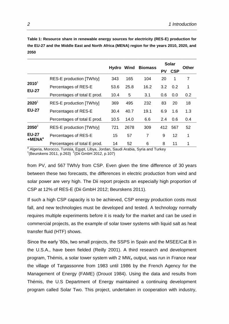
2 1 Introduction
from PV, and 567 TWh/y from CSP. Even given the time difference of 30 years
between these two forecasts, the differences in electric production from wind and
solar power are very high. The Dii report projects an especially high proportion of
CSP at 12% of RES-E (Dii GmbH 2012; Beurskens 2011).
If such a high CSP capacity is to be achieved, CSP energy production costs must
fall, and new technologies must be developed and tested. A technology normally
requires multiple experiments before it is ready for the market and can be used in
commercial projects, as the example of solar tower systems with liquid salt as heat
transfer fluid (HTF) shows.
Since the early ‘80s, two small projects, the SSPS in Spain and the MSEE/Cat B in
the U.S.A., have been fielded (Reilly 2001). A third research and development
program, Thémis, a solar tower system with 2 MWe output, was run in France near
the village of Targassonne from 1983 until 1986 by the French Agency for the
Management of Energy (FAME) (Drouot 1984). Using the data and results from
Thémis, the U.S Department of Energy maintained a continuing development
program called Solar Two. This project, undertaken in cooperation with industry,
Table 1: Resource share in renewable energy sources for electricity (RES-E) production for
the EU-27 and the Middle East and North Africa (MENA) region for the years 2010, 2020, and
2050
Hydro Wind Biomass Solar
Other PV CSP
20101
EU-27
RES-E production [TWh/y] 343 165 104 20 1 7
Percentages of RES-E 53.6 25.8 16.2 3.2 0.2 1
Percentages of total E prod. 10.4 5 3.1 0.6 0.0 0.2
20201
EU-27
RES-E production [TWh/y] 369 495 232 83 20 18
Percentages of RES-E 30.4 40.7 19.1 6.9 1.6 1.3
Percentages of total E prod. 10.5 14.0 6.6 2.4 0.6 0.4
20502
EU-27 +MENAa
RES-E production [TWh/y] 721 2678 309 412 567 52
Percentages of RES-E 15 57 7 9 12 1
Percentages of total E prod. 14 52 6 8 11 1 a Algeria, Morocco, Tunisia, Egypt, Libya, Jordan, Saudi Arabia, Syria and Turkey
1(Beurskens 2011, p.263)
2(Dii GmbH 2012, p.107)

1 Introduction 3
ran from June 1996 to April 1999. The solar power tower plant had an output of
10 MWe (Reilly 2001). Following the validation process for a new receiver design
for molten salt power towers at the Plataforma Solar de Almaría (PSA) in Spain
from 2006 to 2009, the Solar Two’s successor was built. Solar Trés, later called
Gemasolar, is the first commercial molten salt power tower with an output of
20 MWe. It supplied energy to the grid for the first time in May 2011. This project
was carried out by Torresol Energy in Fuentes de Andalucía, Spain (Burgaleta
2011).
At the moment, a major focus of research and development in solar power stations
is the transfer of proven molten salt technology from the tower system to other
types of collectors, e.g. parabolic dish, linear Fresnel, and parabolic trough
collectors (PTCs). Given the progress in PTC and absorber technology, a solar
power station with PTCs and molten salt as HTF seems to have good prospects.
This thesis optimises such a power station and outlines its economic potential.

4 1 Introduction

2 State of the art 5
2 State of the art
This chapter offers an overview of current technologies that are available on the
present market. It explains a solar thermal power station with PTC and salt as
HTF, examines the use of PTCs, receiver tubes, and molten salt as HTF in solar
technology, deduces the advantages and disadvantages of using molten salt as
HTF in PTC power plants, and provides an overview of current research and
development projects.
2.1 Configuration of a solar power plant with parabolic trough
collectors and molten salt as heat transfer fluid
Figure 1 shows the schematic configuration of a solar power plant with PTCs and
salt as HTF. The PP can be subdivided into four locally separated units: the
collector field, the back-up-system, the storage system, and the power block (PB).
These systems are connected by two closed loops: the molten salt circuit,
indicated by a green line, and the water steam circuit inside the PB.
If enough solar radiation is available, the molten salt from the cold tank is pumped
through the collector field, which consists of several loops with PTCs. The molten
salt is heated up to the design temperature and stored in the hot tank. The
back-up-system, an auxiliary heater connected parallel to the collector field, can
also heat the molten salt to the design temperature. If the hot tank is filled to its
minimum charging level, the production process can begin upon demand for
electricity: the molten salt is pumped through the steam generator (SG) in the PB,
exchanges its heat with the water steam circuit, and returns to the cold tank.
The PB is a conventional thermal power station like those used in fossil fuel power
stations. It is based on the Rankine cycle with reheat and steam extraction from
the turbine. The heat of the HTF is transferred via an SG to the water-steam cycle.
The thermal energy of the steam is converted into mechanical energy by the
steam turbine and finally to electric energy by the generator.

6 2 State of the art
2.2 Parabolic trough collectors
The collector field of the solar thermal power plant described in Chapter 2.1
consists of several PTCs, as shown in Figure 2. The parabolic reflector (1)
concentrates direct normal irradiation onto a linear absorber tube (2) located in the
focal line of the mirror. The geometric concentration, the ratio of aperture area
( ) to absorber area ( ),
(1)
of current collectors can be as high as 80. All current commercial mirrors are
second-surface silvered glass mirrors with a low fraction of iron oxide ( ),
which gives them very high transmittance, as their reflectivity is about 93 to 96 %
(Price 2002). Together, several mirrors along the vertical and horizontal axes form
one solar collector element (SCE), and several SCEs form one solar collector
assembly (SCA) with an aperture width of 4 to 6 m and a length of up to 150 m
Figure 1: Schematic configuration of a solar power plant with PTCs and molten salt as HTF
adapted from (Wittmann 2012)
Collector Field Storage-SystemBack-Up-System
Hot Tank
Cold Tank
Power
Block
Power Block
AuxiliaryHeater

2 State of the art 7
(Schenk 2012, p. 4). The collector tracks the sun in one dimension throughout the
day by means of a hydraulic drive and a local controller. The HTF is pumped
through the absorber tube and heated. Several collectors are serially connected
into one loop to reach high temperatures.
At the Solar Electric Generation System (SEGS) in the U.S.A., parabolic trough
system technology has been operated for more than 25 years, and its collectors
have improved constantly (Mohr 1999, p. 47). Drawing on the experience gained
during the LUZ LS-2 and LS-3 collector projects, the European consortium
EuroTrough built the ET100 and ET150 collectors. Table 2 lists the main
characteristic parameters of the ET150, which is made up of 12 SCEs, each
comprised of seven mirror panels along the horizontal axis and four in a vertical
cross-section. In all, one SCA contains 336 glass facets. At 18.5 kg per m², the
steel structure and pylons are 14 % lighter than the LS-3 collector, which means
that the solar field (SF) costs are also lower. However, there are fewer structural
deformations, which allows better optical performance in gusting wind. One loop
can be built with four to six SCAs producing HTF outlet temperatures of over
Figure 2: Schematic diagram of a parabolic trough collector (Flagsol 2012)

8 2 State of the art
500 °C. Solar plants equipped with ET150 PTCs can generate up to 200 MWe
(Geyer 2002).
After the testing of the EuroTrough collector in commercial PPs, e.g. Andasol I, II,
and III, successive generations of collectors were developed. Table 2 lists their
main parameters. The second generation, HelioTrough by Flagsol GmbH, has an
aperture width of 6.78 m, a module length of 19.1 m, fewer and longer SCEs, and
better optical performance. The third generation, UltimateTrough by
Flabeg GmbH, has an aperture width of 7.51 m, and its SCEs are twice as long as
the SCEs of the EuroTrough collector. It costs 25 % less than EuroTrough, and its
optical performance is 8 % better (Schweitzer 2011).
The Italian National Agency for New Technologies, Energy and the Environment
(ENEA) and the Ronda Group designed the RHT 2500 collector especially for the
Table 2: Main characteristic parameters of EuroTrough ET150, HelioTrough, UltimateTrough,
and Ronda RHT 2500 collectors
Property EuroTrough
ET1501 HelioTrough2 UltimateTrough2
Ronda
RHT 25003
Solar collector element (SCE)
Absorber diameter 0.07 m 0.09 m 0.09a m 0.07 m
Focal length 1.71 m 1.86a m 1.95a m 1.81 m
Aperture width 5.77 m 6.78 m 7.5 m 5.9 m
Length 12 m 19.1 m 24 m 12 m
Solar collector assembly (SCA)
Number of SCEs 12 10 10 n/a
Length 148.5 m 191 m 242 m n/a
Number of glass facets 336 480 480 n/a
Net aperture area 817.5 m² 1263 m² 1689 m² n/a
Optical parameters
Mirror reflectivity
( ) 94% 94a% 94a% 94%
a assumption
1(Geyer 2002)
2(Schweitzer 2011)
3(Falchetta 2009b)

2 State of the art 9
use of molten salt as HTF. Its geometric parameters are slightly larger than
EuroTrough’s (5.9 m aperture width, 1.81 m focal length, and 12 m module
length).
2.3 Parabolic trough receivers
Figure 3 shows a shortened view of a linear receiver for PTCs. The main feature is
the steel absorber tube with a special solar-selective surface. It has good
absorption in the solar spectrum range and low heat radiation emission. An
anti-reflective evacuated glass tube surrounding the absorber reduces convection
heat loss and protects the absorber from oxidation. A getter built inside the tube
maintains the vacuum. Because glass and metal expand at different rates, the
most sensitive part of the receiver is the glass-to-metal seal (Price 2002). Bellows
on the ends of the receiver tube solve this difficulty.
In the Andasol I, II, and III solar thermal power plants and many other commercial
projects, the Schott PTR 70 absorber is used, making this parabolic trough
receiver (PTR) state-of-the-art. Table 3 lists its technical details. The maximum
operating temperature of the steel pipe is 450 °C, making it unsuitable for use with
molten salt as HTF, which requires temperatures of over 500 °C. So far, only the
Italian company Archimede Solar Energy (ASE) has developed and tested an
Figure 3: Schematic diagram of a shortened parabolic trough receiver adapted from (Mohr
1999, p. 9)
10 2 State of the art
absorber for this field of application: the Archimede HEMS11. It is the “first
commercial salt receiver” (Martini 2010) for HTF at temperatures of up to 550 °C.
ASE has developed a special coating for the steel receiver in cooperation with
ENEA, which enables thermomechanical and thermochemical stability at
temperatures of up to 600 °C
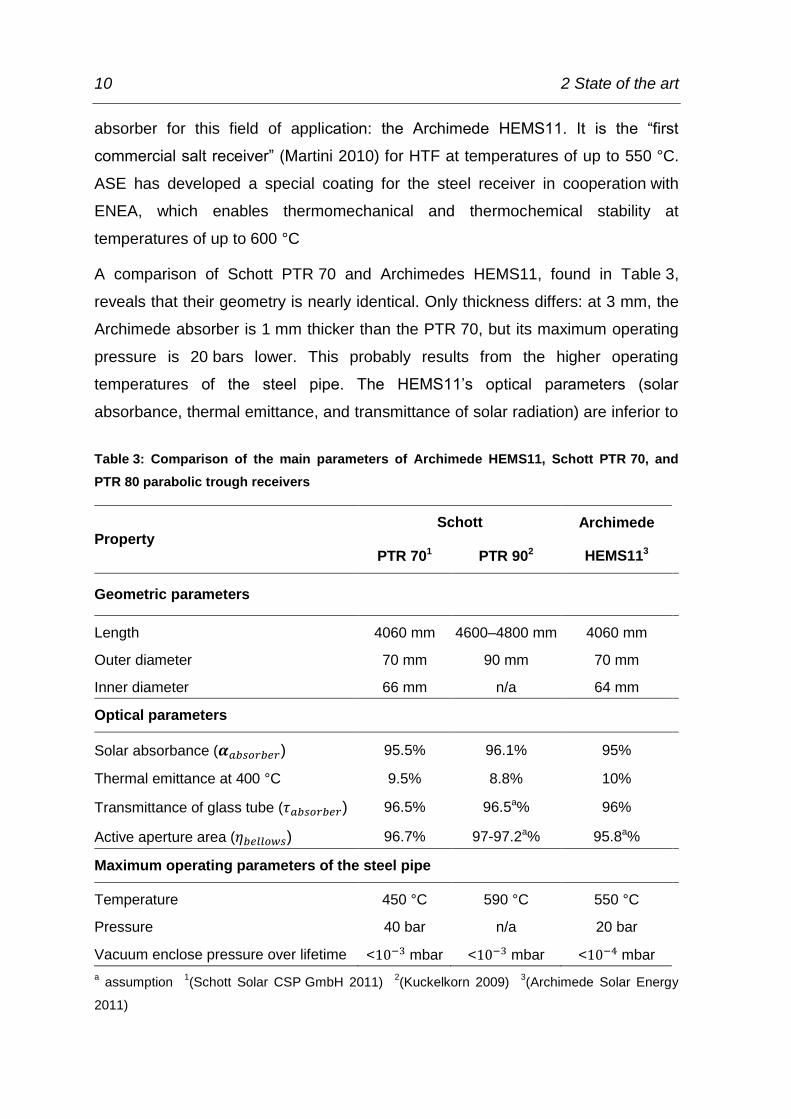
A comparison of Schott PTR 70 and Archimedes HEMS11, found in Table 3,
reveals that their geometry is nearly identical. Only thickness differs: at 3 mm, the
Archimede absorber is 1 mm thicker than the PTR 70, but its maximum operating
pressure is 20 bars lower. This probably results from the higher operating
temperatures of the steel pipe. The HEMS11’s optical parameters (solar
absorbance, thermal emittance, and transmittance of solar radiation) are inferior to
Table 3: Comparison of the main parameters of Archimede HEMS11, Schott PTR 70, and
PTR 80 parabolic trough receivers
Property Schott Archimede
HEMS113 PTR 701 PTR 902
Geometric parameters
Length 4060 mm 4600–4800 mm 4060 mm
Outer diameter 70 mm 90 mm 70 mm
Inner diameter 66 mm n/a 64 mm
Optical parameters
Solar absorbance ( ) 95.5% 96.1% 95%
Thermal emittance at 400 °C 9.5% 8.8% 10%
Transmittance of glass tube ( ) 96.5% 96.5a% 96%
Active aperture area ( ) 96.7% 97-97.2a% 95.8a%
Maximum operating parameters of the steel pipe
Temperature 450 °C 590 °C 550 °C
Pressure 40 bar n/a 20 bar
Vacuum enclose pressure over lifetime < mbar < mbar < mbar
a assumption
1(Schott Solar CSP GmbH 2011)
2(Kuckelkorn 2009)
3(Archimede Solar Energy
2011)

2 State of the art 11
the PTR 70’s, making its overall optical performance lower. This indicates that the
Schott absorber’s coating is slightly better. The PTR 70’s conductive heat losses
are marginally higher because its maximum vacuum enclose pressure over
lifetime is one order of magnitude higher.
To penetrate the next generation of the PTC solar power plant market, Schott
Solar is currently developing two new receiver designs, the PTR 80 and PTR 90.
Table 3 lists the parameters of the PTR 90 absorber. To compete with the
Archimede HEMS11 and employ molten salt as HTF, Schott developed a new
absorber coating which allows maximum operating temperatures of 590 °C. The
company also improved optical parameters, reduced heat losses by 20-30%, and
increased receiver length and diameter for use in the next generation of PTC, e.g.
the HelioTrough or UlimateTrough. The longer PTR increases the ratio of area of
bellows to active aperture area ( ), and the larger diameter increases the
fraction of the reflected sun rays incident upon the aperture that reach the PTR,
known as intercept factor ( ). These changes raise the optical efficiency
(2)
of the next PTC generation to 82%, 8% higher than the current design (Kuckelkorn
2009). The parameters of Eq. (2) are listed in Table 2 and Table 3.
2.4 Heat transfer fluids in solar power stations with parabolic
trough collectors
Table 4 lists commercially available HTFs for CSP power plants. The
state-of-the-art HTF for PTC power plants is a eutectic mixture of two very stable
compounds, biphenyl (C12H10) and diphenyl oxide (C12H10O). This organic
substance is sold by Solutia Inc. under the brand name Therminol VP-1 (Solutia
Inc 2012) and by Dow Chemical Company under the brand name Dowtherm A
(Dow Chemical Company 2001).
Therminol VP-1 is used for the SEGS in the U.S.A. Its advantages are its low
freezing point (12 °C) and low corrosion potential. But it also has several
disadvantages. It limits the SF’s maximum operating temperature to 400 °C due to
thermal degradation. Therminol VP-1 cannot be used as a thermal energy storage

12 2 State of the art
medium due to its high vapour pressure (approximately 10 bar at 390 °C), so an
indirect storage system, using thermal energy transfer to a second HTF, is needed
(Raade 2011b). This synthetic oil necessitates strict statutory requirements to
protect the local environment because it is toxic and at over 621 °C can
spontaneously combust (Solutia Inc. 2012). The commercially available organic
HTFs are also expensive (Mohr 1999, p. 74).
Table 4: Characteristics of nitrate/nitrite salts and Therminol VP-1
Property Solar Salt Hitec Hitec XL Therminol VP-1
Composition (weight percentage)
Salt1 NaNO3 60% 7% 15%
KNO3 40% 53% 43%
NaNO2 40%
Ca(NO3)2 42%
Organic
Compound 2
C12H10 73.5%
C12H10O 26.5%
Operating temperatures
Liquidus temperature [ °C] 2273 1415 1405 122,4
Upper temperature [ °C] 5934-6001 4545–5384 4605-5004,1 4002,4
Chemical properties at 400 °C6
Viscosity ( ) [mPas] 1.773 1.710 n/a 0.149
Heat conductivity ( )
[W/m/K]
0.511 0.330 n/a 0.076
Heat capacity ( ) [J/kg/K] 1516 1562 1304 2635
Density ( ) [kg/m³] 1834 1790 1903 694
Volumetric heat capacity ( )
[kJ/m³/K]
2780 2796 2482 1829
Economical parameters7
Nominal cost [$/kg] 0.49 0.93 1.19 2.2
1(Kelly 2007)
2(Solutia Inc 2012)
3(Kramer 1980)
4(Raade 2011b)
5(Bradshaw 1990)
6(Steag
2012) 7(Kearney 2003)

2 State of the art 13
A more promising HTF seems to be nitrate (NO3) and nitrite (NO2) salt mixtures.
These are used as HTF, as well as fluid for the storage tank, in the Gemasolar
commercial project (Burgaleta 2011) and in the Archimedes research project
(Falchetta 2010), which Chapter 2.6.1.2 describes in detail.
If a salt mixture is heated to its liquidus temperature, its cations and anions are
generally completely dissociated. Molten salts have high thermal stability, density,
and heat capacity, good thermal and electric conductivity, relatively low viscosity,
and a low vapour pressure, even at elevated temperatures (Baudis 2001, p. 5f).
Many varieties are available in large commercial quantities from several suppliers
(Raade 2011b). Table 4 shows the properties of three commercially available salt
mixtures sold by Solutia Incorporated: Solar Salt, Hitec, and Hitec XL. Solar salt is
a nearly eutectic binary mixture of potassium nitrate (KNO3) and sodium nitrate
(NaNO3), as shown in Figure 4. Hitec and Hitec XL are both eutectic ternary
mixtures of sodium nitrate, potassium nitrate, and sodium nitrite (NaNO2) (Hitec) or
calcium nitrate (Ca(NO3)2) (Hitec XL).
As Table 4 shows, a range of upper temperature limits for nitrate and nitrite salts is
given. At high temperatures, these salts undergo thermal decomposition, and the
insoluble products can plug pipes and valves, foul heat transfer surfaces, and
aggravate corrosion. Common impurities, such as water vapour or carbon
Figure 4: Phase diagram of NaNO3-KNO3 (Kramer 1980)
Solar Salt

14 2 State of the art
dioxides, affect the decomposition process. The upper temperature limit may also
be qualified when decomposition products are present or “a significant
concentration of decomposition products is reached” (Bradshaw 1990). All these
factors explain the variety of upper temperature limits for nitrate and nitrite salts
found in the literature.
Solar salt is the most stable salt in terms of thermal composition, usable at
temperatures of up to 600 °C under atmospheric conditions. It is also the cheapest
salt. But its liquidus temperature (227 °C) is very high. Hitec can be used at up to
454 °C under atmospheric conditions, the temperature at which thermal
decomposition starts, nitrite converts to nitrate, and Hitec’s freezing point rises
from 141 °C. If nitrogen gas is blanked to the salt, thermal decomposition begins at
538 °C (Kearney 2003). Hitec XL can be used at up to 500 °C under atmospheric
conditions.
New molten salts with a lower freezing temperature are currently under
development. Table 5 shows four non-commercial examples of recently developed
molten salt mixtures. Due to on-going testing, the chemical properties of these salt
mixtures are rarely available in literature. Despite their expanded temperature
range, the newly developed molten salts seem to have several problems, and
much remains unknown. The cost of the advanced HTF is higher than that of solar
salt. No chemical properties have been published so far (Raade 2011b). For
low-melting HTF, no long-term thermal stability analyses have been conducted.
The chlorides in the molten salt also tend to corrode steel alloys. Closer analyses
are pending (Raade 2011a). The TNS-4 has a density of 1,850 kg/m³ and a
dynamic viscosity of 1.8 mPas at 400 °C. These parameters are comparable to
those of solar salt. But the more critical parameter, specific heat capacity, has not
yet been published (Ren 2011). Sodium has also been proposed as an HTF. Its
density is 919 kg/m³, its specific heat capacity 1372 J/kg/K, its thermal conductivity
87 W/m/K, and its dynamic viscosity 0.008 mPas at 400 °C. In addition to its
greater temperature range, sodium’s low viscosity reduces pumping parasitics and
its very high thermal conductivity reduces the risk of hot spots. Its disadvantages
are its low volumetric heat capacity and its cost, which is 200% of Hitec’s. The
main problem with using sodium is that it is toxic and very flammable

2 State of the art 15
(Boerema 2012). The first solar tower project to use molten salt as HTF, the
SSPS, begun in 1981, used sodium. Its test facility was completely destroyed in a
sodium fire in 1986 (Reilly 2001). Sodium necessitates increased safety
precautions, which normally involve higher investment and operation cost.
Table 5: Characteristics of newly developed molten salts
Property Advanced
HTF1
Low-melting
HTF2
TNS-43 Liquid Sodium4
Composition (weight percentage)
Nitrate NaNO3 6% ?%
KNO3 23% 1% ?%
Ca(NO3)2 19%
CsNO3 44%
LiNO3 8% 21% ?%
Nitrite KNO2 45%
Ca(NO2)2 19%
NaNO2 12%
Other KCL 2%
Na 100%
Additive ?%
Operating temperatures
Liquidus temperature [ °C] 65 °C 53 °C 83 °C 97.9 °C
Upper temperature [ °C] 561 °C 481 °C 618 °C 873 °C
1(Raade 2011b)
2(Raade 2011a)
3(Ren 2011)
4(Boerema 2012)

16 2 State of the art
2.5 Advantages and disadvantages of using molten salt as heat
transfer fluid in parabolic trough solar power plants
There are several advantages to using molten salt instead of organic compounds
as HTF in PTC solar power plants. As explained in Chapter 2.4, the thermal
stability of molten salts allows higher temperatures – up to 600 °C, even at
atmospheric pressure – at the outlet of the SF. This results in higher temperatures
of live and reheat steam in the water-steam cycle, which improves the efficiency of
the Rankine cycle.
Molten salt HTF can also reduce the cost of thermal storage. Because of its low
price and good thermodynamic parameters, salt is widely used as a storage
medium. Its volumetric heat capacity is reasonable, and its vapour pressure is very
low, allowing storage under atmospheric pressure and eliminating the cost of thick
walls for the storage tank. It allows a direct storage system, unlike Therminol VP-1,
and so requires no additional heat exchangers, lowering investment costs and
increasing storage system efficiency because the system produces less entropy.
The temperature difference between the cold and the hot tanks – about 100 °C in
the current Andasol I solar power plant, for example (Relloso 2009) – is up to
300 °C with molten salt HTF. This and its higher volumetric heat capacity increase
the ratio of thermal storage capacity to storage tank volume.
Unlike Therminol VP-1, nitrate and nitrite salts are not toxic and have a high
autoignition temperature. Leakage will not harm the local environment, and the
danger of a fire is negligible (Benmarraze 2010).
The viscosity of the molten salt is twelve times that of Therminol VP-1. Pumping
the fluid through the piping elements would therefore normally require more power,
and SF parasitics would be higher. But “the mass flow in the solar field is
considerable [!] lower with molten salt, which leads to a lower pressure loss in the
piping. Both effects combined – low mass flow and low pressure loss – lead to
relatively low pumping parasitics compared to a (Therminol, editor’s note) VP-1
solar field” (Kearney 2002). Eq. (3) explains this effect. Given a constant heat flow
due to solar radiation to one PTC loop ( ), constant area of PTR ( ), and a

2 State of the art 17
constant HTF temperature rise through a PTC loop ( ), the only variable
parameter is the velocity of the HTF ( ) in the PTR.
(3)
Because the volumetric heat capacity ( ) of the molten salt is higher than that of
Therminol VP-1, the velocity is lower. Another reason is the higher when
using molten salt as HTF. These factors are more significant than the lower
viscosity.
Another advantage is flexible power plant management. Because molten salt is
used with a direct storage system, the SF and SG circuits are completely
decoupled. During periods of high radiation, thermal power is stored in the hot
tank. Upon demand for electric production, the hot molten salt supplies the SG
with thermal power and the plant produces electricity as long as the hot tank level
is high enough. Low storage system investment costs make a high storage
capacity economically viable, and a molten-salt-based solar power plant can
produce electricity even at night. 24-hour electricity production is possible, as
demonstrated at the Gemasolar power plant in May 2011 (Burgaleta 2011). Power
plant efficiency is also increased during the night because the ambient
temperature is lower. These effects make projectable electricity production
possible and increase the stability of electric power transmission. This is one of
CSP’s main advantages over other renewable energies such as photovoltaic or
wind energy.
Unfortunately, molten salt also has disadvantages. Table 4 shows the high
freezing point of nitrate and nitrite salts. The state-of-the-art nitrate salt, solar salt,
has a very high freezing point at 227 °C, which necessitates energy-intensive
freeze protection to avoid blockage of pipes and valves. This involves the
installation of additional hardware, e.g. impedance heating elements, heat tracing,
or insulation, which in turn entails high investment and operation costs (Kearney
2004).
Higher process temperatures also raise the average temperature of the SF,
causing higher radiation heat losses and lowering efficiency. Higher process
parameters also lead to pipe, valve, and pump corrosion. Common carbon steel’s

18 2 State of the art
corrosion rate is about 0.12 mm/y at process temperatures of up to 460 °C. At
higher temperatures, nickel-based alloys show a good corrosion rate – less than
1mm per century at temperatures of up to 600 °C. But they are also more
expensive than carbon steels (Bradshaw 1987).
2.6 Current projects
Presently, no commercial PTC power plant with molten salt as HTF is in operation.
However, two research and development programs run by ENEA and the German
Aerospace Center (DLR) are currently working with molten salt.
2.6.1 ENEA research and development activities
In 2001, ENEA released a strategy paper (ENEA 2007) that focuses, among other
things, on high-temperature (550 °C) heat production and storage. At this
temperature, a linear trough collector with molten salt as HTF is considered the
best solution. According to the paper, the following are to be achieved:
“A strong R&D programme in the few elements of parabolic trough” (ENEA
2007, p. 83)
“The realisation of a (…) demonstration power plant with parabolic troughs
(…) for a market niche in the 5 – 10 MWe production” (ENEA 2007, p. 83)
During the course of the research and development program, a PTC, the RHT
2500 collector, and a parabolic trough receiver (PTR), the Archimede HEMS08,
were invented. These collectors are discussed in Chapters 2.2 and 2.3.
2.6.1.1 Prova Collettori Solari
In 2004, the Prova Collettori Solari (PCS), a 100m PTC test circuit with solar salt
as HTF, began operation at ENEA Cassia Labs. Its goal was to test the PTC, PTR,
collector interconnectors, pumps, and heating system which had been developed
especially for molten salt usage. The test involved 1700 hours of operation and
about 160 SF filling and draining cycles, during which no critical situations arose or
accidents occurred. The draining and filling of the SF is the critical phase due to

2 State of the art 19
thermal losses and low salt mass flow – constant circulation of the salt can prevent
freezing even if temperature nears solidification. If the molten salt freezes, it
contracts, reducing its volume and causing no mechanical stress for piping
(Gaggioli 2007).
2.6.1.2 Archimede solar thermal power plant
After the successful PCS research and development period, ENEA and the Italian
electric utility company Ente nazionale per l'energia elettrica (ENEL) built the
Archimedes solar thermal power plant (5 MWe output) at Priolo Gargallo.
According to an ENEL press release (ENEL 2010), the Archimede Power Plant
was put into operation on July 14, 2010, and “is the first in the world (with PTC,
editor’s note), to use molten salts as the heat transfer fluid” (ENEL 2010). “Due to
the little size of the solar plant and the prototypal characteristics of its components,
the demonstration in [!] not fully representative with respect to economic viability of
the concept, but it is anyway a fundamental test of the technical aspects as
functionality, efficiency and reliability” (Crescenzi 2011).
Figure 5 shows a schematic of the power plant, and Table 6 lists Archimede’s
main design parameters. The SF consists of nine collector loops, each equipped
with six 100-meter-long PTCs. The solar salt is stored in a cold tank at 290 °C and
in a hot tank at 550 °C.
For the SF, there are three possible operating states (Falchetta 2009a):
Production: the HTF is pumped from the cold tank through the SF, heated
to 550 °C, and finally stored in the hot tank. The PTCs track the sun.
Re-circulation: the solar salt is pumped from the cold tank through SF and
the recirculation loop back to the cold tank. The PTCs track the sun. This
operating state occurs when there is insufficient solar radiation or during a
transient state, e.g. start-up in the morning or shut-down in the evening.
Night circulation: like re-circulation, but the collectors are in parked position,
oriented towards the ground.

20 2 State of the art
At nighttime, solar salt should be kept above 270 °C to prevent solidification of the
salt. To this end, additional electric heating elements are fitted to the pipes and the
two tanks. For the SG circuit, there are five possible operating states (Falchetta
2009a):
Table 6: Design data of the Archimede Power Plant (Falchetta 2010)
Solar field circuit
Number of collectors 54
Number of collector loops 9
Total collector surface 30580 m²
Annual direct normal irradiation 1936 kWh/m²/y
Storage size 80 MWth
Steam generator circuit
Steam generator capacity 12 MWth
Temperature of live steam 540 °C
Pressure of live steam 102 bar
Additional electric capacity 4.96 MWe
Figure 5: Schematic of the Archimede solar power plant with PTC and molten salt as HTF
(Falchetta 2010)

2 State of the art 21
Normal steam production
Steam production and heat restore to the cold tank
No steam production (standby)
No steam production and heat restore to the cold tank
Start-up
The SG is composed of three vertical heat exchangers: economizer, evaporator,
and superheater. It uses a steam drum with natural circulation. Live steam with a
pressure of 102 bar and a temperature of 540 °C is produced and fed into the
high-pressure stages of the combined-cycle power plant steam turbine (Falchetta
2009b).
Because two tanks are used, the SF circuit and SG circuit are completely
decoupled, allowing production of live steam when the SF is not in operation. The
hot tank capacity is sufficient for up to 6.6 hours.
2.6.2 DLR research and development activities
In a press release dated February 24, 2011 (Deutsches Zentrum für Luft- und
Raumfahrt 2011), the DLR announced that it would build a research and
development solar thermal power plant with PTCs and molten salt as HTF near
Evora, Portugal. This plan is supported by Bundesministerium für Umwelt,
Naturschutz und Reaktorsicherheit (BMU) within the framework of the High
Performance Solarthermie (HPS) joint research project. DLR’s project partners are
Siemens AG, K+S AG and Senior Flexonics GmbH. The project’s goal is to reach
temperatures above 500 °C with molten salt. To achieve this, the partners are
using the Siemens SunField 6 PTC, and the Archimede HEMS11 PTR by ASE.
The thermal energy of the molten salt is transferred in a newly developed
once-through boiler to the water-steam circuit. The project will also demonstrate
the economic feasibility and general plant safety of such technology. Solar salt is
to be used as HTF. During the joint research project, other salts with lower
freezing points are also to be investigated and their potentials identified
(Deutsches Zentrum für Luft- und Raumfahrt 2011; Siemens AG 2011).

22 3 Modelling of the solar thermal power plant
3 Modelling of the solar thermal power plant
The model of the solar thermal power plant with PTCs and molten salt as HTF is
created with the commercial simulation software EBSILON®Professional 10.01.01,
referred to as Ebsilon in this thesis, by Steag Energy Services GmbH. Ebsilon is
an abbreviation for “energy balance and simulation of the load response of power
generating or process controlling network structures”. It is a Windows-based
modelling tool with a graphical user interface that allows the drag-and-drop
arrangement of multiple pre-built components connected by material and logic
lines to simulate thermodynamic cycles.
The add-on EbsSolar, developed in cooperation with the DLR, offers components,
e.g line focusing collectors, thermal storages, headers, and distributers, to
simulate a solar thermal power plant. Besides the steady-state simulation both at
the design point and under off-design conditions, a successful model of an SF
requires transient simulation due the very dynamic environmental factors involved
in solar power plant operation. For this purpose, a time series calculation module,
an Excel-like spread-sheet, imports dynamic process variables, e.g. ambient
temperature and direct normal radiation, into the simulation model for different
time instants. Most components perform a steady simulation for each time instant.
Performing several consecutive steady simulations with the time series module
results in a quasi-instationary simulation. But there are also two fully transient
components: direct and indirect storage. The indirect storage is a simple pipe
model that calculates transient heat exchanges between the pipe and the fluid
flowing through it. The direct storage is a model of a transient storage tank that
can be charged or discharged between two time instants. It shows heat exchange
with the environment — cooling down or heating up. To track these two
components and the entire power plant over a series time instants, a Pascal-
based scripting language, EbsScript, is used.
EbsSolar and EbsScript allow the realistic simulation of the behavior of a solar
thermal power plant. The resulting simulation model is simple, fast, and
numerically robust enough to calculate annual yield based on transient system

3 Modelling of the solar thermal power plant 23
behavior. Appendix A contains a model of the solar field using PTCs and salt as
HTF, while Appendix B contains a model of the power block. The model creates
an interface for parameter input using the macro interface “Intelligence of power
plant”, shown as a blue box on the upper left border of the screenshot in
Appendix A. The interface allows several solar thermal power plant parameters
(listed in Appendix C) to be specified, generating an individual simulation model.
After parameter input, executing the EbsScript “Design power plant” results in the
design of specific parts of the power plant according to the input parameters.
Appendix F contains a schematic flow-chart of this script. The power plant design
process resulting parameters are listed in the lower rows of the table in
Appendix C. Following the solar thermal power plant design process, the time
series dialog shown in Appendix D allows annual yield calculations. The simulation
is performed by importing the ambient temperature and the direct normal radiation
for each time instant, represented by a row in the spreadsheet, into the simulation
model and entering the resulting parameters, listed in the table of Appendix E, into
the spreadsheet.
The following chapter describes in detail the simulation model of the solar field and
the power block. It examines the modelling of its components and the transient
system behavior more closely, and describes the model’s plant operation
management strategy based on the EbsScript schematically shown in Appendix G,
and the economic and statistical model to calculate the levelized electric cost
(LEC) in detail.
3.1 Solar field
The model of the solar field consists of the sun, the parabolic trough collectors
described in Chapter 2.2, distributing and collecting headers, feeders, two salt
submersion pumps, an auxiliary heater, and a cold and a hot storage tank.
Figure 6 contains a schematic drawing of the Ebsilon model.

24 3 Modelling of the solar thermal power plant
Fig
ure
6: M
od
el o
f the s
ola
r field
with
Eb
silo
n
Co
ld T
an
k
Ho
t Ta
nk
/
xx
Au
xilla
ry
He
ate
r
Po
we
r Blo
ck
Re
circ
ula
tion
loo
p
Co
mp
11
9: In
dire
ct s
tora
ge
(insta
tion
ary
)
Ph
oto
Ca
ptio
n
Co
mp
13: P
ipin
g (s
tatio
na
ry)
Co
mp
11
3: L
ine
focu
sin
g s
ola
r co
llecto
r
Co
mp
11
4 / 1
15
: Dis
tribu
ting
/ Co
llectin
g h
ea
de
r
xC
om
p 1
10
: Ma
ss m
ultip
lier
Co
mp
83: P
um
p (v
aria
ble
sp
ee
d)
Co
mp
11
8: D
irect s
tora
ge
/ ma
s s
tora
ge
(insta
tion
ary
)
Co
mp
4 / 7
: Sim
ple
sp
litter / S
imp
le m
ixe
r
Co
mp
3: M
ixe
r with
thro
ttle
Solar field support loop
Hot Tank support loop
Cold Tank support loop
S1
S2
S3
S4
M1
M2
M3
M4
P1
P3
P4
IS4
IS3
IS2
IS1
IS5
IS6
IS7
SP
1
SP
2
H1 H2
MM
1
MM
5M
M6
C1
C2
C3
C4
x
MM
4
I-1
//
P2
MM
2M
M3
P5

3 Modelling of the solar thermal power plant 25
The solar heat input into the HTF is simulated with components C1, C2, C3, and
C4, representing a loop of PTCs. This heat input depends on the boundary
conditions of normal solar irradiation, the location, and the current date and time.
The mass flow through the PTCs is controlled so that the HTF reaches the hot
tank’s design temperature at the outlet of the SF. Heat losses of piping elements
and the PTRs implemented into the simulation realistically model the HTF’s
nighttime cool-down behavior. The pressure losses in these components are used
to simulate the parasitics of the two submersion pumps. This allows an estimation
of the pump electricity consumption for the annual yield calculation. The thermal
inertia of the entire SF is approximated by entering the steel mass of all PTRs,
collecting headers, and feeders into the simulation model.
In the Ebsilon model, the SF or the hot tank can be maintained with HTF at the hot
tank design temperature by activating the model of the AH and pumping the HTF
through the corresponding loops (the hot tank or solar field support loop). During
nighttime operations, the HTF from the SF is pumped through the recirculation
loop to the cold tank. As stated in Chapter 2.6.1.2, this recirculation of the HTF is
necessary to prevent solidification. If the cold tank reaches its critical temperature
during nighttime cool-down, HTF from the hot tank is pumped through the cold
tank support loop to prevent the HTF in the SF from reaching its critical
temperature.
3.1.1 Heat transfer fluid
Ebsilon models HTF properties ( ) (specific heat capacity ( ), density ( ), heat
conductivity ( ), viscosity ( ), and entropy ( )) using a fourth-order polynomial. The
reference temperature is 0 °C.
(4)
Solar salt, introduced in Chapter 2.4, within a temperature range of 230 °C to
600 °C is selected as HTF. The coefficients of the fourth-order polynomial ( ) are
adopted from the pre-set in Ebsilon.

26 3 Modelling of the solar thermal power plant
3.1.2 The sun
In the Ebsilon simulation model, the sun is represented by component 117, which
is not shown in Figure 6. The DIN-5034 algorithm (Frommhold 2008) is used to
calculate sun height angle ( ) and sun azimuth angle ( ), both shown in
Figure 7, using the inputs of local time, latitude, and longitude. Assuming that the
PTC is not built on a slope and the collector axis is oriented north-south ( =0),
the tracking angle of the PTC ( )
(5)
can be calculated from the sun azimuth and height angle, as can the incident
angle ( ), the angle between the aperture normal and the incident sun beam.
√ (6)
Figure 7: The angles of a parabolic trough collector and of the sun adopted from (Schenk
2012, p. 21)
PTC
PTC
PTCs
s

3 Modelling of the solar thermal power plant 27
3.1.3 Solar field layout
In an SF, the HTF from the cold tank is pumped through the feeders to the
distributing header, where the mass flow is split into several collector loops. After
passing the PTCs, the HTF is collected in the collecting header and returned to the
balance of plant (BOP) and the hot tank through the feeder pipelines. The headers
and feeders can be arranged in different layouts. Today’s solar thermal power
plants with outputs of up to 50 MWe have an I layout or H layout. For example, the
PTCs of Andasol I, II, and III are arranged in an H layout around the BOP. A
schematic of one quarter of the I layout and H layout is shown on the right side of
Figure 8. The next generation of power plants, with outputs of up to 250 MWe,
have many more PTCs and therefore require more area. Other layouts have been
proposed for this class of power plant, such as the 3/2 H layout and the 2 H layout
(Meyer 2010). A schematic of one quarter of these two layouts is shown on the left
side of the Figure 8.
The choice of solar thermal power plant layout depends on a design process
weighing the heat losses in the piping elements against pressure losses. The
optimized layout for a solar thermal power plant depends on the number of its
PTCs. The I layout is the best for a low number of PTCs because it requires no
feeders, which means that the piping element area and, in turn, heat loss is
reduced.
Figure 8: Schematic of one quarter of the I layout, H layout, 3/2 H layout and 2 H layout with
labelled characteristic components
Feeder 1Feeder 2
Simulated Loop Simulated Loop
Simulated LoopSimulated Loop
I - Layout3/2 H - Layout
H - Layout2 H - Layout
Header
Header
Feeder 1BOP
Collector 1
Collector 2
Collector 3Collector 4
Interconnectors

28 3 Modelling of the solar thermal power plant
For a larger number of collectors, the length of the distributing header and feeder
is greater, which results in a rectangular SF design. To minimise pressure losses,
the length and width of the SF should be nearly the same to minimise the
maximum distance the HTF is pumped through the piping elements. Other layouts,
such as the H layout, 2/3 H layout, or 2 H layout should therefore be considered.
These layouts need feeders to feed the distributing and collecting headers, so the
thermal losses are higher than those in an I layout, but the pressure losses are
lower.
To investigate the described effect and simulate both a state-of-the-art power plant
and a next-generation power plant, all four layouts are entered into the Ebsilon
model. It is therefore necessary to model all individual layout components shown
in Figure 8. The simulation models only one representative PTC loop for each
layout, marked with a red dashed ellipse in Figure 8. The real components and
their corresponding Ebsilon simulation components are listed in Table 7.
Table 7: The real components of a solar field and the modelled components in Ebsilon
Modelling of the piping and collector of the solar field
Real component Model
Component Transient
Piping cold Feeder 1 P1 no
Feeder 2 P2 no
Header H1 no
Collectors Collector 1 C1, IS1 yes
Collector 2 C2, IS2 yes
Collector 3 C3, IS3 yes
Collector 4 C4, IS4 yes
Interconnectors P3 no
Piping hot Header H2, IS5 yes
Feeder 2 P4, IS6 yes
Feeder 1 P5, IS7 yes

3 Modelling of the solar thermal power plant 29
To approximate the thermal loss and pressure drop of the piping elements within
the different layouts, a simple model is run in Ebsilon. To simulate the
representative loop, mass multipliers (MM) are introduced into the simulation
model. The MM component divides or multiplies the mass flow of the HTF in the
pipe with a specific factor, listed for the four SF layouts in Table 8. Because not all
components are used in each layout, each modelled component may or may not
be activated, as shown in Table 8.
Another variable simulation parameter is the number of collectors in one loop.
Current state-of-the-art solar thermal power plants with Dowtherm A or
Therminol VP-1 have four collectors in one loop. Other configurations probably
offer better results when salt is used as HTF because of its different thermal
properties, e.g. volumetric heat capacity (Metzger 2010, p. 21).
If PTR wall thickness is neglected, the heat input into the HTF over one loop
( ) with the length ( ) can be calculated using the local inner heat transfer
coefficient ( ( )), local PTR temperature ( ( )), and local HTF temperature
( ( )).
∫ ( )( ( ) ( ))
( ) (7)
If the number of collectors in a given loop increases, its length and therefore the
thermal energy absorbed by the HTF, increases. If HTF temperature rise is
constant over a PTC loop ( ) in Eq. (3), its velocity in the PTR rises with PTR
length. Because the pressure losses are proportional to the velocity and the length
of the PTR
Table 8: Modelling of different solar field layouts
Components I layout H layout 3/2 H layout 2 H layout
MM1 and MM6 1 2 3 2
MM2 and MM5 1 1 1 2
MM3 and MM4 2 2 2 2
P2, P4 and IS6 not active not active not active active
P1, P5 and IS7 not active active active active

30 3 Modelling of the solar thermal power plant
( )
(8)
the pumping parasitics increase as well. The heat transfer coefficient
( ) ( ) (9)
is proportional to the Prandtl and Reynolds number and therefore to the velocity in
the PTR. A higher heat transfer coefficient means a higher heat input into the HTF.
Thus the ideal number of collectors can be determined by weighing PTR heat
input against PTR pressure losses.
As shown in Figure 6, the Ebsilon simulation models only four collector
components (C1, C2, C3, and C4). To simulate a different number of PTCs in one
loop ( ), the following simple equation is entered into the model to calculate the
length of each PTC component ( ).
{ } (10)
3.1.4 Parabolic trough collector
The simulation models three different PTCs, which can be selected in the user
interface:
EuroTrough with Schott PTR 70 (next generation)
HelioTrough with Schott PTR 90
UltimateTrough with Schott PTR 90
The next-generation Schott PTR 70 receiver simulated in the model is a
combination of the Archimedes HEMS11 and the Schott PTR 90 receiver, both
described in Chapter 2.3. The geometric parameters of the HEMS11 PTR have
been combined with the slightly better optical parameters of the Schott PTR 90,
resulting in a next-generation PTR for use with molten salt as HTF. The
parameters of the three PTCs used in the Ebsilon model are listed in Appendix H.
Because HelioTrough and UltimateTrough are currently under development, some
parameters are undocumented and must be assumed for the PTC models. These
assumptions are listed in Appendix H.

3 Modelling of the solar thermal power plant 31
The heat absorbed by the collector ( ) is calculated using the direct normal
irradiance ( ), PTC net aperture area ( ), optical efficiency ( ), incident
angle modifier ( ), a shading loss factor ( ), an end loss factor ( ), a
reflecting mirror cleanliness factor ( ), and the current focus of the collector
( ).
( ) (11)
The peak optical efficiency of the PTC is calculated using Eq. (2). The incident
angle modifier (IAM) accounts for increasing optical losses and spillage of solar
radiation with increasing incident angle. This modifier depends on the incident
angle ( ) in degree, shown in Figure 7, and is simulated by the second-order
equation (Benz 2008, p. 27).
( ( )) (12)
The shading factor ( ) takes into account the shading of the PTC using the
aperture width ( ) and distance between PTCs ( ) in conjunction
with the PTC tracking angle ( ) shown in Figure 7.
(
) (13)
Shading occurs during start-up, when the absolute value of the tracking angle
(| |) is higher than 70.5°. Because only one PTC loop is simulated, the model
reflects shading for all PTC loops in the SF. The fact that some PTCs do not suffer
shading during start-up or shut-down is neglected. This is neglected in the
simulation. The factor ( ) accounts for PTC end losses due to a solar ray at the
end of the PTC loop not being incident on the PTR when the incident angle is
higher than 0°. It can be calculated using focal length ( ) and PTC length ( ).
(14)
End losses are only considered at the HTF inlet of the first PTC in the loop and at
the outlet of the last PTC, represented by C1 and C4 in Figure 6, respectively.
Therefore no end losses and end gains between the PTCs are accounted for. Dust
on the PTC surface decreases PTC reflectivity, necessitating periodic washing.

32 3 Modelling of the solar thermal power plant
Between washing processes, the reflectivity is decreased linearly by 0.45% per
day. The model applies an average cleanliness factor ( ) of 0.98 (Mohr 1999,
p. 62ff). The focus factor ( ) simulates PTCs being defocused when the hot
storage tank is full. The model sets this factor at a value between 0 and 1, with 0
being a completely defocused state, such as occurs at nighttime, and 1 being
normal PTC operation mode. Because only one PTC loop is simulated, the model
defocuses all PTCs in the SF using the same factor. The defocusing or
disconnecting of sub-SFs is not simulated. While the PTC is in defocused mode,
mass flow into the SF is equal to design mass flow into the SG. If the hot tank level
falls below 100%, the PTC is refocused and the focus factor set to 1 again. This
process is shown in Figure 9.
The heat losses for the 2008 Schott PTR 70 receiver model were tested at NREL
between 100 °C and 500 °C in 50 °C increments. With the resulting equation
(Burkholder 2009, p. 1)
( )
(15)
the heat losses can be calculated in watts per meter (W/m). The absorber
temperature unit in the above correlation is °C. The resulting curve with an
uncertainty of W/m can be found in Figure 10. Eq. (15) is used for the Ebsilon
model, which therefore reflects a PTR temperature that is almost the same as the
HTF temperature.
Figure 9: Scheme of the PTC focus control
Focusing
f=1
Defocusing
0<f<1
Parking position
f=0
Hot_tank_level = 100 %
Hot_tank_level < 100 %
Solar field is on
Solar field is off

3 Modelling of the solar thermal power plant 33
(16)
NREL provides further equations to calculate the PTR heat losses if the vacuum is
not maintained or the absorber coating damaged (Burkholder 2009, p. 19ff). These
eventualities are taken into account with the simple factor in Eq. (2), set at
0.98, which reduces the optical performance of the PTR and therefore of the whole
PTC (Lippke 1995).
The effective heat input into the HTF ( ) of average temperature ( ) over
one PTC of length ( ), and can be calculated by combining Eq. (10), (11), and
(15) with
( ) (17)
Totalling the heat input into the HTF from Eq. (17) for all four collectors (C1, C2,
C3, and C4) shown in Figure 6,
∑
(18)
the temperature rise over the collector loop can be calculated using Eq. (3).
Figure 10: Heat losses of the Schott PTR 70 receiver tested at NREL – uncertainty of
W/m is shown
0
100
200
300
400
500
600
0 100 200 300 400 500 600
He
at lo
sse
s [W
/m]
Temperature [ °C]
Heat losses Schott PTR 70

34 3 Modelling of the solar thermal power plant
To account for PTC pressure drop at the design point and under off-design
conditions, the implemented pressure drop function in component 113 is used.
The model includes piping element P1, shown in Figure 6, at the end of the PTC
loop to reflect additional pressure losses in the interconnections between the
PTCs.
3.1.5 Pipings and headers
To calculate the heat losses and pressure drops in feeders 1 and 2, and the
header, shown in Figure 6, the length of these components must be calculated.
The length of feeder 1 ( ) is calculated using Eq. (19) and the parameter for
the 2 H and H layouts or for the 3/2 H layout. It depends on the length of the
collector and the width of the BOP ( ). Spacing between the sub-SFs of 25 m
is assumed in the model.
{ } (19)
The length of feeder 2 ( ), only available in the 2 H layout, is also calculated
using the width of the BOP and the spacing between sub-SFs.
(20)
The calculation of the length of the header ( ) depends on the number of
branches ( ) and on the radial distance between PTCs ( ), given in
Appendix H for three PTC types.
( ) (21)
The calculated lengths in Eqs (19), (20), and (21) are not equal to the lengths of
the piping elements in a real solar thermal power station. Because of the high
temperature differences in hot piping elements, high thermal stress due thermal
expansion occurs. The model accounts for this by using quadratic u-pipe elements
of length ( ), as shown in Figure 11. These have the distance ( )
between them. Because the diameters of feeders 1 and 2 are different, resulting in
different thermal tensions, the model uses a u-pipe length for feeder 1 ( )

3 Modelling of the solar thermal power plant 35
and for feeder 2 ( ). The diameter of the cold header decreases constantly
in the upstream direction, so the model uses an average u-pipe side length to
approximate it, as shown in Figure 11. Generally, the following context can be
stated.
(22)
The number of u-pipe elements ( ) can be calculated by combining
Eqs (19), (20), and (21) with
⌊ ⌋
(23)
The real combined length of feeder 1 ( ), feeder 2 ( ), and the header
elements ( ) is therefore given by combining Eqs (19), (20), (21), and (23)
with
(24)
Using the real header length, the average length of the header pipeline between
PTC rows ( ) can be calculated, as shown in Figure 16.
( ) (25)
Unlike those in the PTRs, heat losses in piping elements result mainly from
convection. This can be seen in Figure 12, which shows the heat losses of a
Figure 11: Geometry of the headers and feeders used in the Ebsilon model of the solar
thermal power plant
Feeder 1‚ 2
Header
D pipeu
lh
pip
eu
,
lf
pip
eu
1,
l
fpip
eu
2,

36 3 Modelling of the solar thermal power plant
piping element tested by ENEA from 300 °C to 420 °C. The insulation was
stainless steel foil, 50 mm calcium silicate, 200 mm mineral wool, and an
aluminum jacket (Maccari 2006). Heat loss ( ) is modelled by means of a
linear equation using the heat loss factor for pipes ( ), real length of piping
elements from Eq. (24), average temperature of the pipe ( ), ambient temperature
( ), design temperature of the hot tank ( ) and design ambient temperature
( ).
( )
( ) (26)
In calculating the pressure drops inside the feeder pipes, the Prandtl / v. Karman
equation, which depends only on the wall roughness ( ), is used to calculate the
friction force ( ).
√
(27)
The model assumes therefore hydraulically smooth flow. For each bending in the
pipe, a resistance coefficient ( ) of 0.1 is used (VDI 2006, p. Lac 5). The pressure
drop ( ) is therefore calculated using Eqs (23), (24), (27), and (28).
Figure 12: Heat losses of piping elements tested by ENEA adopted from (Maccari 2006)
0
20
40
60
80
100
120
140
160
180
200
300 320 340 360 380 400 420
He
at lo
sse
s [W
/m]
Ambient temperature [ °C]
Heat losses pipings ENEA

3 Modelling of the solar thermal power plant 37
(
)
(28)
The inner pipe diameter ( ) is calculated using the mass flow through feeder 1 or
2 at the design point and the constant design velocity ( ), which is between 1.5
to 3 m/s. The optimal design velocity depends on a cost analysis (VDI 2006,
p. Lab2).
The pressure drop in the header is not constant because the pipe diameter
changes at each branching section. For this reason, Ebsilon uses a second-order
function to calculate the pressure drop at a given position ( ) in the pipe.
( ) [ ] (29)
The parameters , , and of Eq. (29) are calculated using three conditions:
Pressure drop at the inlet: ( )
Pressure drop at a specific user-defined branch IDP:
( ( ) )
Pressure drop at the last branch: ( )
The user-defined specific branch IDP is selected, in order that the deviation of
pressure ( ), calculated using Eq. (30), be minimal. The specific pressure
drop in one section between two branching elements ( ) in Eq. (30) is calculated
using Eq. (28).
∫ ∑ ( )
(30)
3.1.6 Solar thermal storage system
As shown in Figure 6, the Ebsilon model uses transient hot and cold storage tanks
with the same storage capacity, large enough to store the entire HTF fluid mass.
The mass of the HTF inside the hot tank
(31)

38 3 Modelling of the solar thermal power plant
is calculated using a specific time ( ) the hot storage tank can feed the SG with
a mass flow ( ) so that the PB is able to produce electricity at 100% load.
The optimal storage time for a given power plant, as dictated by the economic
efficiency, depends on its location.
Because molten salt has a low vapour pressure, as described in Chapters 2.4 and
2.5, the storage system operates at the ambient pressure of 1 bar, assumed to be
constant during the entire operation of the power plant. Storage tank heat losses
are also accounted for in the model. “According to the experience (in the Andasol I
solar thermal power plant, editor’s note), both tanks approximately lose less than
1ºC per day when at maximum capacity” (Relloso 2009). The hot tank of the
Andasol I power plant contains 28,500 metric tons of solar salt as storage medium
( ) at 386 °C ( ). The tank has a height ( ) of 14 m and a diameter
( ) of 38.5 m (Relloso 2009). Due to good insulation, convection and radiation
inside the hot tank, it is assumed that the inside wall temperature of the storage
tank is the same temperature as the storage fluid ( ). As a result, the specific
heat flow through the walls of the hot tank
( ) (32)
is assumed to be constant and can be calculated using the overall heat transfer
coefficient ( ). For any full hot storage tank with the same heat transfer
coefficient (and thus the same insulation) with a specific mass of salt as storage
medium ( ) at a given temperature ( ), height ( ) and diameter ( ),
the temperature loss over one day can be calculated as follows.
( ( ))
( ( ))
( ) ( )
( ) ( ) (33)
The model assumes that the heat flow into the ground is equal to heat flow into the
environment and that the average ambient temperature ( ) is 25 °C. The
Ebsilon software uses a temperature loss coefficient (QLOSSR) with the unit kW/K
for the tank component.

3 Modelling of the solar thermal power plant 39
( )
( ) (34)
It can be calculated by combining Eqs (33) and (34).
Each tank is equipped with one variable-speed salt submersion pump. The model
assumes a constant isentropic efficiency of 70% and mechanical efficiency of
99.5%. The pumps are driven by a generator, component 29, with an electrical
efficiency of 99% and mechanical efficiency of 99.5%.
3.1.7 Auxiliary heater
As illustrated in Figure 13, the Ebsilon simulation uses a very simplified model of
the auxiliary heater, shown as part of the SF in Figure 6. The mass flow into the
AH is separated by a logical component, after which the temperature of the HTF is
set to the design temperature of the hot tank. Thus the heat input into the HTF
over the AH
( ) (35)
depends only on the HTF input temperature ( ) because the outflow temperature
( ) and the mass flow of the AH at design point ( ) are assumed to be
constant. This means that the model takes no account of off-design behavior or
pressure losses, assuming instead that the AH always works at the design point.
Its efficiency (Wagner 2005, p. 260)
(36)
assumed to be 90%, is constant and does not depend on environmental
Figure 13: Model of the auxiliary heater in Ebsilon
Measured value input (Comp 46):
Input of the design temperature of
the hot tank
Measured value input (Comp 46):
Input of the design mass flow of
the auxiliary heater
Separator (logical) (Comp 80):
separation of enthalpie
1 2

40 3 Modelling of the solar thermal power plant
parameters, e.g. the ambient temperature or the HTF input temperature. The AH’s
impact on the LECs can thus be determined using the annual yield calculation.
3.1.8 Transient behavior of the solar field
Besides the transient behavior of the storage tank, described in Chapter 3.1.6, the
transient system behavior of the SF is modelled by the indirect storage
component, shown in Figure 14. It is a pipe model that simulates transient heat
exchanges between the pipe and the fluid flowing through it. The two-dimensional
Fourier differential equation, rotational symmetry of the pipe is assumed,
(
) (37)
is discretized using the finite volume method on an approximately 30x30 Cartesian
grid, which represents the wall of the indirect storage component. The time is
discretized using the Crank-Nicolson method (Pulyaev 2011, p. 25). As stated in
Eq. (37), the thermal diffusivity ( ) of the indirect storage element is assumed to
be constant. As shown in Figure 14, the heat exchange between the indirect
storage and the HTF
( ) ( ( ) ( )) (38)
is calculated in a local volume cell ( ) and is therefore a third-type boundary
condition (Polifke 2005, p. 56ff). Assuming
(39)
for the HTF, the conservation of energy in one volume cell at the time instant (t)
( ) (( ( ) ) ( ( ) ) ) (40)
can be calculated using Eq. (38), the mass flow through the indirect storage ( ),
as well as the HTF temperature at the input ( ( )) and output
( ( )) of the volume cell (Pulyaev 2011, p. 25).

3 Modelling of the solar thermal power plant 41
As shown in Figure 6 and Table 7, the model assumes transient system behavior
for all four collectors (C1, C2, C3, and C4), as well as for the hot header and
feeder pipelines. In order to realize a faster simulation, the model assumes no
transient behavior for the cold piping elements, because the temperature change
over time in the cold piping elements is far less than that in the hot piping elements
(41)
in which the temperature of the HTF and the piping elements nears solidification
temperature during nighttime and upper HTF temperature during normal daytime
SF operation. This results in a high temperature difference during SF start-up or
shut-down, for example. The temperature gradient is assumed to be much higher
on the x-axis than on the y-axis
(42)
and the Cartesian grid is therefore reduced to one increment on the y-axis to
improve the speed of the simulation. Discretization in the x-direction has been
selected in order that the maximum Courant number (Schilling 2010)
(43)
Figure 14: The geometry of the indirect storage element, component 119, adapted from
(Pulyaev 2011, p. 23)
l IS
m IS dIS
o,
dIS
i,
x
y
Q0
THTF
T surfaceIS,

42 3 Modelling of the solar thermal power plant
be less than one. The Courant number depends on the velocity in the
component 119 ( ), and therefore on the current mass flow into the SF.
Figure 14 shows the geometry of the indirect storage component. A model of the
correct thermal inertia of the piping elements requires their inner diameter ( ),
outer diameter ( ), and length ( ). The Ebsilon model uses the inner heat
transfer coefficient ( ) to simulate heat transfer from the fluid to the indirect
storage, as calculated using the Hausen correlation.
( )
(44)
The model uses average HTF properties over the indirect storage at the design
point to calculate the Nusselt ( ), Reynolds ( ), and Prandtl
( ) numbers. Eq. (46) has been tested at temperatures ranging from 400 °C
to 500 °C with solar salt by (Coscia 2011). In calculating the heat transfer
coefficients, the off-design simulation neglects the deviation of the HTF properties
and therefore of the Prandtl number. On this assumption, the heat transfer
coefficient during off-design behavior
(
)
(45)
can be estimated, using the design heat transfer coefficient from Eq. (44), the
design mass flow ( ), and off-design mass flow ( ) of the HTF. The
exponent ( ) of 0.75 corresponds with Eq. (44).
Neither heat losses to the environment nor pressure drops are simulated in the
indirect storage component because the model has already accounted for these
with piping elements P1, P2, P4, and P5, as shown in Figure 6. The insulation
thickness ( ) is therefore assumed to be very great, and the outer
heat transfer coefficient ( ) is set to zero, reflecting an adiabatic system.
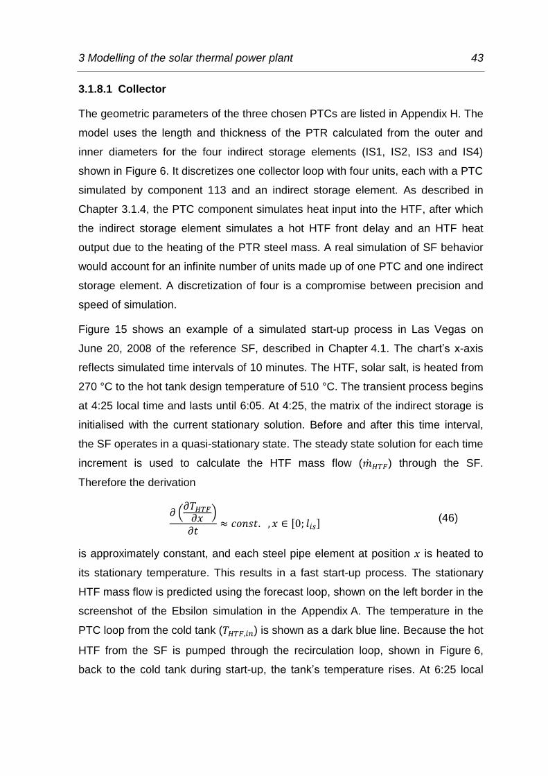
3 Modelling of the solar thermal power plant 43
3.1.8.1 Collector
The geometric parameters of the three chosen PTCs are listed in Appendix H. The
model uses the length and thickness of the PTR calculated from the outer and
inner diameters for the four indirect storage elements (IS1, IS2, IS3 and IS4)
shown in Figure 6. It discretizes one collector loop with four units, each with a PTC
simulated by component 113 and an indirect storage element. As described in
Chapter 3.1.4, the PTC component simulates heat input into the HTF, after which
the indirect storage element simulates a hot HTF front delay and an HTF heat
output due to the heating of the PTR steel mass. A real simulation of SF behavior
would account for an infinite number of units made up of one PTC and one indirect
storage element. A discretization of four is a compromise between precision and
speed of simulation.
Figure 15 shows an example of a simulated start-up process in Las Vegas on
June 20, 2008 of the reference SF, described in Chapter 4.1. The chart’s x-axis
reflects simulated time intervals of 10 minutes. The HTF, solar salt, is heated from
270 °C to the hot tank design temperature of 510 °C. The transient process begins
at 4:25 local time and lasts until 6:05. At 4:25, the matrix of the indirect storage is
initialised with the current stationary solution. Before and after this time interval,
the SF operates in a quasi-stationary state. The steady state solution for each time
increment is used to calculate the HTF mass flow ( ) through the SF.
Therefore the derivation
(
)
[ ]
(46)
is approximately constant, and each steel pipe element at position is heated to
its stationary temperature. This results in a fast start-up process. The stationary
HTF mass flow is predicted using the forecast loop, shown on the left border in the
screenshot of the Ebsilon simulation in the Appendix A. The temperature in the
PTC loop from the cold tank ( ) is shown as a dark blue line. Because the hot
HTF from the SF is pumped through the recirculation loop, shown in Figure 6,
back to the cold tank during start-up, the tank’s temperature rises. At 6:25 local

44 3 Modelling of the solar thermal power plant
time, loading of the hot tank begins, and the temperature of the cold tank becomes
quasi-stationary.
The input temperature of the indirect storage elements is represented by a
dashed, the output temperature by a continuous line. Unit one, consisting of PTC
C1 and indirect storage element IS1, reaches stationary conditions first, followed
after an interval by the other units until the start-up procedure is finished and the
SF begins quasi-stationary operations at 6:05.
3.1.8.2 Header
The model simulates the instationary cascaded header piping with a given number
of branches ( ), shown in Figure 16, using a simple pipe with constant inner
diameter ( ) and length ( ) as representative header model.
This model should have the same thermal inertia as the cascaded header. Thus
the mass of molten salt and the mass of the steel in the representative pipe must
be equal to the corresponding masses of the ideally cascaded header if the same
Figure 15: Simulated start-up process of the solar field with solar salt as HTF from minimum
temperature of 270 °C to operating temperature of 510 °C on June 20, 2008 in Las Vegas
Transient start up procedure Quasi-stationary operation
Quasi-
Stationary
Night
circulation
Load
Hot Tank
Load
Cold Tank
Initialisation of
transient
simulation

3 Modelling of the solar thermal power plant 45
energetic effort during heating is to be obtained. The throughput time of the
representative header should also be equal to the average throughput time of the
original header in order to simulate similar delay (Hirsch 2010).
Therefore the mass of the molten salt in the ideally cascaded header
∑
∑
(47)
can be calculated using the mass flow into the subfield at the design point
( ), the average length of the header pipeline between two PTC rows
from Eq. (25), and the assumed constant design velocity ( ), as outlined in
Chapter 3.1.5. As previously stated, Eq. (47) must be equal to Eq. (48), the
equation to calculate the molten salt mass in the representative pipe ( ).
(48)
Using the maximum inner diameter of the ideally cascaded header as the inner
diameter of the representative pipe, the length of the representative pipe can be
calculated by combining Eqs (47) and (48).
( ) (49)
The steel masses of the representative pipe
Figure 16: Schematic of the distributing header with a specific number of branches adapted
from (Hirsch 2010)
1 2 3
1 2 3 4
321 MMMMMM
mmsubfield
l rowdist2
nm
br
subfield
n br
1 nbrj
n
mmbr
subfieldj
j1

46 3 Modelling of the solar thermal power plant
(( )
) (50)
must also be identical to the steel mass of the ideally cascaded header ( ).
∑
(( )
)
(51)
The model assumes constant thickness ( ) for all elements of the ideally
cascaded header. Combining Eqs (50) and (51) allows the thickness of the
representative pipe ( ) to be calculated. The average throughput time of a
header ( ) with a specific number of branches ( ) can be calculated using the
constant throughput time of a section ( )
∑
∑
(52)
( )
and is equal to the throughput time of the representative header ( ).
3.1.8.3 Feeders 1 and 2
To simulate the thermal inertia of feeders 1 and 2, the model assumes a constant
thickness ( ) and design velocity ( ), as stated in Chapter 3.1.8.2. The inner
diameter of feeders 1 and 2
√
(53)
is calculated using the mass flow through the component at the design point
( ). The length of the feeders is determined using Eq. (24).
Feeder pipe thickness is a further design parameter for thermal optimization. Thick
pipes have a damping effect on the SF. That means that, during start-up, thicker
pipes delay the hot HTF front more because they are able to store more heat. This
effect is reversed during shut-down. It is possible to use thick pipes as passive
heating elements in order to prevent solidification during nighttime operations.

3 Modelling of the solar thermal power plant 47
3.2 Power block
The power block is based on a conventional thermal power plant. The sub-critical
steam generator, a once-through boiler, is the only non-conventional part.
State-of-the-art SGs are based on fossil fuels, e.g. coal or oil, and the heat is
transferred by convection and radiation to the water-steam cycle. In the
once-through boiler with salt as HTF, heat is transferred by convection only, and
the behavior of such an SG is therefore different from state-of-the-art SGs.
The model of the PB is shown in Figure 17. In the SG, the water is heated to
boiling by the economiser (Eco) and then passes the evaporator (Eva) and the
superheater (SH). The resulting live steam with temperatures of up to 540 °C is
fed into the high-pressure stages (HPS1, HPS2) of the steam turbine and reheated
in the reheater (RH) of the SG before it is fed into the five low-pressure
stages (LPS1, LPS2, LPS3, LPS4, LPS5). The mechanical energy produced by
the steam turbine is converted into electrical energy by the generator (G). The
exhaust steam from the steam turbine is converted into water by the
condenser (C). Steam content reaches about 90%. The turbine back-pressure
depends on the type of the cooling system, as well as on ambient factors such as
dry-bulb temperature and humidity (California Energy Commission 2002, p. 4-4).
The condensate is pumped by the condensate pump (CP2) through three feed
water heaters, each consisting of an after cooler (AC1, AC2, AC3) and a
preheater (PH1, PH2, PH3). Extracted steam from the low-pressure turbine stage
is used to preheat the feed water. Low-pressure vapour is also used for preheating
in the feed water tank (D). Finally, the feed water pump (FWP) pumps the fluid
through two further preheaters (AC4, PH4, AC5, PH5), which are fed by extracted
steam from the high-pressure turbine. For off-design operations, the model
assumes live steam extraction (AC6, PH6) to prevent low feed water temperatures
in the economiser resulting in solidification of the salt at the outlet of the SG.

48 3 Modelling of the solar thermal power plant
G
So
lar F
ield
Eco
Eva
SH
RH
S6
HP
S1
HP
S2
LP
S1
LP
S2
LP
S3
LP
S4
LP
S5
C
CP
1
CP
2
FW
P
TH
1
TH
2
TH
3T
H4
TH
5
TH
6
S5M
5
PH
1
PH
2
PH
3P
H4
PH
5
PH
6
AC
1
AC
2
AC
3A
C4
AC
5
AC
6
D
G
Co
mp
4: S
imp
le S
plitte
r
Co
mp
3: M
ixe
r with
thro
ttle
Co
mp
12
4: H
ea
t exch
an
ge
r with
ph
ase
tran
sitio
n
Co
mp
6: S
tea
m tu
rbin
e
Co
mp
11
: Ge
ne
rato
r
Co
mp
7: S
tea
m tu
rbin
e c
on
de
nso
r
Co
mp
83
: Pu
mp
(va
riab
le s
pe
ed)
Co
mp
27
: Afte
rco
ole
r
Co
mp
10
: Fe
ed
wa
ter p
reh
ea
de
r /
He
atin
g c
on
de
nso
r
Co
mp
14
: Co
ntro
l va
lve
Co
mp
9: F
ee
d w
ate
r tan
k /
De
-ae
rato
r
Ph
oto
Ca
ptio
n
Live steam extraction
Steam extraction 1
Steam extraction 2
Steam extraction 3
Steam extraction 4
Steam extraction 5
Steam extraction 6
Fig
ure
17: M
od
el o
f the p
ow
er b
lock w
ith E
bsilo
n
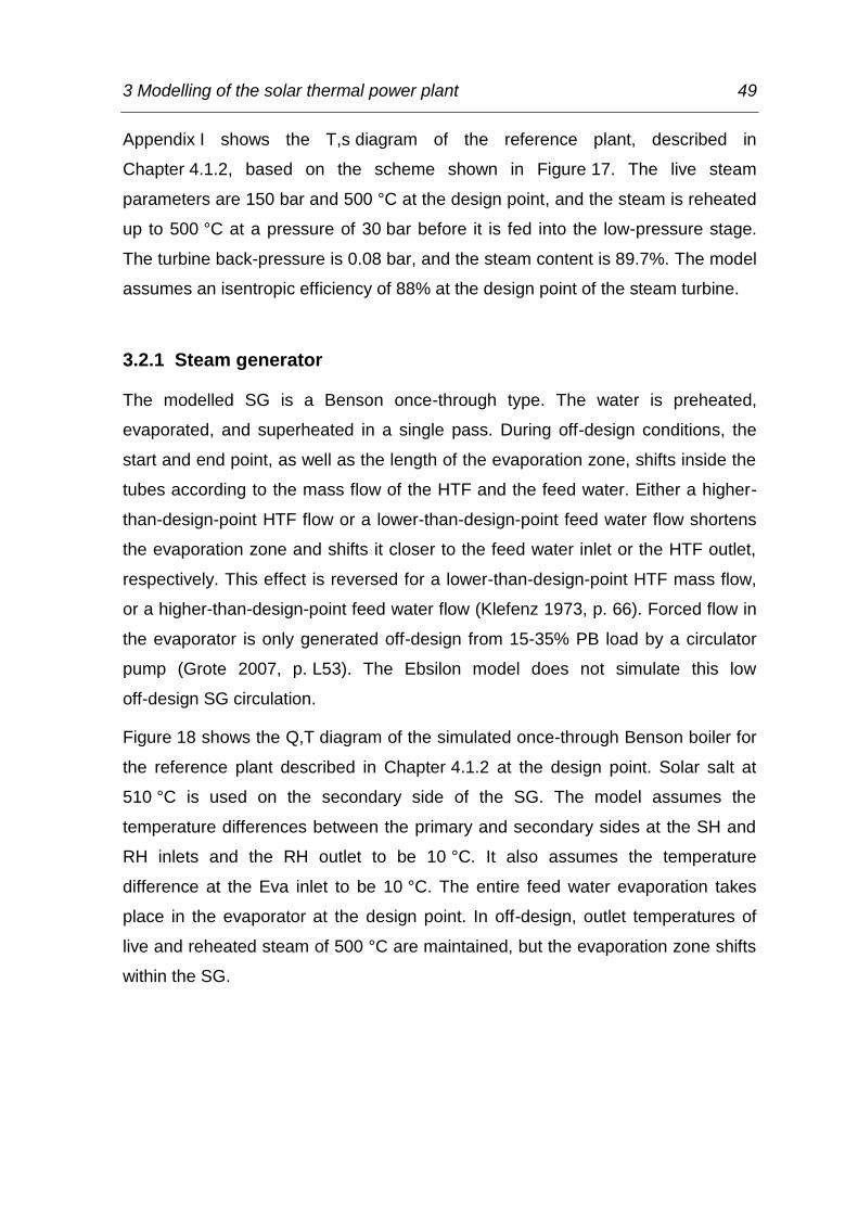
3 Modelling of the solar thermal power plant 49
Appendix I shows the T,s diagram of the reference plant, described in
Chapter 4.1.2, based on the scheme shown in Figure 17. The live steam
parameters are 150 bar and 500 °C at the design point, and the steam is reheated
up to 500 °C at a pressure of 30 bar before it is fed into the low-pressure stage.
The turbine back-pressure is 0.08 bar, and the steam content is 89.7%. The model
assumes an isentropic efficiency of 88% at the design point of the steam turbine.
3.2.1 Steam generator
The modelled SG is a Benson once-through type. The water is preheated,
evaporated, and superheated in a single pass. During off-design conditions, the
start and end point, as well as the length of the evaporation zone, shifts inside the
tubes according to the mass flow of the HTF and the feed water. Either a higher-
than-design-point HTF flow or a lower-than-design-point feed water flow shortens
the evaporation zone and shifts it closer to the feed water inlet or the HTF outlet,
respectively. This effect is reversed for a lower-than-design-point HTF mass flow,
or a higher-than-design-point feed water flow (Klefenz 1973, p. 66). Forced flow in
the evaporator is only generated off-design from 15-35% PB load by a circulator
pump (Grote 2007, p. L53). The Ebsilon model does not simulate this low
off-design SG circulation.
Figure 18 shows the Q,T diagram of the simulated once-through Benson boiler for
the reference plant described in Chapter 4.1.2 at the design point. Solar salt at
510 °C is used on the secondary side of the SG. The model assumes the
temperature differences between the primary and secondary sides at the SH and
RH inlets and the RH outlet to be 10 °C. It also assumes the temperature
difference at the Eva inlet to be 10 °C. The entire feed water evaporation takes
place in the evaporator at the design point. In off-design, outlet temperatures of
live and reheated steam of 500 °C are maintained, but the evaporation zone shifts
within the SG.

50 3 Modelling of the solar thermal power plant
The model assumes the geometry of the SG to be a shell and tube heat
exchanger with countercurrent flow, as shown in Figure 19. To simulate realistic
off-design behavior, the model uses average heat transfer coefficients at the
design point of the primary ( ) and secondary ( ) sides of the SG.
To calculate the heat transfer coefficient of the HTF side, the model assumes a
radial HTF flow around tube bundles and neglects axial flow around the bundles.
Figure 18: Q,T diagram of a steam generator at the design point for a 125-MWe power plant
with solar salt at 510 °C as HTF
Figure 19: Shell and tube heat exchanger adapted from (VDI 2006, p. Cc1)
10 °C temperature difference
saturated steam
saturated water
EVA
Eco
SH
RH
Evaporator Superheater ReheaterEconomiser
molten salt
Molten salt
inlet
Molten salt
outlet
Feed water
inlet
Live steam
outlet
Flow axial to
the tube
bundles
Flow radial
to the tube
bundles

3 Modelling of the solar thermal power plant 51
Assuming the outer tube diameter ( =0.034 m), and the velocity of the molten
salt through the SG at the design point ( =0.35 m/s), the average heat
transfer coefficient at the design point of the Eco, Eva, SH, and RH ( ) can
be calculated (Polifke 2005, p. 229f)
(54)
by using the average HTF properties over the Eco, Eva, SH, and RH to calculate
the Nusselt, Reynolds, and Prandtl numbers. The average heat transfer
coefficients of the primary side at the design point of the Eco, SH, and RH
( ) can be calculated, assuming the inner tube diameter ( =0.030 m)
and the velocity of the water through the SG at the design point ( =1 m/s)
(Polifke 2005, p. 233).
(55)
The average speed of the steam at the design point in the SH and RH
(56)
can be calculated from the mass conservation, assuming constant areas in Eco
and SH. To calculate the average heat transfer coefficients of the Eva at the
design point ( ), (VDI 2006, p. Cc1) proposes an overall heat transfer
( - ) of between 900 and 3000 W/m²/K. Letting - 2200
W/m²/K, using the average heat transfer coefficient of the HTF in the Eva
( ) from Eq. (54), and assuming the heat conductivity ( ) of 25
W/m/K,
(57)
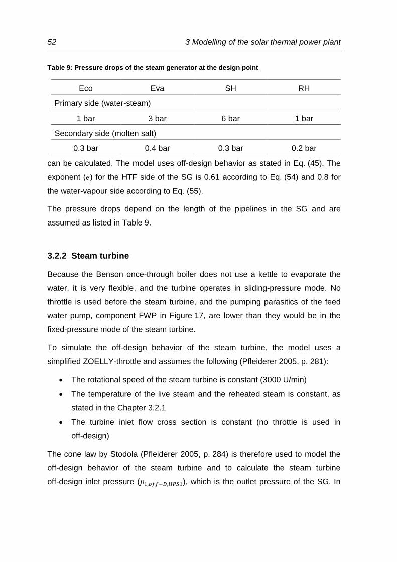
52 3 Modelling of the solar thermal power plant
can be calculated. The model uses off-design behavior as stated in Eq. (45). The
exponent ( ) for the HTF side of the SG is 0.61 according to Eq. (54) and 0.8 for
the water-vapour side according to Eq. (55).
The pressure drops depend on the length of the pipelines in the SG and are
assumed as listed in Table 9.
3.2.2 Steam turbine
Because the Benson once-through boiler does not use a kettle to evaporate the
water, it is very flexible, and the turbine operates in sliding-pressure mode. No
throttle is used before the steam turbine, and the pumping parasitics of the feed
water pump, component FWP in Figure 17, are lower than they would be in the
fixed-pressure mode of the steam turbine.
To simulate the off-design behavior of the steam turbine, the model uses a
simplified ZOELLY-throttle and assumes the following (Pfleiderer 2005, p. 281):
The rotational speed of the steam turbine is constant (3000 U/min)
The temperature of the live steam and the reheated steam is constant, as
stated in the Chapter 3.2.1
The turbine inlet flow cross section is constant (no throttle is used in
off-design)
The cone law by Stodola (Pfleiderer 2005, p. 284) is therefore used to model the
off-design behavior of the steam turbine and to calculate the steam turbine
off-design inlet pressure ( ), which is the outlet pressure of the SG. In
Table 9: Pressure drops of the steam generator at the design point
Eco Eva SH RH
Primary side (water-steam)
1 bar 3 bar 6 bar 1 bar
Secondary side (molten salt)
0.3 bar 0.4 bar 0.3 bar 0.2 bar

3 Modelling of the solar thermal power plant 53
Eq. (58), the pressure at the inlet of the steam turbine stage is marked with the
subscript and at the outlet with .
√(
)
(
)
(58)
The model assumes no pressure losses or leakages between turbine stages. This
Eqs (58) can therefore be solved, since the outlet pressure of the LPS5 (the
turbine back-pressure) is assumed to be constant. The parameters at the design
point of the turbine stages are listed in Table 10.
Mechanical efficiency is assumed to be constant, whereas the isentropic efficiency
is lower in off-design. This characteristic of the steam turbine depends on the ratio
of volume flow in off-design to volume flow at design point and is adopted from the
Ebsilon pre-set.
3.2.3 Condenser and cooling system
As stated in Chapter 3.2.2, the model assumes the turbine back-pressure to be
constant. It therefore ignores correlation with the dry-bulb ambient temperature or
the humidity because the Ebsilon model does not simulate the cooling system.
Wet cooling systems have the best performance, are relatively independent of
ambient temperatures, and allow turbine back-pressures as low as 0.07 bar. Dry
cooling systems have lower performance with turbine back-pressure as high as
Table 10: The parameters of the steam turbine at the design point
HPS1 HPS2 LPS1 LPS2 LPS3 LPS4 LPS5
Pressure [bar]
Inlet 150 51 30 16 10 4.50 1.50
Outlet 51 31 16 10 4.50 1.50 0.07-0.5
Efficiency [-]
Isentropic 0.880
Mechanical 0.998

54 3 Modelling of the solar thermal power plant
0.5 bar. Hybrid cooling systems combine both technologies, and the resulting
turbine back-pressure is between those of the dry and wet cooling systems (NREL
2009, p. 14ff). Ebsilon models the cooling system indirectly by assuming a
constant turbine back-pressure. The secondary fluid of the condenser, the cooling
fluid, has a constant temperature of 20 °C at the inlet and 30 °C at the outlet.
3.2.4 Feed water heating
Figure 20 shows the feed water heating in the PB, during which condensers (PH1
to PH5) condensate the extracted steam from the turbine stages. Aftercoolers
(AC1 to AC5), past the condensers, further increase the feed water’s temperature.
The components AC6 and PH6 are only activated in low PB off-design. The model
assumes the temperature difference at the outlets of these components to be 5 °C
and the pressure drop of the primary fluid, the feed water, to be 0.05 bar in each
component.
Figure 20: Q,T diagram of the feed water heating at the design point for a 125-MWe power
plant with solar salt at 510 °C as HTF – AC6, PH6 are not active
PH1
AC2AC1 AC3
AC4
AC5
PH2
PH3
PH4
PH5
Feed water
from condenser
Feed water
to steam generatorExtracted steam
from LPS4
Extracted steam
from LPS3
Extracted steam
from LPS2 Extracted steam
from HPS2
Extracted steam
from HPS1
Heating in feed
water tank with
extracted steam
from LPS1

3 Modelling of the solar thermal power plant 55
3.2.5 Live steam extraction and off-design of the power block
Chapters 3.2.1 and 3.2.2 describe the off-design behavior of the SG and the
steam turbine, respectively. The model also uses off-design behavior, as
described in (45), for all heat exchangers. Figure 21 shows the off-design behavior
of the entire 125-MW power plant with solar salt at 510 °C as HTF, as described in
Chapter 4.1.2. The pressure of the live steam, the yellow line in Figure 21, falls
linearly with the PB load. Because the turbine back-pressure is nearly zero,
(59)
this linear characteristic can be calculated using Eq. (58). The salt mass flow into
the SG is also nearly directly proportional to the PB load until the live steam
extraction is activated because the temperature of the molten salt at the outlet of
the Eco should not fall below its threshold temperature. As Figure 21 shows, at
57% PB load, the temperature of the HTF is close to the threshold temperature,
and live steam is extracted. This is the reason for the lower gradient of the salt
mass flow into the SG between 35% and 57% load. The PB efficiency also
decreases faster when live steam is extracted. During off-design, the relative mass
flow through the Eco, Eva, and SH
Figure 21: Off-design behavior for a 125-MWe power plant with solar salt at 510 °C as HTF
Live steam extraction
is necessary
56 3 Modelling of the solar thermal power plant
(60)
increases because the vapour pressure decreases, and the relative heat input
required to evaporate the feed water
(61)
is therefore higher. This is why the gradient of the salt mass flow into the Eco, Eva,
and SH, over the PB load, is lower than that of the SG salt mass flow. Both are
shown in Figure 21.
3.2.6 Pseudo-transient behavior of the power block
The transient behavior of the PB is not modelled as much detail, as that of the SF,
described in Chapter 3.1.8. Instead of modelling full transient behavior, the model
assumes a pseudo-transient one. An energy state of the PB ( ) is therefore
introduced that models the current energy stored in the power block.
( ) ∫
∑
(62)
Eq. (62) takes the thermal energy flow into the PB ( ) at a specific time
instant ( ) with the time series time step ( ) in account.
All component masses in the PB ( ), e.g. the water, the steel masses of the
pipes, the heat exchangers, and the turbine, are heated from the start temperature
( ) to average design temperature ( ) during start-up procedure.
Therefore the energy
∑ ( )
(63)
is stored in the PB. Because this required start-up PB energy is difficult to
simulate, the model uses a more simplified ansatz.

3 Modelling of the solar thermal power plant 57
(64)
A start-up time ( ) is introduced to estimate the thermal power needed for
PB start-up. This time is multiplied by the thermal input of the power block at the
design point ( ) and is assumed to be from 0.5 to 1 hour. This start-up
time increases as with PB downtime. Because the literature provides no cool-down
data for a PB with a once-through boiler and salt as HTF, the model assumes that
PB heat losses during standby operations ( ) are 1% of PB thermal
energy input during operations at the design point ( ).
(65)
During PB standby mode, a salt mass flow corresponding to passes
through the SG, and as a result, the start-up time ( ) is assumed to be
constant. The PB start-up state
( )
(66)
can be calculated by combining Eqs (64), and (62), and is between 0, or unheated,
and 1, or ready for energy production.
Besides the PB thermal inertia, the start-up process is also delayed due the mass
inertia of the steam turbine. High temperature gradients are also to be avoided to
reduce thermal strain, so the speed of the heating process is limited. To account
for these factors, the simulation introduces the ramp-up factor ( ) with the unit
[kg/s/s]. This factor allows the mass flow into the PB at a given time
( ) ( ) ∑ ( )
( )
(67)
to be calculated using the mass flow into the SG at 30% PB load ( )
and the beginning time of the start-up ( ).
Figure 22 shows an example of the modelled pseudo-transient PB behavior
located in Las Vegas on the January 1, 2008, simulated in ten-minute resolution.

58 3 Modelling of the solar thermal power plant
After reaching a specific hot tank level at 12:35, the PB starts to operate at 30%
load. The mass flow into the SG increases linearly by the ramp-up factor until it
reaches 100% of PB load, or 125 MWe. Then the PB operates in quasi-stationary
mode at 100% load. The load is slightly reduced until shut-down at 17:15 due to
hot tank cool-down. The dashed red line corresponds to the simulated output of
electric energy. The continuous dark red line corresponds to the real electric
output calculated from the state of the power block given by Eq. (66). Between
13:25 to 13:35, the PB start-up state ( ) reaches 1. Note that the excess thermal
energy at this time instant is counted against electrical output, so reduced
electrical output is plotted starting at 13:25.
3.3 Plant operation management
The simulation model consists of three separate units:
The solar field, shown in Figure 6 and examined in Chapter 3.1
The auxiliary heater, shown in Figure 13 and examined in Chapter 3.1.7
The power block, shown in Figure 17 and examined in Chapter 3.2
Figure 22: Simulated start-up procedure of the power block from 30% load (37.5 MWe) to
100% load (125 MWe) in ten-minute resolution in Las Vegas on January 1, 2008
Start-up at
30% PB load
Ramp-up = 100kg / 10min
Shut down of the
power block
Power block is ready to
prodcue electricity
t_start-up = 30 min
100% PB loadstandby
Start-
up

3 Modelling of the solar thermal power plant 59
Because of the SF’s ability to operate in stationary or transient mode, twelve
different possible solar thermal power plant operation modes are possible, all
shown in Table 11. The Ebsilon model uses eight of them, listed in Table 11 as
profiles (P) 1 to 8. It neglects the other four possibilities because they require a
more detailed plant operation strategy, e.g supporting the SF during start-up with
hot HTF from the AH (profile XX0), producing hot HTF with the AH during
nighttime and operating the PB in low off-design mode (0XX), or a combination of
both (XXX).
Before the model simulates a given time instant, the EbsScript schematically
shown in Appendix G selects a profile. Each profile imports various process
Table 11: Solar thermal power plant operation mode possibilities and the implemented
profiles (P)
Steady state of the PTCs
P SF AH PB Description
1 X 0 X stationary SF and PB operation, AH is off
2 X 0 0 Stationary SF operation, PB is on standby, AH is off
3 0 0 X SF is on standby, stationary PB operation, AH is off
4 0 0 0 SF and PB are on standby, AH is off
5 0 X 0 SF and PB are on standby, AH supports HT
n/a X X 0 Stationary SF operation, PB is on standby, AH supports SF, HT, or
both
n/a 0 X X SF is in standby, PB operates stationary, AH supports HT
n/a X X X Stationary SF and PB operation, AH supports SF, HT, or both
Transient state of the the PTCs
P SF AH PB Description
6 X 0 X Instationary SF operation, stationary PB operation, AH is off
7 X 0 0 Instationary SF operation, PB is on standby, AH is off
8 X X 0 Instationary SF operation, PB is on standby, AH supports SF, HT,
or both
n/a X X X Instationary SF operation, stationary PB operation, AH supports
SF, HT, or both

60 3 Modelling of the solar thermal power plant
parameters into the simulation model. The profile selection process is shown in
Appendix J. The first step is determining whether the PTC simulation mode is
steady or transient. Then the threshold hot tank level for AH operation is identified
according to time of day. During daytime, the SF can operate if a minimum
predicted salt mass flow from the SF is secured. This salt mass flow is forecasted
with the “Forecast of salt mass flow“ module, shown on the left side of the
screenshot in Appendix A. The PB is able to operate if the hot tank minimum level
is reached. This threshold level changes dynamically each day according to
weather conditions. Then the PB operates until an HT threshold level is reached.
Figure 23 shows the schematic of the Ebsilon simulation mode selection. To
improve simulation speed, the model uses two separate instationary units:
The four PTCs (IS1, IS2, IS3, IS4 in Figure 6), named C unit
The header and feeder pipelines (IS5, IS6, IS7 in Figure 6), named H-F unit
These two instationary units can change the simulation mode from steady to
transient or vice versa. If the C unit simulation mode is transient, the H-F unit
simulation mode is also transient. The thermal state of the header and feeders is
therefore only assumed to be steady if the SF operation is also steady. A transient
simulation starts at sunrise. This process is marked red in Figure 23. The C unit is
transient until the HTF temperature after the H2 component, shown in Figure 6, is
above hot tank design temperature, or until the HTF temperature is below the
lowest HTF temperature during nighttime circulation and the sun has set. This
occurs when there is not enough solar radiation to start-up the SF during daytime.
Transient processes during daytime, e.g. clouding or end-of-day shut-down, are
marked blue in Figure 23. If the SF changes its status from operational to
non-operational or vice versa in succeeding time instants, the model initialises a
transient simulation which lasts until the hot tank design temperature or the lowest
HTF nighttime circulation temperature is reached. The H-F unit is always assumed
to be steady when these temperatures are reached after the IS7 component,
shown in Figure 6. As shown in Table 11, a profile is considered transient if the
instationary unit of the PTC is transient. This is because the numeric controller
regulating the SF outlet temperature can only operate during C unit stationary
operation.

3 Modelling of the solar thermal power plant 61
Fig
ure
23:
Sch
em
ati
c o
f th
e s
imu
lati
on
mo
de s
ele
cti
on
im
ple
men
ted
in
Eb
sil
on
SF s
tan
db
yC
un
it: s
tead
yF-
H u
nit
: tra
nsi
ent
SF s
tan
db
yC
un
it: s
tead
yF-
H u
nit
: ste
ady
SF o
per
atin
gC
un
it: t
ran
sien
tF-
H u
nit
: tra
nsi
ent
SF o
per
atin
gC
-un
it: s
tead
yF-
H u
nit
: tra
nsi
ent
SF o
per
atin
gC
-un
it: s
tead
yF-
H u
nit
: ste
ady
sun
set
AN
D T
_SF_
1<T
_HTF
_lo
w
T_SF
_2<T
_HTF
_lo
wsu
nri
seT_
SF_1
>T_H
T_D
T_SF
_2>T
_HT_
D
T_SF
_2<T
_HTF
_lo
wD
uri
ng
day
OP
_SF_
nex
t=1
T_SF
_1>T
_HT_
DT_
SF_2
>T_H
T_D
T_SF
_1<T
_HTF
_lo
w
sun
rise
Du
rin
g d
ayO
P_S
F_n
ext=
1
Du
rin
g d
ayO
P_S
F_n
ext=
0
Du
rin
g d
ayO
P_S
F_n
ext=
0
T_SF
_1T_
SF_2
T_H
T_D
T_H
TF_l
ow
OP
_SF_
nex
t
Tem
per
atu
re a
fter
H2
in f
igu
re 6
Tem
per
atu
re a
fter
IS7
in f
igu
re 6
Des
ign
tem
per
atu
re o
f th
e h
ot
tan
kLo
wes
t te
mp
erat
ure
of
the
HTF
fo
r n
igh
t re
circ
ula
tio
nO
per
atio
n m
od
e o
f th
e so
lar
fiel
d in
th
e n
ext
tim
e in
stan
t0
à S
ola
r fi
eld
can
no
t o
per
ate
du
e lo
w r
adia
tio
n1
à S
ola
r fi
eld
can
op
erat
e
Ph
oto
Cap
tio
n
Tran
sien
t st
art-
up
pro
ced
ure
du
rin
g d
ay m
arke
d b
lue
(can
beg
in a
t b
lack
cir
cles
)
Tran
sien
t st
art-
up
pro
ced
ure
at
sun
rise
mar
ked
red
(ca
n b
egin
at
bla
ck c
ircl
es)
Tran
sien
t sh
ut-
do
wn
pro
ced
ure
du
rin
g d
ay m
arke
d b
lue
(can
beg
in a
t b
lack
cir
cles
)

62 3 Modelling of the solar thermal power plant
The control of the instationary units is simulated using the Ebsscript shown in
Appendix G.
As previously stated, the minimum hot tank level for a given day’s PB operations
depends on weather conditions. The decision criteria are the day’s maximum DNI
( ( ) ( )) (68)
and the day’s average DNI.
∫ ( ) ( )
(69)
There are four types of day:
Very bad day: (PB does not start)
Bad day: (PB starts at load)
Good day:
(PB starts at load)
Very good day:
(PB starts at load)
For each day, a threshold hot tank level for PB operations is specified. When this
level is reached, the PB operates until the hot tank level falls below a threshold
level. These plant operation management parameters are listed in the table in
Appendix C under “Parameters to identify the weather conditions of a day” and
“Parameters to identify whether power block can operate”.
Another profile changes is hot tank load during transient processes. During start-
up or shut-down, the HTF is recirculated over the recirculation loop shown in
Figure 6. If the HTF has reached a specific upper temperature before component
S3, shown in Figure 6, it is pumped into the hot tank, as shown in Figure 15.
During start-up, the cold tank temperature (the dark blue line in Figure 15) rises
until the hot HTF is pumped into the hot tank.

3 Modelling of the solar thermal power plant 63
To prevent the HTF from solidifying in the SF, it is pumped via the recirculation
loop shown in Figure 6 during night operation, taking advantage of the thermal
energy stored in the cold tank during shut-down. If the cold tank temperature falls
below design temperature, HTF from the hot tank is pumped through the cold tank
support loop shown in Figure 6. If the hot tank falls below a critical load level, the
AH is activated to support it. HTF from the cold tank is pumped to the AH, heated,
and pumped via the hot tank support loop, shown in Figure 6, to the hot tank in
order to raise its level.
3.4 Calculation procedure of the levelized electric costs
To compare the simulated solar thermal power plant with other configurations, the
levelized electric costs (LECs) are calculated according to the “Guidelines for the
economic analysis of renewable energy technology applications” (International
Energy Agency 1991, p. 90ff). Figure 24 shows the calculation procedure. First the
Ebsscript “Design power plant”, shown in Appendix F, calculates the characteristic
parameters of the PB, such as the total SF gross aperture area ( ), the total
PP area ( ) and the tank thermal capacity ( ), according to the user input
parameters. The power plant annual yield calculation for a characteristic year
reveal the annual net electric output of the power plant ( ) and the annual
thermal energy input of the gas ( ). These parameters and the design gross
electrical output ( , a user input parameter) allow calculation of the LECs in
€/kWhe using the economic and statistical model presented in this chapter.
3.4.1 Economic model
The LEC is the ratio of all costs the power plant generates during one year to its
annual net electric output. These costs are the annual cost for gas ( ), insurance
( ), and operation and maintenance ( ). The total investment cost ( ) at the
beginning of the project, the year zero, is multiplied by the capital recovery factor
( ) in order to convert it into an annual value over the project lifetime. The

64 3 Modelling of the solar thermal power plant
(70)
is calculated by combining Eqs (70), (71), (72), (73), (74), (75), and (76). The cost
for gas
(71)
is calculated using the annual thermal energy input of the gas, the efficiency of the
AH, and the cost of the gas ( ) in €/MWhth. The cost of insurance
(72)
is calculated using the total investment cost and the factor . The
operation and maintenance costs
(( ) ) (73)
cover costs for staff, water consumption and treatment, and equipment. A fixed
number of employees ( ) for the BOP and a number of employees for SF
maintenance
Figure 24: Schematic of the economic model to calculate the levelized electric costs
Economic
and Statistic
Model
Parameters from the
design of the power
plant with the Ebsscript
shown in Appendix F
Parameters from the
annual yield calculation
with the time series
cumulative density function and
probability density function of the
LEC
Aperture
area of the
solar field
Total area
of the plant
Design
gross
electrical
output
Thermal
capacity of
the storage
Annual net
electric
output
Gas
consumption
User input

3 Modelling of the solar thermal power plant 65
(74)
that depends on the total gross aperture area of the SF, and the factor
in 1/1000m², is multiplied by the cost per employee ( ) in €/a. The
cost of water consumption and treatment depends on the specific water
consumption costs ( ) in €/MWhel and on the net electric output of the power
plant. The cost for equipment depends on the total investment cost and the factor
. The annual OM factor ( ) allows adjustment of operation and
maintenance costs because of regional differences, for example.
The total investment cost is the sum of costs for the power block ( ) in €/kWe,
SF ( ) in €/m², storage system ( ) in €/kWhth, land in €/m², and indirect
costs of construction, calculated using the factor .
( )( ) (75)
To convert the total investment cost into an annual value over the project lifetime,
the capital recovery factor
( )
( ) (76)
is calculated using the project lifetime ( ) and the real discount rate of the project
( ).
3.4.2 Statistical model
As stated in Chapter 2.6, no commercial PTC power plant with molten salt as HTF
is in operation, and only research and development projects have been carried out
so far. For this reason, no exact data about the specific cost, e.g. the cost of the
SF or storage system, is available. Many external parameters such as regional,
political, or financial considerations, also influence the LECs. The LECs are
therefore to be understood as estimates.
To account for all these uncertainties, the Matlab script shown in Appendix K
calculates the LECs using a Monte Carlo simulation based on a random sampling
of input parameters into a function ( ). In the specific case

66 3 Modelling of the solar thermal power plant
of the economic analysis, the parameter corresponds to the LECs and the
parameters to the input parameters in the economic model. Before each
simulation, the input parameters are selected individually according to their
predefined probability distribution. Then the function is calculated. Repeating
this process for several iterations provides a distribution function of the value ,
which is equal to the probability of a range of values. The accuracy of this
simulation depends on the number of simulation iterations and the number of input
parameters. Therefore only parameters with appreciable effect on are taken in
account. The cost for land, for example, is assumed to be constant because its
effect is negligible.
To specify the probability distribution of the input parameters, the continuous
uniform distribution and normal distribution are selected. The continuous uniform
distribution is a distribution of values between a minimum and maximum value.
Each number in this interval is equally probable. This function is selected when no
data about probability of a value is available and only the minimum and maximum
values can be estimated. This is the case for the cost of SF or the real discount
rate of the project, for example. Because no commercial SFs with molten salt as
HTF have so far been built, only data about SFs with Thermoliquid as HTF and
their minimum and maximum costs are available. The real discount rate depends
on the inflation rate, debt interest rate, equity rate, ratio of debt to equity financing,
and political grants, so no exact probabilities for this value can be estimated. The
normal distribution function
( )
√
( )
(77)
is used if the a parameter value is relatively fixed and therefore its variation is not
as high. The mean value ( ) and the standard deviation of 99% for all values
(2.576 ) are used to calculate the distribution function in Eq. (77). The PB, for
example, is an established conventional technology, and its cost is relatively
well-known. The normal distribution is therefore selected.

3 Modelling of the solar thermal power plant 67
The probability density function (pdf, ( )) and the cumulative density function
(cdf, ( )) are used to visualise the probability of a given parameter. Between the
pdf and cdf, the following correlation can be stated (Merziger 2007, p. 197).
( ) ∫ ( )
(78)
According to the central limit theorem (Merziger 2007, p.202), the mean values of
independent and identically distributed input parameters ,
∑
(79)
is normally distributed, as Eq. (77) shows, and asymptotic for an infinite number of
iterations ( ). Each mean value of the parameters is therefore asymptotic,
and, as a result, the mean value of the function ( ) is also asymptotic.
To identify a suitable number of iterations, the residuals of the mean LEC ( ) is
taken in account. The more Monte Carlo experiments undertaken, the closer
will approximate its exact value. The residual decreases linearly with the number
of experiments. A number of 1,000,000 and therefore residuals of is assumed
to be exact enough.
Because both continuous uniform distributions and normal distributions are used
to calculate the LECs, the resulting pdf is not identical to the normal distribution
function in Eq. (77), and therefore the mean, mode, and median LEC value are not
necessarily equal.

68 4 Application of the solar thermal power station model
4 Application of the solar thermal power station model
This chapter investigates the performance of the solar thermal power station
model by applying it to a reference plant. It compares quasi-stationary and
transient simulations, as well as simulations with four different time steps in the
time series calculation, with respect to the reference plant. It also compares the
economic performance of the reference plant at three locations with different direct
normal irradiation averaged annual sums by calculating the power plant‘s LECs
and presents an improved power plant. Finally, it outlines the economic impact of
the cooling method.
4.1 The reference plant
To investigate the performance of the solar thermal power station model, the
results of a reference plant are presented in Chapter 4.2. This chapter outlines the
reference plant’s SF and PB in detail. Las Vegas has been chosen as the
reference plant location. The DNI and temperature inputs into the simulation are
made from the 2008 Las Vegas solar data set. More details about the location and
solar data selection process are found in Appendix M. The parameters used for
the reference plant are listed in Appendix L.
4.1.1 Solar field
The solar field’s layout is the 2 H layout, which consists of 352 collector loops,
each consisting of four Eurotrough ET150 collectors, whose parameters are listed
in Appendix H. In all, the gross aperture area is 1.21 km². The solar multiple of the
solar thermal power plant, the ratio of thermal power from the SF at the design
point ( ) to thermal power into the PB at 100% load ( )
(80)

4 Application of the solar thermal power station model 69
is assumed to be 2.233. Each storage tank has a capacity of 33,555 metric tons of
solar salt and is able to feed the steam generator for 10 hours to produce
electricity. The design temperature is assumed to be 510 °C for the hot tank and
310 °C for the cold tank. During transient start-up or shut-down, the molten salt
from the SF is pumped to the hot tank if its temperature is higher than 485 °C, and
to the cold tank if its temperature is lower. The lowest temperature of the solar salt
during night operations is assumed to be 270 °C in order to ensure a safety
clearance above the molten salt’s liquidus temperature (240 °C).
The velocity of the HTF in the header and feeder pipes is assumed to be 2.5 m/s,
and its heat losses to be 200 W/m. This is equal to 4.0 watts per square meter of
aperture area (4.0 W/m_Ape^2). The thickness of the pipes is assumed to be 71
mm, which results in a steel weight of 1,789 t. The HTF mass in the pipes is
3,115 t. The hot tank’s heat losses are calculated using Eq. (33) at 1.1 K/d at full
tank level.
The solar thermal power plant’s design date is assumed to June 21, 2008 with a
DNI of 850 W/m² and an ambient temperature of 30 °C. Its efficiency on the design
date is 67.20%.
4.1.2 Power block
The PB’s gross capacity is 125 MW, and the live steam parameters are 500 °C
and 150 bar. The turbine back-pressure is assumed to be 0.08 bar, which
corresponds to wet cooling. The SG’s Q,T diagram is shown in Figure 18, and
Figure 20 shows the diagram of the feed water heating. Table 10 lists the
parameters of the modelled steam turbine. The PB’s gross efficiency at the design
point is 44.25%, and its net efficiency 43.86%. The PB’s off-design behavior is
shown in Figure 21. The parameters for the pseudo-transient behavior of the PB,
as described in Chapter 3.2.6, are assumed to be 100 kg/s/(600s) for the ramp-up
factor, and 0.5 h for the start-up time. An example of the PB’s start-up procedure is
given in Figure 22.

70 4 Application of the solar thermal power station model
4.2 Simulation of the reference plant
The solar thermal power station in Las Vegas during 2008 was simulated using the
time series dialog within a ten-minute resolution. A ten-second resolution has been
chosen for component 119 in order to simulate the transient processes during
start-up, shut-down, and periods of low radiation. In all, this results in 52,704
simulations in the time series dialog, lasting for 11.7 hours of wall clock time at
common work station. During the simulation, 16 errors occurred, and
1,743 simulations did not converge to the desired residuals of . The numerical
accuracy, plant operation management, and the results of the simulation are
presented in this chapter.
4.2.1 Numerical accuracy
As stated in Eq.(43), the discretization of component 119 in the x-direction has
been chosen, so that the maximum Courant number is less than one. The maximal
Courant numbers can be observed when the mass flow into the SF is maximal.
They are 0.32 for the PTCs, 0.75 for the header, 0.51 for feeder 2, and 0.88 for
feeder 1. For the summer period of the simulated year, involving high mass flows
into the SF and high temperature gradients due to high radiation, numerical errors
occur during the simulation. A simulation check is therefore implemented into the
simulation model, as shown in Appendix G. The check first changes the mass flow
into the SF, changing the Courant number, and re-simulates the time instant. If the
numerical error still appears, the simulation mode of the instationary component
that causes the error is set from transient to stationary. This simulation check was
carried out 224 times during the simulated year, which represents 0.4% of the total
instants of time. Each simulation check causes a dumping of thermal energy
stored in the HTF and steel mass of the instationary component, which results in
an additional thermal loss, as stated in Figure 26 (heat loss switch
steady-->transient). That loss is 8 GWh, or 0.26% of solar heat input.
Thermal loss can also be observed during SF shut-down. The HTF’s temperature
in the SF ( ( )) falls from the temperature at the first instationary iteration step

4 Application of the solar thermal power station model 71
( ( ) 510 °C) to its lowest temperature during nighttime operations
( 270 °C) within an exponential function
( ) ( ) ( ( ) ) (81)
where the factor is about 60 minutes. This causes very long shut-down
procedures, long transient calculations, and therefore long simulation wall clock
time. To avoid this, the instationary process is stopped if the HTF reaches the
temperature , causing an additional dumping of energy.
∑
(82)
To obtain more precise results, the whole year can be calculated in transient mode
by setting the factor in the implemented user interface to one,
which results in very long simulation wall clock times (up to ten times longer). The
error in Eq. (82) is 8.2 GWh. As shown in Figure 26, the total error of the indirect
storage components ( ), from Eq. (82) and the simulation check, is 16.2
GWh, or 0.5% of the total solar energy input. It can be credited as additional SF
heat loss, or in a first approximation as additional PB electric output.
(83)
As previously stated, the most unstable part of the simulation is the transient
system behavior of the SF during high temperature gradients, e.g. during SF
start-up. The simulation also did not converge to the desired residuals of for
3.3% of all performed simulations, mostly during instationary operations. To
investigate the numerical error over the entire simulated year, the SF energy
conservation is modelled as shown in Figure 26. The SF’s energy output is
calculated using Eqs (84) and (85). Eq. (84) uses the heat flow of the sun ( ),
PTC optical loss ( ), PTR thermal loss ( ), piping thermal loss
( ), and indirect storage thermal loss ( ) for each time step ( ) with a
time interval of ten minutes ( ) to calculate the SF’s total energy output

72 4 Application of the solar thermal power station model
( , ). Eq. (85) uses the energy flow into the SF system ( ) and out of
the system ( ), where S3 and M1 refer to the components in Figure 6.
∑
(84)
∑
∑
(85)
As shown in Figure 26, the numerical error is 0.7 GWh, calculated by subtracting
Eq. (84) from Eq. (85). This corresponds with over the entire year and is
smaller than the maximum possible residuals, assuming residuals of for all
52,704 simulated instants of time.
(86)
The first two result value figures can therefore be said to be numerically exact,
considering the worst case in Eq. (86), up to four, considering the tested case in
Eq. (84) and (85).
4.2.2 Plant operation management
The plant operation management strategy, described in Chapter 3.3, is based on
each day’s weather classification, as shown in Figure 25 a). Seven very bad days
with a maximum DNI of less than 300 W/m² occurred. During these days, the PB
did not start at all. In all, the PB did not operate on 31 days, which means that on
24 bad days, with an average DNI as high as 500 W/m², the 30% threshold level of
the hot tank was not reached. The solar heat input was stored in the hot tank and
used to maintain the SF’s temperature or to feed the SG on the next day. On
335 days, the PB was able to operate. The PB operation threshold level was set to
10% for good days (average DNI from 500 to 800 W/m²) and 4% for
very good days (average DNI higher than 800 W/m²). In all, the PB carried out
338 start-up processes, as described in Chapter 3.2.6. This means that on three
days, the PB had to start-up a second time because the hot tank threshold level

4 Application of the solar thermal power station model 73
(4% load) was reached within the day. On these days, the PB was heated twice,
resulting in higher energy input for heating and more time in off-design mode.
The PTCs were defocused for 14.96% of the SF operation time. That means that
thermal energy of the sun was dumped by setting the focus factor in Eq. (11) to a
value in between 0 to 1. This happened on 145 days between March 18 and
September 24, most of which are during summer. The PTCs remained defocused
on 28 good days.
The ideal operation management strategy would prevent more than one PB
start-up process per day, setting the hot tank threshold level to the correct load
level. But late PB start-ups during days of high solar radiation, resulting in solar
power dumping by defocusing the PTCs, must also be prevented. As outlined, this
happened on 28 good days (threshold level of 10% load) during the 2008 Las
Vegas simulation. The operation management strategy therefore has the potential
to improve with the optimization of the parameters , ,
and . But a perfect operation management strategy is not realistic
because during real-life power plant operations, a late or early PB start-up,
resulting from an inaccurate weather forecast, for example, is also possible.
Figure 25 b) shows the percentages of the selected profiles, as listed in Table 11,
during the simulated year. A transient profile, which refers to transient C unit
components, was necessary 23% of the total time because of the SF start-up
process (mode 1, 42% of transient simulation), and shut-down or clouding
Figure 25: Classification of 2008 in Las Vegas in a) weather conditions and b) selected
profiles

74 4 Application of the solar thermal power station model
(mode 2, 58%). The F-H unit was in transient mode for 31% of the total time. Only
during time instants with high temperature gradients in the SF was a transient
simulation selected, which resulted in 69% of quasi-stationary simulations over the
entire simulated year. During 3.3% of the year, only the SF was operating in quasi-
stationary mode, a condition which is attributable morning operations, when the
hot tank threshold level for PB operations had not yet been reached. In the most
commonly used profile, 29.2% of the time, the PB and SF operated in a quasi-
stationary manner at the same time. 17.7% of the time, only the PB operated, a
condition which is attributable to nighttime periods. In all, the PB is in operational
mode during 57.9% of the simulated time. The SF operates 32.4% of the time in
quasi-stationary SF mode, a figure which rises to 55.4% if transient modes, e.g.
during shut-down, are also included. The nighttime profile, which refers to quasi-
stationary operations during nighttime, was used 27% of the simulated time.
During these times, the PB is in standby mode, and HTF from the cold tank is
pumped through the SF, reaching the lowest HTF temperature (270 °C) at its end.
If the cold tank’s thermal energy is consumed and the hot tank reaches its
threshold limit for AH operations, the AH is activated. This happened 6% of the
time.
4.2.3 Results
In order to investigate the solar thermal power plant’s energy flow for one year,
three systems have been chosen. The first system is the SF, between components
M1 and S3, shown in Figure 6. The second system is the AH and the cold and hot
tanks, between components M1, S3, S4, and M4, also shown in Figure 6. The
third system is the PB, the rest of the power plant. These systems and their energy
flows are shown in Figure 26. The first two systems are transient, and therefore
their energies are not constant over time ( ). At the beginning and at the
end of the time series, the SF is in quasi-stationary mode, so the energy stored in
this system over the year is zero ( ). The hot and cold tanks’
temperatures, as well as their loads, are not equal at the beginning and at the end
of one year, which results in a change of system energy ( GWh).
Because this difference is very low, it is neglected in Figure 26.
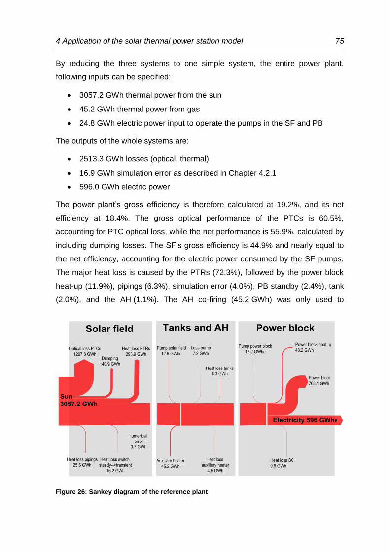
4 Application of the solar thermal power station model 75
By reducing the three systems to one simple system, the entire power plant,
following inputs can be specified:
3057.2 GWh thermal power from the sun
45.2 GWh thermal power from gas
24.8 GWh electric power input to operate the pumps in the SF and PB
The outputs of the whole systems are:
2513.3 GWh losses (optical, thermal)
16.9 GWh simulation error as described in Chapter 4.2.1
596.0 GWh electric power
The power plant’s gross efficiency is therefore calculated at 19.2%, and its net
efficiency at 18.4%. The gross optical performance of the PTCs is 60.5%,
accounting for PTC optical loss, while the net performance is 55.9%, calculated by
including dumping losses. The SF’s gross efficiency is 44.9% and nearly equal to
the net efficiency, accounting for the electric power consumed by the SF pumps.
The major heat loss is caused by the PTRs (72.3%), followed by the power block
heat-up (11.9%), pipings (6.3%), simulation error (4.0%), PB standby (2.4%), tank
(2.0%), and the AH (1.1%). The AH co-firing (45.2 GWh) was only used to
Figure 26: Sankey diagram of the reference plant

76 4 Application of the solar thermal power station model
maintain the SF’s temperature and is 3.3% of the SF thermal energy output. As
stated in Eq. (65), during PB standby mode, molten salt from the hot tank is used
to maintain the SG’s temperature. This causes 9.8 GWh of thermal losses. PB
heat-up consumes 48.2 GWh of thermal energy. In all, the PB operates at 6.9% in
off-design mode, resulting in a gross efficiency of 42.3% and net efficiency of
41.4% over the entire year. The PB electric output is 596 GWh. Further discussion
of the economic efficiency and the LECs is found in Chapters 4.5, 4.6, and 4.7.
4.3 Comparison of stationary and transient solar field model
In order to compare the transient and stationary SF simulation model, the
reference plant, described in Chapter 4.1, is modified. The value of the two
parameters and , listed in Appendix C, are changed from 1 to 0,
which signifies a quasi-stationary simulation. The instationary components IS1,
IS2, IS3, IS4, IS5, IS6, and IS7, shown in Figure 6, are therefore deactivated. All
other parameters are equal to the reference plant’s parameters. The additional
indirect storage component heat loss of 16.2GWh, described in Chapter 4.2.1, is
added in accordance with Eq. (83) to the PB electric output. Because the models’
system behavior differ, their AH heat inputs are not equal. The difference is
7.4 GWh. To compare the two simulations, they must have the same energy input,
so the reference energy of the AH ( =45 GWh) is introduced. The electric
output can therefore be calculated in a first approximation.
( ) (87)
Figure 27 shows the comparison of energy flows over the entire simulated year. In
this figure, the results of the reference plant energy flows, shown in Figure 26,
always refer to 100%. In order to describe the effects causing the two simulations’
differing results, one day has been chosen, shown in Figure 28. The hot and cold
tank temperatures, as well as the hot tank’s load level, are plotted over one day,
October 3, 2008, for the transient (continuous line) and the stationary (dashed line)
simulation. The temperature of the HTF at the SF outlet, which refers to the
temperature past component IS7 in Figure 6, is also plotted for both simulations.

4 Application of the solar thermal power station model 77
At 5:45, sunrise, both simulations are in start-up mode. Changes in the DNI
immediately result in changes in the SF’s outlet temperature in the steady
simulation. Because the sky is clouded for several hours on this day, which results
in high DNI changes, the red dashed SF temperature is discrete, whereas the
temperature course of the transient simulation is continuous. SF outlet
temperature changes, due to DNI changes, are delayed in the transient simulation
because the steel mass is heated, and the HTF’s velocity in the pipes is simulated.
At 15:05, both models simulate SF shut-down due to low radiation. This shut-down
process lasts 30 minutes, until the DNI is zero, in the steady simulation, and
340 minutes in the transient simulation. There are two reasons for this delay. First,
the hot HTF from the PTCs is delayed because its velocity in the pipes is reduced
during shut-down. Second the heat stored in the 1,789 metric tons of steel pipes is
transferred to the HTF. Because of the low mass flow, the heat transfer coefficient
is low, which results in a lower HTF temperature gradient than that present during
the start-up process. From 16:45 to 16:55, the skies clear, and low normal
radiation is plotted in Figure 28. This solar energy is collected by the transient
simulation PTCs, whereas the steady simulation is in night operations mode,
indicated by a focus factor in Eq. (11) of 0. This solar energy is therefore not
collected by the steady PTCs. Over the entire simulated year, this effect results in
0.20% reduced effective solar energy input, as shown in Figure 27.
A major effect is the reduced storage capacity of the steady simulation. Because
the headers and feeders are modelled exactly in the transient simulation, the
storage capacity is expanded by 1,789 metric tons of steel mass (
kJ/m³/K) and 3,115 metric tons of solar salt in the piping elements. Because
of the reduced storage capacity, more energy is dumped in the stationary
simulation during periods of high radiation. The PTCs are defocused for 16% of SF
operations in the steady simulation, whereas the PTCs of the transient simulation
are only defocused 15% of the time. This results in an additional 0.62% reduction
in energy input to the HTF, as shown in Figure 27.
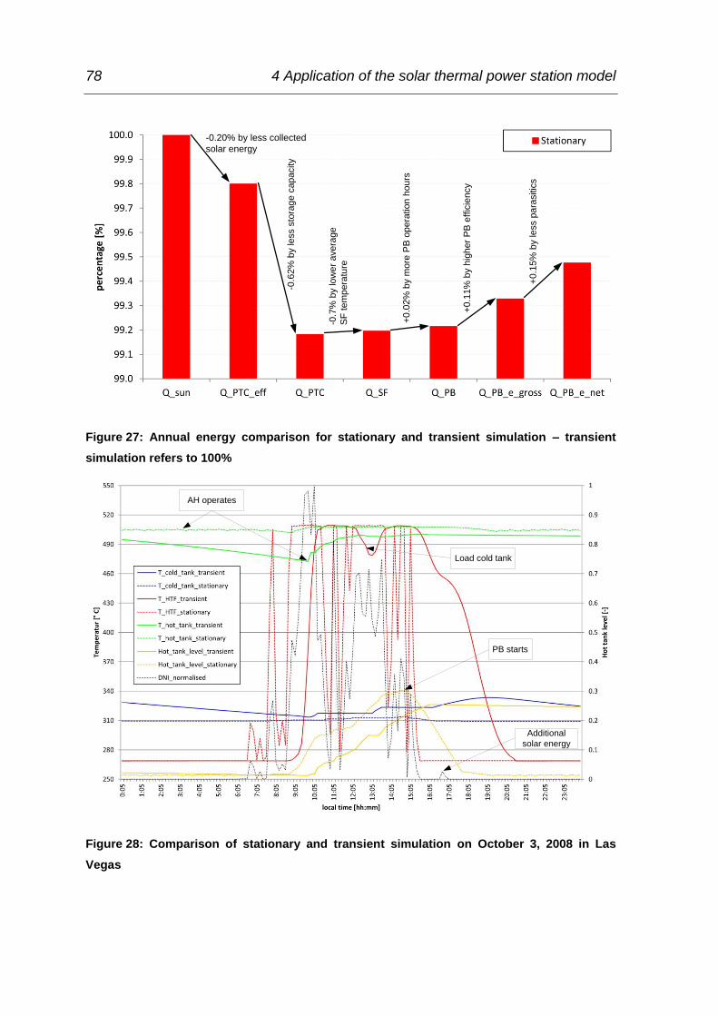
78 4 Application of the solar thermal power station model
Figure 27: Annual energy comparison for stationary and transient simulation – transient
simulation refers to 100%
Figure 28: Comparison of stationary and transient simulation on October 3, 2008 in Las
Vegas
-0.20% by less collected
solar energy
-0.6
2%
by le
ss s
tora
ge
ca
pa
city
-0.7
% b
y lo
we
r a
ve
rag
e
SF
te
mp
era
ture
+0
.02
% b
y m
ore
PB
op
era
tio
n h
ou
rs
+0.1
1%
by h
igh
er
PB
effic
ien
cy
+0.1
5%
by le
ss p
ara
sitic
s
Load cold tank
PB starts
Additional
solar energy
AH operates

4 Application of the solar thermal power station model 79
As previously stated, the start-up and shut-down processes are modelled in detail
in the transient simulation. During these processes, the hot HTF at the SF outlet is
pumped to the cold tank if its temperature is below 485 °C and to the hot tank if it
is above. This causes higher temperature gradients in the cold and hot tanks, as
shown in Figure 28. The annual average temperature of the hot tank is therefore
0.3% lower than that of the stationary simulation, whereas the temperature of the
cold tank is 0.8% higher. This difference in hot and cold tank temperatures has
three effects.
First, average SF temperature is higher because the cold tank temperature is
higher, which results in 0.7% higher SF heat loss in the transient simulation. The
annual energy out of the SF, calculated using Eq. (84), is therefore 0.02% higher
in the steady simulation, as shown in Figure 27.
Second, the annual PB efficiency is decreased because the annual mean
temperature of the hot tank is lower in the transient simulation. The annual PB
efficiency is 40.51% in the transient simulation and 40.61% in the steady
simulation. This causes a rise of 0.11% in the annual thermal input into the PB and
in the annual PB gross electric output, as shown in Figure 27.
Third, the SF parasitics are reduced by 5.84% in the steady simulation. According
to Eq. (3), the velocity of the HTF depends on a temperature rise through a PTC
loop. In the transient simulation, the annual mean rise is 194.2 °C, and in the
steady simulation it is 198.4 °C. HTF velocity is therefore lower in the steady
simulation, and as a result, the SF pumping parasitics are reduced. This causes a
rise of 0.15% to the annual gross and net electric output in Figure 27.
The PB operation hours for the two simulations are different. In the steady
simulation, the PB operates three days more than in the transient simulation. This
effect can be seen in Figure 28. At 14:45, the threshold level of 30% hot tank load
is reached in the steady simulation, and the PB starts to operate. In the transient
simulation, the 30% threshold level is not reached because more thermal energy is
stored in the cold tank. The energy stored in the hot and cold tanks is used to
maintain the SF outlet temperature. On the next day, the hot tank load is used to
feed the SG (not shown in Figure 28). But its heat capacity and temperature is

80 4 Application of the solar thermal power station model
reduced due to tank heat losses during the night. This causes a rise of 0.02% in
annual SF energy output and PB energy input in Figure 27.
Because the steady simulation model does not simulate start-up and shut-down, it
reflects 4.2% more thermal energy stored to the hot tank, and the AH is therefore
activated more often, which results in an increased heat input of 7.4 GWh, as
stated at the beginning of this chapter. During the morning hours, the AH is
activated every 35 minutes to produce hot HTF, as the dashed green line, the
temperature of the hot tank in the steady simulation, shows in Figure 28. The AH
is only activated at one time instant, 09:45, in the transient simulation, as indicated
in Figure 28.
4.4 Comparison of various time series time steps
In order to compare various time series time steps (TSs) in the time series dialog,
the reference plant, described in Chapter 4.1, is modified. The value of the
parameter , listed in Appendix C, is changed from 600 s to 900 s, 1800 s,
and 3600 s, which reflects to different TSs in the time series dialog. All other
parameters are equal to the reference plant’s parameters.
The Las Vegas solar data in one-minute resolution (527,040 data points) is
averaged to 10-, 15-, 30-, and 60-minute resolution in order that the annual
thermal input from the sun
( ) ∑
(88)
be equal for each TS ( ). The arithmetic mean DNI at a specific time step ( ) for
the four different TSs
( ( ))
∑
( )
[
[
(89)

4 Application of the solar thermal power station model 81
is calculated at the average TS (5, 7.5, 15, and 30 min). The arithmetic mean
ambient temperature at a specific time step ( ) is calculated using Eq. (89),
replacing the parameters to , and to .
Figure 29 shows the DNI discretization comparison for three different time steps
(10, 30, and 60 minutes), and the original DNI data (1 min.). The time between
sunrise at 06:53 and sunset at 16:34 is discretized in 10 time instants (60 min.
discretization), 19 time instants (30 min.), 38 time instants (15 min.), 58 time
instants (10 min.), and 582 time instants (original solar data). Generally, the
maximum number of time instants between sunrise and sunset can be calculated.
⌈ ⌉
(90)
The 60-minute discretisation in Figure 29 shows one time instant at 06:30 with an
arithmetic mean DNI, calculated with Eq. (89), higher than zero (0.025 W/m²). The
30-minute discretisation also has one time instant at 6:45 with a mean DNI higher
than zero (0.05 W/m²). These instants of time occur before sunrise, and this solar
Figure 29: DNI discretization comparison for three different TSs in Las Vegas on January 1,
2008
6:53 16:34
0
100
200
300
400
500
600
700
800
900
1000
05:30 06:30 07:30 08:30 09:30 10:30 11:30 12:30 13:30 14:30 15:30 16:30 17:30 18:30
DN
I [W
/m²]
local time [hh:mm]
1 min.
10 min.
30 min.
60 min.

82 4 Application of the solar thermal power station model
energy cannot be collected by the PTCs ( in Eq.(11)). Therefore the
integral of the DNI from sunrise to sunset in the 30- and 60-minute discretisation is
less than that in the original data. The probability that less energy is collected is
50% for each discretisation, and the energy loss
( ) (91)
can be calculated using the arithmetic mean DNI at the time instant before sunrise.
The same probability that less energy is collected also occurs after sunset. The
higher the discretisation, the higher the arithmetic mean DNI and TS, and the
higher the energy loss. The maximum discretisation error is shown in Figure 30 for
a summer day. No solar energy is collected during the time interval, which is
between zero minutes and
(92)
minutes. These instants of time ( ) are shown in Figure 30 for the
60-minute discretisation (04:57) and the 30-minute discretisation (04:42). The loss
Figure 30: Maximum 60- and 30-minute discretization error due to less collected solar
energy than the original 1-minute data, during a summer day
47.24
4.02 0
1
2
3
4
5
0
50
100
150
200
250
04:27 04:32 04:37 04:42 04:47 04:52 04:57
sun
he
igh
t [°
]
DN
I [W
/m²]
local time [hh:mm]
DNI
max time 60 min.
max time 30 min.
mean DNI 60 min.
mean DNI 30 min.
sun height

4 Application of the solar thermal power station model 83
can therefore be calculated using Eq. (91) to be 170 kJ/m² (60-minute
discretisation) and 7.2 kJ/m² (30-minute discretisation), which amounts to 0.5%
and 0.02%, of the total collected specific energy on this day, respectively. The
maximal inaccuracy of the 10- and 15-minute discretisation on this day is factually
zero because the DNI at 5 and 7.5 minutes after sunset, respectively, is nearly
zero.
In order to compare the results of the four simulations, the reference energy of the
AH ( =45 GWh) is introduced, as described in Chapter 4.3 and stated in
Eq. (87). The AH heat input is 40.7, 40.3, 38.9, and 23.57 GWh (10-, 15-, 30-, and
60- min. discretization).
Figure 31 shows the relative results of the annual energy comparison for the 10-,
15-, 30-, and 60-minute TS, where 100% reflects the reference plant results
(10-minute TS), shown in Figure 26. The absolute values are listed in Appendix O.
As stated in Eq. (88), the solar energy input is independent from the TS, and
therefore remains 100% in each of the four simulations. The effective energy input
to the PTCs (Q_PTC_eff), without taking dumping of solar energy into account, is
reduced due to the DNI discretisation error, shown in Figure 30, and the PTC
efficiency discretisation error, described in Appendix N. It is reduced by 0.03%,
0.13%, and 1.13% (15-, 30-, and 60-min. discretisation). Because the energy input
into the PTCs is calculated using the algebraic Eq. (11), no numerical inaccuracy,
as described in Chapter 4.2.1, can occur, and therefore the differences are
considered to be exact.
The light blue graph (Q_HT/Q_SF) in Figure 31 shows the ratio of annual SF
energy stored in the hot tank to the total annual SF output energy, calculated using
Eq. (85). The annual energy stored in the hot tank is also calculated with Eq. (85),
but totals only the energy flows into the hot tank. This ratio is 102.51% in the
reference plant, which means that the annual SF energy stored in the cold tank is
negative (-34.5 GWh). This results from the nighttime HTF recirculation over the
SF. The HTF is cooled by the piping element heat losses in the SF and stored
back in the cold tank. The ratio Q_HT/Q_SF falls with higher TSs, which means
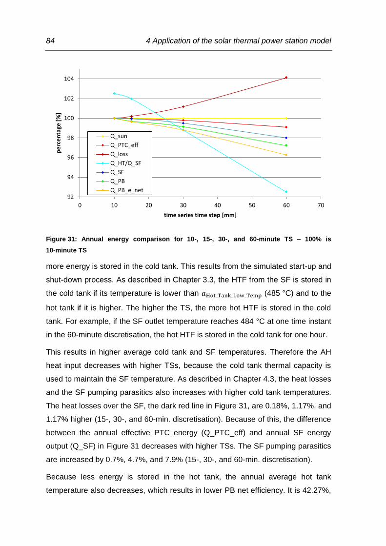
84 4 Application of the solar thermal power station model
more energy is stored in the cold tank. This results from the simulated start-up and
shut-down process. As described in Chapter 3.3, the HTF from the SF is stored in
the cold tank if its temperature is lower than (485 °C) and to the
hot tank if it is higher. The higher the TS, the more hot HTF is stored in the cold
tank. For example, if the SF outlet temperature reaches 484 °C at one time instant
in the 60-minute discretisation, the hot HTF is stored in the cold tank for one hour.
This results in higher average cold tank and SF temperatures. Therefore the AH
heat input decreases with higher TSs, because the cold tank thermal capacity is
used to maintain the SF temperature. As described in Chapter 4.3, the heat losses
and the SF pumping parasitics also increases with higher cold tank temperatures.
The heat losses over the SF, the dark red line in Figure 31, are 0.18%, 1.17%, and
1.17% higher (15-, 30-, and 60-min. discretisation). Because of this, the difference
between the annual effective PTC energy (Q_PTC_eff) and annual SF energy
output (Q_SF) in Figure 31 decreases with higher TSs. The SF pumping parasitics
are increased by 0.7%, 4.7%, and 7.9% (15-, 30-, and 60-min. discretisation).
Because less energy is stored in the hot tank, the annual average hot tank
temperature also decreases, which results in lower PB net efficiency. It is 42.27%,
Figure 31: Annual energy comparison for 10-, 15-, 30-, and 60-minute TS – 100% is
10-minute TS
92
94
96
98
100
102
104
0 10 20 30 40 50 60 70
pe
rce
nta
ge [
%]
time series time step [mm]
Q_sun
Q_PTC_eff
Q_loss
Q_HT/Q_SF
Q_SF
Q_PB
Q_PB_e_net

4 Application of the solar thermal power station model 85
42.25%, 42.19%, and 42.07% (10-, 15-, 30-, and 60-min. discretisation). It also
decreases because the pseudo-transient PB start-up process becomes longer with
higher TSs. The PB start-up process lasts about 50 minutes and cannot be
simulated properly using high TSs. Therefore the PB time in off-design is 6.9%,
7.3%, 8.1%, and 14.3% (10-, 15-, 30-, and 60-min. discretisation) and increases
with higher TSs. The increased SF parasitics, and the lower PB efficiency explain
the difference between annual PB heat input (Q_PB) and annual net electric
output (Q_PB_e_net) in Figure 31.
A difference between the blue line (Q_SF) and the green line (Q_PB) can also be
observed in Figure 31. This is because of the different PB operation hours. The PB
operates during 57.9%, 57.7%, 57.0%, and 56.1% (10-, 15-, 30-, and 60-min.
discretisation) of the total year, which results in 335, 333, 332, and 327 days (10-,
15-, 30-, and 60-min. discretisation) of operation. On bad days, described in
Chapter 3.3, the threshold level of the hot tank for PB operations is not reached
when high TSs are used. This causes lower PB operations hours, as described in
Chapter 4.3.
In all, the net electric output of the PB decreases with increasing TSs. It is
by -0.38%, -1.18%, and -3.75% (15-, 30-, and 60-minute discretisation) than that
of the reference plant’s electric output.
4.5 Comparison of three years with different direct normal
irradiation averaged annual sum
To compare three years with different direct normal irradiation averaged annual
sums, the reference plant, described in Chapter 4.1, is modified. The value of the
parameter , listed in Appendix C, is changed from 1, or Las Vegas, to 2, or
Almería. The latitude, longitude, and time zone of the sun element
(component 117), are therefore changed from 36.06°, -115.08°, and Pacific
Standard Time to 37.09°, 2.36°, and Central European Standard Time. All other
parameters remain equal to the reference plant’s parameters. The 2008 Las
Vegas DNI and ambient temperature in the time series dialog inputs are changed
to the 2010 and 2005 inputs, respectively. The direct normal irradiation averaged

86 4 Application of the solar thermal power station model
annual sum is 2095 kWh/m²/y in Almería during 2010, 2300 kWh/m²/y in Almería
during 2005, and 2659 kWh/m²/y in Las Vegas during 2008. Appendix M contains
further discussions of these locations.
In order to compare the results of the three simulations, the model introduces
reference AH energy ( =45 GWhth), as described in Chapter 4.3 and
calculated using Eq. (87). The AH heat input is 40.7, 48.0, and 48.1 GWh (Las
Vegas 2008, Almería 2005, and Almería 2010).
The economic and statistical model, as described in Chapter 3.4, is used to
calculate the LECs of the three simulations. The economic model input
parameters, and the employed distributions for those parameters, are listed in
Appendix L under “Economic parameters”. The design input parameters are the
thermal capacity of the storage (2,7436,049 kWhth), the aperture area (1.21 km²),
the total area of the plant (4.25 km²), and the design power block electric output
(125,000 kWhe). These parameters are similar for all three simulations. The result
of the simulation, the PB annual net electric output, is 572.0 MWh, 490.4 MWh,
and 447.0 MWh (Las Vegas 2008, Almería 2010, and Almería 2005). The Sankey
diagrams with the absolute energy flow values for the Almería 2010 and 2005
simulations can be found in Appendix P.
Figure 32 a) shows the pdf for the three simulations and for the improved power
plant, described in Chapter 4.6. Figure 32 b) shows the cdf for these simulations.
As stated in Eq. (78), the integral of the pdf results in the cdf. The mean value,
according to Eq. (79), is plotted as a dashed line in the corresponding colour for
the four simulations. The mode value is also indicated in both figures with a hash
key in the corresponding colour. The mean, mode, and median LEC value for each
simulation is not equal, as described in Chapter 3.4.2. The mean LEC result from
the mean input parameters ( , ,
, €/kWhe, 275 €/m², =35 €/m², 0.09, =25)
The maximum and minimum possible LECs, shown in Figure 32, are 0.09 to
0.23 €/kWhe (Las Vegas), 0.10 to 0.27 €/kWhe (Almería 2005), and 0.11 to
0.30 €/kWhe (Almería 2010).

4 Application of the solar thermal power station model 87
a)
b)
Figure 32: The a) probability density function and b) cumulative density function of the
LECs for Las Vegas 2008 (2659 kWh/m²/y), Almería 2005 (2300 kWh/m²/y) and 2010
(2095 kWh/m²/y), and the improved PP of Las Vegas 2008
0.148
0.176 0.193
0.151
0.149
0.172
0.190
0.143
0
2
4
6
8
10
12
14
16
18
0.09 0.12 0.15 0.18 0.21 0.24 0.27
Pro
bab
ility
de
nsi
ty f
un
ctio
n (
pd
f) [
-]
Levelized electric cost (LEC) [€/kWhe]
Las Vegas 2008meanAlmería 2005meanAlmería 2010meanLas Vegas 2008 impmean
0.148
0.176 0.193
0.151
0.149 0.172 0.190
0.143
0.00
0.10
0.20
0.30
0.40
0.50
0.60
0.70
0.80
0.90
1.00
0.09 0.12 0.15 0.18 0.21 0.24 0.27
cum
ula
tive
de
nsi
ty f
un
ctio
n (
cdf)
[-]
Levelized electric cost (LEC) [€/kWhe]
Las Vegas 2008meanAlmería 2005meanAlmería 2010meanLas Vegas 2008 impmean

88 4 Application of the solar thermal power station model
The range of probable LECs expands when the direct normal irradiation averaged
annual sum decreases, and is increased by 16.2% for Almería in 2005 and 28.9%
for Almería in 2010, compared to the reference plant’s results. The LEC forecast is
therefore less accurate, which results in a more uncertain financial situation for the
project.
Another disadvantage is the increased LECs. The median LEC is 0.150 €/kWhe
(Las Vegas 2008), 0.175 €/kWhe (Almería 2005), and 0.192 €/kWhe (Almería
2010). It is between the mode and mean LEC of the corresponding LEC
distribution. The probability that the LEC of the solar thermal power plant is less
than the median value is exactly 50%. With a 90% confidence interval (
), the LECs are between 0.117 and 0.190 €/kWhe (Las Vegas 2010), 0.136
and 0.221 €/kWhe (Almería 2005), and 0.149 and 0.243 €/kWhe (Almería 2010).
The mode LEC, which is most probable, is 0.149 €/kWhe (Las Vegas 2008),
0.172 €/kWhe (Almería 2005), and 0.190 €/kWhe (Almería 2010). The mode LEC is
increased by 13.3% (Almería 2005), and 23.8% (Almería 2010), whereas the
normal irradiation averaged annual sum is reduced by 13.5% (Almería 2005), and
21.2% (Almería 2010), compared to the reference plant’s results. The function
( ) is assumed to be an exponential function
( ) (93)
with the limits
( ) (94)
and
( ) (95)
where the mode LEC value of 0.080 €/kWhe refers to a solar thermal power plant
in which the PB operates for the entire year at 100% load. According to this
assumption, the calculated net electric output is 1050 GWh. The coefficients
(0.080), (6275), and (5.796) can therefore be calculated. The simulated
values for Las Vegas 2008, Almería 2005, and Almería 2010, as well as the
resulting function of Eq. (93), are plotted in Figure 33. The LECs can therefore be
estimated for other locations with direct normal irradiation averaged annual sums

4 Application of the solar thermal power station model 89
different from that of the reference plant, if the absolute latitude of the location is
comparable to Las Vegas’ (36.06°) or Almería’s absolute latitude (37.08°).
4.6 Improvement of the reference plant
The reference plant, described in Chapter 4.1, is modified to reduce its LECs of it
by changing a parameter in the user interface. After each change, the “Design
power plant script”, shown in Appendix F, generates a redesign of the power plant,
and a one-year re-simulation is run. Table 12 lists these improved parameters.
The Sankey diagram with the absolute values is found in Appendix P.
The hot tank’s temperature was set to 550 °C, which is considered to be the
maximum level for solar salt. The re-simulation therefore assumes a safety
clearance of 50 °C. The higher hot tank temperature results in a lower temperature
at the SG outlet, and a cold tank design temperature of 290 °C has therefore been
chosen. During start-up and shut-down, the HTF from the SF is pumped to the hot
tank if its temperature is higher than 450 °C. More energy is therefore stored in the
Figure 33: The LECs for Las Vegas 2008 (2659 kWh/m²/y), Almería 2005 (2300 kWh/m²/y) and
2010 (2095 kWh/m²/y), and the trend line of direct normal irradiation averaged annual sum
function to LECs
1,750
2,000
2,250
2,500
2,750
3,000
0.09 0.11 0.13 0.15 0.17 0.19 0.21 0.23 0.25 0.27
dir
ect
no
rmal
irra
dia
tio
n a
vera
ged
an
nu
al s
um
[k
Wh
/m²/
y]
Levelized electric cost (LEC) [€/kWhe]
mode LECs
trend
Las Vegas 2008
Almería 2005
Almería 2010

90 4 Application of the solar thermal power station model
hot tank and less in the cold tank. This results in lower SF pumping parasitics, less
SF heat loss, and more PB operation hours. The simulation reveals the
3/2 H layout to be the best, reducing SF pumping parasitics and heat losses. The
hot tank capacity is also expanded in order to realize 24-hour PB operation during
summer days.
Figure 34 shows the comparison of energy flows over the entire simulated year, in
which 100% always refer to the results of the reference plant energy flows, shown
in Figure 26. Because the solar multiple is decreased by 0.068, the net aperture
area of the SF is less, and the collected sun heat is therefore 3.37% less in the
improved plant. The overall gross efficiency of the PTCs, without taking solar
energy dumping into account, is equal to the reference plant’s efficiency. This
means that the relative solar heat input (Q_sun), and the effective PTC heat input
(Q_PTC_eff) remains constant (96.63%).
The net efficiency is higher because the storage is expanded in the improved
simulation, which results in less energy dumping during periods of high radiation.
Defocusing of PTCs is 71.3% less than in the reference power plant. This causes
a rise of 6.19% in annual net PTC heat input and annual gross PTC heat input
(Q_PTC), as shown in Figure 34.
The average SF temperature is higher, so heat losses in the piping elements are
also higher (+9.35%), which results in a reduced SF heat output (Q_SF). This
output is reduced by 1.59%, as reflected in the annual gross PTC heat input,
shown in Figure 34.
Table 12: Changed parameters of the reference plant
Parameter Reference plant Improved plant
Hot_Tank_Design_Temp 510 °C 550 °C
Hot_Tank_Low_Temp 485 °C 450 °C
Cold_Tank_Design_Temp 310 °C 290 °C
loops 2H layout 3/2H layout
SM 2.233 2.165
Storage_time 10 h 13 h

4 Application of the solar thermal power station model 91
Because of the expanded thermal storage system, the PTCs are defocused less,
and more energy is stored in the hot tank. The PB operation hours are therefore
expanded by 4.25%. During summer periods, 24-h PB operation is realized. As
shown in Figure 34, the heat input to the PB (Q_PB) is 1.98% higher than the heat
output by the SF. Because of the higher live steam temperature (540 °C) at the PB
design point, the efficiency increases to 45.1%. This results in a 1.99% higher
annual PB gross efficiency. The net electric output of the PB is therefore increased
by 2.05%, as measured by the relative change to the heat input into the PB in
Figure 34.
The net efficiency of the entire power plant increases because the pumping
parasitics are lower in the SF and PB. The pumping parasitics in the SF are
reduced due to the optimized layout and the lower cold tank temperature, which is
297.6 °C, 4.5% lower than that of the reference plant. The PB feed water mass
flow is also reduced by 6.7% at the design point, which results in lower annual PB
parasitics. In all, the annual net electric output of the PB increases by 6.3%,
whereas the total investment costs increase by 3.1% (based on the mean cost
input values listed in Appendix L under “Economic parameters”).
Figure 34: Annual energy comparison for the reference and improved solar thermal power
plant – reference plant refers to 100%
-3.3
7%
by le
ss a
pe
rtu
re a
rea
+6
.19
% b
y h
igh
er
sto
rag
e
ca
pa
city
-1.5
9%
by h
igh
er
ave
rag
e
S
F te
mp
era
ture
+1.9
8%
by m
ore
PB
o
pe
ratio
n h
ou
rs
+2.0
5%
by h
igh
er
P
B e
ffic
ien
cy
+1.1
1%
by le
ss
p
ara
sitic
s

92 4 Application of the solar thermal power station model
The resulting LEC pdf, and cdf is shown in Figure 33. The same economic and
statistical model, described in Chapter 4.5, is used to calculate these functions.
The input values in this model are PB net electric output (607.8 GWhe), AH
reference energy ( =45 GWhth), total power plant area (3.87 km²), aperture
area (1.15 km²), design gross PB capacity (125 MWe), and storage capacity
(3,888,112 kWhth). The mode LEC is reduced by 0.6 cents/kWhe, whereas the
mean LEC is reduced by 0.3 cents/kWhe. The distribution of probable LECs is
reduced by 3.5%, so the LEC forecast is more accurate for the improved power
plant. The 90% LEC confidence interval ( ) is between 0.114 and
0.184 €/kWhe. This interval is 4.1% lower than that of the reference plant.
4.7 Comparison of various cooling methods
In order to compare various PB cooling methods, the reference plant, described in
Chapter 4.1, is modified by changing the value of the parameter
, listed in Appendix C, from 0.08 bar to 0.25 bar and 0.5 bar.
The pressure of 0.25 bar reflects a hybrid cooling system, and the pressure of
0.5 bar reflects a dry cooling system (NREL 2009, p. 16). All other parameters
remain equal to those of the reference plant.
The reference plant annual PB net efficiency is 41.4%, and the net efficiency of the
entire solar thermal power plant is 18.4%. The PB net efficiency is plotted as a
continuous blue line in Figure 35. It is approximately 43.9% at full PB load, and
39.1% at 40% PB load. The red line corresponds to the net efficiency of the PB
with hybrid cooling system, and is 39.9% at full load and 35.6% at 40% load. The
PB with dry cooling system (green line) has a net efficiency of 37.5% at full load
and 33.1% at 40% load.
The ratio of the net PB efficiency with alternative cooling system ( ) to the net
efficiency of the reference plant ( )
(96)
is plotted in Figure 35. It decreases with PB load and can be fitted by the following
two functions.

4 Application of the solar thermal power station model 93
( ) (97)
( ) (98)
If the thermal input into the PB remains constant, the electrical output of the PB
with alternative cooling system at a specific time instant
( ) ( ( )
)
( ) (99)
is calculated using the factors from Eqs (97) and (98), the electric power at the
design point of the reference power plant ( ), and the electrical output of
the time instant ( ( )). Because the thermal power input into the PB is
assumed to be equal to the thermal power input in the reference plant simulation,
the results can be transferred to the PB with alternative cooling system without
influencing the reference SF system behavior. Adopting Eq. (99) for the reference
plant’s time series dialogue results yields, electrical net outputs of 538.7 GWh
(hybrid cooling) and 506.7 GWh (dry cooling). The electrical energy produced is
10.8% (hybrid), and 16.1% (wet) less than that of the reference plant. This result
matches the 5% to 20% efficiency penalties proposed by (California Energy
Commission 2002, p. 1-9).
Figure 35: PB efficiency to the PB load for two different cooling systems.
0
0.1
0.2
0.3
0.4
0.5
0.6
0.7
0.8
0.9
1
0.4 0.5 0.6 0.7 0.8 0.9 1
Effi
cie
ncy
[-]
load PB [-]
Net efficiency reference systemNet efficiency hybrid cooling systemNet efficiency dry cooling systemRatio dry cooling systemRatio hybrid cooling system

94 4 Application of the solar thermal power station model
To calculate the LECs, the simulation assumes an overall water reduction of 30%
and 70% (hybrid and dry cooling system, respectively). It also assumes that the
costs of the reference plant cooling system are 1% of the overall costs of the PB
and that a hybrid cooling system entails a 300% cost increase and a dry cooling
system a 900% increase. It assumes no differences in operating and maintenance
costs (California Energy Commission 2002, p.9-2ff).
Figure 36 shows the resulting LEC cdf for the three cooling systems. The mean
LEC value increases by 1 and 2 dent/kWhe, which translates to an increase of
6.6% (hybrid) and 13.2% (dry). The mode LEC increases by 0.7 and 1.9
Cent/kWhe, which translates to an increase of 4.7% (hybrid) and 12.8% (dry). The
cdf of hybrid and dry cooling system LEC values is also expanded by 5.6% and
11.3%, respectively, and the LEC forecast is therefore less accurate, resulting in
less certain project finance. Further discussion of the power plant’s cooling system
is found in Appendix Q.
Figure 36: The cumulative density function of the LECs for Las Vegas 2008 with wet cooling
system, hybrid cooling system, and dry cooling system
0.151
0.161
0.171
0.149
0.156
0.168
0.00
0.10
0.20
0.30
0.40
0.50
0.60
0.70
0.80
0.90
1.00
0.09 0.12 0.15 0.18 0.21 0.24 0.27
cum
ula
tive
de
nsi
ty f
un
ctio
n (
cdf)
[-]
Levelized electric cost (LEC) [€/kWhe]
Las Vegas 2008 (wet)meanhybridmeandrymean

5 Summary and Conclusion 95
5 Summary and Conclusion
In this thesis, a transient thermodynamic model of a solar thermal power station is
implemented into the commercial software tool EBSILON®Professional 10.01.01.
The solar field is modelled in transient mode using both the indirect storage
component and the direct storage component. The system behavior of the PB is
modelled in pseudo-transient mode by an EbsScirpt that estimates the PB thermal
inertia. A user interface allows up to 42 parameters to be specified to design an
individual solar thermal power plant, including design parameters, operation
strategy parameters, and simulation mode parameters.
Different choices of SF layout (I, H, 3/2, 2 H layout), PTC (EuroThrough 150,
HelioTrough, UltimateTrough), solar multiple, storage time, and AH capacity allow
the SF model to be individualized. Several SF pipe design parameters are also
available, e.g. wall thickness, design HTF velocity, and pipe wall roughness. A
ramp-up factor and start-up time can also be specified in the interface to model the
pseudo-transient behavior of the PB. The gross capacity of the power plant and
the turbine back-pressure can be specified.
The model uses plant operation management to identify the instant of time for PB,
AH, and SF start-up, all of which can also be specified in the user interface.
Simulation mode can be set to transient or steady simulation. Only start-up,
shut-down, and transient SF states during clouding can be simulated in transient
mode, which results in a simulation wall clock time of about 12 hours at a common
work station (one year with ten-minute resolution). The entire time between
start-up and shut-down, or the entire year, can also be simulated in transient
mode, which results in a very long simulation wall clock time (up to 10 times as
long).

96 5 Summary and Conclusion
The implementation of the solar thermal power station into the
EBSILON®Professional software was a “Husarenstück”, because several problems
occurred.
First, the instationary component 119 was introduced in the latest version, version
10, and is therefore new. The software uses only a second-order boundary
condition between the environment and the component, which is not suitable for
PTC simulation. A third boundary condition, simulating the specific heat input to
the component, would be more realistic.
The EbsScript function “transferAllResults” could not be used in the implemented
model because the component 119 matrix values (e.g. the temperatures in the
indirect storage component), could not be transferred to other Ebsilon profiles.
This Ebsilon bug prevented the use of Ebsilon profile selection, and an EbsScript
instead implemented the profile selection into the model. Various profiles must
therefore be implemented by a code instead of the Ebsilon graphical user
interface. If this bug were to be solved in the future, the standard Ebsilon profile
selection could be used to enable a more user-friendly implementation of new
profiles.
Another problem was that numeric controllers (Component 39 and 12) are only
able to operate during stationary simulations. During transient simulations, these
components cause errors. The “Forecast salt mass flow”, shown on the left side of
the screenshot in Appendix A, was therefore implemented. This model calculates
the SF mass flow for the next time instant, performing a steady simulation. This
result is used in the next time instant if a transient simulation is in progress.
Second, it was difficult to determine the numerical accuracy of the simulation. If
the simulation does not converge to the desired residuals of , the value of the
function “@calcoptions.res.status” is 3. However, the value of the function
“@calcoptions.sim.matprec” was always 3, indicating residuals of . Ebsilon
does not offer a tool for tracking numerical accuracy for simulations in the time
series dialog. Therefore the numerical accuracy was estimated, as described in
Chapter 4.2.1. The accuracy was identified as being between to , for the
simulation of the entire year.

5 Summary and Conclusion 97
In order to simulate the solar thermal power plant’s LECs, a stationary simulation
with a ten-minute discretization is proposed. For Las Vegas, the difference in the
net electric output between stationary and transient simulation is identified as
0.53%, which is relatively low. The simulation wall clock time is 50% lower than the
transient simulation. The transient simulation offers more realistic results,
wherefore a time resolution of less than 15 minutes is proposed.
The LECs were calculated for a reference plant for three different years with
different averaged direct normal irradiation annual sums (2095 kWh/m²/y,
2300 kWh/m²/y, and 2659 kWh/m²/y). The reference plant’s PB has a gross design
capacity of 125 MW, and its live steam parameters are 150 bar and 550 °C. The
solar field layout is assumed to be a 2 H layout with 352 collector loops, each
consisting of four Eurotrough ET150 collectors. The solar multiple is therefore
2.233. The storage time is 10 h.
Given the 90% confidence interval ( ), the LECs are between 0.117 and
0.190 €/kWhe (2659 kWh/m²/y), 0.136 and 0.221 €/kWhe (2300 kWh/m²/y), and
0.149 and 0.243 €/kWhe (2095 kWh/m²/y). The mode LECs are 0.149 €/kWhe,
0.172 €/kWhe, and 0.190 €/kWhe. An improved solar thermal power plant was
identified, so the mode LEC is reduced by 0.6 cents/kWhe. The 90% LEC
confidence interval is between 0.114 and 0.184 €/kWhe.
The economic impact of wet, hybrid, and dry PB cooling methods were also
compared. The mode LEC increased by 0.7 for hybrid cooling and 1.9 Cent/kWhe
for dry cooling.
The solar thermal power plant model offers much scope for parameter variation,
allowing further investigation. The designed solar thermal power plants can be
compared by using the implemented statistic and economic model to calculate the
LECs. Further investigations in the simulation mode (transient or steady), and
varying time series time steps are also possible.

98 5 Summary and Conclusion
Plant operation management strategy is kept as simple as possible. For example,
the auxiliary heater only operates when the temperature in the solar field is critical.
The model accounts for no SF or PB support during start-up. Plant operation
management could therefore be modelled in more detail in order to raise the
economic performance of the entire plant.

Appendix 99
Appendix
Appendix A: Screenshot of the Ebsilon model of the solar field

100 Appendix
Appendix B: Screenshot of the Ebsilon model of the power block

Appendix 101
Appendix C: User input parameters and output parameters for the
design process of the solar thermal power plant
User input parameters to design the solar field and the power block
Parameters for the design point of the SF
Location The location of the power plant
(Las Vegas, Almería or user-defined at sun
component), described in Chapter 3.1.2 and used
for the DNI-5034 algorithm
T_amb_design Temperature at design point of the solar thermal
power plant used for the Eq. (26) and (33)
DNI_design DNI at the design point of the solar thermal power
plant
Date_design Date at the design point of the solar thermal power
plant
Parameters for solar field layout
loops Layout of the solar field (I, H, 3/2 H and
2 H layout), described in Chapter 3.1.3
SM Solar multiple of the solar thermal power plant
PTC_type Type of parabolic trough collector, listed in
Appendix H and described in Chapters 2.2, 2.3
and 3.1.4
(EuroTrough + PTR 70, HelioTrough + PTR 90,
UltimateTrough + PTR 90, user-defined at parent
collector component)
PTC_loop Number of collectors in a loop (four, six, eight, or
ten), described in Chapter 3.1.3 and employed in
Eq. (10)
W_PP Width of balance of plant, described in Chapter
3.1.5 and employed in Eq. (19) and (20)
D_u_pipe Distance between two u-pipe elements for thermal
tension release, described in Chapter 3.1.5 and
employed in Eq. (23)

102 Appendix
S_u_pipe_f1 Side length of u-pipe for feeder 1, described in
Chapter 3.1.5 and employed in Eq. (24)
S_u_pipe_f2 Side length of u-pipe for feeder 2, described in
Chapter 3.1.5 and employed in Eq. (24)
S_u_pipe_h Average side length of u-pipe in header, described
in Chapter 3.1.5 and employed in Eq. (24)
Parameters for pipe design
Heat_losses_pipe Heat losses of all piping elements (except
parabolic trough receiver) and distributing and
collecting header, described in Chapter 3.1.5 and
employed in Eq. (26)
V_Design Design velocity for piping elements and headers,
described in Chapters 3.1.5, 3.1.8.2, and 3.1.8.3
and employed in Eq. (28), (44), (47), (52) and (53)
KS Pipe wall roughness for piping elements and
headers, described in Chapter 3.1.5 and employed
in Eq. (28)
Parameters for storage system described in Chapter 3.1.6
Storage_time Time electricity can be produced at 100% load of
power plant using only thermal capacity of storage,
described in Chapter 3.1.6 and employed in
Eq. (31)
Delta_T_tank Temperature drop of full hot storage tank over one
day, described in Chapter 3.1.6 and employed in
Eq. (33)
Hot_Tank_Design_Temp Design temperature of hot tank, described in
Chapter 3.1.6 and employed in Eq. (33)
Cold_Tank_Design_Temp Design temperature of cold tank
Parameters for auxiliary heater design
Load_AH Percentage of total gross capacity that only
auxiliary heater can produce, described in
Chapter 0

Appendix 103
Parameters for transient simulation
t_feeder Thickness of feeder and header pipes, described
in Chapters 3.1.8.2 and 3.1.8.3 and employed in
Eq. (51)
D_outer_PTR Outer diameter of parabolic trough receiver (must
only be defined if user-defined collector is used for
simulation)
Parameters for PB
Gross_capcity Gross capacity of power plant
P_turbine_pack_pressure Turbine pack pressure, described in Chapter 0
User input parameters for plant operation management
Simulation mode
ts_tsc Time step of time series calculation
Forecast_Timesteps Transient simulation mode, used in EbsScript in
Appendix G
“1” calculates whole day transient (slow), or whole
year transient (very slow, comment lines 508-528
in EbsScript Intelligence)
“2” calculates start-up, shut-down, and low-
clouding periods during day transient (fast)
Mode_SF Simulation mode of C unit, described in
Chapter 3.2.5
“1” Transient
“0” Quasi-stationary
Mode_H Simulation mode of F-H unit, described in
Chapter 3.2.5
“1” Transient
“0” Quasi-stationary
Pseudo-transient behavior of PB, described in Chapter 3.2.6
d_SMF_d_t Gradient of salt mass flow during power block start
up in kg/s/s employed in Eq. (67)
Delta_t_startup Time for PB start-up employed in Eq. (64)

104 Appendix
Parameters to identify the weather conditions of a day, described in Chapter 3.3
Min_DNI_PB Minimum DNI over one day to start-up power block
DNI_bad_day Maximum average DNI for bad day
DNI_very_good_day Minimum average DNI for very good day
Parameters to identify whether power block can operate, described in Chapter 3.3
Min_HT_Level_PB_OP Minimum hot tank level if power block is operating
Min_HT_Level_bad_day Minimum hot tank level for power block operations
for a bad day
Min_HT_Level_good_day Minimum hot tank level for power block operations
for a good day
Min_HT_Level_very_good_day Minimum hot tank level for power block operations
for a very good day
Min_HT_Level_Day_AH Minimum hot tank level for AH during day
Min_HT_Level_Night_AH Minimum hot tank level for AH during night
Parameters to identify whether solar field can operate, described in Chapter 3.3
Min_Salt_M Minimum salt mass flow for solar field operations
Further parameters for plant operation management, described in Chapter 3.3
Hot_Tank_Low_Temp Lowest temperature of hot tank
Salt_Low_Temp Lowest temperature of molten salt
Design output parameters
Parameters of the SF capacity
M_tank Total mass of hot and cold storage tanks
C_tank thermal capacity of hot tank
SM_real The real solar multiple after design process (exact
SM can normally never be achieved)
Salt mass flow at design point
SMF_PB_Design Salt mass flow into power block
SMF_SF_Design Salt mass flow into solar field
SMF_Aux_Design Salt mass flow into auxiliary heater
Geometric parameters of the SF
L_Feeder_1 Length of first feeder (with u-pipes) employed in
Eqs (26) and (28)

Appendix 105
L_Feeder_2 Length of second feeder (with u-pipes) employed
in Eqs (26) and (28)
Nbranch Number of header branches used in Eqs (47),
(49), (51) and (52)
L_Header Length of collecting and distributing header (with
u-pipes) employed in Eqs (25), (26), (29) and (30)
A Land use of entire power plant
W_O Length of entire power plant from west to east
N_S Length of entire power plant from north to south
Aperture_Area Total gross aperture area of collectors
Efficiency parameters
Gross_eff_SF Gross efficiency of solar field
Net_eff_SF Net efficiency of solar field
Gross_eff_PB Gross efficiency of PB
Net_eff_PB Net efficiency of PB
Gross_eff_PP Gross efficiency of power plant
Net_eff_PP Net efficiency of power plant

106 Appendix
Appendix D: The time series dialog in Ebsilon

Appendix 107
Appendix E: Input and output parameters in the time series dialog
Input parameters
At each iteration step
Date/Time Date and the time of current simulation
Sun.DNI Solar radiation
Sun.TAMB Dry bulb ambient temperature
At first Iteration step (boundary conditions)
Hot_tank.TSTO Temperature of hot tank
Cold_tank.TSTO Temperature of cold tank
Hot_tank.LEVACT Mass stored in hot tank
Cold_tank.LEVACT Mass stored in cold tank
Output parameters
Parameters for power plant management
I.Salt_M_Prediction Predicted salt mass flow predicted by forecast
collector loop
I.Solarfield_operation “0” if SF is unable to operate, “1” if SF is able to
operate
I.profile Selected profile for this time instant:
“1” refers to “Solar field / power block profile
(steady)”
“2” refers to “Solar field / - profile (steady)”
“3” ” refers to “ - / Power block - profile (steady)”
“4” refers to “- / - profile (steady)”
“5” refers to “- / - profile with Auxiliary Heater
(steady)”
“6” refers to “Solar field / power block profile
(transient)”
“7” refers to “Solar field / - profile (transient)”
“8” refers to “Solar field / - profile with Auxiliary
Heater (transient)”

108 Appendix
Parameters for transient simulation
I.transient_ts Number of time steps of transient simulation of
collector loop
I.transient_ts_2 Number of time steps of transient simulation of
collecting header and hot feeder pipelines
I.sim_mode Mode of simulation of C unit: “0” refers to steady
simulation, “1” to start-up procedure during morning,
and “2” to transient behavior because of clouding
during day or shut-down procedure at the end of the
day
I.sim_mode_2 Like I.sim_mode for the H-F unit
Parameters of storage system
I.Hot_Tank_Level Level of hot tank
I.Cold_Tank_Level Level of cold tank
I.Hot_tank.TSTO Temperature of hot tank
I.Cold_tank.TSTO Temperature of cold tank
Temperatures of the SF
H2._2.T Temperature at outlet of collecting header
IS_7._2.T Temperature at outlet of feeder 1
PTCs parameters
Focus.H Focus of all collectors (from 0 to 1)
Parameters of power block
S5._1.M Mass flow into power block
Power.Q Simulated electric power of power plant
Real Power Real electric power of power plant
I.Q_startup Thermal energy into power block
Thermal energy flow in solar thermal power plant
I.Q_PB Thermal power into steam generator
I.Q_Sun Thermal power of sun on net aperture area of
collectors
I.Q_PTC Thermal power that HTF absorbs
I.Q_SF Thermal power to HTF over entire solar field

Appendix 109
I.Q_PTR Thermal losses in collector
I.Q_Piping Thermal losses in pipings and headers
I.Q_tank Thermal losses of hot and cold tanks
I.Q_IS_F_H Positive if thermal power is transferred from HTF into
steel of the headers and feeders; negative if thermal
power is transferred in opposite direction
I.Q_IS_C Positive if thermal power is transferred from HTF into
steel of PTCs; negative if thermal power is
transferred in opposite direction
I.Q_pump_SF Thermal energy input into HTF by two submersion
pumps of SF
Parasitics of solar thermal power plant
I.Parasitics_PB Pumping parasitics of PB
I.Parasitics_SF Pumping parasitics of SF
I.Parasitics_AH Thermal energy consumed by auxiliary heater
I.Parasitics_Hot_tank Thermal power into cold tank by HTF from hot tank
Parameters of sun
Sun.RSHEIGHT Height of sun
Sun.RSAZIM Azimuth angle of sun
Sun.RPHIINC Incident angle of sun
Calculation results
@calcoptions.res.status Status of current simulation
“0” Successful
“1” Successful with warnings
“2” Maximum number of iterations reached
“3” Maximum number of iterations reached with
warnings
“4” Calculation error
“5” Error before calculation
“6” General error
@calcoptions.res.time Time needed for simulation of this time instant in
milliseconds

110 Appendix
@calcoptions.res.iter Iterations needed for simulation of this time instant
@calcoptions.sim.matprec Residuals of simulation
“3” correlates to
“2” correlates to
“1” correlates to
“0” correlates to
I.Check_simulation Status of simulation check
“0” no simulation check required
“1...99” Changed salt mass flow into solar field in
kg/s steps
“100” turned off instationary component IS7
“101” turned off instationary component IS6
“102” turned off instationary component IS5
“103” set salt mass flow into solar field to 0 kg/s
Intelligence.Check_tank Status of tank check
“” no tank check
“>0” Mass defect due to error à overcharge
deduced from cold tank

Appendix 111
Appendix F: Schematic of the EbsScript to design the power
plant
Start EbsScript
PTC_Type
Write EuroTrough parameters into
model
1
Write UltimateTrough parameters into
model
Write HelioTrough parameters into
model
Load predefined PTC parameter into
model
023
Solar field layout
Set multipliersCalculate Feeder 1
Feeder 2 := 0
Set multipliersCalculate Feeder 1
Feeder 2 := 0
Set multipliersFeeder 1 := 0Feeder 2 := 0
Set multipliersCalculate Feeder 1 Calculate Feeder 2
3/2 H LayoutH LayoutI Layout 2H Layout
Write user-defined parameters into the
simulation model
Design process of the power block
Set branches of the header and
calculate the solar multiple (SM)
Paramters logical?
yes
End EbsScript
no
Simulation successful?
yes
End EbsScriptno
Requested SM fullfilled?
Simulation successful?
End Ebsscript
nono
yes
Calculate real feeder and header length and write
back results to the model
Design of the collecting and
distributing header
Design of pressure drops and heat losses of piping
elements
Design of geometry and heat transfer
coefficients (alphas) of the indirect
storage
Simulation successful?
no
Design of the auxiliary heater
yes
Simulation successful?
Design of the storage tank
yesEnd EbsScript
Iterative Design process of the number of headers
Residuum <10^(-7)
yes
no
Iterative piping desing process
Find branch number with lowest
deviation between requested and
actual SM
yes
no

112 Appendix
Appendix G: Schematic of the EbsScript for plant operation
management, executed before each time instant of the time
series dialog
Start EbsScript
Are requested forecasts reached?
Get current row in time series dialog, total rows and requested rows for
forecast (row_r)
Simulation to forecast the salt
mass flow for actual row
row = 6
Norow := row +1
Set parameters for the forecast of the
salt mas flow
6<row<=(rows-row_r) row>(rows-row_r)
Get variables for plant operation
managment
Yesrow := 6
Manipulation of the current simulation
model
Simulation mode of the header and
feeders?
Profile selection for steady simulation of
the PTCssteadytransient
Set parameters for transient simulation of the header and
feeder
Simulation mode of the
PTCs?
Profile selection for transient simulation
of the PTCs
transient
Perform simulation in the
current active profile
steady
Transient simulation
necessary for next time step?
no
Reason?
yes
Start up procedure when the sun rises
in the morning
Reason 1
Shut down procedure at the end of the day or
because of insufficient radiation
Reason 2
Set simulation mode to transient
for the PTCs, header and feeders
Set parameters for transient simulation
of the PTCs
Errors occured?
Check and manipulate the
current simulation model
yes
Simulation mode of the header and
feeders?
no
Reset to the reference profile
steady
Write back results from simulation to
time seriesEnd EbsScript
Simulation mode of the
PTCs?
transient
transient
Transient simulation for
the header and feeders still necessary?
steady
Set simulation mode to steady for
the header and feeders
no
yes
Set simulation mode to steady for
the PTCs
Transient simulation for the PTCs still necessary?
no
yes
Forecast of the salt mass flow
to decide if the solar field is able
to operate in a certain time step
Simulate
Errors occured?
yes
no
Iterative check of the
simulation
Photo Caption
Profile selection
Change simulation mode
Simulate

Appendix 113
Appendix H: The parameters of the three implemented PTCs
Property
EuroTrough
ET150
+ PTR 70
HelioTrough
+ PTR 90
UltimateTrough
+ PTR 90
Geometric parameters
Outer diameter 0.07 m 0.09 m 0.09 m
Inner diameter 0.064a m 0.082a m 0.082a m
Focal length 1.71 m 1.861 m 1.951 m
Aperture width 5.77 m 6.78 m 7.5 m
Length 148.5 m 191 m 242 m
Radial distance 17.28 m 20.922 m 23.22 m
Net aperture area 817.5 m² 1263 m² 1689 m²
Pipe wall roughness m m m
Optical Parameters
Optical efficiency 76.8% 81a% 80a%
Cleanliness factor 98% 98% 98%
Incident angle modifier3 ( ( ))
Heat losses3
a assumption 1 assumption based on √ 2 assumption based on
3 because no data is available in literature, parameters are adapted to all three PTCs

114 Appendix
Appendix I: T-S diagram of the designed power block
Eva
SH
RH
Eco
PH
1
PH
2
PH
3
D
PH
4
PH
5
C
HP
S1
HP
S2
LP
S1
LP
S3
LP
S2
LP
S4
LP
S5
Ste
am
extra
ctio
n 1
Ste
am
extra
ctio
n 2
Ste
am
extra
ctio
n 3
Ste
am
extra
ctio
n 4
Ste
am
extra
ctio
n 5
Ste
am
extra
ctio
n 6
AC
1
AC
2
AC
3
AC
4
AC
5

Appendix 115
Appendix J: Schematic of the profile selection implemented in
EbsScript
Sola
r fi
eld
/ p
ow
er
blo
ck p
rofi
le (
stea
dy)
Sola
r fi
eld
/ -
pro
file
(s
tead
y)-
/ P
ow
er b
lock
-
pro
file
(st
ead
y)-
/ -
pro
file
(st
ead
y)-
/ -
pro
file
wit
h
Au
xilia
ry H
eate
r (s
tead
y)
Sola
r fi
eld
/ p
ow
er
blo
ck p
rofi
le
(tra
nsi
ent)
Sola
r fi
eld
/ -
pro
file
(t
ran
sien
t)
Sola
r fi
eld
/ -
pro
file
w
ith
Au
xilia
ry H
eate
r (t
ran
sien
t)
Star
tP
rofi
le s
elec
tio
n
Sim
ula
tio
n
mo
de
of
the
PTC
s?D
ayti
me?
Day
tim
e?tr
ansi
ent
stea
dy
Ho
t ta
nk
leve
l?H
ot
tan
k le
vel?
Ho
t ta
nk
leve
l?C
an s
ola
r fi
eld
o
per
ate?
nig
ht
day
nig
ht
day
Ho
t ta
nk
leve
l?H
ot
tan
k le
vel?
no
yes
>Min
<Min
_AH
_day
>Min
_AH
_day
and
<M
in
>Min
<Min
_AH
_day
<Min
_AH
_nig
ht
>Min
>Min
_AH
_nig
ht
and
<M
in
>Min
>Min
<Min
_AH
_nig
ht
>Min
_AH
_day
and
<M
in>M
in_A
H_d
ayan
d <
Min
>Min
_AH
_nig
ht
and
<M
in
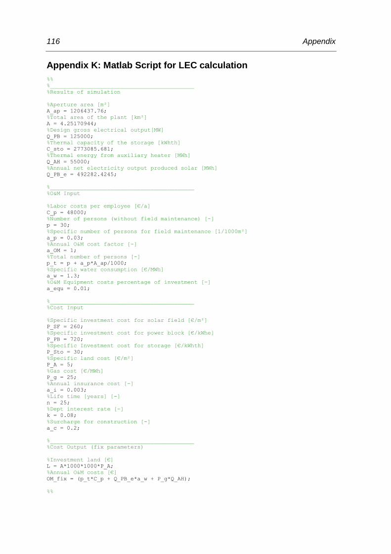
116 Appendix
Appendix K: Matlab Script for LEC calculation
%%
%___________________________________________
%Results of simulation
%Aperture area [m²]
A_ap = 1206437.76;
%Total area of the plant [km²]
A = 4.25170944;
%Design gross electrical output[MW]
Q_PB = 125000;
%Thermal capacity of the storage [kWhth]
C_sto = 2773085.681;
%Thermal energy from auxiliary heater [MWh]
Q_AH = 55000;
%Annual net electricity output produced solar [MWh]
Q_PB_e = 492282.4245;
%___________________________________________
%O&M Input
%Labor costs per employee [€/a]
C_p = 48000;
%Number of persons (without field maintenance) [-]
p = 30;
%Specific number of persons for field maintenance [1/1000m²]
a_p = 0.03;
%Annual O&M cost factor [-]
a_OM = 1;
%Total number of persons [-]
p_t = p + a_p*A_ap/1000;
%Specific water consumption [€/MWh]
a_w = 1.3;
%O&M Equipment costs percentage of investment [-]
a_equ = 0.01;
%___________________________________________
%Cost Input
%Specific investment cost for solar field [€/m²]
P_SF = 260;
%Specific investment cost for power block [€/kWhe]
P_PB = 720;
%Specific Investment cost for storage [€/kWhth]
P_Sto = 30;
%Specific land cost [€/m²]
P_A = 5;
%Gas cost [€/MWh]
P_g = 25;
%Annual insurance cost [-]
a_i = 0.003;
%Life time [years] [-]
n = 25;
%Dept interest rate [-]
k = 0.08;
%Surcharge for construction [-]
a_c = 0.2;
%___________________________________________
%Cost Output (fix parameters)
%Investment land [€]
L = A*1000*1000*P_A;
%Annual O&M costs [€]
OM_fix = (p_t*C_p + Q_PB_e*a_w + P_g*Q_AH);
%%

Appendix 117
%___________________________________________
%Monte Carlo simulation
%number of iterations
i= 1000000;
%Initialise vector for LECs
LEC = zeros( 1,i);
%res = zeros(1,i);
%i iterations to calculate LEC
for j=1:i
%normal distributed
P_PB = 720 + 72*randn/2.576;
%equally distributed
n = 20 + (30-20)*rand(1);
k = 0.06 + (0.12-0.06)*rand(1);
P_SF = 220 + (350-220)*rand(1);
P_Sto = 30 + (40-30)*rand(1);
a_c = 0.2 + (0.3-0.2)*rand(1);
a_equ = 0.005 + (0.02-0.005)*rand(1);
a_i = 0.002 + (0.004-0.002)*rand(1);
%calculate Data
CRF = (k * (1+k)^n) / ( (1+k)^n -1);
SF = P_SF*A_ap;
PB = P_PB*Q_PB;
ST = P_Sto*C_sto;
I = (1+a_c)*(L+ST+PB+SF);
OM = OM_fix + a_equ*I;
LEC(j) = (I*(CRF+a_i) + OM)/(Q_PB_e*1000);
%Calculate residuals
%{
for k=3:j
res(j) = res(j)+LEC(k);
end
res(j)=res(j)/(k-3);
res(j-2)=res(j-1)-res(j);
%}
end
%%
%%___________________________________________
%Plot result of LEC calculation
%Calculate mean LEC
mean_LEC = mean(LEC);
%Calculate mode LEC
x=min(LEC):0.001:max(LEC);
y = ksdensity(LEC,x);
[val, row] = max(y);
LEC_most_probable = x(row);
%comulative density function (cdf)
y = ksdensity(LEC,x,'function','cdf');
%plot function
plot(x,y, 'r','LineWidth',2);
xlabel('LEC [€/kWhe]');
ylabel('comulative density function (cdf) [-]');
axis([min(LEC) max(LEC) 0 max(y)]);
legend('comulative density function (cdf)','location','NorthWest');

118 Appendix
Appendix L: Parameters of the reference solar thermal power
plant
Parameters of the simulation
Residuals
Maximum iterations 500
Calculation mode Off-design
Time step (Comp 119) 10 s
Frequency of instationary
calculations (Comp 119)
At every 2nd iteration step
User input parameters to design the solar field and the power block
Parameters for the design point of the SF
Location Las Vegas
T_amb_design 30 °C
DNI_design 850 W/m²
Date_design 21.06.2010
Parameters for solar field layout
loops 8
SM 2.2
PTC_type EuroTrough + PTR 70
PTC_loop 4
W_PP 150 m
D_u_pipe 50 m
S_u_pipe_f1 10 m
S_u_pipe_f2 9 m
S_u_pipe_h 6 m
Parameters for pipe design
Heat_losses_pipe 200 W/m²
V_Design 2.5 m/s
KS 0.1 mm
Parameters for the storage system used in Chapter 3.1.6
Storage_time 10 h

Appendix 119
Delta_T_tank 1.1 K
Hot_Tank_Design_Temp 510 °C
Cold_Tank_Design_Temp 310 °C
Parameters to design the auxiliary heater
Load_AH 0.3
Parameters for the transient simulation
t_feeder 71 mm
Parameters for the PB
Gross_capcity 125 MW
P_turbine_pack_pressure 0.08 bar
User input parameters for plant operation management
Simulation mode
ts_tsc 600 s
Forecast_Timesteps 2
Mode_SF 1
Mode_H 1
Pseudo-transient behavior of the PB, described in Chapter 3.2.6
d_SMF_d_t 0.166 kg/s/s
Delta_t_startup 0.5 h
Parameters to identify the weather conditions of a day, described in Chapter 3.3
Min_DNI_PB 300 W/m²
DNI_bad_day 500 W/m²
DNI_very_good_day 800 W/m²
Parameters to identify whether power block can operate, described in Chapter 3.3
Min_HT_Level_PB_OP 0.04
Min_HT_Level_bad_day 0.3
Min_HT_Level_good_day 0.1
Min_HT_Level_very_good_day 0.04
Min_HT_Level_Day_AH 0.013
Min_HT_Level_Night_AH 0.013
Parameters to identify whether solar field can operate, described in Chapter 3.3
Min_Salt_M 150 kg/s

120 Appendix
Further parameters for plant operation management, described in Chapter 3.3
Hot_Tank_Low_Temp 485 °C
Salt_Low_Temp 270 °C
Design output parameters
Parameters of the SF capacity
M_tank 33,555 t
C_tank 2,7436,049 kWh
SM_real 2.233
Salt mass flow in design point
SMF_PB_Design 914 kg/s
SMF_SF_Design 2,180 kg/s
SMF_Aux_Design 253 kg/s
Geometric parameters of the SF
L_Feeder_1 537 m
L_Feeder_2 928 m
Nbranch 22
L_Header 893 m
A 4.25 km²
W_O 1,520 m
N_S 2,796 m
Aperture_Area 1.21 km²
Efficiency parameters (at design point)
Gross_eff_SF 67.204 %
Net_eff_SF 67.198 %
Gross_eff_PB 44.251 %
Net_eff_PB 43.862 %
Gross_eff_PP 29.738 %
Net_eff_PP 29.474 %
Pressure drops in the piping elements
P1 0.842 bar
P2 1.962 bar
H1 6.478 bar

Appendix 121
C1 0.495 bar
C2 0.472 bar
C3 0.459 bar
C4 0.455 bar
P3 0.5 bar
H2 5.539 bar
P4 1.830 bar
P5 0.786 bar
Heat transfer coefficients in indirect storages
IS1 2,245 W/m²/K
IS2 2,500 W/m²/K
IS3 2,684 W/m²/K
IS4 2,812 W/m²/K
IS5 3,718 W/m²/K
IS6 3,414 W/m²/K
IS7 3,133 W/m²/K
Discretization of indirect storages (X, Y)
IS1, IS2, IS3, IS4 (10, 1)
IS5 (15, 1)
IS6 (20,1)
IS7 (20,1)
Steel masses in indirect storages
IS1, IS2, IS3, IS4 (sum) 3 t
IS5 44.569 t
IS6 66.874 t
IS7 54.443 t
Total 1,789 t
HTF masses in indirect storages
IS1, IS2, IS3, IS4 (sum) 3.648 t
IS5 55.231 t
IS6 220.012 t
IS7 254.638 t

122 Appendix
Total 3,115 t
Heat transfer coefficients in steam generator
Eco
Primary 8,650 W/m²/K
Secondary 2,100 W/m²/K
Eva
Primary 49,100 W/m²/K
Secondary 2,400 W/m²/K
SH, RH
Primary 3,750 W/m²/K
Secondary 2,775 W/m²/K
Heat transfer areas in steam generator
Eco 1,322 m²
Eva 1,145 m²
SH 1,243 m²
RH 3,045 m²
Economical parameters (Matlab script shown in Appendix K)
25 €/MWhth
0.002-0.004 (uniformly distributed)
30
0.030 1/1000 m²
48,000 €/a
1.30 €/MWhel
0.005 – 0.02 (uniformly distributed)
0.2 – 0.3 (uniformly distributed)
720 €/kWhel (normally distributed – 99% of
values within 72 €/kWhel)
200 - 350 €/m² (uniformly distributed)
30 – 40 €/kWhth (uniformly distributed)
5 €/m²
0.06 – 0.12(uniformly distributed)
20 - 30 (uniformly distributed)

Appendix 123
Appendix M: The location used for the simulation of the solar
thermal power plant
The following criteria are defined for the location’s weather data set:
Direct normal irradiation averaged annual sum at least 2000 kWh/m²/y
Availability of solar data, especially for direct normal irradiation and dry bulb
temperature of at least ten minutes’ resolution over one year
Almaría in Spain and Las Vegas in the United States of America fulfil these
criteria, as detailed in the following section.
Figure 37 shows the worldwide annual direct normal irradiation in kWh/m²/y. The
two selected locations are indicated on the map. Almería is located in an area with
annual direct normal irradiation of between 2001 to 2200 kWh/m²/y, Las Vegas
between 2401 to 2600 kWh/m²/y. Solar data for Las Vegas is provided by the
NREL in one-minute resolution for the years 2007 to 2011 (NREL 2012), for
Almería by the DLR in ten-minute resolution for the years 2001 to 2011.
Figure 38 shows a plot of the annual direct normal irradiation of Almería and Las
Vegas. The average annual direct normal irradiation of Almería between 2002 and
Figure 37: Worldwide annual direct normal irradiation in kWh/m²/y from NASA SSE 6.0
adapted from (Trieb 2009)
Las Vegas Almería

124 Appendix
2011 is 2141.4 kWh/m²/y. In Las Vegas, the average is 2578.6 kWh/m²/y. To
investigate the influence of various direct normal irradiation averaged annual
sums, three years within the following DNI classes at these two locations are
selected:
Class 1: 2000 – 2100 kWh/m²/y à Almería (2010): 2095 kWh/m²/y
Class 4: 2300 – 2400 kWh/m²/y à Almería (2005): 2300 kWh/m²/y
Class 7: 2600 – 2700 kWh/m²/y à Las Vegas (2008): 2659 kWh/m²/y
A total of 25,729,646 km² of potential global sites for solar thermal power stations
with average annual direct normal irradiation exceeding 2000 kWh/m²/y exist
worldwide. However, only 25.5% of this area has irradiation higher than
2600 kWh/m²/y (Trieb 2009), much of it located in Africa, Australia, and the Middle
East, as Figure 37 shows. This means that the 2010 Almería yield analysis results
in correspond to a much larger area than those of the 2008 Las Vegas simulation.
The observation stations in Las Vegas (36.06°) and Almería (37.08°) lie on roughly
the same geographical latitude in the northern hemisphere. Nevertheless, the two
locations have different climates – Almería is Csa (warm temperate climate with
dry and hot summer, also known as Mediterranean climate) and Las Vegas BWh
(hot, arid desert climate) in the Köppen climate classification (Kottek 2006).
Figure 38: Annual direct normal irradiation for Almería from 2002 to 2011 and Las Vegas
from 2007 to 2011
22
30
20
99
20
48
23
00
19
52
21
41
21
43
22
36
20
95
21
70
24
65
26
59
25
37
25
65
26
67
0
500
1000
1500
2000
2500
3000
2002 2003 2004 2005 2006 2007 2008 2009 2010 2011
year
Almería
Las Vegas
Average: 2578,6
Average: 2141,4
An
nu
al d
ire
ct n
orm
al ir
rad
iati
on
[kW
h/m
²/y]

Appendix 125
Table 13 shows the weather data (maximum, minimum, and average temperature
and direct normal intensity) for the years 2005 and 2010 in Almería, and 2008 in
Las Vegas. The annual average temperature in Las Vegas is almost 22 °C, more
than 5 °C higher than in Almería. High ambient temperature causes lower thermal
losses from pipes and storages.
Figure 39 and Figure 40 show the temperature course of 2010 in Almería and
2008 in Las Vegas. The x-axis shows the number of days and the y-axis the local
time. A comparison of the two reveals that summer days in Las Vegas are hotter
than those in Almería, and the temperature drop at night is lower. Lowest
Table 13: Maximum, minimum, and average weather data for the year 2010 in Almería and
2008 in Las Vegas
Location year DNI [W/m²] Temperature [ °C]
max min average max min average
Almaría 2005 1077 0 263 40.8 -4.1 16.3
2010 1033 0 239 41.7 -3.9 16.5
Las Vegas 2008 1026 0 302 44.2 -1.4 21.8
Figure 39: Temperature progress in Almería during 2010
Figure 40: Temperature progress in Las Vegas during 2008

126 Appendix
temperatures are always reached in the hour after sunrise. During June, July, and
August, the temperature never falls below 18 °C in Las Vegas, while it drops as
low as 12 °C in Almería. The average temperature in the two regions during the
months of December, January, and February is comparable – 9.6 °C in Almería
and 9.7 °C in Las Vegas. Almería suffers the lowest temperatures (-4 °C).
Figure 41 and Figure 42 show the course of the direct normal radiance of 2008 in
Las Vegas and 2010 in Almería. During 2008, Las Vegas had only six days of
maximal direct normal irradiance of less than 300 W/m², whereas Almería had 22
during 2010. These days appear in the figures as blue vertical lines. During such
days, the PB cannot operate because the SF is unable to start-up. Figure 41 also
shows many more blue dots and lines during daytime in Almería, which indicates
clouding – in fact, direct normal irradiance remained below the 300 W/m² threshold
for 38 % of daytime. In Figure 42, the blue area during daytime is smaller – Las
Vegas fell below the threshold for only 24 % of daytime.
Figure 41: Direct normal radiance progress in Almería during 2010
Figure 42: Direct normal radiance progress in Las Vegas during 2008

Appendix 127
Appendix N: Effect of the time discretization on the PTC
efficiency
As described in Chapter 4.4, the effective heat input into the PTCs falls with larger
time series time steps (TSs) by 0.03%, 0.13%, to 1.13% (15-, 30-, 60- minute
discretization). The effect of the direct normal irradiation discretization error is
outlined in Chapter 4.4. This appendix outlines the discretization error of the PTC
efficiency, which is also increased by higher TSs.
Figure 43 a) shows the PTC efficiency during 2008 in Las Vegas. Highest
efficiency (as high as 75.3%) is achieved during June. During December,
efficiency reaches only 54.6%. Three days have been chosen: the summer
solstices in the northern hemisphere (June 21) and in the southern hemisphere
Figure 43: PTC efficiency a) over one year, and b) over three selected days (21.06, 21.09,
21.12)
day of year [ddd]
PS
T [
hh:m
m]
50 100 150 200 250 300 35000:00
02:00
04:00
06:00
08:00
10:00
12:00
14:00
16:00
18:00
20:00
22:00
24:00
0
0.1
0.2
0.3
0.4
0.5
0.6
0.721.06 21.09 21.12
discretet
21.06
21.12
21.09
b)
a)

128 Appendix
(December 21), and September 21. These days are shown in Figure 43 b). The
10-minute discretization is marked red, the 60-minute discretization blue.
The 60-minute discretization error on these days is -0.32%, -1.29%, and -0.46%
(June 21, September 21, and December 21), and +0.011%, -0.017%, and
+0.028% (June 21, September 21, and December 21) for the 10-minute
discretization, compared to the integral of the PTC efficiency over one day,
calculated with a one-second discretization (the yellow line in Figure 43 b)). The
discretization error on these days is nearly zero with the 10-minute discretization
and the simulation can therefore be assumed to be exact. The main PTC
efficiency discretization error with the 60-minute discretization is located next to
the two discrete points in the efficiency plot. These points are at 08:23 and 14:53
(December 21), 07:06 and 16:01 (September 21), and 6:09 and 17:13 (June 21).
To investigate the PTC efficiency discretization error in detail, the efficiency plot of
December 21 is fitted by two fifth-order polynomal functions. One function reflects
the PTC efficiency between sunrise and the first discrete point (08:23), and the
second from this discrete point to the local minima at 11:38. The rest of the day
from this minima to sunset is calculated by reflecting the two functions on the
y-axis.
A Monte Carlo simulation is performed, as explained in Chapter 3.4.2. The input
value of the Monte Carlo simulation is the first discretization time instant
(100)
that is varied between the minimum value ( = ), and the maximum value
( ). The output of the Monte Carlo simulation is the PTC
efficiency integral over the whole day, and the mean value of the PTC efficiency.
According to the central limit theorem, stated in Eq.(79), the mean value of the
PTC efficiency must be asymptotic given an infinite number ( ) of simulations
and independent of the discretization of time. The number of simulations has been
chosen to reach a residual of the mean efficiency of in order to calculate the
resultung cdf. The desired residuals were reached within 100 (1 minute), 1,000
(10-minute discretization), up to 1,000,000 iterations (60-minute discretization). In
all, the convergence is slower with increasing discretization of time. The resulting

Appendix 129
cdf of this simulation for the 1-minute (yellow line), 10-minute (orange line),
15-minute (green line), 30-minute (blue line), and 60-minute (red line)
discretizations is shown in Figure 44. The distribution of the 1-minute discretization
is not visible in this diagram resolution, so it can be assumed to be the mean
efficiency value.
The probability of underestimating the PTC collector efficiency is 53.5%
(60-minute resolution), 20.0% (30-minute resolution), 38.8% (15-minute
resolution), and 50.3% (10-minute resolution). On this day, the 30-minute
discretization has the highest probability of overestimating the collector efficiency,
whereas the 60-minute discretization has the lowest. This is the results of the time
difference between the first indiscrete point at 08:23 and the second at 14:53,
which is exactly 6.5 hours. This time difference is divisible by the 10-, 15-, and 30-,
but not by the 60-minute discretization. The possibility of overestimating the PTC
efficiency is therefore higher for the 10-, 15-, and 30-minute discretizations. If one
discretization point is exactly on or near the discrete point in the efficiency
function, another point of discretization is also on or near the other discrete point.
This results in an overestimation of the PTC efficiency. Therefore many calculated
PTC efficiencies are overestimated, which can be seen in the nearly vertical steps
in the cdfs of the 10-, 15-, and 30-minute discretization.
Figure 44: CDF for the PTC efficiency integral over the day of December 21 – efficiency is
discretized in 1-, 10-, 30-, and 60-minute resolution
201.78 0
0.1
0.2
0.3
0.4
0.5
0.6
0.7
0.8
0.9
1
200.7 201 201.3 201.6 201.9 202.2 202.5 202.8
com
ula
tive
de
nsi
ty f
un
ctio
n [
-]
Integral of efficiency [min]
1 minute
10 Minute
15 Minute
30 Minute
60 minutes

130 Appendix
Figure 43 introduces the time interval between the discrete point of June 21 and
September 21. High probability of PTC efficiency overestimation is therefore given
for a maximum of
⌈ ⌉
(101)
times during the entire year. The time interval is 130 minutes in the 2008
Las Vegas simulation. A high probability of PTC efficiency is therefore given for
13-14 times, 8-9 times, 3-4 times, and 1-2 times (10-, 15-, 20-, 30-, and 60-minute
discretization) over the entire year. The probability that the maximum number of
PTC efficiency overestimations from Eq.(101) will occur increases as the time
| | (102)
decreases. This time is 0, 5, 10, and 10 minutes (10-, 15-, 30-, and 60-minute
discretization), but at most , and therefore increased by higher TSs.
Even without exact mathematical proof, it can be stated that there is a tendency
for the solar heat input into the PTC to decrease with increased TSs. As stated in
Chapter 4.4, heat input is decreased by the DNI discretization error. Secondly, the
probability of overestimating PTC efficiency is lower with higher TSs. The
convergence to the real mean PTC efficiency is also slower with higher TSs.
Residuals of were not reached within 365 simulations for the examined day,
December 21.

Appendix 131
Appendix O: Absolute value comparison of for 10-, 15-, 30-, and
60-minute time series time step
Value 10 minutes 15 minutes 30 minutes 60 minutes
Annual energy flows [GWhth]
Q_sun 3057.2 3057.2 3057.2 3057.2
Q_PTC_eff 1849.5 1848.9 1845.7 1832.6
Q_loss 327.8 328.4 331.6 341.3
Q_HT 1406.7 1394.1 1338.5 1246.4
Q_CT -34.5 -27.0 15.9 100.8
Q_SF 1372.2 1367.0 1354.5 1347.2
Q_PB 1415.5 1411.3 1403.5 1376.4
Q_PB_e_gross 598.4 596.3 592.2 579.1
Q_PB_e_net 573.4 571.3 566.7 551.9
Efficiency [-]
PTC_eff 60.50 60.47 60.37 59.94
SF_gross 44.88 44.71 44.30 44.07
PB_gross 42.27 42.25 42.19 42.07
PB_net 40.51 40.48 40.38 40.10
PP_gross 19.57 19.50 19.37 18.94
PP_net 18.76 18.69 18.54 18.05
Parasitics [GWhe]
PB 12.2 12.2 12.0 11.7
SF 12.6 12.7 13.2 13.6
Average tank temperature [ °C]
Hot tank 505.7 505.4 504.6 503.7
Cold tank 311.6 312.2 314.8 322.2
PB operation mode [%]
On 57.9 57.7 57.0 56.1
Design 93.1 92.7 91.9 85.7
Off-design 6.9 7.3 8.1 14.3

132 Appendix
Appendix P: Sankey diagrams of the Almería 2005, Almería 2010,
and Las Vegas 2008 improved simulation
Las
Ve
gas
200
8 o
pti
mis
ed
Alm
erí
a 2
01
0
A
lme
ría
20
05

Appendix 133
Appendix Q: Ethical impact of steam turbine back-pressure in
solar thermal power plants
While lying on the shore next to a lake on a hot summer day and enjoying the sun,
you can feel its power. The sun is the reason for all life on earth. Without it, the
earth would be a desolate ice planet. Nearly all energy that the human race
consumes, except for tidal power, geothermal power, and nuclear power, comes
from the sun. The sun evaporates water and keeps rivers running. Its energy flow
is converted into electricity by hydro power stations. The temperature gradients on
earth keep the wind blowing constantly, and its energy is converted into electricity
by wind turbines. The wind itself forms ocean waves whose energy can be used to
produce electricity. The photosynthesis that takes place in nearly all plants
depends on the sun, whose energy humans consume as food, gas, oil, or coal.
One of the purest forms of electricity production may be to use the power of the
sun directly. This can be done either by photovoltaic or by solar thermal power
plants, such as the ones this thesis describes.
Chapter 4.1 contains the details of such a power station. The turbine back
pressure of this system is assumed to be 0.08 bar when equipped with a wet
cooling system. The water consumption of such a system is relatively high at 2200
to 3400 litres per MWhel (California Energy Commission 2002, p. 2-5). Dry cooling
system water consumption is approximately 5% of the wet cooling system level
(California Energy Commission 2002, p. 1-9). The disadvantages are that dry
cooling systems have higher installation costs, site space usage, steam turbine
load limits on very hot days, and efficiency penalties (California Energy
Commission 2002, p. 2-9)of between 5% to 20%. Chapter 4.7 shows that the most
likely costs of a solar thermal power station with molten salt as a heat transfer fluid
and a dry cooling system are 2 cents per produced kilowatt hour of electric power
higher than the reference plant’s LECs.
As stated in the report “Perspectives on a Sustainable Power System for
EUMENA” referenced in Chapter 1, the CSP capacity will rise until 2050, mostly in
regions with high solar radiation, such as the Middle East and North Africa. These
regions in particular suffer water shortages, which will be even greater in the

134 Appendix
future. The report “Feeding a Thirsty World – Challenges and Opportunities for a
Water and Food Secure Future” (Jägerskog 2012) states that by 2050 there will
not be enough water available worldwide to water current cropland if we follow our
current diet of 3,000 kcal per day and 20% animal food. This dilemma can only be
solved if animal food is reduced to 5% and nations engage in virtual water transfer,
which involves food from water-rich countries being exported to water-poor
countries (Jägerskog 2012, p.14ff). Facing the water problem as it affects feeding
the world’s future population will meant the intensification of controversy over
water usage in energy generation in the future.
Although solar energy seems to be the purest energy available on the market and
is considered to be the future “green” energy, its effects on water usage require
consideration. Water shortages will be a major future issue. Along with the food vs.
biofuel conflict, the main future conflict will be water vs. energy. At an electric
consumption of about 2000 kWh per person and year, the annual electricity cost
per person would increase by 40 € if a water-reduced cooling system for the solar
thermal reference plant would be used. The question will be whether the consumer
will be willing to pay more for electric power in order to realize solar thermal power
stations with reduced water consumption.

References 135
References
Archimede Solar Energy: ASE receiver tube datasheet:
http://www.archimedesolarenergy.com/hems11_en.pdf, retrieved August 2, 2012.
Baudis, Ulrich: Technologie der Salzschmelzen. Wärmebehandlung, Härtetechnik,
Wärmeübertragung, Reinigung, Landsberg/Lech 2001.
Benmarraze, Marc M. et al.: Hazard issues in parabolic trough technology using
molten salt & synthetic oil with regard to oxiding and toxicity properties -
SolarPaces 2010 2010, Procedings of SolarPaces2010 conference, September
21-24th 2010, Perpignan, France.
Benz, Nikolaus: Parabolrinnenkollektoren: Feldtest, Optimierung und
Weiterentwicklung von Receivern (PARFOR) 2008.
Beurskens, L.W.M et al.: Renewable Energy Projections as Published in the
National Renewable Energy Action Plans of the European Member States:
http://www.eea.europa.eu/data-and-maps/figures/national-renewable-energy-
action-plan-1/nreap_2011.pdf, retrieved August 15, 2012.
Boerema, Nicholas et al.: Liquid sodium versus Hitec as a heat transfer fluid in
solar thermal central receiver systems. in: Solar Energy, Vol. 86 (2012), S. 2293–
2305: http://www.sciencedirect.com/science/article/pii/S0038092X12001703.
Bradshaw, R. W.; Meeker, D. E.: High-temperature stability of ternary nitrate
molten salts for solar thermal energy systems. in: Solar Energy Materials, Vol. 21
(1990), S. 51–60:
http://www.sciencedirect.com/science/article/pii/016516339090042Y.
Bradshaw, R.W; Carling, R.W: A review of the chemical and physical properties of
molten alkali nitrate salts and their effect on materials used for solar central
receivers, United States of America 1987.
Burgaleta, Juan Ignacio et al.: Gemasolar, the first tower thermosolar commercial
plant with molten salt storage 2011, Proceedings of SolarPaces2011 conference,
September 20-23th 2011, Granada, Spain.

136 References
Burkholder, F.; Kutscher, C.: Heat Loss Testing of Schott's 2008 PTR70 Parabolic
Trough Receiver 2009: http://www.nrel.gov/docs/fy09osti/45633.pdf, retrieved July
25, 2012.
California Energy Commission: Comparison of Alternative Cooling Technologies
for California Power Plants. Economic, Environmental and Other Tradeoffs 2002:
http://www.energy.ca.gov/reports/2002-07-09_500-02-079F.PDF, retrieved July
25, 2012.
Coscia, K. et al.: The heat transfer characteristics and phase modeling of molten
binary nitrate salt systems (2011), retrieved 22.08.2012, Proceedings of
SolarPaces2011 conference, September 20-23th 2011, Granada, Spain.
Crescenzi, T. et al.: Italian research on Concentrated Solar Power:
http://www.enea.it/it/internazionali/eventi-internazionali/enea-in-japan-
2011/energy/crescenzi.pdf, retrieved August 8, 2012.
Deutsches Zentrum für Luft- und Raumfahrt: DLR Portal - News-Archiv -
Solarkraftwerke: Flüssiges Salz wird als Wärmeträgermedium getestet:
http://www.dlr.de/dlr/desktopdefault.aspx/tabid-10202/334_read-742/, retrieved
July 25, 2012.
Dii GmbH: Desert Power 2050: Dii - Bringing the Desertec vision into reality:
http://www.dii-eumena.com/de/desert-power-2050.html, retrieved August 15, 2012.
Dow Chemical Company: Dowtherm_A_GA:
http://msdssearch.dow.com/PublishedLiteratureDOWCOM/dh_08a5/0901b803808
a5b98.pdf?filepath=heattrans/pdfs/noreg/176-&fromPage=GetDoc, retrieved
August 10, 2012.
Drouot, L.P; Hillairet, M.J: The Themis program and the 2500-KW Themis solar
power station at Targasonne. in: Journal Name: J. Sol. Energy Eng.; (United
States); Journal Volume: 106:1, Vol. 1984, S. Medium: X; Size: Pages: 83-89.
ENEA: Solar thermal energy production: Guidelines and future programmes of
ENEA 2007:
http://www.solaritaly.enea.it/Documentazione/Solar%20Thermal%20Energy%20Pr
oduction.pdf, retrieved August 7, 2012.

References 137
ENEL: At Priolo ENEL Inaugurates the "Archimede" Power Plant:
http://www.enel.com/eWCM/salastampa/comunicati_eng/1634858-1_PDF-1.pdf,
retrieved August 8, 2012.
NREL: Concentrating Solar Power Commercial Application Study: Reducing Water
Consumption of Concentrating Solar Power Electricity Generation 2009:
http://www1.eere.energy.gov/solar/pdfs/csp_water_study.pdf, retrieved August 29,
2012.
European Parliament, Council: Renewable Energy Road Map. Renewable
energies in the 21st century: building a more sustainable future 2007: http://eur-
lex.europa.eu/LexUriServ/LexUriServ.do?uri=CELEX:32009L0028:en:NOT,
retrieved July 30, 2012.
European Parliament, Council: Directive 2009/28/EC of the European Parliament
and of the Council of 23 April 2009. on the promotion of the use of energy from
renewable sources and amending and subsequently repealing Directives
2001/77/EC and 2003/30/EC 2009: http://eur-
lex.europa.eu/LexUriServ/LexUriServ.do?uri=CELEX:32009L0028:en:NOT,
retrieved July 30, 2012.
Falchetta, M.: Control and Automation of the Archimede Molten Salt Operated
Solar Field 2009a, Proceedings of SolarPaces2009 conference, September 15-
18th, 2009, Berlin, Germany.
Falchetta, Massimo et al.: Design of the archimede 5 MW molten salt parabolic
trough solar plant 2009b, Proceedings of SolarPaces2009 conference, September
15-18th, 2009, Berlin, Germany.
Falchetta, Massimo et al.: Commissioning of the Archimede 5 MW molten salt
parabolic trough solar plant 2010, Proceedings of SolarPaces2010 conference,
September 21-24th, 2010, Perpignan, France.
Flagsol: Parabolrinne - Flagsol GmbH:
http://www.flagsol.com/flagsol/deutsch/technologie/solarthermische-
kraftwerke/parabolrinne/index.html, retrieved July 25, 2012.

138 References
Frommhold, Hanns; Fleischmann, Hans Dieter: Wohnungsbau-Normen. Normen,
Verordnungen, Richtlinien, 25. Aufl., Berlin 2008.
Gaggioli, Walter: Studio dell'impiego delle tecnologie di processo a sali fusi e del
solare termodinamico a concentrazione ad alta temperatura, sviluppate dall'ENEA,
in sistemi trigenerativi di piccola-media taglia asserviti a processi termici in
applicazioni civili e industriali, Rom 2007.
Geyer, Michael et al.: EuroTrough - Parabolic Trough Collector Developed for Cost
Efficient Solar Power Generation 2002, Proceedings of SolarPaces2002,
September 4-6th, 2002, Zurich, Switzerland.
Grote, Karl-Heinrich Feldhusen, Jr g: Dubbel, New ork 2007.
Price, Hank et al.: Advances in Parabolic Trough Solar Power Technology. in:
Journal of Solar Energy Engineering, Vol. 124 (2002), S. 109–125:
http://link.aip.org/link/?SLE/124/109/1.
Hirsch, Tobias; Schenk, Heiko: Dynamics of oil-based parabolic trough plants - a
detailed transient simulation model 2010, Proceedings of SolarPaces2010
conference, September 21-24th, 2010, Perpignan, France.
International Energy Agency: Guidelines for the economic analysis of renewable
energy technology applications. Based on the findings of the International Energy
Agency Workshop on the Economics of Renewable Energy Technologies,
Chateau Montebello, Quebec, Canada, Paris, France, Washington, D.C 1991.
Jägerskog, A. Jønch Clausen: Feeding a Thirsty World – Challenges and
Opportunities for a Water and Food Secure Future. Report Nr. 31. SIWI,
Stockholm.:
http://www.siwi.org/documents/Resources/Reports/Feeding_a_thirsty_world_2012
worldwaterweek_report_31.pdf, retrieved September 4, 2012.
Kearney, D. et al.: Evaluation of a Molten Salt Heat Transfer Fluid in a Parabolic
Trough Solar Field. in: ASME Conference Proceedings, Vol. 2002 (2002), S. 293–
299.

References 139
Kearney, D. et al.: Assessment of a Molten Salt Heat Transfer Fluid in a Parabolic
Trough Solar Field. in: Journal of Solar Energy Engineering, Vol. 125 (2003), S.
170–176: http://link.aip.org/link/?SLE/125/170/1.
Kearney, D. et al.: Engineering aspects of a molten salt heat transfer fluid in a
trough solar field. SolarPACES 2002. in: Energy, Vol. 29 (2004), S. 861–870:
http://www.sciencedirect.com/science/article/pii/S0360544203001919.
Kelly, Bruce et al.: Adopting Nitrate/Nitrite Salt Mixtures as the Heat Transport
Fluid in Parabolic Trough Power Plants. in: ASME Conference Proceedings, Vol.
2007 (2007), S. 1033–1040.
Klefenz, Günter: Die Regelung von Dampfkraftwerken, 2. Aufl., Mannheim, Wien,
Zürich 1973.
Kottek, Markus et al.: World Map of the Köppen-Geiger climate classification
updated. in: Meteorologische Zeitschrift, Vol. 15 (2006), S. 259–263.
Kramer, C. M.; Wilson, C. J.: The phase diagram of NaNO3—KNO3. in:
Thermochimica Acta, Vol. 42 (1980), S. 253–264:
http://www.sciencedirect.com/science/article/pii/0040603180850854.
Kuckelkorn, Thomas et al.: Advances in Receiver Technology for Parabolic Trough
Collectors - A step forward towards higher Efficiency and longer lifetime 2009,
Proceedings of SolarPaces2009 conference, September 15-18th, 2009, Berlin,
Germany.
Lippke, Frank: Simulation of the part-load behavior of a 30 MWe SEGS plant
1995: http://www.osti.gov/bridge/purl.cover.jsp?purl=/95571-
J2jgHW/webviewable/, retrieved August 13, 2012.
Maccari, Augusto: ENEA Activities on CSP Technologies:
http://www.nrel.gov/csp/troughnet/pdfs/maccari_enea_trough_activities.pdf,
retrieved July 24,2012.
Martini, Paolo: SolarPACES 2010 – HEMS08 Archimede Solar Energy Receiver
Tube, designed for thermodynamic solar power plants operating high temperature
(up to 550 °C) with molten salts as Heat Transfer Fluid (HTF). 2010, Proceedings
of SolarPaces2010 conference, September 21-24th, 2010, Perpignan, France.

140 References
Merziger, Gerhard: Formeln + Hilfen höhere Mathematik, 5. Aufl., Barsinghausen
2007.
Metzger, Christian: Bewertung der salzbasierten Parabolrinnentechnologie als
solarthermisches Kraftwerkskonzept der nächsten Generation, Aachen 2010.
Meyer, Lutz et al.: Optimisation of the configuration of parabolic trough power
plants in the range of 250 MW (2010), retrieved 21.08.2012, Proceedings of
SolarPaces2010 conference, September 21-24th, 2010, Perpignan, France.
Mohr, M. et al.: Praxis solarthermischer Kraftwerke, Berlin; New York 1999.
NREL: MIDC/University of Nevada, Las Vegas (36.06 N, 115.08 W, 615 m, GMT-
8): http://www.nrel.gov/midc/unlv/, retrieved July 23, 2012.
Pfleiderer, Carl; Petermann, Hartwig: Strömungsmaschinen, 7. Aufl., Berlin 2005.
Polifke, Wolfgang; Kopitz, Jan: Wärmeübertragung. Grundlagen, analytische und
numerische Methoden, München 2005.
Pulyaev, Sergej: Untersuchung der instationären Prozesse im Kraftwerksbetrieb
und deren Berücksichtigung in der Simulation mit EBSILON®Professional,
Darmstadt 2011.
Raade, Justin W. et al.: Low melting point molten salt heat transfer fluid with
reduced cost 2011a, Proceedings of SolarPaces2011 conference, September 20-
23th, 2011, Granada, Spain.
Raade, Justin W.; Padowitz, David: Development of Molten Salt Heat Transfer
Fluid With Low Melting Point and High Thermal Stability. in: Journal of Solar
Energy Engineering, Vol. 133 (2011b), S. 31013.
Reilly, Hugh E.; Kolb, Gregory J.: An Evaluation of Molten-Salt Power Towers
Including Results of the Solar Two Project 2001:
http://www.osti.gov/energycitations/purl.cover.jsp?purl=/791898-6mGeQ8/native/,
retrived August 22, 2012.
Relloso, Sergio; Delgado, Emilio: Experience with molten salt thermal storage in a
commercial parabolic trough plant. Andasol-1 commissioning and operation 2009,

References 141
Proceedings of SolarPaces2009 conference, September 15-18th, 2009, Berlin,
Germany.
Ren, Nan et al.: Preparation and experimental study of molten salt with low melting
point 2011, Proceedings of SolarPaces2011 conference, September 20-23th,
2011, Granada, Spain.
Schenk, Heiko; Eck, Markus: Yield analysis for parabolic trough solar thermal
power plants - a basic approach 2012.
Schilling, Rudolf: Numerische Simulation realer Strömungen 2010.
Schott Solar CSP GmbH: Schott PTR 70 Receiver Setting the benchmark:
http://www.schottsolar.com/no_cache/de/produkte/solarstromkraftwerke/schott-ptr-
70-receiver/?cid=1692&did=568&sechash=9c45c72a, retrieved August 2, 2012.
Schweitzer, Axel et al.: Ultimate Trough® - the next generation collector for
parabolic trough power plants 2011, Proceedings of SolarPaces2011 conference,
September 20-23th, 2011, Granada, Spain.
Siemens AG: Presseinformation: Siemens errichtet solarthermische Testanlage in
Portugal:
http://www.siemens.com/press/pool/de/pressemitteilungen/2011/renewable_energ
y/ERE201102037d.pdf, retrieved August 9, 2012.
Solutia Inc.: Therminol VP-1 - Synthetic heat transfer fluid used during the vapor
phase - North America: http://www.therminol.com/pages/products/vp-1.asp,
retrieved August 10, 2012.
Steag EBSILON®Professional 2012.
Trieb, Franz et al.: Global Potential of Concentrating Solar Power 2009:
http://www.dlr.de/tt/en/Portaldata/41/Resources/dokumente/institut/system/projects
/reaccess/DNI-Atlas-SP-Berlin_20090915-04-Final-Colour.pdf, retrieved July 23,
2012.
VDI: VDI-Wärmeatlas, 10. Aufl., Berlin 2006.
Wagner, Walter: Wärmeträgertechnik. Mit organischen Fluiden, 7. Aufl., Würzburg
2005.

142 References
Wittmann, Michael et al.: Optimization of Molten Salt Parabolic Trough Power
Plants using different Salt Mixtures 2012, Proceedings of SolarPaces2012
conference, September 11-14th, 2012, Marrakesch, Marokko.

Acknowledgment 143
Acknowledgment
Mit dieser Danksagung möchte ich mich bei all denen, die mich bei meiner
Diplomarbeit unterstützt und inspiriert haben, bedanken.
Als erstes möchte ich Marcus Lehman für die gute Zeit während unserer
Teamsemesterarbeit am ZAE Bayern danken. Hierbei entdeckte ich meine
Begeisterung für die Solarthermie. Meinem damaligen Betreuer, Dr.-Ing. Frank
Buttinger bin ich dankbar, dass er mir das Institut für Solarforschung des
Deutschen Zentrums für Luft- und Raumfahrt nahe gelegt hat.
Auch möchte ich meine Freunde David Alloun, Fabian Gerlinghaus, Marcus
Lehmann und Hedi Romani erwähnen, die mir während der langen Lernphasen
des Studiums beigestanden haben. Bei Problemen halfen sie mit fachlichem Rat
und sorgten während der zahlreichen Pausen für gute Stimmung.
Ein weiteres Dankeschön möchte ich an Annika Westphal richten, die mir im
letzten Jahr mit Rat zur Seite stand, als ich mich für ein konkretes
Diplomarbeitsthema entscheiden musste.
Ein großes Dankeschön geht an Otto Brandstetter, dafür dass er für mich eine
Wohnung in Stuttgart organisiert und alle Formalien erledigt hat. Aber auch für die
gute Zeit in Hohenheim und vor allem für den Beistand während der Anfertigung
dieser Diplomarbeit.
Weiterhin möchte ich mich bei all meinen Mitbewohnern für die herzliche
Aufnahme bedanken, besonders bei Zubair Ahmed, Lutz Otto und Markus Streck.
Ein weiterer Dank geht an alle Masters des „Schwimmerbund Schwaben 1895
Stuttgart e.V“ für die freundliche Aufnahme während meiner kurzen Zeit in
Stuttgart.
Ich möchte mich bei allen Studenten des Instituts für Solarforschung, Daniel
Brandt, Michel Henning, Oliver Kratzer, Michael Munini, Jalal Toumi und David
Trebing, für die zahlreichen Diskussionen und auch heiteren Momenten bedanken.
Besonderer Dank geht an Markus Seitz, der in seiner Masterarbeit Tageszyklen

144 Acknowledgment
von solarthermischen Kraftwerken abgebildet hat, und stets mit fachlichen
Ratschlägen weiterhelfen konnte.
Allgemein möchte ich mich bei allen Mitarbeiteten des Instituts für Solarforschung
am Standort Stuttgart bedanken. Besonders bei Dr.-Ing. Tobias Hirsch, der die
jour fixe Termine in der Abwesenheit meines Betreuers übernommen hat.
Besonderer Dank geht an meinem Betreuer, Dr.-Ing. Michael Wittmann, für die
wöchentlichen jour fixe Termine, in denen er mir ausführlich zu allen Fragen und
Problemstellungen mit Rat und Tat zur Seite stand. Auch möchte ich mich bei ihm
dafür bedanken, dass er das Matlabskript für die Untersuchung der
unterschiedlichen Zeitdiskretisierungen geschrieben hat, sowie für das
Gegenlesen dieser Diplomarbeit.
Der Steag GmbH, insbesondere Dr. Reiner Pawellek, Dr. Tobias Löw und Dipl-Ing.
Sergej Pulyaev, möchte ich für die Unterstützung und die kostenlose
Bereitstellung der Software EBSILON®Professional danken.
Eine weitere Danksagung gilt meinem Betreuer an der TU München, Dipl.-Ing.
Christoph Wieland. Besonders auch an Prof. Dr.-Ing. Hartmut Spliethoff, der diese
Arbeit erst ermöglich hat.
Ein großes Dankeschön gilt meiner gesamten Familie, die mich während meines
Studiums immer unterstützt hat. Besonders möchte ich meinem Vater, Lorenz
Wagner, und meiner Mutter, Manuela Wagner, danken, ohne deren finanzielle und
logistische Unterstützung diese Arbeit nie zustande gekommen wäre. Letztendlich
möchte ich mich bei meiner Schwester, Melissa Wagner, bedanken, auf die ich
mich immer verlassen kann, auch wenn sie gerade mehr als 7000 km von mir
entfernt ist.