Disaster on the Horizon: The Price Effect of Sea Level Rise ∗

Asaf Bernstein† Matthew Gustafson‡ Ryan Lewis§

Original draft November 18, 2017This version May 3, 2018

Abstract

Homes exposed to sea level rise (SLR) sell for approximately 7% less than observably equivalent unexposed

properties equidistant from the beach. This discount has grown over time and is driven by sophisticated buyers

and communities worried about global warming. Consistent with causal identification of long horizon SLR costs,

we find no relation between SLR exposure and rental rates and a 4% discount among properties not projected

to be flooded for almost a century. Our findings contribute to the literature on the pricing of long-run risky

cash flows and provide insights for optimal climate change policy.

JEL Classifications: G1, G14 and Q54

Keywords: Climate Change, Asset Prices, Beliefs, Sea Level Rise, Real Estate

∗We are extremely grateful toward the folks at Zillow and NOAA for providing critical data. Data provided by Zillow through theTransaction and Assessment Dataset (ZTRAX). More information on accessing the data can be found at http://www.zillow.com/ztrax.The results and opinions are those of the author(s) and do not reflect the position of Zillow Group. Thanks to Pontificia UniversidadCatólica de Chile, CU-Boulder Consumer Financial Decision Making Lab Group, CU Environmental Economics Brown Bag, PennState’s Real Estate Brown Bag, participants at the 2018 Texas Finance Festival, Richard Thakor, Diego Garcia, Ed Van Wesep, BrentAmbrose, Shimon Kogan, Cloe Garnache, William Mullins, Paul Goldsmith-Pinkham, Randy Cohen, Tony Cookson, Brian Waters,John Griffin, Peter Iliev, Katie Moon, Robert Dam, Stephen Billings, Jaime Zender, David Gross, John Lynch, Nick Reinholtz, ShaunDavies, Brendan Daley, Ralph Koijen, Francisco Gomes, Nils Wernerfelt and Xingtan Zhang for the valuable feedback. All errors areour own.†University of Colorado at Boulder - Leeds School of Business; asaf.bernstein@colorado.edu‡Pennsylvania State University; mtg15@psu.edu§University of Colorado at Boulder - Leeds School of Business; ryan.c.lewis@colorado.edu

1 Introduction

The manner in which investors perceive and discount long-run risky cash flows and disasters is central to a wide

range of public policy debates (see e.g., Stern, 2006, Nordhaus, 2007, Barro, 2015, and Gollier, 2016) and to

understanding how investors price financial assets (see e.g., Bansal and Yaron, 2004, Hansen et al., 2008, and

Barro, 2006). Yet, evidence is mixed as to whether market participants anticipate and price long horizon shocks.

For instance, Hong et al. (2016) shows that equity markets do not anticipate the effects of predictably worsening

droughts on agricultural firms until after they materialize. By contrast, Giglio et al. (2014) and Giglio et al. (2018)

find that home buyer do consider long-run cash flows as 100-year leases sell at a significant discount relative to

home purchase prices. However, the extent to which this result extends to situations with significant uncertainty

and heterogeneity of beliefs regarding future cash flows is unclear.1

In this paper, we examine how markets price long-run uncertain cash flows as they relate to one of the most

salient long-run risks facing today’s society, sea level rise (SLR). Answering this question is important because

of the key role that markets can play in mitigating this disaster: pricing expected SLR risk today reduces the

possibility of wealth transfers between uninformed and sophisticated agents, and reduces the likelihood of extreme

price swings in the future.

There is consensus in the scientific community that SLR is a serious risk, but the magnitude and timing of

SLR are uncertain. For example, the highly publicized IPCC (2013) report contains worst case predictions from

a number of external researchers ranging from less than one meter of global average SLR over the next century

to more than two. To put these projections in perspective, Hauer et al. (2016) finds that a 1.8 meter SLR would

inundate areas currently home to 6 million Americans and work by Zillow suggests that nearly one trillion dollars of

coastal residential real estate is at risk (see e.g., Rao, 2017). This risk is heavily concentrated, leading to potentially

disastrous outcomes for exposed communities.2 The durability of real estate investments, combined with the fact

that real estate is by far the largest asset for the median U.S. household (Campbell, 2006), should make these

predicted effects of SLR a first-order concern for millions of Americans. Yet, as we discuss above, the long-run and

uncertain nature of SLR risk makes its pricing an unanswered empirical question. Not only do behavioral biases

and bounded rationality appear to affect households’ financial decisions (Bernheim et al., 2001), but Bunten and

Kahn (2014) and Bakkensen and Barrage (2017) show that heterogeneity in beliefs about SLR can attenuate the

SLR exposure discount applied to coastal real estate as believers sell to non-believers.

Our first contribution is to show that coastal properties exposed to projected SLR sell at an approximately 7%

discount relative to otherwise similar properties (e.g. same zip code, time, distance to coast, elevation, bedrooms,1In Giglio et al. (2014) and Giglio et al. (2018) there is no uncertainty about the loss event, since it is clear that all future housing

consumption is lost after lease expiration.2While FEMA provides subsidized insurance in flood zones, premiums are not fixed and, for individual homeowners can increase up

to 18% per year according to 2015 guidelines. Thus, these contracts cannot effectively insure against long run SLR risk.

1

property and owner type). This SLR exposure discount is primarily driven by properties unlikely to be inundated

for over half a century, suggesting that it is due to investors pricing long horizon SLR costs. Moreover, the same

discount does not exist in rental rates, reinforcing the idea that this discount is due to expectations of future damage,

not current property quality. We also provide evidence that the SLR exposure discount is greatest in markets with

sophisticated investors (i.e., non-owner occupied properties) and find that community beliefs regarding expected

SLR risk affect the pricing of SLR, but only when investors are arguably less sophisticated (i.e., owner occupied

properties). Finally, we show that the discount for SLR exposure has increased significantly over the past decade,

coinciding with both increased SLR awareness and more dire SLR projections.

To analyze the impact of SLR exposure on real estate prices we combine the Zillow Transaction and Assessment

Dataset (ZTRAX) with the National Oceanic and Atmospheric Administration’s (NOAA’s) SLR calculator to

identify each property’s exposure to SLR. ZTRAX contains information about the buyer, seller, and property type,

which we join with information on a property’s elevation and distance from the coast. In our baseline analyses, we

define any property that would be inundated at highest high tide with a 6 foot global average SLR to be exposed.

Given that the percentage of exposed properties declines rapidly with distance from the coast, we restrict our main

analysis to properties within 0.25 miles of the coast, of which approximately 30% are exposed.3 Our main test

sample contains over 460,000 sales of residential properties between 2007 and 2016.

There are a number of empirical challenges to identifying the price effect of SLR exposure on coastal real estate,

the most prominent of which is that exposure probability decreases with distance to coast and properties closer to

the coast differ from those that are farther away. Our main method to address this identification issue is to compare

properties that are identical on observable dimensions, except SLR exposure. In our workhorse specification, we

compare exposed and unexposed homes with the same property characteristics (e.g. bedrooms, property type),

sold in the same month, within the same zip code, in the same 200 foot band of distance to coast, and in the same

2 meter elevation bucket. Within each fixed effect bucket, some of the variation in SLR exposure is due to very

granular changes in elevation (even within a two meter elevation bin the expected time until inundation can vary

by over a century), but directly observable factors like elevation and coastal distance of a property combine to

explain at most 45% of the residual SLR exposure.

In our main specification, we estimate that SLR exposed properties trade at a 6.6% discount relative to com-

parable unexposed properties. We further break this into exposure buckets, with properties that will be inundated

after 1 foot of global average SLR trading at a 14.7% discount, properties inundated with 2-3 feet of SLR trading

at a 13.8% discount, and properties inundated with a 4-5 and 6 feet of SLR trading at 7.8% and 4.4% discounts,

respectively.4 Using the long run discount rate estimated in Giglio et al. (2014) and assuming complete loss at the3By contrast, approximately 5% of properties between 0.25 and 1.0 miles and 2% of properties between 1.0 and 2.0 miles from the

coast are exposed. In the Internet Appendix we show that our main results are similar using the wider 2 mile bandwidth.4The majority of our properties are effected at the 5 and 6 foot level, tilting our unconditional exposure coefficient toward the

2

onset of inundation, these discounts suggest that markets expect 1 foot of SLR within 78 years, 2-3 feet within

80 years, 4-5 feet after 101 years, and 6 feet in 122 years. Although 95% confidence intervals on these estimates

contain the projections provided in Parris et al. (2012) and utilized by the NOAA in their 2012 report, caution is

warranted when interpreting the implied SLR projections of home buyers due to the number of assumptions used

for this back of the envelope estimation.

The presence of a more than 4% SLR exposure discount in samples not expected to be inundated for almost

a century suggests that coastal real estate buyers price long-run SLR exposure risk. Placebo tests using rental

properties further bolster this interpretation as there is no relation between SLR exposure and rental prices,

mitigating the possibility that the SLR exposure discount is due to unobservable differences between exposed and

unexposed properties. Indeed, to the extent that a difference in current property quality or flood risk contributes to

the SLR exposure discount, rental rates should also be lower for exposed properties.The significance and magnitude

of the SLR exposure discount being robust to (1) the inclusion of controls for a wide range of observable property

characteristics, (2) the exclusion of areas with recent flood incidents, (3) the exclusion of properties listed as

having attractive features such as waterfront views, and (4) the exclusion of properties likely to have been recently

remodeled (i.e., properties listed as having been remodeled, properties that change characteristics over time, or

older properties) supplies further evidence that current property quality is not the primary driver of the SLR

exposure discount.

If prices are consistently set by the same marginal buyers then we would expect little relation between the SLR

exposure discount and market or investor characteristics. However, Piazzesi et al. (2015) document substantial

segmentation and illiquidity in the residential real estate market, raising the possibility that such heterogeneity in

the SLR exposure discount may exist. We exploit this possibility to examine whether buyer sophistication is related

to the SLR exposure discount. To empirically proxy for buyer sophistication, we build off of existing literature

suggesting that non-owner occupiers (e.g. homeowners purchasing for investment or as a second home) tend to have

higher income and FICO scores than owner occupiers and investors with these same traits tend to exhibit fewer

biases in their investment behavior (see e.g., Robinson, 2012, Madrian and Shea, 2001, Agnew, 2006, Dhar and Zhu,

2006, and Chetty et al., 2014). Descriptive statistics are also consistent with the idea that non-owner occupiers are

more sophisticated as they tend to come from zip codes with higher education levels and income and earn higher

returns when transacting with owner occupiers. Importantly, there is significant market segmentation by owner

occupancy as non-owner occupiers are more than 5 times more likely to sell to another non-owner occupied buyer,

even though the majority of buyers are owner occupiers.

We find that the SLR exposure discount is concentrated in the non-owner occupied segment of the market.

On average, exposed non-owner occupied properties trade at an 10% discount, relative to comparable non-exposed

smaller magnitude coefficients.

3

properties, while exposed and unexposed owner occupied properties trade at similar prices. Additional evidence

suggests that some housing market illiquidity is necessary for the SLR discount to persist in the non-owner occupied

market segment as there is little evidence of an SLR discount among non-owner occupied transactions when an area’s

housing market is particularly liquid. This is not surprising because when there is an extremely large number of

buyers, sophisticated buyers applying a large SLR discount to exposed properties are unlikely to supply the winning

bid. Notably, such high liquidity is rare in the residential real estate market with the median transaction involving

only a single bid.

In our next set of tests, we examine whether the SLR exposure discount is related to a region’s beliefs about

climate change. If the SLR exposure discount is indeed driven by sophisticated investors, we expect no such relation.

Rather, we expect a market price for SLR exposure that is unrelated to a specific region’s beliefs. To empirically

test this idea, we merge our data with a county-level measure of climate change beliefs obtained from the Yale

Climate Opinion Maps. Consistent with the sophistication of non-owner occupied buyers, we find no evidence that

the SLR exposure discount applied to non-owner occupied properties is related to local residents’ beliefs regarding

future climate change or the beliefs of residents in the buyer’s home county. However, we do find that such beliefs

significantly relate to the SLR exposure discount in the owner occupied segment of the market. For example, in

areas in the 90th percentile of climate change worry exposed owner occupied properties sell at an 8.5% discount.

In our final set of tests we examine how new information regarding SLR expectations affects the SLR exposure

discount. Expectations regarding future SLR have steadily increased over our sample period. Thus, to the extent

that the SLR exposure discount represents sophisticated investors pricing the expected effects of future SLR, we

expect the discount to increase over time. We find evidence of exactly such pricing behavior, both over the full

sample and within the non-owner occupied segment of the market. The discount in the non-owner occupied market

is significant from 2007 and 2014, but grows substantially in the last two years of our sample period.

We investigate this post-2014 increase in the SLR discount more closely by conducting a difference-in-differences

analysis comparing the transactions of SLR exposed and unexposed properties surrounding a number of events that

changed expectations about future SLR. Between 2013 and 2015, several scientific sources as well as reputed media

outlets reported on increased SLR risk. At least three reports validated the upper bound SLR projections established

by Parris et al. (2012) and dramatically increased the lower bound (see e.g. Rohling et al., 2013, Hinkel et al., 2015,

and Grinsted et al., 2015). In addition, the IPCC released their 2013 climate assessment in early 2014 where they

nearly doubled the projection for SLR over the next century and there were a number of articles written about the

potential for glacial collapse in Antarctica in May of 2014. As measured by Google trends search intensity, SLR

awareness substantially increases during this time period, peaking in May of 2014.

As such, we examine how market conditions evolve around these events (e.g. prior to 2014 and after). Consistent

with the hypothesis of sophisticated investors reacting to new information, we find that the SLR exposure discount

4

applied to non-owner occupied purchases increases from 8.7% to 14.8% after 2014 but we find no likewise increase in

the SLR exposure discount applied to owner occupied properties. We also find a relative increase in the transaction

volume of exposed properties following these reports, as might arise in the framework of Bakkensen and Barrage

(2017) where new information increases the substitution into and away from exposed homes.

Taken together, our findings suggest that SLR exposure is a first-order consideration for certain segments of

the coastal real estate market, but not others. We consistently find evidence that the SLR exposure discount

is driven by sophisticated investors, who are not sensitive to local beliefs regarding the effect of climate change

and who incorporate new information regarding climate change into their home buying decisions. We find little

evidence of SLR exposure discounts among less sophisticated buyers, even though housing likely constitutes the

plurality of their savings (Campbell, 2006). Thus, even if sophisticated investors are perfectly pricing the effects

of expected SLR exposure, this absence of a current house price discount in less sophisticated market segments

raises the possibility of a large wealth shock to coastal communities unless strategies are undertaken to mitigate the

effects of SLR. An important question for future research is whether the observed SLR exposure discount among

sophisticated investors correctly incorporates all information. To the extent that it does not, we expect even larger

wealth shocks as SLR projections materialize.

These findings contribute to both the broad literature examining the drivers of the returns to real estate

investment (see e.g. Lustig and Van Nieuwerburgh, 2005, Piazzesi et al., 2007) and the more targeted literature on

the trade-off between imminent flood risks and the amenities associated with coastal living. For instance, Atreya

and Czajkowski (2014) argue that amenities outweigh flood risk, while Ortega and Taspinar (2018) argue that

extant damage and the perception of future flooding result in significantly lower house prices in the greater New

York area. An important difference between our findings and those in the literature is that we find a significant

SLR exposure discount when focusing on much longer horizon effects and after aggressively controlling for current

or recent flood exposure and property amenities.

We also contribute to the macro-finance literature on household balance sheets and optimal household decisions.

Campbell (2006) documents that housing wealth provides the plurality of retirement savings and our work provides

evidence on the extent to which homeowners identify SLR risk and adjust prices in response. In doing so, we

contribute to the literature documenting sub-optimal household decision making, which often stems from inattention

(see e.g. Andersen et al., 2015; Chetty et al., 2014; Huberman et al., 2007; Stango and Zinman, 2009). Our evidence

suggests a similar lack of attention to SLR risk among unsophisticated investors, particularly when those investors

are not worried about climate change. This provides one example of how optimistic investors can drive real estate

prices as in Piazzesi and Schneider (2009).

Finally, we contribute to the literature exploring the potential costs of climate change and value of current

interventions. Deschênes and Greenstone (2007) provide evidence that weather changes due to climate change

5

are likely to have significant negative effects for the value of agricultural land. We complement this finding by

showing that concerns about climate change among coastal properties are already affecting real estate value. We

also build on a broad set of papers trying to understand the present value of climate change costs and the benefits

of mitigation strategies (see e.g. Stern, 2006; Nordhaus, 2007; Becker et al., 2011; Deshpande and Greenstone, 2011;

Weitzman, 2012; Nakamura et al., 2013; Barro, 2015; Gollier, 2016). The significant SLR exposure discounts that

we document are consistent with the potential for substantial gross benefits to mitigation strategies that reduce

future costs of climate change.

2 Data

2.1 Main Sample

We obtain property-level data from the real estate assessor and transaction datasets in the Zillow Transaction

and Assessment Dataset (ZTRAX). ZTRAX is, to the best of our knowledge, the largest national real estate

database with information on more than 374 million detailed public records across 2,750 U.S. counties. It also

includes detailed assessor data including property characteristics, geographic information, and valuations on over

200 million parcels in over 3,100 counties.

Characteristics from the assessor files provide the exact geo-coded location of each property, which allows us

to determine the property’s distance from the nearest coastline point as well as its elevation. The dataset also

contains information on a broad set of property information including the existence of a sea or ocean view, square

footage, the number of bedrooms/bathrooms, and build year. We also see the type of property (e.g. single family

residence, condo, town-home) as well as whether or not the unit is owner-occupied following the sale, the type of

buyer, and the address of the buyer and seller.

To implement our research design, we determine the property-level exposure to SLR for all properties within

our sample utilizing the NOAA SLR viewer (Marcy et al. 2011). Since tidal variation and other coastal geographic

factors affect the impact of global oceanic volume increases on local SLR, we utilize the NOAA’s SLR calculator to

define each property’s SLR exposure. As exhibited in Internet Appendix Figure A1, the NOAA provides detailed

SLR shapefiles that describe the latitude and longitudes that will be inundated following a 1-6 foot increase in

average global ocean level.

We utilize geographic mapping software to assess the exposure level of each property within a coastal county

in the Zillow data. We find that approximately 1.7 million homes within the assessor file are exposed to SLR of

between 0 and 6 feet. Figure 1 provides a county by county map of the proportion of transactions that involve

exposed properties. We can see that the most exposed counties are in the gulf region, Washington state, and along

6

the eastern seaboard.

We filter the Zillow data in 3 ways. First, we retain only transactions of residential properties for which the price

of the transaction is verified by the closing documents as being between $50,000 and $10,000,000. The requirement

for closing documents to support the final sale price drops approximately 60% of the sample. However, given

that Zillow obtains prices from a variety of third party sources and anecdotal evidence suggests that Zillow prices

are occasionally incorrect, this filter increases the quality of our data.5 Second, we restrict our main sample to

transactions of properties located within a quarter mile of the beach. This sample restriction is chosen to balance

the trade-off between including the maximum number of communities and properties that are exposed to SLR with

the fact that the confidence in the NOAA’s exposure measure decreases with the distance from the coast. Within

the quarter mile band, approximately 30% of properties are SLR exposed. By contrast, only 5% of transactions 0.25

to 1.0 miles from the coast are of exposed properties and this figure drops to 2% using a 1.0 to 2.0 mile bandwidth.

Thus, our sample contains the vast majority of communities with substantial SLR exposure. Internet Appendix

Figure A2 provides an example of how the NOAA’s exposure measure becomes less certain further from the coast.

The low confidence areas (orange) begin as close as a quarter mile from the shoreline and are common within a

mile. Unfortunately, NOAA does not provide the confidence level as an easily usable shapefile, so we are unable

to interact our analysis with the confidence levels. Finally, we only include properties with sufficient non-missing

property information. Our resulting sample has a total of 465,730 transactions, 141,599 of which involve exposed

properties. In the Internet Appendix we show that our main results are similar relaxing the requirement of verified

closing documents and using a wider 2 mile bandwidth from the coast.

Panel a of Table 1 provides summary statistics for the transactions in our main sample. In general, exposed

and unexposed properties are similar. They are nearly identical in terms of square footage and property age, but

exposed properties sell for $249 per square foot on average, which is a 3% premium over unexposed properties. A

likely driver for this premium is that exposed properties are typically closer to the coast. Throughout our empirical

analysis we control for any observable differences between exposed and unexposed properties. In particular, we

include miles-to-coast and elevation bin fixed effects to ensure that we do not misattribute any price differences

between exposed and unexposed properties.

2.2 Supplemental Data

2.2.1 Rental Prices

We replicate our analyses using rental market information to determine whether any observed SLR exposure

discount is due to current property characteristics or the pricing of long-run SLR risk. To do so, we collect rental5As discussed in Appendix C, “RD” transactions are keyed directly by Zillow and appear to be more accurate than those not

observed directly from sales documents.

7

data from Trulia utilizing a python based web scraper. On November 6th 2017, we queried Trulia for rental

properties in each zip code appearing in our sample with at least one exposed property. The site returns (in JSON

format) pages containing 35 characteristics with detailed information including address, price, square footage, geo-

data, number of beds, and number of baths. Exactly as with the Zillow data, we identify each property’s SLR

exposure as well as the elevation and distance to coast.

Internet Appendix Figure A3 demonstrates the quality of the rental listing data scrapped from Trulia.com.

Panel a is a scatter plot of the median log(rental list price) scraped for individual properties from Trulia.com and

the log(rental list price) for aggregate data publicly available by zip code from Zillow.com for November of 2017.

These measures of rental rates are very similar with a correlation of 95% at the zip code level.6 Panel b plots the

relation between median log(rental list price) scraped on November 2017 for individual properties from Trulia.com

with the log(median house price) for all property-level transactions from the proprietary ZTRAX database from

2007-2016 at the zip code level. Again, the relation between these variables is strongly positive (with a correlation

of 84%). Panel b of Table 1 shows that exposed and unexposed rental properties are observably similar. On average,

both exposed and unexposed properties rent for approximately $6k per month, are approximately 1.5k square feet,

and have 2 1/4 bedrooms.

2.2.2 Climate Change Beliefs

We also merge our data with the Yale Climate Opinions map data (Howe et al., 2015). This service provides survey

data at the county level regarding perceptions of climate change. In the words of researchers behind the project,

The model uses the large quantity of national survey data that we have collected over the years

— over 13,000 individual survey responses since 2008 — to estimate differences in opinion between

geographic and demographic groupings. As a result, we are able to provide high-resolution estimates

of public climate change understanding, risk perceptions, and policy support in all 50 states, 435

Congressional districts, and 3,000+ counties across the United States. We validated the model estimates

with a variety of techniques, including independent state and city-level surveys.

In particular, we utilize the county level survey data capturing whether the respondents are “worried about global

warming.” Importantly, we see significant variation in this measure. Moreover, it is negatively correlated with

the county-level exposure percentage. While this may be driven by external factors, this negative and significant

correlation between worried and exposed is consistent with the model proposed in Bakkensen and Barrage (2017),

in which less worried individuals move toward exposed areas.6Since Trulia is owned by Zillow they are not independent sources, however these plots show that the scraped individual-level data

match an aggregated data source of similar rental properties.

8

2.2.3 Market Liquidity

To test the cross sectional impact of market liquidity on the SLR exposure discount we also merge our transaction

data with county level market liquidity measures provided by Redfin. The average sales to list ratio, the total

inventory, and the average days on market are available monthly at the county and MSA levels starting in January

2009. Since market characteristics vary by region and through time, we demean all measures by absorbing a

month and FIPS fixed effect. To merge these normalized liquidity measures with our data, we manually create a

concordance file between Redfin region names and FIPS codes at the county level.

3 Effect of SLR Exposure on Coastal Real Estate Prices

Evidence from the scientific community suggests that SLR will become a first-order concern for millions of Americans

over the next century (see e.g., Hauer et al., 2016). The durability of real estate investments, combined with the

fact that real estate is by far the largest asset for the median U.S. household (Campbell, 2006), should lead investors

to discount properties in accordance with their SLR exposure. However, researchers have not arrived at a answer

on whether these risks are priced by investors.

On the one hand, financial markets do not always accurately price predictable long-run risks (see e.g., Hong

et al., 2016). This seemingly irrational investment behavior is even more striking when considering personal finance

decisions, such as retirement saving (see e.g., Chetty et al., 2014). Indeed, Piazzesi and Schneider (2009) show that

such behavioral biases (in the form of investor beliefs) can affect real estate market prices. On the other hand,

there is evidence that market prices do reflect long-run and disaster risks at times (see e.g. Bansal and Yaron,

2004, Hansen et al., 2008, and Barro, 2006). Furthermore, Giglio et al. (2014) finds that very long-run cash flows

are an important driver of real estate value as investors discount fairly certain cash flows arriving in 100 years at

an annual rate of only 2.6%. This evidence coupled with the fact that real estate prices often reflect flood risks (see

e.g., Bin and Landry, 2013), raises the possibility that expected future SLR materially affects the prices of exposed

real estate.

3.1 Identification

To the extent that participants in the real estate market foresee and discount the potential losses associated with

SLR, SLR exposed properties should trade at a discount relative to equivalent unexposed properties. The goal of

our empirical design is to compare properties that transact in the same month and zip code and are observably

equivalent (i.e., have the same number of bedrooms, distance to the coast line, owner occupancy status, and

elevation above sea-level), but vary in the amount of SLR that would cause them to be underwater. The resulting

9

hedonic regression takes the following form:

Ln(Price)it = β Exposurei +Xitφ+ λztmeopb + εit (1)

where the dependent variable Ln(Price)it is the natural log of property i’s transaction price in month t. Exposurei,

our explanatory variable of interest, is an indicator variable equal to 1 if 6 feet or less of SLR would put the property

underwater. Xit flexibly controls for property age and square footage using indicators for each property’s age and

square footage percentile (i.e., we include 100 indicators for both age and square footage), similar to the method used

in Stroebel (2016). The key to our identification strategy is λztmeopb, which absorbs variation in house price that

is related to the interaction between location, time of sale, and property and transaction characteristics, including

the distance a property is from the coast and the property’s elevation above sea level. Specifically, λztmeopb is

comprised of interacted fixed effects between: zip code (Z), year x month (T), distance-to-coast category (D),7 6

foot elevation buckets (E)8, owner occupancy and out-of-zip buyer indicators (O), condominium indicator (P), and

total bedrooms (B). After including this full set of fixed effect interactions, our assertion is that β is a plausible

estimate of the effect of SLR exposure on house prices.

Although the inclusion of fixed effects for region x time x property characteristics is common in the housing

valuation literature (see e.g., Giglio et al. 2014, Stroebel 2016), the inclusion of an interaction with categorical

dummies for miles to the coastline, which are only approximately 220 feet in size on average, but increase in width

farther from the beach, are less common and critical for our identification strategy. Not only does their interaction

with zip code improve the granularity of our location control, but they control for ease of beach access. In Internet

Appendix Figure A4 Panel a we plot the non-linear relationship between distance to the coast line and the log of

house price per square foot, while in Panel b we plot that same relationship, after controlling for zip code x time

fixed effects. In both cases, we show that as properties get closer to the coast line the value of the property quickly

increases. These results are not surprising since these properties have improved amenities, such as beach access

(see e.g., Atreya and Czajkowski 2014). Thus, distance to the coast fixed effect interactions are necessary in all

specifications intended to identify the causal effect of SLR on home prices.

To better understand this identification strategy, we next examine the variation that is left in SLR exposure

after controlling for the myriad of fixed effects in Equation 1. We begin with anecdotal evidence from one bin in

our sample. Specifically, Figure 2 plots the elevation and location of all transactions in July of 2014 in zip code

23323 (in Chesapeake, VA) that involve a property that is (1) between 0.16 and 0.25 miles from the coast, (2)7There are six miles-to-cost bins, corresponding to the following miles-to coast cutoffs: 0.01, 0.02, 0.04, 0.08, and 0.16. The average

bucket size is 220 feet wide.8The 6-foot elevation buckets for our analysis is up to 8 meters of elevation gain at which point all are included in the same elevation

bucket, since above that level few properties exist less than a quarter mile from the coast. The 6-foot buckets are extended to thosegreater than 8 meters in the robustness analyses when examining properties up to 2 miles from the beach since so many more propertiesat that distance exist at over 8 meters. All results are robust to varying either of these cut-off points for the elevation buckets.

10

elevated between 2 and 4 meters above sea level, (3) four bedrooms, (4) a non-condominium, (5) owner occupied,

and (6) bought by a non-local buyer. The figure shows that Properties D and E are approximately 0.5 to 1 meter

higher in elevation than properties A, B, and C and are unexposed to a 6-foot SLR. Thus, there is variation in SLR

exposure within each fixed effect bucket that is due to very granular changes in elevation. Although these granular

differences in elevation are unlikely to drive substantial differences in property value in the absence of SLR, they do

significantly affect the expected time until inundation due to SLR. Indeed, a one foot differential in SLR exposure

corresponds to a several decade delay in expected SLR related flooding.

Figure 2 also shows that exposure is not monotonically associated with elevation. Comparing properties A, B,

and C in the figure shows that property C is actually higher than A and the same distance from the coast, but A has

higher elevations between it and the coast (as well as a highway) that appear to reduce SLR exposure. Conversations

with researchers at the NOAA suggest that intense time and effort was spent to incorporate all available information

on intervening contours, land type, and features in projecting SLR exposures and that many otherwise low lying

properties are insulated from SLR risk by natural and man made features. Anecdotally, Louisiana was the last

state rolled out as part of the SLR viewer specifically due to the difficulty of obtaining and incorporating levy data.

Thus, much of the within bin variation in SLR exposure is not explained by easily observable factors.9

3.2 Main Results

In Table 2 we present baseline regression results that use this variation to provide initial evidence on the effect of

SLR exposure on house prices in coastal communities. In Column 1, we naively regress the natural log of sale price

on an indicator for SLR exposure, controlling only for age and square foot percentiles. The significantly positive

coefficient on Exposurei indicates that SLR exposure is associated with higher prices, consistent with evidence

in Atreya and Czajkowski (2014) and Internet Appendix Figure A4. This result is not surprising, given that on

average exposed properties are more proximate to the beach. In Column 2, we show that a correlation between SLR

exposure and proximity to the coast drives the positive relation between SLR exposure and sale price in Column

1. After controlling for the interaction between zip code, distance-to-coast bin, and two meter elevation bin fixed

effects, the relation between SLR exposure and sale price becomes significantly negative. Although this negative

relation between SLR exposure and coastal real estate prices is consistent with market participants pricing long-run

SLR risks, there are several potential alternative explanations.

In Columns 3 and 4, we begin to address one such alternative, which is that the SLR exposed properties sold

during our sample period are different from unexposed properties, even after controlling for the distance from9In the Internet Appendix Table A2 we show that approximately 4% of the variation in abnormal SLR exposure is explained directly

by the inclusion of 0.1 meter elevation bins. Also considering how the relation between elevation and SLR exposure varies by zip codeand distance-to-coast (i.e., including the interaction between 0.1 meter elevation bins, zip code fixed effects, and and distance-to-coastfixed effects) explains approximately 34% of the variation in abnormal SLR exposure.

11

the coast. To this end, we add property-level controls to make the SLR exposed and unexposed properties more

similar. In Column 3, we interact the zip code, distance-to-coast, and elevation fixed effects with fixed effects for

the total number of bedrooms in the property and whether the property is a condo. In Column 4 we formally

estimate Equation 1 by further interacting the fixed effects with information about the transaction—year-month

and an indicator for an owner occupied property or a property sold to a non-local buyer. We continue to find a

significantly negative relation between SLR exposure and sale price. Notably, the magnitude is similar across the

two different fixed effects structures, even though the number of non-singleton observations is over three times as

large in Column 3 compared to Column 4.

To alleviate concerns that the full suite of fixed effects overly narrows the sample, we relax the time variable

from month to year-qtr in Column 5. We continue to find an SLR exposure discount of comparable magnitude

after this change in fixed effect structure, which increases the number of non-singleton observations by over 50%.10

In Internet Appendix Table A5 we show that the SLR exposure discount also remains significant if we expand the

sample to transactions of properties within 2 miles of the coastline and include transactions with imputed prices.

For the reasons explained in Section 2.1, we focus the remainder of our analysis on transactions within 0.25 miles

of the coast whith prices verified on closing documents.

The SLR Exposed coefficients of -0.066 and -0.056 in Columns 4 and 5, respectively, suggest that exposed

properties sell for 5.6% to 6.6% lower prices relative to unexposed properties sold in the same zip code at the same

time that are a similar distance from the beach and have the same number of bedrooms. A natural question is,

after controlling for the fixed effects structure used in Column 4 of Table 2, what type of variation in SLR exposure

drives the observed discount. Internet Appendix Table A2 shows that the interaction between very granular 0.1

meter elevation bins and zip code x distance-to-coast fixed effects explains approximately 34% of the variation in

abnormal SLR exposure. Internet Appendix Table A3 further shows that both this explained variation in SLR

exposure and variation in SLR exposure that remains unexplained (perhaps due to unique features of the local

landscape, such as highways or other construction) are significantly negatively related to home prices.

Figure 3 illustrates the effect of SLR exposure on house prices using a more continuous measure of SLR exposure.

In the Figure, we estimate Equation 1, except that replace the exposure indicator with a series of indicators for

the amount of SLR that would put the property underwater. This allows us to look at the non-linear relationship

between SLR exposure and house prices. Across all interactions we see a statistically significant SLR exposure

discount, meaning that any amount of exposure is related to a price discount relative to unexposed properties (i.e.,

those with >6 feet SLR required to be underwater). To the extent that the SLR discount is present in homes with

exposure to only 5 or 6 foot SLR, it is unlikely that the discount is driven by concerns relating to the immediate10Unreported tests show that results are similarly robust to more aggressive fixed effects than those in Column 4. For instance, we find

an 8.6% SLR exposure discount on a sample of approximately 65,000 non-singleton observations interacting zip code, transaction month,miles to coast bin, elevation bin, property age decile, property square footage decile, and total bedroom fixed effects all interacted.

12

future. Indeed, even pessimistic SLR projections do not expect these properties to be inundated for almost a

century. The fact that properties requiring 6 feet of SLR to be inundated still trade at a significant discount

lends credibility to the idea that much of the estimated relation between SLR exposure and home value is due to

long-horizon risk, not more immediate concerns. Also consistent with this idea, exposure effects are monotonically

increasing as less SLR is required to put properties underwater. For properties imminently at risk, such as those

that would be underwater with 1 foot of SLR, we find that exposure reduces those property values by 14.7%.

By contrast, properties that require 6 feet of SLR to be inundated experience only a 4.4% discount relative to

unexposed properties. These findings contribute to the growing literature on how investors price long-run risks

(see e.g., Bansal and Yaron, 2004; Hansen et al., 2008; Giglio et al., 2014, 2018; Piazzesi et al., 2015). Our findings

that investors price long-run SLR risk is also relevant from a policy perspective because it suggests that on average

investors believe that SLR will materially affect coastal economies over the coming decades and that such costs

have significant effects on current property values.

Although determining whether the SLR exposure discount that investors apply is correct is beyond the scope

of this paper, it is worth noting that the estimate is plausible. By making two simplifying assumptions, we can

interpret Figure 3 to assess the market’s expectation regarding the timing of SLR risk. First, we assume that when

sea levels rise to the point where a property becomes exposed the property is immediately worthless.11 Second,

we assume a 2.6% discount rates on coastal housing properties, following the 100 year discount rate on residential

properties detailed in Giglio et al. (2014).

To translate our estimates into the market expected timing of SLR risk, we start with the assumption that the

value of a property is the discounted sum of future cash flows. For unexposed properties (u), we assume these cash

flows in perpetuity, while exposed properties (e) cease providing income at some date T .

Vu =∞∑

s=1

CFu

(1 + r)s= CFu

r(2)

Ve =T∑

s=1

CFe

(1 + r)s= CFe

r− CFe

r(1 + r)T(3)

Our estimated coefficients presented in Figure 3 indicate the impact of certain levels of SLR exposure on the log

price of a property. Thus we can interpret the inverse of this coefficient as the log ratio of prices for exposed and

unexposed homes.

log(Ve

Vu

)= βe (4)

Since our properties are observably equivalent, we set CFu = CFe. Inserting equations 2 and 3 above and rearranging11Likely, SLR would begin to impact a property prior to rendering it uninhabitable, however it is also possible that the property will

retain some value even after it is expected to be flooded.

13

yields the following expression for the observed discount as a function of T .

log(

1 − 1(1 + r)T

)= βe (5)

Plugging in our point estimates from Figure 3, suggests a window of 78 years before homes exposed to 1 foot of

SLR are worthless, 80 years for homes exposed with 2-3 feet of SLR, 101 years for the 4-5 foot homes and 122

years for homes exposed to 6 feet of average SLR. These estimates fall between the intermediate and low scenarios

prepared by Parris et al. (2012) for the NOAA and are generally more optimistic than the median scenario used

by the IPCC. It appears these market projections are consistent with scientific projections, but the wide range in

the 95% confidence interval of our estimates makes it is difficult to say with certainty. This uncertainty is made

even more transparent by the sensitivity analysis we conduct for the discount rate in the Internet Appendix Table

A4, where we show implied years until 1 foot of SLR of 41-78 years and 6 feet of 64-122 years, for wide ranging

but still reasonable choices for the discount rate.12

3.3 Robustness Tests

Even in the presence of this research design, it is still possible that there exist uncontrolled for amenities or

dis-amenities that jointly correlate with SLR exposure and house prices, which would compromise our ability to

identify the causal effect of SLR exposure. One possibility is that properties with high SLR exposure could be have

been recently flooded, causing damage and reducing house value. Although this would be suggestive of a relation

between house prices and SLR, it would not reflect long-horizon disaster risk. A second possibility is that higher

properties have better views, increasing their value relative to lower-lying properties. Finally, SLR exposure could

affect house value by changing the value of remodeling or investing in these properties, which could in turn affect

property value. In this section, we take several steps to mitigate these concerns.

3.3.1 Robust to Selection on Observables

Bin and Landry (2013) find that flood risk is only priced when a flood has recently occurred in the area, so we

begin by excluding properties in counties that have recently experienced flooding. This has the added benefit of

eliminating all properties that may be less valuable due to past flood damage, which are likely to be disproportion-

ately exposed properties. To this end, Column 1 of Table 3 excludes properties located in areas with a major flood

event in the 20 years prior to transaction. Similarly, Column 2 excludes all counties that have received FEMA12In addition to standard statistical uncertainty in the estimated house price discounts due to SLR exposure, the method used in

mapping these SLR-related price discounts into implied probabilities relies on strong assumptions about future loss and discount rates.For example, the discount rate from Giglio et al. (2014) is based on a situation with no uncertainty with respect to timing or magnitudeof dollar loss. By contrast, losses due to SLR have the potential to occur during future periods when global economic conditions areunder duress and consequently discount rates are high. If this is true current prices could be more sensitive to future cash flow shocksif they are driven by SLR, which could imply more optimistic projections for SLR than are suggested by our analysis.

14

assistance through the individuals and households program (this is triggered when homes are damaged in FEMA

flood zones and dates to 2000) prior to transaction. Neither of these sample restrictions, which reduce our sample

by approximately 30% and 20% respectively, eliminate the significant negative relation between SLR exposure and

sale prices. Moreover, estimated discounts of 6.5% and 5.7% are very similar to (and statistically indistinguishable

from) the 6.6% estimate from our baseline model in Column 4 of Table 2. Thus, past flood exposure is an unlikely

driver for the observed negative relation between SLR exposure and coastal real estate prices. Finally, Column

3 of Table 3 excludes all properties with a designated lot site appeal—this field has an indicator for water views

and being considered waterfront—and any properties in the top 90% of elevation within the zip code. Again, the

coefficient remains virtually unchanged meaning the discount is unlikely to be related to view or other property

features. This may not surprising since we are including fixed effects with 6 foot elevation above sea level buckets

in all our specifications. Indeed, Internet Appendix Table A7 shows that after including our full set of controls

there is no relationship between elevation and water views.

It is also possible that a portion of the SLR exposure discount is due to owners of exposed properties investing less

in their property. In Internet Appendix Table A8 we examine this possibility by regressing remodeling rates on SLR

exposure.13 Column 1 indicates that the probability of remodeling is lower for exposed properties, while Column 2

reveals no significant difference between the differential remodeling rates of owner and non-owner occupiers. Column

3 further shows that the differential remodeling rate of exposed properties becomes statistically insignificant (and

less than one-third the magnitude) after dropping recently flooded properties. After controlling for zip code x time

x distance-to-the-coast x elevation fixed effects we also show in the Internet Appendix Table A10 no statistically

significant differences in the current age or square footage of these properties, again consistent with no evidence

of consistent observable differences coming from past investments in these properties. Since our main results all

hold after excluding flooded properties, this supports our general assertion that variation in pricing is driven by

differential expectations about future loss, not current investment.14

13We utilize a remodeling indicator provided by ZTRAX. This is based on assessor and deeds records where any variation over time insquare footage, number of bedrooms, number of bathrooms, number of kitchens, number of stories, roofing, air conditioning, foundationtype, fireplace, exterior wall type (ex. wood, brick, stone), garage type, heating system, interior flooring, interior wall, or pool indicatedin those records would lead to the year of that remodeling recorded each time.

14The similarity between the observed remodeling of exposed and unexposed properties (after excluding flooded properties) alsomakes it unlikely that unobserved remodeling differs substantially across exposed and unexposed properties in a manner that drivesthe observed SLR exposure discount. Although we view this alternative as unlikely, we empirically examine its plausibility building offthe idea in Plaut and Plaut (2010) that remodeling is much more likely among older properties that have not been recently remodeled.Column 1 of Internet Appendix Table A9 confirms this association. In columns 2-4 we show that our main results on SLR discountsremain statistically significant and of similar magnitude when restricting the sample to properties less than 10 years old, 5 years old,and 5 years old and not recently flooded. Although we cannot completely rule out the possibility that some unobserved differentialinvestment into exposed properties contributes to our SLR discount, such an alternative is unlikely because we observe a similar discountwithin a sample of properties that are unlikely to derive much value from past remodeling.

15

3.3.2 Robust to Selection on Unobservables

While the previous set of robustness checks provide evidence that the relation between house prices and SLR

exposure does not appear to be driven by exposed and unexposed properties differing on observable dimensions,

it remains possible there exist unobservable determinants of property value that co-vary with SLR exposure. We

examine this possibility by regressing rental rates on SLR exposure in a specification similar to Equation 1. These

tests are predicated on the idea that both renters and buyers care about property quality, but, unlike buyers,

renters do not care about long-run SLR risk. Thus, if the relation between SLR exposure and sale prices that we

observe is related to the pricing of long-run SLR risks, we expect no significant relation between rental prices and

SLR exposure. If instead the relation between exposure and sale prices that we observe is due to omitted property

characteristics, amenities, or short-run costs, then we expect a negative relation between SLR exposure and rental

prices.

Table 4 presents estimates for regressions of rental prices on SLR exposure. Columns 1 and 2 replicate the first

specification of Table 2 (Column 1) with and without controls for property square footage. As in the purchase

market, we find a large positive association between exposure and rental rates, likely arising from the value of living

near the coast. However, once we control for the suite of fixed effects such as distance to the coast, elevation, and

property characteristics in Columns 3 and 4, we find no significant discount in rental rates for exposed properties.

Importantly, our result is not driven by an overly conservative clustering level as we use only robust standard errors

in all specifications presented.

We also conduct two additional placebo tests in which we regress property age and square footage on the suite

fixed effects used in Equation 1 (excluding the fixed effects corresponding to the dependent variable). To the extent

that our fixed effects absorb property-level information (i.e., SLR’s effect on price is causal), we expect no relation

between SLR exposure and property characteristics that are not directly affected by expected SLR. Consistent with

this, Columns 1 and 2 of Internet Appendix Table A10 reveal no significant relation between SLR exposure and

either property age or square footage, after controlling for transaction date x zip code x distance-to-coast buckets

x elevation buckets fixed effects. Thus, our fixed effect structure appears to absorb enough property- and deal-level

information such that there is no relation between SLR exposure and other observable property characteristics,

which may be correlated with price.

Taken together, the evidence presented thus far indicates a robust negative relation between SLR exposure

and coastal real estate prices. This negative relation does not appear to be driven by exposed properties hav-

ing different property characteristics, past flood exposure, or remodeling rates. Placebo tests further support a

causal interpretation of the effect of SLR exposure on coastal real estate prices. The magnitude of the effect is

relatively persistent across the various specifications. SLR exposed properties sell at a 6% to 8% discount relative

16

to comparable non-exposed properties.

4 Heterogeneity in the SLR Exposure Discount

If the same marginal buyers consistently set residential real estate prices, then we would expect little relation

between the SLR exposure discount and market or investor characteristics. However, illiquidity and constraints

to shorting individual properties in the residential real estate market create limits to arbitrage that allow market

segmentation and differential prices between buyer types to persist. Piazzesi et al. (2015) provides evidence that

such segmentation can affect market prices. This raises the possibility that the SLR exposure discount may depend

on both investor and market characteristics.

In this section, we examine heterogeneity in the relation between SLR exposure and coastal real estate prices.

Our first two sets of tests examine which types of markets most aggressively discount SLR exposure. Specifically, we

examine the extent to which buyer sophistication or local individuals’ beliefs influence the SLR exposure discount.

Next, we examine how new information regarding expected SLR affects the market for SLR exposed properties.

These tests provide evidence on the joint hypothesis that our findings are due to investors pricing SLR exposure and

that investors have increased their beliefs regarding expected SLR over the course of our sample period, paralleling

those of the scientific community.

To examine these questions, we regress Ln(Price)it on SLR exposure and its interaction with empirical proxies

for buyer sophistication, a region’s climate change beliefs, and measures of time as in Equation 6 below.

Ln(Price)it = β1 Exposurei + β2 Interactionit + β3Exposurei x Interactionit +Xitφ+ λztmeopb + εit (6)

To separately identify the role of beliefs on more and less sophisticated buyers, we also partition this analysis

on our proxy for buyer sophistication.

4.1 Is the SLR Exposure Discount related to Buyer Sophistication?

Our primary proxy for buyer sophistication is whether the buyer occupies the property. Robinson (2012) supports

this proxy, showing that non-owner occupiers have higher income and better credit scores and arguing that non-

owner occupiers are more likely to treat home purchases as financial transactions. This type of investor (i.e., high-

income, wealthy, or employed in professional occupations) is also less subject to behavioral biases when making

financial investments (see e.g., Madrian and Shea, 2001, Agnew, 2006, Dhar and Zhu, 2006, and Chetty et al.,

2014). Although we do not observe a wide range of buyer-level characteristics, we find evidence consistent with the

17

sophistication of non-owner occupiers in our sample, which we discuss in detail in Appendix B. In short, non-owner

occupiers come from wealthier and more educated zip codes (relative to that of the purchased property) and owner-

occupier to non-owner occupier sales earn higher returns than non-owner occupier to owner occupier transactions.

One buyer level characteristic that we do observe is that approximately 85% of the non-owner occupied purchases

in our sample are made by individuals purchasing properties for investment purposes, not second home buyers or

companies. The repeated nature of non-owner occupier purchases provides an additional channel through which

non-owner occupiers are likely to be more sophisticated buyers. For instance, Feng and Seasholes (2005) show that

experience helps sophisticated investors improve their financial decisions.

An important determinant of whether or not the SLR exposure discount will depend on buyer sophistication is

the extent to which the coastal real estate market is segmented along this dimension. We examine this in Internet

Appendix Table A14 and find evidence of significant segmentation by owner occupancy status. Specifically, non-

owner occupied sellers are over 6 times more likely to sell a property to a non-owner occupier than an owner-occupier

even though the majority of buyers are owner-occupiers. Thus, given the evidence in Piazzesi et al. (2015) that

segmentation can lead to differential pricing, it is plausible that the SLR exposure discount may depend on buyer

sophistication. Ex-ante, we expect that more sophisticated buyers will demand a discount for SLR risk and that,

ceterus paribus, this discount will depend less on regional beliefs and more on the scientific community’s projections

regarding SLR risks.

To test whether non-owner occupiers more heavily discount SLR exposed properties, Column 1 of Table 5

regresses the natural log of sale price on an indicator for SLR exposure and its interaction with an indicator for a

non-owner occupied property. The majority of the negative relation between SLR exposure and real estate prices

is in the approximately two-fifths of properties that are bought by non-owner occupiers. The main SLR Exposed

effect drops to -0.011 with a t-statistic of -0.90, suggesting that SLR exposure has little effect on the price of the

average owner occupied property. By contrast, the SLR Exposed x Non-Owner Occupied interaction is highly

significant, with a point estimate of -0.090. Summing this interaction with the main SLR Exposed coefficient of

-0.011, suggests that exposed non-owner occupied properties trade at an 10.1% discount, relative to comparable

non-exposed properties.15

In Columns 2 and 3 of Table 5 we introduce two additional proxies for the information set of the buyer, which

may be related to different dimensions of buyer sophistication. First, we look at buyers in different zip codes

than the purchase property with the idea that non-local buyers may be more sophisticated since they are less

geographically constrained. Second, we examine whether the prices of condominiums—a more homogeneous real15In Internet Appendix Table A13 we examine whether different types of non-owner occupiers pay different discounts. We see no

significant difference between the discounts paid by second home buyers, company buyers, or non-second home individual buyers, whichcomprise the majority of our sample. However, the fact that we have only 715 non-singleton observations involving a company buyerraises the possibility that this null result is due to a lack of statistical power.

18

estate product for which the public price signal is likely to be more reflective of the average investor’s willingness

to pay—are more or less sensitive to exposure. The interactions between SLR exposure and both non-local buyers

and condominium sales are negative, although the condominium interaction is statistically insignificant. Column 4

simultaneously includes all three interactions, and shows that only the Exposed x Non-Owner Occupied interaction

remains statistically, and economically, significant.

The results in Table 5 suggest that SLR exposure affects the average price of SLR exposed real estate in the non-

owner occupied market, but not the owner occupied market. These findings contribute to and support the literature

on segmented real estate markets. In particular, Piazzesi et al. (2015) shows that segmented search markets can

lead to differential pricing depending on participant characteristics. Although we cannot definitively say whether

the SLR exposure discount is correct in either market segment, the segments that we argue are dominated by more

sophisticated investors are pricing SLR exposure in a manner that is more consistent with the scientific community’s

projections regarding the expected effects of SLR. These results also strengthen the validity of our placebo test with

rental listings. Since non-owner occupied properties are also those that are rented, the fact that the SLR exposure

discount is largest among these properties suggests that the absence of an effect of SLR exposure on rental rates is

not driven by differential property types.

Despite the evidence of segmentation discussed above, the question remains: why would a non-owner occupier

who demands an SLR exposure discount ever outbid an owner occupier that does not demand such a discount

for an exposed property? If housing markets were highly liquid with enough transactional buyers, then such a

transaction may not occur frequently. However, recent evidence indicates that housing markets are highly illiquid.

As shown by Piazzesi et al. (2015), the illiquidity premium in housing can be substantial with a median discount of

14% and a 90th percentile discount of 24%, even in markets as liquid as the San Francisco Area. The illiquidity of

real estate and practical constraints to shorting individual properties create substantial limits to arbitrage, which

allow market segmentation and differential prices between buyer types to persist. For instance, among RedFin real

estate agents from 2014 to 2017, approximately 50% of housing transactions involve only a single bidder and if that

bidder is not an owner occupier they could win by default.16 Even in the presence of multiple bidders, some of

which may be owner occupiers, heterogeneity in beliefs about SLR and more generally about the property-specific

match mean that a non-owner occupier can supply a winning bid.

A possible exception arises in “hot” housing markets where each seller has a huge number of bids. In that

setting, we might expect an SLR-related discount that is not pervasive across all market segments to dissipate. To

further validate the interpretation of our findings, we examine the relation between market liquidity and the SLR

exposure discount. Specifically, using a sample of purchases by non-owner occupiers, we interact the SLR exposure

indicator with indicators for highly liquid markets using three market liquidity measures—average sale price to16https://www.redfin.com/blog/2017/12/redfin-ranks-2017s-most-competitive-neighborhoods-for-homebuyers.html

19

list ratio, inventories, and days on market—as well as a generic “highly liquid” indicator that aggregates all three

measures. The above argument suggests that the coefficient on the interaction term between exposure and periods

of extremely high liquidity will be positive, negating the SLR exposure discount in these settings.

Table 6 presents the results from interacting the SLR exposure discount in non-owner occupied transactions

with indicators for a market in the top 5% in terms of each liquidity measure. In Column 1 we see a base coefficient

consistent with our findings from Table 6, non-owner occupiers pay approximately 10% less for exposed properties.

However, the coefficient on the interaction between exposure and “Highly Liquid Market” is 0.69 and significant at

the 95% level, suggesting that the SLR exposure discount applied to non-owner occupied purchases attenuates in

the most liquid markets. We confirm this by constraining our sample to just markets at or above the 95th percentile

of liquidity and see a coefficient near zero. Columns 3 through 8 repeat this analysis with the individual normalized

measures of liquidity, and yield similar results. Sophisticated buyers do not pay SLR exposure discounts in highly

liquid markets. We obtain similar results using the top 10% most liquid markets, although the interaction terms

diminish in magnitude and the partitioned regressions have economically smaller (compared to our full sample

estimates), but statistically significant SLR discounts. This suggests that the SLR discount we document over the

full sample is economically meaningful in all but the most liquid markets.

4.2 Beliefs and the SLR discount

In our next set of tests, we examine whether community beliefs regarding expected climate change affect the SLR

exposure discount. Piazzesi and Schneider (2009) show that such an effect is possible and most likely when prices

are set via bilateral negotiation, which we posit is more likely in the owner occupied market segment. If prices in

the owner occupied housing market are indeed driven by the opinions of investors, then we expect the community’s

beliefs about the effects of climate change to affect the relation between SLR exposure and real estate prices.

We expect no such relation in the non-owner occupied market, to the extent that properties are priced based on

sophisticated investors’ expectations regarding future cash flows. To empirically investigate this idea, we merge

our data with the Yale Climate Opinion Maps, which provides an aggregate measure of residents’ answer to the

question “Are you worried about climate change?.”

In Table 7, we regress property sale prices on SLR Exposed and its interaction with Worried, a standardized

measure of the level of concern regarding SLR in the county housing the property. Column 1 shows that a county’s

reported level of concern over future SLR does not significantly affect the average SLR exposure discount. Column

2, which restricts the sample to non-owner occupied properties, continues to indicate a negative relation between

SLR exposure and a property’s price, but there is no evidence that this relation is significantly related to an area’s

beliefs. This is consistent with the non-owner occupied market establishing a price that incorporates SLR risk. In

20

Column 3 we interact the SLR exposure discount with the worry about global warming in both the county housing

the property and the county of the buyer’s mailing address. We find no evidence that climate change worry in

either the property’s or buyer’s county is significantly related to the SLR exposure discount. Thus, the lack of a

relation between climate change worry and the SLR discount within the non-owner occupied sample is not due

to buyers living farther away, and therefore having beliefs that are less correlated with those measured near the

property. Instead, it is more consistent with a level of sophistication in the transaction that makes the sale price

less sensitive to local beliefs or information.

Column 4 shows that beliefs play a significant role in the pricing of owner occupied coastal properties. Although

the prices of owner occupied properties are not significantly related to SLR exposure on average, SLR exposure does

affect prices when an area is sufficiently worried about SLR. For example, at the 90th percentile of Worried, which

corresponds to a Worried z score of 1.36, exposed owner-occupied properties sell at an 8.5% (1.36*0.044+0.025)

discount.

Taken together, the results in Tables 5 through 7 suggest that the effect of SLR exposure on coastal real estate

prices depends on the market structure. The market for non-owner-occupied properties consistently prices SLR risk,

except for periods of extremely high liquidity. In contrast, the market for owner-occupied properties only prices

SLR risk to the extent that area residents are worried about SLR. These findings are consistent with non-owner

occupied property purchases being based more directly on the market’s expectations regarding expected future cash

flows, as opposed to bilateral negotiations dictated in part by personal preferences and beliefs. These results are

also consistent with findings in Giglio et al. (2018), who show that a rise in concerns about climate change related

flooding, obtained from a granular “Climate Attention Index” they construct from property listing descriptions,

are associated with a decline in house prices in flood risk zones.

4.3 Does new information about expected SLR affect exposed properties?

Perhaps the most comprehensive SLR projections are released periodically by the Intergovernmental Panel on

Climate Change (IPCC). In their 2007 report, the IPCC projected that sea level would rise by only 0.18 to 0.59

meters by the end of the century.17 In 2013, the IPCC updated its projections, approximately doubling SLR

expectations, and the NOAA supplied an upper bound SLR projection of 2 meters. To the extent that the negative

relation between SLR and coastal real estate prices represents sophisticated investors pricing the expected effects

of future SLR, we expect the negative relation to be increasing over time, along with projected SLR. Notably,

alternative explanations for the relation between SLR exposure and house prices would not make such a prediction.

For instance, since short-horizon flood risk projections have not increased over our sample period we would not17Other sources released between 2007 and 2009 projected higher SLR (see e.g., Pfeffer et al. (2008)) however there is substantial

variation in the projections across studies.

21

expect the SLR discount to change if it is driven by the risk of flooding in the near future. Similarly, it is unlikely

that the short-run benefits to beach access or views have changed substantially throughout our sample period.

In Table 8, we empirically examine this by regressing the log sale price on SLR Exposed and its interaction

with the natural log of months since the beginning of our sample. The statistically insignificant SLR Exposed

coefficient in Column 1 suggests that under the assumption of a log-linear change in the discount over time, the

SLR exposure had limited effect on coastal real estate prices at the beginning of our sample in 2007. Rather, the

significantly negative Exposed x Time interaction suggests that the negative relation between SLR exposure and

prices has grown throughout our sample period. Given that the logged time trend maxes out at 4.79 at the end of

our sample period, the coefficient of -0.024 suggests that by the end of 2016 exposed properties were selling at an

approximate 14% discount.18

Columns 2 and 3 partition the sample by owner occupancy to see whether this inter-temporal increase in

the relation between SLR exposure and property values is more pronounced in the non-owner occupied market

segment, which we argue is more sophisticated. We find that the trend toward more aggressive pricing of SLR risk

is concentrated in the non-owner occupied market. The negative and significant Exposed x Time interaction in

Column 2 suggests that exposed non-owner occupied properties are priced approximately 13.0% below comparable

unexposed properties by the end of our sample period. In contrast, the prices for exposed owner occupied properties

do not respond to the increases in SLR projections that occur throughout our sample period.

Precisely identifying which reports are causing the SLR exposure discount to increase over time is beyond the

scope of this paper. In addition to the aforementioned IPCC and NOAA releases in 2013, a number of scientific

reports and popular media articles released between 2013 and 2015 document an increasingly dire prognosis for

global coastlines. Rohling et al. 2013, Hinkel et al. 2015, and Grinsted et al. 2015 confirmed the 2 meter upper

bound established by Parris et al. (2012), while providing substantially higher lower bounds (as high as 1.2 meters)

on end of century expected SLR. Moreover, Joughin et al. (2014) raise the specter of Antarctic ice shelf instability

and the possibility that the Thwaites Glacier will collapse before the end of the century. This article sparked fears

of accelerating SLR in popular media outlets and was released near the time google search intensity for “sea level

rise” peaked (see Internet Appendix Figure A5). These information releases are also associated with a rise in focus

on climate change related flooding risk in property listings as indicated by a substantial rise in Giglio et al. (2018)’s

Climate Attention Index. Finally, in late 2014 the NOAA’s SLR viewer, previously relegated to a flash application

buried on their website, was relaunched providing complete US coverage in an easy to use interface.

While real estate prices are unlikely to react instantly to new information, in part due to the selection effects

(see e.g., Bakkensen and Barrage, 2017), we predict that the deluge of information around this time period should18These findings are robust to interacting exposure with a linear (instead of logged) time trend or an indicator for the second half of

our sample period.

22

increase the SLR discount in subsequent years. For simplicity, we use 2014 as our event year, and examine

transactions occurring after 2014 as the post period. Columns 1 through 3 of Table 9 are similar to the analysis in

Table 8, except that we replace the Exposed x Time interaction with an Exposed x Post-2014 interaction. We also

restrict the sample to periods after 2010 to further constrain the comparison group. Notably, our results are robust

to dropping 2014 entirely and comparing prior to and after 2014. We find that the relation between SLR exposure

and property prices is more negative following the deluge of new studies and information released in 2014, but only

within the non-owner-occupied sample. Again, this result fits squarely with the narrative that new information

moves prices more when sophisticated investors are the marginal purchasers.

Finally, examining market activity in the period following a major event allows us to examine any changes

in transaction volumes accompanying an influx of new information. Again, the model in Bakkensen and Barrage

(2017) provides some guidance: as beliefs, and in particular the extent of heterogeneity about future SLR, changes

in response to these reports, we should see an increased volume of believers buying from non-believers. As shown

in Column 4 of Table 9, our results line up with their model in that we see a 0.3% increase (from a base transaction

rate of 8%) in the annual probability of an exposed property transacting.

Figure 4 delves deeper into how the SLR discount changes over time and relaxes our previous linearity as-

sumption. Panel A restricts the sample to non-owner occupied purchases and shows that the SLR discount ranges

from 2% to 13% over the first 8 years of our sample before growing substantially during 2015 and 2016, the last

two years of our sample. This significant increase in the SLR discount coincides with the significant increases in

both SLR projections and awareness discussed above. Thus, the timing of the increase in the SLR discount of

non-owner occupied properties suggests that non-owner occupiers pay attention to new information regarding SLR

projections. In contrast, Panel B provides little evidence that the insignificant SLR exposure discount applied to

owner occupied properties increases over time.

Taken together, our findings are consistent with non-owner occupied home purchases being conducted by so-

phisticated investors who actively discount properties based on the SLR exposure. Within the non-owner occupied

market the SLR discount is (1) not affected by a community’s beliefs about climate change, and (2) increasing over

time, along with SLR projections in the scientific community. In contrast, the average owner occupied property

experiences a significantly smaller discount for SLR exposure, which is increasing in community beliefs and not

increasing over time.

5 Conclusion

We show that home buyers look to the distant horizon when bidding on coastal properties that scientists project

will be affected by sea level rise. We find average discounts of approximately 7% of the home value during our

23

2007 - 2016 sample period, with properties not projected to be inundated until the end of the century experiencing

more than a 4% discount. Our evidence further suggests that this discount is driven by non-owner occupiers, who

we argue and provide evidence are more sophisticated investors. Within this market segment, the average SLR

exposure discount is approximately 10% and has increased over time, coinciding with the release of new scientific

evidence on the extent and timing of ocean encroachment. Among buyers who we argue are less sophisticated

(i.e., owner occupiers), we find that the SLR exposure discount varies at the county level by the degree to which

inhabitants are worried about the effects of climate change: with more worried areas impounding a significant

discount and unworried areas demanding no concessions for SLR exposure. These results are robust to a wide

range of specifications, but do not hold in placebo tests examining non-owner occupied rental properties rates,

suggesting that the observed SLR exposure discount is driven by concerns about long horizon SLR risks.

In his 2015 state of the union, President Barack Obama named climate change as the single greatest challenge

facing humanity. Like many challenges, capitalist societies look toward markets to provide guidance and solutions.

Our research represents an important step in understanding the relation between financial markets and climate

change by establishing and characterizing the real estate price discount due to sea level rise. Where these risks are

priced, there is less scope for wealth transfer between homeowners and less chance of significant and destabilizing

downward price volatility in the future. Our research, by documenting the role of information distribution and

increased attention in steepening the discount, also suggests that policy interventions, such as those requiring

increased disclosure for coastal property transactions, may affect the prices of residential real estate.

24

ReferencesAgnew, J. R., 2006. Do behavioral biases vary across individuals? evidence from individual level 401 (k) data.Journal of Financial and Quantitative Analysis 41, 939–962.

Andersen, S., Campbell, J. Y., Nielsen, K. M., Ramadorai, T., 2015. Inattention and inertia in household finance:Evidence from the danish mortgage market. Tech. rep., National Bureau of Economic Research.

Atreya, A., Czajkowski, J., 2014. Is flood risk universally sufficient to offset the strong desire to live near the water.Risk Management and Decision Processes Center, The Wharton School of the University of Pennsylvania .

Bakkensen, L. A., Barrage, L., 2017. Flood risk belief heterogeneity and coastal home price dynamics: Going underwater? Tech. rep., National Bureau of Economic Research.

Bansal, R., Yaron, A., 2004. Risks for the long run: A potential resolution of asset pricing puzzles. The Journal ofFinance 59, 1481–1509.

Barro, R. J., 2006. Rare disasters and asset markets in the twentieth century. The Quarterly Journal of Economics121, 823–866.

Barro, R. J., 2015. Environmental Protection, Rare Disasters and Discount Rates. Economica 82, 1–23.

Becker, G. S., Murphy, K. M., Topel, R. H., 2011. On the Economics of Climate Policy. The B.E. Journal ofEconomic Analysis & Policy 10.

Bernheim, B. D., Skinner, J., Weinberg, S., 2001. What Accounts for the Variation in Retirement Wealth amongU.S. Households? American Economic Review 91, 832–857.

Bin, O., Landry, C. E., 2013. Changes in implicit flood risk premiums: Empirical evidence from the housing market.Journal of Environmental Economics and management 65, 361–376.

Bunten, D., Kahn, M. E., 2014. The Impact of Emerging Climate Risks on Urban Real Estate Price Dynamics.Working Paper 20018, National Bureau of Economic Research.

Campbell, J. Y., 2006. Household finance. The journal of finance 61, 1553–1604.

Chetty, R., Friedman, J. N., Leth-Petersen, S., Nielsen, T. H., Olsen, T., 2014. Active vs. passive decisions andcrowd-out in retirement savings accounts: Evidence from denmark. The Quarterly Journal of Economics 129,1141–1219.

Deschênes, O., Greenstone, M., 2007. The Economic Impacts of Climate Change: Evidence from AgriculturalOutput and Random Fluctuations in Weather. American Economic Review 97, 354–385.

Deshpande, M., Greenstone, M., 2011. Comment on "On the Economics of Climate Policy": Is Climate ChangeMitigation the Ultimate Arbitrage Opportunity? Berkeley Electronic Press .

Dhar, R., Zhu, N., 2006. Up close and personal: Investor sophistication and the disposition effect. ManagementScience 52, 726–740.

Feng, L., Seasholes, M. S., 2005. Do investor sophistication and trading experience eliminate behavioral biases infinancial markets? Review of Finance 9, 305–351.

Giglio, S., Maggiori, M., , Rao, K., Stroebel, J., Weber, A., 2018. Climate change and long-run discount rates:Evidence from real estate. Tech. rep., National Bureau of Economic Research working paper.

Giglio, S., Maggiori, M., Stroebel, J., 2014. Very long-run discount rates. The Quarterly Journal of Economics 130,1–53.

Gollier, C., 2016. Evaluation of long-dated assets: The role of parameter uncertainty. Journal of Monetary Eco-nomics 84, 66–83.

25

Grinsted, A., Jevrejeva, S., Riva, R. E., Dahl-Jensen, D., 2015. Sea level rise projections for northern europe underrcp8. 5. Climate Research 64, 15–23.

Hansen, L. P., Heaton, J. C., Li, N., 2008. Consumption strikes back? measuring long-run risk. Journal of Politicaleconomy 116, 260–302.

Hauer, M. E., Evans, J. M., Mishra, D. R., 2016. Millions projected to be at risk from sea-level rise in the continentalunited states. Nature Climate Change 6, 691–695.

Hinkel, J., Jaeger, C., Nicholls, R. J., Lowe, J., Renn, O., Peijun, S., 2015. Sea-level rise scenarios and coastal riskmanagement. Nature Climate Change 5, 188.

Hong, H., Li, F. W., Xu, J., 2016. Climate risks and market efficiency. Tech. rep., National Bureau of EconomicResearch.

Howe, P. D., Mildenberger, M., Marlon, J. R., Leiserowitz, A., 2015. Geographic variation in opinions on climatechange at state and local scales in the usa. Nature Climate Change 5, 596–603.

Huberman, G., Iyengar, S. S., Jiang, W., 2007. Defined contribution pension plans: determinants of participationand contributions rates. Journal of Financial Services Research 31, 1–32.

IPCC, 2013. Summary for Policymakers, Cambridge University Press, Cambridge, United Kingdom and New York,NY, USA, book section SPM, p. 1–30.

Joughin, I., Smith, B. E., Medley, B., 2014. Marine ice sheet collapse potentially under way for the thwaites glacierbasin, west antarctica. Science 344, 735–738.

Lustig, H. N., Van Nieuwerburgh, S. G., 2005. Housing collateral, consumption insurance, and risk premia: Anempirical perspective. The Journal of Finance 60, 1167 – 1219.

Madrian, B. C., Shea, D. F., 2001. The power of suggestion: Inertia in 401 (k) participation and savings behavior.The Quarterly Journal of Economics 116, 1149–1187.

Marcy, D., Herold, N., Waters, K., Brooks, W., Hadley, B., Pendleton, M., Schmid, K., Sutherland, M., Dragonov,K., McCombs, J., Ryan, S., 2011. New mapping tool and techniques for visualizing sea level rise and coastalflooding impacts. In Proceedings of the 2011 Solutions to Coastal Disasters Conference, Anchorage, Alaska pp.474–490.

Nakamura, E., Steinsson, J., Barro, R., Ursúa, J., 2013. Crises and Recoveries in an Empirical Model of Consump-tion Disasters. American Economic Journal: Macroeconomics 5, 35–74.

Nordhaus, W. D., 2007. A Review of the Stern Review on the Economics of Climate Change. Journal of EconomicLiterature 45, 686–702.

Ortega, F., Taspinar, S., 2018. Rising sea levels and sinking property values: The effects of hurricane sandy on newyork’s housing market .

Parris, A. S., Bromirski, P., Burkett, V., Cayan, D. R., Culver, M. E., Hall, J., Horton, R. M., Knuuti, K., Moss,R. H., Obeysekera, J., Sallenger, A. H., Weiss, J., 2012. Global sea level rise scenarios for the united statesnational climate assessment. NOAA Technical Report .

Pfeffer, W. T., Harper, J., O’Neel, S., 2008. Kinematic constraints on glacier contributions to 21st-century sea-levelrise. Science 321, 1340–1343.

Piazzesi, M., Schneider, M., 2009. Momentum traders in the housing market: Survey evidence and a search model.The American Economic Review 99, 406–411.

Piazzesi, M., Schneider, M., Stroebel, J., 2015. Segmented housing search. Tech. rep., National Bureau of EconomicResearch.

26

Piazzesi, M., Schneider, M., Tuzel, S., 2007. Housing, consumption and asset pricing. Journal of Financial Economics83, 531 – 569.

Plaut, P. O., Plaut, S. E., 2010. Decisions to renovate and to move. The Journal of Real Estate Research 32,461–484.

Rao, K., 2017. Climate Change and Housing: Will a Rising Tide Sink All Homes?

Robinson, B. L., 2012. The performance of non-owner-occupied mortgages during the housing crisis. EconomicQuarterly 98, 111–138.

Rohling, E. J., Haigh, I. D., Foster, G. L., Roberts, A. P., Grant, K. M., 2013. A geological perspective on potentialfuture sea-level rise. Scientific reports 3, 3461.

Stango, V., Zinman, J., 2009. Exponential growth bias and household finance. The Journal of Finance 64, 2807–2849.

Stern, N., 2006. What is the economics of climate change? World Economics-Henley on Thames 7, 1.

Stroebel, J., 2016. Asymmetric information about collateral values. The Journal of Finance 71, 1071–1112.

Weitzman, M. L., 2012. Rare Disasters, Tail-Hedged Investments, and Risk-Adjusted Discount Rates. WorkingPaper 18496, National Bureau of Economic Research.

27

Figure 1: Sea Level Exposures by County

Figure 1 Displays the proportion of exposed transactions in coastal counties within the continental United States.Exposure is measured as an indicator variable that takes a value of 1 if a property will be effected by 0-6 feet ofsea level rise. (No Data) refers to any counties without any transacting properties with exposure to SLR of 6 feetor less.

28

Figure 2: Example of within bin variation in SLR exposure

Figure 2 displays five transactions in zip code 23323 (in Chesapeake, VA) during July of 2014, each of whichinvolves a property that is (1) between 0.16 and 0.25 miles from the coast, (2) elevated between 2 and four metersabove sea level, (3) four bedrooms, (4) a non-condominium, (5) owner occupied, (6) bought by a non-local buyer.Properties are labeled A-E, with elevation in meters above the property label. The olive contour lines represent 2foot elevation contours. The dark blue area is the NOAA 0 foot SLR layer indicating the point of the highest hightide today while the light blue is the 6 foot layer indicating the highest high tide after 6 feet of global average sealevel rise.

29

Figure 3: SLR Exposure & House Price Effects

Figure 3 demonstrates the relationship between the % change in house price of exposed properties (relative tounexposed properties), partitioned by the amount of SLR required to make the property underwater. Thesecoefficients are based on a regression of log house price per square foot on categorical dummies for feet of SLR untilinundation after including zip code (Z) x time (T) x distance-to-coast bin (D) x Elevation Bin (E) x owner occupiedproperty and non-local buyer (O) x condominium (P) x total bedrooms (B) fixed effects. Time is measured on amonthly basis, there are seven miles-to-cost bins, corresponding to the following miles-to coast cutoffs: 0.01, 0.02,0.04, 0.08, and 0.16, and elevation bins are defined in six foot increments based on the elevation above sea level.The regression also includes fixed effects for property age and square footage percentiles. 95% confidence intervalsbased on standard errors that are clustered by zip code are included as bands in the figure.

30

Figure 4: SLR Exposure & House Price Effects over Time

Figure 4 demonstrates the relationship between the % change in house price of exposed (relative to unexposedproperties) by year, partitioned by whether the buyer is a non-owner occupier (Panel A) or an owner occupier(Panel B). These coefficients are based on a regression of log house price per square foot on categorical dummies forfeet of SLR to be exposed after including zip code (Z) x time (T) x distance-to-coast bin (D) x Elevation Bin (E) xnon-local buyer (O) x condominium (P) x total bedrooms (B) fixed effects. Time is measured on a monthly basis,there are six miles-to-cost bins, corresponding to the following miles-to coast cutoffs: 0.01, 0.02, 0.04, 0.08, and0.16, and elevation bins are defined in six foot increments based on the elevation above sea level. The regressionsalso control for indicators for square footage and property age percentiles and exclude recently flooded properties.95% confidence intervals based on standard errors that are clustered by zip code are included as bands in the figure.

Panel A: Non-owner-occupied Buyers

Panel B: Owner-occupied Buyers

31

Table 1: Summary Statistcs

This table includes summary statistics from ZTRAXX from 2007 to 2017 (Panel a) and Trulia rental data forNovember 2017 (Panel b). Properties are restricted to those with 0.25 miles of the beach with all householdcharacteristics and transactions during these time periods. The first group in each panel includes price and priceper square foot, while the second group details property and buyer characteristics for both the full sample andexposed properties.

Panel (a)

Full Coastal Sample Exposed=1Mean Std.Dev. Obs Mean Std.Dev. Obs

House Price($1000s) 438.28 479.12 465730 451.08 474.88 141599House Price ($/Sq. Ft, Winsor 1%) 241.58 201.34 465730 249.30 192.24 141599Building Sq. Ft. 2004.65 1721.69 465730 1984.13 1710.68 141599# Bedrooms 1.58 1.63 465730 1.20 1.53 141599age_yrs 41.62 32.85 465730 37.39 27.22 141599Owner Occupied 0.61 0.49 465730 0.51 0.50 141599Miles-to-coast (miles) 0.12 0.07 465730 0.08 0.07 141599Elevation Above Sea Level (meters) 2.11 40.27 465730 -2.67 61.32 141599Exposed (underwater w/ <=6ft SLR) 0.30 0.46 465730Feet of SLR until Property Underwater 4.43 1.37 141599

Panel (b)

Full Coastal Sample Exposed=1Mean Std.Dev. Obs Mean Std.Dev. Obs

Trulia Rental Listing DataRental Listing Price/Mo($) 6127.84 11242.73 17678 5984.80 10820.81 3821Rental Listing Rate($)/Sq. Ft 4.54 5.84 10830 4.68 6.06 2166Trulia Rental Listing Property CharacteristicsSq. Ft. 1543.88 1054.67 10846 1479.61 982.33 2169# Bedrooms 2.25 1.33 17706 2.26 1.31 3827Miles-to-coast (miles) 0.13 0.07 17706 0.10 0.07 3827Elevation Above Sea Level (meters) 7.69 8.92 17706 2.29 0.99 3827Exposed (underwater w/ <=6ft SLR) 0.22 0.41 17706Feet of SLR til Property Underwater 4.62 1.29 3827

32

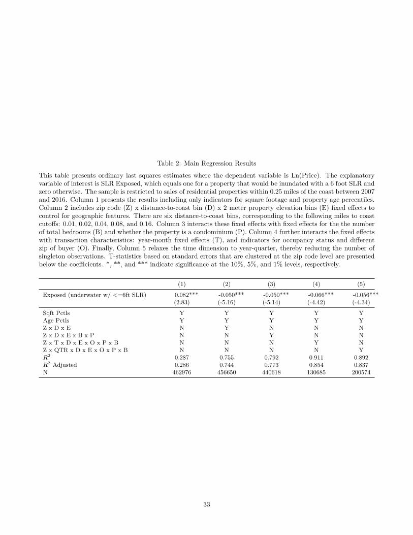
Table 2: Main Regression Results

This table presents ordinary last squares estimates where the dependent variable is Ln(Price). The explanatoryvariable of interest is SLR Exposed, which equals one for a property that would be inundated with a 6 foot SLR andzero otherwise. The sample is restricted to sales of residential properties within 0.25 miles of the coast between 2007and 2016. Column 1 presents the results including only indicators for square footage and property age percentiles.Column 2 includes zip code (Z) x distance-to-coast bin (D) x 2 meter property elevation bins (E) fixed effects tocontrol for geographic features. There are six distance-to-coast bins, corresponding to the following miles to coastcutoffs: 0.01, 0.02, 0.04, 0.08, and 0.16. Column 3 interacts these fixed effects with fixed effects for the the numberof total bedrooms (B) and whether the property is a condominium (P). Column 4 further interacts the fixed effectswith transaction characteristics: year-month fixed effects (T), and indicators for occupancy status and differentzip of buyer (O). Finally, Column 5 relaxes the time dimension to year-quarter, thereby reducing the number ofsingleton observations. T-statistics based on standard errors that are clustered at the zip code level are presentedbelow the coefficients. *, **, and *** indicate significance at the 10%, 5%, and 1% levels, respectively.

(1) (2) (3) (4) (5)

Exposed (underwater w/ <=6ft SLR) 0.082*** -0.050*** -0.050*** -0.066*** -0.056***(2.83) (-5.16) (-5.14) (-4.42) (-4.34)

Sqft Pctls Y Y Y Y YAge Pctls Y Y Y Y YZ x D x E N Y N N NZ x D x E x B x P N N Y N NZ x T x D x E x O x P x B N N N Y NZ x QTR x D x E x O x P x B N N N N YR2 0.287 0.755 0.792 0.911 0.892R2 Adjusted 0.286 0.744 0.773 0.854 0.837N 462976 456650 440618 130685 200574

33

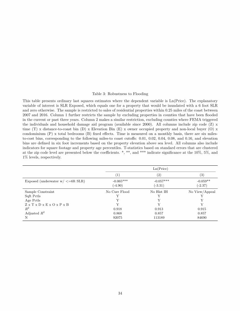
Table 3: Robustness to Flooding

This table presents ordinary last squares estimates where the dependent variable is Ln(Price). The explanatoryvariable of interest is SLR Exposed, which equals one for a property that would be inundated with a 6 foot SLRand zero otherwise. The sample is restricted to sales of residential properties within 0.25 miles of the coast between2007 and 2016. Column 1 further restricts the sample by excluding properties in counties that have been floodedin the current or past three years. Column 2 makes a similar restriction, excluding counties where FEMA triggeredthe individuals and household damage aid program (available since 2000). All columns include zip code (Z) xtime (T) x distance-to-coast bin (D) x Elevation Bin (E) x owner occupied property and non-local buyer (O) xcondominium (P) x total bedrooms (B) fixed effects. Time is measured on a monthly basis, there are six miles-to-cost bins, corresponding to the following miles-to coast cutoffs: 0.01, 0.02, 0.04, 0.08, and 0.16, and elevationbins are defined in six foot increments based on the property elevation above sea level. All columns also includeindicators for square footage and property age percentiles. T-statistics based on standard errors that are clusteredat the zip code level are presented below the coefficients. *, **, and *** indicate significance at the 10%, 5%, and1% levels, respectively.

Ln(Price)

(1) (2) (3)

Exposed (underwater w/ <=6ft SLR) -0.065*** -0.057*** -0.059**(-4.90) (-3.31) (-2.37)

Sample Constraint No Curr Flood No Hist IH No View/AppealSqft Pctls Y Y YAge Pctls Y Y YZ x T x D x E x O x P x B Y Y YR2 0.918 0.913 0.915Adjusted R2 0.868 0.857 0.857N 92075 113189 84690

34

Table 4: Rental Placebo Test

This table presents ordinary least squares estimates where the dependent variable is Ln(Rental Price/Sq. Foot) inColumns 1 and 3, while it is Ln(Rental Price/Sq. Foot) in Columns 2 and 4. The explanatory variable of interest isSLR Exposed, which equals one for a property that would be inundated with a 6 foot SLR and zero otherwise. Thesample is restricted to residential properties within 0.25 miles of the coast and all listings are scraped in Novemberof 2017. Columns 3 and 4 regressions include zip code (Z) x distance-to-coast bin (D) x 2 meter elevation bucket(E) fixed effects. Columns 2 and 4 also include indicators for square footage percentiles. Property ages are notavailable for this sample. We use six distance-to-coast bins, corresponding to the following miles to coast cutoffs:0.01, 0.02, 0.04, 0.08, and 0.16. All columns display T-statistics based on robust standard errors. Columns 2 and4 include percentile buckets for square feet. *, **, and *** indicate significance at the 10%, 5%, and 1% levels,respectively.

ln(price/sqft) ln(price) ln(price/sqft) ln(price)(1) (2) (3) (4)

SLR Exposed 0.034*** 0.046*** -0.003 -0.014(4.61) (6.48) (-0.11) (-1.18)

Sqft Pctls N Y N YZ x D x E x B N N Y YCluster Level Robust Robust Robust RobustR2 0.001 0.350 0.805 0.880Adjusted R2 0.001 0.348 0.759 0.851N 36535 36535 28331 28331

35

Table 5: Exposure and Market Segmentation

This table presents ordinary last squares estimates where the dependent variable is Ln(Price). The explanatoryvariable of interest is SLR Exposed, which equals one for a property that would be inundated with a 6 foot SLRand zero otherwise, along with its interaction with an indicator for a non-owner occupied property (Columns 1and 4), a property sold to a non-local buyer (Columns 2 and 4), and a condominium property (Columns 3 and 4).The sample is restricted to sales of residential properties within 0.25 miles of the coast between 2007 and 2016.All columns include zip code (Z) x time (T) x distance-to-coast bin (D) x Elevation Bin (E) x owner occupiedproperty and non-local buyer (O) x condominium (P) x total bedrooms (B) fixed effects. Time is measured on amonthly basis, there are six miles-to-cost bins, corresponding to the following miles-to coast cutoffs: 0.01, 0.02,0.04, 0.08, and 0.16, and elevation bins are defined in six foot increments based on the property’s elevation abovesea level. All columns also include indicators for square footage and property age percentiles. T-statistics based onstandard errors that are clustered at the zip code level are presented below the coefficients. *, **, and *** indicatesignificance at the 10%, 5%, and 1% levels, respectively.

(1) (2) (3) (4)

Exposed (underwater w/ <=6ft SLR) -0.011 -0.010 -0.033* -0.001(-0.90) (-0.72) (-1.95) (-0.04)

Exposed x Non-Owner Occupied -0.090*** -0.069**(-4.73) (-2.52)

Exposed x Non-Local Buyer -0.079*** -0.027(-4.55) (-1.09)

Exposed x Condo -0.059** -0.009(-2.27) (-0.25)

Sqft Pctls Y Y Y YAge Pctls Y Y Y YZ x T x D x E x O x P x B Y Y Y YR2 0.911 0.911 0.911 0.911Adjusted R2 0.854 0.854 0.854 0.854N 130685 130685 130685 130685

36

Table 6: Exposure Discount In Highly Liquid Market

This table presents ordinary least squares estimates where the dependent variable is either Ln(Price). The ex-planatory variable of interest is SLR Exposed, which equals one for a property that would be inundated with a 6foot SLR and zero otherwise, along with its interaction with measures of liquidity at the zip code level. Liquiditymeasures (Average Sales to List, Inventories, and Days on Market) are normalized by time and county and "HighlyLiquid Market" takes a value of 1 if any liquidity measure is in the most liquid ventile. The sample is restricted tosales of residential properties within 0.25 miles of the coast between 2071 and 2016. In all regressions we includezip code (Z) x time (T) x distance-to-coast bin (D) x Elevation Bin (E) x owner occupied property and non-localbuyer (O) x condominium (P) x total bedrooms (B) fixed effects, and Time is measured on a monthly basis, thereare six miles-to-cost bins, corresponding to the following miles-to coast cutoffs: 0.01, 0.02, 0.04, 0.08, and 0.16, andelevation bins are defined in six foot increments based on the elevation above sea level. All columns also includeindicators for square footage and property age percentiles. T-statistics based on standard errors that are clusteredat the zip code level are presented below the coefficients. *, **, and *** indicate significance at the 10%, 5%, and1% levels, respectively.

(1) (2) (3) (4) (5) (6) (7) (8)

Exposed (underwater w/ <=6ft SLR) -0.107*** -0.035 -0.100*** -0.002 -0.105*** -0.008 -0.106*** 0.003(-5.67) (-0.93) (-5.07) (-0.08) (-5.47) (-0.20) (-5.57) (0.09)

Exposed x Highly Liquid Market 0.069**(2.17)

Exposed x High Sale to List 0.120***(3.45)

Exposed x Low Inventories 0.091***(2.83)

Exposed x Low Days on Market 0.095***(3.52)

OccupancySqft Pctls Y Y Y Y Y Y Y YAge Pctls Y Y Y Y Y Y Y YZ x T x D x E x O x P x B Y Y Y Y Y Y Y YR2 0.890 0.894 0.892 0.925 0.890 0.894 0.890 0.891Adjusted R2 0.822 0.819 0.826 0.855 0.822 0.810 0.823 0.809N 26466 3841 27532 1734 26468 2140 26524 2372

37

Table 7: Beliefs and the Price of Exposure

This table presents ordinary last squares estimates where the dependent variable is Ln(Price). The explanatoryvariable of interest is SLR Exposed, which equals one for a property that would be inundated with a 6 foot SLR andzero otherwise, along with its interaction with Worried, a standardized measure of the level of concern regardingSLR in the county housing the property. Column 3 also interacts SLR Exposed with Worried Mailing FIPS, whichis the same measure as Worried, except that it reflects the worry in county associated with the buyer’s mailingaddress. The sample is restricted to sales of residential properties within 0.25 miles of the coast between 2007and 2016. Column 2 and 3 (4) further restricts the sample to non-owner occupied (owner-occupied) properties.All columns include zip code (Z) x time (T) x distance-to-coast bin (D) x Elevation Bin (E) x owner occupiedproperty and non-local buyer (O) x condominium (P) x total bedrooms (B) fixed effects. Time is measured on amonthly basis, there are six miles-to-cost bins, corresponding to the following miles-to coast cutoffs: 0.01, 0.02,0.04, 0.08, and 0.16, and elevation bins are defined in six foot increments based on the property elevation abovesea level. All columns also include indicators for square footage and property age percentiles. T-statistics based onstandard errors that are clustered at the zip code level are presented below the coefficients. *, **, and *** indicatesignificance at the 10%, 5%, and 1% levels, respectively.

(1) (2) (3) (4)

SLR Exposed -0.077*** -0.098*** -0.102*** -0.025*(-5.43) (-5.16) (-5.17) (-1.82)

Exposed x Worried -0.007 0.017 0.009 -0.044***(-0.36) (0.52) (0.28) (-2.61)

z_worried_2014_buyerfips_exposed 0.003(0.44)

Occupancy All Non-OO Non-OO OOSqft Pctls Y Y Y YAge Pctls Y Y Y YZ x T x D x E x O x P x BR2 0.887 0.883 0.880 0.903Adjusted R2 0.815 0.820 0.817 0.833N 130282 55097 45528 75185

38

Table 8: Price of SLR Over Time

This table presents ordinary last squares estimates where the dependent variable is Ln(Price). The explanatoryvariable of interest is SLR Exposed, which equals one for a property that would be inundated with a 6 foot SLR andzero otherwise, along with its interaction with Time, measured as the natural log of the number of months passedsince the beginning of our sample in January of 2007. The sample is restricted to sales of residential propertieswithin 0.25 miles of the coast between 2007 and 2016. Column 2 (3) further restricts the sample to non-owneroccupied (owner-occupied) properties. All columns include zip code (Z) x time (T) x miles-to-coast bin (D) xelevation bin (E) x owner occupied property and non-local buyer (P) x condominium (C) x total bedrooms (B)fixed effects. Time is measured on a monthly basis, there are six miles-to-cost bins, corresponding to the followingmiles-to coast cutoffs: 0.01, 0.02, 0.04, 0.08, and 0.16, and elevation bins are defined in six foot increments basedon the property elevation above sea level. All columns also include indicators for square footage and property agepercentiles. T-statistics based on standard errors that are clustered at the zip code level are presented below thecoefficients. *, **, and *** indicate significance at the 10%, 5%, and 1% levels, respectively.

(1) (2) (3)

Exposed (underwater w/ <=6ft SLR) 0.029 0.028 0.014(0.87) (0.60) (0.39)

Exposed x Time -0.024*** -0.032*** -0.007(-3.26) (-3.19) (-0.82)

Occupancy All Non-OO OOSqft Pctls Y Y YAge Pctls Y Y YZ x T x D x E x O x P x B Y Y YR2 0.911 0.901 0.924Adjusted R2 0.854 0.846 0.869N 130685 55052 75633

39

Table 9: Prices and Trading Following Information Releases through 2014

This table presents ordinary least squares estimates where the dependent variable is either Ln(Price) or the numberof transactions for a property in a given year (column 4). The explanatory variable of interest is SLR Exposed,which equals one for a property that would be inundated with a 6 foot SLR and zero otherwise, along with itsinteraction with Post-IPCC, which equals one for transactions occurring after 2014 and zero otherwise. The sampleis restricted to sales of residential properties within 0.25 miles of the coast between 2011 and 2016. In all regressionswe include zip code (Z) x time (T) x distance-to-coast bin (D) x Elevation Bin (E) x owner occupied property andnon-local buyer (O) x condominium (P) x total bedrooms (B) fixed effects, and In Columns 2 and 3, restricts thesample to non-owner occupied and owner-occupied properties respectively. Time is measured on a monthly basis,there are six miles-to-cost bins, corresponding to the following miles-to coast cutoffs: 0.01, 0.02, 0.04, 0.08, and0.16, and elevation bins are defined in six foot increments based on the elevation above sea level. All columns alsoinclude indicators for square footage and property age percentiles. T-statistics based on standard errors that areclustered at the zip code level are presented below the coefficients. *, **, and *** indicate significance at the 10%,5%, and 1% levels, respectively.

Log(Price) Volume

(1) (2) (3) (4)

Exposed (underwater w/ <=6ft SLR) -0.068*** -0.087*** -0.019 -0.001(-3.49) (-3.88) (-0.85) (-1.57)

Exposed x Post-2014 -0.021 -0.061** 0.014 0.003**(-0.90) (-2.01) (0.52) (2.01)

Occupancy All Non-OO OO AllSqft Pctls Y Y Y YAge Pctls Y Y Y YZ x T x D x E x O x P x B Y Y Y YR2 0.898 0.885 0.916 0.097Adjusted R2 0.829 0.819 0.851 0.020N 69245 30845 38400 5444952

40

Internet Appendix

A Supplementary Tables and Figures

41

Figure A1: NOAA Sea Level Rise Calculator

Figure A1 displays a sample screenshot from the NOAA Sea Level Rise (SLR) viewer of the New York Metropolitanarea. The viewer provides an online portal to access the underlying SLR shapefiles which describe, for each coastalarea in the Continental USA, detailed data on the properties that will inundated following a 1-6 foot increase inaverage global ocean level. In this case, the light blue regions of the figure represent properties that will becomechronically inundated following a 2 foot increase in global average sea levels.

42

Figure A2: NOAA Exposure Confidence

Figure A2 displays the sea level rise viewer for 6 feet of global average SLR (top) and the confidence level for thesame exposure level (bottom) around Naples FL. Low confidence areas are indicated by orange shading.

43

Figure A3: House Prices vs. Rental Rates (Public vs. Private Data) by Zip Code

Figure A3 demonstrates the quality of the rental listing data scrapped by the authors from Trulia.com. Panel ais a scatter plot of the relationship between median log(rental list price) scrapped for individual properties fromTrulia.com with the log(rental list price) for aggregate data publicly available by zip code from Zillow.com forNovember of 2017. Panel b is a scatter plot of the relationship between median log(rental list price) scrapped onNovember 2017 for individual properties from Trulia.com with the log(median house price) for all property-leveltransactions from the proprietary ZTRAX database from 2007-2016 at the zip code level.

Panel (a)

Panel (b)

44

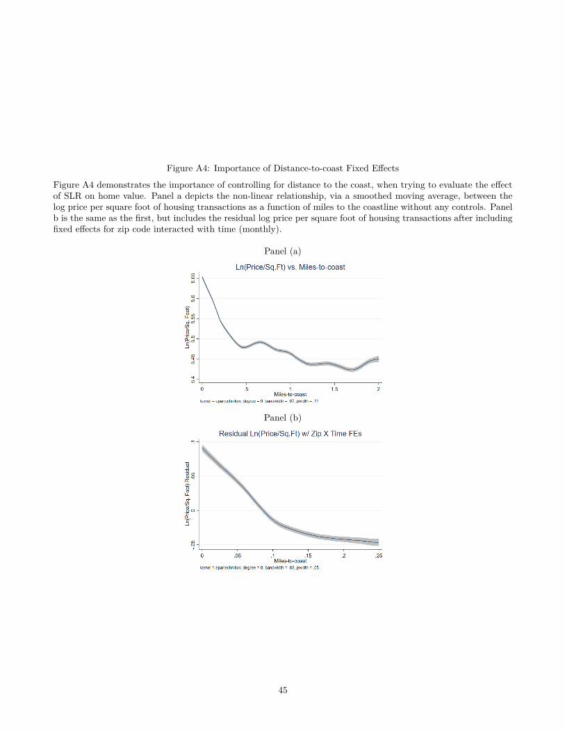
Figure A4: Importance of Distance-to-coast Fixed Effects

Figure A4 demonstrates the importance of controlling for distance to the coast, when trying to evaluate the effectof SLR on home value. Panel a depicts the non-linear relationship, via a smoothed moving average, between thelog price per square foot of housing transactions as a function of miles to the coastline without any controls. Panelb is the same as the first, but includes the residual log price per square foot of housing transactions after includingfixed effects for zip code interacted with time (monthly).

Panel (a)

Panel (b)

45

Figure A5: Google Search Trend for “Sea Level Rise”This Figure displays the Google search intensity for the term sea level rise within the United States from 2004-2017.The vertical axis is normalized by the maximum search activity during the period. The vertical green line indicatesthe release window for parts 2 and 3 of the 2013 IPCC report on climate change.

46

Figure A6: SLR Exposure & House Price Effects over Time - Including "Computed" Prices

Figure A6 replicates Figure 4 demonstrating the relationship between the % change in house price of exposed(relative to unexposed properties) by year for non-owner occupiers for properties within 2 miles of the coast andincluding transactions with RD, CF and CR document types. These coefficients are based on a regression of loghouse price per square foot on categorical dummies for feet of SLR to be exposed after including zip code (Z) x time(T) x distance-to-coast bin (D) x Elevation Bin (E) x non-local buyer (O) x condominium (P) x total bedrooms (B)fixed effects. Time is measured on a monthly basis, there are six miles-to-cost bins, corresponding to the followingmiles-to coast cutoffs: 0.01, 0.02, 0.04, 0.08, and 0.16, and elevation bins are defined in six foot increments basedon the elevation above sea level. The regressions also control for indicators for square footage and property agepercentiles and exclude recently flooded properties. 95% confidence intervals based on standard errors that areclustered by zip code are included as bands in the figure.

47

Table A1: Document Type and Prices

This table describes the three sales price document types within Zillow which account for 99% of transactionsdocumented as full consideration and indicates whether the variable is keyed by Zillow. In addition, it providesthe unexplained variation arising from a regression that includes interacted fixed effects of zip code, month oftransaction, miles to coast buckets, elevation buckets, property and transaction characteristics such as bedrooms,buyer type and view, as well as 20 square foot buckets. Column (4) provides the raw unexplained variation, (5)the adjusted unexplained variation, and (6) the root mean squared error. Finally, (7) provides the non-singletonobservation count.

Sales Code Description Keyed 1−R2 1−R2adj

√MSE N

RD Price obtained from recorded documents Y 2.75% 5.0% 0.18 285,118CF Price computed from transfer tax Y 5.27% 9.81% 0.22 34,619CR Price computed from transfer tax (Rounded) N 5.12% 9.09% 0.23 76,345

48

Table A2: Decomposing Variation in SLR exposure

This table conducts a variance decomposition of abnormal SLR exposure, defined as the residual from regressingSLR exposure on the control variables used in our main analysis (i.e., zip code (Z) x time (T) x distance-to-coast bin(D) x Elevation Bin (E) x owner occupied property and non-local buyer (O) x condominium (P) x total bedrooms(B) fixed effects, and indicators for square footage and property age percentiles. Column 1 presents the R-squaredfrom regressing abnormal exposure on 0.1 meter elevation bins, Column 2 does the same using 0.1 meter elevationbins x zip code fixed effects, and Column 3 further interacts these fixed effects with our seven distance-to-coast binfixed effects.

(1) (2) (3)

0.1M Elevation x Y Y YZip Code x N Y YMiles-to-Coast N N YR2 0.042 0.236 0.344Adjusted R2 0.037 0.116 0.199N 130162 116204 108798

Table A3: Variance Decomposition of SLR Exposure and Price Discount

This table presents ordinary last squares estimates where the dependent variable is Ln(Price). The explanatoryvariables of interest are Explained and Unexplained Residual SLR Exposure. These measures are constructed usingthe residual from a regression of SLR Exposed, an indicator for a property that would be inundated with a 6 footSLR, on indicators for square footage and property age percentiles and zip code (Z) x time (T) x distance-to-coast bin (D) x Elevation Bin (E) x owner occupied property and non-local buyer (O) x condominium (P) x totalbedrooms (B) fixed effects. Time is measured on a monthly basis, there are six miles-to-cost bins, correspondingto the following miles-to coast cutoffs: 0.01, 0.02, 0.04, 0.08, and 0.16, and elevation bins are defined in six footincrements based on the property’s elevation above sea level. Explained Residual SLR Exposure is the portion ofthe residual exposure that is predicted by 0.1 meter x zip code x distance-to-coast bin fixed effects. UnexplainedResidual SLR Exposure is the remainder of the residual SLR exposure. The sample is restricted to sales of residentialproperties within 0.25 miles of the coast between 2007 and 2016. T-statistics based on standard errors that areclustered at the zip code level are presented below the coefficients. *, **, and *** indicate significance at the 10%,5%, and 1% levels, respectively.

(1) (2) (3)

Explained Res. Exposure (0.1 Meter Bin) -0.144*** -0.123***(-4.40) (-3.79)

Unexplained Res. Exposure (0.1 Meter Bin) -0.070*** -0.047***(-4.21) (-2.89)

Sqft Pctls Y Y YAge Pctls Y Y YZ x T x D x E x O x P x B Y Y YR2 0.918 0.918 0.918Adjusted R2 0.868 0.868 0.868N 98483 98483 98483

49

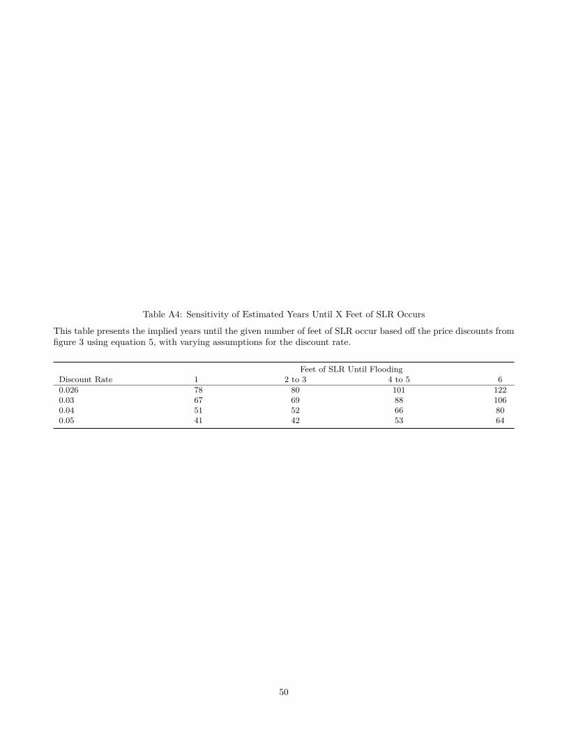
Table A4: Sensitivity of Estimated Years Until X Feet of SLR Occurs

This table presents the implied years until the given number of feet of SLR occur based off the price discounts fromfigure 3 using equation 5, with varying assumptions for the discount rate.

Feet of SLR Until FloodingDiscount Rate 1 2 to 3 4 to 5 60.026 78 80 101 1220.03 67 69 88 1060.04 51 52 66 800.05 41 42 53 64

50

Table A5: Main Results: 2 Miles, Including "Computed" Prices

This table replicates the ordinary last squares estimates from Table 2 including properties within 2 miles of thecoast and including transactions with RD, CF and CR document types. The dependent variable is Ln(Price). Theexplanatory variable of interest is SLR Exposed, which equals one for a property that would be inundated with a 6foot SLR and zero otherwise. The sample is restricted to sales of residential properties within 0.25 miles of the coastbetween 2007 and 2016. Column 1 presents the results including only indicators for square footage and propertyage percentiles. Column 2 includes zip code (Z) x distance-to-coast bin (D) x 2 meter property elevation bins (E)fixed effects to control for geographic features. There are six distance-to-coast bins, corresponding to the followingmiles to coast cutoffs: 0.01, 0.02, 0.04, 0.08, and 0.16. Column 3 interacts these fixed effects with fixed effects forthe the number of total bedrooms (B) and whether the property is a condominium (P). Column 4 further interactsthe fixed effects with transaction characteristics: year-month fixed effects (T), and indicators for occupancy statusand different zip of buyer (O). Finally, Column 5 relaxes the time dimension to year-quarter, thereby reducing thenumber of singleton observations. T-statistics based on standard errors that are clustered at the zip code level arepresented below the coefficients. *, **, and *** indicate significance at the 10%, 5%, and 1% levels, respectively.

(1) (2) (3) (4) (5)

SLR Exposed 0.111*** -0.019** -0.021*** -0.040*** -0.030***(3.89) (-2.50) (-3.06) (-3.06) (-2.84)

Sqft Pctls Y Y Y Y YAge Pctls Y Y Y Y YZ x D x E N Y N N NZ x D x E x B x P N N Y N NZ x T x D x E x O x P x B N N N Y NZ x QTR x D x E x O x P x B N N N N YR2 0.198 0.792 0.826 0.931 0.919R2 Adjusted 0.198 0.784 0.812 0.882 0.872N 3510701 3482051 3396985 826773 1415773

51

Table A6: Additional Results: 2 Miles, Including "Computed" Prices

This table replicates the primary OLS regression specifications from Section 4 including properties within 2 miles ofthe coast and including transactions with RD, CF and CR document types. The dependent variable is Ln(Price).The explanatory variable of interest is SLR Exposed, which equals one for a property that would be inundatedwith a 6 foot SLR and zero otherwise and its interactions with Non-Owner Occupiers (Column 1), "Hot" real estatemarkets (Column 2), County level worriedness about climate change (Column 3) and a log time trend (Column 4).The sample is restricted to sales of residential properties within 2 miles of the coast between 2007 and 2016. Finally,Column 5 relaxes the time dimension to year-quarter, thereby reducing the number of singleton observations. T-statistics based on standard errors that are clustered at the zip code level are presented below the coefficients. *,**, and *** indicate significance at the 10%, 5%, and 1% levels, respectively.

(1) (2) (3) (4)

SLR Exposed 0.004 -0.066*** -0.003 0.006(0.47) (-3.88) (-0.38) (0.28)

Exposed x Non-Owner Occupied -0.080***(-4.42)

Exposed x Highly Liquid Market 0.048*(1.83)

Exposed x Worried -0.019*(-1.76)

Exposed x Time -0.012**(-2.24)

Occupancy All Non-OO OO Non-OOSqft Pctls Y Y Y YAge Pctls Y Y Y YZ x T x D x E x O x P x B Y Y Y YR2 0.931 0.910 0.936 0.931Adjusted R2 0.882 0.849 0.888 0.882N 826773 110214 576355 826773

52

Table A7: View and Amenity Placebos

This table presents evidence that after including the set of fixed effects from our primary specification there is nosignificant relationship between elevation and views. The results are based on ordinary least squares estimates wherethe dependent variable is dummy variable equal to 1 if a property is listed as having "water views". The samplecontains all properties in Column 1, non-owner occupied properties in Column 2, and owner-occupied propertiesin Column 3. The explanatory variable of interest is elevation of the property above sea level in feet. The sampleis restricted to sales of residential properties within 0.25 miles of the coast and includes zip code (Z) x time (T) xdistance-to-coast bin (D) x Elevation Bin (E) x owner occupied property and non-local buyer (O) x condominium(P) x total bedrooms (B) fixed effects. Time is measured on a monthly basis, there are six miles-to-cost bins,corresponding to the following miles-to coast cutoffs: 0.01, 0.02, 0.04, 0.08, and 0.16, and elevation bins are definedin six foot increments based on the elevation above sea level. All columns also include indicators for square footageand property age percentiles. T-statistics based on standard errors that are clustered at the zip code level arepresented below the coefficients. *, **, and *** indicate significance at the 10%, 5%, and 1% levels, respectively.

(1) (2) (3)

Elevation Meters 0.000 0.000 0.000(0.55) (0.07) (0.58)

Occupancy All Non-OO OOSqft Pctls Y Y YDistance to Coast Pctls Y Y YAge Pctls Y Y YZ x T x D x E x O x P x B Y Y YR2 0.832 0.824 0.836Adjusted R2 0.723 0.727 0.717N 130685 58525 75655

53

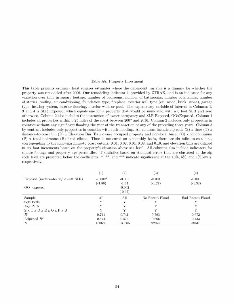
Table A8: Property Investment

This table presents ordinary least squares estimates where the dependent variable is a dummy for whether theproperty was remodeled after 2006. Our remodeling indicator is provided by ZTRAX, and is an indicator for anyvariation over time in square footage, number of bedrooms, number of bathrooms, number of kitchens, numberof stories, roofing, air conditioning, foundation type, fireplace, exterior wall type (ex. wood, brick, stone), garagetype, heating system, interior flooring, interior wall, or pool. The explanatory variable of interest in Columns 1,3 and 4 is SLR Exposed, which equals one for a property that would be inundated with a 6 foot SLR and zerootherwise. Column 2 also includes the interaction of owner occupancy and SLR Exposed, OOxExposed. Column 1includes all properties within 0.25 miles of the coast between 2007 and 2016. Column 2 includes only properties incounties without any significant flooding the year of the transaction or any of the preceding three years. Column 3by contrast includes only properties in counties with such flooding. All columns include zip code (Z) x time (T) xdistance-to-coast bin (D) x Elevation Bin (E) x owner occupied property and non-local buyer (O) x condominium(P) x total bedrooms (B) fixed effects. Time is measured on a monthly basis, there are six miles-to-cost bins,corresponding to the following miles-to coast cutoffs: 0.01, 0.02, 0.04, 0.08, and 0.16, and elevation bins are definedin six foot increments based on the property’s elevation above sea level. All columns also include indicators forsquare footage and property age percentiles. T-statistics based on standard errors that are clustered at the zipcode level are presented below the coefficients. *, **, and *** indicate significance at the 10%, 5%, and 1% levels,respectively.

(1) (2) (3) (4)

Exposed (underwater w/ <=6ft SLR) -0.002* -0.001 -0.001 -0.003(-1.86) (-1.44) (-1.27) (-1.32)

OO_exposed -0.002(-0.65)

Sample All All No Recent Flood Had Recent FloodSqft Pctls Y Y Y YAge Pctls Y Y Y YZ x T x D x E x O x P x B Y Y Y YR2 0.741 0.741 0.793 0.672Adjusted R2 0.574 0.574 0.666 0.433N 130685 130685 92075 38610

54

Table A9: Property Investment, Age, and SLR Discount

This table presents ordinary last squares estimates where the dependent variable is an indicator for a remodeling(Column 1) and Ln(Price) (Columns 2 through 4). Our remodeling indicator is provided by ZTRAX, and is anindicator for any variation over time in square footage, number of bedrooms, number of bathrooms, number ofkitchens, number of stories, roofing, air conditioning, foundation type, fireplace, exterior wall type (ex. wood,brick, stone), garage type, heating system, interior flooring, interior wall, or pool. In Column 1, the explanatoryvariable of interest is an indicator for a transacting property that was built within the past ten years. In Columns2 through 4, the explanatory variable of interest is SLR Exposed, which equals one for a property that would beinundated with a 6 foot SLR and zero otherwise. The sample is restricted to sales of residential properties within0.25 miles of the coast between 2007 and 2016. Columns 2 through 4 include zip code (Z) x time (T) x distance-to-coast bin (D) x Elevation Bin (E) x owner occupied property and non-local buyer (O) x condominium (P) x totalbedrooms (B) fixed effects. Time is measured on a monthly basis, there are six miles-to-cost bins, correspondingto the following miles-to coast cutoffs: 0.01, 0.02, 0.04, 0.08, and 0.16, and elevation bins are defined in six footincrements based on the propertys elevation above sea level. All columns also include indicators for square footageand property age percentiles. Column(s) 2 (3 and 4) restricts the sample to properties that were built in the last10 (5) years. Column 4 also excludes recently flooded properties. T-statistics based on standard errors that areclustered at the zip code level are presented below the coefficients. *, **, and *** indicate significance at the 10%,5%, and 1% levels, respectively.

Remodel Rate Ln(Price)

(1) (2) (3) (4)

Property Age <= 10 Years -0.063***(-4.25)

Exposed (underwater w/ <=6ft SLR) -0.095*** -0.062** -0.053*(-3.14) (-2.23) (-1.91)

Age All < 10 Years < 5 Years < 5 YearsIncludes Flooded Y Y Y NSqft Pctls Y Y Y YAge Pctls N Y Y YZ x T x D x E x O x P x B Y Y Y YR2 0.861 0.949 0.951 0.948Adjusted R2 0.772 0.918 0.924 0.920N 138451 23877 16139 13655

55

Table A10: Age and Square Footage Placebos

This table presents ordinary least squares estimates where the dependent variable is the natural log of one plusproperty age and property square footage in Columns 1 and 2, respectively. The explanatory variable of interest isSLR Exposed, which equals one for a property that would be inundated with a 6 foot SLR and zero otherwise. Thesample is restricted to sales of residential properties within 0.25 miles of the coast. In all regressions we include zipcode (Z) x time (T) x distance-to-coast bin (D) x Elevation Bin (E) fixed effects. Time is measured on a monthlybasis, there are six miles-to-cost bins, corresponding to the following miles-to coast cutoffs: 0.01, 0.02, 0.04, 0.08,and 0.16, and elevation bins are defined in six foot increments based on the elevation above sea level. T-statisticsbased on standard errors that are clustered at the zip code level are presented below the coefficients. *, **, and*** indicate significance at the 10%, 5%, and 1% levels, respectively.

Ln(Age) Ln(Sqft)

(1) (2)

Exposed (underwater w/ <=6ft SLR) 0.005 0.017(0.18) (1.18)

Z x T x D x E Y YR2 0.687 0.656Adjusted R2 0.526 0.482N 254889 263738

Table A11: Buyer Education and Income

This table presents ordinary last squares estimates where the dependent variable captures either education orincome levels at the buyer’s zip code. In column (1) the dependent variable is percentage of bachelor attainment,column (2) is the natural log of income, column (3) is the percentage bachelor attainment at the buyer zip minusthat at the property zip and column (4) is the log ratio of incomes between buyer and property zip. T-statisticsbased on standard errors that are clustered at the zip code level are presented below the coefficients. *, **, and*** indicate significance at the 10%, 5%, and 1% levels, respectively.

(1) (2) (3) (4)

Owner Occupied -0.034*** -0.054***(-5.86) (-3.35)

Constant 0.418*** 11.161*** 0.040*** 0.145***(74.48) (713.70) (7.60) (7.73)

R2 0.008 0.005 0.000 0.000Adjusted R2 0.008 0.005 0.000 0.000N 433204 432223 194578 193491

56

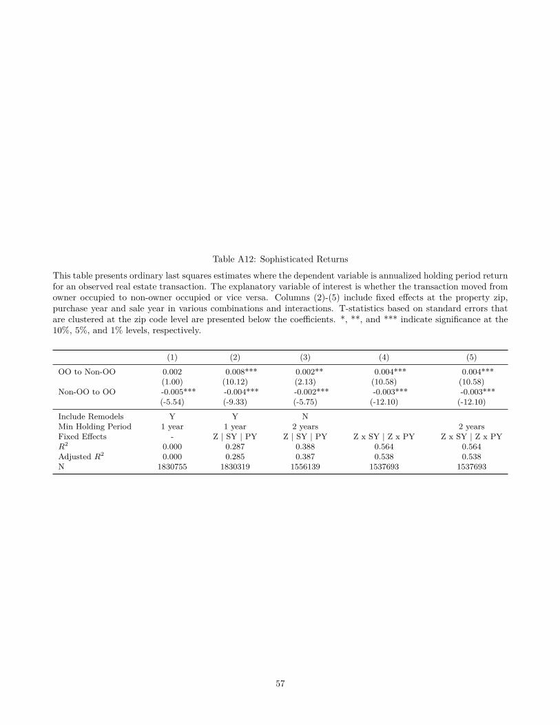
Table A12: Sophisticated Returns

This table presents ordinary last squares estimates where the dependent variable is annualized holding period returnfor an observed real estate transaction. The explanatory variable of interest is whether the transaction moved fromowner occupied to non-owner occupied or vice versa. Columns (2)-(5) include fixed effects at the property zip,purchase year and sale year in various combinations and interactions. T-statistics based on standard errors thatare clustered at the zip code level are presented below the coefficients. *, **, and *** indicate significance at the10%, 5%, and 1% levels, respectively.

(1) (2) (3) (4) (5)

OO to Non-OO 0.002 0.008*** 0.002** 0.004*** 0.004***(1.00) (10.12) (2.13) (10.58) (10.58)

Non-OO to OO -0.005*** -0.004*** -0.002*** -0.003*** -0.003***(-5.54) (-9.33) (-5.75) (-12.10) (-12.10)

Include Remodels Y Y NMin Holding Period 1 year 1 year 2 years 2 yearsFixed Effects - Z | SY | PY Z | SY | PY Z x SY | Z x PY Z x SY | Z x PYR2 0.000 0.287 0.388 0.564 0.564Adjusted R2 0.000 0.285 0.387 0.538 0.538N 1830755 1830319 1556139 1537693 1537693

57

Table A13: Buyer Type and SLR Discount

This table presents ordinary least squares estimates where the dependent variable is either Ln(Price). The explana-tory variable of interest is SLR Exposed, which equals one for a property that would be inundated with a 6 footSLR and zero otherwise, along with its interaction with the type of purchaser. The sample is restricted to salesof residential properties within 0.25 miles of the coast and only includes non-owner occupiers. In all regressionswe include zip code (Z) x time (T) x distance-to-coast bin (D) x Elevation Bin (E) x owner occupied propertyand non-local buyer (O) x condominium (P) x total bedrooms (B) fixed effects, and In Panel a Column 2 (3) andPanel b column 3 (4) restricts the sample to non-owner occupied (owner-occupied) properties. Time is measuredon a monthly basis, there are six miles-to-cost bins, corresponding to the following miles-to coast cutoffs: 0.01,0.02, 0.04, 0.08, and 0.16, and elevation bins are defined in six foot increments based on the elevation above sealevel. All columns also include indicators for square footage and property age percentiles. T-statistics based onstandard errors that are clustered at the zip code level are presented below the coefficients. *, **, and *** indicatesignificance at the 10%, 5%, and 1% levels, respectively.

(1) (2) (3)

Exposed (underwater w/ <=6ft SLR) -0.104*** -0.094*** -0.097***(-5.02) (-4.79) (-5.33)

Second Home Waiver 0.072***(7.77)

Exposed x Second Home -0.009(-0.69)

Company Buyer 0.081***(2.97)

Exposed x Company Buyer 0.000(0.00)

Occupancy Second Home Non-OO Non-OOSqft Pctls Y Y YAge Pctls Y Y YZ x T x D x E x O x P x B Y Y YR2 0.889 0.901 0.901Adjusted R2 0.811 0.847 0.846N 6873 55052 55052

58

Table A14: Market Segmentation

This table presents the transistion probability matrix between owner occupied properties and non-owner occupiedproperties.

Occupancy Before TransactionOccupancy After Transaction Non-OO OO Total

% % %Non-OO 78.7 15.3 42.4OO 21.3 84.7 57.6Total 100.0 100.0 100.0

59

B Buyer Sophistication

Evidence in Robinson (2012) indicates that individuals purchasing properties that they will not occupy tend to

have better credit scores and higher incomes than owner-occupied buyers, consistent with those households being

more likely to engage in sophisticated transactions. In this Appendix, we provide two types of empirical evidence

consistent with the non-owner occupiers in our sample being more sophisticated buyers. First, we utilize the zip

code of the purchaser to link our transactions database with the education and income data from the American

Community Survey from Census. Table A11 provides a simple univariate analysis of the education and income

differentials between owner occupiers and non-owner occupiers. Column (1) displays the results of a regression

with the percentage of bachelor achievement at the buyer’s mailing address on the left hand side and a dummy

variable that takes a value of 1 if the purchaser is an owner occupier on the right hand side. Here, we see that owner

occupiers are likely to have mailing addresses associated with 4% less bachelor degree attainment than non-owner

occupiers. A similar gap exists in income as seen in column (2) where owner occupiers as associated with areas

that have 11% lower income than non-owner occupiers. In addition, we compare the education and income levels

of non-owner occupiers with those at the zip of the property in columns (3) and (4). We see similar magnitude

differentials between education and income, suggesting that non-owner occupying buyers appear to come from areas

that are more educated and have higher income per capita than the properties they purchase.

To augment the evidence on buyer sophistication, we examine annualized holding period returns as an ex-post

measure of investor performance. For all coastal counties we find any properties with repeat transactions utilizing

the same screening criteria as described in section 2.1. We then cross-reference transactions with the historical tax

records provided in ZTRAX to identify the occupancy status prior to and after purchase. Our hypothesis is that, if

non-owner occupiers are more sophisticated then they will benefit at the expense of owner occupiers. In particular,

transactions where an owner occupier purchases a house from a non-owner occupier should be associated with lower

holding period returns, and transactions where a non-owner occupier purchases from an owner occupier should have

higher holding period returns. Table A12 displays the results from a regression following the specification in equation

7 below.

AnnRetit = β1OOtoNOOit + β2NOOtoOOit + λz,ty,py + εit (7)

Column (1) provides a bivarate analysis with no control variables for all properties held for longer than one year.

A positive β1 and a negative and significant β2 are consistent with the hypothesis of non-owner occupying buyers

being more sophisticated. To tighten our analysis, we include zip, purchase year and sale year fixed effects. Here,

both β1 and β2 are indicate that non-owner occupiers earning higher returns. Flippers—investors that purchase

a property, quickly improve it, then sell it–may play a role in our finding, particularly in biasingβ1 upward. In

column (3) we extend the minimum holding period to 2 years, and eliminate any transactions where a remodeling

60

has occurred. Consistent with flippers playing a role in the positive returns accruing in OO to Non-OO transactions,

the magnitude of β1 drops from 80bps per year to around 20bps, while β2 cuts in half. Finally, in columns (4)

and (5) we include zip interacted with year of purchase and zip interacted with year of sale fixed effects, and the

triple interaction of zip, year of purchase and year of sale fixed effects, respectively. Across models (3)-(5) the

coefficients remain relatively stable, declining in magnitude only slightly as we absorb more variation with fixed

effects. Column (5) implies that the higher returns are not coming from location or timing of purchase, but perhaps

the opportunistic buying and selling of properties, consistent with a sophisticated investor.

61

C Sample Selection and Robustness�

As discussed in Section 2.1, we focus our tests on properties within 1/4 mile of the nearest coast or shoreline. This

sample restriction is chosen to balance the trade-off between including the maximum number of communities and

properties that are exposed to SLR with the fact that the confidence in the NOAA’s exposure measure decreases with

the distance from the coast. Within the quarter mile band, approximately 30% of properties are SLR exposed. By

contrast, only 5% of transactions 0.25 to 1.0 miles from the coast are of exposed properties and this figure drops to

2% using a 1.0 to 2.0 mile bandwidth. Thus, our sample contains the vast majority of communities with substantial

SLR exposure. Figure A2 provides an example of how the NOAA’s exposure measure becomes less certain further

from the coast. The low confidence areas (orange) begin as close as a quarter mile from the shoreline and are

common within a mile. Unfortunately, NOAA does not provide the confidence level as an easily usable shapefile,

so we are unable to interact our analysis with the confidence levels.

In addition, we restrict our sample to transactions where prices are recorded directly from the sales documents

(“RD” transactions.) Two additional types of transactions appear frequently in the Zillow transactions database,

“CF” and “CR”, corresponding to “Full Consideration - Computed from Transfer Tax” and “Computed from Trans-

fer Tax; county rounds sales price prior to tax computation when necessary” respectively. Table A1 substantiates

our original decision to focus on only RD documents. We run a “kitchen sink” approach to explaining the transac-

tion prices of properties within 2 miles of the coast. In particular, we interact zip code, month of transaction, miles

to coast buckets extended at 0.08 mile increments to the 2 mile bound, elevation buckets, property and transaction

characteristics, as well as 20 square foot buckets. As shown in the Residual Variation column, only 2.75% of the

variation remains unexplained in the RD sample, while over 5% remains unexplained for transactions where the

sales price is not directly coded. Adjusted residual variation and root mean squared errors tell a similar story,

prices are significantly less noisy in the RD document type than other price codes19.

While we believe this sample provides the cleanest estimates of SLR risk, our results are not dependent on

these choices. We replicate the main insights of this paper including all transactions within 2 miles of the coast

and adding the “CF” and “CR” document types and in Figure A6, and Tables A5 and A6 below. We find that the

estimated SLR exposure discount changes slightly in magnitude but not in interpretation or statistical significance.

In particular, our average coefficient for the main specification moves from -0.066 to -0.040. While we find that the

error bounds on the year-by-year sample have increased slightly, Figure A6 illustrates the same general trend as in

the previous sample. In addition, our results are still significant when excluding flooded properties or those views.

Finally, in our rental placebo tests (not shown) our fully specified coefficients are indistinguishable from zero.19These findings are qualitatively consistent with reports by Zillow on their website. They give only one star for their confidence

(out of 4 possible stars) for properties in areas where “Tax assessor’s value” rather than prices directly from documents are available.See www.zillow.com/zestimate for more details.

62

We assess the robustness of our cross sectional results from section 4 in Table A6. First, as shown in Column

(1), the non-OO interaction coefficient remains nearly identical. In column (2), we combine our liquidity indicators

and show that when we focus on any hot market, the effect of exposure attenuates significantly for non-OO buyers.

In Column (3) we show that within the OO segment, worried counties price SLR risk. Finally in Column (4) we

corroborate the figure by showing that the coefficient has been diminishing over time.

63