Discovering Hotspots: A Placement Strategy forWi-Fi based Trajectory Monitoring within Buildings

Lorenz SchauerMobile and Distributed Systems Group

Ludwig-Maximilians UniversitatMunich, Germany

Email: lorenz.schauer@ifi.lmu.de

Abstract—In the last decade, Wi-Fi based trajectory monitor-ing has gathered high interest in the scientific and commercialworld, due to the increased usage of Wi-Fi capable mobile devices.A lot of work can be found where monitor nodes are placed inan area of interest capturing Wi-Fi signals from passing phones.However, the deployment of such nodes is often inefficient,expressed by a low ratio between monitored trajectories andthe amount of installed nodes. Hence, finding an optimal settingof node positions is an essential and challenging task. In thispaper, a systematic solution for this variant of the NP-hardart gallery problem is investigated. The idea is to set monitornodes only on places (hotspots), where most of the human pathscan be tracked. For the discovery of such hotspots, three novelapproaches are presented working on simulated user traces basedon an extended pathway mobility model, and a given plant layout.The results of each approach are evaluated in terms of qualityfor Wi-Fi based trajectory monitoring using different parametersand settings. The evaluation indicates that the proposed methodsshow different potentials and limitations. Overall, they return areliable setting of hotspots compared to a completely randomselection of an equal amount of node positions and, thus, theyserve as a systematic and sophisticated placement strategy.

Keywords—Hotspot Discovery; Node Placement; Art gallery;Mobility Model; Trajectory Clustering

I. INTRODUCTION

The immense diffusion of modern mobile devices withintegrated sensors and several communication interfaces haveled to an increased usage of Wi-Fi as de facto wirelesscommunication standard. In many situations and locations ofdaily life, e.g. at work, at home, in shopping malls or in otherpublic places, wireless networks are available, offering Internetaccess and local services to people. In order to use theseservices in an ubiquitous way, Wi-Fi enabled mobile devicesperiodically scan their vicinity for known or free networksand try to connect to them automatically. Such 802.11 activescans leak unencrypted information to the surroundings, e.gthe device-specific MAC-address, and can easily be capturedby any Wi-Fi card set into monitor mode. A lot of work inliterature can be found where an infrastructure of several Wi-Fi monitor nodes has been deployed into an area of interestto gather crowd data [4], social relationships [3], or estimatepedestrian flows [16], and track human trajectories [15].

However, the deployment strategy of such nodes is neverfurther explained. E.g., the authors in [4] express that 15monitor nodes “were placed at strategic locations”, but it is

not discussed if the same or more mobile devices could havebeen tracked with a smaller amount of nodes placed at otherlocations. In other words, the ratio between the amount oftracked devices and the number of used monitor nodes is notinvestigated in terms of efficiency, and a random selectionof node positions does not return the best solution. Adequatesetup strategies and approaches for finding optimal positionswithin a given scenario are still missing. Due to the fact, thateach additional monitor node leads to higher installation andmaintenance cost and causes more overhead in communicationand data analysis, such approaches would help to save moneyby reducing the amount of required nodes without decreasingthe amount of trackable devices.

In this paper, we focus on this optimization problemfor a Wi-Fi based trajectory monitoring infrastructure withinlarge public buildings. Such an infrastructure captures Wi-Fi signals from passing phones at various places in orderto reproduce the original trajectories, represented as a seriesof coordinates, taken by the visitors of the building. Forthis purpose, we simulate various visitors moving througha bitmap representation of a floor plan on an underlyingextended pathway mobility model. Based on these simulations,we try to find the best locations for the placement of monitornodes in a given building. In order to reach this goal, wepresent and implement three approaches returning potentialnode positions: A grid-based method, a density clusteringmethod using DBSCAN [8], and a trajectory clustering methodusing the TRACLUS [14] algorithm. The positions returned bythese methods are evaluated in terms of quality for Wi-Fi basedtrajectory monitoring and are compared against a completelyrandom selection of the same amount of nodes.

The goal is, that a maximum amount of human trajectoriescan be tracked by a minimum amount of monitor nodes.Intuitively, the best location for a monitor node is foundwhen it’s range covers those areas which are frequented bya maximum amount of people. In a heatmap, these areaswould be represented as “very hot” and, hence, the best andoptimal positions for Wi-Fi monitors are called “hotspots” inthis context. The contributions of this paper can be summarizedas follows:

• A variant of the well-known art gallery problem ispresented

• An extension of the pathway mobility model [2] is in-troduced in order to simulate visitors inside buildings

• Three novel approaches for finding the most fre-DOI: 10.1109/IntelliSys.2015.7361169 $33.00 c©2015 IEEE

quented areas are presented and evaluated on differentenvironments and for various input parameters

• An alternative method for the partitioning phase of theTRACLUS algorithm is presented, resulting in a moreprecise segmentation phase for human trajectorieswithin buildings and reducing the computational effortfor clustering, due to less segmentation points.

The paper is organized as follows: Section II gives abrief overview of related work. Some preliminaries and theproblem statement are presented in Section III. Based onthese definitions, the methodology is described in SectionIV introducing the used models and three hotspot discoveryapproaches. The evaluation of these approaches is presentedin Section V and, finally, Section VI concludes the paper andgives hints on future work.

II. RELATED WORK

This paper is related to current research topics, suchas hotspot discovery, Wi-Fi based trajectory estimation, andstrategies for sensor placement. Thiagarajan et al. [17] analyzecollected data from Wi-Fi captures and estimate both humantrajectories and travel times in street networks. Road segmentswith lots of traffic are named as hotspots which are discoveredwhen a remarkable high travel time is observed. Hoteit etal. [11] also use the term of hotspots for the most crowdedregions in cellular networks. Based on data from mobilephone activities, the authors estimate human trajectories usingdifferent interpolation methods and discover hotspots with amedian error lower than 7%. Ahmed et al. [1] define hotspotsas a location with a user density higher than a predefinedthreshold. Based on this definition, an approach is presentedreturning all of the existing hotspots based on indoor trackingdata. In comparison to these works, we define hotspots as thecenter of regions which are passed by a maximum amountof people. This is similar to the hot route discovery problem,trying to find the most frequently traveled routes [6], [19].

Several real word experiments can be found deploying acertain amount of Wi-Fi monitor nodes in an area of interestin order to estimate human trajectories [9], [15]. However,adequate placement strategies are not discussed further andapproaches for finding the best node locations are still missing.In general, finding optimal locations for sensor nodes is a bigchallenge and a lot of research is done in this field. Differentstrategies and techniques for node placement in wireless sensornetworks are presented in literature [18]. An optimization isintroduced by Krause et al. [12], [13], trying to find the k bestlocations for sensor nodes in an area of interest where a finiteset of possible node locations exists. An optimized solutionfor visual sensor placement is presented by Gonzalez [10], orBottino and Laurentini [5]. Both works present an algorithmin order to solve a variation of the art gallery problem whichis similar to the problem statement of this paper. However, ourapproach focuses on discovering hotspots for efficient Wi-Fibased trajectory monitoring within buildings, and to the bestof our knowledge, this has not been investigated so far.

III. DEFINITIONS AND PROBLEM STATEMENT

The overall goal is to monitor a maximum amount ofhuman trajectories with a minimum amount of deployed nodes.

Obviously, this goal has two opposed properties: The mini-mization of deployed nodes and the maximization of trackablehuman paths. In order to reach this goal, the following defini-tions are introduced before presenting the problem statement:

A trajectory t is a time-series of location records repre-senting a human path Pi. In our context, Pi is representedas a sequence of two-dimensional points p, denoted as Pi ={p1, p2, ..., pn}. Inside a building, a person moves withinwalkable regions along a spatial network of floors, rooms,halls, etc.

According to [14], each trajectory t can be partitionedat characteristic points, where the behavior of t changessignificantly. We only consider the direction of a person’smovement for choosing characteristic points, due to the factthat a person usually walks straight along shortest paths andsuddenly changes the walk direction on certain locations, e.g.corners, doors, entries, etc, rather than walking completelyrandom. Hence, a characteristic point is defined as followsin this context:

Definition 1 (Characteristic Point): A point p ∈ Pi ismarked as characteristic point cp ∈ Pi when the directionvector νt changes at p with an angle α ≥ 4.

On the basis of such characteristic points, we define sub-trajectories:

Definition 2 (Sub-trajectory): A sub-trajectory τ ⊆ t rep-resents a partition of a trajectory t and is denoted as a linesegment between two successive characteristic points cpncpmwith n < m.

In order to monitor a complete trajectory as accurate aspossible, it becomes necessary to be able to track a maximumamount of its sub-trajectories:

Definition 3 (Trackable Sub-trajectory): A sub-trajectoryτ is trackable, if there is at least one point p ∈ τ locatedwithin the coverage range rm of at least one monitor node m,formally desired as:

∃p ∈ τ.∃m ∈M : dist(p,m) ≤ rm (1)

where dist(p,m) is the Euclidean distance between the mon-itor node m and one point p of the sub-trajectory τ .

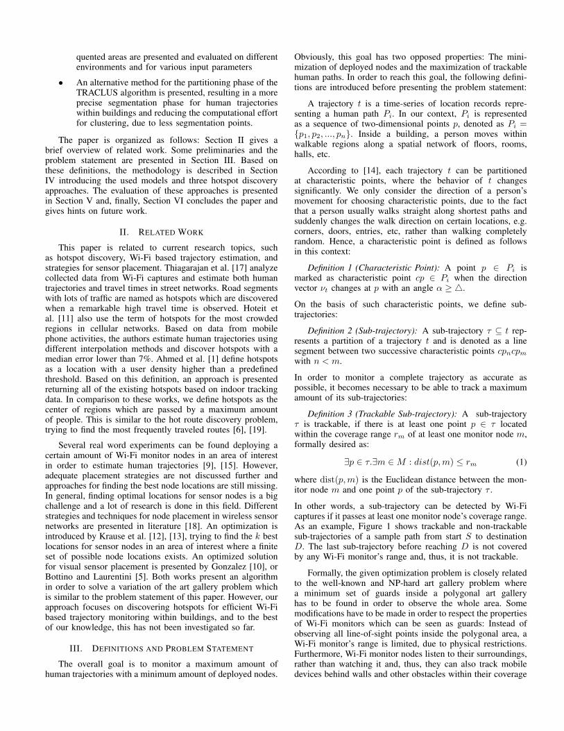
In other words, a sub-trajectory can be detected by Wi-Ficaptures if it passes at least one monitor node’s coverage range.As an example, Figure 1 shows trackable and non-trackablesub-trajectories of a sample path from start S to destinationD. The last sub-trajectory before reaching D is not coveredby any Wi-Fi monitor’s range and, thus, it is not trackable.

Formally, the given optimization problem is closely relatedto the well-known and NP-hard art gallery problem wherea minimum set of guards inside a polygonal art galleryhas to be found in order to observe the whole area. Somemodifications have to be made in order to respect the propertiesof Wi-Fi monitors which can be seen as guards: Instead ofobserving all line-of-sight points inside the polygonal area, aWi-Fi monitor’s range is limited, due to physical restrictions.Furthermore, Wi-Fi monitor nodes listen to their surroundings,rather than watching it and, thus, they can also track mobiledevices behind walls and other obstacles within their coverage

DS

Characteristic Points

Trackable Sub-Trajectory

Non-Trackable Sub-Trajectory

Monitor Node

Range

Fig. 1. Example of trackable and non-trackable sub-trajectories

range. According to [10], and with respect to the proposedmodifications, the problem statement is defined as follows:

Definition 4 (Problem Statement): Given a polygonal lay-out Γ ⊂ R2 and a set of human trajectories T . Find a minimumset of monitor node (guard) locations G = {gm1 , gm2 , ..., gmn}with coverage range rm1 , rm2 , ..., rmn inside of Γ, such thata maximum set of sub-trajectories τ is trackable from at leastone point in G according to Definition 3.

In order to solve this problem, monitor nodes should be de-ployed at locations where most people pass by, and thus, wherethe most sub-trajectories are trackable. As already mentioned,these locations are called “hotspots”. The following sectionintroduces a methodology with three different approaches foran automatic detection of such hotspots.

IV. METHODOLOGY

The algorithms presented in this section are based onhuman trajectories created by simulated persons moving insidebuildings. For the building’s representation, a simple, andmetrical environment model is used.

A. Environment Model

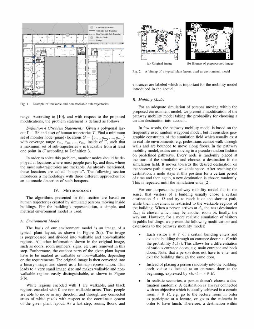
The basis of our environment model is an image of atypical plant layout, as shown in Figure 2(a). The imageis preprocessed and divided into walkable and non-walkableregions. All other information shown in the original image,such as doors, room numbers, signs, etc., are removed in thisstep. Furthermore, the outdoor parts of the given plant layouthave to be marked as walkable or non-walkable, dependingon the requirements. The original image is then converted intoa binary image, and stored as a bitmap representation. Thisleads to a very small image size and makes walkable and non-walkable regions easily distinguishable, as shown in Figure2(b).

White regions encoded with 1 are walkable, and blackregions encoded with 0 are non-walkable areas. Thus, peopleare able to move in any direction and through any connectedareas of white pixels with respect to the coordinate systemof the given plant layout. As a last step, rooms, floors, and

(a) Original image (b) Bitmap of preprocessed image

Fig. 2. A bitmap of a typical plant layout used as environment model

entrances are labeled which is important for the mobility modelintroduced in the sequel.

B. Mobility Model

For an adequate simulation of persons moving within theproposed environment model, we present a modification of thepathway mobility model taking the probability for choosing acertain destination into account.

In few words, the pathway mobility model is based on thefrequently used random waypoint model, but it considers geo-graphic constraints of the simulation field which usually existin real life environments, e.g. pedestrians cannot walk throughwalls and are bounded to move along floors. In the pathwaymobility model, nodes are moving in a pseudo-random fashionon predefined pathways. Every node is randomly placed atthe start of the simulation and chooses a destination in thesimulation field. It moves towards the desired destination onthe shortest path along the walkable space. After reaching thedestination, a node stays at this position for a certain periodof time and then again, a new destination is chosen randomly.This is repeated until the simulation ends [2].

For our purpose, the pathway mobility model fits in thesense, that visitors of a building usually chose a certaindestination d ∈ D and try to reach it on the shortest path,while their movement is restricted to the walkable regions ofthe building. When a person arrives at di, the next destinationdi+1 is chosen which may be another room or, finally, theway out. However, for a more realistic simulation of visitorsin public buildings, we present the following modifications andextensions to the pathway mobility model:

• Each visitor v ∈ V of a certain building enters andexits the building through an entrance door e ∈ E withthe probability Pv(e). This allows for a differentiationof various entrance doors, e.g. main entrance and backdoors. Note, that a person does not have to enter andexit the building through the same door.

• Instead of placing a person randomly into the building,each visitor is located at an entrance door at thebeginning, expressed by start = e ∈ E.

• In realistic scenarios, a person doesn’t choose a des-tination randomly. A destination is always connectedwith an objective which is usually achieved in a certainroom r ∈ R, e.g. go to the lecture room in orderto participate at a lecture, or go to the cafeteria inorder to have lunch. Therefore, a destination within

Require: environment modelV:= number of Visitorsfor (v = 1 : V ) doD := number of Destinations/*choose entrance e with probability Pv(e)*/start = getEntranceDoor()for (d = 1 : D) do

if (d == D) then/*choose exit e with probability Pv(e)*/d = getEntranceDoor();

else/*choose destination d with probability Pv(d)*/d = get next Destination();

end if/*compute shortest path between start and d*/path = compute dijkstra(start, d);/*Store path for visitor v*/savePathPerV isitor(path, v);start = d;

end forend for

Fig. 3. Simulation algorithm of the proposed mobility model

a building is usually a room, rather than a floor orstaircase. Thus, in our mobility model a destination isdefined as d→ roomx.

• Only the last destination dlast of a visitor must be anexit door in order to leave the building: dlast → e,and e is chosen with the probability Pv(e).

• Any destination is chosen by a visitor at a certain timet with the probability Pv,t(d). This modulation allowsfor a more realistic simulation of choosing destinationswith respect to the time, a decision is made. E.g.,a lecture room is visited more before lessons, andthe cafeteria is visited more during lunch time. Somerooms are chosen with a higher probability than othersat the same time, e.g, the main lecture room comparedto smaller ones.

The simulation algorithm for the proposed mobility modelis depicted in Figure 3. In summary, we create a certainamount of visitors V and let them move on shortest pathsfrom start to the particular destination through a given building.Each visitor chooses a number of destinations w.r.t the givenprobabilities and leaves the building through an entrance dooras last destination.

C. Hotspot Discovery Approaches

As already mentioned, hotspots in this context represent aset of locations inside a given building where Wi-Fi monitornodes should be placed in order to track human trajectoriesin an efficient way. On the basis of the proposed simulations,three approaches are introduced in the sequel, allowing for asystematic discovery of such hotspots.

1) Grid-Based: As a first step, the grid-based approachcreates a heatmap representation of the simulated trajectories.Such a heatmap illustrates how often a certain location inthe building has been visited. Every time a person passes a

pixel coordinate of the bitmap, the corresponding heat value isincreased by one. For a better illustration, Figure 4 representssuch a heatmap of 1000 simulated persons each choosing fivedestinations in a main building of a big university.

Fig. 4. Heatmap of 1000x5 simulated paths in a university building.

In the second step, a square grid with constant square widthws is placed over the heatmap, and the pixel sum of eachsquare sΣ is stored together with the pixel coordinates of thecorresponding square center cs. This results in a list L →<cs, sΣ > indicating the frequency of how often a square hasbeen visited by a person. The list entries cs and sΣ dependon ws. In our case, this parameter is set as ws = mr ·

√2

and, hence, a monitor node’s coverage radius mr serves asthe minimum bounding circle of a square. Thus, every pixelcoordinate inside the building can be observed, when monitornodes are only allowed to be placed at the square centers ofthe grid.

As a last step, hotspots are determined out of all squarecenters cs ∈ L. Formally, a square center cs is marked ashotspot if sΣ ≥ ε·arg maxsΣ∈L{sΣ}, with 0 ≤ ε ≤ 1. In otherwords, if the pixel sum of a square is greater than a certainpercentage ε of the most frequented square, the location ofits center is marked as hotspot. Obviously, the result dependsdirectly on ε which has to be chosen individually, accordingto the given requirements.

Note, this simple approach only considers how often asquare is frequented by visitors, rather than respecting thecourse of trajectories. Thus, essential points of human paths,e.g. where significant direction changes occur, may not becovered by any node if the pixel sum of the particular squareis low and, hence, important information for tracking humanmovements is getting lost. In order to solve this problem, wepresent the following approach focusing on direction changesof human trajectories.

2) Density-Based: This approach is called density-based,because it uses the DBSCAN algorithm [8] in order to performa density based clustering of characteristic points. Centers ofdiscovered clusters are then marked as hotspots. The algorithmof this approach is shown in Figure 5.

Require: A set of trajectories T = {t1, t2, ..., ti}Parameters: ε, minPts, and ε

/*Step 1: Find characteristic points/*for all (ti ∈ T ) doindex = 1;Add p1 ∈ ti to the set CPi of characteristic points;len = 1;v1 = createV ector(pindex, pindex+len);while ((index+ 2 · len) ≤ length(ti)) dov2 = createV ector(pindex+len, pindex+2·len);if (vectorAngle(v1, v2) ≥ 1

3π) thenAdd pindex+len to CPi;v1 = v2;

end ifindex++;

end whileAdd last point of ti to CPi;/*Use Douglas-Peucker to smooth CPi*/SPi = performDouglasPeucker(CPi, ε);Add SPi to result set R;

end for

/*Step 2: Get clusters of characteristic points*/Cl = DBSCAN(R,minPts, ε);return mean(cli ∈ Cl); /*Cluster centers*/

Fig. 5. Algorithm of density-based approach for hotspot discovery

As a first step, the characteristic points are determinedand extracted from the simulated trajectories. According toDefinition 1, a characteristic point is found when the directionvector changes with α ≥ 4. As shown in Figure 5, we set4 = 1

3π. Thus, points are marked as characteristic, if thewalk direction changes with at least 60◦. Intuitively, this is areasonable value for indoor scenarios where persons usuallychange their walk direction rapidly with α ≈ 90◦, e.g. whenturning around a corner, or entering a room.

In our simulations, however, we also observe particulardirection changes of the trajectory with α ≈ 90◦ when aperson walks next to an obstacle or a wall. This is caused bycomputing shortest paths on bitmaps where each white pixelrepresents a possible location, and a simulated path can runalong a wall pixel per pixel, as it is shown in Figure 6. Dueto this fact, many characteristic points are extracted by ouralgorithm which do not represent a real direction change of aperson, depicted as little circles in Figure 6(a). Hence, thesepoints should not be marked as characteristic and have to beremoved from the set of CPi. For this purpose, we use the linesimplification algorithm of Douglas-Peucker [7], and smootheach trajectory of characteristic points CPi with a small εvalue. As an example, the results of this step are shown inFigure 6(b) using ε = 7. The remaining characteristic pointsSPi of each trajectory are added to the result set R.

In the second step, R is given as input parameter to theDBSCAN algorithm in order find density based clusters ofcharacteristic points. Note that results of DBSCAN dependsignificantly on the required input parameters minPts and εdetermining the minimal number of points required to forma dense region within an ε neighborhood radius. In our case,

(a) Before smoothing

(b) After using Douglas-Peucker

Fig. 6. Extracted characteristic points on simulated paths

this radius is set w.r.t. a monitor node’s coverage range asupper bound: ε ≤ rm. Furthermore, we restrict minPts with1 ≤ minPts ≤ |T |, so a cluster has to contain less or equalpoints than the amount of given trajectories. A higher value forminPts leads to very big clusters which are not practicable forour purpose. The parameter minPts allows to react on distinctsituations or individual requirements for node placement: ifminPts = 1, the most clusters are detected, and lead to amaximum amount of hotspots, and also to a higher probabilityfor tracking all visitors. For minPts = |T | less clusters (downto one single cluster) are found leading to a minimum amountof discovered hotspots, but also to a minimum number oftrackable trajectories.

Finally, the center of each cluster is computed as themean of all cluster points. The set of all center pointsC = {Ccl1 , Ccl2 , ..., Cclm} is returned and represents the setof discovered hotspots.

Considering the time complexity, the proposed algorithmshows a linear complexity O(n) for the discovery of charac-teristic points, where n is the number of points on a trajectoryti. The complexity of Douglas-Peucker is O(n2) in worstcase, with n = |CPi| denoting the number of discoveredcharacteristic points of a trajectory ti. The complexity ofDBSCAN is also O(n), with n = |R| in this case.

In comparison to the grid-based method, this approachconsiders the course of trajectories focusing on rapid direc-tion changes. In the following section, an extension to thismethod is presented, considering more characteristics of sub-trajectories for a reliable tracking of human paths.

3) Trajectory-Based: The trajectory-based approach usesthe TRACLUS algorithm [14] in order to find representativetrajectories of clusters. Such clusters are formed through adensity-connected set of similar sub-trajectories. Due to theusage of Dijkstra for shortest path routing, we only considercharacteristic points according to Definition 1 for the partition-ing of trajectories. Hence, we use the presented algorithm forfinding characteristic points from the previous section, ratherthan computing the MDL cost for each point of a line segment,as described in [14]. The proposed modification is suitablefor our purpose resulting in a more precise and less complexpartitioning phase for human trajectories within buildings.

Furthermore, less segmentation points are returned reducingthe computational effort of TRACLUS’ grouping phase.

This phase performs a density-based clustering of linesegments using principles of DBSCAN. Again, two parametersminLns and ε are required in order to build clusters of linesegments. A cluster is then formed by a density connected setaround core line segments which have a minimum amountof lines minLns within their ε-neighborhood. Like before,we define ε ≤ rm and 1 ≤ minLns ≤ |T |, so we focuson clusters containing a minimum amount of minLns sub-trajectories within a monitor’s coverage range. This is veryuseful for our purpose, where monitor nodes should only beplaced in areas where many people pass by.

As a last step, the TRACLUS algorithm introduces amethod for constructing representative trajectories RT . For thediscovery of hotspots, we highly benefit from this step, becauseeach representative trajectory rti ∈ RT represents the charac-teristic movement of all sub-trajectories of the correspondingcluster cli. Important parts of human paths are described bythe representative trajectories and, hence, they are required tobe trackable according to Definition 3. A basic solution wouldbe to install one monitor node m for each rti ∈ RT such thatEquation 1 is satisfied. However, this solution would requiretoo many nodes, because some representative trajectories mightbe close together and could be covered by one single node.Hence, we use DBSCAN with ε = rm and minPts = 1 inorder to group start and endpoints of representative trajectorieswhich are located in a range of one monitor node. The centersof returned clusters are marked as hotspots. Note that noisypoints of this step are not removed. They are rather consideredas hotspots, because these points represent particular start orendpoints which are not in the vicinity to others and cannotbe clustered by DBSCAN.

V. EVALUATION

In this section, the presented approaches are evaluated indifferent environments and for a various amount of simulatedpaths. First of all, we investigate the effect of required inputparameters, e.g. ε, minPts, or minLns for each approach. Af-terwards, the returned hotspots are evaluated against a randomselection of monitor node positions with respect to the amountof trackable sub-trajectories.

A. Settings

Four plant layouts are used for evaluation, representingdifferent characteristics and probabilities for choosing a certaindestination:

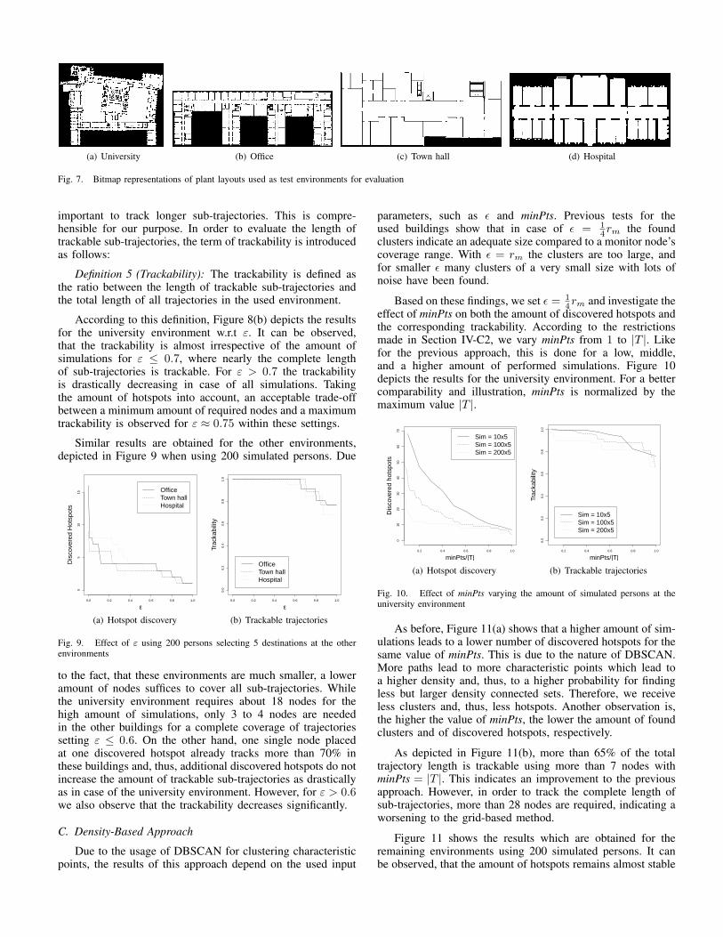
1) The principle building of a university, where lecturehalls are selected with a higher probability accordingto their capacity, and entrances are used on the basisof their importance, e.g. the main entrance is usedwith a higher probability than side entrances. Thecorresponding plant layout is depicted in Figure 7(a)representing the biggest environment of our evalua-tion.

2) An office environment, where offices are visited withthe same probability and special rooms, e.g. confer-ence room, cafeteria, toilette, etc., can be visited more

often depending on the scenario. The environment isillustrated in Figure 7(b).

3) A town hall, where a lot of people are attended eachday. Thus, the probability of choosing the waitingand public office is much higher than going to themayor’s office. Figure 7(c) depicts the town hall.

4) A hospital floor, with one operating room and severaldorms. Again, the main entrance is chosen with ahigher probability than both side entrances and thedorms are selected according to the number of beds.The hospital is illustrated in Figure 7(d).

On each of these environments, we perform 20 simulationscreating a small amount of 10 up to a higher amount of200 persons choosing 5 destinations inside the correspondingbuilding. As a simplification, and, due to the fact that wehave no adequate Wi-Fi propagation model for each of theenvironments, the coverage range of a monitor node is set torm = 25 meter which is a realistic value for indoor scenarios.

B. Grid-Based Approach

As described in Section IV-C1, a square center is markedas hotspot, if the pixel sum of the square is greater or equalthan a certain factor ε of the most frequented square. Forevaluation, we vary ε from 0.00 to 1.00 for each environment.Furthermore, we investigate the influence of the simulationsand create 10, 100, and 200 persons selecting 5 destinationswithin each building. The results for the university building asthe largest environment are depicted in Figure 8(a). Obviously,

0.0 0.2 0.4 0.6 0.8 1.0

010

2030

4050

Dis

cove

red

hots

pots

ε

Sim = 10x5Sim = 100x5Sim = 200x5

(a) Hotspot discovery

0.0 0.2 0.4 0.6 0.8 1.0

0.0

0.2

0.4

0.6

0.8

1.0

ε

Trac

kabi

lity

Sim = 10x5Sim = 100x5Sim = 200x5

(b) Trackable trajectories

Fig. 8. Effect of ε varying the amount of simulated persons at the universityenvironment

the amount of square centers which are marked as hotspotsincreases with decreasing ε. For ε = 1.0, one hotspot isreturned denoting the most frequented square. On the opposite,for ε = 0.0 every square center is marked as hotspot. Itis shown, that in case of less simulations, more squares aremarked as hotspots for the same ε value, particularly forε > 0.5. This is evident, because the pixel sums of squaresare not as different as in case of more simulations and, hence,more square centers are marked as hotspots when decreasingε.

As next step, we evaluate how many sub-trajectories aretrackable according to Definition 3 when placing monitornodes at the discovered hotspots. More precisely, we considerthe length of these trackable sub-trajectories, rather than justtheir amount. The length can be seen as a weight for eachtrackable sub-trajectory, leading to the fact, that it is more

(a) University (b) Office (c) Town hall (d) Hospital

Fig. 7. Bitmap representations of plant layouts used as test environments for evaluation

important to track longer sub-trajectories. This is compre-hensible for our purpose. In order to evaluate the length oftrackable sub-trajectories, the term of trackability is introducedas follows:

Definition 5 (Trackability): The trackability is defined asthe ratio between the length of trackable sub-trajectories andthe total length of all trajectories in the used environment.

According to this definition, Figure 8(b) depicts the resultsfor the university environment w.r.t ε. It can be observed,that the trackability is almost irrespective of the amount ofsimulations for ε ≤ 0.7, where nearly the complete lengthof sub-trajectories is trackable. For ε > 0.7 the trackabilityis drastically decreasing in case of all simulations. Takingthe amount of hotspots into account, an acceptable trade-offbetween a minimum amount of required nodes and a maximumtrackability is observed for ε ≈ 0.75 within these settings.

Similar results are obtained for the other environments,depicted in Figure 9 when using 200 simulated persons. Due

0.0 0.2 0.4 0.6 0.8 1.0

05

1015

Dis

cove

red

Hot

spot

s

ε

OfficeTown hallHospital

(a) Hotspot discovery

0.0 0.2 0.4 0.6 0.8 1.0

0.0

0.2

0.4

0.6

0.8

1.0

Trac

kabi

lity

ε

OfficeTown hallHospital

(b) Trackable trajectories

Fig. 9. Effect of ε using 200 persons selecting 5 destinations at the otherenvironments

to the fact, that these environments are much smaller, a loweramount of nodes suffices to cover all sub-trajectories. Whilethe university environment requires about 18 nodes for thehigh amount of simulations, only 3 to 4 nodes are neededin the other buildings for a complete coverage of trajectoriessetting ε ≤ 0.6. On the other hand, one single node placedat one discovered hotspot already tracks more than 70% inthese buildings and, thus, additional discovered hotspots do notincrease the amount of trackable sub-trajectories as drasticallyas in case of the university environment. However, for ε > 0.6we also observe that the trackability decreases significantly.

C. Density-Based Approach

Due to the usage of DBSCAN for clustering characteristicpoints, the results of this approach depend on the used input

parameters, such as ε and minPts. Previous tests for theused buildings show that in case of ε = 1

4rm the foundclusters indicate an adequate size compared to a monitor node’scoverage range. With ε = rm the clusters are too large, andfor smaller ε many clusters of a very small size with lots ofnoise have been found.

Based on these findings, we set ε = 14rm and investigate the

effect of minPts on both the amount of discovered hotspots andthe corresponding trackability. According to the restrictionsmade in Section IV-C2, we vary minPts from 1 to |T |. Likefor the previous approach, this is done for a low, middle,and a higher amount of performed simulations. Figure 10depicts the results for the university environment. For a bettercomparability and illustration, minPts is normalized by themaximum value |T |.

0.2 0.4 0.6 0.8 1.0

010

2030

4050

6070

Dis

cove

red

hots

pots

minPts/|T|

Sim = 10x5Sim = 100x5Sim = 200x5

(a) Hotspot discovery

0.2 0.4 0.6 0.8 1.0

0.0

0.2

0.4

0.6

0.8

1.0

minPts/|T|

Trac

kabi

lity

Sim = 10x5Sim = 100x5Sim = 200x5

(b) Trackable trajectories

Fig. 10. Effect of minPts varying the amount of simulated persons at theuniversity environment

As before, Figure 11(a) shows that a higher amount of sim-ulations leads to a lower number of discovered hotspots for thesame value of minPts. This is due to the nature of DBSCAN.More paths lead to more characteristic points which lead toa higher density and, thus, to a higher probability for findingless but larger density connected sets. Therefore, we receiveless clusters and, thus, less hotspots. Another observation is,the higher the value of minPts, the lower the amount of foundclusters and of discovered hotspots, respectively.

As depicted in Figure 11(b), more than 65% of the totaltrajectory length is trackable using more than 7 nodes withminPts = |T |. This indicates an improvement to the previousapproach. However, in order to track the complete length ofsub-trajectories, more than 28 nodes are required, indicating aworsening to the grid-based method.

Figure 11 shows the results which are obtained for theremaining environments using 200 simulated persons. It canbe observed, that the amount of hotspots remains almost stable

0.0 0.2 0.4 0.6 0.8 1.0

010

2030

4050

Dis

cove

red

Hot

spot

s

minPts/|T|

OfficeTown hallHospital

(a) Hotspot discovery

0.0 0.2 0.4 0.6 0.8 1.0

0.0

0.2

0.4

0.6

0.8

1.0

Trac

kabi

lity

minPts/|T|

OfficeTown hallHospital

(b) Trackable trajectories

Fig. 11. Effect of minPts using 200 persons selecting 5 destinations at theother environments

for minPts > 0.6|T |, indicating that distinct clusters are foundwithin these environments. In case of the town hall, the twodiscovered hotspots for minPts = |T | suffice for a nearlycomplete tracking of all trajectories which is a good result.In case of the hospital more than 75% can be tracked usingat least two nodes, and 94% with 5 nodes. However, for theoffice environment, the discovered hotspots show an overallimpractical trackability, where only 84% of the total length ofsub-trajectories can be tracked using 2 nodes.

D. Trajectory-Based Approach

Node placement based on representative trajectories is avery promising method, due to focusing on trajectories whichalready represent the most significant pedestrian flows. How-ever, the clustering results of TRACLUS are critical referredto the required parameters ε and minLns. The ε-neighborhoodof a line segment is forming an ellipsoid, rather than a circleas in case of DBSCAN when using points. Hence, we cannotset ε = 1

4rm like in the previous approach and have to evaluatethe quality of discovered hotspots according to our constraintsmade in Section IV-C3. Again, we vary both parameters with1 ≤ ε ≤ rm and 1 ≤ minLns ≤ |T | and investigateboth, the amount of discovered hotspots and the correspondingtrackability for different simulations and environments. Ourinvestigations indicate, that for ε ≈ 1

8rm, and minLns ≤ 10adequate clusters are found. For minLns > 10 more and moreline segments are declared as noise and important clustersare destroyed. The effect of minLns for 10, 100, and 200simulated persons choosing 5 destinations at the universitybuilding with ε = 1

8rm is shown in Figure 12. In contrastto the previous approaches, the amount of simulations highlyinfluence the results w.r.t minLns, as depicted in Figure12(a).In case of 10x5 simulations, a maximum amount of 20 hotspotsis discovered with minLns = 3 leading to a nearly completecoverage of all sub-trajectories. For minLns > 3 the amount ofdiscovered hotspots decreases, due to an increased number ofline segments which are marked as noise leading to destroyedclusters. In contrast, more simulations augment the density oftrajectories and, hence, less but bigger clusters are found fora small value of minLns. When increasing minLns, more butsmaller clusters are discovered leading to more representativetrajectories. The higher the amount of simulations, the higherthe density of start and endpoints of representative trajectoriesand the more can be grouped by DBSCAN and represented byone single hotspot, as observed for both dashed lines in Figure

0 2 4 6 8 10

05

1015

2025

30

Dis

cove

red

hots

pots

minLns

Sim = 10x5Sim = 100x5Sim = 200x5

(a) Hotspot discovery

0 2 4 6 8 10

0.0

0.2

0.4

0.6

0.8

1.0

minLns

Trac

kabi

lity

Sim = 10x5Sim = 100x5Sim = 200x5

(b) Trackable trajectories

Fig. 12. Effect of minLns varying the amount of simulated persons at theuniversity environment

12. The best result (optimal trade-off between a minimumamount of required nodes and a maximum trackability) for100x5 simulations is obtained with minLns = 4 tracking97.9% of the complete length of trajectories using 17 nodes.In case of 200x5 simulations, 15 hotspots are discovered withminLns = 6 tracking 98.3% in best case.

Again, the results for the other environments using 200x5simulations with ε = 1

8rm are depicted in Figure 13. Like be-fore, the amount of discovered hotspots increases with highervalues for minLns, as depicted in Figure 13(a). Obviously,the effect of minLns is not as high as in case of a hugeenvironment, due to a higher density of trajectories in smallbuildings. Only 3, 3, and 2 hotspots suffice to track 99.8%(minLns = 2), 99.3% (minLns = 6), and 94.4% (minLns = 6)at the office, town hall, and hospital, respectively. Again, theseresults announce the best trade-off between a minimum amountof required nodes and a maximum trackability.

0 2 4 6 8 10

02

46

810

Dis

cove

red

hots

pots

minLns

OfficeTown hallHospital

(a) Hotspot discovery

0 2 4 6 8 10

0.0

0.2

0.4

0.6

0.8

1.0

minLns

Trac

kabi

lity

OfficeTown hallHospital

(b) Trackable trajectories

Fig. 13. Effect of minLns using 200 persons selecting 5 destinations at theother environments

E. Tracking Quality

The goal is to evaluate the quality of efficient Wi-Fi basedmonitoring with respect to the trackability when using thediscovered hotspots. For this purpose, we use the most naivemethod and select randomly the same amount of nodes as weget by the performed approach on the used environment. Thenode positions are selected from the complete set of possiblepositions which are all white pixels of the used plant layoutin our case. Note, that the optimal node placement is alsoincluded in this set of possible positions. In order to reachalways the optimal solution, every possible k-node permutation

of all n possible positions have to be checked according tothe trackability which requires

(nk

)operations. This is too

complex in case of huge bitmaps, though. Therefore, we use anapproximate solution. We repeat the selection of node positions100,000 times and take the best result with respect to itstrackability. Beside the fact, that the selection is still random,we assume that this method approximates the optimal solutionof node placement, due to the high amount of repetitions. Thus,we take the result as a quality measure for the discoveredhotspots when using optimal input parameters.

Table I depicts the results for each environment usingthe proposed approach with the denoted parameters on 200x5simulated paths. In order to evaluate and compare the qualityof discovered hotspots, the last two rows show the trackabilityusing the stated amount of nodes at the discovered hotspots,or at the best randomly selected positions. Considering thetrackability, it is shown that there is only a marginal differ-ence of up to 0.137 between the best random selection ofpositions and the discovered hotspots for each approach, andfor all environments. This indicates that the proposed methodsreturn a reliable setting of node positions for an efficientWi-Fi based monitoring system. However, the density-basedapproach never returns a setting of hotspots showing a higheror equal trackability than the corresponding random selection.Therefore, we conclude that clustering of points representingonly the direction changes of human paths is not an optimalplacement strategy w.r.t the proposed quality measure, becauseit never reaches the optimal solution within the given settings.This is caused by the fact, that other characteristics, e.g. thetrajectories’ length, are not considered by this approach and,hence, longer trajectories may not be covered by any nodeleading to a decreased trackability.

We overcome this problem using the trajectory-based ap-proach which considers the complete course of importantsub-trajectories. With this method, we obtain the best resultscompared to our quality measure. Besides from the town hall,the trajectory-based approach always reaches a higher tracka-bility than the corresponding best random selection and, thus,node placement based on representative trajectories indicatesa sophisticated and quite optimal solution. According to theseresults, Figure 14 illustrates the 15 discovered hotspots as littlecircles within the university building. It is shown, that thedepicted hotspots apparently mark strategic places inside thebuilding, due to the fact, that each entrance door and everyedge of principle hallways are observed by at least on node.This indicates a reasonable setting for Wi-Fi monitor nodes.However, the required parameters, such as minLns, and ε of theTRACLUS algorithm highly influence these results and, thus,they have to be selected carefully w.r.t to the given settings asit is shown in the previous section.

In contrast, the grid-based approach requires only onecertain threshold ε which allows to find an optimal trade-off between a minimum amount of nodes and a maximaltrackability. As depicted in Table I, adequate results havebeen found for 0.7 ≤ ε ≤ 0.83. Compared to the bestrandom selection, the grid-based approach performed betterin the hospital, equal in the town hall, but worse in the office,and the university building. However, it still shows betterresults than the density-based approach and requires less inputparameters. Therefore, this simple approach can be seen as

Fig. 14. Little circles denote the hotspots in the university building discoveredby the trajectory-based approach.

a first systematic method to find good places for monitornodes, but it cannot replace a more advanced solution likethe trajectory-based approach.

VI. CONCLUSION AND FUTURE WORK

In this paper, we have addressed the need for an adequateplacement strategy of monitor nodes inside buildings for anefficient Wi-Fi based trajectory monitoring system. In order tofind the best places for monitor nodes, which can be seen asa variant of the well-studied and NP-hard art gallery problem,three novel approaches for discovering hotspots have been pre-sented. The proposed methods all work on bitmaps of typicalplant layouts and simulated trajectories generated according toa modified pathway mobility model. While the first approachonly considers local information from a heatmap, the last twoperform density-based clustering on different characteristics oftrajectories.

The evaluation of the proposed approaches on differentenvironments and settings leads to the conclusion, that the pre-sented methods allow for a systematic discovery of adequatenode positions compared to a completely random selection ofnodes. However, the density-based approach using DBSCANon characteristic points never reaches a trackability higherthan the proposed quality measure. In contrast, the grid-basedapproach is very simple, shows better results, and requires lessinput parameters. It can be seen as an easy and systematicmethod to find quite adequate node positions, but it does notalways return the best solution for the tested environmentsw.r.t our quality measure. As a more sophisticated solution,the trajectory-based approach performs best and returns a quiteoptimal solution for most environments. However, it is morecomplex and requires more input parameters which have to bedetermined carefully, due to their high influence on the results.

In summary, we conclude that the presented approachescan reliably support the decision process for an adequate nodeplacement of monitor nodes within a certain building. The eval-uation has shown, that even our most simple approach leadsto a better trackability using less monitors than an arbitrary

Environment University Office Town Hall HospitalApproach Grid Density Trajectory Grid Density Trajectory Grid Density Trajectory Grid Density Trajectory

Parameters ε=0.73 ε 14 rm ε = 1

8 rm ε=0.83 ε = 14 rm ε = 1

8 rm ε=0.73 ε = 14 rm ε = 1

8 rm ε=0.70 ε = 14 rm ε = 1

8 rmminPts=25 minLns=6 minPts=25 minLns=2 minPts=200 minLns=3 minPts=30 minLns=6

# Hotspots 13 15 15 4 2 3 3 2 3 3 5 2Trackability(Approach) 0.929 0.912 0.982 0.997 0.842 0.999 1.000 0.997 0.991 0.952 0.941 0.944

Trackability(Random) 0.979 0.981 0.981 1.000 0.979 0.998 1.000 0.999 1.000 0.947 0.991 0.928

TABLE I. AMOUNT OF NODES WITH REACHED TRACKABILITY USING HOTSPOTS COMPARED TO THE BEST RANDOM SELECTION OF NODE POSITIONS

installation of nodes, as often performed in related work. Inprinciple, the findings of this paper are not only usable for Wi-Fi monitor nodes. The proposed approaches are also adoptablefor any kind of wireless node placement, such as Bluetoothbeacons or other sensor nodes. However, we focus on Wi-Fi,because we plan to realize a real world deployment of Wi-Fimonitor nodes for pedestrian flow monitoring on the basis ofthe discovered hotspots for future work. Furthermore, we planto find a suitable heuristic to determine the optimal parametersfor the clustering approaches in a given environment, andwe want to enhance our evaluation focusing on other qualitymeasures within bigger indoor environments.

REFERENCES

[1] T. Ahmed, T. B. Pedersen, and H. Lu. Capturing hotspots forconstrained indoor movement. In Proceedings of the 21st InternationalConference on Advances in Geographic Information Systems, SIGSPA-TIAL’13, pages 472–475. ACM, 2013.

[2] F. Bai and A. Helmy. A survey of mobility models. Wireless AdhocNetworks. University of Southern California, USA, 206, 2004.

[3] M. V. Barbera, A. Epasto, A. Mei, V. C. Perta, and J. Stefa. Signalsfrom the crowd: uncovering social relationships through smartphoneprobes. In Proceedings of the 2013 conference on Internet measurementconference, pages 265–276. ACM, 2013.

[4] B. Bonne, A. Barzan, P. Quax, and W. Lamotte. Wifipi: Involuntarytracking of visitors at mass events. In World of Wireless, Mobileand Multimedia Networks (WoWMoM), 2013 IEEE 14th InternationalSymposium and Workshops on a, pages 1–6. IEEE, 2013.

[5] A. Bottino and A. Laurentini. A nearly optimal algorithm for coveringthe interior of an art gallery. Pattern recognition, 44(5):1048–1056,2011.

[6] Z. Chen, H. T. Shen, and X. Zhou. Discovering popular routes fromtrajectories. In Data Engineering (ICDE), 2011 IEEE 27th InternationalConference on, pages 900–911. IEEE, 2011.

[7] D. H. Douglas and T. K. Peucker. Algorithms for the reduction of thenumber of points required to represent a digitized line or its caricature.Cartographica: The International Journal for Geographic Informationand Geovisualization, 10(2):112–122, 1973.

[8] M. Ester, H.-P. Kriegel, J. Sander, and X. Xu. A density-based algorithmfor discovering clusters in large spatial databases with noise. In Kdd,volume 96, pages 226–231, 1996.

[9] Y. Fukuzaki, M. Mochizuki, K. Murao, and N. Nishio. A pedestrianflow analysis system using wi-fi packet sensors to a real environment.In Proceedings of the International Joint Conference on Pervasive andUbiquitous Computing: Adjunct Publication, UbiComp ’14 Adjunct,pages 721–730. ACM, 2014.

[10] H. Gonzalez-Banos. A randomized art-gallery algorithm for sensorplacement. In Proceedings of the seventeenth annual symposium onComputational geometry, pages 232–240. ACM, 2001.

[11] S. Hoteit, S. Secci, S. Sobolevsky, C. Ratti, and G. Pujolle. Estimatinghuman trajectories and hotspots through mobile phone data. ComputerNetworks, 64:296–307, 2014.

[12] A. Krause, R. Rajagopal, A. Gupta, and C. Guestrin. Simultaneousoptimization of sensor placements and balanced schedules. AutomaticControl, IEEE Transactions on, pages 2390–2405, 2011.

[13] A. Krause, A. Singh, and C. Guestrin. Near-optimal sensor placementsin gaussian processes: Theory, efficient algorithms and empirical stud-ies. The Journal of Machine Learning Research, pages 235–284, 2008.

[14] J.-G. Lee, J. Han, and K.-Y. Whang. Trajectory clustering: a partition-and-group framework. In Proceedings of the 2007 ACM SIGMODinternational conference on Management of data, pages 593–604. ACM,2007.

[15] A. Musa and J. Eriksson. Tracking unmodified smartphones using wi-fimonitors. In Proceedings of the 10th ACM Conference on EmbeddedNetwork Sensor Systems, pages 281–294. ACM, 2012.

[16] L. Schauer, M. Werner, and P. Marcus. Estimating crowd densitiesand pedestrian flows using wi-fi and bluetooth. In Proceedings of11th International Conference on Mobile and Ubiquitous Systems:Computing, Networking and Services. EAI, 2014.

[17] A. Thiagarajan, L. Ravindranath, K. LaCurts, S. Madden, H. Balakr-ishnan, S. Toledo, and J. Eriksson. Vtrack: Accurate, energy-awareroad traffic delay estimation using mobile phones. In Conference onEmbedded Networked Sensor Systems, SenSys ’09, pages 85–98. ACM,2009.

[18] M. Younis and K. Akkaya. Strategies and techniques for node placementin wireless sensor networks: A survey. Ad Hoc Networks, 6(4):621–655,2008.

[19] K. Zheng, Y. Zheng, X. Xie, and X. Zhou. Reducing uncertaintyof low-sampling-rate trajectories. In Data Engineering (ICDE), 28thInternational Conference on, pages 1144–1155. IEEE, 2012.