DI

SC

US

SI

ON

P

AP

ER

S

ER

IE

S

Forschungsinstitut zur Zukunft der ArbeitInstitute for the Study of Labor

How Fast Do Wages Adjust to Human-CapitalProductivity? Dynamic Panel-Data Evidencefrom Belgium, Denmark and Finland

IZA DP No. 4583

November 2009

Corrado Andini

How Fast Do Wages Adjust to Human-Capital Productivity?

Dynamic Panel-Data Evidence from Belgium, Denmark and Finland

Corrado Andini Universidade da Madeira,

CEEAplA and IZA

Discussion Paper No. 4583 November 2009

IZA

P.O. Box 7240 53072 Bonn

Germany

Phone: +49-228-3894-0 Fax: +49-228-3894-180

E-mail: iza@iza.org

Any opinions expressed here are those of the author(s) and not those of IZA. Research published in this series may include views on policy, but the institute itself takes no institutional policy positions. The Institute for the Study of Labor (IZA) in Bonn is a local and virtual international research center and a place of communication between science, politics and business. IZA is an independent nonprofit organization supported by Deutsche Post Foundation. The center is associated with the University of Bonn and offers a stimulating research environment through its international network, workshops and conferences, data service, project support, research visits and doctoral program. IZA engages in (i) original and internationally competitive research in all fields of labor economics, (ii) development of policy concepts, and (iii) dissemination of research results and concepts to the interested public. IZA Discussion Papers often represent preliminary work and are circulated to encourage discussion. Citation of such a paper should account for its provisional character. A revised version may be available directly from the author.

IZA Discussion Paper No. 4583 November 2009

ABSTRACT

How Fast Do Wages Adjust to Human-Capital Productivity? Dynamic Panel-Data Evidence from Belgium, Denmark and Finland* The standard human-capital model is based on the assumption that the observed wage of an individual is equal to the monetary value of the individual net human-capital productivity, the so-called net potential wage. We argue that this assumption is rejected by the ECHP data for Belgium, Denmark and Finland. The empirical evidence supports a dynamic approach to the Mincer equation where no equality is imposed but an adjustment between observed and potential earnings is allowed to take place over time. Controlling for regressors’ endogeneity, individual heterogeneity and time effects, we estimate a dynamic panel-data wage equation and provide measures of the speed of adjustment in Belgium, Denmark and Finland. Further, we elaborate on the implications of a dynamic approach to the Mincer equation for the computation of the return to schooling, including the implication that this return is not independent of labor-market experience, as suggested by Heckman et al. (2005) and Belzil (2007). Finally, we show that a dynamic wage equation can be seen as the solution of a simple wage-bargaining model and argue that a micro-founded model can fit the data better than a simple adjustment model but requires more theoretical assumptions. JEL Classification: I21, J31 Keywords: Mincer equation, wages, human capital Corresponding author: Corrado Andini Universidade da Madeira Campus da Penteada 9000-390 Funchal Portugal E-mail: andini@uma.pt

* Financial support from the European Commission (EDWIN project, HPSE-CT-2002-00108) is gratefully acknowledged. The usual disclaimer applies.

1

1. Introduction In the standard human-capital model proposed by Mincer (1974), the logarithm of the hourly observed earnings of an individual is explained by schooling years, potential labor-market experience and experience squared. This section presents the theoretical foundations of the standard Mincerian equation as reported by Heckman et al. (2003). Therefore, we make no claim of originality at this stage and mainly aim at helping the reader with notations and terminology adopted in the next sections. Mincer argues that potential earnings today depend on investments in human capital made yesterday. Denoting potential earnings at time t as tE , Mincer assumes that an individual invests in human capital a share tk of his potential earnings with a return of

tr in each period t. Therefore we have: (1) )kr1(EE ttt1t +=+ which, after repeated substitution, becomes:

(2) ∏−

=

+=1t

0j0jjt E)kr1(E

or alternatively:

(3) ∑−

=

++=1t

0jjj0t )kr1ln(ElnEln .

Under the assumptions that:

• schooling is the number of years s spent in full-time investment ( 1k...k 1s0 === − ),

• the return to schooling in terms of potential earnings is constant over time

( β=== −1s0 r...r ),

• the return to the post-schooling investment in terms of potential earnings is constant over time ( λ=== −1ts r...r ),

we can write expression (3) in the following manner:

(4) ∑−

=

λ++β++=1t

sjj0t )k1ln()1ln(sElnEln

which yields:

(5) ∑−

=

λ+β+≈1t

sjj0t ksElnEln

2

for small values of β , λ and k 1. In order to build up a link between potential earnings and labor-market experience z, Mincer assumes that the post-schooling investment linearly decreases over time, that is:

(6) ⎟⎠⎞

⎜⎝⎛ −η=+ T

z1k zs

where 0stz ≥−= , T is the last year of the working life and )1,0(∈η . Therefore, using (6), we can re-arrange expression (5) and get:

(7) 20t z

T2z

T2sElnEln ⎟

⎠⎞

⎜⎝⎛ ηλ−⎟

⎠⎞

⎜⎝⎛ ηλ

+ηλ+β+ηλ−≈ .

Then, by subtracting (6) from (7), we obtain an expression for net potential earnings, i.e. potential earnings net of post-schooling investment costs:

(8) 20t z

T2z

TT2sEln

Tz1Eln ⎟

⎠⎞

⎜⎝⎛ ηλ−⎟

⎠⎞

⎜⎝⎛ η

+ηλ

+ηλ+β+η−ηλ−≈⎟⎠⎞

⎜⎝⎛ −η−

which can also be written as: (9) 2

t zzsnpeln φ+δ+β+α≈

where ⎟⎠⎞

⎜⎝⎛ −η−=

Tz1Elnnpeln tt , η−ηλ−=α 0Eln ,

TT2η

+ηλ

+ηλ=δ and T2ηλ

−=φ .

Finally, assuming that observed earnings are equal to net potential earnings at any time t (a key-assumption, as we will argue in the next section): (10) tt npelnwln = and, using expression (9), we get the standard Mincer equation: (11) 2

t zzswln φ+δ+β+α≈ . The reminder of this paper is as follows. Section 2 presents a dynamic adjustment model where assumption (10) is relaxed. Section 3 discusses the implications of the adjustment model for the computation of wage return to schooling. Section 4 shows that a dynamic wage equation can be seen as the solution of a simple wage-bargaining model. Section 5 summarizes the main results of the paper in the light of the existing literature on human-capital regressions. 2. Adjustment model

Following Heckman et al. (2003), the standard Mincerian framework seems to be characterized by two main features. First, it provides an explanation why the logarithm of the net potential earnings of an individual at time zst += can be approximately 1 Note that the symbol of equality )(= in expression (4) becomes a symbol of rough equality )(≈ in expression (5). It happens because, if x is closed to zero, then x)x1ln( ≈+ .

3

represented as a function of s and z, i.e. expression (9). Second, it is based on the assumption that, at any time st ≥ , the logarithm of the observed wage of an individual is equal to the monetary value of his net human-capital productivity, measured by his net potential wage, i.e. assumption (10). This paper does not question expression (9) and focuses on assumption (10). On the lines of Flannery and Rangan (2006), we argue that assumption (10) can be replaced by a more flexible assumption. Particularly, observed earnings can be seen as dynamically adjusting to net potential earnings, according to the following simple adjustment model: (12) )wlnnpe(lnwlnwln 1tt1tt −− −ρ=− where [ ]1,0∈ρ measures the speed of adjustment. If 1=ρ , then assumption (10) holds, observed earnings are equal (adjust) to net potential earnings at time t (within period t), and the standard Mincerian model (11) holds. If instead 0=ρ , then observed earnings are constant over time, always equal to the labor-market entry earnings swln , and do not adjust at all to variations of net potential earnings. In general, when the speed of adjustment is neither zero nor one, replacing expression (9) into (12) gives: (13) ( )2

1tt zzswln)1(wln φ+δ+β+αρ+ρ−≈ − or alternatively: (14) 2

4321t10t zzswlnwln υ+υ+υ+υ+υ≈ − where ρα=υ0 , ρ−=υ 11 , ρβ=υ2 , ρδ=υ3 and ρφ=υ4 . Expression (14) is a dynamic version of the Mincer equation, which we label adjustment model. Note that, when individual-level longitudinal data are available, the complement to one of the speed of adjustment ( ρ−1 ) can be estimated and the theory underlying (14) can be tested. The main requirement for the theory to be consistent with the data is to find that the coefficient 1υ is significantly different from zero. Table 1 presents estimates based on model (14). We use OLS and GMM techniques to explore data on male workers (we restrict to males in order to minimize sample-selection problems), aged between 18 and 65, from the European Community Household Panel for Belgium, Denmark and Finland. The Appendix contains a detailed description of the sample statistics and describes how the variables of model (14) are obtained from the original ECHP variables. Our preferred estimates in Table 1 are the GMM-SYS estimates, accounting for the endogeneity, individual heterogeneity and time effects (Blundell and Bond, 1998). In our preferred estimates, the coefficient ρ−=υ 11 is statistically different from zero and estimated at 0.218, 0.335 and 0.420 in Finland, Belgium and Denmark, respectively. This implies that the speed of adjustment ρ is statistically different from one and estimated at 0.782, 0.665 and 0.580 in Finland, Belgium and Denmark, respectively. So, the main empirical result is that the observed wage at time t is not equal (does not adjust) to the monetary value of the individual net human-capital productivity (the net potential wage) at time t (within period t) since no country has a speed of adjustment either equal or closed to one. Hence, assumption (10) in the standard Mincerian model is rejected by the ECHP data for Belgium, Denmark and Finland.

4

Note that all standard tests are passed, although it is likely that extended versions of the adjustment model, with additional covariates, would probably fit the data better than the simple model (14). As expected, the OLS estimator over-estimates the autoregressive coefficient while the GMM-SYS estimates without year effects are not reliable because the corresponding model that does not pass the Hansen J over-identification test (Finland) or the Arellano-Bond 2nd order autocorrelation test2 (Denmark), or both (Belgium). As one would reasonably expect, due to different labor-market institutions, the speed of adjustment of observed hourly wages to human-capital productivity is heterogeneous across the three European countries considered in this study. Particularly, Finland is the country with the highest speed of adjustment, while Denmark is the country with the lowest speed. The next section analyses the implications for the computation of the return to schooling deriving from the adoption of a dynamic approach to the Mincer equation. However, before closing this section, we would like to stress that model (14) has an additional interesting feature which will not be further explored in this paper. Particularly, it can be used to further justify some macroeconomic studies estimating the impact of schooling on GDP growth3 and some microeconomic studies that estimate the impact of human capital on wage growth4. Indeed, by subtracting 1twln − at both sides of expression (14), we get a version of model (14) where schooling and labor-market experience affect wage growth, namely 2

4321t01tt zzswlnwlnwln υ+υ+υ+ρ−υ≈− −− . 3. Implications for the return to schooling

This section shows that a dynamic version of the Mincer equation implies that the return to schooling in terms of observed earnings is not independent of labor-market experience. This result is consistent with the empirical evidence provided by Heckman et. al. (2005) and Belzil (2007). In addition, it is shown that the return to schooling in terms of net potential earnings, provided by the standard Mincer equation, can also be computed using its dynamic version. 3.1 Static return to schooling in terms of net potential earnings To begin, we find of interest stressing that the total return to schooling in the static model (11) is given by the following expression:

(15) β≈∂

∂=

∂∂ +

swln

swln zst

and is constant over the working life, meaning independent of labor-market experience z. Further, because of assumption (10), the return to schooling in terms of observed earnings and the one in terms of net potential earnings coincide5.

2 This test has been introduced by Arellano and Bond (1991). 3 See Krueger and Lindahl (2001) for a review. 4 See Rubinstein and Weiss (2006) for a review. Another interesting contribution on this issue is provided by Connolly and Gottschalk (2006). 5 See expression (9).

5

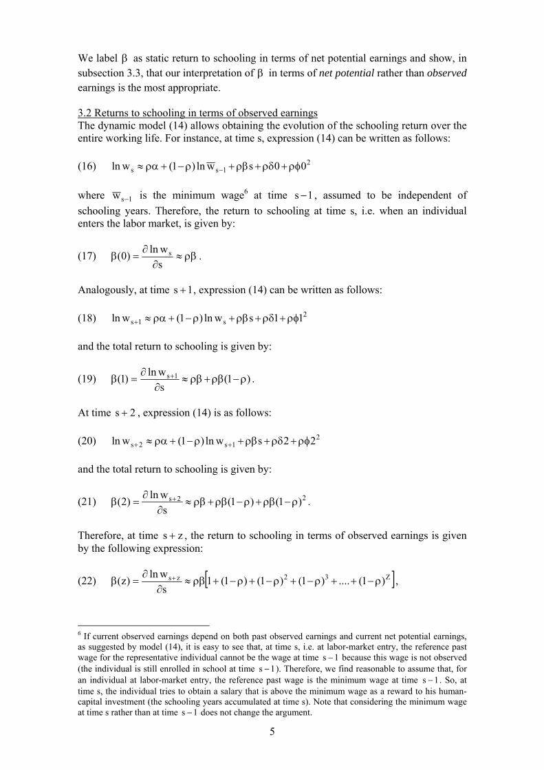
We label β as static return to schooling in terms of net potential earnings and show, in subsection 3.3, that our interpretation of β in terms of net potential rather than observed earnings is the most appropriate. 3.2 Returns to schooling in terms of observed earnings The dynamic model (14) allows obtaining the evolution of the schooling return over the entire working life. For instance, at time s, expression (14) can be written as follows: (16) 2

1ss 00swln)1(wln ρφ+ρδ+ρβ+ρ−+ρα≈ − where 1sw − is the minimum wage6 at time 1s − , assumed to be independent of schooling years. Therefore, the return to schooling at time s, i.e. when an individual enters the labor market, is given by:

(17) ρβ≈∂

∂=β

swln)0( s .

Analogously, at time 1s + , expression (14) can be written as follows: (18) 2

s1s 11swln)1(wln ρφ+ρδ+ρβ+ρ−+ρα≈+ and the total return to schooling is given by:

(19) )1(swln)1( 1s ρ−ρβ+ρβ≈∂

∂=β + .

At time 2s + , expression (14) is as follows: (20) 2

1s2s 22swln)1(wln ρφ+ρδ+ρβ+ρ−+ρα≈ ++ and the total return to schooling is given by:

(21) 22s )1()1(swln)2( ρ−ρβ+ρ−ρβ+ρβ≈∂

∂=β + .

Therefore, at time zs + , the return to schooling in terms of observed earnings is given by the following expression:

(22) [ ]Z32zs )1(....)1()1()1(1swln)z( ρ−++ρ−+ρ−+ρ−+ρβ≈∂

∂=β + ,

6 If current observed earnings depend on both past observed earnings and current net potential earnings, as suggested by model (14), it is easy to see that, at time s, i.e. at labor-market entry, the reference past wage for the representative individual cannot be the wage at time 1s − because this wage is not observed (the individual is still enrolled in school at time 1s − ). Therefore, we find reasonable to assume that, for an individual at labor-market entry, the reference past wage is the minimum wage at time 1s − . So, at time s, the individual tries to obtain a salary that is above the minimum wage as a reward to his human-capital investment (the schooling years accumulated at time s). Note that considering the minimum wage at time s rather than at time 1s − does not change the argument.

6

and is, in general, dependent of labor-market experience z. Clearly, at the end of the working life, the total return in terms of observed earnings is as follows:

(23) [ ]T32Ts )1(....)1()1()1(1s

wln)T( ρ−++ρ−+ρ−+ρ−+ρβ≈∂

∂=β + .

3.3 Dynamic return to schooling in terms of net potential earnings The return in expression (22) is, in general, lower than the return in expression (15), although the first converges to the latter as labor-market experience z increases. Indeed, for a value of )1,0(∈ρ , the following expression holds:

(24) ⎥⎦

⎤⎢⎣

⎡ρ−−

ρβ≈β=∞β∞→ )1(1

1)z(lim)(z

.

Therefore, the dynamic model (14) is able to provide a measure of β comparable7 with expression (15). We label )(∞β as dynamic return to schooling in terms of net potential earnings. Expression (24) helps to show that our interpretation of β in terms of net potential rather than observed earnings is the most appropriate because nobody can live and work forever. To the extent of T being a finite number, the return to schooling in terms of observed earnings )z(β can never be equal to β , but in the very special case of 1=ρ . 3.4 Final remarks It is easy to prove that the following inequalities hold: (25) β<β<β<β )T()z()0( for every z and T such that ∞<<< Tz0 and 0>β , if )1,0(∈ρ . In addition, one can verify that: (26) β<=β=β=β 0)T()z()0( for every z and T such that ∞<<< Tz0 and 0>β , if 0=ρ . Finally, it is easy to show that: (27) β=β=β=β )T()z()0( for every z and T such that ∞<<< Tz0 and 0>β , if 1=ρ . 3.5 Numerical example As a matter of example, we use the adjustment model (14) to compute returns to schooling in terms of both potential and observed earnings using our preferred estimates in Table 1 (GMM-SYS, controlling for year effects).

7 Note that β=⎥

⎦

⎤⎢⎣

⎡ρ−−

ρβ)1(1

1 .

7

Using expression (24), it is easy to calculate that the return to schooling in terms of potential earnings )(∞β , the equivalent of the static β return in the standard Mincer model (11), is equal to 0.053, 0.089 and 0.093 in Denmark, Finland and Belgium, respectively. In addition, we can use expression (22) to calculate the average return to schooling in terms of observed earnings over the working life )z(β . As shown in Figure 1 (the horizontal axis measures potential labor-market experience z), the standard static Mincerian model would not capture the fact that the return to schooling is increasing over time at the beginning of the working life and that the actual return to schooling at labor-market entry )0(β (estimated at 0.031, 0.062 and 0.070 in Denmark, Belgium and Finland, respectively) may be well below the potential one ( )(∞β ). Since a dynamic version of the Mincer equation seems sufficiently robust on the empirical ground, the next step consists of discussing its possible theoretical foundations. Specifically, the next section shows that a dynamic Mincer equation can be obtained as the solution of a simple wage-bargaining model. 4. Bargaining model From a theoretical point of view, assumption (10) fits within the perfect-competition framework where the nominal wage equals the monetary value of the marginal labor productivity. However, if one believes that the imperfect-competition framework is a more realistic view of the labor market8, then several arguments can support the statement that assumption (10) is unlikely to hold. This section focuses on one of the possible arguments: the existence of wage bargaining at worker-employer level. Additional arguments (asymmetric information, role of unions and efficiency wages) are briefly discussed in the last section of this paper. The standard Mincerian model puts emphasis on the supply side: the more an individual invests in his human-capital development, the higher his wage is. The model that is presented in this section aims at enhancing the role played by demand factors in determining wages, without diminishing the one played by supply factors. More explicitly, the argument is that schooling and post-schooling investments provide individuals with net potential earnings, meaning skills required to earn a given amount of money. However, observed earnings are likely to be the result of both worker’s skills (supply) and employer’s willingness to pay (demand). Since real-life labor markets are characterized by wage bargaining, the possibility of a margin-formation between observed earnings and net potential earnings should not be ruled out a-priori. This implies that observed earnings may not coincide with net potential earnings at any time, although the former generally depend on the latter. As additional feature, the model keeps into account the stylized fact that observed earnings exhibit path-dependence (persistence). To the best of our knowledge, this feature is novel because the existing (micro and macro) evidence on the autoregressive nature of observed earnings9 has not received attention in Mincerian studies so far. To anticipate the model’s conclusion, current observed earnings are shown to be dependent on both past observed earnings and current net potential earnings. Let us assume that the logarithm of the observed earnings of a worker arises from a simple, decentralized Nash bargaining between a worker and an employer and that:

8 A general reference is the New Keynesian view of the labor market. 9 See Taylor (1999) for a good survey.

8

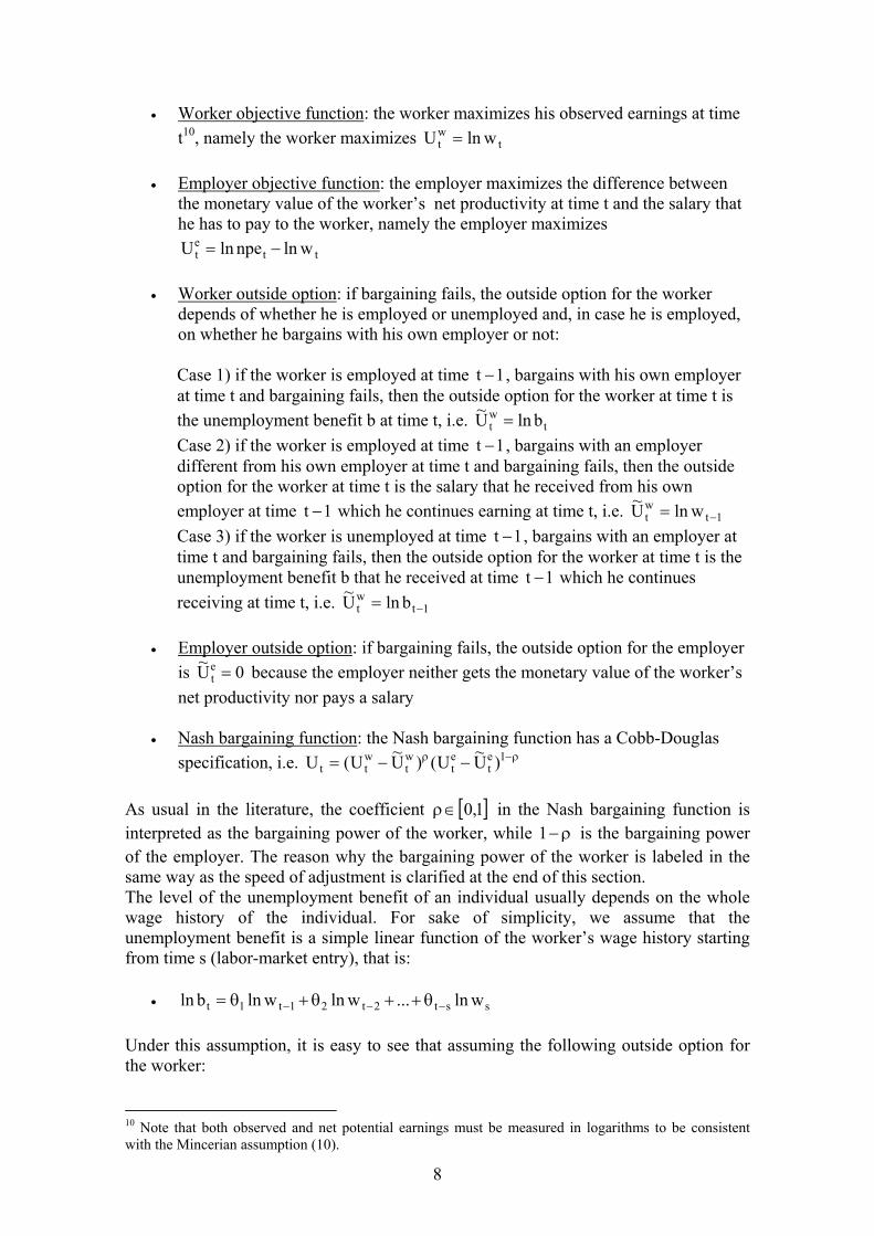
• Worker objective function: the worker maximizes his observed earnings at time

t10, namely the worker maximizes twt wlnU =

• Employer objective function: the employer maximizes the difference between

the monetary value of the worker’s net productivity at time t and the salary that he has to pay to the worker, namely the employer maximizes

ttet wlnnpelnU −=

• Worker outside option: if bargaining fails, the outside option for the worker

depends of whether he is employed or unemployed and, in case he is employed, on whether he bargains with his own employer or not:

Case 1) if the worker is employed at time 1t − , bargains with his own employer at time t and bargaining fails, then the outside option for the worker at time t is the unemployment benefit b at time t, i.e. t

wt blnU~ =

Case 2) if the worker is employed at time 1t − , bargains with an employer different from his own employer at time t and bargaining fails, then the outside option for the worker at time t is the salary that he received from his own employer at time 1t − which he continues earning at time t, i.e. 1t

wt wlnU~ −=

Case 3) if the worker is unemployed at time 1t − , bargains with an employer at time t and bargaining fails, then the outside option for the worker at time t is the unemployment benefit b that he received at time 1t − which he continues receiving at time t, i.e. 1t

wt blnU~ −=

• Employer outside option: if bargaining fails, the outside option for the employer

is 0U~ et = because the employer neither gets the monetary value of the worker’s

net productivity nor pays a salary

• Nash bargaining function: the Nash bargaining function has a Cobb-Douglas specification, i.e. ρ−ρ −−= 1e

tet

wt

wtt )U~U()U~U(U

As usual in the literature, the coefficient [ ]1,0∈ρ in the Nash bargaining function is interpreted as the bargaining power of the worker, while ρ−1 is the bargaining power of the employer. The reason why the bargaining power of the worker is labeled in the same way as the speed of adjustment is clarified at the end of this section. The level of the unemployment benefit of an individual usually depends on the whole wage history of the individual. For sake of simplicity, we assume that the unemployment benefit is a simple linear function of the worker’s wage history starting from time s (labor-market entry), that is:

• sst2t21t1t wln...wlnwlnbln −−− θ++θ+θ= Under this assumption, it is easy to see that assuming the following outside option for the worker: 10 Note that both observed and net potential earnings must be measured in logarithms to be consistent with the Mincerian assumption (10).

9

• sst2t21t1wt wln...wlnwlnU~ −−− θ++θ+θ=

takes into account all the three cases described above. Case 1) is trivially included. Case 2) holds when 11 =θ and 0i =θ for st,...,2i −= . Case 3) holds when 01 =θ and

0i ≠θ for st,...,2i −= . The solution of the worker-employer bargaining problem provides the following first-order condition:

(28) ttsst2t21t1t wlnnpeln

1wln...wlnwlnwln −

ρ−=

θ−−θ−θ−ρ

−−−

which, in turn, yields: (29) tsst2t21t1t npelnwln)1(...wln)1(wln)1(wln ρ+θρ−++θρ−+θρ−= −−− Hence, if the worker has full bargaining power ( 1=ρ ), then expression (29) becomes expression (10) and the standard Mincerian model holds. Intuitively, only when the worker has full bargaining power, he is actually able to earn all his net potential earnings. In this case, the employer is indifferent between employing and not employing because 0U~U e

tet == .

On the other hand, if the worker has zero bargaining power ( 0=ρ ), then expression (29) implies sst2t21t1t wln...wlnwlnwln −−− θ++θ+θ= . In this case, the worker is

indifferent between working and being unemployed because wt

wt U~U = .

In general, when the bargaining power of the worker is neither null nor full ( 10 <ρ< ), replacing expression (9) into (29) yields: (30) ( )2

sst2t21t1t zzswln)1(...wln)1(wln)1(wln φ+δ+β+αρ+θρ−++θρ−+θρ−≈ −−− or alternatively: (31) 2

432sst2t21t10t zzswln)1(...wln)1(wln)1(wln υ+υ+υ+θρ−++θρ−+θρ−+υ≈ −−− where the all the υ coefficients are those defined in section 2. Note that, under case 2) hypotheses i.e. 11 =θ and 0i =θ for st,...,2i −= , model (31) and model (14) perfectly match. Therefore, in case 2), the bargaining power of the worker can be interpreted as a proxy of the speed of adjustment and vice-versa. Specifically, the fact that the speed is far from being one indicates that the bargaining power of the worker is far from being full and vice-versa. Model (31), as it is, cannot be estimated with usually available panel data because it requires information about the whole wage history of each individual in the dataset, typically not available. However, standard longitudinal datasets usually allow to test for the significance of wage lags up to a certain point in the past. Using our dataset, we are able to test several possibilities and find that the most appropriate specification of model (31) for Belgium and Finland has two significant wage lags while, for Denmark, it has just one lagged wage. Additional wage lags are not statistically significant. An important issue to be taken into account before estimating model (31) is that the model can only be applied to countries where unemployment benefits are actually paid and cover a large share of the working force. To this respect, we would like to stress

10

that Boeri and van Ours (2008, p. 283) indicate Belgium, Finland and Denmark as the countries with the highest generosity index of unemployment benefit adjusted for coverage in a sample of 12 European countries. Besides issues of data availability with other countries, the latter is the main reason why these three countries have been chosen for the empirical analysis in this paper. Note that the number of relevant wage lags (also called wage persistence) may depend on the specific way the unemployment-benefit policies are designed in a given country (duration, eligibility, administrative rules regarding the determination of the benefit level, and so on). As a matter of example, it may be the case that i) recent earnings are relatively more important than older earnings for the determination of the benefit level, or that ii) just the most recent wages really matter for the benefit. This would imply that some of the θ coefficients in the simple benefit-determination rule assumed in the bargaining model may be either i) not statistically different from zero or ii) zero by assumption. For instance, if 0i =θ for st,...,3i −= , then model (31) would just have two relevant lagged wages. In addition, the number of relevant wage lags may also depend on the proportion of case 1), case 2) and case 3) workers in the dataset. For instance, if just case 2) workers were in the dataset, model (31) would suggest that just one lag of the hourly wage should be significant because the outside option of the worker would just be that of case 2). The significance of more than one lag may be seen as indication that case 1) and case 3) workers are significantly represented in the dataset. Of course, many other country-level aspects related to labor-market institutions and legislation may also explain different degrees of wage persistence. For instance, if the share of temporary contracts relative to permanent contracts is higher in country A relative to country B, this may imply a higher number of bargaining processes among workers and employers taking place in country A and may affect the persistence of wages in country A relative to B. Alternatively, if firing is more costly or difficult in country B, this would imply a different outside option of the worker in country B relative to A and may affect the relative degree of wage persistence in the two countries. Table 2 presents our GMM-SYS estimates based on model (31), controlling for endogeneity, individual heterogeneity and year effects. All standard tests are passed and their results indicate a specification improvement for Belgium, no real gain with respect to the adjustment model for Denmark, some mixed evidence for Finland where the second wage lag is significant but the Hansen J test does not significantly improve and the 2nd order autocorrelation test shows a lower p-value. The main conclusion is that a micro-founded dynamic wage model, the bargaining model, can fit the data better than a simple adjustment model but requires more (sometimes non-testable) theoretical assumptions. 5. Conclusions The main conclusions of this paper are the following:

a. The equality between the observed wage of an individual and the monetary value of his net human-capital productivity (the so-called net potential wage), assumed by the standard Mincerian model, is rejected by the ECHP data for Belgium, Denmark and Finland

b. A dynamic approach to the Mincer equation based on a simple wage adjustment

model implies that the return to schooling in terms of observed earnings is not independent of labor-market experience

11

c. The return to schooling in terms of net potential earnings, provided by the standard Mincer equation, can also be computed using a dynamic wage adjustment model

d. A dynamic adjustment model allows the estimation of the average return to

schooling at labor-market entry

e. A dynamic wage equation can be seen as the solution of a simple wage bargaining model where the role played by demand factors is enhanced with respect to the standard supply-side Mincerian framework

f. A micro-founded dynamic wage model, the bargaining model, can fit the data

better than a simple adjustment model but requires more theoretical assumptions The rest of this section discusses the above results in the light of the existing literature on human-capital wage equations, with special emphasis on result b. which we consider the most important (although it is a consequence of result a.) The seminal book by Mincer (1974) has been the starting point of a large body of literature dealing with the estimation of a wage equation where the logarithm of the hourly wage of an individual is explained by his schooling years, potential labor-market experience, and experience squared. Within this framework, the coefficient of schooling years is usually interpreted as being the return to an additional year of schooling in terms of observed earnings. An excellent synthesis of the research papers adopting the Mincer equation as underlying framework has been provided by Card (1999). The reviewed works generally focused on the estimation of the average impact of schooling on earnings, by means of both OLS and instrumental-variable techniques. Today, ‘the state of the art’ described by Card looks outdated. This is partly because the last decade was characterized by a special interest in adopting the Mincer equation for identifying the effect of schooling not only on the mean but also on the shape of the conditional wage distribution, using the quantile-regression techniques due to Koenker and Bassett (1978). Starting from a seminal work by Buchinsky (1994), the last few years saw the publication of numerous estimates of the schooling coefficient along the conditional wage distribution, with the frequent finding that education has a positive impact on within-groups wage inequality, as suggested by Martins and Pereira (2004) among others. Additional results using instrumental-variable techniques for quantile regression have been provided by Arias et al. (2001), Chernozhukov and Hansen (2006), Lee (2007), Andini (2008), and many others. In spite of its wide acceptance within the profession, the spread of the framework developed by Mincer over the last forty years has not been uncontroversial. Some authors criticized the Mincerian framework by arguing that the framework is not able to provide a good fit of empirical data; some stressed that the average effect of schooling on earnings is likely to be non-linear in schooling; some suggested that education levels should replace schooling years in the wage equation. For instance, Murphy and Welch (1990) maintained that the standard Mincer equation provides a very poor approximation of the true empirical relationship between earnings and experience, while Trostel (2005) argued that the average impact of an additional year of schooling on earnings varies with the number of completed schooling years. In summary, there have been some critical voices but, looking at the big picture, we must reasonably conclude that the history of human-capital regressions has been characterized by a generalized attempt of consistently estimating the coefficient of

12

schooling (both on average and along the conditional wage distribution), under an implicit acceptance of the theoretical interpretation of the schooling coefficient itself. Nevertheless, the important issue of the theoretical interpretation of the schooling coefficient has been recently rediscovered by Heckman et al. (2005), who empirically tested several implications of the classical Mincerian framework, using Census data for the United States. Among other implications of the Mincerian approach, the authors tested and often rejected the implication that the return to schooling in terms of observed earnings is independent of labor-market experience. On the lines of Heckman et al. (2005), our paper has provided additional theoretical and empirical arguments against the usual interpretation of the coefficient of schooling in the standard Mincer equation. Indeed, we have argued that the return to schooling in terms of observed earnings is, in general, dependent of labor-market experience (result b.). This result is also consistent with more recent empirical evidence provided Belzil (2007) and with some earlier evidence presented by Andini (2005)11. As shown, the result b. can be easily derived from a dynamic specification of the Mincer equation where past observed earnings contribute to explain current observed earnings. This specification is strongly supported by the ECHP data for three European countries, once endogeneity, individual heterogeneity and time effects are accounted for (result a.), and allows to compute the return to schooling at labor-market entry (result d.) as well as the standard Mincerian return to schooling (result c.). This paper also provides a theoretical micro-foundation of a dynamic Mincer equation, where demand factors are considered as important as supply factors for wage determination (result e.). It is worth stressing that, of course, we do not claim for generality. Clearly, the bargaining model in section 4 holds under a set of specific assumptions. The main issue, at this point, is whether these assumptions bring us closer to reality (enhanced role of demand factors in determining wages) or not. The bargaining model is presented here as a micro-founded alternative to the simple adjustment model. The former can perform better than the latter in terms of data fitting because it allows for more than one wage lag but it is based on more theoretical hypotheses (result f.) and, as it stands, it is only suitable to be used for countries where unemployment benefits are actually paid and cover a large share of the working force. Summing up, to really conclude this paper, we would like to stress that there seems to be substantial empirical evidence supporting the argument that past observed earnings, together with accumulated human capital (schooling and post-schooling investments), play an important role in explaining current observed earnings. This finding should open the door to new research efforts looking for alternative, and perhaps more general, theoretical foundations of a dynamic Mincer equation. Issues related to asymmetric information (for instance, the case where the employer does not observe the net potential earnings of the worker), role of unions (wage bargaining at collective level and insider-outsider considerations) and efficiency wages (the employer cannot observe the worker’s effort) are interesting topics for future investigation.

11 Some of the ideas that are presented in this paper can also be found in Andini (2007), Andini (2009) and Andini (forthcoming). However, these works do not control for endogeneity, individual heterogeneity and time effects in the estimation of the dynamic Mincer equation.

13

References Andini C. (2005) Returns to Schooling in a Dynamic Model, CEEAplA Working Papers, nº 4, Centre of Applied Economic Studies of the Atlantic. Andini C. (2007) Returns to Education and Wage Equations: A Dynamic Approach, Applied Economics Letters, 14(8): 577-579. Andini C. (2008) The Total Impact of Schooling on Within-Groups Wage Inequality in Portugal, Applied Economics Letters, 15(2): 85-90. Andini C. (2009) Wage Bargaining and the (Dynamic) Mincer Equation, Economics Bulletin, 29(3): 1846-1853. Andini C. (forthcoming) A Dynamic Mincer Equation with an Application to Portuguese Data, Applied Economics, DOI: 10.1080/00036840701765429. Arellano M., Bond S. R. (1991) Some Tests of Specification for Panel Data: Monte Carlo Evidence and an Application to Employment Equations, Review of Economic Studies, 58(2): 277–297 Arias O., Hallock K.F., Sosa-Escudero W. (2001) Individual Heterogeneity in the Returns to Schooling: Instrumental Variables Quantile Regression Using Twins Data, Empirical Economics, 26(1): 7-40. Belzil C. (2007) Testing the Specification of the Mincer Equation, IZA Discussion Papers, nº 2650, Institute for the Study of Labor. Blundell R.W., Bond S. R. (1998) Initial Conditions and Moment Restrictions in Dynamic Panel Data Models, Journal of Econometrics, 87(1): 115–143 Boeri T., van Ours J. (2008) The Economics of Imperfect Markets, Princeton NJ: Princeton University Press. Buchinsky M. (1994) Changes in the U.S. Wage Structure 1963-1987: Application of Quantile Regression, Econometrica, 62(2): 405-458. Card D. (1999) The Causal Effect of Education on Earnings, in: Ashenfelter O., Card D. (Eds.) Handbook of Labor Economics, New York: North Holland. Chernozhukov V., Hansen C. (2006) Instrumental Quantile Regression Inference for Structural and Treatment Effect Models, Journal of Econometrics, 132(2): 491-525. Connolly H., Gottschalk P. (2006) Differences in Wage Growth by Education Level: Do Less-Educated Workers Gain Less from Work Experience?, IZA Discussion Papers, nº 2331, Institute for the Study of Labor. Flannery M.J., Rangan K.P. (2006) Partial Adjustment toward Target Capital Structures, Journal of Financial Economics, 79(3): 469-506. Heckman J.J, Lochner L.J., Todd P.E. (2003) Fifty Years of Mincer Earnings Regressions, NBER Working Papers, nº 9732, National Bureau of Economic Research.

14

Heckman J.J., Lochner L.J., Todd P.E. (2005) Earnings Functions, Rates of Return, and Treatment Effects: the Mincer Equation and Beyond, NBER Working Papers, nº 11544, National Bureau of Economic Research. Koenker R., Bassett G. (1978) Regression Quantiles, Econometrica, 46(1): 33-50. Krueger A.B., Lindahl M. (2001) Education for Growth: Why and for Whom?, Journal of Economic Literature, 39(4): 1101-1136. Lee S. (2007) Endogeneity in Quantile Regresssion Models: A Control Function Approach, Journal of Econometrics, 141(2): 1131-1158. Martins P.S., Pereira P.T. (2004) Does Education Reduce Wage Inequality? Quantile Regression Evidence from 16 Countries, Labour Economics, 11(3): 355-371. Mincer J. (1974) Schooling, Experience and Earnings, Cambridge MA: National Bureau of Economic Research. Murphy K.M., Welch F. (1990) Empirical Age-Earnings Profiles, Journal of Labor Economics, 8(2): 202-229. Rubinstein Y., Weiss Y. (2006) Post Schooling Wage Growth: Investment, Search and Learning, in: Hanushek E.A., Welch F. (Eds.) Handbook of the Economics of Education, New York: North Holland. Taylor J.B. (1999) Staggered Price and Wage Setting in Macroeconomics, in: Taylor J.B., Woodford M. (Eds.) Handbook of Macroeconomics, New York: North Holland. Trostel P.A. (2005) Nonlinearity in the Return to Education, Journal of Applied Economics, 8(1): 191-202.

15

Table 1. Adjustment model

Dependent variable: Logarithm of gross hourly wage Belgium Denmark Finland 1994-2001 1994-2001 1996-2001 OLS Constant 1.223 (0.000) 0.983 (0.000) 1.193 (0.000) Logarithm of gross hourly wage (-1) 0.757 (0.000) 0.775 (0.000) 0.627 (0.000) Schooling years 0.016 (0.000) 0.009 (0.000) 0.023 (0.000) Potential labor-market experience 0.005 (0.001) 0.001 (0.562) 0.007 (0.018) Potential labor-market experience squared -0.000 (0.168) -0.000 (0.787) -0.000 (0.288) OLS, controlling for year effects Constant 1.252 (0.000) 0.948 (0.000) 1.179 (0.000) Logarithm of gross hourly wage (-1) 0.754 (0.000) 0.772 (0.000) 0.624 (0.000) Schooling years 0.016 (0.000) 0.010 (0.000) 0.025 (0.000) Potential labor-market experience 0.006 (0.000) 0.002 (0.493) 0.008 (0.014) Potential labor-market experience squared -0.000 (0.094) -0.000 (0.684) -0.000 (0.308) GMM-SYS Constant 2.102 (0.000) 1.740 (0.000) 2.005 (0.000) Logarithm of gross hourly wage (-1) 0.443 (0.000) 0.543 (0.000) 0.305 (0.016) Schooling years 0.073 (0.000) 0.017 (0.001) 0.051 (0.000) Potential labor-market experience 0.022 (0.000) 0.027 (0.003) 0.016 (0.126) Potential labor-market experience squared -0.000 (0.116) -0.000 (0.011) -0.000 (0.725) Arellano-Bond 1st order autocorr. test (p-value) (0.000) (0.001) (0.029) Arellano-Bond 2nd order autocorr. test (p-value) (0.065) (0.041) (0.510) Hansen J overid. test (p-value) (0.030) (0.552) (0.006) GMM-SYS, controlling for year effects Constant 2.901 (0.000) 2.145 (0.000) 2.109 (0.000) Logarithm of gross hourly wage (-1) 0.335 (0.000) 0.420 (0.000) 0.218 (0.085) Schooling years 0.062 (0.000) 0.031 (0.000) 0.070 (0.000) Potential labor-market experience 0.032 (0.000) 0.028 (0.006) 0.014 (0.188) Potential labor-market experience squared -0.000 (0.000) -0.000 (0.023) 0.000 (0.922) Arellano-Bond 1st order autocorr. test (p-value) (0.000) (0.001) (0.033) Arellano-Bond 2nd order autocorr. test (p-value) (0.121) (0.117) (0.493) Hansen J overid. test (p-value) (0.256) (0.738) (0.127)

P-values of estimated coefficients, in parentheses, are based on White-corrected standard errors for OLS and on Windmeijer-corrected standard errors for GMM-SYS. GMM-SYS estimates are based on the xtabond2 module for Stata and the following instruments sets:

Instruments for first differences equation a) Standard: first differences of the time dummies b) GMM-type: lagged values of all the regressors excluding time dummies from the beginning of

the sample to 2t − Instruments for levels equation c) Standard: constant d) GMM-type: lagged values of the first differences of all the regressors excluding time dummies

16

Table 2. Bargaining model

Dependent variable: Logarithm of gross hourly wage Belgium Denmark Finland 1994-2001 1994-2001 1996-2001 GMM-SYS, controlling for year effects Constant 1.607 (0.000) 2.648 (0.000) 1.316 (0.003) Logarithm of gross hourly wage (-1) 0.511 (0.000) 0.409 (0.000) 0.296 (0.050) Logarithm of gross hourly wage (-2) -0.130 (0.000) -0.092 (0.324) 0.228 (0.001) Schooling years 0.033 (0.002) 0.032 (0.000) 0.043 (0.023) Potential labor-market experience 0.016 (0.002) 0.026 (0.073) 0.010 (0.266) Potential labor-market experience squared -0.000 (0.048) -0.000 (0.144) 0.000 (0.794) Arellano-Bond 1st order autocorr. test (p-value) (0.000) (0.000) (0.136) Arellano-Bond 2nd order autocorr. test (p-value) (0.978) (0.407) (0.262) Hansen J overid. test (p-value) (0.730) (0.682) (0.145)

P-values of estimated coefficients, in parentheses, are based on Windmeijer-corrected standard errors. GMM-SYS estimates are based on the xtabond2 module for Stata and the following instruments sets:

Instruments for first differences equation a) Standard: first differences of the time dummies b) GMM-type: lagged values of all the regressors excluding time dummies from the beginning of

the sample to 2t − Instruments for levels equation c) Standard: constant d) GMM-type: lagged values of the first differences of all the regressors excluding time dummies

17

Figure 1. Returns to schooling in terms of observed earnings )z(β

Belgium

0.0000.0100.0200.0300.0400.0500.0600.0700.0800.0900.100

0 5 10 15 20 25 30 35 40 45

Belgium: 062.0)0( =β and 093.0)( =∞β

Denmark

0.0000.0100.0200.0300.0400.0500.0600.0700.0800.0900.100

0 5 10 15 20 25 30 35 40 45

Denmark: 031.0)0( =β and 053.0)( =∞β

Finland

0.0000.0100.0200.0300.0400.0500.0600.0700.0800.0900.100

0 5 10 15 20 25 30 35 40 45

Finland: 070.0)0( =β and 089.0)( =∞β

18

Appendix. Sample descriptive statistics Our data are extracted from the European Community Household Panel. We focus on male workers aged between 18 and 65. In order to derive the variables for schooling years (ys), potential labour-market experience (plme) and the logarithm of the gross hourly wage (lnw), we use the following ECHP variables:

• pt023. Age when the highest level of general or higher education was completed • pe039. How old were you when you began your working life, that is, started your first job or

business? • pd003. Age • pi211mg. Current wage and salary earnings – gross (monthly) • pe005. Total number of hours per week (in main + additional jobs)

Specifically, to be consistent with the standard Mincerian model (the representative agent first stops schooling and then starts working), we select a sample of individuals whose age at the completion of the highest level of education was lower than their age at the start of the working life (pt023 ≤ pe039) and define the above-referred variables as follows:

• ys = pt023 – 6 (def.1) • plme = pd003 – ys – 6 (def. 2)

It is worth stressing that ys numbers do not necessarily reflect successfully completed years of schooling. This is a compromise that allows us to obtain homogenous measures of schooling years (and potential labour-market experience) across three countries that are different in many aspects including educational systems. The variable lnw represents the natural logarithm of the individual gross hourly wage. From the gross monthly wage (pi211mg), we obtain the daily (dividing the monthly wage by 30) and the weekly wage (multiplying the daily wage by 7). Dividing the latter by the number of weekly hours of work (pe005), we obtain the hourly wage. Belgium, 1994-2001 Variable Obs. Mean Std. Dev. Min Max lnw 6873 6.164 0.433 2.815 8.697 ys 6873 13.858 3.240 4 25 plme 6873 19.521 10.362 0 51 Denmark, 1994-2001 Variable Obs. Mean Std. Dev. Min Max lnw 2053 4.811 0.521 -0.326 6.368 ys 2053 14.943 4.592 6 29 plme 2053 17.173 11.486 0 52 Finland, 1996-2001 Variable Obs. Mean Std. Dev. Min Max lnw 2341 4.256 0.509 -0.405 7.522 ys 2341 15.423 3.355 5 27 plme 2341 14.800 9.999 0 46