DI

SC

US

SI

ON

P

AP

ER

S

ER

IE

S

Forschungsinstitut zur Zukunft der ArbeitInstitute for the Study of Labor

Using the Helmert-Transformation to Reduce Dimensionality in a Mixed Model: Application to a Wage Equation with Worker and Firm Heterogeneity

IZA DP No. 5847

July 2011

Øivind A. NilsenArvid RaknerudTerje Skjerpen

Using the Helmert-Transformation to Reduce Dimensionality in a Mixed Model:

Application to a Wage Equation with Worker and Firm Heterogeneity

Øivind A. Nilsen Norwegian School of Economics

and IZA

Arvid Raknerud Statistics Norway

Terje Skjerpen

Statistics Norway

Discussion Paper No. 5847

July 2011

IZA

P.O. Box 7240 53072 Bonn

Germany

Phone: +49-228-3894-0 Fax: +49-228-3894-180

E-mail: iza@iza.org

Any opinions expressed here are those of the author(s) and not those of IZA. Research published in this series may include views on policy, but the institute itself takes no institutional policy positions. The Institute for the Study of Labor (IZA) in Bonn is a local and virtual international research center and a place of communication between science, politics and business. IZA is an independent nonprofit organization supported by Deutsche Post Foundation. The center is associated with the University of Bonn and offers a stimulating research environment through its international network, workshops and conferences, data service, project support, research visits and doctoral program. IZA engages in (i) original and internationally competitive research in all fields of labor economics, (ii) development of policy concepts, and (iii) dissemination of research results and concepts to the interested public. IZA Discussion Papers often represent preliminary work and are circulated to encourage discussion. Citation of such a paper should account for its provisional character. A revised version may be available directly from the author.

IZA Discussion Paper No. 5847 July 2011

ABSTRACT

Using the Helmert-Transformation to Reduce Dimensionality in a Mixed Model: Application to a

Wage Equation with Worker and Firm Heterogeneity* A model for matched data with two types of unobserved heterogeneity is considered – one related to the observation unit, the other to units to which the observation units are matched. One or both of the unobserved components are assumed to be random. This mixed model allows identification of the effect of time-invariant variables on the observation units. Applying the Helmert transformation to reduce dimensionality simplifies the computational problem substantially. The framework has many potential applications; we apply it to wage modeling. Using Norwegian manufacturing data shows that the assumption with respect to the two types of heterogeneity affects the estimate of the return to education considerably. JEL Classification: C23, C81, J31 Keywords: high-dimensional two-way unobserved components, matched employer-employee data, ECM-algorithm Corresponding author: Arvid Raknerud Statistics Norway PO Box 8131 Dep NO-0033 Oslo Norway E-mail: rak@ssb.no

* Comments and suggestions made during the presentation at the Nordic Econometric Meeting 2011, and on a previous version of this paper at ESEM 2009 in Barcelona are greatly appreciated.

1 Introduction

Access to matched data sets enables consideration of unobserved heterogeneity cor-

responding to di¤erent types of units in regression analyses. Often the main focus

is on one type of observational unit, but it is also necessary to account for unob-

served heterogeneity caused by another type of observational unit that is matched

to the main type. Wage modeling by means of matched employer�employee data,

which is the topic of the current paper, may be the best-known example. Here, the

individual is considered the main observational unit, whereas the �rm to which the

individual is matched has the role of a secondary observational unit. For consistent

and e¢ cient estimation of the e¤ects of observed explanatory variables it is vital to

account for both individual- and �rm-speci�c unobserved heterogeneity. Using only

individual-level data may yield misleading policy implications.

However, other �elds in economics may have a corresponding data design. Let us

mention three examples, which we do not claim are exhaustive. If there are matched

data for banks and their customers, one may account for both unobserved bank and

bank customer-speci�c e¤ects.1 A second example could be connected to FDI. A

domestic �rm is matched to a foreign country, and it is desirable to account for

unobserved heterogeneity stemming both from the �rm itself and from the country

in which the �rm is involved.2 A �nal example is taken from health economics

in a modeling framework where the main observational unit consists of patients

and where they are matched to general practitioners. With such data, unobserved

heterogeneity related both to the patients and to the general practitioners may be

considered.3

Returning to wage modeling, Abowd et al. (1999), whose paper constitutes a

1For instance, this is the case in Ioannidou and Ongena (2010).2For an overview of analyses of FDI in a panel data context, see Blanchard et al. (2008).3For a panel data analysis employing matched data of this type, see for instance Godager and

Biørn (2010).

2

seminal contribution with respect to wage modeling using employer�employee data,

represented both unobserved individual- and �rm-speci�c heterogeneity by �xed

e¤ects. In applications, the researcher is often interested in the e¤ect of observed

time-invariant variables, or of variables that may almost be regarded as such. An

example is the length of education, which for most individuals does not vary over

the sample period. However, the �xed e¤ects speci�cation has the problematic

feature that one cannot identify the e¤ects of variables that are constant over time.

For example, the e¤ect of a change in education is identi�ed when the individual

e¤ects are random, but not when they are �xed.4 Another advantage of the random

components model is that it is far more parsimonious with respect to the number

of parameters than the �xed e¤ects model.

In this paper, we consider a linear mixed model with an unobserved e¤ect corre-

sponding to the main observation unit (e.g., an individual) and an unobserved e¤ect

corresponding to another type of unit (e.g., a �rm) with which the main observation

unit is matched at a given point in time.5 The matching between the two types of

units may change over time, and is considered to be the outcome of an exogenous

matching variable. We allow the unobserved e¤ects corresponding to the matched

units to be correlated. Before estimating the parameters of the regression equation

we apply the Helmert transformation to reduce the dimensionality problem associ-

ated with a possibly very large number of latent variables.6 The main contribution

of this paper is to show that, within a random e¤ects framework, the Helmert trans-

4There may also be intermediate cases in a situation with several covariates when it is possibleto identify the e¤ect of one-dimensional variables even in the presence of �xed e¤ects. However,this requires an a priori assumption stating that some of the covariates are uncorrelated with therandom unobserved individual-speci�c term. For this approach, cf. Hausman and Taylor (1981).

5For the statistical treatment of linear mixed models, cf. for instance Searle et al. (1992) andDemidenko (2004).

6Balestra and Krishnakumar (2008) and Arellano and Bover (2005) comment on this transfor-mation even though they do not use the label Helmert transformation. Rather, they refer to it asthe backward and forward orthogonal deviations operator. See Keane and Runkle (1992) for therelated concept of forward �ltering.

3

formation can be used to sweep out the random e¤ects corresponding to the main

observation unit. The resulting pro�le likelihood will then have much fewer latent

variables than the original model, that is, equal to the number of main units plus the

number of units to which these units can be matched. To estimate the parameters of

the models we propose an Expectation Conditional Maximization (ECM) algorithm

(see Meng and Rubin, 1993) to maximize the pro�le log-likelihood function.

In an application, we investigate the best speci�cation of unobserved heterogene-

ity in a wage equation when there is access to unbalanced employer�employee panel

data. What one ultimately seeks is a test corresponding to the standard Hausman

test applied in panel data models where one only addresses one-way unobserved

heterogeneity. Models that include random individual and �rm e¤ects as well as

random individual and �xed �rm e¤ects are of substantial interest� both types of

model allow for the identi�cation of the e¤ects of time-invariant individual-speci�c

variables, but the latter speci�cation is less restrictive.

We apply our modeling framework to a sample of individuals working in a tra-

ditional Norwegian manufacturing industry, production of machinery (NACE 29).

Panel employer�employee data for the years 1995�2006 are used. The �nal data con-

sist of 15,415 observations. We have 2,021 individuals and 770 �rms. As observed

individual covariates in the wage equation, we use length of education, a third-order

polynomial in experience, three dummies for type of education, a dummy for gen-

der, �ve dummies for labor market areas and 11 year dummies. Of the skill-related

variables, only those involving experience vary across both individuals and time.

Specifying both the unobserved individual-speci�c e¤ects and the �rm-speci�c

e¤ects as random e¤ects, we �nd the coe¢ cient of years of education to di¤er only

modestly from the estimate in the model with individual random e¤ects and no �rm

e¤ects. This is not very surprising. If the �rst speci�cation is valid, we know that the

4

covariance matrix of the gross error term, which is a sum of two one-dimensional

random terms and a genuine error term, will have a certain structure and that

this error term is independent of the explanatory variables. Accounting for this

structure is necessary to obtain e¢ cient estimates of the slope parameters of the wage

equation, but not to obtain consistent estimates of these parameters. Furthermore,

the estimate of the correlation coe¢ cient between the individual- and �rm-speci�c

random e¤ects is statistically di¤erent from zero. Constraining this parameter to

zero does not produce estimated slope parameters that are very di¤erent from those

obtained in the speci�cation where it is allowed to be estimated as a free parameter.

However, as emphasized by Eeckhout and Kircher (2010), it is not straightforward

to interpret such an empirical �nding. In contrast, the model speci�cation with

random individual e¤ects and �xed �rm e¤ects does produce substantially di¤erent

estimates with regard to returns to education. This model is more �exible than the

model where both the individual and �rm e¤ects are random, because the �xed �rm

e¤ects are not constrained to be independent of the explanatory variables, which

may explain the di¤erence in the parameter estimates.

The rest of the paper is organized as follows. In Section 2, we outline the general

modeling framework, introduce the Helmert transformation and present the estima-

tion algorithm. Section 3 contains an application on wage equation estimation and

discusses various speci�cations. Some concluding remarks are provided in Section

4.

2 The general model

The starting point of our analysis is the following model with a three-way structure:

yijt = xit� + zi + �i + �j + �ijt; (1)

5

where yijt is the endogenous variable for observation unit i, matched with unit

j, and observed at time t. In matched employer�employee data, j will typically

denote the �rm or employer of individual i at t, but other applications are obviously

possible; for example, i may denote a �rm and j its (main) bank (see Ioannidou and

Ongena, 2010). For speci�city, we henceforth refer to i as an individual and j as a

�rm. Then xit represents the time-varying covariates of individual i, zi represents

the time-invariant covariates, �i is a random e¤ect corresponding to individual i

(henceforth �individual e¤ect�), �j is a random e¤ect corresponding to �rm j (��rm

e¤ect�) and �ijt is a genuine error term.

The index j is assumed to be the outcome of a stochastic index function j =

J(i; t) 2 f1; 2; :::;Mg, denoting the unit matched to i at t. We assume throughout

that the distribution of �ijt does not depend on j. Then we can drop the subscript

j from yijt and �ijt, and rewrite (1) as follows:

yit = xit� + zi + �i + �J(i;t) + �it; (2)

where E(�it) = 0 and E(�2it) = ��� for all i; t. Letting � = (�1; :::;�M)

0 denote the

vector of all theM random e¤ects and Git an appropriate selection vector, such that

Git� =�J(i;t), we can write

yit = xit� + zi + �i +Git� + �it: (3)

To simplify the notation, we assume that all individuals enter the sample at t = 1

(or, equivalently, we can rede�ne t to denote the t�th observation on individual i).

We allow for unbalanced data, with unit i exiting the sample at t = Ti.

To sweep out the individual e¤ects from models with both individual and �rm

e¤ects, we propose to use the Helmert transformation. Formally, the Helmert trans-

6

formation of yit, t = 1; :::; Ti, is given by (�!y i;1; ::;�!y i;Ti�1; yi), where

~yi;t =pt=(t+ 1)

yi;t+1 � t�1

tXs=1

yi;s

!, t = 1; :::; Ti � 1;

and

yi = Ti�1

TiXs=1

yis:

A corresponding transformation can also be applied component wise to the variables

included in an arbitrary vector, say x. It is easy to check that all the correspond-

ing Helmert transformed error terms, �!� i;t and �i, are uncorrelated, given that the

original error terms, �it, are uncorrelated and homoscedastic (i.e., have constant

variance over time). Moreover, the individual e¤ects will be swept out from all the

transformed variables, except yi. Of course, the Helmert transformation is not the

only way of sweeping out the individual e¤ects (see, for example, Andrews et al.

(2008) for a discussion of the within estimator in this context), but it has the huge

advantage of preserving the orthogonality of the error terms.

Fixed individual and �rm e¤ects Let us �rst consider the estimator when

both the individual and the �rm e¤ects are �xed. The estimator is then obtained

by minimizing the quadratic form

Q(�; ; �; �) =

NXi=1

Ti(yi�xi��zi ��i�Gi�)2+(�!y ��!X���!G�)0(�!y ��!X���!G�)

with respect to (�; ; �; �), where � = (�1; ::::; �N)0, xi = Ti

�1PTis=1 xis, Gi =

Ti�1PTi

s=1Gis,

�!y = (�!y 10; :::;�!y N 0)0;

with �!y i = (�!y i;1; :::;�!y i;Ti�1)0, and

�!G = (

�!G 1

0; :::;

�!GN

0)0;

7

with�!G i = (

�!G i;1

0; :::;

�!G i;Ti�1

0)0. Note that

�!G has dimension

�PNi=1(Ti � 1)

��M

and Gi dimension N �M .

The �rst-order conditions for minimizing Q(�; ; �; �) then become

yi � xi� � zi � �i �Gi� = 0 (4)

and

z0i(yi � xi� � zi � �i �Gi�) = 0

�!G 0(�!y ��!X� ��!G�) = 0

�!X 0(�!y ��!X� ��!G�) = 0 (5)

(where we have used (4) in (5) ). To obtain identi�cation (a unique minimizer), ad-

ditional restrictions must be imposed, as discussed in detail in Abowd et al. (2002).

Independent random individual and �rm e¤ects Assume now that the vector

of the random �rm e¤ects, �, is distributed as

� � N (0; ���IM),

where IM is the identity matrix of dimensionM , and the vector of individual e¤ects,

�, is distributed as

� � N (0; ���IN).

If � and � are independent, then

yi � xi� � zi �Gi� = �i + �i � !i, i = 1; :::; N

�!y ��!X� ��!G� = �!� ; (6)

where�!� and !i are uncorrelated for all i and independent of �, with�!� � N (0; ���I),

where I is the identity matrix of dimensionPN

i=1(Ti�1), and !i � N�0; ���

�T�1i + �

��,with

8

� = ���=���. More compactly, de�ne y = (y1; :::; yN)0 and similarly (x;G) by stack-

ing xi and Gi. We can then stack �y and�!y to obtain�

�y�!y

�=

�x�!X

�� +

�z0

� +

�G�!G

�� +

�!�!�

�;

where z = (z01; :::; z0N)

0 and ! = (!1; :::; !N)0.

Let � = (�0; 0; ���; �; ���) denote all parameters to be estimated, and �(m) the

current estimate of � (in the m�th iteration of the estimation algorithm). Further-

more, let (�) = diag(T�11 +�; :::; T�1N +�). According to the EM algorithm we can

write

M(�j �(m)) =M (1)(�; ; ���; �j�(m)) +M (2)(��� j�(m)), (7)

where

M (1)(�; ; ���; �j�(m)) = �1

2

NXi=1

Ti ln��� �1

2

NXi=1

ln(1

Ti+ �)

� 12��1�� E

(NXi=1

(1

Ti+ �)�1(yi � xi� � zi �Gi�)2 jY ; �(m)

)

� 12��1�� E

���!y ��!X� ��!G��0 ��!y ��!X� ��!G�� jY ; �(m)�(8)

and

M (2)(��� j�(m)) = �N

2ln j��� j �

1

2��1�� E

n� 0�jY ; �(m)

o. (9)

In (8)�(9), the expectation is with respect to the latent variables � conditional on

the data Y , and with � evaluated at �(m). ThusM(�j�(m)) is the expected �complete

data� log-likelihood, obtained by considering � as observed random variables and

then taking the conditional expectation of this log-likelihood with respect to the

latent variables (given Y and the current parameter estimates). It is shown in

Dempster et al. (1977) that repeated maximization of M(�j �(m)) with respect to �

9

generates a sequence f�(m)g, which converges to a stationary point of the likelihood

function under very general conditions. Because M(�j �(m)) is quadratic in (�0; � 0),

to evaluate the expectations in (8)�(9) we only need to calculate the conditional

expectations

b�(�(m)) = En� jY ; �(m)o , (10)

and the conditional covariance matrix

V (�(m)) = Varn� jY ; �(m)

o. (11)

We have (see Francke et al., 2010)

V (�(m)) =���1�� IM + �

�1��

�G0(�(m))�1G+

�!G 0�!G

���1and

b�(�(m)) = ��1�� V (�(m)) h G0(�(m))�1 �!G 0i�� y

�!y

���x�!X

�� �

�z0

�

�:

Because the maximization ofM(�j �(m)) is complicated, we suggest modifying the

EM algorithm, replacing it with an Expectation Conditional Maximization (ECM)

algorithm (see Meng and Rubin, 1993). First, we maximize M(�j�(m)) w.r.t. � and

given � = �(m). The �rst-order conditions are given by

NXi=1

z0i(T�1i + �(m))�1

�y � xi�(m+1) � zi (m+1) �Gb�(�(m))� = 0

NXi=1

xi0(T�1i + �(m))�1

�y � xi�(m+1) � zi (m+1) �Gb�(�(m))�+

�!X 0��!y ��!X�(m+1) ��!Gb�(�(m))� = 0:

(12)

10

Then we update (���; �) as follows:

(�(m+1)�� ; �(m+1)) = argmax��� ;�

r(���; �),

where

r(���; �) = �12

NXi=1

Ti ln��� �1

2

NXi=1

ln(1

Ti+ �)

�12��1��

NXi=1

(1

Ti+ �)�1

n(yi � xi�(m+1) � zi (m+1) �Gib�(�(m)))2 +GiV (�(m))G0io

�12��1��

�(�!y ��!X�(m+1) ��!Gb�(�(m)))0(�!y ��!X�(m+1) ��!Gb�(�(m))) + tr(�!GV (�(m))�!G 0)

�:

Finally,

�(m+1)�� =1

N(b�(�(m))0b�(�(m)) + tr(V (�(m)))). (13)

The ECM algorithm then works as follows.

Let �(1) be given. For m = 1; 2; :::

(i) The E step: Evaluate V (�(m)) and b�(�(m)).(ii) The CM step: Set

(�(m+1); (m+1)) = argmax�;

M (1)(�; ; �(m)�� ; �(m)j�(m))

(�(m+1)�� ; �(m+1)) = argmax��� ;�

M (1)(�(m+1); (m+1); ���; �j �(m))

�(m+1)�� = argmax���

M (2)(��� j�(m)):

(iii) Set m = m + 1, and go to (i) unless j�(m+1) � �(m)j < �; for some tolerance

level � > 0 and norm j � j. In that case, set b� = �(m+1):Convergence of the above ECM algorithm to a stationary point on the likelihood

function follows from Theorem 3 in Meng and Rubin (1993). It follows from the

above relations that the estimator with �xed �rm e¤ects is a limiting case of the

random e¤ects estimator when ��1�� equals zero, which can be interpreted as assuming

a �di¤use�prior for the random e¤ects. See Francke et al. (2010) for more details

about the relation between the �xed and random e¤ects estimators.

11

Fixed �rm e¤ects and random individual e¤ects Assume now that the indi-

vidual e¤ects are random and the �rm e¤ects are �xed. Then � is a �xed parameter

vector in (8), and there is no conditional expectation involved. Instead, � must be

�maximized out�of (8). The only necessary modi�cation of the conditional maxi-

mization algorithm is that in the expression for r(���; �), V (�(m)) = 0 while b�(�(m)),

is replaced by �(m+1). Moreover, the �rst-order condition (12) is replaced by the

following �rst-order conditions with respect to (�(m+1); (m+1); �(m+1)):

NXi=1

z0i(T�1i + �(m))�1

�y � xi�(m+1) � zi (m+1) �G�(m+1)

�= 0

NXi=1

xi0(1

Ti+ �(m))�1

�y � xi�(m+1) � zi (m+1) �Gi�(m+1)

�+

�!X 0��!y ��!X�(m+1) ��!G�(m+1)� = 0

NXi=1

Gi0(1

Ti+ �(m))�1

�y � xi�(m+1) �Gi�(m+1)

�+�!G 0��!y ��!X�(m+1) ��!G�(m+1)� = 0:

(14)

The conditional maximization algorithm then alternates between minimizing r(���; �)

and solving (14).

Dependent random individual and �rm e¤ects In this case we need to inte-

grate out � conditional on �: Thus we must specify the conditional distribution

�j� � N (A(�)�;�(�));

where � is a vector of free parameters. In the general case, where���

�� N

�0;

��aa �ab�0ab �bb

��;

we have

E(�j�) = �ab��1bb � = A(�)�

V ar(�j�) = �aa � �ab��1bb �0ab = �(�):

12

To obtain a feasible model, some simpli�cations must be made. Let �i(t1i ); �i(t2i ):::; �i(tmi )

denote themi distinct elements of �i(1); :::; �i(Ti). Henceforth we assume that (�i; �i(t1i ); �i(t2i ):::; �i(tm))

have a joint normal distribution:26664�i=(���)

1=2

�i(t1i )=(���)1=2

...�i(tmi )=(���)

1=2

37775 � N0BBB@2666400...0

37775 ;266641 e� � � � e�1 0 � � �. . . 0

1

377751CCCA : (15)

Then it follows that E(�ij�) =�������

� 12 e�Pmi

j=1i�i(t(j)) � �TiGi�, with � =�

������

� 12 e�, and V ar(�ij�) = ���(1 � mie�2): We henceforth ignore terms of order

O(e�2), assuming mie�2 � 0. This assumption conforms with most estimates of e�in the literature based on �xed e¤ects estimators; see Andrews et al. (2008), who

�nd that je�j � 0:05. The only modi�cation needed then is that the (row) vector

Gi is replaced by (1 + �Ti)Gi. Conditional maximization with respect to � must be

performed by augmenting � by � and extending the ECM algorithm by a separate

maximization of M (1)(�; ; ���; �; �) with respect to �.

3 Application: Wage equation estimation

We consider the following wage equation:

log(Wijt) = Zi +Xit� + �t + �i + �j + �ijt; (16)

where Wijt is the annual wage for (full-time employee) i employed in �rm j in year

t, and the variables in the two vectors of explanatory variables are

Zi = (years of schooling; type of education-dummies; gender)

Xit = (powers of experience up to the third order; labor market area

dummies):

13

In the notation of the previous section, we have yijt = log(Wijt), zi = Zi, xit =

(Xit; 1(t = 1); :::; 1(t = T )), where 1(t = s) is one if t = s, and zero otherwise. The

symbol �t represents �xed time e¤ects.

The speci�cation in (16) is rather general and may be specialized in various

ways. We consider three main speci�cations of the wage equation. For all three,

the unobserved individual-speci�c e¤ects are treated as random e¤ects, while the

unobserved �rm-speci�c e¤ects are either ignored or formulated as random e¤ects

or as �xed e¤ects. These three speci�cations are denoted RENO, RERE and REFE,

respectively.7 Finally, we compare our estimates to a speci�cation where we treat

both the individual- and the �rm-speci�c e¤ects as �xed, denoted FEFE. The dis-

advantage is then, of course, that the parameters are not identi�ed, including

the coe¢ cients of the education variables. In a wage model speci�ed on matched

employer�employee data, with the main focus on returns to education, it is neces-

sary to model unobserved individual heterogeneity as a random e¤ect. Furthermore,

one might argue that when individuals move from one �rm to another, independent

of reason, individual choice or plant closures, such a stochastic process is not well

described by individual �xed e¤ects. Thus, the FEFE regression should only be seen

as a robustness check.8

The initial sample included 241,904 observations, for 53,665 individuals. The

sample covered the period 1995�2006 and was collected for individuals and �rms in

the Norwegian machinery industry (NACE 29). In total, there were 2,593 �rms in

the initial sample. For those individuals whose length of education changed over the

7However, (16) may be said to be somewhat asymmetric in that whereas we allow for the in�u-ences of individual-speci�c observed variables, we do not add �rm-speci�c observed variables. Inthe empirical part of the paper, we conduct a robustness check where we include mean employ-ment of the �rm as an additional regressor. Some contributions to the literature that estimate wageequations on employer�employee data have allowed for �rm e¤ects; for example, see the analysesby Lallemand et al. (2005), Plasman et al. (2007) and Heyman (2007).

8This is the speci�cation considered in the seminal paper by Abowd et al. (1999). However,these authors seem to disregard unidimensional variables from the outset in their analysis.

14

sample period, we retained only the observations with maximum length of educa-

tion. We included only individuals whose annual earnings were between 50,000 and

3,500,000 NOK (�xed prices).9 Labor market experience is represented by potential

experience, that is, age minus years of schooling minus seven years. The de�nition

of the labor market region dummies is based on characteristics such as size and cen-

trality.10 Mainly workers with the following three types of education are represented

in the chosen industries: education in �General Programs�, �Business and Admin-

istration� and �Natural Sciences, Vocational and Technical subjects�. Only these

categories are therefore represented by education-type dummies in the model. The

earnings measure used was total annual taxable (full-time) labor income. Because

the earnings measure re�ects annual earnings, observations where employment re-

lationships began or terminated within the actual year were excluded. Holders of

multiple jobs and individuals who received unemployment bene�ts or participated

in active labor market programs were excluded. It was also required that each in-

dividual have two or more observations after the abovementioned exclusion criteria

were applied. After the data were cleaned as described above, the sample included

201,833 observations, 36,183 individuals and 2,178 �rms over the period 1995�2006.

Because we focus on models with both individual- and �rm-speci�c unobserved

e¤ects, it is important that a substantial proportion of the individuals are observed

in at least two di¤erent �rms over the period they occur in the sample. This is

necessary to identify the unobserved �rm e¤ects, regardless of whether these are

speci�ed as random or �xed. In fact, in our main data sample we only include

individuals that are movers; that is, they change employer at least once during the

period they are in the sample. There are 9,400 individuals, with a total of 70,509

observations, who move from one employer to another at least once, and thus help

91 Euro � 8 NOK.10See http://www.ssb.no/english/subjects/06/sos.110_en.pdf.

15

to identify the unobserved �rm e¤ects. Finally, from this data sample we randomly

draw observations for 2,021 individuals with a total of 15,415 observations and 4,476

unique worker��rm combinations. This random draw was conducted to accelerate

estimation. Tables A1 and A2 provide some information about the unbalanced panel

data set. The individuals are observed from a minimum of two to a maximum of 12

years. On average there are 7.6 observations per individual.

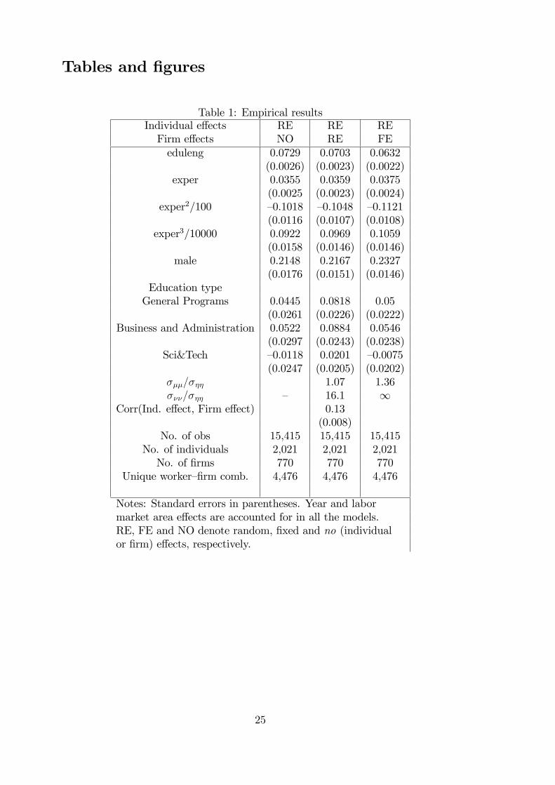
Empirical results Table 1 contains estimation results of the wage equation under

di¤erent assumptions with respect to the treatment of unobserved individual- and

�rm-speci�c heterogeneity.

[Table 1 here]

In the �rst speci�cation, column 1, an individual random e¤ects model is used

and no �rm controls are included; that is, these are the results for the RENO model.

The estimated return to an additional year of education is 0.073. This estimate seems

somewhat high. Turning to the models with �rm e¤ects outlined in Section 3, we

�nd that the returns to education become clearly smaller for the REFE speci�cation

(0.063), and less so for the RERE model (0.070). These �ndings may indicate that

models with random �rm e¤ects are misspeci�ed, being contaminated by omitted

variable bias. From Table 1 we notice that the parameter estimates obtained for

RENO and RERE are fairly equal. As mentioned in the introduction, this is to be

expected because they only di¤er in the parametrization of the covariance matrix of

the gross error terms. Furthermore, if we consider the RENO and the REFE esti-

mates together, we �nd that the latter is one percentage point smaller (13 percent)

than the former, a di¤erence that is quite substantial. An estimated di¤erence of

0.01 is also relatively large when we take statistical uncertainty into account (the

standard error is 0.002).

16

The parameter estimates for the experience coe¢ cients do not vary greatly be-

tween the three models. The maximum return to experience is found to be after

25�30 years of experience, and is more or less �at thereafter, as Figure A1 in the

appendix shows. The local minimum at about 45 years of experience is not a sub-

stantial feature, re�ecting the fact that only a few workers (less than 2.5 percent)

have such long experience. The estimates of the male dummy are greater than 0.20,

showing that the gender wage gap is signi�cant. This is quite large and should be

investigated further.11 None of the education-type parameters is found to be indi-

vidually statistically signi�cant for the RENO model. For the last two models in

which we control for unobserved �rm e¤ects, RERE and REFE, we �nd the dum-

mies for �General Programs�and �Business and Administration�to be statistically

signi�cant. These two groups include managers and administrative personnel.

The estimate of the correlation coe¢ cient between the unobserved individual

and �rm e¤ects in the RERE model is estimated as 0.13 and is highly signi�cant

(standard error< 0:01).12 This estimate is close to the 0.11 reported by Abowd et

al. (1999), who used a FEFE speci�cation. Torres et al. (2010) report a somewhat

higher positive estimate. On the other hand, Andrews et al. (2008), Grütter and

Lalive (2009) and Cornelißen and Hübler (2011) report negative estimates. How-

ever, the interpretation and comparison of these results in view of the substantial

question of sorting are not straightforward both because of the theoretical consid-

erations outlined by Eeckhout and Kircher (2010) and because our estimate relies

on a speci�cation whereby both unobserved individual and �rm heterogeneity are

represented by random e¤ects, whereas the above studies apply speci�cations in

which both components are assumed to be �xed e¤ects. The �xed e¤ects capture

11In this paper, we do not focus on gender di¤erences when modeling wages. We only considerthe male dummy as a control variable.12We also estimated a speci�cation of the RERE model in which we forced the correlation

between the �rm-speci�c and the individual-speci�c terms to be zero. This restriction leads toonly very small changes in the coe¢ cient estimates reported in Table 1, column (2).

17

the in�uence of all one-dimensional observed variables, whereas the random e¤ects

speci�cation only captures heterogeneity beyond what is already accounted for by

the inclusion of the time-invariant regressors.

Although our approach also covers the standard model with �xed individual-

speci�c e¤ects, FENO, and the FEFE model, these are of minor interest given that

we are interested in estimating the return to education, which is not identi�ed in

the presence of �xed individual e¤ects.13 Moreover, it is not possible to identify the

return to experience when we allow a general time trend (time dummies) because

(potential) experience increases linearly over time and therefore becomes collinear

with the time dummies and the dummies representing the �xed individual e¤ects.1415

We tested the RERE model against the REFE model (i.e., �xed �rm e¤ects)

using a Hausman test, in which the null hypothesis is that the RERE model is cor-

rect. The test statistic exceeded 95 (with 25 degrees of freedom), and the p-value

was practically equal to zero. Because Hausman tests routinely reject the random

e¤ect speci�cation in large samples, this test may not be very informative in our

case. The large estimated value of ���=��� compared with ���=���, reported in Ta-

ble 1 (i.e., 16:1 vs. 1:07), shows that �rm e¤ects have a more dispersed distribution

than do individual e¤ects. Note that in the limiting case when ���=��� tends to

in�nity, we obtain the REFE model. As mentioned above, neither the parameters

13For alternative algorithms of estimating the FEFE model, see Cornelissen (2008) andGuimarães and Portugal (2010).14We also ran the RENO model in which the stayers are added to the sample. In this way,

we found the estimate of the slope parameter of education length to be smaller, 0.0705, and theestimate of the parameter attached to the �rst-order power of experience to be 0.0415, that is,somewhat larger than the estimates reported in Table 1.15We performed a robustness check where we include mean number of employees per �rm in

the RENO model. This is in the spirit of Mundlak (1978). The estimation results obtained usingthis formulation are very similar to the results for the RENO and RERE speci�cations reported inTable 1. The estimate of the return to education is 0.0708, compared with 0.0729 in the RENOmodel and 0.0703 in the RERE model. One may think of the Mundlak approach as an alternativeto including �xed �rm e¤ects, but because the estimate of the return to schooling deviates fromthe estimate obtained using the REFE model, more time-invariant �rm-speci�c variables may beneeded to obtain better conformity.

18

corresponding to length of education nor those corresponding to experience are iden-

ti�ed in the model with �xed individual e¤ects; hence we cannot test REFE versus

FEFE (because they do not contain the same explanatory variables). In fact, the

time invariance of the education variable makes the use of individual-speci�c �xed

e¤ects models inappropriate. One alternative would have been to estimate the wage

equation using the estimator put forward by Hausman and Taylor (1981). However,

to use this approach it is necessary to identify which variables are correlated and

which are uncorrelated with the unobserved individual-speci�c e¤ect. In our case it

would be rather speculative to make such distinctions.

4 Concluding remarks

In this paper, we considered a general regression model with an unobserved random

e¤ect corresponding to the main observation unit and an unobserved e¤ect corre-

sponding to another type of unit with which the main observation unit is matched

at a given point in time. In an application, we examined di¤erent speci�cations of

real wage equations requiring access to employer�employee panel data. Such data

enable controls for both unobserved individual- and �rm-speci�c e¤ects. Earlier

contributions in this area� of those Abowd et al. (1999) being the best known

and most often cited� have stuck to a speci�cation with both �xed individual- and

�rm-speci�c e¤ects. However, a feature of such a speci�cation is that one cannot

identify e¤ects on the real wage of one-dimensional variables, such as length and

type of education or gender. Thus, it may be worthwhile to consider random e¤ects

speci�cations, as we have done in this paper. To estimate the model we applied the

Helmert transformation on the wage equation to sweep out the individual-speci�c

random e¤ects. To obtain estimates of the unknown parameters, the pro�le like-

lihood was maximized using the Expectation Conditional Maximization algorithm.

19

Using this approach, we �nd the estimate of return to education to become more

than 10 percent smaller when, in addition to controlling for unobserved individual

speci�c e¤ects, we control for �xed �rm-speci�c e¤ects.

20

References

[1] Abowd, J.M., Kramarz, F., and Margolis, D.N. (1999), �High Wage Workers

and High Wage Firms,�Econometrica, 67, 251�333.

[2] Abowd, J.M., Creecy, R.H., and Kramarz, F. (2002), �Computing Person and

Firm E¤ects Using Linked Longitudinal Employer�Employee Data (2002),�

Technical Paper 2002�2006. US Census Bureau.

[3] Andrews, M.J., Gill. L., Schank, T., and Upward, R. (2008), �High Wage Work-

ers and Low Wage Firms,�Journal of the Royal Statistical Society, Series A,

171, 673�697.

[4] Arellano, M., and Bover, O. (1995), �Another Look at the Instrumental Vari-

ables Estimation of Error Component Models,�Journal of Econometrics, 68,

29�51.

[5] Balestra, P., and Krishnakumar, J. (2008), �Fixed E¤ects Models and Fixed

Coe¢ cient Models,� in The Econometrics of Panel Data: Fundamentals and

Recent Developments in Theory and Practice, eds. Mátyás, L. and P. Sevestre,

Berlin: Springer, pp. 23�48.

[6] Blanchard, P., Gaigné, C., and Mathieu, C. (2008), �Foreign Direct Invest-

ments: Lessons from Panel Data,� in The Econometrics of Panel Data: Fun-

damentals and Recent Developments in Theory and Practice, eds. Mátyás, L.

and P. Sevestre, Berlin: Springer, pp. 663�696.

[7] Cornelissen, T. (2008), �The Stata Command felsdvreg to Fit a Linear Model

with Two High-Dimensional Fixed E¤ects,� Stata Journal, 8, 170�189.

[8] Cornelißen, T., and Hübler, O. (2011), �Unobserved Individual and Firm Het-

21

erogeneity inWage and Job Duration Functions: Evidence from German Linked

Employer�Employee Data,�German Economic Review (forthcoming).

[9] Demidenko, E. (2004), Mixed Models: Theory and Applications, Hoboken, New

Jersey: Wiley.

[10] Dempster, A.P., Laird. N.M., and Rubin, D.B. (1977), �Maximum Likelihood

from Incomplete Data via the EM Algorithm (with discussion),�Journal of the

Royal Statistical Society, Series B, 39, 1�38.

[11] Eeckhout, J., and Kircher, P. (2010), �Identifying Sorting �In Theory,�LSE

Research Online.

[12] Francke, M.K., Koopman, S.J., and De Vos, A.F. (2010), �Likelihood Functions

for State Space Models with Di¤use Initial Conditions,�Journal of Time Series

Analysis, 31, 407�414.

[13] Godager, G., and Biørn, E. (2010), �Does Quality In�uence Choice of General

Practitioner? An Analysis of Matched Doctor�Patient Panel Data,�Economic

Modelling, 27, 842�853.

[14] Goux, M., and Maurin, E. (1999), �Persistence of Interindustry Wage Di¤er-

entials Using Matched Worker-Firm Data,� Journal of Labor Economics, 17,

492�533.

[15] Grütter, M., and Lalive, R. (2009), �The Importance of Firms in Wage Deter-

mination,� Labour Economics, 16, 149�160.

[16] Guimarães, P., and Portugal, P. (2010), �A Simple Feasible Procedure to Fit

Models with High-Dimensional Fixed E¤ects,� Stata Journal, 10, 628�649.

22

[17] Hausman, J.A., and Taylor, W.E. (1981), �Panel Data and Unobservable Indi-

vidual E¤ects,� Econometrica, 49, 1377�1398.

[18] Heyman, F. (2007), �Firm Size or Firm Age? The E¤ects on Wages Using

Matched Employer�Employee Data,�Labour, 21, 237�263.

[19] Ioannidou, V., and Ongena, S. (2010), ��Time for a Change�: Loan Conditions

and Bank Behavior when Firms Switch Banks,�Journal of Finance, 65, 1847�

1877.

[20] Keane, M.P., and Runkle, D.E. (1992), �On the Estimation of Panel-Data

Models when Instruments are not Strictly Exogenous,� Journal of Business

and Economic Statistics, 10, 1�9.

[21] Lallemand, T., Plasman, R., and Rycx, F. (2005), �Why Do Large Firms Pay

Higher Wages? Evidence from Matched Worker�Firm Data,� International

Journal of Manpower, 26, 705�723.

[22] Meng, X.-L., and Rubin, D.B. (1993), �Maximum Likelihood Estimation via

the ECM Algorithm: A General Framework,� Biometrika, 80, 267�278.

[23] Mundlak, Y. (1978), �On the Pooling of Time Series and Cross Section Data,�

Econometrica, 46, 69�85.

[24] Plasman, R., Rycx, F., and Tojerow, I. (2007), �Wage Di¤erentials in Belgium:

The Role of Worker and Employer Characteristics,� Cahiers Economiques de

Bruxelles, 50, 11�40.

[25] Searle, S.R., Casella, G., and McCulloch, C.E. (1992), Variance Components,

New York: Wiley.

23

[26] Torres, R., Portugal, P., Addison, J.T., and Guimarães, P. (2010), �The Sources

of Wage Variation: An Analysis Using Matched Employer Employee Data,�

Working Papers 25/2010, Banco de Portugal.

24

Tables and �gures

Table 1: Empirical resultsIndividual e¤ects RE RE REFirm e¤ects NO RE FEeduleng 0.0729 0.0703 0.0632

(0.0026) (0.0023) (0.0022)exper 0.0355 0.0359 0.0375

(0.0025 (0.0023) (0.0024)exper2/100 �0.1018 �0.1048 �0.1121

(0.0116 (0.0107) (0.0108)exper3/10000 0.0922 0.0969 0.1059

(0.0158 (0.0146) (0.0146)male 0.2148 0.2167 0.2327

(0.0176 (0.0151) (0.0146)Education typeGeneral Programs 0.0445 0.0818 0.05

(0.0261 (0.0226) (0.0222)Business and Administration 0.0522 0.0884 0.0546

(0.0297 (0.0243) (0.0238)Sci&Tech �0.0118 0.0201 �0.0075

(0.0247 (0.0205) (0.0202)���=��� 1.07 1.36���=��� � 16.1 1

Corr(Ind. e¤ect, Firm e¤ect) 0.13(0.008)

No. of obs 15,415 15,415 15,415No. of individuals 2,021 2,021 2,021No. of �rms 770 770 770

Unique worker��rm comb. 4,476 4,476 4,476

Notes: Standard errors in parentheses. Year and labormarket area e¤ects are accounted for in all the models.RE, FE and NO denote random, �xed and no (individualor �rm) e¤ects, respectively.

25

Appendix

Table A1: The unbalancedness of the panel dataNumber of years Number of persons Number of observations

a person is in the sample in the sample2 87 1743 153 4594 203 8125 184 9206 168 1,0087 165 1,1558 173 1,3849 180 1,62010 171 1,71011 271 2,98112 266 3,192Sum 2,021 15,415

Table A2. Overview of number of �rms in workers�employment historyNumber of �rms Number of individuals having worked in the indicated number of �rms2 1,6503 3124 555 4Total 2,021

26

RENOREFE

RERE

0 5 10 15 20 25 30 35 40 45 50

0.05

0.10

0.15

0.20

0.25

0.30

0.35

0.40

exper

RENOREFE

RERE

Figure A.1: The partial e¤ect of experience on expected log-wage. Estimates for threemodel speci�cations.

27