Discussion Papers in Economics

Department of Economics University of Surrey

Guildford Surrey GU2 7XH, UK

Telephone +44 (0)1483 689380 Facsimile +44 (0)1483 689548 Web www.econ.surrey.ac.uk

ISSN: 1749-5075

EFFICIENT SIMULATION OF DSGE MODELS WITH

INEQUALITY CONSTRAINTS

By

Tom Holden (University of Surrey)

&

Michael Paetz (University of Hamburg)

DP 16/12

01/10/2012

Page 1 of 20

Efficient   simulation   of   DSGE   models   with  inequality  constraints

Tom Holden1, School of Economics, University of Surrey

Michael Paetz2, Univeristy of Hamburg, Department of Economics

Abstract: This paper presents a fast, simple and intuitive algorithm for simulation of linear dynamic

stochastic general equilibrium models with inequality constraints. The algorithm handles both the

computation of impulse responses, and stochastic simulation, and can deal with arbitrarily many

bounded variables. Furthermore, the algorithm is able to capture the precautionary motive

associated with the risk of hitting such a bound. To illustrate the usefulness and efficiency of this

algorithm we provide a variety of applications including to models incorporating a zero lower bound

(ZLB) on nominal interest rates. Our procedure is much faster than comparable methods and can

readily handle large models. We therefore expect this algorithm to be useful in a wide variety of

applications.

Keywords: Inequality constraints, Zero lower bound, Precautionary motives, Two-country models

JEL Classification: C63, E32, E43, E52

1 Contact address: School of Economics, FBEL, University of Surrey, Guildford, GU2 7XH, England Contact email: thomas.holden@gmail.com Web-site: http://www.tholden.org/ 2 Contact address: Fakultät für Wirtschafts- und Sozialwissenschaften, Universität Hamburg, Von-Melle-Park 9, 20146 Hamburg, Deutschland Contact email: michael.paetz@wiso.uni-hamburg.de The authors would like to acknowledge helpful comments on earlier drafts of the paper from Michael Funke, William T. Gavin, Matteo Iacoviello, Michel Juillard, Paul Levine, Jesper Lindé, Antonio Mele, Søren Ravn and Simon Wren-Lewis, along with those from other participants in the 8th Dynare Conference.

01/10/2012

Page 2 of 20

1. Introduction New Keynesian (NK) Dynamic Stochastic General Equilibrium (DSGE) models are today's standard framework for analysing central bank policies.3 The nominal and real rigidities in these models mean central banks may improve welfare through monetary policy. Traditionally, DSGE models are log-linearised, which results in both computational and analytic tractability. However, the simplicity of this approach also neglects important non-linearities, not-least inequality constraints, of which the zero lower bound (ZLB) on interest rates is the most prominent example. In this paper, we present an efficient algorithm for simulating DSGE models subject to arbitrarily many inequality constraints, at arbitrary accuracy, at least away from the bound.

Macroeconomic analysis had ignored the zero lower bound almost completely before the experience of Japan in the 1990s, since the bulk of macroeconomists believed the constraint would bind only for a short time span (if at all). Under this presumption, the effects would be negligible, and so ignoring the bound seemed to be a reasonable simplification. However, the interest rates in Japan during the 1990s, as well as those in the US over the last few years, disabused researchers and policymakers of this popular fallacy.

In the aftermath of the crisis, the transmission of monetary policy under the ZLB became an important matter for central banks and academia. To cope with the bound, researchers either solve such non-linear models using global approximation methods (which come at a dramatic increase in computational costs, and scale exceptionally poorly) or use deterministic setups. This paper provides a fast, simple and intuitive algorithm to deal with inequality constraints in perturbation approximations to DSGE models, which correctly captures the precautionary motives associated with such bounds. The code is designed to work with Dynare (Adjemian et al. 2011), so incorporating it into existing models is trivial. The method is not only useful for deriving impulse response functions (IRFs), but can also be used for stochastic simulations, opening up the possibility of particle filter based estimation of models with inequality constraints. The method endogenously determines when the constraint will bind, and can handle constraints that may bind in multiple disjoint runs, or that may not begin to bind until long after the initial impulse. The general idea is to introduce “shadow price shocks”, which hit the bounded variables every time the constraint is violated, and “push” these variables back to zero. To ensure the solution is consistent with rational expectations, these shocks are expected by agents in advance, so they may be thought of as a kind of endogenous news shock.

This algorithm is not solely useful for modelling a ZLB on interest rates, but can be used for any model including constrained variables. Holden (2010), for example, uses it to constrain invention rates to be positive in a model of endogenous growth. In addition, Funke and Paetz (2012) use this technique to evaluate threshold loan-to-value policies in Hong Kong, where policymakers decrease the loan-to-value ratio, when property price inflation exceeds a certain value. In Chen et al. (2012), the same method   is   used   to  model   the   People’s   Bank   of   China’s interest rate corridor on retail lending and deposit rates.

3 See Clarida et al. (1999) for an early literature review on NK models.

01/10/2012

Page 3 of 20

The rest of the paper is organized as follows. In section 2, the algorithm is described and related to the existing literature. Section 3 assesses the accuracy of the procedure in a variety of models for which high accuracy solutions are available, and section 4 goes on to provide some sample applications to larger models. The final section concludes.

2. The numerical method

2.1. The existing literature

Due to the recent experience of the US and Europe, the literature on (stochastic) simulation of models with a ZLB has grown rapidly in the past few years. The most important contributions include Eggertsson and Woodford (2003), Erceg and Lindé (2010), Braun and Körber (2011), Christiano et al. (2011) and Fernández-Villaverde et al. (2012). In what follows, we highlight the similarities and differences between the approaches employed in these papers and the method presented in this paper.4

The first generation of papers used variants of the method proposed by Eggertsson and Woodford (2003), in an appendix. This relied on a piecewise linear approximation to the model, with the model being driven by a two-state Markov chain with an absorbing state. Once the ZLB is hit, there is a positive probability in each period that the discount factor jumps to its long run value, at which point the ZLB will never be hit again. Obviously, this is a highly restrictive assumption. A version of this algorithm without the restriction has been proposed by Jung et al. (2005), and implemented in full generality in Dynare by Guerrieri and Iacoviello (2012). Nonetheless, the algorithm still relies on a linear approximation, which the results of Braun et al. (2012) suggest may lead to unreliable conclusions in the presence of the ZLB.

The next generation of papers used nonlinear perfect foresight solvers. These include Coenen et al. (2004), Braun and Körber (2011) and  the  “extended  path”  method  of  Adjemian  and  Juillard  (2011). These solve the  model’s  nonlinear  equations, under the assumption that eventually (e.g. after 100 periods) the model is guaranteed to have returned to steady state. Such methods fully capture the nonlinearities of the model, but because they solve under perfect foresight, they omit any “precautionary  motives”   including   those   that   arise   from   the   risk  of  hitting   the   ZLB.   Furthermore,  since the model has to have returned to steady state up to machine precision by the final period considered, they require a very large number of nonlinear equations to be solved. This means they tend to both be prohibitively slow, and unstable, with the algorithm frequently failing to find a solution to the equations.

A third strand of the literature considers global approximations to models containing inequality constraints, with Fernández-Villaverde et al. (2012) doing this for a small scale NK model, using the Smolyak collocation method of Krueger et al. (2011). Global methods successfully capture both the model’s   nonlinearities   and   precautionary   motives;   however,   they   are   subject   to   a   curse   of  

4 See the introduction in Braun et al. (2012) for a survey on models including a zero lower bound. An early analysis of the zero lower bound in a deterministic model can also be found in Fuhrer and Madigan (1997).

01/10/2012

Page 4 of 20

dimensionality that renders them infeasible in the medium scale NK models we usually consider. While global methods that avoid the curse of dimensionality have been developed by Maliar et al. (2011), these rely on an  endogenous  grid  constructed  from  the  model’s  ergodic  set,  which  is  likely  to lead to low accuracy at the ZLB if this bound is only hit occasionally.

Our method represents a compromise between the accuracy of global methods, and the speed and scalability of linear ones, much like standard high order perturbation approximations. The paper that is probably most closely related to our work is Erceg and Lindé (2010), which we were not aware of until after the completion of the first version of our algorithm in Holden (2010). The authors rely on techniques, explained in an unpublished mimeo of James Hebden, Jesper Lindé and Lars Svensson, which, like our algorithm, are based on the idea of adding shocks to the bounded variable. Since we have not seen this mimeo, we are unable to relate our work to this algorithm, but we are confident that our method is novel in several respects. Firstly, it is designed to take advantage of existing algorithms both for simulating DSGE models (e.g. those of Dynare), and algorithms for quadratic programming, leading to its high speed. Secondly, it is generalized to permit any number of constrained variables. Thirdly, it is extended for use in stochastic simulations, permitting us to derive average IRFs, and opening up the possibility of estimating bounded models. Finally, it is generalized to perturbation approximations of arbitrary order, which is what enables the algorithm to capture precautionary incentives, thus improving on the accuracy of nonlinear perfect foresight algorithms.

2.2. Our basic IRF algorithm with a single bound

Suppose we have a rational expectations model in the variables 𝑥 , , … , 𝑥 , , and we are interested in the response to the shock, 𝜖 .  Initially,  we  will  suppose  further  that  all  of  the  model’s  equations  are linear, except one that takes the form:

𝑥 , = max{0, 𝜇 + 𝜙 𝑥 + 𝜙 𝑥 + 𝜙 𝔼 𝑥 − (𝜙 + 𝜙 + 𝜙 )𝜇}, (2.1)

where 𝑥 is the vector 𝑥 , , 𝑥 , , … , 𝑥 , , 𝜇 = 𝜇 , 𝜇 , … , 𝜇 is  a  vector  stacking  the  variables’  steady state values and 𝜇 > 0. We can transform any linear model with a bound into this form through the addition of appropriate auxiliary variables.5

Now, a shock that drives 𝑥 , to 0 for some number of periods is like a combination of the original shock, and a news shock stating 𝑥 , will be higher than expected for some duration. We call these news   shocks   “shadow   price   shocks”   as   in   a   model   with   bounded   assets,   they   represent the Lagrange multiplier on the constraint. The key to the simplicity of our algorithm is the fact that in

5 So, if the bounded equation stated that 𝑥 = max{𝑥 , 𝑦 } (where ~ denotes unconstrained variables), with 𝑥 > 𝑦 in steady state, we would add an auxiliary variable defined as 𝑥 − 𝑦 , noting that 𝑥 = 𝑦 + max{0, 𝑥 − 𝑦 }. The models of Funke and Paetz (2012) and Chen et al. (2012) include variables that are bounded at a positive value, for example. When 𝑥 = 𝑦 in steady state, we instead add the variable 𝑦 − 𝑥 , and note that 𝑥 = 𝑥 +max{0, 𝑦 − 𝑥 }. If the model is in levels, rather than in logs, it may be preferable to define auxiliary variables as ratios rather than differences. In this case, rather than adding shadow shocks, we must multiply by their exponentials.

01/10/2012

Page 5 of 20

linear models, the IRF to a linear combination of shocks is equal to the same linear combination of

each  shock’s  IRF.6

Let us start by defining 𝑣 to be the column vector containing the relative impulse response of

variable 𝑥 to the shock, ignoring the ZLB. Let 𝑇∗ be the number of periods after which the

constraint is no longer expected to bind. Note that this will in general be much smaller than the

time it takes to return to steady state. We assume that the IRF vectors are of length 𝑇, where

𝑇 ≥ 𝑇∗.

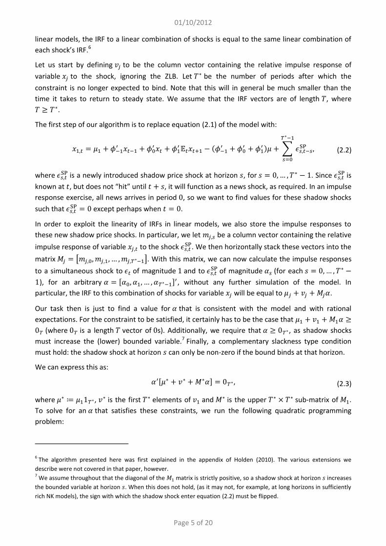
The first step of our algorithm is to replace equation (2.1) of the model with:

𝑥 , = 𝜇 + 𝜙 𝑥 + 𝜙 𝑥 + 𝜙 𝔼 𝑥 − (𝜙 + 𝜙 + 𝜙 )𝜇 + 𝜖 ,

∗

, (2.2)

where 𝜖 , is a newly introduced shadow price shock at horizon 𝑠, for 𝑠 = 0,… , 𝑇∗ − 1. Since 𝜖 , is

known at 𝑡,  but  does  not  “hit”  until  𝑡 + 𝑠, it will function as a news shock, as required. In an impulse

response exercise, all news arrives in period 0, so we want to find values for these shadow shocks

such that 𝜖 , = 0 except perhaps when 𝑡 = 0.

In order to exploit the linearity of IRFs in linear models, we also store the impulse responses to

these new shadow price shocks. In particular, we let 𝑚 , be a column vector containing the relative

impulse response of variable 𝑥 , to the shock 𝜖 , . We then horizontally stack these vectors into the

matrix 𝑀 = 𝑚 , ,𝑚 , , … ,𝑚 , ∗ . With this matrix, we can now calculate the impulse responses

to a simultaneous shock to 𝜖 of magnitude 1 and to 𝜖 , of magnitude 𝛼 (for each 𝑠 = 0,… , 𝑇∗ −1), for an arbitrary 𝛼 = [𝛼 , 𝛼 , … , 𝛼 ∗ ] , without any further simulation of the model. In

particular, the IRF to this combination of shocks for variable 𝑥 will be equal to 𝜇 + 𝑣 +𝑀 𝛼.

Our task then is just to find a value for 𝛼 that is consistent with the model and with rational

expectations. For the constraint to be satisfied, it certainly has to be the case that 𝜇 + 𝑣 +𝑀 𝛼 ≥0 (where 0 is a length 𝑇 vector of 0s). Additionally, we require that 𝛼 ≥ 0 ∗, as shadow shocks

must increase the (lower) bounded variable.7 Finally, a complementary slackness type condition

must hold: the shadow shock at horizon 𝑠 can only be non-zero if the bound binds at that horizon.

We can express this as:

𝛼 [𝜇∗ + 𝑣∗ + 𝑀∗𝛼] = 0 ∗, (2.3)

where 𝜇∗ ≔ 𝜇 1 ∗, 𝑣∗ is the first 𝑇∗ elements of 𝑣 and 𝑀∗ is the upper 𝑇∗ × 𝑇∗ sub-matrix of 𝑀 .

To solve for an 𝛼 that satisfies these constraints, we run the following quadratic programming

problem:

6 The algorithm presented here was first explained in the appendix of Holden (2010). The various extensions we

describe were not covered in that paper, however. 7 We assume throughout that the diagonal of the 𝑀 matrix is strictly positive, so a shadow shock at horizon 𝑠 increases

the bounded variable at horizon 𝑠. When this does not hold, (as it may not, for example, at long horizons in sufficiently

rich NK models), the sign with which the shadow shock enter equation (2.2) must be flipped.

01/10/2012

Page 6 of 20

𝛼∗ ≔ arg  min

∗∗ ∗ ∗ ∗

𝛼 (𝜇∗ + 𝑣∗) +12𝛼 (𝑀∗ + 𝑀∗ )𝛼 ,

(2.4)

where the solution is considered admissible if the minimand is 0 at the optimum (i.e. equation (2.3)

is satisfied).8 Since there are well-established, fast, robust algorithms for quadratic programming,

this is then a straightforward problem.9

The standard properties of quadratic programming problems imply that a sufficient condition for

the existence of a unique solution to (2.4) is that 𝑀∗ +𝑀∗ is positive definite. In our experience,

this is satisfied in only the simplest models. When 𝑀∗ +𝑀∗ is not positive definite, we cannot rule

out the existence of multiple solutions. In these cases, which solution is returned will depend on the

precise properties of the quadratic programming algorithm used. However, for most models the

construction of our problem will lead the algorithm to select the solution in which the components

of 𝛼 are as small as possible, which will also tend to minimise the amount of time the constraint

binds. If desired, explicit guarantees on the solution selected may be enforced via homotopy

methods,10 though this will increase the time cost of our algorithm.

It is also possible that there will be no admissible solution to (2.4), at least for sufficiently large

shocks. This   will   happen   if   there   are   “complementarities”   between   constraints:   e.g.   hitting   one  constraint increases the chance of hitting another constraint and vice versa. Obviously, this is much

more likely when there are multiple bounds, rather than merely multiple horizons. A necessary

condition for the existence of an admissible solution to (2.4) for arbitrarily large shocks is that there

exists some 𝛼 ≥ 0 ∗ such that 𝑀∗𝛼 ≥ 1 ∗. In simple models the anticipation effects of hitting the

bound in future are weak, so this condition will be satisfied, but in medium scale models, we will

generally not be able to provide such a guarantee.

2.3. Dealing with multiple bounds

The algorithm previously described may be readily generalised to cases with multiple bounds.

Suppose that in the set-up above, rather than just 𝑥 , being bounded, each of the variables

𝑥 , , 𝑥 , , … , 𝑥 ∗, is bounded, with a corresponding equation taking the form of (2.1). Much as

before, we add shadow shocks to each of these equations (giving a total of 𝑛∗𝑇∗ extra shocks), and

we horizontally concatenate the impulse responses of variable 𝑥 , to each of the shadow shocks in

the equation for 𝑥 , into the matrix 𝑀 , . We then define 𝑀 ,∗ to be the upper 𝑇∗ × 𝑇∗ sub-matrix of

𝑀 , , and 𝑀∗ to be the 𝑛∗𝑇∗ × 𝑛∗𝑇∗ block-matrix with (𝑗, 𝑙)th block 𝑀 ,∗ for 𝑗, 𝑙 ∈ {1, … , 𝑛∗}. Likewise,

we define 𝜇∗ ≔ 𝜇 1 ∗, 𝑣∗ to be the first 𝑇∗ elements of 𝑣 , and 𝜇∗ and 𝑣∗ to be the length 𝑛∗𝑇∗

block vectors with 𝑙th block 𝜇∗ and 𝑣∗, respectively. With these (re-)definitions, an admissible

8 The constraint 𝜇∗ + 𝑣∗ + 𝑀∗𝛼 ≥ 0 ∗ may also be replaced with 𝜇 + 𝑣 + 𝑀 𝛼 ≥ 0 to check there are no bound

violations after 𝑇∗. 9 In  MATLAB,  these  are  provided  by  the  “quadprog”  command.

10 To guarantee selecting the equilibrium in which ‖𝛼‖ is minimal, we replace 𝑀∗ + 𝑀∗ by 𝑀∗ +𝑀∗ + 𝜆𝐼, where

𝜆 → 0 is the homotopy parameter. To guarantee selecting the equilibrium in which ‖𝛼‖ is minimal, we replace 𝜇∗ + 𝑣∗

by 𝜇∗ + 𝑣∗ + 𝜆1 ∗, where 𝜆 → 0 is the homotopy parameter.

01/10/2012

Page 7 of 20

solution to (2.4) again gives us the required combination of shadow shocks to enforce all bounds, and the uniqueness and existence conditions are identical as well.

2.4. Stochastic simulation

The algorithm of the previous sections may be readily extended to the stochastic simulation of bounded, linear models.11 As before we begin by adding shadow price shocks to the equations defining bounded variables. Now suppose we have simulated up to period 𝑡 − 1. In a linear model, agents’ expectations at 𝑡 of the state of the economy at 𝑡 + 1, 𝑡 + 2,… are the same as they would be were the variance of all shocks equal to 0 from 𝑡 + 1 onwards. This will not be exactly true in a model with bounds, since the bounds will tend to increase the means of lower bounded variables. However, since (log-)linearisation has already removed any effects of uncertainty on the mean, if we solve assuming there are no shocks after period 𝑡, our approximation error is likely to be of the same order as that of a (log-)linearised model without constraints,12 at least providing the precautionary incentives stemming from the risk of hitting the bound are fairly weak.

Thus, much as in the IRF case, we first simulate the model to find the path by which it would return to the steady-state, in the absence of bounds, and with no shocks arriving after period 𝑡. If the constraints are not violated along this path, then our simulated value for period 𝑡 is fine, and we may move on to period 𝑡 + 1. Otherwise, shadow shocks must be added. The algorithm for doing this is identical to that described above for IRFs, except that the simulated return paths of the economy’s variables take the role of 𝜇∗ + 𝑣∗ above. (We again use the 𝑀 ,

∗ matrices formed from the impulse responses to shadow shocks.) The found solution to the quadratic programming problem gives a valid, new value for variables at 𝑡, enabling us to go on to the next period. Note that it is now  no  longer  the  case  that  the  “news” contained in shadow shocks is guaranteed to come true, since other shocks may arrive in the meantime pushing us away from the bounds. Consequently, 𝛼 no  longer  represents  the  found  value  of  today’s  shadow  price  shock.  Rather,  it  is  equal to the cumulated history of shadow price shocks that hit in period 0 (i.e. 𝜖 , + 𝜖 , + ⋯+𝜖 ∗ , ∗ ).

2.5. Average IRFs

Using our simulation algorithm we can go on to produce average IRFs, i.e. IRFs that give a measure of the average response of the model to a one standard deviation shock, rather than a measure of the response in steady-state. (The two measures agree in the absence of bounds.) To do this, we run a stochastic simulation of the model, and then rerun the same simulation with the same shocks in all periods except one, in which we add 1 to the shock of interest. The difference between these two simulations gives one sample IRF, and the average of many such sample IRFs gives us our average IRF.13

11 The algorithm described here was first publicly described by Tom Holden at http://bit.ly/I0nAHf. 12 An identical approximation is made in the non-linear case by Adjemian and Juillard (2011). 13 This is the algorithm used by Dynare for constructing IRFs in non-linear models. See http://www.dynare.org/DynareWiki/IrFs.

01/10/2012

Page 8 of 20

2.6. Estimating Bounded Models

Our method for simulating models incorporating a zero lower bound naturally leads to an algorithm for particle filter based estimation of them. Indeed, since the observation equations are still linear in the state, and the transition equations are near linear, this is likely to be far more efficient than particle filter estimation of second order approximations to standard DSGE models (as in Fernández-Villaverde and Rubio-Ramírez (2010)). Indeed, since our solution method readily delivers last  period’s  expectation  of  today’s shadow price shock, we can write down a close approximation to the model for which the transition  equations  are  linear  in  today’s shock. For this approximated model, the optimal particle filter “proposal distribution” may be derived analytically, giving us a near optimal proposal distribution for the actual model, and enabling us to get high accuracy out of a small number of particles. We intend to assess the practical performance of this method in future work.

2.7. Generalisation to approximations of arbitrary order

The recent work of Braun et al. (2012) brought to light some serious problems with log-linearised solutions to models with a ZLB. They illustrate that the log-linearised equilibrium conditions can be misleading with respect to the existence and uniqueness of equilibrium, and may lead  to  “wrong”  dynamics under the ZLB. For example, they show that in a simple NK model with Rotemberg (1996) quadratic  price  adjustment  cost,  the  “paradox  of  toil”14 disappears in the fully nonlinear model, at least when solved under perfect foresight. The authors pinpoint the resource cost of price adjustment, which is zero in a linearised model, as being the key to this discrepancy. The paper shows that these costs work as automatic stabilizers that reduce the variation in marginal costs and inflation, and decrease the government spending multiplier at the ZLB.

In fact, even fully nonlinear perfect foresight solutions may be misleading at the ZLB. For example, Adjemian and Juillard (2011) evaluate the accuracy of the (fully non-linear perfect foresight) extended path approach in a small-scale DSGE model and show that the accuracy drops significantly when the ZLB is hit regularly. Furthermore, using global methods, Fernández-Villaverde et al. (2012) find that when the interest rate stays at the ZLB for a prolonged time period, the government spending multiplier does indeed become large, contrary to the claims of Braun et al. (2012), again suggesting that the assumption of perfect foresight may itself be a source of substantial inaccuracy in the presence of a ZLB. Our algorithm provides an answer to these worries, as it may be readily generalised  to  “pruned” perturbation approximations (Sunghyun Henry Kim et al. 2008) of arbitrary order, and these approximations may be so constructed as to capture the precautionary motive arising from the risk of hitting the ZLB in future.

The key to ensuring our algorithm works at higher orders, is that in a 𝑑th order pruned perturbation approximation, shocks of the form 𝜖 only enter linearly,15 hence, if we use shocks of the form

𝜖 , as shadow shocks, then our algorithm will work much as before, with the expected path implied by the pruned perturbation approximation taking the place of the expected path under

14 A fall in employment after a labour tax cut at the ZLB. See Eggertsson and Woodford (2003). 15 See equation (36) of (Sunghyun Henry Kim et al. 2008).

01/10/2012

Page 9 of 20

perfect foresight. Using shocks of the highest available order as shadow shocks is also consistent with perturbation approximation theory, since with Gaussian shocks the probability of hitting the ZLB is 𝜊(𝜎 ) for any 𝑑 ∈ ℕ, where 𝜎 is the perturbation parameter controlling the variance of shocks.

To capture the precautionary motive arising from the risk of hitting the ZLB in future we require 𝑑

to be even, since in that case 𝜖 , is positive in expectation.16 This enables us to capture the effects   of   the   ZLB   on   each   series’ mean, removing the deficiency in our stochastic simulation algorithm previously noted. To do this requires us to first solve a fixed-point problem to ensure that the variance of 𝜖 , used in constructing the perturbation approximation actually agrees with the variance that is implied by the simulated mean values of 𝛼. In practice, the fixed-point problem is solved by standard numerical optimisation algorithms, at low accuracies since each residual evaluation requires the computation of simulated moments. We also found it helpful to treat the non-stochastic steady-state inflation target as an additional parameter to be optimised, to hold the mean level of inflation constant.

It is also possible to approximate around the risky steady state, following Juillard (2011), within our algorithm.   This   enables   the  model’s   responses   to   reflect   better   the   differences   in   all   equations’  slope close to the ZLB.

At sufficiently high (even) orders of perturbation approximation, our algorithm (using either the non-stochastic steady state or the risky steady state) must beat any perfect foresight method in terms of accuracy, since it captures the effects of uncertainty  on  the  variables’ means. Indeed, we show in the next section that even at order 2 our algorithm beats the extended path in standard models. Our algorithm is likely to be particularly   useful   for   the   analysis   of   “paradox of toil”-type effects, since it enables the analysis of the effects of the ZLB even in second order approximations to large models.

3. Accuracy

3.1. A borrowing constraints model

We begin with a very simple model taken from Guerrieri and Iacoviello (2012).

An  individual’s  income  follows  the  process  log 𝑌 = 𝜌 log 𝑌 + 𝜎 1 − 𝜌 𝜀 , where 𝜀 ~NIID(0,1), 𝜎 = 0.03 and 𝜌 = 0.9. This income may be used for consumption 𝐶 or saving, and it also acts as collateral. There is a collateral constrain on total borrowing, 𝐵 , that states that 𝐵 ≤ 𝑀𝑌 , with 𝑀 = 2. Consumers maximise the utility function:

𝑈 = 𝔼 𝛽 log 𝐶 ,

16 Our algorithm will not always generate positive values for 𝜖 , as news may not be realised. However, since 𝜖 , only enters into the transition equations when raised to the power of 𝑑, this will not result in complex numbers entering into the simulated paths.

01/10/2012

Page 10 of 20

with 𝛽 = 0.94, subject to the collateral constraint and subject to the budget constraint 𝐶 = 𝑌 +𝐵 − 𝑅𝐵 , with 𝑅 = 1.05. In normal times, the collateral constraint binds, so in place of the standard Euler equation we use the equations:

𝐴 = max 0,1

(1 + 𝑀)𝑌 − 𝑅𝐵− 𝔼

𝛽𝑅𝐶

1𝐶

= 𝔼𝛽𝑅𝐶

+ 𝐴

where 𝐴 is an auxiliary variable.

Pr𝐵𝑌

> 1.98 𝔼 log𝐶 Var log𝐶 Corr(log 𝐶 , log𝑌 ) Linear17 100% −0.1054 0.0480 0.75 Log-linear18 100% −0.1043 0.0475 0.77 Piecewise linear17 88% −0.1051 0.0426 0.82 Extended path 89% −𝟎.𝟏𝟎𝟒𝟓 0.0431 0.84 Our algorithm order 118 88% −0.1040 0.0427 0.85 Our algorithm order 218 𝟖𝟓% −0.1046 𝟎. 𝟎𝟒𝟐𝟎 𝟎. 𝟖𝟔 Value function17 79% −0.1045 0.0403 0.86

Table 1: An accuracy comparison in the simple borrowing constraints model of Guerrieri and Iacoviello (2012).

In Table 1 below we present a comparison of the results of our algorithms with the piecewise linear algorithm of Guerrieri and Iacoviello (2012) and the extended path method of Adjemian and Juillard (2011). All values except those taken from Guerrieri and Iacoviello (2012) were generated from a run of 10000 periods. The shaded cells with bold text show the results coming closest to the value function iteration results, and the shaded cells without bold text show the next closest values. Our second order algorithm comes closest to the value function iteration results along three out of the four metrics considered, and is a runner up in that fourth case. Indeed, for this model, even our first order algorithm beats the extended path algorithm in three cases out of four. However, it is only really the second order version that can come close to matching the percentage of time in which the constraint binds, by virtue of taking into account the incentive to save to avoid it.

3.2. An NK model

We now turn to the NK model of Fernández-Villaverde et al. (2012). This is a standard nonlinear NK model with sticky prices, labour choice, flexible wages, Taylor rule monetary policy and a stochastic share of government spending in output. The equilibrium conditions for this model are given in the first appendix, section 7.1, and we calibrate to the same standard values as Fernández-Villaverde et al. (2012).

To assess our accuracy, we treat the solution of Fernández-Villaverde et al. (2012) as  the  “truth”,  and measure the deviations between their simulated paths19 and the paths generated by our

17 Taken from Guerrieri and Iacoviello (2012). 18 With 𝑌 and 𝐶 simulated in logs. 19 We would like to thank Grey Gordon for providing us with this data.

01/10/2012

Page 11 of 20

algorithms (with all variables in logs) and the extended path method of Adjemian and Juillard (2011). All paths were length 30000 periods. We report the norms of these errors for consumption, nominal interest rates and inflation in Tables 2, 3 and 4 respectively. (Cells are formatted as before.)

1 norm 2 norm ∞ norm Log-linear 364.0 1.011 0.03816 Extended path 311.0 0.7575 0.01792 Our algorithm order 1 336.7 0.8120 0.03593 Our algorithm order 2 𝟐𝟕𝟔. 𝟏 𝟎. 𝟔𝟗𝟐𝟒 𝟎. 𝟎𝟏𝟕𝟖𝟎

Table 2: Norms of the approximation errors in log consumption in the NK model of Fernández-Villaverde et al. (2012).

1 norm 2 norm ∞ norm Capped log-linear20 314.4 0.8344 0.01096 Extended path 𝟑𝟏𝟏. 𝟔 0.8240 0.01064 Our algorithm order 1 314.4 0.8344 0.01096 Our algorithm order 2 313.8 𝟎. 𝟖𝟏𝟒𝟒 𝟎. 𝟎𝟏𝟎𝟓𝟎

Table 3: Norms of the approximation errors in log gross nominal interest rates in the NK model of Fernández-Villaverde et al. (2012).

1 norm 2 norm ∞ norm Log-linear 217.7 0.6021 0.01576 Extended path 𝟐𝟎𝟔. 𝟓 𝟎. 𝟓𝟓𝟓𝟓 0.01387 Our algorithm order 1 212.8 0.5695 0.01381 Our algorithm order 2 208.2 0.5621 𝟎. 𝟎𝟎𝟗𝟐𝟎𝟑

Table 4: Norms of the approximation errors in log inflation in the NK model of Fernández-Villaverde et al. (2012).

At second order, our algorithm beats the extended path algorithm for consumption whichever norm is used. This is unsurprising since consumption is sensitive to risk. For the nominal interest rate, it beats the extended path method with respect to the 2 norm or the ∞ norm, but not with respect to the 1 norm. This implies the extended path algorithm is capable of closely following interest rates a lot of the time, but occasionally it is a long way off, perhaps because of its difficulties in tracking consumption. Finally, for the inflation rate, the extended path method is more accurate with respect to all norms except the ∞ norm. It is also only with respect to the ∞ norm of the inflation error that our first order algorithm is capable of beating the extended path one.

The evidence then is a little mixed here, with six instances in which our second order algorithm wins, and three instances in which the extended path one does. However, whereas the extended path algorithm took 7 hours and 25 minutes, ours completed in only 2 hours and 34 minutes on an identical  system,  with  the  vast  majority  of  that  time  in  the  “fixed  cost”  stage  of  finding  the  correct  variance for the shadow shocks. In summary, then, we find that our second order algorithm is both marginally more accurate, and significantly faster, and so it seems right to conclude that our second order algorithm is the natural choice for NK models.

20 We replace the interest rate generated by the log-linear simulation with the maximum of 0 and the generated value.

01/10/2012

Page 12 of 20

4. Sample applications In order to illustrate the usefulness of the algorithm provided in section 2, we apply it to two popular linear DSGE models. The first is the stylised two-country setting of Clarida et al. (2002), which we choose in order to show that our method can easily handle multiple constraints. The second is the estimated Smets and Wouters (2003) model of the Euro area, which acts as an illustration of the speed of our algorithm, even for large models. In future versions of this paper we will also analyse second order approximations to these models.

4.1. The ZLB in the two-country model of Clarida et al. (2002)

The framework used in the following is a completely symmetric version of the Clarida et al. (2002) model with sticky prices in both countries, and perfect risk-sharing. We add domestic and foreign preference shocks as exogenous drivers, and introduce a fraction of backward-looking price-setters as in Galí and Gertler (1999). The model is described in full in the appendix, section 7.2, along with its calibration. This calibration is standard with the exception of the elasticity of intertemporal substitution which takes a high value (i.e. a low value for risk aversion) in order to generate strong co-movement across countries. As a result, we do not claim that the simulations provide a realistic story of the transmission of shocks during the recent (nor any other) financial crises; we provide these simulations purely for illustrative reasons.

In Figure 1, we show the IRFs of the benchmark model, ignoring the ZLB (solid line), and the model imposing the ZLB via our algorithm (dashed line), to a negative domestic preference shock of magnitude 0.65. We choose  such  a  strong  shock  to  ensure  that  both  countries’  ZLBs  are  hit.

Figure 1: Perfect foresight IRFs to a domestic demand shock in the two-country model of Clarida et al. (2002). (Dashed line imposes the ZLB, solid line does not.) 21

21 Output gaps and inflation are measured in percentage deviations from equilibrium, and interest rates are measured in percent.

3.1 The ZLB in the Two-Countr y Clar ida et al. (2002 ) Model 12

leads to falling in–ation in both countr ies and hence the central banks decrease theinterest rates to boost demand. In the case of a ZLB, the central banks are unab leto decrease the interest rate strong enough to gener ate a negativ e real interestrate, and as a consequence the recession becomes much stronger . Obviously, thisalso implies stronger downtur ns of both in–ation rates. Interestingly , the contag ionfrom the domestic recession on the foreign countr y in this case becomes so strong,that even the foreign nominal intere st rate hits the ZLB , and the otherwise mildtransmission turns into a strong recession. Producing Figure 1 took roughly ahalf second, using a desktop PC with an Intel Core i7 930 CPU with 2.8 GHz,illustr ating the efficiency of our algor ithm.

Figure 1: Steady State IRFs , Negativ e Domestic Preference Shock, = 0 65

0 5 10

-40

-30

-20

-10

0~yt

0 5 10-12

-10

-8

-6

-4

-2

0 t

0 5 10

-1

-0.5

0

0.5

i t

0 5 10

-15

-10

-5

0

~y t

0 5 10

-2.5

-2

-1.5

-1

-0.5

0

t

0 5 100

0.2

0.4

0.6

0.8

1i t

Solid line: Benchmar k Model, Dashed line: Steady State IRFs with ZLB.Notes: Output gaps and in–ation rates are measured in percentage deviations from equilibr ium,interest rates are measured in percent.

For the average IRFs descr ibed in 2 we set the standard deviations of domesticand foreign preference shocks to 0 25, run 400 simulations of the model, and added0 25 to the domest ic preference shock in per iod 101. In Figure 2.3 the results for

= 0 25 and = 0 5 are illustr ated. 18 Obviously , in the case of a ZLB theaverage responses to 400 simulations differ substant ially from the responses ofa model ignor ing the bound, which are given by the dashed lines . Since inter estrates have a lower limit, negativ e shocks have a stronger impact than positiv e ones.This also implies that the average interest rate response must be higher , when zerorepresents the minim um. Consequently , the average responses of in–ation ratesand output gaps are much more severe, since each time the domestic preferenceshoc k in per iod 101 coincides accidentally with any other negativ e disturban ce,the ZLB binds longer . Compar ing the IRFs in Figure 2 nicely illustrates the impactof the shock size in case of a non-linear constr aint.

18Producing both scenar ios takes 8m42s .

Output gap Inflation rate

Nominal interest rate

Home country

Output gap Inflation rate

Nominal interest rate

Foreign country

01/10/2012

Page 13 of 20

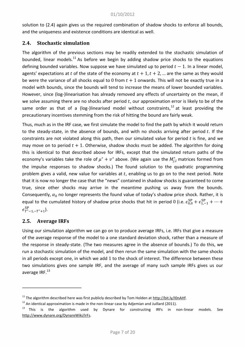
The fall in domestic demand induces output in both countries to fall. This leads to falling inflation in both countries and hence the central banks decrease the interest rates to boost demand. However, in the presence of the ZLB, the central banks are unable to decrease the interest rate strongly enough to generate a negative real interest rate, and consequently the recession is even more severe. This is further amplified by even larger downturns of both inflation rates. Since the foreign nominal interest rate hits the ZLB, a strong foreign recession is generated, despite the model’s  otherwise feeble transmission mechanism. Producing Figure 1 took roughly a half second on a standard desktop PC, illustrating just how low is the computation cost of imposing the ZLB.

In Figure 2 we go on to simulate this model (with the standard deviation of both shocks set equal to 0.2), for 220 quarters, dropping the first 100, a process that took less than two seconds. The shaded areas of the figure show periods when both bounds are hit simultaneously, illustrating that recessions become substantially more severe in these situations.

Figure 2: Simulations from the two-country model of Clarida et al. (2002).

(Dashed line imposes the ZLB, solid line does not.)21

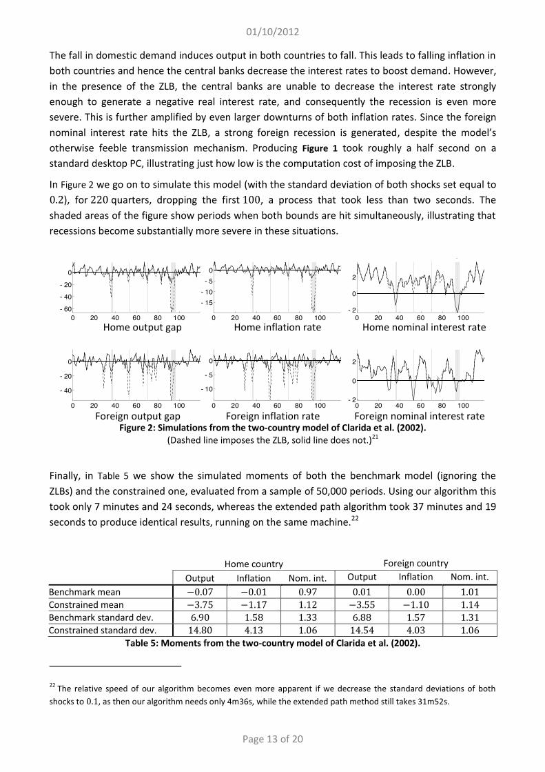
Finally, in Table 5 we show the simulated moments of both the benchmark model (ignoring the ZLBs) and the constrained one, evaluated from a sample of 50,000 periods. Using our algorithm this took only 7 minutes and 24 seconds, whereas the extended path algorithm took 37 minutes and 19 seconds to produce identical results, running on the same machine.22

Home country Foreign country Output Inflation Nom. int. Output Inflation Nom. int.

Benchmark mean −0.07 −0.01 0.97 0.01 0.00 1.01 Constrained mean −3.75 −1.17 1.12 −3.55 −1.10 1.14 Benchmark standard dev. 6.90 1.58 1.33 6.88 1.57 1.31 Constrained standard dev. 14.80 4.13 1.06 14.54 4.03 1.06

Table 5: Moments from the two-country model of Clarida et al. (2002).

22 The relative speed of our algorithm becomes even more apparent if we decrease the standard deviations of both shocks to 0.1, as then our algorithm needs only 4m36s, while the extended path method still takes 31m52s.

0 5 10

- 60

- 40

- 20

0

0 5 10

- 20

- 15

- 10

- 5

0

0 5 10

- 0.5

0

0.5

0 5 10- 50

- 40

- 30

- 20

- 10

0

0 5 10

- 12

- 10

- 8

- 6

- 4

- 2

0

0 5 10

0.7

0.8

0.9

1

0 20 40 60 80 100- 60

- 40

- 20

0

0 20 40 60 80 100

- 15- 10

- 50

0 20 40 60 80 100- 2

0

2

0 20 40 60 80 100

- 40

- 20

0

0 20 40 60 80 100

- 10

- 5

0

0 20 40 60 80 100- 2

0

2

0 5 10

- 60

- 40

- 20

0

0 5 10

- 20

- 15

- 10

- 5

0

0 5 10

- 0.5

0

0.5

0 5 10- 50

- 40

- 30

- 20

- 10

0

0 5 10

- 12

- 10

- 8

- 6

- 4

- 2

0

0 5 10

0.7

0.8

0.9

1

0 20 40 60 80 100- 60

- 40

- 20

0

0 20 40 60 80 100

- 15- 10

- 50

0 20 40 60 80 100- 2

0

2

0 20 40 60 80 100

- 40

- 20

0

0 20 40 60 80 100

- 10

- 5

0

0 20 40 60 80 100- 2

0

2

Foreign output gap Foreign inflation rate Foreign nominal interest rate

Home output gap Home inflation rate Home nominal interest rate

01/10/2012

Page 14 of 20

Table 5 makes clear the magnitude of the increase in the volatility of both output gaps and inflation when we impose the ZLB on interest rates, as well as the large recessionary impact.23 We stress again that we do not claim these values to be realistic. Rather, we presented the previous graphs and Table 5 to make clear the importance of the ZLB, and underline the tiny cost of imposing it using the method proposed in this paper.

Having shown the workings of the algorithm in a very stylized example, we now turn to a more realistic application, using the seminal Smets and Wouters (2003) model of the Euro Area.

4.2. The ZLB in the Smets and Wouters (2003) model

Modern macroeconomic models are getting progressively larger, so it is important that our algorithm can handle big models, of which the Smets and Wouters (2003) model is the canonical example. It also enables us to get a more realistic impression of the importance of the ZLB for the analysis of DSGE models.

We briefly recap the features of the model, but refer the reader to the paper for further details. It features sticky prices and wages, capital adjustment costs, variable capital utilisation and habit formation in consumption. The stochastic side of the model consists of ten exogenous shocks: six persistent shocks (technology, investment, preferences, labor supply, government spending and an inflation objective shock), all modelled as standard AR(1) -processes, and four short-run i.i.d. shocks (wage mark-ups, price mark-ups, Tobin's Q, and a monetary policy shock).

Since the original paper uses detrended data for estimation, the inflation target is set to zero. As this implies a very low steady state interest rate, we would find ourselves at the ZLB implausibly often. Hence, we add a positive annual inflation target of 1.8% to the Taylor rule, implying a quarterly steady state interest rate of 1.451%. Since the official target of the ECB is below, but near 2%, we believe this to be an adequate  representation  of  Europe’s monetary policy. All other model parameters are calibrated according to the reported posterior mode in Smets and Wouters (2003).24

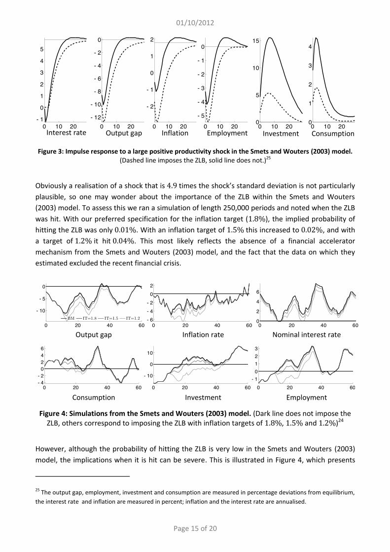
Smets and Wouters (2003) find that preference and productivity shocks are the chief drivers of fluctuations in nominal interest rates. It makes sense then to look at productivity shocks to illustrate how things change when the ZLB is imposed. In Figure 3, we plot the IRF to a large positive productivity shock (4.9 times   the   shock’s   estimated   standard   deviation).   Since   natural   output  increases faster than actual output, this produces a large negative output gap, and the ZLB is hit. Hitting the ZLB dampens the response of investment, and so rather than output returning to trend within four years (as it would in the absence of the ZLB), instead it takes around eight years for the output gap to close.

23 Obviously, the assumption of completely symmetric countries implies that the moments of domestic and foreign variables should converge to equal values as we increase the number of periods. 24 The model code is taken from the extensive model database described in Cwik et al. (2012).

01/10/2012

Page 15 of 20

Figure 3: Impulse response to a large positive productivity shock in the Smets and Wouters (2003) model.

(Dashed line imposes the ZLB, solid line does not.)25

Obviously a realisation of a shock that is 4.9 times  the  shock’s  standard  deviation  is  not  particularly  plausible, so one may wonder about the importance of the ZLB within the Smets and Wouters (2003) model. To assess this we ran a simulation of length 250,000 periods and noted when the ZLB was hit. With our preferred specification for the inflation target (1.8%), the implied probability of hitting the ZLB was only 0.01%. With an inflation target of 1.5% this increased to 0.02%, and with a target of 1.2% it hit 0.04%. This most likely reflects the absence of a financial accelerator mechanism from the Smets and Wouters (2003) model, and the fact that the data on which they estimated excluded the recent financial crisis.

Figure 4: Simulations from the Smets and Wouters (2003) model. (Dark line does not impose the

ZLB, others correspond to imposing the ZLB with inflation targets of 1.8%, 1.5% and 1.2%)24

However, although the probability of hitting the ZLB is very low in the Smets and Wouters (2003) model, the implications when it is hit can be severe. This is illustrated in Figure 4, which presents

25 The output gap, employment, investment and consumption are measured in percentage deviations from equilibrium, the interest rate and inflation are measured in percent; inflation and the interest rate are annualised.

0 10 20- 1

0

1

2

3

4

5

0 10 20- 12

- 10

- 8

- 6

- 4

- 2

0

0 10 20

- 2

- 1

0

1

2

0 10 20

- 5

- 4

- 3

- 2

- 1

0

0 10 200

5

10

15

0 10 200

1

2

3

4

0 20 40 60

- 10

- 5

0

0 20 40 60- 6- 4- 2

02

0 20 40 600

2

4

6

0 20 40 60- 4- 2

0246

0 20 40 60

- 10

0

10

0 20 40 60- 1

0123

0 20 40 60

- 10

- 5

0

0 20 40 60- 6- 4- 2

02

0 20 40 600

2

4

6

0 20 40 60- 4- 2

0246

0 20 40 60

- 10

0

10

0 20 40 60- 1

0123

Interest rate Output gap Inflation Employment Investment Consumption

Output gap Inflation rate Nominal interest rate

Consumption Investment Employment

01/10/2012

Page 16 of 20

simulated paths for a period of 15 years during which the ZLB was hit. This figure also illustrates the increasing effect of the ZLB as the inflation target is decreased.

The solid black line represents the benchmark scenario, ignoring the bound; the grey lines represent scenarios with a ZLB for different inflation targets (the lighter the line, the lower the inflation target). For a 1.8% percent inflation target, the ZLB is hit in the 13th quarter, and holds for

only two periods. In this case, the simulated path is nearly identical to the benchmark one ignoring the ZLB. However, the lower the inflation target, the more severe is the fall in prices and aggregate activity. For an inflation target of 1.2%, the ZLB binds for one year. During this period, monetary

policy is unable to prevent a drop in investment, resulting in investment staying below equilibrium for eleven and a half years. Moreover, employment stays below its long-term steady state for about

nine years. The conclusion of this exercise is that with a high enough inflation target, hitting the ZLB is incredibly unlikely, and so the expected welfare loss from the bound is minimal. However, once the bound is hit, the impact can be very strong and highly persistent, as we are presently seeing in

reality.

Finally, the Smets and Wouters (2003) model gives us another opportunity to present our algorithm’s   speed   advantage.   With   the   first   two   inflation   targets,   our   algorithm   only   took   10  minutes and 33 seconds, for 250,000 periods, rising to 22 minutes and 17 seconds with an inflation target of 1.2%. By contrast, the extended path algorithm of Adjemian and Juillard (2011) took 3

hours and 45 minutes just to simulate 50000 periods, after which it crashed. Clearly, only our algorithm is viable on models of the scale of Smets and Wouters (2003).

5. Conclusion This paper provides a fast, simple and intuitive method for the simulations of DSGE models with inequality  constraints,  based  on  the  introduction  of  “shadow  price  shocks”  which  hit  the  bounded  variables whenever the constraints are violated. We showed that at second order, the algorithm is

more accurate than all methods except fully global ones, and we showed that the second order algorithm also leads in terms of speed, at least when compared to other algorithms of similar

accuracy. At first order we illustrated that the speed was even greater, enabling it to be reliably used on the largest models around today.

We believe our algorithm will prove useful to a very wide variety of models including bounded

variables, and we hope to investigate its application to the estimation of such models in future work.

01/10/2012

Page 17 of 20

6. References Adjemian, Stéphane, Houtan Bastani, Michel Juillard, Ferhat Mihoubi, George Perendia, Marco

Ratto, and Sébastien Villemot. 2011. Dynare: Reference Manual, Version 4. Dynare Working Papers. CEPREMAP, April. http://ideas.repec.org/p/cpm/dynare/001.html.

Adjemian, Stéphane, and Michel Juillard. 2011. Accuracy of the Extended Path Simulation Method in

a New Keynesian Model with a Zero Lower Bound on the Nominal Interest Rate. Mimeo. Braun, R. Anton, and Lena Mareen Körber. 2011. New Keynesian Dynamics in a Low Interest Rate

Environment. Journal of Economic Dynamics and Control 35, no. 1: 2213–2227. Braun, R. Anton, Lena Mareen Körber, and Yuichiro Waki. 2012. Some unpleasant properties of log-

linearized solutions when the nominal rate is zero. Working Paper. Federal Reserve Bank of Atlanta. http://ideas.repec.org/p/fip/fedawp/2012-05.html.

Chen, Qianying, Michael Funke, and Michael Paetz. 2012. Market and Non-Market Monetary Policy

Tools in a Calibrated DSGE Model for Mainland China. BOFIT Discussion Papers. Bank of Finland, Institute for Economies in Transition, July. http://ideas.repec.org/p/hhs/bofitp/2009_014.html.

Christiano, L. J., M. Eichenbaum, and S. Rebelo. 2011. When is the Government Multiplier Large. Journal of Political Economy 119: 78–121.

Clarida, R., J. Galí, and M. Gertler. 1999. The Science of Monetary Policy: A New Keynesian Perspective. Journal of Economic Literature 37: 1661–1701.

———. 2002. A Simple Framework for International Monetary Policy Analysis. Journal of Monetary

Economics 49, no. 5: 879–904. Coenen, G., A. Orphanides, and V. Wieland. 2004. Price Stability and Monetary Policy Effectiveness

when Nominal Interest Rates are Bounded at Zero. The B.E. Journal of Macroeconomics 4, no. 1: -.

Cwik, Tobias, Gernot Mueller, Sebastian Schmidt, Volker Wieland, and Maik H. Wolters. 2012. A New Comparative Approach to Macroeconomic Modeling and Policy Analysis. forthcoming

in Journal of Economic Behavior and Organization. Eggertsson, Gauti B., and Michael Woodford. 2003. The Zero Bound on Interest Rates and Optimal

Monetary Policy. Brookings Papers on Economic Activity 34, no. 1: 139–235. Erceg, Christopher J., and Jesper Lindé. 2010. Is there a fiscal free lunch in a liquidity trap?

International Finance Discussion Papers. Board of Governors of the Federal Reserve System (U.S.). http://ideas.repec.org/p/fip/fedgif/1003.html.

Fernández-Villaverde, Jesús, Grey Gordon, Pablo A. Guerrón-Quintana, and Juan Rubio-Ramírez. 2012. Nonlinear Adventures at the Zero Lower Bound. NBER Working Papers. National Bureau of Economic Research, Inc, May. http://ideas.repec.org/p/nbr/nberwo/18058.html.

Fernández-Villaverde, Jesús, and Juan Rubio-Ramírez. 2010. Macroeconomics and Volatility: Data,

Models, and Estimation. NBER Working Papers. National Bureau of Economic Research, Inc, December. http://ideas.repec.org/p/nbr/nberwo/16618.html.

Fuhrer, Jeffrey C., and Brian F. Madigan. 1997. Monetary Policy When Interest Rates Are Bounded At Zero. The Review of Economics and Statistics 79, no. 4 (November): 573–585.

Funke, Michael, and Michael Paetz. 2012. A DSGE-Based Assessment of Nonlinear Loan-to-Value

Policies: Evidence from Hong Kong. BOFIT Discussion Papers. Bank of Finland, Institute for Economies in Transition, May. http://ideas.repec.org/p/hhs/bofitp/2012_011.html.

Galí, J., and M. Gertler. 1999. Inflation Dynamics: A Structural Econometric Analysis. Journal of

Monetary Economics 44: 195–222. Guerrieri, Luca, and Matteo Iacoviello. 2012. A Toolkit to Solve Models with Occasionally Binding

Constraints Easily. September 21.

01/10/2012

Page 18 of 20

Holden, Tom. 2010. Products, patents and productivity persistence: A DSGE model of endogenous growth. Economics Series Working Paper. University of Oxford, Department of Economics. http://ideas.repec.org/p/oxf/wpaper/512.html.

Juillard, Michel. 2011. Local approximation of DSGE models around the risky steady state. Wp.comunite. Department of Communication, University of Teramo. http://ideas.repec.org/p/ter/wpaper/0087.html.

Jung, Taehun, Yuki Teranishi, and Tsutomu Watanabe. 2005. Optimal Monetary Policy at the Zero-Interest-Rate Bound. Journal of Money, Credit and Banking 37, no. 5 (October 1): 813–835.

Kim, Sunghyun Henry, Jinill Kim, Ernst Schaumburg, and Christopher A. Sims. 2008. Calculating and Using Second Order Accurate Solutions of Discrete Time Dynamic Equilibrium Models. Journal of Economic Dynamics and Control 32, no. 11: 3397–3414.

Krueger, Dirk, Felix Kubler, and Benjamin A. Malin. 2011. Solving the multi-country real business cycle model using a Smolyak-collocation method. Journal of Economic Dynamics and Control 35, no. 2 (February): 229–239.

Maliar, Serguei, Lilia Maliar, and Kenneth Judd. 2011. Solving the multi-country real business cycle model using ergodic set methods. Journal of Economic Dynamics and Control 35, no. 2 (February): 207–228.

Rotemberg, Julio J. 1996. Prices, output, and hours: An empirical analysis based on a sticky price model. Journal of Monetary Economics 37, no. 3 (June): 505–533.

Smets, F., and R. Wouters. 2003. An Estimated Dynamic Stochastic General Equilibrium Model for the Euro Area. Journal of the European Economic Association 1, no. 5.

01/10/2012

Page 19 of 20

7. Online appendices

7.1. The NK model of Fernández-Villaverde et al. (2012)

Households choose consumption 𝐶 and labour supply 𝐿 to maximise their utility, given the wage 𝑊 , the rate of inflation Π and the nominal interest rate 𝑅 . This leads to the FOCs:

1𝐶

= 𝔼𝛽 𝑅𝐶 Π

, 𝜓𝐿 𝐶 = 𝑊 .

Firms choose prices to maximise profits. This leads them to set a relative price Π∗ satisfying:

MC =𝑊𝐴

, 𝜀𝑥 , = (𝜀 − 1)𝑥 , ,

𝑥 , =MC 𝑌𝐶

+ 𝜃𝔼 𝛽 Π 𝑥 , , 𝑥 , = Π∗ 𝑌𝐶

+ 𝜃𝔼 𝛽ΠΠ∗ 𝑥 , ,

where 𝐴 is productivity, MC is marginal costs and 𝑌 is output.

The central bank follows a standard Taylor rule, with monetary policy shock 𝑀 , and government spending is a stochastic fraction 𝑆 , of total output:

𝑅 = max 1, 𝑅 𝑅ΠΠ

𝑌𝑌

𝑀 , 𝐺 = 𝑆 , 𝑌 .

Inflation and price dispersion evolve according to:

1 = 𝜃Π + (1 − 𝜃)(Π∗) , 𝜐 = 𝜃Π + (1 − 𝜃)(Π∗) .

Finally, market clearing in goods and labour markets imply:

𝑌 = 𝐶 + 𝐺 , 𝑌 =𝐴 𝐿𝜐

.

The stochastic processes 𝛽 , 𝐴 , 𝑀 and 𝑆 , are all log AR(1).

7.2. Our modified version of the two-country model of Clarida et al. (2002)

Let 𝑦 , 𝜋 and 𝑖 represent the domestic output gap, inflation rate and interest rate respectively, and let 𝑦∗, 𝜋∗ and 𝑖∗ denote their foreign equivalents. Let 𝜈 and 𝜈∗ be home and foreign demand shocks. When both countries are symmetric, the linearised model is described by the following four equations, and another four in which the roles of home and foreign country are swapped:

𝑦 = 𝔼 𝑦 − 𝜎 (𝑖 − 𝔼 𝜋 − 𝜅 𝔼 Δ𝑦∗ + 𝜅 (1 − 𝜌 )𝜈 − 𝚤)̅,

𝜋 = Φ(𝜃𝛽𝔼 𝜋 + 𝜏𝜋 ) + 𝜆𝑦 ,

𝑖 = max 0, 𝚤̅ + (1 − 𝜙 ) 𝜙 𝜋 + 𝜙 𝑦 + 𝜙 (𝑖 − 𝚤)̅ ,

𝜈 = 𝜌 𝜈 + 𝜀 .

These represent the Euler equation, the NK Phillips curve, the Taylor rule and the evolution of the exogenous shock, respectively.

01/10/2012

Page 20 of 20

The parameters used in the equations above are the following functions of the structural parameters:

𝜅 =𝜎 − 12

, 𝜎 = 𝜎 − 𝜅 , 𝜅 = 𝜎 − 𝜅 + 𝜑, 𝜆 =(1 − 𝜃)(1 − 𝛽𝜃)

𝜃𝜅, 𝚤̅ =

1𝛽

Φ =1

𝜃 + 𝜏 1 − 𝜃(1 − 𝛽),

where 𝜎 ≔ 13 is the inverse elasticity of intertemporal substitution in consumption,26 𝜑 ≔ 1 is

the inverse Frisch elasticity of labour supply, 𝛽 ≔ 0.99 is the discount factor, 𝜃 ≔ 34 is the

probability  a  firm’s  price  must  remain  fixed and 𝜏 ≔ 110 is the fraction of backwards looking price

setters. We also set 𝜙 ≔ 1.5, 𝜙 ≔ 0.125 and 𝜙 ≔ 0.8 in the   central   bank’s   reaction   function  and  the  shocks’  persistence  as  𝜌 ≔ 0.7.

26 The model implicitly assumes a unitary substitution elasticity between domestic and foreign goods. Hence, for values of 𝜎 smaller than one, any increase in foreign production is accompanied by an increase in domestic production, since the negative effect due to the implied real appreciation is dominated by the fall in the real interest rate stemming from an increase in domestic consumer price inflation. With 𝜎 = 1 (i.e. log utility) both effects balance each other out, since in that case 𝜅 = 0, meaning there is no transmission at all. We could derive similar results for lower substitution elasticities and higher values of 𝜎, but we maintain this parameterisation to keep the model close to that of Clarida et al. (2002).