disinfection profiling and benchmarking
TRANSCRIPT

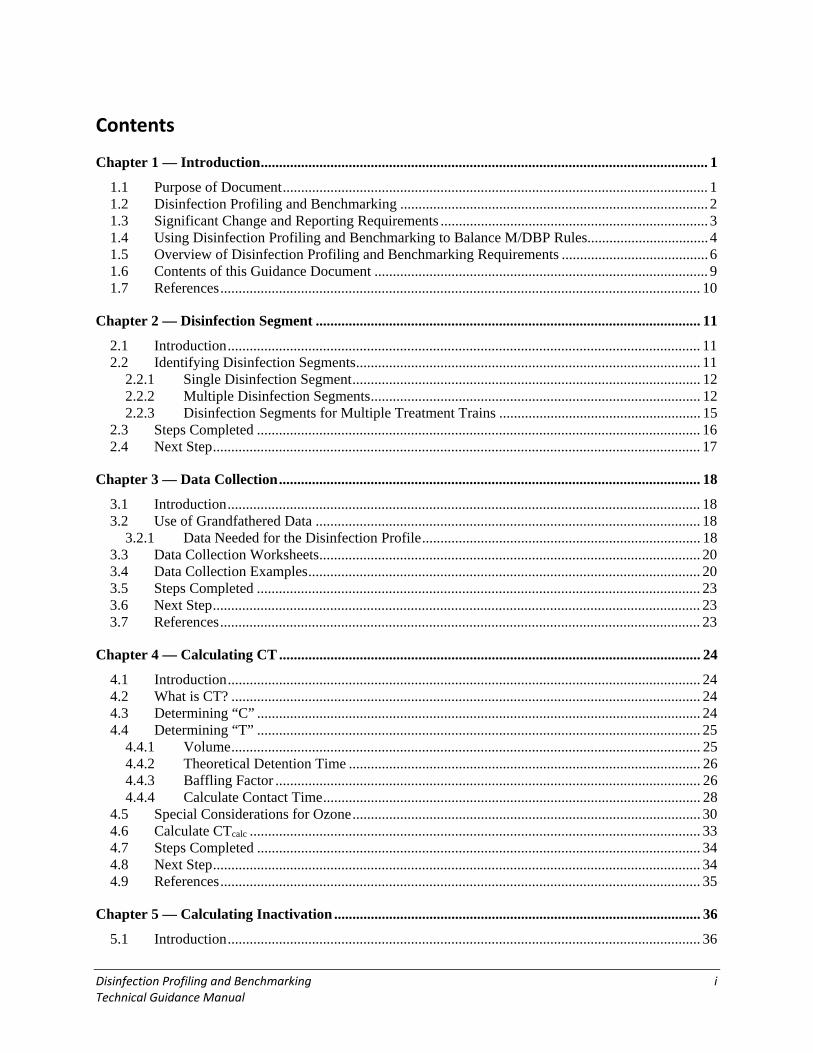
Disinfection Profiling and Benchmarking
Technical Guidance Manual
0.000
0.200
0.400
0.600
0.800
1.000
1.200
1.400
0 4 8 12 16 20 24 28 32 36 40 44 48 52
Log
Inac
tivat
ion Log Inactivation
Benchmark
Week Tested

Office of Water (4606M) EPA 815-R-20-003 June 2020

Disclaimer
This document provides guidance to states, tribes and the U.S. Environmental Protection Agency (EPA) exercising primary enforcement responsibility under the Safe Drinking Water Act (SDWA) and contains the EPA’s current policy recommendations for complying with the disinfection profiling and benchmarking requirements of the suite of Surface Water Treatment Rules (SWTRs). Throughout this document, the terms “state” and “states” are used to refer to all types of primacy agencies including states, U.S. territories, American Indian tribes and the EPA. The statutory provisions and the EPA regulations described in this document are legally binding requirements. This document, however, is not a regulation itself, nor does it change or substitute for those provisions and regulations. Thus, it does not impose legally binding requirements on the EPA, states, or the regulated community. This guidance does not confer legal rights or impose legal obligations upon any member of the public. While the EPA has made every effort to ensure the accuracy of the discussion in this guidance, the obligations of the regulated community are determined by statutes, regulations, or other legally binding requirements. In the event of a conflict between the discussion in this document and any statute or regulation, this document would not be controlling. The general description provided here may not apply to a particular situation based upon the circumstances. Interested parties are free to raise questions and objections about the substance of this guidance and the appropriateness of the application of this guidance to a particular situation. The EPA and other decision makers retain the discretion to adopt approaches on a case-by-case basis that differ from those described in this guidance, where appropriate. Mention of trade names or commercial products does not constitute endorsement or recommendation for their use. This is a living document and may be revised periodically without public notice. The EPA welcomes public input on this document at any time.

This Page Intentionally Left Blank
Disinfection Profiling and Benchmarking i Technical Guidance Manual
Contents
Chapter 1 — Introduction .......................................................................................................................... 1
1.1 Purpose of Document .................................................................................................................... 1 1.2 Disinfection Profiling and Benchmarking .................................................................................... 2 1.3 Significant Change and Reporting Requirements ......................................................................... 3 1.4 Using Disinfection Profiling and Benchmarking to Balance M/DBP Rules................................. 4 1.5 Overview of Disinfection Profiling and Benchmarking Requirements ........................................ 6 1.6 Contents of this Guidance Document ........................................................................................... 9 1.7 References ................................................................................................................................... 10
Chapter 2 — Disinfection Segment ......................................................................................................... 11
2.1 Introduction ................................................................................................................................. 11 2.2 Identifying Disinfection Segments .............................................................................................. 11
2.2.1 Single Disinfection Segment ............................................................................................... 12 2.2.2 Multiple Disinfection Segments .......................................................................................... 12 2.2.3 Disinfection Segments for Multiple Treatment Trains ....................................................... 15
2.3 Steps Completed ......................................................................................................................... 16 2.4 Next Step ..................................................................................................................................... 17
Chapter 3 — Data Collection ................................................................................................................... 18
3.1 Introduction ................................................................................................................................. 18 3.2 Use of Grandfathered Data ......................................................................................................... 18
3.2.1 Data Needed for the Disinfection Profile ............................................................................ 18 3.3 Data Collection Worksheets ........................................................................................................ 20 3.4 Data Collection Examples ........................................................................................................... 20 3.5 Steps Completed ......................................................................................................................... 23 3.6 Next Step ..................................................................................................................................... 23 3.7 References ................................................................................................................................... 23
Chapter 4 — Calculating CT ................................................................................................................... 24
4.1 Introduction ................................................................................................................................. 24 4.2 What is CT? ................................................................................................................................ 24 4.3 Determining “C” ......................................................................................................................... 24 4.4 Determining “T” ......................................................................................................................... 25
4.4.1 Volume ................................................................................................................................ 25 4.4.2 Theoretical Detention Time ................................................................................................ 26 4.4.3 Baffling Factor .................................................................................................................... 26 4.4.4 Calculate Contact Time ....................................................................................................... 28
4.5 Special Considerations for Ozone ............................................................................................... 30 4.6 Calculate CTcalc ........................................................................................................................... 33 4.7 Steps Completed ......................................................................................................................... 34 4.8 Next Step ..................................................................................................................................... 34 4.9 References ................................................................................................................................... 35
Chapter 5 — Calculating Inactivation .................................................................................................... 36
5.1 Introduction ................................................................................................................................. 36

Disinfection Profiling and Benchmarking ii Technical Guidance Manual
5.2 CT Tables .................................................................................................................................... 36 5.3 Determining CT Required ........................................................................................................... 36
5.3.1 CT99.9 for Giardia ................................................................................................................ 37 5.3.2 CT99.99 for Viruses ............................................................................................................... 40
5.4 Calculating Log Inactivation for One Disinfection Segment ...................................................... 40 5.5 Calculating Log Inactivation for Multiple Disinfection Segments ............................................. 42 5.6 Available Spreadsheets ............................................................................................................... 46 5.7 Steps Completed ......................................................................................................................... 46 5.8 Next Step ..................................................................................................................................... 46
Chapter 6 — Developing the Disinfection Profile and Benchmark ...................................................... 47
6.1 Introduction ................................................................................................................................. 47 6.2 Constructing a Disinfection Profile ............................................................................................. 47 6.3 Calculating the Disinfection Benchmark .................................................................................... 50 6.4 Seasonal Variations ..................................................................................................................... 52 6.5 The Complete Profile and Benchmark ........................................................................................ 54 6.6 Steps Completed ......................................................................................................................... 54 6.7 Next Step ..................................................................................................................................... 54
Chapter 7 — Evaluating Disinfection Practice Modifications .............................................................. 55
7.1 Introduction ................................................................................................................................. 55 7.2 Significant Changes to Disinfection Practices ............................................................................ 55
7.2.1 Changes to the Point of Disinfection .................................................................................. 55 7.2.2 Changes to Disinfectant Type ............................................................................................. 56 7.2.3 Changes to the Disinfection Process ................................................................................... 58 7.2.4 Other Modifications ............................................................................................................ 58
7.3 How the State Will Use the Benchmark ..................................................................................... 59 7.4 Steps Completed ......................................................................................................................... 60 7.5 References ................................................................................................................................... 60
Chapter 8 — Treatment Considerations ................................................................................................ 61
8.1 Introduction ................................................................................................................................. 61 8.2 Alternative Disinfectants and Oxidants ...................................................................................... 61
8.2.1 Chloramines (NH2Cl) .......................................................................................................... 61 8.2.2 Ozone (O3) .......................................................................................................................... 62 8.2.3 Chlorine Dioxide (ClO2) ..................................................................................................... 62 8.2.4 Potassium Permanganate (KMnO4) .................................................................................... 63 8.2.5 Ultraviolet Radiation (UV) ................................................................................................. 64 8.2.6 Comparison of Disinfectants ............................................................................................... 65
8.3 Changes in Enhanced Coagulation and Softening ...................................................................... 66 8.4 Increasing Contact Time ............................................................................................................. 67 8.5 Membranes .................................................................................................................................. 68 8.6 References ................................................................................................................................... 69

Disinfection Profiling and Benchmarking iii Technical Guidance Manual
Appendices
Appendix A — Glossary ........................................................................................................................... A-1
Appendix B — CT Tables ........................................................................................................................ B-1
Appendix C — Blank Worksheets ............................................................................................................ C-1
Appendix D — Examples ......................................................................................................................... D-1
Appendix E — Tracer Studies .................................................................................................................. E-1
Appendix F — Calculating the Volume of Each Sub-Unit ....................................................................... F-1
Appendix G — Baffling Factors ............................................................................................................... G-1
Appendix H — Conservative Estimate, Interpolation and Regression Method Examples ....................... H-1
Figures
Figure 1-1. Sample Disinfection Profile ....................................................................................................... 2
Figure 1-2. Steps in Developing a Disinfection Profile and Benchmark ...................................................... 3
Figure 1-3. LT2ESWTR Disinfection Profile and Benchmark Decision Tree ............................................. 8
Figure 2-1. Plant Schematic Showing a Conventional Filtration Plant with One Disinfection Segment ... 12
Figure 2-2. Plant Schematic Showing a Conventional Filtration Plant with Two Disinfection Segments ..................................................................................................................................................... 13
Figure 2-3. Plant Schematic Showing One Injection Point with Multiple Disinfection Segments ............. 14
Figure 2-4. Plant Schematic Showing Two Injection Points with Multiple Disinfection Segments .......... 14
Figure 2-5. Plant Schematic Showing Two Identical Treatment Trains and Each with Multiple Disinfection Segments ................................................................................................................................ 15
Figure 2-6. Plant Schematic Showing Two Treatment Trains with Different Flows and Each with Multiple Disinfection Segments.................................................................................................................. 16
Figure 4-1. Baffling Characteristics of a Pipe and Clearwell ..................................................................... 27
Figure 6-1. Example of a Completed Disinfection Profile ......................................................................... 47
Figure 6-2. 2014 Data ................................................................................................................................. 53
Figure 6-3. 2015 Data ................................................................................................................................. 53
Figure 6-4. 2016 Data ................................................................................................................................. 53

Disinfection Profiling and Benchmarking iv Technical Guidance Manual
Figure 7-1. Example of Moving the Point of Pre-disinfectant Application ................................................ 56
Figure 7-2. Example of Changing Disinfectant Type ................................................................................. 57
Figure 7-3. Changing Pre-disinfection Location and Type of Disinfectant ................................................ 57
Figure 8-1. Particles Removed Through Membrane Technologies ............................................................ 69
Tables
Table 1-1. Minimum Removal and Inactivation Requirements for All Surface Water and GWUDI Filtered Systems ............................................................................................................................................ 4
Table 1-2. Typical Removal Credits and Inactivation Requirements for Various Treatment Technologies ................................................................................................................................................. 5
Table 4-1. Volume Equations for Shapes ................................................................................................... 26
Table 4-2. Baffling Factors ......................................................................................................................... 27
Table 4-3. Correlations to Predict C* Based on Ozone Residual Concentrations in the Outlet of a Chamber ...................................................................................................................................................... 31
Table 5-1. Excerpt from Table B-1 ............................................................................................................. 39
Table 8-1. Study Results on Changing Primary and Secondary Disinfectants ........................................... 65
Examples
Example 3-1. Collecting Data for a Single Segment .................................................................................. 21
Example 3-2. Collecting Data for Multiple Disinfection Segments ........................................................... 22
Example 4-1. Determining “T” for a clearwell with no baffling ................................................................ 28
Example 4-2. Calculate CTcalc ..................................................................................................................... 33
Example 5-1. Determining CT99.9 Disinfection with Chlorine .................................................................... 38
Example 5-2. Determining Log Inactivation for Giardia for a PWS with One Disinfection Segment ...... 41
Example 5-3. Determining Total Log Giardia Inactivation for PWS with Multiple Disinfection Segments ..................................................................................................................................................... 43
Example 6-1. Disinfection Profile for Giardia ........................................................................................... 48
Example 6-2. Calculating a Disinfection Benchmark ................................................................................. 50
Disinfection Profiling and Benchmarking v Technical Guidance Manual
Acronyms
List of common abbreviations and acronyms used in this document:
AMWA Association of Metropolitan Water Agencies
AWWA American Water Works Association
APHA American Public Health Association
BF Baffling Factor
C Concentration
CFR Code of Federal Regulations
CSTR Continuous Stirred Reactor Method
CT Concentration x Time
CWS Community Water System
DBP Disinfection Byproduct
DBPRs Disinfectants and Disinfection Byproducts Rules
DOM Dissolved Organic Matter
DPD N, N-diethyl-p-phenylenediamine
EPA Environmental Protection Agency
ft Feet
gal Gallons
gpm Gallons per Minute
GWUDI Ground Water Under the Direct Influence of Surface Water
HAA5 Haloacetic Acids (Five Regulated)
HDT Hydraulic detention time
IESWTR Interim Enhanced Surface Water Treatment Rule
LRAA Locational running annual average
LT1ESWTR Long Term 1 Enhanced Surface Water Treatment Rule
LT2ESWTR Long Term 2 Enhanced Surface Water Treatment Rule
MCL Maximum Contaminant Level
mg/L Milligrams per Liter
MRDL Maximum Residual Disinfectant Level
NTNCWS Non-transient Non-community Water System
PWS Public Water System
Q Peak Hourly Flow Rate
RED Reduction equivalent dose
SCADA Supervisory Control and Data Acquisition
Disinfection Profiling and Benchmarking vi Technical Guidance Manual
SDWA Safe Drinking Water Act
Stage 1 DBPR Stage 1 Disinfectants and Disinfection Byproducts Rule
Stage 2 DBPR Stage 2 Disinfectants and Disinfection Byproducts Rule
SWTR Surface Water Treatment Rule
T Contact Time
TDT Theoretical Detention Time
TNCWS Transient Non-community Water System
TOC Total Organic Carbon
TTHM Total Trihalomethanes
UV Ultraviolet
UVT UV transmittance
USEPA United States Environmental Protection Agency
V Volume
X log inactivation Reduction to 1/10x of original concentration by disinfection
X log removal Reduction to 1/10x of original concentration by physical removal
μm Micron (10-6 meter)
UVDGM Ultraviolet Disinfection Guidance Manual

Disinfection Profiling and Benchmarking 1 Technical Guidance Manual
Chapter 1 — Introduction Under the Safe Drinking Water Act (SDWA), the Environmental Protection Agency (EPA) has developed interrelated regulations to control microbial pathogens, disinfectants, and disinfection byproducts (DBPs) in drinking water. These rules, collectively known as the microbial/disinfection byproducts (M/DBP) rules, primarily address two key public health concerns: acute threats from microbial contamination and chronic threats from disinfectant residuals and byproducts of disinfection. The EPA recognizes that a public water system (PWS) may encounter compliance issues when trying to simultaneously meet the goals of the following M/DBP rules:
• Surface Water Treatment Rule (SWTR); • Interim Enhanced Surface Water Treatment Rule (IESWTR); • Long Term 1 Enhanced Surface Water Treatment Rule (LT1ESWTR); • Long Term 2 Enhanced Surface Water Treatment Rule (LT2ESWTR); and • Stage 1 and Stage 2 Disinfectants and Disinfection Byproducts Rules (DBPRs).
Modifications to improve microbial treatment to comply with the SWTR, IESWTR, LT1ESWTR, and LT2ESWTR may adversely affect compliance with the Stage 1 DBPR and Stage 2 DBPR and vice versa. In addition to the challenges of simultaneously complying with this suite of M/DBP rules, a PWS must ensure that changes in treatment do not adversely affect compliance with other drinking water regulations and environmental regulations.
Simultaneous compliance with the M/DBP rules may present a significant challenge to PWSs and require them to reconsider their disinfection practices. But prior to making any significant modifications to their existing disinfection practices, PWSs should clearly understand the impact those changes could have on microbial protection. Disinfection profiling and benchmarking are procedures by which PWSs and state drinking water programs (referred to as “states” in this document), working together, can ensure that there will be no significant reduction in microbial protection as a result of modifying disinfection practices to maintain compliance with other regulations.
1.1 Purpose of Document
This guidance manual has been updated from the original technical guidance for disinfection profiling and benchmarking requirements pertaining to the IESWTR and LT1ESWTR, which apply to PWSs supplied by a surface water source or ground water source that is under the direct influence of surface water. It has been updated to help PWSs comply with the disinfection profiling and benchmarking requirements of the LT2ESWTR. This manual explains disinfection profiling and benchmarking, discusses when and why they are necessary, and provides guidance on how to collect data to calculate them. This manual also discusses how PWSs and states may use these data to make decisions about disinfection practices and provides an overview of different treatment practices that PWSs may consider adopting.
Additional copies of this document may be obtained by:
• Contacting the appropriate state office. • Downloading from the EPA’s website at https://www.epa.gov/dwreginfo/guidance-manuals-
surface-water-treatment-rules. • Contacting the EPA by filling out an online form on the EPA Safe Drinking Water Information
website at https://www.epa.gov/ground-water-and-drinking-water/safe-drinking-water-information.

Disinfection Profiling and Benchmarking 2 Technical Guidance Manual
1.2 Disinfection Profiling and Benchmarking
Disinfection is a critical element in controlling the transmission of disease from drinking water by inactivating disease-causing pathogens, such as bacteria, protozoa, and viruses that can affect human health.
The strength of a chemical disinfectant (e.g., chlorine, chlorine dioxide, ozone) for inactivating pathogens when in contact with water can be measured by its CT value. 1
1 CT is defined as disinfectant residual concentration (C) multiplied by contact time (T). A CT value is a measure of disinfection effectiveness for the time that microorganisms in the water are in contact with a disinfectant. See Chapter 4 for a discussion on CT values and how they are calculated.
Methods for determining CT based onoperational data are described in Chapters 3 and 4. The CT values are used to evaluate the inactivation of pathogens by disinfection using a logarithmic scale, thus it is referred to as “log inactivation.” Log inactivation is simply the order of magnitude in which inactivation of unwanted organisms occurs and relates to the percentage of organisms inactivated. For example, a 2-log inactivation corresponds to a 99 percent inactivation and a 3-log inactivation corresponds to a 99.9 percent inactivation. Tables B-1 through B-8 summarize the required CT values to achieve inactivation of Giardia or viruses for the various chemical disinfectants including free chlorine, chlorine dioxide, ozone, and chloramines.
The strength of a physical disinfectant (e.g., UV light) for inactivating pathogens when in contact with water can be measured by its dosage rate. Table B-9 summarizes the UV dosage rates required to achieve various log inactivation credits for Cryptosporidium, Giardia, and viruses. Additional details on operational evaluations of the UV disinfection process are presented in Section 8.2.5.
A plot of log inactivation values provides a visual representation of the log inactivation that a treatment plant achieved by disinfection over time. A disinfection profile is this graphical representation of a system’s level of pathogen (e.g., Giardia, Cryptosporidium, or virus) inactivation during the course of a year. The disinfection profile is a tool that allows PWSs and states to assess the system’s performance under existing treatment processes. Figure 1-1 shows a sample disinfection profile for a system.
Figure 1-1. Sample Disinfection Profile
0.000
0.200
0.400
0.600
0.800
1.000
1.200
1.400
0 4 8 12 16 20 24 28 32 36 40 44 48 52
Log
Inac
tivat
ion
Week Tested
Log Inactivation
Benchmark
A disinfection benchmark is the lowest monthly average microbial inactivation achieved during the disinfection profiling time period. This value for each year of profiling data can be obtained from the same data used to plot the disinfection profile. Setting the disinfection benchmark is required only if a

Disinfection Profiling and Benchmarking 3 Technical Guidance Manual
PWS decides to make a significant change to its disinfection practices. The benchmark is used by the PWS and the state to ensure the minimum levels of inactivation of Giardia and viruses are maintained or to determine appropriate alternative benchmarks under different disinfection scenarios.
Remaining chapters in this manual describe in-depth procedures to develop a disinfection profile and benchmark. Figure 1-2 shows the steps PWSs should follow to develop a disinfection profile and benchmark, identifying the corresponding chapters that describe each step.
Figure 1-2. Steps in Developing a Disinfection Profile and Benchmark
Chapter 2 Chapter 3 Chapter 4 Chapter 5 Chapter 6 Chapter 7
Identify Disinfection Segments
Collect Data
Calculate CT
Calculate Inactivation
Develop the Disinfection Profile and Benchmark
Evaluate the Disinfection Profile and Benchmark
1.3 Significant Change and Reporting Requirements
Compliance with DBP maximum contaminant levels (MCLs) or requirements to provide additional treatment for Cryptosporidium may require a PWS to modify its existing disinfection practices. The IESWTR, LT1ESWTR, and LT2ESWTR describe four types of significant changes to disinfection practices:
• Changes to the point of disinfection; • Changes to the disinfectant(s) used in the treatment plant; • Changes to the disinfection process; and or • Any other modification identified by the state.
These modifications are discussed in more detail in Section 7.2. A PWS that is considering a significant change to its disinfection practice must develop a disinfection profile and calculate the disinfection benchmarks for Giardia and viruses. Prior to changing the disinfection practice, the system must notify the State and must include in this notice the following information:
• A completed disinfection profile and disinfection benchmark for Giardia and viruses. • A description of the proposed change in disinfection practice. • An analysis of how the proposed change will affect the current levels of disinfection. • Any additional information requested by the state.
Disinfection Profiling and Benchmarking 4 Technical Guidance Manual
Disinfection profiling and benchmarking will help ensure that microbial protection is not compromised by any modifications to disinfection practices. The IESWTR, LT1ESWTR, and LT2ESWTR require PWSs to evaluate their disinfection practices and work with the state to ensure there are no unintended decreases in microbial protection when those PWSs change how they disinfect their water.
1.4 Using Disinfection Profiling and Benchmarking to Balance M/DBP Rules
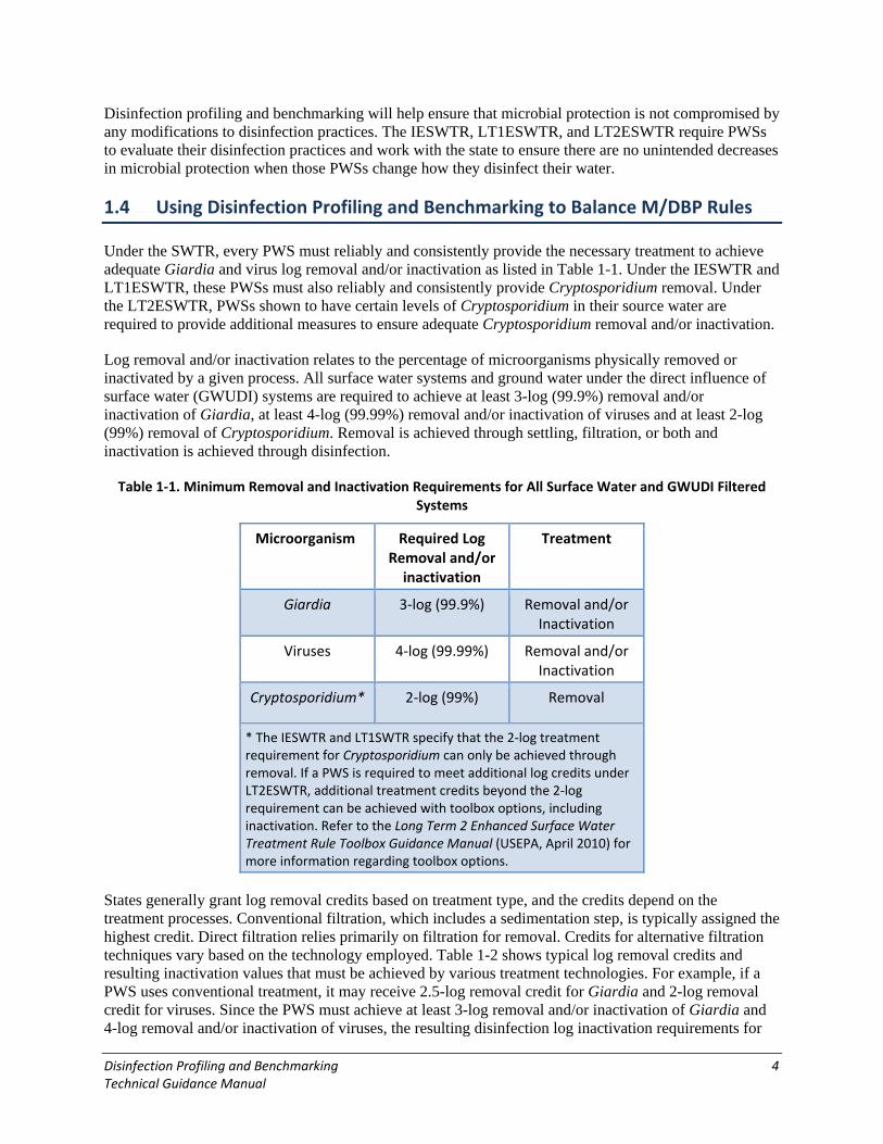
Under the SWTR, every PWS must reliably and consistently provide the necessary treatment to achieve adequate Giardia and virus log removal and/or inactivation as listed in Table 1-1. Under the IESWTR and LT1ESWTR, these PWSs must also reliably and consistently provide Cryptosporidium removal. Under the LT2ESWTR, PWSs shown to have certain levels of Cryptosporidium in their source water are required to provide additional measures to ensure adequate Cryptosporidium removal and/or inactivation.
Log removal and/or inactivation relates to the percentage of microorganisms physically removed or inactivated by a given process. All surface water systems and ground water under the direct influence of surface water (GWUDI) systems are required to achieve at least 3-log (99.9%) removal and/or inactivation of Giardia, at least 4-log (99.99%) removal and/or inactivation of viruses and at least 2-log (99%) removal of Cryptosporidium. Removal is achieved through settling, filtration, or both and inactivation is achieved through disinfection.
Table 1-1. Minimum Removal and Inactivation Requirements for All Surface Water and GWUDI Filtered Systems
Microorganism Required Log Removal and/or
inactivation
Treatment
Giardia 3-log (99.9%) Removal and/or Inactivation
Viruses 4-log (99.99%) Removal and/or Inactivation
Cryptosporidium* 2-log (99%) Removal
* The IESWTR and LT1SWTR specify that the 2-log treatment requirement for Cryptosporidium can only be achieved through removal. If a PWS is required to meet additional log credits under LT2ESWTR, additional treatment credits beyond the 2-log requirement can be achieved with toolbox options, including inactivation. Refer to the Long Term 2 Enhanced Surface Water Treatment Rule Toolbox Guidance Manual (USEPA, April 2010) for more information regarding toolbox options.
States generally grant log removal credits based on treatment type, and the credits depend on the treatment processes. Conventional filtration, which includes a sedimentation step, is typically assigned the highest credit. Direct filtration relies primarily on filtration for removal. Credits for alternative filtration techniques vary based on the technology employed. Table 1-2 shows typical log removal credits and resulting inactivation values that must be achieved by various treatment technologies. For example, if a PWS uses conventional treatment, it may receive 2.5-log removal credit for Giardia and 2-log removal credit for viruses. Since the PWS must achieve at least 3-log removal and/or inactivation of Giardia and 4-log removal and/or inactivation of viruses, the resulting disinfection log inactivation requirements for

Disinfection Profiling and Benchmarking 5 Technical Guidance Manual
Giardia and viruses are 0.5-log and 2-log, respectively. For unfiltered systems (i.e., systems that have received filtration avoidance determinations), 3-log inactivation of Giardia and 4-log inactivation of viruses can only be achieved using disinfection. PWSs should check with their state for specific removal credits and inactivation requirements in case they differ from those listed in Table 1-2.
Table 1-2. Typical Removal Credits and Inactivation Requirements for Various Treatment Technologies
Process
Log Removal and/or Inactivation Required
Typical Log Removal Credits
Resulting Disinfection Log
Inactivation Requirements
Giardia Viruses Giardia Viruses Giardia Viruses
Conventional Treatment 3.0 4.0 2.5 2.0 0.5 2.0
Direct Filtration 3.0 4.0 2.0 1.0 1.0 3.0
Slow Sand Filtration 3.0 4.0 2.0 2.0 1.0 2.0
Diatomaceous Earth Filtration 3.0 4.0 2.0 1.0 1.0 3.0
Alternative (membranes, bag filters, cartridges)
3.0 4.0 * * * *
Unfiltered 3.0 4.0 0 0 3.0 4.0
Source: USEPA. March 1991.
* PWSs must demonstrate to the state by pilot study or other means that the alternative filtration technology provides the minimum required log removal and inactivation shown in Table 1-1.
While minimum required levels of disinfection are regulated by the SWTR, the Stage 1 and Stage 2 DBPRs, herein referred to as “the DBPRs”, regulate the levels of DBPs allowed in distribution systems. The DBPs trihalomethanes and haloacetic acids are formed when organic matter in the water reacts with disinfectants such as chlorine. The MCLs of the regulated DBPs under the DBPRs are based on locational running annual averages (LRAAs) at or less than the following levels:
• Total Trihalomethanes (TTHM) at 0.080 milligrams per liter (mg/L); and • Haloacetic Acids Five (HAA5) at 0.060 milligrams per liter (mg/L).
The DBPRs also set maximum residual disinfectant levels (MRDLs) for chlorine, chloramines, and chlorine oxide.
In order to meet the TTHM and HAA5 MCL requirements of the DBPRs, PWSs may need to consider changing their disinfection practices. PWSs with high levels of DBPs may need to modify disinfection practices to reduce the formation of DBPs. Some of these changes, such as the use of lower concentrations of disinfectant, will lessen microbial inactivation and may produce water of unsatisfactory microbial quality. Likewise, some PWSs may make significant changes to their disinfection practices to provide additional treatment for Cryptosporidium under the LT2ESWTR. The disinfection profiling and benchmarking requirements under IESWTR and LT1ESWTR were defined to protect public health by assessing the risk of exposure to microbial pathogens as PWSs take steps to comply with the DBPR requirements. The LT2ESWTR includes disinfection profile and benchmark requirements to ensure that any significant change in disinfection, whether for DBP control under the DBPRs, improved Cryptosporidium control under the LT2ESWTR, or both, does not significantly compromise existing

Disinfection Profiling and Benchmarking 6 Technical Guidance Manual
Giardia and virus protection. The LT2ESWTR requires that PWSs and states evaluate the effects of significant changes in disinfection practice on current microbial treatment levels. Disinfection profiling and benchmarking serve as tools for making such evaluations.
Under the IESWTR, LT1ESWTR, and LT2ESWTR, the disinfection benchmark is not intended to function as a regulatory standard. Rather, the objective of the disinfection profiling and benchmarking requirements is to facilitate interactions between the state and PWS to assess the impacts of proposed changes on microbial protection. Disinfection profiling and benchmarking can help decision-makers identify the strengths and weaknesses of existing systems and choose appropriate system modifications (see Chapter 7).
Final decisions regarding levels of disinfection for Giardia and viruses, beyond the minimum required by federal regulations, will continue to be left to the states in consultation with PWSs. To ensure that the level of treatment for both protozoan and viral pathogens is appropriate, states and PWSs should also consider site-specific factors such as source water contamination levels and the reliability of treatment processes.
1.5 Overview of Disinfection Profiling and Benchmarking Requirements
As stated in Section 1.1, this revised guidance is based on disinfection profiling and benchmarking requirements under the LT2ESWTR. Prior to LT2ESWTR, PWSs were required to develop a profile for Giardia (and viruses if chloramines, ozone, or chlorine dioxide were used as the primary disinfectant2 or if required by the state) under the IESWTR or LT1ESWTR if they were a community water system (CWS) or a non-transient non-community water system (NTNCWS) that had a surface water or GWUDI source and had DBP levels in their distribution system exceeding the following conditions:
2 Primary disinfectant is defined as the disinfectant used in a treatment system to achieve the necessary microbial inactivation. Secondary disinfectant is defined as the disinfectant used in a treatment system to maintain the disinfectant residual throughout the distribution system.
• The TTHM annual average, based on quarterly samples, was greater than 0.064 mg/L; or • The HAA5 annual average, based on quarterly samples, was less than 0.048 mg/L.
The dates to complete a profile depended on a PWS’s size and ranged from March 2000 to January 2004. Only PWSs that were required to develop a disinfection profile and then subsequently proposed to make significant changes to their disinfection practices were required to develop a benchmark and submit it along with other pertinent information to the state.
Under the LT2ESWTR, any PWS that has a surface water or GWUDI source and plans to make a significant change to its disinfection practices must develop a disinfection profile and calculate a disinfection benchmark for Giardia and viruses. The EPA believes that profiling for both target pathogens (Giardia and viruses) is appropriate because the types of treatment changes that PWSs will make to comply with the LT2ESWTR could lead to a significant change in the inactivation level for one pathogen but not the other (USEPA, August 2007). Disinfection benchmarking ensures that PWSs maintain protection against microbial pathogens as they implement the DBPRs and LT2ESWTR.
In general, viruses are more sensitive to chlorine than Giardia and Cryptosporidium but are more resistant to ultraviolet (UV) light disinfection. A PWS that adds UV light disinfection to meet Cryptosporidium treatment requirements will maintain a high level of inactivation for Giardia and Cryptosporidium but, if
Disinfection Profiling and Benchmarking 7 Technical Guidance Manual
the addition of UV disinfection is coupled with a corresponding reduction in chlorination, the level of treatment for viruses may be significantly reduced.
PWSs are required to keep their disinfection profile and benchmark on file for review during sanitary surveys. Also, PWSs must notify the state as described in Section 1.3 before making significant changes to their disinfection practices.
The flowchart in Figure 1-3 provides information on the LT2ESWTR disinfection profiling and benchmarking requirements.

Disinfection Profiling and Benchmarking 8 Technical Guidance Manual
Figure 1-3. LT2ESWTR Disinfection Profile and Benchmark Decision Tree
Are you a public water system (PWS) that uses surface water or
ground water under the direct influence of surface water?
No disinfection profiling or benchmarking is required
under the LT2ESWTR provisions.
NO
YES
Do you plan to make any of the following significant
changes to your disinfection practices? • Change to the point of disinfection;
• Change to the disinfectant(s) used in the treatment plant; • Change to the disinfection process
3; or
• Any other modification identified by your primacy agency as a significant change
to your disinfection practice.
YES
Did your PWS develop a disinfection profile previously and
keep it on file? NO
Your PWS must develop disinfection profiles for
Giardia lamblia and viruses. YES
Has your PWS made a significant change to its
treatment practice or changed sources since the data for the
earlier disinfection profile were collected?
YES
NO
NO
Does the existing profile include a disinfection profile for
Giardia lamblia and a disinfection profile for viruses?
NO
YES
Your PWS must develop a virus disinfection profile using the
same monitoring data on which the Giardia lamblia
profile is based.
Prior to changing the disinfection practice, your PWS must
notify its primacy agency and must include in this notice the following information:
• A completed disinfection profile and disinfection benchmark for Giardia lamblia and viruses;
• A description of the proposed change in disinfection practice; and
• An analysis of how the proposed change will affect the current level of disinfection.
Did your PWS do this?
THEN
YES
Your PWS is in compliance with the disinfection
profiling and benchmarking requirements.
Treatment technique violation.
NO
Use the information from the disinfection profiles to calculate the
log inactivation ratios and disinfection benchmarks for Giardia
lamblia and viruses.4
THEN
THEN
3Some modifications to the disinfection process may include changing the contact basin geometry and baffling conditions, changing the pH during disinfection, decreasing the disinfectant dose during warmer temperatures, and increasing or decreasing flow through the plant. 4The total inactivation ratio for Giardia must be calculated using the procedures specified in 40 CFR 141.709(d)(1) through (3). The log of inactivation for viruses must use a
protocol approved by the primacy agency.
Disinfection Profiling and Benchmarking 9 Technical Guidance Manual
1.6 Contents of this Guidance Document
This document is organized in the following chapters and appendices:
• Chapter 1 – Introduction
• Chapter 2 – Disinfection Segment
This chapter defines the term disinfection segment and describes ways in which a PWS can identify their disinfection segment(s).
• Chapter 3 – Data Collection
This chapter presents the data collection requirements for creating a disinfection profile.
• Chapter 4 – Calculating CT
This chapter presents methods and examples for calculating CT.
• Chapter 5 – Calculating Inactivation
This chapter presents information and examples for calculating Giardia and virus inactivation values to be used in the development of a disinfection profile.
• Chapter 6 – Developing the Disinfection Profile and Benchmark
This chapter provides information for developing a disinfection profile using calculated inactivation values. The chapter also presents information on when and how the disinfection benchmark must be calculated.
• Chapter 7 – Evaluating Disinfection Practice Modifications
This chapter discusses issues associated with making significant changes to treatment and how the disinfection profile and benchmark can be used to assess system modifications that may be considered for compliance.
• Chapter 8 – Treatment Considerations
This chapter gives an overview of different treatment methods and strategies PWSs can choose from when considering system modifications. This chapter also includes case studies on experiences with implementing different treatment methods.
• Appendix A – Glossary • Appendix B – CT Tables • Appendix C – Blank Worksheets • Appendix D – Examples • Appendix E – Tracer Studies • Appendix F – Calculating the Volume of each Sub-unit • Appendix G – Baffling Factors • Appendix H – Conservative Estimate, Interpolation, and Regression Method Examples

Disinfection Profiling and Benchmarking 10 Technical Guidance Manual
1.7 References
USEPA. August 2007. The Long Term 2 Enhanced Surface Water Treatment Rule (LT2ESWTR) Implementation Guidance. Washington, D.C. USEPA. April 2010. Long Term 2 Enhanced Surface Water Treatment Rule Toolbox Guidance Manual. EPA 815-R-09-016. Washington, D.C.

Disinfection Profiling and Benchmarking 11 Technical Guidance Manual
Chapter 2 — Disinfection Segment
2.1 Introduction
The first step in developing a disinfection profile is to identify the disinfection segments within the treatment plant. A disinfection segment is a section of a treatment system beginning at one disinfectant injection or monitoring point and ending at the next disinfectant injection or monitoring point referred to as the ‘residual sampling point’. Each disinfectant injection point in a system must be associated with at least one sampling point. Each segment begins at the point of disinfection application and ends at the disinfectant residual sampling point. This sampling point is located just prior to the next disinfection application point or, for the last disinfection segment, at or before the entrance to the distribution system or the first customer. Data collection takes place at the residual sampling points (see Chapter 3 for types of data collected).
2.2 Identifying Disinfection Segments
The suggested starting point for analyzing a plant is to develop a summary of the unit processes, disinfectant injection points, and monitoring points. It may be helpful to use a sketch or plan drawing of the plant, such as those shown in Figures 2-1 through 2-6, when defining disinfection segments. The number of disinfection segments within a treatment train must equal or exceed the number of disinfectant application points in the system. For plants with multiple points of disinfectant application, such as ozone followed by chlorine, or chlorine applied at several points in the treatment train, the treatment train should be divided into multiple disinfection segments. If a PWS has multiple treatment plants, a disinfection profile applies only to the treatment plant where the data were collected to develop the disinfection profile; (i.e., a disinfection profile is specific to a treatment plant). A PWS with multiple treatment plants and a common distribution system that makes a disinfectant change at one of the treatment plants should consider whether that change will impact water quality in the distribution system and whether other treatment adjustments (e.g., corrosion control) may need to be made at other plants.
Disinfection segments may include one or more unit processes of the treatment train. PWSs may treat the entire plant as one disinfection segment or they may find it useful to divide the plant into multiple segments based on different mixing conditions or treatment units. For example, in a direct filtration plant where chlorine is applied at the rapid mixing stage and free chlorine residual is measured at the entrance to the distribution system, the whole plant is a single disinfection segment. The chlorine residual that is measured at the entry point to the distribution system, however, will be lower than the chlorine residual at points upstream in the treatment train due to chlorine demand and decay at various treatment stages. As a result, using only the entry point chlorine residual measurement to calculate inactivation will give a conservative CT value for the plant. Measuring free chlorine residual at the end of each treatment unit may provide a higher (and more representative) CT value (see Chapter 4 and Chapter 5 for a discussion on the relationship between CT and log inactivation).
Each treatment train will have its own disinfection profile based on its disinfection segment(s). Therefore, plants with multiple treatment trains may have multiple disinfection profiles. If the treatment trains are identical, and flow is split equally, the disinfection segments and corresponding profile for each train should be the same. If the treatment trains are very different, the PWS should identify all disinfection segments in each train and develop a disinfection profile for each train separately.

Disinfection Profiling and Benchmarking 12 Technical Guidance Manual
2.2.1 Single Disinfection Segment
Figure 2-1 shows a simple plant, with one injection point and one monitoring point, resulting in a single disinfection segment. The disinfection segment begins at the chlorine injection point prior to the clearwell and ends at the monitoring point after the clearwell.
Figure 2-1. Plant Schematic Showing a Conventional Filtration Plant with One Disinfection Segment
DistributionSystem
Sedimentation
ChlorineInjected
FiltrationClearwell
Monitoring PointCl2 ResidualTemperature
pH
One Disinfection Segment:One injection point, one monitoring point
Intake
FlocculationCoagulation
2.2.2 Multiple Disinfection Segments
Figure 2-2 is an example of a plant with two injection points and two monitoring points, resulting in two disinfection segments. Disinfection Segment 1 starts at the chlorine injection point prior to the coagulation basin and ends at the monitoring point after the filters. Disinfection Segment 2 starts at the chlorine injection point between the filters and the clearwell, and ends at the monitoring point after the clearwell and prior to the first customer.
Even for this simple plant, the analysis of how much disinfection takes place in the plant may be complicated. In this example, disinfection occurs in the coagulation basin, flocculation basin, sedimentation basin, filters, and clearwell, as well as in all the associated piping. PWSs may choose to break Disinfection Segment 1 into further segments adding chlorine residual monitoring points at the end of each of the treatment units.

Disinfection Profiling and Benchmarking 13 Technical Guidance Manual
Figure 2-2. Plant Schematic Showing a Conventional Filtration Plant with Two Disinfection Segments
DistributionSystem
Sedimentation
ChlorineInjected
Coagulation
Clearwell
Disinfection Segment 2Monitoring Point
Cl2 ResidualTemperature
pH
Intake
Chlorine Injected
Disinfection Segment 1Monitoring Point
Cl2 ResidualTemperature
pH
Disinfection Segment 2
Disinfection Segment 1
Filtration
Flocculation
Figure 2-3 is an example of a plant with one injection point and multiple monitoring points. Although the PWS is required to have a minimum of one monitoring point, the chlorine is sampled in four locations to make use of the higher chlorine residual values at some segments in the plant; this results in a higher CT value for SWTR compliance, as opposed to monitoring at one location after the clearwell where the chlorine residual will be much lower than measurements prior to the clearwell. The first disinfection segment starts at the chlorine injection point before coagulation and ends at the first monitoring point after coagulation. The next three disinfection segments begin at one monitoring point and end at the following monitoring point. Therefore, even though there is only one injection point in this plant, there are four disinfection segments.

Disinfection Profiling and Benchmarking 14 Technical Guidance Manual
Figure 2-3. Plant Schematic Showing One Injection Point with Multiple Disinfection Segments
DistributionSystem
Sedimentation
ChlorineInjected
Coagulation
Clearwell
Disinfection Segment 4 Monitoring Point
Cl2 ResidualTemperature
pH
Intake
Disinfection Segment 3
Disinfection Segment 1
Disinfection Segment 2
Disinfection Segment 2Monitoring Point
Cl2 ResidualTemperature
pH
Disinfection Segment 1Monitoring Point
Cl2 ResidualTemperature
pH
Filtration
Disinfection Segment 4
Disinfection Segment 3Monitoring Point
Cl2 ResidualTemperature
pH
Flocculation
Figure 2-4 is another example of a more complicated plant schematic. Similar to Figure 2-3, this plant has four disinfection segments. The difference between these two plants is that the PWS in Figure 2-4 injects ammonia prior to the clearwell to form chloramines. The use of a different disinfectant results in a distinct disinfection segment.
Figure 2-4. Plant Schematic Showing Two Injection Points with Multiple Disinfection Segments
DistributionSystem
Sedimentation
ChlorineInjected
Coagulation
Clearwell
Disinfection Segment 4 Monitoring Point
Chloramine ResidualTemperature
Intake
Ammonia Injected
Disinfection Segment 3Disinfection Segment 1
Disinfection Segment 2
Disinfection Segment 2Monitoring Point
Cl2 ResidualTemperature
pH
Disinfection Segment 1Monitoring Point
Cl2 ResidualTemperature
pH
Filtration
Disinfection Segment 4
Disinfection Segment 3Monitoring Point
Cl2 ResidualTemperature
pH
Flocculation

Disinfection Profiling and Benchmarking 15 Technical Guidance Manual
2.2.3 Disinfection Segments for Multiple Treatment Trains
For some system configurations, one profile would not accurately characterize the entire treatment process. In these cases, multiple profiles are suggested. Figure 2-5 shows a plant with multiple treatment trains and multiple disinfection segments. In this example, the treatment trains are identical in that all unit processes in both trains have the same dimensions, operating rates, and hydraulic capacities. Since the treatment trains are identical, and flow is split equally between the treatment trains, the disinfection profiles for Disinfection Segments 1a and 1b should be identical. Similarly, the disinfection profiles for Disinfection Segments 2a and 2b should be identical. However, PWSs should check with the state to determine if separate disinfection profiles are required for each treatment train.
Figure 2-5. Plant Schematic Showing Two Identical Treatment Trains and Each with Multiple Disinfection Segments
DistributionSystem
Sedimentation
ChlorineInjected
Coagulation
Clearwell
Disinfection Segment 2bMonitoring Point
Cl2 ResidualTemperature
pH
Intake
Chlorine Injected
Disinfection Segment 1bMonitoring Point
Cl2 ResidualTemperature
pH
Disinfection Segment 2b
Disinfection Segment 1b
Filtration
Flocculation
Disinfection Segment 1aMonitoring Point
Cl2 ResidualTemperature
pH
Disinfection Segment 2aMonitoring Point
Cl2 ResidualTemperature
pH
Disinfection Segment 2aDisinfection Segment 1a
Sedimentation
Coagulation
Clearwell
Chlorine Injected
Filtration
Flocculation
ChlorineInjected
DistributionSystem
1/2 of Flow
1/2 of Flow
FlowController*
*Note: Flow is split equally between treatment trains.
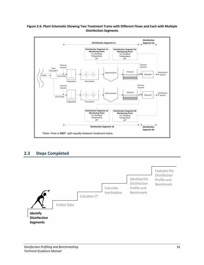
Figure 2-6 shows a plant with two treatment trains and multiple disinfection segments. In this example, although the treatment trains are identical the flow is not split equally between the treatment trains. The disinfection profiles for Disinfection Segments 1a and 1b may not be identical. Similarly, the disinfection profiles for Disinfection Segments 2a and 2b may not be identical. Therefore, this plant should develop a separate disinfection profile for each treatment train. Again, the PWS should check with the state on this issue.
Disinfection Profiling and Benchmarking 16 Technical Guidance Manual
Figure 2-6. Plant Schematic Showing Two Treatment Trains with Different Flows and Each with Multiple Disinfection Segments
DistributioSystem
Sedimentation
ChlorineInjected
Coagulation
Clearwell
Disinfection Segment 2bMonitoring Point
Cl2 ResidualTemperature
pH
Disinfection Segment 2b
Disinfection Segment 1b
*Note: Flow is NOT split equally between treatment trains.
Intake
Chlorine Injected
Disinfection Segment 1bMonitoring Point
Cl2 ResidualTemperature
pH
Filtration
Flocculation
Disinfection Segment 1aMonitoring Point
Cl2 ResidualTemperature
pH
Disinfection Segment 2aMonitoring Point
Cl2 ResidualTemperature
pH
Disinfection Segment 2aDisinfection Segment 1a
Sedimentation
Coagulation
Clearwell
Chlorine Injected
Filtration
Flocculation
ChlorineInjected
DistributioSystem
2/3 of Flow
1/3 of Flow
FlowController*
n
n
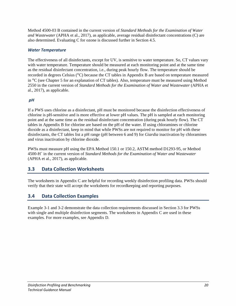
2.3 Steps Completed
Identify Disinfection Segments
Collect Data
Calculate CT
Calculate Inactivation
Develop the Disinfection Profile and Benchmark
Evaluate the
Profile and Benchmark
Disinfection

Disinfection Profiling and Benchmarking 17 Technical Guidance Manual
2.4 Next Step
Upon completing the activities in this chapter, the PWS will have completed the first of six steps in disinfection profiling: identifying disinfection segments. After all of the disinfection segments in the treatment system have been identified, data must be collected for each disinfection segment, as described in Chapter 3.

Disinfection Profiling and Benchmarking 18 Technical Guidance Manual
Chapter 3 — Data Collection
3.1 Introduction
Once a PWS has identified each disinfection segment, it must collect operational data during peak-hour flows for each segment for a minimum of 12 consecutive months. The data required to create a disinfection profile and benchmark are described in this section. PWSs required to comply with the disinfection profiling requirements of the IESWTR were required to collect daily measurements, while PWSs complying with the disinfection profiling requirements of the LT1ESWTR were required to collect weekly measurements of operational data. To develop a disinfection profile for the LT2ESWTR, a PWS must collect data at least once per week on the same day of the week for one year (52 measurements), during peak hourly flow for that day. PWSs may collect and use additional data to develop their disinfection profiles, as long as the data are evenly spaced over time.
3.2 Use of Grandfathered Data
PWSs can meet the disinfection profiling requirements under the LT2ESWTR by using previously collected data (i.e., grandfathered data). Use of grandfathered data is allowed if the PWS has not made a significant change in its disinfection practice or changed sources since the data were collected. This will permit most PWSs that prepared a disinfection profile under the IESWTR or the LT1ESWTR to avoid collecting any new operational data for developing a profile under the LT2ESWTR. PWSs that produced a disinfection profile for Giardia but not viruses under the IESWTR or LT1ESWTR must also develop the disinfection profile for viruses under the LT2ESWTR using the same monitoring data on which the original Giardia profile was based.
3.2.1 Data Needed for the Disinfection Profile
The basic data requirements for creating profiles based on Giardia and viruses are the same. Therefore, if a utility collects operating data sufficient to profile for Giardia, it can also develop a profile for viruses using the same data, as described in Chapter 5. Data can be measured manually or with on-line instrumentation as available. Data must be collected at least weekly for a period of twelve consecutive months. The following data must be gathered at peak hourly flow at the disinfectant residual sampling points for each disinfection segment in the treatment plant:
• Peak Hourly Flow (Q). • Residual Disinfectant Concentration (C). • Water Temperature. • pH (if chlorine is used).
Data collected must be representative of the entire treatment plant. PWSs should consider adding or removing disinfection segments and residual sampling points to ensure that data sufficiently characterize system performance.
Peak Hourly Flow Rate (Q)
The time that the disinfectant is in contact with water in the disinfection segment, referred to as contact time (T) must be determined to calculate the CT value. Contact time is a function of flow. When the flow increases, the time the water spends in the plant and in contact with the disinfectant decreases. Using the peak hourly flow for analysis provides a conservative value for contact time. Therefore, all operational

Disinfection Profiling and Benchmarking 19 Technical Guidance Manual
data that affect the CT value are measured at peak hourly flow. Some PWSs may be able to use a single peak hourly flow for the entire plant. In other PWSs with multiple treatment trains, or where the peak hourly flow varies between disinfection segments, each treatment train or disinfection segment must be sampled during that segment’s peak hourly flow. For example, the flow rate after the clearwell will be driven by the finished water pumps whereas the flowrate through the plant is driven by the raw water pumping rate or gravity flow.
Some options for determining peak hourly flow are:
• Flow meter records. • Design flow rate. • Maximum loading rates to the filters or other treatment process units. • Raw water pumps records. • Historical maximum flow.
When determining peak hourly flow, PWSs may want to take into consideration the location of their disinfection segment. For example, a PWS with a single disinfection segment with disinfection prior to the clearwell may consider using clearwell pumping rates versus raw water pump records to determine the peak hourly flow rate.
PWSs with supervisory control and data acquisition (SCADA) systems will be able to review records, identify the peak hourly flow and then obtain the residual disinfectant concentration, temperature, and pH (if chlorine is used) that were recorded during peak hourly flow. PWSs without SCADA should coordinate with the state to develop a procedure that allows the PWS to best identify peak hourly flow for data collection.
One possible approach for PWSs without SCADA is to determine when peak hourly flow occurred the day before data must be collected. The PWS can collect the residual disinfectant concentration, temperature, and pH (if chlorine is used) on the required day at the same time that peak hourly flow occurred on the previous day. Alternatively, PWSs may collect residual disinfectant concentration, temperature, and pH (if chlorine is used) data at three different times (such as before, during, and after) near the time when peak hourly flow occurred on the previous day. Then, based on pump records or other information, PWSs can determine when peak hourly flow actually occurred and use the data that were collected nearest to the time of peak hourly flow.
Residual Disinfectant Concentration (C)
The disinfectant residual concentration (C) is defined as the concentration of disinfectant measured in mg/L in a representative sample of water (40 CFR 141.2). This residual is measured at the residual sampling point in each disinfection segment. If, for example, a treatment plant has three disinfection segments, it will have three residual sampling points where data must be measured. The residual disinfectant concentration is monitored for each disinfection segment during peak hourly flow and is measured in milligrams per liter (mg/L). Monitoring the residual disinfectant at more than one location results in higher CT values because residual disinfectant concentration decreases with each subsequent treatment process. For more information on CT refer to Chapter 4.
The residual disinfectant concentration must be measured using methods listed in the current version of Standard Methods for the Examination of Water and Wastewater (APHA et al., 2017), as applicable. If approved by the state, residual disinfectant concentrations for free chlorine and combined chlorine may be measured using DPD (N, N-diethyl-p-phenylenediamine) colorimetric test kits (40 CFR 141.74). There are additional considerations for PWSs using ozone. While ozone residual values are measured using
Disinfection Profiling and Benchmarking 20 Technical Guidance Manual
Method 4500-03 B contained in the current version of Standard Methods for the Examination of Water and Wastewater (APHA et al., 2017), as applicable, average residual disinfectant concentrations (C) are also determined. Evaluating C for ozone is discussed further in Section 4.5.
Water Temperature
The effectiveness of all disinfectants, except for UV, is sensitive to water temperature. So, CT values vary with water temperature. Temperature should be measured at each monitoring point and at the same time as the residual disinfectant concentration, i.e., during peak hourly flow. The temperature should be recorded in degrees Celsius (°C) because the CT tables in Appendix B are based on temperature measured in °C (see Chapter 5 for an explanation of CT tables). Also, temperature must be measured using Method 2550 in the current version of Standard Methods for the Examination of Water and Wastewater (APHA et al., 2017), as applicable.
pH
If a PWS uses chlorine as a disinfectant, pH must be monitored because the disinfection effectiveness of chlorine is pH-sensitive and is more effective at lower pH values. The pH is sampled at each monitoring point and at the same time as the residual disinfectant concentration (during peak hourly flow). The CT tables in Appendix B for chlorine are based on the pH of the water. If using chloramines or chlorine dioxide as a disinfectant, keep in mind that while PWSs are not required to monitor for pH with these disinfectants, the CT tables list a pH range (pH between 6 and 9) for Giardia inactivation by chloramines and virus inactivation by chlorine dioxide.
PWSs must measure pH using the EPA Method 150.1 or 150.2, ASTM method D1293-95, or Method 4500-H+ in the current version of Standard Methods for the Examination of Water and Wastewater (APHA et al., 2017), as applicable.
3.3 Data Collection Worksheets
The worksheets in Appendix C are helpful for recording weekly disinfection profiling data. PWSs should verify that their state will accept the worksheets for recordkeeping and reporting purposes.
3.4 Data Collection Examples
Example 3-1 and 3-2 demonstrate the data collection requirements discussed in Section 3.3 for PWSs with single and multiple disinfection segments. The worksheets in Appendix C are used in these examples. For more examples, see Appendix D.
Disinfection Profiling and Benchmarking 21 Technical Guidance Manual
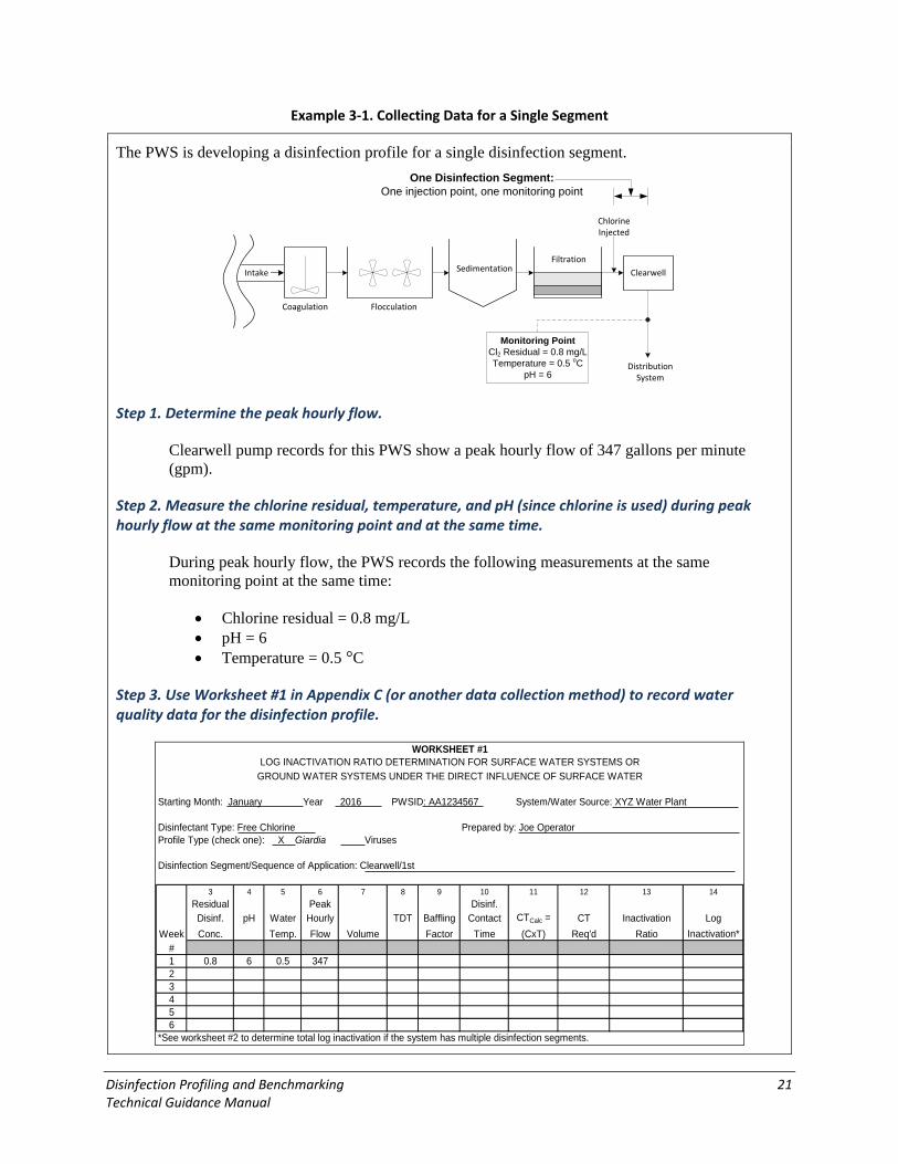
Example 3-1. Collecting Data for a Single Segment
The PWS is developing a disinfection profile for a single disinfection segment.
DistributionSystem
Sedimentation
Coagulation
FiltrationClearwell
Monitoring PointCl2 Residual = 0.8 mg/LTemperature = 0.5 oC
pH = 6
One injection point, one monitoring point
Intake
ChlorineInjected
Flocculation
One Disinfection Segment:
Step 1. Determine the peak hourly flow.
Clearwell pump records for this PWS show a peak hourly flow of 347 gallons per minute (gpm).
Step 2. Measure the chlorine residual, temperature, and pH (since chlorine is used) during peak hourly flow at the same monitoring point and at the same time.
During peak hourly flow, the PWS records the following measurements at the same monitoring point at the same time:
• Chlorine residual = 0.8 mg/L • pH = 6 • Temperature = 0.5 °C
Step 3. Use Worksheet #1 in Appendix C (or another data collection method) to record water quality data for the disinfection profile.
WORKSHEET #1LOG INACTIVATION RATIO DETERMINATION FOR SURFACE WATER SYSTEMS OR
GROUND WATER SYSTEMS UNDER THE DIRECT INFLUENCE OF SURFACE WATER
Starting Month: January Year 2016 PWSID: AA1234567 System/Water Source: XYZ Water Plant
Disinfectant Type: Free Chlorine Prepared by: Joe OperatorProfile Type (check one): X Giardia Viruses
Disinfection Segment/Sequence of Application: Clearwell/1st
3 4 5 6 7 8 9 10 11 12 13 14Residual Peak Disinf.Disinf. pH Water Hourly TDT Baffling Contact CTCalc = CT Inactivation Log
Week Conc. Temp. Flow Volume Factor Time (CxT) Req'd Ratio Inactivation*# C (mg/L) (oC) (gpm) (gal) (min.) T (min.) (min-mg/L) (min-mg/L) (Col 11 / Col 12)1 0.8 6 0.5 34723456
*See worksheet #2 to determine total log inactivation if the system has multiple disinfection segments.

Disinfection Profiling and Benchmarking 22 Technical Guidance Manual
Example 3-2. Collecting Data for Multiple Disinfection Segments
The PWS is developing a disinfection profile for multiple disinfection segments.
DistributionSystem
Sedimentation
ChlorineInjected
Coagulation
Clearwell
Disinfection Segment 4 Monitoring Point
Cl2 Residual = 0.8 mg/LTemperature = 5 oC
pH = 7.5
Intake
Disinfection Segment 3
Disinfection Segment 1
Disinfection Segment 2
Disinfection Segment 2Monitoring Point
Cl2 Residual = 0.7 mg/LTemperature = 5 oC
pH = 7.5
Disinfection Segment 1Monitoring Point
Cl2 Residual = 1.0 mg/LTemperature = 5 oC
pH = 7.5
Filtration
Disinfection Segment 4
Disinfection Segment 3Monitoring Point
Cl2 Residual = 0.3 mg/LTemperature = 5 oC
pH = 7.5
Chlorine Injected
Step 1. Determine the peak hourly flow for Disinfection Segments 1 through 4.
From the raw water pump records, the PWS determines the peak hourly flow to be 347 gpm for Disinfection Segments 1, 2, and 3.
From the clearwell pump records, the PWS determines the peak hourly flow to be 370 gpm for Disinfection Segment 4.
Step 2. Measure the chlorine residual, temperature, and pH (since chlorine is used) during peak hourly flow at the same monitoring point and at the same time.
During peak hourly flow, the PWS records the following measurements at the same monitoring point at the same time:
Disinfection Segment
Chlorine Residual (mg/L)
Temperature (°C) pH
1 1.0 5 7.5 2 0.7 5 7.5 3 0.3 5 7.5 4 0.8 5 7.5
Step 3. Use Worksheet #1 in Appendix C (or another data collection method) to record water quality data for the disinfection profile.
For PWSs with multiple segments, a separate copy of Worksheet #1 should be used for each disinfection segment. Example D-2 in Appendix D illustrates how to complete Worksheet #1 for multiple disinfection segments.

Disinfection Profiling and Benchmarking 23 Technical Guidance Manual
3.5 Steps Completed
Identify Disinfection
Collect Data
Calculate CT
Calculate Inactivation
Develop the Disinfection Profile and Benchmark
Evaluate the Disinfection Profile and Benchmark
Segments
3.6 Next Step
Upon completing the activities in this chapter, the PWS will have completed the second of six steps: collecting data. Now the CT value can be calculated. Chapter 4 explains how to calculate CT.
3.7 References
APHA, AWWA, WEF. 2017. Standard Methods for the Examination of Water and Wastewater, 23rd Edition. APHA, Washington, D.C.

Disinfection Profiling and Benchmarking 24 Technical Guidance Manual
Chapter 4 — Calculating CT
4.1 Introduction
The CT method is used to evaluate the amount of disinfection a treatment plant achieves and to determine compliance with the SWTR. If a PWS is required to complete a disinfection profile for the IESWTR, LT1ESWTR, or LT2ESWTR, it must collect operational data (or use grandfathered data) and calculate the CT value for each disinfection segment, known as CTcalc. The CTcalc value derived for each disinfection segment will be used to calculate the inactivation ratio for each disinfection segment. This section provides an overview of the procedure to determine C and T to calculate CTcalc values. For PWSs that use ozone as a disinfectant, refer to Section 4.5 for the applicable method for calculating CT.
The CT method cannot be used to evaluate UV disinfection. For PWSs that use UV light for disinfection, unlike chemical disinfectants, UV light does not leave a chemical residual that can be monitored to determine UV dose and inactivation credit. The UV dose depends on the UV intensity (measured by UV sensors), the flow rate, and the UV absorbance. The EPA’s Ultraviolet Disinfection Guidance Manual for the Final Long Term 2 Enhanced Surface Water Treatment Rule (UVDGM) (USEPA, November 2006) provides guidance to PWSs using UV light for disinfection.
4.2 What is CT?
CT simply stands for the product of concentration (C) and contact time (T). Conceptually, the CT value is a measure of disinfection effectiveness for the time that the water and disinfectant are in contact. It is evaluated as the product of disinfectant residual concentration and the contact time as shown in Equation 4-1. “C” is the disinfectant residual concentration measured in mg/L at peak hourly flow and “T” is the time, measured in minutes that the disinfectant is in contact with the water at peak hourly flow. The contact time (T) is measured from the point of disinfectant injection to a point where the residual is measured. From Equation 4-1, it can be seen that any design modifications that can increase T may allow the same inactivation (CT) with a decreased disinfectant residual. The CTcalc is the calculated CT value for a system based on its actual performance. Section 5.3 will discuss CT required, which is the required CT value that a PWS must achieve to be in compliance.
Equation 4-1
CTcalc (minutes-mg/L) = C x T
C = Residual disinfectant concentration measured during peak hourly flow in mg/L. T = Time, measured in minutes, that the water is in contact with the disinfectant.
4.3 Determining “C”
“C” is the residual disinfectant concentration measured during peak hourly flow in mg/L. The residual disinfectant concentration must be measured for each disinfection segment. In addition, the residual disinfectant concentration must be measured at least once per week during peak hourly flow (if using grandfathered data collected for compliance with IESWTR profiling requirements, PWSs will have daily measurements during peak hourly flow). See Chapter 3 for information on the residual disinfectant concentration.

Disinfection Profiling and Benchmarking 25 Technical Guidance Manual
4.4 Determining “T”
Water does not flow through all treatment processes in a perfectly mixed condition. In some treatment units there can be substantial short circuiting. The disinfectant contact time (T), also referred to as T10 in the Guidance Manual for Compliance with the Filtration and Disinfection Requirements for Public Water Systems Using Surface Water (USEPA, March 1991), is an estimate of the detention time within a basin or treatment unit during which 90 percent of the water passing through the unit is retained within the basin or treatment unit. T can be determined experimentally through a tracer study or it can be estimated based on a theoretical detention time (TDT) and baffling factor (BF). Appendix E provides a detailed discussion of tracer studies and how they can be used to determine disinfectant contact time. Estimation of T based on theoretical analysis is discussed here.
Once the peak hourly flow in each disinfection segment has been determined as described in Chapter 3, the following steps may be used to calculate T for a treatment system:
• For each basin, pipe, or unit process in each disinfection segment, calculate:
o Volume (V) (see Section 4.4.1).
o Theoretical detention time (TDT) (see Section 4.4.2).
o Baffling factor (BF) (see Section 4.4.3).
o Contact time (T) for each basin, pipe, or unit process based on TDT and BF (see Section 4.4.4).
• Sum the T values for each basin, pipe, or unit process to obtain the total contact time (T) for the disinfection segment.
4.4.1 Volume
The volume of water contained in each basin, pipe, or unit process in a disinfection segment is used to calculate T for that segment. Since some treatment units, such as clearwells, can have fluctuating levels that affect volume, PWSs should consult with the state regarding what volume should be used for the disinfection profile. Using internal volumes for units to account for wall thicknesses when possible can provide a more accurate estimate of the water volume. PWSs and states may want to consider the following options:
• Volumes can be based on the minimum volume that can occur in the treatment unit. This approach is the most conservative.
• Volumes can be based on the actual volume realized in the treatment unit during peak hourly flow if adequate information is available to identify the actual volume.
• Volumes can be based on the lowest volume realized in the treatment unit for that day.
Table 4-1 provides equations used to find the volume of the specific sub-units or segments. See Appendix F for detailed examples of sub-units and volume equations.

Disinfection Profiling and Benchmarking 26 Technical Guidance Manual
Table 4-1. Volume Equations for Shapes
Shape Example of Unit with This Shape Volume Equation
Cylindrical Pipes Raw Water Pipe, Plant Piping, Finished Water Pipe Length x Cross-sectional Area (πr2)
Rectangular Basins
Rapid Mix, Flocculation and Sedimentation Basins, Clearwells
Length x Width x Minimum Water Depth
Cylindrical Basins Rapid Mix, Flocculation and Sedimentation Basins, Clearwells
Minimum Water Depth x Cross-sectional Area (πr2)
Rectangular Filters
Filtration Surface Area of Filter x Depth of Water Above Filter Surface (Vol. of water in the media pores may also be used by calculating Length x Width x Media Depth x Percent Pore Space.)
4.4.2 Theoretical Detention Time
The theoretical detention time (TDT) is the theoretical time that the water is in a basin, pipe, or unit process assuming perfect plug flow. Perfect plug flow assumes no short-circuiting within the basin, pipe, or unit process and all the water follows a single flow path. The TDT is calculated by dividing the volume based on low water level by the peak hourly flow (Equation 4-2).
Equation 4-2
TDT = V / Q
TDT = Theoretical Detention Time, in minutes V = Volume based on low water level, in gallons (gal) Q = Peak hourly flow, in gpm
4.4.3 Baffling Factor
The T in each basin, pipe, or unit process is a function of the physical configuration and baffling. The flow through a pipe is very different than the flow through an unbaffled basin (see Figure 4-1). The longest path a particle can take through a pipeline does not vary substantially from the shortest path. In the case of an unbaffled basin, however, some percentage of the flow may follow a path that goes directly from the inlet to the outlet. As a result, short-circuiting occurs and microorganisms in this path will only be in contact with the disinfectant for a relatively short time.

Disinfection Profiling and Benchmarking 27 Technical Guidance Manual
Figure 4-1. Baffling Characteristics of a Pipe and Clearwell
Baffling Factor = 1.0
Baffling Factor = 0.1
Top: This pipe demonstrates a plug flow condition in which all of the material sent througthe pipe discharges at the theoretical detention time (TDT) of the pipe. Bottom: This unbaffled basin demonstrates short-circuiting in which some of the material entering the basin would come out almost immediately, while other material that enters at the same time will be detained for a longer period of time. Short-circuiting occurs in basins with poor baffling.
h
Baffling factors (BFs) help estimate the contact time of a basin, pipe, or unit process based on the volume of and flow rate through the basin, pipe, or unit process. Baffling factors recommended in Table 4.2 were developed based on tracer studies of basins with varying sizes and configurations. Table 4-2 and Appendix G provide a summary of theoretical baffling factors for various baffling conditions and basins.
Table 4-2. Baffling Factors
Baffling Condition Baffling Factor
Baffling Description
Unbaffled (mixed flow)
0.1 None, agitated basin, very low length to width ratio, high inlet and outlet flow velocities.
Poor 0.3 Single or multiple unbaffled inlets and outlets, no intra-basin baffles.
Average 0.5 Baffled inlet or outlet with some intra-basin baffles.
Superior 0.7 Perforated inlet baffle, serpentine or perforated intra-basin baffles, outlet weir, or perforated launders.
Perfect (plug flow)
1.0 Very high length to width ratio (pipeline flow), perforated inlet, outlet and intra-basin baffles.
Source: USEPA. March 1991.

Disinfection Profiling and Benchmarking 28 Technical Guidance Manual
4.4.4 Calculate Contact Time
T in each basin, pipe, or unit process can be calculated once the TDT and BF are known (Equation 4-3). To evaluate total contact time in a disinfection segment, the T values for each basin, pipe and/or unit process within the segment have to be added together. Example 4-1 shows the procedure for determining T for a disinfection segment with only one clearwell. For examples with multiple units and segments, see Appendix D.
Equation 4-3
T = TDT x BF
T = Time, measured in minutes, that the water is in contact with the disinfectant. TDT = Theoretical detention time, in minutes BF = Baffling factor
Example 4-1. Determining “T” for a clearwell with no baffling
Peak HourlyFlow = 347 gpm
Residual MonitoringPoint
ChlorineInjected
ToDistribution
System
Side View
Minimum Operating Level
Diameter = 40 ft
Depth = 30 ft
ToDistribution
SystemPeak HourlyFlow = 347 gpm
Top View

Disinfection Profiling and Benchmarking 29 Technical Guidance Manual
Step 1. Measure the physical dimensions of the clearwell.
Measure the inner tank diameter to obtain the volume of water in the clearwell.
Diameter = 40 ft.
Measure the minimum operating depth in the clearwell to obtain a conservative estimate of the volume of water in the tank.
Minimum Water Depth = 30 ft.
Step 2. Calculate the volume of the clearwell based on low water level.
From Table 4-1 the equation for calculating the volume of a cylindrical basin is:
Volume (V) = minimum water depth x cross-sectional area (πr2) where
π = 3.14
Radius (r) = diameter / 2 = 40 ft. / 2 =20 ft.
V = 30 ft. x 3.14 x (20 ft.)2 = 37,680 ft3 V = 37,680 ft3 x (7.48 gal / ft3) V = 282,000 gallons
The volume of the clearwell = 282,000 gallons
Note: More information on volume equations and calculations can be found in Appendix F.
Step 3. Calculate the theoretical detention time.
TDT = V / Q (Note: Q = peak hourly flow) (See Equation 4-2) TDT = 282,000 gal / 347 gpm TDT = 813 minutes
The TDT in the clearwell is 813 minutes
Step 4. Determine the baffling factor for the clearwell.
From the diagram shown above, there is no baffling in the clearwell. From Table 4-2, the BF for an unbaffled basin is 0.1.
The BF for the clearwell = 0.1

Disinfection Profiling and Benchmarking 30 Technical Guidance Manual
Step 5. Calculate the contact time of the disinfectant in the clearwell.
Contact Time = TDT x BF (See Equation 4-3) T = 813 min x 0.1 T = 81.3 minutes
The contact time (T) in the clearwell = 81.3 minutes
Step 6. Use Worksheet #1 in Appendix C (or another data collection method) to record data and calculate contact time.
Starting Month: January Year: 2016 PWSID: AA1234567 System/Water Source: XYZ Water Plant
Disinfectant Type: Free Chlorine Prepared by: Joe OperatorProfile Type (check one): X Giardia Viruses
Disinfection Segment/Sequence of Application: Clearwell/1st
3 4 5 6 7 8 9 10 11 12 13 14Residual Peak Disinf.Disinf. pH Water Hourly TDT Baffling Contact CTCalc = CT Inactivation Log
Week Conc. Temp. Flow Volume Factor Time (CxT) Req'd Ratio Inactivation*# C (mg/L) (oC) (gpm) (gal) (min.) T (min.) (min-mg/L) (min-mg/L) (Col 11 / Col 12)1 0.8 6 0.5 347 282,000 813 0.1 81.323456
*See worksheet #2 to determine total log inactivation if the system has multiple disinfection segments.
WORKSHEET #1LOG INACTIVATION RATIO DETERMINATION FOR SURFACE WATER SYSTEMS OR
GROUND WATER SYSTEMS UNDER THE DIRECT INFLUENCE OF SURFACE WATER
4.5 Special Considerations for Ozone
Because of the unique characteristics of ozone, the procedures for determining C and T for disinfection with ozone differ from those recommended for PWSs using other chemical disinfectants (e.g., chlorine). The CT evaluation procedures presented above are not appropriate for ozone disinfection and would require excessive ozone dosages. Ozone is a powerful oxidant that reacts rapidly with organic and inorganic substances present in the water. Ozone quickly undergoes auto-decomposition and, therefore, its residual is much less stable than that of other chemical disinfectants and dissipates rapidly. In addition, for many ozone contactors, the residual in the contactor will vary in accordance with the formation method and rate of application. The residual will be non-uniform and is likely to be zero in a portion of the contactor. In addition to the non-uniformity of the ozone residual, monitoring the residual is difficult because of ozone's high reactivity and the closed design of the contactors.
There are separate methods for determining C and T for ozone disinfection. The recommended methods for determining C for ozone have not been modified from those presented in Appendix O of the Guidance Manual for Compliance with the Filtration and Disinfection Requirements for Public Water Systems Using Surface Water Sources (USEPA, March 1991). The C value can be determined for individual ozone contactor chambers based on the residual measured at several points throughout the chamber, or at the exit of the chamber. The EPA recommends the use of the average dissolved ozone concentration for C (USEPA, March 1991). The average concentration may be determined using one of the following methods:

Disinfection Profiling and Benchmarking 31 Technical Guidance Manual
1. Direct measurement of the concentration profile of dissolved ozone in each contact chamber (described in section O.3.2 of the Guidance Manual for Compliance with the Filtration and Disinfection Requirements for Public Water Systems Using Surface Water Sources (USEPA, March 1991)) and then using the direct measurements to calculate the average value.
2. Indirect prediction of the average concentration based on conservative correlations between dissolved ozone measurements at the contact chamber outlet and the average concentration within the ozone chamber (described in section O.3.3 of the Guidance Manual for Compliance with the Filtration and Disinfection Requirements for Public Water Systems Using Surface Water Sources (USEPA, March 1991)). Table 4-3 summarizes how to predict the average ozone concentration in an ozone contact chamber based on the concentration measured at the outlet of the chamber. Table 4-3 shows how the predictions of C vary based on the type of flow (e.g., uniformly mixed, plug flow, counter-current flow and co-current flow) in the chamber and whether the chamber is the first chamber where ozone is introduced in a multiple chamber ozone contactor or a subsequent chamber within the same ozone contactor. Table 4-3 shows that the outlet ozone concentration can often be used as the C value. However, in the first chamber of an ozone contactor with counter-current flow or co-current flow, the outlet ozone concentration must meet minimum values in order to get partial credit for inactivation of Giardia and viruses, as explained in the footnotes.
All ozone residuals must be measured using the Indigo Colorimetric Method (Method 4500-03 B), contained in the current version of Standard Methods for the Examination of Water and Wastewater (APHA et al., 2017), as applicable.
Table 4-3. Correlations to Predict C* Based on Ozone Residual Concentrations in the Outlet of a Chamber
Classification of Ozone Chamber Based on Flow Configuration
Relative Order of Ozone Chamber
Continuous Stirred Reactor Method
(CSTR) with Turbine Agitator (Uniformly
Mixed Flow)
Dissolution Chamber
(Co-Current Flow)
Dissolution Chamber (Counter-
Current Flow)
Reactive Flow Chamber with
No Ozone Addition (Plug
Flow)
First Chamber Cout Cout >0.1 mg/L or
>0.3 mg/L± Cout >0.1 mg/L or
>0.3 mg/L± Not Applicable
Subsequent Chambers Cout
Cout or
(Cout + Cin) / 2 Cout / 2 Cout
± For inactivation of Giardia and viruses, if permitted by the state, PWSs can receive 0.5 log Giardia inactivation credit for the first dissolution chamber providing that Cout > 0.3 mg/L and 1-log of virus inactivation credit providing that Cout > 0.1 mg/L and the volume of the first chamber is equal to the volume of subsequent chambers. For Cryptosporidium, the EPA recommends that no inactivation credit be granted in the first chamber due to the higher CT requirements for Cryptosporidium compared to Giardia and viruses (USEPA, March 1991). C* - Characteristic concentration (mg/L), used for CT calculation. Cout - Ozone residual concentration at the outlet from the chamber. Cin - Ozone residual concentration at the inlet to the chamber, which can be Cout of the immediate upstream chamber.
The Long Term 2 Enhanced Surface Water Treatment Rule Toolbox Guidance Manual (USEPA, April 2010) discusses two initial and two corresponding extended methods for determining log removal with ozone. The extended methods are not discussed in this guidance manual. The first method is the T10 method, which uses a normal CT calculation and tables to determine inactivation. The T10 method is determined using tracer studies (see Appendix E) and is the time at which 90 percent of the water that enters the chamber will remain for at least T10 minutes. An example for calculating CT for ozone with the T10 method is in Appendix D.

Disinfection Profiling and Benchmarking 32 Technical Guidance Manual
For contactors that experience significant back mixing (T10/hydraulic detention time (HDT) ≤ 0.5) or when no tracer data are available, EPA recommends using the Continuous Stirred Reactor (CSTR) method (USEPA, April 2010). This method uses the HDT of the ozone contactor, as described below, for estimating the contact time. The CSTR method should be applied to the individual chambers in the contactor. For the CSTR approach, log inactivation is calculated with Equation 4-4.
Equation 4-4
-Log (I/I0) = Log (1 + 2.303 × k10 × C × HDT)
-Log (I/I0) = the log inactivation k10
= log base 10 inactivation coefficient (L/mg-min) C = Concentration (mg/L) HDT = Hydraulic detention time (minutes)
The k10 values for the inactivation of Cryptosporidium, Giardia, and viruses with ozone can be expressed by the following equations (Temp = water temperature in oC):
Equation 4-5
Inactivation of Cryptosporidium with ozone:
k10 = 0.0397 × (1.09757)Temp
Equation 4-6
Inactivation of Giardia with ozone:
k10 = 1.0380 × (1.0741)Temp
Equation 4-7
Inactivation of virus with ozone:
k10 = 2.1744 × (1.0726)Temp
The values of k10 for the inactivation of Giardia and viruses were derived from the k10 values for Giardia and virus inactivation listed in Appendix O of the SWTR Guidance Manual (USEPA, March 1991).

Disinfection Profiling and Benchmarking 33 Technical Guidance Manual
4.6 Calculate CTcalc
After the C and T for a segment have been determined, the disinfection effectiveness for the time that the water and disinfectant are in contact is calculated using Equation 4-1. Example 4-2 demonstrates how to determine CTcalc for one disinfection segment for the conventional filtration system also used in previous examples. If more than one disinfectant is used or if residual disinfectants are measured in more than one location, then CTcalc must be calculated for each disinfection segment. See the examples in Appendix D for more illustrations of calculating CTcalc under different operating conditions.
Example 4-2. Calculate CTcalc
DistributionSystem
Sedimentation
Coagulation
FiltrationClearwell
Monitoring PointCl2 Residual = 0.8 mg/L
One Disinfection Segment:One injection point, one monitoring point
Intake
ChlorineInjected
Flocculation
Step 1. Determine “C”.
From Example 3-1, C = 0.8 mg/L
Step 2. Determine “T”.
From Example 4-1, T = 81.3 minutes
Step 3. Calculate CTcalc.
CTcalc = C x T CTcalc = 0.8 mg/L x 81.3 minutes CTcalc = 65.0 min-mg/L
CTcalc = 65.0 min-mg/L

Disinfection Profiling and Benchmarking 34 Technical Guidance Manual
Step 4. Use Worksheet #1 in Appendix C (or another data collection method) to record data and calculate contact time.
Starting Month: January Year: 2016 PWSID: AA1234567 System/Water Source: XYZ Water Plant
Disinfectant Type: Free Chlorine Prepared by: Joe OperatorProfile Type (check one): X Giardia Viruses
Disinfection Segment/Sequence of Application: Clearwell/1st
3 4 5 6 7 8 9 10 11 12 13 14Residual Peak Disinf.Disinf. pH Water Hourly TDT Baffling Contact CTCalc = CT Inactivation Log
Week Conc. Temp. Flow Volume Factor Time (CxT) Req'd Ratio Inactivation*# C (mg/L) (oC) (gpm) (gal) (min.) T (min.) (min-mg/L) (min-mg/L) (Col 11 / Col 12)1 0.8 6 0.5 347 282,000 813 0.1 81.3 65.023456
*See worksheet #2 to determine total log inactivation if the system has multiple disinfection segments.
WORKSHEET #1LOG INACTIVATION RATIO DETERMINATION FOR SURFACE WATER SYSTEMS OR
GROUND WATER SYSTEMS UNDER THE DIRECT INFLUENCE OF SURFACE WATER
4.7 Steps Completed
Identify Disinfection Segments
Collect Data
Calculate CT
Calculate Inactivation
Develop the Disinfection Profile and Benchmark
Evaluate the Disinfection Profile and Benchmark
4.8 Next Step
Upon completing the activities in this chapter, the PWS will have completed the third of six steps: calculating CT. In addition to CTcalc, CT required must also be determined to calculate log inactivation. Chapter 5 describes how to determine CT required and how to calculate log inactivation.

Disinfection Profiling and Benchmarking 35 Technical Guidance Manual
4.9 References
APHA, AWWA, WEF. 2017. Standard Methods for the Examination of Water and Wastewater, 23rd Edition. APHA, Washington, D.C.
USEPA. March 1991. Guidance Manual for Compliance with the Filtration and Disinfection Requirements for Public Water Systems Using Surface Water. Washington, D.C.
USEPA. November 2006. Ultraviolet Disinfection Guidance Manual for the Final Long Term 2 Enhanced Surface Water Treatment Rule. EPA 815-R-06-006. Washington, D.C.
USEPA. April 2010. Long Term 2 Enhanced Surface Water Treatment Rule Toolbox Guidance Manual. EPA 815-R-09-016. Washington, D.C.

Disinfection Profiling and Benchmarking 36 Technical Guidance Manual
Chapter 5 — Calculating Inactivation
5.1 Introduction
Log inactivation is an expression of the magnitude of microorganisms inactivated during disinfection using a given process. The objective of this chapter is to demonstrate the calculations involved in determining the estimated log inactivation achieved through disinfection. This chapter describes the SWTR log inactivation method, procedures to determine minimum regulatory log inactivation for Giardia (3-log inactivation minus credit for removal) and viruses (4-log inactivation minus credit for removal), procedures to calculate estimated log inactivation for each disinfection segment of a plant, and the method to determine the overall estimated plant log inactivation. The chapter is structured to present concepts and guidelines followed by examples to demonstrate their applications.
A series of calculations are completed to determine logs of inactivation achieved through disinfection. First, CTcalc is determined (see Chapter 4). Then CTcalc is related to the required CT using CT tables. Individual CT tables specific to Giardia and viruses (see Appendix B) because the inactivation effectiveness of each disinfectant varies by microorganism. Estimated log inactivation values are calculated for each disinfection segment of the treatment train. Once the estimated log inactivation values for each segment have been calculated, they are summed to yield the total plant log inactivation.
5.2 CT Tables
The SWTR requires Giardia and virus inactivation for PWSs using surface water or GWUDI. Because of the difficulty in measuring actual microbial inactivation, the EPA has developed CT tables (see Appendix B) that can be used to estimate the inactivation achieved through different levels of chemical disinfection. These tables have been developed for approved disinfectants, including chlorine, ozone, chlorine dioxide, and chloramines. The CT tables are presented in the form of log inactivation for given operational conditions (temperature, pH, and residual concentration, as applicable) since the relationship between CT and log inactivation is relatively linear for most disinfectant and organism combinations. The CT tables for chlorine in Appendix B indicate the log inactivation of Giardia and viruses corresponding to the operating conditions of temperature, pH, and residual disinfectant concentration. The CT tables for Giardia inactivation by chloramines and virus inactivation by chlorine dioxide also list a range for pH values. PWSs are not required to monitor pH when using chloramines or chlorine dioxide for primary disinfection because unlike chlorine, the effectiveness of these disinfectants is not pH sensitive. However, PWSs should ensure that the pH falls within the pH range specified in the CT tables (pH between 6 and 9).
5.3 Determining CT Required
Based on system operating parameters and configurations, CT tables are used to determine the required CT value for a given level of inactivation. Required CT values are also represented as ‘CTlog number’ where log number is the number of “nines” in the percentage removal and/or inactivation. For example, 3-log inactivation of Giardia corresponds to inactivation of 99.9% of the Giardia cysts and is represented as CT99.9. Similarly, 4-log inactivation of viruses is represented as CT99.99. The required CT must be evaluated for each disinfection segment based on the disinfectant used in that segment. The following guidelines can be used to obtain the required CT value from the CT tables for each disinfection segment:

Disinfection Profiling and Benchmarking 37 Technical Guidance Manual
• Find the appropriate table based on the disinfectant used and microorganism of concern (Giardia or viruses).
• Find the appropriate portion of the table and/or the appropriate column based on measured temperature and pH. PWSs should contact the state if the measured pH value is not included in the CT tables in Appendix B.
• Find the appropriate row based on the measured disinfectant residual (for chlorine only).
• Identify the required CT value based on the above information.
In some instances, the collected operational data for the disinfection profile will not coincide exactly with the values in the CT tables. For these situations, Appendix H demonstrates three possible methods of determining CT: conservative estimate, linear interpolation, and the regression method.
5.3.1 CT99.9 for Giardia
All surface water systems or GWUDI systems are required to achieve 3-log (99.9%) removal and/or inactivation of Giardia through removal (sedimentation and filtration) and/or inactivation (disinfection) (40 CFR 141.70(a)(1)). Inactivation through disinfection can be achieved by one disinfectant or a combination of disinfectants. Example 5-1 illustrates how to determine the CT99.9 value for Giardia for a PWS with one segment. See Example D-3 in Appendix D for PWSs with multiple segments.

Disinfection Profiling and Benchmarking 38 Technical Guidance Manual
Example 5-1. Determining CT99.9 Disinfection with Chlorine
The conventional filtration system discussed in Examples 3-1, 4-1, and 4-2 uses chlorine disinfectant only.
DistributionSystem
Sedimentation
Coagulation
FiltrationClearwell
Monitoring PointCl2 Residual = 0.8 mg/LTemperature = 0.5 oC
pH = 6
One Disinfection Segment:One injection point, one monitoring point
Intake
ChlorineInjected
Flocculation
Step 1. Gather required data during peak hourly flow.
Water temperature = 0.5 °C Chlorine residual = 0.8 mg/L pH = 6.0
Step 2. Locate appropriate CT table.
The table for 3-log inactivation of Giardia by free chlorine is Table B-1 in Appendix B.
Step 3. Identify the appropriate portion of the table based on operating conditions and 3-log Giardia inactivation.
The first section of the table is for temperatures less than or equal to 0.5 °C. The first column in that section is for pH values less than or equal to 6.0. The disinfectant residual of 0.8 mg/L is found in the third row down on the chart. The relevant portion of Table B-1 is reprinted below.

Disinfection Profiling and Benchmarking 39 Technical Guidance Manual
Table 5-1. Excerpt from Table B-1
CT Values for 3-Log Inactivation of Giardia Cysts by Free Chlorine (0.5 °C portion of table for 0.4 to 1.2 mg/L free chlorine concentration)
Chlorine Concentration
(mg/L)
Temperature <= 0.5 °C
pH
<=6.0 6.5 7.0 7.5 8.0 8.5 9.0
<=0.4 137 163 195 237 277 329 390
0.6 141 169 200 239 286 342 407
0.8 145 172 205 246 295 354 422
1.0 148 176 210 253 304 365 437
1.2 152 180 215 259 313 376 451
Step 4. Obtain CT99.9 value.
From this chart, the value of CT for 3-log inactivation at 0.8 mg/L and pH of 6 is 145 min-mg/L.
CT99.9 for Giardia = 145 min-mg/L
This value of CT99.9 is the level of CT that the system would need to obtain to achieve 3-log Giardia inactivation with the conditions (pH, temperature, disinfectant residual) measured for a specific disinfection segment. Section 5.4 will demonstrate how the PWS will use a ratio of the CTcalc value, determined in Section 4.6, and this value of CT99.9 to calculate their log inactivation ratio for the disinfection segment (see Section 5.4).
Note that if the residual concentration measured was 0.7 mg/L rather than 0.8 mg/L, the CT99.9
could be calculated through interpolation between the values for 0.6 and 0.8 mg/L, or the more conservative of the two could be used (see Appendix H for more information regarding interpolation and conservative estimates).

Disinfection Profiling and Benchmarking 40 Technical Guidance Manual
Step 5. Use Worksheet #1 in Appendix C (or another data collection method) to determine CT99.9 and to record the value of CT99.9.
The worksheet excerpt on the next page demonstrates how to record the data from this example and previous examples using Worksheet #1 in Appendix C.
Starting Month: January Year: 2016 PWSID: AA1234567 System/Water Source: XYZ Water Plant
Disinfectant Type: Free Chlorine Prepared by: Joe OperatorProfile Type (check one): X Giardia Viruses
Disinfection Segment/Sequence of Application: Clearwell/1st
3 4 5 6 7 8 9 10 11 12 13 14Residual Peak Disinf.Disinf. pH Water Hourly TDT Baffling Contact CTCalc = CT Inactivation Log
Week Conc. Temp. Flow Volume Factor Time (CxT) Req'd Ratio Inactivation*# C (mg/L) (oC) (gpm) (gal) (min.) T (min.) (min-mg/L) (min-mg/L) (Col 11 / Col 12)1 0.8 6 0.5 347 282,000 813 0.1 81.3 65.0 14523456
*See worksheet #2 to determine total log inactivation if the system has multiple disinfection segments.
WORKSHEET #1LOG INACTIVATION RATIO DETERMINATION FOR SURFACE WATER SYSTEMS OR
GROUND WATER SYSTEMS UNDER THE DIRECT INFLUENCE OF SURFACE WATER
5.3.2 CT99.99 for Viruses
All surface water systems or GWUDI systems are required to achieve 4-log (99.99%) removal and/or inactivation of viruses through removal (sedimentation and filtration) and/or inactivation (disinfection) (40 CFR 141.70(a)(2)). The procedure for determining required CT for viruses is the same as the procedure used for Giardia in Section 5.3.1. The only difference is that PWSs must use the CT table provided for viruses for the given disinfectant and measured operational conditions.
5.4 Calculating Log Inactivation for One Disinfection Segment
Log inactivation can be calculated as a ratio of the CTcalc value achieved by the PWS to the CT value required for 3-log inactivation of Giardia or 4-log inactivation of viruses as shown in Equations 5-1 and 5-2. However, PWSs should check with their state to determine if there is a specific state-required method for calculating virus inactivation.
Use the following equation to calculate Giardia log inactivation for one disinfection segment:
Equation 5-1
Log Inactivation of Giardia = 3 x (CTcalc / CT99.9)

Disinfection Profiling and Benchmarking 41 Technical Guidance Manual
The following equation was used to calculate 4-log inactivation for the examples presented in this manual:
Equation 5-2
Log Inactivation of Viruses = 4 x (CTcalc / CT99.99)
Example 5-2 shows how a PWS could calculate the Giardia log inactivation achieved in a system with one disinfection segment. See Appendix D for additional examples of calculating the log inactivation of Giardia and viruses.
Example 5-2. Determining Log Inactivation for Giardia for a PWS with One Disinfection Segment
The conventional filtration system discussed in Examples 3-1, 4-1, 4-2, and 5-1 uses chlorine disinfectant only. Determine the Giardia log inactivation achieved by the PWS.
Step 1. Determine CTcalc and CT99.9 for the disinfection segment.
The following table summarizes the values previously calculated for CTcalc (see Example 4-2) and CT99.9 (see Example 5-1):
Disinfection Segment CTcalc min-mg/L
CT99.9 for Giardia min-mg/L
1-Chlorine 65.0 145
Step 2. Calculate the inactivation ratio for the clearwell.
Inactivation Ratio = CTcalc / CT99.9 Inactivation Ratio = 65.0 / 145 Inactivation Ratio = 0.448
Step 3. Calculate Giardia log inactivation for the clearwell.
Giardia log inactivation = 3 x (CTcalc / CT99.9) Giardia log inactivation = 3 x 0.448 Giardia log inactivation = 1.34
See Chapter 7 for more information on interpreting log inactivation values.
A calculation for virus inactivation must also be performed regardless of the disinfectant used (40 CFR 141.709(d)(4)).
Step 4. Use Worksheet #1 in Appendix C (or another data collection method) to record data and calculate log inactivation.
The worksheet excerpt below demonstrates how data may be recorded from this example and previous examples using Worksheet #1 in Appendix C.

Disinfection Profiling and Benchmarking 42 Technical Guidance Manual
Starting Month: January Year: 2016 PWSID: AA1234567 System/Water Source: XYZ Water Plant
Disinfectant Type: Free Chlorine Prepared by: Joe OperatorProfile Type (check one): X Giardia Viruses
Disinfection Segment/Sequence of Application: Clearwell/1st
3 4 5 6 7 8 9 10 11 12 13 14Residual Peak Disinf.Disinf. pH Water Hourly TDT Baffling Contact CTCalc = CT Inactivation Log
Week Conc. Temp. Flow Volume Factor Time (CxT) Req'd Ratio Inactivation*# C (mg/L) (oC) (gpm) (gal) (min.) T (min.) (min-mg/L) (min-mg/L) (Col 11 / Col 12)1 0.8 6 0.5 347 282,000 813 0.1 81.3 65.0 145 0.448 1.3423456
*See worksheet #2 to determine total log inactivation if the system has multiple disinfection segments.
WORKSHEET #1LOG INACTIVATION RATIO DETERMINATION FOR SURFACE WATER SYSTEMS OR
GROUND WATER SYSTEMS UNDER THE DIRECT INFLUENCE OF SURFACE WATER
5.5 Calculating Log Inactivation for Multiple Disinfection Segments
Log inactivation for a PWS with more than one disinfection segment is calculated as a sum of the ratios of the CTcalc value achieved by each disinfection segment to the CT value required for 3-log inactivation of Giardia or 4-log inactivation of viruses in each disinfection segment.
Equations 5-3 and 5-4 should be used to calculate Giardia and virus log inactivation, respectively, for a PWS with multiple disinfection segments. Similar to calculating virus log inactivation for a single disinfection segment, PWSs should check with their state to see if there is a specific state-required methodology.
Equation 5-3
Log Inactivation of Giardia = 3 x ∑ (CTcalc / CT99.9)
Equation 5-4
Log Inactivation of Viruses = 4 x ∑ (CTcalc / CT99.99)
Example 5-3 shows how a PWS could use the worksheets in Appendix C to calculate the Giardia log inactivation achieved by a PWS with multiple disinfection segments. Example D-3 in Appendix D presents one method for determining virus log inactivation for a PWS with multiple segments.

Disinfection Profiling and Benchmarking 43 Technical Guidance Manual
Example 5-3. Determining Total Log Giardia Inactivation for PWS with Multiple Disinfection Segments
The conventional filtration system discussed in Example D-2 in Appendix D uses chlorine as a pre-disinfectant and a primary disinfectant and uses chloramines as a secondary disinfectant.
The following table summarizes the calculations for each unit process in Example D-2.
Unit Process Volume (gal) Peak Hourly Flow (gpm)
TDT (min)
BF* Contact Time (min)
Disinfection Segment 1
Coagulation 24,000 5,000 4.8 0.1 0.48
Flocculation 80,000 5,000 16 0.1 1.6
Sedimentation 100,000 5,000 20 0.5 10
Filtration 45,000 5,000 9 0.7 6.3
Total: 249,000 18.4
Disinfection Segment 2:
Clearwell 300,000 5,000 60 0.7 42
Disinfection Segment 3
Pipe 31,000 5,000 6.2 1.0 6.2 * See Appendix G for baffling factors (BF).
DistributionSystem
SedimentationPre-
Sedimentation
Coagulation
Clearwell
Disinfection Segment 3Monitoring Point
Chloramine Residual = 0.6 mg/LTemperature = 10 oC
IntakeFiltration
Chlorine
Disinfection Segment 2
Chlorine
Disinfection Segment 1 Monitoring Point
Cl2 Residual = 1.0 mg/LTemperature = 10 oC
pH = 7.5
Disinfection Segment 1
FlocculationAmmonia
Disinfection Segment 2Monitoring Point
Cl2 Residual = 1.2 mg/LTemperature = 10 oC
pH = 7.5
Disinfection
Segment 3

Disinfection Profiling and Benchmarking 44 Technical Guidance Manual
Step 1. Use Worksheet #1 in Appendix C (or another data collection method) to record the data from Disinfection Segment 1 in Example D-2.
For this example, Worksheet #1 should be copied so the data from each disinfection segment can be entered.
Starting Month: January Year: 2016 PWSID: AA7654321 System/Water Source: ABC Water Plant
Disinfectant Type: Free Chlorine Prepared by: Jon OperatorProfile Type (check one): X Giardia Viruses
Disinfection Segment/Sequence of Application: Coagulation, Flocculation, Sedimentation, Filtration/1st
3 4 5 6 7 8 9 10 11 12 13 14Residual Peak Disinf.Disinf. pH Water Hourly TDT Baffling Contact CTCalc = CT Inactivation Log
Week Conc. Temp. Flow Volume Factor Time (CxT) Req'd Ratio Inactivation*# C (mg/L) (oC) (gpm) (gal) (min.) T (min.) (min-mg/L) (min-mg/L) (Col 11 / Col 12)1 1.0 7.5 10 5,000 249,000 ** ** 18.4 18.4 134 0.13723456
*See worksheet #2 to determine total log inactivation if the system has multiple disinfection segments.**See the previous table showing details of each unit process for theoretical detention times and baffling factors.
WORKSHEET #1LOG INACTIVATION RATIO DETERMINATION FOR SURFACE WATER SYSTEMS OR
GROUND WATER SYSTEMS UNDER THE DIRECT INFLUENCE OF SURFACE WATER
Step 2. Use Worksheet #1 in Appendix C (or another data collection method) to record the data from Disinfection Segment 2 in Example D-2.
Starting Month: January Year: 2016 PWSID: AA7654321 System/Water Source: ABC Water Plant
Disinfectant Type: Free Chlorine Prepared by: Jon OperatorProfile Type (check one): X Giardia Viruses
Disinfection Segment/Sequence of Application: Clearwell/2nd
3 4 5 6 7 8 9 10 11 12 13 14Residual Peak Disinf.Disinf. pH Water Hourly TDT Baffling Contact CTCalc = CT Inactivation Log
Week Conc. Temp. Flow Volume Factor Time (CxT) Req'd Ratio Inactivation*# C (mg/L) (oC) (gpm) (gal) (min.) T (min.) (min-mg/L) (min-mg/L) (Col 11 / Col 12)1 1.2 7.5 10 5,000 300,000 60 0.7 42 50 137 0.36523456
*See worksheet #2 to determine total log inactivation if the system has multiple disinfection segments.
WORKSHEET #1LOG INACTIVATION RATIO DETERMINATION FOR SURFACE WATER SYSTEMS OR
GROUND WATER SYSTEMS UNDER THE DIRECT INFLUENCE OF SURFACE WATER

Disinfection Profiling and Benchmarking 45 Technical Guidance Manual
Step 3. Use Worksheet #1 in Appendix C (or another data collection method) to record the data from Disinfection Segment 3 in Example D-2.
Starting Month: January Y ear: 2016 PWSID: AA7654321 System/Water Source: ABC Water Plant
Disinfectant Type: Chloramine Prepared by: Jon OperatorProfile Type (check one): X Giardia Viruses
Disinfection Segment/Sequence of Application: Transmission Pipe/3rd
3 4 5 6 7 8 9 10 11 12 13 14Residual Peak Disinf.Disinf. pH Water Hourly TDT Baffling Contact CTCalc = CT Inactivation Log
Week Conc. Temp. Flow Volume Factor Time (CxT) Req'd Ratio Inactivation*# C (mg/L) (oC) (gpm) (gal) (min.) T (min.) (min-mg/L) (min-mg/L) (Col 11 / Col 12)1 0.6 N/A 10 5,000 31,000 6.2 1.0 6.2 3.7 1,850 0.00223456
*See worksheet #2 to determine total log inactivation if the system has multiple disinfection segments.
WORKSHEET #1LOG INACTIVATION RATIO DETERMINATION FOR SURFACE WATER SYSTEMS OR
GROUND WATER SYSTEMS UNDER THE DIRECT INFLUENCE OF SURFACE WATER
Step 4. Use Worksheet #2 in Appendix C (or another data collection method) determine total Giardia log inactivation
Starting Month: January Year: 2016 PWSID: AA7654321
System/Water Source: ABC Water Plant Prepared by: Jon Operator
Disinfectant Type: Chlorine/ChloramineProfile Type (check one): X Giardia Viruses
SumDisinfection Disinfection Disinfection Disinfection Disinfection of Total
Week Segment Segment Segment Segment Segment Inactivation Log# 1 2 3 4 5 Ratios Inactivation1
1 0.137 0.365 0.002 0.504 1.5123456
1Giardia : Log Inactivation = 3 x Sum of Inactivation Ratios Viruses: Log Inactivation = 4 x Sum of Inactivation Ratios (or a method approved by the State)
Inactivation Ratio for each disinfection segment from Worksheet #1
TOTAL LOG INACTIVATION DETERMINATION FOR SURFACE WATER SYSTEMS ORGROUND WATER SYSTEMS UNDER THE DIRECT INFLUENCE OF SURFACE WATER
WORKSHEET #2
Refer to Chapter 7 for more information on interpreting log inactivation values.

Disinfection Profiling and Benchmarking 46 Technical Guidance Manual
5.6 Available Spreadsheets
The EPA has also developed spreadsheets located at https://www.epa.gov/dwreginfo/guidance-manuals-surface-water-treatment-rules to help PWSs develop a disinfection profile and calculate a benchmark. One of the spreadsheets (the short form) is for PWSs with only one disinfection segment. The other spreadsheet (the long form) is for PWSs with more than one disinfection segment. They are designed to calculate the log inactivation provided by each disinfection segment or treatment stage of the PWS's treatment train based on various operating parameters (e.g., rate of flow, type of disinfectant, temperature, etc.). The spreadsheets will automatically calculate the log inactivation achieved by the facility, monthly average log inactivation, and the disinfection benchmark for both Giardia and viruses. The worksheets in Appendix C can also be used to manually record data and calculate contact time.
5.7 Steps Completed
Identify Disinfection Segments
Collect Data
Calculate CT
Calculate Inactivation
Develop the Disinfection Profile and Benchmark
Evaluate the Disinfection Profile and Benchmark
5.8 Next Step
Upon completing the activities in this chapter, the PWS will have completed the fourth of six steps: calculating inactivation. Once a PWS has determined log inactivation values for at least once per week for a full year, then a disinfection profile and benchmark can be developed. Chapter 6 presents information on how to develop the disinfection profile and calculate a benchmark.
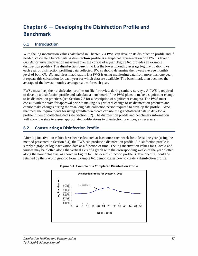
Disinfection Profiling and Benchmarking 47 Technical Guidance Manual
Chapter 6 — Developing the Disinfection Profile and Benchmark
6.1 Introduction
With the log inactivation values calculated in Chapter 5, a PWS can develop its disinfection profile and if needed, calculate a benchmark. A disinfection profile is a graphical representation of a PWS’s level of Giardia or virus inactivation measured over the course of a year (Figure 6-1 provides an example disinfection profile). The disinfection benchmark is the lowest monthly average log inactivation. For each year of disinfection profiling data collected, PWSs should determine the lowest average monthly level of both Giardia and virus inactivation. If a PWS is using monitoring data from more than one year, it repeats this calculation for each year for which data are available. The benchmark then becomes the average of the lowest monthly average values for each year.
PWSs must keep their disinfection profiles on file for review during sanitary surveys. A PWS is required to develop a disinfection profile and calculate a benchmark if the PWS plans to make a significant change to its disinfection practices (see Section 7.2 for a description of significant changes). The PWS must consult with the state for approval prior to making a significant change to its disinfection practices and cannot make changes during the year-long data collection period required to develop the profile. PWSs that meet the requirements for using grandfathered data can use the grandfathered data to develop a profile in lieu of collecting data (see Section 3.2). The disinfection profile and benchmark information will allow the state to assess appropriate modifications to disinfection practices, as necessary.
6.2 Constructing a Disinfection Profile
After log inactivation values have been calculated at least once each week for at least one year (using the method presented in Section 5.4), the PWS can produce a disinfection profile. A disinfection profile is simply a graph of log inactivation data as a function of time. The log inactivation values for Giardia and viruses may be plotted along the vertical axis of a graph with the corresponding weeks of the year plotted along the horizontal axis, as shown in Figure 6-1. After a disinfection profile is developed, it should be retained by the PWS in graphic form. Example 6-1 demonstrates how to create a disinfection profile.
Figure 6-1. Example of a Completed Disinfection Profile
0.0000.2000.4000.6000.8001.0001.2001.400
0 4 8 12 16 20 24 28 32 36 40 44 48 52
Log
Inac
tivat
ion
Week Tested
Disinfection Profile for System X, 2016
Log Inactivation

Disinfection Profiling and Benchmarking 48 Technical Guidance Manual
Example 6-1. Disinfection Profile for Giardia
Create a disinfection profile for Giardia for the conventional filtration system that was discussed in Examples 3-1, 4-1, 4-2, 5-1, and 5-2.
Step 1. Calculate the Giardia log inactivation once per week on the same day of the week for one year.
The table below shows the Giardia logs of inactivation that were calculated each week for one year using the methods presented in Section 5.4 and Example 5-2. This information can also be obtained from the first and last columns of Worksheet #1 in Appendix C for PWSs with one disinfection segment or Worksheet #2 in Appendix C for PWSs with multiple disinfection segments.
Month Week Log Inactivation Month Week Log Inactivation
JAN 1 1.34 JULY 27 1.86
2 1.35 28 1.82
3 1.38 29 1.76
4 1.37 30 1.74
5 1.38 31 1.71
FEB 6 1.38 AUG 32 1.70
7 1.39 33 1.66
8 1.40 34 1.61
9 1.40 35 1.60
MARCH 10 1.40 SEP 36 1.55
11 1.41 37 1.56
12 1.42 38 1.52
13 1.43 39 1.51
APRIL 14 1.46 40 1.47
15 1.50 OCT 41 1.48
16 1.54 42 1.47
17 1.57 43 1.47
18 1.64 44 1.45
MAY 19 1.66 NOV 45 1.41
20 1.70 46 1.43
21 1.72 47 1.41
22 1.74 48 1.40
JUNE 23 1.77 DEC 49 1.40
24 1.79 50 1.40
25 1.82 51 1.40
26 1.81 52 1.37

Disinfection Profiling and Benchmarking 49 Technical Guidance Manual
Step 2. Plot the disinfection profile.
The logs of inactivation are plotted along the vertical axis with the corresponding weeks of the year plotted along the horizontal axis. For example, the log inactivation value for week 1 (1.34) is plotted on the vertical axis at a point corresponding to week 1 on the horizontal axis, as shown below. The log inactivation value for week 2 (1.35) is plotted on the horizontal axis at a point corresponding to week 2 on the horizontal axis. The log inactivation value for week 3 (1.38) is plotted on the horizontal axis at a point corresponding to week 3 on the horizontal axis. After the points are plotted, lines are drawn to connect the points in order by the week tested.
Week Tested(Horizontal Axis)
1 2
1.35
1.40
Log
Inac
tivat
ion
(Ver
tical
Axi
s)
1.303
Continue to plot the points for each week until all 52 weeks have been plotted. The completed disinfection profile is shown below.
0.0
0.5
1.0
1.5
2.0
1/1/2016 3/25/2016 6/17/2016 9/9/2016 12/2/2016
Gia
rdia
Log
Inac
tivat
ion
Sample Date
Once a disinfection profile has been completed, the PWS will have all of the data required to calculate a benchmark. The following sections discuss what a benchmark is and how it is calculated.

Disinfection Profiling and Benchmarking 50 Technical Guidance Manual
6.3 Calculating the Disinfection Benchmark
As explained in Chapter 1, benchmarking is used to characterize the minimum level of Giardia and virus logs of inactivation that were achieved under existing disinfection practices. A benchmark calculated under existing conditions can be compared to the benchmark calculated for anticipated conditions once proposed modifications are made. This comparison helps to ensure that changes to disinfection practices that result in lower inactivation levels are not made without appropriate state consultation and review. A disinfection benchmark is calculated using the following steps:
• Complete a disinfection profile that includes the calculation of log inactivation of Giardia and viruses for each week of the profile.
• Compute the average log inactivation for each calendar month of the profile by averaging the log inactivation values for each month (see Equation 6-1).
Equation 6-1
Monthly Average Log Inactivation =
Sum of Log Inactivation Values for the Month
Number of Values per Month
Select the month with the lowest average log inactivation for the 12-month period. This value is the benchmark.
Example 6-2 demonstrates how to calculate the disinfection benchmark.
Example 6-2. Calculating a Disinfection Benchmark
Calculate the disinfection benchmark for Giardia for the conventional filtration system discussed in Examples 3-1, 4-1, 4-2, 5-1, 5-2, and 6-1.
Step 1. Calculate weekly Giardia log inactivation.
This step was completed in Example 6-1. The data are summarized below:
Month Week Log Inactivation Month Week Log Inactivation
JAN 1 1.34 JULY 27 1.86
2 1.35 28 1.82
3 1.38 29 1.76
4 1.37 30 1.74
5 1.38 31 1.71
FEB 6 1.38 AUG 32 1.70
7 1.39 33 1.66
8 1.40 34 1.61

Disinfection Profiling and Benchmarking 51 Technical Guidance Manual
Month Week Log Inactivation Month Week Log Inactivation
9 1.40 35 1.60
MARCH 10 1.40 SEP 36 1.55
11 1.41 37 1.56
12 1.42 38 1.52
13 1.43 39 1.51
APRIL 14 1.46 40 1.47
15 1.50 OCT 41 1.48
16 1.54 42 1.47
17 1.57 43 1.47
18 1.64 44 1.45
MAY 19 1.66 NOV 45 1.41
20 1.70 46 1.43
21 1.72 47 1.41
22 1.74 48 1.40
JUNE 23 1.77 DEC 49 1.40
24 1.79 50 1.40
25 1.82 51 1.40
26 1.81 52 1.37
Step 2. Calculate the monthly average log inactivation for each month.
Begin by averaging January’s inactivation values:
Average log Sum of Log Inactivation Values
inactivation for January = Number of Values in Month
Average log 1.34 + 1.35 + 1.38 + 1.37 + 1.38
inactivation for January = 5 values
= (6.82) / (5) = 1.36
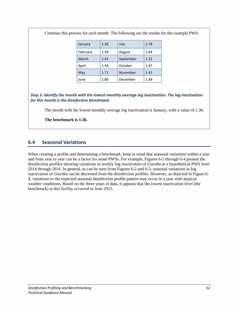
Disinfection Profiling and Benchmarking 52 Technical Guidance Manual
Continue this process for each month. The following are the results for the example PWS:
January 1.36 July 1.78
February 1.39 August 1.64
March 1.41 September 1.52
April 1.54 October 1.47
May 1.71 November 1.41
June 1.80 December 1.39
Step 3. Identify the month with the lowest monthly average log inactivation. The log inactivation for this month is the disinfection benchmark.
The month with the lowest monthly average log inactivation is January, with a value of 1.36.
The benchmark is 1.36.
6.4 Seasonal Variations
When creating a profile and determining a benchmark, keep in mind that seasonal variations within a year and from year to year can be a factor for some PWSs. For example, Figures 6-2 through 6-4 present the disinfection profiles showing variations in weekly log inactivation of Giardia at a hypothetical PWS from 2014 through 2016. In general, as can be seen from Figures 6-2 and 6-3, seasonal variations in log inactivation of Giardia can be discerned from the disinfection profiles. However, as depicted in Figure 6-4, variations to the expected seasonal disinfection profile pattern may occur in a year with atypical weather conditions. Based on the three years of data, it appears that the lowest inactivation level (the benchmark) at this facility occurred in June 2015.

Disinfection Profiling and Benchmarking 53 Technical Guidance Manual
Figure 6-2. 2014 Data
0.0
2.0
4.0
6.0
8.0
10.0
12.0
14.0
16.0
Log
Gia
rdia
Inac
tivat
ion
Figure 6-3. 2015 Data
0.0
2.0
4.0
6.0
8.0
10.0
12.0
14.0
16.0
Log
Gia
rdia
Inac
tivat
ion
Figure 6-4. 2016 Data
0.0
2.0
4.0
6.0
8.0
10.0
12.0
14.0
16.0
Log
Gia
rdia
Inac
tivat
ion

6.5 The Complete Profile and Benchmark
PWSs should keep the completed disinfection profile and supporting data on file at the treatment plant or the PWS’s offices in graphical form, as a spreadsheet, or in some other format approved by the state. In the event the PWS decides to modify its disinfection practice, the disinfection profile must be used to create a benchmark.
6.6 Steps Completed
Identify Disinfection Segments
Collect Data
Calculate CT
Calculate Inactivation
Develop the Disinfection Profile and Benchmark
Evaluate the Disinfection Profile and Benchmark
6.7 Next Step
Upon completing the activities in this chapter, the PWS will have completed the fifth of six steps: developing a disinfection profile and benchmark. By calculating the benchmark, the PWS has identified its lowest monthly average inactivation value. This benchmark is used as a guide when evaluating disinfection practice modifications. Chapter 7 provides information on how to evaluate disinfection practice modifications.
Disinfection Profiling and Benchmarking 54 Technical Guidance Manual

Disinfection Profiling and Benchmarking 55 Technical Guidance Manual
Chapter 7 — Evaluating Disinfection Practice Modifications
7.1 Introduction
Compliance with the Stage 2 DBPR LRAA MCLs or requirements to provide additional treatment for Cryptosporidium may result in a PWS making significant modifications to their current disinfection practices. If a benchmark value is less than the required log inactivation, then the PWS can consider increasing the amount of disinfectant or the contact time. But increasing the amount of disinfectant could increase DBPs. If the benchmark is greater than the required inactivation in Table 1-2 (or as required by the state), the PWS can consider decreasing the amount of disinfectant added or altering other disinfection practices to continue to meet the required CT to decrease the formation of DBPs. Changes to disinfection practices that are considered significant are discussed in detail in this chapter. The purpose of disinfection profiling and benchmarking, and its usefulness to the state and the PWS are also discussed here.
The following terms may be helpful for understanding disinfection practices:
• DBP Precursors – DBP precursors are constituents naturally occurring in source water that react with a disinfectant to form DBPs. The primary DBP precursor is natural organic matter, which is monitored as total organic carbon (TOC). Organic matter reacts with the disinfectant to form TTHM, HAA5, and other DBPs. The Alternative Disinfectants and Oxidants Guidance Manual (USEPA, April 1999) provides more detailed information on DBP formation.
• Pre-disinfection – Pre-disinfection occurs when a disinfectant is added to the treatment train prior to the primary disinfectant injection location. The purpose of pre-disinfection is to obtain additional inactivation credits, to control microbiological growth in subsequent treatment processes, to improve coagulation, and/or to reduce tastes and odors.
• Primary Disinfection – The disinfectant used in a treatment system with the primary objective to achieve the necessary microbial inactivation.
• Secondary Disinfection – The disinfectant applied following primary disinfection in a treatment system with the primary objective to maintain the residual disinfectant throughout the distribution system.
7.2 Significant Changes to Disinfection Practices
As listed in Section 1.3, the IESWTR, LT1ESWTR, and LT2ESWTR describe four types of significant changes to disinfection practices. Those significant changes and related considerations are discussed in greater detail below.
7.2.1 Changes to the Point of Disinfection
Any change in the location of the disinfectant application constitutes a significant change to disinfection practices. For instance, a PWS that uses pre-disinfection may consider moving the point of disinfectant application further downstream in the treatment train (see Figure 7-1). This modification can result in:
• A reduction of contact time (T) between DBP precursors and the disinfectant(s).

Disinfection Profiling and Benchmarking 56 Technical Guidance Manual
• A reduction in the production of DBPs (particularly if the new location is at a location downstream of treatment processes that have removed organic compounds that are precursors to DBP formation).
• A reduction of contact time (T) for inactivation.
A PWS that is considering moving the point of disinfectant application further downstream in the treatment process should ensure that it can maintain adequate disinfectant contact time and meet required log inactivation requirements for Giardia and viruses under the modified disinfecting conditions. Figure 7-1 shows an example of a PWS that considers relocating its pre-disinfection location.
Figure 7-1. Example of Moving the Point of Pre-disinfectant Application
DistributionSystem
Sedimentation
Coagulation
ClearwellIntake
PredisinfectionLocation
1 1 1
Cl2Feed
Filtration
Flocculation
1 Potential locations for pre-disinfection. For example, the PWS may consider relocating the pre-disinfection location from the intake to one of three other possible locations. The potential for DBP formation decreases further downstream in the treatment train for two reasons:
1. Contact time between DBP precursors and disinfectants is reduced. 2. DBP precursors are removed with each subsequent treatment process.
7.2.2 Changes to Disinfectant Type
If a PWS is considering changing or adding a disinfectant, it is important to understand that each disinfectant has different levels of inactivation effectiveness for different types of pathogens. As a result, the CT requirements for the various disinfectants can be radically different. For instance, the CT required for chloramines to achieve 1-log inactivation of Giardia is about 18 times greater than the CT required for free chlorine. Therefore, if a PWS is considering changing from chlorine to chloramines, CT will have to be achieved either by raising the residual concentration in the disinfection zone or by increasing the contact time. A brief discussion of alternative disinfectants and oxidants that a PWS may consider is provided in Chapter 8.
Figure 7-2 is an example of a PWS that considers changing its disinfectant type. Figure 7-3 discusses a case where a change in both point of disinfection and disinfectant type are being considered.

Disinfection Profiling and Benchmarking 57 Technical Guidance Manual
Figure 7-2. Example of Changing Disinfectant Type
DistributionSystem
Clearwell
Primary Disinfectant(Existing)
Cl2Feed
Secondary Disinfectant (New)Ammonia Feed for
Monochloramine Formation
From Filtration
Under existing conditions, chlorine is used as the sole disinfectant and is added prior to the clearwell to obtain Giardia and virus inactivation. The PWS has decided to add ammonia after the clearwell to produce chloramine. Using chloramines as a secondary disinfectant has two advantages:
1. Chloramines should result in lower TTHM and HAA5 formation in the distribution system, as they typically have a lower potential for TTHM and HAA5 formation than chlorine.
2. Chloramine residuals usually last longer than chlorine residuals in the distribution system.
Figure 7-3. Changing Pre-disinfection Location and Type of Disinfectant
DistributionSystem
SedimentationPre-Sedimentation
Coagulation
ClearwellIntake
ClFeed
Chlorine(point 1)
Ozone(point 2)
Filtration
Under existing conditions, the PWS was using chlorine as a pre-disinfectant prior to pre-sedimentation and final disinfection prior to the clearwell. The PWS has decided to change the pre-disinfection location from prior to the pre-sedimentation basin (point 1) to prior to coagulation (point 2), in order to decrease contact time and reduce DBP formation due to the organic-rich supply water prior to pre-sedimentation. In addition, they are considering changing pre-disinfection from chlorine to ozone which may help reduce TTHM and HAA5 formation, but consequently, could result in the formation of bromate if sufficient levels of bromide are present in the water.

Disinfection Profiling and Benchmarking 58 Technical Guidance Manual
7.2.3 Changes to the Disinfection Process
Changes to the disinfection process itself also require PWSs to consult with the state before making the treatment change. Some modifications to the disinfection process include the following:
• Changing the contact basin geometry and baffling conditions. • Changing the pH during disinfection. • Decreasing the disinfectant dose during warmer temperatures. • Increasing or decreasing flow through the plant.
Effects of Basin Geometry and Baffling Conditions
Changing the contact basin geometry or baffling conditions may result in more inactivation by increasing the contact time, the T value in the CTcalc value. The basin geometry changes the TDT while the baffling conditions change the BF in Equation 4-3 used to determine T (see Section 4.4.4). With this type of modification, additional inactivation can be achieved without increasing the disinfectant concentration.
pH Effects on Chlorine
Chlorine is very sensitive to pH. Decreases in pH provide increased chlorine inactivation of Giardia and viruses. Therefore, at lower pH values a lower chlorine dose or contact time can be applied to achieve a comparable level of inactivation of both Giardia and viruses. This in turn can reduce the potential for DBP formation. However, decreasing the pH is a process-sensitive issue and could result in other system changes, such as increased coagulant demand for proper floc formation, distribution system corrosion problems which, depending on a customer’s plumbing or service connection type, could result in violations of the Lead and Copper Rule, or precipitation of certain inorganics. Extensive jar tests and pilot scale studies may be necessary before adjusting the pH.
Temperature Effects on Chlorine and DBP Formation
Chlorine is more effective at higher water temperatures, which results in faster chemical reactions and consequently, greater potential for DBP formation. Warmer surface waters frequently support more organic growth, supplying higher levels of DBP precursors. However, since chlorine is more reactive at higher temperatures, it is also more effective against microorganisms such as Giardia and viruses. Thus, when water temperatures are warmer the chlorine dose or contact time can be decreased and achieve the same amount of microbial inactivation as in cooler temperatures. However, warm temperatures also result in quicker chlorine decay so maintaining chlorine residual and microbial control in the distribution system could be adversely affected if the chlorine dose is decreased in the treatment plant. If a PWS decreases the chlorine dose or contact time during warmer months, the PWS should ensure that it is maintaining sufficient inactivation of both Giardia and viruses and also maintaining chlorine residual and microbial control in the distribution system.
7.2.4 Other Modifications
The modifications listed in Sections 7.2.1 through 7.2.3 are not an exhaustive list. States may determine that other types of changes are also significant. Therefore, a PWS should check with the state program office for assistance with determining whether a proposed change triggers the disinfection benchmarking procedure. Other modifications that may require state consultation and approval are enhanced coagulation, enhanced softening or oxidation. In addition, increased flow through the plant will have a direct impact on contact time. PWSs should work with the state to determine at what point increases in

Disinfection Profiling and Benchmarking 59 Technical Guidance Manual
plant flow constitute a change to disinfection practices. PWSs can refer to the Alternative Disinfectants and Oxidants Guidance Manual (USEPA, April 1999) and the Enhanced Coagulation and Enhanced Precipitative Softening Guidance Manual (USEPA, May 1999) for additional information. Copies of these guidance manuals can be obtained by downloading from the EPA’s website at https://www.epa.gov/dwreginfo/guidance-manuals-surface-water-treatment-rules.
7.3 How the State Will Use the Benchmark
The state is expected to use the disinfection profile and benchmark to evaluate the microbial inactivation a PWS has achieved over time and compare this with the expected microbial inactivation the PWS will achieve after proposed disinfection practice modifications are made. The benchmark may be used by the state as a minimum level of inactivation of Giardia and viruses that must be maintained by PWSs when modifying their disinfection practices. The state may also use the disinfection profile and benchmark to determine an appropriate alternative benchmark under different disinfection scenarios.
PWSs with a benchmark that is less than the inactivation requirements in Table 1-2 or state-approved inactivation requirements (if they differ from Table 1-2) will need to modify disinfection practices in order to provide the necessary level of disinfection. An example would be a PWS with a conventional treatment plant that has calculated a benchmark of 0.3 for Giardia but is required to achieve 0.5-log Giardia inactivation through disinfection. This PWS would need to provide additional disinfection to achieve the required 0.5-log Giardia inactivation. At the same time, the PWS must ensure it maintains compliance with the DBPRs. The PWS must consult with the state and provide all necessary information prior to any significant modification, as described in Section 7.2.
PWSs may consider modifying disinfection practices if the benchmark is greater than the inactivation requirements in Table 1-2 or the inactivation required by the state. An example would be a PWS with a conventional treatment plant that has calculated a benchmark of 1.3 for Giardia but is only required to achieve a 0.5-log Giardia inactivation through disinfection. If this PWS uses chlorine and is having difficulty complying with TTHM and HAA5 MCLs, it may consider decreasing the number of chlorine injection points it utilizes. However, it must determine the CT needed to meet the 0.5-log Giardia inactivation as it tries to maintain compliance with the DBPRs. Again, the PWS must consult with the state prior to making any significant modifications and must provide all necessary information.

Disinfection Profiling and Benchmarking 60 Technical Guidance Manual
7.4 Steps Completed
Upon completing the activities in this chapter, the PWS will have completed all six steps in disinfection profiling and benchmarking.
Identify Disinfection Segments
Collect Data
Calculate CT
Calculate Inactivation
Develop the Disinfection Profile and Benchmark
Evaluate the Disinfection Profile and Benchmark
7.5 References
USEPA. April 1999. Alternative Disinfectants and Oxidants Guidance Manual. EPA 815-R-99-014. Washington, D.C.
USEPA. May 1999. Enhanced Coagulation and Enhanced Precipitative Softening Guidance Manual. EPA 815-R-99-012. Washington, D.C.

Disinfection Profiling and Benchmarking 61 Technical Guidance Manual
Chapter 8 — Treatment Considerations
8.1 Introduction
As PWSs comply with the Stage 2 DBPR LRAA MCLs or requirements to provide additional treatment for Cryptosporidium, they may need to make significant modifications to their existing disinfection practices. This chapter summarizes different treatment options available to PWSs when considering such modifications. Some methods that PWSs may use to control DBPs, while meeting the inactivation levels required for Giardia and viruses, include the use of alternative disinfectants and oxidants, enhanced coagulation and softening, decreasing the contact time, or the use of alternative filtration techniques, such as membranes. PWSs may also opt to use chlorine dioxide, ozone, UV, or membrane filtration for Cryptosporidium treatment under the LT2ESWTR. As discussed in Chapter 7, the state must be consulted prior to any significant modifications to existing systems.
8.2 Alternative Disinfectants and Oxidants
This section discusses various alternative disinfectants and oxidants that may be considered for meeting both microbial inactivation and disinfection byproduct standards. A more complete discussion of this topic is provided in the Alternative Disinfectants and Oxidants Guidance Manual (USEPA, April 1999).
Retaining an adequate disinfectant residual at all points in the distribution system is important to inhibit bacteriological growth and using chlorine to achieve this has been a widely accepted practice, particularly in small PWSs. Chlorine is typically used in one of three forms: chlorine gas, sodium hypochlorite (typically liquid), and calcium hypochlorite (typically solid). Chlorine effectively inactivates a wide range of pathogens, including Giardia and viruses. Chlorine residuals are generally carried into the distribution system for further protection (see Example D1 in Appendix D).
However, the use of chlorine as a disinfectant, particularly as a pre-disinfectant, has typically been found to increase the formation of DBPs. The long detention time for water at the extremities of the distribution system also promotes DBP formation when chlorine is used. One option for resolving this problem is to use alternate primary disinfectants such as chlorine dioxide, ozone, or UV light. Other options are to add potassium permanganate as a pre-oxidant instead of chlorine or to use chloramines to maintain the distribution system residual. The type of oxidant used, its point of application and its concentration have significant effects on DBP formation. Consideration should also be given to the pH of the water, since lowering the pH decreases TTHM formation but increases formation of other chlorinated organic chemicals or forms of halomethanes (Dowbiggin and Thompson, 1990). In addition, higher water temperatures speed up the reaction between chlorine and organic material, thus increasing finished water TTHM and HAA5 levels (Singer, 1999).
8.2.1 Chloramines (NH2Cl)
Chloramines are formed when chlorine and ammonia are added to the water, either simultaneously or sequentially. Chloramination is normally practiced at a ratio of approximately 1 part of ammonia to 4 parts of chlorine (on a mg/L basis) to ensure monochloramine formation (Kawamura, 2000). The ammonia can be applied before or after the chlorine. However, applying ammonia after the chlorine has been found to inactivate pathogens more effectively (AWWA, 1999). The CT tables presented in Appendix B of this guidance assume ammonia is added after chlorine to form chloramines. The CT tables illustrate that chloramines require significantly more contact time than chlorine to meet the required inactivation of Giardia and viruses.

Disinfection Profiling and Benchmarking 62 Technical Guidance Manual
Using chloramine as a secondary disinfectant has two advantages: 1) chloramine typically has a lower potential for TTHM and HAA5 formation than chlorine; and 2) chloramine residuals last longer than chlorine. Monochloramine is effective for controlling bacterial regrowth due to its ability to penetrate pipe biofilm (USEPA, April 1999). When chloramines are formed for secondary disinfection, ammonia is added to the treated water after the water treatment plant clearwell where primary disinfection is accomplished.
Potential water quality issues with monochloramine include corrosion, formation of DBPs, and nitrification. Monochloramine can impact kidney dialysis and should be removed from the dialysate water. Monochloramine should be removed from water used, for example, fish tanks due to detrimental effects. The use of monochloramine can cause pitting corrosion and a more uniform thinning of pipe surfaces (Kirmeyer et al., 2004). Kirmeyer et al. (2004) also reported that chloramine can attack rubber and plastic components in a water system, and that 43 percent of utilities surveyed experienced an increase in degradation of rubber materials. Although chloramination significantly reduces some DBPs associated with chlorine disinfection, such as THM and HAAs, its usage can contribute to the formation of other DBPs such as nitrosamines. Nitrification is a potential problem for utilities that utilize chloramines as a disinfectant and may occur when finished water contains excess ammonia and low chloramine residual (Kirmeyer et al., 2004). Areas of the distribution system with higher water age and warmer temperatures are more susceptible to nitrification.
8.2.2 Ozone (O3)
One of the most widely studied alternatives to chlorine as a disinfectant is ozone. Ozone is used for both oxidation and disinfection. It must be generated at the point of application since it is an unstable molecule. Ozone is a powerful oxidant and is more effective than chlorine, chloramines, and chlorine dioxide for inactivation of viruses, Cryptosporidium, and Giardia (USEPA, April 1999). Its effectiveness is pH and temperature dependent. Ozone can only be used as a primary disinfectant, since it is unable to maintain a residual in the distribution system. Chlorine or chloramines should be applied as a secondary disinfectant to maintain a detectable residual in the distribution system. The following case study (Schneider and Tobiason, 2000) discusses bench-scale studies using ozone as a pre-disinfectant prior to coagulation and its impact on the coagulation process using various coagulants.
Ozone is highly corrosive and toxic, and ozonation systems are relatively complex. The use of ozone poses some health and safety concerns that should be addressed by a utility considering its use. Instrumentation should be provided for ozone systems to protect both personnel and the equipment. While ozone does not form halogenated DBPs except in bromide-rich waters, it does form a variety of organic and inorganic byproducts, such as bromate. Bromate is regulated by the Stage 1 DBPR with an MCL of 0.010 mg/L.
8.2.3 Chlorine Dioxide (ClO2)
Chlorine dioxide is a powerful oxidant and disinfectant that is effective at inactivating bacterial, viral, and protozoan pathogens (e.g., Giardia and Cryptosporidium). Chlorine dioxide is equal or superior to chlorine in its disinfecting ability. Chlorine dioxide is primarily used in the United States as a means of taste and odor control, oxidation of iron and manganese, and control of TTHMs and HAA5s by oxidizing precursors (Kawamura, 2000). It also has the ability to maintain a residual in the distribution system for an extended period of time (Kawamura, 2000).

Disinfection Profiling and Benchmarking 63 Technical Guidance Manual
Chlorine dioxide is usually generated on site from sodium chlorite solutions and one or more other chemical precursors (e.g., sodium hypochlorite, hydrochloric acid, sulfuric acid) or by an electrochemical oxidation process. Stock solutions produced on-site typically have a concentration of 500 mg/L. Chlorine dioxide gas cannot be compressed or stored commercially because it is explosive under pressure. Therefore, chlorine dioxide gas is never shipped (USEPA, December 1999).
Chlorine dioxide and chlorite, a disinfection byproduct of concern for PWSs using chlorine dioxide, are both regulated by the Stage 1 DBPR. The Stage 1 DBPR establishes an MRDL of 0.8 mg/L as ClO2 that applies to all PWSs (CWS, NTNCWS, and transient non-community water systems (TNCWS)) using chlorine dioxide because chlorine dioxide can present an acute health risk at high enough levels. All PWSs that use chlorine dioxide must monitor for compliance with the MRDL daily at the entry point to the distribution system. The Stage 1 DBPR also establishes a chlorite MCL of 1.0 mg/L for systems that use chlorine dioxide for disinfection and oxidation. CWSs and NTNCWSs must collect daily samples at the entry point to the distribution system and monthly samples in the distribution system. Utilities using chlorine dioxide may have to use granular activated carbon or a chemical reducing agent, such as sulfur dioxide, to remove or reduce the chlorite residual.
8.2.4 Potassium Permanganate (KMnO4)
Potassium permanganate is primarily used as a pre-oxidant to control algal growth; tastes and odors; and to remove iron, manganese, and color. It may also be used to control DBP formation by oxidizing organic precursors and reducing the demand for other disinfectants (USEPA, April 1999). A water treatment plant may choose to use potassium permanganate as a pre-oxidant, in lieu of chlorine, and then move the chlorination point further down the treatment train. This configuration may help control DBPs by delaying the introduction of chlorine until after the majority of precursors have been removed in the treatment process.
There are some disadvantages to using potassium permanganate. Potassium permanganate must be handled carefully when preparing the feed solution, since it can cause serious eye injury, irritate the skin and respiratory system, and can be fatal if swallowed. It also can turn the water a pink color.
Case Study – Schneider and Tobiason (2000)
Jar-testing was used to study the effects of pre-ozonation on interactions among coagulants, particles, and natural
organic matter. Synthetic water (deionized, distilled water with organic matter, particles and background ions added) and waters from Lake Gaillard in Branford,
Connecticut; the Oradell reservoir in Oradell, New Jersey; and the Passaic River in Little Falls, New Jersey, were
tested. Experiments were run with ozone only and with ozone followed by coagulation. The research found that
when alum was used as a coagulant, pre-ozonation hindered the removal of turbidity and dissolved organic
matter (DOM) at the conditions tested. Cationic polymers, however, allowed small increases in the removal of
turbidity and DOM. It was found that varying the pre-ozone contact time from 4 to 28 minutes had little effect
on settled water turbidity, TOC, and dissolved organic carbon for the conditions tested.

Disinfection Profiling and Benchmarking 64 Technical Guidance Manual
8.2.5 Ultraviolet Radiation (UV)
UV disinfection is a well-established treatment technology for inactivating pathogens present in the environment. In the drinking water context, UV disinfection was initially most widely used in Europe, with hundreds of installations in place by 1985 (USEPA, November 2006). In North America, UV disinfection has been more widely employed in drinking water applications since 2000 to address health concerns associated with Cryptosporidium. As of the spring of 2008, there were at least 300 public water systems in the United States and Canada with UV installations treating flows >350 gallons per minute (Wright et al., 2012).
UV disinfection does not cause the formation of harmful disinfection byproducts and is highly effective for inactivating Cryptosporidium and Giardia. UV rays inactivate microorganisms by penetrating their cell walls to damage the DNA, interfering with reproduction. An additional advantage is that there are fewer safety concerns for using UV than for chemical disinfectants such as chlorine gas or chlorine dioxide. Further, UV disinfection does not change the pH or the corrosivity of the treated water (USEPA, April 2006).
The EPA’s Ultraviolet Disinfection Guidance Manual for the Final Long Term 2 Enhanced Surface Water Treatment Rule (UVDGM) (USEPA, November 2006) provides guidance to PWSs using UV light for primary disinfection. The UV dose is expressed in millijoules per square centimeter (mJ/cm2) or the equivalent, milliwatt-seconds per square centimeter (mW·s/cm2). The dose required to achieve a 2-log inactivation of Cryptosporidium and Giardia are 5.8 mJ/cm2 and 5.2 mJ/cm2, respectively. However, the dose required for virus inactivation is quite a bit higher, at 100 mJ/cm2 for 2-log inactivation and 186 mJ/cm2 for 4-log inactivation. Many PWSs use a combination of UV light for its ability to inactivate Cryptosporidium and Giardia, as well as chlorine that is highly effective for virus inactivation and then also carries a residual into the distribution system.
UV reactor validation is used to define the operational conditions under which the pathogens of concern are inactivated for a specific UV reactor manufacturer and model. Validation is a method of determining the operating conditions under which a UV reactor delivers a specified dose. This generally involves initial tests using a surrogate organism (e.g., bacteriophage MS2) rather than the target pathogen (e.g., Cryptosporidium) to establish the dose relationship between the two organisms. The conditions that are examined for full-scale testing to establish dose are flow rate, UV transmittance (UVT) (a measure of the fraction of incident light transmitted through a material) and lamp output. The EPA has developed guidance for validation of UV reactors (USEPA, November 2006) using one of two methods – the setpoint approach and the dose control method. In short, the setpoint approach establishes a measured UV intensity that corresponds to a specific dose and flow rate. The dose control method (also referred to as the calculated dose approach) provides a means of determining the required intensity that corresponds to a specific flow rate, UVT, and dose.
Despite the many advantages of UV light for primary disinfection, these systems also have some shortcomings.
• UV disinfection is less effective at inactivating some viruses, particularly adenovirus.
• Since UV is a physical disinfectant, not a chemical disinfectant, it does not leave a residual in the water and thus, a secondary disinfectant must be added to maintain a distribution system residual.
• Another disadvantage is that higher turbidity and organic material in the water may shield organisms and prevent them from being exposed to the UV light; therefore, it is recommended

Disinfection Profiling and Benchmarking 65 Technical Guidance Manual
that PWSs apply UV light as a disinfectant after filtration, where turbidity and organics in the water have been reduced.
• Another potential problem is that scale can form on the quartz sleeves that house the UV lamps, depending on the ions, hardness, alkalinity, and pH of the water. For example, a hardness level greater than 120 mg/L is a threshold of concern (Great Lakes, 2018). A build-up of scale causes a reduction in the amount of UV light that is transmitted to the water. However, regular cleaning of the sleeves can reduce the effects of scaling.
• Mercury can be released into the treated water when a UV lamp breaks (Wright et al., 2012). The amount of mercury that could potentially enter the water depends on the type of lamp and operation. Vapor phase mercury can dissolve into solution and be discharged downstream whereas liquid phase or amalgam mercury would tend to settle in the UV reactor. The author recommends developing a mercury mitigation plan (Wright et al., 2012).
• The use of UV light in a water treatment plant introduces several potential safety issues for operators including exposure of skin and eyes to UV light; electrical shock; burns from hot lamps or equipment; and exposure to mercury from a broken lamp. Safety measures must be developed and implemented to address each potential safety issue.
• Finally, the operation of the UV lamps may be temperature dependent. UV lamps are designed to operate within a specific temperature range to maximize UV light output (USEPA, November 2006). Without flowing water to cool the lamp, the lamp temperature can rise above the maximum operating temperature and break.
8.2.6 Comparison of Disinfectants
The EPA and the Association of Metropolitan Water Agencies (AMWA) funded a two-year study of 35 water treatment facilities to evaluate DBP production based on various combinations of primary and secondary disinfectants. Among four of the facilities, alternative disinfection strategies were investigated to evaluate the difference in DBP production from the PWSs’ previous disinfection strategies (or base disinfection conditions). The results were analyzed in three reports (Metropolitan and Montgomery, 1989; Jacangelo et al., 1989; Malcolm Pirnie, Inc., 1992) that documented different aspects of the study. Table 8-1 summarizes the results of the study. This study illustrates that a change in primary disinfectant from chlorine to ozone or to chloramines may help reduce TTHM and HAA5.
Table 8-1. Study Results on Changing Primary and Secondary Disinfectants
Change in Disinfection Practice1 (Primary Disinfectant/Secondary Disinfectant)
DBP Concentration Change
TTHM HAA5
Chlorine/Chlorine To
Chlorine/Chloramines2
Utility #7 Decrease Decrease
Chlorine/Chlorine To
Ozone/Chlorine
Utility #19 Decrease Decrease
Utility #36 No change No change
Chlorine/Chloramines To
Utility #7 Decrease Decrease

Disinfection Profiling and Benchmarking 66 Technical Guidance Manual
Ozone/Chloramines
Chlorine/Chlorine To
Chloramines/Chloramines
Utility #36 Decrease Decrease
Ozone/Chlorine To
Ozone/Chloramines
Utility #36 Decrease Decrease
Chloramines/Chloramines To
Ozone/Chloramines
Utility #25 Decrease Decrease
Utility #36 No change No change
Chlorine/Chlorine To
Ozone/Chloramines
Utility #7 Decrease Decrease
Utility #36 Decrease Decrease
1. Several studies were conducted to examine the effects of changing primary and secondary disinfectants on DBP levels. For instance, changing the secondary disinfectant from chlorine to chloramines resulted in a decrease in both TTHM and HAA5. Results are based on full-scale evaluations at Utilities #19 and #25 and on pilot scale evaluations at Utilities #7 and #36. 2. Free chlorine contact time was 4 hours for Utility #7 during use of chlorine/chloramine strategy. Source: Malcolm Pirnie, Inc., 1992; Jacangelo et al., 1989.
8.3 Changes in Enhanced Coagulation and Softening
In conventional water treatment plants, precursors of DBPs may be removed through the coagulation process with aluminum or ferric salts and/or polymers. If a greater reduction in DBP levels is required, the treatment techniques of either enhanced coagulation or enhanced precipitative softening can be employed. With fewer precursors present, the formation of DBPs is thereby reduced. Enhanced coagulation also allows for more effective disinfection, since the chlorine demand is lower in water treated by enhanced coagulation. In addition, the lower pH resulting from enhanced coagulation allows chlorine to inactivate Giardia more effectively, since chlorine is more effective at lower pH values.
One way to implement enhanced coagulation is to change the type or dose of coagulant and/or polymer aid. However, before either enhanced coagulation or enhanced softening is implemented at a water treatment plant, the proposed changes should be evaluated through pilot testing or bench-scale studies similar to the case study by Bell-Ajy et al. (2000) described in the text box below. Jar testing is commonly used to simulate coagulant dose changes and their effectiveness. A water treatment plant operator should first determine the present status of the coagulation process by taking TOC samples from the raw water and the finished water. With these data, the operator can calculate the percent removal of TOC and determine a desired TOC removal.

Disinfection Profiling and Benchmarking 67 Technical Guidance Manual
Case Study - Bell-Ajy et al. (2000)
Research, including jar tests using raw water from 16 water utilities throughout the United States and two full-scale evaluations, was conducted to evaluate the optimal coagulation conditions for removal of TOC and DBPs. Jar test results showed that when optimized coagulation was implemented, treatment effectiveness seemed pH dependent. Jar tests using alum, ferric chloride, and polyaluminum chloride coagulants with sulfuric acid for pH reduction removed more TOC than those at higher pH levels. In the full-scale applications, enhanced coagulation effectively increased TOC removal and reduced trihalomethanes and trihalomethane formation potentials. With a lowering of pH during the coagulation process, turbidity and particle removals were improved. The researchers recommended that sludge generation, floc carryover and dewatering, along with the point of chlorine addition and alkalinity consumption, be considered in the treatment scheme before enhanced coagulation is implemented.
Changes to the coagulation and softening processes may have secondary effects on a water treatment plant. The pH of the water may be altered by the changes, thus affecting the disinfection process. Within the typical plant pH operating range of 5.5 to 9.5, decreasing pH improves the disinfection characteristics of chlorine and ozone but decreases the effectiveness of chlorine dioxide (USEPA, May 1999). If PWSs are considering decreasing the pH to improve plant performance, the decrease in pH may result in corrosion concerns in the distribution system and potential challenges complying with the Lead and Copper Rule.
Another secondary effect of enhanced coagulation or softening may be the production of a lighter, more fragile floc that can carry over onto the filters, thus shortening filter runs and increasing the amount of filter backwash water produced. Efficient sedimentation is extremely important prior to the filters to prevent filter overload.
More sludge may also result from enhanced coagulation and enhanced softening, because of increased coagulant and lime dosages and greater TOC removal. Inorganic contaminant levels for iron, manganese, aluminum, sulfate, chloride, and sodium in finished water may also increase with increased coagulant dosages (depending on type of coagulant used). A study by Carlson et al. (2000) presents secondary effects of enhanced coagulation and softening.
8.4 Increasing Contact Time
Increasing the CT value will provide additional disinfection credit for Giardia and virus inactivation. The CT value can be increased by constructing additional storage, increasing the disinfectant residual, changing the disinfectant, lowering the pH, increasing the minimum clearwell depth, lowering high service peak flows or improving clearwell hydraulics to allow for a greater detention time (Bishop, 1993). Increasing disinfectant concentrations to improve CT poses the problem of increasing the formation of DBPs, particularly when chlorine is used as the disinfectant.
As noted above, another way to gain additional disinfection credit without increasing the disinfectant dosage is to increase the detention time in the clearwell. Increased detention time serves to allow more contact time, thus providing more opportunity for the inactivation of microorganisms. As discussed in Chapter 4, the detention time used in the CT calculation is not equal to the theoretical detention time (basin volume divided by flow rate), but rather the amount of time in which 10 percent (no baffling) to 70 percent (superior baffling) of the fluid passes through a basin, process, or system in which a disinfectant residual is maintained. Certain basin shapes and designs allow good mixing, while others allow short-circuiting. The baffling factors listed in Table 4-2 account for various baffling conditions, inlet/outlet

Disinfection Profiling and Benchmarking 68 Technical Guidance Manual
designs, and basin configurations. A PWS desiring more contact time in order to increase its CT value may improve the hydraulics of its existing clearwell by increasing the detention time within the unit through baffling or inlet/outlet changes.
Possible clearwell changes are:
• Relocating the inlet and/or outlet to maximize the separation distance between them. • Perforating the distribution and collection piping to disperse flow across the clearwell. • Using overflow inlets to disperse existing horizontal inlet flows. • Using baffles to disperse inlet flow. • Perforating baffle walls to disperse flows into and out of basins. • Using inlet or outlet weirs or launderers to distribute flow (Bishop et al., 1993).
8.5 Membranes
Another option for improving compliance with the microbial suite of rules is to install membrane filtration to improve removal of pathogens as well as DBP precursors. The four most common membrane technologies currently used in the water treatment industry are: reverse osmosis, nanofiltration, ultrafiltration, and microfiltration. Figure 8-1 presents the typical pore size range and removal capabilities for these membrane process classes. Membranes have a distribution of pore sizes, and this distribution will vary according to the membrane material and manufacturing process. When a pore size is stated, it can be presented as either nominal (i.e., the average pore size) or absolute (i.e., the maximum pore size) in terms of microns (µm). The removal capabilities of reverse osmosis and nanofiltration membranes are typically not stated in terms of pore size, but instead as a molecular weight cutoff representing the approximate size of the smallest molecule that can be removed by the membrane.
All of these membrane processes are effective at removing Giardia, Cryptosporidium, and most bacteria (provided there is not breakthrough). Removal efficiencies will depend on the type of membrane used. Reverse osmosis, nanofiltration, and ultrafiltration are capable of removing viruses. Reverse osmosis and nanofiltration are capable of removing inorganic and organic contaminants, including DBP precursors (AWWA, 1999).
Membranes can be effective in decreasing the amount of DBPs formed because:
• The removal of pathogens by membranes should reduce the amount of disinfectant required for inactivation and should, in turn, result in lower finished water DBP concentrations.
• The removal of DBP precursors should result in lower finished water DBP concentrations (when reverse osmosis or nanofiltration is used).
It is important to remember that these membrane processes are physical barriers only and must be followed by disinfection to ensure inactivation of pathogens not removed by the membrane barrier and maintain an adequate distribution system residual to control bacterial regrowth in downstream system plumbing. Some membranes are sensitive to disinfectants in the water and should not be downstream in the treatment process from the disinfectant point of application. Membranes can also be used to achieve other treatment objectives. More information on membranes can be obtained from the Guidance Manual for Membrane Filtration, Nov 2005 (https://www.epa.gov/dwreginfo/long-term-2-enhanced-surface-water-treatment-rule-documents).

Disinfection Profiling and Benchmarking 69 Technical Guidance Manual
Figure 8-1. Particles Removed Through Membrane Technologies
Micron Scale
ApproximateMolecular
Weight
Typical SizeRange ofSelected
WaterConstituents
MembraneProcess*
Ionic Range Molecular Range Macro MolecularRange Micro Particle Range Macro Particle Range
0.001 0.01 0.1 1.0 10 100 1000
100 1000 10,000 100,000 500,000
Dissolved Organics
Bacteria
Sand
CryptosporidiumColloidsSalts
Viruses
Particle Filtration
Microfiltration
Ultrafiltration
Nanofiltration
Reverse Osmosis
* Particle Filtration is shown for reference only. It is not a membrane separation process.
Giardia
Source: AWWA/ASCE, 1998.
8.6 References
AWWA. 1999. Water Quality & Treatment - Handbook of Community Water Supplies. Fifth Edition. McGraw-Hill. New York, NY.
AWWA/ASCE. 1998. Water Treatment Plant Design. Third Edition. McGraw-Hill. New York, NY.
Bell-Ajy, K., M. Abbaszadegan, E. Ibrahim, D. Verges, and M. LeChevallier. 2000. Conventional and Optimized Coagulation for NOM Removal. Journal AWWA, 92(10):44-58.
Bishop, M.M. 1993. The CT Concept and Modifications to Improve Detention Times. 1992 AWWA Annual Conference Proceedings.
Bishop, M.M., J.M. Morgan, B. Cornwell, and D.K. Jamison. 1993. Improving the Disinfection Time of a Water Plant Clearwell. Journal AWWA, 85(3):68-75.
Carlson, K., S. Via, B. Bellamy, and M. Carlson. 2000. Secondary Effects of Enhanced Coagulation and Softening. Journal AWWA, 92(6):63-75.
Dowbiggin, W.B. and J.C. Thompson. 1990. Preparing for the Disinfection Byproducts Regulations Case Studies. 1989 AWWA Annual Conference Proceedings.

Disinfection Profiling and Benchmarking 70 Technical Guidance Manual
Great Lakes – Upper Mississippi River Board of State and Provincial Public Health and Environmental Managers. 2018. Recommended Standards for Water Works (Ten States Standards). Health Research Inc. Albany, N.Y.
Jacangelo, J.G., N.L. Patania, K.M. Reagan, E.M. Aieta, S.W. Krasner, and M.J. Mcguire. 1989. Impact of Ozonation on the Formation and Control of Disinfection Byproducts in Drinking Water. Journal AWWA, 81(8):74.
Kawamura, Susumu. 2000. Integrated Design and Operation of Water Treatment Facilities. Second Edition. John Wiley & Sons. New York, NY.
Kirmeyer, G., K. Martel, G. Thompson, L. Radder, W. Klement, M. LeChevallier, H. Baribeau, and A. Flores. 2004. Optimizing Chloramine Treatment. Water Research Foundation and AWWA, Denver, C.O.
Malcolm Pirnie, Inc. 1992. Technologies and Costs for Control of Disinfection Byproducts. Prepared for EPA, Washington, D.C.
Metropolitan and Montgomery. 1989. Disinfection Byproducts in United States Drinking Waters. Metropolitan Water District of Southern California and James M. Montgomery Consulting Engineers, Inc. Prepared for the EPA, Washington, D.C.
Schneider, O.D. and J.E. Tobiason. 2000. Preozonation Effects on Coagulation. Journal AWWA, 92(10):74-87.
Singer, P.C., editor. 1999. Formation and Control of Disinfection By-Products in Drinking Water. AWWA. Denver, CO.
USEPA. April 1999. Alternative Disinfectants and Oxidants Guidance Manual. EPA 815-R-99-014. Washington, D.C.
USEPA. May 1999. Enhanced Coagulation and Enhanced Precipitative Softening Guidance Manual. EPA 815-R-99-012. Washington, D.C.
USEPA. December 1999. 25 Years of the Safe Drinking Water Act: History and Trends. EPA 816-R-99-007. Washington, D.C.
USEPA. November 2005. Membrane Filtration Guidance Manual. EPA 815-R-06-009. Washington, D.C.
USEPA. April 2006. Point-of-Use or Point-of-Entry Treatment Options for Small Drinking Water Systems. EPA-815-06-010. Washington, D.C.
USEPA. November 2006. Ultraviolet Disinfection Guidance Manual for the Final Long Term 2 Enhanced Surface Water Treatment Rule. EPA 815-R-06-006. Washington, D.C.
Wright, H., D. Gaithuma, M. Heath, C. Schulz, T. Bogan, A. Cabaj, A. Schmalweiser, M. Schmelzer, and J. Finegan-Kelly. 2012. UV Disinfection Knowledge Base. Water Research Foundation, Denver, C.O.

EPA Guidance Manual A-1 Disinfection Profiling and Benchmarking
Appendix A — Glossary baffle. A flat board or plate, deflector, guide or similar device constructed or placed in flowing water or slurry systems to cause more uniform flow velocities, to absorb energy, and to divert, guide, or agitate liquids (water, chemical solutions, slurry).
baffling factor (BF). The ratio of the actual contact time to the theoretical detention time.
clarifier. A large circular or rectangular tank or basin in which water is held for a period of time, during which the heavier suspended solids settle to the bottom by gravity. Clarifiers are also called settling basins and sedimentation basins.
clearwell. A reservoir for the storage of filtered water with sufficient capacity to prevent the need to vary the filtration rate in response to short-term changes in customer demand. Also used to provide chlorine contact time for disinfection.
coagulant. A chemical added to water that has suspended and colloidal solids to destabilize particles, allowing subsequent floc formation and removal by sedimentation, filtration, or both.
coagulation. As defined in 40 CFR 141.2, a process using coagulant chemicals and mixing by which colloidal and suspended materials are destabilized and agglomerated into flocs.
community water system (CWS). A public water system which serves at least 15 service connections used by year-round residents or regularly serves at least 25 year-round residents.
conventional filtration treatment. As defined in 40 CFR 141.2, a series of processes including coagulation, flocculation, sedimentation, and filtration resulting in substantial particulate removal.
Cryptosporidium. A disease-causing protozoan widely found in surface water sources. Cryptosporidium is spread by the fecal-oral route as a dormant oocyst from human and animal feces. In its dormant stage, Cryptosporidium is housed in a very small, hard-shelled oocyst form that is resistant to chlorine and chloramine disinfectants. When water containing these oocysts is ingested, the protozoan may cause a severe gastrointestinal disease called cryptosporidiosis.
CT or CTcalc. As defined in 40 CFR 141.2, the product of “residual disinfectant concentration” (C) in mg/l determined before or at the first customer, and the corresponding “disinfectant contact time” (T) in minutes, i.e., “C” x “T”. If a public water system applies disinfectants at more than one point prior to the first customer, it must determine the CT of each disinfectant sequence before or at the first customer to determine the total percent inactivation or “total inactivation ratio”. In determining the total inactivation ratio, the public water system must determine the residual disinfectant concentration of each disinfection sequence and corresponding contact time before any subsequent disinfection application point(s). “CT99.9” is the CT value required for 99.9 percent (3-log) inactivation of Giardia lamblia cysts. CT99.9 for a variety of disinfectants and conditions appear in Tables 1.l- 1.6, 2.1, and 3.1 of §141.74(b)(3) in the Code of Federal Regulations. CTcalc/CT99.9 is the inactivation ratio. The sum of the inactivation ratios, or total inactivation ratio shown as Σ [(CTcalc) / (CT99.9)] is calculated by adding together the inactivation ratio for each disinfection sequence. A total inactivation ratio equal to or greater than 1.0 is assumed to provide a 3-log inactivation of Giardia lamblia cysts.
diatomaceous earth filtration. As defined in 40 CFR 141.2, a process resulting in substantial particulate removal, that uses a process in which: (1) a “precoat” cake of diatomaceous earth filter media is deposited

EPA Guidance Manual A-2 Disinfection Profiling and Benchmarking
on a support membrane (septum), and (2) while the water is filtered by passing through the cake on the septum, additional filter media, known as “body feed,” is continuously added to the feed water to maintain the permeability of the filter cake.
direct filtration. As defined in 40 CFR 141.2, a series of processes including coagulation and filtration, but excluding sedimentation, and resulting in substantial particulate removal.
disinfectant. As defined in 40 CFR 141.2, any oxidant, including but not limited to chlorine, chlorine dioxide, chloramines, and ozone added to water in any part of the treatment or distribution process, that is intended to kill or inactivate pathogenic microorganisms.
disinfectant contact time (T). As defined in 40 CFR 141.2, the time in minutes that it takes for water to move from the point of disinfectant application or the previous point of disinfectant residual measurement to a point before or at the point where residual disinfectant concentration (“C”) is measured. Where only one “C” is measured, “T” is the time in minutes that it takes for water to move from the point of disinfectant application to a point before or at where residual disinfectant concentration (“C”) is measured. Where more than one “C” is measured, “T” is (a) for the first measurement of “C”, the time in minutes that it takes for water to move from the first or only point of disinfectant application to a point before or at the point where the first “C” is measured and (b) for subsequent measurements of “C”, the time in minutes that it takes for water to move from the previous “C” measurement point to the “C” measurement point for which the particular “T” is being calculated. Disinfectant contact time in pipelines must be calculated based on “plug flow” by dividing the internal volume of the pipe by the maximum hourly flow rate through that pipe. Disinfectant contact time within mixing basins and storage reservoirs should be determined by tracer studies or an equivalent demonstration.
disinfection. As defined in 40 CFR 141.2, a process which inactivates pathogenic organisms in water by chemical oxidants or equivalent agents.
disinfection benchmark. The lowest monthly average microbial inactivation during the disinfection profile time period.
disinfection byproduct (DBP) precursors. Substances that can be converted into disinfection byproducts during disinfection. Typically, most of these precursors are constituents of natural organic matter. In addition, the bromide ion (Br-) is a precursor material.
disinfection byproducts (DBPs). Inorganic and organic compounds formed by the reaction of the disinfectant, natural organic matter, and the bromide ion during water disinfection processes. Regulated DBPs include trihalomethanes, haloacetic acids, bromate, and chlorite.
disinfection profile. As stated in 40 CFR 141.530, a graphical representation of your public water system’s level of Giardia lamblia or virus inactivation measured during the course of a year.
disinfection segment. A section of the system beginning at one disinfectant injection or monitoring point and ending at the next disinfectant injection or monitoring point.
effluent. Water or some other liquid that is raw, partially or completely treated that is flowing from a reservoir, basin, treatment process, or treatment plant.
enhanced coagulation. As defined in 40 CFR 141.2, the addition of sufficient coagulant for improved removal of disinfection byproduct precursors by conventional filtration treatment.

EPA Guidance Manual A-3 Disinfection Profiling and Benchmarking
enhanced softening. As defined in 40 CFR 141.2, the improved removal of disinfection byproduct precursors by precipitative softening.
filtration. As defined in 40 CFR 141.2, a process for removing particulate matter from water by passage through porous media.
finished water. Water that has passed through a water treatment plant such that all the treatment processes are completed or “finished” and ready to be delivered to consumers. Also called product water.
flocculation. As defined in 40 CFR 141.2, a process to enhance agglomeration or collection of smaller floc particles into larger, more easily settleable particles through gentle stirring by hydraulic or mechanical means.
Giardia lamblia. Flagellated protozoan, which is shed during its cyst-stage with the feces of certain mammals. When water containing these cysts is ingested, the protozoan causes a severe gastrointestinal disease called giardiasis.
ground water under the direct influence of surface water (GWUDI). As defined in 40 CFR 141.2, any water beneath the surface of the ground with significant occurrence of insects or other macroorganisms, algae, or large-diameter pathogens such as Giardia lamblia or Cryptosporidium, or significant and relatively rapid shifts in water characteristics such as turbidity, temperature, conductivity, or pH which closely correlate to climatological or surface water conditions. Direct influence must be determined for individual sources in accordance with criteria established by the State. The State determination of direct influence may be based on site-specific measurements of water quality and/or documentation of well construction characteristics and geology with field evaluation.
haloacetic acids five (HAA5). As defined in 40 CFR 141.2, the sum of the concentrations in milligrams per liter of the haloacetic acid compounds (monochloroacetic acid, dichloroacetic acid, trichloroacetic acid, monobromoacetic acid, and dibromoacetic acid), rounded to two significant figures after addition.
influent water. Raw water plus recycle streams.
interpolation. A technique used to determine values that fall between the marked intervals on a scale.
log inactivation. The percentage of microorganisms inactivated through disinfection by a given process. One log inactivation means that 90% of the microorganisms are inactivated. Two log corresponds to 99%, three log is 99.9%, and four log corresponds to 99.99%.
log removal. A measure of the amount of microorganisms that are physically removed by a given process (e.g. filtration). One log removal means that 90% of the microorganisms are removed. Two log corresponds to 99%, three log is 99.9%, and four log corresponds to 99.99%.
maximum contaminant level (MCL). As defined in 40 CFR 141.2, the maximum permissible level of a contaminant in water which is delivered to any user of a public water system.
membrane filtration. A filtration process (e.g., reverse osmosis, nanofiltration, ultrafiltration, and microfiltration) using tubular or spiral-wound elements that exhibits the ability to mechanically separate water from other ions and solids by creating a pressure differential and flow across a membrane.
micrograms per liter (µg/L). One microgram of a substance dissolved in each liter of water. This unit is equal to parts per billion (ppb) since one liter of water is equal in weight to one billion micrograms.

EPA Guidance Manual A-4 Disinfection Profiling and Benchmarking
micron. A unit of length equal to one micrometer (µm). One millionth of a meter or one thousandth of a millimeter. One micron equals 0.00004 of an inch.
milligrams per liter (mg/L). A measure of concentration of a dissolved substance. A concentration of one mg/L means that one milligram of a substance is dissolved in each liter of water. For practical purposes, this unit is equal to parts per million (ppm) since one liter of water is equal in weight to one million milligrams. Thus, a liter of water containing 10 milligrams of calcium has 10 parts of calcium per one million parts of water, or 10 parts per million (10 ppm).
noncommunity water system (NCWS). As defined in 40 CFR 141.2, a public water system that is not a community water system. A non-community water system is either a “transient non-community water system (TWS)” or a non-transient non-community water system (NTNCWS).”
nontransient noncommunity water system (NTNCWS). As defined in 40 CFR 141.2, a public water system that is not a community water system and that regularly serves at least 25 of the same persons over six months per year.
organics. Carbon-containing compounds that are derived from living organisms.
oxidant. Any oxidizing agent; a substance that readily oxidizes (removes electrons from) something chemically. Common drinking water oxidants are chlorine, chlorine dioxide, ozone, and potassium permanganate. Some oxidants also act as disinfectants.
oxidation. A process in which a molecule, atom, or ion loses electrons to an oxidant. The oxidized substance (which lost the electrons) increases in positive valence. Oxidation never occurs alone, but always as part of an oxidation-reduction (redox) reaction.
pathogens, or pathogenic organisms. Microorganisms that can cause disease (such as typhoid, cholera, or dysentery) in other organisms or in humans, animals, and plants. They may be bacteria, viruses, or protozoans and can be found in sewage, in runoff from animal farms, or rural areas populated with domestic and/or wild animals, and in water used for swimming.
pH. pH is an expression of the intensity of the basic or acid condition of a solution. Mathematically, pH is the negative logarithm (base 10) of the hydrogen ion concentration, [H+]. [pH = log (1/H+)]. The pH may range from 0 to 14, where 0 is most acidic, 14 most basic, and 7 neutral. Natural waters usually have a pH between 6.5 and 8.5.
plug flow. The water travels through a basin, pipe, or unit process in such a fashion that the entire mass or volume is discharged at exactly the theoretical detention time of the unit.
pre-disinfection. The addition of a disinfectant to the treatment train prior to the primary disinfectant injection location. Generally, the purpose of pre-disinfection is to obtain additional inactivation credits, to control microbiological growth in subsequent treatment processes, to improve coagulation, or to reduce tastes and odors.
primary disinfection. The disinfectant used in a treatment system to achieve the necessary microbial inactivation.
public water system (PWS). As defined in 40 CFR 141.2, a system for the provision to the public of water for human consumption through pipes or, after August 5, 1998, other constructed conveyances, if such system has at least fifteen service connections or regularly serves an average of at least twenty-five

EPA Guidance Manual A-5 Disinfection Profiling and Benchmarking
individuals daily at least 60 days out of the year. Such term includes: any collection, treatment, storage, and distribution facilities under control of the operator of such system and used primarily in connection with such system; and any collection or pretreatment storage facilities not under such control which are used primarily in connection with such system. Such term does not include any “special irrigation district.” A public water system is either a “community water system” or a “non-community water system”.
reservoir. Any natural or artificial holding area used to store, regulate, or control water.
residual disinfectant concentration (C). As defined in 40 CFR 141.2, the concentration of disinfectant measured in mg/L in a representative sample of water.
secondary disinfection. The disinfectant application in a treatment system to maintain the disinfection residual throughout the distribution system.
sedimentation. As defined in 40 CFR 141.2, a process for removal of solids before filtration by gravity or separation.
short-circuiting. A hydraulic condition in a basin or unit process that occurs when the actual flow time of water through the basin is less than the basin or unit process volume divided by the peak hourly flow.
state. As defined in 40 CFR 141.2, the agency of the State or tribal government which has jurisdiction over public water systems. During any period when a State or tribal government does not have primary enforcement responsibility pursuant to Section 1413 of the Safe Drinking Water Act, the term “state” means the Regional Administrator, U.S. Environmental Protection Agency.
surface water. As defined in 40 CFR 141.2, all water which is open to the atmosphere and subject to surface runoff.
theoretical detention time (TDT). The average length of time a drop of water or a suspended particle remains in a unit (tank, chamber, or pipe). Mathematically, it may be determined by dividing the volume of water in the tank by the flow rate through the tank.
total organic carbon (TOC). As defined in 40 CFR 141.2, total organic carbon in mg/L measured using heat, oxygen, ultraviolet irradiation, chemical oxidants, or combinations of these oxidants that convert organic carbon to carbon dioxide, rounded to two significant figures.
total trihalomethanes (TTHM). As defined in 40 CFR 141.2, the sum of the concentration in milligrams per liter of the trihalomethane compounds (trichloromethane [chloroform], dibromochloromethane, bromodichloromethane, and tribromomethane [bromoform]), rounded to two significant figures.
tracer. A foreign substance mixed with or attached to a given substance for subsequent determination of the location or distribution of the foreign substance.
tracer study. A study using a substance that can readily be identified in water (such as a dye) to determine the distribution and rate of flow in a basin, pipe, ground water, or stream channel.
transient noncommunity water system (TNCWS). As defined in 40 CFR 141.2, means a non-community water system that does not regularly serve at least 25 of the same persons over six months per year.

EPA Guidance Manual A-6 Disinfection Profiling and Benchmarking
trihalomethane (THM). As defined in 40 CFR 141.2, one of the family of organic compounds, named as derivatives of methane, wherein three of the four hydrogen atoms in methane are each substituted by a halogen atom in the molecular structure.
virus. As defined in 40 CFR 141.2, a virus of fecal origin which is infectious to humans by waterborne transmission.
References
Calabrese, E.J., C.E. Gilbert, and H. Pastides, editors. 1988. Safe Drinking Water Act Amendments, Regulations and Standards. Lewis Publishers. Chelsea, MI.
California State University. 1988. Water Treatment Plant Operation. School of Engineering, Applied Research and Design Center, Sacramento, CA.
Dzurik, A.A., Rowman, and Littlefield. 1990. Water Resources Planning. Savage, M.D.
Symons, J., L. Bradley, Jr., and T. Cleveland, editors. 2000. The Drinking Water Dictionary. AWWA. Denver, C.O.
U.S. National Archives and Records Administration. 2008. Code of Federal Regulations. Title 40. Protection of the Environment. Part 141.2.
USEPA. March 1991. Guidance Manual for Compliance with the Filtration and Disinfection Requirements for Public Water Systems Using Surface Water. Washington, D.C.
USEPA. July 2002. Code of Federal Regulations, Title 40, Chapter I, Section 141.2.

EPA Guidance Manual B-1 Disinfection Profiling and Benchmarking
Appendix B — CT Tables
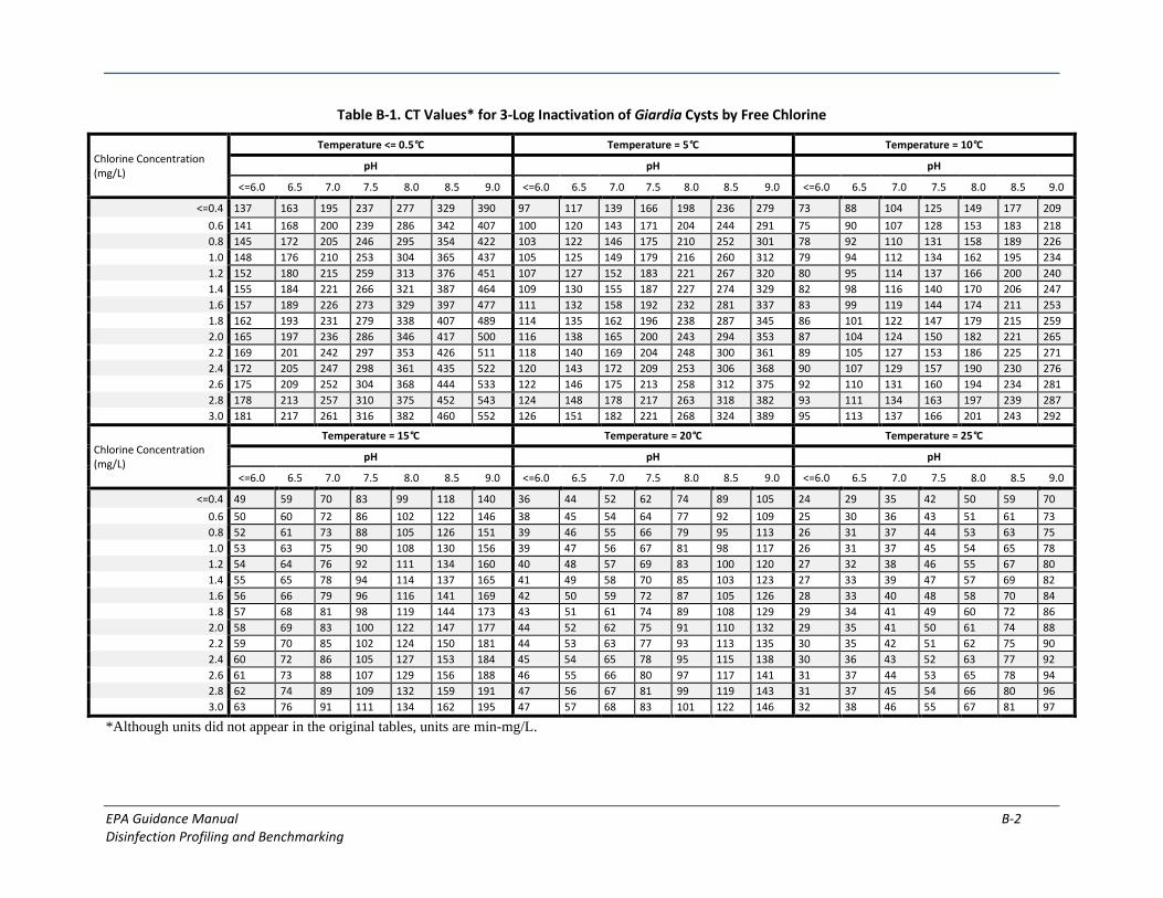
EPA Guidance Manual B-2Disinfection Profiling and Benchmarking
Table B-1. CT Values* for 3-Log Inactivation of Giardia Cysts by Free Chlorine
Chlorine Concentration (mg/L)
Temperature <= 0.5°C Temperature = 5°C Temperature = 10°C
pH pH pH
<=6.0 6.5 7.0 7.5 8.0 8.5 9.0 <=6.0 6.5 7.0 7.5 8.0 8.5 9.0 <=6.0 6.5 7.0 7.5 8.0 8.5 9.0
<=0.4 137 163 195 237 277 329 390 97 117 139 166 198 236 279 73 88 104 125 149 177 209 0.6 141 168 200 239 286 342 407 100 120 143 171 204 244 291 75 90 107 128 153 183 218 0.8 145 172 205 246 295 354 422 103 122 146 175 210 252 301 78 92 110 131 158 189 226 1.0 148 176 210 253 304 365 437 105 125 149 179 216 260 312 79 94 112 134 162 195 234 1.2 152 180 215 259 313 376 451 107 127 152 183 221 267 320 80 95 114 137 166 200 240 1.4 155 184 221 266 321 387 464 109 130 155 187 227 274 329 82 98 116 140 170 206 247 1.6 157 189 226 273 329 397 477 111 132 158 192 232 281 337 83 99 119 144 174 211 253 1.8 162 193 231 279 338 407 489 114 135 162 196 238 287 345 86 101 122 147 179 215 259 2.0 165 197 236 286 346 417 500 116 138 165 200 243 294 353 87 104 124 150 182 221 265 2.2 169 201 242 297 353 426 511 118 140 169 204 248 300 361 89 105 127 153 186 225 271 2.4 172 205 247 298 361 435 522 120 143 172 209 253 306 368 90 107 129 157 190 230 276 2.6 175 209 252 304 368 444 533 122 146 175 213 258 312 375 92 110 131 160 194 234 281 2.8 178 213 257 310 375 452 543 124 148 178 217 263 318 382 93 111 134 163 197 239 287 3.0 181 217 261 316 382 460 552 126 151 182 221 268 324 389 95 113 137 166 201 243 292
Chlorine Concentration (mg/L)
Temperature = 15°C Temperature = 20°C Temperature = 25°C
pH pH pH
<=6.0 6.5 7.0 7.5 8.0 8.5 9.0 <=6.0 6.5 7.0 7.5 8.0 8.5 9.0 <=6.0 6.5 7.0 7.5 8.0 8.5 9.0
<=0.4 0.6 0.8 1.0 1.2 1.4 1.6 1.8 2.0 2.2 2.4 2.6 2.8 3.0
49 59 70 83 99 118 140 36 44 52 62 74 89 105 24 29 35 42 50 59 70 50 60 72 86 102 122 146 38 45 54 64 77 92 109 25 30 36 43 51 61 73 52 61 73 88 105 126 151 39 46 55 66 79 95 113 26 31 37 44 53 63 75 53 63 75 90 108 130 156 39 47 56 67 81 98 117 26 31 37 45 54 65 78 54 64 76 92 111 134 160 40 48 57 69 83 100 120 27 32 38 46 55 67 80 55 65 78 94 114 137 165 41 49 58 70 85 103 123 27 33 39 47 57 69 82 56 66 79 96 116 141 169 42 50 59 72 87 105 126 28 33 40 48 58 70 84 57 68 81 98 119 144 173 43 51 61 74 89 108 129 29 34 41 49 60 72 86 58 69 83 100 122 147 177 44 52 62 75 91 110 132 29 35 41 50 61 74 88 59 70 85 102 124 150 181 44 53 63 77 93 113 135 30 35 42 51 62 75 90 60 72 86 105 127 153 184 45 54 65 78 95 115 138 30 36 43 52 63 77 92 61 73 88 107 129 156 188 46 55 66 80 97 117 141 31 37 44 53 65 78 94 62 74 89 109 132 159 191 47 56 67 81 99 119 143 31 37 45 54 66 80 96 63 76 91 111 134 162 195 47 57 68 83 101 122 146 32 38 46 55 67 81 97
*Although units did not appear in the original tables, units are min-mg/L.

EPA Guidance Manual B-3 Disinfection Profiling and Benchmarking
Table B-2. CT Values* for 4-Log Inactivation of Viruses by Free Chlorine
pH
Temperature (°C) 6-9 10
0.5 12 90
5 8 60
10 6 45
15 4 30
20 3 22
25 2 15 *Although units did not appear in the original tables, units are min-mg/L.
Table B-3. CT Values* for 3-Log Inactivation of Giardia Cysts by Chlorine Dioxide
Temperature (°C)
< = 1 5 10 15 20 25
63 26 23 19 15 11 *Although units did not appear in the original tables, units are min-mg/L.
Table B-4. CT Values* for 4-Log Inactivation of Viruses by Chlorine Dioxide pH 6-9
Temperature (°C)
< = 1 5 10 15 20 25
50.1 33.4 25.1 16.7 12.5 8.4 *Although units did not appear in the original tables, units are min-mg/L.
Table B-5. CT Values* for 3-Log Inactivation of Giardia Cysts by Ozone
Temperature (°C)
< = 1 5 10 15 20 25
2.9 1.90 1.43 0.95 0.72 0.48 *Although units did not appear in the original tables, units are min-mg/L.

EPA Guidance Manual B-4 Disinfection Profiling and Benchmarking
Table B-6. CT Values* for 4-Log Inactivation of Viruses by Ozone
Temperature (°C)
< = 1 5 10 15 20 25
1.8 1.2 1.0 0.6 0.5 0.3 *Although units did not appear in the original tables, units are min-mg/L.
Table B-7. CT Values* for 3-Log Inactivation of Giardia Cysts by Chloramines^ pH 6-9
Temperature (°C)
< = 1 5 10 15 20 25
3,800 2,200 1,850 1,500 1,100 750 *Although units did not appear in the original tables, units are min-mg/L. ^It is assumed that Chlorine is used as primary and Ammonia as secondary disinfectant to form Chloramines for disinfection (See Section 8.2.1).
Table B-8. CT Values* for 4-Log Inactivation of Viruses by Chloramines^
Temperature (°C)
< = 1 5 10 15 20 25
2,883 1,988 1,491 994 746 497 *Although units did not appear in the original tables, units are min-mg/L. ^It is assumed that Chlorine is used as primary and Ammonia as secondary disinfectant to form Chloramines for disinfection (See Section 8.2.1).
Table B-9. UV Dose Table for Cryptosporidium, Giardia, and Virus Inactivation Credit (USEPA, April 2010)
Log credit Cryptosporidium UV dose (mJ/cm2)
Giardia lamblia UV dose (mJ/cm2)
Virus UV dose (mJ/cm2)
0.5 1.6 1.5 39
1.0 2.5 2.1 58
1.5 3.9 3.0 79
2.0 5.8 5.2 100
2.5 8.5 7.7 121
3.0 12 11 143
3.5 15 15 163
4.0 22 22 186

EPA Guidance Manual B-5 Disinfection Profiling and Benchmarking
References
USEPA. July 2002. Code of Federal Regulations, Title 40, Chapter I, Section 141.2.
USEPA. April 2010. Long Term 2 Enhanced Surface Water Treatment Rule Toolbox Guidance Manual. EPA 815-R-09-016. Washington, D.C.

EPA Guidance Manual B-6 Disinfection Profiling and Benchmarking
This Page Intentionally Left Blank

EPA Guidance Manual C-1 Disinfection Profiling and Benchmarking
Appendix C — Blank Worksheets This appendix contains worksheets that can be used to record operational information on disinfection processes used for pathogen inactivation. A public water system (PWS) should confirm reporting requirements with its state prior to using these worksheets for compliance purposes. Examples using these worksheets are presented in Chapters 3 through 5 and Appendix D.
Worksheet #1 applies to PWSs with surface water or GWUDI sources of supply that use chemical disinfectants for pathogen inactivation. Worksheet #1 can be used to record weekly water quality and operational data needed to determine actual CT, required CT, and the pathogen inactivation credit.
Worksheet #2 applies to surface water and GWUDI systems using multiple segments of chemical disinfectants. Worksheet #2 can be used to add the inactivation ratios for each disinfection segment to calculate the total pathogen inactivation credit.
Worksheets #3, 4, 5, and 6 apply to PWSs using UV disinfection for pathogen inactivation. Systems using UV disinfection have different reporting requirements than systems using chemical disinfectants because pathogen inactivation is documented based on the UV dosage rate and not based on a CT value. The LT2ESWTR requires PWSs to report the following items to the state for UV disinfection:
• Initial reporting – Validation test results demonstrating operating conditions that achieve the UV dose required for compliance with the LT2ESWTR (See Worksheet #3).
• Routine reporting – Percentage of water entering the distribution system that was not treated by the UV reactors operating within validated conditions on a monthly basis (See Worksheets #4 and #5).
• Additional UV calculation worksheet – Worksheet #6 does not need to be submitted to the state. It is used to calculate the daily off-specification volume (i.e., the daily volume of water disinfected using UV components that are not equal to or better than installed UV components that have been properly validated). The daily off-specification volume is recorded on Worksheets #4 and #5. Note that Worksheets #4 and #5 refer to this worksheet as Figure 6.5 which is the figure number used in the UV Guidance Manual (USEPA, November 2006).

EPA Guidance Manual C-2 Disinfection Profiling and Benchmarking
Starting Month: Year: PWSID: System/Water Source:
Disinfectant Type: ________________ Prepared by:Profile Type (check one): Giardia Viruses
Disinfection Segment/Sequence of Application:
3 4 5 6 7 8 9 10 11 12 13 14Residual Peak Disinf.Disinf. pH Water Hourly TDT Baffling Contact CTCalc = CT Inactivation Log
Week Conc. Temp. Flow Volume Factor Time (CxT) Req'd Ratio Inactivation*# C (mg/L) (oC) (gpm) (gal) (min.) T (min.) (min-mg/L) (min-mg/L) (Col 11 / Col 12)12345678910111213141516171819202122232425262728293031323334353637383940414243444546474849505152
*See worksheet #2 to determine total log inactivation if the system has multiple disinfection segments.
ACTIVATION RATIO DETERMINATION FOR SURFACE WATER LOG IN SYSTEMS ORGROUND WATER SYSTEMS UNDER THE DIRECT INFLUENCE OF SURFACE WATER
WORKSHEET #1

EPA Guidance Manual C-3 Disinfection Profiling and Benchmarking
Notes:
1. The PWS is only required to calculate log inactivation values once per week on the same day of the week. For instance, the PWS may choose to calculate log inactivation values on Wednesday of every week. If the PWS has more than one point of disinfectant application or uses more than one type of disinfectant, then the PWS can calculate log inactivation ratios on separate sheets and sum the log inactivation ratios to obtain the total inactivation achieved by the plant using Worksheet #2 in this Appendix.
2. Use a separate form for each disinfectant application point and related residual sample site. Enter the disinfectant and sequence position, e.g., "ozone/1st" or "chlorine dioxide/3rd".
3. Residual disinfectant concentration must be measured during peak hourly flow.
4. If the PWS uses chlorine, the pH of the disinfected water must be measured at the same location and time the chlorine residual disinfectant concentration is measured during peak hourly flow.
5. The water temperature must be measured at the same location and time the residual disinfectant concentration is measured during peak hourly flow. Temperature must be in degrees Celsius (°C).
6. Peak hourly flow for the day must be provided for the disinfection segment.
7. The volume is the operating volume in gallons realized by the pipe, basin, or treatment unit process during peak hourly flow.
8. Theoretical detention time in minutes equals the volume in gallons (in column 7) divided by the peak hourly flow in gpm (in column 6).
9. Enter the baffling factor for the PWS's pipe, basin(s) or treatment unit process as determined by a tracer study or assigned by the state.
10. Disinfectant contact time in minutes is determined by multiplying the theoretical detention time in minutes in column 8 by the baffling factor in column 9.
11. CTcalc is determined by multiplying the residual disinfectant concentration in mg/L in column 3 by the disinfectant contact time in minutes in column 10.
12. The CTrequired value should be determined based on the tables contained in Appendix B or tables in the USEPA Guidance Manual for Compliance with the Filtration and Disinfection Requirements for Public Water Systems Using Surface Water (USEPA, March 1991). CTrequired for Giardia is CT99.9 (or 3-log inactivation) and CTrequired for viruses is CT99.99 (or 4-log inactivation).
13. Inactivation ratio equals CTcalc in column 11 divided by CTrequired in column 12.
14. Log Inactivation for Giardia = 3 x Inactivation ratio in column 13. Log Inactivation for viruses = 4 x Inactivation ratio in column 13.
For multiple disinfection segments, Worksheet #2 should be used to sum inactivation ratios for each disinfection segment to calculate log inactivation.
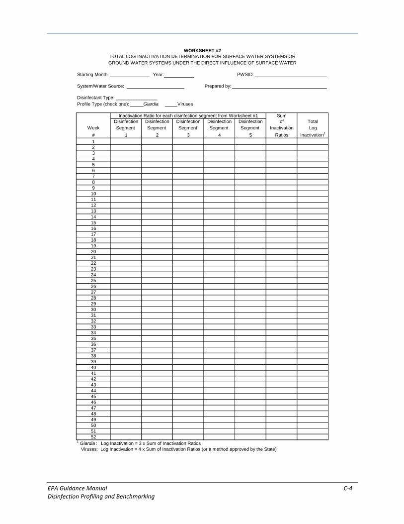
EPA Guidance Manual C-4 Disinfection Profiling and Benchmarking
Starting Month: Year: PWSID:
System/Water Source: Prepared by:
Disinfectant Type: ________________Profile Type (check one): Giardia Viruses
SumDisinfection Disinfection Disinfection Disinfection Disinfection of Total
Week Segment Segment Segment Segment Segment Inactivation Log# 1 2 3 4 5 Ratios Inactivation1
12345678910111213141516171819202122232425262728293031323334353637383940414243444546474849505152
1 Giardia : Log Inactivation = 3 x Sum of Inactivation Ratios Viruses: Log Inactivation = 4 x Sum of Inactivation Ratios (or a method approved by the State)
Inactivation Ratio for each disinfection segment from Worksheet #1
TOTAL LOG INACTIVATION DETERMINATION FOR SURFACE WATER SYSTEMS ORGROUND WATER SYSTEMS UNDER THE DIRECT INFLUENCE OF SURFACE WATER
WORKSHEET #2
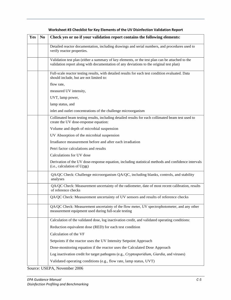
EPA Guidance Manual C-5 Disinfection Profiling and Benchmarking
Worksheet #3 Checklist for Key Elements of the UV Disinfection Validation Report
Yes No Check yes or no if your validation report contains the following elements:
Detailed reactor documentation, including drawings and serial numbers, and procedures used to verify reactor properties.
Validation test plan (either a summary of key elements, or the test plan can be attached to the validation report along with documentation of any deviations to the original test plan)
Full-scale reactor testing results, with detailed results for each test condition evaluated. Data should include, but are not limited to:
flow rate,
measured UV intensity,
UVT, lamp power,
lamp status, and
inlet and outlet concentrations of the challenge microorganism
Collimated beam testing results, including detailed results for each collimated beam test used to create the UV dose-response equation:
Volume and depth of microbial suspension
UV Absorption of the microbial suspension
Irradiance measurement before and after each irradiation
Petri factor calculations and results
Calculations for UV dose
Derivation of the UV dose-response equation, including statistical methods and confidence intervals (i.e., calculation of UDR)
QA/QC Check: Challenge microorganism QA/QC, including blanks, controls, and stability analyses
QA/QC Check: Measurement uncertainty of the radiometer, date of most recent calibration, results of reference checks
QA/QC Check: Measurement uncertainty of UV sensors and results of reference checks
QA/QC Check: Measurement uncertainty of the flow meter, UV spectrophotometer, and any other measurement equipment used during full-scale testing
Calculation of the validated dose, log inactivation credit, and validated operating conditions:
Reduction equivalent dose (RED) for each test condition
Calculation of the VF
Setpoints if the reactor uses the UV Intensity Setpoint Approach
Dose-monitoring equation if the reactor uses the Calculated Dose Approach
Log inactivation credit for target pathogens (e.g., Cryptosporidium, Giardia, and viruses)
Validated operating conditions (e.g., flow rate, lamp status, UVT)
Source: USEPA, November 2006

EPA Guidance Manual C-6 Disinfection Profiling and Benchmarking
Worksheet #4 Example Daily Operating Log for Calculated Dose Approach
Source: USEPA, November 2006

EPA Guidance Manual C-7 Disinfection Profiling and Benchmarking
Worksheet #5 Example Daily Operating Log for UV Intensity Setpoint Approach
Source: USEPA, November 2006

EPA Guidance Manual C-8 Disinfection Profiling and Benchmarking
Worksheet #6 Example Off-specification Calculation Worksheet
Source: USEPA, November 2006
EPA Guidance Manual C-9 Disinfection Profiling and Benchmarking
References
USEPA. March 1991. Guidance Manual for Compliance with the Filtration and Disinfection Requirements for Public Water Systems Using Surface Water. Washington, D.C.
USEPA. November 2006. Ultraviolet Disinfection Guidance Manual for the Final Long Term 2 Enhanced Surface Water Treatment Rule. EPA 815-R-06-006. Washington, D.C.

EPA Guidance Manual C-10 Disinfection Profiling and Benchmarking
This Page Intentionally Left Blank

EPA Guidance Manual D-1 Disinfection Profiling and Benchmarking
Appendix D — Examples This appendix provides three examples of ways a PWS may comply with the regulations for a disinfection profile and a disinfection benchmark. This appendix does not establish any additional requirements for completing a disinfection profile or a disinfection benchmark beyond the regulations established in the LT2ESWTR, LT1ESWTR, and IESWTR.
The following examples are presented in this appendix:
• Example D-1: Calculate Log Inactivation for One Disinfection Segment and One Disinfectant (Chlorine)
• Example D-2: Calculate Log Inactivation for Three Disinfection Segments and Two Disinfectants (Chlorine as primary and Chloramines as secondary disinfectant)
• Example D-3: Develop a Disinfection Profile and Benchmark for a PWS with Multiple Disinfection Segments and Two Disinfectants (Ozone as primary and Chlorine as secondary disinfectant)
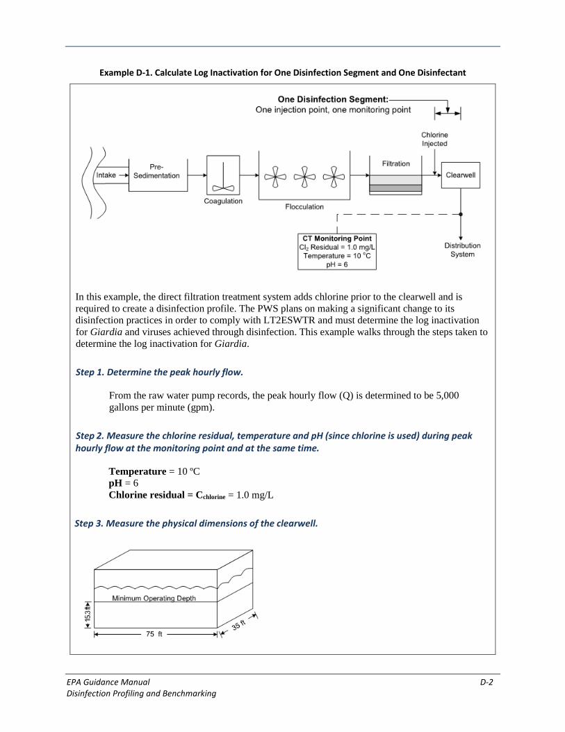
EPA Guidance Manual D-2Disinfection Profiling and Benchmarking
Example D-1. Calculate Log Inactivation for One Disinfection Segment and One Disinfectant
In this example, the direct filtration treatment system adds chlorine prior to the clearwell and is required to create a disinfection profile. The PWS plans on making a significant change to its disinfection practices in order to comply with LT2ESWTR and must determine the log inactivation for Giardia and viruses achieved through disinfection. This example walks through the steps taken to determine the log inactivation for Giardia.
Step 1. Determine the peak hourly flow.
From the raw water pump records, the peak hourly flow (Q) is determined to be 5,000 gallons per minute (gpm).
Step 2. Measure the chlorine residual, temperature and pH (since chlorine is used) during peak hourly flow at the monitoring point and at the same time.
Temperature = 10 ºC pH = 6 Chlorine residual = Cchlorine = 1.0 mg/L
Step 3. Measure the physical dimensions of the clearwell.

EPA Guidance Manual D-3Disinfection Profiling and Benchmarking
Measure the inner tank length and width to obtain the area of the clearwell.
Length = 75 ft
Width = 35 ft
Measure the minimum operating depth in the clearwell to obtain a conservative estimate of the volume of water in the tank.
Minimum Operating Depth = 15.3 ft
Step 4. Calculate the volume of the water in the clearwell based on low water level.
Volume (V) = minimum water depth x length x width V = 15.3 ft x 75 ft x 35 ft = 40,160 ft3 V = 40,160 ft3 x (7.48 gal / ft3) V = 300,000 gal
Step 5. Calculate the Theoretical Detention Time (TDT) in the clearwell.
TDT = V / Q (Note: Q = peak hourly flow) TDT = 300,000 gal / 5,000 gpm TDT = 60 minutes
Step 6. Determine the baffling factor (BF) for the clearwell.
Clearwell BF = 0.5 (from Table G-1 in Appendix G for average baffling condition as shown below.)
Step 7. Calculate the contact time of the disinfectant in the clearwell.
Contact Time (T) = TDT x BF T = 60 min x 0.5 T = 30 minutes

EPA Guidance Manual D-4 Disinfection Profiling and Benchmarking
Step 8. Calculate the CT for the disinfection segment.
CTcalc = Cchlorine x T CTcalc = 1.0 mg/L x 30 min CTcalc = 30 min-mg/L
Step 9. Determine the required CT99.9 necessary to obtain 3-log Giardia inactivation.
The required CT value for 3-log Giardia inactivation (CT99.9) may be obtained by using CT Table B-1 in Appendix B, CT Values for 3-Log Inactivation of Giardia Cysts by Free Chlorine. In this example, the required CT99.9 is 79 min-mg/L for a pH of 6, temperature of 10°C, and Cchlorine of 1.0 mg/L. The relevant section of Table B-1 is reprinted below and the pertinent section of the table is highlighted.
Excerpt from Table B-1
CT Values for 3-Log Inactivation of Giardia Cysts by Free Chlorine (10°C portion of table, for concentrations from 0.4 to 1.2)
Chlorine Concentration
(mg/L)
Temperature = 10°C
pH
<=6.0 6.5 7.0 7.5 8.0 8.5 9.0
<=0.4 73 88 104 125 149 177 209
0.6 75 90 107 128 153 183 218
0.8 78 92 110 131 158 189 226
1.0 79 94 112 134 162 195 234
1.2 80 95 114 137 166 200 240
Step 10. Calculate the inactivation ratio for the clearwell.
Inactivation ratio = CTcalc / CT99.9 = (30 min-mg/L) / (79 min-mg/L)
Inactivation ratio = 0.380
Step 11. Calculate the Giardia log inactivation for the clearwell.
Log inactivation = 3 x CTcalc / CT99.9 Log inactivation = 3 x 0.380 Log inactivation = 1.14
The Giardia log inactivation for this disinfection segment is 1.14.
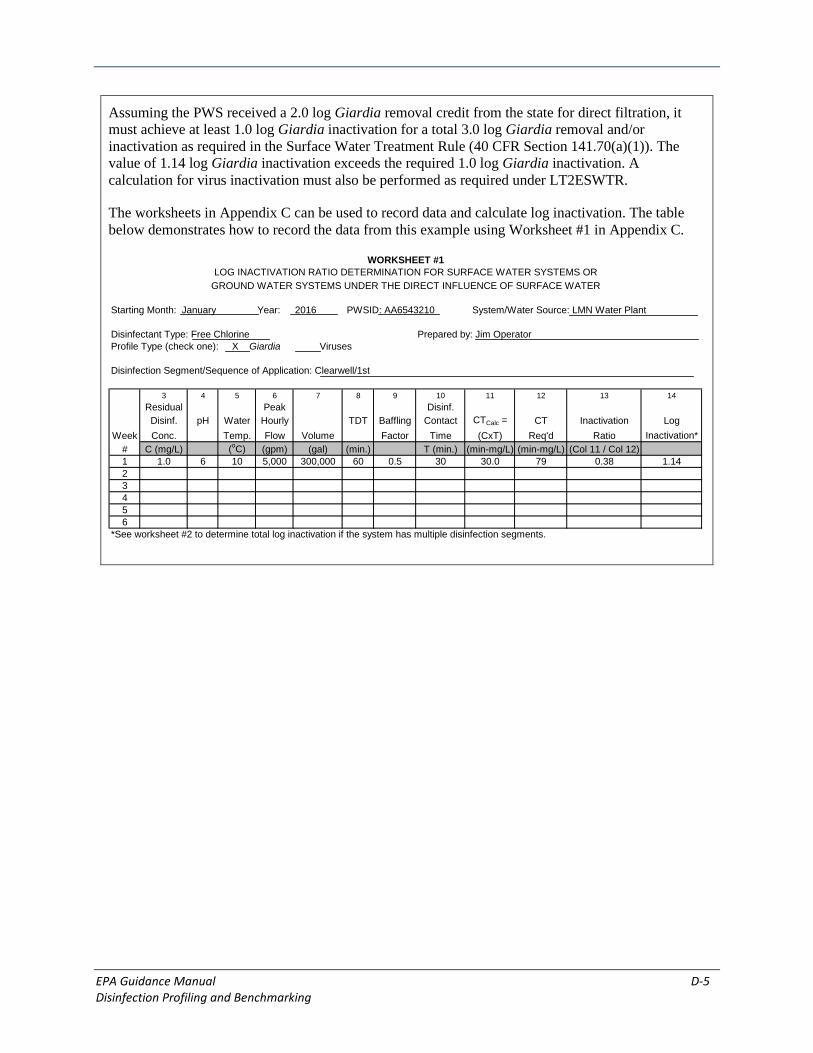
EPA Guidance Manual D-5 Disinfection Profiling and Benchmarking
Assuming the PWS received a 2.0 log Giardia removal credit from the state for direct filtration, it must achieve at least 1.0 log Giardia inactivation for a total 3.0 log Giardia removal and/or inactivation as required in the Surface Water Treatment Rule (40 CFR Section 141.70(a)(1)). The value of 1.14 log Giardia inactivation exceeds the required 1.0 log Giardia inactivation. A calculation for virus inactivation must also be performed as required under LT2ESWTR.
The worksheets in Appendix C can be used to record data and calculate log inactivation. The table below demonstrates how to record the data from this example using Worksheet #1 in Appendix C.
Starting Month: January Year: 2016 PWSID: AA6543210 System/Water Source: LMN Water Plant
Disinfectant Type: Free Chlorine Prepared by: Jim OperatorProfile Type (check one): X Giardia Viruses
Disinfection Segment/Sequence of Application: Clearwell/1st
3 4 5 6 7 8 9 10 11 12 13 14Residual Peak Disinf.Disinf. pH Water Hourly TDT Baffling Contact CTCalc = CT Inactivation Log
Week Conc. Temp. Flow Volume Factor Time (CxT) Req'd Ratio Inactivation*# C (mg/L) (oC) (gpm) (gal) (min.) T (min.) (min-mg/L) (min-mg/L) (Col 11 / Col 12)1 1.0 6 10 5,000 300,000 60 0.5 30 30.0 79 0.38 1.1423456
*See worksheet #2 to determine total log inactivation if the system has multiple disinfection segments.
WORKSHEET #1LOG INACTIVATION RATIO DETERMINATION FOR SURFACE WATER SYSTEMS OR
GROUND WATER SYSTEMS UNDER THE DIRECT INFLUENCE OF SURFACE WATER

EPA Guidance Manual D-6 Disinfection Profiling and Benchmarking
Example D-2. Calculate Log Inactivation for Three Disinfection Segments and Two Disinfectants
In this example, chlorine is added to the conventional treatment system before coagulation as a pre-disinfectant and again prior to the clearwell as a primary disinfectant. Ammonia is added after the clearwell to create chloramines as the secondary disinfectant to maintain a residual throughout the distribution system. The PWS is considering changes to their disinfection practices. Therefore, under LT2ESWTR, the PWS is required to create a disinfection profile and benchmark and consult with the state. For the profile, the PWS is required to calculate the log inactivation for Giardia and viruses. This example walks through the steps taken to determine the log inactivation for Giardia.
Since there are three points where the disinfectant is added, the inactivation ratio must be calculated for each disinfection segment.
A. Determine the Giardia Inactivation Ratio for Disinfection Segment 1
Disinfection Segment 1 begins at the chlorine injection location just prior to coagulation and ends at the chlorine monitoring point just after the filters.
Step 1. Determine the peak hourly flow.
From the raw water pump records the peak hourly flow (Q) is determined to be 5,000 gpm.
Step 2. Measure the chlorine residual, temperature and pH (since chlorine is used) during peak hourly flow at the chlorine monitoring point and at the same time.
Temperature = 10ºC pH = 7.5 Chlorine residual = Cchlorine = 1.0 mg/L

EPA Guidance Manual D-7 Disinfection Profiling and Benchmarking
Step 3. Measure the physical dimensions of the sub-units in Disinfection Segment 1.
Measure inner tank diameter or length and width to obtain the area of water in the tanks rather than the area of the tanks themselves.
Measure the minimum operating depth in the tanks, where applicable, to obtain conservative estimates of the volume of water in the tanks.
Coagulation:
Length = 13.7 ft Width = 13.7 ft Depth = 17.1 ft
Flocculation:
Length = 66.4 ft Width = 11.5 ft Depth = 14.0 ft
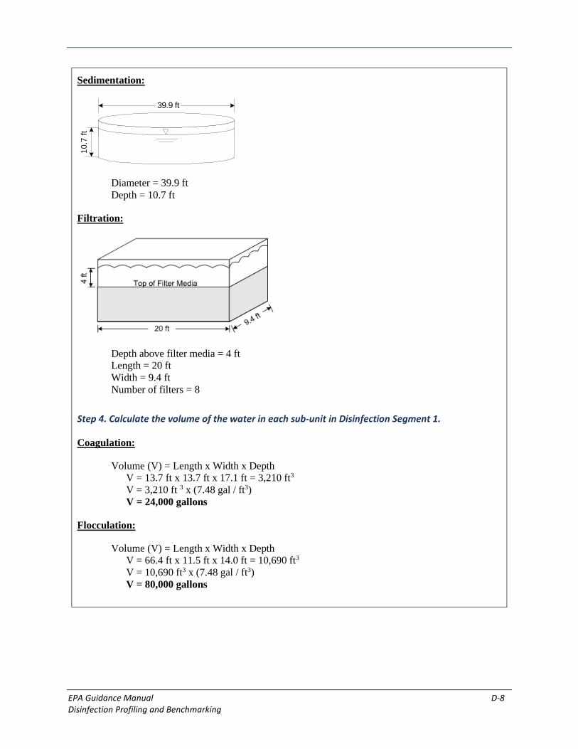
EPA Guidance Manual D-8 Disinfection Profiling and Benchmarking
Sedimentation:
39.9 ft
10.7
ft
Diameter = 39.9 ft Depth = 10.7 ft
Filtration:
Depth above filter media = 4 ft Length = 20 ft Width = 9.4 ft Number of filters = 8
Step 4. Calculate the volume of the water in each sub-unit in Disinfection Segment 1.
Coagulation:
Volume (V) = Length x Width x Depth V = 13.7 ft x 13.7 ft x 17.1 ft = 3,210 ft3 V = 3,210 ft 3 x (7.48 gal / ft3) V = 24,000 gallons
Flocculation:
Volume (V) = Length x Width x Depth V = 66.4 ft x 11.5 ft x 14.0 ft = 10,690 ft3 V = 10,690 ft3 x (7.48 gal / ft3) V = 80,000 gallons

EPA Guidance Manual D-9 Disinfection Profiling and Benchmarking
Sedimentation:
Volume (V) = π x Radius2 x Depth π = 3.14 (constant)
Radius = Diameter / 2 = 39.9 / 2 = 19.95 ft V = 3.14 x (19.95 ft)2 x 10.7 ft = 13,370 ft3 V = 13,370 ft3 x (7.48 gal / ft3) V = 100,000 gallons
Filtration:
Volume (V) = Length x Width x Depth of Water Above Media x # of Filters V = 20 ft x 9.4 ft x 4 ft x 8 filters = 6,020 ft3 V = 6,020 ft3 x (7.48 gal / ft3) V = 45,000 gallons
Step 5. Calculate the Theoretical Detention Time (TDT) in the sub-units in Disinfection Segment 1.
TDT = V / Q
Coagulation:
TDT = 24,000 gal / 5,000 gpm TDT = 4.8 minutes
Flocculation:
TDT = 80,000 gal / 5,000 gpm TDT = 16 minutes
Sedimentation:
TDT = 100,000 gal / 5,000 gpm TDT = 20 minutes
Filtration:
TDT = 45,000 gal / 5,000 gpm TDT = 9 minutes

EPA Guidance Manual D-10 Disinfection Profiling and Benchmarking
Step 6. Determine the baffling factors (BF) for the sub-units in Disinfection Segment 1.
The table below summarizes the baffling factors in this example for the sub-units in Disinfection Segment 1.
Unit Process BF *
(1) Coagulation 0.1
(2) Flocculation 0.1
(3) Sedimentation 0.5
(4) Filtration 0.7 *See Appendix G for Baffling Factors
Step 7. Calculate the contact time (T) in the sub-units in Disinfection Segment 1.
T = TDT x BF
Coagulation:
T = 4.8 min x 0.1 T = 0.48 minutes
Flocculation:
T = 16 min x 0.1 T = 1.6 minutes
Sedimentation:
T = 20 min x 0.5 T = 10 minutes
Filtration:
T = 9 min x 0.7 T = 6.3 minutes
Step 8. Calculate the total contact time in Disinfection Segment 1.
Total Contact Time (Ttotal) = Sum of T in each sub-unit Ttotal = 0.48 min + 1.6 min + 10 min + 6.3 min Ttotal = 18.4 minutes

EPA Guidance Manual D-11 Disinfection Profiling and Benchmarking
Step 9. Calculate the CT for Disinfection Segment 1 (CTcalc)
CTcalc = Cchlorine x Ttotal CTcalc = 1.0 mg/L x 18.4 min CTcalc = 18.4 min-mg/L
The CTcalc for Disinfection Segment 1 = 18.4 min-mg/L
Step 10. Determine the required CT99.9 necessary to obtain 3-log Giardia inactivation.
The required CT value for 3-log Giardia inactivation (CT99.9) may be obtained by using CT Table B-1 in Appendix B, CT Values for 3-Log Inactivation of Giardia Cysts by Free Chlorine. The CT99.9 in this example is 134 min-mg/L for a pH of 7.5, temperature of 10°C, and Cchlorine of 1.0 mg/L. The relevant section of Table B-1 is reprinted below and the pertinent section of the table is highlighted.
Excerpt from Table B-1
CT Values for 3-Log Inactivation of Giardia Cysts by Free Chlorine (10°C portion of table, for concentrations from 0.6 to 1.4)
Chlorine Concentration
(mg/L)
Temperature = 10°C
pH
<=6.0 6.5 7.0 7.5 8.0 8.5 9.0
0.6 75 90 107 128 153 183 218
0.8 78 92 110 131 158 189 226
1.0 79 94 112 134 162 195 234
1.2 80 95 114 137 166 200 240
1.4 82 98 116 140 170 206 247
Step 11. Calculate the inactivation ratio for Disinfection Segment 1.
Inactivation ratio = CTcalc / CT99.9 Inactivation ratio = (18.4 min-mg/L) / (134 min-mg/L) Inactivation ratio = 0.137
B. Determine the Giardia Inactivation Ratio for Disinfection Segment 2
Disinfection Segment 2 in this example begins at the chlorine injection location just prior to the clearwell and ends just after the clearwell.

EPA Guidance Manual D-12 Disinfection Profiling and Benchmarking
Step 1. Determine the peak hourly flow.
The peak hourly flow (Q) for Disinfection Segment 2 is the same as the peak hourly flow in Disinfection Segment 1.
Peak hourly flow = 5,000 gpm.
Step 2. Measure the chlorine residual, temperature, and pH (since chlorine is used) during peak hourly flow at the chlorine monitoring point and at the same time.
Temperature = 10ºC Chlorine residual = Cchlorine = 1.2 mg/L pH = 7.5
Step 3. Measure the physical dimensions of the clearwell.
Measure the inner tank length and width to obtain the volume of water in the clearwell rather than the volume of the tank itself.
Length = 75 ft Width = 35 ft
Measure the minimum operating depth in the clearwell to obtain a conservative estimate of the volume of water in the tank.
Minimum Operating Depth = 15.3 ft
Step 4. Calculate the volume of the water in the clearwell based on low water level.
Volume (V) = minimum water depth x length x width V = 15.3 ft x 75 ft x 35 ft = 40,160 ft3 V = 40,160 ft3 x (7.48 gal / ft3) V= 300,000 gal

EPA Guidance Manual D-13 Disinfection Profiling and Benchmarking
Step 5. Calculate the Theoretical Detention Time in the clearwell.
Theoretical Detention Time (TDT) = V / Q TDT = 300,000 gal / 5,000 gpm TDT = 60 minutes
Step 6. Determine the baffling factor for the clearwell.
Clearwell Baffling Factor (BF) = 0.7 (from Table G-1 for superior baffling condition as shown below.)
Step 7. Calculate the contact time of the disinfectant in the clearwell.
Contact Time (T) = TDT x BF T = 60 min x 0.7 T = 42 minutes
Step 8. Calculate the CT for the disinfection segment.
CTcalc = Cchlorine x T CTcalc = 1.2 mg/L x 42 min CTcalc = 50 min-mg/L

EPA Guidance Manual D-14 Disinfection Profiling and Benchmarking
Step 9. Determine the required CT99.9 necessary to obtain 3-log Giardia inactivation.
The required CT value for 3-log Giardia inactivation (CT99.9) may be obtained by using CT Table B-1 in Appendix B, CT Values for 3-Log Inactivation of Giardia Cysts by Free Chlorine. The CT99.9 in this example is 137 min-mg/L for a pH of 7.5, temperature of 10°C, and Cchlorine of 1.2 mg/L. The relevant section of Table B-1 is reprinted below and the pertinent section of the table is highlighted.
Excerpt from Table B-1
CT Values for 3-Log Inactivation of Giardia Cysts by Free Chlorine (10°C portion of table, for concentrations from 0.8 to 1.6)
Chlorine Concentration
(mg/L)
Temperature = 10°C
pH
<=6.0 6.5 7.0 7.5 8.0 8.5 9.0
0.8 78 92 110 131 158 189 226
1.0 79 94 112 134 162 195 234
1.2 80 95 114 137 166 200 240
1.4 82 98 116 140 170 206 247
1.6 83 99 119 144 174 211 253
Step 10. Calculate the inactivation ratio for the clearwell.
Inactivation ratio = CTcalc / CT99.9 Inactivation ratio = (50 min-mg/L) / (137 min-mg/L) Inactivation ratio = 0.365
C. Determine the Giardia Inactivation Ratio for Disinfection Segment 3
Disinfection Segment 3 in this example begins at the chloramine injection location after the clearwell and ends at the monitoring point in the transmission pipe, which is prior to the first customer.
Step 1. Determine the peak hourly flow.
The peak hourly flow (Q) for Disinfection Segment 3 is the same as the peak hourly flow in Disinfection Segments 1 and 2.
Peak hourly flow = 5,000 gpm

EPA Guidance Manual D-15 Disinfection Profiling and Benchmarking
Step 2. Measure the chloramine residual and temperature during peak hourly flow at the chlorine monitoring point and at the same time.
Temperature = 10ºC Chloramine residual = Cchloramine = 0.6 mg/L
Step 3. Measure the physical dimensions of the pipe.
5,280 Feet
Side View
End View(Closeup)
Diameter = 12 in
Measure the length of the pipe and the inner pipe diameter to obtain the volume of water in the pipe rather than the volume of the pipe itself.
Diameter = 12 in x (1 ft / 12 in) = 1 ft Length = 5,280 ft
Step 4. Calculate the volume of the water in the pipe.
Volume (V) = π x Radius2 x Length π = 3.14 (constant)
Radius = Diameter / 2 = 1.0 / 2 = 0.5 ft V = 3.14 x (0.5 ft)2 x 5,280 ft = 4,145 ft3 V= 4,145 ft3 x (7.48 gal / ft3) V = 31,000 gallons
Step 5. Calculate the Theoretical Detention Time in the pipe.
Theoretical Detention Time (TDT) = V / Q TDT = 31,000 gal / 5,000 gpm TDT = 6.2 minutes

EPA Guidance Manual D-16 Disinfection Profiling and Benchmarking
Step 6. Determine the baffling factor for the pipe.
Baffling Factor (BF) = 1.0 (from Table G-1 in Appendix G for a pipe)
Step 7. Calculate the contact time of the disinfectant in the pipe.
Contact Time (T) = TDT x BF T = 6.2 min x 1.0 T = 6.2 minutes
Step 8. Calculate the CT for the disinfection segment.
CTcalc = Cchloramine x T CTcalc = 0.6 mg/L x 6.2 min CTcalc = 3.7 min-mg/L
Step 9. Determine the required CT99.9 necessary to obtain 3-log Giardia inactivation.
The required CT value for 3-log Giardia inactivation (CT99.9) may be obtained by using CT Table B-7 in Appendix B, CT Values for 3-Log Inactivation of Giardia Cysts by Chloramine pH 6-9. The CT99.9 in this example is 1,850 min-mg/L for a temperature of 10°C. Table B-7 is reprinted below and the pertinent section of the table is highlighted.
Table B-7
CT Values for 3-Log Inactivation of Giardia Cysts by Chloramine pH 6-9
Temperature (°C)
< = 1 5 10 15 20 25
3,800 2,200 1,850 1,500 1,100 750
Step 10. Calculate the inactivation ratio for the pipe.
Inactivation ratio = CTcalc / CT99.9 Inactivation ratio = (3.7 min-mg/L) / (1,850 min-mg/L) Inactivation ratio = 0.002

EPA Guidance Manual D-17 Disinfection Profiling and Benchmarking
D. Determine Total Giardia Log Inactivation for All Disinfection Segments.
Step 1. Determine the total Giardia inactivation ratio for all disinfection segments.
Total Inactivation ratio = Σ (CTcalc / CT99.9) = 0.137 + 0.365 + 0.002 = 0.504
Step 2. Determine the total Giardia log inactivation for all disinfection segments.
Total log inactivation = 3 x Σ (CTcalc / CT99.9) Total log inactivation = 3 x (0.504) Total log inactivation = 1.51
The total Giardia log inactivation for all disinfection segments is 1.51.
Assuming the PWS received a 2.5 log Giardia removal credit from the state for conventional filtration, it must achieve at least 0.5 log Giardia inactivation for a total 3.0 log Giardia removal and/or inactivation as required in the Surface Water Treatment Rule (40 CFR Section 141.70(a)(1)). The value of 1.51 log Giardia inactivation exceeds the required 0.5 log Giardia inactivation.
E. Worksheets
The worksheets in Appendix C can be used to record data and calculate log inactivation.
The table below summarizes the calculations for each unit process in Disinfection Segment 1.
Unit Process Volume (gal) Peak Hourly Flow (gpm)
BF* Contact Time (min)
Coagulation 24,000 5,000 0.1 0.48
Flocculation 80,000 5,000 0.1 1.6
Sedimentation 100,000 5,000 0.5 10
Filtration 45,000 5,000 0.7 6.3
Total: 249,000 18.4
* See Appendix G for baffling factors.
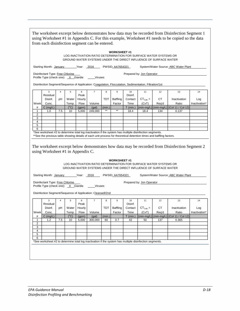
EPA Guidance Manual D-18 Disinfection Profiling and Benchmarking
The worksheet excerpt below demonstrates how data may be recorded from Disinfection Segment 1 using Worksheet #1 in Appendix C. For this example, Worksheet #1 needs to be copied so the data from each disinfection segment can be entered.
Starting Month: January Year: 2016 PWSID: AA7654321 System/Water Source: ABC Water Plant
Disinfectant Type: Free Chlorine Prepared by: Jon OperatorProfile Type (check one): X Giardia Viruses
Disinfection Segment/Sequence of Application: Coagulation, Flocculation, Sedimentation, Filtration/1st
3 4 5 6 7 8 9 10 11 12 13 14Residual Peak Disinf.Disinf. pH Water Hourly TDT Baffling Contact CTCalc = CT Inactivation Log
Week Conc. Temp. Flow Volume Factor Time (CxT) Req'd Ratio Inactivation*# C (mg/L) (oC) (gpm) (gal) (min.) T (min.) (min-mg/L) (min-mg/L) (Col 11 / Col 12)1 1.0 7.5 10 5,000 249,000 ** ** 18.4 18.4 134 0.13723456
*See worksheet #2 to determine total log inactivation if the system has multiple disinfection segments.**See the previous table showing details of each unit process for theoretical detention times and baffling factors.
WORKSHEET #1LOG INACTIVATION RATIO DETERMINATION FOR SURFACE WATER SYSTEMS OR
GROUND WATER SYSTEMS UNDER THE DIRECT INFLUENCE OF SURFACE WATER
The worksheet excerpt below demonstrates how data may be recorded from Disinfection Segment 2 using Worksheet #1 in Appendix C.
Starting Month: January Year: 2016 PWSID: AA7654321 System/Water Source: ABC Water Plant
Disinfectant Type: Free Chlorine Prepared by: Jon OperatorProfile Type (check one): X Giardia Viruses
Disinfection Segment/Sequence of Application: Clearwell/2nd
3 4 5 6 7 8 9 10 11 12 13 14Residual Peak Disinf.Disinf. pH Water Hourly TDT Baffling Contact CTCalc = CT Inactivation Log
Week Conc. Temp. Flow Volume Factor Time (CxT) Req'd Ratio Inactivation*# C (mg/L) (oC) (gpm) (gal) (min.) T (min.) (min-mg/L) (min-mg/L) (Col 11 / Col 12)1 1.2 7.5 10 5,000 300,000 60 0.7 42 50 137 0.36523456
*See worksheet #2 to determine total log inactivation if the system has multiple disinfection segments.
WORKSHEET #1LOG INACTIVATION RATIO DETERMINATION FOR SURFACE WATER SYSTEMS OR
GROUND WATER SYSTEMS UNDER THE DIRECT INFLUENCE OF SURFACE WATER

EPA Guidance Manual D-19 Disinfection Profiling and Benchmarking
The worksheet excerpt below demonstrates how data may be recorded from Disinfection Segment 3 using Worksheet #1 in Appendix C.
Starting Month: January Year: 2016 PWSID: AA7654321 System/Water Source: ABC Water Plant
Disinfectant Type: Chloramine Prepared by: Jon OperatorProfile Type (check one): X Giardia Viruses
Disinfection Segment/Sequence of Application: Transmission Pipe/3rd
3 4 5 6 7 8 9 10 11 12 13 14Residual Peak Disinf.Disinf. pH Water Hourly TDT Baffling Contact CTCalc = CT Inactivation Log
Week Conc. Temp. Flow Volume Factor Time (CxT) Req'd Ratio Inactivation*# C (mg/L) (oC) (gpm) (gal) (min.) T (min.) (min-mg/L) (min-mg/L) (Col 11 / Col 12)1 0.6 N/A 10 5,000 31,000 6.2 1.0 6.2 3.7 1,850 0.00223456
*See worksheet #2 to determine total log inactivation if the system has multiple disinfection segments.
WORKSHEET #1LOG INACTIVATION RATIO DETERMINATION FOR SURFACE WATER SYSTEMS OR
GROUND WATER SYSTEMS UNDER THE DIRECT INFLUENCE OF SURFACE WATER
The worksheet excerpt below demonstrates how to determine total Giardia log inactivation for all disinfection segments using Worksheet #2 in Appendix C.
Starting Month: January Year: 2016 PWSID: AA7654321
System/Water Source: ABC Water Plant Prepared by: Jon Operator
Disinfectant Type: Chlorine/ChloramineProfile Type (check one): X Giardia Viruses
SumDisinfection Disinfection Disinfection Disinfection Disinfection of Total
Week Segment Segment Segment Segment Segment Inactivation Log# 1 2 3 4 5 Ratios Inactivation1
1 0.137 0.365 0.002 0.504 1.5123456
1Giardia : Log Inactivation = 3 x Sum of Inactivation Ratios Viruses: Log Inactivation = 4 x Sum of Inactivation Ratios (or a method approved by the State)
Inactivation Ratio for each disinfection segment from Worksheet #1
TOTAL LOG INACTIVATION DETERMINATION FOR SURFACE WATER SYSTEMS ORGROUND WATER SYSTEMS UNDER THE DIRECT INFLUENCE OF SURFACE WATER
WORKSHEET #2

EPA Guidance Manual D-20 Disinfection Profiling and Benchmarking
Example D-3. Develop a Disinfection Profile and Benchmark for a PWS with Multiple Disinfection Segments
In this example, a conventional filtration treatment plant adds ozone in contact chambers at the head of the plant and injects chlorine after the clearwell for primary disinfection in the transmission pipe leaving the treatment plant (before the first customer). The ozone residual is measured at each ozone contact chamber and the chlorine residual is measured in the transmission pipe. Because ozone does not maintain a residual for any extended period of time, there is no disinfection segment for the coagulation, flocculation, sedimentation, filtration, and clearwell portions of the plant.
In the Long Term 2 Enhanced Surface Water Treatment Rule Toolbox Guidance Manual, April 2010, the EPA provides four methods for calculating CT in an ozone contactor: the T10 method, the Continuous Stirred Reactor Method (CSTR), the extended T10 method, and the extended CSTR method. Selecting the appropriate method(s) to use depends on the configuration of the ozone contactor, the availability of state-approved tracer testing results, and the amount of process evaluation and monitoring that a PWS wishes to undertake. Example D-3 demonstrates the T10 method. The T10 method is determined using tracer studies (see Appendix E) and is the time at which 90 percent of the water that enters the chamber will remain for at least T10 minutes. If no tracer study data are available for determining T10, the EPA recommends using the CSTR method. The CSTR method uses the hydraulic detention time of the ozone contactor for estimating contact time. Examples for all four methods can be found in the Long Term 2 Enhanced Surface Water Treatment Rule Toolbox Guidance Manual, April 2010.
Sedimentation
FlocculationCoagulation Filtration
Clearwell
ToDistribution
System
Disinfection Segment 4Monitoring Point
Chlorine Residual = 0.8 mg/LTemperature = 0.5 oC
pH = 7.0
DisinfectionSegm
ent 4
Ozone Contact Chambers
DisinfectionSegment 1
DisinfectionSegment 2
DisinfectionSegment 3
ChlorineSee enlarged drawing below
C1out = 0.5 mg/L
C2in = 0.4 mg/L
C2out = 0.6 mg/L C3in = 0.6 mg/L
C3out = 0.1 mg/LC1in = 0.0 mg/L
Chamber 1 Chamber 3Chamber 2
Temp = 0.5 oC Temp = 0.5 oC
Temp = 0.5 oC Temp = 0.5 oC
DisinfectionSegment 1
DisinfectionSegment 2
DisinfectionSegment 3
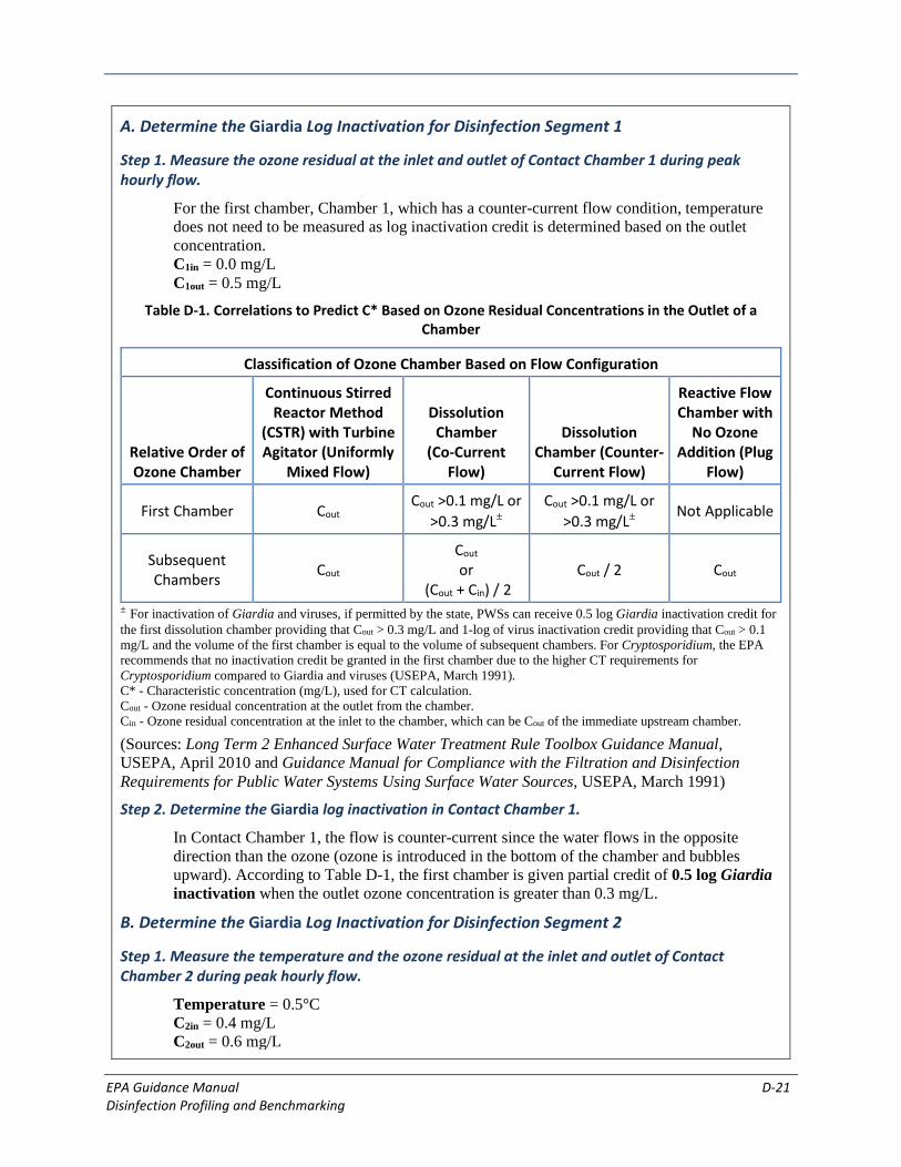
EPA Guidance Manual D-21 Disinfection Profiling and Benchmarking
A. Determine the Giardia Log Inactivation for Disinfection Segment 1
Step 1. Measure the ozone residual at the inlet and outlet of Contact Chamber 1 during peak hourly flow.
For the first chamber, Chamber 1, which has a counter-current flow condition, temperature does not need to be measured as log inactivation credit is determined based on the outlet concentration. C1in = 0.0 mg/L C1out = 0.5 mg/L
Table D-1. Correlations to Predict C* Based on Ozone Residual Concentrations in the Outlet of a Chamber
Classification of Ozone Chamber Based on Flow Configuration
Relative Order of Ozone Chamber
Continuous Stirred Reactor Method
(CSTR) with Turbine Agitator (Uniformly
Mixed Flow)
Dissolution Chamber
(Co-Current Flow)
Dissolution Chamber (Counter-
Current Flow)
Reactive Flow Chamber with
No Ozone Addition (Plug
Flow)
First Chamber Cout Cout >0.1 mg/L or
>0.3 mg/L± Cout >0.1 mg/L or
>0.3 mg/L± Not Applicable
Subsequent Chambers Cout
Cout or
(Cout + Cin) / 2 Cout / 2 Cout
± For inactivation of Giardia and viruses, if permitted by the state, PWSs can receive 0.5 log Giardia inactivation credit for the first dissolution chamber providing that Cout > 0.3 mg/L and 1-log of virus inactivation credit providing that Cout > 0.1 mg/L and the volume of the first chamber is equal to the volume of subsequent chambers. For Cryptosporidium, the EPA recommends that no inactivation credit be granted in the first chamber due to the higher CT requirements for Cryptosporidium compared to Giardia and viruses (USEPA, March 1991). C* - Characteristic concentration (mg/L), used for CT calculation. Cout - Ozone residual concentration at the outlet from the chamber. Cin - Ozone residual concentration at the inlet to the chamber, which can be Cout of the immediate upstream chamber.
(Sources: Long Term 2 Enhanced Surface Water Treatment Rule Toolbox Guidance Manual, USEPA, April 2010 and Guidance Manual for Compliance with the Filtration and Disinfection Requirements for Public Water Systems Using Surface Water Sources, USEPA, March 1991)
Step 2. Determine the Giardia log inactivation in Contact Chamber 1.
In Contact Chamber 1, the flow is counter-current since the water flows in the opposite direction than the ozone (ozone is introduced in the bottom of the chamber and bubbles upward). According to Table D-1, the first chamber is given partial credit of 0.5 log Giardia inactivation when the outlet ozone concentration is greater than 0.3 mg/L.
B. Determine the Giardia Log Inactivation for Disinfection Segment 2
Step 1. Measure the temperature and the ozone residual at the inlet and outlet of Contact Chamber 2 during peak hourly flow.
Temperature = 0.5°C C2in = 0.4 mg/L C2out = 0.6 mg/L

EPA Guidance Manual D-22 Disinfection Profiling and Benchmarking
Step 2. Determine C in Contact Chamber 2.
Table D-1. Correlations to Predict C* Based on Ozone Residual Concentrations in the Outlet of a Chamber
Classification of Ozone Chamber Based on Flow Configuration
Relative Order of Ozone Chamber
Continuous Stirred Reactor Method
(CSTR) with Turbine Agitator (Uniformly
Mixed Flow)
Dissolution Chamber
(Co-Current Flow)
Dissolution Chamber (Counter-
Current Flow)
Reactive Flow Chamber with
No Ozone Addition (Plug
Flow)
First Chamber Cout Cout >0.1 mg/L or
>0.3 mg/L± Cout >0.1 mg/L or
>0.3 mg/L± Not Applicable
Subsequent Chambers Cout
Cout or
(Cout + Cin) / 2 Cout / 2 Cout
± For inactivation of Giardia and viruses, if permitted by the state, PWSs can receive 0.5 log Giardia inactivation credit for the first dissolution chamber providing that Cout > 0.3 mg/L and 1-log of virus inactivation credit providing that Cout > 0.1 mg/L and the volume of the first chamber is equal to the volume of subsequent chambers. For Cryptosporidium, the EPA recommends that no inactivation credit be granted in the first chamber due to the higher CT requirements for Cryptosporidium compared to Giardia and viruses (USEPA, March 1991). C* - Characteristic concentration (mg/L), used for CT calculation. Cout - Ozone residual concentration at the outlet from the chamber. Cin - Ozone residual concentration at the inlet to the chamber, which can be Cout of the immediate upstream chamber.
(Sources: Long Term 2 Enhanced Surface Water Treatment Rule Toolbox Guidance Manual, USEPA, April 2010 and Guidance Manual for Compliance with the Filtration and Disinfection Requirements for Public Water Systems Using Surface Water Sources, USEPA, March 1991)
As in Contact Chamber 1, in Contact Chamber 2 the flow is counter-current since the water flows in the opposite direction that the ozone flows. According to Table D-1, C = Cout / 2 for subsequent contact chambers with counter-current flow.
C = C2out / 2 C = 0.6 mg/L / 2 C = 0.3 mg/L
Step 3. Determine the contact time in Contact Chamber 2.
The contact time for all of the ozone contact chambers taken together was determined by a tracer study to be 15 minutes at peak hourly flow. The total contact time can be divided proportionally by volume between all three chambers if the chambers with final concentrations of zero (non-detectable) do not make up 50% or greater of the total volume of the chambers. Since the final concentration in all chambers is greater than zero and since the contact chambers all have equal volumes, the contact time can be divided equally between all three chambers:
T = Ttot / 3 chambers = 15 min / 3 chambers = 5 minutes per chamber

EPA Guidance Manual D-23 Disinfection Profiling and Benchmarking
Step 4. Calculate CTcalc in Contact Chamber 2.
CTcalc = C x T CTcalc = 0.3 mg/L x 5 min CTcalc = 1.5 min-mg/L
Step 5. Locate appropriate CT table.
The table for 3-log inactivation of Giardia by ozone is Table B-5 in Appendix B.
Step 6. Identify the appropriate portion of the table based on operating conditions.
Locate the column for 0.5°C (< = 1°C).
Table B-5
CT Values for 3-Log Inactivation of Giardia Cysts by Ozone
Temperature (°C)
< = 1 5 10 15 20 25
2.9 1.90 1.43 0.95 0.72 0.48
Step 7. Obtain CT99.9 value.
From this chart it is determined that the value of CT for 3-log inactivation by ozone at 0.5°C is 2.9 min-mg/L.
CT99.9 = 2.9 min-mg/L
Step 8. Calculate the Giardia inactivation ratio for Disinfection Segment 2.
Inactivation ratio = CTcalc / CT99.9 Inactivation ratio = (1.5 min-mg/L / 2.9 min-mg/L) Inactivation ratio = 0.517
Step 9. Calculate Giardia inactivation for Disinfection Segment 2.
Giardia log inactivation = 3 x (CTcalc / CT99.9) Giardia log inactivation = 3 x 0.517 Giardia log inactivation = 1.55
C. Determine the Giardia Log Inactivation for Disinfection Segment 3

EPA Guidance Manual D-24 Disinfection Profiling and Benchmarking
Step 1. Measure the temperature and the ozone residual at the inlet and outlet of Contact Chamber 3 during peak hourly flow.
Temperature = 0.5°C C3in = 0.6 mg/L C3out = 0.1 mg/L
Step 2. Determine C in Contact Chamber 3.
Table D-1. Correlations to Predict C* Based on Ozone Residual Concentrations in the Outlet of a Chamber
Classification of Ozone Chamber Based on Flow Configuration
Relative Order of Ozone Chamber
Continuous Stirred Reactor Method
(CSTR) with Turbine Agitator (Uniformly
Mixed Flow)
Dissolution Chamber
(Co-Current Flow)
Dissolution Chamber (Counter-
Current Flow)
Reactive Flow Chamber with
No Ozone Addition (Plug
Flow)
First Chamber Cout Cout >0.1 mg/L or
>0.3 mg/L± Cout >0.1 mg/L or
>0.3 mg/L± Not Applicable
Subsequent Chambers Cout
Cout or
(Cout + Cin) / 2 Cout / 2 Cout
± For inactivation of Giardia and viruses, if permitted by the state, PWSs can receive 0.5 log Giardia inactivation credit for the first dissolution chamber providing that Cout > 0.3 mg/L and 1-log of virus inactivation credit providing that Cout > 0.1 mg/L and the volume of the first chamber is equal to the volume of subsequent chambers. For Cryptosporidium, the EPA recommends that no inactivation credit be granted in the first chamber due to the higher CT requirements for Cryptosporidium compared to Giardia and viruses (USEPA, March 1991). C* - Characteristic concentration (mg/L), used for CT calculation. Cout - Ozone residual concentration at the outlet from the chamber. Cin - Ozone residual concentration at the inlet to the chamber, which can be Cout of the immediate upstream chamber.
(Sources: Long Term 2 Enhanced Surface Water Treatment Rule Toolbox Guidance Manual, USEPA, April 2010 and Guidance Manual for Compliance with the Filtration and Disinfection Requirements for Public Water Systems Using Surface Water Sources, USEPA, March 1991)
In Contact Chamber 3, the flow is co-current since the water flows in the same direction that the ozone flows (see directional arrows in the diagram above). According to Table D-1, C = (Cout + Cin) / 2 for contact chambers with co-current flow.
C = (C3in + C3out) / 2 C = (0.6 mg/L + 0.1 mg/L) / 2 C = 0.35 mg/L
Step 3. Determine the contact time in Contact Chamber 3.
It was determined in Part B, Step 3 of this example that the contact time in each chamber is 5 minutes.
T = 5 minutes

EPA Guidance Manual D-25 Disinfection Profiling and Benchmarking
Step 4. Calculate CTcalc in Contact Chamber 3.
CTcalc = C x T CTcalc = 0.35 mg/L x 5 min CTcalc = 1.75 min-mg/L
Step 5. Locate appropriate CT table.
The table for 3-log inactivation of Giardia by ozone is Table B-5 in Appendix B.
Step 6. Identify the appropriate portion of the table based on operating conditions.
Locate the column for 0.5°C (< = 1°C).
Table B-5
CT Values for 3-Log Inactivation of Giardia Cysts by Ozone
Temperature (ºC)
< = 1 5 10 15 20 25
2.9 1.90 1.43 0.95 0.72 0.48
Step 7. Obtain CT99.9 value.
From this chart it is determined that the value of CT for 3-log inactivation by ozone at 0.5°C is 2.9 min-mg/L.
CT99.9 = 2.9 min-mg/L
Step 8. Calculate the Giardia inactivation ratio for Disinfection Segment 3.
Inactivation ratio = CTcalc / CT99.9 Inactivation ratio = (1.75 min-mg/L / 2.9 min-mg/L) Inactivation ratio = 0.603
Step 9. Calculate Giardia inactivation for Disinfection Segment 3.
Giardia log inactivation = 3 x (CTcalc / CT99.9) Giardia log inactivation = 3 x 0.603 Giardia log inactivation = 1.81

EPA Guidance Manual D-26 Disinfection Profiling and Benchmarking
D. Determine Giardia Log Inactivation for Disinfection Segment 4
Step 1. Determine the peak hourly flow.
From the raw water pump records the peak hourly flow (Q) is determined to be 5,000 gpm.
Step 2. Measure chlorine residual, temperature, and pH during peak hourly flow at the chlorine monitoring point located prior to the first customer in the distribution system.
Temperature = 0.5°C pH = 7.0 Chlorine residual = Cchlorine = 0.8 mg/L
Step 3. Measure the physical dimensions of the pipe.
5,280 Feet
Side View
End View(Closeup)
Diameter = 12 in
Measure the length of the pipe from the chlorine addition point to the chlorine monitoring point located prior to the first customer in the distribution system. Measure the inner pipe diameter to obtain the volume of water in the pipe rather than the volume of the pipe itself.
Diameter = 12 in x (1 ft / 12 in) = 1.0 ft Length = 5,280 ft
Step 4. Calculate the volume of the water in the pipe.
Volume (V) = π x Radius2 x Length π = 3.14 (constant)
Radius = Diameter / 2 = 1.0 / 2 = 0.5 ft V = 3.14 x (0.5 ft)2 x 5,280 ft = 4,140 ft3 V= 4,140 ft3 x (7.48 gal / ft3) V = 31,000 gallons

EPA Guidance Manual D-27 Disinfection Profiling and Benchmarking
Step 5. Calculate the Theoretical Detention Time in the pipe.
Theoretical Detention Time (TDT) = V / Q TDT = 31,000 gal / 5,000 gpm TDT = 6.2 minutes
Step 6. Determine the baffling factor for the pipe.
Baffling Factor (BF) = 1.0 (from Table G-1 in Appendix G for a pipe)
Step 7. Calculate the contact time of the disinfectant in the pipe.
Contact Time (T) = TDT x BF T = 6.2 min x 1.0 T = 6.2 minutes
Step 8. Calculate the CT for the disinfection segment.
CTcalc = Cchlorine x T CTcalc = 0.8 mg/L x 6.2 min CTcalc = 5.0 min-mg/L
Step 9. Determine the required CT99.9 necessary to obtain 3-log Giardia inactivation.
The required CT value for 3-log Giardia inactivation (CT99.9) is obtained by using CT Table B-1 in Appendix B, CT Values for 3-Log Inactivation of Giardia Cysts by Free Chlorine. The CT99.9 is 205 min-mg/L for a pH of 7.0, temperature of 0.5°C, and Cchlorine of 0.8 mg/L. The relevant section of Table B-1 is reprinted below and the pertinent section of the table is highlighted.
Excerpt from Table B-1
CT Values for 3-Log Inactivation of Giardia Cysts by Free Chlorine (0.5°C portion of table, for concentrations from 0.4 to 1.2 mg/L)
Chlorine Concentration
(mg/L)
Temperature = 0.5°C
pH
<=6.0 6.5 7.0 7.5 8.0 8.5 9.0
<=0.4 137 163 195 237 277 329 390
0.6 141 169 200 239 286 342 407
0.8 145 172 205 246 295 354 422
1.0 148 176 210 253 304 365 437
1.2 152 180 215 259 313 376 451

EPA Guidance Manual D-28 Disinfection Profiling and Benchmarking
Step 10. Calculate the Giardia inactivation ratio for the pipe.
Inactivation ratio = CTcalc / CT99.9 Inactivation ratio = (5.0 min-mg/L / 205 min-mg/L) Inactivation ratio = 0.024
Step 11. Calculate the Giardia log inactivation for the pipe.
Log inactivation = 3 x CTcalc / CT99.9 Log inactivation = 3 x 0.024 Log inactivation = 0.07
The log inactivation of Giardia for Disinfection Segment 4 is 0.07.
E. Calculate the Total Giardia Inactivation for All Disinfection Segments
Step 1. Sum the Giardia log inactivation credits for all of the disinfection segments to determine the total Giardia log inactivation achieved.
From Disinfection Segment 1: Giardia log inactivation = 0.50
From Disinfection Segment 2: Giardia log inactivation = 1.55
From Disinfection Segment 3: Giardia log inactivation = 1.81
From Disinfection Segment 4: Giardia log inactivation = 0.07
Total Giardia log inactivation = 0.50 + 1.55 + 1.81 + 0.07 = 3.93
Assuming the PWS received a 2.5 log Giardia removal credit from the state for conventional filtration, it must achieve at least 0.5 log Giardia inactivation for a total 3.0 log Giardia removal and/or inactivation as required in the Surface Water Treatment Rule (40 CFR Section 141.70(a)(1)). The value of 3.93 log Giardia inactivation exceeds the required 0.5 log Giardia inactivation.

EPA Guidance Manual D-29 Disinfection Profiling and Benchmarking
F. Determine Virus Log Inactivation for Disinfection Segment 1 Step 1. Determine the virus log inactivation in Contact Chamber 1.
Table D-1. Correlations to Predict C* Based on Ozone Residual Concentrations in the Outlet of a Chamber
Classification of Ozone Chamber Based on Flow Configuration
Relative Order of Ozone Chamber
Continuous Stirred Reactor Method
(CSTR) with Turbine Agitator (Uniformly
Mixed Flow)
Dissolution Chamber
(Co-Current Flow)
Dissolution Chamber (Counter-
Current Flow)
Reactive Flow Chamber with
No Ozone Addition (Plug
Flow)
First Chamber Cout Cout >0.1 mg/L or
>0.3 mg/L± Cout >0.1 mg/L or
>0.3 mg/L± Not Applicable
Subsequent Chambers Cout
Cout or
(Cout + Cin) / 2 Cout / 2 Cout
± For inactivation of Giardia and viruses, if permitted by the state, PWSs can receive 0.5 log Giardia inactivation credit for the first dissolution chamber providing that Cout > 0.3 mg/L and 1-log of virus inactivation credit providing that Cout > 0.1 mg/L and the volume of the first chamber is equal to the volume of subsequent chambers. For Cryptosporidium, the EPA recommends that no inactivation credit be granted in the first chamber due to the higher CT requirements for Cryptosporidium compared to Giardia and viruses (USEPA, March 1991). C* - Characteristic concentration (mg/L), used for CT calculation. Cout - Ozone residual concentration at the outlet from the chamber. Cin - Ozone residual concentration at the inlet to the chamber, which can be Cout of the immediate upstream chamber.
(Sources: Long Term 2 Enhanced Surface Water Treatment Rule Toolbox Guidance Manual, USEPA, April 2010 and Guidance Manual for Compliance with the Filtration and Disinfection Requirements for Public Water Systems Using Surface Water Sources, USEPA, March 1991)
In Contact Chamber 1, the flow is counter-current since the water flows in the opposite direction than the ozone (ozone is introduced in the bottom of the chamber and bubbles upward). According to Table D-1, the first chamber is given partial credit of 1 virus log inactivation when the outlet ozone concentration is greater than 0.1 mg/L.
G. Determine Virus Log Inactivation for Disinfection Segment 2 Step 1. Determine the required CT99.99 necessary to obtain 4-log virus inactivation for Contact Chamber 2.
The required CT value for 4-log virus inactivation (CT99.99) is obtained by using CT Table B-6 in Appendix B, CT Values for 4-Log Inactivation of Viruses by Ozone. In this example the required CT99.99 is 1.8 min-mg/L for a temperature of 0.5°C.
Table B-6
CT Values for 4-Log Inactivation of Viruses by Ozone
Temperature (°C)
< = 1 5 10 15 20 25
1.8 1.2 1.0 0.6 0.5 0.3
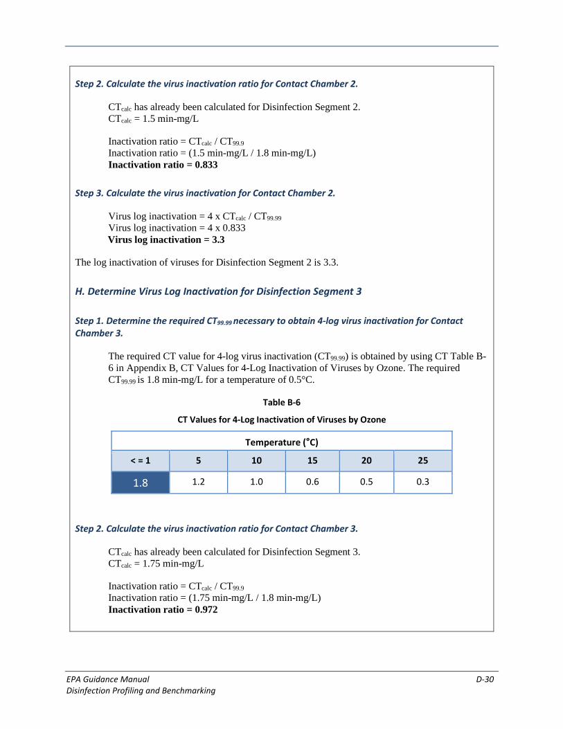
EPA Guidance Manual D-30 Disinfection Profiling and Benchmarking
Step 2. Calculate the virus inactivation ratio for Contact Chamber 2.
CTcalc has already been calculated for Disinfection Segment 2. CTcalc = 1.5 min-mg/L
Inactivation ratio = CTcalc / CT99.9 Inactivation ratio = (1.5 min-mg/L / 1.8 min-mg/L) Inactivation ratio = 0.833
Step 3. Calculate the virus inactivation for Contact Chamber 2.
Virus log inactivation = 4 x CTcalc / CT99.99 Virus log inactivation = 4 x 0.833 Virus log inactivation = 3.3
The log inactivation of viruses for Disinfection Segment 2 is 3.3.
H. Determine Virus Log Inactivation for Disinfection Segment 3
Step 1. Determine the required CT99.99 necessary to obtain 4-log virus inactivation for Contact Chamber 3.
The required CT value for 4-log virus inactivation (CT99.99) is obtained by using CT Table B-6 in Appendix B, CT Values for 4-Log Inactivation of Viruses by Ozone. The required CT99.99 is 1.8 min-mg/L for a temperature of 0.5°C.
Table B-6
CT Values for 4-Log Inactivation of Viruses by Ozone
Temperature (°C)
< = 1 5 10 15 20 25
1.8 1.2 1.0 0.6 0.5 0.3
Step 2. Calculate the virus inactivation ratio for Contact Chamber 3.
CTcalc has already been calculated for Disinfection Segment 3. CTcalc = 1.75 min-mg/L
Inactivation ratio = CTcalc / CT99.9 Inactivation ratio = (1.75 min-mg/L / 1.8 min-mg/L) Inactivation ratio = 0.972
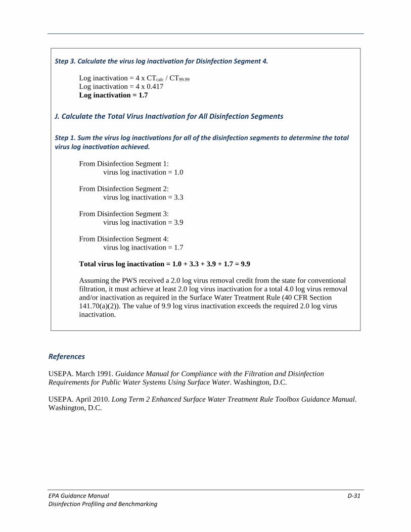
EPA Guidance Manual D-31 Disinfection Profiling and Benchmarking
Step 3. Calculate the virus log inactivation for Disinfection Segment 4.
Log inactivation = 4 x CTcalc / CT99.99 Log inactivation = 4 x 0.417 Log inactivation = 1.7
J. Calculate the Total Virus Inactivation for All Disinfection Segments
Step 1. Sum the virus log inactivations for all of the disinfection segments to determine the total virus log inactivation achieved.
From Disinfection Segment 1: virus log inactivation = 1.0
From Disinfection Segment 2: virus log inactivation = 3.3
From Disinfection Segment 3: virus log inactivation = 3.9
From Disinfection Segment 4: virus log inactivation = 1.7
Total virus log inactivation = 1.0 + 3.3 + 3.9 + 1.7 = 9.9
Assuming the PWS received a 2.0 log virus removal credit from the state for conventional filtration, it must achieve at least 2.0 log virus inactivation for a total 4.0 log virus removal and/or inactivation as required in the Surface Water Treatment Rule (40 CFR Section 141.70(a)(2)). The value of 9.9 log virus inactivation exceeds the required 2.0 log virus inactivation.
References
USEPA. March 1991. Guidance Manual for Compliance with the Filtration and Disinfection Requirements for Public Water Systems Using Surface Water. Washington, D.C. USEPA. April 2010. Long Term 2 Enhanced Surface Water Treatment Rule Toolbox Guidance Manual. Washington, D.C.

EPA Guidance Manual D-32 Disinfection Profiling and Benchmarking
This Page Intentionally Left Blank

EPA Guidance Manual E-1 Disinfection Profiling and Benchmarking
Appendix E — Tracer Studies
E.1 Introduction
Information in this appendix is based on Appendix C in the Guidance Manual for Compliance with the Filtration and Disinfection Requirements for Public Water Systems Using Surface Water Sources (USEPA, 1991). For more information on tracer studies, readers are encouraged to consult Appendix C in the Guidance Manual for Compliance with the Filtration and Disinfection Requirements for Public Water Systems Using Surface Water Sources (USEPA, 1991) or Tracer Studies in Water Treatment Facilities: A Protocol and Case Studies (Teefy, 1996).
As indicated in Chapter 4, fluid passing through a pipe is assumed to have a detention time equal to the theoretical or mean residence time at a particular flow rate. However, in mixing basins, storage reservoirs, and other treatment plant process units, utilities may be required to determine the contact time for the calculation of CT through tracer studies or other methods approved by the state.
The contact time of mixing basins and storage reservoirs used in calculating CT should be the minimum detention time experienced by 90 percent of the water passing through the unit. This detention time was designated as T10 according to the convention adopted by Thirumurthi (1969). A profile of the flow through the basin over time can be generated by tracer studies. Information provided by these studies may be used for estimating the detention time, T10, for the purpose of calculating CT. (Note: T10 is referred to as “T” elsewhere in this document. However, for consistency with the Guidance Manual for Compliance with the Filtration and Disinfection Requirements for Public Water Systems Using Surface Water Sources (USEPA, 1991), T10 is used in this appendix.)
This appendix presents a brief synopsis of tracer study methods, procedures, and data evaluation. More detailed information about conducting tracer studies is available in Appendix C of the Guidance Manual for Compliance with the Filtration and Disinfection Requirements for Public Water Systems Using Surface Water Sources (USEPA, 1991). It is important to obtain assistance from the state before conducting a tracer study to ensure state approval of the results.
E.2 Flow Evaluation
Although detention time is proportional to flow, it is not generally a linear function. Tracer studies may establish detention times for the range of flow rates experienced within each disinfectant segment. PWSs should note that a single flow rate might not characterize the flow through the entire PWS. With a series of reservoirs, clearwells, and storage tanks, flow will vary between each portion of the PWS.
Ideally, tracer tests should be performed for at least four flow rates that span the entire range of flow for the segment being tested. The flow rates should be separated by approximately equal intervals to span the range of operation, with one near average flow, two greater than average, and one less than average flow. The flows should also be selected so that the highest test flow rate is at least 91 percent of the highest flow rate expected to ever occur in that segment. Four data points should assure a good definition of the segment’s hydraulic profile.

EPA Guidance Manual E-2 Disinfection Profiling and Benchmarking
The results of the tracer tests performed for different flow rates should be used to generate plots of T10 versus flow (Q) for each segment. A smooth line is drawn through the points on each graph to create a curve from which T10 may be read for the corresponding flow at peak hourly flow conditions. Refer to Appendix C, section C.1.7 of the Guidance Manual for Compliance with the Filtration and Disinfection Requirements for Public Water Systems Using Surface Water Sources (USEPA, 1991), for an illustration of this procedure.
The most accurate tracer test results are obtained when flow is constant through the segment during the course of the test. Therefore, the tracer study should be conducted at a constant flow whenever practical. For a treatment plant consisting of two or more equivalent process trains, a constant flow tracer test can be performed on a segment of the plant by holding the flow through one of the trains constant while operating the parallel train(s) to absorb any flow variations. Flow variations during tracer tests in treatment systems without parallel trains or with single clearwells and storage reservoirs are more difficult to avoid. In these instances, T10 should be recorded at the average flow rate over the course of the test.
E.3 Volume Evaluation
In addition to flow conditions, detention times determined by tracer studies depend on the water level and subsequent volume in treatment units. This is particularly pertinent to storage tanks, reservoirs, and clearwells, which, in addition to being contact basins for disinfection are also often used as equalization storage for distribution system demands and storage for backwashing. For these treatment units, the water levels in the reservoirs vary to meet the PWS demands. The actual detention time of these contact basins will also vary depending on whether they are emptying or filling.
For some process units, especially sedimentation basins that are operated at a near constant level (that is, flow in equals flow out), the detention time determined by tracer tests should be sufficient for calculating CT when the basin is operating at water levels greater than or equal to the level at which the test was performed. When conducting a tracer study to determine the detention time, a water level at or slightly below, but not above, the normal minimum operating level is recommended. For many plants, the water level in a clearwell or storage tank varies between high and low levels in response to distribution system demands. In such instances, in order to obtain a conservative estimate of the contact time, the tracer study should be conducted during a period when the tank level is falling (flow out greater than flow in).
E.4 Disinfection Segments
For PWSs that apply disinfectant(s) at more than one point or choose to profile the residual from one point of application, tracer studies should be conducted to determine T10 for each segment containing process unit(s). The T10 for a segment is used along with the residual disinfectant concentration prior to the next disinfectant application or monitoring point to determine the CTcalc for that segment. The inactivation ratio for the section is then determined. The total log inactivation achieved with all disinfection segments can then be determined by summing the inactivation ratios for all sections as explained in Chapter 5 of this document.
For PWSs that have two or more units of identical size and configuration, tracer studies could be conducted on one of the units but applied to both. The resulting graph of T10 versus flow can be used to determine T10 for all identical units.

EPA Guidance Manual E-3 Disinfection Profiling and Benchmarking
PWSs with more than one segment in the treatment plant that are conducting a tracer study may determine T10 for each segment:
• By individual tracer studies through each segment. • By one tracer study across the treatment system.
If possible, tracer studies should be conducted on each segment to determine the T10 for each segment. In order to minimize the time needed to conduct studies on each segment, the tracer studies should be started at the last segment of the treatment train prior to the first customer and completed with the first segment. Conducting the tracer studies in this order will prevent the interference of residual tracer material with subsequent studies.
For ozone contactors, flocculators, or any basin containing mixing, tracer studies should be conducted for the range of mixing used in the process. In ozone contactors, air or oxygen should be added in lieu of ozone to prevent degradation of the tracer. The flow rate of air or oxygen used for the contactor should be applied during the study to simulate actual operation. Tracer studies should then be conducted at several air/oxygen to water ratios to provide data for the complete range of ratios used at the plant. For flocculators, tracer studies should be conducted for various mixing intensities to provide data for the complete range of operations.
E.5 Tracer Study Methods
This section discusses the two most common methods of tracer addition employed in water treatment evaluations, the step-dose method, and the slug-dose method. Tracer study methods involve the application of chemical dosages and tracking the resulting effluent concentration as a function of time. The effluent concentration profile is evaluated to determine the detention time, T10.
In preparation for beginning a tracer study, the raw water background concentration of the chosen tracer chemical should be established. The background concentration is important, not only to aid in the selection of the tracer dosage, but also to facilitate proper evaluation of the data.
The background tracer concentration should be determined by monitoring for the tracer chemical prior to beginning the test. The sampling point(s) for the pre-tracer study monitoring should be the same as the points to be used for residual monitoring to determine CT values. PWSs should use the following monitoring procedure:
• Prior to the start of the test, regardless of whether the chosen tracer material is a treatment chemical, the tracer concentration in the water is monitored at the sampling point where the disinfectant residual will be measured for CT calculations.
• If a background tracer concentration is detected, monitor it until a constant concentration, at or below the raw water background level, is achieved. This measured concentration is the baseline tracer concentration.
Following the determination of the tracer dosage, feed and monitoring point(s), and a baseline tracer concentration, tracer testing can begin.
Equal sampling intervals, as could be obtained from automatic sampling, are not required for either tracer study method. However, using equal sample intervals for the slug-dose method can simplify the analysis

EPA Guidance Manual E-4 Disinfection Profiling and Benchmarking
of the data. During testing, the time and tracer residual of each measurement should also be recorded on a data sheet. In addition, the water level, flow, and temperature should be recorded during the test.
E.5.1 Step-Dose Method
The step-dose method entails introduction of a tracer chemical at a constant dosage until the concentration at the desired end point reaches a steady-state level. At time zero, the tracer chemical feed is started and left at a constant rate for the duration of the test. Over the course of the test, the tracer residual should be monitored at the required sampling point(s) at a frequency determined by the overall detention time and site-specific considerations. As a general guideline, sampling at intervals of 2 to 5 minutes should provide data for a well-defined plot of tracer concentration versus time. If on-site analysis is available, less frequent residual monitoring may be possible until a change in residual concentration is first detected. Regular sampling is continued until the residual concentration reaches a steady-state value.
One graphical method of evaluating step-dose test data involves plotting a graph of dimensionless concentration (tracer concentration (C) / applied tracer concentration (Co)) versus time and reading the value for T10 directly from the graph at the appropriate dimensionless concentration. Alternatively, the data from step-dose tracer studies may be evaluated numerically by developing a semi-logarithmic plot of the dimensionless data. The semi-logarithmic plot allows a straight line to be drawn through the data. The resulting equation of the line is used to calculate the T10 value, assuming that the correlation coefficient indicates a good statistical fit (0.9 or above). Drawing a smooth curve through the data discredits scattered data points from step-dose tracer tests.
Step-dose tracer studies are frequently employed in drinking water applications for the following reasons:
• The resulting normalized concentration versus time profile is directly used to determine T10, the detention time required for calculating CT; and,
• Very often, the necessary feed equipment is available to provide a constant rate of application of the tracer chemical.
One other advantage of the step-dose method is that the data may be verified by comparing the concentration versus elapsed time profile for samples collected at the start of dosing with the profile obtained when the tracer feed is discontinued.
E.5.2 Slug-Dose Method
In the slug-dose method, a large instantaneous dose of tracer is added to the incoming water and samples are taken at the exit of the unit over time as the tracer passes through the unit. At time zero for the slug-dose method, the dose of tracer is added to the influent of the unit. The same sampling locations and frequencies described for step-dose method tests also apply to slug-dose method tracer studies. One exception for this method is that the tracer concentration profile will not equilibrate to a steady-state concentration. Because of this, the tracer should be monitored frequently enough to ensure acquisition of data needed to identify the peak tracer concentration.
Slug-dose method tests should be checked by performing a material balance to ensure that all tracer that was fed is recovered. In other words, mass applied equals mass discharged.

EPA Guidance Manual E-5 Disinfection Profiling and Benchmarking
Data from slug-dose tracer tests may be analyzed by converting it to the mathematically equivalent of step-dose data and using the techniques discussed above for the step-dose method to determine T10. A graph of dimensionless concentration versus time should be drawn which represents the results of a slug-dose tracer test. The key to converting between the data forms is obtaining the total area under the slug-dose data curve. This area is found by integrating the curve graphically or numerically. The conversion to step-dose data is then completed in several mathematical steps involving the total area.
Slug-dose concentration profiles can have many shapes, depending on the hydraulics of the basin. Therefore, slug-dose data points should not be discredited by drawing a smooth curve through the data prior to its conversion to step-dose data.
A disadvantage of the slug-dose method is that very concentrated solutions are needed for the dose in order to adequately define the concentration versus time profile. Intensive mixing is therefore necessary to minimize potential density-current effects and to obtain a uniform distribution of the instantaneous tracer dose across the basin. This is inherently difficult under water flow conditions often existing at inlets to basins. Other disadvantages of using the slug-dose method include:
• The concentration and volume of the instantaneous tracer dose needs to be carefully computed to provide an adequate tracer profile at the effluent of the basin;
• The resulting concentration versus time profile should not be used to directly determine T10 without further manipulation; and,
• A mass balance on the treatment segment should be used to determine whether the tracer was completely recovered.
One advantage of this method is that it may be applied where chemical feed equipment is not available at the desired point of addition, or where the equipment available does not have the capacity to provide the necessary concentration of the chosen tracer chemical. Although, in general, the step-dose procedure offers the greatest simplicity, both methods are theoretically equivalent for determining T10. Either method or another method may be used for conducting drinking water tracer studies, and the choice of method may be determined by site-specific constraints or the PWS’s experience.
E.6 Tracer Selection
An important step in any tracer study is the selection of a chemical to be used as the tracer. Ideally, the selected tracer chemical should be readily available, conservative (that is, not consumed or removed during treatment), easily monitored, and acceptable for use in potable water supplies. Chloride and fluoride are nontoxic and approved for potable water use and are typically the most common tracer chemicals employed in drinking water plants. Rhodamine WT can be used as a fluorescent tracer in water flow studies in accordance with the following guidelines:
• Raw water concentrations should be limited to a maximum concentration of 10 mg/L;
• Drinking water concentrations should not exceed 0.1 µg/L;
• Studies that result in human exposure to the dye should be brief and infrequent; and,
• Concentrations as low as 2 µg/L can be used in tracer studies because of the low detection level in the range of 0.1 to 0.2 µg/L.

EPA Guidance Manual E-6 Disinfection Profiling and Benchmarking
The use of Rhodamine B as a tracer in water flow studies is not recommended by the EPA.
The choice of a tracer chemical can be made based, in part, on the selected dosing method and on the availability of chemical feeding equipment. For example, the high density of concentrated salt solutions and their potential for inducing density currents usually precludes chloride and fluoride as the selected chemical for slug-dose tracer tests.
Fluoride can be a convenient tracer chemical for step-dose tracer tests of clearwells because it is frequently applied for finished water treatment. However, when fluoride is used in tracer tests on clarifiers, allowances should be made for fluoride that is absorbed on floc and settles out of water (Hudson, 1975). Additional considerations when using fluoride in tracer studies include:
• It is difficult to detect at low levels.
• Many states impose a finished water limitation of 1 mg/L.
• The federal secondary and primary drinking water standards (i.e., the Secondary Maximum Contaminant Level (SMCL) and MCL) for fluoride are 2 and 4 mg/L, respectively).
For safety reasons, particularly for people on dialysis, fluoride is not recommended for use as a tracer in PWSs that normally do not fluoridate their water. The use of fluoride is only recommended in cases where the feed equipment is already in place. The PWS may wish to turn off the fluoride feed in the plant for 12 or more hours prior to beginning the fluoride feed for the tracer study. Flushing out fluoride residuals prior to conducting the tracer study is recommended to reduce background levels and avoid spiked levels of fluoride that might exceed the EPA’s MCL or SMCL for fluoride in drinking water. In instances where only one of two or more parallel units is tested, flow from the other units would dilute the tracer concentration prior to leaving the plant and entering the distribution system. Therefore, the impact of drinking water standards on the use of fluoride and other tracer chemicals can be alleviated in some cases.
E.7 References
Hudson, H.E., Jr. 1975. Residence Times in Pretreatment. Journal AWWA, 67(1): 45-52.
Teefy, Susan. 1996. Tracer Studies in Water Treatment Facilities: A Protocol and Case Studies. American Water Works Association Research Foundation. Denver, CO.
Thirumurthi, D. 1969. “A Breakthrough in the Tracer Studies of Sedimentation Tanks.” J. WPCF. R405-R418.
USEPA. March 1991. Guidance Manual for Compliance with the Filtration and Disinfection Requirements for Public Water Systems using Surface Water Sources. Washington, D.C.

EPA Guidance Manual F-1Disinfection Profiling and Benchmarking
Appendix F — Calculating the Volume of Each Sub-Unit Note: If dimensions are in feet and the volume is calculated in cubic feet, then the volume should be converted to gallons by using the conversion: 1 ft3 = 7.48 gal.
Water Pipe (raw or treated): Fluid Volume = Length x Cross-Sectional Area (Assumes full-pipe flow)
Length
Side View
d
Cross-Sectional Area = 3.1416 x r2
Cross-Section View
r
r = inner radius = d / 2
Rectangular Basin: Fluid Volume = Length x Width x Minimum Water Depth
dth
Length
Wi
Minimum WatWater Level
er Depth
Cylindrical Basin:
Fluid Volume = Minimum Water Depth x Cross-Sectional Area
Water Level
Side View
MiW
nimum ater Depth
Cross-Sectional Area = 3.1416 x r2
r = inner radius = d / 2
Top View
d
r

EPA Guidance Manual F-2Disinfection Profiling and Benchmarking
Filters: Fluid Volume = Volume of Water Above Filter Surface
= Length x Width x Depth of Water Above Filter Surface
Wi
Length
dth
Depth of Water Above Filter Surface
Note: Some states may give credit for volume in media. Check with the state for the appropriate method to use for calculating volume in media.

EPA Guidance Manual G-1 Disinfection Profiling and Benchmarking
Appendix G — Baffling Factors
G.1 Introduction
Information in this appendix is based on Appendix C in the Guidance Manual for Compliance with the Filtration and Disinfection Requirements for Public Water Systems Using Surface Water Sources (USEPA, 1991). References to the main body of the report, section headers, and some terminology have been modified to better relate to the content of this Disinfection Profiling and Benchmarking Technical Guidance Manual. (Note: T10 is referred to as “T” elsewhere in this document. However, for consistency with the Guidance Manual for Compliance with the Filtration and Disinfection Requirements for Public Water Systems Using Surface Water Sources (USEPA, 1991), T10 is used in this appendix and when discussing ozone.)
In some situations, conducting tracer studies for determining the disinfectant contact time, T10, may be impractical or prohibitively expensive. The limitations may include a lack of funds, personnel, or equipment necessary to conduct the study. States may allow the use of “rule of thumb” fractions representing the ratio of T10 to T, and the theoretical detention time (TDT), to determine the detention time, T10, to be used for calculating CT values. This method for determining T10 involves multiplying the TDT by the rule of thumb fraction, T10/T, which is representative of the particular basin configuration for which T10 is desired. These fractions provide rough estimates of the actual T10 and PWSs should coordinate with their state when selecting a baffling factor.
Tracer studies conducted by Marske and Boyle (1973) and Hudson (1975) on chlorine contact chambers and flocculators/settling basins, respectively, were used as a basis in determining representative T10/T values for various basin configurations. Marske and Boyle (1973) performed tracer studies on 15 distinctly different types of full-scale chlorine contact chambers to evaluate design characteristics that affect the actual detention time. Hudson (1975) conducted 16 tracer tests on several flocculation and settling basins at six water treatment plants to identify the effect of flocculator baffling and settling basin inlet and outlet design characteristics on the actual detention time.
G.2 Impact of Design Characteristics
The significant design characteristics for assigning a baffling factor include length-to-width ratio, the degree of baffling within the basins and the effect of inlet baffling and outlet weir configuration. These physical characteristics of the contact basins affect their hydraulic efficiencies in terms of dead space, plug flow and mixed flow proportions. The dead space zone of a basin is basin volume through which no flow occurs. The remaining volume where flow occurs is comprised of plug flow and mixed flow zones. The plug flow zone is the portion of the remaining volume in which no mixing occurs in the direction of flow. The mixed flow zone is characterized by complete mixing in the flow direction and is the complement to the plug flow zone. All of these zones were identified in the studies for each contact basin. Comparisons were then made between the basin configurations and the observed flow conditions and design characteristics.
The ratio T10/T was calculated from the data presented in the studies and compared to its associated hydraulic flow characteristics. Both studies resulted in T10/T values that ranged from 0.3 to 0.7. The results of the studies indicate how basin baffling conditions can influence the T10/T ratio, particularly baffling at the inlet and outlet to the basin. As the basin baffling conditions improved, higher T10/T values were observed, with the outlet conditions generally having a greater impact than the inlet conditions.

EPA Guidance Manual G-2 Disinfection Profiling and Benchmarking
As discovered from the results of the tracer studies performed by Marske and Boyle (1973) and Hudson (1975), the effectiveness of baffling in achieving a high T10/T fraction is more related to the geometry and baffling of the basin than the function of the basin. For this reason, T10/T values may be defined for five levels of baffling conditions rather than for particular types of contact basins. General guidelines were developed relating the T10/T values from these studies to the respective baffling characteristics. These guidelines can be used to determine the T10 values for specific basins.
G.3 Baffling Classifications
The purpose of baffling is to maximize utilization of basin volume, increase the plug flow zone in the basin and minimize short circuiting. Some form of baffling at the inlet and outlet of the basins is used to evenly distribute flow across the basin. Additional baffling may be provided within the interior of the basin (intra-basin) in circumstances requiring a greater degree of flow distribution. Ideal baffling design reduces the inlet and outlet flow velocities, distributes the water as uniformly as practical over the cross section of the basin, minimizes mixing with the water already in the basin and prevents entering water from short circuiting to the basin outlet as the result of wind or density current effects. Five general classifications of baffling conditions – unbaffled, poor, average, superior, and perfect (plug flow) - were developed to categorize the results of the tracer studies for use in determining T10 from the TDT of a specific basin. The T10/T fractions associated with each degree of baffling are summarized in Table G-1. Factors representing the ratio between T10 and the TDT for plug flow in pipelines and flow in a completely mixed chamber have been included in Table G-1 for comparative purposes. However, in practice the theoretical T10/T values of 1.0 for plug flow and 0.1 for mixed flow are seldom achieved because of the effect of dead space. Conversely, the T10/T values shown for the intermediate baffling conditions already incorporate the effect of the dead space zone, as well as the plug flow zone, because they were derived empirically rather than from theory.
Table G-1. Baffling Classifications
Baffling Condition T10/T Baffling Description
Unbaffled (mixed flow) 0.1 None, agitated basin, very low length to width ratio, high inlet and outlet flow velocities.
Poor 0.3 Single or multiple unbaffled inlets and outlets, no intra-basin baffles.
Average 0.5 Baffled inlet or outlet with some intra-basin baffles.
Superior 0.7 Perforated inlet baffle, serpentine or perforated intra-basin baffles, outlet weir or perforated launders.
Perfect (plug flow) 1.0 Very high length to width ratio (pipeline flow), perforated inlet, outlet, and intra-basin baffles.
Source: USEPA. March 1991.
As indicated in Table G-1, poor baffling conditions consist of an unbaffled inlet and outlet with no intra-basin baffling. Average baffling conditions consist of intra-basin baffling and either a baffled inlet or outlet. Superior baffling conditions consist of at least a baffled inlet and outlet, and intra-basin baffling to redistribute the flow throughout the basin’s cross-section.

EPA Guidance Manual G-3 Disinfection Profiling and Benchmarking
The three basic types of basin inlet baffling configurations are a target-baffled pipe inlet, an overflow weir entrance, and a baffled submerged orifice or port inlet. Typical intra-basin baffling structures include diffuser (perforated) walls; launders; cross, longitudinal, or maze baffling to cause horizontal and/or vertical serpentine flow; and longitudinal divider walls, which prevent mixing by increasing the length-to-width ratio of the basin(s). Commonly used baffled outlet structures include free-discharging weirs, such as sharp-crested and multiple V-notch, and submerged ports or weirs. Weirs that do not span the width of the contact basin, such as Cipolleti weirs, should not be considered baffling as their use may substantially increase weir overflow rates and the dead space zone of the basin.
G.4 Examples of Baffling
Examples of baffling conditions for rectangular and circular basins are explained and illustrated in this section. Typical uses of various forms of baffled and unbaffled inlet and outlet structures are also illustrated.
The plan and section views of a rectangular basin with poor baffling conditions, which can be attributed to unbaffled inlet and outlet pipes, are illustrated in Figure G-1. The flow pattern shown in the plan view indicates straight-through flow with dead space occurring in the regions between the individual pipe inlets and outlets. The section view reveals additional dead space from a vertical perspective in the upper inlet and lower outlet corners of the contact basin. Vertical mixing occurs as bottom density currents induce a counter-clockwise flow in the upper water layers.
The inlet flow distribution is markedly improved by the addition of an inlet diffuser wall and intra-basin baffling as shown in Figure G-2. However, only average baffling conditions are achieved for the basin because of the inadequate outlet structure - a Cipolleti weir. The width of the weir is short in comparison with the width of the basin. Consequently, dead space exists in the corners of the basin, as shown by the plan view. In addition, the small weir width causes a high weir overflow rate, which results in short circuiting in the center of the basin.
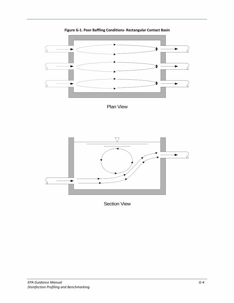
EPA Guidance Manual G-4 Disinfection Profiling and Benchmarking
Figure G-1. Poor Baffling Conditions- Rectangular Contact Basin
Plan View
Section View

EPA Guidance Manual G-5 Disinfection Profiling and Benchmarking
Figure G-2. Average Baffling Conditions- Rectangular Contact Basin
Plan View
Section View

EPA Guidance Manual G-6 Disinfection Profiling and Benchmarking
Superior baffling conditions are demonstrated by the flow pattern and physical characteristics of the basin shown in Figure G-3. The inlet to the basin consists of submerged, target-baffled ports. This inlet design serves to reduce the velocity of the incoming water and distribute it uniformly throughout the basin’s cross-section. The outlet structure is a sharp-crested weir that extends for the entire width of the contact basin. This type of outlet structure will reduce short circuiting and decrease the dead space fraction of the basin, although the overflow weir does create some dead space at the lower corners of the effluent end.
Figure G-3. Superior Baffling Conditions- Rectangular Contact Basin
Plan View
Section View
The plan and section of a circular basin with poor baffling conditions, which can be attributed to flow short circuiting from the center feed well directly to the effluent trough are shown in Figure G-4. Short circuiting occurs in spite of the outlet weir configuration because the center feed inlet is not baffled. The inlet flow distribution is improved somewhat in Figure G-5 by the addition of an annular ring baffle at the inlet which causes the inlet flow to be distributed throughout a greater portion of the basin’s available volume. However, the baffling conditions in this contact basin are only average because the inlet center feed arrangement does not entirely prevent short circuiting through the upper levels of the basin.

EPA Guidance Manual G-7 Disinfection Profiling and Benchmarking
Figure G-4. Poor Baffling Conditions- Circular Contact Basin
Plan View
Section View

EPA Guidance Manual G-8 Disinfection Profiling and Benchmarking
Figure G-5. Average Baffling Conditions- Circular Contact Basin
Plan View
Section View
Superior baffling conditions are attained in the basin configuration shown on Figure G-6 through the addition of a perforated inlet baffle and submerged orifice outlet ports. As indicated by the flow pattern, more of the basin’s volume is utilized due to uniform flow distribution created by the perforated baffle. Short circuiting is also minimized because only a small portion of flow passes directly through the perforated baffle wall from the inlet to the outlet ports.

EPA Guidance Manual G-9 Disinfection Profiling and Benchmarking
Figure G-6. Superior Baffling Conditions- Circular Contact Basin
Plan View
Section View
G.5 Additional Considerations
Flocculation basins and ozone contactors represent water treatment processes with slightly different characteristics from those presented in Figures G-1 through G-6 because of the additional effects of mechanical agitation and mixing from ozone addition, respectively. Studies by Hudson (1975) indicated that a single-compartment flocculator had a T10/T value less than 0.3, corresponding to a dead space zone of about 20 percent and a very high mixed flow zone of greater than 90 percent. In this study, two four-compartment flocculators, one with and the other without mechanical agitation, exhibited T10/T values in the range of 0.5 to 0.7. This observation indicates that not only will compartmentation result in higher T10/T values through better flow distribution, but also that the effects of agitation intensity on T10/T are reduced where sufficient baffling exists. Therefore, regardless of the extent of agitation, baffled flocculation basins with two or more compartments should be considered to possess average baffling conditions (T10/T = 0.5), whereas unbaffled, single-compartment flocculation basins are characteristic of poor baffling conditions (T10/T = 0.3).
EPA Guidance Manual G-10 Disinfection Profiling and Benchmarking
Similarly, multiple stage ozone contactors are baffled contact basins which show characteristics of average baffling conditions. Single stage ozone contactors should be considered as being poorly baffled. However, circular turbine ozone contactors may exhibit flow distribution characteristics that approach those of completely mixed basins, with a T10/T of 0.1, as a result of the intense mixing.
In many cases, settling basins are integrated with flocculators. Data from Hudson (1975) indicates that poor baffling conditions at the flocculator/settling basin interface can result in backmixing from the settling basin to the flocculator. Therefore, settling basins that have integrated flocculators without effective inlet baffling should be considered as poorly baffled, with a T10/T of 0.3, regardless of the outlet conditions, unless intra-basin baffling is employed to redistribute flow. If intra-basin and outlet baffling is utilized, then the baffling conditions should be considered average with a T10/T of 0.5.
Filters are special treatment units because their design and function is dependent on flow distribution that is completely uniform. Except for a small portion of flow that short circuits the filter media by channeling along the walls of the filter, filter media baffling provides a high percentage of flow uniformity and can be considered superior baffling conditions for the purpose of determining T10. As such, the T value can be obtained by subtracting the volume of the filter media, support gravel, and underdrains from the total volume and calculating the TDT by dividing this volume by the flow through the filter (check with the state on what volume may be allowed in a filter). The TDT may then be multiplied by using a factor of 0.7, corresponding to superior baffling conditions, to determine the T10 value.
G.6 Conclusions
The recommended T10/T values and examples are presented as a guideline for use by the state in determining T10. Conditions that are combinations or variations of the above examples may exist and warrant the use of intermediate T10/T values such as 0.4 or 0.6. As more data on tracer studies become available, specifically correlations between other physical characteristics of basins and the flow distribution efficiency parameters, further refinements to the T10/T fractions, and definitions of baffling conditions may be appropriate.
G.7 References
Hudson, H.E., Jr. 1975. Residence Times in Pretreatment. Journal AWWA, 67(1): 45-52.
Marske, D.M. and J.D. Boyle. 1973. Chlorine Contact Chamber Design – A Field Evaluation. Water and Sewage Works, January, pp. 70-77.
USEPA. March 1991. Guidance Manual for Compliance with the Filtration and Disinfection Requirements for Public Water Systems using Surface Water Sources. Washington, D.C.

EPA Guidance Manual H-1 Disinfection Profiling and Benchmarking
Appendix H — Conservative Estimate, Interpolation and Regression Method Examples In some instances, the collected data for the disinfection profile will not coincide exactly with the values in the CT tables. The following examples present three methods on how to obtain CT99.9 values. PWSs that plan to use any of these methods should check with their state to determine if the desired method is acceptable.
Example H-1. Conservative Estimate Example for Obtaining CT99.9
This example will demonstrate one method, Conservative Estimate, for obtaining CT99.9 when collected data values are between values on the CT table. In this example, a conventional filtration treatment system adds chlorine prior to the clearwell and it was required to create a profile. The PWS was required to determine the Giardia and virus log inactivation achieved through disinfection. This example walks through the steps taken to determine the log inactivation for Giardia.
A. Determine the required CT99.9 necessary to obtain 3-log Giardia inactivation.
The required CT value for 3-log Giardia inactivation (CT99.9) may be obtained using CT Table B-1 in Appendix B, CT Values for 3-Log Inactivation of Giardia Cysts by Free Chlorine.
Step 1. Round the temperature value.
Since the temperature of 6°C is not shown in the table, the next lowest temperature on the table, 5°C, is used to obtain a conservative estimate of CT99.9. The lower temperature value was chosen since chlorine is less effective at lower temperatures.
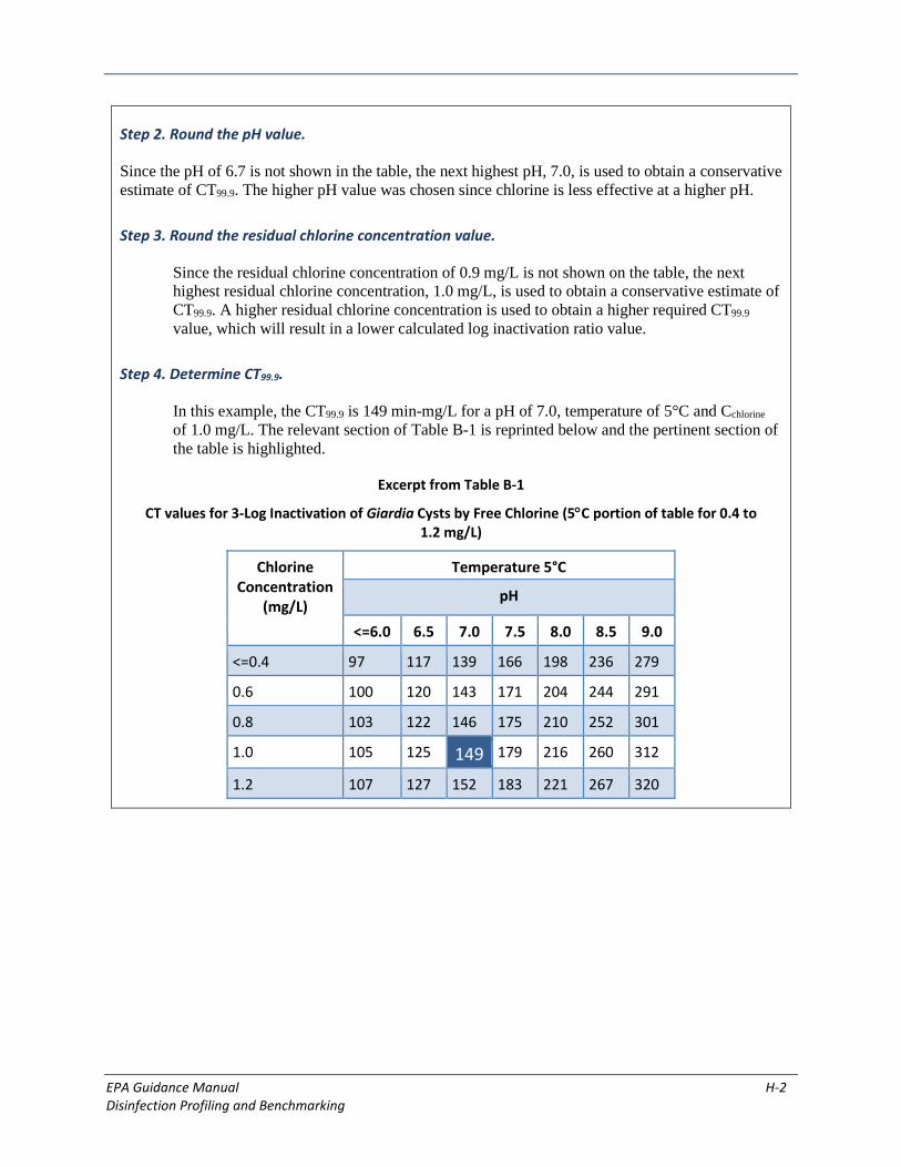
EPA Guidance Manual H-2 Disinfection Profiling and Benchmarking
Step 2. Round the pH value.
Since the pH of 6.7 is not shown in the table, the next highest pH, 7.0, is used to obtain a conservative estimate of CT99.9. The higher pH value was chosen since chlorine is less effective at a higher pH.
Step 3. Round the residual chlorine concentration value.
Since the residual chlorine concentration of 0.9 mg/L is not shown on the table, the next highest residual chlorine concentration, 1.0 mg/L, is used to obtain a conservative estimate of CT99.9. A higher residual chlorine concentration is used to obtain a higher required CT99.9
value, which will result in a lower calculated log inactivation ratio value.
Step 4. Determine CT99.9.
In this example, the CT99.9 is 149 min-mg/L for a pH of 7.0, temperature of 5°C and Cchlorine of 1.0 mg/L. The relevant section of Table B-1 is reprinted below and the pertinent section of the table is highlighted.
Excerpt from Table B-1
CT values for 3-Log Inactivation of Giardia Cysts by Free Chlorine (5°C portion of table for 0.4 to 1.2 mg/L)
Chlorine Concentration
(mg/L)
Temperature 5°C
pH
<=6.0 6.5 7.0 7.5 8.0 8.5 9.0
<=0.4 97 117 139 166 198 236 279
0.6 100 120 143 171 204 244 291
0.8 103 122 146 175 210 252 301
1.0 105 125 149 179 216 260 312
1.2 107 127 152 183 221 267 320
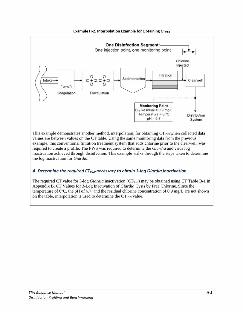
EPA Guidance Manual H-3 Disinfection Profiling and Benchmarking
Example H-2. Interpolation Example for Obtaining CT99.9
This example demonstrates another method, interpolation, for obtaining CT99.9 when collected data values are between values on the CT table. Using the same monitoring data from the previous example, this conventional filtration treatment system that adds chlorine prior to the clearwell, was required to create a profile. The PWS was required to determine the Giardia and virus log inactivation achieved through disinfection. This example walks through the steps taken to determine the log inactivation for Giardia.
A. Determine the required CT99.9 necessary to obtain 3-log Giardia inactivation.
The required CT value for 3-log Giardia inactivation (CT99.9) may be obtained using CT Table B-1 in Appendix B, CT Values for 3-Log Inactivation of Giardia Cysts by Free Chlorine. Since the temperature of 6°C, the pH of 6.7, and the residual chlorine concentration of 0.9 mg/L are not shown on the table, interpolation is used to determine the CT99.9 value.

EPA Guidance Manual H-4 Disinfection Profiling and Benchmarking
Step 1. Interpolate for CT99.9 at pH of 6.7 at the next lowest temperature of 5°C and the next lowest residual chlorine concentration of 0.8 mg/L.
Excerpt from Table B-1
CT Values for 3-Log Inactivation of Giardia Cysts by Free Chlorine (5°C portion of table for 0.4 to 1.2 mg/L)
Chlorine Concentration
(mg/L)
Temperature 5°C
pH
<=6.0 6.5 7.0 7.5 8.0 8.5 9.0
<=0.4 97 117 139 166 198 236 279
0.6 100 120 143 171 204 244 291
0.8 103 122 146 175 210 252 301
1.0 105 125 149 179 216 260 312
1.2 107 127 152 183 221 267 320
(CT99.9 at pH 7.0) – (CT99.9 at pH 6.5)
pH 7.0 – pH 6.5
= (CT99.9 at pH 6.7) – (CT99.9 at pH 6.5)
pH 6.7 – pH 6.5
146 min-mg/L – 122 min-mg/L
7.0 – 6.5
= (CT99.9 at pH 6.7) – 122 min-mg/L
6.7 – 6.5
24 min-mg/L
0.5
= (CT99.9 at pH 6.7) – 122 min-mg/L
0.2
24 min-mg/L x 0.2
0.5
= (CT99.9 at pH 6.7) –122 min-mg/L
9.6 min-mg/L = (CT99.9 at pH 6.7) – 122 min-mg/L
CT99.9 at pH 6.7 = 9.6 min-mg/L + 122 min-mg/L
CT99.9 at pH 6.7 = 131.6 min-mg/L

EPA Guidance Manual H-5 Disinfection Profiling and Benchmarking
Step 2. Interpolate for CT99.9 at pH of 6.7 at the next highest temperature of 10°C and the next lowest residual chlorine concentration of 0.8 mg/L.
Excerpt from Table B-1
CT Values for 3-Log Inactivation of Giardia Cysts by Free Chlorine (10°C portion of table for 0.4 to 1.2 mg/L)
Chlorine Concentration
(mg/L)
Temperature 10°C
pH
<=6.0 6.5 7.0 7.5 8.0 8.5 9.0
<=0.4 73 88 104 125 149 177 209
0.6 75 90 107 128 153 183 218
0.8 78 92 110 131 158 189 226
1.0 79 94 112 134 162 195 234
1.2 80 95 114 137 166 200 240
(CT99.9 at pH 7.0) – (CT99.9 at pH 6.5)
pH 7.0 – pH 6.5
= (CT99.9 at pH 6.7) – (CT99.9 at pH 6.5)
pH 6.7 – pH 6.5
110 min-mg/L – 92 min-mg/L
7.0 – 6.5
= (CT99.9 at pH 6.7) – 92 min-mg/L
6.7 – 6.5
18 min-mg/L
0.5
= (CT99.9 at pH 6.7) – 92 min-mg/L
0.2
18 min-mg/L x 0.2
0.5
= (CT99.9 at pH 6.7) – 92 min-mg/L
7.2 min-mg/L = (CT99.9 at pH 6.7) – 92 min-mg/L
CT99.9 at pH 6.7 = 7.2 min-mg/L + 92 min-mg/L
CT99.9 at pH 6.7 = 99.2 min-mg/L

EPA Guidance Manual H-6 Disinfection Profiling and Benchmarking
Step 3. Interpolate for CT99.9 at pH of 6.7, temperature of 6°C, and the next lowest residual chlorine concentration of 0.8 mg/L.
The table below summarizes the CT99.9 values determined at a pH of 6.7, residual chlorine concentration of 0.8 mg/L and temperatures of 5°C and 10°C.
pH = 6.7
Chlorine Concentration
Temperature
5°C 10°C
0.8 mg/L 131.6 min-mg/L 99.2 min-mg/L
(CT99.9 at 10°C) – (CT99.9 at 5°C)
10°C – 5°C
= (CT99.9 at 6°C) – (CT99.9 at 5°C)
6°C – 5°C
99.2 min-mg/L – 131.6 min-mg/L
10°C – 5°C
= (CT99.9 at 6°C) – 131.6 min-mg/L
6°C – 5°C
-32.4 min-mg/L
5°C
= (CT99.9 at 6°C) – 131.6 min-mg/L
1°C
-32.4 min-mg/L x 1°C
5°C
= (CT99.9 at 6°C) – 131.6 min-mg/L
-6.48 min-mg/L = (CT99.9 at 6°C) – 131.6 min-mg/L
CT99.9 at 6°C = -6.48 min-mg/L + 131.6 min-mg/L
CT99.9 at 6°C = 125.1 min-mg/L
CT99.9 at a pH of 6.7, temperature of 6°C, and residual chlorine concentration of 0.8 mg/L is 125.1 min-mg/L.

EPA Guidance Manual H-7 Disinfection Profiling and Benchmarking
Step 4. Repeat steps 1 through 3 at the same pH and temperatures, but with a residual chlorine concentration of 1.0 mg/L.
The results are summarized in the table, below.
pH Temperature (°C)
Residual Chlorine Conc. (mg/L)
CT99.9 (min-mg/L)
6.7 5 1.0 134.6
6.7 10 1.0 101.2
6.7 6 1.0 127.9
CT99.9 at a pH of 6.7, temperature of 6°C, and residual chlorine concentration of 1.0 mg/L is 127.9 min-mg/L.
Step 5. Interpolate for CT99.9 at pH of 6.7, temperature of 6°C, and residual chlorine concentration of 0.9 mg/L.
The table below summarizes the CT99.9 values determined at a pH of 6.7, temperature of 6°C, and residual chlorine concentrations of 0.8 mg/L and 1.0 mg/L.
pH = 6.7
Temperature Chlorine Residual Conc.
0.8 mg/L 1.0 mg/L
6°C 125.1 min-mg/L 127.9 min-mg/L
(CT99.9 at 1.0 mg/L) – (CT99.9 at 0.8 mg/L)
1.0 mg/L – 0.8 mg/L
= (CT99.9 at 0.9 mg/L) – (CT99.9 at 0.8 mg/L)
0.9 mg/L – 0.8 mg/L
127.9 min-mg/L – 125.1 min-mg/L
1.0 mg/L – 0.8 mg/L
= (CT99.9 at 0.9 mg/L) – 125.1 min-mg/L
0.9 mg/L – 0.8 mg/L
2.8 min-mg/L
0.2 mg/L
= (CT99.9 at 0.9 mg/L) – 125.1 min-mg/L
0.1 mg/L

EPA Guidance Manual H-8 Disinfection Profiling and Benchmarking
2.8 min-mg/L x 0.1 mg/L
0.2 mg/L
= (CT99.9 at 0.9 mg/L) – 125.1 min-mg/L
1.4 min-mg/L = (CT99.9 at 0.9 mg/L) – 125.1 min-mg/L
CT99.9 at 0.9 mg/L = 1.4 min-mg/L + 125.1 min-mg/L
CT99.9 at 0.9 mg/L = 126.5 min-mg/L
CT99.9 at a temperature of 6°C, pH of 6.7, and residual chlorine concentration of 0.9 mg/L is 126.5 min-mg/L.
Note that this CT99.9 value of 126.5 min-mg/L is substantially lower than the value of 149 min-mg/L obtained through the conservative estimate in Example H-1. Making use of this interpolation approach will allow the PWS to demonstrate compliance at a lower level of disinfection dose.

EPA Guidance Manual H-9 Disinfection Profiling and Benchmarking
Example H-3. Regression Example for Obtaining CT99.9 when Free Chlorine is Used as the Disinfectant
The regression method is useful for calculating CT99.9 when using free chlorine as a disinfectant for a long historical data set of pH, temperature, and residual disinfectant concentrations. Instead of having to look up CT values weekly, the regression method allows the operator to simply use a formula that is a function of pH, temperature, and residual disinfectant concentration.
An empirical model was developed by Smith et al. (1995), that directly predicts CT values that are equal to or greater than the original CT values in the SWTR over the entire range of variables covered in the Guidance Manual for Compliance with the Filtration and Disinfection Requirements for Public Water Systems Using Surface Water Sources (USEPA, March 1991). The equations below can be used to directly compute CT values for chlorine inactivation:
CT99.9 = (0.353 x I)(12.006 + e(2.46 - 0.073 x temp + 0.125 x C + 0.389 x pH)) [for temperatures <12.5°C]
CT99.9 = (0.361 x I)(-2.261 + e(2.69 - 0.065 x temp + 0.111 x C + 0.361 x pH)) [for temperatures ≥12.5°C]
Where: I = 3 (the number of log inactivation credits required) temp = temperature in degrees Celsius C = residual chlorine concentration in mg/L pH = the pH value
The following example walks through the steps taken to determine the log inactivation credits for Giardia using the regression method when free chlorine is the disinfectant.
A. Determine the required CT99.9 necessary to obtain 3-log Giardia inactivation.
The regression method is used to determine the CT99.9 value.
Step 1. Determine whether the temperature is above, below, or equal to 12.5°C.
Once again, using the same monitoring data from the previous examples, the temperature is 6°C. Therefore, the first equation listed above will be used to determine the required CT value for 3-log Giardia inactivation (CT99.9).
Step 2. Determine CT99.9.
With a pH of 6.7 and residual chlorine concentration of 0.9 mg/L during peak hourly flow, calculate the CT99.9 using the regression method as follows: CT99.9 = (0.353 x I)(12.006 + e(2.46 - 0.073 x temp + 0.125 x C + 0.389 x pH))
CT99.9 = (0.353 x 3)(12.006 + e(2.46 - 0.073 x 6 + 0.125 x 0.9 + 0.389 x 6.7))
CT99.9 = 134 min-mg/L
This value is between the values obtained from the other two methods (conservative method: 149 min-mg/L; linear interpolation: 126.5 min-mg/L).

EPA Guidance Manual H-10 Disinfection Profiling and Benchmarking
References
Smith D.B., R.M. Clark, B.K. Pierce, and S. Regli. 1995. An Empirical Model for Interpolating C*T Values for Chlorine Inactivation of Giardia lamblia. J. Water SRT- Aqua. 44(5):203-211.
USEPA. March 1991. Guidance Manual for Compliance with the Filtration and Disinfection Requirements for Public Water Systems Using Surface Water. Washington, D.C.