distributed inference for network localization using radio ...ijwang/pub/lucarellietalewsn.pdf ·...

Distributed Inference for Network Localization

Using Radio Interferometric Ranging

Dennis Lucarelli1, Anshu Saksena1, Ryan Farrell1,2, and I-Jeng Wang1

1 Applied Physics Laboratory, Johns Hopkins University, Laurel, MD2 Computer Science Department, University of Maryland, College Park, MD

Abstract. A localization algorithm using radio interferometric mea-surements is presented. A probabilistic model is constructed thataccounts for general noise models and lends itself to distributed computa-tion. A message passing algorithm is derived that exploits the geometryof radio interferometric measurements and can support sparse networktopologies and noisy measurements. Simulations on real and simulateddata show promising performance for 2D and 3D deployments.

1 Introduction

Self-localization is a fundamental, yet not completely solved, problem in thedesign and deployment of sensor networks. It is fundamental because sensornetworks are envisioned to provide visibility and monitoring with inexpensivedevices in GPS denied areas. Despite many localization algorithms and improve-ments in device hardware, one can argue that the problem is not completelysolved since no single method has been widely adopted for such a fundamen-tal problem. Most notably, there is a need for a localization system capable ofhandling the multipath effects encountered indoors and in dense urban areas.The main impediment to the creation of such a system is an effective means ofobtaining range measurements in a multipath environment and the developmentof localization algorithms that can account for these effects.

Various technologies such as ultrasound/RF TDOA ranging [1], acoustic TOA(e.g. [2]), and received radio signal strength (e.g. [3]), have been proposed anddemonstrated for acquiring pairwise distance estimates. Broadly speaking anddespite the ingenuity of these approaches, these methods are plagued by shortrange, poor precision, or the requirement of an ancillary system devoted just toranging. Given these limitations, researchers have proposed methods for networklocalization that do not rely on ranging at all. These so-called range free methods,see for example [4,5,6], use either a camera system or in the case of [5] a steerablelaser to localize the nodes. Again, these solutions require additional hardwareand calibration to solve the problem.

A recent breakthrough has changed the localization landscape considerably.Researchers at Vanderbilt University have proposed and demonstrated a surpris-ingly simple, yet powerful, method for ranging using only the radio that producescentimeter ranging accuracy at ranges up to 160 meters [7,8]. This technique,

R. Verdone (Ed.): EWSN 2008, LNCS 4913, pp. 52–73, 2008.c© Springer-Verlag Berlin Heidelberg 2008

Distributed Inference for Network Localization 53

known as radio interferometric ranging, exploits electromagnetic interference toobtain an observable that is a function of the locations of four nodes sensors(known here as a quad) involved in the measurement. As such, it does not di-rectly produce pairwise distance measurements, but rather a linear combinationof four of the possible six pairwise distances. This fact renders localization algo-rithms that rely on pairwise distances unable to capitalize on this new technique.Perhaps the most remarkable feature of this technique is that it can be imple-mented with coarse time synchronization on inexpensive radios found on widelyavailable sensor network devices.

In this paper, we propose a distributed algorithm for network localizationusing radio interferometric ranging. We derive and exploit the geometry under-lying the ranging technique that enables the algorithm. In the next section weshow how the location of a node is constrained conditional on the location ofthe three other nodes involved in the ranging measurement. We show that, inthe two dimensional case, knowing the location of three nodes constrains thefourth to a branch of a hyperbola. By taking two independent measurementson those four nodes, one can obtain another distinct hyperbola thus furtherconstraining the nodes location to lie on the intersection of these conics. Giventhat the knowledge of three nodes and two independent interferometric rangemeasurements (RIMs) reduces the uncertainty of the fourth node to just oneor two intersection points, it seems plausible that a multilateration procedurecan be derived akin to trilateration in systems with pairwise measurements. In-deed, assuming a 2D deployment with four anchor nodes1 and a sensor withinRIM’s range of the four anchors, the unknown node can participate in up tothree separate independent quads [8]. Further assuming that for each quad twoindependent measurements are obtained, a set of intersections points can becomputed for the unknown sensor and this set of points could then potentiallybe used to determine the location of the unknown node.

In contrast, we adopt a probabilistic approach. Given the nonlinear relation-ships defined by the ranging procedure, their resulting uncertainty and our ul-timate goal of developing a robust means of network localization in multi-pathenvironments, a nonparametric probabilistic approach is preferred. We embedthe underlying geometry in a flexible probabilistic model that lends itself todistributed computation. With the appropriate definition of the model, the dis-tributed inference algorithm, known as belief propagation, in a sense, “comes forfree.” In this regard, our approach is very much in the spirit of Ihler et al. [9],but adapted to the subtleties of dealing with radio interferometric ranging.

2 Conditional Geometry of Radio InterferometricMeasurements

The functional form of the radio interferometric range measurement presents aunique challenge in designing a distributed localization algorithm. On a set of1 Three anchors will not suffice, since, in the general case, the uncertainty of the

unlocalized node can only be reduced to two distinct intersection points.

54 D. Lucarelli et al.

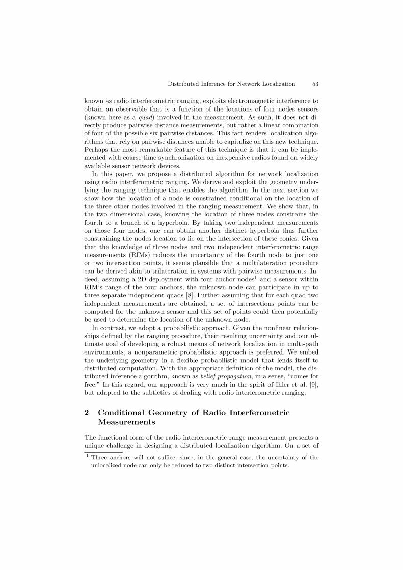
Fig. 1. Radio interferometric measurement

four sensors labeled T, U, V, and W, after post processing the RIM is givenby [7,8]

dTUV W := ||T −W || − ||U −W || + ||U − V || − ||T − V || + η (1)

where η represents an additive noise term. However, if three of the four nodesinvolved in the measurement are known, say for example, {T, V,W}, the mea-surement reduces to a quadratic equation in the coordinates of the unknownnode,

dTUV W = − ||U −W || + ||U − V || + k′ + η (2)

where k′ is the constant given by ||T −W || − ||T − V || . As is evident, in twodimensions the locus of points satisfying this equation is a conic section. Specif-ically, by setting dTUV W = k∗ and neglecting the noise term for a moment, theequation

k = k∗ − k′ = − ||U −W || + ||U − V || (3)

describes the location of node U conditional on the measurement and the loca-tions of the nodes {T, V,W} .

Equation 3 defines one branch of a hyperbola with foci at the points {V,W} .There are two independent RIMs on four nodes [8] corresponding to two dis-tinct hyperbolae, thus the uncertainty of the unknown sensor location can befurther reduced by taking an additional measurement. For example, the measure-ment dTV UW := ||T −W || − ||V −W || + ||U − V || − ||T − U || defines a secondhyperbola with the unknown node location at the intersection points of the hy-perbolae defined by the measurements {dTUV W , dTV UW } . Figure 2 depicts the


T

U

V

W

T

U

V

W

T

UV

W

T

UV

W

Fig. 2. Intersection points of hyperbolae defined by two independent RIMs

scenario with the unknown sensor cycling through all four possibilities with thetwo measurements fixed. From the figure we can get a feel for the sensitivityof the intersections to the input data. For example, the figure in the upperleft quadrant (where T is the unknown node location) we see that not only twointersection points exist but also the hyperbolae almost coincide on the arc whereT lies. Clearly this geometry is very susceptible to noise in the input data andhints to the difficulty in crafting a localization algorithm for ad-hoc networkswith interferometric ranging. A favorable geometry is depicted in the lower leftquadrant, where the hyperbolae intersect in a unique isolated point V .

Computing the intersection points of two conics, in general, requires solving aquartic equation that does not admit a convenient closed form solution. However,if the hyperbolae share a common focus, as is the case for the measurement set{dTUV W , dTV UW }, this system reduces to a quadratic equation and the intersec-tion points can be computed exactly and efficiently. For example, the location ofsensor V is a common focus of the hyperbolae defined by dTUV W and dTV UW ,if sensor U is the unknown node.

Since a literature survey did not uncover the procedure for computing in-tersection points of conics sharing a focus, a derivation is presented here. If atranslation and rotation are applied to bring the common focus to the originand the other focus of one of the hyperbolae to the x-axis, then the equation inpolar coordinates of the hyperbola with both foci on the x-axis is

r1(θ) =m1

e1 cos(θ) − 1, (4)

where

m1 = ||f1||e21 − 12e1

, (5)


e1 is the eccentricity of the hyperbola and ||f1|| is the distance between the twofoci. If the angle of elevation of the semimajor axis of the second hyperbola is φ,then the equation of that hyperbola is

r2(θ) =m2

e2 cos(θ − φ) − 1, (6)

where

m2 = ||f2||e22 − 12e2

, (7)

e2 is the eccentricity and ||f2|| is the distance between the foci. These expressionsdescribe both branches of the hyperbolae. Once we find the intersections, we willeliminate those involving the extraneous branches. With the common focus at theorigin, there is a range of values within arctan(

√e2 − 1) of the positive direction

of the semimajor axis (i.e., θ = 0 for the first hyperbola, θ = φ for the second)for which there are two points of the hyperbola – one corresponding to a positivevalue of ri and lying on one branch of the hyperbola, and one corresponding toa negative value of ri for θ halfway around the circle on the other branch. Inorder to find all intersections of the hyperbolae, we need to set r1(θ) = r2(θ)to find intersections of portions of each hyperbola with the same sign of ri and−r1(θ + π) = r2(θ) to find intersections of the negative part of one hyperbolawith the positive part of the other.

These equalities each yield a quadratic expression in cos(θ) whose standardform coefficients are:

a1 =(e1m1

− e2m2

)2

+ 2e1e2m1m2

(1 − cos (φ)) (8)

b1 = 2(e1m1

− e2m2

cos (φ)) (

1m2

− 1m1

)(9)

c1 =(

1m2

− 1m1

)2

−(e2m2

)2 (1 − cos2 (φ)

)(10)

for the first equality and

a2 =(e1m1

− e2m2

)2

+ 2e1e2m1m2

(1 − cos (φ)) (11)

b2 = 2(e1m1

− e2m2

cos (φ)) (

1m1

+1m2

)(12)

c2 =(

1m1

+1m2

)2

−(e2m2

)2 (1 − cos2 (φ)

)(13)

for the second. If the discriminant di = b2i − 4aici is negative, zero, or posi-tive, that equality has no solutions, one solution, or two solutions, respectively.Therefore, the total number of intersections of the hyperbolae can be anywherebetween zero and four. If there are solutions, they are given by:

cos(θi) =−bi ±

√di

2ai(14)


for i = 1 or 2 indicating which hyperbolic intersection equality we are evaluating.In order to solve for θi, we must calculate sin(θi) as well to ensure we determinethe correct quadrant.

sin(θ1) =cos(θ1)(e1m2 − e2m1 cos(φ)) −m2 +m1

e2m1 sin(φ)(15)

sin(θ2) =cos(θ2)(e1m2 − e2m1 cos(φ)) +m1 +m2

e2m1 sin(φ)(16)

The solutions for θi then can be calculated by taking the arctangent of thequotient of the sine and cosine, maintaining the correct quadrant. We eliminatethose values that are outside the range of values for the branch of each hyperbolathat correspond to the measurement constraint. After doing so we will have zero,one, or two values of θi remaining. Although for the most part we will have anonzero number of intersections remaining since the nodes are embedded in thespace and the measurements are derived from their positions, noise in the mea-surements can occasionally cause a situation where no intersections are possible.This indicates that the positions of at least one of the three foci is inconsistentwith the measurements. When intersections remain, plugging their values backinto Eq. (6) and rotating and translating back to the original coordinate systemgives us the possible locations of the unknown sensor node.

The radio interferometric technique is not restricted to two dimensions. More-over, the geometry associated with the measurements generalizes as well. In the3D case, the conditional uncertainty of a node given the location of the three oth-ers is a hyperboloid. Two RIMs reduce the uncertainty to the intersection curveof the hyperboloids. Again if two hyperboloids share a common focus, solvinga simple quadratic equation leads to an analytic parameterization of the inter-section curve [10]. It turns out that this intersection curve is a hyperbola or anellipse. Examples of the geometry of 3D RIMs is depicted in Figure 3 where a to-tal of four measurements are taken, two generating a hyperbolic intersection and

Fig. 3. Intersection curves of hyperboloids defined by RIMs in 3D


the other two generating an elliptical intersection. The location of the unknownsensor lies on the intersection of these two curves as depicted in the figure.

3 Problem Formulation

In the preceding section, the geometric intuition behind the proposed algorithmwas outlined. These considerations, even in the 2D case, do not suffice to design arobust, scalable localization algorithm. Our approach embeds the multilaterationprimitive into a probabilistic model that allows for soft assignments of the sensorlocations that are iteratively refined over time.

In addition to the nonlinearity introduced by the form of the interferometricmeasurement, noise and errors from a variety of sources affect the measurementvalue [7]. These sources of error, such as multipath effects, carrier frequency inac-curacy, time synchronization error and signal processing errors, are modeled by anoise distribution in our algorithm. These errors manifest in the post processingof the interferometric measurements as a possible error that is a multiple of thewavelength of the carrier frequency. This distribution can therefore be modeledas a small Gaussian mixture with components centered at integer multiples ofthe wavelength of the carrier frequency. It has been shown that iterative filter-ing techniques can be applied to the radio interferometric ranging procedure toproduce high precision range estimates in a mild multipath environment thateffectively remove the non-Gaussian nature of the errors [8]. Though it has notbeen explicitly demonstrated, an RSSI technique such as radio interferometrywill likely suffer performance degradation in a high multi-path environment suchas indoors or in a dense urban area. Our approach attempts to explicitly handlethe effects of ranging error by associating a random variable to each sensor loca-tion and defining the joint distribution of the sensor locations that incorporatesthe intrinsic geometry of the radio interferometry technique.

The formalism used to capture the uncertainty and the measurement modelis a probabilistic graphical model. Let X = {x1, x2 . . . xn} be a collection ofrandom variables. A graphical model is a factored representation of the jointdistribution over X defined by a set of potential functions ψ(·) that encode thecoupling among the variables and an undirected graph that represents the notionof conditional independence among sets of random variables. Given a graph andset of potential functions, the joint distribution can be written as

p(x1, x2, . . . , xn) ∝∏c∈C

ψc(xc) (17)

where C is the set of fully connected subsets or cliques of the graph and xc = {xu :xu ∈ c}. Graphical models are often employed for problems where the cliquescan be restricted to pairs of nodes and the joint distribution given measurementsis given by

p(x1, x2, . . . , xn|D) ∝∏

(u,v)∈Eψuv(xu, xv, duv)

∏u

ψu(xu, du) (18)


where E is the set of edges in the graph and D denotes the entire set of mea-surements , duv, du ∈ D and ψ(xu, du) is a local potential function that is usedto capture any a priori knowledge for a node or to model a local measurement.

The graphical representation of the joint distribution has inspired many infer-ence algorithms that exploit this graphical structure to achieve greater efficiency.An iterative message passing algorithm known as belief propagation is one of thebest known of these methods for computing marginal distributions due to itssimplicity and excellent empirical results on high dimensional problems. Forproblems involving spatial data in ad-hoc sensor networks, one can exploit theanalogy of a communications graph, where an edge signifies a communicationchannel between sensors, and identify these two graphical representations to de-velop a probabilistic model for fusing measurement data that includes a simplemessage passing algorithm for performing inference on that model.

For continuous systems with pairwise couplings, the belief propagation updateequations are given by an expression for computing a message from node u tonode v , denoted muv(xv) , and an expression for computing the belief at a node,βv , which is an estimate of the marginal distribution of the random variable xv .At iteration n, the message update is given by

mnuv(xv) ∝

∫ψ(xu, xv)ψ(xu)

∏(w,u)∈E\(v,u)

mn−1wu (xu) dxu (19)

Note that the message sent from node xv in the previous iteration is excludedfrom the message product for consistency of the marginalization procedure.

Roughly speaking, Eq. (19) represents node u’s belief about the marginalof node v given its measurements and the messages from its neighbors in thegraph from the previous iteration. Fusion of these messages to approximate itsmarginal is achieved by simply taking the product of received messages and thelocal potential function,

βn(xv) ∝ ψ(xv)∏

(w,v)∈Emn

wv(xv) (20)

In the context of sensor networks, the attraction of belief propagation in a graph-ical model is evident since it is a simple way to perform global inference usinglocal communications and distributed computation. However, the correctness ofbelief propagation is not guaranteed unless one restricts the graphical structureto a tree. Fortunately, the so called loopy version of belief propagation, whereone carries out the message and fusion updates of Eqs. (19) and (20) withoutregard to the existence of loops in the graph, has shown excellent empirical per-formance in a variety of settings. There has been some progress in understandingthe convergence of loopy belief propagation. The most useful characterization forthis discussion is that if the loopy algorithm converges, it will converge to fixedpoints of the so called Bethe free energy [11]. Alternatively, one may always ag-gregate random variables into a junction tree and conduct message passing onthat tree to perform inference exactly; however, the complexity of the algorithm


is exponential in a graphical property of the junction tree known as the treewidth.

As may be intuitively obvious, a graphical model formulation of the networklocalization problem with interferometric ranging will not have pairwise cou-plings since the variables are coupled by the measurement that involves fournodes to obtain one observable. The joint distribution factors according to thiscoupling and is given by

p(x1, . . . xn|D) ∝∏

t

ψ(xt)∏

(tuvw)∈Qψ(xt, xu, xv, xw, dTUV W ) (21)

where Q is the set of quads in the graph.There are a number of ways to define higher order belief propagation. One

method, as mentioned above, is to aggregate variables into a junction tree. Thistechnique has been extended for distributed inference problems in sensor net-works with lossy communications in [12]. In this work, we follow a derivationobtained by minimizing the Bethe free energy in a manner analogous to the casewith pairwise potential functions [13].

Let Tw be the set of index triples that share an interferometric range mea-surement with node xw. Formally, if (tuv) ∈ Tw, we can express the messagefrom the set {xt, xu, xv} to node xw , denoted mn

tuvw(xw) , as

mntuvw(xw) ∝

∫ψ(xt)ψ(xu)ψ(xv)ψ(xt, xu, xv, xw)

∏(qrs)∈Tv\(tuw)

mn−1qrsv(xv)

∏(qrs)∈Tu\(tvw)

mn−1qrsu(xu)

∏(qrs)∈Tt\(uvw)

mn−1qrst (xt) dxtdxudxv (22)

Analogous to the pairwise case, the estimate of the marginal is simply the prod-uct of the incoming messages with the local potential function

βn(xw) ∝ ψ(xw)∏

(tuv)∈Tw

mntuvw(xw) (23)

While being functionally simple, the expression defining the messages suffersfrom two serious drawbacks. First, the integral is clearly intractable for denselyconnected networks of resource constrained devices such as sensor networks. Wedefer the discussion of this important consideration until the next section wherea suitable approximation technique is presented. The second drawback of suchan expression, which is clearly exacerbated in the case of four node couplings, isthe complexity and coordination required among the sensors to implement themessage passing. While being decentralized, a direct implementation of an algo-rithm utilizing (22) would be a poor distributed algorithm due to the complexityof the message passing. For example, as depicted in Figure 4, to pass a messagefrom the triple (ijk) ∈ Tl to xl , the sending triple would have to elect a leadernode to recieve the individual nodes’ contributions and perform the product andintegral in (22). Following the approach suggested in [14,9,15], we can simplify


mni jkl(xl)

x j

xnxl

xk

xi

xm

mn−1jmnk(xk)

Fig. 4. Higher-order belief propagation message passing

the message passing to broadcast communications at the cost of local memory.To see this, note that the beliefs (23) contain much of the information requiredto form the message (22), except for the four variable potential function and thecorrection required for consistency. Thus, given the measurements, each nodecan reconstruct the incoming messages from the collection of beliefs broadcastby nodes who share measurements with it by forming,

mntuvw(xw) ∝

∫ψ(xt, xu, xv, xw)

βn−1(xt)βn−1(xu)βn−1(xv)mn−1

uvwt(xt)mn−1tvwu(xu)mn−1

tuwv(xv)dxtdxudxv .

(24)In this formulation, a node updating its belief reconstructs the incoming mes-sages by using neighboring nodes’ beliefs and forming (24). These messages arethen used in the node’s belief update. It then calculates messages it would sendto each of its neighbors using (22) and stores them locally to use in (24) in thenext iteration while broadcasting its newly calculated belief instead of sending{muvwt(xt) ,mtvwu(xu) ,mtuwv(xv)}.

4 Nonparametric Belief Propagation

In the previous section, formal expressions were presented for performing dis-tributed inference over continuously valued random variables. A continuousmodel is favored over a discrete model, arising from a discretization of the sensorfield, for a variety of reasons. First, the resolution of the localization solutionis dictated by the size of the grid and thus the state space of the random vari-able grows quadratically with the precision of the solution. This would forcean intractable summation in the discrete analogue of the BP equation (22).A discrete model also implies a priori knowledge of the size of the field which


cannot be guaranteed for ad-hoc deployments. A Gaussian model is inappro-priate as well, since radio interferometric measurements exhibit non-Gaussianerrors and, as shown previously, two measurements on four nodes restrict thelocalization solution to one or two intersection points of hyperbolae in the twodimensional case, which is a non-linear coupling of the random variables. There-fore a non-Gaussian, non-linear approach is preferred. Despite the advantagesof the non-Gaussian continuous model, at this point we have only exchangedan intractable summation with an intractable integral. The key innovation ofnonparameric belief propagation [16,17] that enables the integration of thesemethods to sensor networks is an efficient technique to stochastically approxi-mate the message products and integral appearing in (22, 23) by sampling basedmethods.

To this end, we pursue a nonparametric approximation of the beliefs andmessages as mixtures of Gaussians,

mtuvw(xw) =N∑i

αiwN (xw, μ

iw, Λ) (25)

where N (x, μ, Λ) is a Gaussian random variable centered at the sample μ andcovarianceΛ, αi

w is the weight of the ith Gaussian component of the mixture, andN is the number samples. Since the product of Gaussian mixtures is a Gaussianmixture and further assuming that the potential function can be modeled as aGaussian mixture, the products appearing in (22, 23) are well defined and againGaussian mixtures, albeit with O(N q) components for products of q messages.If N is large enough to represent the distribution and for q > 2 messages, exactsampling of (22, 23) would be intractable. Several techniques for approximatesampling from Gaussian mixtures were presented in [18]. In our simulations weused an approach from [18] known as mixture importance sampling, though othermethods performed similarly. Covariances are determined by the so-called ruleof thumb, which is simply an estimated weighted variance of the samples.

5 Description of the Algorithm

Given the machinery of nonparametric belief propagation and analytic expres-sions for the intersection sets resulting from the underlying geometry, thedistributed algorithm is relatively straightforward to define. To do so, we mustdefine the probabilistic model specified by the graph and its single and four nodepotential functions. The graph describing the coupling of the random variablesis given by the ad-hoc deployment of the sensor nodes and the radio interfer-ometric measurements collected in the field. Thus for each measurement, wedefine a clique on the four participating nodes. In this work, we also assumethat this graph is contained in the communications graph so that there is a com-munications link between all nodes sharing a measurement. In practice this maynot be the case as it has been demonstrated that interferometric measurementscan be obtained with relatively weak signals that are not of sufficient fidelity


Resulting Update Message

RIM Measurements

T

U

V

W

Nonparametric Beliefs

T

U

VNoise Model

Belief Samples

Conditional Geometry

T

U

V

W

RIM Quad

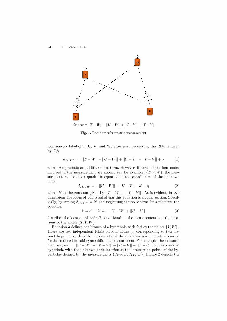
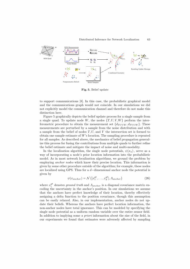
Fig. 5. Belief update

to support communications [8]. In this case, the probabilistic graphical modeland the communications graph would not coincide. In our simulations we didnot explicitly model the communication channel and therefore do not make thisdistinction here.

Figure 5 graphically depicts the belief update process for a single sample froma single quad. To update node W , the nodes {T, U, V,W} perform the inter-ferometric procedure to obtain the measurement set {dTUV W , dTV UW }. Thesemeasurements are perturbed by a sample from the noise distribution and witha sample from the belief of nodes T, U, and V the intersection set is formed toobtain one sample estimate of W ’s location. The sampling procedure is repeatedfor all samples. As described above, the mechanics of belief propagation general-ize this process for fusing the contributions from multiple quads to further refinethe belief estimate and mitigate the impact of noise and multi-modality.

In the localization algorithm, the single node potentials, ψ(xu) , serve as away of incorporating a node’s prior location information into the probabilisticmodel. As in most network localization algorithms, we ground the problem byemploying anchor nodes which know their precise location. This information isgiven by some other procedure outside of the algorithm; for example, these nodesare localized using GPS. Thus for a d−dimensional anchor node the potential isgiven by

ψ(xanchor) = N([xgt

1 , . . . , xgtd ], Λanchor

)(26)

where xgti denotes ground truth and Λanchor is a diagonal covariance matrix en-

coding the uncertainty in the anchor’s position. In our simulations we assumethat the anchors have perfect knowledge of their location, thereby effectivelyassigning a delta function to the position covariance, though this assumptioncan be easily relaxed. Also, in our implementation, anchor nodes do not up-date their beliefs. Whereas the anchors have perfect location information, thenon-anchor nodes have total ignorance. This can be modeled by specifying thesingle node potential as a uniform random variable over the entire sensor field.In addition to implying some a priori information about the size of the field, inour experiments we found that estimates were adversely affected by sampling


error of this uniform distribution. Therefore, we instantiate the single node po-tentials for non anchors as empty. Since the single node potentials serve as priorinformation, empty single node potentials achieve the desired uncertainty butthis choice affects initialization and the scheduling of the message updates. Weaddress this issue in the following section.

The four node potential functions define the coupling given by the interfero-metric measurement. Given a model of the noise distribution, pη we can formallywrite the potential function as

ψ(xt, xu, xv, xw) = pη1 · pη2 where (27)pη1 = pη (dTUV W − (||xt − xw|| − ||xv − xw || + ||xu − xv|| − ||xt − xv||)) (28)pη2 = pη (dTV UW − (||xt − xw|| − ||xu − xw || + ||xu − xv|| − ||xt − xu||)) (29)

Thus given an instantiation of the random variables and the potential functionsdefined as above, the joint distribution (21) expresses its likelihood. In our al-gorithm, these formal expressions are instantiated by the analytic expressionsobtained by solving for the intersection set of the hyperbolae as described in thefollowing.

The algorithm is initialized by performing the radio interferometric rangingprocedure. Currently the coordination and estimation is executed at a base sta-tion [7,8,19]. Frequency and phase estimation is performed at the node level andfrom that information an estimate of the measurement dTUV W can be computed.In this paper, we assume a situation where the range estimates can be obtainedin the network and so that with the following algorithm, the entire localiza-tion procedure is distributed and performed in the network. In this scenario,local messages are sent so that all nodes involved in a measurement receive therange estimate. Also, as described previously, we only consider quads where twoindependent interferometric measurements have been taken. For simplicity, weassume that these are of the form dTUV W and dTV UW .

The expression defining the four node potential function is now made moreconcrete. The messages appearing in (24) are reconstructed at a node accordingto the following. Upon receiving a collection of weighted samples

{βn(xt), βn(xu), βn(xv)} ={(xi

t, αit), (xi

u, αiu), (xi

v , αiv)

}N

i=1(30)

representing a current set of beliefs for which measurements exist, node xw

propagates these samples through the potential function to construct the mes-sage mtuvw . The basic idea is to use the measurements and the three samplepoints to form the intersection set. To this end, the updating node xw uses theordering of the measurement to determine the common focus of the two hyper-bolae (hyperboloids). For example, for the measurements dTUV W and dTV UW

the common focus is xt since we have

dTUV W =∣∣∣∣xi

t − xiw

∣∣∣∣ − ∣∣∣∣xiu − xi

w

∣∣∣∣ +∣∣∣∣xi

u − xiv

∣∣∣∣ − ∣∣∣∣xit − xi

v

∣∣∣∣ (31)

=∣∣∣∣xi

t − xiw

∣∣∣∣ − ∣∣∣∣xiu − xi

w

∣∣∣∣ + kTUV W (32)


and

dTV UW =∣∣∣∣xi

t − xiw

∣∣∣∣ − ∣∣∣∣xiv − xi

w

∣∣∣∣ +∣∣∣∣xi

u − xiv

∣∣∣∣ − ∣∣∣∣xit − xi

u

∣∣∣∣ (33)

=∣∣∣∣xi

t − xiw

∣∣∣∣ − ∣∣∣∣xiv − xi

w

∣∣∣∣ + kTV UW (34)

since using the i-th sample from current beliefs sets {xit, x

iu, x

iv} , the last two

terms in each expression evaluate to constants. Note that the ordering of themeasurement matters. In the interferometric ranging procedure this ordering isdetermined by which nodes are transmitters and which are receivers and there-fore easily obtained and stored in memory. The sample set is translated androtated so that the common focus is at the origin and another focus lies on the xaxis. Now for each measurement a sample is drawn from the noise model ηj ∼ pη

and the constants defining the hyperbolae (hyperboloids) are perturbed by thissample. Thus we have the quadratic equations defining our constraints on thelocation of the updating node as

dTUV W − kTUV W + η1 =∣∣∣∣xi

t − xiw

∣∣∣∣ − ∣∣∣∣xiu − xi

w

∣∣∣∣ (35)

anddTV UW − kTV UW + η2 =

∣∣∣∣xit − xi

w

∣∣∣∣ − ∣∣∣∣xiv − xi

w

∣∣∣∣ . (36)

From the left hand sides of these equations and the samples defining the foci,the intersection set of the hyperbolae (hyperboloids) can be computed. In the 2Dcase, it is possible that the intersection set is a single point, however in generalthe intersection set itself must be sampled to produce the message sample mi

tuvw .Note that this point must now be transformed back to the original coordinatessystem of the input data. Recall that the notation mtuvw denotes the message“sent” from {xt, xu, xv} to xw .

Finally the samples from the intersection set are weighted to complete a faith-ful approximation to (24).

αituvw =

αitα

iuα

ivR(mi

tuvw)muvwt(xt)mvwtu(xu)mwtuv(xv)

. (37)

In the expression defining the weight for the message sample mituvw we have in-

troduced the function R(·) . This function serves to weight samples based on thenotion of range. Because the intersection sets are sensitive to noise in the definingdata, it can be the case that some samples are placed far outside the sensor field.This function limits the impact of these outliers by taking the max distance of thenew sample from the incoming beliefs samples and evaluates an exponentially de-creasing function on that distance. In the 3D case, the notion of maximum rangealso defines intervals to sample the unbounded hyperbola intersection curves sothat only a segment of that hyperbola is ever used in the message update. Thisprocedure is performed for all samples to construct a sample based estimate ofthe message mtuvw ≈

{mi

tuvw, αituvw

}N

i=1. When all messages have been sim-

ilarly constructed, samples are drawn from the message product (23) to formthe estimate of the marginal β(xw) as described in the previous section. Finally,


now that node xw has an updated belief, it broadcasts its belief to neighbors andthe messages appearing in the denominator of the weighting expression (37) arecomputed and stored in memory for use in the next iteration of belief updating.This completes one iteration of belief propagation for a single node.

6 Broadcast Scheduling

After the interferometric ranges have been computed, the message passing al-gorithm is initiated by localized nodes broadcasting their beliefs to neighbors(neighbors with respect to the graph defining the probabilistic model). Sincenon-anchor nodes are initialized with an empty prior distribution, they are silentuntil updating their beliefs. Clearly, since anchors are the only nodes initializedwith their location, they initiate the message passing. Since in general, a singequad measurement does not suffice to localize an unknown node, it is likelythat the first nodes receiving messages from the anchors will not be uniquelylocalized. In any case, these nodes broadcast their (perhaps multi-modal) belief.In this way, the belief updating grows out from the anchor nodes as shown inFigure 6. In the figure, the anchor nodes are depicted by diamonds and labeledas 1, 2, and 3. The complete graph on four nodes denotes the first quad andtherefore the first belief update. Subsequent nodes in range can use utilize thecomputed beliefs or the locations of the anchors to update their own belief. Thisprocess continues until covering the entire graph and repeats with the next it-eration, however now that all nodes have a nonempty belief there will likely bemore quads available to refine their belief estimates. Note that we also assumethat at least 3 anchors are involved in at least one quad measurement, other-wise the process would not initiate. This assumption will be relaxed in futureimplementations by giving all nodes some prior distribution, however it is notcurrently implemented and it is expected that many iterations of belief prop-agation will be required to localize the node sufficiently. Even with 3 anchorssharing a measurement with a non-anchor node, it is reasonable to ask underwhat conditions the algorithm will grow out to cover the entire network. For apartial answer we quote a result derived for localization with trilateration withpairwise range estimates. In [20], necessary and sufficient conditions were de-rived for network localizability using trilateration. Using a random geometricgraphs model of the ad-hoc configuration of sensor nodes and the existence of

1

11

2

4

3

22

35

3

44

6

5

Fig. 6. Graph growing out from the anchors


pairwise range measurements between nodes, asymptotic results were obtainedfor determining the existence of a so-called trilaterative ordering of the verticesin a graph. A trilaterative ordering in dimension d for a graph is an ordering ofthe vertices 1, . . . , d+ 1, . . . n such that 1 . . . d+ 1 are fully connected and fromevery vertex j > d+1 , there are least d+1 edges to vertices in the ordering. Byappealing to graph rigidity theory, the authors show that the existence of trilat-erative ordering is a necessary and sufficient condition for unique localizabilityof the network. Moreover, they establish an asymptotic result that for a networkof n nodes with measurement range r , if limn→∞

nr2

log n > 8 , then there exists atrilaterive ordering with high probability. In our case, this is a necessary condi-tion for the broadcast schedule to cover the entire graph in the first iteration ofbelief propagation. Given the underlying geometry of the ranging procedure andthe uncertainty in the measurements, additional iterations of message passingare needed for sufficient localization. However, this result which is satisfied bydense (measurement) graphs yields a theoretical assurance that our algorithmwill terminate with all nodes being involved.

7 Simulation Results

To assess the performance of the algorithm we performed simulations with realand simulated data. We implemented the algorithm as described in the previoussections in MATLAB. This centralized version of the algorithm retains all thecomponents necessary for a distributed implementation, but the simplicity ofa centralized algorithm allowed for the focus to be on the algorithm and noton technical (albeit important) issues regarding wireless communications andlimited computational power. We used the KDE Toolbox [21], a MATLAB tool-box with optimized data structures and sampling procedures, for the Gaussianmixture product sampling.

For a point of comparison, the real data used in our experiments was the“football field” data provided by Vanderbilt University [19]. This data set con-tains over 7000 RIM’s for a network of 16 nodes placed in an approximate grid.

0 50 100 1500

20

40

60

80

100

120

140

160

180

6680

Iteration 1, 200 Samples Mean Error = 3.8686

64956838

6686

6435

6957

6779

7562

7034

7551

7560

2192

7788

2562

1124

2265

Fig. 7. Nearest neighbor quads graph from the football field data set and first iterationmarginals


-0.8 -0.6 -0.4 -0.2 0 0.2 0.4 0.60

0.5

1

1.5

2

2.5

True Noise Distribution3

3.5

4

4.5

1 2 3 4 50

0.5

1

1.5

2

2.5

3

3.5

4

4.5

Fig. 8. Noise distributions used in simulations and average localization results

This data set benefits from the filtering technique proposed in [8] to refine therange estimates resulting in an error distribution that is nearly Gaussian withvariance approximately .007, depicted by the solid (blue) curve in Figure 8.Excellent localization results with this data set were obtained in [8] using acentralized genetic algorithm executed at a base station. The genetic algorithmof [8] does not exploit the geometric structure of the problem, but rather doessomething akin to exhaustive search to find a minimum of the associated op-timization problem. To obtain the centimeter localization accuracy reported in[8], this 7000 element data set was used.

From this data set we generated a random nearest neighbor graph simu-lating measurements in our simulation. This graph represents just 53 quadsor equivalently 106 interferometric measurements. Three central nodes, labeled{6680, 6838, 6957} were chosen as anchors. Figure 7 shows the quad graph con-structed from the football field data set and the marginals from the first iterationof belief propagation. As in all our simulations, the final localization results istaken as the maximum of the marginal distribution. Note that in the results plot,node 6435 has a multimodal marginal distribution. It turns out that node 6435 isthe first updating node and with only 3 anchors, there is only one measurementwith which to update its belief resulting in the bimodal distribution. Samplesapproximating this distribution are broadcast to neighbors for their updates. Itsimportant to note that even with the bimodality, neighboring nodes are able torefine their estimates fairly well in the first iteration. Note also that nodes onthe boundary are localized but with some uncertainty as shown in the close-up.In this particular simulation, successive iterations of the message passing drovedown the mean error to less than 15 centimeters.

The approach is sensitive to noisy messages. Taking the product of messagesin equations (22, 23) is effectively equivalent to performing an AND operationon the messages and looking mostly at the intersection region of all messages.A single noisy message has a heavy hand in altering this region. The result is asmaller region of support from the message product that leads to samples that


are closely clustered, possibly lending misplaced confidence in their locations.Additionally, these locations can be removed from the true location of the node,leading to a situation where a node is confidently localized to the wrong location.Setting the bandwidths to capture the spread of the incoming messages may helpto aleviate this situation.

From a Bayesian point of view, our algorithm relies on two sources of priorknowledge: the noise distribution and the maximum measurement range. Sincethese quantities can be estimated but never known with certainty before de-ployment, it is interesting to investigate the impact of our certainty of thesequantities on the localization results. To test this, we performed 5 iterations ofthe belief propagation over 10 trials to get average localization results for variousnoise distributions. The results of this experiment are shown in Figure 8. Thetrue noise distribution calculated from ground truth information from the entiredata set is depicted by the solid (blue) curve in the left panel of Figure 8. Thesolid (blue) curve in the right panel shows the mean error per iteration in me-ters when the true noise distribution is used in the algorithm. Recall that we useour knowledge of the noise distribution by perturbing the measurements beforesolving for the intersection set (Eqs. (35) and (36)). Similarly, if we assume apriori that the noise distribution is given by the dashed (red and green) curves inthe right panel , the corresponding localization estimates suffer somewhat. Notsurprisingly, perfect knowledge of the noise distribution sharpens the localiza-tion results. However, in these experiments, even though our noise distributionassumptions are qualitatively different from the true distribution, the results arenot affected too severely. A similar analysis with respect to our prior knowledgeregarding the maximum range showed similar robustness.

In an effort to understand the impact of the grid layout of the football fielddata set, we created simulated data sets with ad-hoc deployments by placingnodes according to a uniform distribution over the field. A grid layout supportsfavorable geometries of the quads and limits the adverse situations depicted inFigure 2. These experiments exposed the dependence on the message schedule – if

0 20 40 60 80 100 12020

30

40

50

60

70

80

90

100

110

120

1


2

3

16

1720

14

9

19

11

510

12

8

4

6

7

15

1318

0 20 40 60 80 100 12020

30

40

50

60

70

80

90

100

110

120

1


2

3

16

1720

14

9

19

11

510

12

8

4

6

7

15

1318

Fig. 9. Localization results ad-hoc deployment


in the first iteration of belief propagation most nodes update with only one quadmeasurement, it can cause instability in the updates of nodes not involved inmeasurements with anchors. Thus, merely satisfying the necessary conditionstated in Section 6, may result in poor estimates. This is especially true withnoisy measurements and “unfavorable” geometries as depicted in the first quad-rant of Figure 2. However, we found empirically that if in the first iteration ofbelief propagation most nodes had at least 2 quad measurements, results werecomparable to the football field data set simulations. As an example, Figure 9depicts a scenario where most nodes updated with almost 3 quads in the firstiteration with an mean of 7.4 quads for subsequent iterations.

As a final simulation, we investigated the performance of the algorithm ona three dimensional network. Initial results show success as a proof of concept,however more work is needed for the algorithm to be a viable method for threedimensional localization. However, given that there is no physical limitation toprecise interferometric ranging in 3D and the scarcity of non-planar localizationtechniques, we find these initial simulations promising. As a test set we createda 3D lattice of 27 nodes and designated nodes 1 through 5 as anchors. Ideally,four non-planar anchors should suffice, however in our initial simulations with4 anchors a fraction of the nodes could not localize with less than 2 units oferror. This test set contained only 66 quads (for a total of 112 measurements).Results from 2 iterations of belief propagation are shown in figure 10. We alsoexperimented with irregular configurations as well, with similar performance,however it was difficult to avoid nearly co-planar quads that adversely affectedsome nodes localization. Figure 11 is an output from the simulation showing 3messages contributing to the belief update of node 12. Though perhaps difficultto see, there are 3 hyperbola segments contributing the belief pictured in the leftpanel of the figure. Two of these are messages constructed from triples consistingentirely of anchors, hence the thin curve representing the message. One messageis constructed from messages from non-anchor nodes that have updated previ-ously in the iteration of belief propagation. This message is clearly corrupted bynoise and the location uncertainty of the sending nodes.

05

1015

2025

3035

40

510

1520

2530

355

10

15

20

25

30

35

22

21

23

15

16

14

3

24

25

5

7

6

1

17

18

TRIAL : Iteration 1, 2000 Samples Mean Error = 1.231

4

27

26

10

9

8

2

19

20

12

13

11

05

1015

2025

3035

40

510

1520

2530

355

10

15

20

25

30

35

22

21

23

15

16

14

3

24

25

5

7

6

1

17

18

TRIAL : Iteration 2, 2000 Samples Mean Error = 0.3918

4

27

26

10

9

8

2

19

20

12

13

11

Fig. 10. Localization results for 4 iterations of belief propagation


0

5

10

15

2829

3031

3233

3416

17

18

19

20

21

22

Error: 1.119000e 01

20

0

20

40

101520253035405

0

5

10

15

20

25

30

35

40

45

Fig. 11. Three messages and the marginal estimate from the product sampling

A significant drawback in the 3D case is the number of samples requiredfor sufficient approximation of the messages. In our simulations we used 2000samples. Associated with this high number of samples would be a significantcommunication cost that would likely limit the algorithm’s effectiveness in asensor network deployment. It would be interesting, though not considered here,to apply a message compression technique as in [22] to limit the number ofsamples transmitted.

8 Conclusion

The localization problem in sensor networks generally involves two separatetasks: ranging and the localization algorithm itself. Ranging is a fundamen-tally physical problem limited by power constraints, process noise and devicecharacteristics. Radio interferometry is a significant advance that does not pro-duce pairwise ranges, but rather a distance measurement that is a function ofthe locations of four nodes. This technique can produce very precise measure-ments at relatively long ranges. In this paper, we have contributed to the otherhalf of the localization problem. Namely, we have proposed an algorithm thatexploits the radio interferometry technique and we have shown centimeter lo-calization accuracy on real and simulated data sets. We have defined a flexibleprobabilistic model that can account for non-Gaussian noise models and lendsitself to distributed computation. Aside from the advantages of a distributedimplementation, we have shown that the performance of our method comparesfavorably with the current centralized algorithm while using far fewer interferom-etry measurements. We have proposed nonparametric belief propagation as themachinery that enables an efficient solution. Nonparametric belief propagationis an approximation based on Monte Carlo sampling whose trade-off betweenefficiency and accuracy is dependent on the number of samples being used. Astechnological improvements continue to make faster computation cheaper andsmaller, distributed sensor systems will increasingly be able to perform the nec-essary calculations associated with nonparametric belief propagation to satisfy


approximation error requirements. As for future work, it would be interestingto investigate additional interferometry data sets exhibiting non-Gaussian errorsto assess the possibility of using the technique in a multipath environment andexplore designs that can be implemented on the current generation of sensornetwork devices.

Acknowledgments. The authors thank Andreas Terzis and Dan Wilt for help-ful discussions. This work was supported by Independent Research and Devel-opment funding.

References

1. Priyantha, N., Chakraborty, A., Balakrishnan, H.: The cricket location-supportsystem. In: Proceedings of the 6th ACM MOBICOM Conference (2000)

2. Girod, L., Estrin, D.: Robust range estimation using acoustic and multimodal sens-ing. In: IEEE International Conference on Intelligent Robots and Systems (2001)

3. Bahl, P., Padmanabhan, V.N.: RADAR: An in-building RF-based user location andtracking system. In: Proceedings of INFOCOM 2000, pp. 775–784 (March 2000)

4. Barton-Sweeney, A., Lymberopoulos, D., Savvides, A.: Sensor Localization andCamera Calibration in Distributed Camera Sensor Networks. In: Proceedings ofIEEE BaseNets (October 2006)

5. Stoleru, R., He, T., Stankovic, J.A., Luebke, D.: A high-accuracy, low-cost local-ization system for wireless sensor networks. In: SenSys 2005. Proceedings of the3rd International Conference on Embedded Networked Sensor Systems, pp. 13–26.ACM Press, New York (2005)

6. Farrell, R., Garcia, R., Lucarelli, D., Terzis, A., Wang, I.-J.: Localization in multi-modal sensor networks. In: Third International Conference on Intelligent Sensors,Sensor Networks, and Information Processing (to appear, 2007)

7. Maroti, M., Volgyesi, P., Dora, S., Kusy, B., Nadas, A., Ledeczi, A., Balogh, G.,Molnar, K.: Radio interferometric geolocation. In: SenSys 2005. Proceedings of the3rd International Conference on Embedded Networked Sensor Systems, pp. 1–12.ACM Press, New York (2005)

8. Kusy, B., Maroti, A.L.M., Meertens, L.: Node density independent localization.In: IPSN 2006. Proceedings of the Fifth International Conference on InformationProcessing in Sensor Networks, pp. 441–448. ACM Press, New York (2006)

9. Ihler, A.T., Moses, R.L., Fischer III, J.W., Willsky, A.S.: Nonparametric beliefpropagation for self-localization of sensor networks. IEEE Journal on Selected Ar-eas in Communications 23(4), 809–819 (2005)

10. Fang, B.: Simple solutions for hyperbolic and related position fixes. IEEE Trans-actions on Aerospace and Electronic Systems 26(5), 748–753 (1990)

11. Yedidia, J.S., Freeman, W.T., Weiss, Y.: Understanding Belief Propagation andits Generalizations. In: International Joint Conference on Artificial Intelligence(August 2001)

12. Paskin, M.A., Guestrin, C., McFadden, J.: A robust architecture for distributedinference in sensor networks. In: IPSN. Proceedings of the Fourth InternationalConference on Information Processing in Sensor Networks, pp. 55–62 (2005)

13. Zhang, D.-Q., Chang, S.-F.: Learning to Detect Scene Text Using Higher-orderMRF with Belief Propagation. In: IEEE Workshop on Learning in Computer Visionand Pattern Recognition (June 2004)


14. Koller, D., Lerner, U., Angelov, D.: A general algorithm for approximate inferenceand its application to hybrid bayes nets. In: Proceedings of the Conference onUncertainty in Artifical Intelligence (1999)

15. Bickson, D., Dolev, D., Weiss, Y.: Modified belief propagation algorithm for energysaving in wireless sensor networks. Technical Report TR-2005-85, The HebrewUniversity (2005)

16. Sudderth, E., Ihler, A., Freeman, W., Willsky, A.: Nonparametric belief propaga-tion. In: CVPR (2003)

17. Isard, M.: Pampas: Real-valued graphical models for computer vision. In: Proceed-ings of CVPR (2003)

18. Ihler, A.T., Sudderth, E.B., Freeman, W.T., Willsky, A.S.: Efficient multiscalesampling from products of Gaussian mixtures. In: Thrun, S., Saul, L., Scholkopf,B. (eds.) Neural Information Processing Systems 16, MIT Press, Cambridge (2004)

19. Kusy, B., Balogh, Gy., Ledeczi, A., Sallai, J., Maroti, M.: http://tinyos.

cvs.sourceforge.net/tinyos/tinyos-1.x/contrib/vu/tools/java/isis/nest/

localization/rips/

20. Eren, T., Aspnes, J., Whiteley, W., Yang, Y.R.: A theory of network localization.IEEE Transactions on Mobile Computing 5(12), 1663–1678 (2006)

21. Ilher, A.: Kde toolbox, http://ttic.uchicago.edu/∼ihler/code/kde.php22. Ihler, A.T., Fisher III, J.W., Willsky, A.S.: Communication-constrained inference.

Technical Report 2601, MIT, Laboratory for Information and Decision Systems(2004)

http://tinyos.cvs.sourceforge.net/tinyos/tinyos-1.x/contrib/vu/tools/java/isis/nest/localization/rips/



http://ttic.uchicago.edu/~ihler/code/kde.php

distributed inference for network localization using radio ...ijwang/pub/lucarellietalewsn.pdf ·...

Documents