distribution-based anomaly detection in 3g mobile networks from theory to practice

8/3/2019 Distribution-Based Anomaly Detection in 3G Mobile Networks From Theory to Practice

http://slidepdf.com/reader/full/distribution-based-anomaly-detection-in-3g-mobile-networks-from-theory-to-practice 1/8

A Distribution-Based Approach to Anomaly

Detection and Application to 3G Mobile Traffic

Alessandro D’Alconzo∗, Angelo Coluccia†, Fabio Ricciato∗†, and Peter Romirer-Maierhofer∗

∗ Forschungszentrum Telekommunikation Wien (ftw.)† University of Salento, Lecce, Italy

Email: {dalconzo, coluccia, ricciato, romirer}@ftw.at

{angelo.coluccia, fabio.ricciato}@unisalento.it

Abstract—In this work we present a novel scheme forstatistical-based anomaly detection in 3G cellular networks. Thetraffic data collected by a passive monitoring system are reducedto a set of per-mobile user counters, from which time-series of unidimensional feature distributions are derived. An example of feature is the number of TCP SYN packets seen in uplink foreach mobile user in fixed-length time bins. We design a change-detection algorithm to identify deviations in each distributiontime-series. Our algorithm is designed specifically to cope with

the marked non-stationarities, daily/weekly seasonality and long-term trend that characterize the global traffic in a real network.The proposed scheme was applied to the analysis of a largedataset from an operational 3G network. Here we present thealgorithm and report on our practical experience with theanalysis of real data, highlighting the key lessons learned in theperspective of the possible adoption of our anomaly detectiontool on a production basis.

I. INTRODUCTION

Third-generation (3G) mobile networks are becoming an in-

creasingly important component of the global communication

infrastructure. The functional complexity inherited from the

cellular paradigm, coupled with the openness of the TCP/IP

world, expose these networks to additional risks and newattack models [1], [2]. Moreover, 3G deployments continue

to evolve: network equipments undergo regular software and

hardware upgrades to increase capacity and add new features,

users’ behaviour changes following the adoption of new appli-

cations and lower tariffs, while the overall architecture evolves

with new 3GPP releases. In such a framework, the process of

network operation becomes more challenging, and the role

of network monitoring even more compelling as the primary

means to gain and maintain understanding of the dynamics

at play in the network as well as of the user population’s

behavior. The network operation process must be able to

recognize any anomalous event that might put at risk the

stability and performance of the network. Therefore it is highlydesirable to automatize the detection of these events.

In this work we address the problem of anomaly detection in

3G cellular networks. We present a change-detection algorithm

for distribution time-series that can reveal deviations in the

temporal trajectory of the entire feature distribution. The key

idea is to apply such scheme to a set of different traffic features

and at different timescales. The main challenge in the design

of the algorithm is to cope with the marked non-stationarity,

seasonality and trend that are the typical ingredients of real

network traffic and complicate the task of learning a suitable

reference baseline. Here we provide a detailed description of

the change-detection algorithm and present initial results from

the analysis of a large dataset from an operational network,

highlighting the key lessons learned in the perspective of

the possible adoption of our anomaly detection tool on a

production basis.

I I . RELATED WORKS

There has been considerable amount of research about

anomaly detection in network traffic. A wide set of works

applies concepts and techniques imported from fields like

Neural Networks [3], Genetic Algorithms [4], Fuzzy Logic

[5], Self Organizing Maps [6], [7], Data Mining [8], Machine

Learning [9]–[11]. Compared to those, we follow a different

approach which is completely statistical-based.

Other works propose anomaly detection schemes based on

the statistical analysis of traffic time-series. Most of them rely

on the analysis of scalar time-series, typically of total volume,

adopting various techniques like Discrete Wavelet Transform

[12], [13], Holt-Winter [14], CUSUM method [15], [16] andothers. A few works consider the temporal distribution of

traffic volume — derived from a scalar time-series by means of

windowing — and seek for distribution deviations: for example

Giorgi et al. consider rate-interval curves [17], [18], while

[19] use Gaussian mixture model coupled with Expectation

Maximization approximation. More recently Ahmed et al.

[20] proposed a method based on the kernel version of the

recursive least squares algorithm. All such schemes fail to

detect events that do not cause appreciable changes in total

traffic volume. This is particularly critical when the underlying

per-user volume is heavy-tailed, since the physiological fluc-

tuations caused by few heavy-hitters can mask the anomaly.

Our approach is intrinsically more powerful, as it looks at theentire distribution — of volume and other features — across

individual users, rather than only at the total sum. The cost

is of course a larger amount of data to be processed, and

higher complexity of the monitoring platform. Other works

propose diagnostic methods for network data that take the form

of matrix time-series (of volume or entropy) from different

origin-destination (OD) pairs: Principal Component Analysis

(PCA) was used in [21]–[23], and Kalman filter in [24]. These

methods fits well in the context of wired backbone networks

This full text paper was peer reviewed at the direction of IEEE Communications Society subject matter experts for publication in the IEEE "GLOBECOM" 2009 proceedin

978-1-4244-4148-8/09/$25.00 ©2009



with multiple OD points, while we focus here on cellular

networks which typically have a single entry point. The only

previous work dedicated specifically to anomaly detection in

3G mobile networks is [16], where the standard CUSUM

method is applied to detect only one particular type of attack

on the signaling plane.

Regarding the usage of information theoretic measures to

detect distribution changes, proximity works are [25], [26],

where again windowed temporal distribution of total vol-

ume has considered. In [27] the Kullback-Leibler divergence

is used to compare the distribution under test against the

Maximum Entropy model of a baseline reference. All these

papers propose only a generic detection approach rather than

a complete algorithm and do not tackle important aspects like

the identification of a dynamic reference baseline.

Our work builds closer to the paper of Dasu et al. [28].

They propose a framework for detecting changes in multi-

dimensional data streams based on the KL divergence, where

the acceptance region is estimated with a bootstrap procedure.

However, in order to track the traffic dynamic, it would be

required to perform continuous re-estimation (bootstrapping),which might be impractical for on-line implementation.

With respect to previous proposals, our detection scheme

presents a number of novel points: (i) it considers per-user

feature distributions, and does so at different aggregation

scales; (ii) it provides a baseline update algorithm to track

the behavior of normal traffic, and particularly the typical

daily/weekly variations; (iii) it builds the acceptance region

from the reference baseline dynamically. Besides presenting

the detection scheme, we provide numerical results based on

a large dataset from a real operational network. To the best

of our knowledge, no previous work has provided such a

comprehensive view on the problem of anomaly detection for

the data plane of a 3G cellular networks.

III. FRAMEWORK

Our goal is to design a tool that can detect and report

macroscopic anomalies in the aggregate traffic. By the term

macroscopic we refer to events that affect multiple mobile

users at the same time. Therefore, we will rely on the analysis

of distributions across mobile users of certain traffic features.

We adopt the following qualitative definition of anomaly:

anomaly = any statistically relevant deviation from

what has been observed in the past .

In other words, we aim at building a “change-detector” for the

aggregate mobile traffic. The role of such tool is to support the

network operation process by raising a hand whenever “some-thing unusual” takes place in the aggregate traffic process.

Following the detection, the interpretation phase would remain

with the human expert, who must understand what happened

and whether or not intervention is required. The underlying

assumption is that a vast class of critical events, including

network internal problems (misbehaving equipments, points

of congestion, configuration errors, etc.) and external attacks

(see [1], [2], [16]), would produce observable changes in some

traffic dimensions.

In order to move towards a quantitative definition of anom-

aly, we must instantiate the qualitative notions of “statistically

relevant”, of “what to observe” and of “the past”. Our de-

sign choices were based on the exploration of large sample

datasets obtained from a real operational 3G mobile network.

Therefore, the resulting scheme is tailored to some structural

characteristics of the 3G traffic, in terms of variability and

regularity, which are discussed later in the paper. Nevertheless,

the proposed scheme can be extended and adapted to work in

other contexts, inside and outside the networking domain, as

far as the data to be analyzed have the form of distributional

time-series.

In this section we present a high-level description of our

system. The input data are complete (non sampled) packet-

level traces captured from the so-called “Gn interface” within

the packet-switched Core Network (for an overview of the

architecture of a 3G network refer e.g. to [29]). These are

obtained by a passive monitoring system able to parse the

3GPP protocols found at the lower layers of the 3G stack.

For this work we have used the METAWIN system developed

in a previous research project [30]. For privacy reasons onlypacket headers are captured while user payload is stripped

away. An important feature of our monitoring system is the

ability to associate each individual packet to the Mobile

Station (MS) that sent or received it. Each MS is identified

by an arbitrary string, denoted here as “MSid”, which is

constructed independently from the real MS identifier — i.e.

the International Mobile Subscriber Identifier (IMSI). This

provides full anonymization of the user identity and, together

with payload removal, full protection of the user privacy.

Note that in 3G cellular networks IP addresses are allocated

dynamically on a per-connection basis, therefore the adoption

of the MSid instead of the IP address to identify the mobile

endpoint ensures consistency of the packet-to-MS associationalso over long monitoring periods (hours, days, weeks).

For each generic mobile user we maintain a set of counters

associated to several different features. Examples of feature

are the “number of TCP SYN packets sent in uplink to port

80” and the “number of distinct IP addresses contacted”. Note

that for some features the extraction process requires stateful

tracking of packet sequences. In general, the selection of which

and how many features to consider depends on the available

monitoring resources. Each feature is analyzed independently

from the others, therefore the system can be considered as

an array of parallel processing modules, each one working

on a single univariate distribution. In the future we foresee

to extend it to work also on selected pairs of features, i.e.bivariate distributions. In the following sections we describe

the general structure of the detection algorithm, referring to a

single generic feature, with the understanding that the same

processing is applied in parallel to all other features.

IV. ALGORITHM OVERVIEW

Let cτ i (k) denote a generic feature counter, where the index

i denotes the i-th MS, the symbol τ indicates the size of

the timebin (in minutes), and k is the time index. Therefore


978-1-4244-4148-8/09/$25.00 ©2009



cτ i (k) counts the number of occurrences of a certain feature

(e.g. a certain type of packets) for user i in the k-th timebin

of length τ . The choice of τ defines the timescale of the

data aggregation, which in turns defines the timescale of the

observable anomaly events. In fact, each anomaly event is

visible — in terms of distribution deviation — in a limited

binning range which depends on its intensity and duration 1.

Based on that, we consider a multi-resolution system that is

able to analyze (process) each feature in parallel over different

timescales. Starting from a minimum timebin length τ 0 (we

used τ 0 = 1 minute) it is possible to aggregate data over

higher timescales by summing up the counters associated to

the same MSid. We used timescales of 1-min, 5-min, 10-min,

15-min, 30-min, 1-hour, 1-day. At each timescale τ , the set

of non-zero counters Cτ (k) = {cτ i (k), i = 1, 2, . . . , N τ (k)}defines an empirical distribution which will be denoted by

X τ (k). The cardinality N τ (k) is the number of active mobile

users in the k-th timebin. Therefore, by excluding the MS

with zero counter, the value of N τ (k) in the same timebin kcan differ across features. Both X τ (k) and N τ (k) will play a

central role in the detection algorithm described below. Sinceeach timescale is analyzed independently from the others, we

will omit the superscript τ from the notation unless otherwise

needed.

Given two distributions — of the same feature, at the same

timescale — taken at different times X (k1) and X (k2), we

will denote by L(k1, k2) a divergence metric accounting for

the degree of “similarity” between the two distributions. The

choice of the metric is discussed later in §V-A. In order to

express the degree of “similarity” between the observation at

time k and “what has been observed in the past”, we compare

the distribution X (k) with selected past distributions from the

current observation window. The observation window is a set

of timebins W (k) = {kj : a(k) ≤ kj ≤ b(k)}, where a(k) andb(k) are, respectively, the oldest and the most recent timebins

that can be considered to evaluate the distribution X (k) at

current time k. At the beginning of the run they are initialized

as a(k) = k − l and b(k) = k − r, with l > r , and then evolve

according to the update rule described later.

We will denote by the symbol I (k) ⊆ W (k) the set

of timebins selected from the observation window W (k) by

running the reference set identification algorithm described in

§VI-B. The goal of such algorithm is to identify the set of

past timebins with the most similar distributions to the current

one. Such set will then serve as a baseline reference to decide

about the coherence of the current observation with the past.

The comparison between the current distribution X (k) andthe associated reference set {X (k), k ∈ I (k)} involves the

computation of two compound metrics based on the divergence

L(·, ·). The first one, called internal dispersion and denoted by

1To illustrate this point, consider for example a distributed scanningperformed by a set of infected MS during a short interval, e.g. 2–3 minutes.This activity induces a deviation in the per-user distribution of certain features(e.g. number of contacted addresses and/or number of TCP SYN in uplink)that are visible in 1-min or 5-min binned distributions, but go undetected with1-hour binning. Conversely, a low-rate scanning lasting several hours will notbe visible at small timescales, but would be revealed with 1-hour binning.

Φα(k), is a synthetic indicator extracted from the set of diver-

gences computed between all the pairs of distributions in the

reference set, formally: {L(ki, kj), ki, kj ∈ I (k), ki = kj} →Φα(k). We have chosen Φα(k) to be the α-percentile. The

parameter α must be tuned to adjust the sensitivity of the

detection algorithm: it defines the maximum size of the distri-

bution deviation that can be accounted to “normal” statistical

fluctuations. In other words, it determines the size of the

detectable events and therefore the false alarm rate.

Similarly, we define the external dispersion Γ(k) as a syn-

thetic indicator extracted from the set of divergences between

the current distribution X (k) and those in the reference set,

formally: {L(ki, k), ki ∈ I (k)} → Γ(k). We have chosen

Γ(k) to be simply the mean.

The detection scheme is based on the comparison between

the internal and external metrics. If Γ(k) ≤ Φα(k) then the

observation X (k) is marked as “normal”. In this case the

boundaries of the observation window are updated by a simple

shift, i.e. a(k + 1) = a(k) + 1 and b(k + 1) = b(k) + 1.

Conversely, the violation condition Γ(k) > Φα(k) triggers an

alarm, and X (k) is marked as “abnormal”. The correspondingtimebin k is then included in the set of anomalous timebins

M(k) and will be excluded from all future reference sets. In

this case only the upper bound of the observation window is

shifted, while the lower bound is kept to the current value,

i.e. a(k + 1) = a(k) and b(k + 1) = b(k) + 1. Such update

rule is meant to prevent the reference set from shrinking in

case of persistent anomalies. In fact, only the timebins in

W (k) \ M(k) are considered for the reference set.

The steps performed by the proposed algorithm are sum-

marized in the pseudo-code of Fig. 1. Note that in the

initialization phase, the observation window W (k) is obtained

by setting the initial values of a(k) and b(k), and by excluding

the timebins already in the anomalous timebin set M(k).

Notably, the initial elements of M(k) must be set by manual

labeling of the initial data — unless the latter is completely

anomaly-free, in which case M(k) = ∅.

SE T α, l, r, M(k);INITIALIZE W (k):

a(k) = k − l, b(k) = k − r, W (k) = [a(k), b(k)] \ M(k);

START

1) OBTAIN X(k) and N (k) from C(k);2) SELECT I (k) from the observation window W (k) by running

the reference set identification algorithm;

3) CALCULATE the dispersions Γ(k) and Φα(k);4) IF Γ(k) > Φα(k)

rise ALARM;SE T M(k) = M(k) ∪ {k};a(k + 1) = a(k);

ELSE

a(k + 1) = a(k) + 1;END IF

5) b(k + 1) = b(k) + 1;6) increase k by one and go-back to 1)

Fig. 1. Pseudo-code of the anomaly detection algorithm.


978-1-4244-4148-8/09/$25.00 ©2009



In the following sections we detail the components of the

detection algorithm and motivate our choices. Our goal is

to define a single algorithm that can be applied to different

features and, most importantly, at different timescales. This

is a challenging requirement, particularly for what concerns

the choice of the observation window and of the reference

set, since the temporal correlation structure of the distribu-

tion time-series might be different for each feature/timescale

combination.

V. MEASURING DISTRIBUTION DIVERGENCE

A. Divergence metric

A common way to measure the difference between two dis-

tributions is the Kullback-Leibler (KL) divergence, or relative

entropy. Let p and q be the probability mass functions (pmf) of

two data samples defined over a common discrete probability

space Ω. The KL divergence is defined as [31]:

D( p||q) = E

log

p(ω)

q(ω)

=ω∈Ω

p(ω)log

p(ω)

q(ω)

(1)

where the sum is taken over the atoms of the event space Ω,and by convention (following continuity arguments) 0log 0

q=

0 and p log p

0 = ∞. The KL divergence provides a non-

negative measure of the statistical divergence between p and

q. It is zero if and only if p = q, and for each ω ∈ Ωit weights the discrepancies between p and q by p(ω). The

KL divergence has several optimality proprieties that make

it ideal for representing the difference between distributions.

It is one example of the Ali-Silvey class of information-

theoretic distance measures (f-divergences) which have various

geometric invariance properties [32]–[34]. It contains the so

called likelihood ratio p/q, whose importance derives from the

Neyman-Pearson theorem [28], [31]. It can be shown that in a

hypothesis testing scenario, where a sample must be classifiedas extracted from p or q, the probability of misclassification is

proportional to 2−D( p||q) (Stein’s lemma [31, §7]). Note that

the KL divergence is not a distance metric, since it is not

symmetric and does not satisfy the triangular inequality.

Building upon the KL divergence, we adopted a more

elaborated metric:

L( p,q) =1

2

D( p||q)

H p+

D(q|| p)

H q

(2)

where D( p||q), D(q|| p) are defined accordingly to eq. (1),

while H p and H q are the entropy of p and q respectively.

The rationale for dividing the KL divergence D( p||q) by the

entropy — an approach previously used by Khayam et al. in[35] in the field of wireless channel modeling — is based

on an information-theoretic interpretation. In fact, when the

base-2 logarithm is used in eq. (1), D( p||q) gives the average

number of additional bits (overhead) needed to encode a source

q with a code optimal for p. This is the absolute overhead (in

bits) caused by replacing p with q. Since H p represents the

average number of bits required to encode p, the ratioD( p||q)H p

represents the relative overhead. Therefore, we end up with a

relative divergence metric. Moreover, the lack of symmetry can

be inconvenient in certain scenarios, particularly in presence of

events that take very low probability values in only one of the

two tested distributions — in which case D( p||q) and D(q|| p)can take very different values (see e.g. the example in [36]).

Although some different proposals were made to overcome

this limitation (e.g. [37]), we adopted the simple strategy of

averaging the two divergence values in each direction.

B. Deriving empirical distributions

It is important to remark that the “true” feature distributions

are unknown, hence the arguments p, q in eq. (2) must be

the empirical distributions obtained from the data samples.

For most features, the empirical distributions found in the real

dataset are heavy-tailed and span ranges of a few orders of

magnitude. In many cases the sample size — i.e. the number

N (k) of MS seen in each timebin — is smaller than the range

of spanned values. This is a problem for pmf estimation (see

[38], [39]). The standard approach in this case is to apply

binning, i.e. to quantize the spanning range of the variable into

a reduced number of bins, and take the frequency of samples in

each bin as the estimate of the pmf. The choice of the binning

is critical because it affects the accuracy of the estimate (see

e.g. [40, p. 252]) and ultimately the sensitivity of the detector.

We adopt a non-uniform lin-log binning where the lower range

is binned linearly and the upper one logarithmically. The edges

are automatically adapted in order to obtain a fixed number

M of bins (we set M = 100).

The application of the KL metric to real data requires a last

adaptation step to solve the problem of null bins. As any metric

based on the likelihood ratio, eq. (2) diverges to infinity if there

is even a single event x such that p(x) = 0 and q(x) = 0,

asq(x) p(x) → ∞. While the problem is mitigated by binning, it

cannot be completely avoided when the spanned range of the

variable is large — as common with heavy-tailed data — sincesome of the bins in the empirical distribution might be empty

for some observations, leading to a local null in the estimated

pmf. To bypass this problem, we follow the standard strategy

(see e.g. [41]) of setting the minimum value of the empirical

pmf to a constant non-null value 1/N , where N is the

maximum expected sample size (we used = 10−16).

V I . IDENTIFICATION OF THE REFERENCE SET

A. Traffic temporal characteristics and observation window

The design of the algorithm, and particularly the choice

of the observation window, were driven by the analysis of

the traffic temporal characteristics and by some practical

considerations. From the exploration of the real traces wefound that the global traffic yields the following structural

characteristics which must be considered for the choice of

the observation window, hence of the reference set:

• the traffic is non-stationary due to time-of-day variations;

• steep variations occur at certain hours, particularly

around 8:00 am, 7:00 pm and 11:00 pm;

• the traffic exhibits a strong 24-hours seasonality;

• for some traffic features there are marked differences

between working days and weekends/festivities.


978-1-4244-4148-8/09/$25.00 ©2009



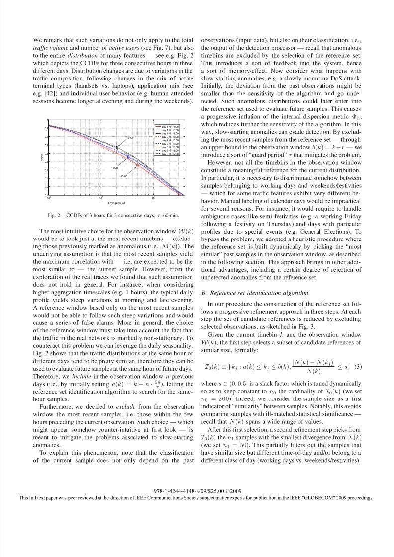
We remark that such variations do not only apply to the total

traffic volume and number of active users (see Fig. 7), but also

to the entire distribution of many features — see e.g. Fig. 2

which depicts the CCDFs for three consecutive hours in three

different days. Distribution changes are due to variations in the

traffic composition, following changes in the mix of active

terminal types (handsets vs. laptops), application mix (see

e.g. [42]) and individual user behavior (e.g. human-attended

sessions become longer at evening and during the weekends).

100

101

1020.1

0.2

0.3

0.4

0.5

0.6

0.7

0.8

0.9

1

# syn pkts_ul

C C D F

day 1 @ 15:00

day 1 @ 16:00

day 1 @ 17:00

day 2 @ 15:00

day 2 @ 16:00

day 2 @ 17:00

day 3 @ 15:00

day 3 @ 16:00

day 3 @ 17:00

17:00

16:00

15:00

Fig. 2. CCDFs of 3 hours for 3 consecutive days; τ =60-min.

The most intuitive choice for the observation window W (k)would be to look just at the most recent timebins — exclud-

ing those previously marked as anomalous (i.e. M(k)). The

underlying assumption is that the most recent samples yield

the maximum correlation with — i.e. are expected to be the

most similar to — the current sample. However, from the

exploration of the real traces we found that such assumption

does not hold in general. For instance, when considering

higher aggregation timescales (e.g. 1 hours), the typical dailyprofile yields steep variations at morning and late evening.

A reference window based only on the most recent samples

would not be able to follow such steep variations and would

cause a series of false alarms. More in general, the choice

of the reference window must take into account the fact that

the traffic in the real network is markedly non-stationary. To

counteract this problem we can leverage the daily seasonality.

Fig. 2 shows that the traffic distributions at the same hour of

different days tend to be pretty similar, therefore they can be

used to evaluate future samples at the same hour of future days.

Therefore, we include in the observation window n previous

days (i.e., by initially setting a(k) = k − n · 24τ

), letting the

reference set identification algorithm to search for the same-hour samples.

Furthermore, we decided to exclude from the observation

window the most recent samples, i.e. those within the few

hours preceding the current observation. Such choice — which

might appear somehow counter-intuitive at first look — is

meant to mitigate the problems associated to slow-starting

anomalies.

To explain this phenomenon, note that the classification

of the current sample does not only depend on the past

observations (input data), but also on their classification, i.e.,

the output of the detection processor — recall that anomalous

timebins are excluded by the selection of the reference set.

This introduces a sort of feedback into the system, hence

a sort of memory-effect. Now consider what happens with

slow-starting anomalies, e.g. a slowly mounting DoS attack.

Initially, the deviation from the past observations might be

smaller than the sensitivity of the algorithm and go unde-

tected. Such anomalous distributions could later enter into

the reference set used to evaluate future samples. This causes

a progressive inflation of the internal dispersion metric Φα,

which reduces further the sensitivity of the algorithm. In this

way, slow-starting anomalies can evade detection. By exclud-

ing the most recent samples from the reference set — through

an upper bound to the observation window b(k) = k −r — we

introduce a sort of “guard period” r that mitigates the problem.

However, not all the timebins in the observation window

constitute a meaningful reference for the current distribution.

In particular, it is necessary to discriminate somehow between

samples belonging to working days and weekends/festivities

— which for some traffic features exhibit very different be-havior. Manual labeling of calendar days would be impractical

for several reasons. For instance, it would require to handle

ambiguous cases like semi-festivities (e.g. a working Friday

following a festivity on Thursday) and days with particular

profiles due to special events (e.g. General Elections). To

bypass the problem, we adopted a heuristic procedure where

the reference set is built dynamically by picking the “most

similar” past samples in the observation window, as described

in the following section. This approach brings in other addi-

tional advantages, including a certain degree of rejection of

undetected anomalies from the reference set.

B. Reference set identification algorithm

In our procedure the construction of the reference set fol-

lows a progressive refinement approach in three steps. At each

step the set of candidate references is reduced by excluding

selected observations, as sketched in Fig. 3.

Given the current timebin k and the observation window

W (k), the first step selects a subset of candidate references of

similar size, formally:

I 0(k) ≡ {kj : a(k) ≤ kj ≤ b(k),|N (k) − N (kj)|

N (k)≤ s} (3)

where s ∈ (0, 0.5] is a slack factor which is tuned dynamically

so as to keep constant to n0 the cardinality of I 0(k) (we setn0 = 200). Indeed, we consider the sample size as a first

indicator of “similarity” between samples. Notably, this avoids

comparing samples with ill-matched statistical significance —

recall that N (k) spans a wide range of values.

After this first selection, a second refinement step picks from

I 0(k) the n1 samples with the smallest divergence from X (k)(we set n1 = 50). This partially filters out the samples that

have similar size but different time-of-day and/or belong to a

different class of day (working days vs. weekends/festivities).


978-1-4244-4148-8/09/$25.00 ©2009



0

0.2

0.4

0.6

0.8

1

# I M S I ( r e s c a l e d )

Sat Sun Mon Tue Wed Thu Fri Sat Sun

a(k) k b(k)

1)

2)

3)

N(k)+s

N(k)-s

0 (k)

1 (k)

(k)

I

I

I

Fig. 3. Logical sequence of the reference set identification algorithm.

The residual set I 1(k) might still contain heterogeneous

samples, e.g. due to clustered undetected anomalies or differ-

ent behavioral patterns with incidentally small divergence from

X (k). Furthermore, a tighter bundle of reference distributions

results in smaller internal dispersion Φα(k), which in turn

implies better sensitivity. Therefore, we resort to an heuristic

pruning procedure (third-step) to identify the dominant subset

of coherent distributions, as described in the following.

We adopt a graph-theoretic notation for convenience, and

introduce an undirected weighted complete graph G = (V , E )in which V ≡ I 1(k) and the weight of the edge (vi, vj) ∈ E is L(vi, vj). The pseudo-code of the algorithm is reported in

Fig. 4. The starting point is to separate the two most different

samples — i.e. those linked by the heaviest edge — obtaining

two single-element subsets A and B. The remaining edges are

then analyzed in descending order and the relative nodes are

put in either A or B, accordingly to the heuristic principle that

vertices linked by heavy edges are more likely to be different.

Of course this is true only in relative terms, but here the goal

is to identify the dominant group of similar distributions.

A ← ∅; B ← ∅;WHILE |A| + |B| < n1

(v1, v2) ← find heaviest edge(E ); E ← E \ {(v1, v2)};IF (v1 ∈ A) & (v2 /∈ B) & (v2 /∈ A) THEN B ← B ∪ {v2};ELSEIF (v2 ∈ A) & (v1 /∈ B) & (v1 /∈ A) THEN B ← B ∪ {v1};ELSEIF (v1 ∈ B) & (v2 /∈ A) & (v2 /∈ B ) THEN A ← A ∪ {v2};ELSEIF (v2 ∈ B) & (v1 /∈ A) & (v1 /∈ B ) THEN A ← A ∪ {v1};ELSE /*evaluate the two possible branches*/

A1 ← A ∪ {v1}; B1 ← B ∪ {v2};A2 ← A ∪ {v2}; B2 ← B ∪ {v1};IF mean weight(A1, B1) > mean weight(A2, B2) THEN

A ← A1; B ← B1;ELSE

A ← A2; B ← B2;

END IF

END IF

END WHILE

Fig. 4. Pseudo-code of the pruning heuristic (third step).

The function mean weight(A, B) is one of the possible

cost functions, and is defined as the mean weight of all edges

linking a vertex in A to a vertex in B. Hence, it is an indicator

of the dissimilarity between the two subsets, which we want

to be maximal. When the algorithm stops, the cardinality gap

between the two subsets is evaluated through the value of g =

abs|A|−|B||A|+|B|

. If g > 1 the subset with greater cardinality

is taken as the final I (k). Otherwise, no dominant subset is

elected and the whole V ≡ A ∪ B is taken, i.e. I (k) = I 1(k).

It is worth noting that, compared to classical clustering al-

gorithms, this procedure is less sensitive to the effect of strong

outliers, which is known to produce single-node clusters. As

mentioned above, the goal is not to achieve a hard clusteringbut rather a coarse pruning that increases the coherence of

final set by removing the most distant samples. The presented

heuristic was the result of extensive trials based on exploration

of a large dataset from the operational network.

VII. ANALYSIS OF REAL TRACES

Finally, we present some sample results from the application

of our algorithm to the real dataset. In Fig. 5 we report the

results for the sample feature “number of TCP SYN packets

in uplink” at 1-hour timescale for one week in August 2007

(the algorithm was initialized during the previous two weeks,

not shown in the figure). The uppermost green curve repre-

sents the internal dispersion bound Φα(k) (with α = 0.95)while red circles mark the alarms, i.e. the points where the

violation condition Γ(k) > Φα(k) was triggered. Note that

Φα(k) raises at night, when the number of active users N (k)decreases considerably, and therefore statistical fluctuations

become larger. From left to right, we see first a few isolated

alarms occurring at night time. These are due pre-planned

maintenance interventions in the network, which often involve

rebooting of some network element. Then we observe a cluster

of persistent alarms lasting an entire day (event “A”). This

was due to a temporary network problem, which was fixed

during the following night: a network element started suddenly

to misfunction, causing congestion on a network link. Some

mobile users affected by the problem reacted by re-startingslowed-down or stalled TCP connections, causing a change

in this feature distribution that was correctly reported as an

alarm. This is an excellent example of the type of events we

aim at detecting: with our tool deployed on-line, the network

staff would have been alarmed immediately.

Another cluster of persistent alarms is present later (event

“B”), lasting for 48 hours. The root cause was the worldwide

Skype outage August 20072. When a Skype client fails to

connect to other (super)nodes, it probes for other hosts and

port numbers in an attempt to bypass possible firewalls. Due

to the outage, the whole P2P network was temporary down,

so that all Skype clients active on mobile terminals reacted

simultaneously by entering into probing mode, causing a

change in this feature distribution (shown in Fig. 6) that

was correctly reported as an alarm. This is an illustrative

example of a macroscopic anomaly caused by an external

phenomenon, not local to the network domain. Although the

network operator in this case is not responsible for fixing

the problem, still it might be useful to be aware of what is

going on, for example to deal with customer complaints. We

2http://heartbeat.skype.com/2007/08/what happened on august 16.html


978-1-4244-4148-8/09/$25.00 ©2009



remark that such events, which are easily revealed by looking

at the entire distribution of SYN packets per-MS, might not

be clearly observable from the analysis of the total number

of SYN packets. The latter is shown in Fig. 7 (bottom graph)

along with the total number of active users N (k) (top).

A general issue with any statistical-based anomaly detection

scheme based on past data is that the detector needs to

be initialized with a “clean” anomaly-free data set. If the

initialization data contain anomalies, these should be manually

labeled and excluded from the reference set: in other words,

the initialization phase should be supervised by an expert. In

our case, the presence of spurious anomalies in the reference

set might widen the acceptability bound Φ(k)α, thus reducing

the detection power for a while after the initialization. How-

ever, the problem is mitigated by the fact that the algorithm

used to identify the reference set (ref. §VI-B) tends to prune

out distributions that are farther away from the main cluster.

Furthermore, since the reference set is updated at each step and

a maximum limit is set on the age of the reference observations

— a(k) in (eq. 3) — the effect of initial anomalies will

eventually fade out. Thanks to such features our algorithmcan tolerate impure initialization to a certain extent.

In some cases it is required to re-initialize the system. Fig.

8 shows the alarms generated on the feature “total number of

packets in uplink” in one such case. A link capacity upgrade

took place in the night before Thursday. Since then, the

user population reacted to higher available capacity generating

more traffic, so that the distribution of this feature changed

persistently. The sample distributions before/after the upgrade

are shown in the inset of Fig. 8. The change point was correctly

reported, but since the feature distribution never come back

to the previous behaviour, the system keeps generating alarms

indefinitely. In this case the human expert must reinitialize the

detection algorithm, forcing the system to “forget the past” bysetting a new observation window. In principle, it is possible

to implement automatic reinitialization scheme, e.g. based on

some threshold on the length of the alarm run. On the other

hand, only a human expert can decide whether the change is

a “legitimate” transition to a new equilibrium point, or rather

a long-lasting anomaly to be fixed.

VIII. CONCLUSIONS AND FUTURE RESEARCH

We have presented a novel scheme for traffic anomaly

detection in 3G mobile networks. Our approach is based on

the analysis of unidimensional distributions of certain fea-

tures across individual mobile users. Each feature is analysed

at different aggregation timescales, resulting in a grid of feature/timescale combinations which are processed indepen-

dently. We have observed that real anomalies tend to trigger

alarms across multiple features and timescales. For example,

the outage of a popular server or proxy would reduce the

rate of data packets in downlink, but would also temporarily

increase the rate of SYN packet in uplink due to client

retransmissions. Depending on its duration and intensity,

each anomaly tend to be visible across multiple neighboring

aggregation timescales. Therefore, alarm correlation (across

00:00 00:00

10−2

10−1

time [hh:mm]

D i v e r g e n c e m e a s u r e s

Sun Sun

Alarm

α %

mean

(1−α) %

A B

Fig. 5. Acceptance region Φα(k) (uppermost green line) and alarms (redcircles) over two weeks in August 2007, α = 0.95, τ = 60-min. The otherlines indicates the mean and 5-percentile of divergence values in I (k).

10 20 30 40 50 60 7010

−4

10−3

10−2

10−1

100

syn_pkts_ul (bin number)

C C D F

Normal

Skype outage

Fig. 6. Empirical Complementary Cumulative Distributions of feature“number of SYN packets in uplink”, τ = 60-min (bin number on x-axis).

features and timescales) appears to be a promising direction for

augmenting the accuracy of the detector. The idea is to tolerate

a higher probability of false alarm on individual detectors, and

then identify true alarms as clusters in the feature/timescale

space. This is a primary direction of our ongoing research,

together with the foreseen extension of the detector to work

with bivariate distributions (feature pairs).

An important lesson learned during the analysis of realtraces is that the interpretation of the reported alarms, i.e.

the diagnostic of its root cause, is often difficult and time-

consuming, and sometimes controversial. In many practical

cases the interpretation involves external information, techni-

cal (e.g., knowledge about recent network upgrades) and not.

For example, the introduction of a new tariff package, or the

release of a new popular client version, might cause sudden

00:00 00:00 00:00 00:00 00:00 00:00 00:00 00:00 00:00 00:00 00:00 00:00 00:00 00:00 00:000

0.2

0.4

0.6

0.8

1

time [hh:mm]

# s y n_

p k t s_

u l ( r e s c a l e d )

Tue Wed Thu Fri Sat Sun Mon Tue Wed Thu Fri Sat Sun Mon Tue

Tue Wed Thu Fri Sat Sun Mon Tue Wed Thu Fri Sat Sun Mon Tue

00:00 00:00 00:00 00:00 00:00 00:00 00:00 00:00 00:00 00:00 00:00 00:00 00:00 00:00 00:000

0.2

0.4

0.6

0.8

1

# M S ( r e s c a l e d )

A B

BA

Fig. 7. Number of active MS (top) and total number of SYN packets inuplink (bottom) for the same measurement interval of Fig. 5, τ = 60-min(absolute values are rescaled for non-disclosure policy).


978-1-4244-4148-8/09/$25.00 ©2009



00:00 00:00 00:00 00:00 00:00 00:00 00:00 00:00

10−3

10−2

10−1

time [hh:mm]

D i v e r g e n c e m e a s u r e s

Tue Wed Thu Fri Sat Sun Mon Tue

Alarmα %

mean

(1−α) %

Before the upgradeAfter the upgrade

Fig. 8. Acceptance region Φα(k) (uppermost green line) and alarms (redcircles) around a capacity upgrade, α = 0.95, τ = 60-min.

shift in the user behavior, hence in the traffic patterns and dis-

tributions. Therefore, while a detector can provide the means

to recognize the statistical syntax of anomalies, interpreting

their semantic will probably remain up to the human expert.

Since the interpretation of an alarm sometimes plays a role

in the detection of future alarms (e.g. for re-initialization), theinteraction with a human expert seems unavoidable in practice

also for the operation of the detector. We remark that such

limitation is not specific of our algorithm but applies in general

to any statistical-based anomaly detection scheme where past

data are used to evaluate current observations.

Our design choices were based on the exploration of large

sample datasets obtained from a real operational 3G mobile

network. It can be expected that the temporal traffic character-

istics that we have encountered — non-stationarities, seasonal-

ity, differences between working days vs. weekend/festivities,

long-term trend — are common ingredients to any large-scale

access network. Therefore, our change-detection algorithm

can be applied to any such network. Moreover, the proposedscheme can be applied to work in other contexts, inside

and outside the networking domain, as far as the data to be

analyzed have the form of distributional time-series.

REFERENCES

[1] H. Yang, et al., “Securing a wireless world,” IEEE Proceedings, vol. 94,no. 2, Feb. 2006.

[2] P. Traynor, P. McDaniel, and T. L. Porta, “On attack causality in internet-connected cellular networks,” in USENIX Security’07 , Aug. 2007.

[3] R. Kozma, et al., “Anomaly detection by neural network models andstatistical time series analysis,” in IEEE ICCN’94, Orlando, June 1994.

[4] M. Ostaszewski, F. Seredynski, and P. Bouvry, “A nonself space ap-proach to network anomaly detection,” in IPDPS, 20th Parallel and

Distributed Processing Symposium, IEEE, Ed., 25-29 April 2006.

[5] W. Chimphlee, et al., “Integrating genetic algorithms and fuzzy C-meansfor anomaly detection,” in IEEE Indicon’05, Chennai, India, Dec. 2005.

[6] S. T. Sarasamma, Q. A. Zhu, and J. Huff, “Hierarchical Kohonenen netfor anomaly detection in network security,” IEEE Trans. on Systems,man, and cybertnetics, vol. 35, no. 2, pp. 302–312, April 2005.

[7] A. Mitrokotsa and C. Douligeris, “Detecting denial of service attacksusing emergent self-organizing maps,” in 5th IEEE Int’l Symposium onSignal Processing and Information Technology, Dec. 2005, pp. 375–380.

[8] G.Prashanth, et al., “Using random forests for network-based anomalydetection,” in IEEE ICSCN’08, Chennai, India, 4-6 Jan. 2008, pp. 93–96.

[9] M. F. Pasha, R. Budiarto, and M. Syukur, “Connectionist model fordistributed adaptive network anomaly detection system,” in 4th Int’l

Conference on Machine Learning and Cybernetics, 18-21 Aug. 2005.

[10] T. Shon, et al., “A machine learning framework for network anomalydetection using SVM and GA,” in IEEE Workshop on Information

Assurance and Security, US Military Academy, West Point, NY, 2005.[11] Y. Li and L. Guo, “An efficient network anomaly detection scheme

based on TCM-KNN algorithm and data reduction mechanism,” in IEEE Workshop on Information Assurance and Security, US MilitaryAcademy, West Point, NY, 20-22 June 2007.

[12] P. Barford, J. Kline, D. Plonka, and A. Ron, “A signal analysis of network traffic anomalies,” in ACM SIGCOMM’02, 2002.

[13] M. Raimondo and N. Tajvidi, “A peaks over threshold model for change-

point detection by wavelets,” Statistica Sinica, vol. 14, 2004.[14] J. Brutlag, “Aberrant behavior detection in time series for network

monioting,” in Proc. USENIX 40th System Admin. Conf. LISA XIV , NewOrleans, LA, USA, Dec. 2000.

[15] H. Wang, D. Zhang, and K. Shin, “Detecting SYN flooding attacks,” IEEE Trans. on Information Theory, vol. 45, no. 3, April 1999.

[16] P. Lee, et al., “On the Detection of Signaling DoS Attacks on 3GWireless Networks,” in IEEE INFOCOM’07 , Anchorage, May 2007.

[17] G. Giorgi and C. Narduzzi, “Analysis of traffic flow measurements byrate-interval curves,” in Valuetools’06 , Pisa, Italy, 11-13, Oct. 2006.

[18] ——, “Detection of anomalous behaviors in networks from trafficmeasurements,” in IMTC’06 , Sorrento, Italy, 24-27, April 2006.

[19] H. Wang, D. Zhang, and K. Shin, “Statistical analysis of network trafficfor adaptive faults detection,” IEEE Trans. Neural Networks, vol. 16,no. 5, pp. 1053–1063, Sept. 2005.

[20] T. Ahmed, M. Coates, and A. Lakhina, “Multivariate online anomalydetection using kernel recursive least squares,” in IEEE INFOCOM ,

Anchorage, AK, USA, May 2007.[21] A. Lakhina, M. Crovella, and C. Diot, “Mining anomalies using traffic

feature,” in ACM SIGCOMM , Philadelphia, PA, USA, 22-26, Aug. 2005.[22] ——, “Diagnosing network-wide traffic anomalies,” in ACM SIG-

COMM , Portland, OR, USA, Aug. 2004.[23] A. Lakhina, et al., “Structural analysis of network traffic flows,” in ACM

SIGMETRICS, New York, NY, USA, June 2004.[24] A. Soule, K. Salamatian, and N. Taft, “Combining filtering and statistical

methods for anomaly detection,” in IMC ’05, Berkeley, CA, USA, 2005,pp. 331–344.

[25] M. Stoecklin, “Anomaly detection by finding feature distribution out-liers,” in ACM CONEXT , Lisboa, Portugal, 4-6 Dec. 2006.

[26] W. Lee and D. Xiang, “Information theoretic measures for anomalydetection,” Proc. Symposium on Security and Privacy, 2001, 130.

[27] Y. Gu, et al., “Detecting anomalies in network traffic using maximumentropy estimation,” in IMC , 2005, pp. 345–350.

[28] T. Dasu, et al., “An information-theoretic approach to detecting changes

in multi-dimensional data streams,” in INTERFACE’06 , Pasadena, CA,May 2006.

[29] J. Bannister, P. Mather, and S. Coope, Convergence Technologies for 3G Networks: IP, UMTS, EGPRS and ATM , Wiley, Ed., Dec. 2003.

[30] DARWIN homepage: http://userver.ftw.at/ ∼ricciato/darwin.[31] J. A. T. Thomas and T. M. Cover, Elements of Information Theory, J.

Wiley & Sons, Ed., 1991.[32] S. Ali and S. Silvey, “A general class of coefficients of divergence of

one distribution,” Journal of Royal Statistical Society, vol. 28, 1966.[33] I. Csiszar, “Information-type measures of difference of probability dis-

tributions and indirect observations,” Studia Sci. Math. Hungar., vol. 2,pp. 299–318, 1967.

[34] F. Liese and I. Vajda, Convex statistical distances. Teubner-Verlag, ’87.[35] A. Khayam and H. Radha, “Linear-complexity models for wireless

MAC-to-MAC channels,” ACM Wireless Networks, vol. 11, 2005.[36] X. Song, et al., “Statistical change detection for multi-dimensional data,”

in 13th ACM KDD ’07 . ACM, 2007, pp. 667–676.

[37] D. H. Johnson and S. Sinanovic, “Symmetrizing the Kullback-Leiblerdistance,” IEEE Transactions on Information Theory, March 2001.

[38] L. Paninski, “Estimation of entropy and mutual information,” NeuralComputation, vol. 15, pp. 1191–1253, 2003.

[39] ——, “Estimating entropy on m bins given fewer than m samples,” IEEE Transaction on Information Theory, vol. 50, no. 9, Sept. 2004.

[40] A. Papoulis, Probability, Random Variables and Stochastic Processes,3rd ed. McGraw Hill, 1991.

[41] R. E. Krichevsky and V. K. Trofimov, “The performance of universalencoding,” IEEE Transactions on Information Theory, no. 27, 1981.

[42] P. Svoboda, et al., “Composition of gprs/umts traffic : snapshots from alive network,” in IPS-MOME’06 , Salzburg,Austria, 27-28 Feb. 2006.

978-1-4244-4148-8/09/$25.00 ©2009

distribution-based anomaly detection in 3g mobile networks from theory to practice

Documents