Distribution Fields for Tracking

Laura Sevilla-Lara Erik Learned-MillerUniversity of Massachusetts Amherst{lsevilla, elm}@cs.umass.edu

Abstract

Visual tracking of general objects often relies on the as-sumption that gradient descent of the alignment functionwill reach the global optimum. A common technique tosmooth the objective function is to blur the image. However,blurring the image destroys image information, which cancause the target to be lost. To address this problem we intro-duce a method for building an image descriptor using distri-bution fields (DFs), a representation that allows smoothingthe objective function without destroying information aboutpixel values. We present experimental evidence on the su-periority of the width of the basin of attraction around theglobal optimum of DFs over other descriptors. DFs alsoallow the representation of uncertainty about the trackedobject. This helps in disregarding outliers during tracking(like occlusions or small misalignments) without modelingthem explicitly. Finally, this provides a convenient way toaggregate the observations of the object through time andmaintain an updated model. We present a simple trackingalgorithm that uses DFs and obtains state-of-the-art resultson standard benchmarks.

1. IntroductionIn this paper, we address the problem of searching for a

target in an image using gradient descent methods, i.e. localmethods of searching for a target match.

To implement tracking using local search, we mustchoose a representation for the target and the patch to whichwe are comparing it. There is a fundamental tension be-tween two conflicting goals when choosing such an imagerepresentation. On the one hand, we would like a matchingfunction whose global optimum represents the true positionof the target rather than a spurious match. We refer to thisproperty as the specificity of the descriptor.

On the other hand, we would like the optimization land-scape (of the matching function) to have few local minima.We refer to this as the landscape smoothness criterion.

There are many descriptors that exhibit one property butnot the other. For example, by blurring an image patch rep-

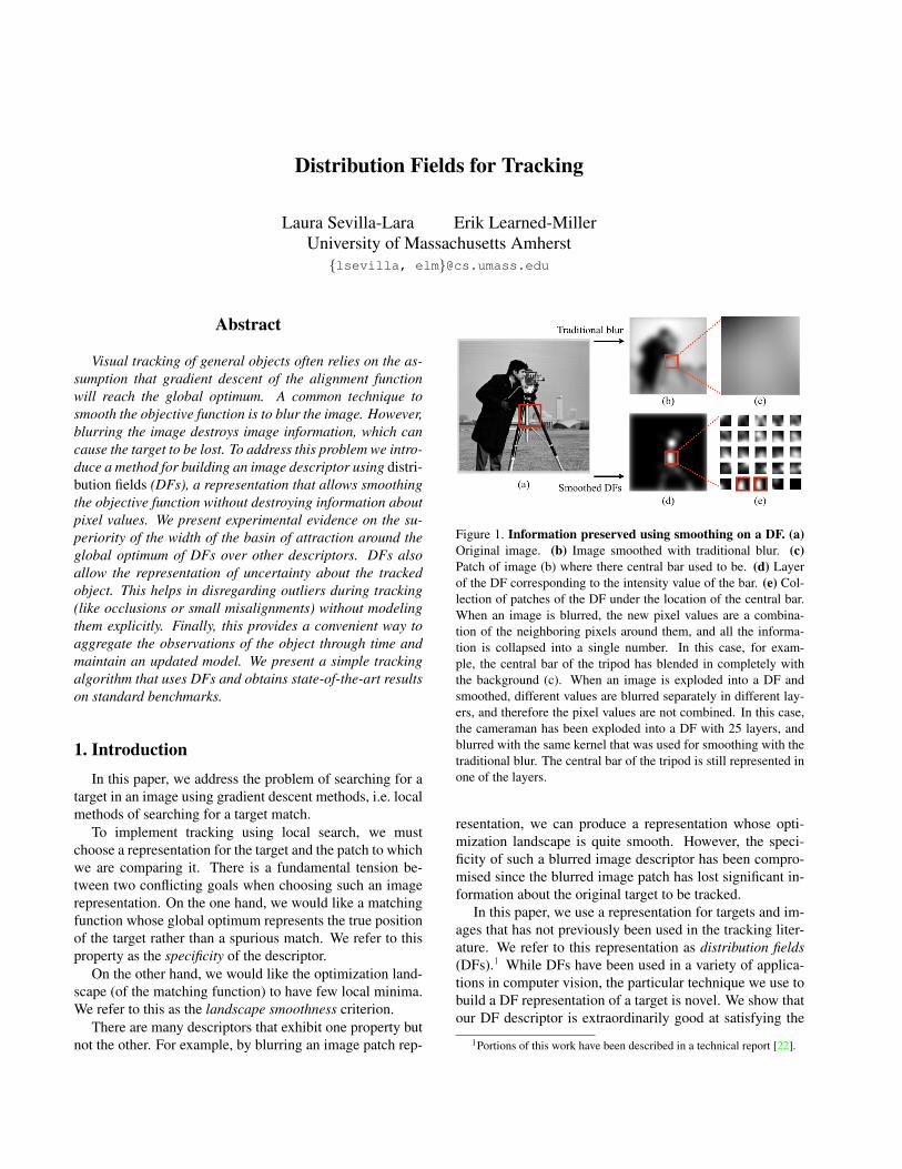
Figure 1. Information preserved using smoothing on a DF. (a)Original image. (b) Image smoothed with traditional blur. (c)Patch of image (b) where there central bar used to be. (d) Layerof the DF corresponding to the intensity value of the bar. (e) Col-lection of patches of the DF under the location of the central bar.When an image is blurred, the new pixel values are a combina-tion of the neighboring pixels around them, and all the informa-tion is collapsed into a single number. In this case, for exam-ple, the central bar of the tripod has blended in completely withthe background (c). When an image is exploded into a DF andsmoothed, different values are blurred separately in different lay-ers, and therefore the pixel values are not combined. In this case,the cameraman has been exploded into a DF with 25 layers, andblurred with the same kernel that was used for smoothing with thetraditional blur. The central bar of the tripod is still represented inone of the layers.

resentation, we can produce a representation whose opti-mization landscape is quite smooth. However, the speci-ficity of such a blurred image descriptor has been compro-mised since the blurred image patch has lost significant in-formation about the original target to be tracked.

In this paper, we use a representation for targets and im-ages that has not previously been used in the tracking liter-ature. We refer to this representation as distribution fields(DFs).1 While DFs have been used in a variety of applica-tions in computer vision, the particular technique we use tobuild a DF representation of a target is novel. We show thatour DF descriptor is extraordinarily good at satisfying the

1Portions of this work have been described in a technical report [22].

specificity and smooth landscape requirements of a goodtracking algorithm. We present several types of evidencesupporting this claim.

First, we show that our DF representation for trackinghas a wider basin of attraction around a target’s locationthan a large number of other descriptors that have been usedin the tracking literature (see Section 5). Second, we showthat a simple tracker built from this descriptor outperformsall other trackers on a standard tracking data set. Finally,we show that our tracker does not drift in a very long videosequence.

The paper is organized as follows. In Section 2 we de-scribe the previous work on descriptors for tracking. In Sec-tion 3 we define DFs and the operators over them. In Sec-tion 4 we describe the tracking algorithm. Section 5 showsexperimental evidence on the superiority on the basin of at-traction and tracking performance of DFs. Section 6 closeswith a discussion.

2. Previous workTracking algorithms have different aspects including

motion modeling, image representation and model update.The main focus of this work is the representation of the im-age using a descriptor that can overcome the challenges ofvisual tracking.

One common approach is to use a template to representthe object. This template can consist of the intensity val-ues, gradient information, or other features [3]. These tech-niques have limitations because they might be overly sen-sitive to the spatial structure of the object. This means thateven if the optimization reaches the global optimum, thismight not coincide with the correct position of the objectdue to changes in appearance. Robust metrics [18] allevi-ate this problem, but performance decays in long sequences[14]. DFs allow the representation of uncertainty in the de-scriptor, where small misalignments or occlusions can berepresented as “unlikely” events as opposed to “impossible”events, mitigating the oversensitivity to spatial structure.

Another problem with template-based methods is thatthe objective function might not be smooth enough to reachthe global optimum, as pointed out by Szeliski [24]. Often,the function is smoothed by blurring the image, for exampleusing a Gaussian pyramid [1]. Recently, it has been proventhat the Gaussian pyramid is not always the best choice forsmoothing the objective function [20], and alternative blurkernels have been derived [20] specifically for smoothingthe optimization landscape. Blurring the image has the un-desired effect of destroying information about the pixel val-ues. Depending on the size of the target, the levels of thepyramid and the characteristics of the background, the tar-get might disappear completely. In the DF framework, thelayered, or channel-by-channel, blurring technique allowssmoothing the objective function without the mix of infor-

mation that occurs in traditional blurring. This process isillustrated in Figure 1. The result is a smooth function witha wider basin of attraction around the object location thanother descriptors. Figure 5 shows an example in one of thebenchmark frames.

An alternative to building a template is using a histogramto describe the object [8, 6]. Histogram-based (also calledkernel-based) descriptors integrate information over a largepatch of the image. As a result they are not overly sensitiveto spatial structure and they provide a larger basin of attrac-tion. These methods have had a lot of success because theyare fast, simple, and invariant to many pose changes. Themain problem of kernel-based methods is the loss of spa-tial information that happens when building the histogram.This creates ambiguity in the optimization function [13] de-creasing the specificity of the descriptor. In order to resolvethese ambiguities, the size of the descriptor should be ex-panded. Recent efforts include some spatial information inthe descriptor by using multiple kernels [13], or multiplepatches [11]. These methods improve the performance ofthe single histogram descriptor, but require other mecha-nisms to decide the number and shape of the kernels. Fan etal. [12] propose a solution for the placement of the ker-nels, but a change in object appearance may make thesekernels unstable. Also, if the number of these kernels issmall, the tracking accuracy is more vulnerable to occlusionor abrupt motion. Other additions are higher order statistics[4] or temporal information [5], and using feature selection[7, 16, 26]. DFs capture the rich and robust informationcontained in a histogram while preserving the spatial struc-ture of the object by having a distribution at each pixel andcan be viewed as a soft combination of template-based andhistogram-based descriptors.

DFs are a generalization of many previous image repre-sentations used for different purposes. These previous de-scriptors can be viewed as special cases of DFs, and theyhave many of the desired properties listed above. To ourknowledge, only the general case of DFs together with theset of operators described in Section 3 presents all the prop-erties.

In background subtraction, Elgammal et al. [10], andStauffer and Grimson [23] use DFs for modeling the back-ground. A pixel is classified as background or foregrounddepending on the probability of belonging to the back-ground. These descriptors can adapt to changes in appear-ance and be robust to certain noise and illumination. How-ever, these descriptors do not spread information in space.

In object detection and recognition, descriptors likeHOG [9] and SIFT [17] use histograms of gradients. Thesecan be viewed as downsampled DFs with gradient as thefeature space. The large “support” of each histogram yieldsa smooth descriptor and a smooth objective function. How-ever, since the size of this “support” is fixed, the basin of

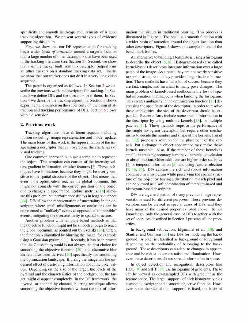
Figure 2. Left. DF after exploding the “cameraman” image. (Theoriginal image is shown superimposed on the DF for clarity.) Thenumber of brightness levels (or layers) has been quantized to 8.Right. The same DF after smoothing in the dimensions of theoriginal image.

attraction is much more limited.Another use of DFs was demonstrated by Learned-Miller

[15] in developing the congealing framework for joint im-age alignment. In this work, the likelihood of each imageis maximized with respect to the DF defined by the set ofimages. Congealing [15] has a large basin of attraction foralignment, since a collection of images can smooth the op-timization landscape.

Finally, the bilateral filter [25] introduced a way ofsmoothing an image such that both proximity in space andfeature value are taken into account to preserve image de-tail, which is similar to blurring using DFs.

3. Description of Distribution FieldsA DF is an array of probability distributions, one at each

pixel of the “field”. This distribution defines the probabilityof a pixel of taking each feature value. For example, if thefeature space is gray-scale intensity, then at each pixel thereis a probability distribution over the values 0-255.

Representation: A DF is represented as a matrix dwith(2 +N) dimensions, where the first two dimensions are thewidth and height of the image, and the other N dimensionsindex the feature space that we choose. For example, if thefeature space is intensity, then an image of sizem×n yieldsa 3D DF of sizem×n×b, where b is the number of intensityfeature values, or bins. For a higher dimensional featurespace, such as gradient, we can build a 2D distribution ateach pixel location, yielding a DF of four dimensions.

Construction: Exploding an image into a DF results ina Kronecker delta function at each pixel location. In par-ticular, exploding an image I into d with as many bins asfeatures values is defined by

d(i, j, k) ={

1 if I(i, j) == k0 otherwise,

where i and j index the row and column of the image, andk indexes the possible values of the pixel. We call the col-lection of bins at a fixed depth k a layer. This produces

a probability distribution at each pixel since the sum of thecomponents of each column is 1. The left side of Figure 2shows the results of computing this DF for the well-known“cameraman” image.

At this point, the DF representation contains exactly thesame information as the original representation, albeit in alarger representation. We now show how to “spread” theinformation in the image without destroying the brightnessvalues as occurs with traditional blurring.

The right side of Figure 2 shows a smoothed version ofthe DF on the left. The 3D DF has simply been convolvedwith a 2D Gaussian filter which spreads out in the x and ydimensions, but not in the feature dimension. That is, eachlayer k of the smoothed DF ds is computed as

ds(k) = d(k) ∗ hσs, (1)

where h is a 2D Gaussian kernel of standard deviation σs,and ∗ is the convolution operator.

Prior to convolution, we could interpret any value of 1in layer L of a DF to mean “there is a pixel of value L atthis location in the original image.” After convolution, thesemantics of the smoothed DF is, for any non-zero value ina layer L, “there is a pixel of value L somewhere near thislocation in the original image.” Thus, the convolution hasintroduced positional uncertainty into the representation. Acritical point is that no information has been lost about thevalue of pixels in the original image, only about their po-sition. This is because there has been no mixing of pixelvalues during the convolution process.

It is easy to show that if the convolution kernel in Equa-tion 1 is itself a probability distribution, then the smoothedds maintains the property that each column of pixels inte-grates to 1,2 and hence is still properly called a DF.

The previous discussion describes smoothing a DF in thex and y image dimensions. Smoothing can also take placein feature space. This allows the model to explain smallchanges due to subpixel motion, shadows, and changesin brightness. In a grayscale image, this smoothing is a1D Gaussian filter over the third dimension. Each of thecolumns of ds can be smoothed to produce dss as

dss(i, j) = ds(i, j) ∗ hσf, (2)

where hz is a 1D Gaussian kernel of standard deviation σf .In summary, exploding an image into a DF and smooth-

ing it can be viewed as introducing uncertainty about theobject appearance. A DF is then a compact representationof the image itself and a set of its “neighboring” images.These images are the result of transforming the originalimage with small changes in appearance and in location.

2This property breaks down at the boundaries of images. In order toavoid this problem, the missing information outside the boundaries is filledwith uniform distributions.

These are weighted according to the simple assumption thatthe most likely event is that the image will stay the same,and larger changes are less likely.

Comparison: The comparison between DFs that differ-ent images yield can be done with any distance function. Inthis paper we use the L1 distance between the two arrays d1

and d2 as:

L1(d1, d2) =∑i,j,k

|d1(i, j, k)− d2(i, j, k)|. (3)

Combination: Combining the information of severalDFs can also be useful. In tracking we combine the DFof initial model and the DFs of new observations using acomponent-wise convex combination of them, which alsoyields a DF:

dt+1(i, j, k) = λdt(i, j, k) + (1− λ)dt−1(i, j, k) (4)

By combining DFs of different instances of the same objectwe build a non-parametric data-driven model of the distri-bution at each pixel. This is useful for learning the statisticsof the appearance of the object during tracking.

4. Tracking algorithm detailsDFs can be used in a simple tracking algorithm. A model

of the target is created by exploding the image that containsthe target into a DF and smoothing it. Searching for the tar-get in a new frame consists of building a new DF by alsoexploding and smoothing the new frame, and following thedirection where the gradient of the L1 difference betweenthe DF of the model and the underlying part of the biggerDF representing the new frame descends. Once a local min-imum is reached, the model of the target is updated, usinga linear combination of the model and the new observation,as in Equation 4.

For better performance, we use a hierarchical approach.Instead of using a single DF to represent the target, we usea small set of DFs, where each of them is built using anincreasing value of the parameter σs, which regulates theamount of spatial blur. These DFs contain information atdifferent frequencies. At each frame, we use a coarse-to-fine strategy. The most smoothed DF is used to start thesearch, until it reaches a local minimum. This position isthe start for the search in the second DF.

The method for choosing the value of the parameters λand σf is using leave-one-out cross validation. The resultof picking σf separately for each video happens to coincidefor all of them to be σf = 10. This is also the case forλ = 0.95.

Parameter b corresponding to the number of bins waschosen, for speed, as the smallest power of two that doesnot hurt the performance of the videos. This is b = 16.

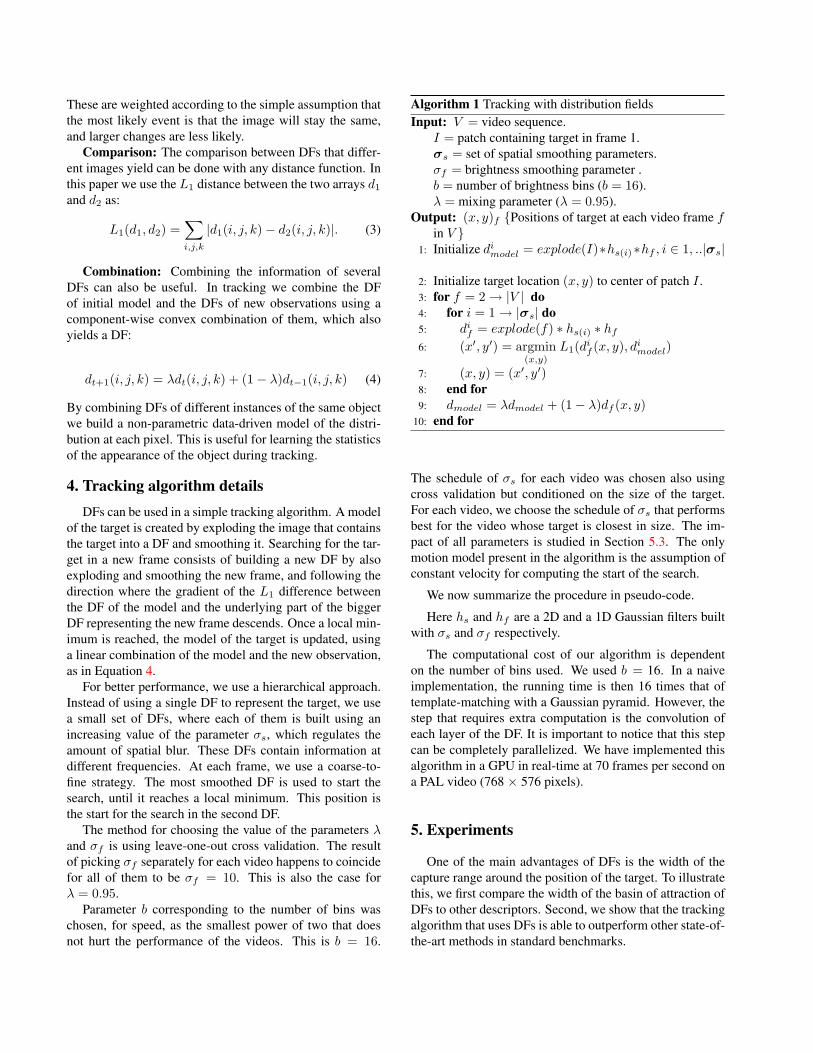
Algorithm 1 Tracking with distribution fieldsInput: V = video sequence.

I = patch containing target in frame 1.σs = set of spatial smoothing parameters.σf = brightness smoothing parameter .b = number of brightness bins (b = 16).λ = mixing parameter (λ = 0.95).

Output: (x, y)f {Positions of target at each video frame fin V }

1: Initialize dimodel = explode(I)∗hs(i)∗hf , i ∈ 1, ..|σs|

2: Initialize target location (x, y) to center of patch I .3: for f = 2→ |V | do4: for i = 1→ |σs| do5: dif = explode(f) ∗ hs(i) ∗ hf6: (x′, y′) = argmin

(x,y)

L1(dif (x, y), dimodel)

7: (x, y) = (x′, y′)8: end for9: dmodel = λdmodel + (1− λ)df (x, y)

10: end for

The schedule of σs for each video was chosen also usingcross validation but conditioned on the size of the target.For each video, we choose the schedule of σs that performsbest for the video whose target is closest in size. The im-pact of all parameters is studied in Section 5.3. The onlymotion model present in the algorithm is the assumption ofconstant velocity for computing the start of the search.

We now summarize the procedure in pseudo-code.

Here hs and hf are a 2D and a 1D Gaussian filters builtwith σs and σf respectively.

The computational cost of our algorithm is dependenton the number of bins used. We used b = 16. In a naiveimplementation, the running time is then 16 times that oftemplate-matching with a Gaussian pyramid. However, thestep that requires extra computation is the convolution ofeach layer of the DF. It is important to notice that this stepcan be completely parallelized. We have implemented thisalgorithm in a GPU in real-time at 70 frames per second ona PAL video (768 × 576 pixels).

5. Experiments

One of the main advantages of DFs is the width of thecapture range around the position of the target. To illustratethis, we first compare the width of the basin of attraction ofDFs to other descriptors. Second, we show that the trackingalgorithm that uses DFs is able to outperform other state-of-the-art methods in standard benchmarks.

5.1. Experiments on basin of attraction of Distribu-tion Fields

Here we evaluate the improvement in the basin of attrac-tion achieved by using DFs compared to other descriptors.

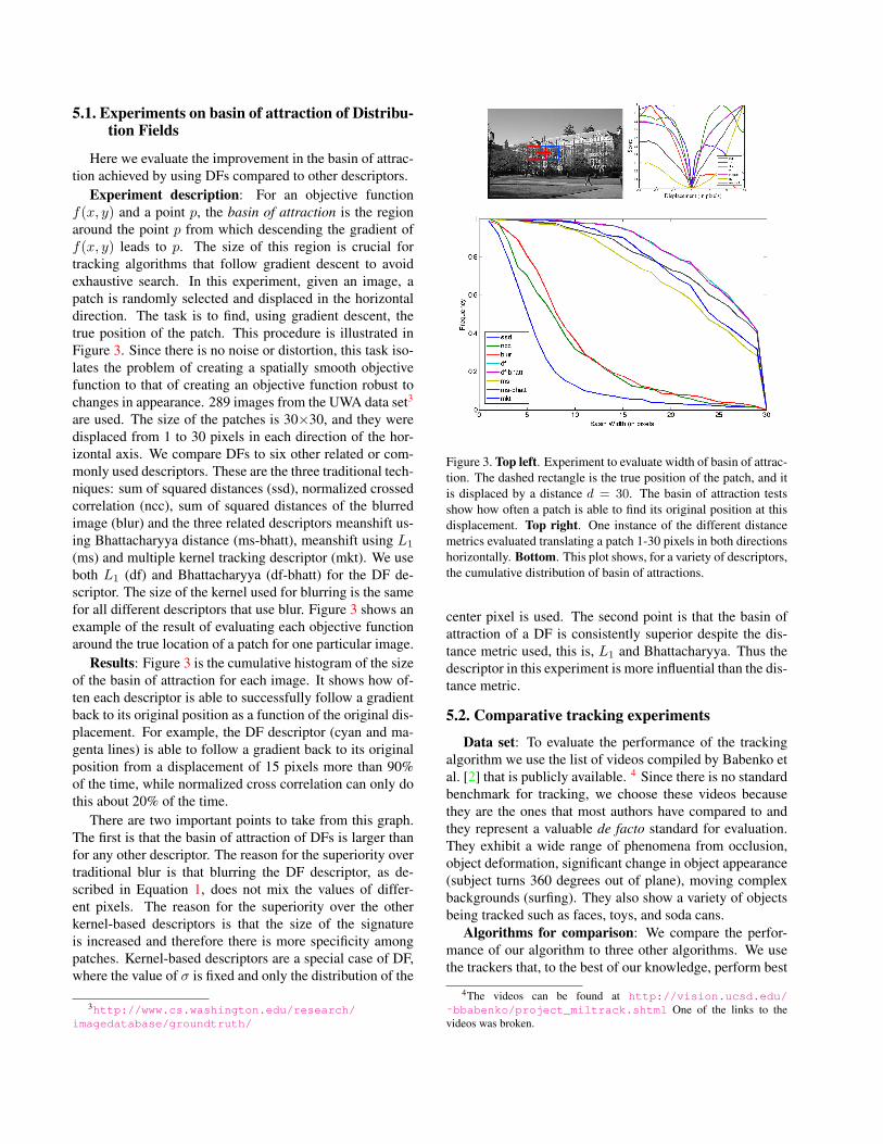
Experiment description: For an objective functionf(x, y) and a point p, the basin of attraction is the regionaround the point p from which descending the gradient off(x, y) leads to p. The size of this region is crucial fortracking algorithms that follow gradient descent to avoidexhaustive search. In this experiment, given an image, apatch is randomly selected and displaced in the horizontaldirection. The task is to find, using gradient descent, thetrue position of the patch. This procedure is illustrated inFigure 3. Since there is no noise or distortion, this task iso-lates the problem of creating a spatially smooth objectivefunction to that of creating an objective function robust tochanges in appearance. 289 images from the UWA data set3

are used. The size of the patches is 30×30, and they weredisplaced from 1 to 30 pixels in each direction of the hor-izontal axis. We compare DFs to six other related or com-monly used descriptors. These are the three traditional tech-niques: sum of squared distances (ssd), normalized crossedcorrelation (ncc), sum of squared distances of the blurredimage (blur) and the three related descriptors meanshift us-ing Bhattacharyya distance (ms-bhatt), meanshift using L1

(ms) and multiple kernel tracking descriptor (mkt). We useboth L1 (df) and Bhattacharyya (df-bhatt) for the DF de-scriptor. The size of the kernel used for blurring is the samefor all different descriptors that use blur. Figure 3 shows anexample of the result of evaluating each objective functionaround the true location of a patch for one particular image.

Results: Figure 3 is the cumulative histogram of the sizeof the basin of attraction for each image. It shows how of-ten each descriptor is able to successfully follow a gradientback to its original position as a function of the original dis-placement. For example, the DF descriptor (cyan and ma-genta lines) is able to follow a gradient back to its originalposition from a displacement of 15 pixels more than 90%of the time, while normalized cross correlation can only dothis about 20% of the time.

There are two important points to take from this graph.The first is that the basin of attraction of DFs is larger thanfor any other descriptor. The reason for the superiority overtraditional blur is that blurring the DF descriptor, as de-scribed in Equation 1, does not mix the values of differ-ent pixels. The reason for the superiority over the otherkernel-based descriptors is that the size of the signatureis increased and therefore there is more specificity amongpatches. Kernel-based descriptors are a special case of DF,where the value of σ is fixed and only the distribution of the

3http://www.cs.washington.edu/research/imagedatabase/groundtruth/

Figure 3. Top left. Experiment to evaluate width of basin of attrac-tion. The dashed rectangle is the true position of the patch, and itis displaced by a distance d = 30. The basin of attraction testsshow how often a patch is able to find its original position at thisdisplacement. Top right. One instance of the different distancemetrics evaluated translating a patch 1-30 pixels in both directionshorizontally. Bottom. This plot shows, for a variety of descriptors,the cumulative distribution of basin of attractions.

center pixel is used. The second point is that the basin ofattraction of a DF is consistently superior despite the dis-tance metric used, this is, L1 and Bhattacharyya. Thus thedescriptor in this experiment is more influential than the dis-tance metric.

5.2. Comparative tracking experiments

Data set: To evaluate the performance of the trackingalgorithm we use the list of videos compiled by Babenko etal. [2] that is publicly available. 4 Since there is no standardbenchmark for tracking, we choose these videos becausethey are the ones that most authors have compared to andthey represent a valuable de facto standard for evaluation.They exhibit a wide range of phenomena from occlusion,object deformation, significant change in object appearance(subject turns 360 degrees out of plane), moving complexbackgrounds (surfing). They also show a variety of objectsbeing tracked such as faces, toys, and soda cans.

Algorithms for comparison: We compare the perfor-mance of our algorithm to three other algorithms. We usethe trackers that, to the best of our knowledge, perform best

4The videos can be found at http://vision.ucsd.edu/

˜bbabenko/project_miltrack.shtml One of the links to thevideos was broken.

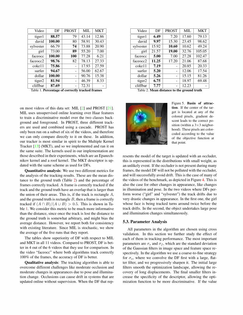
Video DF PROST MIL MKTtiger1 88.57 79 43.14 12.86david 100.00 80 58.91 30.43

sylvester 66.79 74 73.88 20.90girl 73.00 89 55.20 7.00

faceocc 100.00 100 77.28 6.21faceocc2 98.76 82 78.13 27.33

coke11 75.86 - 17.93 27.59surfer 94.67 - 56.00 62.67dollar 100.00 - 90.76 15.38tiger2 81.94 - 46.39 8.33

cliffbar 87.69 - 72.31 -Table 1. Percentage of correctly tracked frames

on most videos of this data set: MIL [2] and PROST [21].MIL uses unsupervised online learning over Haar featuresto train a discriminative model over the two classes back-ground and foreground. In PROST, three different track-ers are used and combined using a cascade. PROST hasonly been run on a subset of six of the videos, and thereforewe can only compare directly to it on these. In addition,our tracker is most similar in spirit to the Multiple KernelTracker [13] (MKT), and so we implemented and ran it onthe same suite. The kernels used in our implementation arethose described in their experiments, which are an Epanech-nikov kernel and a roof kernel. The MKT descriptor is up-dated with the same scheme as used for DFs.

Quantitative analysis: We use two different metrics forthe analysis of the tracking results. These are the mean dis-tance to the ground truth (Table 2) and the percentage offrames correctly tracked. A frame is correctly tracked if thetrack and the ground truth have an overlap that is larger thanthe union of their areas. This is, if the track is rectangle A,and the ground truth is rectangleB, then a frame is correctlytracked if (A ∩ B)/(A ∪ B) > 0.5. This is shown in Ta-ble 1. We consider this metric to be much more informativethan the distance, since once the track is lost the distance tothe ground truth is somewhat arbitrary, and might bias theaverage distance. However, we report both for consistencywith existing literature. Since MIL is stochastic, we showthe average of the five runs that they report.

The tables show superiority of DF with respect to MILand MKT in all 11 videos. Compared to PROST, DF is bet-ter in 4 out of the 6 videos that they use for comparison. Inthe video “faceocc” where both algorithms track correctly100% of the frames, the accuracy of DF is better.

Qualitative analysis: The tracking algorithm is able toovercome different challenges like moderate occlusion andmoderate changes in appearances due to pose and illumina-tion change. Occlusions can cause drift in systems that areupdated online without supervision. When the DF that rep-

Video DF PROST MIL MKTtiger1 6.49 7.20 17.60 79.13david 9.97 15.30 23.45 98.62

sylvester 15.92 10.60 10.62 49.24girl 21.57 19.00 32.76 105.05

faceocc 5.00 7.00 27.28 102.47faceocc2 11.25 17.20 21.06 87.68

coke11 7.19 - 20.85 20.33surfer 5.20 - 12.06 17.54dollar 5.26 - 15.15 81.26tiger2 6.75 - 18.97 69.48

cliffbar 7.77 - 12.23 -Table 2. Mean distance to the ground truth

Figure 5. Basin of attrac-tion. If the center of the tar-get is located at any of thecolored pixels, gradient de-scent leads to the correct po-sition (within a 3×3 neigbor-hood). These pixels are color-coded according to the valueof the objective function atthat point.

resents the model of the target is updated with an occluder,this is represented in the distributions with small weight, asan unlikely event. If the occluder is not present during manyframes, the model DF will not be polluted with the occluder,and will successfully avoid drift. This is the case of many ofthe videos of the benchmark, as depicted in Figure 4. This isalso the case for other changes in appearance, like changesin illumination and pose. In the two videos where DFs per-form worse (“girl” and “sylvester”) the track drifts due tovery drastic changes in appearance. In the first one, the girlwhose face is being tracked turns around twice before thetrack drifts. In the second, the object undertakes large poseand illumination changes simultaneously.

5.3. Parameter Analysis

All parameters in the algorithm are chosen using crossvalidation. In this section we further study the effect ofeach of them in tracking performance. The most importantparameters are σs and σf , which are the standard deviationof the Gaussian filters in image space and feature space re-spectively. In the algorithm we use a coarse-to-fine strategyfor σs, where we convolve the DF first with a large, flat-ter filter, and we progressively sharpen it. The initial largefilters smooth the optimization landscape, allowing the re-covery of long displacements. The final smaller filters in-crease the specificity of the descriptor, allowing the opti-mization function to be more discriminative. If the value

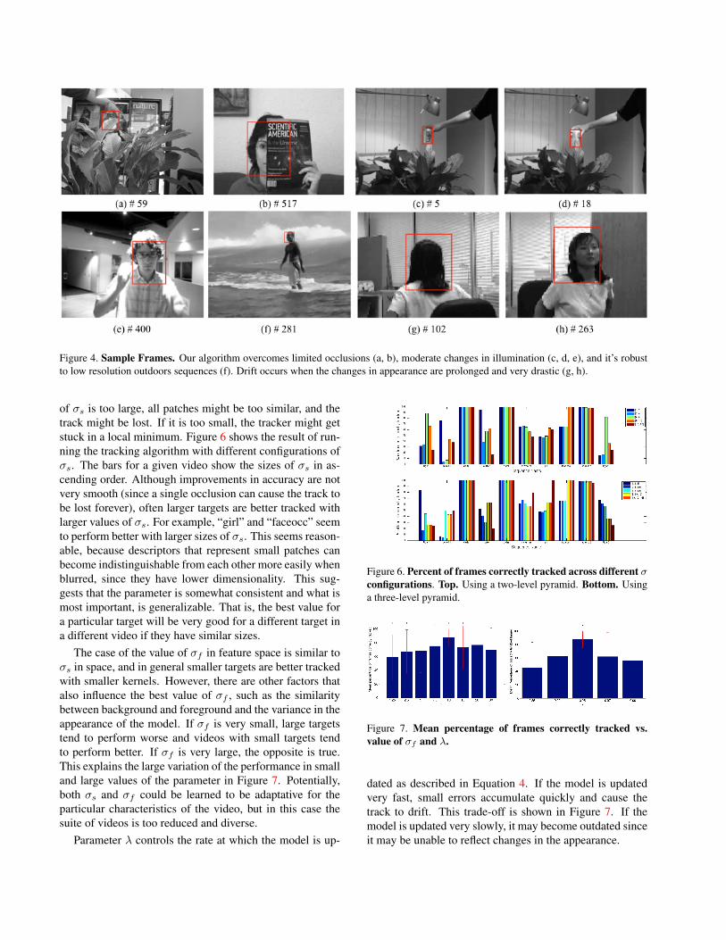
Figure 4. Sample Frames. Our algorithm overcomes limited occlusions (a, b), moderate changes in illumination (c, d, e), and it’s robustto low resolution outdoors sequences (f). Drift occurs when the changes in appearance are prolonged and very drastic (g, h).

of σs is too large, all patches might be too similar, and thetrack might be lost. If it is too small, the tracker might getstuck in a local minimum. Figure 6 shows the result of run-ning the tracking algorithm with different configurations ofσs. The bars for a given video show the sizes of σs in as-cending order. Although improvements in accuracy are notvery smooth (since a single occlusion can cause the track tobe lost forever), often larger targets are better tracked withlarger values of σs. For example, “girl” and “faceocc” seemto perform better with larger sizes of σs. This seems reason-able, because descriptors that represent small patches canbecome indistinguishable from each other more easily whenblurred, since they have lower dimensionality. This sug-gests that the parameter is somewhat consistent and what ismost important, is generalizable. That is, the best value fora particular target will be very good for a different target ina different video if they have similar sizes.

The case of the value of σf in feature space is similar toσs in space, and in general smaller targets are better trackedwith smaller kernels. However, there are other factors thatalso influence the best value of σf , such as the similaritybetween background and foreground and the variance in theappearance of the model. If σf is very small, large targetstend to perform worse and videos with small targets tendto perform better. If σf is very large, the opposite is true.This explains the large variation of the performance in smalland large values of the parameter in Figure 7. Potentially,both σs and σf could be learned to be adaptative for theparticular characteristics of the video, but in this case thesuite of videos is too reduced and diverse.

Parameter λ controls the rate at which the model is up-

Figure 6. Percent of frames correctly tracked across different σconfigurations. Top. Using a two-level pyramid. Bottom. Usinga three-level pyramid.

Figure 7. Mean percentage of frames correctly tracked vs.value of σf and λ.

dated as described in Equation 4. If the model is updatedvery fast, small errors accumulate quickly and cause thetrack to drift. This trade-off is shown in Figure 7. If themodel is updated very slowly, it may become outdated sinceit may be unable to reflect changes in the appearance.

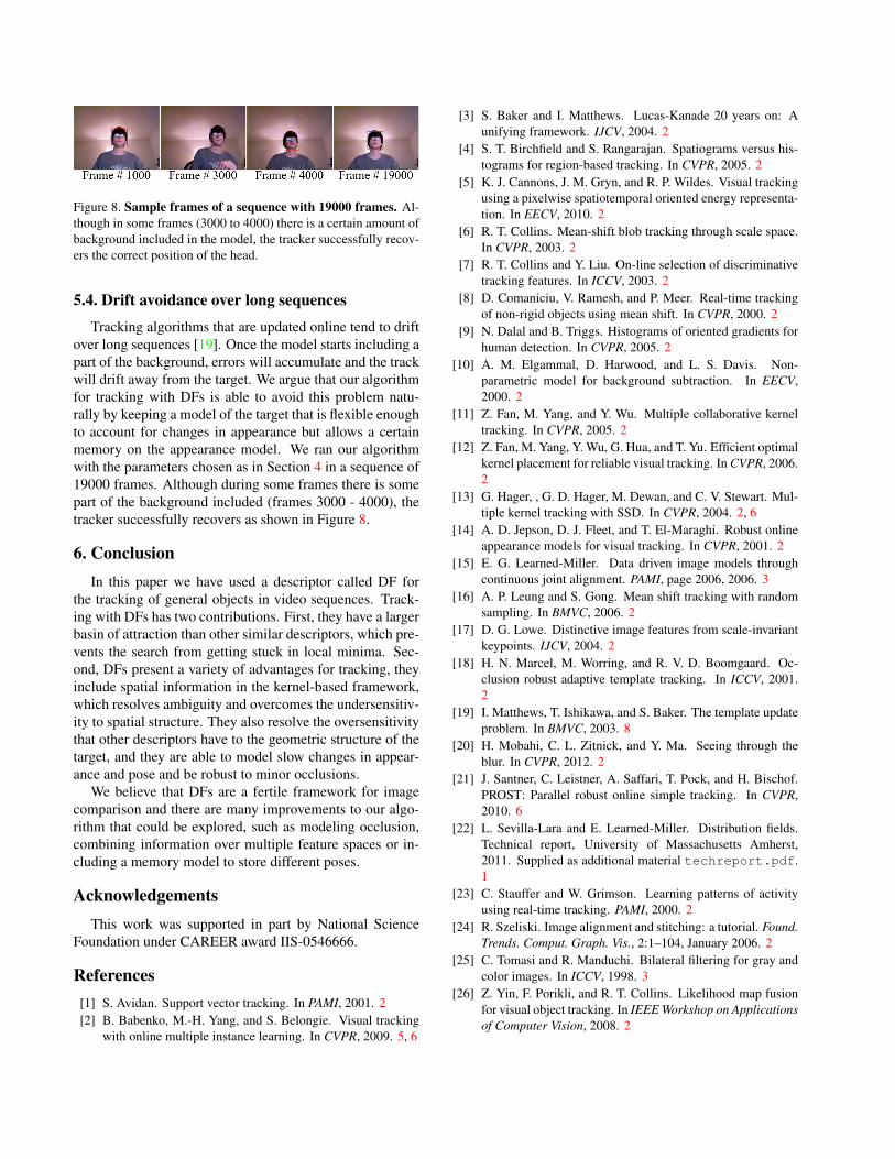
Figure 8. Sample frames of a sequence with 19000 frames. Al-though in some frames (3000 to 4000) there is a certain amount ofbackground included in the model, the tracker successfully recov-ers the correct position of the head.

5.4. Drift avoidance over long sequences

Tracking algorithms that are updated online tend to driftover long sequences [19]. Once the model starts including apart of the background, errors will accumulate and the trackwill drift away from the target. We argue that our algorithmfor tracking with DFs is able to avoid this problem natu-rally by keeping a model of the target that is flexible enoughto account for changes in appearance but allows a certainmemory on the appearance model. We ran our algorithmwith the parameters chosen as in Section 4 in a sequence of19000 frames. Although during some frames there is somepart of the background included (frames 3000 - 4000), thetracker successfully recovers as shown in Figure 8.

6. ConclusionIn this paper we have used a descriptor called DF for

the tracking of general objects in video sequences. Track-ing with DFs has two contributions. First, they have a largerbasin of attraction than other similar descriptors, which pre-vents the search from getting stuck in local minima. Sec-ond, DFs present a variety of advantages for tracking, theyinclude spatial information in the kernel-based framework,which resolves ambiguity and overcomes the undersensitiv-ity to spatial structure. They also resolve the oversensitivitythat other descriptors have to the geometric structure of thetarget, and they are able to model slow changes in appear-ance and pose and be robust to minor occlusions.

We believe that DFs are a fertile framework for imagecomparison and there are many improvements to our algo-rithm that could be explored, such as modeling occlusion,combining information over multiple feature spaces or in-cluding a memory model to store different poses.

AcknowledgementsThis work was supported in part by National Science

Foundation under CAREER award IIS-0546666.

References[1] S. Avidan. Support vector tracking. In PAMI, 2001. 2[2] B. Babenko, M.-H. Yang, and S. Belongie. Visual tracking

with online multiple instance learning. In CVPR, 2009. 5, 6

[3] S. Baker and I. Matthews. Lucas-Kanade 20 years on: Aunifying framework. IJCV, 2004. 2

[4] S. T. Birchfield and S. Rangarajan. Spatiograms versus his-tograms for region-based tracking. In CVPR, 2005. 2

[5] K. J. Cannons, J. M. Gryn, and R. P. Wildes. Visual trackingusing a pixelwise spatiotemporal oriented energy representa-tion. In EECV, 2010. 2

[6] R. T. Collins. Mean-shift blob tracking through scale space.In CVPR, 2003. 2

[7] R. T. Collins and Y. Liu. On-line selection of discriminativetracking features. In ICCV, 2003. 2

[8] D. Comaniciu, V. Ramesh, and P. Meer. Real-time trackingof non-rigid objects using mean shift. In CVPR, 2000. 2

[9] N. Dalal and B. Triggs. Histograms of oriented gradients forhuman detection. In CVPR, 2005. 2

[10] A. M. Elgammal, D. Harwood, and L. S. Davis. Non-parametric model for background subtraction. In EECV,2000. 2

[11] Z. Fan, M. Yang, and Y. Wu. Multiple collaborative kerneltracking. In CVPR, 2005. 2

[12] Z. Fan, M. Yang, Y. Wu, G. Hua, and T. Yu. Efficient optimalkernel placement for reliable visual tracking. In CVPR, 2006.2

[13] G. Hager, , G. D. Hager, M. Dewan, and C. V. Stewart. Mul-tiple kernel tracking with SSD. In CVPR, 2004. 2, 6

[14] A. D. Jepson, D. J. Fleet, and T. El-Maraghi. Robust onlineappearance models for visual tracking. In CVPR, 2001. 2

[15] E. G. Learned-Miller. Data driven image models throughcontinuous joint alignment. PAMI, page 2006, 2006. 3

[16] A. P. Leung and S. Gong. Mean shift tracking with randomsampling. In BMVC, 2006. 2

[17] D. G. Lowe. Distinctive image features from scale-invariantkeypoints. IJCV, 2004. 2

[18] H. N. Marcel, M. Worring, and R. V. D. Boomgaard. Oc-clusion robust adaptive template tracking. In ICCV, 2001.2

[19] I. Matthews, T. Ishikawa, and S. Baker. The template updateproblem. In BMVC, 2003. 8

[20] H. Mobahi, C. L. Zitnick, and Y. Ma. Seeing through theblur. In CVPR, 2012. 2

[21] J. Santner, C. Leistner, A. Saffari, T. Pock, and H. Bischof.PROST: Parallel robust online simple tracking. In CVPR,2010. 6

[22] L. Sevilla-Lara and E. Learned-Miller. Distribution fields.Technical report, University of Massachusetts Amherst,2011. Supplied as additional material techreport.pdf.1

[23] C. Stauffer and W. Grimson. Learning patterns of activityusing real-time tracking. PAMI, 2000. 2

[24] R. Szeliski. Image alignment and stitching: a tutorial. Found.Trends. Comput. Graph. Vis., 2:1–104, January 2006. 2

[25] C. Tomasi and R. Manduchi. Bilateral filtering for gray andcolor images. In ICCV, 1998. 3

[26] Z. Yin, F. Porikli, and R. T. Collins. Likelihood map fusionfor visual object tracking. In IEEE Workshop on Applicationsof Computer Vision, 2008. 2