diverse dimension decomposition for itemset spacesdisi.unitn.it/~themis/publications/kais12.pdf ·...

Under consideration for publication in Knowledge and InformationSystems

Diverse Dimension Decompositionfor Itemset Spaces

Mikalai Tsytsarau1, Francesco Bonchi2, Aristides Gionis2 and Themis Palpanas11University of Trento, Italy; 2Yahoo! Research Barcelona, Spain.

Abstract. We introduce the problem of diverse dimension decomposition in transac-tional databases, where a dimension is a set of mutually exclusive itemsets. The problemwe consider requires to find a decomposition of the itemset space into dimensions, whichare orthogonal to each other and which provide high coverage of the input database.The mining framework we propose can be interpreted as a dimensionality-reducingtransformation from the space of all items to the space of orthogonal dimensions.

Relying on information-theoretic concepts, we formulate the diverse dimension de-composition problem with a single objective function that simultaneously capturesconstraints on coverage, exclusivity and orthogonality. We show that our problem isNP-hard and we propose a greedy algorithm exploiting the well-known FP-tree datastructure. Our algorithm is equipped with strategies for pruning the search space deriv-ing directly from the objective function. We also prove a property that allows assessingthe level of informativeness for newly-added dimensions, thus allowing to define criteriafor terminating the decomposition.

We demonstrate the e!ectiveness of our solution by experimental evaluation on syn-thetic datasets with known dimension and three real-world datasets, flickr, del.icio.usand dblp. The problem we study is largely motivated by applications in the domain ofcollaborative tagging, however, the mining task we introduce in this paper is useful inother application domains as well.

Keywords: Diversity, transactional databases, dimension decomposition, informationtheory, collaborative tagging

1. Introduction

Collaborative content creation and annotation is one of the main activitiesand distinguishing features of the Web 2.0. Advances in social-media and user-

Received Dec 24, 2011Revised May 03, 2012Accepted May 13, 2012

2 M. Tsytsarau et al.

t1 {fish,art,film,portrait,tattoo,xpro,crossprocessed,nikon,skin,n80}t2 {sanfrancisco,black&white,building,art,stairway,fireescape,nikon}t3 {portrait,color,art,me,illustration,blood,adobephotoshop,canon}t4 {travel,brazil,plant,art,nature,color,strong,nikon,nikond70}t5 {sunset,art,museum,landscape,minneapolis,canon,powershotg3}t6 {sculpture,art,2004,festival,japan,culture,clay,a70,canon}t7 {portrait,art,painting,color,europe,sony,sonyericssonk750}t8 {black&white,art,film,photograph,street-photo,contax645}t9 {art,black&white,skin,hand,bodypainting,nikon,d70}t10 {red,woman,art,face,color,tear,canon,eos300d}t11 {art,3d,unfound,photositook,sony,cybershot}t12 {beautiful,woman,black&white,portrait,art}t13 {landscape,nature,sunrise,wallpaper,art}

Fig. 1. An example of transactional dataset, having three diverse dimensions(shown on the right). In this specific example from Flickr, each transaction cor-responds to a picture, and its associated tags. All pictures have in common thetag art.

generated content technologies have resulted in collecting extremely large vol-umes of user-annotated media; for instance photos (flickr), urls (del.icio.us),blogs (technorati), videos (youtube), songs (last.fm), scientific publications(bibsonomy and citeulike), and others. All these platforms provide users withthe capability of generating content and assigning tags, i.e., freely chosen key-words, to this content.

A repository of tagged resources can be seen as a transactional database,typical to the paradigm of frequent-itemset mining: transactions correspond toresources, and items correspond to tags. In this setting we are interested in study-ing the problem of discovering an item-space decomposition, which we define tobe a set of orthogonal dimensions with high coverage. A dimension in turn isdefined to be a set of itemsets that rarely co-occur in the database.

Example 1. Consider for instance a query on flickr for photos about art (i.e.,annotated with the tag art): the dataset D of such photos can look like the one inFigure 1. In this setting dimensions might be, for example, such sets of itemsetsas {{portrait},{landscape}} or {{canon},{nikon},{sony}}. Indeed, almost allphotos in the dataset contain at most one of the itemsets from each of the twodimensions.1

In particular, we are interested in discovering dimensions that represent di-verse concepts, such as “type of photo” or “camera brand”, and whose di!erentvalues almost partition the dataset. For instance, each dimension in Figure 1 canbe seen as a di!erent way of partitioning the transactions in D, and the threedimensions together can be considered as a diverse decomposition of the spaceof photos.

Extracting a set of diverse and orthogonal dimensions, that covers the var-ious aspects of the underlying dataset, can be seen as a problem of automaticfacet discovery, with plenty of applications in social-media and user-generatedcontent platforms. Whenever users label resources with tags, the automatic dis-covery of the relevant dimensions can improve user experience, e.g., facet-drivebrowsing and exploration, faceted search [11], tag recommendation [10], tag clus-tering [12, 13, 14, 15], and more. Similarly in recommender systems, whatever

1 While in this example each dimension is formed by singleton items, in general a dimensionis formed by itemsets of any size.

Diverse Dimension Decompositionfor Itemset Spaces 3

is the subject of the recommendation (movies, songs, books, etc.) structuringthe recommendation by means of automatically discovered facets (i.e., orthogo-nal dimensions) can improve the users experience and facilitate the discovery ofinteresting resources. In the scientific bibliography domains, discovering diverseand orthogonal dimensions can help highlighting the main trends in a scientificcommunity over a period of time.

Towards our goal, we adopt an information-theoretic perspective. While thereexist several studies applying joint entropy to the problem of identifying inter-esting or informative itemsets [1, 2, 4, 5, 6, 7], this body of work can not beapplied to the problem of diverse dimension decomposition, as explained next.Joint entropy is conventionally calculated as a sum of entropies over probabilities(frequencies) of set’s instances: H(X) = !

!p(Xi) log p(Xi), where instances

Xi " X are often represented as binary vectors, where bits at each position areindicating whether a particular item is present in the instance or not. In the fol-lowing example we demonstrate, that items in such sets are usually semanticallyunrelated:

Example 2. Consider a transposed view of the database from Figure 1, asshown in Table 1. Following the approaches that use joint entropy, we will getsets (templates) such as {color,nikon}, having the highest entropy (dark greylines), or {landscape,sony} as low-entropy sets (light grey lines).

We notice that high-entropy sets are characterized by more uniform appear-ance of their instantiations in the database (e.g., instances 01, 10 and 11 appearwith roughly the same frequency), while low-entropy sets accumulate supportaround the few most-frequent instances (in our example: 00), not necessarilyrepresenting mutually exclusive items forming the dimension (with instances001, 010, 100). Thus, using the existing interestingness measures does not solveour problem.

In this article, we propose an entropy measure that expresses both the or-thogonality among dimensions and the interestingness of dimensions. Moreover,we show that the proposed measure also captures constraints on exclusivity andcoverage. Based on this measure, we formulate diverse dimension decompositionas the problem of finding an optimal set of k dimensions, minimizing an objec-tive function that closely resembles the mutual information measure, except fora parameter !, which allows the analyst to trade-o! between information lossand orthogonality of the dimensions.

Our contributions are summarized as follows.– We introduce the novel problem of diverse dimension decomposition in trans-

actional databases, as an optimization problem. We characterize our objectivefunction and show that the selected dimensions explain well the underlyingdatabase.

– We prove a property that allows assessing the level of informativeness fornewly-added dimensions, thus allowing to define criteria for terminating thedecomposition.

– We show that our problem is NP-hard. We then propose a greedy algorithmexploiting the well-known FP-tree data structure [8]. Our algorithm prunesthe search space, based on properties of our objective function.

– We experiment with the proposed approach using two real-world large datasetsin the collaborative tagging domain, flickr and del.icio.us, and one dataset


Table 1. A transposed view of the dataset in Figure 1, showing most frequentitems taken from several dimensions.

item t1 t2 t3 t4 t5 t6 t7 t8 t9 t10 t11 t12 t13canon 0 0 1 0 1 1 0 0 0 1 0 0 0nikon 1 1 0 1 0 0 0 0 1 0 0 0 0sony 0 0 0 0 0 0 1 0 0 0 1 0 0color 0 0 1 1 0 0 1 0 0 1 0 0 0black&white 0 1 0 0 0 0 0 1 1 0 0 1 0landscape 0 0 0 0 1 0 0 0 0 0 0 0 1portrait 1 0 1 0 0 0 1 0 0 0 0 1 0

in the scientific bibliography domain (dblp) demonstrating the e!ectivenessand scalability of our solution.

– We introduce two methods, which generate synthetic datasets with distribu-tions of itemsets closely approximating the real data. Experiments on thesedatasets indicate that our method is able to withstand noise and reliably iden-tify dimensions even with small coverages.

– We evaluate, both theoretically and empirically, the ability of various itemsetsimilarity measures to facilitate the dimension decomposition. Moreover, weoutline several crucial properties for creating such measures.

The present article extends an earlier conference version [9] and has an up-dated formalism. In particular, itemset frequency is used instead of itemset sup-port count, and Theorem 2 is reformulated using ordered conditional entropies.The rest of the article is structured as follows. In the next section we discussrelated work and in Section 3 we formally define the problem of mining diversedimensions from a transactional dataset. In Section 4 we present our methods,while in Section 5 we report experimental assessment. Finally, we discuss futurework and conclude in Section 6.

2. Related work

We next survey the literature related to our work, dividing it into three groups:(i) methods that aim at extracting diverse content from web data, (ii) space-like representations of itemset databases, and (iii) entropy-based measures foritemset interestingness.

2.1. Diversity in information retrieval

Extracting a set of diverse dimensions, that covers the various aspects of theunderlying dataset, can be seen as a problem of facet discovery. Such a facet-discovery process has many applications in improving user experience, for in-stance, tag recommendation [10], search and exploration [11], tag clustering [12,13, 14, 15], and more. The work by Morik et al. [15], describing multi-objectivehierarchical termset clustering, represents an e!ective way of navigating tag-annotated resources. However, the hierarchical clusters produced in the abovework do not represent orthogonal dimensions, which is one of our main goals.

Web search is another domain in which finding an answer set with diversity is


important. Several studies have focused on the problem of search engines query-result diversification [16, 17, 18, 19], where the goal is to produce an answer setthat includes results relevant to di!erent aspects (facets) of the query.

2.2. Space-like representation of itemset databases

Traditionally, in association-rule mining, itemsets are represented as binary vec-tors in the space of items: each axis corresponds to an item, and binary coordinatevalues indicate whether each particular item is contained in the itemset. Thisrepresentation works well, if we are interested in finding association rules of theform {bread,milk} # {butter}, which capture itemset-level correlations indata. However, binary coordinates do not facilitate geometric decompositions ofthe item space (which can be interpreted by a human).

As a possible solution, Korn et al. [20] use real-valued coordinates, wherecoordinates can be interpreted as quantities of each item employed in the con-struction of rules. This framework allows to perform spectral decomposition ofthe item space (similar to SVD [21]), and to discover ratio rules, i.e., quantita-tive correlations among itemsets. An example of such rule is {1:bread,2:milk,5:butter}, which says that a typical ratio of bread, milk and butter within theitemsets is {1:2:5} , so we can predict missing values of di!erent items giventhese rules.

Alternatively, one can represent a database in the transposed space of trans-actions rather than items (like the one shown in Table 1). This is the main ideabehind the “geometrically inspired itemset mining” framework proposed by Ver-hein and Chawla [22]. Their proposal is a framework for frequent itemset mining,which can accept space transformations, such as SVD, subject to the constraintthat a measurement function should be able to be computed in the new space.For instance, in the case of SVD, each new axis represents a linear combinationof transactions, featuring the largest variance in data. However, such a transfor-mation is not very easily interpretable.

Our work is di!erent in that we propose a method for decomposing the spaceof items in a set of orthogonal dimensions that are readily interpretable. More-over, our problem formulation is based on information theory, and is capable ofidentifying dimensions in transactional databases in general, regardless whethertransactions have real values associated with items or not.

2.3. Entropy-based measures of itemset interestingness

Knobbe and Ho [1] define an information-theoretic measure for itemset inter-estingness, joint entropy, which is optimizing for uniform co-occurrence amongitems. In their terminology, a set is a template (or a collection of attributes takingbinary values), whose instances are itemsets. Entropy is calculated as a negativesum of logarithm-multiplied occurrence probabilities for observed instances. Thismeasure indicates how likely a randomly-chosen set instance is to appear in data.The same authors also introduced a notion of “pattern teams” [2], that can beseen as feature sets. They theoretically evaluate the e!ectiveness of di!erent fil-tering criteria for feature sets used in machine-learning classifiers, noticing thatthe measure of joint entropy does not satisfy the desirable properties that werequire from dimensions in this paper (i.e., mutual exclusivity, high coverage).


Table 2. Summary of notation used in this paper.I I ! I is an item X X " I is a pattern itemsetI I={I} is a set of all items !i !i ={Xi} is i-th dimensiont t " I is a transaction itemset ! ! = {!i} is a set of dimensionsD D={t} is a dataset of transactions I is a space of all possible itemsets: t ! I

Instead, the authors find that exclusive coverage (i.e., the sum of coverages mi-nus co-occurrences) is much more suitable as a measure optimizing for theseproperties.

Continuing the above line of research, Heikinheimo et al. define two relatedproblems, namely, mining high- and low-entropy sets [6]. Zhang and Masseglia [7]extend the method of Heikinheimo et al. to work on streaming data. They pro-pose to reduce the output size by removing similar sets according to criteriabased on mutual information [23]. A similar approach for counting subset fre-quencies was also used by Tatti [3] to define the significance (surprisingness)of itemsets, by comparing their Maximum-Entropy estimated frequency to theobserved one.

Finally, Tatti [4] and Mampaey et al. [5] propose to use joint entropy in anMDL optimization framework, aiming at compressing the database. Maximizingthe entropy ensures that all the pattern subsets are uniformly distributed, whilethe limit on pattern frequency (according to the exponential frequency decreaseassumption) facilitates the selection of frequent patterns.

Although these papers deal with itemset mining using joint entropy, their goalis di!erent from ours: they aim at extracting sets of items, which co-occur in thedatabase uniformly (when optimized for high entropy: same frequency for allsubset combinations) or sparsely (when optimized for low entropy: only certainsubsets are frequent). We discussed the di!erence between these approaches andour proposal earlier, in Example 2.

In contrast to the above methods, we formulate the entropy of a dimension asthe uncertainty of the dimension’s itemsets for each document, and use it as anindicator of quality for dimensions. Moreover, our goal is to find sets of itemsets(not items), which are not only mutually exclusive (within each dimension), butalso independent (across dimensions).

3. Notation, concepts, and problem statement

We are given a transactional dataset D, which is a multi-set of transactions t " I,where I is a ground set of items. An example of a transactional dataset is given inFigure 1. As usual we call itemset any set of items X " I, and we denote by D(X)its supporting set of transactions, i.e., D(X) = {t $ D | X " t}. Moreover wedenote by I the space of all possible itemsets on I. For the convenience, we arepresenting a short list of notation in Table 2.

In this paper we are studying the following problem. We are given an inte-ger k and the goal is to discover a collection of k dimensions, that decomposethe itemset space I. Moreover, we want each dimension to almost partition thedataset D; that is to say, we want (almost) all transactions t $ D to contain oneand only one of itemsets from the dimension.

Definition 1 (Dimension). Given an itemset space I, a dimension "i % I is a


collection of pairwise disjoint itemsets, i.e., "i = {X i0, ..., X

im}, such that for all

pairs of itemsets X ik, X i

l $ "i with l &= k it holds X ik ' X i

l = (.

As in decomposition methods in linear algebra, we want to decompose theitemset space in dimensions that can be though as “orthogonal.” While orthog-onality in linear algebra is a well-understood concept, when talking about theitemset space the concept of orthogonality is much less clear. Motivated by ourexample, we would like to argue that the dimension representing camera-brand{{canon},{nikon},{sony},...} is orthogonal to the dimension type-of-photograph{{portrait},{landscape},{street-photo},...}. The concept of orthogonalitycan thus be formulated as independence among the dimensions: the fact that aphotograph is tagged by nikon should not reveal any information about the typeof the photograph. That is, the likelihood of that photograph being portrait orlandscape should remain the same as it is non conditional on camera-brand.

To formalize the above intuition, we use the concept of mutual information.Given two random variables, X and Y , mutual information measures the infor-mation shared between them. For example, if X and Y are independent, thenknowing X does not give any information about Y and vice versa, so their mu-tual information is zero. In order to employ the definition of mutual information,we need to define precisely how our dimensions define a probability space, andwhat is the entropy of this probability space. We provide those definitions in thenext section.

In addition to finding orthogonal dimensions we also want to find “useful”dimensions, in the sense of being able to explain the dataset succinctly. Weexpress this intuition by the concept of coverage. In the previous example, thedimension camera-brand has high coverage because most of the photos have onetag among the itemsets {{canon},{nikon},...}. We are able to show that theconcept of coverage can also be formulated in an information theoretic manner.More importantly, we are able to combine both desiderata, high coverage andorthogonality, in one single objective function, achieving to simplify our problemformulation as well as the mining algorithm.

3.1. Entropy of dimensions

Our goal is to define the entropy H("i | D) of the dimension "i = {X i0, ..., X

im}

of the itemset space I, given the input dataset D. We first define the entropy ofthe dimension "i conditioned on a single transaction t of the dataset.

H("i | t) = !"

Xi!!i

P (X i | t) log P (X i | t)

The probabilities P (X i | t) express the uncertainty that the itemset X i ispresent in the transaction t, and are defined later in the section. Averaging overall transactions of the dataset D, we now define the entropy of the dimension "ias follows:

H("i | D) ="

t!DH("i | t)P (t),

where P (t) is the frequency of each transaction in the dataset. For instance, if


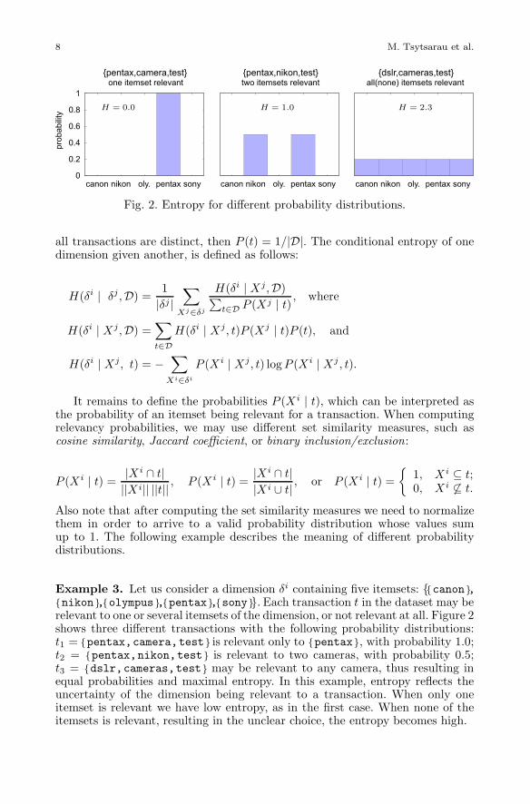
H = 0.0 H = 1.0 H = 2.3

Fig. 2. Entropy for di!erent probability distributions.

all transactions are distinct, then P (t) = 1/|D|. The conditional entropy of onedimension given another, is defined as follows:

H("i | "j ,D) =1|"j |

"

Xj!!j

H("i | Xj,D)!t!D P (Xj | t)

, where

H("i | Xj,D) ="

t!DH("i | Xj, t)P (Xj | t)P (t), and

H("i | Xj, t) = !"

Xi!!i

P (X i | Xj, t) log P (X i | Xj , t).

It remains to define the probabilities P (X i | t), which can be interpreted asthe probability of an itemset being relevant for a transaction. When computingrelevancy probabilities, we may use di!erent set similarity measures, such ascosine similarity, Jaccard coe!cient, or binary inclusion/exclusion:

P (X i | t) =|X i ' t|||X i|| ||t|| , P (X i | t) =

|X i ' t||X i ) t| , or P (X i | t) =

#1, X i " t;0, X i &" t.

Also note that after computing the set similarity measures we need to normalizethem in order to arrive to a valid probability distribution whose values sumup to 1. The following example describes the meaning of di!erent probabilitydistributions.

Example 3. Let us consider a dimension "i containing five itemsets: {{canon},{nikon},{olympus},{pentax},{sony}}. Each transaction t in the dataset may berelevant to one or several itemsets of the dimension, or not relevant at all. Figure 2shows three di!erent transactions with the following probability distributions:t1 = {pentax,camera,test} is relevant only to {pentax}, with probability 1.0;t2 = {pentax,nikon,test} is relevant to two cameras, with probability 0.5;t3 = {dslr,cameras,test} may be relevant to any camera, thus resulting inequal probabilities and maximal entropy. In this example, entropy reflects theuncertainty of the dimension being relevant to a transaction. When only oneitemset is relevant we have low entropy, as in the first case. When none of theitemsets is relevant, resulting in the unclear choice, the entropy becomes high.


3.2. Problem statement

As we mentioned before, the problem we consider is to discover k diverse di-mensions that explain well the input dataset. Let us denote by " = {"1, . . . , "k}such a set of k dimensions. Our objective function evaluates the goodness of thedimension set" in terms of entropy and diversity. We define these concepts next.

Definition 2 (Entropy of a dimension set). Given a set of dimensions" = {"1, . . . , "k}, its entropy is defined as the sum of entropies of its dimensions2

H(") ="

!i!!

H("i).

Definition 3 (Diversity of a dimension set). Given a set of dimensions" = {"1, . . . , "k}, its diversity is defined as the sum of conditional entropies overall pairs of dimensions

DIV (") ="

!i,!j!!

H("i | "j).

Central to our problem is the concept of mutual information, which we definehere for a pair of dimensions "i and "j .

Definition 4 (Mutual Information). The mutual information of two dimen-sions "i and "j is defined as follows

I("i; "j) = H("i) ! H("i | "j) = H("j) ! H("j | "i).

The mutual information of two dimensions is symmetric and is computed bytaking the di!erence between an entropy of the first dimension, H("i), and itsconditional entropy given another one, H("i | "j). The latter entropy expressesthe amount of information which one dimension contains about another, andwe want this amount to be low (this happens when the conditional entropy ofdimension "i remains large after we have identified dimension "j). In order toevaluate the goodness of the set of dimensions " we are summing the mutualinformation among all pairs of dimensions of the set ". We are now ready toformally define our problem.

Problem 1 (Diverse Dimension Decomposition). Given a dataset D, finda set of k dimensions " that minimize f("):

f(") =$H(") ! !

k ! 1DIV (")

%. (1)

In the above problem definition, we propose using an optimization functionf(") derived from mutual information.

Additionally, we introduce a parameter ! to control the e!ect of entropyand conditional entropy over the optimization criterion. One can notice that thevalue of ! = 1 corresponds to the case when the criterion is based precisely on

2 Throughout our paper we assume that all entropies are calculated with respect to the datasetD, omitting it in order to simplify the notation.


the pairwise sum of mutual informations, but we may pick any other positivereal value. This gives us the possibility to optimize either for information loss(when ! is small, e.g., ! = 0), orthogonality (when ! is large, e.g., ! = 1), orfor both (when ! takes an intermediate value).

Furthermore, we are able to show that by minimizing the objective func-tion (1) we are also ensuring that the resulting dimensions explain well theunderlying dataset. We first define the notion of coverage of a dimension.

Definition 5 (Coverage of a dimension). Coverage C(") of the dimension "on the dataset D is the fraction of transactions t in D, for which t ' X &= (, forsome itemset X $ ".

Definition 6 (Maximal co-occurrence of a dimension). We define themaximal co-occurrence R(") of the dimension " on the dataset D as the fractionof transactions t in D which contain all the itemsets from a subset {X} $ ", andnone of the other subsets of " are more frequent.

The following two lemmas are needed in our exposition that minimizing f(")ensures high coverage.

Lemma 1. If the value of the objective function is less than a threshold,f(") * #, then the entropy of the dimensions is also bounded:

H(") * #

1 ! ! .

Proof. For all pairs of dimensions "i and "j , we have that H("i | "j) * H("i),what implies that I("i; "j) + 0. In the case of a pairwise sum, DIV (") *(k ! 1)H("). Consequently, if [H(") ! !DIV (")/(k ! 1)] * # we have that[H(") ! !H(")] * #, or equivalently, H(")(1 ! !) * #.

The lemma implies that for values of ! + 1 the entropy becomes unbounded.In other words, when optimizing solely for orthogonality the quality (entropy)of dimensions may become uncontrollable as some of them can be added to acollection solely because of their high independence to others. This can happenfor dimensions that have negative contributions to f(") because of a high valueof the parameter !.

Property 1. For a dimension ", let s be the number of co-occurring itemsets ina transaction t, where 2 * s * |"|. Then, in the case of binary probabilities

P (X | t) =1s, and H(" | t) = !s

1s

log1s

= log s,

where in the case of no-coverage we have s = |"|, since all itemsets are equallyimprobable.

Lemma 2. Let " be a dimension with m itemsets, and consider the case thatthe probabilities P (X | t) take binary values. Then for the coverage C(") of thedimension " it should be

C(") + 1 ! H(")log m

.


Proof. Entropy takes its maximum value in the case that a transaction is notcovered by a dimension ". Applying Property 1, we have that max(H(" | t)) =log m. Therefore, the maximal ratio of not covered transactions would be lessthan H(") divided by the maximum entropy. Thus, 1 ! C(") * H(")/ logm,what proves the lemma.

Lemma 3. If probabilities P (X | t) are computed using binary similarities, thenmaximal co-occurrence R between any two itemsets in a dimension " should beless than its entropy per single transaction: R(") * H(").

Proof. Property 1 shows that the minimal entropy of single co-occurrence is equalto log 2. The maximal relative number of how many times the two itemsets mayco-occur would be H(") divided by the minimal entropy of single co-occurrence.Therefore, we have max(R(")) = H(")/ log 2 = H(").

We are now stating the theorem that small values of f(") imply high cover-age. The theorem is a direct consequence of Lemmas 1 and 2.

Theorem 1. Let " = {"1, . . . , "k} be a set of k dimensions and C(") be theirtotal coverage, defined as C(") =

!!i!! C("i). Finally, let m0 be the size of

the smallest dimension of ". If f(") * # then for the total coverage we have:

C(") + k ! #

(1 ! !) log m0.

Proof. According to Lemma 2, the sum of dimensions coverages is greater than:"

!i!!

C("i) + k !"

!i!!

H("i)log m

+ k !"

!i!!

H("i)log m0

Applying our notation and using Lemma 1, we have:

C(") + k ! H(")log m0

+ k ! #

(1 ! !) log m0!

We can use the above theorem to evaluate the quality of the dimensions, or tolimit the number of dimensions in the result, e.g., by conforming to the specifiedconstraint on the minimum coverage.

We next evaluate the dependency of f(") over the number of dimensions k.Suppose that we have a set of dimensions, and want to add another dimension.

Theorem 2. Adding a candidate dimension " will improve f(") as long asits average mutual information (across dimensions ") is less than the averageinformation of dimensions in " discounted by ( 1

" ! 1 + 1k )H(").

Proof. The di!erence d in the optimality value can then be written as follows:

d = H(") ! !k

DIV (" ) ") +!

k ! 1DIV (")

* H(") ! !k

[DIV (" ) ") ! DIV (")]

* H(") ! !k

"

!i!!

[H("|"i) + H("i|")]


We are interested in cases when this di!erence will be negative, correspondingto improving optimality:

H(") ! !k

"

!i!!

[H("|"i) + H("i|")] * 0, and since

H("|"i) + H("i|") = H(") + H("i) ! 2 · I("; "i), we have

H(") ! !k ! 1k

H(") ! !k

"

!i!!

H("i) +2!k

"

!i!!

I("; "i) * 0, equivalent to

1k

"

!i!!

I("; "i) * 12[1k

H(") ! (1!! 1 +

1k

)H(")] !

In other words, f(") will decrease when dimensions in " on average containless information about " than their average information discounted by H("). Aswe noted before, since I("; "i) is always greater than zero, smaller ! would re-quire addition of dimensions with smaller H(") to satisfy this condition, thusoptimizing for information loss. This property allows assessing the level of in-formativeness for newly-added dimensions, and defining criteria for terminatingthe decomposition.

4. Algorithm

We observe that Diverse Dimension Decomposition (Problem 1) is NP-hard, byreduction from the Set Partitioning problem, where we want to partition a setinto non-overlapping and non-empty parts that cover the entire set. This inherentcomplexity of the problem motivates us to seek for a heuristic algorithm. In therest of this section, we describe our solution based on a greedy strategy.

4.1. Algorithm overview

In order to solve the optimization problem of finding the optimal k dimensions,we propose identifying dimensions one-by-one. Our greedy strategy works as fol-lows. We start by constructing the first more prominent dimension, accordingto our objective function f("). The process begins with an empty single dimen-sion, and at each iteration we decide whether to add a new dimension, or growexisting itemsets, according to the strategies discussed below. The constructionof each dimension stops either if it is not possible to improve its score or if allitems have been partitioned. Then, we do the same for the remaining dimensionsiteratively, with the only di!erence that f(") now takes into account all the pre-viously identified dimensions, optimizing with respect to their orthogonality.

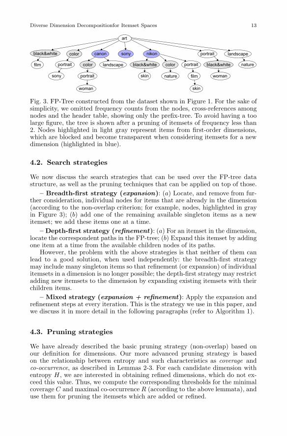
To store the data for our problem, we adopt a compressed database repre-sentation in the form of the well-known FP-Tree data structure [8]. In Figure 3,we show an example of such a tree, for the transactional dataset of Figure 1.This structure allows us to perform e#cient pruning based on the coverage,co-occurrence and non-overlap (partitioning) requirements, as explained next.


art

sony

sony nikon landscape

landscapeportrait portrait

portrait

portraitcanon

colorcolor

color

nature

nature

skin

skin film

film

woman

woman

black&white

black&white

black&white

Fig. 3. FP-Tree constructed from the dataset shown in Figure 1. For the sake ofsimplicity, we omitted frequency counts from the nodes, cross-references amongnodes and the header table, showing only the prefix-tree. To avoid having a toolarge figure, the tree is shown after a pruning of itemsets of frequency less than2. Nodes highlighted in light gray represent items from first-order dimensions,which are blocked and become transparent when considering itemsets for a newdimension (highlighted in blue).

4.2. Search strategies

We now discuss the search strategies that can be used over the FP-tree datastructure, as well as the pruning techniques that can be applied on top of those.

– Breadth-first strategy (expansion): (a) Locate, and remove from fur-ther consideration, individual nodes for items that are already in the dimension(according to the non-overlap criterion; for example, nodes, highlighted in grayin Figure 3); (b) add one of the remaining available singleton items as a newitemset; we add these items one at a time.

– Depth-first strategy (refinement): (a) For an itemset in the dimension,locate the correspondent paths in the FP-tree; (b) Expand this itemset by addingone item at a time from the available children nodes of its paths.

However, the problem with the above strategies is that neither of them canlead to a good solution, when used independently: the breadth-first strategymay include many singleton items so that refinement (or expansion) of individualitemsets in a dimension is no longer possible; the depth-first strategy may restrictadding new itemsets to the dimension by expanding existing itemsets with theirchildren items.

– Mixed strategy (expansion + refinement): Apply the expansion andrefinement steps at every iteration. This is the strategy we use in this paper, andwe discuss it in more detail in the following paragraphs (refer to Algorithm 1).

4.3. Pruning strategies

We have already described the basic pruning strategy (non-overlap) based onour definition for dimensions. Our more advanced pruning strategy is basedon the relationship between entropy and such characteristics as coverage andco-occurrence, as described in Lemmas 2-3. For each candidate dimension withentropy H , we are interested in obtaining refined dimensions, which do not ex-ceed this value. Thus, we compute the corresponding thresholds for the minimalcoverage C and maximal co-occurrence R (according to the above lemmata), anduse them for pruning the itemsets which are added or refined.


Algorithm 1: Mining Orthogonal DimensionsName : findNewDimensionInput : First-order dimensions " = {"k}, k < i,

Candidate dimensions candidates = {},FP-Tree, memoryBudget

Output: Optimal dimension "iout of order i1 repeat2 forall the dimension "i$candidates.unprocesseddo3 forall the itemset X i $ "i do4 forall the items I $ children(X i), I /$ "i," do5 if validItemset(X i ) {I} | "i) then6 //add one item to the current itemset7 "itemp = {"i | X i = X i ) {I}};

checkOptimality("itemp | ");candidates.temp.add("itemp);

8 end9 end

10 end11

refin

emen

tex

pans

ion

forall the items I $ I, I /$ "i," do12 if validItemset({I} | "i) then13 //add one more item as an itemset14 "itemp = "i ) {I};15 checkOptimality("itemp | "); candidates.temp.add("itemp);16 end17 end18 end19 //mark unprocessed as processed20 candidates += candidates.unprocessed;21 //newly generated become unprocessed22 candidates.unprocessed = candidates.temp;23 candidates.temp = {};24 //sort so that most optimal values are first25 candidates.sort();26 //remove candidates exceeding the allocated memory27 repeat28 candidates.remove(candidates.lastElement);29 until candidates.size > memoryBudget;30 until candidates.unprocessed.size > 0;31 return "iout = candidates.firstElement ;

4.4. Description of the algorithm

We formulate our optimization problem in a greedy fashion, relying on a mixedcandidate generation strategy and an iterative refinement of the candidate set.The complexity of this approach (almost) linearly depends on the size of thecandidate set (as seen in Figure 5), which we use as a parameter. Another inputof our algorithm is the FP-Tree, optionally containing only the most frequent


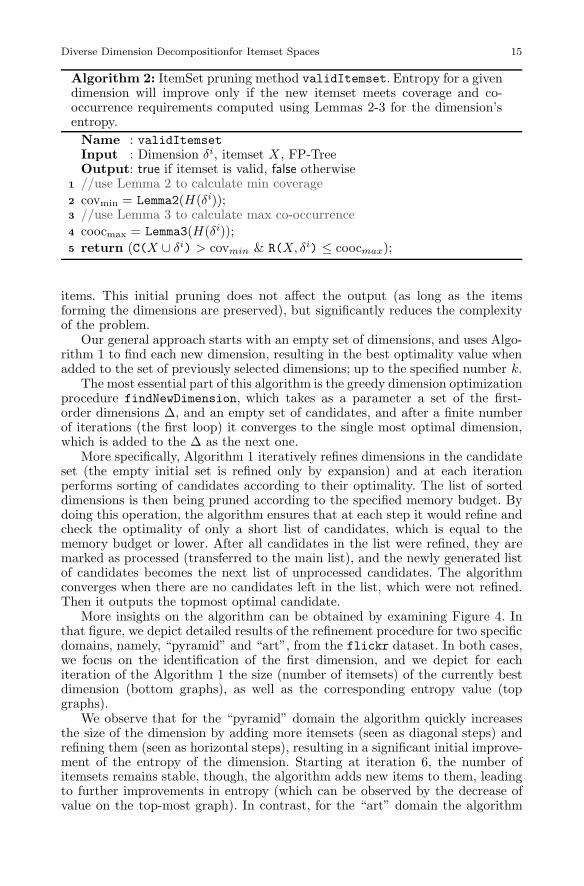
Algorithm 2: ItemSet pruning method validItemset. Entropy for a givendimension will improve only if the new itemset meets coverage and co-occurrence requirements computed using Lemmas 2-3 for the dimension’sentropy.Name : validItemsetInput : Dimension "i, itemset X , FP-TreeOutput: true if itemset is valid, false otherwise

1 //use Lemma 2 to calculate min coverage2 covmin = Lemma2(H("i));3 //use Lemma 3 to calculate max co-occurrence4 coocmax = Lemma3(H("i));5 return (C(X ) "i) > covmin & R(X, "i) * coocmax);

items. This initial pruning does not a!ect the output (as long as the itemsforming the dimensions are preserved), but significantly reduces the complexityof the problem.

Our general approach starts with an empty set of dimensions, and uses Algo-rithm 1 to find each new dimension, resulting in the best optimality value whenadded to the set of previously selected dimensions; up to the specified number k.

The most essential part of this algorithm is the greedy dimension optimizationprocedure findNewDimension, which takes as a parameter a set of the first-order dimensions ", and an empty set of candidates, and after a finite numberof iterations (the first loop) it converges to the single most optimal dimension,which is added to the " as the next one.

More specifically, Algorithm 1 iteratively refines dimensions in the candidateset (the empty initial set is refined only by expansion) and at each iterationperforms sorting of candidates according to their optimality. The list of sorteddimensions is then being pruned according to the specified memory budget. Bydoing this operation, the algorithm ensures that at each step it would refine andcheck the optimality of only a short list of candidates, which is equal to thememory budget or lower. After all candidates in the list were refined, they aremarked as processed (transferred to the main list), and the newly generated listof candidates becomes the next list of unprocessed candidates. The algorithmconverges when there are no candidates left in the list, which were not refined.Then it outputs the topmost optimal candidate.

More insights on the algorithm can be obtained by examining Figure 4. Inthat figure, we depict detailed results of the refinement procedure for two specificdomains, namely, “pyramid” and “art”, from the flickr dataset. In both cases,we focus on the identification of the first dimension, and we depict for eachiteration of the Algorithm 1 the size (number of itemsets) of the currently bestdimension (bottom graphs), as well as the corresponding entropy value (topgraphs).

We observe that for the “pyramid” domain the algorithm quickly increasesthe size of the dimension by adding more itemsets (seen as diagonal steps) andrefining them (seen as horizontal steps), resulting in a significant initial improve-ment of the entropy of the dimension. Starting at iteration 6, the number ofitemsets remains stable, though, the algorithm adds new items to them, leadingto further improvements in entropy (which can be observed by the decrease ofvalue on the top-most graph). In contrast, for the “art” domain the algorithm


0

0.1

0.2

0.3

0.4

0.5

0.6

0 2 4 6 8 10 12 14 16 18 0

1

2

3

4

5en

tropy

size

iteration

domain ’pyramid’

entropysize

0

0.1

0.2

0.3

0.4

0.5

0.6

0 2 4 6 8 10 12 14 16 18 0

2

4

6

8

10

12

14

entro

py

size

iteration

domain ’art’

entropysize

Fig. 4. Optimization statistics of the first dimension for “pyramid” and “art”(flickr).

starts with a dimension of good quality (low entropy), which after a single refine-ment (from iteration 1 to 2) stays on the top of the list of candidates till iteration9 (the value of entropy does not increase during this interval), while other candi-dates are being refined. Then, starting from the iteration 10, another candidate,refined to a better quality, takes its place and shows even better improvement inentropy. Finally, iterations converge and the best dimension is being identified.

We note that the final dimensions identified for the “pyramid” and “art”domains (after 17 and 15 iterations, respectively) are also the optimal singledimension decompositions for these domains.

5. Experimental evaluation

We evaluate our algorithm on both synthetic3 and real-world datasets. Evalua-tion of precision and performance is done in a controlled scenario, using large-scale synthetic datasets with artificially generated dimensions having itemsetdistribution similar to that of real datasets. We evaluate the time of decompo-sition and the quality of extracted dimensions depending on various noise andcoverage parameters and for several versions of our method. The observed re-sults convince that our method achieves good performance and is capable ofreconstructing dimensions even in most unfavorable conditions.

We provide additional evidence regarding the usability of our method by ap-plying it to two real-life datasets, containing tag-annotated resources, and onedataset, containing titles of scientific publications. The first dataset, extractedfrom flickr, a popular photos sharing website, contains 28 million tag-sets (ortransactions), obtained by taking annotations for all pictures that contain a spe-cific domain tag, for 34 di!erent domains. To remove noise, we allow only uniquetag-sets for each user id. The second dataset contains tag-sets from del.icio.us,a social bookmarking website. For this dataset, we select annotations for URLsstarting with specific domain names picked from Yahoo!Directory. Overall, thedel.icio.us dataset contains 1.7 million tag-sets over 150 domains. The num-ber of unique tags in each of the datasets is about half a million. The thirddataset, dblp4, is the largest collection of publications in the area of ComputerScience, containing more than 1.9 million titles organized by venue and year. Inour experiments, we used publications titles as sets of tags, removing stop-words,punctuation and duplicate words.

3 Synthetic datasets are available at http://disi.unitn.it/#tsytsarau/#content=Datasets4 DBLP database dump is publicly available at http://dblp.l3s.de/dblp++.php


A limited amount of additional cleaning is performed on all datasets by re-moving the domain term, numeric and navigational tags, as well as removingsome language variability, based on a custom-built dictionary. No sophisticatedpreprocessing is applied, so some of the discovered dimensions in our experimen-tal results still contain repetitions due to synonyms and misuse of tags.

We implement our algorithms in Java, and run the experiments under JavaJRE 1.6.13 on a machine with Intel Xeon 2.4 GHz processor, using a single coreand 1Gb of allocated memory.

5.1. Quantitative results on real datasets

In the first set of experiments, we report the execution time (Figure 5) and theentropy of the best solution found (Figure 6), as a function of the maximumnumber of candidates considered by our algorithm. We vary the number of itemsbetween 8 and 20, over the 150 domains of the del.icio.us dataset. In the graphs,we report the normalized values, averaged over all the 150 domains, as well as thestandard deviation for these values (for most of the points standard deviation istoo small and not visible). In order to make the results directly comparable toeach other, we first normalize each series using the minimum (maximum) valueof its regression line for the time (entropy) graph. Then, we compute the averagenormalized series, and its deviation.

In Figure 5, we report the averaged normalized execution times versus mem-ory budget. We observe, that an increase in number of items results to an increasein complexity. Overall, the algorithm scales linearly with respect to the memorybudget. When the number of items becomes large, the complexity is still deter-mined by the memory budget (remember, that at each iteration the number ofrefinements is proportional to the size of the candidate set).

In Figure 6, we observe that for a small number of items, an increase inmemory brings a considerably larger improvement in entropy, than for largernumbers of items. In the case of 8 items, the series drops until the entropy reachesits minimum for a maximum number of candidates of 32, which corresponds tothe optimal solution. For larger number of items, the same e!ect is observed fora higher setting of the maximum number of candidates.

5.2. Synthetic dataset generation

In order to evaluate various properties of our approach in a controlled environ-ment, we construct a synthetic dataset by generating itemsets for a number ofdimensions closely resembling dimensions found in real datasets. These dimen-sions contain two to five itemsets of sizes up to three items, and we require exactlytwo dimensions to be present in each dataset. We demonstrate an example of gen-erated dimensions in Table 3. Following the construction of dimensions, we usetwo di!erent ways of assuring their distribution in data, which are representedin Algorithms 3 and 4 and described as follows:Item-based generator (Algorithm 3) We calculate the frequency of single-ton items by applying Zipf’s law with a specified parameter z, f(Ik) , 1/kz.We chose this distribution because it is known to resemble word frequencies inreal-world datasets. Moreover, generating data from the Zipfian distribution al-lows to produce frequencies that are close to the uniform (when z is small), or


1 100

1 101

1 102

1 2 4 8 16 32 64 128

aver

age

norm

aliz

ed ti

me

max candidates number

20 items16 items12 items 8 items

Fig. 5. Time vs. memory budget.

1.00

1.01

1.02

1.03

1.04

1.05

1.06

1 2 4 8 16 32 64 128

aver

age

norm

aliz

ed e

ntro

py

max candidates number

20 items16 items12 items 8 items

Fig. 6. Entropy vs. memory budget.

the exponential (when z is large) distributions. Both of the extreme cases arechallenging for our problem, because with uniform frequencies non-dimensionalitems can occasionally form dimensions with a high coverage, and with exponen-tial frequencies higher-order dimensions have a very small coverage.

We then add a uniform noise of level $ to these frequencies, and harmonizethem for the items belonging to each of the dimension’s itemsets (to accountfor the observed rule that itemsets in dimensions usually have equally frequentitems; for example, both tags in {eiffeltower} usually appear together).Coverage-based generator (Algorithm 4) We randomly pick a coverage forthe itemsets of each dimension (i.e. the relative proportion of time each itemsetrepresents its dimension), assuring that this value is not smaller than 1/|"i|2. Toall the items allocated to dimensions are assigned frequencies of their respectingitemsets. To the rest of the items are assigned frequencies according to Zipf’sdistribution, scaled to half of the minimal frequency of allocated items. This stepis needed in order to assure that non-dimensional items would not occasionallyform any dimensions at the time of generating itemsets. As in the previousmethod, we add a uniform noise of level $ to these frequencies.Generating itemsets (Algorithm 5) For both of our methods, the itemsetsare generated by iteratively sampling the distribution of items with respect tothe specified dimensions. In this process, we use Gibbs sampling first to select adimension (independently from other dimensions) and then to select the itemsetrepresenting it (allowing for co-occurrence with a level of 0.5$). The rest of items,not covered by any dimension, are distributed with respect to their frequency.

In these experiments, we restrict the number of items to n = 16, which isequivalent to our minimum-support filtering on real datasets. Overall, we gener-ate 10 thousand itemsets for each set of parameters for the first dataset and onethousand for the second one, to ensure a smooth distribution according to ourmodel.

5.3. Experimental results on synthetic datasets

We assess the quality of the identified dimensions by comparing them to thedimensions used while generating the dataset. Our first similarity measure (usedin Figure 7) is based on Hamming distance d between two dimensions (repre-sented as binary vectors) divided by the total number of items: sim(";"0) =1 ! d(";"0)/n.

Since this measure is not able to distinguish incorrect positioning of items


Algorithm 3: Generating Item-based synthetic data.Input : Dimensions " = {"i}, number of itemsets n, noise level $, Zipf zOutput: Dataset D of itemsets

1 //generate frequencies for singleton items i, using Zipf’s law with noise2 f [Ik] = (1 + $%)/kz //random variable % is evenly distributed on [-0.5;0.5]3 //normalize and regularize frequencies4 f [Ik] = f [Ik]/

!f [Ik];

-X i $ "i from " and {Iik, Ii

l } $ X i : |f [Iik] ! f [Ii

l ]| * $;5 return D = GenerateItemsets(",n,$,frequencies);

Algorithm 4: Generating Coverage-based synthetic data.Input : Dimensions " = {"i}, number of itemsets n, noise level $,

Zipf z, coverage C.Output: Dataset D of itemsets

1 //randomly generate frequencies for dimension itemsets2 f [X i

j] = 1/|"i| + (1 ! 1/|"i|)%1 //%1 is uniformly distributed on [0;1]3 f [X i

j] = f [X ij]/f ["i]; //normalize frequencies within each dimension

4 //add noise to frequencies5 forall the items Ik do6 if Ik $ X i

j then f [Ik] = f [X ij ];

7 else f [Ik] = 0.5 C min(f [X ij])/kz;

8 f [Ik] = f [Ik](1 + $%2); //%2 is uniformly distributed on [-0.5;0.5]9 end

10 return D = GenerateItemsets(",n,$,frequencies);

Algorithm 5: Generating itemsets GenerateItemsets(", n, $, frequencies).1 forall the transaction t $ D, 1..n do2 while |t| = 0 do3 forall the dimension "i $ " do4 //sample the dimension using uniform %3 and %45 if %3 < C then6 repeat sample X i with co-occurrence level at 0.5$7 //sample the itemset using Gibbs method8 X i = GibbsSampling("i, f [X i]); t = t ) X i;9 until %4 > 0.5$;

10 end11 end12 forall the non-allocated items Ik do13 //sample according to f [Ik] using Gibbs method14 Ik = GibbsSampling(I, f [Ik]); t = t ) Ik;15 end16 end17 end18 return D;


Table 3. An example of dimensions used by Algorithms 3 and 4!1 {{0}, {1}, {2}, {3, 4}}, {{5, 6}, {7}}!2 {{0}, {1, 2}, {3, 4}}, {{5, 6}, {7}}!3 {{0}, {1}, {2}}, {{5}, {6}}!4 {{0}, {2}, {3}}, {{4, 5}, {6}, {7}}!5 {{0}, {1}, {2}, {3}, {4}}, {{5}, {6}, {7}}!6 {{0, 1}, {2}, {3}, {4}}, {{5}, {7}}!7 {{0}, {1}, {2, 3}, {4}}, {{6}, {7}}!8 {{0}, {1, 2}, {3, 4}}, {{5}, {6, 7}}!9 {{0}, {1}, {3}}, {{2}, {4}}!10 {{0}, {2}, {4}}, {{1}, {3, 5}}

0.6

0.7

0.8

0.9

1.0

0 0.05 0.1 0.15 0.2

aver

age

sim

ilarit

y

noise level

zipf 1.2 zipf 0.8 zipf 0.4

Fig. 7. Similarity to optimaldimensions versus noise.

-10-8-6-4-2 0 2 4 6

1 2 3 4 5 6

aver

age

norm

aliz

ed o

ptim

ality

number of dimensions

alpha 0.25alpha 0.50alpha 0.75

Fig. 8. f(") dependency onthe number of dimensions.

within identified dimensions, in the subsequent experiments we use its more elab-orate derivative, i.e., averaging similarities between the corresponding itemsetswithin each dimension. To achieve this, we first map dimensions to each otheraccording to maximal sim("i;"j) between them, and then average similaritiesbetween itemsets using the same mapping method.

These measures take values in the range [0, 1], with higher values indicatingstronger similarity: a value of 1 means that the algorithm correctly identifiedthe planted dimensions. We note that these measures do not account for thevarying significance of items, which is not favoring our approach, since includinglow-support items in the dimensions represents a challenge, even without theadditional noise.

The evaluation of quality against noise for di!erent parameters z is shown inFigure 7. In gray lines we plot the 0.95 confidence intervals for average values.

We can see that regardless of the noise added, our method is able to recon-struct almost perfectly the optimal dimensions for a wide range of distributions.As expected, the similarity between the identified and the optimal dimensionsdecreases on average with growing noise, and is significantly lower for smallerparameters z (more uniform items distribution).

In Figure 8 we evaluate the monotonicity of f(") over the number of dimen-sions k, for di!erent values of ! parameter. It is clearly visible that for smallvalues of ! optimality gets higher (worse), while for large values every new di-mension improves optimality (albeit, not the quality of extracted dimensions).For our experiments we chose ! = 0.5, since it provides a good balance betweenorthogonality and interestingness, and allows to rely on Theorem 2 (controllingthe decomposition) for a wide range of data distributions.


Table 4. Top dimensions for di!erent domains in flickr and del.icio.us.!i collection of itemsets for !i (flickr)

domain “jaguar”1 {automobile}, {zoo}2 {etype}, {auto}

domain “ei!el tower”1 {paris france europe tower}, {lasvegas}2 {night seine}, {holiday travel}3 {architecture}

domain “pyramid”1 {egypt giza cairo sphinx}, {louvre paris

museum glass}, {mexico maya ruins},{sanfrancisco transamerica}

2 {france sky}, {travel teotihuacan}3 {architecture night}, {chichenitza}

domain “hollywood”1 {losangeles california sign},

{star film actor}2 {us universalstudios}, {hollywoodboulevard

night}3 {theatre party sunset}, {canon street}

domain “art”1 {painting drawing}, {graffiti streetart},

{sculpture museum}, {newyork}, {color},{photo}, {street}

domain “spain”1 {barcelona catalonia}, {madrid europe},

{andalusia granada}, {seville},{valencia}, {holiday travel}

2 {architecture}

!i collection of itemsets for !i (del.icio.us)domain “nytimes.com”

1 {news politics}, {food health}, {science},{article}, {business}, {technology}

domain “dpreview.com”1 {photo camera review}, {dslr}2 {digital}3 {shopping}

domain “lifehacker.com”1 {howto lifehacks tips},{software windows

tools freeware}2 {firefox internet}, {linux utilities},

{email extensions}, {mp3 download},{organization toread}, {photography}

domain “apple.com”1 {mac osx software},{ipod itunes

music},{video quicktime},{movies trailers},{iphone},{podcastpodcasting},{technology}

2 {macosx howto}domain “microsoft.com”

1 {windows software tools},{.net programming}2 {security xp}3 {utilities}

domain “ixbt.com”1 {hardware software news computers russian},

{photo photography}2 {article}3 {reviews}

5.4. Qualitative results on real datasets

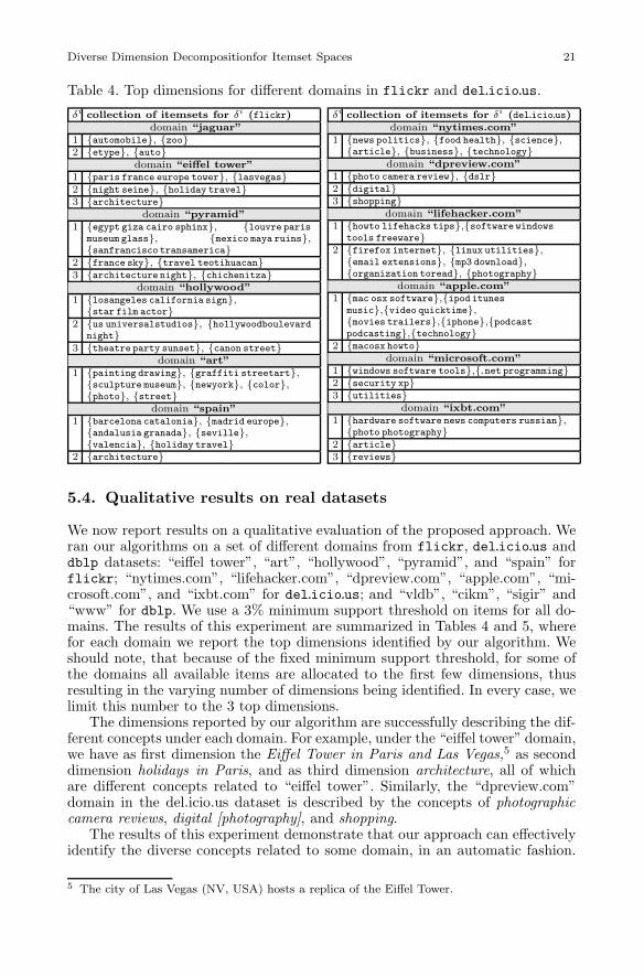
We now report results on a qualitative evaluation of the proposed approach. Weran our algorithms on a set of di!erent domains from flickr, del.icio.us anddblp datasets: “ei!el tower”, “art”, “hollywood”, “pyramid”, and “spain” forflickr; “nytimes.com”, “lifehacker.com”, “dpreview.com”, “apple.com”, “mi-crosoft.com”, and “ixbt.com” for del.icio.us; and “vldb”, “cikm”, “sigir” and“www” for dblp. We use a 3% minimum support threshold on items for all do-mains. The results of this experiment are summarized in Tables 4 and 5, wherefor each domain we report the top dimensions identified by our algorithm. Weshould note, that because of the fixed minimum support threshold, for some ofthe domains all available items are allocated to the first few dimensions, thusresulting in the varying number of dimensions being identified. In every case, welimit this number to the 3 top dimensions.

The dimensions reported by our algorithm are successfully describing the dif-ferent concepts under each domain. For example, under the “ei!el tower” domain,we have as first dimension the Ei"el Tower in Paris and Las Vegas,5 as seconddimension holidays in Paris, and as third dimension architecture, all of whichare di!erent concepts related to “ei!el tower”. Similarly, the “dpreview.com”domain in the del.icio.us dataset is described by the concepts of photographiccamera reviews, digital [photography], and shopping.

The results of this experiment demonstrate that our approach can e!ectivelyidentify the diverse concepts related to some domain, in an automatic fashion.

5 The city of Las Vegas (NV, USA) hosts a replica of the Ei"el Tower.


Table 5. Top dimensions for di!erent conferences in dblp (by decades).!i collection of itemsets for !i

conference VLDB (’80-’90)1 {database}, {data}2 {queries}, {objects}, {transactions},

{algorithms}, {applications}, {large}3 {interface}, {logic}

conference VLDB (’90-’00)1 {database}, {data}2 {queries}, {objects}, {performance},

{integration}, {indexing}, {large}3 {optimization}, {relations}

conference VLDB (’00-’10)1 {data}, {queries}2 {database system}, {xml index}, {search},

{information}, {network}3 {optimization}, {view}

conference WWW (’00-’05)1 {web}, {search engine}2 {model}, {approach}, {content}3 {application}, {page}, {xml}

conference WWW (’06-’10)1 {web}, {social network}2 {user}, {engine}, {approach}3 {service}, {page}, {framework}

!i collection of itemsets for !i

conference SIGIR (’80-’90)1 {retrieval information}, {system}2 {documents}, {text}3 {data}, {approach}

conference SIGIR (’90-’00)1 {retrieval}, {search}2 {information}, {documents}3 {text}, {queries}

conference SIGIR (’00-’10)1 {retrieval}, {search}2 {answer prediction}, {summarization}3 {filtering results}, {ir}

conference CIKM (’90-’00)1 {database}, {information}2 {queries}, {data}, {index}, {models},

{objects}, {approach}, {management}3 {association}, {classification}

conference CIKM (’00-’10)1 {queries}, {data}2 {search}, {information}, {retrieval},

{system}, {text}, {web}, {documents},{models}

3 {extraction}, {analysis}, {detection}

Finally, we observe that our algorithm provides meaningful results, even whenoperating on noisy tagsets, such as flickr and del.icio.us, which contain alarge number of non-useful tags.

To counter the results shown on tagset annotations, we additionally evaluatedour algorithm on a di!erent kind of data: publication titles of papers in di!erentdatabase and information retrieval conferences from the dblp dataset. The maindi!erence between this dataset and flickr and del.icio.us is that keywordsare often used in combination (in order to express a specific notion or idea), andhave larger variability than tags. Moreover, noun words and verbs have di!erentdistributions across titles, making this dataset harder to process for our method.

In this set of experiments, we apply our method in order to process the papertitles of various conferences separately, and over di!erent time intervals. Thisanalysis can show us not only what the prevalent dimensions for each conferenceare and how they compare to other conferences, but also how these dimensionsevolve over time. We report the discovered dimensions during di!erent timeintervals in Table 5.

In this case, dimensions appear as mixed sets of scientific topics and relevantmethods, mainly due to their conditional dependency (in the paper titles). Still, itis possible to compare topics of conferences and see their evolution over time. Forinstance, the 3rd dimension for VLDB demonstrates that topics have changedfrom “interface” and “logic” to “relations” and “optimization” and finally to“view” and “optimization” in the past three decades. Another example of topicchange is visible in WWW, where the initial dominance of “search engine” hasbeen replaced by “social network”.


Table 6. Various itemset similarity measures.Measure Formula Description

BinaryInclusion

!1, X " t;0, X $" t. The most strict similarity measure, which requires all

of the items to be present in the transaction

CosineSimilarity

|X % t|||X|| ||t||

A less strict measure, which, however, performs lesswell for long transactions

JaccardCoe#cient

|X % t||X & t|

A more sensitive measure, which after the normaliza-tion provides almost length-independent probabilities

MatchedFraction

|X % t||X|

A non-symmetric measure independent of transaction’slength, which is good to handle items ambiguity

WeightedFraction

PX!t log"1 (k+1)

Pnk=1 log"1 (k+1)

A measure similar to Matched Fraction, but items areweighted according to their relative supports

5.5. Probability measures

Following our qualitative evaluation, we now study and compare the di!erentprobability measures, which determine the characteristics of the identified di-mensions. This becomes particularly relevant in the context of our optimizationproblem, where a probability space a!ects the overall shape of the optimizationobjective and its convergence.

As we point out in Section 3.1, our approach is generic and can assume variousprobability measures. Probability similarity measures, di!erent than the binary,may become useful for domains where itemsets can be approximate or uncertain,thus requiring less strict, or probabilistic matching between itemsets.

In this study, we explore the use of five such measures and mention theirspecific properties (summarized in Table 6). Additionally, we provide a few in-tuitions, which we followed when designing them: (i) a probability measure cantreat patterns X and database transactions t di!erently, according to their se-mantics; (ii) probabilities should not be a!ected by a varying length of t after thenormalization; (iii) we can weight the occurrences of items from X in t, accord-ing to their importance; (iv) very small probabilities can make entropy’s penaltyof a non-coverage or co-occurrence ine!ective. We discuss these intuitions in amore detailed way on the concrete examples below.Binary Inclusion facilitates the selection of concise itemsets with high coverage.It is sensitive to mutual exclusivity of itemsets, leading to compact and noiselessdimensions. This similarity measure works best for datasets with low ambiguityamong items. For example, if there co-exist multiple spellings of the same tag(usually non co-occurring), binary inclusion will treat them as separate itemsetsin a dimension, or even as itemsets from another dimension.Cosine Similarity is an approximate measure, dependent both on the lengthsof a pattern and an itemset. Therefore, it tends to minimize the co-occurrenceby refining patterns (through addition of items). This process may lead patternsin a dimension to be unusually long and with low coverage.Jaccard Coe!cient shares similar properties to cosine similarity, except thatit is more sensitive to the overlap between a pattern and an itemset.Matched Fraction handles the ambiguity of items better than the other mea-sures, but it may allow patterns with low-support items, if they do not co-occurwith the other patterns in a dimension.


0.600.70

0.800.90

1.00

0.00

0.10

0.20

0.30

0.40

0.40.50.60.70.80.91.0

aver

age

sim

ilarit

y

binary

coverage

noise level

aver

age

sim

ilarit

y

0.4 0.5 0.6 0.7 0.8 0.9 1.0

0.600.70

0.800.90

1.00

0.00

0.10

0.20

0.30

0.40

0.40.50.60.70.80.91.0

aver

age

sim

ilarit

y

cosine

coverage

noise level

aver

age

sim

ilarit

y

0.4 0.5 0.6 0.7 0.8 0.9 1.0

0.600.70

0.800.90

1.00

0.00

0.10

0.20

0.30

0.40

0.40.50.60.70.80.91.0

aver

age

sim

ilarit

y

jackard

coverage

noise level

aver

age

sim

ilarit

y

0.4 0.5 0.6 0.7 0.8 0.9 1.0

0.600.70

0.800.90

1.00

0.00

0.10

0.20

0.30

0.40

0.40.50.60.70.80.91.0

aver

age

sim

ilarit

y

matched

coverage

noise level

aver

age

sim

ilarit

y

0.4 0.5 0.6 0.7 0.8 0.9 1.0

0.600.70

0.800.90

1.00

0.00

0.10

0.20

0.30

0.40

0.40.50.60.70.80.91.0

aver

age

sim

ilarit

y

weighted

coverage

noise level

aver

age

sim

ilarit

y

0.4 0.5 0.6 0.7 0.8 0.9 1.0

0.600.70

0.800.90

1.00

0.00

0.10

0.20

0.30

0.40

0.40.50.60.70.80.91.0

aver

age

sim

ilarit

y

constrainedmatched

coverage

noise level

aver

age

sim

ilarit

y

0.4 0.5 0.6 0.7 0.8 0.9 1.0

0.600.70

0.800.90

1.00

0.00

0.10

0.20

0.30

0.40

0.40.50.60.70.80.91.0

aver

age

sim

ilarit

y

constrainedconstrainedweighted

coverage

noise level

aver

age

sim

ilarit

y

0.4 0.5 0.6 0.7 0.8 0.9 1.0

Fig. 9. Similarity to optimal dimensions versus noise and coverage.

Weighted Fraction is similar to matched fraction, but it weights overlappingitems according to their importance (frequency), thus approximating (but notsubstituting) a coverage-based pruning behavior.


0.600.70

0.800.90

1.00

0.00

0.10

0.20

0.30

0.40

2.02.53.03.54.04.55.0

aver

age

time,

s

binary

coverage

noise level

aver

age

time,

s

2.0 2.5 3.0 3.5 4.0 4.5 5.0

0.600.70

0.800.90

1.00

0.00

0.10

0.20

0.30

0.40

2.02.53.03.54.04.55.0

aver

age

time,

s

binary + pruning

coverage

noise level

aver

age

time,

s

2.0 2.5 3.0 3.5 4.0 4.5 5.0

0.600.70

0.800.90

1.00

0.00

0.10

0.20

0.30

0.40

2.02.53.03.54.04.55.0

aver

age

time,

s

cosine

coverage

noise level

aver

age

time,

s

2.0 2.5 3.0 3.5 4.0 4.5 5.0

0.600.70

0.800.90

1.00

0.00

0.10

0.20

0.30

0.40

2.02.53.03.54.04.55.0

aver

age

time,

s

jackard

coverage

noise levelav

erag

e tim

e, s

2.0 2.5 3.0 3.5 4.0 4.5 5.0

0.600.70

0.800.90

1.00

0.00

0.10

0.20

0.30

0.40

2.02.53.03.54.04.55.0

aver

age

time,

s

matched

coverage

noise level

aver

age

time,

s

2.0 2.5 3.0 3.5 4.0 4.5 5.0

0.600.70

0.800.90

1.00

0.00

0.10

0.20

0.30

0.40

2.02.53.03.54.04.55.0

aver

age

time,

s

weighted

coverage

noise level

aver

age

time,

s

2.0 2.5 3.0 3.5 4.0 4.5 5.0

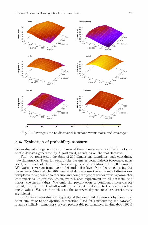
Fig. 10. Average time to discover dimensions versus noise and coverage.

5.6. Evaluation of probability measures

We evaluated the general performance of these measures on a collection of syn-thetic datasets generated by Algorithm 4, as well as on the real datasets.

First, we generated a database of 200 dimensions templates, each containingtwo dimensions. Then, for each of the parameter combinations (coverage, noiselevel) and each of these templates we generated a dataset of 1000 itemsets.We varied coverage from 1.0 to 0.6 and noise level from 0.0 to 0.4 using 0.1increments. Since all the 200 generated datasets use the same set of dimensionstemplates, it is possible to measure and compare properties for various parametercombinations. In our evaluation, we run each experiment on all datasets, andreport the mean values. We omit the presentation of confidence intervals forbrevity, but we note that all results are concentrated close to the correspondingmean values. We also note that all the observed dependencies are statisticallysignificant.

In Figure 9 we evaluate the quality of the identified dimensions by measuringtheir similarity to the optimal dimensions (used for constructing the dataset).Binary similarity demonstrates very predictable performance, having about 100%


precision in the case of 100% coverage, and then gradually loosing precision as theparameters become less favorable. The performance is still acceptable, at 75%,when we have high noise and low coverage. It is worth mentioning, that theaverage precision is exactly 100% (0% variance) in the case of 30% noise, whilethis is not true for 0% noise, as one might expect. This behavior can be explainedby the fact that our method does not include the length of itemsets into theoptimization criterion, and dimensions with smaller number of items and samecoverage are indistinguishable. On the other hand, noise helps to di!erentiatethe coverage for various itemset refinements, and facilitates selecting optimaland complete dimensions.

Cosine and Jaccard similarities show more dramatic decreases in perfor-mance. Moreover, the quality of identified dimensions is less than 100% withoutnoise, indicating that these measures are not suitable for itemset distributionsused in our datasets.

Matched and Weighted similarities perform more stable across the parametersranges (the similarity to optimal dimensions is always between 0.55-0.75), yetthey demonstrate a surprising behavior: precision grows with decreasing cover-age. This behavior, which is statistically significant, can be explained as follows.

– Minimizing entropy forces selecting very short (or very long) itemsets whichmaximize (or minimize) the probabilities;

– Both kinds of itemsets are very sensitive to co-occurrence;– Co-occurrence decreases proportionally with the coverage, while– Short itemsets have virtually the same coverage as the optimal ones and long

itemsets have even larger overall coverage (not in a binary sense), which de-creases slower than the actual binary coverage (used as a parameter);

– The optimality of longer itemsets grows when the di!erence between coverageand co-occurrence becomes more pronounced, with the decreasing coverage.

The above conditions result in selecting itemsets of proper length with the de-creasing coverage.

When we couple these similarity measures with the constraint based on min-imal coverage, we observe that quality improves (refer to the bottom graphs inFigure 9). The results show that we can achieve a better quality for high cover-age and low noise (up to 0.93). Quality for low coverage and high noise settingsdrops to 0.75, but remains always better than without constraining the itemsets.Note that in this case, we use Lemma 2 in order to stop refining the itemsets.Without this constraint, longer itemsets will be preferred due to the nature ofapplied probability measure, leading to solutions with less frequent and morenoisy itemsets. Even though Lemma 2 was proven for binary probabilities, wecan still use it here as a constraint, because it is based on the entropy measure,which is still indicative of the information content of dimensions (that is, cover-age) even when di!erent probability measures are applied. Note that instead ofLemma 2, we could use any hard constraint on coverage, in order to achieve asimilar behavior.

Figure 10 depicts the dependency of execution time to the same parame-ters of coverage and noise (the reported results are again averages over 200experiments). We observe that for binary similarity, the execution time dependsinversely on noise, and decreases along with coverage. Such improvement of exe-cution time, when the dataset quality decreases, has a simple explanation: noise-free and good-coverage dimensions require more iterations to converge, since till


the end of the optimization process multiple revisions of optimal dimensions arebeing concurrently optimized. On the other hand, the suboptimal dimensionsin noisy data move out of the allocated memory budget quite fast, and conse-quently, the algorithm converges faster. However, this does not imply that theidentified dimensions are better, as can be verified with the help of Figure 9.

As can be seen in Figure 10 (top right), our pruning technique based onLemma 2 demonstrates a considerable improvement of execution time for thebinary method (25% on average).

In terms of performance, matched and weighted similarities (refer to thebottom graphs of Figure 10) are faster than the rest, since in this case a memorybudget is very quickly flooded with various sub-optimal refinements, which cannot lead to any optimality improvements, therefore, preventing further iterations.

6. Conclusions and future work

Motivated by applications on repositories of annotated resources in the collabora-tive tagging domain, we introduce the problem of diverse dimension decomposi-tion in transactional databases. In particular, we adopt an information-theoreticperspective on the problem, relying on entropy for defining a single objectivefunction that simultaneously captures constraints on coverage, exclusivity andorthogonality.

We present an approximate greedy method for extracting diverse dimensions,that exploits the FP-tree representation of the input transactional dataset andclever pruning techniques. Our experiments on datasets of tagged resources fromflickr and del.icio.us confirm e!ectiveness and e#ciency of our proposal, andanalysis of titles from dblp demonstrates a possibility of applying diverse di-mension decomposition to text datasets as well. The assessment on syntheticand artificially noisy data confirms that our method is able to reconstruct the“true” dimensions, and it withstands noise.

In our future investigations, we plan to have a user study for evaluating thediscovered dimensions in di!erent domains. A possibility is also that of develop-ing a vertical application exploiting our method for mining diverse dimensionsin order to detect, in unsupervised and automatic fashion, collection of web siteswith diverse content from del.icio.us.

Acknowledgements. Francesco Bonchi and Aristides Gionis were partially sup-ported by the Torres Quevedo Program of the Spanish Ministry of Science andInnovation, co-funded by the European Social Fund, and by the Spanish Cen-tre for the Development of Industrial Technology under the CENIT program,project CEN-20101037, “Social Media” (www.cenitsocialmedia.es).

References

[1] A. J. Knobbe and E. K. Y. Ho, “Maximally informative k-itemsets and their e#cientdiscovery,” in KDD, T. Eliassi-Rad, L. H. Ungar, M. Craven, and D. Gunopulos, Eds.ACM, 2006, pp. 237–244.

[2] ——, “Pattern teams,” in PKDD, ser. Lecture Notes in Computer Science, J. Furnkranz,T. Sche"er, and M. Spiliopoulou, Eds., vol. 4213. Springer, 2006, pp. 577–584.

[3] N. Tatti, “Maximum entropy based significance of itemsets,” in Knowledge and InformationSystems (KAIS), vol. 17. Springer, 2008, pp. 57–77.


[4] ——, “Probably the best itemsets,” in KDD, B. Rao, B. Krishnapuram, A. Tomkins, andQ. Yang, Eds. ACM, 2010, pp. 293–302.

[5] J. V. Michael Mampaey, Nikolaj Tatti, “Tell me what i need to know: succinctly summa-rizing data with itemsets,” in KDD, 2011.

[6] H. Heikinheimo, E. Hinkkanen, H. Mannila, T. Mielikainen, and J. K. Seppanen, “Findinglow-entropy sets and trees from binary data,” in KDD, 2007.

[7] C. Zhang and F. Masseglia, “Discovering highly informative feature sets from data streams,”in DEXA, 2010.

[8] J. Han, J. Pei, and Y. Yin, “Mining frequent patterns without candidate generation,” inACM SIGMOD Conference, 2000, pp. 1–12.

[9] M. Tsytsarau, F. Bonchi, A. Gionis, and T. Palpanas, “Diverse Dimension Decompositionof an Itemsets Space,” in ICDM, 2011.

[10]B. Sigurbjornsson and R. van Zwol, “Flickr tag recommendation based on collective knowl-edge,” in WWW, 2008.

[11]R. van Zwol, B. Sigurbjornsson, R. Adapala, L. G. Pueyo, A. Katiyar, K. Kurapati, M. Mu-ralidharan, S. Muthu, V. Murdock, P. Ng, A. Ramani, A. Sahai, S. T. Sathish, H. Vasudev,and U. Vuyyuru, “Faceted exploration of image search results,” in WWW, 2010.

[12]M. Grahl, A. Hotho, and G. Stumme, “Conceptual clustering of social bookmarking sites,”in LWA 2007: Lernen - Wissen - Adaption, 2007.

[13]D. Ramage, P. Heymann, C. D. Manning, and H. Garcia-Molina, “Clustering the taggedweb,” in WSDM 2009: Proc. of the 2nd ACM Int. Conference on Web Search and DataMining, 2009.

[14]M. van Leeuwen, F. Bonchi, B. Sigurbjornsson, and A. Siebes, “Compressing tags to findinteresting media groups,” in CIKM, 2009.

[15]K. Morik, A. Kaspari, M. Wurst, and M. Skirzynski, “Multi-objective frequent termsetclustering,” in Knowledge and Information Systems (KAIS), vol. 30. Springer, 2012, pp.715–738.

[16]F. Bonchi, C. Castillo, D. Donato, and A. Gionis, “Topical query decomposition,” in KDD,2008.

[17]B. Carterette and P. Chandar, “Probabilistic models of ranking novel documents for facetedtopic retrieval,” in CIKM, 2009.

[18]R. L. Santos, C. Macdonald, and I. Ounis, “Exploiting query reformulations for web searchresult diversification,” in WWW, 2010.

[19]G. Capannini, F. M. Nardini, R. Perego, and F. Silvestri, “E#cient diversification of websearch results,” PVLDB, vol. 4, no. 7, pp. 451–459, 2011.

[20]F. Korn, A. Labrinidis, Y. Kotidis, and C. Faloutsos, “Quantifiable data mining using ratiorules,” VLDB J., vol. 8, no. 3-4, pp. 254–266, 2000.

[21]G. H. Golub and C. F. Van Loan, Matrix Computations, 3rd ed. The Johns HopkinsUniversity Press, October 1996.

[22]F. Verhein and S. Chawla, “Geometrically inspired itemset mining,” in ICDM, 2006, pp.655–666.

[23]T. M. Cover and J. A. Thomas, Elements of Information Theory. New York, NY, USA:Wiley & Sons, 1991.


Author Biographies

Mikalai Tsytsarau is a PhD candidate at the Database and Information Management GroupdbTrento of the department of Information Engineering and Computer Science DISI, at theUniversity of Trento, working with professor Themis Palpanas. He received his Master’s inComputer Science from the Belarusian State University and worked as a software engineer atEpam Systems. Mikalai also worked at Yahoo! Research and HP Labs as a visiting researcherand at Qatar Computing Research Institute as research associate. Mikalai’s main scientificinterests are in Data Management and Information Retrieval, with a focus on the web environ-ment. The list of his current research activities includes: large-scale Opinion Mining, ItemsetMining, Databases and Indexing structures. He also has an interest in Click-log Mining andEntity Re-ranking for search engines.

Francesco Bonchi is a senior research scientist at Yahoo! Research in Barcelona, Spain, wherehe is part of the Web Mining Group. His recent research interests include mining query-logs,social networks, and social media, as well as the privacy issues related to mining these kindsof sensible data. In particular, his main interest nowadays is to develop data mining methodsfor the analysis of information an influence spread. He gave a keynote talk at WI-IAT 2011on this topic. He has been program co-chair of the European Conference on Machine Learningand Principles and Practice of Knowledge Discovery in Databases (ECML PKDD 2010), andvarious workshops on social web mining, privacy and other topics in data mining.

Aristides Gionis is a senior research scientist in Yahoo! Research, Barcelona. He received hisPh.D from the Computer Science department of Stanford University in 2003 and until 2006he has been with the University of Helsinki. He is serving on the editorial boards of TKDEand KAIS and he has been in the program committee of numerous premier conferences. Hisresearch interests include algorithms for data analysis and applications in the web domain.

Themis Palpanas is a professor of computer science at the University of Trento, Italy. Hereceived his PhD degree from the University of Toronto, Canada. Before joining the Univer-sity of Trento, he worked at the IBM T.J. Watson Research Center. He has also worked forthe University of California, Riverside, and visited Microsoft Research and the IBM AlmadenResearch Center. He is the author of five US patents, three of which are part of commercialproducts. He has received three Best Paper awards (PERCOM 2012, ICDE 2010 and ADAP-TIVE 2009). He is serving on the Editorial Advisory Board of the Information Systems Journaland as an Associate Editor in the Journal of Intelligent Data Analysis. He is General Chair forVLDB 2013, has served on the program committees of several top database and data miningconferences.

Correspondence and o!print requests to: Mikalai Tsytsarau, via Sommarive 14, Povo (TN)

38123, Italy. Email: [email protected]

diverse dimension decomposition for itemset spacesdisi.unitn.it/~themis/publications/kais12.pdf ·...

Documents