Data Mining

Part 2. Data Preprocessing

2.4 Data Transformation

Data Transformation

Fall 2009

Instructor: Dr. Masoud Yaghini

Outline

� Introduction

� Normalization

� Attribute Construction

� Aggregation

� Attribute Subset Selection

Data Transformation

� Attribute Subset Selection

� Discretization

� Generalization

� References

Introduction

Data Transformation

Data Transformation

� Data transformation

– the data are transformed into forms appropriate for mining.

� Data transformation tasks:

– Normalization

– Attribute construction

Data Transformation

– Aggregation

– Attribute Subset Selection

– Discretization

– Generalization

Data Transformation Tasks

� Normalization

– the attribute data are scaled so as to fall within a small

specified range, such as -1.0 to 1.0, 0.0 to 1.0

� Attribute construction (or feature construction)

– new attributes are constructed and added from the given set

of attributes to help the mining process.

Data Transformation

of attributes to help the mining process.

� Aggregation

– summary or aggregation operations are applied to the data.

– For example, the daily sales data may be aggregated so as

to compute monthly and annual total amounts.

Data Transformation Tasks

� Discretization

– Dividing the range of a continuous attribute into intervals

– For example, values for numerical attributes, like age, may

be mapped to higher-level concepts, like youth, middle-

aged, and senior.

� Generalization

Data Transformation

� Generalization

– where low-level or “primitive” (raw) data are replaced by

higher-level concepts through the use of concept

hierarchies.

– For example, categorical attributes, like street, can be

generalized to higher-level concepts, like city or country.

Normalization

Data Transformation

Normalization

� An attribute is normalized by scaling its values so that

they fall within a small specified range, such as 0.0 to

1.0.

� Normalization is particularly useful for classification

algorithms involving

Data Transformation

– neural networks

– distance measurements such as nearest-neighbor

classification and clustering.

� If using the neural network backpropagation algorithm

for classification mining, normalizing the input values

for each attribute measured in the training instances

will help speed up the learning phase.

Normalization

� For distance-based methods, normalization helps

prevent attributes with initially large ranges (e.g.,

income) from out-weighing attributes with initially

smaller ranges (e.g., binary attributes).

� Normalization methods

Data Transformation

– Min-max normalization

– z-score normalization

– Normalization by decimal scaling

Min-max Normalization

� Min-max normalization

– performs a linear transformation on the original data.

� Suppose that:

– minA and maxA are the minimum and maximum values of

an attribute, A.

Data Transformation

� Min-max normalization maps a value, v, of A to v′ in

the range [new_minA, new_maxA] by computing:

AAA

AA

A

minnewminnewmaxnewminmax

minvv _)__(' +−

−

−=

Example: Min-max Normalization

� Let income range $12,000 to $98,000 normalized to

[0.0, 1.0].

� Then $73,000 is mapped to

716.00)00.1(000,12000,98

000,12600,73=+−

−

−

Data Transformation

716.00)00.1(000,12000,98

=+−−

z-score normalization

� In z-score normalization (or zero-mean

normalization)

– the values for an attribute, A, are normalized based on the

mean (Ā) and standard deviation (σA) of A.

� A value, v, of A is normalized to v′ by computing

Data Transformation

Example: z-score Normalization

� Let Ā = 54,000, σA = 16,000, for the attribute income

� With z-score normalization, a value of $73,600 for

income is transformed to:

225.1000,16

000,54600,73=

−

Data Transformation

000,16

Decimal Scaling

� Normalization by decimal scaling

– normalizes by moving the decimal point of values of

attribute A.

– The number of decimal points moved depends on the

maximum absolute value of A.

– A value, v, of A is normalized to v′ by computing

Data Transformation

– A value, v, of A is normalized to v′ by computing

– where j is the smallest integer such that Max(|v′|) < 1.

j

vv

10'=

Example: Decimal Scaling

� Suppose that the recorded values of A range from -986

to 917.

� The maximum absolute value of A is 986.

� To normalize by decimal scaling, we therefore divide

each value by 1,000 (i.e., j = 3) so that

Data Transformation

Normalization

� Note that normalization can change the original data

quite a bit, especially the z-score method.

Data Transformation

Attribute Construction

Data Transformation

Attribute Construction

� Attribute construction (feature construction)

– new attributes are constructed from the given attributes and

added in order to help improve the accuracy and

understanding of structure in high-dimensional data.

� Example

– we may wish to add the attribute area based on the

Data Transformation

– we may wish to add the attribute area based on the

attributes height and width.

� By attribute construction can discover missing

information.

Data Aggregation

Data Transformation

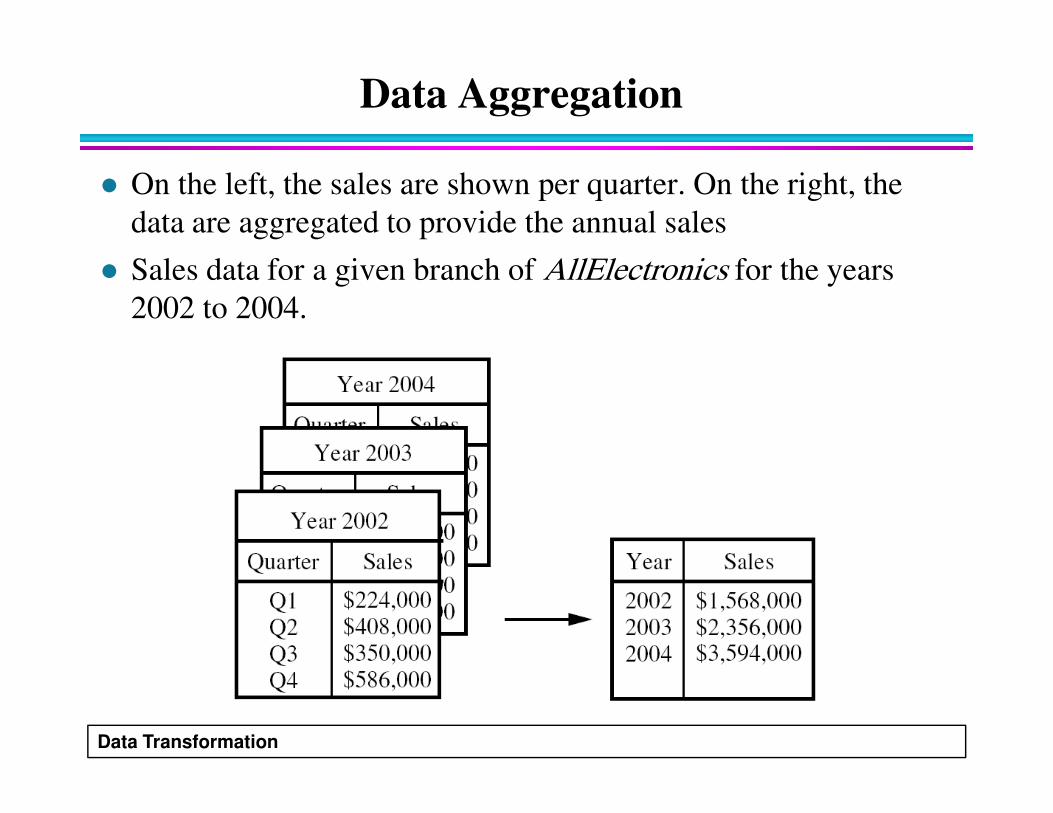
Data Aggregation

� On the left, the sales are shown per quarter. On the right, the

data are aggregated to provide the annual sales

� Sales data for a given branch of AllElectronics for the years

2002 to 2004.

Data Transformation

Data Aggregation

� Data cubes store multidimensional aggregated information.

� Data cubes provide fast access to precomputed, summarized data,

thereby benefiting on-line analytical processing as well as data

mining.

� A data cube for sales

at AllElectronics.

Data Transformation

Attribute Subset Selection

Data Transformation

Attribute Subset Selection

� Why attribute subset selection

– Data sets for analysis may contain hundreds of attributes,

many of which may be irrelevant to the mining task or

redundant.

� For example,

– if the task is to classify customers as to whether or not they

Data Transformation

– if the task is to classify customers as to whether or not they

are likely to purchase a popular new CD at AllElectronicswhen notified of a sale, attributes such as the customer’s

telephone number are likely to be irrelevant, unlike

attributes such as age or music_taste.

Attribute Subset Selection

� Using domain expert to pick out some of the useful

attributes

– Sometimes this can be a difficult and time-consuming task,

especially when the behavior of the data is not well known.

� Leaving out relevant attributes or keeping irrelevant

attributes result in discovered patterns of poor quality.

Data Transformation

attributes result in discovered patterns of poor quality.

� In addition, the added volume of irrelevant or

redundant attributes can slow down the mining

process.

Attribute Subset Selection

� Attribute subset selection (feature selection):

– Reduce the data set size by removing irrelevant or

redundant attributes

� Goal:

– select a minimum set of features (attributes) such that the

probability distribution of different classes given the values

Data Transformation

probability distribution of different classes given the values

for those features is as close as possible to the original

distribution given the values of all features

– It reduces the number of attributes appearing in the

discovered patterns, helping to make the patterns easier to

understand.

Attribute Subset Selection

� How can we find a ‘good’ subset of the original

attributes?

– For n attributes, there are 2n possible subsets.

– An exhaustive search for the optimal subset of attributes

can be prohibitively expensive, especially as n increase.

– Heuristic methods that explore a reduced search space are

Data Transformation

– Heuristic methods that explore a reduced search space are

commonly used for attribute subset selection.

– These methods are typically greedy in that, while searching

through attribute space, they always make what looks to be

the best choice at the time.

– Such greedy methods are effective in practice and may

come close to estimating an optimal solution.

Attribute Subset Selection

� Heuristic methods:

– Step-wise forward selection

– Step-wise backward elimination

– Combining forward selection and backward elimination

– Decision-tree induction

Data Transformation

� The “best” (and “worst”) attributes are typically determined

using:

– the tests of statistical significance, which assume that the attributes are

independent of one another.

– the information gain measure used in building decision trees for

classification.

Attribute Subset Selection

� Stepwise forward selection:

– The procedure starts with an empty set of attributes as the reduced set.

– First: The best single-feature is picked.

– Next: At each subsequent iteration or step, the best of the remaining

original attributes is added to the set.

Data Transformation

Attribute Subset Selection

� Stepwise backward elimination:

– The procedure starts with the full set of attributes.

– At each step, it removes the worst attribute remaining in the

set.

Data Transformation

Attribute Subset Selection

� Combining forward selection and backward

elimination:

– The stepwise forward selection and backward elimination

methods can be combined

– At each step, the procedure selects the best attribute and

removes the worst from among the remaining attributes.

Data Transformation

removes the worst from among the remaining attributes.

Attribute Subset Selection

� Decision tree induction:

– Decision tree algorithms, such as ID3, C4.5, and CART,

were originally intended for classification.

– Decision tree induction constructs a flowchart-like structure

where each internal (nonleaf) node denotes a test on an

attribute, each branch corresponds to an outcome of the test,

Data Transformation

attribute, each branch corresponds to an outcome of the test,

and each external (leaf) node denotes a class prediction.

– At each node, the algorithm chooses the “best” attribute to

partition the data into individual classes.

– When decision tree induction is used for attribute subset

selection, a tree is constructed from the given data.

– All attributes that do not appear in the tree are assumed to

be irrelevant.

Attribute Subset Selection

� Decision tree induction

Data Transformation

Discretization

Data Transformation

Discretization

� Data Discretization:

– Dividing the range of a continuous attribute into intervals

– Interval labels can then be used to replace actual data values

– Reduce the number of values for a given continuous

attribute

– Some classification algorithms only accept categorical

Data Transformation

– Some classification algorithms only accept categorical

attributes.

– This leads to a concise, easy-to-use, knowledge-level

representation of mining results.

Discretization

� Discretization techniques can be categorized based on

whether it uses class information, as:

– Supervised discretization

� the discretization process uses class information

– Unsupervised discretization

� the discretization process does not use class information

Data Transformation

� the discretization process does not use class information

Discretization

� Discretization techniques can be categorized based on

which direction it proceeds, as:

– Top-down

� If the process starts by first finding one or a few points (called split

points or cut points) to split the entire attribute range, and then

repeats this recursively on the resulting intervals

Data Transformation

– Bottom-up

� starts by considering all of the continuous values as potential split-

points,

� removes some by merging neighborhood values to form intervals,

and then recursively applies this process to the resulting intervals.

Discretization

� Typical methods:

– Binning

� Top-down split, unsupervised,

– Clustering analysis (covered above)

� Either top-down split or bottom-up merge, unsupervised

– Interval merging by χ2 Analysis:

Data Transformation

– Interval merging by χ2 Analysis:

� unsupervised, bottom-up merge

� All the methods can be applied recursively

� Each method assumes that the values to be discretized

Binning

� Binning

– The sorted values are distributed into a number of buckets,

or bins, and then replacing each bin value by the bin mean

or median

– Binning is a top-down splitting technique based on a

specified number of bins.

Data Transformation

specified number of bins.

– Binning is an unsupervised discretization technique,

because it does not use class information

� Binning methods:

– Equal-width (distance) partitioning

– Equal-depth (frequency) partitioning

Equal-width (distance) partitioning

� Equal-width (distance) partitioning

– Divides the range into N intervals of equal size: uniform

grid

– if A and B are the lowest and highest values of the attribute,

the width of intervals will be: W = (B –A)/N.

– The most straightforward, but outliers may dominate

Data Transformation

– The most straightforward, but outliers may dominate

presentation

– Skewed data is not handled well

Equal-width (distance) partitioning

� Sorted data for price (in dollars):

– 4, 8, 15, 21, 21, 24, 25, 28, 34

� W = (B –A)/N = (34 – 4) / 3 = 10

– Bin 1: 4-14, Bin2: 15-24, Bin 3: 25-34

� Equal-width (distance) partitioning:

Data Transformation

� Equal-width (distance) partitioning:

– Bin 1: 4, 8

– Bin 2: 15, 21, 21, 24

– Bin 3: 25, 28, 34

Equal-depth (frequency) partitioning

� Equal-depth (frequency) partitioning

– Divides the range into N intervals, each containing

approximately same number of samples

– Good data scaling

Data Transformation

Equal-depth (frequency) partitioning

� Sorted data for price (in dollars):

– 4, 8, 15, 21, 21, 24, 25, 28, 34

� Equal-depth (frequency) partitioning:

– Bin 1: 4, 8, 15

– Bin 2: 21, 21, 24

Data Transformation

– Bin 3: 25, 28, 34

Cluster Analysis

� Cluster analysis is a popular data discretization

method.

� A clustering algorithm can be applied to discretize a

numerical attribute, A, by partitioning the values of A

into clusters or groups.

Data Transformation

� Clustering takes the distribution of A into

consideration, as well as the closeness of data points,

and therefore is able to produce high-quality

discretization results.

Cluster Analysis

� Clustering can be used to generate a concept hierarchy

for A by following either a top-down splitting strategy

or a bottom-up merging strategy, where each cluster

forms a node of the concept hierarchy.

� In the former, each initial cluster or partition may be

further decomposed into several subclusters, forming a

Data Transformation

further decomposed into several subclusters, forming a

lower level of the hierarchy.

� In the latter, clusters are formed by repeatedly

grouping neighboring clusters in order to form higher-

level concepts.

Interval Merge by χχχχ2 Analysis

� ChiMerge:

– It is a bottom-up method

– Find the best neighboring intervals and merge them to form

larger intervals recursively

– The method is supervised in that it uses class information.

– The basic notion is that for accurate discretization, the

Data Transformation

– The basic notion is that for accurate discretization, the

relative class frequencies should be fairly consistent within

an interval.

– Therefore, if two adjacent intervals have a very similar

distribution of classes, then the intervals can be merged.

Otherwise, they should remain separate.

– ChiMerge treats intervals as discrete categories

Interval Merge by χχχχ2 Analysis

� The ChiMerge method:

– Initially, each distinct value of a numerical attribute A is

considered to be one interval

– χ2 tests are performed for every pair of adjacent intervals

– Adjacent intervals with the least χ2 values are merged

Data Transformation

– Adjacent intervals with the least χ2 values are merged

together, since low χχχχ2 values for a pair indicate similar class

distributions

– This merge process proceeds recursively until a predefined

stopping criterion is met (such as significance level, max-

interval, max inconsistency, etc.)

Generalization

Data Transformation

Generalization

� Generalization is the generation of concept hierarchies

for categorical data

� Categorical attributes have a finite (but possibly large)

number of distinct values, with no ordering among the

values.

Data Transformation

� Examples include

– geographic location,

– job category, and

– itemtype.

Example: Generalization

� A relational database or a dimension location of a data

warehouse may contain the following group of

attributes: street, city, province or state, and country.

� A user or expert can easily define a concept hierarchy

by specifying ordering of the attributes at the schema

level.

Data Transformation

level.

� A hierarchy can be defined by specifying the total

ordering among these attributes at the schema level,

such as:� street < city < province or state < country

References

Data Transformation

References

� J. Han, M. Kamber, Data Mining: Concepts and

Techniques, Elsevier Inc. (2006). (Chapter 2)

Data Transformation

The end

Data Transformation