do in-work tax credits serve as a safety net? · do in-work tax credits serve as a safety net?...

Do In-Work Tax Credits Serveas a Safety Net?

Marianne BitlerHilary HoynesElira Kuka

ABSTRACT

We test the EITC’s response to economic need. Using IRS data we exploitdifferences in timing and severity of economic cycles across states. Because theEITC requires earned income, there is a theoretical ambiguity in the credit’scyclicality. We find higher unemployment leads to increased likelihood of EITCrecipiency and in credit amounts received for married couples but hasinsignificant effects for single individuals. The EITC’s protective effects areconcentrated among skilled workers. The EITC mitigates income shocks formarried couples with children and groups likely to have moderate earnings, butdoes not for most recipients: single parents with children.

I. Introduction

The Earned Income Tax Credit (EITC) provides a refundable tax creditto lower-income working families through the tax system. As a consequence of legis-lated expansions in the EITC and the dismantling of welfare through the 1996 federalwelfare reform, the EITC is now the most important cash transfer program for low- andmoderate-income families (Bitler and Hoynes 2010). In 2012, the EITC reached 27.8

Marianne Bitler is a professor of economics at U.C. Davis and a faculty research associate at NBER.Hilary Hoynes is a professor of public policy and economics at U.C. Berkeley and a research fellow at NBER.Elira Kuka is an assistant professor at the Department of Economics, S.M.U. Funding for this project wasprovided by the Center for Poverty Research at UC Davis. The authors thank Dan Feenberg for help with theNBER SOI data. They are grateful to Sheldon Danziger, Laura Kawano, Yair Listokin, Jacob Goldin, DougMiller, and Bruce Meyer and participants at the NBERUniversities Research Conference “Poverty Inequalityand Social Policy,” the 2013 CELS Meeting, the 2014 AEA meetings, the 2015 SOLE meeting, APPAM,U.C. Berkeley, and U.C. Davis for useful comments. The authors also thank Janet Holtzblatt, Jeff Liebman,Laura Wheaton, and Ed Harris for help with constructing the “at-risk”’ population to accompany the datafrom SOI tax filing units. The data used in this article can be obtained beginning October 2017 throughSeptember 2020 from Hilary Hoynes, [email protected].[Submitted June 2014; accepted December 2015]; doi:10.3368/jhr.52.2.0614-6433R1ISSN 0022-166X E-ISSN 1548-8004ª 2017 by the Board of Regents of the University of Wisconsin System

Supplementary materials are freely available online at: http://uwpress.wisc.edu/journals/journals/jhr-supplementary.html

THE JOURNAL OF HUMAN RE SOURCE S � 5 2 � 2

million tax filers at a total cost of $64.1 billion. Almost 20 percent of tax filers receivethe EITC, and the average credit amount is $2,303. In contrast, in 2011, fewer than2 million families received cash welfare benefits, such as Temporary Assistance forNeedy Families (TANF), a 62 percent decline since 1994.One feature of a safety net program is that it raises disposable income for those at the

bottom of the income distribution. Using this definition, the EITC is the most importantsafety net program for low-income families with children: Based on the U.S. CensusSupplemental Poverty Measure, in 2013 the EITC (and the child tax credit) lifted 4.7million children out of poverty in a static sense, more than any other program (Short2014). Among all persons in the United States, only one government program lifts morepersons out of poverty: Social Security (Short 2014).A second key feature of a safety net program is that protection responds in times of

need. For example, a negative shock to family earnings as a result of job loss is mitigatedby social insurance benefits (such as unemployment compensation), public assistancebenefits (such as FoodStamps and, to a lesser extent, TANF), aswell as for higher incomefamilies, the progressive income tax system (Auerbach and Feenberg 2000). Kniesnerand Ziliak (2002) refer to these as providing “explicit” income-smoothing (transfers)and “implicit” income-smoothing (such as taxes). This stabilizing feature of the EITChas not been explored and is the focus of our work.We recognize that protecting againstshocks to income is not a stated goal of the EITC. But as the social safety net has beendramatically reformed with a new emphasis on in-work assistance (through welfarereform and the expansion of the EITC), it is important to evaluate the degree to whichthis central piece of the current safety net provides protection against shocks to income.To examine this issue, we use high-quality administrative data on tax returns from the

Internal Revenue Service (IRS), supplemented by data from the Current PopulationSurvey (CPS). Our empirical strategy relies on exploiting differences in the timing andseverity of economic cycles across states in a panel fixed effects model in order toestimate the relationship between business cycles and EITC recipiency and expendi-tures per potential filer. We measure the business cycle using the state unemploymentrate. Additionally, our results are robust to using the log of employment as a measure ofthe state business cycle, to using alternate functional forms for our outcome variables(logs), and to using different timing for the effects of the business cycle (lags).A defining feature of the EITC, and a general characteristic of “in-work” assistance

programs, is that positive earnings are required for a taxpayer to be eligible for the taxcredit. The prior literature has established that the EITC has led to sizable increases inthe employment rates of single mothers (Eissa and Liebman 1996; Meyer and Rosen-baum 2000, 2001; Hoynes and Patel 2015) and has led to modest reductions in theemployment of married women (Eissa and Hoynes 2004). Given the earnings re-quirement at the center of EITC eligibility, the response of EITC use to cycles (andeconomic need) is theoretically ambiguous, and may vary depending on where in theeligibility range tax filers lie. On the one hand, a downturn may lead to on-net higherrates of EITC participation—if the bulk of downturn-induced decreases in earningsmove taxpayers down into the EITC eligibility range. As wewill see below, this changeis most likely to occur for married couples with children and for the more highlyeducated among married and unmarried families with children. On the other hand,a downturn could lead to lower rates of EITC participation—if downturn-induced de-creases in employment bring earnings to zero for the majority of participants. This is

320 The Journal of Human Resources

most likely for unmarried tax filers with children and low education groups, based ontheir typical locations in the earnings distributions. Thus, our predictions are differentfor different groups, and the stabilization effect of the programmaywell not be uniform.This ambiguous role of the EITC in the presence of economic shocks has been

discussed by some legal scholars in the context of assessing the tradeoffs of efficiency,equity, and stabilization (Listokin 2012; Ryan 2014). And more generally, it is wellknown that a progressive income tax structure serves as an automatic stabilizer. (See, forexample, Auerbach and Feenberg 2000.) However, ours is the first study to empiricallyexamine the stabilizing feature of the EITC over the business cycle. Moreover, we arealso the first to explore differences across groups of taxpayers and to analyzewhether theoverall effects capture heterogeneous, offsetting effects across these groups, consistentwith their modal locations in the budget set, and to place such a discussion in the contextof static labor supply theory predictions.1 Our work also contributes to the empiricalliterature on the cyclicality of safety-net programs such as Food Stamps (for example,Ziliak et al. 2003; Bitler and Hoynes 2010), Aid to Families with Dependent Children(AFDC)/TANF (Blank 2001; Ziliak et al. 2000; Bitler andHoynes 2010), and other foodand nutrition programs (Corsetto 2012).Our main results use IRS Statistics of Income (SOI) microdata for tax years 1996-

2008.We choose this period because the EITC schedulewas relatively fixed during thisera, thereby allowing us to focus on how the program stabilizes income without con-founding these effects with policy-induced changes in participation and earnings. Wecollapse these data to cells defined by state, tax year, marital (filing) status, and numberof children. We then estimate models separately for different demographic groupsdefined by marital status and number of children.Our overall estimates suggest that, pooling all tax filers, EITC recipiency rates are

modestly countercyclical, with a one percentage point increase in the unemploymentrate—our primarymeasure of downturns in the business cycle—leading to a 1.8 percentincrease in the number of recipients per potential filer. However, this overall net effectmasks important differences across different family types and across groups with dif-ferent levels of education (and associated skill). We find that a higher unemploymentrate leads to a higher rate of EITC recipients per potential filer and higher expendituresper potential filer formarried coupleswith children. For example, a one percentage pointincrease in the unemployment rate leads to a 6.1 percent increase in the EITC recipiencyrate for this group. Filers without children, who are eligible for a much smaller credit,also exhibit countercyclical movements—a one percentage point increase in the un-employment rate leads to a 3.2 percent increase in the recipiency rate. These findingssuggest that for these groups an adverse labor market shock causes them tomove from apoint perhaps above the EITC eligibility limit (or along the phase-out region) to a lowerlevel in the earnings distribution relative to where they would have been absent theshock, leading to higher EITC participation rates and benefits. This thereby mitigatesthe adverse effects of labor market shocks.In contrast, the effect of business cycles on EITC use is negative (but due to large

standard errors, generally uninformative) for single tax filers with children, the largest

1. Jones (2015) uses linkedCPS-IRS data to look at the effect of theGreat Recession on the probability a familyhas both the earned income and the relevant family structure to make the family eligible to claim the EITC,finding results consistent with ours.

Bitler, Hoynes, and Kuka 321

group of recipients, whether measured by recipiency or expenditures. This negativepoint estimate is consistent with expectations for a “one earner” labor supply model—whereby an adverse labor market shock would eliminate family earnings, thus reducingthe likelihood of EITC participation. Further investigation shows that this statisticallyuninformative estimate for single tax filers with children masks protective effects forhigh-skill unmarried filers. On net, we find the EITC mitigates labor market shocks formarried couples with children and higher skill groupsmore generally, but does not do soon average for the largest group of recipients: single parents with children.To extend these findings and connect them to labor supply, we analyze the effects of

cycles on the distribution of earnings. In particular, we use the SOImicrodata to examineeffects of business cycles on the propensity to have earnings in various parts of theEITC-eligible range (the phase-in, flat and phase-out regions). Our results show that inrecessions, married couples’ earnings on net shift down into the EITC-eligible range.Single taxpayers also experience a shift down in earnings but most of this shift occurswithin the EITC schedule or in a way that moves them outside the region with taxliability (and into nonfiling status).To put these results in context, we compare our results to estimates of the cyclicality of

other key safety net programs including Unemployment Compensation, Food Stamps,and TANF. We show that the EITC exhibits less countercyclical movement than doTANF, Food Stamps, andUnemployment Compensation. Estimating similar models forthe same time period for recipients in each of these programs per capita, we find that aone percentage point increase in the unemployment rate leads to an increase in caseloadsper capita of 14.5 percent for Unemployment Insurance payments (UI), 8.4 percent forFood Stamps, and 7.7 percent for TANF, compared to 2.3 percent for the EITC.As a second way to put these results in context, we use the March Current Population

Survey to explore how the EITC affects the cyclicality of income. In particular, we esti-mate the effects of unemployment on poverty rates, using similar state panel data mod-els. Our baseline results use the official poverty measure, which depends on a family’spretax cash income.We then recalculate poverty rates after adding the EITC to pretax cashincome.Consistentwith the analysis of administrative SOI tax data, poverty fluctuates lessacross the business cycle when the EITC is included than when it is excluded, with thestrongest protective aspect of the EITC being among married couples with children.2

The remainder of this paper proceeds as follows. Section II outlines the EITC and therecent evolution of the safety net and discusses the relevant theoretical predictions.Section III discusses the data and Section IV presents our empirical model. The resultsare presented in Section V, sensitivity analysis is in Section VI, and we conclude inSection VII.

II. The EITC, the Prior Literature,and Theoretical Predictions

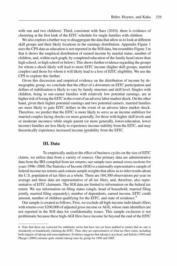
The U.S. safety net for low-income families has undergone a dramatictransformation in the past 15 years from being an out-of-work means-tested program toone requiring work. Many aspects of this transformation are illustrated in Figure 1. In

2. This comparison is static and does not reflect possible behavioral differences if theEITCprogramdid not exist.


this figure, we plot real per capita expenditures from 1980 to 2013 (2012 for the EITC)for the threemain cash or near-cash programs for low-income families with children: theEITC, Temporary Assistance for Needy Families, and Food Stamps (now called theSupplemental Nutrition Assistance Program or SNAP). The shaded regions are con-tractionary periods, annualized based on the National Bureau of Economic Research(NBER) recession dates and national unemployment peaks and troughs.3

The expansion of the EITC between 1986 and 1998, coupled with the decline in cashwelfare expenditures beginning with the welfare waivers of the early 1990s and con-tinuing through the 1996 federal welfare reform, led to the rise in the importance of theEITC and a corresponding fall in the importance of cash welfare. By 2012, spending onthe EITC was more than seven dollars for every dollar spent on TANF cash benefits. (In1994, on the eve of federal welfare reform, these programs were about equal in size.)This evolution represents a tremendous change in the safety net for low-income familieswith children—a transformation from out-of-work aid to in-work aid.

Figure 1Per Capita Expenditures on Cash and Near Cash Transfer Programs for Families($2012)Notes: Updated fromBitler andHoynes (2010) and the sources cited there. The shading indicates years of labormarket using annualized adaptation of NBER recession dating.

3. The official NBER recession dating is monthly; this figure presents annual data. We constructed an annualseries for contractions based on the official monthly dates, augmented by examination of the peaks and troughsin the national unemployment rate. See Bitler and Hoynes (2010) for more information on the annual dating.


As is suggested by Figure 1, the EITC is now one of the most costly cash or near-cashsafety net programs for low-income families with children. In 2012, the EITC wasreceived by 27.8million families (or,more accurately, tax filing units, which can includesingle individuals as well), at a cost of almost $64.1 billion. This amounts to an averagecredit of about $2,303 (IRS 2014).The EITC is distributed through the federal tax system, and the goal of the program is

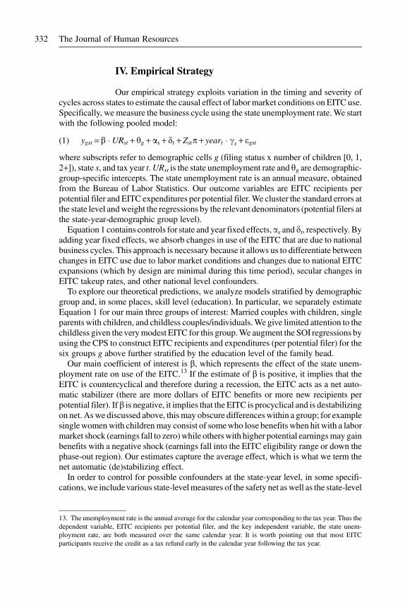
to increase the aftertax income of lower earning taxpayers, primarily those with chil-dren, while incentivizingwork. The EITC schedule has three regions. In the first, knownas the phase-in region, the credit is phased in at a constant rate: For each dollar earned,taxpayers currently receive 34-40 cents from the credit. In the second region, the flatregion, taxpayers receive the maximum amount of EITC benefit. In the phase-outregion, the credit is phased out at a constant rate: taxpayers lose 16-20 cents of credit foreach extra dollar earned. The potential income transfer is substantial—the maximumcredit for single filers with 2 or more children is $5,460 and the phase-out range extendsto earned income of $43,756 (2014 tax year). There are separate schedules for taxpayersdepending on the number of children and, in some years, marital status. Importantly,individuals without children are only eligible for a very small credit: In 2014 themaximum benefit for childless filers is $496, less than one-tenth the size of the credit fortwo-child families.4

Figure 2 plots the realmaximumbenefit by family size from1983–2014.Our analysisfocuses on the period 1996–2008, explicitly targeting a period of stability in the EITCtax schedule. We do this to isolate the effect of the business cycle. Unlike most of theEITC literature (see reviews by Hotz and Scholz 2003, Eissa and Hoynes 2006, andNichols and Rothstein 2015), we do not leverage policy variation in our research design.Our period lies after the large expansion due to OBRA93 and before the expansion thatwas part of the stimulus (in 2009).5

Table 1 provides descriptive statistics for EITC filers for 2008, the last year in ouranalysis period. The table shows that the recipients are split between singles withchildren (59 percent), married coupleswith children (19 percent), and taxpayerswithoutchildren (21 percent). In 2008, the average credit per filer was $2,613 for single parentswith children, $2,471 for married couples with children, and $253 for childless indi-viduals. Overall, the majority of the dollars spent on the program go to families withchildren: 74.1 percent of the credit dollars go to single filers with children and 23.2percent go to married filers with children. The small share of dollars claimed amongthose without children (2.7 percent) reflects their much lower potential credit amounts

4. Adjusted gross income (AGI) also plays a role in calculating EITC eligibility and benefits. First, AGI alsomust be less than the amount at the end of the phase-out region. Second, for filers in the phase-out region, theircredit is the lower of the credit calculated based on earned income and the credit based on AGI. When weanalyze EITC eligibility (as in Table 4 and Figure 5 below) we use only earned income and do not impose theAGI requirement. For more information on the EITC program, see Eissa and Hoynes (2006) and Hotz andScholz (2003).5. During the period we analyze, some minor expansions of the EITC occurred. Beginning in 2002, the phase-out range was increased for married taxpayers filing jointly. In our sample period, between 2002 and 2008, thephase-out range was extended by between $1000 (in 2002–2004) to $3000 (in 2008); in 2014 the phase-outrange was $5,430 higher. Additionally, in 2001 a “modified”AGI measure was replaced with AGI for analysisof eligibility and benefits in the phase-out region. In our analysis, time dummies will absorb the overall effectsof these minor policy expansions.


and participation rates. In fact, while among taxpayers with children takeup of the EITCis high (and has been steady) at about 75 to 80 percent (for example, Scholz 1994;Plueger 2009), EITC takeup for childless taxpayers is much lower at 56 percent.Predictions about how use of transfer and social insurance programs and regular

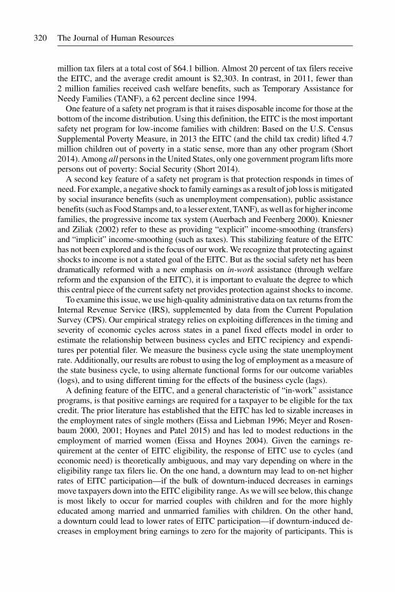
federal income tax payments will respond to economic downturns are straightforward;tax receipts should go down and transfers and UI use should go up. In contrast, theo-retical predictions about the effect of cycles on EITC use are ambiguous. Eligibility forthe EITC requires that earnings are strictly greater than zero and less than the amountdefining the end of the phase-out range. On the one hand, a downturnmay lead to higherrates of EITC participation and dollars received; if decreases in earningsmove taxpayersdown into the EITC eligibility range. On the other hand, a downturn could lead to lowerEITC participation and dollars received; if the main effect of the downturn is to causeindividuals to leave the labor force, reducing earnings to zero. The overall net effect ofeconomic downturns on EITC receipt and benefits depends on the breakdown betweentaxpayers brought into eligibility and those knocked out of the labor force and out ofeligibility.Figure 3 serves to sharpen these theoretical predictions for our main demographic

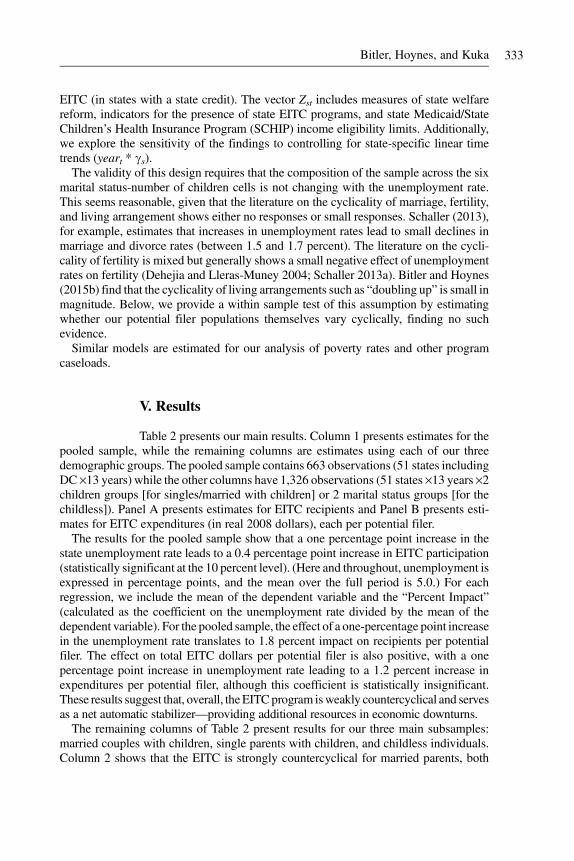
groups of interest. We present histograms for tax-return-reported earned income in2006, the peakyear just prior to the start of theGreat Recession (we describe the data and

Figure 2EITC Maximum Benefits by Number of Children ($2,012)Notes: Data on nominal EITC benefits are from the Tax Policy Center. Data on the CPI are from the BLS.


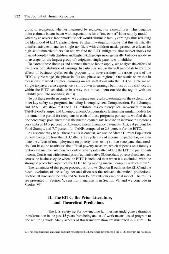
sample in detail below). We present the histograms for six demographic groups: singleindividuals with no children, married couples with no children, single with one child,married with one child, single with two or more children, and married with two or morechildren. For each, the dashed line shows the EITC schedule and we force the X- and Y-axes to have the same scale across all six graphs. We limit the sample in each case tothose returns with earned income between $1 and $60,000. We do not condition onreceipt of the EITC, but tabulate the total number of returns within each $1,000 bin ofearned income to see how these counts stack up across various points in the EITCschedule. On each graph, we also indicate the share of total filers for that demographicgroup that are excluded from the histogram (those filers with earned income that is £$0or >$60,000).Several observations can be drawn from these figures. First, they illustrate the vari-

ation in the generosity of the schedule across these six groups. The credit is substantiallylarger for families with children than for those without children, and the credit is largerfor families with two or more children than for one-child families. Second, the distri-bution of earned income for single families with children is shifted considerably to theleft of the distribution formarried familieswith children. Only 29 percent of singleswithone child and 18 percent of singles with two children have earnings higher than thetop of the phase-out range (compared to 76 percent and 75 percent for married families

Table 1Summary Statistics, EITC Recipients and Expenditures, 2008

A. Total Recipients and Expenditures

Total EITC recipients (millions) 24.4Total EITC expenditures (billions $2008) $50.5

B. Percent Distribution of Recipients, by Demographic Group

No children 21.9%Single with children 58.7%Married with children 19.4%

C. Percent Distribution of Expenditures, by Demographic Group

No children 2.7%Single with children 74.1%Married with children 23.2%

D. Average Credit Amount ($2008), by Demographic Group

No children $253Single with children $2,613Married with children $2,471

Notes: Data are from the 2008 Statistics of Income, which contains information on tax returns for tax year 2008(income earned during calendar year 2008). The sample excludes high-income earners, individuals livingabroad, late filers and married couples filing separately. Statistics are weighted to represent the population oftax filers.


Figure3

EITCElig

ibilityandtheEarnedIncomeDistributionin

2006

Notes:F

igures

show

theearned

incomedistributio

nfortax

year2006

with

theEITCscheduleoverlaid.Figures

onleftareforsinglefilers;figures

onrightareform

arried

filers.

Figures

inPanelsAandBareforfilerswith

nochild

ren;thoseinPanelsCandDareforfilerswith

onechild

,and

thoseinPanelsEandFareforfilerswith

2or

morechild

ren.

The

shareof

filerswith

negativ

eor

0incomeas

wellasthosewith

incomeabove$60,000areinthefigurenotes.Dataarefrom

Statisticsof

Incomefortax

year2006

(incom

eearned

during

calendar

year

2006).The

sampleexcludes

high-incom

eearners,individualsliv

ingabroad,latefilers,m

arried

couplesfilin

gseparately,and

child

less

elderly

taxpayers,which

aredefinedas

child

less

individualswith

positiv

egrossSocialS

ecurity

benefits.H

istogram

sareweightedto

representthe

populatio

nof

taxfilers.

(contin

ued)


Figure3

(contin

ued)


with one and two children). Third, consistent with Saez (2010), there is evidence ofclustering at the first kink of the EITC schedule for single families with children.We also explore a further way to disaggregate the data that allow us to look at different

skill groups and their likely locations in the earnings distribution. Appendix Figure 1uses the CPS data as education is not reported in the SOI data, but resembles Figure 3 inthat it shows the empirical distribution of earned income by marital status, number ofchildren, and, within each graph, by completed education of the family head (more thanhigh school, or high school or below). This shows further evidence regarding the groupsfor whom a shock likely will lead to more EITC income (higher skill groups, marriedcouples) and those for whom it will likely lead to a loss of EITC eligibility. We use theCPS to explore this further.Given this discussion and empirical evidence on the distribution of income by de-

mographic group, we conclude that the effect of a downturn on EITC participation anddollars of stabilization is likely to vary by family structure and skill level. Singles withchildren, being in one-earner families with relatively low potential earnings, are athigher risk of losing the EITC in the event of an adverse labormarket shock.On the otherhand, given their higher potential earnings and two potential earners, married familiesare more likely to gain EITC dollars in the event of an adverse labor market shock.Therefore, we predict that the EITC is more likely to serve as an income stabilizer formarried couples facing shocks (or more generally, for those with higher skill levels andor moderate incomes) while single parent (or more generally, lower-education, lowerincome) families are less likely to experience income stability from the EITC, and maytheoretically experience increased income instability from the EITC.

III. Data

To empirically analyze the effect of business cycles on the size of EITCclaims, we utilize data from a variety of sources. Our primary data are administrativedata from the IRS compiled from tax returns; our sample uses annual cross-sections foryears 1996-2008.The Statistics of Income (SOI) is a nationally representative sample offederal income tax returns and contain sampleweights that allow us to infer results aboutthe U.S. population of tax filers as a whole. There are 104,300 observations per year onaverage and these data are representative of all tax filers, and, therefore, also repre-sentative of EITC claimants. The SOI data are limited to information on the federal taxreturn. We use information on filing status (single, head of household, married filingjointly, married filing separately), number of dependents, earned income, EITC creditamount, number of children qualifying for the EITC, and state of residence.6

Our sample is created as follows. First, we exclude all high-income individuals (filerswith returns over $200,000 of adjusted gross income or AGI), whose state identifiers arenot reported in the SOI data for confidentiality issues. This sample exclusion is notproblematic because these high-AGI filers have income far beyond the end of the EITC

6. Note that these are corrected for arithmetic errors but have not yet been audited to ensure that no one ismistakenly or fraudulently claiming the EITC. Thus, they are representative of what tax filers claim, includingboth impacts of takeup and noncompliance. Evidence suggests that takeup is acyclical, and Scholz (1994) andPlueger (2009) estimate quite similar takeup rates by group for 1990 and 2005.


eligibility range.7 Second, we exclude individuals from Puerto Rico, the Virgin Islands,Guam, or U.S. citizens living abroad, as well as military personnel stationed abroad. Inthe SOI data, these filers all have the same geographic identifier, making it impossiblefor us to assign them to the labor market conditions that they face. Third, we drop latefilers, who are individuals filing tax returns in one year but whose returns correspond tosome previous tax year. By dropping late filers, we exclude 59,835 observations fromthe pooled 1996–2008 sample, which represents around 3 percent of the weightedsample. Below, we show in a robustness check that the results are not sensitive to thissample restriction. In addition, we excludemarried individuals filing separately, as thesefilers are not eligible for the EITC. We also exclude childless taxpayers age 65 andabove, given that EITC eligibility for filers without children is limited to those between25 and 64. Because age is not reported in the SOI data for our full-time period, we proxyfor those age 65 and above with those who claim Social Security Benefits.8

After these sample restrictions, we collapse the data to totals for cells based on year,state, marital status (married or single), and number of children (zero, one, or two ormore).9 For each cell, we calculate the total number of filers, the total number of filersclaiming the EITC, and the total amount of EITC benefits received; all as the weightedsums of these variables, using the sample weights provided in the SOI data.Our main outcome variables are the count of EITC recipients (where each unit

claiming the EITC is a recipient) and EITC expenditures, each measured per “potentialfiler.” Hence, we need to construct denominators of potential filers, the “at-risk” pop-ulations, in order to convert the administrative tax data counts to rates. To do so, we usedata from the March CPS to create population estimates (weighted using the familyhead’s weight) of the number of potential EITC filers in each state-year-marital status-number of children cell.10 TheMarch CPS is administered to most households inMarchand collects labor market, income, and program participation information for the pre-vious calendar year as well as demographic information from the time of the survey.Westart by using the CPS to identify the same six demographic groups used in the SOI:Each family (or subfamily) is assigned to a cell based on the marital status of the family

7. This group is relatively small, accounting for around 2.3 percent of the weighted sample.8. Social Security Benefits claimed on the tax return captures primarily retirement income but also includesSocial Security Disability income. We have cross-checked the data for 1994, where the SOI data provides avariable indicating the filer is age 65 and over, and found that, among filers who took no old age exemptions,only 4 percent declared Social Security benefits while among individuals that took one or two age exemption(for themselves and/or their spouse), the percent of filers with Social Security benefits was 60 percent and 68percent, respectively.9. We assign taxpayers to be married if they file married filing jointly, and single if the filer declared he/she isfiling singly or as a head of household (meaning single with dependent children). The number of children isassigned using the declared number of EITC-qualifying children. When tabulating total filers, we instead usethe number of child exemptions (because the number of EITC-qualifying children is obviously not observed fornon-EITC filers). Determinations for EITC-qualifying children and child exemptions are very similar andempirically more than 90 percent of EITC filers have equal values for the two measures. The main differencessince 2005 between the two definitions of children are that for exemptions, children must be U.S. citizens orpermanent residents and must satisfy the support test, while to be qualifying for the EITC children do not haveto satisfy the support test but have to live with the taxpayer in the U.S. for more than 50 percent of the time andhave a valid Social Security number.10. To be explicit, we pair estimates of the number of EITC filers for tax year X from the SOI (normally filed atthe beginning of year X + 1) with estimates of potential filers from CPS survey year X (measured in March ofyear X).


head and the family’s number of children. We identify children using the EITC filingrules: A child must be less than or equal to age 18, or he/she must be a full-time studentwhose age is less than or equal to 23, or he/she must be an individual who reports beingdisabled and that he/she cannot work. Potential filers among childless individuals arelimited to those units whose heads are aged 25–64 (following the EITC rules). Thesummary statistics for the sample are presented in Appendix Table 1.11

We also use the CPS to examine how the cyclicality of the EITC varies by skill group,which we measure using the education of the head (education is not observed in the taxdata). We use the NBERTAXSIM model to simulate EITC receipt and credit amounts.We then collapse the data to get average receipt rates and average EITC amounts perfamily for cells based on education (high school or below, some college or higher),marital status, number of children, state and year. Additionally, we use the CPS toexamine how the EITC affects the cyclicality of poverty, examining whether familieshave income below 50 percent, 100 percent, 150 percent, and 200 percent of the officialfederal poverty line. Official poverty status in the United States is determined bycomparing total pretax family cash income to poverty thresholds, which vary by familysize, number of children, and presence of elderly persons. In 2012, for example, thepoverty threshold for a family of three (one adult, two children) was $18,498. Notably,official poverty does not capture the tax system (such as the EITC) or the noncashtransfer system (such as Food Stamps).We calculate a second povertymeasurewhere theincome measure includes pretax income and TAXSIM simulated EITC. We also cal-culate cash poverty and cash plus EITC poverty using the official threshold for a familyof four and the equivalence scales from the Supplemental Poverty Measure that adjustfor unit size and composition (Short 2014).We calculate these four povertymeasures foreach family and then collapse the data to cells based on state, year, and family type.12

To put our results on the cyclicality of the EITC in further context, we estimate similarmodels for other safety net programs including AFDC/TANF, Food Stamps, andUnemployment Insurance (UI). As with the EITC, we analyze administrative counts ofcaseloads (here at the state-by-year level) that cover the same time period as our SOIdata. We choose to normalize these caseloads by total state population, given the dif-ferences in eligibility determinations and units across programs (and also present EITCresults normalized in the sameway). The AFDC/TANF and Food Stamps caseloads areaverage monthly measures (of families), while the UI data represent the total populationprobability of being on UI on a weekly basis (total weeks of any UI benefits claimeddivided by the product of 52 weeks times state population). These data can be found atthe U.S. Department of Health and Human Services (2013), U.S. Department ofAgriculture (2013), and the U.S. Department of Labor (2013).

11. As shown in Appendix Table 1, the resulting variable EITC recipients per at risk population of filers isabove 1 for single filers with children. Others have noted this high measured participation rate, which mayreflect complicated living arrangements (children moving between custodial parents during the year) ornoncompliance. We explore the sensitivity of our findings to how we construct these denominators below andfind that these choices make very little difference to our estimates.12. For creating the collapsed cells in the CPS, we use the weight of the individual denoted as the head (if afamily/subfamily) or the weight of the individual themselves (for the single childless filers).


IV. Empirical Strategy

Our empirical strategy exploits variation in the timing and severity ofcycles across states to estimate the causal effect of labor market conditions on EITC use.Specifically, we measure the business cycle using the state unemployment rate.We startwith the following pooled model:

(1) ygst =b � URst + hg + as + dt + Zstp+ yeart � cs + egstwhere subscripts refer to demographic cells g (filing status x number of children [0, 1,2+]), state s, and tax year t.URst is the state unemployment rate and yg are demographic-group-specific intercepts. The state unemployment rate is an annual measure, obtainedfrom the Bureau of Labor Statistics. Our outcome variables are EITC recipients perpotential filer and EITC expenditures per potential filer.We cluster the standard errors atthe state level andweight the regressions by the relevant denominators (potential filers atthe state-year-demographic group level).Equation 1 contains controls for state and year fixed effects,as and dt, respectively. By

adding year fixed effects, we absorb changes in use of the EITC that are due to nationalbusiness cycles. This approach is necessary because it allows us to differentiate betweenchanges in EITC use due to labor market conditions and changes due to national EITCexpansions (which by design are minimal during this time period), secular changes inEITC takeup rates, and other national level confounders.To explore our theoretical predictions, we analyze models stratified by demographic

group and, in some places, skill level (education). In particular, we separately estimateEquation 1 for our main three groups of interest: Married couples with children, singleparents with children, and childless couples/individuals.We give limited attention to thechildless given the verymodest EITC for this group.We augment the SOI regressions byusing the CPS to construct EITC recipients and expenditures (per potential filer) for thesix groups g above further stratified by the education level of the family head.Our main coefficient of interest is b, which represents the effect of the state unem-

ployment rate on use of the EITC.13 If the estimate of b is positive, it implies that theEITC is countercyclical and therefore during a recession, the EITC acts as a net auto-matic stabilizer (there are more dollars of EITC benefits or more new recipients perpotential filer). If b is negative, it implies that the EITC is procyclical and is destabilizingon net. Aswe discussed above, thismay obscure differenceswithin a group; for examplesinglewomenwith childrenmay consist of somewho lose benefits when hit with a labormarket shock (earnings fall to zero)while otherswith higher potential earningsmay gainbenefits with a negative shock (earnings fall into the EITC eligibility range or down thephase-out region). Our estimates capture the average effect, which is what we term thenet automatic (de)stabilizing effect.In order to control for possible confounders at the state-year level, in some specifi-

cations,we includevarious state-levelmeasures of the safety net aswell as the state-level

13. The unemployment rate is the annual average for the calendar year corresponding to the tax year. Thus thedependent variable, EITC recipients per potential filer, and the key independent variable, the state unem-ployment rate, are both measured over the same calendar year. It is worth pointing out that most EITCparticipants receive the credit as a tax refund early in the calendar year following the tax year.


EITC (in states with a state credit). The vector Zst includes measures of state welfarereform, indicators for the presence of state EITC programs, and state Medicaid/StateChildren’s Health Insurance Program (SCHIP) income eligibility limits. Additionally,we explore the sensitivity of the findings to controlling for state-specific linear timetrends (yeart * gs).The validity of this design requires that the composition of the sample across the six

marital status-number of children cells is not changing with the unemployment rate.This seems reasonable, given that the literature on the cyclicality of marriage, fertility,and living arrangement shows either no responses or small responses. Schaller (2013),for example, estimates that increases in unemployment rates lead to small declines inmarriage and divorce rates (between 1.5 and 1.7 percent). The literature on the cycli-cality of fertility is mixed but generally shows a small negative effect of unemploymentrates on fertility (Dehejia and Lleras-Muney 2004; Schaller 2013a). Bitler and Hoynes(2015b) find that the cyclicality of living arrangements such as “doubling up” is small inmagnitude. Below, we provide a within sample test of this assumption by estimatingwhether our potential filer populations themselves vary cyclically, finding no suchevidence.Similar models are estimated for our analysis of poverty rates and other program

caseloads.

V. Results

Table 2 presents our main results. Column 1 presents estimates for thepooled sample, while the remaining columns are estimates using each of our threedemographic groups. The pooled sample contains 663 observations (51 states includingDC ·13 years) while the other columns have 1,326 observations (51 states ·13 years ·2children groups [for singles/married with children] or 2 marital status groups [for thechildless]). Panel A presents estimates for EITC recipients and Panel B presents esti-mates for EITC expenditures (in real 2008 dollars), each per potential filer.The results for the pooled sample show that a one percentage point increase in the

state unemployment rate leads to a 0.4 percentage point increase in EITC participation(statistically significant at the 10 percent level). (Here and throughout, unemployment isexpressed in percentage points, and the mean over the full period is 5.0.) For eachregression, we include the mean of the dependent variable and the “Percent Impact”(calculated as the coefficient on the unemployment rate divided by the mean of thedependent variable). For the pooled sample, the effect of a one-percentage point increasein the unemployment rate translates to 1.8 percent impact on recipients per potentialfiler. The effect on total EITC dollars per potential filer is also positive, with a onepercentage point increase in unemployment rate leading to a 1.2 percent increase inexpenditures per potential filer, although this coefficient is statistically insignificant.These results suggest that, overall, theEITCprogram isweakly countercyclical and servesas a net automatic stabilizer—providing additional resources in economic downturns.The remaining columns of Table 2 present results for our three main subsamples:

married couples with children, single parents with children, and childless individuals.Column 2 shows that the EITC is strongly countercyclical for married parents, both


when measured by the recipiency rate and by total dollars per potential filer. A onepercentage point increase in the state unemployment rate leads to a 6.1 percent increasein the recipiency rate and a 5.7 percent increase in real credits per potential filer, withboth estimates significant at the 1 percent level. In addition, the EITC is estimated to beweakly countercyclical for childless individuals (Column 4)—a one percentage pointincrease in unemployment leads to a 3.2 percent increase in the recipiency rate (sig-nificant at the 10 percent level). In contrast, the largest group of EITC participants,single parents, has negative but statistically insignificant coefficients for the effect of thecycle on EITC use. These results, taken at face value, suggest procyclical movementsand income destabilization for single-parent families, although we note the confidenceinterval for the single-parent families is large.14

Table 2Effects of Unemployment Rate on EITC Recipiency Rates and Expendituresper Potential Filer

All Children, Married Children, Single No Children(1) (2) (3) (4)

Panel A: EITC Recipients per Potential Filer

Unemployment rate 0.386* 0.889*** -0.899 0.252*(0.219) (0.273) (1.329) (0.132)

Mean Y 0.220 0.146 0.868 0.079Percent impact (%) 1.8 6.1 -1.0 3.2Observations 663 1,326 1,326 1,326

Panel B: Real EITC Expenditures per Potential Filer ($2008)

Unemployment rate 550.6 1992.4*** -2457.2 47.3(608.2) (679.4) (3919.4) (46.0)


Notes: Data are from the 1996–2008 Statistics of Income, with denominators measuring the number ofpotential filing units from the CPS ASEC corresponding to the tax year (tax year X matched with survey donein year X). The sample excludes high-income earners, late filers, individuals living abroad andmarried couplesfiling separately. The dependent variables are total number of tax returns with EITC claims and real EITCexpenditures ($2008), each divided by the total number of potential filing units in each cell. All regressionsinclude controls for demographic characteristics, as well as state and year fixed effects. The results areweighted by the population of potential filers in each cell. The unemployment rate is measured in percentagepoints. Percent impact is calculated as the effect of a 1 percentage point (1 unit) increase in the unemploymentrate divided by the mean value of the dependent variable. Standard errors are clustered by state and shown inparentheses. *p < 0.10, **p< 0.05, ***p< 0.01.

14. In Appendix Table 2 we provide more detail by estimating models separately for all six demographicgroups (single or married, by zero/one/two or more children). Those results show similar responses for families


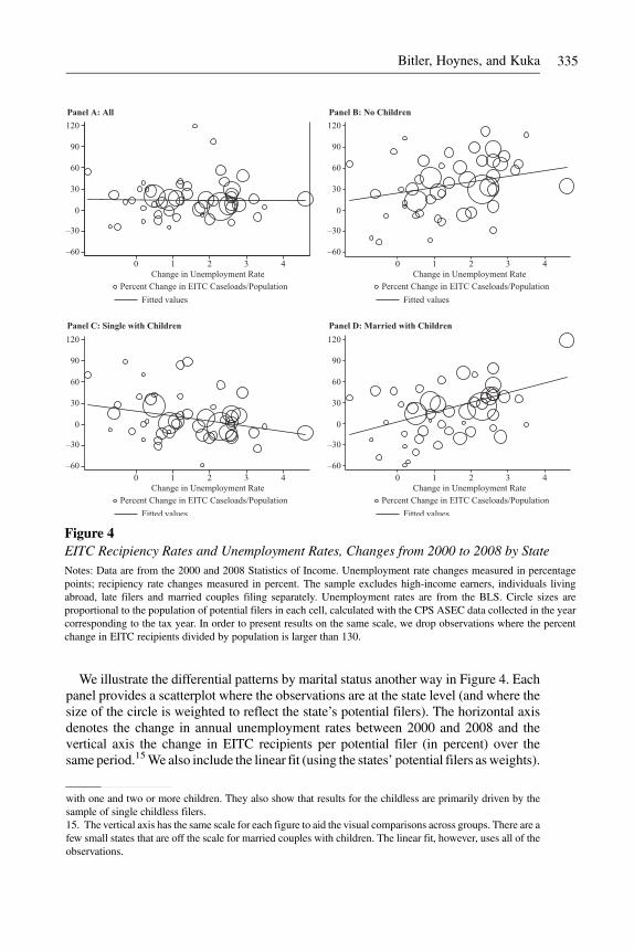
We illustrate the differential patterns by marital status another way in Figure 4. Eachpanel provides a scatterplot where the observations are at the state level (and where thesize of the circle is weighted to reflect the state’s potential filers). The horizontal axisdenotes the change in annual unemployment rates between 2000 and 2008 and thevertical axis the change in EITC recipients per potential filer (in percent) over thesame period.15We also include the linear fit (using the states’ potential filers asweights).

Figure 4EITC Recipiency Rates and Unemployment Rates, Changes from 2000 to 2008 by StateNotes: Data are from the 2000 and 2008 Statistics of Income. Unemployment rate changes measured in percentagepoints; recipiency rate changes measured in percent. The sample excludes high-income earners, individuals livingabroad, late filers and married couples filing separately. Unemployment rates are from the BLS. Circle sizes areproportional to the population of potential filers in each cell, calculated with the CPS ASEC data collected in the yearcorresponding to the tax year. In order to present results on the same scale, we drop observations where the percentchange in EITC recipients divided by population is larger than 130.

with one and two or more children. They also show that results for the childless are primarily driven by thesample of single childless filers.15. The vertical axis has the same scale for each figure to aid the visual comparisons across groups. There are afew small states that are off the scale for married couples with children. The linear fit, however, uses all of theobservations.


We present these “long-difference” scatterplots for four groups: The pooled sample,childless filers, single parents with children, andmarried couples with children. Consistentwith the regressions, the figures for married couples and childless filers show a positiverelationship between changes in unemployment rates and changes in EITC recipientsper potential filer. Single parents with children, however, exhibit a negative relationship,with rising unemployment rates associated with declining EITC recipiency rates.We extend our main results in several ways. First, we estimate models that allow for

differential effects in expansions and recessions. In all cases we fail to reject that thecoefficients are the same for the two periods, suggesting no evidence in favor ofasymmetric responses. Second, we explore a possible lag structure including the currentunemployment rate and a one-year lag of the unemployment rate, suggesting totaleffects quite similar to our main results.16 In addition, our results are robust to using thenatural log of employment as an alternative measure of the business cycle. These resultsare available in the online appendix.The results in Table 2 are consistent with our theoretical predictions of the effect of

local market conditions on EITC use by family type. Figure 3, presented above, illus-trates that only a relatively small share of the total filing population of single parentswithchildren has incomes above the EITC phase-out range. With such a large share of theirearned income distribution contained within the EITC eligibility range, it is likely that anegative labor market shock will lead to no change in EITC filing (a reduction inearnings within the eligibility range) or a reduction in EITC filing (due to job loss andearnings falling to zero). On the other hand, among married families with children, farmore than half the distribution lies above the phase-out range. A labor market shock tothis group, therefore, would be much more likely to lead to an increase in use of theEITC (by moving earnings into the EITC-eligible range). Given the presence of twopotential earners in the married households, it is less likely that a shock would lead bothmembers of the family to leave the labor market entirely.However, we acknowledge the distinct lack of precision in our main estimates for

single filers with children. The results in Table 2 show that the standard errors for thisgroup are more than four times the size of the standard errors for either of the other twogroups. These large standard errors render the results for this group uninformative, yetthis group represents almost three-quarters of EITC expenditures.We further investigatethis in several ways. First, we estimate models with the log of EITC recipients as thedependent variable, with and without a control for population.17 Second, we estimatemodels with the total state population as the denominator (rather than the potential filersin each demographic group). Table 3 presents these estimates. There are two importantfindings from this analysis. First, the percent effects are remarkably similar across thealternative specifications for all three marital status/children groups. Second, the stan-dard errors for single parents with children decline substantially (relative to the standarderrors for the other two groups) when we move away from the specifications with theCPS estimates of potential filers in the denominator.We conclude that ourmain findings

16. For married filers with children, we find some persistence of the effect: When we include the one year lagwe get 0.50 on UR(t) and 0.50 on UR(t-1). The results for single filers with children are both insignificant. Theeffects for filers without children are loaded onto the one period lag of the UR.17. Models with the log(EITC) as the dependent variable are estimated without weights. In practice, the resultsare not sensitive to weighting.


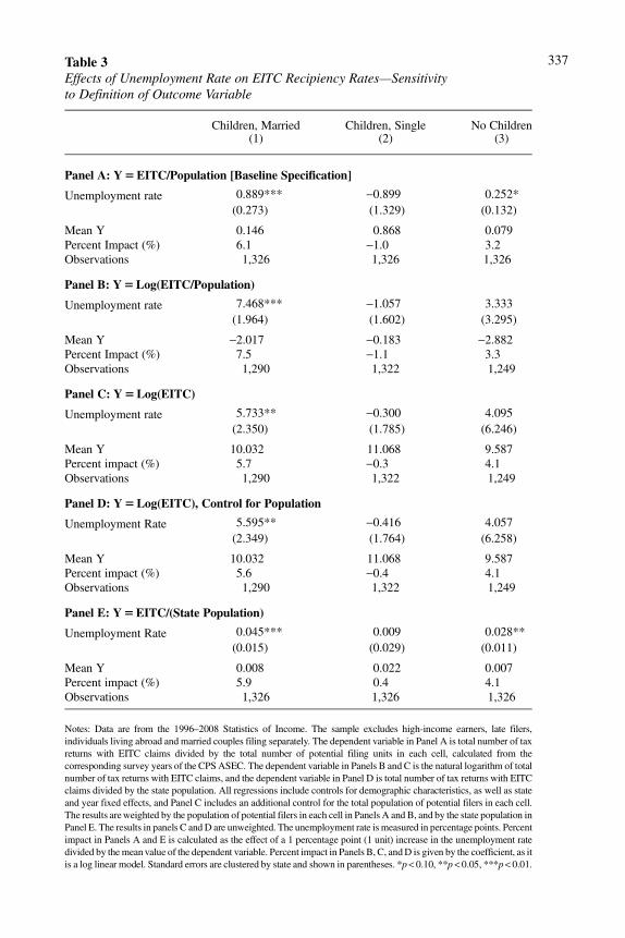
Table 3Effects of Unemployment Rate on EITC Recipiency Rates—Sensitivityto Definition of Outcome Variable

Children, Married Children, Single No Children(1) (2) (3)

Panel A: Y5EITC/Population [Baseline Specification]

Unemployment rate 0.889*** -0.899 0.252*(0.273) (1.329) (0.132)

Mean Y 0.146 0.868 0.079Percent Impact (%) 6.1 -1.0 3.2Observations 1,326 1,326 1,326

Panel B: Y5Log(EITC/Population)

Unemployment rate 7.468*** -1.057 3.333(1.964) (1.602) (3.295)

Mean Y -2.017 -0.183 -2.882Percent Impact (%) 7.5 -1.1 3.3Observations 1,290 1,322 1,249

Panel C: Y5Log(EITC)

Unemployment rate 5.733** -0.300 4.095(2.350) (1.785) (6.246)

Mean Y 10.032 11.068 9.587Percent impact (%) 5.7 -0.3 4.1Observations 1,290 1,322 1,249

Panel D: Y5Log(EITC), Control for Population

Unemployment Rate 5.595** -0.416 4.057(2.349) (1.764) (6.258)

Mean Y 10.032 11.068 9.587Percent impact (%) 5.6 -0.4 4.1Observations 1,290 1,322 1,249

Panel E: Y5EITC/(State Population)

Unemployment Rate 0.045*** 0.009 0.028**(0.015) (0.029) (0.011)

Mean Y 0.008 0.022 0.007Percent impact (%) 5.9 0.4 4.1Observations 1,326 1,326 1,326

Notes: Data are from the 1996–2008 Statistics of Income. The sample excludes high-income earners, late filers,individuals living abroad and married couples filing separately. The dependent variable in Panel A is total number of taxreturns with EITC claims divided by the total number of potential filing units in each cell, calculated from thecorresponding survey years of the CPSASEC. The dependent variable in Panels B and C is the natural logarithm of totalnumber of tax returns with EITC claims, and the dependent variable in Panel D is total number of tax returns with EITCclaims divided by the state population. All regressions include controls for demographic characteristics, as well as stateand year fixed effects, and Panel C includes an additional control for the total population of potential filers in each cell.The results areweighted by the population of potential filers in each cell in Panels A and B, and by the state population inPanel E. The results in panels C andD are unweighted. The unemployment rate is measured in percentage points. Percentimpact in Panels A and E is calculated as the effect of a 1 percentage point (1 unit) increase in the unemployment ratedivided by themeanvalue of the dependent variable. Percent impact in Panels B, C, andD is given by the coefficient, as itis a log linear model. Standard errors are clustered by state and shown in parentheses. *p< 0.10, **p< 0.05, ***p< 0.01.

337

are robust and the imprecision (for single parents with children) is likely driven by ourdenominator rather than the behavior of the EITC.We further explore the cyclicality of the EITC with data from the CPS, where we can

stratify our analysis using the education level of the family head (high school degree orless; some college or more). The results are shown in Table 4. Overall, for each of thethree demographic groups, those in the higher-education group exhibit statisticallysignificant stabilizing effects of the EITC. Both the higher- and lower-education groupsof married couples with children show such stabilizing effects. A one percentage pointincrease in the unemployment rate leads to a 6.3 percent increase in EITC claims perpotential filer for those with some college or more and a 3.8 percent increase for thosewith a high school degree or less. Single parentswith childrenwith some college ormorealso experience a stabilizing effect of the EITC; a one percentage point increase in theunemployment rate leads to a statistically significant 3.2 percent increase in EITCclaims per potential filer. Less educated single parents with children, by contrast, show

Table 4Effects of Unemployment Rate on CPS EITC Recipiency Rates—Heterogeneityby Education Level

All Children, Married Children, Single No Children(1) (2) (3) (4)

Panel A: Individuals with High School Degree or Less

Unemployment rate 0.511** 1.177*** -0.384 0.208(0.201) (0.310) (0.628) (0.170)


Panel B: Individuals with Some College or More

Unemployment rate 0.645*** 0.581*** 1.449*** 0.465***(0.109) (0.144) (0.385) (0.131)

Mean Y 0.110 0.092 0.458 0.045Percent impact (%) 5.9 6.3 3.2 10.3Observations 663 1,326 1,326 1,326

Notes: Data are from the 1997–2009 CPS ASEC, with denominators measuring the number of potential filingunits from the CPS ASEC corresponding to the tax year (tax year X matched with survey done in year X). Thedependent variable is total number of filers eligible for the EITC, as calculated by the NBER TAXSIM taxcalculator, divided by the total number of potential filing units in each cell. Education level is definedaccording to the family head. All regressions include controls for demographic characteristics, as well as stateand year fixed effects. The results are weighted by the population of potential filers in each cell. Theunemployment rate is measured in percentage points. Percent impact is calculated as the effect of a 1percentage point (1 unit) increase in the unemployment rate divided by the mean value of the dependentvariable. Standard errors are clustered by state and shown in parentheses. *p < 0.10, **p< 0.05, ***p < 0.01.


negative but statistically uninformative estimates. These results based on the CPS showthat the earlier SOI results reflect averages across skill subgroupswith different levels ofcyclicality.To more fully explore the differences by marital status and the connections to labor

supply predictions, we return to the SOI data and estimate our models on the number oftotal tax filers (rather than EITC recipients). In particular, we assign each filer to one ofsix earnings regions: 1) phase-in, 2) flat, 3) phase-out, 4) “near” phase-out (the region upto $25,000 above the end of the phase-out for families with children; or $15,000 abovefor the childless), 5) above the “near” phase-out, and 6) the remaining filers (negative orzero earned income). These regions are assigned using the appropriate tax schedule foreach group and tax year (for example, using the appropriate filing status and number ofdependents). It is important to point out that our SOI data are (necessarily) censored toinclude only those who file taxes. In particular, many families whose earnings drop tozero will not be required to file taxes.Table 5 presents estimates for total tax filers per potential filer (Panel A) and EITC-

eligible filers per potential filer (Panel B). The results show that single parents withchildren exhibit procyclical filing status—a one percentage point increase in the un-employment rate leads to a 1.6 percent reduction in the number of filers per potentialfiler. Childless filers also show procyclical filing status probabilities. In contrast, mar-ried couples show a very small and statistically insignificant relationship between cyclesand the probability of filing. The insensitivity of the propensity to file taxes amongmarried couples is consistent with their having two potential earners. The results forEITC-eligible filers per potential filer mirror the main results for EITC recipients inTable 2, with married couples showing a significant counter-cyclical EITC eligibility.Figure 5 presents similar results for filers with earnings in the phase-in, flat, phase-

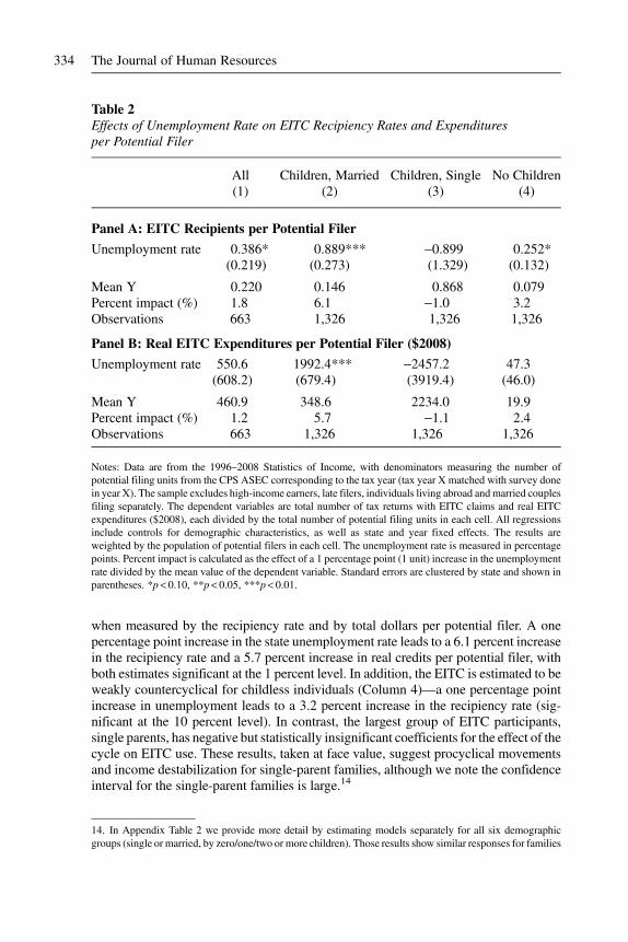
out, “near” phase-out, and above near phase-out regions. We plot the coefficient on theunemployment rate along with its 95 percent confidence interval for each outcome.(Appendix Table 6 contains the full set of coefficients and standard errors.) Figure 5ashows that, for married parents with children, an increase in the unemployment rateleads to a reduction in the propensity to have earnings in the highest category (above“near” phase-out) and an increase in the propensity to have earnings at all other, lower,levels. Notably, they have statistically significant increases for earnings in the phase-outand phase-in regions, consistent with the higher EITC participation and dollars dis-tributed per potential filer. The results for single parents with children, in Figure 5b,show that an increase in unemployment leads to reductions in the propensity to haveearnings in all regions above the very lowest (phase-in region). However, only thereductions for the near phase-out and above near phase-out are statistically significant.The propensity to have earnings in the phase-in increases (although not statisticallysignificantly so).The results in Tables 3 and 4 and Figure 5 serve to deepen our understanding of the

income stabilizing (or destabilizing) nature of the EITC. It also reveals that our findingsare consistent with a static labor supply model and potential earnings interpretation.One-earner familieswith relatively lowpotential earnings experience reductions in earn-ingswithin the EITC schedule. However, they also experience earnings losses that sendthem out of tax filing status. For two potential-earner families, whose baseline earningsare significantly shifted to the right of those for single-parent families, economic


downturns lead on net to a shift from being above the EITC-eligibility range down intothe EITC-eligibility range, with no corresponding change to tax-filing status. Singleparents with higher education (and potential earnings) exhibit responses more similar tothose of married couples, reflecting the fact that a decline in earnings could move theminto EITC eligibility (or to higher benefit levels as they move down the phase-out).To put these results in context, it is useful to compare these results to estimates for the

cyclicality of other key safety net programs. These results are presented in Table 6,where we compare results for the EITC to those for AFDC/TANF (Column 3), FoodStamps (Column 4), and UI (Column 5). For each model, the data are at the state-yearlevel covering the period 1996-2008, and we divide the various caseloads by the statepopulation. For the EITC, we present two measures—all EITC participants per capita

Table 5Effect of Unemployment Rate on Filing Propensity and EITC Eligible Filersper Potential Filer

Children, Married Children, Single No Children(1) (2) (3)

Panel A: Total Filers

Unemployment rate 0.189 -1.863* -1.776***(0.586) (1.064) (0.440)

Share of filers 1.00 1.00 1.00Mean Y 0.826 1.152 0.847Percent impact (%) 0.2 -1.6 -2.1Observations 1,326 1,326 1,326

Panel B: Filers in the Eligible Region

Unemployment rate 1.044*** -0.606 -0.396*(0.327) (1.053) (0.202)

Share of filers 0.24 0.74 0.24Mean Y 0.194 0.851 0.238Percent impact (%) 5.4 -0.7 -1.7Observations 1,326 1,326 1,326

Notes: Data are from the 1996–2008 Statistics of Income, with denominators measuring the number ofpotential filing units from the CPS ASEC corresponding to the tax year (tax year X matched with survey donein year X). The sample excludes high-income earners, individuals living abroad, late filers, married couplesfiling separately, and childless elderly taxpayers, which are defined as childless individuals with positive grosssocial security benefits. The dependent variable represents the number of filers in the SOI or the number offilers whose earned income puts them in the EITC eligible range, each divided by the total number of potentialfiling units in the demographic group. All regressions include controls for demographic characteristics, as wellas state and year fixed effects. The results are weighted by the population of potential filers in each cell. Theunemployment rate is measured in percentage points. Percent impact is calculated as the effect of a 1percentage point (1 unit) increase in the unemployment rate divided by the mean value of the dependentvariable. Standard errors are clustered by state and shown in parentheses. *p < 0.10, **p< 0.05, ***p < 0.01.


Figure 5Effect ofUnemployment Rate onLocation inEITCSchedule According toEarned IncomeNotes: Data are from the 1996–2008 Statistics of Income, with denominators measuring the number ofpotential filing units from the CPS ASEC corresponding to the tax year (tax year X matched with survey donein year X). The sample excludes high-income earners, individuals living abroad, late filers andmarried couplesfiling separately. Each point represents an estimated coefficient where the dependent variable is the number offilers whose earned income puts them in each EITC range, each divided by the total number of potential filingunits in the demographic group. All regressions include controls for demographic characteristics, as well asstate and year fixed effects. The results are weighted by the population of potential filers in each cell. Theunemployment rate is measured in percentage points. Standard errors are clustered by state.

341

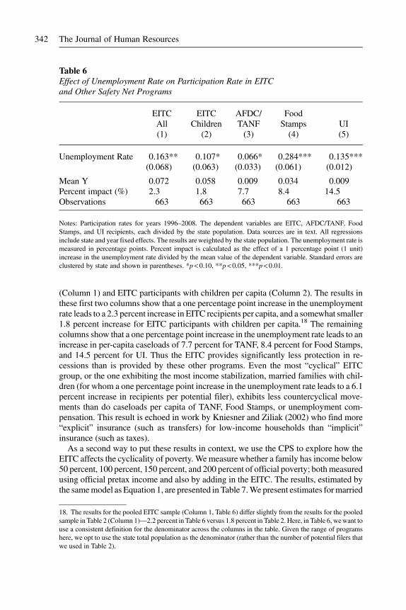
(Column 1) and EITC participants with children per capita (Column 2). The results inthese first two columns show that a one percentage point increase in the unemploymentrate leads to a 2.3 percent increase in EITC recipients per capita, and a somewhat smaller1.8 percent increase for EITC participants with children per capita.18 The remainingcolumns show that a one percentage point increase in the unemployment rate leads to anincrease in per-capita caseloads of 7.7 percent for TANF, 8.4 percent for Food Stamps,and 14.5 percent for UI. Thus the EITC provides significantly less protection in re-cessions than is provided by these other programs. Even the most “cyclical” EITCgroup, or the one exhibiting the most income stabilization, married families with chil-dren (for whom a one percentage point increase in the unemployment rate leads to a 6.1percent increase in recipients per potential filer), exhibits less countercyclical move-ments than do caseloads per capita of TANF, Food Stamps, or unemployment com-pensation. This result is echoed in work by Kniesner and Ziliak (2002) who find more“explicit” insurance (such as transfers) for low-income households than “implicit”insurance (such as taxes).As a second way to put these results in context, we use the CPS to explore how the

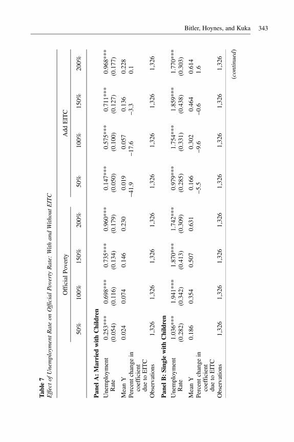
EITC affects the cyclicality of poverty. Wemeasure whether a family has income below50 percent, 100 percent, 150 percent, and 200 percent of official poverty; bothmeasuredusing official pretax income and also by adding in the EITC. The results, estimated bythe samemodel as Equation 1, are presented in Table 7.We present estimates formarried

Table 6Effect of Unemployment Rate on Participation Rate in EITCand Other Safety Net Programs

EITCAll

EITCChildren

AFDC/TANF

FoodStamps UI

(1) (2) (3) (4) (5)

Unemployment Rate 0.163** 0.107* 0.066* 0.284*** 0.135***(0.068) (0.063) (0.033) (0.061) (0.012)

Mean Y 0.072 0.058 0.009 0.034 0.009Percent impact (%) 2.3 1.8 7.7 8.4 14.5Observations 663 663 663 663 663

Notes: Participation rates for years 1996–2008. The dependent variables are EITC, AFDC/TANF, FoodStamps, and UI recipients, each divided by the state population. Data sources are in text. All regressionsinclude state and year fixed effects. The results are weighted by the state population. The unemployment rate ismeasured in percentage points. Percent impact is calculated as the effect of a 1 percentage point (1 unit)increase in the unemployment rate divided by the mean value of the dependent variable. Standard errors areclustered by state and shown in parentheses. *p< 0.10, **p< 0.05, ***p< 0.01.

18. The results for the pooled EITC sample (Column 1, Table 6) differ slightly from the results for the pooledsample in Table 2 (Column 1)—2.2 percent in Table 6 versus 1.8 percent in Table 2. Here, in Table 6, wewant touse a consistent definition for the denominator across the columns in the table. Given the range of programshere, we opt to use the state total population as the denominator (rather than the number of potential filers thatwe used in Table 2).


Tab

le7

Effectof

UnemploymentR

ateon

Official

PovertyRate:

With

andWith

outEITC

OfficialPoverty

Add

EITC

50%

100%

150%

200%

50%

100%

150%

200%

Pan

elA:Married

withChildren

Unemployment

Rate

0.253***

0.698***

0.735***

0.960***

0.147***

0.575***

0.711***

0.968***

(0.054)

(0.116)

(0.134)

(0.179)

(0.050)

(0.100)

(0.127)

(0.177)

MeanY

0.024

0.074

0.146

0.230

0.019

0.057

0.136

0.228

Percent

change

incoefficient

dueto

EITC

-41.9

-17.6

-3.3

0.1

Observatio

ns1,326

1,326

1,326

1,326

1,326

1,326

1,326

1,326

Pan

elB:Sing

lewithChildren

Unemployment

Rate

1.036***

1.941***

1.870***

1.742***

0.979***

1.754***

1.859***

1.770***

(0.282)

(0.342)

(0.413)

(0.309)

(0.285)

(0.331)

(0.438)

(0.303)

MeanY

0.186

0.354

0.507

0.631

0.166

0.302

0.464

0.614

Percent

change

incoefficient

dueto

EITC

-5.5

-9.6

-0.6

1.6

Observatio

ns1,326

1,326

1,326

1,326

1,326

1,326

1,326

1,326

(contin

ued)


Tab

le7

(contin

ued)

OfficialPoverty

Add

EITC

50%

100%

150%

200%

50%

100%

150%

200%

Pan

elC:Married

withChildren,

SPM

Equ

ivalence

Scales

Unemployment

Rate

0.245***

0.658***

0.735***

0.970***

0.134**

0.575***

0.757***

0.975***

(0.051)

(0.114)

(0.131)

(0.176)

(0.053)

(0.097)

(0.126)

(0.181)

MeanY

0.024

0.074

0.145

0.229

0.019

0.056

0.135

0.227

Percent

change

incoefficient

dueto

EITC

-45.3

-12.6

3.0

0.5

Observatio

ns1,326

1,326

1,326

1,326

1,326

1,326

1,326

1,326

Pan

elD:Sing

lewithChildren,

SPM

Equ

ivalence

Scales

Unemployment

Rate

1.124***

1.949***

1.883***

1.678***

1.141***

1.738***

1.955***

1.664***

(0.289)

(0.345)

(0.421)

(0.286)

(0.292)

(0.336)

(0.471)

(0.309)

MeanY

0.188

0.359

0.511

0.635

0.168

0.306

0.472

0.618

Percent

change

incoefficient

dueto

EITC

1.5

-10.8

3.8

-0.8

Observatio

ns1,326

1,326

1,326

1,326

1,326

1,326

1,326

1,326

Notes:D

ataarefrom

theCPSASECcalendaryears1996

–2008

andarecollapsed

atthedemographicgroup,stateandyearlevel.Childrenaredefinedfollo

wingthedefinitio

nfordependentchildren(sam

eas

child

renforEITCpurposes),andEITCeligibility

iscalculated

bytheNBERTA

XSIM

taxcalculator.P

anelsAandBinclud

etheresults

ofregressionsforb

eing

belowvariousmultip

lesof

theofficialpovertythreshold;PanelsCandDincludetheresults

ofregressionsforb

eing

belowvariousmultip

lesof

theofficial

povertythresholdforafamily

of4butincorporatetheequivalencescales

forfamilies

ofdifferentsizes

from

thenewSupplem

entalP

overty

Measure.A

llregressionsinclude

controls

fordemographic

characteristics,

aswellas

stateandyear

fixedeffects.

The

results

areweightedby

theweightedtotalnumberof

families

ineach

cell.

The

unem

ploymentrateismeasuredinpercentage

points.P

ercentchange

intheunem

ploymentcoefficientduetotheEITCiscalculated

asthepercentage

change

inthecoefficient

forbeingbelowtherelevant

multip

leof

thepovertythresholdbetweenthespecifications

forofficialpovertyandofficialpovertyafteradding

theEITCto

income.Standard

errorsareclusteredby

stateandshow

nin

parentheses.*p

<0.10,*

*p<0.05,*

**p<0.01.


couples with children and single parents with children. The first four columns showofficial poverty and confirm existing research documenting a positive relationship be-tween unemployment rates and poverty (Bitler and Hoynes 2010, 2016; Blank 1989,1993; Blank and Blinder 1986; Blank and Card 1993; Cutler and Katz 1991; Freeman2001; Gunderson and Ziliak 2004; Hoynes et al. 2006; Meyer and Sullivan 2011) withlarger cyclicality for single parents with children. For example, a one percentage pointincrease in unemployment leads to a 1.9 percentage point increase in official poverty(income below 100 percent poverty) for single families with children and 0.7 percentagepoint increase in official poverty for married couples with children. We repeat theexercise in Columns 5–8 but recalculate poverty after incorporating income from theEITC. Incorporating EITC income significantly reduces the cyclicality of poverty formarried couples. The effect of a one percentage point increase in unemployment isreduced by 42 percent for incomes below 50 percent of poverty, by 21 percent forincomes below 100 percent of poverty, by 6 percent for incomes below 150 percent ofpoverty, with a very small and insignificant effect on the propensity to have incomesbelow 200 percent of poverty. Given the relationship between poverty rates and theEITC schedule (see Appendix Figure 2), and given the results on earnings regions in theSOI data (Figure 3), this is precisely the pattern we would expect. In contrast, for singleparents with children, the EITC has minimal effects on the cyclicality of income. Theresults are very similar for the poverty measures using the supplemental poverty mea-sure equivalence scales (Panels C and D of the table).19

VI. Additional Results, Sensitivity Tests, and Threatsto Interpretation

The validity of our estimates requires that the changes in state unem-ployment rates are not reflecting other policies or trends at the state level that are bothcorrelated with the unemployment rate and drive EITC participation.We explore this inseveral ways, with results presented in Table 8. First, we control for other state policiesincluding welfare reform, indicators for the presence of state EITC programs, and stateMedicaid/SCHIP income eligibility thresholds. The results show (main results inColumn 1, results adding state-year controls in Column 2) that the results are highlyrobust to including these additional controls. Second, we include state-specific lineartime trends (in Column 3). Adding state linear trends changes the coefficients somewhat(leading to increases in the magnitude of impacts for single families with children anddecreases for married couples with children), but the qualitative conclusions are un-changed. Finally, we add both trends and controls, with the results in Column 4 beingvery close to those from specifications with state linear trends.The SOI data include “late filers” (file in year t a return for a year prior to t) and in our

main results we drop them from the sample. Ideally, we would reassign late filers to theappropriate filing year but for the last few years this reclassification is imperfect as not

19. This is a rather mechanical exercise, and in particular we are examining the cyclicality of poverty rates withand without the EITC in a static setting—assuming that nothing else in the family changes. Notably, this doesnot capture the channel whereby the EITC affects income and poverty through changing labor supply andearnings (Hoynes and Patel 2015).


all late filers have yet shown up. To explore the sensitivity to dropping late filers, weestimate models where we restrict the analysis to the years 1996–2004 (most late filingof taxes for tax year 2004 should have shown up by 2008) and examine the sensitivity toadding back in late filers. The results show that our results are not very sensitive to thissample exclusion. Another sensitivity test relates to our use of the CPS to constructpotential filers in the denominator of the EITC recipient and expenditure measures. Weexplore several different definitions for the denominators in an effort to best capture theEITC filing rules (especially as they relate to dependents) within the available CPS data.These results show very little difference across the alternative definitions for potentialfilers. The results for both of these sensitivity tests are available in the online appendix.In the previous section, we presented several results to corroborate our static

labor supply model and potential earnings interpretation of the results. However, an

Table 8Effect of Unemployment Rate on EITC Recipiency Rates, Sensitivityto Adding State-Year Controls

EITC Recipients/Population

(1) (2) (3) (4)

Panel A: Married with Children

Unemployment rate 0.889*** 0.897*** 0.474* 0.461*(0.273) (0.266) (0.262) (0.260)

Observations 1,326 1,326 1,326 1,326

Panel B: Single with Children

Unemployment rate -0.899 -0.812 -1.367 -1.563(1.329) (1.287) (1.591) (1.623)

Observations 1,326 1,326 1,326 1,326

Panel C: Childless Unemployment rate

0.252* 0.256* 0.150 0.119(0.132) (0.133) (0.145) (0.147)

Observations 1,326 1,326 1,326 1,326State policies Yes YesState linear trend Yes Yes

Notes: Data are from the 1996–2008 Statistics of Income, with denominators measuring the number ofpotential filing units from the CPS ASEC corresponding to the tax year (tax year X matched with survey donein year X). The sample excludes high-income earners, individuals living abroad, late filers and married couplesfiling separately. The dependent variables are total number of tax returns with EITC claims and real EITCexpenditures ($2008), each divided by the total number of potential filing units in each cell. All regressionsinclude controls for demographic characteristics, as well as state and year fixed effects. The results areweighted by the population of potential filers in each cell. The unemployment rate is measured in percentagepoints. Standard errors are clustered by state and shown in parentheses. *p< 0.10, **p< 0.05, ***p< 0.01.


alternative interpretation is that the differences across groups in the cyclicality of theEITC instead reflect differences in the cyclicality of labor supply across the groups. Theevidence from the substantial literature on the cyclicality of employment, hours, andearnings across demographic groups suggests otherwise. For example, Hoynes, Miller,and Schaller (2012) show that men, less-educated workers, and minorities are moresensitive to cycles than are others. We extend those findings and show that the em-ployment of single parents with children is more cyclical than is employment of marriedparents with children. (See online appendix.) We conclude that it is not greater cycli-cality among married couples that is generating our findings. Another possibility is thatour results reflect changes in marital status and fertility associated with the unem-ployment rate (which would affect the counts of potential filers across our demographicgroups). We explore this by testing whether the log of potential filers (by demographicgroup) is related to the cycle. We find very small and statistically insignificant effects ofunemployment on the log of potential filers, concluding that the potential for endoge-nous changes in marriage, fertility, and living arrangements is likely quite small andsecond order relative to the changes in labor supply across the cycle. (See onlineappendix.) A third possibility is that our results reflect cyclicality in tax compliance (ortakeup) as it relates to EITC filing. While this is inherently difficult to test, the fact thatwe find such similar effects between the SOI data (which embeds the empirical takeupand noncompliance) and the CPS (which embeds a 100 percent takeup and no non-compliance) leads us to conclude that this cannot be a major factor. In the end, we thinkthese analyses provide support for our interpretation—the results are due to differencesin labor supply responses and the distribution of skills across the demographic groups.

VII. Conclusion

Welfare reform and the expansion of the EITC have dramaticallychanged the landscape of redistribution policies for low-income families with childrenin the United States. This change has led to a movement away from “out of work”benefits, which have strong work disincentives, and an increase in “in work” benefits,which promote employment. This dramatic policy shift has been followed by otherdeveloped countries (Owens 2005).The research shows that these policies have been successful at increasing the em-

ployment of single mothers with children (Eissa and Liebman 1996; Meyer andRosenbaum 2000, 2001) and at removing children from poverty (Hoynes and Patel2015; Short 2014). In light of the importance of the EITC and the decline of TANF, inthis paper we evaluate whether the EITC satisfies a central tenet of safety net pro-grams—that they provide protection in times of economic need. Although we do not inany way claim that this protective role is an explicit goal of the EITC, evaluating thecurrent safety net in terms of whether and how it provides protection against incomelosses is important and understudied.We examine this issue by using administrative tax records to estimate the cyclicality

of the EITC over a period when EITC policy was relatively stable. We do so byleveraging substantial variation across states in the timing and severity of cycles, whichwemeasurewith the state unemployment rate. Our results show that for married couples


with children (and to a lesser extent the childless), EITC claims and income rise inrecessions, and thus the credit acts to mitigate income losses for this group. For thelargest group of EITC recipients, single mothers with children, there is a negative butgenerally statistically uninformative relationship between unemployment rates andEITCuse. These results can be understoodwithin the context of labor supply theory, andin particular connect to different predictions for how earnings change for one- versustwo-earner households, as well as to underlying differences in the distribution of incomeacross different family types. Further evidence breaking the data down by education ofthe filing unit head also supports these predictions.We do not view our results as suggesting that the EITC should be reformed to address

this limitation. Insuring against income shocks is not a stated goal of the EITC and its in-work structure yields important benefits in terms of increasing work and earnings andreducing poverty and income inequality. Yet we demonstrate that a consequence of thedecline of the move from out-of-work based assistance to in-work based assistance is lessprotection to income shocks for lower income groups (Bitler and Hoynes 2015a, 2016).In the Great Recession, this was countered to some extent by increases in Food Stampbenefits and unemployment insurance extensions, but these protections were temporary.As employment rates have increased among single women with children in response tothis change in the policy landscape, future work should examine whether and to whatextent Unemployment Insurance is providing job loss protection for this group.

References

Auerbach, Alan, and Daniel Feenberg. 2000. “The Significance of Federal Taxes as AutomaticStabilizers.” Journal of Economic Perspectives 14(3):37–56.

Bitler, Marianne, and Hilary Hoynes. 2010. “The State of the Safety Net in the Post-WelfareReform Era.” Brookings Papers on Economic Activity Fall 2010:71–127.

———. 2016. “The More Things Change, the More They Stay the Same? The Safety Net andPoverty in the Great Recession.” Journal of Labor Economics 34(1):part 2.

———. 2015a. “Heterogeneity in the Impact of Economic Cycles and the Great Recession:Effects Within and Across the Income Distribution.” American Economic Review. Papers andProceedings, 105(5):154–60.

———. 2015b. “Living Arrangements, Doubling Up, and the Great Recession: Was This TimeDifferent?” American Economic Review Papers and Proceedings 105(5):166–70.

Blank, Rebecca. 1989. “Disaggregating the Effect of the Business Cycle on the Distribution ofIncome.” Economica 56(222):141–63.

———. 1993. “WhyWere Poverty Rates So High in the 1980s?” In Poverty and Prosperity in theLate Twentieth Century, eds. Dimitri Papadimitriou, and Edward Wolff, 21–55. New York: St.Martin’s Press.

———. 2001. “What Causes Public Assistance Caseloads to Grow?” Journal of HumanResources 36(1):85–118.

Blank, Rebecca, and Alan Blinder. 1986. “Macroeconomics, Income Distribution, and Poverty.”In Fighting Poverty: What Works and What Doesn’t, eds. Sheldon Danziger, and DanielWeinberg, 180–208. Cambridge, Mass.: Harvard University Press.

Blank, Rebecca, andDavid Card. 1993. “Poverty, IncomeDistribution andGrowth: Are They StillRelated?” Brookings Papers on Economic Activity Fall 1993.


Corsetto, Lisa. 2012. “Food and Nutrition Program Cyclicality.” Mimeo. Davis: U.C. Davis.Cutler, David, and Lawrence Katz. 1991. “Macroeconomic Performance and the Disadvantaged.”Brookings Papers on Economic Activity Spring 1994.

Dehejia, Rajeev, andAdriana Lleras-Muney 2004. “Booms, Busts, andBabies’Health.”QuarterlyJournal of Economics 119(3):1091–130.

Eissa, Nada, and Hoynes, Hilary. 2004. “Taxes and the Labor Market Participation of MarriedCouples: The Earned Income Tax Credit.” Journal of Public Economics 88(9–10):1931–58.

———. 2006. “Behavioral Responses to Taxes: Lessons from the EITC and Labor Supply.” TaxPolicy and the Economy 20:74–110.

Eissa, Nada, and Jeffrey Liebman. 1996. “Labor Supply Response to the Earned Income TaxCredit.” Quarterly Journal of Economics 111(2):605–37.

Freeman, Richard. 2001. “The Rising Tide Lifts. ?” In Understanding Poverty, eds. SheldonDanziger and Robert Haveman, 97–126. Cambridge, Mass.: Harvard University Press.

Gundersen, Craig, and James Ziliak. 2004. “Poverty and Macroeconomic Performance AcrossSpace, Race, and Family Structure.” Demography 41(1):61–86.

Hotz, V. Joseph, and John Karl Scholz. 2003. “The Earned Income Tax Credit,” inMeans-TestedTransfer Programs in the United States, ed. Robert Moffitt, 141–98. Chicago: University ofChicago Press.

Hoynes, Hilary, DouglasMiller, and Jessamyn Schaller. 2012. “Who Suffers During Recessions?”Journal of Economic Perspectives 26(3): 27–48.

Hoynes, Hilary, Marianne Page, and Ann Stevens. 2006. “Poverty in America: Trends andExplanations.” Journal of Economic Perspectives 20(1):47–68.

Hoynes, Hilary, and Ankur Patel. 2015. “Effective Policy for Reducing Inequality? The EarnedIncome Tax Credit and the Distribution of Income.” NBER working paper 21340. Cambridge,Mass.: National Bureau of Economic Research.

Internal Revenue Service (IRS). 2014. Individual Income Tax Returns. Publication 1304 Rev 08-2014. Washington, D.C.: Internal Revenue Service.

Jones, Maggie. 2015. The EITC over the Business Cycle: Who Benefits? CARRAWorking Paper2014–15. Washington, D.C.: U.S. Census Bureau.

Kniesner, Thomas, and James Ziliak. 2002. “Explicit Versus Implicit Income Insurance.” Journalof Risk and Uncertainty 25(1): 5–20.

Listokin, Yair. 2012. “Equity, Efficiency, and Stability: The Importance of Macroeconomics forEvaluating Income Tax Policy.” Yale Journal on Regulation 378:45–78.

Meyer, Bruce, and Dan Rosenbaum. 2000. “A Making Single Mothers Work: Recent Tax andWelfare Policy and its Effects.” National Tax Journal 53(4):1027–62.

———. 2001. “Welfare, the Earned Income Tax Credit, and the Labor Supply of SingleMothers.”Quarterly Journal of Economics 116(3):1063–114.

Meyer, Bruce, and James X. Sullivan. 2011. “Consumption and Income Poverty over the BusinessCycle.” Research in Labor Economics 32, 51–82.

Nichols, Austin, and Jesse Rothstein. 2015. “The Earned Income Tax Credit.” NBER workingpaper 21211. Cambridge: Mass.: National Bureau of Economic Research.

Owens, Jeffrey. 2005. Fundamental Tax Reform: The Experience of OECD Countries. Back-ground Paper Number 47. Washington, D.C.: Tax Foundation.

Plueger, Dean. 2009.Earned Income Tax Participation Rate for Tax Year 2005.Washington, D.C.:Internal Revenue Service.

Ryan, Kerry. 2014. “EITC as Income (In)Stability?” 15 Florida Tax Review 583.Saez, Emmanuel. 2010. “Do Taxpayers Bunch at Kink Points?” American Economic Journal:Economic Policy 2(3): 180–212.

Schaller, Jessamyn. 2013. “For Richer if Not for Poorer? Marriage and Divorce over the BusinessCycle.” Journal of Population Economics 26(3): 1007–33.


———. 2013a. “Booms, Busts, and Fertility: Testing the Becker Model Using Gender-specificLabor Demand.” Working paper. Arizona: University of Arizona.

Scholz, John Karl. 1994. “The Earned Income Tax Credit: Participation, Compliance, and Anti-poverty Effectiveness.” National Tax Journal 47(1):63–87.

Short, Kathleen. 2014. The Research Supplemental Poverty Measure: 2013. Current PopulationReports P60–251. Washington, D.C.: U.S. Census Bureau.

U.S. Department of Agriculture. 2013. Caseload Data. Unpublished data provided by KatieFitzpatrick and John Kirlin of the Economic Research Service.

U.S. Department of Health and Human Services, Administration for Children and Families. 2013.Caseload Data. Washington, D.C.: U.S. Department of Health and Human Services, Office ofFamily Assistance. Available at: http://www.acf.hhs.gov/programs/ofa/data-reports/index.htm.

U.S. Department of Labor. 2013. 1979–2010 Data. Unpublished data provided by DOL OSEC.Washington, D.C.: U.S. Department of Labor.

Ziliak, James, David Figlio, Elizabeth Davis, and Laura Connolly. 2000. “Accounting for theDecline in AFDC Caseloads: Welfare Reform or the Economy?” Journal of Human Resources35(3):570–86.

Ziliak, James, Craig Gundersen, and David Figlio. 2003. “Food Stamp Caseloads over theBusiness Cycle.” Southern Economic Journal 69(4):903–19.


do in-work tax credits serve as a safety net? · do in-work tax credits serve as a safety net?...

Documents