Do Incentivized Managers Pay Their Workers Less?

Kuochih Huang∗

[Job Market Paper]Chyi-Horng Lu†‡

October 29, 2019

Abstract

Since the 1980s, Chief Executive Officers’ (CEO) pay has exploded, largely

in the form of equity-based incentive compensation such as stock awards and

options. Using a two-tiered principal-agent model, we show that aligning

managers’ incentives with shareholder interests through equity-based pay can

lower workers’ wages. Analyzing a sample that matches firm, manager, and

worker information in the U.S. economy over the period 1992-2016, we show

that higher equity-based pay is associated with lower average wages across

various measures of pays and model settings. Using a novel instrumental-

variable strategy based on a tax policy change, we provide evidence that

an increase in the CEO’s equity-to-salary ratio by one unit, say, from 1:1

to 2:1, leads to a 4% decline in the average wage. We also find that while

firms under all degrees of competition raise equity pay in response to the

policy change, the negative impact on wages is stronger when the degree

of competition is high, suggesting that competition does not substitute for

executive compensation but amplifies its effect.

Keywords: wage, corporate governance, executive compensation, product market competition

JEL Classification:

∗Lead author. Department of Economics, University of Massachusetts, Amherst. E-mail:kuochih@econs.umass.edu.†Department of Economics, National Taiwan University, Taipei.‡We thank the great help and insightful comments by Gerald Epstein, Ina Ganguli, Peter Skott, Kevin

Young, Taekjin Shin, William Lazonick, Wei-Kai Chen, Ming-Jen Lin, Chih-Sheng Hsieh, Wenting Ma.Kuochih thanks the financial supports from the Political Economy Research Institute fellowship, andthe UMASS Economics department summer research grant. All errors are ours.

1

1 Introduction

1.1 The equity-based compensation structure

Since the 1980s, as the wages of most workers have stagnated in the U.S., Chief Ex-

ecutive Officer (CEO) pay has exploded, largely in the form of equity-based incentive

compensation such as stock awards and options. Although the change in the CEO’s

compensation structure and the CEO-worker income gap have attracted a lot of atten-

tion, the literature usually analyzes the causes of patterns of CEO compensation and

workers’ wages separately; while the increase of CEOs compensation is attributed to

the competition for talent, managerial rent-seeking, tax policies and the need to provide

incentives for managers’ efforts under shareholders’ pressures,1 the stagnation of work-

ers wages is attributed to technological changes, globalization, declining union density,

etc. A critical issue has been largely omitted: does the change in CEOs’ compensation

structures make workers’ wages stagnate or decline? Specifically, do CEOs’ stock-based

pays, which have been the biggest part in the CEO’s compensation package since the

1980s, induce managers to cut workers’ wages?

The omission of empirical study on this issue is conspicuous against the theoretical

literature. Focusing on the conflicting incentives of “principals” (shareholders) and their

“agents” (managers), agency theory, which has been the major framework in the litera-

ture,2 claims that stock-based compensation helps to align the interests of shareholders

and managers, such that managers are less likely to take the “easy road”, paying high

wages as a comfortable way of minimizing conflicts; their energetic pursuit of self-interest

motivates them to cut wage costs and increase firm efficiency (Jensen and Meckling 1976;

Jensen & Murphy, 1990; Pagano & Volpin, 2005).3 In spite of the plausible prediction,

which we formalize in a simple model in Section 2, so far there is no empirical study on

the effect of managerial incentive compensation structure on workers wages in the U.S.

economy.

1 See, for example, Piketty & Saez (2003), Burkhauser, et al. (2012), and Bakija, Cole & Heim(2012) for the US case, and Bell & Van Reenen (2013) for the UK case.

2 See Shleifer & Vishny (1997), Murphy (2013), and Edmans, et al. (2017b) for reviews of theliterature.

3 Although a detailed analysis of the theoretical debates around the determinants of CEO compen-sation is beyond the scope of the present study, it’s interesting to mention that a variant of agencytheory, managerial rent-seeking theory (Bebchuk and Fried 2006), is based on the same principal-agentframework and shareholder primacy, but argues that excessive stock-based pay is actually a result ofmanagerial power, allowing managers to maximize their own interests at the expense of shareholdervalue. This theory proposes a better-designed incentive compensation and a stronger shareholder ac-tivism to discipline managers. Following this logic, however, we are not sure whether a rent-seekingmanager under stock-based compensation has an incentive to reduce wages or not. The proponents ofthe theory have been silent on this issue.

2

To fill the gap, this paper investigates the following question: Does equity-based

compensation incentivize managers to pay workers less? We first develop a simple two-

tier principal-agent model to show that because profit and therefore stock price are

influenced by the managers choice of monitor level, as long as the equity ratio is high

enough, the equity income may be sufficient to offset the cost of giving up the peaceful

life, such that the manager is willing to exercise high monitoring and reduce workers’

wages.

Next, we implement a set of analyses and a novel instrumental-variable strategy using

a tax policy change, finding that a higher equity-based pay, measured by Equity Frac-

tion (equity-based pays divided by the total compensation) or Equity Ratio (equity-based

pays divided by salary), consistently associates with lower wages. The effect persists even

when the equity-based pay is decomposed into stock awards and stock options, and also

when being combined into the performance pay as a whole. Evidence from our IV esti-

mation suggests that an one-unit increase in the CEO’s equity-to-salary ratio, say, from

1:1 to 2:1, will lead to a 4% reduction in the average wage. In addition to this baseline

result, we further show that this negative effect is more significant when the degree of

competition is high than low, implying that competition does not substitute compensa-

tion, but amplifies its effect by enlarging the gap between rewards under different profit

outcomes.

A major advance of this paper is the identification strategy based on a tax policy

change. The motivation of this effort is to identify causality beyond correlation, since

several omitted factors might affect both managers’ compensation structures and work-

ers’ wages and make them correlated. For example, a technology change may affect

the dynamics of both workers’ and managers’ labor markets, such that the firm can re-

duce ordinary workers’ wages while needing to provide more incentives to attract talented

managers. Alternatively, a firm with a worrisome business outlook may pay workers less,

and yet at the same time try to adopt new strategies by giving managers more equity

incentives. This paper addresses the issue by utilizing a change in the corporate-tax de-

ductibility of CEO’s salary brought by Section 162(m) of Internal Revenue Code in 1993.

Under this legislation, non-performance pays, mainly salaries, paid to top-five managers

above $1 million will be subjected to a 60% federal surtax. As a consequence, firms

switch to forms of performance pay, especially equity-based ones, to compensate their

managers while keeping salaries at or below the $1 million threshold. We use whether

the CEO’s salary falls into the treatment range around (and above) the threshold, and

the amount of salary, as instruments for changes in the CEO compensation structure

measured by the equity-based-pays-to-salary ratio. While this legislation and its effects

3

on CEO compensation structures had been studied by many, this paper is the first to

transform it into an instrument and identify the causal effects of compensation structure

on firm outcomes.

An important obstacle to any study on this issue in the U.S. economy is the lack

of micro-data that links the information of CEO compensation, firm characteristics and

workers’ wages precisely.4 To alleviate the obstacle, we focus on the average wage of

individual firm, and construct a firm-level sample by matching firms’ average wages and

other information (source: Compustat) with CEOs’ compensation structure (source:

Execucomp). We then link the data with workers’ characteristics calculated as the

weighted averages at the 2-digit industry level (sources: Current Population Survey

(CPS)). This results in a firm-level panel data set of the U.S. economy covering the

period 1992-2016, with variables of worker characteristics measured at the industry level.5

Supplementing to our baseline analyses, we also use other data in a set of robustness

tests (Section 3.3) to address several potential concerns, including the low report rate of

wage information in Compustat, composition changes due to offshoring, heterogeneity

between non-financial and financial sectors, and the industry-year-specific shocks.

1.2 Related literature and contributions of the paper

By showing that equity-based pay does induce managers to reduce workers’ wages in the

U.S., this paper makes several contributions to the following literature. First, this paper

is the first to study this question in the U.S. economy. To the best of our knowledge,

this issue had been addressed only partially by Cronqvist et al. (2009) for the Swedish

economy.6 In their analysis of Swedish data over the period 1995-2002, they find that

while CEOs with more voting rights pay their workers more, CEOs’ financial incentives

4 Most linked employer-employee data sets are merged at the establishment level using identifierssuch as Employer Identification Number (EIN). But a firm may have multiple establishments at variouslevels and use multiple EINs for different purposes. To the best of our knowledge, there is yet no simpleway to find all establishments for a given firm and merge the establishment-level data with firm’s balancesheet and CEO compensation data (Handwerker & Mason, 2013; 2014).

5 This approach of sample building is similar to many studies utilizing heterogeneities across in-dustries and using industry-level variables as their main explanatory variables and individual variablesas outcomes, such as the literature on inter-industry wage structure since Krueger & Summers (1988).Other examples include: Leonardi (2007) link individual data from CPS to firm data from Compustatat the industry level, to study the effects of industrial capital-labor ratio (capital per employee) onindividual wage dispersion; Lin & Tomaskovic-Devey (2013) match firm data from Compustat withindividual data from tax reports at the industry level, to study the effects of increasing dependence onfinancial income at the industry level on earnings dispersion among individual workers.

6 In the broader literature of corporate governance, for the U.S. economy, Bertrand & Mullainathan(1999; 2003) provide evidence over the period 1976-1995 showing that firms that face lower takeoverthreats due to anti-takeover legislation (and therefore managers are more entrenched) tend to pay theirworkers higher wages. Unfortunately they didn’t take into account the effects of managers’ compensa-tions.

4

(cash-flow rights, measured by the fraction of firms shares owned by the CEO) mitigate

such effects, putting downward pressures on workers wages. While their results are gen-

erally in line with ours, however, in an one-share-one-vote system that is common in the

U.S., a high managerial shareholding implies both strong controlling power and strong

financial incentives, which are predicted to have conflicting effects on wages. This may

cause ambiguities and hinder interpretations if we apply their measurement to the U.S.

case. Instead, this paper uses Equity Fraction and Equity Ratio as the main explanatory

variables to avoid the problem. In our analyses, the negative effects of Equity Frac-

tion and Equity Ratio on wages persist after controlling for managerial shareholdings.7

Moving beyond their analyses, we further examine the effects of various parts of execu-

tive compensation in detail, including stock award, stock option, performance pay as a

whole, and non-equity performance pay, and our examination include other high-ranking

managers’ compensations as well.

Second, due to the complexity in the process of determining executive compensation,

the empirical literature on the effects of executive compensation had been experiencing

difficulty in identifying causality, and just starts to overcome it in few recent studies.8

This paper joins in the rent trend to focus on the causal effect of executive compensation

structure on wages, using a novel identification strategy based on the IRC 162(m).

Third, a literature argues that changes in corporate governance do not matter in

competitive industries, because competition substitutes governance and always push

managers for efficiency. This thesis is supported by Giroud & Mueller (2010), in which

they find that changes in the anti-takeover regulation have no effect on firms’ perfor-

mances when competition is strong. However, we find a completely reversed pattern: the

negative impact of CEO equity pay is stronger when competition is strong, suggesting

that competition enlarges the gap between rewards under different outcomes and does

not substitute the effect of compensation but amplifies it.

Fourth, starting from Jensen & Meckling (1976), most theoretical literature on incen-

tive compensation focus on the managerial shareholding in the one-tier principal-agent

relationship between shareholders and managers.9 We argue that the effect of manage-

rial shareholding on wages is ambiguous, and focus on the compensation structure which

connects closely to our empirical analyses. In addition, in our two-tier principal-agent

model, we analyze the effect of compensation structure change using a multiplicative

7 Please see the results in Section 3.3.2.8 See Edmans, et al. (2017b) for a review of empirical literature on the effects of executive compen-

sations.9 The collusion model literature (Tirole, 1986; Pagano & Volpin, 2005) developed two-tier principal-

agent models, but did not move beyond the focus of managerial shareholding.

5

specification similar to Edmans, Gabaix & Landier (2008), rather than the additive one

typical in the literature, of CEO utility.

Fifth, in recent years, the increasing skepticism of equity-based pay, and of share-

holder primacy in general, have been focusing on other detrimental consequences: ex-

cessive risk-taking (Coles, et al., 2006; Chen, et al., 2006; Pathan, 2009; Bolton, et al.,

2015), increased stock buybacks at the expense of real investment and employment (La-

zonick, 2014; Almeida, et al., 2016; Edmans, et al., 2017a; Gutirrez & Philippon, 2016),

massive layoffs and outsourcing (Jung, 2015 & 2016; Dial & Murphy, 1995). This paper

contributes to this literature by providing the first evidence for the negative effects of

the incentive compensation on wages.

The rest of this paper is organized as follows. Section 2 develops a simple two-tiered

principal-agent model to clarify the main argument and prediction. Section 3 describes

the data and methods, presents our baseline results, and reports results from a set of

robustness tests. Section 4 explains the institutional background and the construct of

instrument, and presents evidence for causality based on the IV estimation. Section 5

looks closer at the effects of market competition on the relationship between the CEO’s

equity pay and workers’ wages. Section 6 concludes. Details of data sources, variable

measurements, and the results of robustness tests are reported in the Appendices.

2 A simple model of the effect of equity-based com-

pensation structure on wages

2.1 The argument and key features

The main argument of the model is that by increasing equity-based pays, measured by

Equity Fraction and Equity Ratio, the manager will be incentivized to reduce workers’

wages. In putting forward a tractable prediction, this section develops a simple two-tier

principal-agent model that first, specifies the manager’s incentives and the interactions

between the manager and the worker; and second, derives the measures of compensation

structures and analyzes the effects of changes in compensation structures on wages.

Three features distinguish the model from the literature. First, in analyzing the

interaction between the manager and the worker, this paper adopts a collusion model

following Tirole (1986) in which agents can make monetary or non-monetary side pay-

ments, i.e., private benefits.10 However, most collusion models start from analyzing the

10 The side payment (private benefit) and its effect on wages have been studied previously in thecontext of (anti-)takeover strategy used by the incumbent manager (Shleifer & Summers (1988); Pagano& Volpin (2005); Bertrand & Mullainathan (1999; 2003)). In contrast to the (anti-)takeover literature,in the model we abstract from the question of control, i.e., the power conflict between the shareholder

6

factors determining compensation, and aim to design an optimal contract from the prin-

cipal’s perspective. In contrast, this paper focuses on the consequence of the CEO’s

compensation structure, rather than the causes of it. In addition, as Tirole (1986) had

also warned that the model itself does not suggest whether the exchanges among agents

are welfare-enhancing (cooperation) or not (collusion), a discussion of the welfare out-

come requires a comprehensive general equilibrium model and a cost-benefit analysis

which go beyond the scope of this paper. This paper takes a more neutral and moderate

view, abstracting from the optimality question11 and focusing on the empirical prediction

to facilitate the empirical analysis.

The second feature of the model is the focus on the manager’s compensation struc-

ture, rather than his shareholding of the firm. The later has been the main measure of

executive incentives in the literature. For example, in Pagano & Volpin (2005), which de-

velops a model closest to mine, worker’s wages will be lower if the manager’s shareholding

is higher. An important reason for their focus on shareholding is to analyze the conflict

between the shareholder and the manager in controlling the firm, which is also the typical

concern of agency theory. In contrast, as implied in the first feature, this paper devi-

ates from the overwhelming concern of shareholder interest and the shareholder-manager

conflict. In addition, the shareholding measure may be inappropriate for our empirical

study, as it conflates controlling power and financial incentive in the one-share-one-vote

system, as explained in Section 1.2.

The third feature of the model is a multiplicative specification of CEO utility, rather

than the additive one typical in the literature. With multiplicative preferences, the utility

from private benefit is proportional to the CEO’s total compensation, and influences

naturally the fraction of equity-based pays needed to incentivize the manager to cut

wages. This specification is used in the macroeconomics literature on labor supply choice,

and is introduced into an analysis of CEO incentives by Edmans, Gabaix & Landier

(2008).

2.2 The model

The scenario of the model goes as follows. In a simple model of labor extraction and

collusion, the worker chooses the level of effort, and whether to give the manager a side

payment or not, depending on the level of monitoring chosen by the manager. The

manager chooses the level of monitoring, which relates directly to the worker’s wage

and the manager in controlling the firm.11 Therefore, for example, the simple model in this section does not explicitly specify the shareholder’s

utility function. The model also abstracts from some typical focuses of the literature on optimal com-pensation design like the uncertainty in measuring the manager’s effort.

7

level, accounting for the worker’s behaviors and the incentive compensation structure

designed by the shareholder. With the incidence of side payment depends on the level of

monitoring, the manager therefore faces a trade-off between the private benefit from the

side payment, and the value of the incremental reward brought by the choice of a higher

level of monitoring and regulated by the amount of equity in his compensation package.

The compensation structure measures how much the equity-based pay is needed for the

manager to offset the loss of private benefit. The model shows that with more equity-

based pays, measured by Equity Fraction and Equity Ratio, the manager will more likely

give up the private benefit and choose a higher level of monitoring, resulting in a lower

wage for the worker.

The presentation of the model proceeds in three steps. First, we solve the la-

bor extraction game to derive the wage function, and then specify the relation of the

wage/monitoring to the firm’s surplus and stock price. Second, we specify the payoff

and utility functions of the manager, and analyze his utility maximization by incorpo-

rating the participation and incentive-compatibility constraints, which naturally relate

to a threshold of equity-based compensation structure needed for inducing high monitor-

ing. Finally, we analyze the possible choice of compensation structure by shareholders

and its effect on workers’ wages, and explain the connection between two measures,

Equity Fraction and Equity Ratio, that will be used in the following empirical analyses.

2.2.1 Wage setting, the firm’s surplus, and stock price

In a simple model of labor extraction/monitoring, the worker can choose contributing

effort or not. If the worker contributes effort, his utility is w − c, and mw + (1 −m)w

otherwise, where w is the wage, w is the reservation wage, c is the cost of effort, m reflects

the strength or probability of monitoring. Therefore, the worker’s incentive compatibility

constraint is:

m(w − w) ≥ c, (1)

and the wage eliciting the worker’s effort is

w = w +c

m. (2)

There are two levels of output, yH and yL, corresponding to the worker’s effort and

no effort. Assume yH − yL > cm

, i.e., the increase in output is bigger than the cost of

eliciting effort by the wage, such that the manager and the shareholder will always want

to elicit effort. In this case, it is always the case that w = w+ cm, and the worker always

put effort and produce yH , while the manager can choose different levels of m and pay

different levels of w. Here we assume no link between monitor and outputs. This should

8

be treated as a conservative, “lower-bound” scenario, because should a higher monitor

level give rise to higher outputs and therefore higher profits, the manager’s opportunity

cost of having a peaceful life will be higher, and the manager would be more hostile at

all levels of equity ratio. For simplicity and focusing on the effect on the average wage,

we also assume the manager’s choices do not affect the number of workers and normalize

the number to one.

As we focus on the works of the manager and the worker, and abstract from other

production factors, the firm’s surplus, Π, is determined as

Π = yH − w − s, (3)

where s is the fixed salary for the manager. Specifically, denote ΠH and ΠL as the sur-

pluses produced when the manager chooses high and low levels of monitoring respectively

such that {ΠL = yH − (w + c

mL)− s if m = mL;

ΠH = yH − (w + cmH

)− s if m = mH .

Market then evaluates the firm’s surplus and projects onto a market price of the firm’s

stock as

p = p(Π(m)). (4)

For simplicity, we ignore here the complex and often imperfect process of stock market

evaluation, and assume that market can identify the effect of a manager’s action in the

sense that the function is monotonically increasing with Π. Without loss of generality,

the gap between pL and pH , which correspond to ΠL and ΠH , can be simplified as

pL = pH(1− λ), (5)

where 0 < λ < 1. With this simple representation, the change in the firm’s stock price

is regulated by λ, which is an indicator of price-to-surplus sensitivity created by the

manager’s monitoring. The more effective is the monitoring, the larger the indicator,

and therefore the larger difference between pL and pH .12 The value of the equity-based

pay is therefore regulated directly by the market evaluation of firm’s stocks which is

linked with the manager’s monitoring. While the manager can choose between high and

low levels of monitoring, the consequences of his choice to the firm’s surplus and stock

price are public knowledge and known beforehand.13

12 The price-to-surplus sensitivity can also vary with competition such that λ is larger under strongcompetition and smaller under weak competition. This interpretation is introduced in Section 5 wherewe analyze whether and how is the effect of equity pay on wages affected by competition.

13 This setting abstracts from the uncertainty in measuring the manager’s effort which has been afocus of the literature on optimal contract design. For recent theories incorporating this uncertainty inanalyzing the CEO’s overpay and rent extraction problem, please see Skott & Guy (2013) and Benabou& Tirole (2016).

9

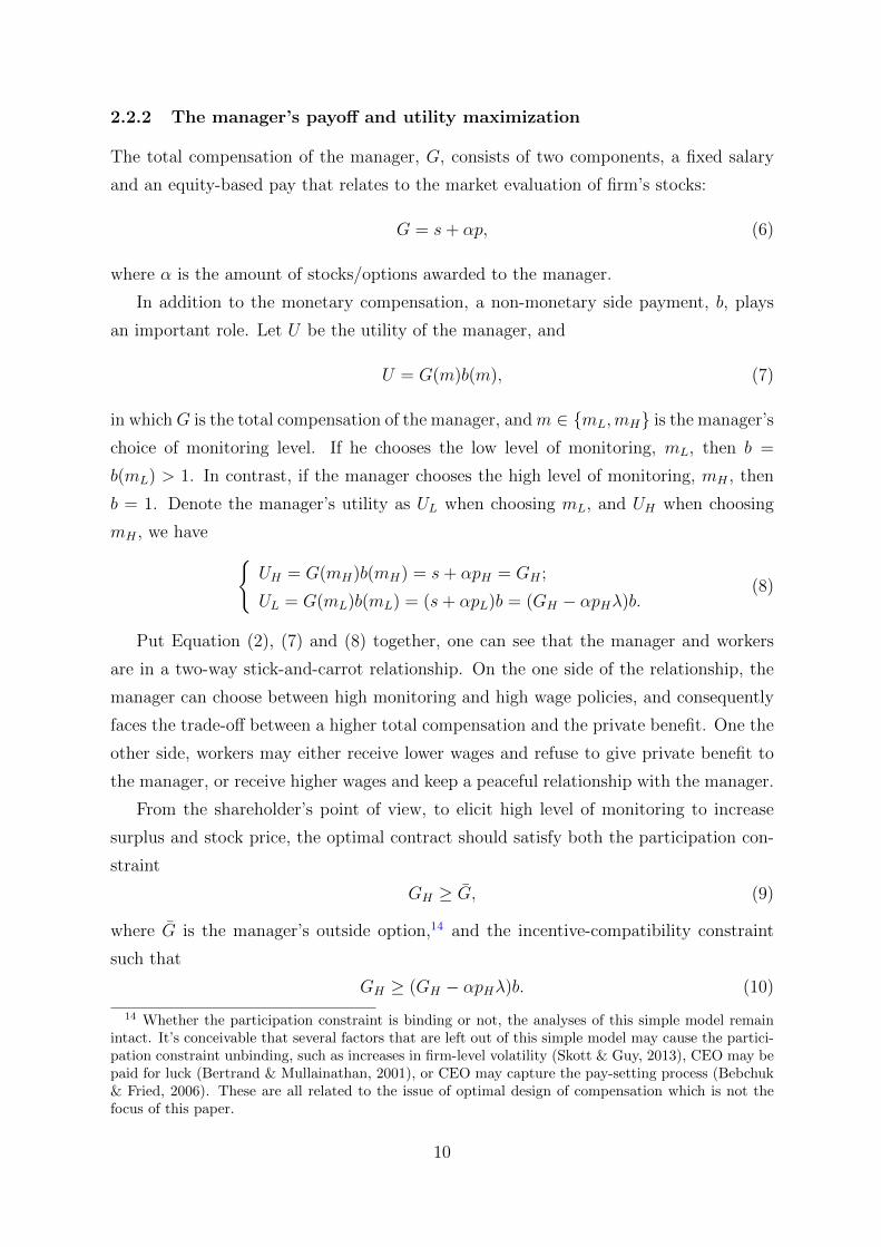
2.2.2 The manager’s payoff and utility maximization

The total compensation of the manager, G, consists of two components, a fixed salary

and an equity-based pay that relates to the market evaluation of firm’s stocks:

G = s+ αp, (6)

where α is the amount of stocks/options awarded to the manager.

In addition to the monetary compensation, a non-monetary side payment, b, plays

an important role. Let U be the utility of the manager, and

U = G(m)b(m), (7)

in whichG is the total compensation of the manager, andm ∈ {mL,mH} is the manager’s

choice of monitoring level. If he chooses the low level of monitoring, mL, then b =

b(mL) > 1. In contrast, if the manager chooses the high level of monitoring, mH , then

b = 1. Denote the manager’s utility as UL when choosing mL, and UH when choosing

mH , we have {UH = G(mH)b(mH) = s+ αpH = GH ;

UL = G(mL)b(mL) = (s+ αpL)b = (GH − αpHλ)b.(8)

Put Equation (2), (7) and (8) together, one can see that the manager and workers

are in a two-way stick-and-carrot relationship. On the one side of the relationship, the

manager can choose between high monitoring and high wage policies, and consequently

faces the trade-off between a higher total compensation and the private benefit. One the

other side, workers may either receive lower wages and refuse to give private benefit to

the manager, or receive higher wages and keep a peaceful relationship with the manager.

From the shareholder’s point of view, to elicit high level of monitoring to increase

surplus and stock price, the optimal contract should satisfy both the participation con-

straint

GH ≥ G, (9)

where G is the manager’s outside option,14 and the incentive-compatibility constraint

such that

GH ≥ (GH − αpHλ)b. (10)

14 Whether the participation constraint is binding or not, the analyses of this simple model remainintact. It’s conceivable that several factors that are left out of this simple model may cause the partici-pation constraint unbinding, such as increases in firm-level volatility (Skott & Guy, 2013), CEO may bepaid for luck (Bertrand & Mullainathan, 2001), or CEO may capture the pay-setting process (Bebchuk& Fried, 2006). These are all related to the issue of optimal design of compensation which is not thefocus of this paper.

10

By rearranging the conditions we obtain

αpH ≥ GHβ, (11)

where β = (1 − 1b) 1λ

denotes the equity-based pay fraction.15 Note that β = β(b, λ),

and βb > 0, that is, β needs to be higher if the private benefit b is larger, to induce the

manager to give up the private benefit and to choose high-level monitoring. In contrast,

βλ < 0, i.e., β can be lower and still generates enough rewards to the manager, if the

increase in the firm’s stock price brought by the manager’s monitoring effort being larger.

2.2.3 Two measures of compensation structure and the effect on wage

To link the theory with empirical analyses closely, we need to specify the two measures,

Equity Fraction and Equity Ratio, and restate the prediction. In Equation (9), by shifting

GH to the left, we can compute Equity Fraction, βF , that incentivizes the manager to

give up the private benefit and choose high monitoring:

m =

{mL if αpH

GH= βF < β;

mH if αpHGH

= βF ≥ β.(12)

An incentive compensation scheme set by the shareholder will aim to give the manager

a βF > β, which can be achieved by increasing α, given pH , β, and ∂βF

∂α> 0. A larger

α and therefore a larger βF will be more likely larger than β, such that the wage, w, to

be lower since cmH

< cmL

. That is, more equity-based pays, measured as higher Equity

Fraction, will leads to lower wages.16

Finally, it’s easy to see that the alternative measure, Equity Ratio, βR, works as a

proxy for Equity Fraction, since it is defined as

βR =αpHs

=βF

(1− βF ), (13)

where 0 ≤ βF ≤ 1 such that βR will move at the same direction as βF .

15 Here we restrict λ ≥ 1− 1b so that β ≤ 1.

16 Ordover & Shapiro (1984) and Skott & Guy (2007) had analyzed how the improvement of supervi-sion technology may reduce workers’ wages, as a process of power-biased technology change, or PBTC,vis-a-vis skill-biased technology change (SBTC). In the context of PBTC, the simple model presentedhere can be viewed as emphasizing that even after new supervision technology becomes available, afirm’s adoption of such technology still hinges on the manager’s incentives.

11

3 Basic Evidence on the Effects of Equity-Based Pays

on Wages

3.1 Data Sources and Measurements of Variables

The main dataset for following analyses is the firm-level sample based on the firm infor-

mation from Compustat, which is matched with CEOs’ information from Execucomp,

and workers’ characteristics from CPS measured at the industry level, over the period

1992-2016.17

Compustat provides balance sheet and other financial information for publicly-traded

firms in the U.S., which are collected from firms’ annual reports and other filings to the

SEC. Execucomp contains detailed information of top executives’ compensations, such as

salary, bonus, pension, stock award and stock option, and personal characteristics such

as gender and age, that are collected from firms’ annual proxy reports (DEF14A SEC

form). Current Population Survey (CPS) is a monthly survey of about 60,000 partici-

pating households, a sample representing the civilian non-institutional U.S. population,

conducted by the U.S. Census Bureau for the U.S. Bureau of Labor Statistics (BLS). We

use the Annual Social and Economic Supplement (ASEC), or the “March supplement”,

of the CPS which contains more demographic details than surveys in other months and

has been extensively used in the literature. A set of worker characteristics, such as gen-

der, race, education, union coverage, etc., are calculated as proportions at the 2-digit

SIC industry level. The details of matching methods are explained in Appendix 1.

3.1.1 The dependent variable: wage

Throughout the firm-level analyses, the dependent variable is log(yearly average wage)

of each firm-year observation. We use the labor and related expense (Compustat item:

xlr), subtract by the total amount of executive compensation of all top-five managers,

divide it by the number of employees (Compustst item: emp), and then take natural log.

The labor and related expense variable in Compustat includes salary and wage, other

benefit plans, payroll taxes, pension costs, profit sharing, and incentive compensation.

So this comprehensive measurement is less likely to be biased by the changes in the

composition of earning when, say, salary decreases while health insurance increases.

17 The matched data set begins at 1992 because Execucomp starts at 1992. A data set based onForbes surveys contains executive compensation data before 1992, but its measurements does not allowthe calculation of equity-based fraction of total compensation. Nonetheless we thanks Kevin Murphyfor sharing the data with me.

12

3.1.2 Explanatory variables: Equity Fraction and Equity Ratio

To capture the relative importance of equity-based pays to the manager, explanatory

variables consist of two measurements of executive compensation structure, Equity Frac-

tion and Equity Ratio. The former is measured as the sum of stock awards and stock

options values divided by the value of total compensation, and the later is measured as

the sum of stock awards and stock options values divided by the value of salary. As

explained in Section 2, a higher Equity Fraction or Equity Ratio, and therefore a heav-

ier weight of equity-based pays in the managerial compensation, is expected to align

managers’ interests closer with shareholders’ interests and lead to wage reductions.

In calculating the values of equity-based pays, we generally use the standard Black-

Scholes/fair-value measures to represent the ex ante evaluations of compensation values

at the beginning of a business year when executives plan their work. They are also

more available through the whole period, and widely used in the literature.18 Please see

Appendix 2 for more details.

Many studies investigate the differences between stock awards and stock options

regarding risk-taking behaviors. Based on the simple theory in Section 2, however, the

effects of stock awards and stock options on wages are indistinguishable and both are

negative. To check whether that’s the case empirically, we decompose equity-based pays

into stock awards and stock options, and calculate their fractions and ratios against total

compensation and salary respectively.

Although this paper focuses on equity-based pay, researchers and policy makers are

also interested in the performance pay in general which include bonus and various non-

equity incentives in addition of equity. Besides, it’s interesting to explore whether

equity-based and non-equity-based pays have different effects on wages. Since bonus

and non-equity incentives usually target certain accounting metrics rather than stock

performance, it’s likely that their effect on wages may be different from equity. We

therefore construct two additional variables: total performance pay fraction and ratio,

and non-equity performance pay fraction and ratio. The former includes equity-based

pays, bonus, and long-term incentive pay, while the later excludes equity-based pays.

Most literature on corporate governance/control focus only on CEOs. In a large firm,

however, given the complex process of decision making and division of labor, it’s not very

clear whether the CEO is the only person, or the most influential one, in determining

18 As reported in Hopkins & Lazonick (2016), the definitions and measurements of several compen-sation elements in Execucomp database had changed over the period, and some measures are availablefor shorter periods. In contrast to the Black-Scholes/fair-value measures, for example, the realized-value measures are ex post valuations whose values may be relatively uncertain to the executives at thebeginning of a year, and they are available only after 2006.

13

the wage policy. To investigate this issue, we calculate Equity Fraction and Equity Ratio

for other high-rank managers, and create corresponding non-CEO variables by taking

averages across these managers.

3.1.3 Control variables

We control for four groups of factors including manager, firm, and worker characteristics,

and a set of fixed effects.

Manager characteristics. Aside from the compensation structures, managers’ powers

in controlling the firm vis-a-vis shareholders are relevant to the determination of wages,

as the theory predicts that a powerful manager tends to collude with workers by paying

them higher wages. Together with the compensation structures, they measure the extent

and mechanisms of alignment between the interests of executives and shareholders in

the context of principal-agent relationship. We include two measurements to proxy for

the managers’ controlling powers. First, CEO-chair duality. The board of directors is

supposed to select and supervise the CEO. If the CEO is also the board chair, the check

and balance effect is weakened, giving the CEO more discretionary power, though not

necessarily more independence from shareholders. Second, whether the CEO is hired

from outside. A CEO promoted through the long ladder within a firm may have more

connections and influences among his or her coworkers, while an externally-hired CEO

may rely more on the supports of shareholders. A large literature finds that women make

economic decisions differently (Croson & Gneezy, 2009), so we include managers’ gender

as one control variable.

Firm characteristics. At the firm level, we control for firms’ capital structure (lever-

age) and capital expenditure, scale (total assets), and labor productivity (sales per em-

ployee). We add firm-specific time trends (firm’s age) to control for the growth path of

each firm. We also control for the firm’s foreign activity (weather the firm receives any

foreign incomes or pays foreign taxes), since the literature has shown that firms engaged

in exports and foreign investments are systematically different from those who don’t in

may aspects (Melitz & Redding, 2014; Helpman, 2011).

Worker characteristics. To control for workers’ individual characteristics, we include

variables of race, gender, age, education, union coverage, experience, part-time status,

urban residence, and marital status. All these individual characteristics are calculated

as proportions at the SIC 2-digit industry-year level using CPS data.

Fixed effects. Bertrand & Mullainathan (1999; 2003) find that managers’ incentives

may be affected by the anti-takeover legislation which vary by state and year, depending

on where the firm incorporates. To control for this anti-takeover legislature effect, we

14

include the incorporation state where the firm incorporates and interact it with years.

We also control for firm-, state-, industry- and year-fixed effects through the firm-level

analyses, and report robust standard errors adjusted for clustering of the observations

at the firm level.

Product market competition may affect workers’ wages and executive compensation

simultaneously. For example, as the intensive product market competition leads to

lower wages, firms may feel more (or less) compelled to use high-power compensation to

incentivize managers when product market competition intensifies. To control for the

effects of product market competition, we include the Herfindahl-Hirschman index (HHI)

at the SIC 2-digit industry level based on the complete Compustat database (not just

the firms reporting wages). Note that in Section 3 and 4 we simply control for product

market competition, rather than addressing the issue whether competition reduces the

effects of equity-based pays on wages. The latter issue will be examined in Section 5.

3.1.4 Summary Statistics

We require all observations to have all variables discussed above without any missing

value. The resulted sample contains 5,579 firm-years and 651 unique firms covering the

period of 1992 to 2016. The sample includes many well-known big firms, such as Boeing,

General Motors, American Airlines, and MacDonald’s in the non-financial sector, and

Bank of America, Citigroup, Morgan Stanley, and Goldman Sachs in the financial sector.

Note that about 44% of firms in this sample belong to the “F.I.R.E.” sector, i.e.,

the finance, insurance, and real estate sector, as shown in Table 1, but they account

for just about 21% of total employment. This raises a concern of heterogeneity among

sectors, especially between non-financial and financial sectors, and whether this biases

our analyses based on the whole sample. We address this concern in Section 3.3 where

we find the effects are similar between non-financial and financial sectors and remain

unaffected after controlling for industry-year fixed effects.

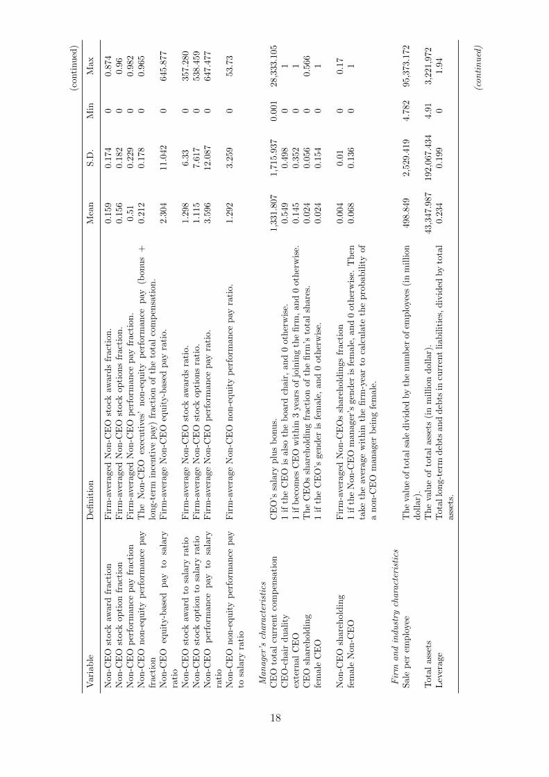
Table 2 reports definitions and summary statistics of our variables. The primary

focus is on managers’ Equity Fraction and Equity Ratio, and workers’ wages. First,

the incentive measure of most interest is the equity-based pay (stock award and stock

option) fractions (divided by total compensation) and ratios (divided by salary) for CEOs

and non-CEOs. We find that the magnitudes are substantial, and non-CEOs generally

have less incentive compensation than CEOs but not far behind. On average, Equity

Fraction is 36.7% for CEOs, and 29.8% for non-CEOs. Equity Ratio is 3.26 for CEOs

and 2.3 for non-CEOs. Next, aside from the equity, non-equity performance pay is

also important. For CEO, the non-equity performance pay constitutes 22.7% of CEOs’

15

total compensations, and 21.2% for non-CEOs. Measured against salary, the non-equity

performance pay to salary ratio is 1.69 for CEOs and 1.29 for non-CEOs. In terms of the

CEO’s controlling power of the firm, on average the probability of a CEO also serving as

the board chair is 54.9%.19 On average, the CEO owns 2.4% of the firm’s total shares.

Finally, the average yearly wage is 83,749 dollars, which include various benefits and

incentive pays to employees, with a large standard deviation, 66,509 dollars (in 2010

value).20

Table 1: Distributions of firms across major industries (%), the firm-level sample

Sector (1-digit SIC, division) Firms Employments

Mining and Construction 1.52 1.37Manufacturing 1: Food, Textile, Chemicals, etc. 8.28 7.23Manufacturing 2: Rubber, Machinery, Electronics, etc. 5.52 16.27Transportation, Communications, Electric, etc. 19.29 21.51Wholesale Trade & Retail Trade 8.75 17.84Finance, Insurance, and Real Estate 44.27 21.37Services 1: Hotel, Personal Business, Motion Picture, etc. 5.47 4.88Services 2: Health, Legal, Education, Social, etc. 6.9 9.54

19 The U.S. has a particularly high probability of CEO-chair duality comparing to other countries.It is declining in the recent decades thanks to the shareholder movements, including working-classshareholders (Webber 2018: 112-113).

20 In our sample, low-average wage (< 25 thousand dollars) and normal/high-wage observations co-exist in many industries, but Eating And Drinking Places industry (SIC 58) contains about 70% ofall low-wage observations and no high-wage observation. Nonetheless, our results remain intact whendropping all the SIC-58 observations, and we consistently control for industry-fixed effects throughoutanalyses.

16

Tab

le2:

Vari

ab

les

Defi

nit

ion

san

dS

um

mary

Sta

tist

ics,

Fir

m-L

evel

Sam

ple

Var

iab

leD

efin

itio

nM

ean

S.D

.M

inM

ax

Man

ager

an

dF

irm

Ch

ara

cter

isti

csat

the

firm

-yea

rle

vel

.(N

=5,5

79)

Wag

eY

earl

yto

tal

lab

or

an

dre

late

dex

pen

ses

(in

clu

din

gin

centi

vep

ays,

ben

efit

pla

ns,

pay

roll

taxes

,p

ensi

on

cost

s,p

rofi

tsh

ari

ng,

sala

ries

an

dw

ages

,an

dem

plo

yer

’sco

ntr

ibu

tion

toh

ealt

hin

sura

nce

),su

btr

act

edby

exec

uti

veco

mp

ensa

tion

,d

ivid

edby

the

tota

lnu

mb

erof

emp

loye

es(i

n20

10ye

ar

thou

san

dd

oll

ar)

.

83.7

49

66.5

06

2.9

21

741.0

2

Log

(yea

rly

wag

e)Y

earl

yw

age

inlo

gari

thm

s.4.1

79

0.7

42

1.0

72

6.6

08

Man

age

r’s

com

pen

sati

on

stru

ctu

reC

EO

equ

ity-b

ase

dp

ayfr

acti

onT

he

CE

O’s

equ

ity-b

ase

dp

ay(s

tock

award

s+

stock

op

tion

s)fr

act

ion

ofth

eto

tal

com

pen

sati

on

.0.3

67

0.2

59

01

CE

Ost

ock

awar

dfr

acti

onT

he

CE

O’s

stock

award

sfr

act

ion

of

the

tota

lco

mp

ensa

tion

.0.1

86

0.2

21

01

CE

Ost

ock

opti

onfr

acti

onT

he

CE

O’s

stock

op

tion

fract

ion

of

the

tota

lco

mp

ensa

tion

.0.1

81

0.2

25

00.9

71

CE

Op

erfo

rman

cep

ayfr

acti

onC

EO

’sb

onu

s+

lon

g-t

erm

ince

nti

vepay

+eq

uit

y-b

ase

dp

ay,ti

ll2005;

CE

O’s

non

-equit

yin

centi

ve

pay

+eq

uit

y-b

ase

dp

ay,

sin

ce2006.

Di-

vid

edby

the

tota

lco

mp

ensa

tion

.

0.5

83

0.2

70

1

CE

On

on-e

qu

ity

per

form

ance

pay

frac

-ti

onT

he

CE

O’s

non

-equ

ity

per

form

an

cep

ay(b

onu

s+

lon

g-t

erm

ince

nti

vep

ayti

ll20

05,n

on

-equ

ity

ince

nti

vep

aysi

nce

2006)

fract

ion

ofth

eto

tal

com

pen

sati

on

.

0.2

17

0.2

00.9

84

CE

Oeq

uit

y-b

ased

pay

tosa

lary

rati

oT

he

CE

O’s

equ

ity-b

ase

dp

ay(s

tock

award

s+

stock

opti

on

s)d

ivid

edby

sala

ry.

3.2

59

5.9

59

099.7

87

CE

Ost

ock

awar

dto

sala

ryra

tio

Th

eC

EO

’sst

ock

award

sd

ivid

edby

sala

ry.

1.6

99

4.0

64

095.4

CE

Ost

ock

opti

onto

sala

ryra

tio

Th

eC

EO

’sst

ock

op

tion

sd

ivid

edby

sala

ry.

1.5

60

3.9

21

084.7

36

CE

Op

erfo

rman

cep

ayto

sala

ryra

tio

CE

O’s

bon

us

+lo

ng-t

erm

ince

nti

vep

ay+

equ

ity-b

ase

dp

ay,ti

ll2005;

CE

O’s

non

-equit

yin

centi

ve

pay

+eq

uit

y-b

ase

dp

ay,

sin

ce2006.

Di-

vid

edby

sala

ry.

4.9

58.5

55

0156.1

65

CE

On

on-e

qu

ity

per

form

ance

pay

tosa

lary

rati

oT

he

CE

O’s

non

-equ

ity

per

form

an

cep

ay(b

onu

s+

lon

g-t

erm

ince

nti

vep

ayti

ll20

05,

non

-equ

ity

ince

nti

vep

aysi

nce

2006)

div

ided

by

sala

ry.

1.6

91

4.3

09

071.4

29

Non

-CE

Oeq

uit

y-b

ased

pay

frac

tion

Fir

m-a

ver

aged

Non

-CE

Oeq

uit

y-b

ase

dp

ayfr

act

ion

.0.2

98

0.1

92

00.9

05

(con

tin

ued

)

17

(conti

nu

ed)

Var

iab

leD

efin

itio

nM

ean

S.D

.M

inM

ax

Non

-CE

Ost

ock

awar

dfr

acti

onF

irm

-aver

aged

Non

-CE

Ost

ock

award

sfr

act

ion

.0.1

59

0.1

74

00.8

74

Non

-CE

Ost

ock

opti

onfr

acti

onF

irm

-ave

raged

Non

-CE

Ost

ock

op

tion

sfr

act

ion

.0.1

56

0.1

82

00.9

6N

on-C

EO

per

form

ance

pay

frac

tion

Fir

m-a

ver

aged

Non

-CE

Op

erfo

rman

cep

ayfr

act

ion

.0.5

10.2

29

00.9

82

Non

-CE

On

on-e

qu

ity

per

form

ance

pay

frac

tion

Th

eN

on-C

EO

exec

uti

ves

’n

on

-equ

ity

per

form

an

cep

ay(b

onu

s+

lon

g-te

rmin

centi

vep

ay)

fract

ion

of

the

tota

lco

mp

ensa

tion

.0.2

12

0.1

78

00.9

65

Non

-CE

Oeq

uit

y-b

ased

pay

tosa

lary

rati

oF

irm

-ave

rage

Non

-CE

Oeq

uit

y-b

ase

dp

ayra

tio.

2.3

04

11.0

42

0645.8

77

Non

-CE

Ost

ock

awar

dto

sala

ryra

tio

Fir

m-a

ver

age

Non

-CE

Ost

ock

award

sra

tio.

1.2

98

6.3

30

357.2

80

Non

-CE

Ost

ock

opti

onto

sala

ryra

tio

Fir

m-a

vera

ge

Non

-CE

Ost

ock

op

tion

sra

tio.

1.1

15

7.6

17

0538.4

59

Non

-CE

Op

erfo

rman

cep

ayto

sala

ryra

tio

Fir

m-a

vera

ge

Non

-CE

Op

erfo

rman

cep

ayra

tio.

3.5

96

12.0

87

0647.4

77

Non

-CE

On

on-e

qu

ity

per

form

ance

pay

tosa

lary

rati

oF

irm

-ave

rage

Non

-CE

On

on

-equ

ity

per

form

an

cep

ayra

tio.

1.2

92

3.2

59

053.7

3

Man

age

r’s

chara

cter

isti

csC

EO

tota

lcu

rren

tco

mp

ensa

tion

CE

O’s

sala

ryp

lus

bonu

s.1,3

31.8

07

1,7

15.9

37

0.0

01

28,3

33.1

05

CE

O-c

hai

rd

ual

ity

1if

the

CE

Ois

als

oth

eb

oard

chair

,an

d0

oth

erw

ise.

0.5

49

0.4

98

01

exte

rnal

CE

O1

ifb

ecom

esC

EO

wit

hin

3ye

ars

of

join

ing

the

firm

,an

d0

oth

erw

ise.

0.1

45

0.3

52

01

CE

Osh

areh

old

ing

Th

eC

EO

ssh

are

hold

ing

fract

ion

of

the

firm

’sto

tal

share

s.0.0

24

0.0

56

00.5

66

fem

ale

CE

O1

ifth

eC

EO

’sgen

der

isfe

male

,an

d0

oth

erw

ise.

0.0

24

0.1

54

01

Non

-CE

Osh

areh

old

ing

Fir

m-a

vera

ged

Non

-CE

Os

share

hold

ings

fract

ion

0.0

04

0.0

10

0.1

7fe

mal

eN

on-C

EO

1if

the

Non

-CE

Om

an

ager

’sgen

der

isfe

male

,an

d0

oth

erw

ise.

Th

enta

keth

eav

erage

wit

hin

the

firm

-yea

rto

calc

ula

teth

ep

rob

ab

ilit

yof

an

on-C

EO

man

ager

bei

ng

fem

ale

.

0.0

68

0.1

36

01

Fir

man

din

du

stry

chara

cter

isti

csS

ale

per

emplo

yee

Th

eva

lue

ofto

talsa

led

ivid

edby

the

nu

mb

erof

emp

loye

es(i

nm

illi

on

dol

lar)

.498.8

49

2,5

29.4

19

4.7

82

95,3

73.1

72

Tot

alas

sets

Th

eva

lue

ofto

tal

ass

ets

(in

mil

lion

doll

ar)

.43,3

47.9

87

192,0

67.4

34

4.9

13,2

21,9

72

Lev

erag

eT

otal

lon

g-te

rmd

ebts

an

dd

ebts

incu

rren

tli

ab

ilit

ies,

div

ided

by

tota

las

sets

.0.2

34

0.1

99

01.9

4

(con

tin

ued

)

18

(conti

nu

ed)

Var

iab

leD

efin

itio

nM

ean

S.D

.M

inM

ax

For

eign

Act

ivit

y1

ifth

efi

rmre

ceiv

esany

fore

ign

inco

mes

or

pay

sfo

reig

nta

xes

,0

oth

erw

ise.

0.3

57

0.4

79

01

Cap

ital

exp

end

itu

res

by

asse

tsT

he

fun

ds

use

dfo

rad

dit

ion

sto

pro

per

ty,

pla

nt,

an

deq

uip

men

t,ex

-cl

ud

ing

amou

nts

ari

sin

gfr

om

acq

uis

itio

ns,

div

ided

by

tota

lass

ets.

InM

illi

ons

ofd

ollars

.

0.0

47

0.0

62

-0.0

01

0.5

97

Fir

m-s

pec

ific

tim

etr

end

sT

he

year

ssi

nce

the

firm

firs

tap

pea

rsin

the

Com

pu

stat

data

base

(197

0-20

16).

18.8

51

11.2

47

147

HH

IT

he

Her

fin

dah

l-H

irsc

hm

an

ind

exat

the

2-d

igit

SIC

-yea

rle

vel,

base

don

Com

pu

stat

data

set.

Ah

igh

erH

HI

ind

icate

sa

hig

her

deg

ree

of

sale

con

centr

ati

on

inth

ein

du

stry

.

882.9

02

611.2

82

76.9

18

6,1

85.7

5

Wor

kers

’ch

ara

cter

isti

csat

the

2-d

igit

SIC

-yea

rle

vel

(N=

776)

Pro

por

tion

Age

10.1

36

0.1

08

00.5

97

Pro

por

tion

Age

20.2

51

0.0

55

0.0

87

0.4

75

Pro

por

tion

Age

30.2

63

0.0

58

0.0

98

0.4

41

Pro

por

tion

Age

40.2

23

0.0

66

0.0

42

0.4

72

Pro

por

tion

Age

50.1

09

0.0

46

0.0

04

0.3

14

Pro

por

tion

Age

60.0

19

0.0

16

00.1

03

Pro

por

tion

Fem

ale

1if

the

wor

ker

’sgen

der

isfe

male

,0

oth

erw

ise.

0.3

74

0.1

82

0.0

10.8

07

Pro

por

tion

Yea

rsof

edu

cati

on9

1if

hig

hes

tle

vel

of

edu

cati

on

is9th

deg

ree

(≤9

yea

rs),

0oth

erw

ise

0.0

34

0.0

33

00.1

73

Pro

por

tion

Yea

rsof

edu

cati

on10

1if

hig

hes

tle

vel

of

edu

cati

on

is10th

gra

de,

0oth

erw

ise

0.0

18

0.0

18

00.1

12

Pro

por

tion

Yea

rsof

edu

cati

on11

1if

hig

hes

tle

vel

of

edu

cati

on

is11th

gra

de,

0oth

erw

ise

0.0

35

0.0

29

00.1

61

Pro

por

tion

Yea

rsof

edu

cati

on12

1if

hig

hes

tle

vel

of

edu

cati

on

is12th

gra

de/

hig

hsc

hool

gra

du

ate

,0

oth

erw

ise

0.3

20.1

09

0.0

67

0.6

22

Pro

por

tion

Yea

rsof

edu

cati

on13

1if

hig

hes

tle

vel

of

edu

cati

on

isso

me

coll

ege,

0oth

erw

ise

0.2

02

0.0

47

0.0

67

0.3

75

Pro

por

tion

Yea

rsof

edu

cati

on14

1if

hig

hes

tle

vel

of

edu

cati

on

isass

oci

ate

deg

ree,

0oth

erw

ise

0.0

94

0.0

34

0.0

28

0.2

2P

rop

orti

onY

ears

ofed

uca

tion

161

ifh

igh

est

level

of

edu

cati

on

isb

ach

elor’

sd

egre

e,0

oth

erw

ise

0.2

19

0.1

09

0.0

29

0.5

84

Pro

por

tion

Yea

rsof

edu

cati

on18

1if

hig

hes

tle

vel

of

edu

cati

on

ism

ast

er’s

deg

ree,

0oth

erw

ise

0.0

63

0.0

50

0.2

42

Pro

por

tion

Yea

rsof

edu

cati

on19

1if

hig

hes

tle

vel

of

edu

cati

on

isp

rofe

ssio

nal

deg

ree,

0oth

erw

ise

0.0

07

0.0

08

00.0

43

Pro

por

tion

Yea

rsof

edu

cati

on23

1if

hig

hes

tle

vel

of

edu

cati

on

isd

oct

ora

ted

egre

e,0

oth

erw

ise

0.0

09

0.0

14

00.1

04

Pro

por

tion

Exp

erie

nce

10.2

60.1

18

0.0

34

0.7

04

Pro

por

tion

Exp

erie

nce

20.2

56

0.0

51

0.1

07

0.4

19

(con

tin

ued

)

19

(conti

nu

ed)

Var

iab

leD

efin

itio

nM

ean

S.D

.M

inM

ax

Pro

por

tion

Exp

erie

nce

30.2

48

0.0

60.0

72

0.4

72

Pro

por

tion

Exp

erie

nce

40.1

74

0.0

66

0.0

20.4

34

Pro

por

tion

Exp

erie

nce

50.0

62

0.0

31

00.2

09

Par

t-ti

me

Full

/par

t-ti

me

statu

s,1

ifth

ew

ork

eris

ap

art

-tim

ew

ork

er,

0oth

er-

wis

e.0.1

0.1

12

00.4

99

Non

-wh

ite

race

1if

the

wor

ker’

sra

ceis

non

-wh

ite,

0oth

erw

ise.

0.1

84

0.0

57

0.0

23

0.4

56

Pro

por

tion

Un

ion

cover

age

1if

cove

red

by

un

ion

or

coll

ecti

veagre

emen

t,0

oth

erw

ise.

0.1

65

0.1

66

00.8

59

Pro

por

tion

Urb

anre

sid

ence

11

ifn

otid

enti

fiab

leor

not

inm

etro

are

a;

0.1

52

0.1

16

0.0

10.6

9P

rop

orti

onU

rban

resi

den

ce2

1if

centr

alci

ty,

0oth

erw

ise

0.2

49

0.0

79

00.5

23

Pro

por

tion

Urb

anre

sid

ence

31

ifou

tsid

ece

ntr

al

city

,0

oth

erw

ise

0.4

58

0.0

87

0.1

48

0.6

74

Pro

por

tion

Urb

anre

sid

ence

41

ifce

ntr

alci

tyst

atu

su

nkn

own

,0

oth

erw

ise

0.1

34

0.0

37

0.0

32

0.3

14

Pro

por

tion

Mar

ital

stat

us

11

ifm

arri

ed,

spou

sep

rese

nt,

0oth

erw

ise

0.5

82

0.1

10.1

98

0.8

6P

rop

orti

onM

arit

alst

atu

s2

1if

mar

ried

,sp

ou

seab

sent,

0oth

erw

ise

0.0

12

0.0

08

00.0

69

Pro

por

tion

Mar

ital

stat

us

31

ifse

par

ated

,0

oth

erw

ise

0.0

23

0.0

12

00.0

9P

rop

orti

onM

arit

alst

atu

s4

1if

div

orce

d,

0oth

erw

ise

0.1

08

0.0

27

0.0

10.1

92

Pro

por

tion

Mar

ital

stat

us

51

ifw

idow

ed,

0oth

erw

ise

0.0

14

0.0

09

00.0

92

Pro

por

tion

Mar

ital

stat

us

61

ifn

ever

marr

ied

/si

ngle

,0

oth

erw

ise

0.2

61

0.1

14

0.0

42

0.6

95

20

3.1.5 Model Specification

We estimate a standard fixed effect model as follows:

log(wkjsct) = αkjsct + βXkjst + γMkjst + δIkjst + φVjt + µFjsct + εkjsct, (14)

where w is the yearly total wage, so log(wkjst) is the log wage of firm k in industry j

in state s and incorporation state c at year t. The firm-fixed effects are included in

αkjsct. Xkjsct denotes managerial compensation structures including Equity Fraction,

Equity Ratio, etc. Mkjst includes other manager characteristics and three variables of

managerial controlling power. Ikjst includes firm characteristics, and Vjt includes ten

workers’ characteristics at the industry level. Fjsct are industry-, state-, year-, and

incorporation-state-year fixed effects, and HHI by industry-year. The robust standard

errors are clustered at the firm level. The estimations of β is of particular interest in the

following analyses.

3.2 Results from basic correlation analyses

Table 3 reports basic results of estimation. Consistent with the theoretical prediction,

column (1) and (2) show that all else equal, an increase in CEO Equity Fraction by one

standard deviation (25.9%) is associated with 1.5% lower wages. An increase in Equity

Ratio is also negatively associated with wages, although not statistically significant at

the 10% level. The effect of non-CEO Equity Fraction in column (3) is stronger than

the result of CEO Equity Fraction, while the effect of non-CEO Equity Ratio (column

(4)) is also weaker and statistically insignificant.

Next, we decompose the equity-based pays into stock awards and stock options to

check whether their effects on wages are the same. In Table 4, column (1) and (2)

show the effects of Stock Fraction (stock awards divided by the total compensation) and

Option Fraction (Stock options divided by the total compensation), while column (5)

and (6)shows the effects of Stock Ratio (stock awards divided by salary) and Option Ratio

(stock options divided by salary). Except Stock Ratio which is statistically insignificant,

the coefficients of all other three measures show clear negative effects on wages. These

findings strengthen the theoretical prediction that more equity-based pay, be it stock or

option, correlates with lower wages.

We further test the effects of the performance pay as a whole, and the effects of

non-equity performance pay in particular. The results of column (3) and (7) show that

performance pay as a whole tends to have negative effects on wages. This is not surprising

given the fact that most of the performance pays are equity-based. In contrast, while

21

also being parts of the performance pay, the results of column (4) and (8) show that

non-equity elements have positive effects on wages. This interesting result appears again

in our robustness tests based on an individual-level sample in Section 3.3.3.

Table 3: Effects of Equity-Fraction and Equity-Ratio on Wages, Baseline Results

Dependent Variable: Log(Yearly Average Wage)(1) (2) (3) (4)

CEO equity-based pay fraction -0.058***(0.021)

CEO equity/salary ratio -0.002(0.001)

Non-CEO equity-based pay fraction -0.114***(0.034)

Non-CEO equity/salary ratio -0.001(0.001)

Manager characteristics by firm-year Yes Yes Yes YesFirm characteristics by firm-year Yes Yes Yes YesWorker characteristics by industry-year Yes Yes Yes YesHHI by industry-year Yes Yes Yes YesFirm-, industry-, state-, and year-fixedeffects

Yes Yes Yes Yes

Incorporation state-year-fixed effects Yes Yes Yes Yes

R-squared 0.307 0.305 0.309 0.304Observations 5,579 5,579 5,579 5,579Number of firms 651 651 651 651

Robust standard errors in parentheses: *** p<0.01, ** p<0.05, * p<0.1

Notes. Equity based pay fraction is defined as the fraction of stock award and stock option in the executive totalcompensation. Equity/salary ratio is defined as the value of stock award plus stock option divided by the value of salary.Manager characteristics include: gender, total amount of current compensations (salary + bonus), CEO-chair duality,externally-hired CEO, non-CEO’s gender. Firm characteristics includes: foreign activity dummy, sales per employee,total assets, leverage ratio, capital expenditure divided by total assets, and firm’s age. Worker characteristics include:gender, race, age, education, experience, union coverage, full/part-time status, urban residence, and marital status, allcalculated as proportions at the 2-SIC digit-year level. Robust standard errors are adjusted for clustering at the firmlevel.

22

Table 4: Effects of Four Components of Compensation, Firm-Level Sample

Dependent Variable: Log(Yearly Wage)(1) (2) (3) (4) (5) (6) (7) (8)

CEO stock award fraction -0.044*(0.027)

CEO stock option fraction -0.045*(0.024)

CEO performance pay -0.036fraction (0.023)CEO non-equity perf. pay 0.051**fraction (0.025)

CEO stocks award ratio 0.000(0.002)

CEO stock options ratio -0.003**(0.002)

CEO performance pay -0.001ratio (0.001)CEO non-equity perf. pay 0.003

(0.002)

Managers’ characteristicsby firm-year

Yes Yes Yes Yes Yes Yes Yes Yes

Worker characteristics byindustry-year

Yes Yes Yes Yes Yes Yes Yes Yes

Firm characteristics byfirm-year

Yes Yes Yes Yes Yes Yes Yes Yes

HHI by industry-year Yes Yes Yes Yes Yes Yes Yes YesFirm-, industry-, state-,and year-fixed effects

Yes Yes Yes Yes Yes Yes Yes Yes

Incorporation state-year-fixed effect

Yes Yes Yes Yes Yes Yes Yes Yes

R-squared 0.305 0.305 0.305 0.305 0.304 0.306 0.304 0.305Observations 5,579 5,579 5,579 5,579 5,579 5,579 5,579 5,579Number of firms 651 651 651 651 651 651 651 651

Robust standard errors in parentheses: *** p<0.01, ** p<0.05, * p<0.1

Notes. Performance pay fraction is defined as the fraction of bonus + long-term incentive pay + equity-based pay, till2005; CEO’s non-equity incentive pay + equity-based pay, since 2006, in the executive total compensation. Stock awardand stock option fractions are defined as the value of stock award and stock option divided by the value of the executivetotal compensation. Stock award/salary ratio and stock option/salary ratio are defined as the value of stock award andstock option divided by the value of salary. Non-equity performance pay fraction is defined as the fraction of bonus +long-term incentive pay till 2005, non-equity incentive pay since 2006, in the executive total compensation. Managercharacteristics include: gender, total amount of current compensations (salary + bonus), CEO-chair duality,externally-hired CEO, non-CEO’s gender. Firm characteristics includes: foreign activity dummy, sales per employee,total assets, leverage ratio, capital expenditure divided by total assets, and firm’s age. Worker characteristics include:gender, race, age, education, experience, union coverage, full/part-time status, urban residence, and marital status, allcalculated as proportions at the 2-SIC digit-year level. Robust standard errors are adjusted for clustering at the firmlevel.

3.3 Robustness tests

To address several potential concerns regarding our baseline results based on the firm-

level sample, in this section we report results from a set of robustness tests. First, a

sample selection bias may occur because only about 20% of the firms in Compustat report

labor expenses. To deal with this concern, we estimate the Heckman bias correction

model and find similar results (Section 3.3.1). We further estimate the same model

using the individual-level sample which does not suffer from the problem, and still find

23

consistent results (Section 3.3.3).21

Second, we examine if our baseline results are biased due to the over-representation

of financial firms in the firm-level sample, or omitting the industry-year specific shocks.

The results suggest that our baseline results are reliable. The literature on managerial

incentives typically focuses on the managerial shareholding. We find that controlling for

managerial shareholdings does not change our baseline results (Section 3.3.2).

Third, another concern is composition changes, which refers to the problem that,

due to business offshoring, the labor expenses reported by firms include wages paid to

employees hired in foreign countries. If the wages of the foreign employees are different

from the ones in the U.S., a lower mean wage of the firm may reflect either a composition

change, a true wage reduction for all workers, or a mix of both. My analyses based on the

individual-level sample which includes only workers in the U.S., verify that the negative

effects remain statistically significant (Section 3.3.3).

3.3.1 Sample selection bias

Because firms have not been required to disclose workers’ wages under the U.S. Generally

Accepted Accounting Principles (GAAP) until very recently,22 only about 20% of firms

have reported wages, and they tend to be larger and concentrate in especially the financial

sector, as shown in Table 1. This raises a concern of sample selection bias.

To address the concern of selection bias, we estimate Heckman’s (1976) two-step

correction model and report the results in Appendix 3, Table 7. Following the approach

of Shin (2014), we estimate a series of probit models to identify variables that predict

the probability of reporting labor cost, and then find out which ones do not affect the

wage level by running a set of regressions with all explanatory variables. The diagnostics

suggest that firms reporting selling, general, and administrative expenses (Compustat

item: xsga) are unlikely to disclose labor costs due to some accounting practices that are

unrelated to the wage level. Therefore we use a binary variable indicating whether the

firm reports selling, general, and administrative expenses as the selection variable in the

Heckman models. As shown in Table 7 (Appendix 3), the results from Heckman models

are similar with the baseline results in Table 3 and confirm the negative correlation

between managerial equity-based pay and workers’ wages.

21 These results are consistent with recent studies using the same average wage data based on Com-pustat, such as Chemmanur, Cheng, & Zhang (2013) and Faleye, Reis & Venkateswaran (2013).

22 With the implementation of the Dodd-Frank Wall Street Reform and Consumer Protection Act,U.S. firms will need to disclose the median employee compensation, the CEO’s compensation, and theratio of the two, starting at 2018.

24

3.3.2 Non-finance vs. finance, industry-year-fixed effects, and managerialshareholding

We further perform two other robustness tests and report the results in Appendix 4.

First, since about 44% of the firms in the sample concentrate in the financial sector, there

is a concern whether the heterogeneity across different industries biases the estimation.

We divide the sample into non-financial and financial sectors and estimate the same

model. As shown in Appendix 4 Table 8 from Column (1) to (4), non-financial firms

show the same effects as the whole sample. Although the statistical significance of the

CEO Equity Fraction or Equity Ratio in financial sector is weaker, the results are still

consistent and show negative associations of equity-based pay on wages.

Second, it’s possible that a temporary shock specific to one industry-year may lead

the firms of the industry-year to increase executive equity-based pays and hire more

temporary, low-wage workers. To address this issue, we add industry-year-fixed effects

in to the model to control for potential shocks specific to an industry-year. As shown

in Appendix 4 Table 8 Column (5) and (6), the results remain similar with our baseline

results.

Third, to compare with the literature that focus on the effect of managerial share-

holding, we include the CEO’s shareholding fraction in controlling variables, measured

by the percentage of the firm’s stocks owned by the CEO. As shown in Appendix 4

Table 8 Column (7) and (8), controlling for managerial shareholding does not change

our baseline results.

3.3.3 Sample selection bias, and composition changes by offshoring: testsusing the individual-level sample

A concern of the firm-level sample is that a lower mean wage of the firm may reflect

firms’ offshorings to low-wage countries rather than direct wage reductions. One way

to address this concern is to construct a sample containing only workers in the U.S.

economy for analysis. We use individual U.S. workers’ data (CPS) who are hired in big

firms (employing 500 workers and more), and then match them with CEO’s compensa-

tion structure and firms’ information, also limiting to big firms, calculated at the 2-digit

industry level.23 This produces a multi-year, cross-sectional data set with the basic unit

being an U.S. worker. Compared to the firm-level sample in which we have individual

23 Since CPS contains significant amount of employees who work in small firms, while the Compustatand Execucomp data tend to be reported by big firms, we require individual workers, firms, and managersin the matched data set all to be in big firms, defined as a firm hired at least 500 employees. In thisway although we can’t link individual workers precisely to their firms, and many workers not employedin the firms in the Compustat-Execucomp linked database are inevitably included in, the workers in thesample should overlap largely with our targeted firms’ employees.

25

firms’ and managers’ information with workers’ characteristics at the industry level, here

we have an individual worker-level sample with firms’ and managers’ characteristics at

the industry level. Since the information of firm and manager covered in this sample

is not constrained by whether the firm reports labor expenses, this sample is compre-

hensive and does not suffer from the concern of sample selection bias. Details of the

sample, summary statistics, model specification, and the regression tables are reported

in Appendix 5.

With the individual-level sample, we estimate a cross-section model in which the log

hourly wage of individual workers is the dependent variable, and the industry-level CEO

Equity Fraction or Equity Ratio, is the explanatory variable, controlling for a rich set of

individual-level characteristics including occupation which is not feasible in the firm-level

sample. We further test whether the results vary with two different measures of wages:

one includes and the other excludes the amount of employer’s contribution for health

insurance, since the accuracy of reports of the contributions may be a concern.

Across these settings, results from this individual-level sample are similar with our

baseline results. As shown in Appendix 5 Table 11 column (1) and (2), the effects of the

equity-based pay on wages are all negative and statistically significant. All else equal, an

increase in CEO Equity Fraction by one standard deviation (12.4%) is associated with

0.46% lower wages, and an inrease in CEO Eqyuity Ratio by one standrad deviation

(3.959) is associated with 0.15% lower wages. Column (3) and (4) show that the results

are not affected if we exclude the employer’s contribution for health insurance from the

measure of wage. These results are consistent with the theoretical prediction, and verify

that at least parts of the negative effects of equity-based pays on wages in previous

sections are not driven by offshorings. They also suggest that the concern of sample

selection bias may not be too serious.

Next, as in the analyses of the firm-level sample, We decompose the equity-based

pay into stocks and options, and also compute variables for performance pay and non-

equity performance pay. As shown in Table 12, the directions of the coefficients of most

variables are the same as in the firm-level analyses (Table 4), although the magnitudes

are smaller. On the one hand, more stock awards and stock options also associate with

lower wages, and so do performance pay, consisting with our theoretical prediction. On

the other hand, non-equity performance pay associates with higher wages both in the

firm-level and the individual-level samples. This interesting result, however, should be

treated with caution, because there is no clear theory to rigorously guide our estimation

and prediction, and the designs of non-equity performance pay (bonuses and long-term

incentives) are likely to be more complex and diverse among firms than equity-based

26

pays.

4 Identification Strategy

The analyses in the previous sections show that workers’ wages are lower as managers

receive more equity-based pays. However, the correlation may not mean causality. There

might be unobserved factors, such as a technology change and a worrisome business out-

look, affecting both managers’ compensation structures and workers’ wages and creating

the negative correlation we saw in Section 3. To test whether the effect is causal or not,

we need to identify a change in the managerial compensation structure that is unrelated

to these unobserved factors. In this section, we utilize a change in the corporate tax

policy as an instrumental variable for the CEO’s compensation structure and implement

the IV estimation. Section 4.1 explains the institutional background and the choice of

my instrumental variable. Section 4.2 presents the model specification and estimation

results.

4.1 Internal Revenue Code 162(m) and the construction of IV

Enacted by Congress in 1993, section 162(m) of the Internal Revenue Code limits the de-

ductibility of top five executives’ non-performance-related compensations over $1 million,

and imposes a 60% federal surtax on salaries above $1 million. In this way, the legislation

encourages firms to increase the use of performance pay rather than fixed salary while

leaving open the total amounts of compensations. Responding to the legislation, several

studies found that firms originally paying higher salaries reduce salaries to $1 million,

and firms originally paying lower raise salaries over time but don’t go above $1 million

(Perry & Zenner, 2001; Rose & Wolfram, 2002). At the same time, the growth of the

total amounts of executive compensation has been unaffected by the legislation. Firms

simply switched from salary to other forms of compensations such that the structure

of executive compensation has became more equity-based and more sensitive to firms’

(stock market) performances (Perry & Zenner, 2001; Balsam & Ryan, 2007).

As shown in Figure 1, in my firm-level sample there is indeed a significant, abnormal

bunch of firms paying CEOs’ salaries right at the tax deductibility threshold, one million

dollars. Further, in Figure 2, by graphing the distribution separately in every five-years

period, we can see clearly that this bunch grows higher and higher over each period. This

implies that many firms indeed are affected by legislation and freeze CEOs’ salaries at

the threshold, and the amount of firms affected grows over time. In this case, if the firms

want to pay their CEOs more, they are more likely raise performance pay especially the

27

equity-based pay, and we will see a change in the compensation structure as a result.

Figure 1: The bunching distribution of firms by CEO’s salary, whole-sample period(1992-2016)

28

Figure 2: The bunching distribution of firms by CEO’s salary, five-year periods

A few issues need to be dealt with before we can utilize the legislation as an instru-

ment for estimation. First, the choice of measurement. The key compensation item this

legislation aimed to limit is salary, so the effect of the legislation on compensation struc-

ture would be captured more precisely by a measurement of equity-based pay relative

to salary, rather than the shareholding as commonly used in the literature. Two mea-

surements of CEO equity-based compensation, Equity-Fraction and Equity-Ratio, are

used in the previous analyses. The former is expected to be too noisy in measuring and

interpreting the change, because it uses total compensation as the denominator which

includes salary, bonus, equity, non-equity incentives, etc, and many of them may also

change as equity increases, and the effects can be complex. Therefore, to capture the

policy change more precisely, a natural choice of measurement seems to be the equity-

based pay-to-salary ratio. To pin down the interpretation, we further focus on the CEO

in the following analyses but continue controlling for variables of non-CEO managers’

controlling powers.

Second, to analyze the causal effect, we need to identify the treatment imposed

on firms. While CEOs’ compensation structures may change, which firms were really

affected by the legislature is not completely clear. Intuitively, the treatment effect of

29

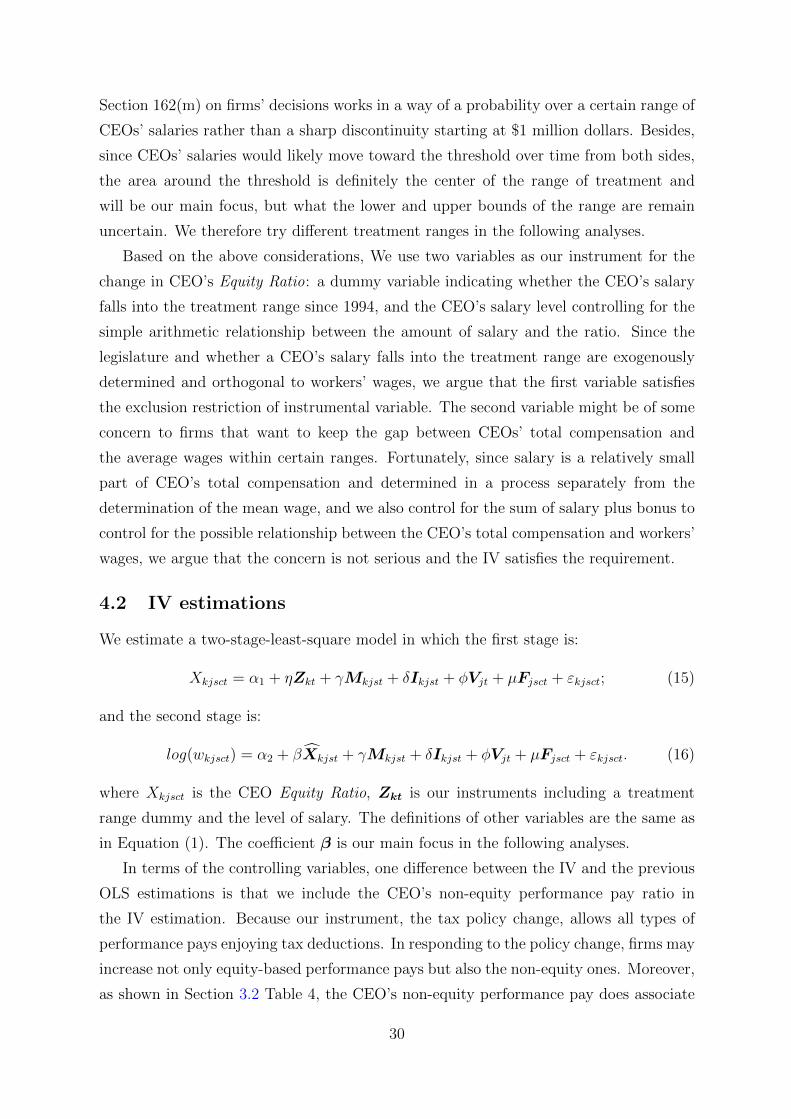
Section 162(m) on firms’ decisions works in a way of a probability over a certain range of

CEOs’ salaries rather than a sharp discontinuity starting at $1 million dollars. Besides,

since CEOs’ salaries would likely move toward the threshold over time from both sides,

the area around the threshold is definitely the center of the range of treatment and

will be our main focus, but what the lower and upper bounds of the range are remain

uncertain. We therefore try different treatment ranges in the following analyses.

Based on the above considerations, We use two variables as our instrument for the

change in CEO’s Equity Ratio: a dummy variable indicating whether the CEO’s salary

falls into the treatment range since 1994, and the CEO’s salary level controlling for the

simple arithmetic relationship between the amount of salary and the ratio. Since the

legislature and whether a CEO’s salary falls into the treatment range are exogenously

determined and orthogonal to workers’ wages, we argue that the first variable satisfies

the exclusion restriction of instrumental variable. The second variable might be of some

concern to firms that want to keep the gap between CEOs’ total compensation and

the average wages within certain ranges. Fortunately, since salary is a relatively small

part of CEO’s total compensation and determined in a process separately from the

determination of the mean wage, and we also control for the sum of salary plus bonus to

control for the possible relationship between the CEO’s total compensation and workers’

wages, we argue that the concern is not serious and the IV satisfies the requirement.

4.2 IV estimations

We estimate a two-stage-least-square model in which the first stage is:

Xkjsct = α1 + ηZkt + γMkjst + δIkjst + φVjt + µFjsct + εkjsct; (15)

and the second stage is:

log(wkjsct) = α2 + βXkjst + γMkjst + δIkjst + φVjt + µFjsct + εkjsct. (16)

where Xkjsct is the CEO Equity Ratio, Zkt is our instruments including a treatment

range dummy and the level of salary. The definitions of other variables are the same as

in Equation (1). The coefficient β is our main focus in the following analyses.

In terms of the controlling variables, one difference between the IV and the previous

OLS estimations is that we include the CEO’s non-equity performance pay ratio in

the IV estimation. Because our instrument, the tax policy change, allows all types of

performance pays enjoying tax deductions. In responding to the policy change, firms may

increase not only equity-based performance pays but also the non-equity ones. Moreover,

as shown in Section 3.2 Table 4, the CEO’s non-equity performance pay does associate

30

with higher wages. In this case, if we omit the non-equity performance pay, the effect

of out instrument on wages will likely go through this omitted variable, and violate the

exclusion restriction.24

Another difference is the control of firm-fixed effects (or CEO-fixed effects). While

we control for firm-fixed effects in previous estimations, doing so will understandably

invalidate the instrument, particularly the treatment range dummy, since firms do not

switch in and out of the treatment frequently, there is not enough variation of the

treatment within firms. In spite of this limitation, we had compared the CEO’s Equity

Ratio effects before and after controlling for the firm-fixed effects (using the model in

column (2) of Table 3), and found that the sign of the coefficients remains the same while

the magnitudes are very similar. This suggests that the concern of leaving out firm-fixed

effects would be moderate.

The results of IV estimation are reported in Table 5. Due to the uncertainty of the

treatment range of the legislation, columns (1) to (4) try various bounds of the treatment

range which all include the bunching center, $1 million dollars. For example, column (1)

shows the results from using a treatment range covering salaries starting at 750 thousand

dollars.

24 The results are very similar if we include non-equity performance pay in the baseline analyses.

31

Table 5: Evidence on Causality, IV Estimation (LIML Estimator)

Treatment range 750- 850- 950- 1000-($Salary, thousand dollars; year ≥ 1994) (1) (2) (3) (4)

First Stage Dependent Variable: CEO equity/salary ratio

Treatment range dummy 0.684** 0.886*** 0.936*** 0.536(0.314) (0.302) (0.323) (0.33)

Salary -0.002*** -0.002*** -0.002*** -0.002***(0.001) (0.001) (0.001) (0.001)

1st-stage F of IV 8.69 9.51 9.82 5MOP effective F 5.82 6.91 6.83 5.48

Second Stage Dependent Variable: Log(Yearly Average Wage)

CEO equity/salary ratio -0.047* -0.041* -0.039*(0.025) (0.022) (0.022)

CLR test p-value (H0: β = 0) 0.023 0.029CLR 95% conf. sets [-.111, -.006] [-.1, -.004]

Controlling VariablesManager characteristics by firm-year Yes Yes Yes YesFirm characteristics by firm-year Yes Yes Yes YesWorker characteristics by industry-year Yes Yes Yes YesHHI by industry-year Yes Yes Yes YesState-, industry-, and year-fixed effects Yes Yes Yes YesIncorporation state-year-fixed effects Yes Yes Yes Yes

Observations 5,579 5,579 5,579 5,579Number of firms 651 651 651 651

Robust S.E. in parentheses: *** p<0.01, ** p<0.05, * p<0.1. Clustered at firms.

Notes. Column (1) to (4) are results using treatment ranges of 750/850/950/1000 thousand dollars and above. Equitybased pay/salary ratio is defined as the value of stock award plus stock option divided by the value of salary. Managercharacteristics include: gender, total amount of current compensations (salary + bonus), CEO-chair duality,externally-hired CEO, non-CEO’s gender, the CEO’s and non-CEO’s non-equity performance pay ratios. Firmcharacteristics includes: foreign activity dummy, sales per employee, total assets, leverage ratio, capital expendituredivided by total assets, and firm’s age. Worker characteristics include: gender, race, age, education, experience, unioncoverage, full/part-time status, urban residence, and marital status, all calculated as proportions at the 2-SIC digit-yearlevel. All controlling variables are the same as in correlation analyses except the non-equity performance pay ratio andfirm-fixed effects. Robust standard errors are adjusted for clustering at the firm level. MOP effective F and CLR testp-value and confidence sets are reported following the recommendations by Andrews, Stock, and Sun (2018).

The results from the first stage estimation suggest that our instruments are valid in

general, and the directions are also consistent with our prediction, i.e., the IRC 162(m)

legislation increases the use of equity based pays. The results are robust across various

choices of treatment ranges as long as the area around the threshold is included. Other-

wise, as shown in column (4), the dummy variable of the treatment fails to capture the

variation of CEO equity/salary ratio at 10% statistically significant level. This is con-

sistent with the implication that the estimated results are driven by the policy-induced

change in the compensation structure around the threshold, rather than unobservable

factors varied with CEOs’ salaries.

32

The F- and Montiel Olea-Pflueger (MOP) effective F-statistics, however, are all

smaller than the rule-of-thumb value, 10, suggesting that our instruments are weak.

To deal with this issue, the results reported in Table 5 are based on the Limited In-

formation Maximum Likelihood (LIML) estimator25 which is more nearly centered at

the true value of the estimand (Stock & Watson, 2003: 467). In addition, we adopt

the weak-IV robust inference method suggested by Andrews, Stock & Sun (2018) and

report the results from Conditional Likelihood Ratio (CLR) tests using the treatment

ranges of 850- and 950-. As shown in the column (2) and (3) in Table 5, the p-values the

CLR tests suggest that we can reject the null hypothesis that true value of the estimand

is zero, and the confidence sets do not include zero or the non-IV estimates from our

baseline results (-0.002), implying that our estimation is still reliable in spite of weak

instruments.

Based on the results of the second stage estimation, our IV estimation largely agrees

with our baseline OLS estimation: given the validity of the instrumental variables, the

effect of CEO equity/salary ratio on wages is clearly negative, and the coefficients in

Column (2) and (3) are around -0.04 which are much stronger and significant compared

to the previous result in Table 3 column (2) (-0.002). This evidence therefore indicates

that one unit increase in the CEO’s equity-to-salary ratio, say, from 1:1 to 2:1, will lead

to about a 4% reduction in the average wage, all else equal. Put it in another way, an

increase in the CEO’s equity-to-salary ratio by one standard deviation (4.06) will lead

to 16.24% lower wages.

5 Whether and how is the effect of CEO equity Pay

on Wages affected by competition?

In previous analyses, we hold the degree of market competition constant by consistently

controlling for HHI. In this section, we move beyond the average results and analyze

whether and how is the effect of CEO equity pay on wages affected by different degrees

of market competition.26

25 The original 2SLS results are very similar.26 Please note that we keep focusing on the consequence of CEO compensation structure in this section,

rather than the cause of it. Regarding the later question, there is a large literature on the product marketcompetition effect on managerial incentive provisions, but the direction remains indeterminate. Forexample, theoretically, while Hart (1983) suggests competition reduces the managerial slacks implyingless need for managerial incentive provisions, Scharfstein (1988), Hermalin (1992), Schmidt (1997), andRaith (2003) argue that the effects vary with various conditions, and the results can be ambiguous.Empirically, Cunat & Guadalupe (2009) find that more competition increases managerial incentiveprovisions and the sensitivity of pay to performance, but Fernandes, Ferreira & Winters (2018) findopposite results. To investigate this question, one needs to identify an exogenous change in the degree

33

5.1 Theory

A theory argues that corporate governance doesn’t matter in competitive markets, be-

cause competition constantly forces managers to reduce any slack or waste for surviving,

with or without a good governance institution. Therefore, a change in the governance in-

stitution should make little difference for firms’ performances when competition is strong.

Supporting this theory, Giroud & Mueller (2010) show that an exogenous change in the

anti-takeover regulation, which makes managers less likely to be punished for shirking,

has no impact on performances when the degree of competition is at the high level,

comparing to when competition degree is low.

Does this apply to the negative impact of CEO equity pay on wages as well? We

suspect not. Regarding the relationship with competition, a key difference between other

governance institutions and compensation is: other governance institutions are designed

to replicate the discipline of competition particularly when competition is weak. Hence,

it’s quite natural that governance makes little difference when competition is strong.

In contrast, compensation is designed to translate market valuation into the manager’s

reward assuming that competition and market valuation work well. Therefore the effect

of compensation should be larger when competition is strong, but may not function well

when competition is weak.

More specifically, under strong competition, market valuation is more sensitive to the

change in firm performances, such that the same gap in performance can generate a larger

difference in stock prices, comparing to the case under weak competition. Since equity-

based compensation ties the manager’s reward to the stock price, a larger difference in

prices means a larger difference in the manager’s monetary income between keeping the

peaceful labor relation or choosing high-level monitoring and reducing wages. Therefore,

at any given equity ratio, the opportunity cost for the manager to keep the peaceful

labor relation is higher under strong competition than weak competition, such that the

manager will more likely choose high-level monitoring and reduce wages.

We can use the model presented in Section 2 to pin down the idea. In that model,

even under the assumption that a higher monitor level does not bring higher outputs

(y), because surplus (Π) is still affected by the manager’s choice of monitor level, the

manager may still be willing to exercise high-level monitoring and trade off the private

benefit from a peaceful life for equity income, as long as the equity ratio is high enough.

There, we implicitly assume that the sensitivity of stock price to surplus is identical

of competition, which is beyond the scope of this paper. In this section, we simply show that EquityRatio goes up with all three degrees of competition in our first-stage estimation, and then keep focusingon the marginal effects.

34

across industries, which may be more legitimate when analyzing the average pattern.

Now, if we are to analyze the possibly different impacts on wages under different degrees

of competition, we would let the price-to-surplus sensitivity vary with the degree of

competition. In addition, we would expect the price-to-surplus sensitivity to be larger

when competition level is high, where a small improvement in efficiency can lead to a

bigger reward, and a failure of doing so invites punishments easily.

Let’s reinterpret λ in the stock market evaluation function (Section 2 Equation (5))

as the indicator of the price-to-surplus sensitivity, and let λ to be larger in cases of

high competition. Since λ determines the gap in stock prices between high- and low-

surplus firms, a larger λ implies that market rewards a high surplus more and also

punishes a low surplus more. Then a larger λ translates into a smaller β in Equation

(11). According to Equation (12), this means that βF is more likely to be larger than

the small β under strong competition, such that the manager would more likely choose

high-level monitoring and reduce wages in those industries, all else equal. If that’s the

case, we would expect to see the negative impact of equity ratio on wages to be larger

when the degree of competition is high, which is a completely reversed pattern of Giroud

& Mueller (2010).

5.2 Model specification

To proceed, we utilize interaction terms following Giroud & Mueller (2010)’s approach.

We first rank all Herfindahl-Hirschman Index (HHI) at the same year from small to large

and group them into 3 levels, in which 3 denotes the largest, 2 the medium, and 1 the

smallest. HHI=1 represents the high degree of competition, and HHI=3 the low degree of

competition. Then we add two interaction terms between competition and Equity Ratio

into our model in Section 4.2. Specifically, we fit the following model on the firm-level

sample we used in previous sections, in which the first-stage estimate equations are:

Xkjsct = αkjsct + η11Zkt + η12ZktH(2)jt + η13ZktH(3)jt

+ η14H(2)jt + η15H(3)jt + η16Controlkjsct + εkjsct;(17)

XkjsctH(2)jt = αkjsct + η21Zkt + η22ZktH(2)jt + η23ZktH(3)jt

+ η24H(2)jt + η25H(3)jt + η26Controlkjsct + εkjsct;(18)

XkjsctH(3)jt = αkjsct + η31Zkt + η32ZktH(2)jt + η33ZktH(3)jt

+ η34H(2)jt + η35H(3)jt + η36Controlkjsct + εkjsct.(19)

With the three instrumented variables, Xkjsct, XkjsctH(2)jt, and XkjsctH(3)jt, we

35

then estimate the following model at the second stage:

log(wkjsct) = αkjsct + β0Xkjsct + β1XkjsctH(2)jt + β2

XkjsctH(3)jt

+ β3H(2)jt + β4H(3)jt + β5Controlkjsct + εkjsct,(20)

where Zkt is our instruments including a treatment range dummy (salary ≥ 850 thousand

dollars and year ≥ 1994) and the amount of salary. H(2)jt and H(3)jt are binary

variables indicating the HHI of level 2 (medium competition) and 3 (low competition).

Controlkjsct is the vector of all controlling variables we consistently used in the previous

sections. The coefficients β0, β1, and β2 are our focuses in the following analyses.

5.3 Marginal effects vary with the degree of competition

We report the results in Table 6 where Column (1) to (3) contain results from the first-

stage estimation, and Column (4) the second-stage.27 In spite of the weak instruments,

we conclude the concern to be moderate based on the results of Angrist-Pischke tests, and

the similarity between LIML and 2SLS results. Column (1) and (3) show signs indicating

that the CEO equity ratio increases with the treatment no matter competition is strong

or weak, while Column (2) shows the increase when competition level being medium is

statistically insignificant.

With the clear signs of increases in the equity ratio particularly under high-degree

and low-degree of competition, our second-stage results show that their impacts on wages

are quite different. Interestingly, consistent with our theory, the impact is the strongest

when interacting with the high degree of competition. The coefficient, −0.096, implies

that an unit increase in CEO equity ratio, say, from 1:1 to 2:1, leads to a 9.6% decline in

the average wage when competition is strong, which is stronger than our baseline average

effect (4%). The magnitude of the impact tends to decrease when interacting with lower

degrees of competition. When interacting with weak competition, the negative impact

of CEO equity ratio on wages is the smallest, where an unit increase in equity ratio leads

to just 1.2% decline in the average wage.

Figure 3 plots the three marginal effects of CEO equity ratio on wages when inter-

acting with three levels of competition, and shows the negative impact to be larger when

interacting with higher degree of competition. The confidence intervals show that while

the effect under medium-level competition is often indistinguishable from the effects un-

der other competition levels, the effect under weak competition is clearly different from,

and smaller than, the effect under strong competition.

27 The results reported here are based on the LIML estimator. 2SLS results are very similar.

36

Table 6: Marginal effects vary with the degree of competition: IV Estimation (LIML)

First Stage Second StageEquity ratio Equity ratio

Equity ratio × HHI(2) × HHI(3) Log(Wage)(1) (2) (3) (4)

Treatment dummy 1.626** 0.082 -0.017 Equity ratio -0.096***(0.737) (0.318) (0.323) (0.036)

Salary -0.004** -0.002*** -0.003*** Equity ratio 0.026(0.002) (0.001) (0.001) × HHI(2) (0.055)

Treatment dummy -0.666 0.974 0.033 Equity ratio 0.084**× HHI(2) (0.986) (0.907) (0.473) × HHI(3) (0.04)

Treatment dummy -0.728 -0.376 1.185** HHI(2) -0.104× HHI(3) (0.83) (0.371) (0.533) (0.231)

Salary × HHI(2) 0.000 -0.000 0.001 HHI(3) -0.37**(0.002) (0.002) (0.001) (0.18)

Salary × HHI(3) 0.002 0.001** 0.001(0.002) (0.001) (0.001)

Angrist-PischkeF-statistic

3.384 6.455 8.428

Angrist-PischkeF-test p-value

0.009 4.26e-5 1.24e-6

Controlling VariablesManager characteris-tics by firm-year

Yes Yes Yes Yes

Firm characteristicsby firm-year

Yes Yes Yes Yes

Worker characteris-tics by industry-year

Yes Yes Yes Yes

State-, industry-, andyear-fixed effects

Yes Yes Yes Yes

Incorporation state-year-fixed effects

Yes Yes Yes Yes

Observations 5,579 5,579 5,579 5,579Number of firms 651 651 651 651

Robust S.E. in parentheses: *** p<0.01, ** p<0.05, * p<0.1. Clustered at firms.

Notes. Column (1) to (3) report the first-stage results for three endogenous variables. Column (4) reports thesecond-stage results using the instrumented variables. Treatment dummy is define as 1 if the CEO’s salary ≥ 850thousand dollars at year ≥ 1994. HHI(2) is a dummy indicating if the industry is at the second level of concentration (amedium-competition industry). HHI(3) is a dummy indicating if the industry is at the third level of concentration (alow-competition industry). Equity based pay/salary ratio is defined as the value of stock award plus stock option dividedby the value of salary. Manager characteristics include: gender, total amount of current compensations (salary + bonus),CEO-chair duality, externally-hired CEO, non-CEO’s gender, the CEO’s and non-CEO’s non-equity performance payratios. Firm characteristics includes: foreign activity dummy, sales per employee, total assets, leverage ratio, and firm’sage. Worker characteristics include: gender, race, age, education, experience, union coverage, full/part-time status,urban residence, and marital status, all calculated as proportions at the 2-SIC digit-year level. All controlling variablesare the same as in correlation analyses except the non-equity performance pay ratio and firm-fixed effects. Robuststandard errors are adjusted for clustering at the firm level. Angrist-Pischke F statistics and tests are designed forinference when using multiple instruments (Angrist & Pischke, 2008).

37

Figure 3: Marginal effects of equity ratio on wages, interacting with three levels ofcompetition

6 Conclusion

Does equity-based compensation, such as stock award and stock option, incentivize man-

agers to pay their workers less? Evidence reported in is paper suggests it does. Analyzing

a sample that matches firm, manager, and worker information in the U.S. economy over

the period 1992-2016, we find that wages are negatively associated with the CEO’s equity-

based pay across various measures and model settings. Using the change in corporate tax

policy in 1993, IRC 162(m), as an exogenous factor increasing the CEO compensation

structure, we identify that an one unit increase in the CEO’s equity-to-salary ratio, say,

from 1:1 to 2:1, will lead to a 4% decline in average wages.

Does intense product market competition reduce this negative effect? Our finding

suggests the opposite. A literature finds that when the degree of competition is high,

changes in corporate governance institutions have little effect on firms’ performances. In

contrast, we show that the negative effect of equity pay on wages is stronger under strong

competition than weak competition. An unit increase in the CEO’s equity-to-salary ratio

(from 1:1 to 2:1) will decrease the average wage by 9.6% under strong competition, but

1.2% under weak competition. Our finding highlights a critical feature of equity-based

compensation regarding its relationship to competition: equity-based compensation is

designed to make the manager’s reward sensitive to market valuation, assuming that

38

market competition and valuation work well.

These results have several implications. First, researchers interested in causal ef-

fects of executive compensation may benefit from the identification strategy used in

this paper. Second, if we count executive compensation as an institution of corporate

governance, our finding implies that some corporate governance institutions may still

matter in competitive markets, and the relationships between competition and various

corporate institutions may be heterogeneous and deserve more investigations. Third,

supplementing to the current literature on monopsony and monopoly in the product and

labor markets, this paper suggests that the power relationship within firms has impor-

tant effects on wage outcomes as well. Fourth, in terms of policy, this paper sheds light

on a dark side of shareholder primacy in which shareholders’ wealth may be at cost of

workers’ welfare. Public policy debates on executive compensation, and on corporate

governance in general, can be advanced by accounting for our findings and giving a role

to workers’ voices.

39

Appendices

Appendix 1 Data Sources and Matching

Compustat (North America) & Execucomp are proprietary databases compiled

by Stansdard & Poors’ for firms traded on a U.S. and Canadian Exchange (we keep

only firms which have their headquarters in the U.S.) and for S&P 1500, from 1992 to

present. We obtain the data from the WRDS platform. CPS. The Current Population

Survey (CPS) is a monthly survey of about 60,000 participating households, a sample

representing the civilian non-institutional U.S. population, conducted by the U.S. Census

Bureau for the U.S. Bureau of Labor Statistics (BLS). The data of workers come from

the Annual Social and Economic Supplement (ASEC), or the “March supplement”, of

CPS which is widely used in the literature.

We obtain the data from the IPUMS-CPS program which provides CPS micro-data

since 1960s to present in coherent industry and occupation classification codes. We use

the data ranging from year 1992 to year 2016, and keep only the wage and salary earners

in the private sector. We exclude the executive occupation from the sample.

All nominal values are deflated using the Consumer Price Index (CPI) from BLS.

The base year is 2010.

Matching: the firm-level sample. In building the firm-level sample, the merge

between Compustat and Execucomp is based on the GVKEY identifier which is unique

for each firm in both databases.

To match the CPS data to the Compustat-Execucomp data set, we utilize the Stan-

dard Industrial Classification (SIC) code. While each observation in the Execucomp and

Compustat databases contain a SIC code following the classification of the U.S. Security

and Exchange Commission (SEC), the CPS data set does not contain SIC codes but only

the Census 1990 industry code. So we build a crosswalk table to link the Census 1990

code to the SIC code basing on the appendix A of Scopp (2003), so that each observation

in the CPS receives a corresponding SIC code. Due to the changes of categorization over

years, the finest level at which the linkage can be made is the 2-digit SIC level.

The ASEC contains more demographic details than surveys in other months. It con-

tains detailed information needed for this study, including gender, race, age, employment

status, union membership, education attainment, etc. We calculate the series of propor-

tions of worker characteristics within every industry-year using CPS data. The definition

of each variable is presented in the summary statistics tables. The series of proportions

are then matched with the Cunpustat-Execucomp data at the industry-year level.

40

Since firms in Compustat and Execucomp tend to be big firms, we drop observations

from CPS who worked in small firms (less than 100) when calculating worker characteris-

tics. We also drop all conglomerate firms (2-digit SIC = 99) from Compustat-Execucomp

data set that are not classifiable to a specific industry.

Matching: the individual-level sample. In building the individual-level sample,

we first calculate firms’ and managers’ compensation structures and other characteristics

at the firm-year level, and then take the weighted averages of each at the 2-digit SIC

industry level for each industry-year. We use the share of each firm in the total employees

in each industry-year as the weight of each firm and each executive.

Then we use the annual wage and salary income to measure the worker’s wage. To

compute the hourly wage, we divide the annual wage and salary income by the number

of hours worked, which is possible only since the 1976 survey. The data of extremely high

incomes in CPS are subjected to topcoding procedures and therefore bias downward for

confidentiality reasons. To deal with the problem, we multiply top-coded incomes in the

period 1992-1995 by 1.75, following the method of Philippon & Reshef (2012).

In the individual-level sample, we require the included individual workers, firms, and

managers all to be in big firms, defined as a firm with least 500 employees.

Appendix 2 Measurements of equity-based pays

The information on managerial compensation comes from Execucomp database. Execu-

comp provides time series data of managerial compensation since 1992.

From 1992 to 2005, the value of stock options is measured by S&P’s Black-Scholes-

Merton formula (Execucomp item: option awards blk value). The formula calculates

the expected value of the option accounting for current stock price, exercise price, dis-

count rate, time to expiration, and the estimated volatility of returns. Since 2006, the

values of all equity-based compensations are measured by the estimated fair value of

the awards, as required by the SEC. The fair value is often based on Black-Scholes or

a similar valuation method, and therefore remains consistent with the evaluation before

2006.

In computing the Equity Fraction measure, we use “Total Compensation 1” (Execu-

comp item: tdc1) to measure the value of total compensation of the manager between

1992 and 2005. In the cases of missing variables, we use “Total Compensation 2” (Ex-

ecucomp item: tdc2), and, if still missing, “Total Current Compensation” (Execucomp

item: total curr). We use the “Total Compensation as Reported in SEC Fillings”

(Execucomp item: total sec) since 2006. This measurement uses fair-value measures

41

of stock options and stock awards, and is valued at grant-date stock prices but recorded

as compensation expenses only if and when an option or an award vests, i.e., when the

manager is allowed to exercise the options and purchase the company’s stock.

Hopkins & Lazonick (2016) point out that the conventional measurements of the

value of equity-based pay, using the fair-vale or Black-Scholes method, are much smaller

comparing to the realized values. However, on the one hand, there are significant uncer-

tainties regarding the magnitudes of realized values when the compensation schemes are

determined by the board, so that its incentive effects on executives are ambiguous. On

the other hand, the data of realized value become available only since 2006 which will

costs us about the half of observations. Therefore, we use conventional measurements in

this study.

42

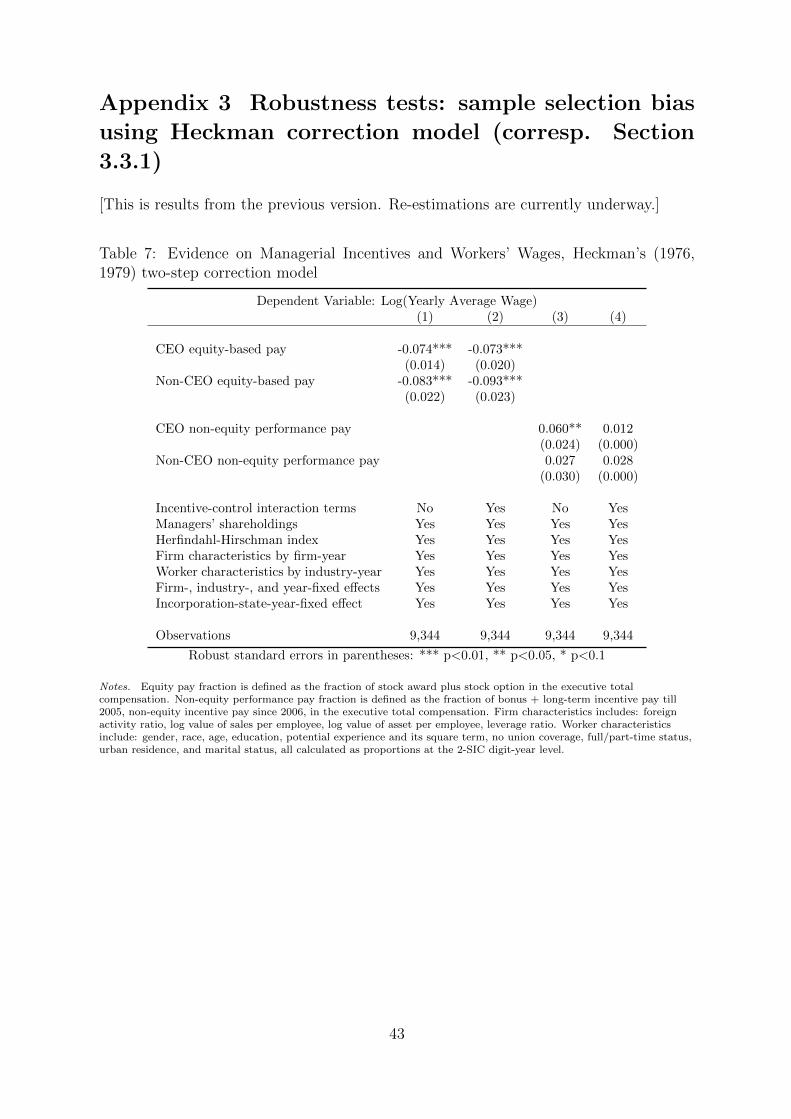
Appendix 3 Robustness tests: sample selection bias

using Heckman correction model (corresp. Section

3.3.1)

[This is results from the previous version. Re-estimations are currently underway.]

Table 7: Evidence on Managerial Incentives and Workers’ Wages, Heckman’s (1976,1979) two-step correction model

Dependent Variable: Log(Yearly Average Wage)(1) (2) (3) (4)

CEO equity-based pay -0.074*** -0.073***(0.014) (0.020)

Non-CEO equity-based pay -0.083*** -0.093***(0.022) (0.023)

CEO non-equity performance pay 0.060** 0.012(0.024) (0.000)

Non-CEO non-equity performance pay 0.027 0.028(0.030) (0.000)

Incentive-control interaction terms No Yes No YesManagers’ shareholdings Yes Yes Yes YesHerfindahl-Hirschman index Yes Yes Yes YesFirm characteristics by firm-year Yes Yes Yes YesWorker characteristics by industry-year Yes Yes Yes YesFirm-, industry-, and year-fixed effects Yes Yes Yes YesIncorporation-state-year-fixed effect Yes Yes Yes Yes

Observations 9,344 9,344 9,344 9,344

Robust standard errors in parentheses: *** p<0.01, ** p<0.05, * p<0.1

Notes. Equity pay fraction is defined as the fraction of stock award plus stock option in the executive totalcompensation. Non-equity performance pay fraction is defined as the fraction of bonus + long-term incentive pay till2005, non-equity incentive pay since 2006, in the executive total compensation. Firm characteristics includes: foreignactivity ratio, log value of sales per employee, log value of asset per employee, leverage ratio. Worker characteristicsinclude: gender, race, age, education, potential experience and its square term, no union coverage, full/part-time status,urban residence, and marital status, all calculated as proportions at the 2-SIC digit-year level.

43

Appendix 4 Robustness Tests: non-finance vs. fi-

nance; industry-year-fixed effects; managerial share-

holding (corresp. Section 3.3.2)

Table 8: Robustness Tests: Non-financial and financial sectors, industry-Year-Fixedeffects, CEO shareholding. Firm-level sample (corresp. Section 3.3.2)

Dependent Variable: Log(Yearly Wage)Non-finance Finance Industry-year Shareholding

(1) (2) (3) (4) (5) (6) (7) (8)

CEO equity-based pay fraction -0.053** -0.063 -0.057** -0.059***(0.022) (0.045) (0.023) (0.022)

CEO equity-based pay/salary ratio -0.004*** -0.001 -0.002 -0.002(0.001) (0.002) (0.002) (0.001)

CEO shareholding fraction -0.127 -0.085(0.177) (0.174)

Managers’ characteristics Yes Yes Yes Yes Yes Yes Yes YesFirm characteristics by firm-year Yes Yes Yes Yes Yes Yes Yes YesIndustry-year-fixed effects No No No No Yes Yes No NoWorker characteristics byindustry-year

Yes Yes Yes Yes No No Yes Yes

HHI by industry-year Yes Yes Yes Yes No No Yes YesFirm-, industry-, state-, and year-fixed effects

Yes Yes Yes Yes Yes Yes Yes Yes

Incorp-state-year-fixed effect Yes Yes Yes Yes Yes Yes Yes Yes

R-squared 0.402 0.404 0.372 0.369 0.473 0.472 0.307 0.305Observations 3,109 3,109 2,470 2,470 5,579 5,579 5,579 5,579Number of firms 368 368 286 286 651 651 651 651

Robust standard errors in parentheses: *** p<0.01, ** p<0.05, * p<0.1

Notes. Equity based pay fraction is defined as the fraction of stock award and stock option in the executive totalcompensation. Equity/salary ratio is defined as the value of stock award plus stock option divided by the value of salary.Manager characteristics include: gender, total amount of current compensations (salary + bonus), CEO-chair duality,externally-hired CEO, non-CEO’s gender. Firm characteristics includes: foreign activity dummy, sales per employee,total assets, leverage ratio, capital expenditure divided by total assets, and firm’s age. Worker characteristics include:gender, race, age, education, experience, union coverage, full/part-time status, urban residence, and marital status, allcalculated as proportions at the 2-SIC digit-year level. Robust standard errors are adjusted for clustering at the firmlevel.

44

Appendix 5 Robustness tests using the individual-

level sample: sample selection bias and composition

changes by offshoring (corresp. Section 3.3.3)

Data and Variables

Table 8 summarizes the distributions of workers, firms and executives across major sec-

tors in the individual-level sample, and Table 9 shows summary statistics of all variables.

Since we calculated the executive-, firm-, and industry-level variables at the 2-digit SIC

level, the discrepancies between the sectoral distributions of workers and firm/executive

do not affect matching and measurements. My sample contains 54 industries by 2-digit

SIC.

Table 9: Distributions of workers, firms and executives across major industries (%), theindividual-level sample

Sector (1-digit SIC, division) Workers Firms Executives

Mining and Construction 3.62 3.77 2.69Manufacturing 1: Food, Textile, Chemicals, etc. 8.86 13.16 15.04Manufacturing 2: Rubber, Machinery, Electronics, etc. 12.09 23.37 18.09Transportation, Communications, Electric, etc. 10.8 12.3 21.19Wholesale Trade & Retail Trade 25.35 13.57 8.51Finance, Insurance, and Real Estate 9.65 12.24 25.91Services 1: Hotel, Personal Business, Motion Picture, etc. 8.52 15.34 5.07Services 2: Health, Legal, Education, Social, etc. 21.12 5.89 3.51

In the analyses using the individual-level sample, the dependent variable is the

log(hourly wage), where the hourly wage includes annual wage and salary income28

plus employer’s contribution for health insurance, and divided by total working hours

and deflated by CPI to 2010 dollar values. It is therefore a measurement of a worker’s

total pay, keeping in line with the wage measure in the firm-level sample. (Table 5 col-

umn (3) and (4) show that the estimation results are similar when excluding employer’s

contribution for health insurance from the measurement of the dependent variable.)

Equity Fraction, Equity Ratio, and other manager and firm characteristics are defined

in the same ways as in the firm-level sample, but calculated at the industry-year level.

We first calculate them for each firm-year, and then take the weighted averages of each

at the 2-digit SIC level for each industry-year. We use the share of each firm in the

28 The data of extremely high incomes in CPS are subjected to topcoding procedures and thereforebias downward for confidentiality reason. To deal with the problem, we multiply top-coded incomes inthe period 1992-1995 by 1.75, following the method of Philippon & Reshef (2012).

45

total employees in each industry-year as the weight of each firm and each executive. So

the basic unit of my explanatory variables are a ratio in an industry-year. Individual

workers are then matched with the executive and firm variables by industry-year.

As in the previous firm-level analyses, we also include industry-, year-, and state-

year-fixed effects, and a Herfindahl-Hirschman index (HHI) based on the Compustat

dataset. Additionally, we control for occupation-fixed effects which is not feasible with

the firm-level sample.

46

Tab

le10

:V

aria

ble

sD

efin

itio

ns

an

dS

um

mary

Sta

tist

ics:

Ind

ivid

ual-

Lev

elA

naly

ses

Var

iab

leD

efin

itio

nM

ean

S.D

.M

inM

ax

Exec

uti

vean

dF

irm

Ch

arac

teri

stic

s,al

lfi

rst

calc

ula

ted

at

the

firm

-lev

el,

then

wei

ghte

dav

eraged

at

the

SIC

-yea

rle

vel.

(N=

1,1

27)

Hou

rly

wag

eA

nnu

alw

age

and

sala

ryin

com

esp

lus

emp

loye

r’s

contr

ibu

tion

toh

ealt

hin

sura

nce

(in

2010

doll

ar)

,d

ivid

edby

tota

lh

ou

rsw

ork

ed.

27.2

98

83.1

69

4.4

51

38,3

54

Log

(hou

rly

wag

e)H

ourl

yw

age

inlo

gari

thm

s.3.0

55

0.6

53

1.4

93

10.5

55

Man

age

r’s

com

pen

sati

on

stru

ctu

re,

byin

du

stry

-yea

rC

EO

equ

ity-b

ased

pay

frac

tion

Th

eC

EO

’seq

uit

y-b

ase

dp

ay(s

tock

award

s+

stock

op

tion

s)fr

ac-

tion

ofth

eto

tal

com

pen

sati

on

.0.4

42

0.1

24

0.0

75

0.7

49

CE

Ost

ock

awar

dfr

acti

onT

he

CE

O’s

stock

award

sfr

act

ion

of

the

tota

lco

mp

ensa

tion

.0.1

88

0.1

55

00.7

24

CE

Ost

ock

opti

onfr

acti

onT

he

CE

O’s

stock

op

tion

sfr

act

ion

of

the

tota

lco

mp

ensa

tion

.0.2

55

0.1

34

0.0

22

0.6

86

CE

Op

erfo

rman

cep

ayfr

acti

onC

EO

’sb

onu

s+

lon

g-t

erm

ince

nti

vep

ay+

equ

ity-b

ase

dp

ay,

till

2005

;C

EO

’sn

on

-equ

ity

ince

nti

ve

pay

+eq

uit

y-b

ase

dp

ay,

sin

ce20

06.

0.6

71

0.1

09

0.1

88

0.8

99

CE

On

on-e

qu

ity

per

form

ance

pay

frac

tion

Th

eC

EO

’sn

on-e

qu

ity

per

form

an

cep

ay(b

onu

s+

lon

g-t

erm

in-

centi

vep

ayti

ll2005,

non

-equ

ity

ince

nti

ve

pay

sin

ce2006)

fract

ion

ofth

eto

tal

com

pen

sati

on

.

0.2

26

0.0

89

0.0

13

0.4

72

CE

Oeq

uit

y-b

ased

pay

tosa

lary

rati

oT

he

CE

O’s

equ

ity-b

ase

dp

ay(s

tock

award

s+

stock

op

tion

s)d

i-vid

edby

sala

ry.

4.5

56

3.9

59

0.1

78

53.1

53

CE

Ost

ock

awar

dto

sala

ryra

tio

Th

eC

EO

’sst

ock

award

sd

ivid

edby

sala

ry.

1.8

99

2.3

74

0.0

00

51.9

17

CE

Ost

ock

opti

onto

sala

ryra

tio

Th

eC

EO

’sst

ock

op

tion

sd

ivid

edby

sala

ry.

2.5

99

3.1

36

0.0

74

42.8

33

CE

Op

erfo

rman

cep

ayto

sala

ryra

tio

CE

O’s

bon

us

+lo

ng-t

erm

ince

nti

vep

ay+

equ

ity-b

ase

dp

ay,

till

2005

;C

EO

’sn

on

-equ

ity

ince

nti

ve

pay

+eq

uit

y-b

ase

dp

ay,

sin

ce20

06.

Div

ided

by

sala

ry.

6.3

96

4.8

48

0.5

14

54.8

05

CE

On

on-e

qu

ity

per

form

ance

pay

tosa

lary

rati

oT

he

CE

O’s

non

-equ

ity

per

form

an

cep

ay(b

onu

s+

lon

g-t

erm

in-

centi

vep

ayti

ll2005,

non

-equ

ity

ince

nti

vep

aysi

nce

2006)

div

ided

by

sala

ry.

1.6

84

1.2

53

0.0

82

13.0

39

Non

-CE

Oeq

uit

y-b

ased

pay

frac

-ti

onF

irm

-ave

rage

dN

on

-CE

Oeq

uit

y-b

ase

dp

ayfr

act

ion

.0.3

57

0.1

09

0.0

00

0.6

66

Non

-CE

Ost

ock

awar

dfr

acti

onF

irm

-ave

rage

dN

on

-CE

Ost

ock

award

sfr

act

ion

.0.1

73

0.1

32

00.5

76

(con

tin

ued

)

47

(conti

nu

ed)

Var

iab

leD

efin

itio

nM

ean

S.D

.M

inM

ax

Non

-CE

Ost

ock

opti

onfr

acti

onF

irm

-ave

rage

dN

on

-CE

Ost

ock

op

tion

sfr

act

ion

.0.2

14

0.1

17

00.6

12

Non

-CE

Op

erfo

rman

cep

ayfr

ac-

tion

Fir

m-a

vera

ged

Non

-CE

Op

erfo

rman

cep

ayfr

act

ion

.0.5

86

0.1

05

00.9

09

Non

-CE

On

on-e

qu

ity

per

for-

man

cep

ayfr

acti

onT

he

Non

-CE

Oex

ecu

tive

s’n

on

-equ

ity

per

form

an

cep

ay(b

onu

s+

lon

g-te

rmin

centi

vep

ay)

fract

ion

of

the

tota

lco

mp

ensa

tion

.0.2

27

0.0

87

00.5

59

Man

age

r’s

chara

cter

isti

cs,

byin

du

stry

-yea

rC

EO

tota

lcu

rren

tco

mp

ensa

tion

CE

O’s

sala

ryp

lus

bonu

s.2,0

54.8

54

1,7

04.0

88

261.9

11

26,1

07.4

80

CE

O-c

hai

rd

ual

ity

1if

the

CE

Ois

als

oth

eb

oard

chair

,an

d0

oth

erw

ise.

0.6

23

0.2

35

01

exte

rnal

CE

O1

ifb

ecom

esC

EO

wit

hin

3ye

ars

of

join

ing

the

firm

,an

d0

oth

er-

wis

e.0.1

53

0.1

61

01

CE

Osh

areh

old

ing

Th

eC

EO

ssh

areh

old

ing

fract

ion

of

the

firm

’sto

tal

share

s.0.0

18

0.0

25

00.2

29

CE

Ore

lati

ve

shar

ehol

din

g1

ifth

eC

EO

own

sm

ore

share

sth

an

all

5%

inst

itu

tion

al

blo

ck-

hol

der

sto

geth

er,

an

d0

oth

erw

ise.

0.1

42

0.2

46

01

fem

ale

CE

O1

ifth

eC

EO

’sgen

der

isfe

male

,an

d0

oth

erw

ise.

0.0

20.0

63

01

Non

-CE

Osh

areh

old

ing

Fir

m-a

vera

ged

Non

-CE

Os

share

hold

ings

fract

ion

.0.0

03

0.0

06

00.1

27

Non

-CE

Ore

lati

ve

shar

ehol

din

g1

ifth

en

on-C

EO

manager

sow

ns

more

share

sth

an

all

5%

inst

i-tu

tion

alb

lock

hold

ers

toget

her

,an

d0

oth

erw

ise.

0.1

17

0.2

16

01

fem

ale

Non

-CE

O1

ifth

eN

on-C

EO

exec

uti

ve’s

gen

der

isfe

male

,an

d0

oth

erw

ise.

0.0

64

0.0

59

00.3

47

Fir

man

din

du

stry

chara

cter

isti

cs,

byin

du

stry

-yea

rL

og(s

ale

per

emp

loye

e)T

he

valu

eof

tota

lsa

led

ivid

edby

the

nu

mb

erof

emp

loye

es(i

nm

illi

ond

olla

r).

Inlo

gari

thm

s.5.4

32

0.7

48

2.5

64

8.3

78

Log

(ass

etp

erem

plo

yee)

Th

eva

lue

ofto

tal

ass

etdiv

ided

by

the

nu

mb

erof

emp

loye

es(i

nm

illi

ond

olla

r).

Inlo

gari

thm

s.5.5

02

1.1

43

1.6

20

8.7

96

Lev

erag

eT

otal

lon

g-te

rmdeb

tsan

dd

ebts

incu

rren

tli

ab

ilit

ies,

div

ided

by

tota

las

sets

.0.2

92

0.1

15

0.0

49

0.7

83

For

eign

Act

ivit

y1

ifth

efi

rmre

ceiv

esany

fore

ign

inco

mes

or

pay

sfo

reig

nta

xes

,0

oth

erw

ise.

0.6

72

0.2

83

0.0

00

1.0

00

(con

tin

ued

)

48

(conti

nu

ed)

Var

iab

leD

efin

itio

nM

ean

S.D

.M

inM

ax

Cap

ital

Exp

end

itu

res

Th

efu

nd

su

sed

for

ad

dit

ion

sto

pro

per

ty,

pla

nt,

an

deq

uip

men

t,ex

clu

din

gam

ounts

ari

sin

gfr

om

acq

uis

itio

ns.

InM

illi

on

sof

dol-

lars

.

1,1

65.9

89

2,0

86.8

48

8.7

14

20,5

26.2

36

Ret

urn

onas

set

Th

efi

rm’s

earn

ings

bef

ore

inte

rest

an

dta

xes

div

ided

by

the

valu

eof

tota

las

set.

0.0

93

0.0

43

-0.3

27

0.2

92

HH

IT

he

Her

fin

dah

l-H

irsc

hm

an

index

at

the

2-d

igit

SIC

-yea

rle

vel,

bas

edon

Com

pu

stat

data

set.

1,0

66.7

40

668.5

41

76.8

34

3,0

61.6

51

Ind

ivid

ual

Ch

ara

cter

isti

cs(N

=564,2

03)

Age

39.4

89

12.6

26

15

90

Fem

ale

1if

the

wor

ker’

sgen

der

isfe

male

,0

oth

erw

ise

0.4

79

0.5

01

Yea

rsof

Ed

uca

tion

No

sch

ool

:1;

1st

-4th

gra

de:

4;

5th

-8th

gra

de:

8;

9th

gra

de:

9;

10th

grad

e:10

;11th

gra

de:

11;12th

gra

de,

no

dip

lom

a:

11.5

;h

igh

sch

ool

grad

uat

e:12;

som

eco

lleg

e,n

od

egre

e:13;

ass

oci

ate

deg

ree:

14;

bac

hel

or’s

deg

ree:

16;

mast

er’s

deg

ree:

18;

pro

fess

ion

ald

egre

e:19

;d

oct

orat

ed

egre

e:23.

13.6

94

2.5

85

123

Exp

erie

nce

Pot

enti

alw

orkin

gex

per

ien

ceye

ars

,ca

lcu

late

dasmin{age−edu−

6;age−

18}

and

no

less

than

0.

19.6

06

12.5

38

072

Exp

erie

nce

2E

xp

erie

nce

squ

are

d541.6

18

574.1

20

5,1

84

Par

t-ti

me

Fu

ll/p

art-

tim

est

atu

s,1

ifth

ew

ork

eris

ap

art

-tim

ew

ork

er,

0ot

her

wis

e.0.1

54

0.3

61

01

Non

-wh

ite

race

1if

the

wor

ker

’sra

ceis

non

-wh

ite,

0oth

erw

ise.

0.1

95

0.3

96

01

No

un

ion

pro

por

tion

1if

no

un

ion

cove

rage,

0oth

erw

ise.

Th

isis

the

no

un

ion

cove

rage

rati

oca

lcu

late

dat

the

SIC

-yea

rle

vel.

0.7

99

0.1

17

0.1

29

1

Urb

anre

sid

ence

Aca

tego

rica

lva

riab

leco

ded

as:

0if

not

iden

tifi

able

;1

ifn

ot

inm

etro

area

;2

ifce

ntr

al

city

;3

ifou

tsid

ece

ntr

al

city

;4

ifce

ntr

al

city

stat

us

un

kn

own

.

04

Mar

ital

stat

us

Aca

tego

rica

lva

riab

leco

ded

as:

1if

marr

ied

,sp

ou

sep

rese

nt;

2if

mar

ried

,sp

ouse

ab

sent;

3if

sep

ara

ted

;4

ifd

ivorc

ed;

5if

wid

owed

;6

ifn

ever

mar

ried

/si

ngle

.

16

49

Model specification

We fit a series of cross-section regressions in the worker-firm-executive matched sample

as follows:

log(wijst) = α + βXjt + γMjt + δIjt + φVist + µFijst + εijst, (21)

where w is the hourly total wage, so log(wijst) is the log wage of individual i in industry

j in state s at time t. Xjt denotes CEO compensation structure measures of includ-

ing equity-based pay, stocks and options, performance pay, non-equity performance pay.

Mjt includes other manager characteristics and three variables of managerial control-

ling power. Ijt includes firm characteristics, and Vist includes workers’ characteristics

including occupation. Fjst are industry-, year- and state-year-fixed effects, and HHI

by industry and Emp-HHI by state. The robust standard errors are clustered at the

industry level. The estimations of β is of particular interest in the following analyses.

50

Table 11: Effects of Equity-Based Pay on Wages, Individual-Level Sample

Dependent Variable: Log(Hourly Wage)with health contrib. without health contrib.

(1) (2) (3) (4)

CEO equity fraction by industry-year -0.037*** -0.037***(0.011) (0.01)

CEO equity ratio by industry-year -0.000391** -0.000403**(0.000169) (0.000179 )

Manager characteristics by industry-year Yes Yes Yes YesHHI by industry-year Yes Yes Yes YesFirm characteristics by industry-year Yes Yes Yes YesWorker characteristics Yes Yes Yes YesOccupation-, industry- and year-fixed effects Yes Yes Yes YesState-year-fixed effect Yes Yes Yes Yes

Observations 564,203 564,203 564,203 564,203R-squared 0.51 0.51 0.502 0.502

Clustered-robust standard errors in parentheses: *** p<0.01, ** p<0.05, * p<0.1

Notes. Column (1) and (2): worker’s wage with employers’ contribution for health insurance. Column(3) and (4): worker’s wage without employers’ contribution for health insurance. Equity fraction isdefined as the fraction of stock award and stock option in the executive total compensation. Equityratio is defined as stock awards plus stock options divided by salary. Manager characteristics include:gender, total amount of current compensations (salary + bonus), CEO-chair duality, CEO’s relativeshareholdings against all other 5% institutional blockholders, externally-hired CEO, non-CEO’sgender, non-CEO’s relative shareholdings against all other 5% institutional blockholders. Firmcharacteristics includes: foreign activity dummy, log value of sales per employee, log value of asset peremployee, leverage ratio, numbers of employees, capital expenditure, return on asset, which are allcalculated at the 2-SIC digit industry-year level. Worker characteristics include: gender, race, age,education, potential experience and its square term, union coverage, full/part-time status, urbanresidence, and marital status. Robust standard errors are adjusted for clustering at the industry level.

51

Table 12: Effects of Four Compensation Components on Wages, Individual-Level Sample

Dependent Variable: Log(Hourly Wage)

(1) (2) (3) (4) (5) (6) (7) (8)

CEO stock award fraction -0.047**(0.018)

CEO stock option fraction -0.019*(0.01)

CEO performance pay -0.028**fraction (0.012)CEO non-equity perf. pay 0.03*fraction (0.018)

CEO stocks award ratio -0.000892***(0.000322)

CEO stock options ratio -0.000241(0.000159)

CEO performance pay -0.000368**ratio (0.000165)CEO non-equity perf. pay 0.000378Ratio (0.00152)

Manager characteristics byindustry-year

Yes Yes Yes Yes Yes Yes Yes Yes

HHI by industry-year Yes Yes Yes Yes Yes Yes Yes YesFirm characteristics byindustry-year

Yes Yes Yes Yes Yes Yes Yes Yes

Worker characteristics Yes Yes Yes Yes Yes Yes Yes YesOccupation-, industry- andyear-fixed effects

Yes Yes Yes Yes Yes Yes Yes Yes

State-year-fixed effect Yes Yes Yes Yes Yes Yes Yes Yes

Observations 564,203 564,203 564,203 564,203 564,203 564,203 564,203 564,203R-squared 0.51 0.51 0.51 0.51 0.51 0.51 0.51 0.51

Robust standard errors in parentheses: *** p<0.01, ** p<0.05, * p<0.1

Notes. Performance pay fraction is defined as the fraction of bonus + long-term incentive pay + equity-based pay, till2005; CEO’s non-equity incentive pay + equity-based pay, since 2006, in the executive total compensation. Stock awardand stock option fractions are defined as the value of stock award and stock option divided by the value of the executivetotal compensation. Stock award/salary ratio and stock option/salary ratio are defined as the value of stock award andstock option divided by the value of salary. Non-equity performance pay fraction is defined as the fraction of bonus +long-term incentive pay till 2005, non-equity incentive pay since 2006, in the executive total compensation. Managercharacteristics include: gender, total amount of current compensations (salary + bonus), CEO-chair duality, CEO’srelative shareholdings against all other 5% institutional blockholders, externally-hired CEO, and CEO’s non-equityperformance pay ratio, non-CEO’s gender, non-CEO’s relative shareholdings against all other 5% institutionalblockholders. Manager characteristics include: gender, total amount of current compensations (salary + bonus),CEO-chair duality, CEO’s relative shareholdings against all other 5% institutional blockholders, externally-hired CEO,non-CEO’s gender, non-CEO’s relative shareholdings against all other 5% institutional blockholders. Firmcharacteristics includes: foreign activity dummy, log value of sales per employee, log value of asset per employee, leverageratio, numbers of employees, capital expenditure, return on asset, which are all calculated at the 2-SIC digitindustry-year level. Worker characteristics include: gender, race, age, education, potential experience and its squareterm, union coverage, full/part-time status, urban residence, and marital status. Robust standard errors are adjusted forclustering at the industry level.

52

Reference

Almeida, H., Fos, V., & Kronlund, M. (2016). The real effects of share repurchases. Journalof Financial Economics, 119(1): 168-185.

Andrews, I., Stock, J., & Sun, L. (2018). Weak instruments in iv regression: Theory andpractice. Working Paper, Harvard University.

Angrist, J. D., & Pischke, J. S. (2008). Mostly harmless econometrics: An empiricist’s com-panion. Princeton university press.

Bakija, J., Cole, A., & Heim, B. T. (2012). Jobs and income growth of top earners and thecauses of changing income inequality: Evidence from US tax return data. Unpublishedmanuscript, Williams College.

Balsam, S., & Ryan, D. H. (2007). Limiting executive compensation: the case of CEOs hiredafter the imposition of 162(m). Journal of Accounting, Auditing & Finance, 22(4): 599-621.

Bebchuk, L., & Fried, J. (2006). Pay without performance. Cambridge, MA: Harvard Univer-sity Press.

Bell, Brian D. & John Van Reenen. (2013). Extreme Wage Inequality: Pay at the Very Top.American Economic Review, 103(3): 153-57.

Benabou, R., & Tirole, J. (2016). Bonus culture: Competitive pay, screening, and multitasking.Journal of Political Economy, 124(2), 305-370.

Bertrand, M., & Mullainathan, S. (1999). Is there discretion in wage setting? A test usingtakeover legislation. The Rand Journal of Economics, 30(3): 535-554.

Bertrand, M., & Mullainathan, S. (2001). Are CEOs rewarded for luck? The ones withoutprincipals are. The Quarterly Journal of Economics, 116(3), 901-932.

Bertrand, M., & Mullainathan, S. (2003). Enjoying the quiet life? Corporate governance andmanagerial preferences. Journal of Political Economy, 111(5), 1043-1075.

Bolton, P., Mehran, H., & Shapiro, J. (2015). Executive compensation and risk taking. Reviewof Finance, 19(6): 2139-2181.

Burkhauser, R. V., Feng, S., Jenkins, S. P., & Larrimore, J. (2012). Recent trends in topincome shares in the United States: reconciling estimates from March CPS and IRS taxreturn data. Review of Economics and Statistics, 94(2): 371-388.

Chemmanur, T. J., Cheng, Y., & Zhang, T. (2013). Human capital, capital structure, andemployee pay: An empirical analysis. Journal of Financial Economics, 110(2), 478-502.

Chen, C. R., Steiner, T. L., & Whyte, A. M. (2006). Does stock option-based executivecompensation induce risk-taking? An analysis of the banking industry. Journal of Banking& Finance, 30(3): 915-945.

Coles, J. L., Daniel, N. D., & Naveen, L. (2006). Managerial incentives and risk-taking. Journalof financial Economics, 79(2), 431-468.

Cronqvist, H., Heyman, F., Nilsson, M., Svaleryd, H., & Vlachos, J. (2009). Do entrenchedmanagers pay their workers more?. Journal of Finance, 64(1), 309-339.

Croson, R., & Gneezy, U. (2009). Gender differences in preferences. Journal of Economicliterature, 47(2), 448-74.

Cunat, V., & Guadalupe, M. (2009). Globalization and the provision of incentives inside thefirm: The effect of foreign competition. Journal of Labor Economics, 27(2): 179-212.

Dial, J., & Murphy, K. J. (1995). Incentives, downsizing, and value creation at General Dy-namics. Journal of Financial Economics, 37(3), 261-314.

Edmans, A., Fang, V. W., & Lewellen, K. A. (2017a). Equity vesting and investment. TheReview of Financial Studies, 30(7), 2229-2271.

Edmans, A., Gabaix, X., Jenter, D. (2017b) Executive Compensation: A Survey of Theoryand Evidence. In: Handbook of the Economics of Corporate Governance, Chapter 9., pp.

53

383-539.Edmans, A., Gabaix, X., & Landier, A. (2008). A multiplicative model of optimal CEO

incentives in market equilibrium. The Review of Financial Studies, 22(12): 4881-4917.Faleye, O., Reis, E., & Venkateswaran, A. (2013). The determinants and effects of CEO-

employee pay ratios. Journal of Banking & Finance, 37(8), 3258-3272.Fernandes, A. P., Ferreira, P., & Winters, L. A. (2018). The Effect of Competition on Executive

Compensation and Incentives Evidence from a Quasi-natural Experiment. Journal ofHuman Resources, 53(3): 783-824.

Giroud, X., & Mueller, H. M. (2010). Does corporate governance matter in competitive indus-tries?. Journal of Financial Economics, 95(3), 312-331.

Giroud, X., & Mueller, H. M. (2011). Corporate governance, product market competition, andequity prices. The Journal of Finance, 66(2), 563-600.

Gutierrez, G., & Philippon, T. (2016). Investment-less Growth: An Empirical Investigation.National Bureau of Economic Research Working Paper, No. w22897.

Handwerker, E. W., & Mason, L. G. (2013). Linking firms with establishments in BLS micro-data. Monthly Lab. Rev., 136, 14.

Handwerker, E. W., & Mason, L. G. (2014) Assessing the Usefulness of Census Bureau Multi-Establishment Data to Facilitate Linking Firms with Establishments in BLS MicrodataOctober 2014. JSM 2014 - Government Statistics Section.

Hart, O. D. (1983). The market mechanism as an incentive scheme. The Bell Journal ofEconomics, 14(2): 366-382.

Heckman, J. J. (1976) The Common Structure of Statistical Models of Truncation, SampleSelection and Limited Dependent Variables and a Simple Estimator for Such Models.Annals of Economic Social Measurement, Vol.5, No.4, pp.475-492.

Heckman, J. J. (1979) Sample Selection Bias as a Specification Error, Econometrica, Vol.47,No.1, pp.153-161.

Helpman, E. (2011). Understanding global trade. Harvard University Press.Hermalin, B. E. (1992). The effects of competition on executive behavior. The RAND Journal

of Economics, 23(3): 350-365.Hopkins, M., & Lazonick, W. (2016). The Mismeasure of Mammon: Uses and Abuses of

Executive Pay Data. Institute for New Economic Thinking Working Paper Series, No.49.

Jensen, M. C., & Meckling, W. H. (1976). Theory of the firm: Managerial behavior, agencycosts and ownership structure. Journal of Financial Economics, 3(4), 305-360.

Jensen, M. C., & Murphy, K. J. (1990). Performance pay and top-management incentives.Journal of Political Economy, 98(2), 225-264.

Jung, J. (2015). Shareholder value and workforce downsizing, 1981-2006. Social Forces, 93(4),1335-1368.

Jung, J. (2016). Through the contested terrain: Implementation of downsizing announcementsby large US firms, 1984 to 2005. American Sociological Review, 81(2), 347-373.

Krueger, A. B., & Summers, L. H. (1988). Efficiency wages and the inter-industry wagestructure. Econometrica, 56(2): 259-293.

Lazonick, W. (2014). Profits without prosperity. Harvard Business Review, 92(9): 46-55.Leonardi, M. (2007). Firm heterogeneity in capitallabour ratios and wage inequality. The

Economic Journal, 117(518): 375-398.Lin, K. H., & Tomaskovic-Devey, D. (2013). Financialization and US income inequality,

19702008. American Journal of Sociology, 118(5): 1284-1329.Melitz, M. J., & Redding, S. J. (2014). Heterogeneous firms and trade. In Handbook of

international economics (Vol. 4, pp. 1-54). Elsevier.

54

Murphy, K. J. (2013). Executive Compensation: Where We Are, and How We Got There.Handbook of the Economics of Finance, 2: 211-356.

Ordover, J. A., & Shapiro, C. (1984). Advances in supervision technology and economic welfare:a general equilibrium analysis. Journal of Public Economics, 25(3), 371-389.

Pagano, M., & Volpin, P. F. (2005). Managers, workers, and corporate control. The Journalof Finance, 60(2), 841-868.

Pathan, S. (2009). Strong boards, CEO power and bank risk-taking. Journal of Banking &Finance, 33(7): 1340-1350.

Perry, T., & Zenner, M. (2001). Pay for performance? Government regulation and the structureof compensation contracts. Journal of Financial Economics, 62(3): 453-488.

Philippon, T., & Reshef, A. (2012). Wages and human capital in the US finance industry:1909-2006. The Quarterly Journal of Economics, 127(4): 1551-1609.

Piketty, T., & E. Saez. (2003) Income Inequality in the United States, 19131998. QuarterlyJournal of Economics, 118(1), 2003: 139.

Raith, M. (2003). Competition, risk, and managerial incentives. American Economic Review,93(4): 1425-1436.

Rose, N. L., & Wolfram, C. (2002). Regulating executive pay: Using the tax code to influencechief executive officer compensation. Journal of Labor Economics, 20(S2), S138-S175.

Scharfstein, D. (1988). Product-market competition and managerial slack. The RAND Journalof Economics, 19(1): 147-155.

Schmidt, K. M. (1997). Managerial incentives and product market competition. The Reviewof Economic Studies, 64(2): 191-213.

Scopp, T. S. (2003). The relationship between the 1990 census and census 2000 industry andoccupation classification systems. Technical Paper, No. 65. Washington, DC: US CensusBureau.

Shin, T. (2014). Explaining pay disparities between top executives and nonexecutive employees:A relative bargaining power approach. Social Forces, 92(4), 1339-1372.

Shleifer, Andrei, & Lawrence Summers. (1988). Breach of Trust in Hostile Takeovers. InCorporate Takeovers: Causes and Consequences., edited by Alan J. Auerbach, pp. 33-56.Chicago: University of Chicago Press.

Shleifer, A., & Vishny, R. W. (1997). A survey of corporate governance. The Journal ofFinance, 52(2): 737-783.

Skott, P., & Guy, F. (2007). A model of power-biased technological change. Economics Letters,95(1), 124-131.

Skott, P., & Guy, F. (2013).Power, luck and ideology in a model of executive pay. Work-ing Paper (No. 2013-01). Abbreviated version published in Review of Radical PoliticalEconomics, 2013, 45(3), pp. 323-332.

Stock, J. H., & Watson, M. W. (2003). Introduction to Econometrics. Boston: Addison Wesley.Tirole, J. (1986). Hierarchies and bureaucracies: On the role of collusion in organizations.

Journal of Law, Economics, & Organization, 2(2), 181-214.Webber, D. (2018). The Rise of the Working-Class Shareholder: Labors Last Best Weapon.

Harvard University Press.

55