do parents selectively time birth relative to ramadan...
TRANSCRIPT

Do Parents Selectively Time Birth Relative to
Ramadan? Impact of Maternal Fasting on Height:
Evidence from Matlab, Bangladesh
Md. Nazmul Ahsan ∗
University of Southern California
February 28, 2014
PRELIMINARY AND INCOMPLETE.PLEASE DO NOT CITE
Abstract
When evaluating in utero nutrition shock, many studies assumeparents do not selectively time birth relative to that event of shock.Fasting during Ramadan is one of the nutrition shocks. Using MHSS1996 data we show that Muslim mothers who received free contracep-tives timed the birth of their children relative to Ramadan. We alsoevaluate the consequence of allowing selection. When we do not con-trol for selection, we find maternal fasting has adverse effect on height.However, when selection is controlled we do not find any statisticallysignificant effect on height.
1 Introduction
There is a growing literature based on “Fetal Origin Hypothesis”(Barker1990) which links adverse environment and the inadequate nutrition in uteroto later life health outcomes. Numerous evidences from these studies shownine months in utero is very critical for individual health (Almond and Cur-rie 2011). Adverse condition in utero can have both short term effect suchas effect on birth weight and long term effects such as effect on cognition,
∗I am indebted to John Strauss and Anant Nyshadham for their continuous guid-ance and advice on this paper. Suggestions from Ummul Hasanath Ruthbah,MohammadHashem Pesaran, Fei Wang and discussions with Rakesh Banerjee, Riddhi Bhowmick wereessential to this research. All remaining errors are my own. Any comments are welcome.Email :[email protected]
1

obesity, cardiovascular disease, diabetes (Almond and Muzumder 2011, Al-mond and Currie 2011, Ewjik 2011). The early studies, however, did nottake into account the endogenous exposure to adverse environmental andnutritional condition (Almond and Currie 2011). As a result they couldnot address potential confounders appropriately. To establish causal linkbetween in utero nutrition shock and health outcomes researchers studiednutrition and health shocks in utero exogenous to mothers(Currie 2009).Some of the studies are based on severe historic events such as famine andspread of infectious disease and recent few studies are based on regular occur-ring event such as Ramadan (Almond 2006; Chen and Zhou 2007; Almondand Muzumder 2011; Ewjik 2011 and Majid 2012). The results from thesestudies conform with the hypothesis that adverse nutritional environmentin utero has serious consequences on child health.
However, these studies are not free from limitations. One importantmethodological limitation is that they are based on the assumption thatparents don’t selectively time birth relative to those shocks. Thomas(2009)suggests that it is a strong identifying assumption and may not hold. Usingdata on famine in Bangladesh and Influenza Pandemic in USA, he finds thatparents who gave birth relative to these events were systematically differentfrom those who didn’t. This raises a serious concern as we do not knowwhether the results are driven entirely by selection or shocks in utero.It isvery important to examine the results to discern between selection effect andnutritional shock effects . This has important policy implications. Imaginewe find that one particular in utero nutrition shock affects health outcomesnegatively controlling for selective timing of birth. Then we have to formpolicies to address this issue. We know from the literature that nutritionshock in utero has persistent effect throughout an individual’s life. This willcreate an inequality at birth which can not be reversed. Therefore, we haveto take measures to save pregnant mother from such nutritional shock. Onother hand, imagine we don’t find any effect after taking care of selection.This would imply that the particular in utero nutrition shock under studyhas no effect on child health and we do not need to form any policies totackle this.
In this paper we study the impact of in utero nutrition shock due to ma-ternal fasting during Ramadan on child health accounting for selective tim-ing of birth using Matlab Health and Socioeconomic Survey(MHSS) 1996.The quasi-random placement of family planning program in Matlab allowsus to examine whether mothers selectively time birth relative to Ramadan.Empowered with this treatment, we instrument the time of birth relativeto Ramadan to study the impact of nutrition shock due to maternal fast-
2

ing during Ramadan on child height. Typically, the literature studies birthweight to measure the impact of nutrition shock in utero. Unfortunately,MHSS does not have any information of child birth weight. However, Currieand Vogl(2012) argues height can be a good proxy for birth weight. Medicalliterature also suggests that height reflects the combination of both genotypeand phenotype influences in utero (Martorell and Habicht 1986). Moreover,in economics literature height has been positively associated with wage andproductivity. (Strauss and Thomas 2008). There is huge policy value of thisstudy. Almond and Muzumder(2011) estimates roughly 1 billion of Muslimsalive today were in utero during the month of Ramadan.
Broadly, we present two main results. First, we find that Muslim moth-ers time birth relative to Ramadan. This result is consistent with variousrobustness checks. Secondly, we instrument time of birth relative to Ra-madan with the family planning program placement to get causal estimateof impact of maternal fasting on height. In contrast to earlier findings, wedon’t find any evidence adverse effect of maternal fasting on children heightcontrolling for selection.
This paper makes some key contributions in the literature. First, weshow parents selectively time birth relative to Ramadan using a rich dataset. In our knowledge this is the first paper that shows selective timing ofbirth relative to Ramadan. Secondly, we find that community level timevarying characteristics affect timing of birth.This suggests comparison ofSES of the parents of an affected child with the parents of a non-affectedchild may not be adequate to determine selection in birth timing. Thirdly,we show that providing free contraceptives may help Muslim mothers toavoid pregnancy overlapped with Ramadan. Past literature has evaluatedthe free contraceptive program in Matlab on fertility, health and educa-tion. This paper is the first to evaluate the family planning program in thecontext of Ramadan fasting. Fourth and most importantly, the paper at-tempts to study the impact of nutrition shock in utero on health outcomessystematically taking into account selective timing of birth.
The rest of the paper is organized as follows. In section 2 we briefly thediscuss existing literature on maternal fasting on different outcomes fromepidemiology and economics. In section 3 we discuss the background ofMatlab Family Planning and Child Health Program. In Section 4 we discussthe MHSS and compare it with other data sets used in the literature. Insection 5 the we discuss the empirical strategy to study selective timingof birth relative to Ramadan and also how it affects health outcomes. Insection 6 we provide the results and also discuss the contrast and similarityof these results with existing literature. In section 7 we make concluding
3

remarks.
2 Literature Review
The literature on maternal fasting on child health outcomes can be broadlydivided into two categories. One category is epidemiological literature andanother is economics literature. Almond and Muzumder(2011) presents anice summary of epidemiological literature in their paper. Several studiessuggest that fasting during pregnancy can lead to neurological impairments,higher blood pressure in later life (Hunter and Sadler 1987,Moore et al.1989, Sheehan et al. 1985, Gluckman and Hanson 2005).
Almond and Muzumder(2011) notes some limitations of epidemiologicalstudies. First of all, most of those studies are based on a small number ofobservations. Secondly, those studies compare the effect on fasters and non-fasters assuming that decision to fast is exogenous. Thirdly, those studiesdo not disentangle the fasting effect from the seasonality, as they are basedon Ramadan overlapping with only one season.
The application of Intent To Treat (ITT)analysis distinguishes the studyof Almond and Muzumder(2011) from the epidemiological studies on Ra-madan. They were also were first to study the impact of maternal fastingduring Ramadan on child outcomes in the economics literature. ITT anayl-sis alllows them to get rid of the compliance problem related to fasting.Under the assumption that parents do not selectively time birth relativeto Ramadan, it gives causal estimates of the impact of in utero nutritionshock. Moreover, unlike most epidemiological studies, the study of Almondand Muzumder(2011) was also based on a large number of cohorts.
Almond and Muzumder(2011) use data from Michigan, Iraq and Uganda.They study the impact of in utero nutrition shock on birth weight using datafrom Michingan and on various forms of disabilities using census data fromIraq and Uganda. They find children who were in utero during Ramadanhave lower birth weights and are more likely to be disabled. Following Al-mond and Muzumder(2011), Ewjik(2011) finds that maternal fasting duringRamadan may increase the chances of developing health problem such ascoronary heart disease and type 2 diabetes. Majid(2012) finds that maternalfasting during Ramadan leads to fewer hours worked and self-employmentin later life. Ewjik(2011) and Majid(2012) use Indonesia Family Life Sur-vey(IFLS) wave 3 and wave 4 respectively. Using English register data,Almond Muzumder and Ewjik(2012) finds that maternal fasting during Ra-madan leads to lower test scores.
4

One obvious limitation in those papers is that they assume parents don’tselectively time birth relative to Ramadan. Moreover,the above mentionedstudies have serious some limitations with data. In Michigan and Iraq data,Almond and Muzumder(2011) didn’t know the religion of the mother. Theyused Arab as proxy for Muslims in their Michigan data. The birth datafrom Uganda, Iraq and Indonesia were self-reported. This could be a seriousproblem as misreported birth dates will lead to wrong classification of birthrelative to Ramadan. In comparison to past data sets used, with MHSS wecan clearly identify the religion of the mother and get reliable birth data ina single data set for a sufficiently large of number of cohorts.
3 Matlab Family Planning and Child Health
Matlab is a thana(sub-district) in Chandpur District in Bangladesh. It islocated 55 kilometers of South-East of Dhaka. The Demographic Surveil-lance System(DSS) has been operating in Matlab thana since 1966. Initially132 villages were included in the system, and 101 villages were added in1968.All households in the DSS area are within the Monitoring system. Atypical village consists of several baris, or groups of houses around a centralcourtyard. In DSS area, the record of birth, death and migration(in and out)are collected from the start of the project. The enumeration of marital unionand dissolution began in 1975(Razzaque and Streatfiled). In October 1977the DSS area was contracted to 149 villages by excluding 84 villages. Thefamily planning and health project was launched in 70 villages(treatmentarea)and the remaining villages were comparison area. No report of usingrandomization mechanism has been found (Schultz 2009). The figure (1)1 inappendix also shows that the treatment area grouped into clusters.Schultz(2009) argues that the clustering of villages into treatment area retain thespillover effect. Table 3 in appendix presents 1974 census data which showsthat the treatment and the comparison area were very similar except forfew observable characteristics such as sources of drinking water, number ofcows and age of both household head and spouses of household head. In ourestimation strategy we will control household and biological sibling fixedeffects to account for the household and mother level fixed unobservables.
Barham(2012) also describes the other treatments added to the treat-ment areas which are documented in Bhatia et al.(1980), Phillips et al.(1984)and Koening et al.(1990). In October 1977, the family planning programbegan in treatment areas through the provision of modern contraception.
1Figure 1, table 2 and 3 are reproduced from Bahram (2012)
5

From June 1978, pregnant women received tetanus toxoid vaccination andalso pregnant women in their last trimester pregnancy received iron andfolic acid tablets. From March 1982, the children aged from 9 months to 59months in treatment area 1 received measles vaccine. This program was ex-panded to treatment area 2 on November 1985. From January 1986, DPT,polio and tuberculosis immunization were given to children under age 5.Later in 1986, Vitamin A supplementation for children under age 5 andnutritional rehabilitation for those who were nutritionally risky were addedto treatment areas. In appendix section, I reproduced the table 1 fromBarham(2012) which gives a summary of the programs introduced in thetreatment areas and age cohorts the programs have affected.
4 Data
This paper uses Matlab Household and Socioeconomic Survey 1996 whichwas funded by National Institure of Aging and was collaborative effort ofRAND, the Harvard School of Public Health, the University of Pennsylva-nia and the University of Colorado at Boulder . The primary sample wasdrawn from a probability sample of 2,883 baris from 7,440 baris in the DSS1994 sample frame. baris usually consists of cluster of households in closephysical proximity. In all baris, interviews were completed in 2,781 baris outof 2883 eligible baris. Within each bari, upto two households were randomlyselected. For each baris, one household was randomly chosen and designatedas primary household or Status = 1. If there are more than 2 households,the second household was randomly chosen and designated as Status = 2.Otherwise the second household was designated as Status = 2. Out of the2,781 baris, 94 baris were inappropriately interviewed and therefore disre-garded from analysis which leaves us with 2,687 baris. Out of these baris,656 are one household baris and rest of them have two or more households.Ideally, there should be 2,013 households but the survey team could findonly 1,677 households. The remaining Status = 2 households are purposivesample based on relationship to the first household. In this paper we limitour studies to only Status = 1 households or primary households.
In the survey mothers were asked about birth dates of each their chil-dren. Later the birth dates were matched with the DSS data sets for theirconsistency and accuracy. Although DSS started in 1966, during the datacollection process of MHSS the events(i.e. birth, marriage) which took placefrom 1974 were linked to computerized system of DSS. Therefore, we havereliable birth dates for 22 birth year cohorts from 1974 to 1995. All birth
6

dates before 1974 are self reported (Menken et al. 1999). There are also someother limitations with this data. We get the birth data from the pregnancyhistory of the women interviewed in the MHSS 1996. This is a limitationbecause we can know about births prior to 1996, only if the women living insampled household survived till 1996. Since the treatment area got maternalhealth care, one might argue that the women who survived in treatment areamay not have survived in absence of maternal health treatment.Ronsmanset al.(1997) finds that maternal mortality from all causes declined in bothtreatment and control area from 1976 to 1993 and the difference is no signif-icant between treatment and control areas. Moreover, if the survival of thewomen correlates with birth timing relative to Ramadan, this will create adownward bias. To illustrate, let’s suppose there are two types of womenhigh type and low type. High type avoids birth and low type doesn’t avoidbirth relative to Ramadan. The low type is also less likely to survive. Thematernal health aspect of the treatment would make it more likely that thelow type survives in the treatment area and therefore get included in thesample.Another limitation of the data is for some births only month and year ofbirth is known and the birth dates are replaced with zero. It also varies con-siderably between treatment area and control area. There are 2086 birthswhich had date zeros out of 8573 from 1974 to 1995. Out of the 2086 births,the treatment area had 856 births and control area had 1230 births. Onepossibility is that some of these births took place out of the treatment andcontrol area. Another possibility is these births have date zeros because ofbirth data collection method. We will do the analysis both including andexcluding these date zero births.
To study the impact on height we match the birth dates from the mother’spregnancy with the birth month and year of the individual surveyed in theMatlab. We later match anthropometric data for each individual. We limitour study to only single birth. There are few twin births in MHSS. We foundonly 28 twins in our data.
5 Ramadan Measures
The month of Ramadan is the 9th Month in the Islamic Calender Year.Islamic law does not require a pregnant woman to fast during pregnancy.However, evidence from different Muslim countries suggests that some Mus-lim mothers fast when they are pregnant(Almond and Muzumder 2011).
For a given year, we construct the dates Gregorian Calender which over-
7

laps with the Ramadan Month of Islamic Calender 2. From our birth datawe only know the date of birth but we don’t know the gestation time. Weobserve how many months after Ramadan the individual ‘i’ was born. Gen-erally, the gestation time for human is 266 days. For each date of birthwe create century day code(CDC) following Almond and Muzumder(2011).We will denote ramadan 0 if the individual ‘i’ was born during Ramadan,ramadan 1 if the individual ‘i’ was born within 30 days after Ramadan,ramadan 2 if the individual ‘i’ was born between 31 days and 60 days afterRamadan and so on. We also define dummy variable 1 if individuals wereborn between X and Y months after Ramadan asRamadanXtoY whereX <Y and 0 otherwise. For example, ramadan7to9 would mean anyone whoborn between 180 to 270 days after Ramadan. ramadan7to9 would mean theindividuals were most probably in the first trimesters when Ramadan over-lapped with pregnancy. Similarly, ramadan4to6 and ramadan1to3 wouldmean individuals were most probably in second trimester and third trimester.We prefer to use ramadan7to9 in stead of first trimester because we onlyknow the date of birth. At times birth takes place preterm and post-term.As a result, if we denote ramadan7to9 as first trimester, we would wronglyclassify first trimester overlapped with Ramadan.
For individuals whose date of birth is not known or date of birth isreplaced with zero, we match the month of Gregorian Calender year withRamadan Month and replace the month of Gregorian Calender year with 1 ifmore than 50 percent or more of Ramadan days overlap with the GregorianMonth.
6 Estimation Strategy
Empirical strategy is divided in two sections. In the first section we testwhether parents selectively time birth relative to Ramadan. In the secondsection we study the impact of maternal fasting of height. Most of theanalysis is based on cohorts born from 1974 to 1995 because Schultz(2009)and Schultz and Joshi(2007) find that the treatment and control area werebalanced in many dimensions. As a robustness check, analysis on birthcohorts born from 1963 to 1995 was also conducted.
2Following Almond and Muzumder(2011), we construct the Ramadan monthfrom Institute of Oriental Studies at University of Zurich using their websitehttp://www.oriold.uzh.ch/static/hegira.html
8

6.1 Selection on Timing of Birth
We run the following regression equation to test this assumption:
Rijhkmt = β0 + β1Post+ β2Treated+ β3Treatment+ β4Hindu
+ β5Post ∗Hindu+ β6Treated ∗Hindu+ β7Treatment ∗Hindu+ β8X
+ αj + νh + γm + δt + τk + εijhmt (1)
Equation (1) basically means whether individual i, born by mother j inmonth m and year t, was in utero during Ramadan or not. The post variabletakes value 1 if the individual was born in July in 1978. The Treated valueis 1 if the person living in a village which gets the treatment and 0 oth-erwise. Although the program started in October,1977. The variable posttakes value 1 from July 1978 and 0 otherwise. The reason is those who wereborn between October 1977 and July 1978 were conceived prior to programstarted. We can identify post even with year fixed effect because of the startof the program in middle of the year. The Treatment is the interaction be-tween Treated and Post. αj is the mother fixed effect, νh is household fixedeffect, γm is the month fixed effect, δt is the year fixed effect and τk is thevillage fixed effect. R represents several outcome variables. From our dis-cussion on measures of Ramadan, R represents various Ramadan measuresramadan 0 to ramadan 10 and ramadanXtoY for various values of X andY where X < Y .The Hindu dummy is 1 if the the mother is Hindu and 0otherwise. The interaction term of Hindu with Post, Treated and Treatmentallows us to check robustness of the avoidance behavior of Muslim mothersrelative to Ramadan. The variable X represents community variables andinteraction of the community level variables with post. The communitylevel variables are whether the village has large market, electricity, postoffice, primary school and satellite health clinic.
6.2 Impact on Health
We want to know how Ramadan affects on health taking care of selectivetiming of birth relative to Ramadan. Therefore we are interested in followingregression equation
YMiabjhkmt = µ0+µ1Post+µ2Treated+µ3R+µ4Sexc+αj+νh+γm+δt+τk+uiabjhkmt
(2)Where YM
iabjhkmt is the height in centimeters and of the Muslim individual‘i’,born by mother ‘j’ in month‘ m’ and year ‘t’ , who belongs to age groupa,household h and village k. Sexc is the sex of the children.
9

However, the various treatments added to the treatment area make ithard to disentangle the benefit on health between avoiding birth relativeto Ramadan and the treatments. In other words, we have to worry aboutthe exclusion restriction of the instrumental variable. We construct thevarious age groups to capture the different treatment effects on the age groupfollowing Barham(2012) The study on height is only limited to 22 birth yearcohorts. In this study age group 1 are the individuals who were born fromJanuary 1974 to September 1977, age group 2 are the individuals who wereborn in October 1977 to February 1982, age group 3 are the individuals whowere born in March 1982 to December 1988 and the remaining individualsfall in age group 4. The treatment area is interacted with the age groups tocapture age specific treatment effects. Following Barham(2012) we regressfollowing regression equation:
Yiabjhkmt = ρ0+ρ1Ti+ρ3sexci+
4∑s=2
πsdis+
4∑s=2
φsdis∗Ti+αj+νh+γm+δt+τk+εiabjhkmt
(3)The omitted category is the age group 1. The dis is dummy for age
group 2 to 4. The dummy variable takes value 1 if individual i belongs toage group s and 0 otherwise. The variable Ti takes value 1 if individual i isfrom treated area and 0 otherwise. We will run the regression equation onHindu population in our sample to get the treatment effects of the additionaltreatments in the treatment area. We will subtract the treatment effects onthe specific age groups from the height of Muslim population to calculatethe magnitude of impact of fasting on height.
We also estimate the impact of first, second and third trimester overlap-ping with Ramadan on height with following regression equation:
Yijhkmt = Γ0 + Γ1ramadan1to3 + Γ2ramadan4to6 + Γ3ramadan7to9
+ Γ4Hindu+ Γ5Sexc+ Γ6Hindu ∗ Sexc+ Γ7ramadan1to3 ∗Hindu+Γ8ramadan4to6∗Hindu+Γ9ramadan7to9∗Hindu+αj+νh+γm+δt+τk+ξiabjhkmt
(4)
7 Results
7.1 Selective Timing of Birth
To study selective timing of birth we regress ramadan0 to ramadan10 onpost, treated and treatment for Muslims controlling for birth month and year
10

fixed effects. The cohorts under study were born from year 1974 to 1995.The results are presented in table 1. We find that treatment has statisticallysignificant positive effect on individuals being born in ramadan 5 and nega-tive effect on ramadan 9. This leads us to construct variables ramadan5to6,ramadan5to7 and ramadan8to9 where for example ramadan8to9 takes value1 if individual i is born either during ramadan8 or ramadan9 and 0 other-wise and regress these variables with the same independent variables. Thebirth pattern of Hindus relative to Ramadan works as a robustness check. We should expect the variables Hindu and post, treated and treatmentinteracted with Hindu should not be statically significant from zero. Wealso would like to check the robustness of our results with regression spec-ifications with household fixed effects and biological mother fixed effects.The results are presented in table 2. The dependent variables from column1 to 3, from 4 to 6 and from 7 to 9 are ramadan5to6, ramadan5to7 andramadan8to9 respectively. All regression specifications include birth monthand year fixed effects. In column 1 we find the coefficient of the treatmentvariable is positive and statistically significant from zero. On the other hand,in column 2 and 3 when household fixed effects and biological mother fixedeffects are applied, it is positive but not statistically significant. In column4 to 6, we find that the treatment coefficient is positive and statisticallysignificant when regression specifications include birth month and year fixedfixed effects as well as household fixed effects. However, it is not statisti-cally significant when biological fixed effects are applied. In column 7 to 9,the treatment coefficient is negative and statistically significant in all fixedeffect regression specifications. As we would expect the variable Hindu andinteraction terms with Hindu are not significantly different from zero in allcolumns and all regression specifications. Since ramadan5to7 incorporatesramadan5o6, we omit the analysis on ramadan5o6 in the following results.
In MHSS data we find that more births take place on date 1 than anyother dates. Moreover, data shows unusually high amount of birth birthtakes place on January 1st than any other day of the year. We try to checkthe further robustness of our results in table 2 by dropping these dates. Intable 3 we replicate our exercise by dropping date 1. We find the the resultsare robust to dropping these dates. In table 4 we drop the births takenplace on January 1st and we find that the treatment coefficient is staticallysignificant for all regression specifications. The results in table 4 is evenmore robust than the results in table 2. This suggest there might be somemisreporting of birth dates in Matlab data. We don’t know which birth tookplace in Matlab and which didn’t. It is quite possible some of these birthsactually took place out of surveillance area and were not registered in DSS.
11

Recall that we can identify the variable post in our regression equationeven though we have year fixed effects because of the timing of the program.To check whether this does not corrupt our estimates we redefine post wherepost takes value 1 for 1979 and onward and 0 otherwise. This does not allowus to identify post as the variable post is absorbed by year fixed effects. Wedo same exercise of table 2 with redefined post variable. The results arepresented in table 5. We find that results are consistent with our results intable 2.
So far we have limited our analysis to birth dates known in MHSS. InMHSS data there are some births which have dates recorded zero. Theresults are presented in table 6. We find that the treatment coefficient isnegative for ramadan8to9 and positive for ramadan5to7 as in table 2. Fordependent variable ramadan5to7 the treatment coefficient is positive andstatistically significant when household fixed effects are included. However,it is not statistically significant in a regression specification with biologicalmother fixed effects. For variable ramadan8to9 the treatment coefficient isnegative and significant in regression specification with month and year fixedeffects. However, it is not statistically significant when household fixed ef-fects and biological fixed effects are included in the regression specifications.
We again limit our analysis to population whose birth dates are knownand further check the robustness by studying the birth cohorts born from1963 to 1995. This gives us 33 birth year cohorts. Recall that it takesRamadan around 32 to 33 years to complete a full circuit of western calender.The results are presented in table 7. The results conforms with the findingsin table 2.
In table 8 we control for village level characteristics and do the sameanalysis in table 2 for cohorts born from 1974 to 1995. We find that evenincluding village level characteristics and interacting them with post do notalter our findings.
In table 9 we study the relationship between timing of birth relativeto Ramadan with mother education level. The primary takes value 1 ifmother education ranges between more than 0 to less than 6 and 0 otherwise.The secondary education takes value 1 if mother has more than 5 years ofeducation and 0 otherwise. The mother education variables are interactedwith post treated and treatment variable. What we find is the primaryeducated are less likely give birth during ramadan8to9. The are also morelikely to avoid birth using the contraceptive treatment.
In table 10 we study the avoidance behavior with mother education inyears. The mothereduy variable takes value the years of education com-pleted by mothers. We find that for variable ramadan8to9 the treatment
12

coefficient is negative and statistically significant. However, the interactionterms with mother education in years with post treated and treatment isnot statistically significant.
7.2 Discussion on Selective Timing of Birth
Based on the results from table 1 to 8 we can conclude that the Muslimmothers are selectively timing the birth of their children relative to Ra-madan. Our results show mothers in the treatment area are around 6 per-cent less likely to give birth 8 or 9 months after Ramadan and more likelyto give birth 5 to 7 months after Ramadan. The avoidance results are ro-bust to inclusion of biological mother fixed effects. Biological mother fixedeffects control mother level fixed unobservables that might affect the tim-ing of birth and also affect health outcomes of the children. Ewjik(2011)and following Ewjik(2011), Majid(2012) motivates to solve the problem ofselective timing of birth by controlling biological mother fixed effects. Ourresults suggest controlling biological mother time invariant unobservablesmay not be enough to take care of selection. We find that Muslims mothersare shifting the births few months ahead and avoiding conception just oneor two months before Ramadan. The question is why do we observe suchpattern? If the mothers worry that fasting during pregnancy could affectthe child health negatively, they would choose a time period where the preg-nancy doesn’t overlap with Ramadan. Perhaps they don’t do it because it isreally hard to time birth in that way. The gestation time for human is 266days and the Islamic Calender completes a year in 354 or 355 days. Thatleaves mothers 88 or 89 days to give birth to completely avoid Ramadan.Another possibility is that mothers are shifting the births ahead to avoidfasting during Ramadan. It could be possible that when child in utero is fouror five months older at the time of Ramadan, the family members, friendsand relatives are less likely to ask the mother to fast during Ramadan
In table 9 we study the association between mother education level withthe timing of birth relative to Ramadan. We find the mothers who hadsome education but less than equal to primary education are more likelyavoid conception 1 or 2 months before Ramadan than others. On otherhand the mothers who have more than primary education do not time birthrelative to Ramadan. This points out the avoidance behavior is not linearlyrelated to mother education or in other words more education of mothersdoesn’t mean that they are more likely to avoid birth relative to Ramadan.However, this shouldn’t mean that more educated mothers do not care abouttheir children. It could be possible that they are informed about Islamic
13

rules about fasting for pregnant mothers. According to Islamic law it isnot mandatory for Muslims mothers to fast during pregnancy. The motherswith more education are more likely to know about it than mothers withlow education. However, if the mothers are somewhat educated like primaryor below they might still suffer from the belief that they have to fast duringRamadan even if they are pregnant or they may belong to SES where thesocial pressure is high for fasting during Ramadan even with pregnancy. Themothers with primary and below education are more likely to avoid birthbecause they would have some idea about calender and time of Ramadanthan mothers with no education. Therefore, they are more likely to use thecontraceptive treatment to time birth relative to Ramadan .
7.3 Effect of Maternal Fasting on Height
In table 11 we study the impact of maternal fasting overlapped with firsttrimester second trimester and third trimester on children height for cohortborn from 1974 to 1995. As discussed above ramadan7to9 should be in-terpreted as first trimester, ramadan4to6 should be interpreted as secondtrimester and ramadan1to3 should be interpreted as third trimester. Wealso interact the Hindu with these variables to cancel out any seasonalityeffect. We find that the coefficient of ramadan7to9, ramadan4t06 and ra-madan1to3 all are negative. However, only ramadan7to9 and ramadan1to3are statistically significant when we control for month and year fixed effects.Only coefficient of ramadan7to9 is robust to inclusion of village level fixedeffects. These variables are not statistically significant when we control forhousehold fixed effect and biological mother fixed effects. As we would ex-pect, the variable Hindu and interaction hindu with Ramadan variables arealso not significant in any regression specification.
Next we study the impact on height if the children were born 8 or 9months after Ramadan or in other words we regress height on ramadan8to9on height and compare with children born in Hindu families during thesame time. The results are presented in table 12. We find the variableramadan8to9 is negative and statistically significant and the result is robustto inclusion of village level fixed effects.
This demands us to examine the impact on height taking care of theselective timing of birth. The problem is that the exclusion restriction re-quirement of the instrument may not hold. We replicate the exercise ofBarham(2012) to get the magnitude of the effect of these treatments onchildren height in centimeter for cohort born from 1974 to 1995. The resultsare shown in table 13. Column 1 and 2 show results on overall population,
14

column 3 and 4 show results on Muslim and column 5 and 6 show resultsonly for Hindu. In Column 1 and 2 we find that only age group 3 havebenefited from the later treatments in treatment area. This result matcheswith the findings of Barham(2012). We also find similar results for Hindupopulation. However, for Muslims only the column 3 and 4 show there is noeffect.
In table 14 we show our results on height after taking care of selection.In column 1 and 2 we present first stage and second stage results respec-tively. In column 1 and 2 we disregard any exclusion restriction problem.We therefore instrument ramadan8to9 with treatment controlling for vil-lage level fixed effects. In column (2) we find that instrumeted variable
ˆramadan8to9 is negative but not significantly different from zero. We con-struct a variable mheight to tackle the problem of exclusion restriction.Under the assumption the treatments added to treatment area had lineareffect on the height of the children, we can subtract the effect of those treat-ments from the height. Fortunately, the Hindus and Muslims in the areareceived the same treatment in the treatment area. So we can study theaverage treatment effect of those treatments on the Hindu population andsubtract it from height of the Muslims living in the treatment area. Themheight is created by subtracting the effect of those treatments on Hindusfrom height for age group 3. Then we regress mheight on ˆramadan8to9.The result is shown in column 3. We find that the coefficient is positivebut not significantly different from zero. We then again construct anothervariable mheight2 by subtracting the average treatment effect on age group3 from column 1 of table 14. The coefficient of ˆramadan8to9 is positive butclose to zero and not statistically significant from zero.
We also instrument ramadan8to9 by interacting Muslim with treatmentcontrolling for village level fixed effects. Column 1 in table 15 shows thefirst stage result. In column 2 we present the second stage results. We findthat ˆramadan8to9 is negative but not statistically different from zero.
7.4 Discussion on Impact on Height
In the previous section we present impact of maternal fasting on heighttaking care of the selection and with out taking care of the selection. Whenwe do not take care of selection we find that fasting during first trimesteraffects height negatively. This findings matches the result of Almond andMuzumder(2011) who also find first trimester in utero to be very critical forhealth outcomes. However, this result is not robust to inclusion of householdand biological mother fixed effects. Controlling for biological mother fixed
15

effects limit our analysis to mothers who had given atleast two births. Thismay not reflect the true effect of fasting. The same reasoning holds forhousehold fixed effects. We also present the difference in difference resultwith respect to the Hindu population. The results confirm the the impactis only concentrated to Muslim population.
When we take care of selection, we do not find any impact of fastingon height. We try to take care of exclusion restriction by subtracting thetreatment effect on the unaffected group the Hindu population. Our resultsshow that subtracting the treatment effect makes our coefficient positive.This suggests violation of exclusion restriction would lead to upward biasof the impact of the maternal fasting. Since we find that ˆramadan8to9 isnot significantly different from zero, this means if anything it would notbe significantly different from zero even when we didn’t have the exclu-sion restriction problem. We also present results interacting treatment withMuslim, the results do not differ.
The size of coefficient of ˆramadan8to9 is also of interest. In column 2 oftable 18 it is −6.125 and in column 2 of table 17 it is −7.444. The absolutevalues of the coefficient are rather large compared to the absolute values ofthe coefficient in column 1 and 2 in table 15.
However, it should be noted that the absence of impact could be dueto ITT analysis. The ITT estimate takes the average effect of those whocomply and those who do not comply. As a result ITT would give the trueestimate of impact when everyone in the sample complies. The relationshipof birth pattern with mother education show that the mothers with moreeducation are less likely to comply. As a result, the ITT analysis fails tocapture the true impact of the nutrition shock in utero due to maternalfasting on child health outcomes.
One serious limitation in our study on height is that it is limited to moth-ers who were surveyed in MHSS 1996. The children whose mothers didn’tsurvive may have suffered most from fasting and omitting those childrenmight create a downward bias of the impact. Therefore, it is possible thatfasting might have impact on the height of the children even after takingcare of the selection. It is impossible for us to solve this problem with thisdata set, as the date of birth is only known from the pregnancy history ofthe mother. Another limitation is we can only instrument birth timing dur-ing ramadan8to9. Ideally we would like to instrument the timing of birthrelative relative to Ramadan at various times. We only have one instru-ment. As a result we can instrument only one specific time period relativeto Ramadan.
16

8 Conclusion
There is little doubt about the welfare implications of the impact of adversecondition in utero on health outcomes. We have seen proliferation of studieswhich have documented the consequences of in utero shocks. However, littlewas known about how much of those results were driven by selection. In ourpaper we show that disregarding the selection issue could mislead us aboutthe health impact. In contrast to earlier papers, this paper shows parentsselectively time birth relative to Ramadan. In Matlab we find that motherswho received free contraceptives are 6 to 7 percent more likely to avoid birthafter 8 or 9 months after Ramadan and around 6 percent more likely to givebirth after 5 to 7 months after Ramadan.
We study the impact of maternal fasting on height without taking careof selection. We find the overlap of first trimester in utero has significantadverse effect on height. This result is consistent with the results on birthweight studied by Almond and Muzumder(2011). They also find overlap ofRamadan with first trimester leads to lower birth weight. However, when wecontrol for selection problem we do not find any effect of maternal fasting onheight. This suggests the impact must have been driven by selection ratherthan in utero nutrition shock.
Policies are based often on empirical results. However, if the results donot represent the true magnitude of the problem it would be hard to design,target and benefit from policies. Moreover, there is an opportunity cost ofevery policy. This paper shows that selection problem in this literature maylead us to design policies which in reality may not exist or the magnitudeis not as big as thought. Therefore, future research should be designed toget the exact magnitude of the impact for various types of in utero shocktaking care of selection problem.
9 Tables
17

Tab
le1:
Tre
atm
ent
Eff
ect
onB
irth
Tim
ing
for
Mu
slim
sB
orn
from
Yea
r197
4to
1995
(1)
(2)
(3)
(4)
(5)
(6)
(7)
(8)
(9)
(10)
(11)
VARIA
BLES
ramadan0
ramadan1
ramadan2
ramadan3
ramadan4
ramadan5
ramadan6
ramadan7
ramadan8
ramadan9
ramadan10
post
0.194***
0.118***
0.118***
0.139***
-0.0877*
-0.285***
-0.163***
-0.184***
-0.0794**
-0.0603*
0.111***
(0.0325)
(0.0277)
(0.0329)
(0.0343)
(0.0483)
(0.0444)
(0.0286)
(0.0381)
(0.0353)
(0.0357)
(0.0256)
trea
tmen
t0.00639
0.00725
0.0130
-0.0235
0.00913
0.0368*
0.00443
0.0222
-0.0236
-0.0359**
0.00137
(0.0225)
(0.0181)
(0.0155)
(0.0217)
(0.0201)
(0.0204)
(0.0164)
(0.0160)
(0.0161)
(0.0167)
(0.0201)
trea
ted
0.00471
-0.00691
-0.00932
0.0256
-0.0219
-0.0262
-0.00794
-0.00784
0.0217
0.0190
-0.00213
(0.0203)
(0.0164)
(0.0169)
(0.0215)
(0.0179)
(0.0176)
(0.0145)
(0.0141)
(0.0151)
(0.0155)
(0.0175)
Constant
-0.000325
0.0339*
0.0138
0.196***
0.157***
0.122***
0.135***
0.0764***
0.0631***
0.0937***
0.0882***
(0.0196)
(0.0176)
(0.0178)
(0.0331)
(0.0250)
(0.0249)
(0.0266)
(0.0211)
(0.0175)
(0.0223)
(0.0209)
Month
&Yea
rFE
YY
YY
YY
YY
YY
YMea
nofDep
.Var.
0.083
0.067
0.076
0.092
0.105
.102
0.092
0.094
.078
0.074
.074
Observations
5,935
5,935
5,935
5,935
5,935
5,935
5,935
5,935
5,935
5,935
5,935
R-squared
0.070
0.056
0.054
0.057
0.047
0.060
0.039
0.055
0.043
0.046
0.060
Standard
errors
inparenth
eses
clustered
atvillageID
level
***p<0.01,**p<0.05,*p<0.1
18

Tab
le2:
Tre
atm
ent
Eff
ect
onB
irth
Tim
ing
for
coh
orts
Bor
nfr
om19
74to
199
5(1)
(2)
(3)
(4)
(5)
(6)
(7)
(8)
(9)
VARIA
BLES
ramadan5to6
ramadan5to6
ramadan5to6
ramadan5to7
ramadan5to7
ramadan5to7
ramadan8to9
ramadan8to9
ramadan8to9
post
-0.449***
-0.449***
-0.452***
-0.632***
-0.626***
-0.618***
-0.129***
-0.0814
-0.0747
(0.0446)
(0.0679)
(0.0693)
(0.0430)
(0.0610)
(0.0642)
(0.0446)
(0.0682)
(0.0692)
trea
tmen
t0.0408*
0.0527
0.0425
0.0635**
0.0846**
0.0666
-0.0596***
-0.0750**
-0.0658**
(0.0238)
(0.0388)
(0.0407)
(0.0247)
(0.0412)
(0.0432)
(0.0223)
(0.0337)
(0.0321)
trea
ted
-0.0344
-0.0423*
0.0417**
(0.0215)
(0.0233)
(0.0207)
hindu
0.0728
0.138
-0.0632
(0.0911)
(0.110)
(0.0617)
posthindu
-0.0434
-0.0607
0.00529
-0.125
-0.0651
-0.0297
0.0656
0.0373
-0.0335
(0.0901)
(0.137)
(0.111)
(0.120)
(0.172)
(0.172)
(0.0695)
(0.172)
(0.123)
trea
tedhindu
-0.0932
-0.134
0.100
(0.0980)
(0.120)
(0.0733)
trea
tmen
thindu
0.0192
0.0268
0.000281
0.0740
-0.0257
-0.000289
-0.0654
-0.0173
0.0462
(0.0966)
(0.149)
(0.134)
(0.131)
(0.190)
(0.201)
(0.0871)
(0.186)
(0.145)
Constant
0.254***
0.234***
0.232***
0.337***
0.326***
0.318***
0.154***
0.183***
0.192***
(0.0345)
(0.0488)
(0.0488)
(0.0340)
(0.0454)
(0.0476)
(0.0254)
(0.0337)
(0.0344)
Month
&Yea
rFE
YY
YY
YY
YY
YHH
FE
NY
NN
YN
NY
NMoth
erFE
NN
YN
NY
NN
YMea
nofDep
Var.
0.192
0.192
0.192
0.287
0.287
0.287
0.154
0.154
0.154
Observations
6,474
6,474
6,474
6,474
6,474
6,474
6,474
6,474
6,474
R-squared
0.099
0.381
0.402
0.144
0.429
0.449
0.082
0.386
0.403
Standard
errors
inparenth
eses
clustered
atvillageID
level
***p<0.01,**p<0.05,*p<0.1
19

Tab
le3:
Tre
atm
ent
Eff
ect
onB
irth
Tim
ing
for
coh
orts
Bor
nfr
om19
74to
199
5(1)
(2)
(3)
(4)
(5)
(6)
VARIA
BLES
ramadan5to7
ramadan5to7
ramadan5to7
ramadan8to9
ramadan8to9
ramadan8to9
post
-0.678***
-0.709***
-0.702***
-0.190***
-0.125
-0.120
(0.0484)
(0.0643)
(0.0670)
(0.0497)
(0.0792)
(0.0809)
trea
tmen
t0.0568**
0.0912*
0.0743
-0.0748***
-0.0904**
-0.0829**
(0.0280)
(0.0461)
(0.0475)
(0.0274)
(0.0408)
(0.0395)
trea
ted
-0.0360
0.0570**
(0.0251)
(0.0254)
hindu
0.212
-0.00907
(0.173)
(0.0716)
posthindu
-0.194
-0.0910
-0.0440
0.0115
-0.0189
-0.0726
(0.185)
(0.266)
(0.249)
(0.0708)
(0.188)
(0.166)
trea
tedhindu
-0.212
0.0580
(0.180)
(0.0833)
trea
tmen
thindu
0.152
0.00470
0.00750
-0.0152
0.0798
0.130
(0.192)
(0.285)
(0.280)
(0.0910)
(0.204)
(0.186)
Constant
0.347***
0.334***
0.327***
0.175***
0.206***
0.216***
(0.0396)
(0.0566)
(0.0609)
(0.0309)
(0.0412)
(0.0433)
Month
&Yea
rFE
YY
YY
YY
HH
FE
NY
NN
YN
Moth
erFE
NN
YN
NY
Mea
nofDep
.Var.
0.290
0.290
0.290
0.155
0.155
0.155
Observations
5,754
5,754
5,754
5,754
5,754
5,754
R-squared
0.147
0.447
0.467
0.086
0.417
0.432
Standard
errors
inparenth
eses
clustered
atvillageID
level
***p<0.01,**p<0.05,*p<0.1
20

Tab
le4:
Tre
atm
ent
Eff
ect
onB
irth
Tim
ing
for
coh
orts
Bor
nfr
om19
74to
199
5(1)
(2)
(3)
(4)
(5)
(6)
VARIA
BLES
ramadan5to7
ramadan5to7
ramadan5to7
ramadan8to9
ramadan8to9
ramadan8to9
post
-0.705***
-0.731***
-0.727***
-0.156***
-0.0943
-0.0883
(0.0436)
(0.0580)
(0.0607)
(0.0469)
(0.0748)
(0.0766)
trea
tmen
t0.0571**
0.0915**
0.0729*
-0.0649***
-0.0864**
-0.0767**
(0.0257)
(0.0401)
(0.0428)
(0.0241)
(0.0367)
(0.0349)
trea
ted
-0.0375
0.0484**
(0.0238)
(0.0224)
hindu
0.194
-0.0505
(0.141)
(0.0674)
posthindu
-0.177
-0.104
-0.0747
0.0437
0.00390
-0.0297
(0.150)
(0.198)
(0.193)
(0.0683)
(0.160)
(0.139)
trea
tedhindu
-0.201
0.0830
(0.150)
(0.0795)
trea
tmen
thindu
0.139
0.0444
0.0834
-0.0392
0.0500
0.0776
(0.159)
(0.216)
(0.225)
(0.0878)
(0.175)
(0.159)
Constant
0.346***
0.326***
0.318***
0.182***
0.212***
0.224***
(0.0351)
(0.0512)
(0.0556)
(0.0266)
(0.0380)
(0.0388)
Month
&Yea
rFE
YY
YY
YY
HH
FE
NY
NN
YN
Moth
erFE
NN
YN
NY
Mea
nofDep
.Var.
0.285
0.285
0.285
0.154
0.154
0.154
Observations
6,317
6,317
6,317
6,317
6,317
6,317
R-squared
0.146
0.435
0.455
0.083
0.394
0.410
Standard
errors
inparenth
eses
clustered
atvillageID
level
***p<0.01,**p<0.05,*p<0.1
21

Tab
le5:
Tre
atm
ent
Eff
ect
onB
irth
Tim
ing
for
coh
orts
Bor
nfr
om19
74to
199
5(1)
(2)
(3)
(4)
(5)
(6)
VARIA
BLES
ramadan5to7
ramadan5to7
ramadan5to7
ramadan8to9
ramadan8to9
ramadan8to9
trea
tmen
t0.0553**
0.0605
0.0393
-0.0610***
-0.0649**
-0.0549*
(0.0253)
(0.0426)
(0.0446)
(0.0201)
(0.0316)
(0.0306)
trea
ted
-0.0341
0.0415**
(0.0231)
(0.0185)
hindu
0.0238
-0.00843
(0.0280)
(0.0318)
trea
tedhindu
-0.0253
0.0377
(0.0512)
(0.0480)
trea
tmen
thindu
-0.0466
-0.105
-0.0477
0.0102
0.0176
0.0114
(0.0485)
(0.0752)
(0.0998)
(0.0496)
(0.0680)
(0.0739)
Constant
0.350***
0.338***
0.330***
0.156***
0.185***
0.195***
(0.0341)
(0.0450)
(0.0480)
(0.0243)
(0.0340)
(0.0348)
Month
&Yea
rFE
YY
YY
YY
HH
FE
NY
NN
YN
Moth
erFE
NN
YN
NY
Mea
nofDep
.Var.
0.287
0.287
0.287
0.154
0.154
0.154
Observations
6,474
6,474
6,474
6,474
6,474
6,474
R-squared
0.127
0.418
0.437
0.080
0.385
0.403
Standard
errors
inparenth
eses
clustered
atvillageID
level
***p<0.01,**p<0.05,*p<0.1
22

Tab
le6:
Tre
atm
ent
Eff
ect
onB
irth
Tim
ing
for
Bor
nfr
omco
hor
ts19
74to
1995
incl
ud
ing
dat
eze
ro(1)
(2)
(3)
(4)
(5)
(6)
VARIA
BLES
ramadan5to7
ramadan5to7
ramadan5to7
ramadan8to9
ramadan8to9
ramadan8to9
post
-0.738***
-0.718***
-0.720***
-0.108**
-0.0676
-0.0501
(0.0348)
(0.0446)
(0.0454)
(0.0416)
(0.0607)
(0.0620)
trea
tmen
t0.0509**
0.0594*
0.0509
-0.0475**
-0.0437
-0.0385
(0.0228)
(0.0353)
(0.0385)
(0.0192)
(0.0294)
(0.0319)
trea
ted
-0.0339
0.0316*
(0.0213)
(0.0178)
hindu
0.184*
-0.0853
(0.105)
(0.0579)
posthindu
-0.151
-0.0862
-0.0588
0.0583
0.0151
-0.0476
(0.110)
(0.130)
(0.136)
(0.0663)
(0.122)
(0.0910)
trea
tedhindu
-0.218*
0.155**
(0.113)
(0.0673)
trea
tmen
thindu
0.158
0.0885
0.115
-0.0983
-0.0320
0.0193
(0.116)
(0.151)
(0.167)
(0.0803)
(0.134)
(0.112)
Constant
0.322***
0.303***
0.298***
0.199***
0.231***
0.231***
(0.0307)
(0.0399)
(0.0439)
(0.0258)
(0.0319)
(0.0337)
Month
&Yea
rFE
YY
YY
YY
HH
FE
NY
NN
YN
Moth
erFE
NN
YN
NY
Observations
7,914
7,914
7,914
7,914
7,914
7,914
R-squared
0.144
0.413
0.435
0.102
0.379
0.400
Standard
errors
inparenth
eses
clustered
atvillageID
level
***p<0.01,**p<0.05,*p<0.1
23

Tab
le7:
Tre
atm
ent
Eff
ect
onB
irth
Tim
ing
for
coh
orts
Bor
nfr
om19
63to
199
5
post
-0.586***
-0.549***
-0.537***
-0.234***
-0.209***
-0.211***
(0.0442)
(0.0563)
(0.0577)
(0.0453)
(0.0607)
(0.0616)
trea
tmen
t0.0598***
0.0640**
0.0481
-0.0333**
-0.0411*
-0.0251
(0.0183)
(0.0301)
(0.0329)
(0.0134)
(0.0241)
(0.0265)
trea
ted
-0.0431***
0.0133
(0.0162)
(0.0109)
Constant
0.248***
0.234***
0.265***
0.234***
0.278***
0.296***
(0.0484)
(0.0639)
(0.0685)
(0.0543)
(0.0762)
(0.0765)
Month
&Yea
rFE
YY
YY
YY
HH
FE
NY
NN
YN
Moth
erFE
NN
YN
NY
Observations
7,475
7,475
7,475
7,475
7,475
7,475
R-squared
0.071
0.328
0.357
0.027
0.294
0.317
Standard
errors
inparenth
eses
clustered
atvillageID
level
***p<0.01,**p<0.05,*p<0.1
24

Tab
le8:
Tre
atm
ent
Eff
ect
onB
irth
Tim
ing
for
coh
orts
Bor
nfr
om19
74to
199
5(1)
(2)
(3)
(4)
(5)
(6)
VARIA
BLES
ramadan5to7
ramadan5to7
ramadan5to7
ramadan8to9
ramadan8to9
ramadan8to9
post
-0.697***
-0.678***
-0.659***
-0.0953*
-0.0478
-0.0400
(0.0572)
(0.0838)
(0.0886)
(0.0554)
(0.0788)
(0.0784)
trea
ted
-0.0465*
0.0378*
(0.0277)
(0.0220)
trea
tmen
t0.0576*
0.0635
0.0407
-0.0555**
-0.0826**
-0.0715*
(0.0296)
(0.0470)
(0.0484)
(0.0234)
(0.0378)
(0.0369)
hindu
0.105
-0.0583
(0.123)
(0.0765)
posthindu
-0.0960
0.00471
0.0317
0.0575
0.0491
-0.0379
(0.137)
(0.207)
(0.215)
(0.0885)
(0.213)
(0.153)
trea
tedhindu
-0.106
0.0883
(0.131)
(0.0843)
trea
tmen
thindu
0.0536
-0.0797
-0.0475
-0.0523
-0.0185
0.0580
(0.145)
(0.222)
(0.241)
(0.100)
(0.224)
(0.169)
Constant
0.405***
0.329***
0.322***
0.119***
0.179***
0.188***
(0.0543)
(0.0459)
(0.0487)
(0.0409)
(0.0345)
(0.0349)
Month
&Yea
rFE
YY
YY
YY
HH
FE
NY
NN
YN
Moth
erFE
NN
YN
NY
AdditionalComm.Var.
YY
YY
YY
Mea
nofDep
.Var.
0.286
0.286
0.286
0.155
0.155
0.155
Observations
6,431
6,431
6,431
6,431
6,431
6,431
R-squared
0.145
0.430
0.449
0.084
0.386
0.403
Standard
errors
inparenth
eses
clustered
atvillageID
level
***p<0.01,**p<0.05,*p<0.1
25

Tab
le9:
Eff
ect
of
Mot
her
Ed
uca
tion
onB
irth
Tim
ing
for
coh
orts
Bor
nfr
om19
74to
199
5(1)
(2)
VARIA
BLES
ramadan5to7
ramadan8to9
post
-0.693***
-0.128**
(0.0581)
(0.0595)
trea
ted
-0.0345
0.0232
(0.0381)
(0.0306)
trea
tmen
t0.0396
-0.0343
(0.0386)
(0.0314)
primary
-0.00160
-0.0729**
(0.0499)
(0.0335)
postprimary
0.00462
0.0851**
(0.0519)
(0.0332)
trea
tedprimary
-0.0266
0.0656
(0.0628)
(0.0482)
trea
tmen
tprimary
0.0353
-0.0891*
(0.0679)
(0.0486)
seco
ndary
0.0197
0.0269
(0.0903)
(0.0793)
postseco
ndary
-0.0377
-0.00502
(0.0919)
(0.0713)
trea
tedseco
ndary
0.0721
-0.0626
(0.112)
(0.0915)
trea
tmen
tsecondary
-0.0409
0.0489
(0.122)
(0.0865)
Constant
0.403***
0.141***
(0.0559)
(0.0455)
Month
&Yea
rFE
YY
AdditionalComm.Var.
YY
Observations
5,838
5,838
R-squared
0.145
0.084
Standard
errors
inparenth
eses
clustered
atvillageID
level
***p<0.01,**p<0.05,*p<0.1
26

Tab
le10
:E
ffec
tof
Mot
her
Ed
uca
tion
onB
irth
Tim
ing
for
coh
orts
Bor
nfr
om
197
4to
1995
(1)
(2)
VARIA
BLES
ramadan5to7
ramadan8to9
post
-0.692***
-0.119*
(0.0622)
(0.0612)
trea
ted
-0.0371
0.0423*
(0.0304)
(0.0228)
trea
tmen
t0.0466
-0.0627**
(0.0314)
(0.0243)
moth
ered
uy
-0.00195
-0.00128
(0.00236)
(0.00192)
postmoth
ered
uy
0.000721
0.000453
(0.00241)
(0.00198)
trea
tedmoth
ered
uy
0.00140
0.000345
(0.00283)
(0.00217)
trea
tmen
tmoth
ered
uy
-0.000712
-0.000954
(0.00287)
(0.00236)
Constant
0.405***
0.146***
(0.0588)
(0.0468)
Month
&Yea
rFE
YY
Observations
5,629
5,629
AdditionalComm.Var.
YY
R-squared
0.144
0.086
Standard
errors
inparenth
eses
clustered
atvillageID
level
***p<0.01,**p<0.05,*p<0.1
27

Table 11: Fasting Effect on Height(cm) for cohorts Born from 1974 to 1995(1) (2) (3) (4)
VARIABLES height height height height
ramadan1to3 -1.077* -0.901 -0.0794 -0.117(0.572) (0.586) (1.212) (1.196)
ramadan4to6 -0.690 -0.576 0.628 0.761(0.623) (0.631) (1.402) (1.385)
ramadan7to9 -1.207** -1.163** -0.312 -0.197(0.558) (0.557) (1.025) (1.013)
sexc 2.506*** 2.484*** 2.538*** 2.647***(0.318) (0.335) (0.544) (0.553)
hindu -0.800 -0.622(1.112) (1.083)
sexchindu 1.166 0.786 -0.238 -0.139(0.923) (0.982) (1.502) (1.505)
ramadan1to3hindu 1.018 0.182 1.317 1.250(1.149) (1.208) (1.833) (1.811)
ramadan4to6hindu 0.264 -1.186 1.362 1.223(1.623) (1.616) (2.402) (2.420)
ramadan7to9hindu -0.427 -0.608 0.916 0.806(1.484) (1.426) (2.107) (2.102)
Constant 159.1*** 158.1*** 159.1*** 158.9***(1.442) (1.710) (4.317) (4.767)
Month& Year FE Y Y Y YVillage FE N Y N YHH FE N N Y NMother FE N N N YObservations 2,970 2,970 2,970 2,970R-squared 0.890 0.898 0.964 0.966
Standard errors in parentheses clustered at village ID level*** p<0.01, ** p<0.05, * p<0.1
28

Table 12: Fasting Effect on Height(cm) for cohorts Born from 1974 to 1995(1) (2)
VARIABLES height height
ramadan8to9 -1.131** -1.130**(0.548) (0.547)
sexc 2.541*** 2.548***(0.305) (0.331)
sexchindu 1.003 0.265(0.824) (1.053)
ramadan8to9hindu -1.772 -1.276(1.212) (1.311)
Constant 158.3*** 157.5***(1.329) (1.636)
Month& Year FE Y YVillage FE N YObservations 2,970 2,970R-squared 0.891 0.898Standard errors in parentheses clustered at village ID level
*** p<0.01, ** p<0.05, * p<0.1
29

Table 13: Effect of additional treatments in treatment area on Height(cm)for cohort 1974 to 1995
(1) (2) (3) (4) (5) (6)VARIABLES height height height height height height
treated -1.336 -1.428 -1.056 -1.129 -1.768 -2.269(1.302) (1.312) (1.387) (1.403) (2.933) (3.409)
ageg2 -4.664*** -2.274 -4.488*** -2.197 -2.157 1.354(1.394) (1.405) (1.513) (1.525) (4.232) (4.666)
ageg3 -8.498*** -3.527 -7.501*** -2.619 -17.72*** -10.61*(2.283) (2.311) (2.445) (2.502) (5.528) (5.620)
ageg4 -79.48*** -79.16*** -71.18*** -70.90*** -75.07*** -73.44***(1.392) (1.431) (1.310) (1.350) (3.359) (3.670)
ageg2*treated 2.487 2.305 2.423 2.276 -1.498 -1.823(1.696) (1.693) (1.760) (1.759) (3.719) (4.280)
ageg3*treated 2.644* 2.728* 2.329 2.427 5.198* 5.391*(1.567) (1.566) (1.665) (1.671) (2.997) (2.998)
ageg4*treated 1.685 1.664 1.587 1.564 -0.0700 -0.0255(1.280) (1.273) (1.311) (1.311) (3.157) (3.256)
sexc 2.363*** 2.357*** 2.302*** 2.315*** 3.136 2.769(0.409) (0.408) (0.436) (0.431) (2.326) (2.721)
sexc*treated 0.290 0.333 0.325 0.340 -0.920 -0.843(0.513) (0.511) (0.578) (0.574) (2.422) (2.945)
Constant 157.0*** 158.8*** 157.4*** 159.1*** 144.8*** 148.0***(1.056) (1.209) (1.049) (1.258) (3.193) (4.101)
Year FE Y N Y NMonth& Year FE N Y N YObservations 3,430 3,430 3,137 3,137 293 293R-squared 0.887 0.890 0.885 0.888 0.929 0.936
Standard errors in parentheses clustered at village ID level*** p<0.01, ** p<0.05, * p<0.1
30

Table 14: First stage and Second Stage results on Height(cm) for cohort1974 to 1995
(1) (2) (3) (4)VARIABLES ramadan8to9 height mheight mheight2
post -0.00509 -1.444 0.0437 -0.695(0.0899) (2.178) (2.130) (2.150)
treatment -0.162***(0.0505)
sexc 0.00764 2.444*** 2.364*** 2.404***(0.0137) (0.339) (0.332) (0.334)
ˆramadan8to9 -7.449 8.388 0.529(8.870) (8.812) (8.838)
Constant 0.163*** 159.0*** 156.5*** 157.8***(0.0489) (1.973) (1.997) (1.984)
Month& Year FE Y Y Y YVillage FE Y Y Y YObservations 2,718 2,718 2,718 2,718R-squared 0.163 0.897 0.894 0.896
Standard errors in parentheses clustered at village ID level*** p<0.01, ** p<0.05, * p<0.1
31

Table 15: First stage and Second Stage results on Height(cm) for cohort1974 to 1995
(1) (2)VARIABLES ramadan8to9 height
post 0.0105 -1.640(0.0818) (2.074)
treatment -0.163***(0.0497)
sexc 0.00840 2.524***(0.0137) (0.334)
hindu -0.145** -2.755(0.0607) (2.839)
posthindu 0.0102 2.006(0.0675) (3.085)
treatedhindu -0.0115 -1.507(0.0910) (3.915)
treatmenthindu 0.0310 0.592(0.0968) (4.151)
sexchindu 0.00786 1.050(0.0198) (0.991)
ramadan8to9hindu 0.893*** 3.703(0.0194) (7.702)
ˆramadan8to9 -6.125(8.628)
Constant 0.166*** 158.4***(0.0470) (1.906)
Month& Year FE Y YVillage FE Y YObservations 2,970 2,970R-squared 0.233 0.898Standard errors in parentheses clustered at village ID level
*** p<0.01, ** p<0.05, * p<0.1
32

10 References
Almond,Doug(2006) Is the 1918 inuenza pandemic over? Long-term effectsof in utero influenza exposure in the post-1940 U.S. population. Journal ofPolitical Economy, 114(4):672-712, August 2006.Barker,D.J. Fetal origins of coronary heart disease. British Medical Journal,311(6998):171174, July 1995.Almond, D.and Currie,J.(2011) Killing Me Softly: The Fetal Origins Hy-pothesisAlmond,Doug and Muzumder, Bhakar(2011) Health Capital and the Pre-natal Environment: The Effect of Ramadan Observance During Pregnancy.American Economic Journal: Applied Economics, 3(4) 56-85Barham,Tania(2012):Enhancing Cognitive Functioning: Medium-Term Ef-fects of a Health and Family Planning Program in Matlab American Eco-nomic Journal:Applied Economics 2012, 4(1):245273Bhatia, S., W. H. Mosley, A. S. G. Faruque, and J. Chakraborty. 1980.The Matlab Family Planning- Health Services Project. Studies in FamilyPlanning, 11(6): 20212.Chen, Y., Zhou, L. (2007). The long-term health and economic consequencesof 1959-1961 famine in China. Journal of Health Economics 26, 659681.Currie, Janet. 2009. ”Healthy, Wealthy, and Wise: Is There a Causal Rela-tionship between Child Health and Human Capital Development?” Journalof Economic Literature, 47(1): 87-122.Currie, Janet and Almond, Douglas (2011): Killing Me Softly: The FetalOrigin Hypothesis. The Journal of Economic Perspectives, Vol. 25, No. 3(Summer 2011), pp. 153-172Currie, Janet and Vogl, Tom(2012): Early Life Health and Adult Circum-stance in Developing Countries NBER Working Papers 18371, National Bu-reau of Economic Research, Inc.Ewjik, Reyn Van: Long-term health effects on the next generation of Ra-madan fasting during pregnancy. Volume 30, 2011. page 1246-1260.
Gluckman, Peter and Hanson, Mark. The Fetal Matrix: Evolution, De-velopment and Disease. Cambridge University Press, Cambridge, 2005.Hunter ES and Sadler,TW(1987). beta hydroxybutyrate induced effects onmouse embryos in vitro. Teratology, 36:259 64, 1987.Janet Currie. Healthy, wealthy, and wise: Is there a causal relationship be-tween child health and human capital development? Journal of EconomicLiterature, XLVII(1): 87,122, March 2009.LeGrand,T.K. and Phillips, J.F., The Effect of Fertility Reduction on Infant
33

and Child Mortality: Evidence from Matlab in Rural Bangladesh. Popula-tion Studies Vol. 50, NO.1(Mar.1996),pp.-51-68Koenig, Michael A., Vincent Fauveau, and Bogdan Wojtyniak. 1991. Mor-tality Reductions from Health Interventions: The Case of Immunization inBangladesh. Population and Development Review, 17(1): 87104.Majid, Muhammad Farhan(2012):The Persistent Effects of in Utero Nutri-tion Shocks over the Life Cycle: Evidence from Ramadan Fasting in Indone-sia.Martorell, R., Habicht, J.-P. (1986). Growth in early childhood in devel-oping countries. In: Falkner, F.,Tanner, J.M. (Eds.), Human Growth, vol.3, Methodology. Ecological, Genetic, and Nutritional Effects on Growth.second ed. Plenum, New York, pp. 241262.Omar Rahman, Jane Menken, Andrew Foster and Paul Gertler (1999) Mat-lab [Bangladesh] Health and Socioeconomic Survey (MHSS), 1996 Overviewand Users Guide Second ICPSR Version December 1999Moore DCP, Stanisstreet M., and Clarke, CA(1989). Morphological andphysiological effects of beta-hydroxybutyrate on rat embryos grown in vitroat different stages. Teratology, 40: 237(51)Phillips, James F., Ruth Simmons, J. Chakraborty, and A. I. Chowdhury.1984. Integrating Health Services into an MCH-FP Program: Lessons fromMatlab, Bangladesh. Studies in Family Planning, 15(4): 15361.Razzaque,A. and Streat,P.K Matlab DSS. INDEPTH Monograph: Volume1 Part CRonsmans, C.,Vanneste A.M.,Chakraborty, J.,Ginneken, J.V. Decline inMaternal Mortality in Matlab, Bangladesh: A Cautionary Tale, Lancet1997, Vol. 350;pp; 1810-1814Schultz, T.P.(2009) How Does Family Planning Promote Development? :Evidence from a Social Experiment in Matlab, Bangladesh, 1977 1996Sheehan EA, Beck, F., Clarke, C.A, and Stanisstreet,M.. Effects of beta-hydroxybutyrate on rat embryos grown in culture. Experentia, 41:27375,1985.
Strauss, J.Households, Communities, and Preschool Children’s NutritionOutcomes: Evidence from Rural Cote d’Ivore,Economic Development andCultural Change, Vol 38, NO.2 (Jan 1990)pp-231-261Thomas, Duncan (2009)-The causal effect of health on social and economicprosperity: Methods and findings.
34

11 Appendix
35

36

37

Early Life Circumstance and Mental Health in Ghana∗
Achyuta Adhvaryu†
James Fenske‡
Anant Nyshadham§
November 2013
Abstract
We study the impacts of income fluctuations in early life on adult mental health, animportant determinant of utility that has been overlooked in the “fetal origins” lit-erature. Combining a time series of real producer prices of cocoa with a nationallyrepresentative household survey in Ghana, we show that a one standard deviationrise in the cocoa price in early life decreases the likelihood of severe mental distressin adulthood by 3 percentage points for individuals born in cocoa-producing regionsrelative to the same birth cohort born in other regions. This effect is nearly half themean prevalence of severe distress. Impacts on alternative measures of mental healthare consistent with the results on mental distress. This effect is strongest for incomefluctuations occurring in the year of birth. There are smaller but significant impactsfor fluctuations during the first 4 years of life. We find little evidence of positive effectson physical health, wealth, or migration. Together, our results suggest that early lifecircumstances can dramatically impact overall utility through effects on mental health,even when impacts on other welfare measures are muted.
Keywords: early life, mental health, endowments, commodity prices, GhanaJEL Classification Codes: I12, I15, O12
∗Preliminary draft: please ask us before citing or distributing this paper. We thank Manuela Angelucci,Prashant Bharadwaj, Jing Cai, Namrata Kala, Mari Kondo, Andrew Oswald, John Strauss, Dean Yang,and seminar participants at the University of Michigan and the University of Warwick for their helpfulcomments. Extra thanks are due to Francis Teal and Christopher Udry for making the EGC-ISSER surveydata available to us. Adhvaryu gratefully acknowledges funding from the NIH/NICHD (5K01HD071949).†University of Michigan, [email protected], achadhvaryu.com‡University of Oxford, [email protected], jamesfenske.com§University of Southern California, [email protected], anantnyshadham.com
1

1 Introduction
Mental health disorders account for 13 percent of the overall global disease burden (Collins
et al., 2011). The economic losses of mental health disorders in low-income countries are
staggeringly large: for example, depression is estimated to generate losses of 55.5 million
disability-adjusted life years (DALYs) in low- and middle-income countries, compared to 10
million DALYs in high-income countries (Mathers et al., 2008).1 Despite the costs of these
disorders, both in terms of health and economic development, investment in prevention and
treatment remains low relative to the disease burden in most countries (Collins et al., 2011).
Given the burden of mental health disorders in low-income countries, it is crucial to gain
a better understanding of their origins. In this study, we ask: how does circumstance in
early life affect psychological distress in adulthood? We examine this relationship using data
from nationally representative household survey data from Ghana, which includes a module
comprising the Kessler Psychological Distress Scale, an internationally validated measure of
anxiety-depression spectrum mental distress (Kessler et al., 2002). We exploit variation in
early life conditions induced by changes in the real producer price of cocoa. Cocoa is Ghana’s
chief agricultural export commodity, and its price is a key determinant of household incomes
in the regions where it is grown. We show that in cocoa-producing regions of Ghana, low
cocoa prices at the time of birth substantially increase the incidence of severe mental distress,
as classified by the Kessler Scale. A one standard deviation drop in the cocoa price increases
the probability of severe mental distress by 3 percentage points, or nearly 50 percent of mean
severe distress incidence in the Ghanaian population.
Effects on alternative measures of mental health show remarkable consistency with the
Kessler Scale results. We test whether the effect of these income shocks varies by their
timing. We find that prices from occurring between the time of birth and four years after
birth have significant impacts on adult mental health. These results are in line with other
studies on long-run impacts of early life shocks in agricultural settings (e.g., Maccini and
Yang (2009)). We do not find robust evidence that declines in the cocoa price adversely
affect other measures of adult health and welfare, such as height, BMI, completed schooling,
savings, and expenditures. Together, these findings suggest that some early life stressors
may have long-run impacts on mental health even if they do not influence other measures of
adult welfare.
Our study is closely related to the “fetal origins” literature in economics. Barker’s orig-
inal hypothesis – that access to nutrition in early life has long-run effects on health and
1In Ghana, where our study is based, Canavan et al. (2013) estimate that the productivity loss associatedwith mental illness is equivalent to 7 percent of the country’s GDP.
2

well-being – has been affirmed and extended by a large body of empirical evidence in eco-
nomics.2 These studies show that changes in fetal programming can affect a wide variety
of outcomes, including physical health (Currie, 2009; Hoynes et al., 2012); educational per-
formance and attainment (Bharadwaj et al., 2013a,b; Bleakley, 2007); and labor market
outcomes (Almond, 2006; Bhalotra and Venkataramani, 2012; Bleakley, 2010; Gould et al.,
2011).
Though this literature has grown in many directions, to our knowledge no “fetal origins”
study in economics has examined long-run impacts on mental health. Apart from being a key
determinant of utility and an important endpoint in its own right (Daly et al., 2013; Kahne-
man and Deaton, 2010), mental health is also a potential mechanism through which some of
the previously documented “fetal origins” impacts on human capital and earnings may arise
(Kubzansky et al., 1997, 1998; Whang et al., 2009). Moreover, medical evidence suggests
that some components of mental health are coded during fetal development (Shonkoff, 2011;
Shonkoff et al., 2012). Changes to the fetal environment, if they alter or disrupt this coding
process, may have long-lasting impacts on mental health (Huttunen and Niskanen, 1978;
Mednick et al., 1988; Neugebauer et al., 1999; ?).
As a growing segment of the fetal origins literature has already documented, early life
trauma can have have outsized impact in low-income populations whose income smoothing
and coping mechanisms are often limited. In particular, smallholder farm households in the
developing world are exposed to a high degree of income uncertainty (Maccini and Yang,
2009; Townsend, 1994). The households we focus on (cocoa farmers), and millions like them,
are commodity suppliers to the global market (Deaton, 1999). The wide and persistent price
fluctuations that characterize these markets directly affect the livelihoods of smallholder
suppliers, leaving households (and young children in particular) vulnerable to the deleterious
effects of shocks (Benjamin and Deaton, 1993; Cogneau and Jedwab, 2012; Kruger, 2007;
Miller and Urdinola, 2010). It is crucial, then, to study whether income shocks and their
consequences constitute part of the origins of mental distress in low-income contexts, in order
to devise policy solutions that address this problem.3
The rest of the paper is organized as follows. In section 2, we outline our empirical
strategy. Section 3 describes the cocoa price data and our survey data. Section 4 discusses
our results, and section 5 concludes.
2Barker’s original contributions and the subsequent literature in economics are nicely reviewed in Almondand Currie (2011) and Currie and Vogl (2012).
3In this respect, our study is related to recent work documenting the short- and medium-run mental healthimpacts of natural disasters and crises (Frankenberg et al., 2008; Friedman and Thomas, 2009; Paxson et al.,2012; Rhodes et al., 2010).
3

2 Empirical strategy
In this section, we describe the empirical approach that we use to test for effects of cocoa
price shocks at birth on adult mental health outcomes.
2.1 Intuition
The intuition for our identification strategy is that households in the cocoa-producing re-
gions of Ghana experience changes in the real producer price of cocoa as income shocks,
while households in regions that do not produce cocoa are unaffected by these fluctuations.
Children born into households in cocoa-growing regions during periods of high cocoa prices
will have more resources, owing both to the higher incomes of cocoa-producing households
and to the dependence of non-agricultural activities in these regions on the cocoa sector.
These resource booms could have large and lasting impacts on mental health through their
effects during both gestation and infancy.
2.2 Motivation
To motivate this identification strategy, we present a graph in Figure 1 that depicts the strong
correlation between cocoa price shocks during individual’s year of birth and his mental health
in later life. The solid line is the 3-year moving average of the log of the real producer price of
cocoa. The dotted line is the 3-year moving average of the difference between the incidence
of severe mental distress among individuals born in Ghana’s cocoa-producing regions and its
incidence among individuals born in the rest of Ghana. A clear negative correlation between
the two time series is evident. That is, individuals born in the cocoa-producing regions of
Ghana when incomes of cocoa-producers are high show low rates of severe mental distress
relative to individuals born in the same year but in parts of Ghana that do not grow cocoa.
When incomes in cocoa-producing regions fall, the pattern is reversed.
2.3 Specification
To test for the effects of cocoa price fluctuations in the year of birth on later-life mental
health, we estimate the following equation:
Outcomeirt = βln(CocoaPricet)× CocoaProducerr + x′irtγ + δr + ηt + εirt. (1)
Here, Outcomeirt is the outcome for individual i, born in region r in year t. In the
main results reported in Table 2 below, we will use either the natural log of the individual’s
4

Figure 1: Cocoa Prices at Birth and Severe Distress
response on the 10-question Kessler Psychological Distress Scale or a dummy for whether
the individual’s score was above 30, an indicator for severe distress. CocoaPricet is the real
producer price of cocoa in year t. We describe the source of the price data used and how the
real producer price is calculated in section 3. CocoaProducerr is an indicator for whether
cocoa is produced in region r. We discuss how this indicator is defined in section 3. β is the
coefficient of interest. We anticipate that the effect of beneficial shocks to parental income
will reduce adult mental illness, leading to negative estimates of β. Throughout, we will
refer to this composite variable ln(CocoaPricet)× CocoaProducerr as the “Price Shock.”
xirt is a vector of controls. In our preferred specification, this will include female, house-
hold head, the interaction of female and head, dummies for religion, and dummies for eth-
nicity. δr and ηt are vectors of fixed effects for year and region of birth, respectively. In our
baseline, we will cluster standard errors by enumeration area. This is the primary sampling
unit of the outcome variables. As robustness checks, we will cluster, alternately, by region
of birth or year of birth. In addition to these, we also report Cameron et al. (2011) standard
errors clustered both by enumeration area and year of birth, or alternately by region of birth
and year of birth.
Our preferred specification includes an additional vector of controls: δr × t. This set
5

of controls interacts the vector of region of birth fixed effects δr with a continuous year of
birth variable t to allow for region-of-birth-specific time trends. In subsequent robustness
checks, we add quadratic region-of-birth-specific time trends. In an additional specification,
we include rainfall and temperature measures in the region. To the degree that the price
shock variable is picking up region-specific fluctuations in temperature or rainfall, effects on
mental health outcomes could be due to direct effects of these fluctuations on health of the
mother or other members of the household, in addition to household income fluctuations.
3 Data
In this section, we describe the data sources used in the analysis. Additionally, where
necessary, we describe the construction of the variables of interest.
3.1 Cocoa prices and production
Our source of data for real producer prices of cocoa is Teal (2002). He calculates these using
the following:
P PX
PC=PX
PM
PMER
PC(1− t).
Here, P PX is the cedi price received by cocoa producers, which is deflated by PC , the price
of domestic goods. This can be re-expressed as a function of PX , the export price in foreign
currency, PM , the price of imports in foreign currency, ER, the official exchange rate, and
the tax rate t, which encompasses both export duties and the difference between world cocoa
prices and the lower prices often set by the monopolistic cocoa board. This real producer
price represents a time-varying income opportunity available to households in the cocoa-
growing regions of Ghana, but not available in other regions of the country.
In our baseline specification, we interact these price shocks with an indicator variable for
whether cocoa is produced in the respondent’s region of birth. The data on cocoa production
that we use to produce this baseline measure is computed directly from the EGC-ISSER
Socioeconomic Panel Survey. These data were collected by the Economic Growth Center
at Yale University and the Institute for Statistical, Social and Economic Research at the
University of Ghana, Legon.
The data consist of a single cross-section, collected between November 2009 and April
2010, covering all of Ghana. Individuals were asked to list all plots of land, and what crops
were grown on these plots. In Figure 2 below, we present a map of Ghana in which the 10
regions are shaded according to the percentage of farm acreage devoted to cocoa-growing.
6

As a robustness check, we discard Greater Accra and Volta from the analysis, as less than
20% of farm land in these regions is planted to cocoa.
Our baseline measure is an indicator for the presence of cocoa in a region. This overlaps
closely with the area classified as suitable for cocoa production in the 1958 Survey of Ghana
Classification Map of Cocoa Soils for Southern Ghana. Produced for the Survey of Ghana,
this map classified Ochrosols, Oxysols and Intergrades as suitable for cocoa production,
conditional on climatic suitability. We plot the fraction of households in each region that
grow cocoa (left panel) and the fraction of land in the region suitable for cocoa production
(right panel) in Figure 2.
Figure 2: Cocoa Production and Cocoa Suitable Soils by Region
The figure on the left depicts the fraction of land in the EGC-ISSER survey planted to cocoa in eachregion. The figure on the right depicts the share of all land in the region that is suitable for cocoa.
3.2 Mental health
Our principal measure of mental health is computed using the 10-question Kessler Psy-
chological Distress Scale, or K10. These data were collected as part of the EGC-ISSER
Socioeconomic Panel Survey, and are described in greater detail by Canavan et al. (2013).
7

The K10 was developed by Ron Kessler and Dan Mroczek in 1992 as a measure of anxiety-
depression spectrum mental distress (Kessler et al., 2002). The questionnaire consists of 10
questions about negative emotional states experienced during the past 4 weeks. Respondents
give 5-point answers ranging from “none of the time” to “all of the time.” In particular,
respondents are asked:
1. About how often did you feel tired out for no good reason?
2. About how often did you feel nervous?
3. About how often did you feel so nervous that nothing could calm you down?
4. About how often did you feel hopeless?
5. About how often did you feel restless or fidgety?
6. About how often did you feel so restless you could not sit still?
7. About how often did you feel depressed?
8. About how often did you feel that everything was an effort?
9. About how often did you feel so sad that nothing could cheer you up?
10. About how often did you feel worthless?
The survey methodology was developed and initially validated in the United States. It
has been administered in a variety of contexts around the world, including in low-income pop-
ulations in Australia and South Africa (Kilkkinen et al., 2007; Myer et al., 2008). Responses
to the K10 have been shown to correlate with the Composite International Diagnostics Inter-
view and with the probability of a Diagnostic and Statistical Manual for Mental Disorders
(DSM-IV) mental disorder (Kessler et al., 2003). It is conventional to take a K10 score
greater than or equal to 30 as an indicator for severe distress. Classifications of distress
as measured by the K10 have been shown to be stable over time, suggesting that the scale
captures a long run component of mental health (Lovibond, 1998).
In addition to the K10 questionnaire, individuals were asked several additional questions
about their mental state. We use these to validate the K10 measures in section 4. These ask
respondents to agree or disagree on a five-point scale with statements such as “I am someone
who is depressed, blue” or “I am someone who is relaxed, handles stress well.” We show
that responses to these alternative measures of mental health follow the same response to
early-life shocks as the more structured K10.
8

We retain individuals for our analysis who were born in Ghana, who have nonmissing
responses on the region of birth and K10 questions, who are aged between 15 and 65 at the
time of the survey, and whose self-reported ages are consistent with their self-reported years
of birth within 5 years. This leaves us with a base sample of 7,741 individuals. We show
mean means for individual’s K10 scores and the indicator for severe distress by region of
birth in Figure 3. Greater levels of distress correspond to darker shades of grey.
Figure 3: Mean K10 Score and Severe Distress by Region of Birth
The figure on the left depicts the mean K10 score over individuals in the sample. The figure on theright depicts the fraction of respondents whose scores indicate severe distress.
3.3 Additional controls
The bulk of our additional control variables are taken from the EGC-ISSER data. These
include our principal individual controls – fixed effects for region and year of birth, an
indicator for female, an indicator for household head, head, the intersection of female and
head, dummies for religion, and dummies for ethnicity.
In addition to these controls, other variables that we interact with early-life shocks are also
collected from the EGC-ISSER data. These include indicators for whether an individual’s
father was in agriculture or whether either of an individual’s parents had any education.
9

We test whether early-life shocks predict additional outcomes also recorded in the EGC-
ISSER data, including height in centimeters, body mass index (BMI), an individual’s own
education, whether an individual has migrated away from his or her region of birth, and the
value of a household’s savings.
In a robustness check, we control for rainfall and temperature shocks experienced during
a respondent’s year of birth. We take data on temperature and rainfall from the standard
Willmott and Matsuura series available at climate.geog.udel.edu/~climate/. We merge
this to the regions of Ghana by taking the average over grid points within a region. Regions
not containing a grid point in the climate data are merged to the nearest point.
3.4 Summary statistics
Summary statistics on our variables of interest and principal controls are presented in Table
1. The statistics show that there is a great deal of variability in mental health. In particular,
though only 7.4 percent of the sample appear severely distressed, the standard deviation
of this binary variable is quite large at .26. Similarly, there is a great deal of variation in
our price shock measure owing both to a highly variable cocoa price and a fact that not all
regions produce cocoa.
4 Results
In this section, we present and discuss the results of the empirical analysis proposed in section
2.
4.1 Main result
We report our main estimates of (1) in Table 2. There is a negative impact of the price
shock at birth on the log of the respondent’s K10 score in adulthood. This effect becomes
statistically significant once time trends are added for each region-of-birth and survives the
addition of individual controls. The negative effect of cocoa prices on severe mental distress
is robust across specifications.
The magnitudes of the effects on the log of the K10 score are moderate, while the impacts
on severe distress are large. The real producer price of cocoa has varied widely over time, and
a one standard deviation increase in the log price is equivalent to 0.55 log points. In column
(3), this would reduce the log K10 score for an individual born in a cocoa-producing region
by −0.045× 0.55 = 0.025. This is roughly 0.08 standard deviations, or 1% of the mean. For
10

severe distress, a one-standard-deviation price shock leads to a roughly 3 percentage point
reduction in severe distress, which is nearly half the mean.
We also report in Table 2 alternative estimates of the standard error of the impact of the
price shock. First, we report standard errors clustered by region of birth or by year of birth.
Second, we report Cameron et al. (2011) standard errors clustered by both enumeration area
and year of birth or by both region of birth and year of birth. Third, because the number
of possible regions of birth is small, we report Moulton-corrected standard errors clustered
by enumeration area or by region of birth (see Angrist and Pischke (2008)). Our estimates
of the standard error do not change noticeably across specifications.
4.2 Timing
Although our baseline specification focuses on cocoa prices during an individual’s year of
birth, this is not necessarily the only age during which we would expect to find impacts
on later-life mental health. For example, it is possible that parental incomes throughout
childhood exert an influence later in life. If parents find it difficult to recover from adverse
income shocks, shocks experienced before a child is born may also affect later-life outcomes.
In Figures 4 and 5, we test whether shocks in years other than an individual’s year of
birth affect later life mental health. We estimate (1) including both region-specific trends
and controls. We replace the year-of-birth shock with price shocks experienced in other
years. We report point estimates and 95% confidence intervals as a function of shock timing.
For both measures of mental health, these results suggest that shocks experienced in
the first four years of an individual’s life affect later-life mental health. The precision of
these estimates are greater for severe mental distress than for the log of the individual’s K10
score. In both cases, the effect is largest in an individual’s year of birth. Although our point
estimates suggest beneficial effects exist for higher prices experienced before birth, these are
not statistically significant.
4.3 Alternative measures of mental health
We show in Table 3 that, in addition to mental health as measured by the K10 questionnaire,
the impact of early-life cocoa price shocks is apparent for a variety of similar outcomes. This
helps establish the validity of the K10 as a measure of mental illness, and the statistical
robustness of our results.
First, individuals who received beneficial cocoa price shocks in their year of birth are less
likely to report that they are the sort of person who is depressed, or “blue.” Similarly, they
are more likely to self-identify as relaxed. They are less likely to state that they tend to start
11

Figure 4: Effects on ln(K10) by Shock Timing
This figure depicts coefficient estimates and the 95% confidence interval for the main specification withregion trends, controls, and standard errors clustered by enumeration area. The timing of the shock isin years relative to the year of birth.
quarrels, are disorganized, or are moody. These are traits we would expect from individuals
who are less likely to experience mental distress as a result of favorable early-life events.
4.4 Robustness
We demonstrate the statistical robustness of our main result in Table 4. First, we replace the
linear trends by region of birth with quadratic trends, and show that there is little effect on
the results. Second, we discard the Volta and Greater Accra regions from our data. Cocoa is
grown in both regions, but in small amounts, making it unclear whether these can be cleanly
included in the treatment or control groups. This too does little to diminish our main result.
Third, we find that replacing the price shock in an individual’s year of birth with the
three-year moving average of the price of cocoa neither improves nor worsens the precision
of our main result. Fourth, following on Figures 4 and 5, we show that cocoa prices averaged
over the year of birth and first two years of an individual’s life predict later-life mental health.
Fifth, including other early-life shocks that might be correlated with cocoa prices does
not diminish our main results. Here, we control for region-level rainfall and temperature
experienced in an individual’s year of birth. Rainfall and temperature in the year of birth
12

Figure 5: Effects on Severe Distress by Shock Timing
This figure depicts coefficient estimates and the 95% confidence interval for the main specification withregion trends, controls, and standard errors clustered by enumeration area. The timing of the shock isin years relative to the year of birth.
are themselves plausibly exogenous. While rainfall and temperature might have effects on
a child’s later-life outcomes through mechanisms other than parental income (e.g. maternal
health), the stability in the effect of the price shock after controlling for rainfall and tem-
perature supports the interpretation of the price shock as working through parental income.
Finally, because individuals may only know their ages imprecisely, we discard all indi-
viduals whose ages are divisible by 5. This reduces the sample by a third, and leads the
estimated impact on the log K10 score to become insignificant. Estimates of the effect of
price shocks on severe mental distress, by contrast, remain significant and become larger in
magnitude than in the baseline.
We conduct additional robustness checks that are not reported here.4 Our main results
survive when we remove individuals born before 1960 or those who are less than 18 years
old at the time of the survey. Using the real producer price without taking its logarithm
still yields a significant effect on adult mental health. Defining cocoa-producing regions as
those containing land suitable for cocoa changes little. Greater Accra moves to the control
group, and the estimated effects are similar to the baseline. Similarly, if we interact the log
4These results are available upon request.
13

real producer price of cocoa with the fraction of land in a region that is planted to cocoa,
we find a negative coefficient; cocoa prices matter more where cocoa is more important.
As additional solutions to possible age heaping, we collapse ages into three-year bins
and use 2009 minus self-reported year of birth an alternative to self-reported year of birth.
Our results survive including fixed effects for each region intersected with birth during the
rule of Jerry Rawlings. We find significant effects of early-life cocoa price shocks even if the
estimation is performed separately for household heads and non-heads. The effect on severe
distress remains significant even when controlling for household fixed effects that compare
two members of the same household.
4.5 Heterogeneity and intensity
In Table 5, we present tests for heterogeneous responses to cocoa price shocks. First, we
show that the response of women to the price shocks is smaller than that for men. There are
many possible mechanisms for this difference; women have higher average rates of mental
distress in our sample. They may be less susceptible to shocks, or they may be treated
differently by parents in response to income shocks.
Although there is some limited evidence that early-life cocoa price shocks matter most
for the children of farmers, this interaction effect is small. This is consistent with other
evidence that the growth of the non-agricultural sector in southern Ghana has largely been
driven by cocoa (Jedwab, 2013). It is not only farmers that suffer from low prices.
While we find no evidence that children of educated fathers suffer less from adverse cocoa
price shocks, there does appear to be a substantial mitigating effect of having a mother who
has received any education. At least two interpretations are consistent with this result.
First, it may be that more educated mothers are better able to shield their children from
the effects of adverse income shocks. Second, it may be that educated mothers tend to live
in households whose incomes are less dependent on cocoa prices.
Finally, we interact the cocoa price shock with an indicator for “Akan,” Ghana’s largest
ethnic group and the country’s dominant cocoa-producing ethnicity. The effect of cocoa price
shocks is larger for this group than for others, reflecting the greater economic dependence of
the Akan on cocoa.
4.6 Other Outcomes
In Table 6, we test whether impacts of cocoa price shocks in early life appear for other
observable outcomes. In particular, we are concerned with whether the existence of poor
mental health among adults exposed to adverse income shocks in their year of birth is
14

coincident with poor adult economic and physical health outcomes. We find little evidence
of this. Although adult heights appear to improve with beneficial price shocks, this result
is not robust across specifications. Neither is the positive effect of beneficial shocks on
body-mass index, which appears only before controls or region-specific trends are added.
Once trends are included, children receiving beneficial price shocks appear less likely to have
ever attended school. This is consistent with greater returns to child labor that result from
beneficial price shocks. There appear to be positive impacts of cocoa price shocks on both
migration and income, but neither of these are statistically significant.
5 Conclusion
In this study, we seek to extend the literature on long-term impacts of early-life factors to
include the study of adult mental health outcomes. We show among a nationally represen-
tative sample of households in Ghana that a one standard deviation increase in the cocoa
price in early life reduces the likelihood of severe mental distress in later life by roughly 3
percentage points for individuals born in cocoa-producing regions relative to the rest of their
birth cohort born in other regions. This is nearly half the mean. Expanding our analysis
to price shocks in each of the 10 years before and after birth, we find that income shocks
during the first 4 years of life matter for adult mental health. Effects are largest for the
shocks during an individual’s year of birth. The effects are driven by individuals from the
Akan ethnic group that has been historically predominant in the production of cocoa, and
are stronger for children born into agricultural households.
In addition to being of first-order importance for welfare or utility determination and
measurement, mental health is potentially a key determinant of productivity, physical health,
and economic decision-making. That is, mental health is important both as an outcome of
economic shocks in its own right and as a potential mechanism for some of the large, later-life
impacts of early-life factors measured in the literature to date.
Our results suggest two interpretations of the impacts on mental health. These are
mutually compatible. First, mental health could be a mechanism that partly explains other
economic impacts of early life shocks. If this is the case, the fact that we do not find
large estimates of impacts on these economic outcomes suggests that we are considering
a relatively mild shock compared to other studies in which early-life circumstance strongly
affects economic livelihoods later in life. Had these studies been able to measure adult mental
health, this suggests that they would have found larger effects than the ones we estimate
here.
Second, mental health is a final outcome that depends partly on other economic and
15

health variables. In this case, we would also expect the mental health impacts of shocks that
were considered by other studies to be greater than the ones we have found. The indirect
effects of health and economic welfare on mental illness would be in addition to direct effects
we have estimated. Previous measurements of the welfare importance of early-life factors,
while already large, are underestimated to the degree that they do not include mental health.
16

References
Almond, D. (2006). Is the 1918 Influenza pandemic over? Long-term effects of in utero
Influenza exposure in the post-1940 US population. Journal of Political Economy,
114(4):672–712.
Almond, D. and Currie, J. (2011). Killing me softly: The fetal origins hypothesis. The
Journal of Economic Perspectives, 25(3):153–172.
Angrist, J. D. and Pischke, J.-S. (2008). Mostly harmless econometrics: An empiricist’s
companion. Princeton University Press.
Benjamin, D. and Deaton, A. (1993). Household Welfare and the Pricing of Cocoa and Coffee
in Cote d’Ivoire: Lessons from the Living Standards Surveys. The World Bank Economic
Review, 7(3):293–318.
Bhalotra, S. and Venkataramani, A. (2012). Shadows of the captain of the men of death:
Early life health interventions, human capital investments, and institutions. Unpublished
manuscript, Univ. Bristol.
Bharadwaj, P., Eberhard, J., and Neilson, C. (2013a). Health at Birth, Parental Investments
and Academic Outcomes.
Bharadwaj, P., Løken, K., and Neilson, C. (2013b). Early life health interventions and
academic achievement. 103(5):1862–1891.
Bleakley, H. (2007). Disease and development: evidence from hookworm eradication in the
American South. The Quarterly Journal of Economics, 122(1):73–117.
Bleakley, H. (2010). Malaria eradication in the americas: A retrospective analysis of child-
hood exposure. American Economic Journal: Applied Economics, 2(2):1–45.
Cameron, A. C., Gelbach, J. B., and Miller, D. L. (2011). Robust inference with multiway
clustering. Journal of Business & Economic Statistics, 29(2):238–249.
Canavan, M. E., Sipsma, H. L., Adhvaryu, A., Ofori-Atta, A., Jack, H., Udry, C., Osei-
Akoto, I., Bradley, E. H., et al. (2013). Psychological distress in Ghana: associations
with employment and lost productivity. International Journal of Mental Health Systems,
7(1):9.
17

Cogneau, D. and Jedwab, R. (2012). Commodity Price Shocks and Child Outcomes: The
1990 Cocoa Crisis in Cote dIvoire. Economic Development and Cultural Change, 60(3):507–
534.
Collins, P. Y., Patel, V., Joestl, S. S., March, D., Insel, T. R., Daar, A. S., Bordin, I. A.,
Costello, E. J., Durkin, M., Fairburn, C., et al. (2011). Grand challenges in global mental
health. Nature, 475(7354):27–30.
Currie, J. (2009). Healthy, wealthy, and wise: Is there a causal relationship between child
health and human capital development? Journal of Economic Literature, 47(1):87–122.
Currie, J. and Vogl, T. (2012). Early-life health and adult circumstance in developing
countries. National Bureau of Economic Research Working Paper No. w18371.
Daly, M. C., Wilson, D. J., and Johnson, N. J. (2013). Relative Status and Well-Being:
Evidence from US Suicide Deaths. Forthcoming in the Review of Economics and Statistics.
Deaton, A. (1999). Commodity prices and growth in Africa. The Journal of Economic
Perspectives, 13(3):23–40.
Frankenberg, E., Friedman, J., Gillespie, T., Ingwersen, N., Pynoos, R., Rifai, I. U., Sikoki,
B., Steinberg, A., Sumantri, C., Suriastini, W., et al. (2008). Mental health in Sumatra
after the tsunami. American Journal of Public Health, 98(9):1671–1677.
Friedman, J. and Thomas, D. (2009). Psychological health before, during, and after an
economic crisis: results from Indonesia, 1993–2000. The World Bank Economic Review,
23(1):57–76.
Gould, E. D., Lavy, V., and Paserman, M. D. (2011). Sixty years after the magic carpet ride:
The long-run effect of the early childhood environment on social and economic outcomes.
The Review of Economic Studies, 78(3):938–973.
Hoynes, H. W., Schanzenbach, D. W., and Almond, D. (2012). Long run impacts of childhood
access to the safety net. National Bureau of Economic Research Working Paper No.
w18535.
Huttunen, M. O. and Niskanen, P. (1978). Prenatal loss of father and psychiatric disorders.
Archives of general psychiatry, 35(4):429.
Jedwab, R. (2013). Urbanization without Industrialization: Evidence from Consumption
Cities in Africa. Working Paper.
18

Kahneman, D. and Deaton, A. (2010). High income improves evaluation of life but not
emotional well-being. Proceedings of the National Academy of Sciences, 107(38):16489–
16493.
Kessler, R. C., Andrews, G., Colpe, L. J., Hiripi, E., Mroczek, D. K., Normand, S.-L. T.,
Walters, E. E., and Zaslavsky, A. M. (2002). Short screening scales to monitor popula-
tion prevalences and trends in non-specific psychological distress. Psychological medicine,
32(6):959–976.
Kessler, R. C., Barker, P. R., Colpe, L. J., Epstein, J. F., Gfroerer, J. C., Hiripi, E., Howes,
M. J., Normand, S.-L. T., Manderscheid, R. W., Walters, E. E., et al. (2003). Screening for
serious mental illness in the general population. Archives of general psychiatry, 60(2):184.
Kilkkinen, A., Kao-Philpot, A., O’Neil, A., Philpot, B., Reddy, P., Bunker, S., and Dunbar,
J. (2007). Prevalence of psychological distress, anxiety and depression in rural communities
in Australia. Australian Journal of Rural Health, 15(2):114–119.
Kruger, D. I. (2007). Coffee production effects on child labor and schooling in rural Brazil.
Journal of Development Economics, 82(2):448–463.
Kubzansky, L. D., Kawachi, I., Spiro, A., Weiss, S. T., Vokonas, P. S., and Sparrow, D.
(1997). Is worrying bad for your heart? A prospective study of worry and coronary heart
disease in the Normative Aging Study. Circulation, 95(4):818–824.
Kubzansky, L. D., Kawachi, I., Weiss, S. T., and Sparrow, D. (1998). Anxiety and coronary
heart disease: a synthesis of epidemiological, psychological, and experimental evidence.
Annals of Behavioral Medicine, 20(2):47–58.
Lovibond, P. F. (1998). Long-term stability of depression, anxiety, and stress syndromes.
Journal of Abnormal Psychology, 107(3):520.
Maccini, S. and Yang, D. (2009). Under the weather: Health, schooling, and economic
consequences of early-life rainfall. American Economic Review, 99(3):1006–1026.
Mathers, C. D., Fat, D. M., and Boerma, J. (2008). The global burden of disease: 2004
update. World Health Organization.
Mednick, S. A., Machon, R. A., Huttunen, M. O., and Bonett, D. (1988). Adult schizophrenia
following prenatal exposure to an influenza epidemic. Archives of General Psychiatry,
45(2):189.
19

Miller, G. and Urdinola, B. P. (2010). Cyclicality, mortality, and the value of time: The
case of coffee price fluctuations and child survival in Colombia. The Jurnal of Political
Economy, 118(1):113–155.
Myer, L., Stein, D. J., Grimsrud, A., Seedat, S., and Williams, D. R. (2008). Social deter-
minants of psychological distress in a nationally-representative sample of South African
adults. Social Science & Medicine, 66(8):1828–1840.
Neugebauer, R., Hoek, H. W., and Susser, E. (1999). Prenatal exposure to wartime famine
and development of antisocial personality disorder in early adulthood. JAMA: the journal
of the American Medical Association, 282(5):455–462.
Paxson, C., Fussell, E., Rhodes, J., and Waters, M. (2012). Five years later: Recovery from
post traumatic stress and psychological distress among low-income mothers affected by
hurricane katrina. Social Science & Medicine, 74(2):150–157.
Rhodes, J., Chan, C., Paxson, C., Rouse, C. E., Waters, M., and Fussell, E. (2010). The
impact of hurricane katrina on the mental and physical health of low-income parents in
new orleans. American journal of orthopsychiatry, 80(2):237–247.
Shonkoff, J. P. (2011). Protecting brains, not simply stimulating minds. Science,
333(6045):982–983.
Shonkoff, J. P., Garner, A. S., Siegel, B. S., Dobbins, M. I., Earls, M. F., McGuinn, L.,
Pascoe, J., Wood, D. L., et al. (2012). The lifelong effects of early childhood adversity
and toxic stress. Pediatrics, 129(1):e232–e246.
Teal, F. (2002). Export growth and trade policy in Ghana in the twentieth century. The
World Economy, 25(9):1319–1337.
Townsend, R. M. (1994). Risk and insurance in village india. Econometrica: Journal of the
Econometric Society, pages 539–591.
Whang, W., Kubzansky, L. D., Kawachi, I., Rexrode, K. M., Kroenke, C. H., Glynn, R. J.,
Garan, H., and Albert, C. M. (2009). Depression and risk of sudden cardiac death and
coronary heart disease in women: Results from the nurses’ health study. Journal of the
American College of Cardiology, 53(11):950–958.
20

(1) (2) (3) (4) (5)
Mean s.d. Min Max N
Mental Health
ln K10 2.92 0.31 2.30 3.91 7,815
Severe distress 0.074 0.26 0 1 7,815
Cocoa Price Shocks
ln(Cocoa price) X Region any cocoa: Year of birth 3.30 2.01 0 5.52 7,741
Controls
Female 0.55 0.50 0 1 7,815
Year of birth 1,973 13.7 1,943 1,997 7,815
Head 0.49 0.50 0 1 7,815
Female X Head 0.15 0.36 0 1 7,815
Real Producer Price Series
Real Cocoa Price 105 60.1 31.1 251 55
ln(Cocoa Price) 4.50 0.55 3.44 5.52 55
Fraction of Farm Area Under Cocoa, By Region
Ashanti 44.36%
Brong Ahafo 31.80%
Central 34.51%
Eastern 26.20%
Greater Accra 0.09%
Northern 0.00%
Upper East 0.00%
Upper West 0.00%
Volta 4.38%
Western 53.95%
Table 1. Summary Statistics

(1) (2) (3) (4) (5) (6)
Price shock -0.023 -0.045** -0.045** -0.052*** -0.061*** -0.062***
(0.017) (0.021) (0.021) (0.017) (0.021) (0.021)
S.E. clustered by
R.O.B. (0.021) (0.016) (0.016) (0.005) (0.014) (0.013)
Y.O.B. (0.012) (0.019) (0.018) (0.013) (0.018) (0.019)
C.G.M.: E.A. & Y.O.B. (0.015) (0.020) (0.023) (0.015) (0.019) (0.023)
C.G.M.: R.O.B. & Y.O.B. (0.021) (0.018) (0.020) (0.006) (0.032) (0.020)
Moulton: E.A. (0.019) (0.026) (0.026) (0.014) (0.019) (0.019)
Moulton: R.O.B. (0.015) (0.020) (0.020) (0.013) (0.018) (0.018)
Moulton: Y.O.B. (0.015) (0.020) (0.020) (0.013) (0.018) (0.018)
Observations 7,741 7,741 7,741 7,741 7,741 7,741
Y.O.B. Fixed Effects Yes Yes Yes Yes Yes Yes
R.O.B. Fixed Effects Yes Yes Yes Yes Yes Yes
R.O.B. Trends No Yes Yes No Yes Yes
Controls No No Yes No No Yes
ln(K10) Severe Distress
Notes: ***Significant at 1%, **Significant at 5%, *Significant at 10%. Standard errors clustered by enumeration
area in parentheses, unless otherwise indicated. All regressions are OLS. Controls are female, head, female
X head, ethnicity dummies, and religion dummies, unless otherwise indicated.
Table 2. Main results

(1) (2) (3) (4) (5) (6)
Price shock -0.225*** -0.281*** -0.283*** 0.168*** 0.121 0.142*
(0.060) (0.093) (0.091) (0.057) (0.076) (0.074)
Observations 6,978 6,978 6,978 7,010 7,010 7,010
Price shock -0.084** -0.087** -0.100** -0.234*** -0.133** -0.141**
(0.042) (0.042) (0.041) (0.058) (0.065) (0.067)
Observations 7,003 7,003 7,003 6,992 6,992 6,992
Price shock -0.128* -0.215** -0.181** -0.247*** -0.288*** -0.292***
(0.070) (0.089) (0.089) (0.069) (0.097) (0.097)
Observations 6,988 6,988 6,988 7,005 7,005 7,005
Price shock -0.255*** -0.260*** -0.275***
(0.064) (0.097) (0.096)
Observations 6,994 6,994 6,994
Y.O.B. Fixed Effects Yes Yes Yes Yes Yes Yes
R.O.B. Fixed Effects Yes Yes Yes Yes Yes Yes
R.O.B. Trends No Yes Yes No Yes Yes
Controls No No Yes No No Yes
Table 3. Other personality outcomes
Notes: ***Significant at 1%, **Significant at 5%, *Significant at 10%. Standard errors clustered by
enumeration area in parentheses, unless otherwise indicated. All regressions are OLS. Controls are
female, head, female X head, ethnicity dummies, and religion dummies, unless otherwise indicated.
I am someone who can be moody
I am someone who is depressed, blue
I am someone who is relaxed, handles
stress well.
I am someone who starts quarrels
with others
I am someone who tends to be
disorganized
I am someone who has an assertive
personality
I am someone who can be cold and
aloof

(1) (2) (3) (4) (5) (6)
Price shock -0.023 -0.064*** -0.054*** -0.052*** -0.064*** -0.054***
(0.017) (0.022) (0.021) (0.017) (0.022) (0.021)
Observations 7,746 7,746 7,746 7,746 7,746 7,746
Price shock -0.029 -0.043* -0.043* -0.053*** -0.065*** -0.064***
(0.018) (0.022) (0.022) (0.018) (0.022) (0.022)
Observations 6,243 6,243 6,243 6,243 6,243 6,243
Price shock -0.021 -0.041* -0.042* -0.043** -0.042** -0.042**
(0.017) (0.021) (0.021) (0.017) (0.019) (0.020)
Observations 7,741 7,741 7,741 7,741 7,741 7,741
Price shock -0.026 -0.057** -0.056** -0.053*** -0.067*** -0.066***
(0.018) (0.025) (0.025) (0.018) (0.023) (0.024)
Observations 7,741 7,741 7,741 7,741 7,741 7,741
Price shock -0.018 -0.049** -0.049** -0.053*** -0.061*** -0.062***
(0.017) (0.021) (0.021) (0.017) (0.021) (0.021)
Observations 7,741 7,741 7,741 7,741 7,741 7,741
Price shock -0.008 -0.034 -0.036 -0.059** -0.096*** -0.096***
(0.018) (0.024) (0.024) (0.024) (0.024) (0.025)
Observations 5,375 5,375 5,375 5,375 5,375 5,375
Y.O.B. Fixed Effects Yes Yes Yes Yes Yes Yes
R.O.B. Fixed Effects Yes Yes Yes Yes Yes Yes
R.O.B. Trends No Yes Yes No Yes Yes
Controls No No Yes No No Yes
Table 4. Robustness
ln(K10) Severe Distress
Notes: ***Significant at 1%, **Significant at 5%, *Significant at 10%. Standard errors clustered by
enumeration area in parentheses, unless otherwise indicated. All regressions are OLS. Controls are
female, head, female X head, ethnicity dummies, and religion dummies, unless otherwise indicated.
Drop regions with 0-25% of farmland under cocoa
Price measured as 3 year moving average
Control for rainfall and temperature shocks
Discard possible age heaping
Price averaged over ages 0-2
Quadratic region trends

(1) (2) (3) (4) (5) (6)
Price shock -0.028* -0.050** -0.046** -0.055*** -0.064*** -0.063***
(0.017) (0.021) (0.021) (0.017) (0.021) (0.021)
Shock X Interaction 0.002 0.002 0.000 0.007*** 0.007*** 0.005*
(0.003) (0.003) (0.003) (0.003) (0.003) (0.003)
Observations 7,741 7,741 7,741 7,741 7,741 7,741
Price shock -0.024 -0.041* -0.042* -0.057*** -0.051** -0.052**
(0.017) (0.022) (0.022) (0.019) (0.023) (0.023)
Shock X Interaction -0.011 -0.010 -0.010 -0.008* -0.009* -0.009*
(0.007) (0.007) (0.007) (0.005) (0.005) (0.005)
Observations 7,047 7,047 7,047 7,047 7,047 7,047
Price shock -0.035* -0.056** -0.057** -0.057*** -0.048* -0.050**
(0.018) (0.023) (0.023) (0.019) (0.024) (0.024)
Shock X Interaction 0.023* 0.022* 0.022* 0.014*** 0.015*** 0.015***
(0.013) (0.013) (0.013) (0.004) (0.004) (0.005)
Observations 6,466 6,466 6,466 6,466 6,466 6,466
Price shock -0.041** -0.052** -0.053** -0.066*** -0.057** -0.059**
(0.017) (0.022) (0.022) (0.018) (0.022) (0.022)
Shock X Interaction 0.013 0.012 0.012 0.003 0.003 0.003
(0.008) (0.008) (0.008) (0.007) (0.007) (0.007)
Observations 6,673 6,673 6,673 6,673 6,673 6,673
Price shock -0.007 -0.032 -0.034 -0.040** -0.049** -0.048**
(0.017) (0.021) (0.021) (0.018) (0.022) (0.022)
Shock X Interaction -0.022* -0.019 -0.020 -0.019** -0.020** -0.021**
(0.013) (0.013) (0.013) (0.008) (0.008) (0.008)
Observations 7,719 7,719 7,719 7,719 7,719 7,719
Y.O.B. Fixed Effects Yes Yes Yes Yes Yes Yes
R.O.B. Fixed Effects Yes Yes Yes Yes Yes Yes
R.O.B. Trends No Yes Yes No Yes Yes
Controls No No Yes No No Yes
Table 5. Compliers
ln(K10) Severe Distress
Notes: ***Significant at 1%, **Significant at 5%, *Significant at 10%. Standard errors clustered by
enumeration area in parentheses, unless otherwise indicated. All regressions are OLS and include
the uninteracted "Interaction" variable. Controls are female, head, female X head, ethnicity
dummies, and religion dummies, unless otherwise indicated.
Interact with "Female"
Interact with "Father in Agriculture"
Interact with "Akan"
Interact with "Father any Education"
Interact with "Mother any Education"

(1) (2) (3) (4) (5) (6)
Price shock -0.785 1.093 2.480** 1.336*** 0.029 -0.237
(0.823) (1.312) (1.099) (0.488) (0.476) (0.522)
Observations 7,374 7,374 7,374 7,374 7,374 7,374
Price shock 0.112** -0.148*** -0.122*** 0.051 0.106* 0.093
(0.044) (0.050) (0.046) (0.055) (0.063) (0.062)
Observations 7,686 7,686 7,686 7,741 7,741 7,741
Price shock 88.227 194.417 238.514
(59.069) (211.527) (218.554)
Observations 7,741 7,741 7,741
Y.O.B. Fixed Effects Yes Yes Yes Yes Yes Yes
R.O.B. Fixed Effects Yes Yes Yes Yes Yes Yes
R.O.B. Trends No Yes Yes No Yes Yes
Controls No No Yes No No Yes
Table 6. Other outcomes
Height in cm BMI
Notes: ***Significant at 1%, **Significant at 5%, *Significant at 10%. Standard errors clustered by
enumeration area in parentheses, unless otherwise indicated. All regressions are OLS. Controls are
female, head, female X head, ethnicity dummies, and religion dummies, unless otherwise indicated.
Ever attended school Migrant
Value of savings

Developing Aspirations: The Impact of Child Sponsorship on Self-Esteem and Life Expectations
Key Words: Economic Development, Child Sponsorship, Aspirations, Self-Esteem
JEL Codes: O15, O22, D03
Paul Glewwe* Phillip H. Ross** Bruce Wydick***
October 4, 2013
Abstract: Recent research (Wydick, Glewwe, and Rutledge, 2013) finds positive and statistically significant impacts on adult life outcomes from child sponsorship, including large impacts on schooling outcomes, the probability and quality of employment, occupational choice, and community leadership. This paper uses data from four countries to explore whether these impacts may be due not only to a relaxation of external constraints, but also to higher aspirations among sponsored children. We use survey data from Bolivia, Kenya, India, and Indonesia, and psychological data from Indonesian children’s self-portraits, to test whether sponsorship significantly affects psychological variables in children that are likely to foster better economic outcomes in the future. In preliminary studies in Bolivia, Kenya, and India, we found child sponsorship to be correlated with increases in educational and vocational aspirations and with self-esteem. Our main study in Kenya (which samples a separate population) and our study in Indonesia exploit an eligibility rule setting a maximum age for newly sponsored children. We use a child’s age at program rollout in his or her village as an instrument for sponsorship to establish a causal link between sponsorship and higher levels of self-esteem, as well as educational and occupational aspirations. For those two countries we find a causal link between child sponsorship and large increases in educational and vocational aspirations among children in Kenya, and higher levels of happiness, self-efficacy, and hopefulness based on children’s self-portrait data in Indonesia.
*Glewwe, Professor: Department of Applied Economics, University of Minnesota, 1994 Buford Ave, St. Paul, MN 55108, e-mail: [email protected]; **Ross, Doctoral Student: Department of Economics, Boston University, 270 Bay State Road, Boston, MA 02215, email: [email protected], ***Wydick, Professor: Department of Economics, University of San Francisco, 2130 Fulton Street, San Francisco, CA 94117, e-mail: [email protected]. This paper combines and replaces three previous University of San Francisco working papers: Ross, Phillip H. (2010) “An Investigation of Reference Point Shifts in a Child Sponsorship Program;” Ross, Phillip H. and Bruce Wydick (2011) “The Impact of Child Sponsorship on Self-Esteem, Life-Expectations, and Reference Points: Evidence from Kenya;” Glewwe, Paul and Bruce Wydick (2012) “Child Sponsorship and Child Psychology: A Note on Evidence from Children’s Drawings in Indonesia.” We would like to thank Wess Stafford, Scott Todd, Kate Heryford, Laine Rutledge, Herman Ramirez, Eliana Zeballos, Jennifer Meredith, Alistair Sim, Marcela Bakir, Boris Zegarra, Catherine Mbotela, Peter Ndungu, and other local Compassion staff and enumerators in Bolivia, Kenya, India, and Indonesia for logistical help and support in carrying out our field research. We also appreciate support and helpful comments from Alessandra Cassar and Pauline Grosjean. We are grateful to the University of San Francisco's graduate program in International and Development Economics for substantial funding and resources for this research.

1
1. Introduction
Child sponsorship programs transfer resources from sponsors in wealthy countries to
children in developing countries, helping provide them access to healthcare, nutritious meals,
tuition, and school uniforms. Wydick, Glewwe, and Rutledge (2013) find large and statistically
significant impacts from Compassion International’s child sponsorship program on adult life
outcomes. These findings include an increase in schooling completion of 1.03-1.46 years, a 12-18
percentage point increase in secondary school completion over a baseline rate of 44.5 percent, and
an increase in the probability of white collar employment of 6.6 percentage points over a baseline
rate of 18.7 percent.
The emphasis of many child sponsorship programs such as that operated by Compassion,
however, is not merely on the relief of external constraints such as access to healthcare and
schooling, but on the relief of internal constraints. These internal constraints of the poor, which
may be strongly manifested in children, may involve feelings of hopelessness, lack of
empowerment, low aspirations, a diminished sense of self-efficacy, and low self-esteem. Above
nearly all else, these programs claim to bring “hope” to children, and Compassion places a
particular emphasis on the development of children’s aspirations
In this paper we investigate the impacts of the Compassion International child sponsorship
program on the self-esteem, life-expectations and other psychological characteristics of 1,382
children in Bolivia, India, Indonesia and Kenya. The question we address is whether the large
impacts on adult life outcomes found in our study of formerly sponsored children could have been
caused through psychological changes fostered by the program during the period when the
children were sponsored. It is possible that the relief of external constraints from child
sponsorship is solely responsible for these improved adult outcomes, and that changes in
children’s psychological traits due to the program are ancillary to the process. Indeed if we were
to find no impact on children’s psychology from child sponsorship, we could rule out impacts of
the program on child psychological traits as a causal channel for the positive impacts from child
sponsorship on adult life outcomes found in Wydick, Glewwe and Rutledge (2013). Thus we view
a finding of significant psychological impacts on children as a critically important and necessary
(but not sufficient) condition for a causal impact of heightened aspirations on adult outcomes.
A growing literature in behavioral economics explores the relationship between self-
esteem and economic outcomes. Bénabou and Tirole (2003), for example, show that empowering
and encouraging an individual can raise self-esteem, which may in turn raise achievement. Darolia

2
and Wydick (2011) find that actions such as parental praise designed to foster an increase in self-
esteem result in academic achievement in university undergraduates above what natural ability
would dictate.
Another important strand of the literature has sought to understand the role of internal
constraints among the poor, especially in the areas of self-esteem and aspirations, and its effect on
economic development. Much recent theoretical work in development economics has shown how
low aspirations can lead to development traps (Dalton, Ghosal, and Mani, 2013; Bernard, Dercon,
and Taffesse, 2011; Genicot and Ray, 2012). Ray (2006), for example, discusses how failed
aspirations and poverty are reciprocally linked in a self-sustaining trap. Genicot and Ray (2012)
demonstrate how aspirations failures can lead to a divergence in investment and thus growing
income inequality.
Recent experimental fieldwork has also explored the importance of psychological variables
to development. Kremer, Miguel, and Thornton (2009) analyze the impacts of a merit-based
scholarship program in Kenya on the motivation of the students receiving the scholarship as well
as spillovers onto teachers and other students; particularly relevant for this paper is that they test
the effect of extrinsic rewards on intrinsic motivation. Using a randomized field experiment in
South Africa, Bertrand et. al (2010) test psychological factors in credit and saving decisions while
Duflo, Kremer, and Robinson (2011) explore nudges and fertilizer take-up among Kenyan farmers
using models of procrastination from the psychology and economics literature. Chiapa, Garrido,
and Prina (2012) use a difference-in-differences approach to evaluate the impacts of Mexico’s
PROGRESA program on parent’s educational aspirations for their children. They find that the
aspirations of parents for their children’s education increased by almost half of a school year among
high-exposure households, and that there is a positive correlation between parental aspirations and their
children’s educational attainment. However, they do not investigate the aspirations of the children
themselves.
We seek to contribute to this emerging literature on the importance of aspirations to
economic development. When positive impacts of child sponsorship became apparent during the
course of our study on adult life outcomes (Wydick, Glewwe and Rutledge, 2013), we began
exploring the role of aspirations development in sponsored children. We initiated small
preliminary studies in several villages in India and Kenya, where our subjects for studies were not
adults who had been sponsored when they were children, but instead were currently sponsored
children. We then carried out a larger preliminary study in five villages in Bolivia. Although the
longstanding existence of the program in these preliminary studies necessary for causal

3
identification on adult outcomes prevented the use of an age-eligibility instrument for studying
causal impacts on children (since the program was rolled out in their villages before they reached
the age cutoff point), the correlation between child sponsorship status and higher educational and
vocational aspirations was sufficiently strong that they warranted further investigation. This led
us to implement larger studies in Kenya and Indonesia where we were able to choose village
sponsorship projects that had been rolled out sufficiently recently to allow us to estimate causal
impacts via the age-eligibility-rule instrument used in Wydick, Glewwe and Rutledge (2013).
While in all four countries our surveys used direct questions related to measurement of
self-esteem and aspirations, our study in Indonesia adds a new element taken from the psychology
literature that we feel is especially relevant for children: the psychoanalysis of children’s drawings
(Koppitz, 1968; Klepsch and Logie, 1982; Furth, 2002). In this exercise, we asked 540 children
living in the slums of Jakarta to “Draw a picture of yourself in the rain.” Based on research in the
child psychology literature, we coded attributes of these drawings that consistently display
empirical correlations with diagnosed psychological phenomena in children. Using our vector of
age-eligibility instruments to identify causal effects, we find that sponsored children’s drawings
reveal significantly greater levels of self-esteem and emotional health across a large number of
drawing attributes. Combined with our direct survey data, which also find significant differences
in educational and vocational aspirations, we find that child sponsorship strongly and positively
impacts a wide array of psychological measures in children.
Our analysis consists of five parts: (1) the results from our preliminary studies in India,
Kenya, and Bolivia that compare sponsored children to their non-sponsored siblings and peers, (2)
the survey results from Kenya utilizing the age-eligibility instrument to compare sponsored
children to their siblings, (3) survey results from Indonesia that utilize the same instrument to
compare sponsored children to their siblings, and to compare differences between sponsored
children and their siblings to differences between children that were on the sponsorship wait list
and those children’s siblings, (4) survey results based on pooled data from all four countries, and
(5) the psychological analysis of drawings in Indonesia.
2. Description of survey and fieldwork 2.1 Description of the Compassion Program
Currently, Compassion supports over 1.3 million children in 26 countries, making it the
third largest child sponsorship organization worldwide. In Wydick, Glewwe, and Rutledge
(2013), we estimate that 9.14 million children are sponsored through various organizations

4
worldwide, and that this represents a transfer of approximately $3.4 billion dollars annually.
These programs have been in existence for decades and typically involve a monthly payment of
around $25-$40 that funds the provision of healthcare, education, clothing, food, and other needs
for the sponsored child and/or the community in which he or she lives. Additionally, they foster a
relationship between the child and the sponsor through the exchange of letters, photos, and gifts.
(For a more detailed description of the Compassion program, see Wydick, Glewwe, and Rutledge,
2013).
One minor difference between the Compassion projects in this study and in our previous
study, which involved adults who were sponsored in the 1990s or earlier, is that in most countries,
the age-eligibility rule has been gradually lowered from 12 to 9 years of age. In this study we
focus on the aspects of the program that seek to develop children’s self-esteem and aspirations.
These aspects, which make child sponsorship different from programs that provide only
educational inputs, include the exchange of letters with sponsors, which exposes the children to a
world outside of their village. It also includes the support network fostered by the Compassion
program and its alumni who, directly or indirectly, influence the currently sponsored children
through their own accomplishments. Compassion places a significant emphasis on self-esteem
building, character development, and enhancement of self-expectations.
2.2 Survey Fieldwork
Our preliminary studies carried out in villages in India, Kenya, and Bolivia compare
psychological variables such as the self-esteem and life aspirations of sponsored and unsponsored
children in the same community, but we are unable to estimate a causal impact of the program on
those variables. The results led us to implement more substantial studies in Kenya and Indonesia
that were designed to exploit the eligibility rule to identify a causal relationship between
sponsorship and psychological measures in children. We include these preliminary studies because
ex-post we find that, although we use OLS estimates because we are not able to instrument for
program participation, we find that the OLS and instrumental variable estimates to be quite
similar in the larger Kenya and Indonesia studies and also quite similar to the OLS estimates from
the non-instrumented preliminary studies. But since we lack instruments to identify causal
impacts with certainty in these three preliminary studies, we group these villages together in our
analysis.
Table 1 provides information on how the study was implemented in 14 villages across the
four study countries. In each of the study sites, a survey questionnaire was used to obtain basic

5
information about the respondent such as age, gender, level of formal schooling, religion,
sponsorship information and family characteristics such as language spoken at home and the
highest level of education and occupation of each sibling and parent. In addition to this basic
information, the survey questionnaires also included a series of questions designed to elicit the
child’s expectations for occupation and level of education and a battery of questions intended to
measure self-esteem. Summary statistics for the data collected are shown in Table 2.
2.2.1 The Three Preliminary Studies
Preliminary studies were carried out in seven villages in three countries from March through
July of 2010. Data were collected from one village each in India and Kenya and five villages in Bolivia
where the Compassion program was present. These preliminary studies were done in parallel with the
Wydick, Glewwe, and Rutledge (2013) study, and so were carried out in some of the same villages. The
villages for that study were chosen because their programs had been implemented between 1980 and
1992, which allowed the use of an age-eligibility rule to generate instrumental variables to estimate the
impact of the program on formerly sponsored children who were now adults. To use the age eligibility
rule to estimate the causal impact of the program on currently sponsored children would have required
finding villages in which the program had been implemented at a much later date.
The sampled children in the three preliminary studies can be divided into three groups:
currently sponsored children, non-sponsored siblings of sponsored children, and peers with similar
socioeconomic backgrounds (usually a classmate) whose families had neither currently or formerly
sponsored members. In Kenya the rule was one child per family, and in India two children per family.
In Bolivia, the number of sponsored children was limited to less than half of the total number of
siblings in a family. The survey was administered to 29 children in India, 90 in Kenya, and 151 in
Bolivia, for a total sample of 270. In all, 126 (46.7%) were currently sponsored, 70 (25.9%) were
siblings of sponsored children and 74 (27.4%) were peers from non-sponsored families. The
respondents were recruited primarily through local schools that had both Compassion and non-
Compassion students. An interviewer administered the survey to each child individually, and this was
done without Compassion staff present. However, enumerators fluent in the local language were
present to answer any questions the interviewers or respondents had about the survey.
2.2.2 The Second Kenya Study
The second study in Kenya was carried out in three villages from May through July of
2011. These villages were randomly sampled from a list of all villages within a three-hour journey
6
by car from Nairobi with a Compassion program that was first implemented between 2002 and
2004. This time frame was chosen to exploit the age eligibility criteria of the program that newly
sponsored children must be between the ages of three and nine years old. This allows us to use age
at the time of program roll-out as an instrument for sponsorship. The survey questionnaire was
written in English, but the questions were translated into Swahili or the local mother tongue at
the discretion of the enumerators as to what they believed would be the most effective way to
communicate with each child.
The survey sample consisted of three groups: currently sponsored children, the next oldest
non-sponsored sibling and the next youngest non-sponsored sibling. Unlike the three preliminary
studies, no children from non-sponsored families were surveyed. Within each village, 110 of the
population of currently sponsored children between the ages of 12 and 16 were randomly sampled,
for a total of 330 currently sponsored children. Of these, we successfully surveyed 326 (98.8%).
Once locating the sponsored child, we would then interview the next oldest and next youngest
child. There were 243 of these non-sponsored siblings of the 326 selected children between the
ages of 10 and 18, of which we interviewed 237 (97.5%). Of the six who were not interviewed, two
were mentally disabled, two were older siblings who had left the village because they had married,
and two had left the village to find work. For these last four either we did not get permission from
a parent to contact them or we could not locate them without a great amount of difficulty.
For 11 of the 326 (3.4%) currently sponsored children, the next youngest or next oldest
sibling was also sponsored, even though the rule in Kenya was to allow only one sponsored child
per family, and was not selected in our random sample of currently sponsored children to be
surveyed. Four of these 11 sponsored siblings were sponsored due to the twin rule, which
stipulates that if one twin is sponsored, the other must also be sponsored, and three were due to
cases of extreme poverty in the family, in which case more than one child is allowed to be
sponsored. The remaining four cases may have been due to some level of favoritism in one of the
villages, as the local pastor had all of his age-eligible children sponsored. In these cases, we would
interview this extra sponsored sibling provided they were between 10 and 18. If this extra sponsored
sibling was older, we would then interview the next oldest after this extra sponsored sibling if they
were 18 or younger. If the extra sponsored sibling was younger, then we would interview the next
youngest after the extra sponsored sibling if they were 10 or older. In these 11 instances, the
sponsored siblings were always contiguous in birth order, and there was never a third sponsored
sibling contiguous in birth order that was between the ages of 10 and 18. Thus, in these instances,
we have up to four children interviewed in a family, two sponsored and two non-sponsored.

7
In total, the survey was administered to 570 children: 333 that were sponsored, 154 next
older non-sponsored siblings and 83 next younger non-sponsored siblings, all with the same
mother and father within a household. The survey was administered to the children individually
by enumerators who were university students or recent graduates; these enumerators were not
affiliated with the Compassion program.1 It was made clear to the child that the studies were
confidential, independent of Compassion, and no one from Compassion or anyone else would know
any of their responses. Most interviews took place in the children's schools and homes, away from
any potential influences such as teachers, parents, and Compassion staff. For example, if
interviewed at a school the enumerators would interview the children either in an empty room or
somewhere outside that was far from being within earshot of any teachers or other school officials.
If interviewed in their homes, parents and other siblings would be asked to wait either inside or
outside (wherever the interview was not taking place) or the child was taken to the opposite side
of the house. Surveys were never administered in the local church or Compassion center.
While most of the children were interviewed in the village they grew up in, some of those
in secondary school were attending boarding school in another part of Kenya, which required up
to a day of travel for an enumerator to reach. Additionally, a few older siblings that had left home
to find work were located and interviewed in Nairobi or Nakuru.2
2.2.3 Indonesia
Researchers carried out Indonesia fieldwork in four Compassion project sites in the capital
of Jakarta from May to July of 2012. The sites were selected for fieldwork based on the year of
program implementation in order to gain maximum advantage of our age-eligibility-rule
instrument. Two of these projects started in February 2003 and two in February 2007.
In Indonesia we were able to use children on the waitlist for sponsorship and their own
siblings as quasi-controls in the sample. Each of the sites provided a list of sponsored children and
waitlisted children from which subjects were randomly chosen for the study. Each randomly
chosen child from these lists was instructed to bring one sibling with them to the research site.3
1 Since Compassion’s implementing church partner often had a large role in the communities of these villages, and we hired enumerators that knew the members of the village well, a couple of the hired enumerators may have had some informal volunteer role in the church, but no affiliation with the Compassion program. Sponsored children would commonly participate in church activities outside of Compassion’s program hours, and it is possible that one or two of the enumerators were involved in these activities and thus would have had some kind of relationship with some of the sponsored and non-sponsored children through the church and the community but outside of Compassion. 2 Nakuru is Kenya’s fourth largest city and the closest major city to Njoro, one of our selected villages. 3 The sibling could be either sponsored or unsponsored, but had to be within the relevant age range so that 83.4% of children brought a proximate sibling in birthorder. Because of eligibility rules, in 57.7% of cases the sibling was not a sponsored child or on the waitlist, but the remaining cases of sponsored children, both children were sponsored.

8
In Indonesia, which had an upper limit of two sponsored children per family, data were gathered
from 287 sponsored children, 112 siblings of sponsored children, 80 waitlisted children (of whom
one is, and 79 are not, a sibling of a sponsored child), and 61 children who were siblings of
waitlisted children.
The selected children and their siblings were asked to come at a specific day and time to
the particular site. Each pair of children was then greeted by a graduate student researcher and
the enumerator, who randomly selected one of the pair and asked that child to “Draw a picture of
yourself in the rain.” They were provided with a desk, a sheet of white paper, and a full set of 24
colored pencils, and were told that they have fifteen minutes to complete the drawing. Meanwhile
the other child was administered a survey that included a group of questions about the subject’s
characteristics and living conditions, as well as questions about self-esteem, hopefulness about the
future, social trust, spiritual depth, and reference points with regard to expected education and
occupation, followed by a time preference game. Then the two children switched activities.
3. Empirical strategy
3.1 Establishing Causality
In order to estimate the impact of sponsorship on the variables of interest, we begin by
using ordinary least-squares (OLS) with village fixed effects. This specification is used to avoid
bias due to unobservable differences across villages, each of which consisted of different ethnic
groups and different Christian denominations as implementing church partners. Therefore our
initial specification identifies program impacts by comparing only differences within villages.
More specifically, we estimate one of the following two equations:
′ (1)
′ (1’)
where Tij is a dummy variable for current sponsorship of individual i in village j, αj is a village
fixed effect, Xij is a vector of control variables that includes age, age2, gender, birth order, parent's
education, and family size, and is a dummy variable indicating a household with a sponsored
child, which applies only to Indonesia, the only country where both sponsored and non-sponsored
(i.e. waitlisted) households were surveyed. Equation (1) can be estimated using data from all five
studies, while equation (1ʹ) can be estimated using data for all studies except the data from the
second Kenya study, which does not include children from non-sponsored households (which
implies that Cij equals one for all observations).

9
As explained above, only the main (second) Kenya study and the Indonesian study can be
used to estimate the causal impacts of child sponsorship. However, even after controlling for
unobserved differences across villages, there remain two potential sources of bias when estimating
the causal impact of the Compassion program: endogeneity in the selection of households into the
program, and endogeneity in the selection of children within a particular household. We account
for the former by including in our sample only families that were selected into the program in
Kenya and Indonesia or were waitlisted in Indonesia in our analysis. That is, we estimate the
average treatment effect of the sponsorship program on the treated (ATT), as opposed to the
average treatment effect (ATE) on the general population.
We account for the latter source of bias by using instrumental variables that predict which
siblings within program households are selected by their parents to participate in the program.
More specifically, and consistent with Wydick, Glewwe, and Rutledge (2013), we find that a
child’s age at the time of program roll-out is strongly correlated with sponsorship, making it a
natural instrument for sponsorship. Indeed the oldest eligible child is typically most likely to be
sponsored upon introduction of the program into a village, with younger siblings of this child less
likely, and older siblings having virtually no probability of sponsorship. As in Wydick, Glewwe,
and Rutledge (2013), the instrumental variables are a vector of dummy variables for age at
program rollout.
For these instrumental variable estimations, the first stage equations are
′ (2)
(2’)
where αj, Tij, Xij and Cij are the same as in equations (1) and (1’), and is a vector of dummy
variables that indicate age (in years) when the program rolled out in village j, with all of those ten
years and older grouped into one category. Equation (2) can be estimated using data from the
second Kenya study and Indonesia (if non-sponsored households are excluded), while equation (2ʹ)
can be estimated using only data from the study in Indonesia since Kenya did not include children
from non-sponsored households (which implies that Cij equals one for all observations).
Figure 1 shows the probability that a child in Kenya (main study only) and Indonesia, the
two studies for which instrumental variables are available, was sponsored as a function of his or
her age at the time the program was introduced in his or her village. It is clear that children from
about age 3 to age 9 when the program was introduced in the area were far more likely to be

10
sponsored than other siblings. Regression estimates of equations (2) and (2’) yield the probability
of being selected for sponsorship within each household.
The second-stage equations are
′ (3)
′ (3’)
where yij is an outcome variable of interest, ijT is the instrumented probability of being a sponsored
child, and αj, Xij and Cij are the same as in equations (1) and (1’) (and (2) and (2’)). Assuming age at
program rollout is orthogonal to yij, controlling for age, sibling order, gender, and other
characteristics, IV estimations remove bias due to intra-household selection among age-eligible
children. We use standard errors clustered at the village level for OLS estimates; as a robustness
check we also calculate standard errors using the wild bootstrap method (see Cameron et al.
(2008) due to the relatively small (ranging from 3 to 14) number of village clusters in our OLS
estimates. For IV estimates we cluster standard errors at the household level, since the number of
instruments is larger than the number of clusters.
3.2 Summary Indexes
Our survey questionnaire provides multiple measures of the sampled children’s
psychological well-being. One potential problem with using each of these measures in separate
regressions is that, even if the impact of sponsorship on all of these outcomes of interest were
equal to zero, one is still likely to find a “significant” impact if one runs regressions for a large
number of outcome variables. We address this problem of multiple inference by utilizing the
summary indices proposed by Anderson (2008). Summary index tests are robust to over-testing
and provide a statistical test for whether a program has a “general effect.” They also have higher
statistical power than tests of individual variables. Outcomes within an a priori grouping are
demeaned and normalized, and then each element is weighted using the elements of the variable’s
corresponding row from the inverse of the covariance matrix that includes all variables within the
relevant family (Anderson 2008).4 Weighting each variable by the sum of its corresponding row
(or column) entries of the inverse covariance matrix allows variables that contain more unique
information to enjoy a higher weight in the summary index.
We construct three summary indices from the sampled children’s responses to psychosocial
questions: self-esteem, optimism, and aspirations. The first uses the standard questions from the
4 Note that this is an efficient generalized least squares estimator (Anderson 2008).

11
Rosenberg (1965) Self-Esteem scale, the second uses questions from the General Social survey,
and the aspirations index is generated based on responses to questions on hopes for adult
occupation, expectations for adult occupation, and expected educational attainment.
3.3 Factor Analysis
To analyze the drawings done by the children in Indonesia, we use factor analysis as a data
reduction tool in order to derive latent psychological factors from observable features of those
drawings (those features are summarized in Table 13). Factor analysis is commonly used as a
psychometric tool to create latent factors that summarize the common variation in observed sets
of variables and is increasingly used by economists to avoid problems associated with over-testing
and to uncover a general effect of a program based on a set of correlated variables. We apply
factor analysis with a varimax rotation to the children’s drawings to obtain three orthogonal
factors related to children’s psychological well-being: happiness, self-efficacy, and hopelessness.
4. Empirical Results
Table 2 presents summary statistics that combine the three preliminary studies (Bolivia,
India and the first Kenya study), and then separately for the main (second) Kenya study and the
Indonesia study. Since the summary indices are demeaned and normalized within villages, these
values are not exactly equal to zero, but are very close. Some noticeable differences include the fact
that the respondents in the main Kenya study were more likely to hope for and expect a white
collar job (0.900) and (0.818), respectively, relative to the other countries. Respondents from the
three preliminary studies also expect to achieve higher levels of education.
4.1 Bolivia and other Preliminary Study Sites
Table 3 provides summary statistics for the three preliminary study sites in Bolivia, India
and Kenya (first study). The sample is restricted to children between the ages of 7 and 19 (this
excludes only a few children). Those who were younger could not always fully grasp the meaning
of the questions, and those that were older than 19 tended to report realized outcomes instead of
aspirations or expectations. While not statistically significant, sponsored children have higher
scores on the self-esteem and optimism indices by 0.067 and 0.016 standard deviations,
respectively, and are 6.0 percentage points more likely to hope to have a white collar job. A major
difference between sponsored and unsponsored children lies in expectations concerning a white

12
collar job; sponsored children are 15.0 percentage points more likely to expect such a job a
difference that is significant at the 10 percent level. There is also a large and significant difference
of 0.196 standard deviations in the aspirations index between sponsored and unsponsored
children.
Table 4 presents the results from estimating equation (1) controlling for village fixed
effects, age at time of survey and gender. The counterfactuals here are non-sponsored siblings and
non-sponsored peers such as friends or classmates. The results indicate that sponsored children
had higher values for each of our six dependent variables, although only one of these differences is
statistically significant at conventional levels. More specifically, when assymptotic formulas are
used for clustered standard errors none of these differences is statistically significant, but inference
based on the wild bootstrap indicates that the estimate that sponsored children expect to achieve
0.40 more years of education is statistically significant at close to the 5% level (p-value of 0.057).
While the regression results in Table 4 suggest a causal impact of the Compassion
program on children’s aspirations, they could be biased due to selection of households into the
program and selection of children to be sponsored within the households selected for the program.
Even so, these findings of higher levels of aspirations among sponsored children motivated us to
conduct follow up studies in Kenya and Indonesia. The data collected in these two follow up
countries allow us to exploit the same eligibility criteria used in Wydick, Glewwe, and Rutledge
(2013) and thus allow us to estimate causal effects of the sponsorship program. Even so, we believe
that these simple OLS results are still informative, as the point-estimates for the countries where
we are able to estimate causal impacts are not very different from the analogous OLS estimates.
4.2 Kenya
Table 5 provides summary statistics for the main (second) study in Kenya. These data
allow us to exploit the age-eligibility rule because they were collected in villages where the
sponsorship programs had been implemented more recently than in the three preliminary studies.
Simple t-tests indicate that sponsored children were 0.137 standard deviations higher on the self-
esteem index (p < 0.05), were 7.8 percentage points more likely to state that they expected to have
a white collar job by (p < 0.10), expected to achieve 0.3 more years of education (p < 0.01) and
were 0.122 standard deviations higher on the personal aspirations index (p < 0.10). While not
statistically significant, sponsored children also had higher scores on the optimism index and were
more likely to hope to have a white collar job as an adult.

13
Table 6 presents the results from estimating equation (1) for the main Kenya study,
controlling for village fixed effects, age at time of survey, gender, birth order, family size, parents’
education and missing parents’ education. While all estimated impacts are in the expected
direction, none is statistically significant.5 Yet the sizes of some of these estimated impacts, even
though statistically insignificant, are large; for example, the self-esteem index is estimated to
increase by 0.17 standard deviations and there is a 7.2 percentage point increase in the probability
of expecting to obtain a white collar job.
While these OLS results are similar to those found in the three preliminary studies, even if
they were statistically significant they are not necessarily estimates of causal effects. In order to
address this bias, we estimate equation (3) using a vector of age at program rollout dummy
variables as instruments for sponsorship. The first stage results from equation (2) show that the
instruments are strong, with an F-statistic of 72.12. The strong first-stage results stem from the
fact that children over 9 years old at the time of project implementation had virtually no chance of
being sponsored and that children who were roughly in the 4-9 age range when the program
started in their village or neighborhood had a very high probability of being sponsored.
The IV estimations in Table 7 yield local average treatment effects that, interestingly,
largely mirror those of the OLS estimations in Table 6, although they have higher statistical
significance.6 Sponsorship leads to an increase in the self-esteem index of 0.158 standard
deviations (p < 0.05), which is almost identical to the OLS estimate of 0.166. The impact of
sponsorship on optimism is positive but statistically insignificant, as was the OLS estimate.
Sponsored children are 10.0 percentage points (p < 0.05) more likely to hope for a white collar job,
which is about 2.5 times the magnitude of the (statistically insignificant) coefficient from the OLS
estimations. Sponsored children are 9.3 percentage points (p < 0.10) more likely to expect a white
collar job, which is similar to the OLS estimate of 7.2 percentage points. Sponsored children
expect to achieve 0.275 additional years of education (p < 0.10), which is somewhat higher than
the OLS estimate of 0.180. The final column of Table 7 shows that sponsorship caused children to
increase their aggregate educational and vocational aspirations by 0.247 standard deviations
(p<0.01), which is more than double the OLS estimate of 0.095. Overall, the IV estimations from
5 This lack of statistical significance is found both for clustered standard errors using standard asymptotic formulas and for the wild bootstrap p-value. Also the t- value for the impact of the program on self-esteem is 2.43, it is not statisticall significant [p-value of 0.136] because the degrees of freedom is only 3, the number of villages (clusters) in the sample. 6 Wild bootstrap p-values are not shown because no one has extended the wild bootstrap method to IV estimation. Note that the standard errors are clustered at the household level only, although in principle it would be desirable to cluster at the village level; clustering at the village level is not possible because the number of instruments exceeds the number of clusters.

14
the main Kenya study are either similar to, or somewhat larger than, the corresponding OLS
estimates in Table 6, which suggests that the positive correlations between sponsorship and
aspirations found in the three preliminary studies are also likely to be causal effects.
4.3 Indonesia Survey Results
To explore the external validity of the Kenya results, we collected similar data in
Indonesia. Although additional respondents were surveyed, we restrict the analysis here to those
between the ages of 7 and 19 for comparability with the three preliminary studies and the main
(second) Kenya study. An important difference between the Indonesia data and the main (second)
Kenya data is that the non-sponsored children in the Indonesia study also include children from
non-treated households that were waitlisted for entry into the program but never actually had any
child in their household sponsored. Table 8 provides summary statistics. Although not
statistically significant, sponsored children had higher levels of self-esteem (0.014 standard
deviations) and optimism (0.083). Surprisingly, they were 10.6 percentage points less likely to
report that they expected to obtain a white collar job (p<0.10). On the other hand, they expected
to achieve 0.53 more years of education than nonsponsored children (p < 0.05). The unexpected
result for expecting to obtain a white collar job may be partially due to Compassion choosing the
neediest children for sponsorship.
Table 9 presents OLS estimations of equation (1’) controlling for treated household, age,
gender, birth order, size of family, and village fixed effects. The impacts of sponsorship are
generally statistically insignificant, although the positive point estimate is relatively large for
years of expected education (0.37 years), which is similar to the OLS estimates for the three
preliminary studies in table 4 (0.40 years) but larger in magnitude than the OLS estimates in
Table 6 for Kenya (0.18 years). Somewhat surprisingly, the coefficients on the self-esteem and
aspirations indices, and on expecting to obtain a white collar job, are actually negative, and the
last is marginally statistically significant.
Table 10 presents estimations of equation (3’), instrumenting for sponsorship with dummy
variables for age at program rollout, and controlling for treated household, age, gender, birth
order, family size, and village fixed effects.7 The results largely mirror those in Table 9, both in
sign and magnitude, and in (lack of) statistical significance. One notable exception is that the sign
7 As with the Kenya IV estimates, the wild bootstrap cannot be used, and these results cluster the standard errors at the household level, due to the small number of villages (only 40). IN FACT, THESE ARE NOT YET CLUSTERED AT THE HOUSEHOLD LEVEL; THIS WILL BE DONE NEXT WEEK ONCE WE GET THE HOUSEHOLD ID CODE VARIABLE STRAIGHTENED OUT.

15
of the impact of the program on the aspirations index is now positive (although still insignificant),
as one would expect. Overall, the survey results from Indonesia are all statistically insignificant,
while a few of the results from the main Kenya study, and from three preliminary studies, are
statistically significant.
Since the selection of the non-sponsored child was not random, as a robustness check we
look at families that only had one or two children and thus there could have been no bias in the
selection of the non-sponsored child in the family that participated. Tables A1 and A2 duplicate
table 9 and 10 on this sub-sample. While the standard errors are much larger due to a much
smaller sample size, the point estimates are very similar.
4.4 Combined Survey Results
Next, to maximize our sample size, we aggregate survey data across countries to see
whether there are, on average, positive estimates across the study countries. Table 11 presents
OLS estimations of equation (1), controlling for age, gender, and village fixed effects, that combine
the data from all five studies in all four countries. The results indicate a strong positive impact of
the Compassion program on self-esteem by 0.085 standard deviations (p < 0.05), years of expected
education by 0.416 years (p < 0.05), and the general aspirations index by 0.106 std. dev. (p < 0.10).
The wild bootstrap p-values indicate very similar levels of statistical significance for these three
variables.
Of course, these OLS estimates could be biased, so Table 12 combines the data on
sponsored households from the Indonesia study and the main Kenya study. Since waitlisted
households were not surveyed in Kenya, these estimates exclude the waitlisted households in the
Indonesia data. Again, equation (3) is estimated using dummy variables for age at time of program
rollout to instrument for sponsorship, with one exception: We group all of those who were two or
younger into one category.8 As seen in Table 12, the coefficients on all the outcome variables are
positive. The estimated impact of the Compassion program on children’s expectations of
obtaining a white-collar job in adulthood is a 7.7 percentage point increase, but it is statistically
insignificant. In contrast, we do find statistically significant positive impacts on the optimism
index (0.164 std. dev., with p < 0.10), hoping for a while collar job (11.5 percentage points, with
8 This was done to unify the dummy variables across Indonesia and Kenya since in Kenya we never surveyed children that were younger than two at the time of sponsorship (see figure 1). As a check, Table A3 replicates Table 10 of the Indonesia IV estimation results except that for the instrument all of those younger than two are grouped into one dummy variable. The results of the two tables are very similar. [AS WITH TABLE 10, HAVE NOT YET DONE THIS WITH CLUSTERED ERRORS AT THE HOUSEHOLD LEVEL; WILL BE DONE LATER IN OCTOBER.]

16
p<0.05), years of expected education (0.61 years, with p < 0.01), and in their personal aspirations
index (0.272 std. dev., with p < 0.01).
Overall, the power gained by combining results across our countries of study allows us to
look at the overall impact of the program across the countries of the study. In particular, the 0.272
standard deviation increase caused by sponsorship on the aspirations index in column 6 of Table
12 appears to reflect significant overall impacts on aspirations from child sponsorship.
4.5 Indonesia Drawings
Each child who participated in the study in Indonesia was invited to sit at a small desk or
table and was given a white sheet of paper with a new box of 24 colored pencils. The subjects
were then asked to “Draw a picture of yourself in the rain.” Table 13 provides summary statistics
on the 20 drawing characteristics measured from these drawings. Children's self-portraits have
been analyzed in a lengthy psychology literature, and often yield insightful information into the
psychological makeup of children that is more difficult to obtain accurately from direct survey
questions. The correlation between these drawings and their respective psychological attributes is
taken from classic studies in the human figure drawing literature, including Koppitz, (1968),
Klepsch and Logie (1982), Thomas and Silk (1990), and Furth (2002). A carrot symbol (“^”)
indicates that the measures for which a positive value represents a negative psychological
outcome. These 20 characteristics were taken from the psychology literature and were chosen
before any analysis of the drawings, and none were added or dropped after empirical analysis
began.
As can be seen from simple t-tests, 11 of the 20 measures display statistically significant
differences between sponsored and non-sponsored children, and 10 of these indicate an
unequivocally more positive psychological outcome for sponsored children. (The remaining
variable, “long arms,” which describes a self-portrait with abnormally long arms is ambiguous; it
has been associated with both emotional neediness as well as affection for others.)
Figures 2-4 provide examples of children's drawings that show variation in happiness, self-
efficacy, and hopelessness, three factors we generated by conducting factor analysis on our
drawing data. Figures 2A and 2B illustrate differences in happiness between two children of
roughly the same age, where facial expression and body language display remarkable contrast
between the two drawings, such that the drawing in 2A ranks in the only the 17th percentile in
the Happiness factor, while the drawing on the right in 2B ranks in the 92nd percentile.
17
Figures 3A and 3B show two children’s drawings ranking in the 8th percentile and 94th
percentile, respectively, in Self-Efficacy/Optimism. Salient characteristics of the drawing in 3A
with negative correlations to the latent factor include the use of a single color, the presence of
lightning, and poor integration of body parts. These contrast to the multiple light colors used in
3B, the presence of a sun above the clouds, and the child using an umbrella to protect herself from
the rain.
Figures 4A and 4B illustrate differences in our Hopelessness factor, where the drawing on
the left in 4A was done by a teenage girl and the drawing on the right by a boy in elementary
school. Note the missing facial features and hidden limbs in the girl’s self-portrait on the left, all
factors correlated with hopelessness and depression. In contrast, the bright colors used by the boy
on the right in 4B, facial expression, full illustration of facial features and limbs, use of the
umbrella are factors that have been empirically correlated with hopefulness in children (Klepsch
and Logie, 1982, Furth, 2002).
Table 14 provides summary statistics on the three factors we assemble using the measures
in Table 13, along with responses to questions from our optimism and self-esteem indices. These
factors were created using factor analysis with the varimax rotation discussed in section 3.3,
where the varimax rotation ensures that each of the factors exhibit a zero correlation between
themselves. Because the drawing analysis was carried out only in Indonesia, we do not combine or
compare results across countries, and so we do not restrict this sample by age. From simple t-
tests, sponsored children scored 0.203 higher (p < 0.10) on the happiness factor, and 0.221 higher
(p < 0.05) on the self-efficacy factor, and 0.338 lower (p < 0.01) lower on the hopelessness factor.
Table 15 shows rotated factor loadings from an analysis for which we allow for three
factors. We give names to the three factors based on correlations between each factor and five
variables in our survey (three that represent hope and two that represent self-esteem9) and the
twenty drawing characteristic variables from the children’s artwork. We labeled Factor 1
“Happiness” because it is very strongly positively correlated with a smiling self-portrait and
negatively with a frowning or crying self-portrait and negatively correlated with a series of
missing body and facial parts, the lack of which are correlated with emotional disturbance. We
named Factor 2 “Self-Efficacy/Optimism” because it was strongly correlated with cheery colors,
positive body language, and especially with the self-portrait figure holding an umbrella or taking
9 These are “Do you believe that the future holds good things for you?” (hope1), “When you are old, will you have a good job and income?” (hope2), “Will your adult life be better than that of your parents?” (hope3), “Do you sometimes think that you do not have much to be proud of?” (self-esteem3) “At times do you think that you are not much good at all?” (self-esteem5).

18
shelter proactively from the rain. Factor 3 was a negative psychological factor that we called
“Hopelessness” because, congruent with the existing empirical literature, it was strongly
correlated with poor integration of body parts, missing facial features, drawn in a single color, and
drawn as a monster figure, and was strongly correlated with our two (low) self-esteem questions.
Table 16 estimates equation (1’) with and without village fixed effects, and equation (3’),
which includes village fixed effects, on the happiness, self-efficacy, and hopelessness factors. Each
of the coefficient estimations on all of the three factors are indicative of enhanced psychological
well-being among sponsored children. All are significant at the 1% or 5% level except for the IV
regression on self-efficacy. The wild bootstrap p-values, shown only for the OLS estimates with
village fixed effects, show significance at the 10% level. These estimates show ranges between a
0.24 and 0.55 standard deviation positive impact in Factor 1 (Happiness), a 0.13 to 0.33 standard
deviation positive impact in Factor 2 (Self-Efficacy), and a 0.35 to 0.88 standard deviation decrease
in Factor 3 (Hopelessness) among sponsored children. For robustness, we test whether these
results hold up when omitting drawing characteristics that could be affected by experience with
drawing10, since non-sponsored children may have less opportunity to draw. Tables A5-A7
duplicate Tables 14-16 and show very similar results. Overall, our analysis of children’s self-
portrait drawings provides additional evidence for a causal link between sponsorship and positive
psychological impacts in the areas of self-esteem and aspirations.
5. Conclusion
This research seeks to explain the underlying mechanisms for the positive impacts on life
outcomes of child sponsorship found in Wydick, Glewwe, and Rutledge (2013). A strong focus of
Compassion’s sponsorship program is in building the self-esteem and aspirations of sponsored
children regarding educational and vocational outcomes. We test whether the program has a
causal impact in these areas in order to investigate the possibility of a causal link between the
development of aspirations among the poor and economic development. If such a causal link can
be established, it would have significant implications for the way in which both researchers and
practitioners think about how virtuous cycles of economic development occur among the poor in
developing countries. It would mean that the relief of not only external constrains, which have
long been the focus of development economics, but also internal constraints are key to the
development process.
10 These characteristics are long arms, poor integration of body parts, erasure marks/scribble outs, tiny head and short arms

19
Our analysis indicates that Compassion’s child sponsorship program has large causal
effects that lead to higher self-esteem and higher self-expectations for education and employment.
Our analysis of children’s drawings in Indonesia indicates large causal impacts on happiness, self-
efficacy, and hopefulness about the future. These results account for both potential endogeneity
due to family selection and intra-household selection among age-eligible children.
Seen in the broader sense of behavioral and development economics, this study suggests
that when evaluating the impacts of programs it is important to consider not only the relief of
external constraints, but also the addressing of internal constraints, the psychological factors that
can lead to persistent poverty through low self-esteem and aspirations. If these two types of
interventions are complements to each other, a combined intervention with children may be able
to have a much greater impact than either would on its own. Greater understanding of factors
such as enhanced aspirations and self-efficacy could lead to more effective international aid
programs for children and a deeper understanding of why some programs have stronger impacts
than others.
20
References Anderson, Michael L. 2008. "Multiple Inference and Gender Differences in the Effects of Early
Intervention: A Reevaluation of the Abecedarian, Perry Preschool, and Early Training
Projects," Journal of the American Statistical Association, 103(484): 1481-1495.
Ashraf, Nava, James Berry, and Jesse M. Shapiro. 2010. “Can Higher Prices Stimulate Product
Use? Evidence from a Field Experiment in Zambia,” American Economic Review, 100(5):
2383-2413.
Bénabou, Roland and Jean Tirole. 2003. “Intrinsic and Extrinsic Motivation,” Review of Economic
Studies, 70(3): 489-520.
Bernard, Tanguy, Stefan Dercon, and Alemayehu Seyoum Taffesse. 2011. “Beyond Fatalism: An
Empirical Exploration of Self-Efficacy and Aspirations Failure in Ethiopia,” Center for the
Study of African Economies Working Paper Series 2011-03, University of Oxford.
Bertrand, Marianne, Dean Karlan, Sendhil Mullainathan, Eldar Shafir, and Jonathan Zinman.
2010. “What’s Advertising Content Worth? Evidence from a Consumer Credit Marketing
Field Experiment,” Quarterly Journal of Economics, 125(1): 263-305.
Cameron, A. C., J. B. Gelbach, and D. L. Miller. 2008. Bootstrap-based Improvements for
Inference with Clustered Errors. Review of Economics and Statistics, 90 (3), 414.427.
Chiapa, Carlos, José Luis Garrido, and Silvia Prina. 2012. “The Effect of Social Programs and
Exposure to Professionals on the Educational Aspirations of the Poor,” Economics of
Education Review, 31: 778-798
Dalton, Patricio, Sayantan Ghosal, and Anandi Mani. 2013. “Poverty and Aspirations Failure: A
Theoretical Framework,” Working paper, Tilburg University and University of Warwick.
Darolia, Rajeev and Bruce Wydick. 2011. “The Economics of Parenting, Self-Esteem, and
Academic Performance: Theory and a Test,” Economica, 78(310): 215-39.
Duflo, Esther, Michael Kremer, and Jonathan Robinson. 2011. “Nudging Farmers to Use
Fertilizer: Theory and Experimental Evidence from Kenya,” American Economic Review,
101(6): 2350-90.

21
Furth, Gregg M. 2002. The Secret World of Drawings: A Jungian Approach to Healing through Art.
Toronto: Inner City Books.
Genicot, Garance and Debraj Ray. 2012. “Aspirations and Inequality,” Working paper, New York
University and Georgetown University.
Klepsch, Marvin and Laura Logie. 1982. Children Draw and Tell: An Introduction to the Projective
Uses of Children’s Human Figure Drawings. New York: Brunner/Maze.
Koppitz, Elizabeth Munsterberg. 1968. Psychological Evaluation of Children’s Human Figure
Drawings. New York: Grune and Stratton.
Kremer, Michael, Edward Miguel, and Rebecca Thornton. 2009. “Incentives to Learn,” Review of
Economics and Statistics, 91(3): 437-456.
Ray, Debraj. 2006. “Aspirations, Poverty, and Economic Change,” In Understanding Poverty, 409-
421, Abhijit Vinyak Banerjee, Roland Bénabou, and Dilip Mookherjee, eds. New York:
Oxford University Press.
Rosenberg, Morris. 1965. “Society and the Adolescent Self-Image,” Princeton, NJ: Princeton
University Press.
Thomas, Glyn and Agele M.J. Silk. 1990. In Introduction to the Psychology of Children's Drawings,
New York: New York University Press.
Wydick, Bruce, Paul Glewwe and Laine Rutledge. 2013. “Does International Child Sponsorship
Work? A Six-Country Study of Impacts on Adult Life Outcomes.” Journal of Political
Economy, 121(2): 393-426.

22
Figure 1. Discontinuity in sponsorship by age at time of program introduction

23
Figure 2a: Happiness, 17th percentile Figure 2b: Happiness, 92nd percentile
Figure 3a: Self‐Efficacy, 8th percentile Figure 3b: Self‐Efficacy, 94th percentile
Figure 4a: Hopelessness, 85th percentile Figure 4b: Hopelessness, 7th percentile

24
Table 1. Characteristics of Study Villages
County Treatment Villages (year of program rollout) Sample SizeTime of
Investigation Instrument? Drawings? India Bangalore (1986) 29 March 2010 No NoKenya Thigio(1990) 90 May-June 2010 No No
Bolivia Puntiti (1991), Chulla (1992), Vieche (1995), Los Olivios (1990), Pongunhoyo (1980)
159 June-July 2010
No No
Kenya Rironi (2003), Isinya (2003), Njoro (2003) 570 May-July 2011 Yes NoIndonesia (2003), (2003), (2007), (2007) 542 May-July 2012 Yes Yes
Table 2. Summary Statistics for Items Consistent across All Countries Bolivia, India and First Kenya Study
(std. dev.)
Main (Second) KenyaStudy
(std. dev.) Indonesia (std. dev.)
All Studies Combined (std. dev.)
Self Esteem Index -0.003 -0.002 -0.001 -0.002 (0.503) (0.522) (0.579) (0.539)
Optimism index -0.002 -0.000 0.000 -0.000 (0.698) (0.736) (0.701) (0.715)
Hope for White Collar Job (%) 0.706 0.900 0.566 0.746 (0.456) (0.300) (0.496) (0.435)
Expect White Collar Job (%) 0.618 0.818 0.573 0.689 (0.487) (0.387) (0.495) (0.463)
Years of Education Expected 17.136 15.449 15.089 15.670 (1.961) (1.320) (2.111) (1.932)
Aspirations Index -0.000 -0.000 -0.000 -0.000 (0.702) (0.632) (0.637) (0.648)
Age 13.676 13.721 11.140 12.787 (1.860) (1.976) (2.817) (2.600)
Male 0.625 0.544 0.457 0.530 (0.485) (0.499) (0.499) (0.499)
Family Size* 3.139 3.249 3.415 3.300 (1.929) (2.129) (1.363) (1.839)
Observations 272 570 470 1,312 Note: *In column 1, family was collected only in Bolivia, not in India or the first Kenya study.

25
Table 3. Summary Statistics for the Three Preliminary Studies Mean, All (std. dev.)
Mean, Sponsored(std. dev.)
Mean, Non-Sponsored (std. dev.)
Difference t-test (std. error)
Self Esteem Index -0.003 0.033 -0.034 0.067 (0.503) (0.480) (0.521) (0.061)
Optimism index -0.002 0.007 -0.010 0.016 (0.698) (0.682) (0.714) (0.085)
Hope for White Collar Job (%) 0.706 0.738 0.678 0.060 (0.456) (0.441) (0.469) (0.055)
Expect White Collar Job (%) 0.618 0.698 0.548 0.150* (0.487) (0.461) (0.499) (0.059)
Years of Education Expected 17.136 17.381 16.925 0.456 (1.961) (1.528) (2.253) (0.237)
Personal Aspirations Index -0.000 0.105 -0.091 0.196* (0.702) (0.645) (0.739) (0.085)
Age 13.676 13.952 13.438 0.514* (1.860) (1.743) (1.930) (0.224)
Male 0.625 0.635 0.616 0.018 (0.485) (0.483) (0.488) (0.059)
Birth Order 3.139 3.306 2.924 0.382 (1.929) (1.940) (1.908) (0.316)
Family Size 4.934 5.145 4.676 0.468 (1.962) (1.933) (1.981) (0.320)
Mother's Education 5.669 5.250 6.219 -0.969 (4.091) (3.683) (4.544) (0.676)
Father's Education 7.779 7.537 8.095 -0.559 (3.943) (3.656) (4.298) (0.661)
Missing Mother's Education 0.033 0.012 0.059 -0.047 (0.178) (0.108) (0.237) (0.029)
Missing Father's Education 0.052 0.035 0.074 -0.038 (0.223) (0.186) (0.263) (0.036)
The three preliminary studies were done in Bolivia, India and Kenya.Full sample = 272: 126 sponsored, 66 non-sponsored siblings, 80 non-sponsored peers. *** p<0.01, ** p<0.05, * p<0.1

26
Table 4. OLS estimations for the Three Preliminary Studies
(1) (2) (3) (4) (5) (6)
VARIABLES
Self Esteem Index
Optimism Index
Hope forWhite
Collar Job
Expect White
Collar Job
Years of Education Expected
Aspirations Index
Sponsored 0.059 0.003 0.065 0.134 0.401 0.199
(0.077) (0.142) (0.066) (0.096) (0.252) (0.123) [0.413] [0.969] [0.321] [0.203] [0.057*] [0.119] Age 0.031** -0.021 0.019 -0.011 0.168** 0.042
(0.011) (0.022) (0.021) (0.015) (0.066) (0.023) Male 0.104** 0.179 0.105 0.185 0.161 0.261**
(0.040) (0.115) (0.070) (0.137) (0.272) (0.095)
Observations 272 272 272 272 272 272 Adjusted R2 -0.010 -0.015 0.053 0.050 0.092 0.026 *** p<0.01, ** p<0.05, * p<0.1, Robust standard errors clustered at the village level in parentheses. Wild bootstrap p-values for the “Sponsored” variable shown in brackets. Village fixed effects are included in all regressions.

27
Table 5. Summary Statistics for Main (Second) Kenya Study Mean, All (std. dev.)
Mean, Sponsored (std. dev.)
Mean, Non-Sponsored (std. dev.)
Difference, t-test (std. error)
Self Esteem Index -0.002 0.055 -0.082 0.137** (0.522) (0.497) (0.545) (0.044)
Optimism index -0.000 0.046 -0.065 0.112 (0.736) (0.683) (0.801) (0.062)
Hope for White Collar Job (%) 0.900 0.919 0.873 0.046 (0.300) (0.273) (0.333) (0.025)
Expect White Collar Job (%) 0.818 0.850 0.772 0.078* (0.387) (0.358) (0.420) (0.033)
Years of Education Expected 15.449 15.574 15.274 0.299** (1.320) (0.956) (1.691) (0.112)
Aspirations Index -0.000 0.051 -0.071 0.122* (0.632) (0.642) (0.613) (0.054)
Age 13.721 13.366 14.219 -0.853*** (1.976) (1.204) (2.635) (0.164)
Male 0.544 0.547 0.540 0.006 (0.499) (0.499) (0.499) (0.042)
Birth Order 3.249 3.150 3.388 -0.238 (2.129) (2.180) (2.051) (0.181)
Family Size 4.788 4.471 5.232 -0.761*** (2.221) (2.247) (2.110) (0.186)
Mother's Education 7.633 7.771 7.442 0.329 (4.021) (4.066) (3.959) (0.346)
Father's Education 8.657 8.840 8.420 0.419 (3.936) (4.021) (3.822) (0.364)
Missing Mother's Education 0.025 0.030 0.017 0.013 (0.155) (0.171) (0.129) (0.013)
Missing Father's Education 0.165 0.192 0.127 0.066* (0.371) (0.395) (0.333) (0.031)
Full sample = 570: 333 sponsored children, 237 non-sponsored siblings of sponsored children *** p<0.01, ** p<0.05, * p<0.1

28
Table 6. OLS Estimations for Main Kenya Study
(1) (2) (3) (4) (5) (6)
VARIABLES
Self Esteem Index
Optimism Index
Hope for White
Collar Job
Expect White
Collar Job
Years of Education Expected
Aspirations Index
Sponsored 0.166 0.105 0.041 0.072 0.180 0.095
(0.068) (0.156) (0.050) (0.032) (0.188) (0.063) [0.131] [0.867] [0.897] [0.131] [0.369] [0.131] Age 0.030 0.011 -0.011* -0.015* -0.033 -0.001
(0.011) (0.008) (0.003) (0.004) (0.043) (0.018) Male 0.023 0.030 -0.114** -0.095 0.128 -0.103
(0.052) (0.171) (0.026) (0.050) (0.140) (0.096) Birth Order 0.002 0.011 -0.007 -0.011 0.079 0.025
(0.037) (0.007) (0.003) (0.022) (0.030) (0.040) Family Size 0.003 -0.026 0.008 0.018 -0.131 -0.022
(0.046) (0.012) (0.003) (0.020) (0.059) (0.042)
Observations 570 570 570 570 570 570 Adjusted R2 0.033 -0.002 0.052 0.031 0.127 0.016 *** p<0.01, ** p<0.05, * p<0.1, Robust standard errors clustered at the village level in parentheses. Wild bootstrap p-values for the “Sponsored” variable shown in brackets. Village fixed effects and dummy variables for parent’s education (including a dummy for missing parent’s education) are included in all regressions.
Table 7. IV Estimations for Main Kenya Study (1) (2) (3) (4) (5) (6)
VARIABLES
Self Esteem Index
Optimism Index
Hope for White
Collar Job
Expect White
Collar Job
Years of Education Expected
Aspirations Index
Sponsored 0.158** 0.021 0.100** 0.093* 0.275* 0.247***
(0.065) (0.093) (0.043) (0.053) (0.155) (0.087) Age 0.030*** 0.007 -0.008 -0.014 -0.028 0.007
(0.011) (0.016) (0.007) (0.009) (0.026) (0.014) Male 0.023 0.032 -0.115*** -0.096*** 0.127 -0.105**
(0.043) (0.065) (0.023) (0.032) (0.109) (0.052) Birth Order 0.003 0.015 -0.010 -0.012 0.075 0.018
(0.021) (0.030) (0.011) (0.013) (0.059) (0.026) Family Size 0.002 -0.032 0.012 0.019 -0.124** -0.011
(0.023) (0.031) (0.012) (0.014) (0.061) (0.024)
Observations 570 570 570 570 570 570 Adjusted R2 0.033 -0.005 0.044 0.030 0.125 0.003 *** p<0.01, ** p<0.05, * p<0.1, Robust standard errors clustered at the household level in parentheses. Village fixed effects and dummy variables for parent’s education (including a dummy for missing parent’s education) are included in all regressions. Dummies for age at program rollout are used as an instrument for sponsorship. F-statistic for first stage estimation: 72.12

29
Table 8. Summary Statistics for Survey Questions for Indonesia
Mean, All (std. dev.)
Mean, Sponsored (std. dev.)
Mean, Non-Sponsored (std. dev.)
Difference t-test (std. error)
Self Esteem Index -0.001 0.003 -0.005 0.008 (0.534) (0.515) (0.563) (0.050)
Optimism index 0.000 0.034 -0.049 0.083 (0.701) (0.691) (0.714) (0.066)
Hope for White Collar Job (%) 0.566 0.545 0.596 -0.051 (0.496) (0.499) (0.492) (0.049)
Expect White Collar Job (%) 0.573 0.529 0.635 -0.106* (0.495) (0.500) (0.483) (0.047)
Years of Education Expected 15.089 15.307 14.777 0.530** (2.111) (1.883) (2.371) (0.197)
Aspirations Index -0.000 0.001 -0.002 0.004 (0.637) (0.627) (0.652) (0.060)
Age 11.140 11.260 10.969 0.291 (2.817) (2.351) (3.374) (0.264)
Male 0.457 0.455 0.461 -0.006 (0.499) (0.499) (0.500) (0.047)
Birth Order 3.415 3.493 3.302 0.191 (1.363) (1.366) (1.355) (0.128)
Family Size 3.530 3.493 3.583 -0.091 (1.330) (1.366) (1.279) (0.125)
Full sample = 470: 277 sponsored children, 58 waitlisted children, 90 siblings of sponsored children, and 45 siblings of waitlisted children. *** p<0.01, ** p<0.05, * p<0.1

30
Table 9. OLS Estimations for Indonesia
(1) (2) (3) (4) (5) (6)
VARIABLES
Self Esteem Index
Optimism Index
Hope for White
Collar Job
Expect White
Collar Job
Years of Education Expected
Aspirations Index
Sponsored -0.042 0.060 0.013 -0.089* 0.374 -0.043
(0.064) (0.080) (0.064) (0.032) (0.298) (0.048) [0.558] [0.442] [0.930] [0.070*] [0.431] [0.414] Treated Household
0.069 0.051 -0.109 -0.029 0.188 0.084* (0.036) (0.122) (0.071) (0.049) (0.244) (0.027)
Age 0.022 0.053*** 0.000 0.005 0.082 0.027* (0.016) (0.007) (0.005) (0.007) (0.041) (0.011)
Male 0.013 0.139*** -0.566*** -0.442*** -0.122 -0.350*** (0.031) (0.023) (0.043) (0.061) (0.138) (0.046)
Birth Order 0.015 -0.040 0.022 0.023 -0.052 -0.046 (0.090) (0.061) (0.020) (0.050) (0.302) (0.091)
Family Size -0.005 0.094** -0.021 -0.032 -0.019 0.025 (0.073) (0.029) (0.026) (0.049) (0.332) (0.092)
Observations 468 468 421 459 468 468 Adjusted R2 0.002 0.058 0.325 0.216 0.032 0.076 *** p<0.01, ** p<0.05, * p<0.1, Robust standard errors clustered at the village level in parentheses. Wild bootstrap p-values for the “Sponsored” variable shown in brackets. Village fixed effects included in all regressions.
Table 10. IV Estimations for Indonesia (1) (2) (3) (4) (5) (6)
VARIABLES Self Esteem
Index Optimism
Index
Hope for White
Collar Job
Expect White
Collar Job
Years of Education Expected
Aspirations Index
Sponsored -0.084 0.120 0.036 -0.128 0.399 0.045
(0.130) (0.157) (0.108) (0.107) (0.441) (0.143) Treated Household
0.102 0.004 -0.124 0.001 0.168 0.020 (0.124) (0.154) (0.097) (0.097) (0.455) (0.136)
Age 0.021** 0.055*** 0.000 0.004 0.083** 0.029*** (0.010) (0.012) (0.008) (0.008) (0.036) (0.010)
Male 0.012 0.140** -0.573*** -0.443*** -0.122 -0.351*** (0.049) (0.062) (0.040) (0.042) (0.189) (0.056)
Birth Order 0.016 -0.041 0.020 0.024 -0.053 -0.050 (0.061) (0.057) (0.050) (0.054) (0.250) (0.070)
Family Size -0.006 0.096* -0.018 -0.033 -0.018 0.031 (0.061) (0.057) (0.052) (0.057) (0.261) (0.074)
Observations 468 468 422 459 468 468 Adjusted R2 0.001 0.057 0.333 0.215 0.032 0.075 *** p<0.01, ** p<0.05, * p<0.1, Robust standard errors in parentheses, controls for village fixed effects. Dummies for age at program rollout used as an instrument for sponsorship. F-statistic for first-stage estimation: 69.22

31
Table 11. OLS Estimations Using Data from All Five Studies (1) (2) (3) (4) (5) (6)
VARIABLES
Self Esteem Index
Optimism Index
Hope forWhite
Collar Job
Expect White
Collar Job
Years of Education Expected
Aspirations Index
Sponsored 0.085** 0.090 0.032 0.036 0.416** 0.106*
(0.039) (0.075) (0.030) (0.035) (0.139) (0.050) [0.085*] [0.298] [0.650] [0.160] [0.014**] [0.056*] Age 0.026*** 0.030** -0.002 -0.006 0.058* 0.018
(0.007) (0.010) (0.004) (0.006) (0.032) (0.011) Male 0.036 0.095 -0.234*** -0.172** 0.005 -0.138*
(0.024) (0.073) (0.075) (0.077) (0.088) (0.068)
Observations 1,312 1,312 1,265 1,303 1,312 1,312 Adjusted R2 0.007 0.005 0.200 0.105 0.206 0.008 *** p<0.01, ** p<0.05, * p<0.1, Robust standard errors clustered at the village level in parentheses. Wild bootstrap p-values for the “Sponsored” variable shown in brackets. Village fixed effects included in all regressions.
Table 12. IV Estimations for Indonesia and Kenya Combined (1) (2) (3) (4) (5) (6)
VARIABLES
Self Esteem Index
Optimism Index
Hope for White
Collar Job
Expect White
Collar Job
Years of Education Expected
Aspirations Index
Sponsored 0.049 0.164* 0.115** 0.077 0.605*** 0.272***
(0.068) (0.093) (0.052) (0.058) (0.211) (0.079) Age 0.019** 0.037*** -0.003 -0.004 0.036 0.017*
(0.008) (0.010) (0.006) (0.007) (0.026) (0.009) Male 0.031 0.070 -0.277*** -0.225*** 0.029 -0.201***
(0.034) (0.047) (0.024) (0.027) (0.102) (0.040) Birth Order 0.013 0.027 -0.004 -0.004 0.083 0.021
(0.019) (0.027) (0.012) (0.013) (0.057) (0.024) Family Size -0.011 -0.023 0.007 0.007 -0.150** -0.028
(0.019) (0.027) (0.012) (0.013) (0.059) (0.023)
Observations 935 935 902 927 935 935 Adjusted R2 0.001 0.005 0.278 0.156 0.052 -0.000 *** p<0.01, ** p<0.05, * p<0.1, Robust standard errors in parentheses, controls for village fixed effects. Dummies for age at program rollout used as an instrument for sponsorship. F-statistic for first-stage estimation: 63.68. Excludes waitlist households from Indonesia

32
Table 13. Drawing Analysis of Psychological Factors Summary Statistics Mean, All (std. dev.)
Mean, Sponsored (std. dev.)
Mean, Non-Sponsored (std. dev.)
Difference t-test (std. error)
Huge Figure^ 0.036 0.049 0.021 0.028
(0.187) (0.215) (0.144) (0.016)
Monster^ 0.074 0.045 0.109 -0.064**
(0.262) (0.208) (0.313) (0.023)
Long Arms^ 0.203 0.240 0.160 0.080*
(0.403) (0.428) (0.367) (0.035)
Shading 0.253 0.250 0.256 -0.006
(0.435) (0.434) (0.438) (0.038)
Missing Mouth or Nose^ 0.266 0.229 0.311 -0.082*
(0.442) (0.421) (0.464) (0.039)
Frowning or Crying^ 0.165 0.156 0.176 -0.020
(0.372) (0.364) (0.382) (0.033)
Dark Colors^ 0.477 0.424 0.542 -0.118**
(0.500) (0.495) (0.499) (0.044)
Single Color^ 0.160 0.135 0.189 -0.054
(0.367) (0.343) (0.392) (0.032)
Weather 0.072 0.066 0.080 -0.014
(0.452) (0.500) (0.387) (0.040)
Smiling 0.679 0.733 0.613 0.119**
(0.467) (0.443) (0.488) (0.041)
Cheery Colors 0.477 0.531 0.412 0.119**
(0.500) (0.500) (0.493) (0.044)
Tiny Figure^+ 0.276 0.215 0.349 -0.133***
(0.447) (0.412) (0.478) (0.039)
Poor Integration of Body Parts^+ 0.099 0.059 0.147 -0.088***
(0.299) (0.236) (0.355) (0.026)
Missing Arms or Hands^+ 0.477 0.490 0.462 0.027
(0.500) (0.501) (0.500) (0.044)
Missing Legs^ 0.112 0.073 0.160 -0.087**
(0.316) (0.260) (0.367) (0.027)
Erasure Marks or Scribble Outs^ 0.078 0.066 0.092 -0.026
(0.268) (0.249) (0.290) (0.024) Carrying Umbrella/Sought Shelter 0.317 0.358 0.269 0.089*
(0.466) (0.480) (0.444) (0.041)
Body Language 0.141 0.219 0.046 0.173*
(0.802) (0.812) (0.781) (0.070)
Tiny Head^ 0.015 0.010 0.021 -0.011
(0.123) (0.102) (0.144) (0.011)
Short Arms^ 0.219 0.191 0.252 -0.061
(0.414) (0.394) (0.435) (0.036) Full sample = 526: 288 sponsored, 79 waitlist, 112 sibling of sponsored, 47 sibling of waitlist, *** p<0.01, ** p<0.05, * p<0.1 ^indicates this measure is taken as “negative” indicators and the rest are positive, +are used in the drawing self –esteem index.

33
Table 14. Drawing Analysis Summary Statistics
Mean, All (std. dev.)
Mean, Sponsored (std. dev.)
Mean, Non-Sponsored (std. dev.)
Difference t-test (std. error)
Happiness Factor 0.000 0.092 -0.111 0.203*
(0.923) (0.900) (0.941) (0.080)
Self-Efficacy Factor -0.000 0.100 -0.121 0.221**
(0.955) (0.947) (0.953) (0.083)
Hopelessness Factor -0.000 -0.153 0.185 -0.338***
(0.762) (0.657) (0.838) (0.065)
Age 10.798 11.045 10.500 0.545
(3.428) (2.547) (4.244) (0.300)
Male 0.466 0.458 0.475 -0.016
(0.499) (0.499) (0.500) (0.044)
Birth Order 3.398 3.488 3.288 0.200
(1.384) (1.369) (1.397) (0.121)
Family Size 3.530 3.488 3.581 -0.093
(1.346) (1.369) (1.320) (0.118) Full sample = 526: 288 sponsored, 79 waitlist, 112 sibling of sponsored, 47 sibling of waitlist, *** p<0.01, ** p<0.05, * p<0.1

34
Table 15. Rotated Factor Loadings Happiness Self-Efficacy Hopelessness Uniqueness
Hopefulness Question 1 0.014 -0.016 -0.178 0.968 Hopefulness Question 2 0.022 -0.087 -0.085 0.985 Hopefulness Question 3 0.027 -0.041 0.103 0.987 Huge Figure 0.005 -0.037 0.019 0.998 Monster -0.044 -0.059 0.428 0.812 Long Arms 0.046 -0.014 -0.067 0.993 Shading -0.009 0.144 -0.084 0.972 Missing Mouth or Nose -0.390 0.129 0.316 0.732 Frowning or Crying -0.685 -0.138 -0.190 0.475 Dark Colors -0.048 -0.928 -0.033 0.135 Single Color -0.031 -0.383 0.205 0.810 Weather 0.023 0.141 0.195 0.942 Smiling 0.896 0.011 -0.134 0.179 Cheery Colors 0.082 0.921 -0.017 0.145 Tiny Figure -0.138 -0.026 0.105 0.969 Poor Integration of Body Parts -0.045 0.000 0.450 0.796 Missing Arms or Hands -0.268 0.054 0.133 0.908 Missing Legs -0.189 0.078 0.329 0.850 Erasure Marks or Scribble Outs 0.029 -0.049 0.181 0.964 Carrying Umbrella/Sought Shelter 0.000 0.176 -0.158 0.944 Body Language 0.706 0.187 0.071 0.462 Tiny Head 0.032 -0.084 0.092 0.984 Short Arms 0.009 -0.052 0.043 0.995 Self Esteem Question 1 -0.012 0.058 0.283 0.916 Self Esteem Question 2 -0.031 0.060 0.227 0.944

35
Table 16. Estimations for Drawings (1) (2) (3) (4) (5) (6) (7) (8) (9)
Happiness Self-Efficacy Hopelessness (1’, no fe) (1’, fe) (3’, fe) (1’, no fe) (1’, fe) (3’, fe) (1’, no fe) (1’, fe) (3’, fe) Sponsored 0.238** 0.250** 0.551*** 0.320** 0.327*** 0.128 -0.351** -0.397** -0.883***
(0.061) (0.054) (0.194) (0.069) (0.054) (0.182) (0.085) (0.087) (0.145) [0.068*] [0.068*] [0.070*] Treated Household
-0.083 -0.103 -0.327* -0.154 -0.181 -0.032 0.105 0.120 0.483*** (0.087) (0.095) (0.171) (0.218) (0.219) (0.169) (0.076) (0.091) (0.139)
Age 0.010 0.013 0.017 -0.041* -0.037* -0.040*** -0.074*** -0.071*** -0.078*** (0.008) (0.008) (0.013) (0.016) (0.015) (0.012) (0.009) (0.007) (0.011)
Male -0.171* -0.169* -0.165** -0.299** -0.300** -0.303*** 0.127 0.109 0.102 (0.062) (0.059) (0.082) (0.083) (0.089) (0.081) (0.069) (0.067) (0.063)
OLS Yes Yes No Yes Yes No Yes Yes No Village FE No Yes Yes No Yes Yes No Yes Yes IV No No Yes No No Yes No No Yes
Level at which standard errors are clustered
Village Village Individual Village Village Individual Village Village Individual
Observations 526 526 526 526 526 526 526 526 526 Adjusted R2 0.015 0.016 -0.003 0.057 0.054 0.054 0.156 0.162 0.134 *** p<0.01, ** p<0.05, * p<0.1. Robust standard errors in parentheses. Wild bootstrap p-values for the “Sponsored” variable shown in brackets. Dummies for age at program rollout used as an instrument for sponsorship. F-statistic for first-stage estimation of IV estimates: 38.23

36
APPENDIX
Table A1. OLS Estimations for Indonesia – Family has 1 or 2 children (1) (2) (3) (4) (5) (6)
VARIABLES
Self Esteem Index
Optimism Index
Hope White
Collar Job
Expect White
Collar Job
Years of Education Expected
Aspirations Index
Sponsored -0.078 0.066 -0.146 -0.165 0.734 -0.060
(0.314) (0.121) (0.169) (0.091) (0.515) (0.158) Treated Household
0.217 0.046 0.020 0.133 0.302 0.249 (0.185) (0.144) (0.118) (0.091) (0.623) (0.179)
Age -0.006 0.118*** -0.011 -0.008 0.136 0.071** (0.016) (0.008) (0.019) (0.019) (0.114) (0.016)
Male 0.135 0.250** -0.591*** -0.415** -0.240 -0.408** (0.151) (0.061) (0.073) (0.089) (0.408) (0.077)
Birth Order -0.037 0.067 0.118 -0.144 -1.099 -0.074 (0.128) (0.288) (0.226) (0.141) (0.905) (0.169)
Observations 95 95 98 106 107 95 Adjusted R2 -0.033 0.181 0.296 0.184 0.040 0.146 *** p<0.01, ** p<0.05, * p<0.1, Robust standard errors in parentheses, controls for village fixed effects
Table A2. IV Estimations for Indonesia – Family has 1 or 2 children (1) (2) (3) (4) (5) (6)
VARIABLES Self Esteem
Index Optimism
Index
Hope White
Collar Job
Expect White
Collar Job
Years of Education Expected
Aspirations Index
Sponsored -0.121 0.044 -0.174 -0.282 1.790* 0.202
(0.245) (0.223) (0.234) (0.236) (1.059) (0.312) Treated Household
0.254 0.065 0.099 0.221 -0.821 0.028 (0.242) (0.248) (0.226) (0.225) (1.050) (0.299)
Age -0.007 0.117*** -0.020 -0.015 0.407*** 0.079*** (0.020) (0.021) (0.018) (0.019) (0.113) (0.029)
Male 0.133 0.249** -0.576*** -0.403*** -0.466 -0.395*** (0.101) (0.125) (0.096) (0.098) (0.462) (0.129)
Birth Order -0.038 0.066 0.091 -0.140 -1.383 -0.067 (0.155) (0.244) (0.208) (0.129) (0.841) (0.267)
Observations 95 95 86 94 95 95 Adjusted R2 -0.034 0.181 0.302 0.137 0.151 0.130 *** p<0.01, ** p<0.05, * p<0.1, Robust standard errors in parentheses, controls for village fixed effects. Dummies for age at program rollout used as an instrument for sponsorship. F-statistic for first-stage estimation: 366.07

37
Table A3. Alternative IV Estimations for Indonesia – Children two and younger at program introduction grouped together
(1) (2) (3) (4) (5) (6)
VARIABLES Self Esteem
Index Optimism
Index
Hope for White
Collar Job
Expect White
Collar Job
Years of Education Expected
Aspirations Index
Sponsored -0.135 0.076 0.061 -0.110 0.371 0.056
(0.137) (0.163) (0.112) (0.110) (0.435) (0.148) Treated Household
0.142 0.039 -0.143 -0.012 0.190 0.011 (0.130) (0.157) (0.099) (0.099) (0.452) (0.140)
Age 0.020** 0.054*** 0.001 0.004 0.082** 0.029*** (0.010) (0.012) (0.008) (0.008) (0.035) (0.010)
Male 0.011 0.139** -0.573*** -0.442*** -0.122 -0.351*** (0.049) (0.062) (0.040) (0.042) (0.190) (0.056)
Birth Order 0.017 -0.040 0.020 0.024 -0.052 -0.050 (0.061) (0.057) (0.050) (0.054) (0.250) (0.070)
Family Size -0.008 0.094* -0.017 -0.032 -0.019 0.031 (0.061) (0.057) (0.052) (0.057) (0.260) (0.074)
Observations 468 468 422 459 468 468 Adjusted R2 -0.002 0.058 0.332 0.216 0.032 0.074 *** p<0.01, ** p<0.05, * p<0.1, Robust standard errors in parentheses, controls for village fixed effects. Dummies for age at program rollout used as an instrument for sponsorship. F-statistic for first-stage estimation: 101.73
Table A4. Estimations for Drawings – Family has 1 or 2 Children (1) (2) (3) (4) (5) (6) (7) (8) (9)
Happiness Self-Efficacy Hopelessness (1’, no fe) (1’, fe) (3’, fe) (1’, no fe) (1’, fe) (3’, fe) (1’, no fe) (1’, fe) (3’, fe) Sponsored 0.163 0.198 -0.075 0.284 0.287 0.183 -0.650*** -0.761* -1.067***
(0.226) (0.217) (0.268) (0.248) (0.127) (0.364) (0.209) (0.289) (0.318) Treated Household
0.170 0.255 0.468 -0.142 -0.146 -0.065 0.404 0.442 0.680** (0.277) (0.111) (0.304) (0.299) (0.270) (0.370) (0.261) (0.310) (0.323)
Age 0.050** 0.053 0.048* -0.026 -0.026 -0.028 -0.102*** -0.105** -0.111*** (0.024) (0.027) (0.025) (0.023) (0.031) (0.025) (0.027) (0.031) (0.028)
Male -0.295* -0.319 -0.345** -0.255 -0.247 -0.257 0.112 0.035 0.006 (0.172) (0.151) (0.171) (0.179) (0.169) (0.188) (0.146) (0.137) (0.153)
OLS Yes Yes No Yes Yes No Yes Yes No Village FE No Yes Yes No Yes Yes No Yes Yes IV No No Yes No No Yes No No Yes
Observations 108 108 108 108 108 108 108 108 108 Adjusted R2 0.071 0.120 0.160 0.015 0.013 -0.016 0.215 0.254 0.248 *** p<0.01, ** p<0.05, * p<0.1, robust standard errors in parentheses, dummies for age at program rollout used as an instrument for sponsorship. F-statistic for first-stage estimation: 10.09

38
Table A5. Alternative Drawing Analysis Summary Statistics
Mean, All (std. dev.)
Mean, Sponsored (std. dev.)
Mean, Non-Sponsored (std. dev.)
Difference t-test (std. error)
Unhappiness Factor -0.000 -0.091 0.110 -0.200*
(0.920) (0.900) (0.933) (0.080)
Self-Efficacy Factor -0.000 0.099 -0.120 0.220**
(0.955) (0.952) (0.947) (0.083)
Hopelessness Factor 0.000 -0.105 0.127 -0.232***
(0.754) (0.660) (0.838) (0.065) Full sample = 526: 288 sponsored, 79 waitlist, 112 sibling of sponsored, 47 sibling of waitlist, *** p<0.01, ** p<0.05, * p<0.1
Table A6. Alternative Rotated Factor Loadings Unhappiness Self-Efficacy Hopelessness Uniqueness Hopefulness Question 1 0.019 0.009 -0.301 0.909 Hopefulness Question 2 0.014 -0.063 -0.245 0.936 Hopefulness Question 3 -0.020 -0.038 0.049 0.996 Huge Figure -0.008 -0.043 0.006 0.998 Monster 0.066 -0.044 0.127 0.978 Shading 0.030 0.166 -0.147 0.950 Missing Mouth or Nose 0.354 0.100 0.423 0.686 Frowning or Crying 0.705 -0.115 -0.207 0.447 Dark Colors 0.052 -0.931 -0.053 0.128 Single Color 0.037 -0.383 0.117 0.838 Weather -0.030 0.133 0.177 0.950 Smiling -0.882 0.018 -0.217 0.175 Cheery Colors -0.078 0.926 -0.022 0.136 Tiny Figure 0.147 -0.016 0.033 0.977 Missing Arms or Hands 0.242 0.025 0.238 0.884 Missing Legs 0.145 0.032 0.445 0.780 Body Language -0.722 0.164 0.110 0.440 Self Esteem Question 1 0.004 0.043 0.252 0.935 Self Esteem Question 2 0.016 0.038 0.249 0.936

39
Table A7. Alternative Estimations for Drawings (1) (2) (3) (4) (5) (6) (7) (8) (9)
Unhappiness Self-Efficacy Hopelessness (1’, no fe) (1’, fe) (3’, fe) (1’, no fe) (1’, fe) (3’, fe) (1’, no fe) (1’, fe) (3’, fe) Sponsored -0.233** -0.241** -0.501*** 0.322*** 0.334** 0.165 -0.248*** -0.296*** -0.867***
(0.106) (0.052) (0.192) (0.101) (0.060) (0.179) (0.076) (0.027) (0.161) Treated Household
0.076 0.095 0.289* -0.164 -0.191 -0.065 0.103 0.108 0.534*** (0.129) (0.091) (0.170) (0.124) (0.220) (0.167) (0.101) (0.093) (0.144)
Age -0.008 -0.011 -0.014 -0.040*** -0.036* -0.038*** -0.065*** -0.061** -0.069*** (0.013) (0.007) (0.013) (0.012) (0.015) (0.012) (0.011) (0.015) (0.012)
Male 0.166** 0.165* 0.162** -0.306*** -0.305** -0.307*** 0.129** 0.109 0.102 (0.080) (0.067) (0.081) (0.081) (0.095) (0.081) (0.063) (0.080) (0.064)
OLS Yes Yes No Yes Yes No Yes Yes No Village FE No Yes Yes No Yes Yes No Yes Yes IV No No Yes No No Yes No No Yes
Observations 526 526 526 526 526 526 526 526 526 Adjusted R2 0.014 0.014 0.000 0.057 0.055 0.055 0.108 0.110 0.069 *** p<0.01, ** p<0.05, * p<0.1, robust standard errors in parentheses, dummies for age at program rollout used as an instrument for sponsorship. F-statistic for first-stage estimation: 38.23

Land Reform and Sex Selection in China
⇤
Douglas Almond, Columbia University & NBERHongbin Li, Tsinghua University
Shuang Zhang, University of Colorado Boulder
November 15, 2013
Abstract
Following the death of Mao in 1976, abandonment of collective farming lifted millions frompoverty and heralded sweeping pro-market policies. How did China’s excess in male births respondto rural land reform? In newly-available data from over 1,000 counties, a second child following adaughter was 5.5 percent more likely to be a boy after land reform, doubling the prevailing rateof sex selection. Mothers with higher levels of education were substantially more likely to selectsons than were less educated mothers. The One Child Policy was implemented over the same timeperiod and is frequently blamed for increased sex ratios during the early 1980s. Our results pointto China’s watershed economic liberalization as a more likely culprit.
Keywords: Land Reform, Sex Selection, One Child Policy
⇤Sonia Bhalotra, Pascaline Dupas, Lena Edlund, Monica Das Gupta, Supreet Kaur, Christian Pop-Eleches, and MartinRavallion provided helpful comments. We thank Matthew Turner for providing data on the 1980 rail network. Almondwas supported by NSF CAREER award #0847329.
1

1 Introduction
Economic development has helped narrow key gender gaps over the past quarter century, including thosein educational attainment, life expectancy, and labor force participation [World Development Report2012]. On the other hand, perhaps the starkest manifestation of gender inequality – the “missing women"phenomenon – can persist with development, particularly if development reduces the cost of sex selection[Duflo, 2012]. Figure 1 shows the case in China. Despite the rapid growth of GDP per capita since1980, the sex ratio at birth has increased from 1.06 in 1979 to 1.20 in 2000. In 2010, the sex ratio atbirth remains 1.19, or about 500,000 more male births per year than the biological norm of around 1.05per female.
In this paper, we reevaluate two prevalent beliefs about sex selection. First, China’s One ChildPolicy (OCP) is routinely blamed for increased sex ratios. By reducing the number of random draws ofchild sex, the chance that parents obtain a son naturally is lowered, who then turn to sex selection, e.g.Ebenstein [2010]. In the current debate about relaxing or eliminating the OCP, its role in “missing girls"is frequently invoked [CNN, July 2012; NPR, April 2013; New York Times, May 2013].1 While intuitive,this argument ignores the historic decline in fertility just prior to the OCP’s introduction in 1979;fertility rates were comparatively steady from 1978-84. We explore whether the OCP’s purported effecton “missing girls" is confounded by land reform, as both reforms proliferated 1978-84 in rural China.Second, OCP aside, previous findings on the perverse effect of development have usually focussed onparticular factors that reduce the cost of sex selection (e.g. prenatal ultrasound). In this respect,increases in sex selection with "development" are not altogether surprising. By contrast, non-costdimensions of economic development are generally thought to reduce sex selection, e.g. Jensen andOster [2009]. Here, we consider a fundamental economic liberalization: how did the “world’s largestanti-poverty program" [McMillan, 2002] affect de-selection of girls?
To evaluate these questions, we analyze new data on the rollout of the 1978-84 land reform in Chinato over 1,000 counties; previous work has focused on variation across 28 Chinese provinces [Lin, 1992].The “Household Responsibility System” unraveled collectivized agriculture and marked a critical firststep toward a market-oriented Chinese economy. While land user-ship rights were shifted from thecollective to individual households, land ownership remained with the collective. Land was contractedto households for 3-5 years. Individual households could make their own input decisions and receive allincome from the land after meeting the tax and quota sales obligations [Perkins, 1988]. The remarkablegrowth in agricultural output spurred by the reform has been well documented [McMillan et al., 1989;Lin, 1992]. Land reform is further recognized for its achievement in lifting hundreds of millions of ruralhouseholds out of poverty [World Bank, 2000].
Using the 1990 population Census, we see a striking increase in the fraction male following landreform in families without a firstborn son (see event study in Figure 2B). Prior to land reform (year 0 and
1http://globalpublicsquare.blogs.cnn.com/2012/07/09/could-chinas-one-child-policy-change/http://www.npr.org/2013/04/23/176326713/for-chinese-women-marriage-depends-on-right-bride-pricehttp://www.nytimes.com/2013/05/22/opinion/chinas-brutal-one-child-policy.html
2

before), we do not see trends in the sex ratio. Nor do we see substantial increases in sex ratios followingland reform for the firstborn child (Figure 2A) or the second child if first child was male (Figure 2B, lowerline). These raw patterns are replicated in a triple-difference regression framework.2,3 Specifications thataccount for county-specific time trends and time-varying effects of county characteristics that primarilydrive reform timing likewise deliver the same basic finding: following a first daughter, the second childis 5.5 percent more likely to be a boy following land reform. This translates into a 12 percent increasein the county-by-year sex ratio of the second child, or a doubling of the sex selection rate following afirst-born daughter. Our results are also robust to including a full set of county-by-year interactions.Any potential confounder needs to mimic land reform rollout by county and differentially affect familieswith a first daughter.
As is well known, the OCP was introduced during the late 1970s and early 1980s, i.e., the sameperiod as land reform. Although China’s fertility rate fell dramatically during the 1970s, sex ratios didnot increase (Figure 1). Once the OCP was introduced in 1979, fertility rates were comparatively flat(Appendix figures 1A & 1B), which limits the scope for OCP-regulated fertility to explain the aggregatesex ratio trends. Ebenstein [2010] found that higher sex ratios were associated with higher fines underthe OCP at the province level (31 provinces). We collect the most comprehensive data on the initialintroduction dates of the OCP at the county level between 1978 and 1985. We find that it was landreform, not the OCP, that increased sex ratios in the rural areas during the early 1980s (home to 86%of China’s population at the time). The subsequent “1.5 Child” Policy arrived 3-5 years after the OCP(Figure 3a); controlling for it does not affect out impact estimates. Likewise, ultrasound diffusion wouldnot confound the effect of land reform because it was unavailable in rural counties until the mid-1980s(Figure 4).
Fertility responses are of independent interest and might lead to endogenous sample selection andbias. We find a small positive response in the total number of births to land reform. However, onthe margin that affects sample selection – the decision to have a second child and the birth intervalbetween the first and second child – land reform had little effect. In contrast, we estimate a consistent,precisely-estimated, but modest fertility decline in response to our 1978-85 OCP county-level rolloutmeasure, i.e. during the era of relatively stable national (and rural) fertility.
Finally, we consider economic and proximate mechanisms for the reduced form effect of land reform.Enhanced male productivity could spur sex selection, either through higher earnings of the father orso as to secure the future productivity increase of sons. Likewise, if sons received more land thandaughters, this could induce sex selection. Our evidence is inconsistent with either a productivity or“direct remuneration” mechanism. Instead, it points to the best-established economic consequence ofland reform in China: increased rural incomes. Just as children may be a normal good [Becker, 1960],
2We compare the sex of the second child born before and after the reform between families with a first girl and thosewith a first boy, using families with a first boy as our control group based on a previously-documented demographicregularity: the sex ratio of the first child is biologically normal, but it becomes abnormally male-biased at higher birthorders, especially among families with no previous son [Zeng et al. 1993].
3Standard errors are clustered at the county level.
3

so too may having a son. In consumer theory, goods with few close substitutes tend to be normal (e.g.Black et al. [forthcoming]). To the extent that a daughter is perceived as a poor substitute for a son,having a son may be normal. Consistent with the income mechanism, we find that the sex selectionresponse was highly concentrated in: i) counties that experienced larger income gains from the reform,and; ii) families with more education. 53% of mothers who sex selected in response to land reform (the“compliers") had at least a high school education, despite making up just 4% of mothers having a secondchild.4
Turning to proximate mechanisms, parents might prefer to conceal sex selection behaviors, andas such detecting them an exercise in “forensic economics” [Zitzeqitz, 2012]. Some rural parents mayhave determined sex prenatally by traveling to provincial capitals, where ultrasound technology wasintroduced in the mid-1970s.5 We estimate that ultrasound access in provincial capitals and excessfemale mortality after birth accounted for roughly half of the sex ratio increase that followed landreform.
The remainder of the paper is organized as follows. We summarize the background of land reformand the One Child Policy in Section 2 and preferences over the the sex composition of children in Section3. The identification strategy follows in Section 4 and data in Section 5. Our main results are presentedin Section 6. Section 7 considers economic mechanisms (why sex selection responded) and Section 8proximate mechanisms (how). Section 9 concludes.
2 Background
2.1 The post-Mao land reform
Under collectivization implemented during the 1950s, workers received daily fixed work points and werepaid at the end of the agricultural year [Lin, 1988]. The incentive to work was low and agriculturalproductivity was stagnant. From 1956 to 1977, there was virtually no change in grain output per capita[Zweig, 1987].
Following the death of Mao Zedong and the end of the Cultural Revolution, a small number ofproduction teams in Anhui Province experimented with contracting land and assigning output quotasto individual households in late 1978 [Lin, 1987; Yang, 1996]. As the movement spread, communes weredismantled and the farm fields were contracted to households for individual cultivation for 3-5 yearsduring 1978-83 (the lease was extended to 15 years nationally in 1984).6 The land has continued tobe owned by the collective. But the basic decision-making unit was shifted from the collective farm toindividual households, who could make their own input decisions and receive all the residual income
4See Section 4.4.4 of Angrist & Pischke [2009] on estimating average complier characteristics.5Using data on ultrasound machine diffusion by county from Chen, Li, and Meng [2013] and 1980 rail network data
provided by Matthew Turner, we find larger increases in sex ratios in rural counties with railroad connections to provincialcapitals, where ultrasound machines were available at the time of land reform (see Section 8.1).
6It was further extended to 30 years in 1993.
4

from the land after meeting the tax and quota sales obligations to the state [Perkins, 1988; Sicular,1991]. Individuals of a former production team were entitled to use of an equal share of the land on aper capita basis [Kung and Liu, 1997]. A household received an additional plot for a newborn and lostone when a member passed away [Oi, 1999].
The initial response of the Central Committee of the Chinese Communist Party (CCP) to the newHousehold Responsibility System (HRS) was unfavorable. “Regulations on the Management of RuralPeople’s Commune” passed by the CCP in the November of 1978 clearly stipulated that contractingto individual households was not permitted. But increased agricultural output quickly softened officialresistance. The Party’s prohibition was relaxed in September 1979 by allowing exceptions to householdsliving in areas that were peripheral, distant, mountainous, and isolated due to transportation difficulties.7
In September 1980, Central Document No.75 issued by the Central Committee further allowed poor andremote areas and production units heavily dependent on state subsidies to contract land and outputquotas to households. By August 1981, the Central Committee’s position on household farming wasliberalized in a mission statement sent to fifteen provinces: “contracting to households is not only a meansof relieving poverty but also a way of enhancing productivity; and it hasn’t changed the productionrelations of the collective economy”.8 In January 1982, Central Document No.1 officially announcedthat “the HRS is the production responsibility system of the socialist economy”, which first showed theCCP’s willingness to popularize the HRS.
2.2 Variation in the county-level reform timing
The rapid rollout of the HRS is shown by the solid line in Figure 3A (See Section 5.1 for data description),which shows the fraction of counties that had introduced the HRS. Under two percent of countiespioneered reform in 1978. The vast majority reformed between 1979 and 1981, with the peak of 45percent adopting in 1980. By 1984, all counties had adopted the HRS.
Before considering the effect of land reform, we explore what drove reform timing. The institutionalhistory suggests two primary drivers: drought and poverty prior to reform. A severe drought led tolarge declines in agricultural production, which in turn provided the local government incentive toreform.9 The negative production shock changed the cost-benefit calculation such that political risk-taking became more worthwhile: contracting land to individual households was not officially permittedin earlier years. Poor and remote counties were among the first permitted to adopt the HRS by thecentral government as a means to reduce national poverty rates.
The existing literature on HRS adoption at the province level provides three additional insights [Lin,1987; Yang, 1996; Chung, 2000]. First, the diffusion of HRS was faster where reduction in monitoring
7Agriculture Yearbook of China 1980, 1981, Beijing, Agricultural Press.
8People’s Daily, August 4th, 1981.9Bai and Kung [2011] provide indirect evidence using province level data. They find that provinces that suffered more
in the 1959-61 Famine started land reform earlier when struck by bad weather. The interpretation is that the Famineundermined local beliefs that collective farming could effectively cope with negative weather shocks.
5

cost was higher and thus productivity gains larger. Using size of production team to measure monitoringcost, previous studies show mixed results.10 The second hypothesis is that provinces that suffered morefrom the 1959-61 Famine reformed earlier because they were more disenchanted with collective farming[Yang 1996; Bai and Kung 2011]. Lastly, Yang [1996] argues that provinces further from Beijing hadmore freedom to initiate reform earlier.
We first test the correlation between reform timing and its potential time-invariant determinants(measured prior to the reform). At the county level, poverty is captured by grain output per capitain 1977 that are collected from county gazetteers. Remoteness is measured by distance to provincialcapital using a GIS map of the 1982 Census. Size of production team is proxied by the density of thelabor force (aged 16-60) in 1977.11 Famine intensity is measured by the average birth cohort size in1953-1957 divided by the average cohort size in 1959-1961 using the 1982 Census.12 We also calculatethe distance to Beijing to proxy for discretion in local policy-making. Table 1A shows that countiesthat were initially poor, had larger production teams in 1977 and higher famine intensity in 1959-1961,and were located further from the central government adopted reform earlier, consistent with previousstudies using provincial variation. The correlation between reform timing and the baseline sex ratio atbirth in 1975-77 (from 1982 Census) is not statistically significant. This suggests that the underlyingtendency to sex select (and its predictors) at the county level are uncorrelated with land reform timing.In the multivariate regression, controlling for grain output per capita in 1977 forces us to drop twothirds of the sample due to lack of data (we still have an order of magnitude more sample than previousstudies). We omit grain output in the last column of Table 1A and find robust results for labor forcedensity and famine intensity. The final note is on explanatory power. The R
2 is 0.095 when all initialcontrols are included. In a simple test on how much county fixed effects alone predict reform timing, wefind that the increase in R
2 by adding county FE is very close to 0.095, suggesting our time-invariantobservables may indeed capture the static predictors of reform timing.
Next, we test whether drought led to land reform by matching the county-level data on reformtiming with county-by-year data on precipitation.13 Land reform is an irreversible event, implying thatdrought prior to reform might affect the decision to reform, but drought after would not. Thus, weassign zero before reform, one to the first year of reform, and missing values after. In addition, theChinese Academy of Agricultural Sciences [1984] suggests that the growth of rice, the No.1 grain inChina by output, largely depends on rainfall at the beginning of the growing season, usually in March orApril. In Table 1B, column 1 shows no correlation between the first year of reform and drought definedby average monthly precipitation in the whole growing season (March to September) in the reform yearand the year preceding.14 From columns 2 to 5, we measure drought by monthly precipitation from
10Lin [1987] finds that provinces with larger production teams reformed earlier, while Chung [2000] has the oppositefinding.
11Density is calculated by population size aged 16-60 years in 1977 divided by area at the county level using 1982 Census.12Meng et al. [2009] use a similar measure of famine intensity using the 1990 Census. See also Dyson (1991) on fertility
response as a famine metric in South Asia.13See Data Appendix.14The month of reform is not recorded consistently. In data on reform year, a drought in the growing season is likely to
6

March to June separately. As expected, droughts in March and April of the reform year and one yearprior have a strong and precisely estimated effect of hastening reform.
In all regressions on the effect of land reform, we control for the time-varying droughts in March andApril in the current and prior year, as well as time-invariant determinants of reform timing by countyinteracted with time fixed effects (see equation (1) in section 4.1). This allows for characteristics thatare correlated with reform timing to have their own idiosyncratic time effects [Acemoglu, Autor, & Lyle,2004], e.g. factors correlated with distance from Beijing.
2.3 Land reform and grain output
Land reform rewarded individual effort more than collective farming. McMillan et al. [1989] usednational, time-series data and suggest that over three-quarters of the productivity increase 1978-84could be attributed to the incentive effects of the HRS. Using the reform rollout by province, Lin [1992]has a similar finding that the reform accounts for half of the output growth. Official statistics show thatthe rural poverty rate declined from 30 percent in 1978 to 5 percent in 1998 [World Bank, 2000].
Unfortunately, we do not observe household income in the Census microdata, nor is income dataavailable from other sources for this period. Nevertheless, we provide the first quantitative evidence onthe output gain from the 1978-84 land reform at the county level. We use grain production by countyand year from the 1970s to the mid-1980s that we entered from hard-copy county gazetteers. Recordson grain output in the 1970s are particularly scarce because in general county-level statistics have onlybeen released systematically since the 1980s in China. These data are also arguably reliable becausethey were originally from local official archives (Xue, 2010).15 There are 400 counties that report boththe reform timing and the complete year-by-year grain production from 1974 to 1984. Data on othercrops, especially cash crops, are rarely reported in the county gazetteers, nor are they available fromany other data sources for the 1970s. Therefore, our analysis below presumably yields a conservativeestimate of the overall output gain.
We plot grain output per capita by year relative to land reform in Appendix Figure 2. Time 0indicates the first year of reform. The trend prior to land reform is relatively flat, consistent with theliterature that agricultural productivity growth under the collectivized system was sluggish. There is ajump of grain output one year after the first reform year, suggesting that the first impacted harvest wasone year after the reform. Additional detail on magnitudes is provided below (Section 7.1).
2.4 One Child Policy and subsequent “1.5 Child” Policy
One Child Policy
affect reform at the second half of the current year or in the next year.15Because the purpose of compiling county gazetteers is to accurately record local history rather than to report to the
upper level government, local historians in the county gazetteer office have relatively little incentive to manipulate thegrain output data.
7

The One Child Policy (OCP) was introduced over the same period as land reform. Prior to theOCP, the government had started a series of birth-planning propaganda campaigns in 1971 (Scharping,2003). These campaigns focused on promoting “later, longer, and fewer”, which referred to later marriage(minimum marriage age was 23 for women and 25 for men in rural areas), longer birth spacing (threeto four years) and fewer children. A two-child norm was widely promoted. A popular slogan was: “Oneisn’t too few, two are just fine, three are too much”. During the Cultural Revolution, the governmentrelied on ideological education and campaigns, which coincided with a large drop in average fertility. Thetotal fertility rate decreased from almost 6 in 1970 to a little less than 3 in 1979, a nearly 50% decline(See Appendix Figure 1A from Cai (2008)). When economic reform started in 1978, the government seta population target of 1.2 billion in 2000 to maintain desired economic growth rates. Scientists hired bythe government agued successfully that the population target could not be achieved under a two-childpolicy (Scharping, 2003).
In January of 1979, the OCP was officially announced. Departing from the propaganda campaign ofthe 1970s, the 1979 policy introduced a new system of financial incentives for birth control. The initialpolicy permitted one child in urban areas (home to approximately 14% of the Chinese population).Urban parents who gave birth to two children would suffer economic sanctions. Rural parents who hada third child were punished [Banister, 1987]. But introduction of the OCP between 1979 and 1982 didset explicit incentives for the second child in the rural areas. From our county-level OCP rollout data(see Section 5.1), 56% of counties introduced the OCP in 1979, and 97% had OCP by 1982.
Fertility was higher following the OCP’s introduction than commonly believed. Nationally, the post-1979 total fertility rate (TFR) was fairly stable around 2.5 children per woman until 1988 (AppendixFigure 1A). We separate rural from urban TFR trends using the 10% sample of the 1988 nationaltwo-per-thousand Population Sampling Survey on Fertility and Contraceptives (Appendix Figure 1B).The rural TFR fell by nearly half from 1970 to 1977, and it “bottomed out" around 3 children, whereit remained until 1986, the year the youngest cohort in our analysis sample were born. These trendsare noteworthy given a common belief that the OCP had led to a large fertility decline in the 1980s(compared to fertility in the 1970s). Furthermore, fertility in rural areas remained steady and well abovereplacement levels during the HRS and OCP rollout period.
“1.5 Child” PolicyIn 1984, the stated OCP was relaxed by national “Document 7” to allow second child permits to fam-
ilies with a first girl, the so-called “1.5 Child” Policy [Greenhalgh, 1986; Scharping, 2003].16 Guangdongand Hainan are the only two provinces that started the 1.5 Child Policy prior to the national policy, in1981-82 [Scharping, 2003]. By the time the 1.5 Child Policy was implemented in 1984, all counties hadthe HRS for at least one or two years (see Figure 3A). Our main potential confounder is thus the earlierOne Child Policy. Indeed, when we control for the 1.5 Child Policy in Appendix Table 1, we find quitesimilar results for land reform.
16The stated policy was tightened to allow only a few types of rural families to have the second child in 1982, but wedo not see any county governments revising their policies on this margin 1982-1984 in the county gazetteers.
8

3 Preferences for sex composition of children
Son preference in China has been well documented. Below, we cite three lines of evidence suggestingthat if there are two children, a sex mix is most preferred, followed by two sons. Two girls are leastpreferred.
First, interviews conducted by demographers suggest that for rural parents, the vast majority reportpreferring two children if there were no fertility restriction, with “one son, one daughter” (Chu, 2001;Greenhalgh et al. 1994). Moreover, most rural women think that “having two sons is not perfect butacceptable”. In Chu (2001)’s interviews, “rural women whose first child is a son usually take no measureto guarantee the sex of the second one, while those with a first girl would take steps to ensure the secondis a son”. These studies suggest that 1) son preference is non-monotonic; 2) preference for diversity couldlead to sex selection.
Second, we discuss reasons why parents might prefer a sex mixture to all sons. Suppose parentsprefer and can have two children. First, raising a son is more costly than raising a daughter, especiallywhen it comes to marriage. In rural China, parents have to prepare a house and wedding for their son’smarriage, while marrying a daughter may cost parents nothing (Chu, 2001). Second, there is disutilityof having more than one son. While parents of one son can anticipate to live with him, two sons bringfriction and uncertainty on whom to rely in their old age (Greenhalgh et al. 1994). Moreover, two sonsmight fight for splitting family wealth when they get married. Third, it may be the case that a daughteris beneficial in raising a son (Chen, Ebenstein, Edlund, Li, 2012).
Third, we consider the sex of children in the 1990 Census microdata. Following a first son, girlsare actually slightly more common than biologically normal: Figure 2B shows that the sex ratio of thesecond children is consistently below the 1.05 norm when first child is son, a feature previously notedby Chen, Ebenstein, Edlund, Li (2012). That said, the pro-son bias after a daughter is stronger thanthe pro-daughter bias after a son. Nevertheless, a mixture seems preferred to two boys.
If sex mix is most preferred, the cheapest way to attain that ex ante is to not sex select with thefirst child, and sex select as necessary for the second child. And indeed, sex ratios are normal for thefirst child. Were one to sex select on the first child, one still bears a roughly even chance of having tosex select again with the second child to achieve a mix. This suggests that although childbearing andsex selection is a sequential “game", the action is hypothesized to be on the second child. This assumesthat the decision to have the second child is unaffected by land reform, which we also provide evidencefor below.
9

4 Empirical Strategy
4.1 Econometric Specification
We use the arrival of land reform by county as a natural experiment. We start the analysis with basiccomparisons of sex ratios before and after the reform (i.e. without regression adjustment) in event studyfigures.
To estimate the effect of exposure to land reform on the probability of second child being male, ourmain estimation framework is a triple-difference. The first double differences are among birth cohortsborn before and after the reform and between counties that reformed earlier and those that reformedlater. The third difference is between families with a first girl and those with a first boy, specifically:
Boy
2ijt = ↵ + �1Reformjt + �2Girl
1ijt + �3Reformjt ⇤Girl
1ijt
+ �j + �t + �j ⇤ t+D
0jt✓t +D
0jt�1�t�1 +
1986X
t=1975
(X 0j ⇤ Tt)⇢t + "ijt (1)
where the subscript i denotes the individual, j the county of birth, and t the year of birth. Thesuperscript denotes birth order: 1 for the first child, and 2 the second. The dependent variable, Boyijt,is a binary outcome that is equal to 1 if the second child is a boy and 0 otherwise. The land reformindicator Reformjt is equal to 1 if the child was born one year after reform and 0 otherwise, which isdetermined by one’s year of birth and county of birth. Girl
1ijt is an indicator that is equal to 1 if the
first child is a girl and 0 otherwise. We interact the reform indicator with sex of the first child to getthe key regressor, Reformjt ⇤Girl
1ijt. The coefficient of interest is �3. Standard errors are clustered at
the county level.To remove possible confounding differences among birth cohorts and between reform starters and
followers, a comprehensive set of controls are included in the estimation. County fixed effects �j andyear of birth effects �t absorb the effects of time invariant county characteristics and birth cohort effects.County specific linear trends, �j ⇤ t, account for county characteristics that change smoothly over timeand that are correlated with the reform timing. Furthermore, we account for time-varying effects ofcounty characteristics that are found to drive the reform timing: droughts in March and April of thecurrent year are denoted by D
0jt, and droughts of previous year are denoted by D
0jt�1. The time-invariant
determinants of the reform timing, X 0j, including labor force density in 1977, famine intensity in 1959-61
and distance to Beijing, are interacted with time fixed effects from 1975 to 1986, with 1974 omitted.A more demanding approach enabled by the “first daughter" experiment is to control for county-by-
year fixed effects to absorb all time-varying county characteristics:
Boy
2ijt = ↵ + �2Girl
1ijt + �3Reformjt ⇤Girl
1ijt + �jt + ✏ijt (2)
10

where �jt denotes the county-by-year fixed effects. The coefficient �1 of the reform indicator Reformjt
is no longer identified. Comparing �3 from estimating equation (1) and (2) helps to infer whethertime-varying county features omitted in equation (1) would bias the impact estimate. We will seethat estimates without regression adjustment are quite similar to regression-adjusted estimates fromestimating either (1) or (2).
4.2 Identification
The coefficient of interest, �3, measures the effect of land reform on whether the second child is malein families with a first girl relative to that in families with a first boy. Two identifying assumptionsunderpin this triple-difference strategy:
1. The second births in families with a first boy provide the appropriate counterfactual.
2. There are no unobserved changes coincident with land reform by county and year that havedifferential effects on the sex of the second child depending on the sex of the first child.
The validity of the first assumption requires that the sex of the first child is not endogenous to thereform and the absence of pre-existing trends in the sex ratio of the second child in families with a girlversus those with a first boy. As noted in the Introduction, Zeng et al. [1993] documented that the sexratio of the first births is biologically normal. That is, we have an observable metric of the exogeneityof the first-born child’s sex in it’s proximity to normal sex ratio of 1.05 – we don’t think first-born sonsare selectively aborted, which could offset deselection of girls and thereby yield a normal sex ratio onnet. To be cautious, we also directly test whether the reform affected the sex of the first child and failto find an effect. We also provide transparent evidence that there are no pre-existing trends in the sexratio of the second births.
Concurrent changes by county might call into question the second identifying assumption. To con-found the effects of land reform, other reforms should both follow the timing of land reform adoptionby county and have had differential impacts on the sex of the second child depending on the sex of thefirst one. We have conducted a comprehensive reading of reform policies from the late 1970s to themid-1980s. Two historic reforms might at first appear to pose confounding threats. First, price reformand market reform (aspects of the broader rural economic reform) might also lead to a stronger desiresfor sons. However, these were introduced in the same year nationwide: the increases in procurementprices and in bonuses for above-quota production occurred in 1979 [Sicular, 1991]; reductions in theplanning of agricultural production and in the restrictions on interregional trade were also universalstate interventions [Lin, 1992]. The effect of these sweeping reforms are absorbed by year of birth effects�t. Second, using the second child following a first boy as our control group, we can difference out anyeffect of reforms that arrived at the same time as land reform, but whose effect would not depend onthe sex of the first child.
11

The initial introduction of the OCP in 1978-1984 stands out as the most likely confounder for ourtriple difference approach. Previous studies at the provincial level find that higher fines under the OCPled to higher sex ratios, especially at higher birth orders with no older brothers [Ebenstein, 2010]. Forour purposes, it is the timing of OCP introduction by county in 1978-1984, the same period when HRSwas introduced, that poses a threat to our identification of the land reform effect. We therefore havecompiled the most detailed data on the timing of OCP implementation by county, i.e. finer geographicresolution than previous studies using policy variations at the provincial level, e.g. Ebenstein (2010).Using data on the county-level timing of both land reform and the OCP, we can disentangle whichreform is the more important driving force in increased sex ratios in the 1980s.
Conceptually, one might be concerned about the gender-specific revision of the OCP to the 1.5 ChildPolicy: only parents who had a girl first were allowed to have a second child under the latter policy.However, the 1.5 Child Policy did not start nationally until 1984 (except for Guangdong and Hainanprovinces), i.e. after introduction of the HRS in 1978-1984. Because the 1.5 Child Policy did not coincidewith the introduction of HRS, it is unlikely to confound our analysis of the land reform effect (see Figure3A and Appendix Table 1).
A final note is on the introduction of ultrasound machines which increased sex ratios, especiallyfollowing a first girl [Chen, Li and Meng, 2013]. Ultrasound machines did not arrive in rural areas untilthe mid-1980s, i.e. after the rollout of land reform. As a result, the county-level rollout of ultrasoundmachines would not confound our findings on land reform, when these birth cohorts were around age 5.Nevertheless, earlier introduction of ultrasound technology in provincial capitals could help shed lighton how parents sex selected. In Section 8.1, we further investigate the role of ultrasound machines inprovincial capitals below using data from Chen, Li and Meng [2013].
5 Data
5.1 Local reforms and ultrasound access
Our main data source for the county-level rollout design is the post-1949 county gazetteers that documentlocal events and statistics about geography, politics, the economy and culture from 1949 to the 1980s.We conducted a comprehensive survey of all county gazetteers that have been published to date, covering1835 counties. We compiled and digitized data on the county-level rollout of land reform and the OCPfrom these hard-copy county gazetteers. These records are originally from official sources, e.g., historicalarchives and policy documents of county governments (Xue, 2010).
12

Land reform rollout (county-level)
We identified information on the year the HRS was introduced by county for 1242 counties, representingtwo-thirds of all counties that have ever published gazetteers.17 Specifically, we use the reported yearwhen collectively owned land was first contracted to individual households in a few villages for eachcounty; it usually took 2-3 years to spread the HRS to the whole county. Because land reform occurredin rural areas, our sample includes locations that were rural counties at the time of the reform.18
One Child Policy rollout (county-level)
For the OCP, we compiled data on the year the county government issued the first policy document toenforce rewards for the single child and penalties for above-quota, third births. There are 990 countiesthat report the timing of both land reform and the OCP.
In Figure 3A, the short-dotted line shows the fraction of counties that had introduced the OCPbetween 1978 and 1986, while the solid line represents HRS timing, both scaled by the Y-axis on theleft. Despite similar timing in 1978-1984 in aggregate, land reform and the OCP show substantialdifference in the county-level timing between 1978 and 1982. The county-level difference is visible inFigure 3B, showing the distribution of the difference between land reform start year and the OCP startyear. Land reform came earlier than the OCP in 27% of counties, 25% in the same year, and in 48% theOCP came earlier. The correlation between HRS timing and OCP timing at the county level is -0.005.By 1982 when the OCP supposedly became restrictive on the second child in the rural areas, 99% ofcounties had already introduced the HRS.
1.5 Child Policy rollout (province-level)
The 1.5 Child Policy was announced as a national policy in 1984. County-level information on thePolicy was rarely recorded. Instead, we obtained the rollout timing by province from two sources: 1)the chapter on birth planning policies in provincial gazetteers; 2) Sharping (2003) chapter 6.4.
Five provinces (Xinjiang, Yunnan, Ningxia, Qinghai and Shanghai) did not implemented the 1.5Child Policy in the 1980s.19 We plot the provincial rollout among the other 24 provinces in 1978-1986with the long-dotted line in Figure 3A, scaled by the Y-axis on the right. By 1981 when Guangdongprovince started the 1.5 Child Policy, more than 90% of counties had completed land reform. By 1984when the 1.5 Child Policy started to spread nationwide, all counties had already had the HRS for atleast one or two years. To confound our results, the 1.5 Child Policy have to have had to particularlyaffect sex selection among three and four year olds (see also Appendix Table 1).
17The other one-third of counties either do not report the timing of HRS adoption or report it as “the late 1970s” or“the early 1980s”, i.e. too vague to implement our identification strategy.
18City districts are defined and excluded by using the county code in the 1982 Census and the official definition.19In the 1980s, Xinjiang, Yunnan, Ningxia and Qinghai issued second child permits to the entire rural population, and
Shanghai did not revise the OCP to the 1.5 Child Policy (Scharping, 2003).
13

Ultrasound technology adoption (county and province level)
Because ultrasound diffusion increased sex ratios in China (Chen, Li, and Meng, 2013), we might beconcerned that land reform is capturing the effect of ultrasound. We match our data on HRS rolloutwith the rollout of ultrasound technology by county (provided by Chen, Li and Meng [2013]) and showthis is not the case. In Figure 4, the short-dotted line shows the fraction of counties that introducedultrasound machines between 1978 and 1990. As noted above, the vast majority of counties acquiredultrasound machines after 1984. By 1982 when HRS was introduced in more than 99% counties, only4% had ultrasound machines. During the rollout of land reform, there was little change in the local costof sex selection through the introduction of ultrasound machines.
Although ultrasound technology was unavailable in the rural areas during land reform, it was in-troduced in provincial capitals as early as the 1960s. The first ultrasound machine arrived in Xi‘anin Shaanxi province in 1965. Other provincial capitals started to acquire their first machine since themid-1970s, which made prenatal sex determination possible. In Figure 4, the long-dotted line shows therollout of ultrasound machines in provincial capitals, mostly between 1978 and 1984.20 So during therollout of land reform, one option for pregnant women was to travel to the provincial capital to ascertainfetal sex. In Section 8, we examine further whether and to what extent sex selection induced by landreform seemed to operate through ultrasound access in provincial capitals.
5.2 Microdata
To consider sex ratios, we use the 1 percent sample of the 1990 Census microdata.21 Our analysis focuseson rural areas which were defined as counties in the 1982 Census, the definition closest to the time ofland reform. Census data in China do not report county of birth, which forces us to use county ofresidence in 1990 to match the Census data with the county-level data on reform timing. There are 1065counties (58 percent of all) that are matched with data on reform timing and county controls. Concernsabout endogenous migration are circumscribed because internal migration had been under strict controlunder Hukou system until after the land reform we consider was completed; the first Hukou relaxationwas in 1985 [Wang, 2005]. (Migration rates are described further later in this subsection.)
Implementing our research design requires information on one’s birth order and the sex of previouschildren, which are not explicitly queried in the Census data. We use information on the relationshipto the household head to identify his/her children and order them using their month and year of birth.To verify this order is complete, we require that the number of children linked to the household headis equal to the number of surviving births reported by their mother.22 Our analysis sample includessecond births born 1974-86.
20Interestingly, the rollout of ultrasound machines in non-capital cities was later, i.e. similar to the rollout to ruralcounties.
21Available at: https://international.ipums.org/international/index.shtml22In our sample of counties matched with the land reform data, 87% of mothers report the number of surviving births
that is equal to the number of children linked in the census.
14

A natural concern about imposing the sample restriction is whether families with an older firstchild living outside the household in 1990 are excluded (by the restriction that the number of survivingchildren equal the number of observed children). The oldest second child in the sample was age 16 in1990. Using the average birth interval of 3 years, the oldest first child would be around 19, who wereusually too young to leave their parents’ home. Nevertheless, we test how large the sample bias would beby comparing the birth year distribution of the first child (who are matched to our second child) in the1990 Census and the 10% sample of the 1988 national two-per-thousand Population Sampling Surveyon Fertility and Contraceptives, the latter of which does not suffer from a sample selection problem asit reports year of birth, birth order, and sex of every birth. If we have excluded a substantial number offamilies with an older first child away, we would expect more older cohorts (precisely, first births before1974) in the 1988 Fertility Survey compared to that in the 1990 Census. In Appendix Figure 3, thebirth year distributions of first children before 1974 in these two dataset are nearly identical, reducingconcerns about sample selection.
We impose two additional sample restrictions. First, we exclude families with multiple births, wherebirth order is more difficult to identify and interpret. Second, for the sub-analysis by parental education,we consider only children in two-parent families.
A reason for excluding children born 1987 and later is to reduce the possibility of under-reporting.Parents may underreport above-quota births following the introduction of the One Child Policy. Basedon follow-up surveys conducted right after the Census in 1990, the National Bureau of Statistics reportsthat the underreporting rate is 0.7%. The rate is very low, but it is more common that children aged0-4 in the Census year are underreported (Zhang and Zhao, 2006). Therefore, we focus on children bornprior to 1987.23
In our sample of births, one is defined as a migrant if he/she did not reside in the same countyin 1985, which is reported in the Census. The migration rate among individuals born in 1974-84 is0.63 percent. Throughout our analysis, we use the 99.37 percent born 1974-84 who resided in the samecounty in 1985 and all births (irrespective of relocation since 1985) in 1985-86.
Summary statistics of the full sample and the two-parent sample are reported in Table 2. Roughlyhalf the child sample was “exposed" to land reform. About 10% of their parents completed high school,with substantially higher completion rates among fathers.
6 Main results
6.1 Land reform and sex ratios: event study figures
We begin by plotting the sex ratio of the first child by birth timing relative to the year of reform inFigure 2A (raw/unadjusted figure). The sex ratio is very stable at the biologically normal rate of 1.05
23We checked the robustness of our results by including children born 1987-1990. Results are very similar to those inour main sample.
15

before and after the reform, supporting our use of families with a first boy as the control group. Landreform did not precipitate more sex selection for the first child, which might have been expected if sons(plural) were strongly preferred and their cost alone was an overriding deterrent.
Figure 2B shows our primary result: sex ratios of the second child for families with a first girl beforeand after land reform. For comparison, we plot families with a first boy separately (neither line isregression adjusted). Among these comparison families, little change in the (second child) sex ratio isobserved in the pre- and post-reform periods. More importantly, there are no pre-existing trends foreither families with a first boy or those with a first girl. Among the pre-reform cohorts, the sex ratioof the second child in families with a first girl is persistently higher than that in families with a firstboy. The steady 10 percentage points gap suggests son preference as a culture, that is, parents withno previous son manifest a stronger desire for a subsequent son (and have some means of achieving it).Starting from one year after the reform, the sex ratio in families with a first girl increases dramatically,from around 1.15 to the peak of 1.3 six years after the reform. The sharp contrast between these twogroups in the pre- and post reform periods suggests that land reform is the driving force behind risingsex ratios.
6.2 Land reform and sex ratios: regression estimates
When we estimate equation (1), we find the same estimates as the raw data displayed in Figure 2A. Incolumn 1 of Table 3, the estimate of land reform on the sex of first child is economically very small (a0.6 percent increase relative to sample mean) and not statistically significant.
Column 2 presents the estimate for the effect of land reform on the second child being male, with thefull set of control variables listed in equation (1). We find an increase in the probability of being maleof 2.9 percentage points among families with a first girl relative to families with a first boy, statisticallysignificant at the 1 percent level.24 The effect is sizable in magnitude, around 5.5 percent relative tothe sample mean for all second births. Land reform’s effect is slightly larger than the baseline level ofson preference, as captured by the effect of having a first girl, which is an increase of 2.7 percentagepoints. In column 3, we implement a more demanding comparison by controlling for county-by-yearfixed effects, i.e. equation (2). Notably, we get exactly the same point estimate and standard errors forreform interacted with the first child being a girl. This suggests that none of the omitted time-varyingcounty characteristics in equation (1) affect our estimate of interest. For all subsequent estimationsbelow, we use the main approach in equation (1).
Han Chinese (90% of population) are known to have stronger and more consistent son preferencethan ethnic minorities. We would therefore expect sex ratio impacts to be concentrated among theHan. In column 4, we find a 3.3 percentage points increase in the probability of being male among Hanfamilies with a first girl relative to Han families with a first boy (using column 2 specification). This
24We also estimated the trend break model suggested by the change in slope in Figure 2B. The probability of being maleincreases by 0.5 percentage points per year after the reform. Over 6 years, the increase is 3 percentage points, consistentwith our estimate of the shift in level captured by equations (1) and (2).
16

suggests a larger effect of land reform on sex ratios among Han Chinese.To translate the effect of land reform on male births to the effect on sex ratios, we estimate equation
(1) on the sex ratio of all second births aggregated by county and birth year. In column 5, the sex ratioin families with a first girl increases by 0.15 following the reform, a precisely estimated increase of 12percent that matches the magnitude in the (unadjusted) Figure 2B.
Just as in the event study figures, we do not find an increase in second sons following land reform.This is consistent with the preference for sex mix described above. Instead, we do find a small decrease insecond sons (-0.01, significant at 10% level) in column 2. While smaller and less robust than our primaryresult, how might this decrease in sons be achieved? We think it is unlikely that sons were selectivelyaborted. Nor is there any anecdotal evidence of selective abortion of males until a female was achieved.Furthermore, prior to land reform the children that followed sons were, if anything, disproportionatelyfemale (below the biological normal sex ratio of 1.05, see Figure 2B). Thus, there was little/no scope forreducing the selective abortion of females following sons in the wake of land reform. Instead, adoptinga second daughter is more likely [Chen, Ebenstein, Edlund and Li, 2012]. First, since lineage is tracedthrough males, adopting a daughter may be less aversive than adopting a son. Second, Chen, Ebenstein,Edlund and Li (2012) find that the number of adopted girls increased significantly since 1979, while thenumber of adopted boys remained nearly constant from the 1970s to the 1990s. Third, most of childrenadopted at parity two are girls in families with a previous boy.
Putting these pieces together (and still taking the -.010 coefficient in column 2 at face value), ourfindings have several implications. First, observing fewer two-son families after reform is consistent withthe absence of sex selection for the first child. Second, the fear of having two girls is substantially largerthan that of having two boys. Finally, the net increase in sons (through abortion of females or othernon-adoption means) following a first girl would be 2 percentage points (.029 � .010). Two percentagepoints is also how much the fraction male increased in absolute terms following female and land reform:one third of the .029 DDD increase in sons following girls may have been “offset" by the increased supplyof girls to other families. But this would not imply that the 2 percentage points absolute increase infraction male following a girl as achieved by fully 1 percentage point of the parents giving up a daughterfor adoption, as on average it will take giving up more than one second daughter for adoption to givebirth to a second son (among parents not practicing sex-selective abortion). From the perspective ofchild welfare, we do not think that it is appropriate to conclude that the net effect of .02 capturesland reform’s effect on girls. After all, adopted girls are treated much more harshly on average thannon-adopted girls (Chen, Ebenstein, Edlund and Li, 2012). Instead, we allow that some of land reform’seffect of increased “sex mix" of children may have been achieved via both sex selective abortion and anexpanded adoption market for girls.
17

6.3 The One Child Policy and sex ratios
We present three sets of results to distinguish the effect of land reform from that of the OCP and itslater revision (the 1.5 Child Policy in the mid-1980s).
First, the data we digitized on the county-level rollout of land reform and the OCP permits a horserace between these two reforms. We focus on rural counties, home to 86% of China’s population at thetime, and we use the sample of 990 counties that report the timing of both land reform and the OCP.25
We assign treatment status to the OCP as 1 for individuals born one year after the OCP or later and 0otherwise. In Table 4A, the first three columns report the results using our main strategy in equation(1). Column 1 shows a similar estimate in this subsample as in column 1 of Table 3. In column 2,we find that the second birth in families with a first girl is 2.4 percentage more likely to be male afterthe introduction of OCP, which is precisely estimated. Thus, at first blush it appears that “phase 1"of the OCP increased sex ratios. This initial finding is consistent with the common argument that theOCP increased sex ratios (which has likewise not accounted for land reform). However, when we takethe additional step of controlling for both land reform and the OCP in column 3, the estimate for landreform is robust while estimates for OCP become much smaller and statistically insignificant. Indeed,the point estimate on the OCP by first girl interaction term falls by an order of magnitude. In column4-6, we repeat this horse race controlling for the full set of county-by-year fixed effects. Again, resultsare very robust indicating that it was land reform, not the OCP, that increased sex ratios in the 1980s.
The OCP applies to Han Chinese, not to ethnic minorities (see, e.g. Li, Yi, and Zhang, 2011). Onemight be concerned that columns 1-6 average over Han and (otherwise dissimilar) ethnic minorities. Incolumn 7-9, we repeat the column 1-3 specifications in the subsample of Han Chinese. When both landreform and the OCP are included in column 9, a larger land reform effect is found among Han. Again,we fail to find an effect of the OCP on sex ratios among Han Chinese.
Second, we consider possible interactive effects between land reform and the OCP. In Figure 3B, landreform occurred prior to the arrival of the OCP in 27% of counties. In column 1 of Table 4B, we presentthe effect of land reform on second child being male in these counties where land reform came earlierthan the OCP. The estimated effect of land reform is a 2.6 percentage points increase in the probabilityof being male. In column 2, we report the estimates in the other 73% of counties where OCP was alreadyenforced when land reform occurred. The land reform effect is slightly larger, a 3.1 percentage pointsincrease. To test whether the difference in these two samples is statistically significant, we interact Landreform*Girl first with the indicator of land reform coming after OCP in the whole sample in column 3.There is suggestive (but not overwhelming) evidence that more sex selection follows land reform if theOCP was in place.
Finally, we consider whether our land reform estimates are altered by allowing for the rollout of the1.5 Child Policy by province. Appendix Table 1 reports the results. As one would expect, the gender-specific 1.5 Child Policy is indeed being captured: the probability of being male among second births
25Sex ratios in rural and urban areas were similar during the early 1980s and increased by comparable amounts 1978-84.
18

following a first girl increased. When land reform, the OCP, and the 1.5 Child Policy are all included,the estimated effect of land reform, (2.8 percentage points) is very similar to that in column 3 of Table4A without controlling for the 1.5 Child Policy. Therefore, and as suggested by the timing shown inFigure 3A, the land reform effect on sex ratios does not appear confounded by the later revision of theOCP.
6.4 Fertility responses to land reform and the One Child Policy
Fertility responses are of independent interest, and could also complicate interpretation of the sexselection results. First, if land reform increases the desire to have more than one child, our sample ofsecond births would be endogenously selected (see, e.g. McCrary and Royer, 2011). Another concernis about the timing of the second child. After the reform, parents might want to have the second childsooner in order to receive another plot of land earlier, which would generate selection on birth year.
We first test the effect of land reform on fertility. In Table 5A, the number of births by county andyear increased by 2 percent due to land reform, while it is decreased by 2 percent by the OCP. Wetake the former as suggesting that having children is a normal good [Becker, 1960].26 The effect of theOCP in reducing fertility is small, consistent with Appendix Figures 1A & 1B showing that the majornational fertility decline occurred prior to the OCP. The small fertility effect of the OCP also helps toexplain our null finding that the increased sex ratios were not caused by the initial introduction of theOCP.
On the margin of having a second child, it is not obvious a priori how land reform would affect thedecision. Parents may desire more children to secure more land, but the rule of land distribution onlyapplied for authorized births after the OCP was introduced. As a reward for compliance with the OCP,a single child received double plots of land, while as a punishment for non-compliance, above-quotabirths either did not receive land, or in some cases their parents’ land allotment was revoked (variousissues of county gazetteers). There are 73% of counties in our sample that introduced the OCP priorto or the same year as land reform, where land distribution favored the first (and single) child. Totest whether land reform affected the decision to have a second child, we focus on couples during peakconception likelihood for a second child. We assign treatment status based on the year of birth of thefirst child and the average 3-year birth interval we find in the Census. We assume that two years afterthe first birth, parents made the decision whether to have a second. Suppose land reform came in year0; the first group of parents whose decision was affected were those who had the first child in year -2.Thus, we assign 1 to the first child born 2 years prior to land reform or later and 0 otherwise.
Empirically, we find that the decision to have a second child is affected by the OCP but not landreform. In column (1)-(3) of Table 5B, controlling for the OCP, the effect of land reform on havinga second child is very small and statistically insignificant, reducing concerns about endogenous sampleselection. Moreover, if the “1.5 Child Policy” (which conditions on sex of first born) coincided with land
26See Section 7.
19

reform, we would have observed a larger likelihood in having the second following a first girl with landreform. Our finding here further discounts the “1.5 Child Policy” as a confounder. In stark contrastto the sex ratio results, the effect on having a second child all loads onto the OCP and is statisticallysignificant at the 1% level. However, the net effect of OCP on having the second child is economicallysmall, -0.004 (-0.027+0.046*0.5) relative to sample mean of 0.82, and consistent with the absence offines for the second when OCP was first introduced.
Regarding the timing of fertility (conditional on having a second child), we test whether land reformshortened the birth interval between the first and second child. We assign treatment status accordingto year of birth of the second child. From column (4) to (6), there is little change in the birth intervalinduced by land reform when both reforms are controlled for. Overall, we do not find evidence thatfertility responses would confound our findings, along with evidence that the OCP had a quite modest(although statistically significant) fertility effect.
7 Economic Mechanisms
Why did land reform increase sex selection? A common feature of land reform in other settings is thatsons inherit land. This is unlikely to explain the increased sex selection we find because China’s reformdid not privatize land ownership. Intergenerational transfer was (and remains) impossible. A priori,two remaining mechanisms are most plausible:
1. Increases in household income following the reform increase the demand for a son or make a sonmore affordable. Just as children may be a normal good [Becker, 1960], so too may having ason. In consumer theory, goods with few close substitutes tend to be normal (e.g. Black et al.[forthcoming]). In cultures with a strong son preference, a daughter is a poor substitute for a son,so achieving a son may be expected to be a normal good. Moreover, sex selection and raising ason become more affordable as income increases.
2. If males have greater productivity in agricultural production, land reform could increase maleearnings disproportionately. There are two distinct channels through which this could increasesex ratios: i) fathers’ higher earnings induced more sex selection, or; ii) parents selected sons inorder to obtain the disproportionate income increase ten or more years in the future, once the sonbecame old enough to start working.
Empirically, having a second son became more common following land reform, but only after a firstdaughter. The economic mechanism should account for why having sons (plural) did not increase.
7.1 Income mechanism
As noted above, land reform’s best documented effects in the existing literature are its positive impactson agricultural output and income. To test for the income mechanism, we would like to compare the
20

sex of the second child in households with larger income gains and those with smaller gains after landreform. Unfortunately, no household-level income data are available from the 1970s to the early 1980sin China. Alternatively, we test two related predictions: 1) better educated parents who possibly gainedmore from land reform might sex select more; 2) higher sex ratios are observed in counties that gainedmore economically from the reform.
We first examine whether sex selection behavior following the reform differs by parental education.In column 1 of Table 6, we find that mothers with higher education levels were more likely to have aboy after the reform. The largest effect is found among mothers with a high school education, whoare 7.5 percentage points more likely to have a son relative to those with no formal schooling. Similarto the calculation on the likelihood being a complier (Section 4.4.4 of Angrist and Pischke, 2009), wecalculate the fraction of sex selectors following land reform by maternal education. We first estimatethe benchmark effect of land reform on sex in the subsample of mothers with no formal schooling tobe 0.016 (statistically significant at the 1 percent level). Among mothers who sex select due to landreform, 53% of them had a high school education, 27% a middle school education, and 20% a primaryschool education or no schooling (versus 4%, 13%, and 31% in mothers with a second child). In column2, the education gradient among fathers is most apparent at the level of high school education, andthe magnitude is smaller than that of mothers. When we control for both parents’ education levelsin column 3, estimates for mothers’ education are robust, especially for high school education, whileestimates for fathers’ education are no longer statistically significant.
Better educated parents might capture larger income increases from land reform, which in turn spurmore sex selection. Education improved the uses of household-supplied inputs and contributed to higheragricultural profits under the HRS (Yang and An, 2002). In Appendix Table 2, we find that countieswith larger fraction of educated workers indeed have larger increase in grain output following reform.Furthermore, our education findings are consistent with a “first mover" advantage in sex selection,whereby high status parents would respond more strongly with selection because they are less susceptibleto the marriage market consequence of imbalanced sex ratio (given hypergamy, women “marrying up",[Edlund, 1999]). The challenge lower status families might face in finding a wife for their son mighttemper their sex selection behavior.
Next, using grain output data at the county level, we test the income hypothesis between countiesthat benefited more from reform and those that benefited less. In Panel A of Appendix Table 3, we reportthe estimated effect of land reform on grain output per capita in our grain sub-sample. In column 1, onaverage, HRS adoption increases grain output by 2.6 percent at the 10 percent significance level.27 Westratify the sample by the change in grain output before and after reform. Column 2 shows a preciselyestimated output increase of 9.2 percent in counties above the median change in grain output at the
27The magnitude is smaller than the effect size found using provincial level data by Lin (1992). The outcome measurein Lin (1992) is the value of agriculture output, while ours uses only grain output thereby excluding changes in the priceof grain (from price reform), as well as changes in cash crop production and price of cash crops. The effect size basedon grain production and our more finely-focussed identification strategy presumably captures the lower bound of incomechange induced by the reform.
21

1 percent significance level, while column 3 shows a 3.9 percent decrease at the 10 percent significancelevel in counties below the median. Only counties above the median experienced an increase in grainoutput after the reform. In the subsample of counties with grain (and land reform) data, we present theestimated effect of land reform on the second child being male in Panel B. In column 1, the magnitudeof the increase in the probability of being male, 1.3 percentage points, is smaller than that in our fullsample, and it is also less precisely estimated. This indicates that we might underestimate the effecton male births using this grain-matched subsample. Column 2 shows a precisely estimated increase inprobability male of 2.7 percentage points for counties above the median of the change in grain output,which doubles the overall effect in column 1. In contrast, the estimate in column 3 for counties belowthe median is very small in magnitude and not statistically different from zero, and has negative sign.28
To summarize, our evidence on the heterogeneous treatment effects of land reform – more sex se-lection among better educated parents and in counties with larger income gains – supports the incomemechanism.
7.2 Productivity mechanism
Qian [2008] found that increases in female-specific income, as captured by the relative price increase oftea following post-Mao price reform, increased the survival rate of girls. If either higher paternal incomeor demand for sons’ future labor were the primary force to sex select following land reform, we wouldexpect more skewed post-reform sex ratios where the agricultural production was more male intensive.
We use two approaches to capture gender-specific productivity at the county level. First, we ascertainwhich crops were more or less male-labor intensive using the occupation and industry codes in the 1982Census microdata. Overall, agricultural labor was fairly evenly divided between men and women. InAppendix Table 4 (Panel B), the county-level mean of male agricultural labor is 0.52 with a standarddeviation of 0.026 across counties. It is so largely because grain production, which employed 95% ofagricultural labor, was fairly gender neutral. Nevertheless, there is substantial variation in the county-level mean of males growing cash crops across counties (mean 0.52 and standard deviation of 0.23). Ourfirst approach is to use the fraction of men growing cash crops by county to proxy for demand for malelabor at the time of the reform. Among the main cash crops, cotton was the most female labor intensive:35% of workers who grew cotton were male. Fruit appears to have been most male labor intensive: 69%of workers who grew fruit are male.
A potential concern is that crop choices might change after the reform when households could maketheir own production decisions. To provide a relatively exogenous measure for gender specific income,our second approach uses crop suitability indices based on agro-climate conditions from the FAO GlobalAgro-Ecological Zones (GAEZ) 2012 database. FAO calculated an estimate of the potential yield ofeach crop and crop suitability in each 0.5-degree-by-0.5-degree grid cell, given an assumed level of
28If parents thought sex selection was “bad” but wanted to do it anyways, they might increase their practice during thedisorder right after land reform. If this alternative channel dominated, we would expect the same increase in sex ratiosregardless of changes in grain output.
22

crop management and input use.29 We aggregate the crop suitability indices to the county level. Wefocus on three sets of crops: 1) cotton, a female intensive crop; 2) fruits including citrus and banana,male intensive crops; 3) grain including wheat and wetland rice, the gender neutral crops. Our secondapproach is to compare the land reform effect on sex between “cotton friendly" counties and “fruitfriendly" counties.
In Table 7, we attempt to isolate male income. Column 1 reports the coefficient on the interaction ofland reform, the first child being a girl, and the fraction of male workers growing cash crops by county.It is statistically insignificant and economically very small: an increase of 0.02 percentage points, thatis, a 10 percent increase in the fraction of male workers leads to a 0.2 percent increase in the probabilityof second child being male. The estimate is fairly precise (standard error of .0002). This estimate isunchanged in column 2 when we control for the interaction term with the fraction of male workersgrowing grain. In column 3, we compare the reform effect between counties more suitable for female-intensive crop and those more suitable for male-intensive crops, while suitability of gender-neutral cropsis controlled for. None of these estimates are statistically significant. One index of a male-intensivecrop, citrus, has a positive sign. However, the index of the female-intensive crop, cotton, also has apositive sign. Thus, we do not see much heterogeneity according to gendered agricultural earnings (cfheterogeneity by maternal education or grain output).
Overall, neither gender-specific income nor demand for future gender-specific labor appears to bethe mechanism for our sex selection effect. Alternatively, evidence in this subsection is consistent withan increase in total household income.
7.3 Other economic mechanisms
This subsection examines another four possible channels through which land reform might affect sexratios. None of these mechanisms is supported by our empirical evidence.
1. Was land distribution male biased?
Men and women had equal rights in land distribution. However, absent central oversight of women’sland rights after marriage, there is anecdotal evidence that local rules might favor males. For example,when a daughter married out of her village, her plot of land was taken back by the village; getting anew plot in the village she married might not be automatic (Bossen, 2002). If women in fact receivedless land because of expropriation at marriage, it is perhaps less surprising to observe rising sex ratiosfollowing a reform that so directly favors males. If expropriation was common practice across China,we would expect that on average families with more males would have more land within the village,the administrative unit where land allocation and reallocation (due to household demographic changes)
29The crop suitability indices are based on intermediate input level. Water supply is rain-fed. Each index scales from 1to 7, the higher the more suitable. Scale 1 indicates water, not suitable or very marginal, 2 for marginal, 3 for moderate,4 for medium, 5 for good, 6 for high, and 7 for very high.
23

were implemented.Unfortunately, we do not observe land holdings in the 1990 Census data. We test whether men
had more land in two rural household surveys in the 1980s: the 1989 Chinese Health and NutritionSurvey (CHNS) that covers nine provinces and the 1986-89 Rural Fixed Point Survey that is nationallyrepresentative.30 Using the CHNS 1989 wave in Panel A of Appendix Table 5, we find that, withinvillage, having more male members has a very small effect on size of land farmed by the household(a 50% increase in the fraction of males increases household land size by 0.1 mu, or a 3% increasecompared to the sample mean), which is not statistically significant. Furthermore, we test whetherpossible land reallocation in a 4-year window favored families with an increase in the fraction of adultmales (if daughters “marry out") using the 1986-89 Rural Fixed Point Survey. From the household-levelfixed effect estimator in Panel B, we find no evidence that changes in household land size are correlatedwith changes in the fraction of male labor.
One might argue that parents feared losing the land of a daughter, despite the lack of empiricalevidence to support the expectation. We do not think it is plausible because of the short durationof land leases when the HRS was introduced. As documented in various county gazetteers, the initialreform granted a 3-5 year lease to individual households. In 1984, the central government officiallyextended the lease to 15 years. If parents had any expectation on the land rights of their children, itwould not be beyond 15 years, when their children would still be too young to get married.
2. Extension of land lease in 1984
The subsequent extension of land leases to 15 years in 1984 might have substantially changed families’expectation of future income. If families waited until the extension to respond with sex selection, weshould observe a large increase in sex ratios in 1984. We plot sex ratios of the second child by year ofbirth in Appendix Figure 4. There is no obvious change in the slope of the sex ratio following a firstgirl; the first increase in sex ratios occurred a few years before 1984. In Appendix Table 6, we interactthe indicator of born 1984-86 with the girl first dummy to capture the effect of the land lease extensionin 1984. We observe an increase of 1.3 percentage points in the probability of second child being male,statistically significant at the 10% level. However, including this interaction has little change to theestimate of the (larger) land reform effect (0.03, consistent with Table 4A).
3. Increase in demand for old age support
Another interpretation is that land reform destroyed the financial basis of the “state pension system”.Its destruction then forced parents to rely on sons (instead of the collective or state) for old age support.If demand for sons were driven by collapse of collective support, we would expect that initially poorfamilies, or families that gained less from the reform, were more in need of financial support from sons,
30The Chinese Household Income Project Survey (CHIPS) 1988 also has information on household land size and gendercomposition. We do not use CHIPS 1988 because the smallest administrative unit is county, and therefore we cannotconduct the analysis within village.
24

and thus were more likely to select sex. Because we do not have a income or wealth measure prior toreform, we cannot test this hypothesis at the household level. At the county level, our findings in Section7.1 show the opposite: counties that experienced more output gains have a substantially larger increasein sex ratios after the reform. Furthermore, in Appendix Table 7, we present evidence on heterogeneouseffects by initial economic conditions at the county level. Similarly, initially-rich counties also had moreboys born after the reform. An increase in demand for old age support can not be easily reconciled withthese findings.
4. Collapse of rural medical system
The rural medical system of Mao’s era also came to its end after the reform. A resulting concern isthat parents might respond to the negative healthcare shock differently for boys and for girls. If thecutoffs in health care supply had any effect on child survival, it would be the opposite to the effect ofincome growth. Although we cannot directly separate these two offsetting channels, we can test thenet effect of the reform on infant health outcomes in the UNICEF 1992 Chinese Children Survey (nohealth indicators in the census data). The survey covers 522,371 households from 1088 counties in 29provinces.
In Appendix Table 8, Panel A reports estimates for all births. We find that postneonatal mortalitydecreased by 0.3 percentage points (37.5% relative to sample mean), and birth weight increased by 34grams (statistically significant at the 5% level, but a 1% effect relative to sample mean). These findingsindicate that the impact of the change in health care supply, if any, would not offset the health benefitsof land reform. To compare the effects on health outcomes with our main estimates on sex ratio, wefocus on the second births in Panel B. Using the sample of all second births, there is little evidence thatthe effects of land reform on health outcomes differ by the sex of the first child.
We do not find evidence that the large increases in sex ratios coincided with a major deteriorationin childhood health caused by compromised rural healthcare. Again, the large improvement in birthoutcomes is consistent with increased income and reduced poverty improving health.
8 Proximate Mechanisms
How did land reform increase sex selection? Small deviations from normal sex ratios (around 1.05)occur “naturally” due to biology, e.g. Norberg [2004]; Almond & Edlund [2007]. Large increases inpopulation sex ratios are generally accepted as behavioral, i.e. they reflect discriminatory decisionsmade in response to knowledge of offspring sex [Duflo, 2012]. Sex selection behavior includes sex-selective abortion, infanticide, adoption, and differential investment, including neglect and abandonment.Parents might prefer to conceal such behaviors, and as such detecting them a sleuthing exercise in
25

“forensic economics” [Zitzeqitz, 2012]. In general, direct observation of such behaviors is impossible.31
Compounding matters, we only observe the sex of children in census microdata, not at birth, making itmore difficult to distinguish prenatal versus postnatal behaviors. A convenient feature of our study froma forensic perspective is that the sex ratio has both ordinal and cardinal properties: ratios substantiallyabove 1.05 were presumably achieved through a combination of these responsive behaviors. Belowwe provide indirect evidence related to two proximate mechanisms: sex-selective abortion followingprenatal ultrasound and postnatal mortality. Their analysis and the omission of other mechanismsbelow is dictated by the data available for this time period.
8.1 Ultrasound availability in provincial capitals
Was sex-selective abortion possible? Land reform generally preceded the arrival of ultrasound machinesin rural China, while ultrasound was largely available in provincial capitals from the late 1970s (Figure4). We consider rail access as it was the main means of long-distance transportation at that time.
Using a digitized national map of railroad networks in 1980 (generously provided by MatthewTurner),32 we define railroad access by whether a railroad line passed through a rural county. Ev-ery county on a railroad line was connected to the capital city of the same province. 36% of countieshad railroad access. We assign access to ultrasound technology as 1 if a county was connected by railroadto the provincial capital that had ultrasound machines available one year after land reform or earlier, and0 otherwise. Counties that are assigned 0 either had no railroad passing through or they had railroadlinked to the provincial capital but ultrasound machines were not available there yet, or both.
In column 1 of Table 8, the land reform effect on sex is 2 percentage points higher if parents couldtake the train from their home county to the provincial capital to access ultrasound machines. Whenwe compare the estimate of land reform, 0.024, to our main estimate 0.029 in Table 3, prenatal sexdetermination through our measure of rail access to ultrasound could explain 17% of the increase in sexratios induced by land reform.
A potential concern is that railroad access might also help peasants to connect to a larger in-put/output market and hence increase their income, another interpretation of the results in column 1.To isolate the effect of access to ultrasound in provincial capitals from other channels, we include theinteraction of land reform, girl first ,and railroad to province capital in column 2. Absent ultrasoundtechnology in the provincial capital, rail access does not seem to increase sex ratios following land re-form. The effect of access to ultrasound technology is larger (.025) once the railroad access is accountedfor, suggesting that the main channel railroad access contributed to higher sex ratios is through accessto ultrasound technology.
31A possible exception is Gu and Li [1996], who observed the sex of aborted fetuses in southern Zhejiang province,finding more female fetuses were aborted following a female live birth.
32Digitized from SinoMaps Press (1982) and used in Baum-Snow, Brandt, Henderson, Turner and Zhang (2012).
26

8.2 Excess female mortality after birth
The UNICEF 1992 Chinese Children Survey allows us to consider postnatal mortality. The Survey willmiss female infanticide to the extent that their live births were not reported in the Survey. Followinga first daughter, we do not find an effect of land reform on the overall mortality of second births 1977-1986 (column 1, Appendix Table 9). However, this masks heterogeneity by gender of the second child.Male mortality decreased 1.6 percentage points in column 2, mirrored by an increase of 1.6 percentagepoints in female mortality after land reform in column 3. Using these point estimates and the roughly3% baseline mortality rate, a back-of-the-envelope calculation indicates that excess female mortalityinduced by land reform would increase the sex ratio from 1.05 to 1.07. The sex ratio in our main sample(Table 4A) increased from 1.06 prior to land reform to 1.13 after the reform. Therefore, roughly 29% ofgirls were missing due to postnatal excess female mortality.
In sum, we find that sex-selective abortion via “provincial” ultrasound and excess female mortalityaccounted for 46% of the increase in sex ratios following land reform. This suggests that remainingselection methods, e.g. infanticide, abandonment, prenatal sex determination by other technologies orlocations, etc., might account for a little more than half of the sex ratio imbalance.
9 Discussion
We find that the post-Mao land reform increased the number of missing girls by more than 1.24 millionover its first six years. In so doing so, we challenge two core beliefs about sex selection.
First, the argument that the One Child Policy (OCP) raised sex ratios is plausible a priori : fewerparents can have a son by chance if families are small. But fertility rates were cut in half during the1970s (Appendix Figure 1A & 1B), i.e. prior to the introduction of OCP incentives and penalties. Thishistoric fertility decline was not reflected by an increase in sex ratios (Figure 1). Furthermore, we collectthe most comprehensive county-level dataset to date and find that while the OCP did reduce fertility inrural counties (home to 86% of China’s population at the time), its impact was very small. Whatevermodest impact it appears to have on sex selection is eliminated once land reform is accounted for. In thecurrent debate about relaxing or eliminating the OCP, its role in “missing girls" is frequently invoked[CNN, July 2012; NPR, April 2013; New York Times, May 2013].33 To the extent that the introductionof the rural OCP is taken as evidence for this connection, our findings suggest otherwise. Indeed, fertilityin Hong Kong and Taiwan is well below replacement levels in the absence of a OCP, so the opportunityto have a son by chance may not change appreciably even if the OCP is relaxed or eliminated.
Second, it is commonly argued that development will help eliminate gender disparities [World De-velopment Report 2012]. While previous work has shown that lowering the cost of sex selection canincrease sex selection, this usually refers to a narrow facet of development: diffusion of prenatal sex
33http://globalpublicsquare.blogs.cnn.com/2012/07/09/could-chinas-one-child-policy-change/http://www.npr.org/2013/04/23/176326713/for-chinese-women-marriage-depends-on-right-bride-pricehttp://www.nytimes.com/2013/05/22/opinion/chinas-brutal-one-child-policy.html
27

determination technologies. Indeed, policy-makers in Asia have considered restricting access to suchtechnologies as a solution to high sex ratios. India started to ban ultrasound in prenatal sex determina-tion as early as 1994 and China issued a similar law in 2003. But prenatal sex determination technologycontinues to evolve and may be increasingly difficult to regulate.34 While banning its use may send animportant message, it is unclear whether it will provide much of a practical obstacle. In our analysis,sex selection increased even when ultrasound access did not. Our findings suggest that given a culturalpreference for sons [Almond, Edlund, & Milligan, 2013], development more generally may not eliminate“missing girls", and therefore the phenomenon is more intractable than realized.
34For example, see Devaney et al. [2011] on recent advances in non-invasive fetal sex determination.
28

References
[1] Acemoglu, Daron, David H. Autor and David Lyle 2004. “Women, War, and Wages: The Effectof Female Labor Supply on the Wage Structure at Midcentury.” Journal of Political Economy,112(3):497–551.
[2] Almond, Douglas and Lena Edlund. 2007. “Trivers–Willard at birth and one year: evidence fromUS natality data 1983–2001.” Proceedings of the Royal Society B| Biological Sciences, 274(1624):2491-2496.
[3] Almond, Douglas, Lena Edlund and Kevin Milligan. 2013. “Son Preference and the Persistence ofCulture: Evidence from Asian Immigrants to Canada.” The Population and Development Review,39(1): 75-95.
[4] Angrist, Joshua and Jorn-Steffen Pischke. 2009. Mostly Harmless Econometrics: An Empiricist’sCompanion. Princeton University Press.
[5] Bai, Ying and James Kai-sing Kung. 2011. “Better Incentives or Stronger Buffer? Weather Shocksand Agricultural De-collectivization in China.” Working Paper, Hong Kong University of Scienceand Technology.
[6] Banister, Judith. 1987. China’s Changing Population. Stanford: Stanford University Press.
[7] Baum-Snow, Nathaniel, Loren Brandt, J. Vernon Henderson, Matthew A. Turner and QinghuaZhang. 2012. “Roads, Railroads and Decentralization of Chinese Cities.” Working Paper, Universityof Toronto.
[8] Becker, Gary. 1960. “An Economic Analysis of Fertility.” in Becker, ed., Demographic and EconomicChange in Developed Countries. Princeton University Press. Princeton NJ.
[9] Black, Dan, Natalia Kolesnikova, Seth Sanders and Lowell Taylor. forthcoming. “Are Children“Normal”?” Review of Economics and Statistics.
[10] Bossen, Laurel. 2002. Chinese Women and Rural Development: Sixty Years of Change in Lu Vil-lages, Yunnan. Rowman & Littlefield Publishers, INC.
[11] Cai, Yong. 2008. “An Assessment of China’s Fertility Level Using the Variable-r Method.” Demog-raphy, Vol. 45, No. 2: 271-281.
[12] Chen, Yuyu, Avraham Ebenstien, Lena Edlund, and Hongbin Li. 2012. “The Mistreated Girls ofChina." manuscript, Columbia University.
29

[13] Chen, Yuyu, Hongbin Li, and Linsheng Meng. 2013. “Prenatal Sex Selection and Missing Girls inChina: Evidence from the Diffusion of Diagnostic Ultrasound.” Journal of Human Resources, 48(1):36-70.
[14] Chinese Academy of Agricultural Sciences. 1984. China’s Administrative Division for Farming.Agriculture Press. Beijing.
[15] Chu, Junhong. 2001. “Prenatal Sex Determination and Sex-Selective Abortion in Rural CentralChina.” Population and Development Review, 27(2): 259-281.
[16] Chung, Jae Ho, 2000. Central Control and Local Discretion in China: Leadership and Implementa-tion During Post-Mao Decollectivization. Oxford University Press.
[17] Stephanie A. Devaney, Glenn E. Palomaki, Joan A. Scott, and Diana W. Bianchi. 2011. “NoninvasiveFetal Sex Determination Using Cell-Free Fetal DNA A Systematic Review and Meta-analysis.”Journal of the American Medical Association, 306(6):627–636.
[18] Duflo, Esther. 2012. “Women’s Empowerment and Economic Development.” The Journal of Eco-nomic Perspectives, 50(4): 1051-79.
[19] Dyson, Tim. 1991. “On the Demography of South Asian Famines: Part I.” Population Studies,45(1): 5-25.
[20] Ebenstein, Avraham. 2010. “The "Missing Girls" of China and the Unintended Consequences of theOne Child Policy.” Journal of Human Resources, 45(1):87-115.
[21] Edlund, Lena. 1999. “Son Preference, Sex Ratios, and Marriage Patterns.” Journal of PoliticalEconomy, 107(1): 1275-1304.
[22] Greenhalgh, Susan. 1986. “Shifts in China’s Population Policy, 1984-86: Views from the Central,Provincial, and Local Levels.” Population and Development Review, 12(3): 491-515.
[23] Greenhalgh, Susan, Zhu Chuzhu and Li Nan. 1994. “Restraining Population Growth in Three Chi-nese Villages, 1988-93.” Population and Development Review, 20(2): 365-395.
[24] Gu, Baochang, and Yongping Li. 1996. “Sex Ratio at Birth and Son Preference in China.” KoreanInstitute for Health and Social Affairs; United Nations Population Fund. Chap. Sex Preference forChildren in Vietnam, pages 43–70.
[25] Jensen, Robert and Emily Oster. 2009. “The Power of TV: Cable Television and Women’s Statusin India.” The Quarterly Journal of Economics, 124(3): 1057-1094.
[26] Kung, James Kai-sing and Shouying Liu. 1997. “Farmers’ Preferences Regarding Ownership andLand Tenure in Post-Mao China: Unexpected Evidence from Eight Counties.” The China Journal,38: 33-63.
30

[27] Li, Hongbin, Junjian Yi and Junsen Zhang. 2011. “Estimating the Effect of the One-child Pol-icy on the Sex Ratio Imbalance in China: Identification Based on the Difference-in-differences.”Demography, 48(4):1535-57.
[28] Lin, Justin Yifu. 1987. “The Household Responsibility System Reform in China: A Peasant’s Insti-tutional Choice.” American Journal of Agricultural Economics, 69(2): 410-415.
[29] Lin, Justin Yifu. 1988. “The Household Responsibility System in China’s Agricultural Reform: ATheoretical and Empirical Study.” Economic Development and Cultural Change, 36(3), S199-S224.
[30] Lin, Justin Yifu. 1992, “Rural Reforms and Agricultural Growth in China.” American EconomicReview, 82 (1) :34-51.
[31] McCrary, Justin and Heather Royer. 2011, “The Effect of Female Education on Fertility and InfantHealth: Evidence from School Entry Policies Using Exact Date of Birth.” The American EconomicReview, 101(1) :158-195.
[32] Meng, Xin, Nancy Qian and Pierre Yared. 2009. “The Institutional Causes of Famine in China1959-61.” NBER Working Paper 16361.
[33] Norberg, Karen. 2004. “Partnership Status and the Human Sex Ratio at Birth.” Proceedings of theRoyal Society B| Biological Sciences, 271(1555): 2403–2410.
[34] Oi, Jean. 1999. “Two Decades of Rural Reform in China: An Overview and Assessment.” The ChinaQuarterly, 159, Special Issue: The People’s Republic of China after 50 Years, 616-28.
[35] McMillan, John, John Walley and Lijing Zhu. 1989. “The Impact of China’s Economic Reforms onAgricultural Productivity Growth.” Journal of Political Economy, 97(4): 781-807.
[36] McMillan, John. 2002. Reinventing the Bazaar: The Natural History of Markets. W. W. Norton &Company.
[37] Perkins, Dwight. 1988. “Reforming China’s Economic System.” Journal of Economic Literature,26(2), 601-645.
[38] Qian, Nancy. 2008. “Missing Women and the Price of Tea in China: The Effect of Sex-SpecificIncome on Sex Imbalance.” Quarterly Journal of Economics, 123(3): 1251-85.
[39] Scharping, Thomas. 2003. Birth Control in China 1949-2000: Population Policy and DemographicDevelopment. London and New York: RoutledgeCurzon.
[40] Sicular, Terry. 1991. “China’s Agricultural Policy During the Reform Period.” in China’s EconomicDilemmas in the 1990s: The Problems of Reforms, Modernization and Interdependence, vol. 1, JointEconomic Committee, Congress of the United States, US Government Printing Office, Washington.
31
[41] Wang, Fei-Ling. 2005. Organizing through Division and Exclusion: China’s Hukou System. StanfordUniversity Press, Stanford, California.
[42] World Bank. 2000. China Overcoming Rural Poverty. Washington DC.
[43] World Bank. 2012. World Development Report 2012: Gender Equality and Development. Washing-ton DC.
[44] Xue, Susan. 2010. “New Local Gazetteers from China.” Collection Building, 29(3), 110-118.
[45] Yang, Dali. 1996. Calamity and Reform in China: State, Rural Society and Institutional ChangeSince the Great Leap Famine. Stanford University Press.
[46] Yang, Dennis Tao and Mark Yuying An. 2002. “Human Capital, Entrepreneurship, and Farm House-hold Earnings.” Journal of Development Economics, 68: 65–88.
[47] Zeng, Yi, Ping Tu, Baochang Gu, Yi Xu, Bohua Li and Yongping Li. 1993. “Causes and Implicationsof the Recent Increase in the Reported Sex Ratio at Birth in China.” Population and DevelopmentReview, 19 (2): 283-302.
[48] Zhang, Guangyu and Zhongwei Zhao. 2006. “Reexamining China’s Fertility Puzzle: Data Collectionand Quality over the Last two Decades.” Population and Development Review, 32(2): 293-321.
[49] Zitzewitz, Eric. 2012. "Forensic Economics." Journal of Economic Literature, 50(3): 731-69.
[50] Zweig, David. 1987. “Context and Content in Policy Implementation: Household Contracts andDecollectivization, 1977-1983.” in M. David Lampton, ed., Policy Implementation in Post-MaoChina, Berkeley: University of California Press.
32

Figure 1: GDP per capita and sex ratio at birth in China: 1970-2000
0.95%
1%
1.05%
1.1%
1.15%
1.2%
1.25%
0%
100%
200%
300%
400%
500%
600%
700%
800%
900%
1000%
1970% 1972% 1974% 1976% 1978% 1980% 1982% 1984% 1986% 1988% 1990% 1992% 1994% 1996% 1998% 2000%
Sex$ra'o$at$birth$
GDP$pe
r$capita$(current$US$)$
GDP%per%capita%(current%US$)% Sex%ra?o%at%birth%
Notes: 1) Data on GDP per capita (current US$) are from World Bank; 2) Data on sex ratios at birth in1970-1981 are from the 1% sample of the 1982 Census, 1982-1989 data are from the 1% sample of the 1990Census, and 1990-2000 data are from the 1% sample of the 2000 Census. 3) The horizontal line is at sex ratioof 1.05, the biologically normal rate.
33

Figure 2A: Sex ratio of the first child
11.
051.
11.
151.
21.
251.
3se
x ra
tio
−7 −6 −5 −4 −3 −2 −1 0 1 2 3 4 5 6year of birth relative to land reform
Figure 2B: Sex ratio of the second child
11.
051.
11.
151.
21.
251.
3se
x ra
tio
−7 −6 −5 −4 −3 −2 −1 0 1 2 3 4 5 6year of birth relative to land reform
first boy first girl
Note: Figure 2A and 2B are unadjusted figures, plotting sex ratios by the year of birth relative toland reform.
34

Figure 3A: County-level rollout of land reform and the One Child Policy, and Provincial rollout of the1.5 Child Policy
0"
10"
20"
30"
40"
50"
60"
70"
0"
10"
20"
30"
40"
50"
60"
70"
80"
90"
100"
1978" 1979" 1980" 1981" 1982" 1983" 1984" 1985" 1986"
Frac%o
n(of(provinces((%
):(1.5(Ch
ild(Policy(
Frac%o
n(of(cou
n%es((%
):(Land
(reform
(and
(OCP
(
Land"reform" One"Child"Policy" 1.5"Child"Policy"
‘
Figure 3B: Difference between land reform start year and the OCP start year
0.1
.2.3
Frac
tion
−4 −2 0 2 4Year of Land Reform − Year of OCP
Note: Figure 3B shows the distribution of the difference between land reform start year and theOCP start year.
35

Figure 4: Rollout of land reform and ultrasound technology
0"
10"
20"
30"
40"
50"
60"
70"
80"
90"
100"
1974" 1975" 1976" 1977" 1978" 1979" 1980" 1981" 1982" 1983" 1984" 1985" 1986" 1987" 1988" 1989" 1990"
Frac%o
n(of(cou
n%es((o
r(provinces)(
Land"reform" Ultrasound"in"province"capital" Ultrasound"in"county"
36

Table 1A: Time-invariant determinants of reform timing
Obs R-squaredln (grain output per capita 1976) 0.250** 481 0.011 0.400***
[0.121] [0.126]ln (distance to province capital) 0.075** 1,201 0.003 -0.003 -0.039
[0.036] [0.061] [0.039]ln (labor force density 1976) -0.147*** 1,117 0.044 -0.172*** -0.149***
[0.022] [0.045] [0.028]ln (famine intensity 1959-1961) -0.494*** 1,189 0.033 -0.291** -0.349***
[0.081] [0.144] [0.089]ln (distance to beijing) -0.074* 1,201 0.003 -0.127 -0.134***
[0.038] [0.078] [0.041]ln (sex ratio at birth 1975-77) -0.135 1,193 0.001 -0.198 -0.235
[0.144] [0.214] [0.145]
Observations 438 1,114R-squared 0.096 0.072
Univariate Multivariate
Notes: The dependent variable is the first year of land reform, which varies from 1978 to 1984. For univariate analysis, each estimate is from a separate regression. Multivariate regressions include all independent variables. Data on grain output per capita in 1976 are collected from county gazetteers: only 438 counties report this information. Distance to Beijing and distance to province capital city are in kilometers and are obtained from a GIS map of 1982 Census. Labor force density in 1976 is calculated by population size aged 16-60 in 1976 divided by area. Using the 1982 Census, we measure the 1959-61 famine intensity by the average cohort size born in 1953-1957 divided by the average cohort size born in 1959-1961. Sex ratios at birth for birth cohorts 1975-77 are from the 1982 Census. Robust standard errors are reported in brackets.
Dependent variable: first year of land reform (1978-1984)
* significant at 10% level; ** significant at 5% level; *** significant at 1% level.
Table 1B: Droughts (time-variant) and reform timing
(1) (2) (3) (4) (5)March-September March April May June
Drought in year t -0.011 -0.021*** -0.037*** -0.006 -0.004[0.009] [0.008] [0.008] [0.008] [0.009]
Drought in year t-1 0.001 -0.026*** -0.027*** 0.004 -0.009[0.008] [0.007] [0.008] [0.008] [0.008]
County FE X X X X XYear FE X X X X XCounty linear trend X X X X X
Observations 7,306 7,306 7,306 7,306 7,306R-squared 0.768 0.769 0.769 0.768 0.768
Dependent variable=1 for the first year of reform, 0 before reform and missing after the first year
Notes: The dependent variable is 1 for the first year of reform, 0 prior to the reform, and missing value after the first year. Drought is a dummy variable which is equal to 1 if the average monthly precipitation is below the bottom 20th percentile in the precipitation distribution during 1957-1984 and 0 otherwise. We include two drought indicators, one in the current year and another the year before. In the first column we measure drought using monthly average precipitation from March to September. Each of the other column headings presents the single month in which drought is measured. All regressions include county fixed effects, year effects and county linear trends. The sample includes 1194 counties and the time span is from 1975 to 1984. Robust standard errors are reported in brackets.
* significant at 10% level; ** significant at 5% level; *** significant at 1% level.
37

Table 2: Summary Statistics
first child second child first child second childBoy 0.511 0.523 0.511 0.523Girl first 0.507 0.507Exposed to land reform 0.541 0.511 0.545 0.519
Mother No formal schooling 0.468 0.522Mother Primary school 0.260 0.308Mother Middel school 0.197 0.133Mother High school 0.075 0.037Father No formal schooling 0.327 0.324Father Primary school 0.169 0.268Father Middle school 0.343 0.294Father High school 0.160 0.114
Observations 371762 279069 349351 260529
Births between 1974 and 1986Full sample Two-parent sample
38

Table 3: Land reform and sex ratio
Sex ratio (county-year)
(1) (2) (3) (4) (5)First child Second child
Han only
Land reform*Girl first 0.029*** 0.029*** 0.033*** 0.151***[0.004] [0.004] [0.004] [0.030]
Land reform 0.003 -0.010* -0.014** -0.021[0.004] [0.006] [0.006] [0.044]
Girl first 0.027*** 0.027*** 0.028*** 0.136***[0.003] [0.003] [0.003] [0.020]
County FE X X X XYOB FE X X X XInitial control*YOB FE X X X XSpring drought in t and t-1 X X X XCounty-specific linear trends X X X XCounty * YOB FE X
Dependent variable mean 0.511 0.523 0.523 0.524 1.27Observations 371762 279069 298755 248670 24,255R-squared 0.006 0.011 0.052 0.012 0.131Notes: Column (1) reports estimate for the effect of exposure to land reform on the probability of first child being male; column (2) and (3) for the effect on second child being male for all second births, column (4) for the effect on second child being male for Han Chinese only. Column (5) reports results on sex ratio of all second births by county, birth year and sex of the first child. The sample includes individuals born between 1974 and 1986 in counties that are matched with the county-level data on reform timing and initial controls. Regressions in column (1), (2), (4) and (5) include county fixed effects, year of birth effects, county-specific linear trends, initial county controls interacted with birth year effects, and droughts in March and April of the current year and the preceding year. Regression in column (3) includes county-by-year fixed effects. Robust standard errors clustered at the county level are reported in brackets.* significant at 10% level; ** significant at 5% level; *** significant at 1% level.
Male=1
Second child
39

Table 4A: Land reform versus the One Child Policy
(1) (2) (3) (4) (5) (6) (7) (8) (9)
Land reform*Girl first 0.030*** 0.031*** 0.030*** 0.033*** 0.035*** 0.038***[0.005] [0.008] [0.005] [0.008] [0.005] [0.008]
Land reform -0.012* -0.013* -0.016** -0.017**[0.007] [0.007] [0.007] [0.008]
OCP*Girl first 0.024*** -0.002 0.024*** -0.004 0.027*** -0.004[0.004] [0.008] [0.004] [0.008] [0.005] [0.008]
OCP -0.017*** -0.004 -0.017*** -0.001[0.006] [0.007] [0.007] [0.007]
Girl first 0.025*** 0.028*** 0.025*** 0.024*** 0.027*** 0.025*** 0.026*** 0.028*** 0.026***[0.003] [0.003] [0.003] [0.003] [0.003] [0.003] [0.003] [0.004] [0.004]
Observations 224600 224600 224600 241547 241547 241547 199423 199423 199423R-squared 0.011 0.011 0.011 0.051 0.051 0.051 0.012 0.012 0.012
* significant at 10% level; ** significant at 5% level; *** significant at 1% level.
Main specification
male=1
Notes: The sample in column (1)-(6) includes all second births between 1974 and 1986 in counties that are matched with the county-level data on timing of land reform and OCP, and the sample in column (7)-(9) includes all second births of Han ethnicity. Regressions using our main specification in column (1)-(3) and (7)-(9) include county fixed effects, year of birth effects, county-specific linear trends, initial county controls interacted with birth year effects and droughts in March and April of the current year and the preceding year. Regressions in column (4)-(6) include county-by-year fixed effects. Robust standard errors clustered at the county level are reported in brackets.
Han AllMain specification County-by-year FE
Table 4B: Land reform effect before and after the OCP came in
(1) (2) (3)Before OCP came in After OCP came in whole sample
Land reform*Girl first 0.026*** 0.031*** 0.025***[0.009] [0.005] [0.009]
Land reform 0.018 -0.026*** 0.007[0.013] [0.007] [0.010]
Girl first 0.027*** 0.025*** 0.027***[0.006] [0.004] [0.006]
0.006[0.010]
Observations 55685 168915 224600
R-squared 0.012 0.011 0.011
male=1
Land reform*Girl first* 1{After OCP came in}
Notes: Column (1) includes counties where land reform occurred before the OCP came in, and column (2) includes counties where land reform occurred the same year or later than the OCP. Column (3) includes all counties. 1{After OCP came in} is assigned 1 if land reform occurred the same year or later than the OCP. Land reform*1{After OCP came in} and Girl first*1{After OCP came in} are also controlled for. 1{After OCP came in} is absorbed by county fixed effects. All regressions include county fixed effects, year of birth effects, county-specific linear trends, initial county controls interacted with birth year effects and droughts in March and April of the current year and the preceding year. Robust standard errors clustered at the county level are reported in brackets.
* significant at 10% level; ** significant at 5% level; *** significant at 1% level.
40

Table 5A: Fertility response (1) - number of births
(1) (2) (3)
Land reform 2.333** 2.277**[1.101] [1.104]
OCP -2.824** -2.783**[1.101] [1.097]
Dependent variable meanObservations 11137 11137 11137R-squared 0.948 0.948 0.949
Number of births by county and year
90
Notes: The sample is at the county-birth year level, including birth cohorts between 1974 and 1986 in counties that are matched with data on timing of land reform and the OCP. All regressions include county fixed effects, year of birth effects, county-specific linear trends, initial county controls interacted with birth year effects and droughts in March and April of the current year and the preceding year. Robust standard errors clustered at the county level are reported in brackets.* significant at 10% level; ** significant at 5% level; *** significant at 1% level.
Table 5B: Fertility response (2) - decision to have a second child and birth interval
(1) (2) (3) (4) (5) (6)
Land reform*Girl first 0.026*** -0.009 -0.026* 0.021[0.004] [0.008] [0.015] [0.026]
Land reform -0.016*** 0.001 0.057** 0.032[0.005] [0.006] [0.025] [0.028]
OCP*Girl first 0.038*** 0.046*** -0.039** -0.056**[0.004] [0.009] [0.015] [0.026]
OCP -0.023*** -0.027*** 0.004 0.014[0.004] [0.006] [0.024] [0.028]
Girl first 0.040*** 0.030*** 0.031*** -0.181*** -0.174*** -0.175***[0.004] [0.003] [0.003] [0.011] [0.011] [0.011]
mean of dependent variableObservations 298310 298310 298310 224600 224600 224600R-squared 0.343 0.343 0.343 0.087 0.087 0.087Notes: The sample includes individuals born between 1974 and 1986 in counties that are matched with the county-level data on timing of land reform and the OCP. All regressions include county fixed effects, year of birth effects, county-specific linear trends, initial county controls interacted with birth year effects and droughts in March and April of the current year and the preceding year. Robust standard errors clustered at the county level are reported in brackets.* significant at 10% level; ** significant at 5% level; *** significant at 1% level.
Have second child=1 Birth interval between 1st and 2nd
0.82 2.9
41

Table 6: Treatment effect heterogeneity, by parental education
(1) (2) (3)
Land reform*Girl first*Mother High school 0.075*** 0.062**[0.024] [0.025]
Land reform*Girl first*Mother Middle school 0.031** 0.026*[0.013] [0.014]
Land reform*Girl first*Mother Primary school 0.01 0.008[0.009] [0.010]
Land reform*Girl first*Father High school 0.044*** 0.027[0.016] [0.017]
Land reform*Girl first*Father Middle school 0.015 0.005[0.011] [0.012]
Land reform*Girl first*Father Primary school 0.005 0.001[0.010] [0.011]
Land reform*Girl first 0.017*** 0.016* 0.014[0.006] [0.009] [0.009]
Observations 260529 260529 260529R-squared 0.007 0.007 0.007
Dependent variable: Male=1
Note: Land reform*Parental eduation, Girl first*Parental education and Parental education are also controlled for.This table reports estimate for the effect of exposure to land reform on the probability of second child being male by parental education. The sample includes individuals born between 1974 and 1986 in counties that are matched with the county-level data on reform timing and initial controls. All regressions include county fixed effects, year of birth effects, county-specific linear trends, initial county controls interacted with birth year effects and droughts in March and April of the current year and the preceding year. Robust standard errors clustered at the county level are reported in brackets.
* significant at 10% level; ** significant at 5% level; *** significant at 1% level.
42

Table 7: Treatment effect heterogeneity, by the fraction of male workers or crop suitability
(1) (2) (3)
Land reform*Girl first*% Male growing cash crop 0.0002 0.0002[0.0002] [0.0002]
Land reform*Girl first*% Male growing grain -0.0005[0.0005]
Land reform*Girl first*Cotton suitability index 0.005[0.005]
Land reform*Girl first*Citrus suitability index 0.011[0.011]
Land reform*Girl first*Banana suitability index -0.002[0.011]
Land reform*Girl first*Wheat suitability index 0.006[0.006]
Land reform*Girl first*Wetland Rice suitability index -0.014[0.014]
Observations 256605 256096 278522R-squared 0.011 0.011 0.012
Male=1
Notes: The fraction of male workers growing cash crop or grain by county is constructed using occupation and industry codes in the 1982 Census microdata (see also Appendix Table 1). Average crop suitability index by county is aggregated using data from the FAO GAEZ Data Portal version 3.0 (2012 May). The suitability index (for intermediate input level rain-fed) is from 1 to 7, the higher the more suitable. The sample includes individuals born between 1974 and 1986 in counties that are matched with the county-level data on reform timing and initial controls. Regressions in column 1 and 2 also include fraction of male*land reform, fraction of male*girl first, and girl first*land reform. Regression in column 3 also includes each crop index*land reform, each crop index*girl first, and girl first*land reform. All regressions include girl first, land reform, county fixed effects, year of birth effects, county-specific linear trends, initial county controls interacted with birth year effects and droughts in March and April of the current year and the preceding year. Robust standard errors clustered at the county level are reported in brackets.
* significant at 10% level; ** significant at 5% level; *** significant at 1% level.
A. % Male workers by county in the 1982 Census (Appendix Table 1)
B. Average crop suitability index by county from FAO GAEZ
43

Table 8: Railroad access to province capital cities that had ultrasound machines
Land reform*Girl first*Railroad to province capital where ultrasound came in 1 year after land reform or earlier 0.020** 0.025*
[0.010] [0.013]Land reform*Girl first*Railroad to province capital -0.006
[0.011]
Land reform*Girl first 0.024*** 0.025***[0.005] [0.005]
Observations 279069 279069R-squared 0.011 0.011
* significant at 10% level; ** significant at 5% level; *** significant at 1% level.
male=1
Notes: In column (1), Land reform, Girl first, Land reform*Railroad to province capital that had ultrasound and Girl first*Railroad to province capital that had ultrasound are also controlled for. In column (2), additionally, Land reform*Railroad to province capital and Girl first*Railroad to province capital are also controlled for. The sample includes counties that are matched with county-level data on land reform. The regression includes county fixed effects, year of birth effects, county-specific linear trends, and initial county controls interacted with birth year effects. Robust standard errors clustered at the county level are reported in brackets.
44

Appendix
Data Appendix: Precipitation Data
We use the Global Surface Summary of Day data produced by the National Climate Data Center(NCDC). Throughout China, daily data on the total precipitation amount (to 0.01 inches) are availablefrom 225 weather stations from 1956 to 1964 and 536 stations from 1973 to 1984. In each year, we assigneach county in the 1982 Census the precipitation data from the nearest weather station using longitudeand latitude. Because the number of weather stations increases overtime, a county might be assigneddifferent stations in different years, with relatively closer stations in more recent years.
To construct the measure of drought in March, for example, we first generate the distribution oftotal precipitation in March from all years during 1956-1964 and 1973-1984 for each county. We thendefine drought in March as a binary variable that is equal to 1 if the monthly precipitation is belowthe bottom 20 percentile of the distribution for each county in each year and 0 otherwise. For droughtin the whole growing season, we calculate the average monthly precipitation from March to Septemberand use its distribution to define drought.
45

Appendix Figure 1A: Total Fertility Rate, 1970-2005 (Cai, 2008)272 Demography, Volume 45-Number 2, May 2008
Figure 1. Reported Total Fertility Rate; China 1970-2005, Unadjusted_
7.0 n-1
6.0
1.0
0.0 -I-,-,-,-,-,-, 1970 1975 1980 1985 1990 1995 2000 2005
Year
Sources: Guo (2004); NBS (1995-2006); Yao (1995). Notes: Data for 1970-1992 are from Yao's (1995) compilation: 1970-1981 data are based on the 1982 National One
per-thousand Population Sampling Survey on Fertility; 1982-1987 data are based on the 1988 National Two-per-thousand Population Sampling Survey on Fertility and Contraceptives; 1988-1992 data are based on the 1992 Fertility Sampling Survey in China; 1993 data are from Guo (2004), which is based on the 1997 National Survey on Fertility and Reproductive Health; 1994-2005 are from China Population Statistical Yearbook (NBS 1995-2006).
Chen 1987; Yao 1995), a great success of China's "later, sparser, and fewer" program (Scharping 2003) that urged couples to marry later, to increase the length of birth intervals, and to have no more than three children. In the 1980s, even with a much more restrictive one-child policy, observed TFR oscillated around 2.5 (Feeney and Wang 1993). The early 1990s brought a sudden drop in TFR, dropping to 1.65 in 1991 and then lower to 1.52 in 1992 (Yao 1995). These lower numbers represented a great departure from the TFR of 2.3
reported in the 1990 census. The observed fertility level stayed around 1.5 through the 1990s, and the 2000 census recorded a new low of 1.22. The 2004 and 2005 annual popu lation surveys reported slightly higher TFRs of 1.45 and 1.34, respectively. The fertility trend in China from 1970 to 2005 is portrayed in Figure 1.
Both the sharp drop in fertility and the very low level observed after 1990 raised suspi cions of underreporting (Feeney and Yuan 1994; Goodkind 2004; Liang 2003; Zeng 1996). The suspicions were grounded on four significant circumstances.
First, data evaluations indicate that a considerable proportion of births and children go uncounted in Chinese censuses and surveys. For example, Feeney and Yuan (1994) found that the 1992 fertility survey missed between 10% and 20% of births. Zeng (1996) esti
mated an underreporting rate of between 25% and 28%. A comparison of 1990 census and 2000 census data yields an estimate that 13.68% of infants (age 0) were not enumerated in the 1990 census (Zhang and Cui 2003).
t
"3 O H
This content downloaded from 171.67.34.69 on Thu, 2 May 2013 01:13:36 AMAll use subject to JSTOR Terms and Conditions
Appendix Figure 1B: Total Fertility Rate by Rural/Urabn, 1970-1986
0"
1"
2"
3"
4"
5"
6"
1970" 1971" 1972" 1973" 1974" 1975" 1976" 1977" 1978" 1979" 1980" 1981" 1982" 1983" 1984" 1985" 1986"
Urban" Rural"
Note: Appendix Figure 1B is plotted by the authors using data from the 10% sample of the 1988National Two-per-thousand Population Sampling Survey on Fertility and Contraceptives. The verticalline is at year 1979.
46

Appendix Figure 2: Grain output per capita
320
340
360
380
400
grai
n ou
tput
per
cap
ita (k
g)
-6 -5 -4 -3 -2 -1 0 1 2 3 4 5year relative to land reform
Note: The sample includes 400 counties that we have data on both land reform timing and grainoutput per capita from the 1970s to 1980s.
47

Appendix Figure 3: Frequency of birth year distribution of the first child
0"
1"
2"
3"
4"
5"
6"
7"
8"
9"
1955" 1957" 1959" 1961" 1963" 1965" 1967" 1969" 1971" 1973" 1975" 1977" 1979" 1981" 1983" 1985"
1990"Census" 1988"Fer3lity"Survey"
Note: The solid line is from the 1% sample of the 1990 Census. The dotted line is from the 10% sample of the 1988 NationalTwo-per-thousand Population Sampling Survey on Fertility and Contraceptives.
48

Appendix Figure 4: Sex ratio of the second child, by year of birth
11.
11.
21.
31.
41.
5se
x ra
tio
1974 1976 1978 1980 1982 1984 1986year of birth
first boy first girl
49

Appendix Table 1: Land reform, the OCP and the 1.5 Child Policy
Male=1
Land reform*Girl first 0.028***[0.008]
Land reform -0.011[0.007]
OCP*Girl first -0.004[0.008]
OCP -0.002[0.007]
1.5 Child Policy*Girl first 0.023***[0.009]
1.5 Child Policy -0.012[0.008]
Girl first 0.026***[0.003]
Observations 224600R-squared 0.011Notes: 1.5 Child Policy is assigned 1 if one was born after the 1.5 Child Policy started in the province of birth and 0 otherwise. The sample includes all second births between 1974 and 1986 in counties that are matched with the county-level data on timing of land reform and OCP. All regressions include county fixed effects, year of birth effects, county-specific linear trends, initial county controls interacted with birth year effects and droughts in March and April of the current year and the preceding year.
* significant at 10% level; ** significant at 5% level; *** significant at 1% level.
50

Appendix Table 2: Grain output by the fraction of educated workers
Land reform*% High school 0.008*[0.004]
Land reform*% Middle school 0.004**[0.002]
Land reform*% Primary school 0.001[0.001]
Land reform 0.022 -0.009 0.034[0.035] [0.043] [0.061]
Observations 2,093 2,093 2,093R-squared 0.906 0.906 0.906
ln(grain output per capita)
Notes: Estimation in this table uses the sample of counties that are above the median of productivity change. All regressions control for county fixed effects, year effects, county-specific linear time trends, determinants of reform timing interacted with time fixed effects and droughts in March and April in year t and t-1. Robust standard errors clustered at the county level are reported in brackets.
* significant at 10% level; ** significant at 5% level; *** significant at 1% level.
51
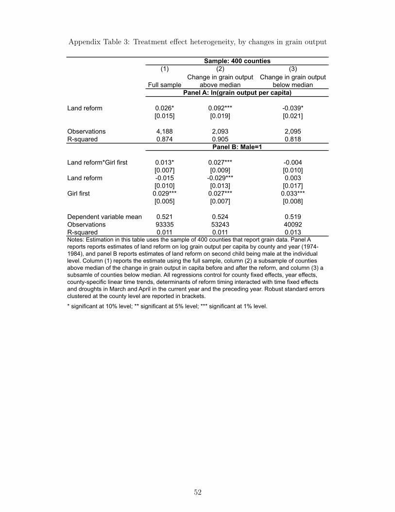
Appendix Table 3: Treatment effect heterogeneity, by changes in grain output
(1) (2) (3)
Full sampleChange in grain output
above medianChange in grain output
below median
Land reform 0.026* 0.092*** -0.039*[0.015] [0.019] [0.021]
Observations 4,188 2,093 2,095R-squared 0.874 0.905 0.818
Land reform*Girl first 0.013* 0.027*** -0.004[0.007] [0.009] [0.010]
Land reform -0.015 -0.029*** 0.003[0.010] [0.013] [0.017]
Girl first 0.029*** 0.027*** 0.033***[0.005] [0.007] [0.008]
Dependent variable mean 0.521 0.524 0.519Observations 93335 53243 40092R-squared 0.011 0.011 0.013
* significant at 10% level; ** significant at 5% level; *** significant at 1% level.
Panel B: Male=1
Panel A: ln(grain output per capita)
Sample: 400 counties
Notes: Estimation in this table uses the sample of 400 counties that report grain data. Panel A reports reports estimates of land reform on log grain output per capita by county and year (1974-1984), and panel B reports estimates of land reform on second child being male at the individual level. Column (1) reports the estimate using the full sample, column (2) a subsample of counties above median of the change in grain output in capita before and after the reform, and column (3) a subsamle of counties below median. All regressions control for county fixed effects, year effects, county-specific linear time trends, determinants of reform timing interacted with time fixed effects and droughts in March and April in the current year and the preceding year. Robust standard errors clustered at the county level are reported in brackets.
52

Appendix Table 4: County-level mean of male workers by crop in the 1982 Census
Obs Mean Std. Dev.A. county-leve mean of agricultural workers for each crop (all counties)Grain 1065 0.945 0.136Cash Crops 1065 0.050 0.132 Cotton 1065 0.033 0.126 Fruit 1065 0.002 0.011
B. county-level mean of male workers for each crop (counties that grow some particular crop)All Crops 1065 0.519 0.026Grain 1062 0.545 0.098Cash crops 935 0.515 0.227 Cotton 232 0.348 0.236 Fruit 407 0.692 0.331Notes: This table shows the summay statistics of county-level mean in the 1982 Census microdata. These counties can be matched with the county-level data on reform timing and the 1990 Census. The sample of individuals is restricted to agricultural workers. We use the unharmonized codes for occupation (OCC) and industry (IND) in the 1982 Census from IPUMS International to identify the crop an agricultural worker grows, e.g. fruit=1 if OCC==614&IND==14. We then obtain the county-level mean and report the mean and standard deviation across counties.
53

Appendix Table 5: Land size and gender
Total amount of cultivated land for household (mu=1/6 acre)
A. Chinese Health and Nutrition Survey 1989
% Male members 0.002[0.004]
Village FE X
dependent variable mean 3.1Observations 2495R-squared 0.438
B. Rural Fixed Point Survey 1986-1989 (Household-level Panel Data)
% Male labor 0.002[0.002]
dependent variable mean 7.6Observations 9,762No. of households 2,460R-squared 0.000Note: in Panel A, village fixed effects are controlled for. In Panel B, we report household fixed effect estimator using household-level panel data from 1986 to 1989.
54

Appendix Table 6: Extension of land lease in 1984
Male=1
Land reform*Girl first 0.030***[0.008]
Land reform -0.012*[0.007]
OCP*Girl first -0.003[0.008]
OCP -0.003[0.007]
1{Born in 1984-1986}*Girl first 0.013*[0.008]
Girl first 0.025***[0.003]
Observations 224600R-squared 0.011Notes: 1{Born in 1984-1986} is assigned 1 if one was born in 1984-1986 and 0 otherwise. The sample includes all second births between 1974 and 1986 in counties that are matched with the county-level data on timing of land reform and OCP. All regressions include county fixed effects, year of birth effects, county-specific linear trends, initial county controls interacted with birth year effects and droughts in March and April of the current year and the preceding year. * significant at 10% level; ** significant at 5% level; *** significant at 1% level.
55

Appendix Table 7: Heterogeneity by grain output in 1977
(1) (2) (3)
Full sampleGrain ouput in 1977
above medianGrain ouput in 1977
below median
Land reform*Girl first 0.017** 0.022** 0.011[0.007] [0.009] [0.011]
Land reform 0.002 -0.01 0.017[0.009] [0.012] [0.015]
Girl first 0.027*** 0.028*** 0.025***[0.005] [0.006] [0.007]
Observations 99024 52633 46162R-squared 0.011 0.011 0.011
Dependent variable: Male=1
* significant at 10% level; ** significant at 5% level; *** significant at 1% level.
Notes: Column 1 reports estimate for the effect of exposure to land reform on the probability of second child being male in the full sample; column 2 for the effect in counties above the median of grain output in 1977; column 3 for the effect in counties below the median. The sample includes individuals born between 1974 and 1986 in 400 counties that are matched with the county-level data on reform timing and grain output. All regressions include county fixed effects, year of birth effects, county-specific linear trends, initial county controls interacted with birth year effects and droughts in March and April of the current year and the preceding year. Robust standard errors clustered at the county level are reported in brackets.
56

Appendix Table 8: Land reform and infant health (UNICEF 1992 Chinese Children Survey)
Neonatal mortality Post-neonatal mortality Birth weightPanel A: All births
Land reform -0.0001 -0.003** 33.969**[0.002] [0.001] [15.320]
Observations 107934 107934 28876R-squared 0.015 0.019 0.158Panel B: Second births
Land reform*Girl first 0.002 -0.002 10.811[0.004] [0.003] [26.845]
Observations 31892 31892 8598R-squared 0.029 0.03 0.231
UNICEF 1992 Chinese Children Survey
* significant at 10% level; ** significant at 5% level; *** significant at 1% level.
Notes: Using the UNICEF 1992 Chinese Children Survey, we report estimated effects of land reform oninfant health outcomes. Panel A includes all births, and Panel B for the second births. All regressionsinclude county fixed effects, year of birth effects, county-specific linear trends, initial county controlsinteracted with birth year effects and droughts in March and April of the current year and the precedingyear. Robust standard errors clustered at the county level are reported in brackets.
57
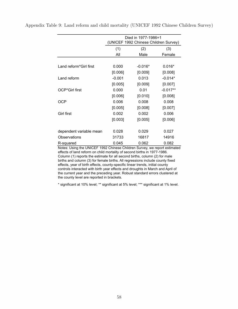
Appendix Table 9: Land reform and child mortality (UNICEF 1992 Chinese Children Survey)
(1) (2) (3)All Male Female
Land reform*Girl first 0.000 -0.016* 0.016*[0.006] [0.009] [0.008]
Land reform -0.001 0.013 -0.014*[0.005] [0.009] [0.007]
OCP*Girl first 0.000 0.01 -0.017**[0.006] [0.010] [0.008]
OCP 0.006 0.008 0.008[0.005] [0.008] [0.007]
Girl first 0.002 0.002 0.006[0.003] [0.005] [0.006]
dependent variable mean 0.028 0.029 0.027Observations 31733 16817 14916R-squared 0.045 0.062 0.082Notes: Using the UNICEF 1992 Chinese Children Survey, we report estimatedeffects of land reform on child mortality of second births in 1977-1986.Column (1) reports the estimate for all second births, column (2) for malebirths and column (3) for female births. All regressions include county fixedeffects, year of birth effects, county-specific linear trends, initial countycontrols interacted with birth year effects and droughts in March and April ofthe current year and the preceding year. Robust standard errors clustered atthe county level are reported in brackets.
* significant at 10% level; ** significant at 5% level; *** significant at 1% level.
Died in 1977-1986=1(UNICEF 1992 Chinese Children Survey)
58