Ple

ase

note

that

this

is a

n au

thor

-pro

duce

d P

DF

of a

n ar

ticle

acc

epte

d fo

r pub

licat

ion

follo

win

g pe

er re

view

. The

def

initi

ve p

ublis

her-a

uthe

ntic

ated

ver

sion

is a

vaila

ble

on th

e pu

blis

her W

eb s

ite

1

Canadian Journal of Fisheries & Aquatic Sciences 2007; 64(11): 1551–1562 http://dx.doi.org/10.1139/F07-123 © 2007 NRC Canada The original publication will be available at http://pubs.nrc-cnrc.gc.ca

Archimer http://www.ifremer.fr/docelec/

Archive Institutionnelle de l’Ifremer

Do survey design and wind conditions influence survey indices ?

Jean-Charles Poulard* and Verena M. Trenkel Ifremer, Department Ecology and Models for Fisheries, BP 21102, 44311 Nantes, France *: Corresponding author : Jean.Charles.Poulard@ifremer.fr

Abstract: Survey indices play an important role in stock assessments as they provide information on stock trends. In certain cases large interannual variations have been observed which are unlikely to reflect true underlying stock changes but are rather outliers. When survey indices for several species appear to be outliers for the same year, the suspicion is raised that something happened during the survey of that year. This is called a year-effect in survey catches. To study the potential year-effect in survey catches for the French autumn groundfish survey taking place in the Bay of Biscay, several indicators for survey design and wind conditions were derived as explanatory variables and Principal Component Analysis was used to study the relationship between these variables. Using multiple linear regression models we found that, on average 20% of interannual variation in abundance indices could be explained by survey conditions for benthic species, 11% for demersal and none for pelagic species. In contrast, survey conditions explained a smaller and decreasing part of the interannual variability in the coefficients of variations of these abundance indices and in species mean weight for benthic, demersal and pelagic species. Thus survey indices of benthic species seemed most affected by survey design and wind conditions. Keywords: survey index, catchability, time trends, survey conditions, Bay of Biscay.

Introduction

Abundance indices derived from scientific trawl surveys are used to inform on population trends

either directly, such as done by survey based assessment methods (Cook 1997; Korsbrekke et al. 2001) and the indicator approach to fisheries assessment (e.g. Trenkel and Rochet 2003), or indirectly through the tuning of stock assessment models (e.g. XSA, Shepherd 1999). The implicit assumption of such use of survey indices is that they reflect true trends in the underlying populations. In this context, interannual variability in an abundance index might be partly attributed to sampling variability and partly to true changes in population abundance. However, indices for a given year might be qualified as outliers if they seem too different from preceding and subsequent years to reflect true population changes, once stochastic population dynamics (e.g. recruitment) and sampling variability has been accounted for. Of course, the classification of outliers is mostly subjective. If the indices of several species appear to be outliers for the same year then this might suggest that something happened during the survey in that year. We refer to this effect as a year-effect in survey catches, whose main characteristics are that it affects many species simultaneously, appears on the spatial scale of the whole survey and is not caused by major changes in survey design or gear nor due to technical problems.

Strong year-effects in survey catchability affecting several species simultaneously were identified by Francis et al. (2003) when studying 17 trawl survey series around New Zealand. Pennington and Godø (1995), using VPA assessment results as a reference, estimated that the variability in survey indices due to annual variation in catchability was about double the within survey variability. The underlying mechanisms for these year-effects in catchability are not obvious as they have to be general enough to affect several species simultaneously. Environmental factors have been mentioned by Francis et al. (2003) as a possible explanation. Density-dependent effects might be another possibility (Swain et al. 1994).

Trawl catchability is commonly broken down into horizontal and vertical availability and gear efficiency. Horizontal availability, is the probability that an individual is found in the survey area while vertical availability is the probability that an individual is at the right distance from the bottom in order to be caught. Gear efficiency, defined as the probability that an individual that encounters the gear ends up in the catch, is determined by mesh size and reactions to the approaching gear (see Wardle 1993; Engås 1994 for reviews). All these probabilities can be influenced by environmental conditions but also local densities and population abundance in different ways for different species. However, in order to explain a year-effect in catchability, the different probabilities need to have been affected in a systematic manner by the environmental conditions occurring during the survey.

Horizontal availability is linked to the spatial distribution of species in relation to the area covered by the survey, which is generally fixed between years in most groundfish surveys. Both population density and environmental factors can lead to changes in the spatial distribution of a population and result in the population retracting outside the survey area (Fisher and Frank 2004). For example, Swain and Sinclair (1994) found that the area containing the majority of the cod population in the Southern Gulf of St. Lawrence increased with population abundance. In contrast, the area occupied by 0-group hake in the Bay of Biscay does not change with overall abundance due to strong habitat preferences (Petitgas 1998). Strong relationships between variations in density and local temperature, i.e. depth and latitudinal shifts, have been found for a wide range of species (Smith et al. 1991; Mountain and Murawski 1992; Albert et al. 2001). For example dab has been observed to move to deeper waters in years with higher temperatures (Bolle et al. 2001).

Vertical availability to bottom trawls can change on a regular basis due to diel migration behaviour. Differences between day and night catches have been reported from many areas for a variety of species (e.g. Casey and Myers 1998; Petrakis et al. 2001; Benoît and Swain 2003). Short term changes in vertical distributions have been explained by variations in water turbidity following storm events, as observed for the flatfishes dab, sole and plaice and the pelagic species mackerel and horse-mackerel (Ehrich and Stransky 1999). Alternatively, turbidity might alter reaction behaviours and thus modify trawl efficiency. Changes in the vertical distribution might also be a consequence of current conditions influencing individual fish activity, as has been observed for some deep-sea fish species (Lorance and Trenkel 2006). Trawl efficiency, as a result of changes in trawl geometry, has been found to depend on water depth, current speed and direction (see review by Engås 1994). Individual reaction behaviour is found to increase with visibility (Bolle et al. 2001) and to be modified by temperature, with higher temperatures leading to stronger avoidance reactions for some deep-sea species (Lorance and Trenkel 2006) but higher catchability for American lobster due to temperature related activity patterns (Drinkwater et al.

2

2006). Changes in temperature can be brought about by the impact of wind conditions on temperature via the creation of upwelling events (Drinkwater et al. 2006). Wind can also influence bottom currents and subsequently individual behaviour, as put forward as explanation for the observation that catch rates of plaice off Lowestoft seem to depend on wind direction (Harden and Scholes 1980). Wind conditions are also expected to influence trawl efficiency directly through its effect on ship motion (Bolle et al. 2001) and trawl geometry.

In this paper we investigate the existence of a year-effect in survey catchability and its impact on survey indices for the Bay of Biscay groundfish community using Western International Bottom Trawl Survey (WIBTS) data for the years 1987 to 2003. The survey indices studied are species density estimates, the coefficient of variation of these density estimates as well as species mean weight. Species density and mean weight indices are increasingly used as indicators for population health (e.g. Trenkel and Rochet 2003). Interannual variability in survey catchability is modelled using variables describing survey design and survey conditions. The possible impact of changes in survey design need to be investigated, as unfortunately some small but possibly influential changes in survey starting dates and number of hauls have occurred over the course of the survey series. In order to account for species-specific effects, we investigate catchability year-effects by life style group, thus we consider separate effects for benthic, demersal and pelagic species. The division into these three groups is expected to encapsulate species differences in catchability, mainly vertical availability and gear efficiency. Species-specific effects could only be studied on the individual haul level, but not on the level of annual survey indices, for the obvious reason that there is only one survey index estimate per year. Previous work (Poulard et al. 2003) has shown the relative temporal stability of the spatial fish community organization in the Bay of Biscay. Therefore, unless temperature conditions make a particular species move out of the survey area (horizontally or vertically), no effect of temperature on survey indices used in this study on the large scale of the survey is expected. Thus temperature is not considered as an explanatory factor. The issue might be different on the haul level, as temperature conditions have been observed to influence local species densities (Smith et al., 1991; Mountain and Murawski 1992; Albert et al. 2001). On the other hand, a main characteristic of the hydrography on the Bay of Biscay shelf is the relatively rapid response of shelf waters to permanent wind stress (Puillat et al. 2004). Consequently, considering prevailing wind conditions seems to be a suitable way to study the effects of survey conditions (physical effects on gear, effects of current and mesoscale hydrodynamic features) on the interannual variability of survey indices.

The main questions examined are: What factors influence annual survey catchability? What proportion of interannual variability in survey derived indicators can be explained by a year-effect in survey catchability? For this, first a multivariate analysis is performed to identify and summarize the main changes which occurred in survey design and wind condition indicators during the study period. Second, for a selection of survey design and wind condition indicators, their explanatory power for each of three survey indices is studied using multiple regression. This allows the identification of the factors influencing annual survey catchability and the quantification of the interannual variability in survey indices explainable by those factors.

3

Material and methods

Survey data

Data were collected during 14 groundfish surveys carried out by IFREMER from October to December between 1987 and 2003 (EVHOE series with gaps in 1991, 1993 and 1996), on the eastern continental shelf of the Bay of Biscay (ICES 1997; Poulard et al. 2003; Poulard and Blanchard 2005). The study area is situated between 43º30'N and 48º30'N and depth ranges from 15 to 600 m (Figure 1). The sampling design was stratified according to latitude and depth. A 36/47 GOV trawl was used with a 20 mm mesh codend liner. Haul duration was 30 minutes at a towing speed of 4 knots. Fishing was mainly restricted to daylight hours. Catch weights and catch numbers were recorded for all species. A total of 200 fish species were caught but only 40 fish species, present on average in at least 10% of the tows with a density of at least 5 fish per km2, were included in the analysis (see Appendix A). Wind direction and wind speed were recorded during trawling. The number of hauls per year varied from 70 to 135. Overall 1406 hauls were analysed. The survey vessel changed in 1997 from Thalassa 1 to Thalassa.

Variables

Survey condition indicators Wind indicators were prepared in the following way for each survey. First the polar coordinates

of the wind vector were transformed to Cartesian coordinates, then the average half-daily wind vectors were computed. The plot of the vector sum of these half-daily wind vectors gives the hodograph (Figure 2). The hodograph is a simple way to summarise the evolution of the wind during each survey. From it, we derived five wind indicators (Table 1 and Figure 3). The length of the mean half-daily wind vector (MDWV, Figure 3a) measures the average wind strength during the survey and the standard deviation of MDWV (MDWV.std, Figure 3a) measures its irregularity while its coefficient of variation (MDWV.cv, Figure 3b) expresses the relationship between average wind strength and its variability.

The persistence of the wind direction is captured by Wpers ( BArr

/ , Figure 3b); it takes a value of 1 if

the wind has always been blowing from the same direction during the whole survey and close to zero if it has been changing direction all the time. WD (Figure 3c) is simply the average wind direction.

Five survey design indicators (Table 1) were derived to describe changes which occurred in the survey design. They are the mean sample area of influence, the latitude and longitude of the centre of gravity of haul positions, the survey starting day (Julian day) and the number of hauls in the two most shallow sampling strata (<80 m, see Figure 1).

The mean sample area of influence (MSAI, Figure 3d) encapsulates information on sampling effort and the spatial distribution of hauls. The estimation of the area of influence of each sample (haul) proceeds as follows: overlay a fine regular grid on the survey area, determine which sampling location is closest to each grid cell then for each sampling location count the number of times it is the closest. The average of these counts gives the mean sample area of influence for a given survey. Note that the survey area needs to be identical for all years. The value of the MSAI depends on the distance between neighbouring hauls. It is inversely proportional to sampling effort and is also an indicator of spatial regularity in survey coverage.

Sampling effort (number of hauls) decreased during the study period and unfortunately the decrease was not homogenous across all strata but was relatively more severe in shallower strata (< 80 m). So, we defined the number of hauls close to the coast (NHC, Figure 3d) as an indicator.

The Julian day of the starting date of each survey was taken as an indicator (start, Figure 3e). The earliest survey started September 18 (Day 262) in 1992 while the latest started November 11 (Day 315) in 1999. The first six surveys tended to start earlier. When the research vessel was changed in 1997, the starting date of the survey was delayed and subsequently survey starting dates gradually moved towards later dates.

The spatial distribution of the centres of the gravity of the hauls (Figure 3f) was very stable in latitude (the latitude range was 44 km) and more variable in longitude (the longitude range was 70 km) due to the geometry of the study area. Species survey indices

For 40 selected fish species, total and mean density and total biomass in the survey area as well as their sampling precisions were computed using the swept area method and accounting for the stratified sampling design. Based on this information, the following indices were calculated for each

4

species and year: mean density normalised per species ((density – mean density)/standard deviation), DENS; normalised coefficients of variation of species density, CV; and normalised mean individual weight (total abundance divided by total biomass), Wbar (Figure 4). Density estimates in 1994 and 1995 were relatively high for most species of all life style groups; for benthic (17) and demersal (16) species estimates for 2001 were high compared to the preceding year and those 2003 (Figure 4 top). CVs of density estimates seemed to have been particularly low for many benthic species in 2002 and rather high in 1999 (Figure 4 centre). For pelagic (7) and benthic species, mean individual weight was higher at the beginning of the series in 1989-1990, compared to the mid nineties (Figure 4 bottom).

Analysis

Principal Component Analysis (PCA) was used to study the relationships between variables in the table of survey design and wind indicators.

Relationships between the three sets of species survey indices (density, CV of density estimates and mean weight) and survey design and wind indicators were then investigated by multiple regression. All indices were normalised for each species separately, in order to allow across species analysis without any species dominating the results. The PCA results were used to identify four explanatory variables that potentially carried independent information: the norm of the mean and the standard deviation of the half-daily wind vectors (MDWV and MDWV.std), the number of hauls close to coast (NHC), and survey starting date (start). As the time series for MDWV and start were positively correlated (p<0.001), an interaction term was also fitted when ever both variables appeared in a model. To these four variables were added factors for the survey vessel (R/V Thalassa 1 before 1997 and Thalassa thereafter) and the species life style (benthic, demersal or pelagic, see Appendix A for species list). The impact of the changes in survey design and wind conditions on trawl catchability, and consequently on survey indices, is expected to be different according to the species life style, abbreviated as LS.

The LS variable was not used as an explanatory variable as such, but it was tested whether a different relationship (slope) applied for each life style group. For this test, single variable models were fitted for the selected five survey condition variables and compared to models with different relationships for each live style group. This was achieved by fitting models which contained only the interaction term between each variable and the life style variable. The comparison was carried out using Akaike's information criterion (AIC). In the further analysis, if the model with different relationships for each life style group had the better fit, it was used whenever the variable occurred in a model, i.e. a LS-variable interaction was fitted. Otherwise a common relationship for all species was assumed. The full model including all five explanatory variables and all subset models with only main effects (exception start-wind strength interaction) were fitted, amounting to 36 models. Model selection and comparison were carried out using the information theoretic approach (Burnham and Anderson 2002). For this the AIC difference Δ between the AIC for the best model (smallest AIC) and all other models was calculated. Thus for model i,

AICi = - 2 logLiki + 2k Δi = AICi – AICmin

where logLik is the log likelihood and k the number of parameters of model i (number of variables + 1 for intercept + 1 for variance of error distribution). Burnham and Anderson (2002) gave the rule of thumb that models with Δi up to 2 are taken to be equivalent with the best model and for Δi up to 7 there is substantial support for the model in the data. Akaike weights wi were calculated as a measure of the evidence that model i is supported by the data.

( ) ( )∑=

Δ−Δ−=36

1 21exp/2

1expr

riiw .

The sum of these Akaike weights for the models where a given explanatory variable j was

present, denoted as w+(j), allowed to measure the relative importance of each explanatory variable. A large w+(j) indicates that variable j is relatively important. We then investigated the achievable explanation in the interannual variability in survey indices based on the best model using the coefficient of determination R2 (i.e., 1-(residual sums of squares/total sums of squares)). Finally, linear time trends in survey density and mean weight were estimated by species and compared to linear time trends obtained when survey conditions had been accounted for using the best model in each case.

5

Results

Analysis of survey design and wind indicators

The first two axes of the PCA accounted for 78 % of the total variance. The remaining components were too weakly explained by variables or too noisy to be useful for describing the data set. Some indicators were highly correlated with the first axis (Figure 5, Table 1, PCA axes). Based on the first principal component axis, the 14 survey years can be grouped into two periods, from 1987 to 1994 and from 1995 to 2003 (Figure 6).

The norm of the mean half-daily wind vector (MDWV) was negatively correlated with the first axis while its coefficient of variation (MDWV.cv) was positively correlated. This means wind strength increased and became relatively more regular in the course of the survey series (Figure 3a).

The starting date (start) increased in the same way (Figure 3e). The difference between the earliest survey (1992) and the latest (1999) was 53 days, but two periods can be identified. Until 1994 the mean starting date was Julian day 270 and varied little, whilst during the second period the mean starting date was 295 with two very late starting dates (more than 310) in 1995 and 1999.

Changes in sampling effort were also taken into account by the first principal component axis. The number of hauls close to the coast decreased from right to left along the first axis (Figure 5, Table 1, PCA axes) while the mean sample area of influence (MSAI) changed in the opposite direction. There was some redundancy between these two indicators.

The average survey longitude and the wind direction contributed little to the first axis. The centres of gravity of the early surveys (1987 to 1994) were closer to the coast (Figure 3f) because the number of hauls in shallow water was higher. However, in 1995 a few more hauls were made at greater depths in the north of the study area. Southerly and especially westerly winds have been prevailing during the second survey period while the wind direction was rather variable during the first one (Figure 3c).

The two different measures of wind persistence (Wpers for direction and MDWV.std for strength) were negatively correlated with the second principal component axis (Figure 5, Table 1). Wind strength has been more variable in years located in the area associated with the negative part of the second axis in Figure 5, in some of these years (i.e. 1992, 1998 and 2000) the persistence of the wind direction was also high.

The correlation of the average survey latitude and longitude with the second axis is explained by the greater variability in the spatial distribution of the centres of gravity of the surveys during the second period of the survey series. The deeper strata (400-600 m) were not sampled in 1997 and 1998, so the centres of gravity were located more to the east. After 1998, the centre of gravity of survey hauls moved to the west and north.

Relating species survey indices to survey design and wind conditions

Single variable analysis showed that wind strength (MDWV) was the single best explanatory variable as it has the smallest AIC for all three survey indices (Table 2). The second best variable differed between survey indices. Models assuming a different relationship for each life style generally had a worse fit than models taking into account a common relationship for all life styles (see Table 2 and compare models 1 to 5 with respectively models 6 to 10). The notable exception was the vessel effect, which varied between species life style groups for survey density estimates but neither for the CV of survey densities nor for mean weight. Fewer benthic fish and demersal fish seemed to be caught by the new research vessel Thalassa. Thus, all the results regarding survey densities models have been computed with a separate vessel effect for each species life style group.

The best model for normalised survey density estimates included all five explanatory variables (model 11 in Table 3a). Note that only models within 7 units of the minimum AIC are reported. The importance of these five explanatory variables was reflected by evidence weights close to one (Table 4). Survey densities decreased with more hauls close to the coast (NHC) and with larger wind variability during the survey (MDWV.std) (Table 4). These signs are based on the best model (Table 3). The signs for the main effects of wind strength (MDWV) and starting date (start) cannot be interpreted due to the interaction term included in the model. The observed vessel effect reflects that the old vessel gave higher densities compared to the new one for demersal and pelagic species.

There was no clear best model for the CV of density estimates. The model with the smallest AIC (model 25 in Table 3b) included survey starting date (start) and wind speed (MDWV), plus the interaction term, and wind variability (MDWV.std). Other models including vessel effect were nearly as good. The evidence weights however suggested that starting date and wind speed and wind strength

6

variability were the most important variables for explaining the CV of survey density estimates (Table 4). Higher wind variability lead to higher CVs (positive relationship).

For normalised mean weight, the model including starting date, mean wind strength and variability had the smallest AIC, but the AIC for a range of other models was nearly identical (Table 3c). Evidence weights suggested that indeed these three variables were the most important ones for explaining mean weight (Table 4). Mean weight decreased at higher wind variability (MDWV.std).

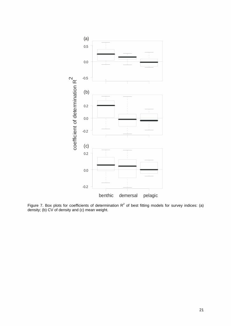
The proportion of interannual variation in survey indices that might be explained by survey design and wind conditions was obtained by calculating the coefficient of variation R2 of the best fitting models (Figure 7). For survey density estimates, the R2 was highest for benthic and demersal species, with an average R2 of 0.2 and 0.11 respectively which concerned a large majority of species. The average R2 for pelagic species was 0, with about half the species having positive and negative values. For the CV of density estimates, the highest R2 was again achieved for benthic species, with an average of 0.15. For demersal and pelagic species negative R2 values were found in most cases. The results were even less strong for mean weight. Again benthic species were most affected by the reduction in interannual variance, with an average R2 of 0.6; for demersal species the average was 0.3 and 0.2 for pelagic species. Thus survey and wind condition indicators were most effective in explaining interannual variability of survey density estimates, then the CV of those estimates and not much mean weight. Benthic species followed by demersal species were most affected.

The comparison between linear time trends in raw survey indices and model residuals allows to assess whether spurious time trends might have been introduced by changing survey and wind conditions. Significantly increasing densities (p-value ≤ 0.05) were found for 11 species, while densities decreased over time for two. Taking into account all five explanatory variables (best model), significant positive time trends were found for five additional species. In contrast, increasing trends were no longer significant for eight species and one decreasing trend for one species. The species concerned by the change belonged to all three life style groups. Thus taking account of survey conditions meant that eight instead of 11 species were found to increase over the time series and only one instead of two decreased. Mean weight decreased significantly during the study period for eight species. Taking into account explanatory survey variables meant that a different set of eight species had significantly decreasing weights.

Discussion

A non-negligible proportion of interannual variability in survey density estimates and to some degree in the precision of density estimates could be explained by changes in survey design and wind conditions prevailing during the survey. Benthic species were more sensitive than demersal species, while pelagic species did not seem to be concerned. Thus year-effects in survey indices which might indicate year-effects in catchability seem to be present in the Western IBTS survey series. Average wind strength during the survey period was the single most important explanatory variable, but also wind variability, survey starting date, the number of coastal hauls and the change in survey vessel contributed to explain interannual variability in density estimates. For benthic species the year-effect of catchability was estimated to account for 20% of interannual variability on average, while it was 11% for demersal species. This agrees well with the findings by Bolle et al. (2001), who explained 2-7% of interannual variance in survey density estimates for dab by wind stress, temperature and turbidity variations.

The information theoretic approach chosen here allows to assess the relative importance of different explanatory variables. However, this does not mean that there is any causal link. Indeed, the fact that survey design and wind conditions have changed simultaneously, renders the search for causality with this data set futile. Both gradual and sudden changes through time were exhibited by most of the survey design and wind conditions indicators, especially in survey starting dates and deployment of sampling effort. It seems that as a consequence of surveys starting later in the year, different wind conditions were observed. Thus the effects of stronger winds and later starting were confounded and hence cannot be interpreted separately. The combined chronology of the different observed changes led to identify two distinct periods: from 1987 to 1994 and from 1995 to 2003. The first period was dominated by more stable survey conditions, while the second period was characterised by more variability in some indicators like wind direction and strength, sampling effort and survey starting day. Without being a true outlier, the location of the year 1999 on the first PCA axis (Figure 6) and its important contribution to the construction of this axis have to be noted. In 1999, the survey started very late due to the Erika oil spill and the sampling effort was the lowest during the series as the area around the oil spill could not be sampled. Incidentally this division into two periods

7

also nearly corresponds to the change in survey research vessel which occurred in 1997. There was no survey in 1996 and the first survey with the new vessel was carried out in 1997. Poulard and Blanchard (2005) in using correspondence analysis for nearly the same species density data also identified two periods: 1973 to 1995 and 1997 to 2002. The periods were characterised by two groups of species exhibiting opposite abundance trends. Here linear time trends in density estimates were shown to be rather sensitive to year-effects in catchability. This effect might have been exacerbated by the relative shortness of the time series (14 surveys for 17 years). Nicholson and Jennings (2004) have already noted the low power of fisheries surveys to detect linear time trends in survey indicators, in their case they investigated community indicators.

A life style dependent vessel effect was found in this study. It seems that the new research vessel Thalassa is less efficient than the old one in catching benthic and demersal species. In an intercalibration study, significantly lower catches were recorded for the new vessel for eight out of 21 species-size groups (Pelletier 1998). Significant higher catches were only found for two species (one benthic and one demersal). Our study seems to confirm these findings.

In general, the degree of interannual variability explained by survey indices and survey condition variables was highest for benthic species, less for demersal and absent for pelagic species and concerned mainly density estimates. This result does not come as a surprise. Several mechanisms can explain why the relationship between density estimates and wind conditions should be strongest for benthic species. This is less obvious for survey design changes. Later starting dates are expected to affect gear efficiency (due to selectivity effects) for newly recruited fish for all species spawning at the beginning of the year as recruits have more time to grow. The large majority of species considered in this study spawn during the first half of the year; the species belong to all life style groups. A similar seasonality effect has been observed for commercial catch yields for trawlers operating in the Bay of Biscay (Poulard and Léauté 2002). For species carrying out diurnal migrations, the fact that day time is shorter later in the year might also play a role, despite fishing mainly being restricted to daylight hours. A rich literature exists describing the variations in bottom trawl catches as a function of day light (e.g. Casey and Myers 1998). Casey and Myers found that while migrating species were generally caught in higher numbers during the day, it was the opposite for species relying on visual cues for avoiding the trawl. However, benthic species do no usually carry out diurnal migrations and should therefore not be concerned by changes in daylight duration during the survey. It is not evident what mechanisms could be responsible for estimated densities being lower in surveys with more hauls close to the coast. The opposite might have been explained by a better coverage of coastal nursery areas. So this result might reflect some other not modelled covariate. It has been shown (Poulard et al. 2003) that depth is an important structuring factor for the spatial organization of the fish assemblages on the eastern continental shelf of the Bay of Biscay.

Wind strength and wind variability were only weakly related (R2=0.20), so that the increase in wind strength variability in some years can be mainly interpreted as the succession of quiet weather and short term blasts. These changeable weather conditions probably impacted gear efficiency. It seems plausible that benthic, but also demersal species should be more concerned by variations in gear efficiency. For pelagic species wind impact is more likely to affect vertical availability. In years with strong wind variability, species densities had a tendency to be underestimated and to have lower estimation precision (higher CV). A sign of reduced gear efficiency might also be the result that individual mean weight was general lower in years with higher wind variability.

Taking into account survey design and wind conditions did not so much modify the number of species with significant time trends in population density or mean weight, but the identity of those species. Thus the community wide perception of time trends was not affected, hence this data can be used for assessing the status of the Bay of Biscay exploited fish community as done by Rochet et al. (2005). However care has to be taken when interpreting trends for individual species.

Overall, we have been looking for a year-effect in catchability which would impact many species simultaneously and could be detected by common relationships with explanatory variables. In accordance to prior expectations, benthic species were found to be more concerned than demersal species and even more so than pelagic species. Of course, the crude classification of species into life style groups does not capture all species-specific behaviour differences. More detailed analyses by species would be required in order to study specific effects. However, the species-specific effects were reflected in the range of the percentages of interannual variability in survey indices explained by survey conditions.

In conclusion, our study shows that interannual variations in density estimates might have been amplified by changes in survey conditions and their precision somewhat degraded, in particular for benthic species. The simultaneous time drift that occurred in several survey conditions, both related to the survey design and the environment, makes it difficult to definitely conclude causal links between

8

survey conditions and species survey indices. However, it seems that even minor adjustments in survey design, justified as they might be in the particular case, can jeopardise the integrity of a survey series and hamper the move towards survey based fish and community assessments in the context of an ecosystem approach to fisheries management.

Acknowledgment

We wish to thank J.-C. Mahé who is in charge of the EVHOE surveys and all our colleagues involved in the data collection. This study was partially funded by the EU project FISBOAT (Fisheries Independent Survey Based Operational Assessment Tools), contract number 502572.

9

References

Albert, O.T., Nilssen, E.M., Nedreaas, K.H., and Gundersen, A.C. 2001. Distribution and abundance of juvenile Northeast Arctic Greenland halibut (Reinhardtius hippoglossoides) in relation to survey coverage and the physical environment. ICES J. Mar. Sci. 58: 1053-1062.

Benoît, H.P. and Swain, D.P. 2003. Accounting for length- and depth-dependent diel variation in catchability of fish and invertebrates in an annual bottom-trawl survey. ICES J. Mar. Sci. 60: 1298-1317.

Bolle, L.J., Rijnsdorp, A., and Van Der Veer, H.W. 2001. Recruitment variability in dab (Limanda limanda) in the southeastern North Sea. J. Sea Res. 45: 255-270.

Burnham, K.P., and Anderson, D.R. 2002. Model selection and multimodel inference. A practical Information-theoretic approach. Second edition. Springer, New York.

Casey, J., and Myers, R.A. 1998. Diel variations in trawl catchability: is it as clear as day and night? Can. J. Fish. Aquat. Sci. 55: 2329-2340.

Cook, R.M. 1997. Stock trends in six North Sea stocks as revealed by an analysis of research vessel surveys. ICES J. Mar. Sci. 54: 924-933.

Drinkwater, K.F., Tremblay, M.J., and Comeau, M. 2006. The influence of wind and temperature on the catch rate of the American lobster (Homarus americanus) during spring fisheries off eastern Canada. Fish. Oceanogr. 15: 150-165.

Ehrich, S., and Stransky, C. 1999. Fishing effects in northeast Atlantic shelf seas: patterns in fishing effort, diversity and community structure. VI. Gale effects on vertical distribution and structure of a fish assemblage in the North Sea. Fish. Res. 40: 185-193.

Engås, A. 1994. The effects of trawl performance and fish behaviour on the catching efficiency of demersal sampling trawls. In Marine fish behaviour in capture and abundance estimation, Edited by A. Fernö and S. Olsen. Fishing News Books, Oxford, pp. 45-68.

Fisher, J.A.D., and Frank, K.T. 2004. Abundance-distribution relationships and conservation of exploited marine fishes. Mar. Ecol. Prog. Ser. 279: 201-213.

Francis, R.I.C.C., Hurst, R.J., and Renwick, J.A. 2003. Quantifying annual variation in catchability for commercial and research fishing. Fish. Bull. 101: 293-304.

Harden Jones, F. and Scholes, P. 1980. Wind and the catch of a Lowestoft trawler. J. Cons. int. Explor. Mer 39: 53-69.

ICES. 1997. Report of the International Bottom Trawl Survey Working Group. CM 1997/H:6, 50 pp. Korsbrekke, K., Mehl, S., Nakken, O., and Pennington, M. 2001. A survey-based assessment of the

Northeast Arctic cod stock. ICES J. Mar. Sci. 58: 763-769. Lorance, P., and Trenkel, V.M. 2006. Variability in natural behaviour, and observed reactions to an

ROV, by mid-slope fish species. J. Exp. Mar. Biol. Ecol. 332: 106-119. Mountain, D.G., and Murawski, S.A. 1992. Variation in the distribution of fish stocks on the northeast

continental shelf in relation to their environment, 1980-1989. ICES Mar. Sci. Symp. 195: 424-423. Nicholson, M.D., and Jennings, S. 2004. Testing candidate indicators to support ecosystem-based

management: the power of monitoring surveys to detect temporal trends in fish community metrics. ICES J. Mar. Sci. 61: 35-42.

Pelletier, D. 1998. Intercalibration of research survey vessels in fisheries: a review and an application. Can. J. Fish. Aquat. Sci. 55: 2672-2690.

Pennington, M. and Godø, O.R. 1995. Measuring the effect of changes in catchability on the variance of marine survey abundance indices. Fish. Res. 23: 301-310.

Petitgas, P. 1998. Biomass-dependent dynamics of fish spatial distributions characterized by geostatiscal aggregation curves. ICES J. Mar. Sci., 55: 443-453.

Petrakis, G., MacLennan, D.N., and Newton, A.W. 2001. Day-night effects on catch rates during trawl surveys in the North Sea. ICES J. Mar. Sci. 58: 50-60.

Poulard, J.-C., Blanchard, F., Boucher, J., and Souissi, S. 2003. Variability in the demersal fish assemblages of the Bay of Biscay during the 1990s. ICES Mar. Sci. Symp. 219: 411-414.

Poulard, J.-C., and Blanchard, F. 2005. The impact of climate change on the fish community structure of the eastern continental shelf of the Bay of Biscay. ICES J. Mar. Sci. 62: 1436-1443.

Poulard, J.-C. and Léauté, J.-P. 2002. Interaction between marine populations and fishing activities: temporal patterns of landings of La Rochelle trawlers in the Bay of Biscay. Aquat. Living Resour. 15: 197-210.

Puillat, I., Lazure, P., Jégou, A.-M., Lampert, L., and Miller, P.I. 2004. Hydrographical variability on the French continental shelf in the Bay of Biscay, during the 1990s. Cont. Shelf Res. 24: 1143-1163.

Rochet, M.-J., Trenkel, V.M., Bellail, R., Coppin, F., Le Pape, O., Mahé, J.-C., Morin, J., Poulard, J.-C., Schlaich, I., Souplet, A., Vérin, Y., and Bertrand, J. 2005. Combining indicator trends to assess

10

ongoing changes in exploited fish communities: diagnostic of communities off the coasts of France. ICES J. Mar. Sci. 62: 1647-1664.

Shepherd, J.G. 1999. Extended survivors analysis: An improved method for the analysis of catch-at-age data and abundance indices. ICES J. Mar. Sci. 56: 584-591.

Smith, J.J., Perry, R.I., and Fanning, L.P. 1991. Relationships between water mass characteristics and estimates of fish population abundance from trawl surveys. Environ. Monit. Assess. 17: 227-245.

Swain, D.P., Nielsen, G.A., Sinclair, A.F., and Chouinard, G.A. 1994. Changes in catchability of Atlantic cod (Gadus morhua) to an otter-trawl fishery and research survey in the southern Gulf of St Lawrence. ICES J. Mar. Sci. 51: 493-504.

Swain, D.P., and Sinclair, A.F. 1994. Fish distribution and catchability: What is the appropriate measure of distribution? Can. J. Fish. Aquat. Sci. 51: 1046-1054.

Trenkel, V.M., and Rochet, M.-J. 2003. Performance of indicators derived from abundance estimates for detecting the impact of fishing on a fish community. Can. J. Fish. Aquat. Sci. 60: 67-85.

Wardle, C. S. 1993. Fish behaviour and fishing gear. In Behaviour of teleost fishes. Edited by Pitcher, T. J., Chapman & Hall, London, 609-643pp.

11

Table 1. List of the selected wind and survey design indicators and their basic statistics. Correlation between these indicators and the first two Principal Component Analysis (PCA) axes.

PCA axesIndicator types

Variable Code Mean Minimum Maximum 1 2

Norm of the mean daily wind vector (m•s-1)

MDWV 8.36 4.72 11.90 -0.9 -0.3

MDWV Standard deviation (m•s-1) MDWV.std 4.06 3.20 5.50 -0.2 -0.9Wind MDWV coefficient of variation MDWV.cv 0.51 0.36 0.73 0.9 -0.2 Persistence WPers 0.36 0.09 0.66 -0.1 -0.7 Direction (polar coordinates) WD 128.71 5.00 354.00 0.5 0.4 Mean sample area of influence (km2) MSAI 10.75 7.55 14.99 -0.8 -0.4 Number of hauls close to coast NHC 23.36 9.00 35.00 0.9 0.0Survey design

Average survey latitude (° N) Lat 46.35 46.13 46.53 -0.2 1.0

Average survey longitude (° W) Long -3.78 -4.26 -3.34 0.5 -0.8 Survey starting day (Julian day) start 284.14 262.00 315.00 -0.9 0.2

Table 2. Summary of model fits for mono-variable linear models. In models 1 to 5, the same relationship is assumed for the all species life styles. In models 6 to 10 (variable:type), different relationships per species life type are assumed. Variable names are listed Table 1. LogLik: log likelihood; AIC: Akaike information criteria; Δ = AIC - min(AIC) for models in table.

Density CV Mean weight Model Variables df

LogLik AIC Δ LogLik AIC Δ LogLik AIC Δ

1 start 3 -766.7 1539.4 15.7 -771.0 1547.9 0.2 -773.3 1552.6 11.3

2 NHC 3 -766.7 1543.4 19.7 -771.6 1549.2 1.5 -769.2 1544.3 3.0

3 MDWV 3 -758.9 1523.7 0 -770.8 1547.7 0 -767.7 1541.3 0

4 MDWV.std 3 -758.3 1526.7 3.0 -771.1 1548.2 0.5 -773.4 1552.7 11.4

5 Vessel 3 -765.7 1537.4 13.7 -771.4 1548.8 1.1 -769.1 1544.1 2.8

6 start:type 5 -765.6 1541.2 17.5 -771.0 1551.9 4.2 -773.3 1556.5 15.2

7 NHC:type 5 -771.8 1549.6 25.9 -771.1 1552.1 4.4 -769.1 1548.2 6.9

8 MDWV:type 5 -771.8 1553.6 29.9 -770.5 1550.9 3.2 -767.5 1545.1 3.8

9 MDWV.std:type 5 -764.1 1534.1 10.4 -771.0 1552.0 4.3 -773.3 1556.7 15.4

10 vessel:type 7 -759.3 1532.6 8.9 -767.9 1549.7 2.0 -768.2 1550.3 9.0

12

Table 3. Summary of fits for multi-variable linear models for: a) density b) CV of density and c) mean weight. Variable names are listed Table 1. LogLik = log likelihood; AIC = Akaike information criteria; Δ = AIC - min(AIC). Models are only shown when Δ is less than 7 (Δ<7), they are sorted by Δ ascending order. The vessel effect used was different according the species life style (benthic, demersal and pelagic) for the species density estimates.

a) Density

Model Variables df LogLik AIC Δ11 all variables 12 -734.8 15493.7 0

b) CV of density estimates

Model Variables df LogLik AIC Δ 25 start*MDWV, MDWV.std 6 -758.9 1529.7 032 start*MDWV, MDWV.std, vessel 7 -758.7 1531.4 1.730 start*MDWV, NHC, MDWV.std 7 -758.8 1531.7 1.911 all variables 8 -758.7 1533.3 3.613 start*MDWV 5 -762.0 1534.1 4.422 start* MDWV, NHC 6 -762.0 1536.1 6.4

c) Mean weight

Model Variables df LogLik AIC Δ 25 start*MDWV, MDW.std 6 -762.6 1537.3 030 start*MDWV, NHC, MDWstd 7 -761.9 1537.9 0.632 start* MDW, vessel, MDW.std 7 -762.5 1539.0 1.711 all variables 8 -761.7 1539.3 2.03 MDWV 3 -767.7 1541.3 4.113 start*MDWV 5 -766.1 1542.3 5.022 start*MDWV, NHC 6 -765.3 1542.6 5.319 MDWV, MDW.std 4 -767.4 1542.7 5.416 NHC, MDWV 4 -767.4 1542.8 5.520 MDW, vessel 4 -767.5 1543.0 5.735 start*MDWV, vessel 6 -765.9 1543.8 6.65 vessel 3 -769.1 1544.1 6.933 start*MDWV, NHC, vessel 7 -765.0 1544.1 6.82 NHC 3 -769.2 1544.3 7.0

13

Table 4. Evidence weights w+ based on the 36 models fitted for each explanatory variable (variable names are listed Table 1). Sign of the linear relationship for the best fitting model (smallest AIC in Table 3). Vessel: Th1 = Research Vessel Thalassa 1 (before 1997) and Th = R/V Thalassa (from 1997). The vessel effect used was different according to the species life style (b benthic, d demersal and p pelagic) for the species density estimates.

Evidence weights w+ Sign of linear relationship Variable Density CV Mean weight Density CV Mean weight

start 1.00 1.00 0.84 + - - MDWV 1.00 1.00 0.95 + - - NHC 0.98 0.28 0.43 - 0 0 MDWV.std 1.00 0.92 0.81 - + - vessel 0.98 0.28 0.32 Th < Th1 d & p 0 0

14

44°N

10°W 9°W 8°W 7°W 6°W 5°W 4°W 3°W 2°W

45°N

46°N

47°N

48°N

Figure 1. Area of the eastern continental shelf of the Bay of Biscay studied during the 14 groundfish surveys carried out by Ifremer from September to December from 1987 to 1990, in 1992, 1994, 1995 and from 1997 to 2003.

15

Half daily wind vector

Survey start

B = sum of the norm of half daily wind vector

A = vectorial sum ofhalf daily wind vector

400

400

200

200

0

0

-200

-200

v

u

Figure 2. Details of the construction of the wind hodograph and definition of the A and B vectors.

16

0.0

0.1

0.2

0.3

0.4

0.5

0.6

0.7

0.8

1987 1990 1993 1996 1999 2002Year

0

5

10

15

20

25

30

35

40

1987 1990 1993 1996 1999 2002Year

Num

bero

fhau

ls

0

2

4

6

8

10

12

14

16

Surfa

ce(k

m2)

1997

1992

1987

2003

1994

2002

1999

2001

1995

46.1

46.2

46.3

46.4

46.5

46.6

-4.50 -4.00 -3.50 -3.00Longitude (°W)

Latit

ude

(°N

)

250

260

270

280

290

300

310

320

1987 1990 1993 1996 1999 2002Year

Julia

nda

y

0

90

180

270

3601987

1988

1989

1990

1992

1994

1995

1997

1998

1999

2000

2001

2002

2003

0

2

4

6

8

10

12

14

1987 1990 1993 1996 1999 2002Year

Spee

d(m

•s-1

)

Figure 3. Time series of the wind and survey design indicators. (a) Norm of the mean daily wind vector ( MDWV) and MDWV standard deviation ( MDWV.std); (b) Wind persistence ( Wpers) and MDWV coefficient of variation ( MDWV.cv); (c) Wind direction, i.e. where is going in polar coordinates (grey surface WD) ; (d) Number of hauls close to coast ( NHC) and Mean sample area of influence ( MSAI); (e) Survey starting day, in Julian day (start); (f) Surveys centre of gravity: average survey latitude (Lat) and average survey longitude (Long).

17

Year

Figure 4. Time series of normalised survey indices by life style group (benthic, demersal and pelagic) for survey density index, its coefficient of variation and mean weight.

18

Figure 5. Principal Component Analysis of the survey design and wind indicators. Correlation between the first two principal components and the 10 survey design and wind indicators used. Continuous line: wind indicators, broken line: survey design indicators. MDWV: Norm of the mean daily wind vector; MDWV.std: MDWV Standard deviation; Wpers: Wind persistence; MDWV.cv: MDWV coefficient of variation; WD: Wind direction; MSAI: Mean sample area of influence; NHC: Number of hauls close to coast; start: Survey starting day, in Julian day; Lat: average survey latitude; Long: average survey longitude.

19

-3.0 -1. 5 1.5 3.0

-3.0

-1.5

1.5

3.0

Axi

s 2

1987

1988

1989

1990

1992

1994

1995

1997

1998

1999

2000

2001

2002

2003

Axis 1

Figure 6. Principal Component Analysis of the survey design and wind indicators. Projection of the years on the plan 1-2 of the PCA. Symbol size is proportional to the contribution of years to the building of axes.

20

-0.5

0.0

0.5

-0.2

0.0

0.2

-0.2

0.0

0.2

coef

ficie

nt o

f det

erm

inat

ion

R2

benthic demersal pelagic

(a)

(b)

(c)

Figure 7. Box plots for coefficients of determination R2 of best fitting models for survey indices: (a) density; (b) CV of density and (c) mean weight.

21

22

Appendix A List of the 40 species used in the study, their life style and their mean occurrence (% of positive hauls), density (Number•km-2) and biomass (kg•km-2) over the 14 groundfish surveys used.

Mean Species Life style

Occurrence (%) Density (Number•km-2)

Biomass (kg•km-2)

Scyliorhinus canicula demersal 61 131.5 37.3 Galeus melastomus demersal 13 26.3 4.8 Leucoraja naevus benthic 38 27.1 23.0 Conger conger benthic 34 10.9 15.2 Sardina pilchardus pelagic 37 1923.2 143.5 Sprattus sprattus pelagic 10 3075.2 35.5 Engraulis encrasicolus pelagic 27 8491.7 123.8 Argentina sphyraena demersal 67 651.1 22.4 Argentina silus demersal 17 370.9 62.6 Gadiculus a. argenteus pelagic 35 315.0 2.7 Merlangius merlangus demersal 20 247.6 13.7 Micromesistius poutassou pelagic 78 32874.6 1075.3 Trisopterus minutus demersal 77 9359.2 234.4 Trisopterus luscus demersal 41 1542.4 96.7 Molva molva demersal 13 5.3 20.6 Phycis blennoides demersal 24 14.9 2.2 Merluccius merluccius demersal 91 1435.9 87.2 Lophius piscatorius benthic 39 12.8 18.1 Lophius budegassa benthic 21 5.1 5.8 Zeus faber demersal 28 15.1 14.0 Capros aper demersal 58 13247.2 335.3 Helicolenus d. dactylopterus demersal 14 20.4 4.8 Eutrigla gurnardus benthic 16 14.3 1.8 Aspitrigla cuculus benthic 57 288.3 25.1 Dicentrarchus labrax demersal 10 8.7 7.7 Trachurus trachurus pelagic 90 59216.8 2768.8 Spondyliosoma cantharus demersal 14 59.7 3.1 Mullus surmuletus demersal 19 84.2 3.7 Cepola macrophthalma benthic 14 12.3 0.6 Callionymus lyra benthic 61 167.8 10.0 Callionymus maculatus benthic 31 20.6 0.2 Lesueurigobius friesii benthic 11 45.5 0.1 Scomber scombrus pelagic 48 4295.8 659.6 Lepidorhombus whiffiagonis benthic 50 46.5 12.5 Lepidorhombus boscii benthic 16 10.6 0.9 Arnoglossus laterna benthic 28 26.3 0.3 Arnoglossus imperialis benthic 42 121.1 2.2 Microstomus kitt benthic 12 5.0 2.5 Solea solea benthic 13 12.7 2.1 Microchirus variegatus benthic 41 47.8 1.2