dobbiaco lectures 2010 (2) solved and unsolved …outline probability theory causation evolution...
TRANSCRIPT
OutlineProbability Theory
CausationEvolution
Hidden Markov Models
Dobbiaco Lectures 2010 (2)Solved and Unsolved Problems in Biology
Bud Mishra
Room 1002, 715 Broadway, Courant Institute, NYU, New York, USA
Dobbiaco
B Mishra Dobbiaco Lectures 2010 (2)Solved and Unsolved Problems in
OutlineProbability Theory
CausationEvolution
Hidden Markov Models
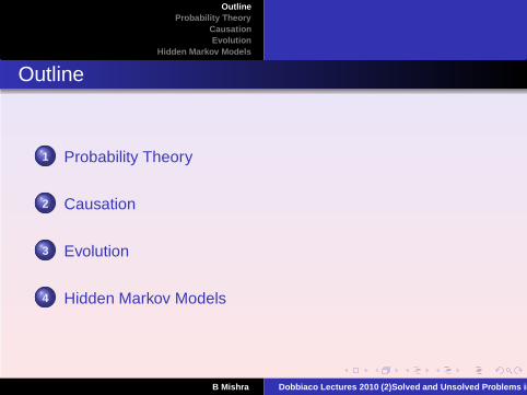
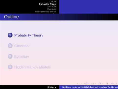
Outline
1 Probability Theory
2 Causation
3 Evolution
4 Hidden Markov Models
B Mishra Dobbiaco Lectures 2010 (2)Solved and Unsolved Problems in
OutlineProbability Theory
CausationEvolution
Hidden Markov Models
PART III : Uncertainty
B Mishra Dobbiaco Lectures 2010 (2)Solved and Unsolved Problems in

OutlineProbability Theory
CausationEvolution
Hidden Markov Models
Main theses
“...1 “...2 “A thought is a proposition with sense.3 “A proposition is a truth-function of elementary
propositions.4 “The general form of a proposition is the general form of a
truth function, which is: 〈p, ξ,¬ξ〉5 “Where (or of what) one cannot speak, one must pass
over in silence. ”
–Ludwig Wittgenstein, Tractatus Logico-Philosophicus, 1921.
B Mishra Dobbiaco Lectures 2010 (2)Solved and Unsolved Problems in
OutlineProbability Theory
CausationEvolution
Hidden Markov Models
Outline
1 Probability Theory
2 Causation
3 Evolution
4 Hidden Markov Models
B Mishra Dobbiaco Lectures 2010 (2)Solved and Unsolved Problems in

OutlineProbability Theory
CausationEvolution
Hidden Markov Models
Random Variables
A (discrete) random variable is a numerical quantity that insome experiment (involving randomness) takes a valuefrom some (discrete) set of possible values.More formally, these are measurable maps
X (ω), ω ∈ Ω,
from a basic probability space (Ω, F , P) (≡ outcomes, asigma field of subsets of Ω and probability measure P onF ).Events
...ω ∈ Ω|X (ω) = xi...same as X = xi [X assumes the value xi ].
B Mishra Dobbiaco Lectures 2010 (2)Solved and Unsolved Problems in

OutlineProbability Theory
CausationEvolution
Hidden Markov Models
Few Examples
Example 1: Rolling of two six-sided dice. Random Variablemight be the sum of the two numbers showing on the dice.The possible values of the random variable are 2, 3, . . .,12.
Example 2: Occurrence of a specific word GAATTC in agenome. Random Variable might be the number ofoccurrence of this word in a random genome of length3 × 109. The possible values of the random variable are 0,1, 2, . . ., 3 × 10⁹.
B Mishra Dobbiaco Lectures 2010 (2)Solved and Unsolved Problems in
OutlineProbability Theory
CausationEvolution
Hidden Markov Models
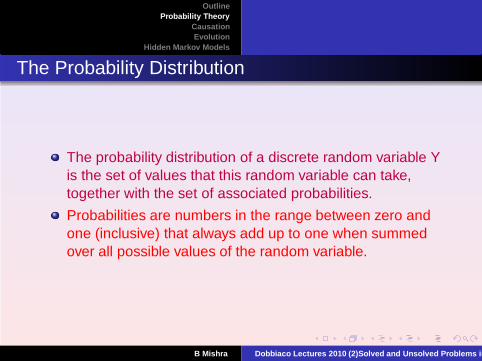
The Probability Distribution
The probability distribution of a discrete random variable Yis the set of values that this random variable can take,together with the set of associated probabilities.
Probabilities are numbers in the range between zero andone (inclusive) that always add up to one when summedover all possible values of the random variable.
B Mishra Dobbiaco Lectures 2010 (2)Solved and Unsolved Problems in
OutlineProbability Theory
CausationEvolution
Hidden Markov Models
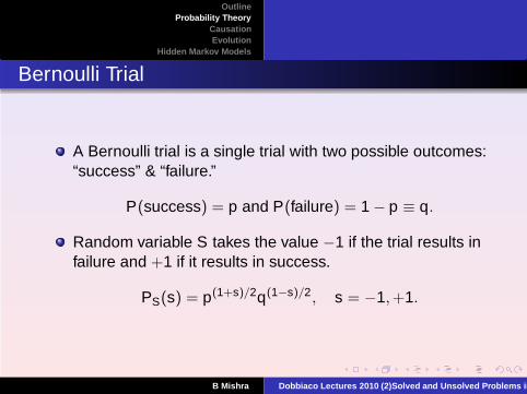
Bernoulli Trial
A Bernoulli trial is a single trial with two possible outcomes:“success” & “failure.”
P(success) = p and P(failure) = 1 − p ≡ q.
Random variable S takes the value −1 if the trial results infailure and +1 if it results in success.
PS(s) = p(1+s)/2q(1−s)/2, s = −1,+1.
B Mishra Dobbiaco Lectures 2010 (2)Solved and Unsolved Problems in
OutlineProbability Theory
CausationEvolution
Hidden Markov Models
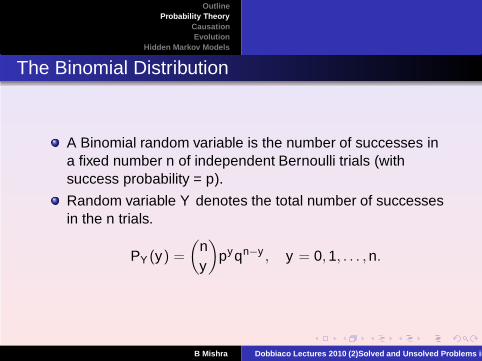
The Binomial Distribution
A Binomial random variable is the number of successes ina fixed number n of independent Bernoulli trials (withsuccess probability = p).
Random variable Y denotes the total number of successesin the n trials.
PY (y) =
(
ny
)
pyqn−y , y = 0, 1, . . . , n.
B Mishra Dobbiaco Lectures 2010 (2)Solved and Unsolved Problems in
OutlineProbability Theory
CausationEvolution
Hidden Markov Models
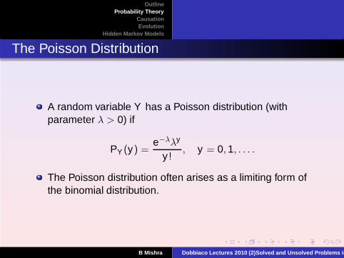
The Poisson Distribution
A random variable Y has a Poisson distribution (withparameter λ > 0) if
PY (y) =e−λλy
y!, y = 0, 1, . . . .
The Poisson distribution often arises as a limiting form ofthe binomial distribution.
B Mishra Dobbiaco Lectures 2010 (2)Solved and Unsolved Problems in
OutlineProbability Theory
CausationEvolution
Hidden Markov Models
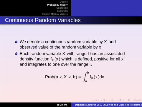
Continuous Random Variables
We denote a continuous random variable by X andobserved value of the random variable by x .
Each random variable X with range I has an associateddensity function fX (x) which is defined, positive for all xand integrates to one over the range I.
Prob(a < X < b) =
∫ b
afX (x)dx .
B Mishra Dobbiaco Lectures 2010 (2)Solved and Unsolved Problems in
OutlineProbability Theory
CausationEvolution
Hidden Markov Models
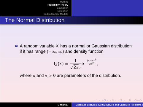
The Normal Distribution
A random variable X has a normal or Gaussian distributionif it has range (−∞,∞) and density function
fX (x) =1√2πσ
e−(x−µ)2
2σ2 ,
where µ and σ > 0 are parameters of the distribution.
B Mishra Dobbiaco Lectures 2010 (2)Solved and Unsolved Problems in

OutlineProbability Theory
CausationEvolution
Hidden Markov Models
Expectation
For a random variable Y , and any function g(Y ) of Y , theexpected value of g(Y ) is
E(g(Y )) =∑
y
g(y)PY (y),
when Y is discrete; and
E(g(Y )) =
∫
yg(y)fY (y) dy ,
when Y is continuous.Thus,
mean(Y ) = E(Y ) = µ(Y ),
variance(Y ) = E(Y 2) − E(Y )2 = σ2(Y ).
B Mishra Dobbiaco Lectures 2010 (2)Solved and Unsolved Problems in
OutlineProbability Theory
CausationEvolution
Hidden Markov Models
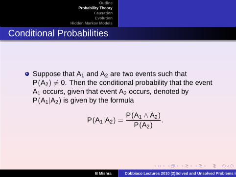
Conditional Probabilities
Suppose that A1 and A2 are two events such thatP(A2) 6= 0. Then the conditional probability that the eventA1 occurs, given that event A2 occurs, denoted byP(A1|A2) is given by the formula
P(A1|A2) =P(A1 ∧ A2)
P(A2).
B Mishra Dobbiaco Lectures 2010 (2)Solved and Unsolved Problems in
OutlineProbability Theory
CausationEvolution
Hidden Markov Models
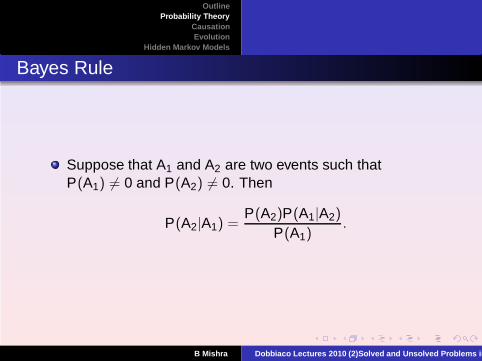
Bayes Rule
Suppose that A1 and A2 are two events such thatP(A1) 6= 0 and P(A2) 6= 0. Then
P(A2|A1) =P(A2)P(A1|A2)
P(A1).
B Mishra Dobbiaco Lectures 2010 (2)Solved and Unsolved Problems in
OutlineProbability Theory
CausationEvolution
Hidden Markov Models
Bayes Nets
Bayes Nets or Bayesian networks are graphicalrepresentation for probabilistic relationships among a setof random variables.
Given a finite set X = X1, . . . , Xn of discrete randomvariables where each variable Xi may take values from afinite set, denoted by Val(Xi).
A Bayesian network is an annotated directed acyclic graph(DAG) G that encodes a joint probability distribution over X .
B Mishra Dobbiaco Lectures 2010 (2)Solved and Unsolved Problems in
OutlineProbability Theory
CausationEvolution
Hidden Markov Models
The graph G (Bayesian Network) is defined as follows:
The nodes of the graph correspond to the randomvariables
X1, X2, . . . , Xn.
The links of the graph correspond to the direct influencefrom one variable to the other.
1 If there is a directed link from variableXi to variable Xj ,variable Xi will be a parent of variable Xj .
2 Each node is annotated with a conditional probabilitydistribution (CPD) that represents
P(Xi |Pa(Xi )),
where Pa(Xi ) denotes the parents of Xi in G.
B Mishra Dobbiaco Lectures 2010 (2)Solved and Unsolved Problems in
OutlineProbability Theory
CausationEvolution
Hidden Markov Models
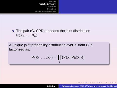
The pair (G, CPD) encodes the joint distributionP(X1, . . . , Xn).
A unique joint probability distribution over X from G isfactorized as:
P(X1, . . . , Xn) =∏
i
(P(Xi |Pa(Xi))).
B Mishra Dobbiaco Lectures 2010 (2)Solved and Unsolved Problems in
OutlineProbability Theory
CausationEvolution
Hidden Markov Models
B Mishra Dobbiaco Lectures 2010 (2)Solved and Unsolved Problems in
OutlineProbability Theory
CausationEvolution
Hidden Markov Models
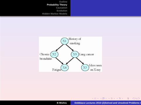
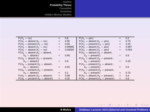
P(X1 = no) = 0.8 P(X1 = yes) = 0.2P(X2 = absent|X1 = no) = 0.95 P(X2 = absent|X1 = yes) = 0.75P(X2 = present|X1 = no) = 0.05 P(X2 = present|X1 = yes) = 0.25P(X3 = absent|X1 = no) = 0.99995 P(X3 = absent|X1 = yes) = 0.997P(X3 = absent|X1 = no) = 0.00005 P(X3 = absent|X1 = yes) = 0.003P(X4 = absent|X2 = absent, P(X4 = absent|X2 = absent,
X3 = absent) = 0.95 X3 = present) = 0.5P(X4 = absent|X2 = present, P(X4 = absent|X2 = present,
X3 = absent) = 0.9 X3 = present) = 0.25P(X4 = present|X2 = absent, P(X4 = present|X2 = absent,
X3 = absent) = 0.05 X3 = present) = 0.5P(X4 = present|X2 = present, P(X4 = present|X2 = present,
X3 = absent) = 0.1 X3 = present) = 0.75P(X5 = absent|X3 = absent) = 0.98 P(X5 = absent|X3 = present) = 0.4P(X5 = present|X3 = absent) = 0.02 P(X5 = present|X3 = present) = 0.6
B Mishra Dobbiaco Lectures 2010 (2)Solved and Unsolved Problems in
OutlineProbability Theory
CausationEvolution
Hidden Markov Models
Causal Bayesian networks
A causal Bayesian network of a domain is similar as thenormal Bayesian network — the difference is in theexplanation of the links in the Bayesian networks.
In the normal Bayesian networks, the links betweenvariables can be explained as correlation or association.In a causal Bayesian network, the links mean that theparent variables will causally influence the values of thechild variables.
B Mishra Dobbiaco Lectures 2010 (2)Solved and Unsolved Problems in
OutlineProbability Theory
CausationEvolution
Hidden Markov Models
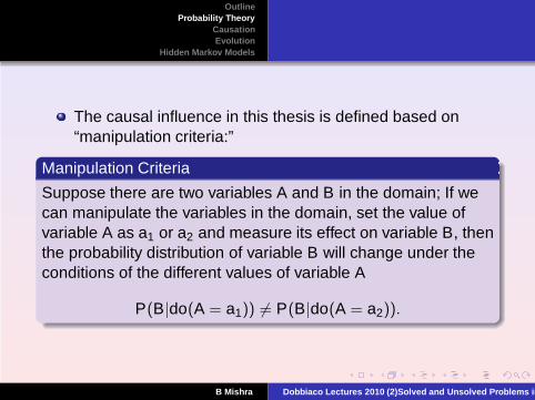
The causal influence in this thesis is defined based on“manipulation criteria:”
Manipulation Criteria
Suppose there are two variables A and B in the domain; If wecan manipulate the variables in the domain, set the value ofvariable A as a1 or a2 and measure its effect on variable B, thenthe probability distribution of variable B will change under theconditions of the different values of variable A
P(B|do(A = a1)) 6= P(B|do(A = a2)).
B Mishra Dobbiaco Lectures 2010 (2)Solved and Unsolved Problems in
OutlineProbability Theory
CausationEvolution
Hidden Markov Models
Bayesian network structure learning
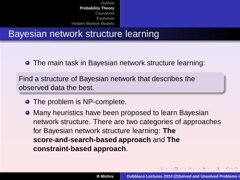
The main task in Bayesian network structure learning:
Find a structure of Bayesian network that describes theobserved data the best.
The problem is NP-complete.
Many heuristics have been proposed to learn Bayesiannetwork structure. There are two categories of approachesfor Bayesian network structure learning: Thescore-and-search-based approach and Theconstraint-based approach .
B Mishra Dobbiaco Lectures 2010 (2)Solved and Unsolved Problems in
OutlineProbability Theory
CausationEvolution
Hidden Markov Models
The score-and-search-based approach
The score-and-search-based approach:
The methods in this category start from an initial structure(generated randomly or from domain knowledge) andmove to the neighbors with the best score in the structurespace determinately or stochastically until a localmaximum of the selected criteria is reached.
The greedy learning process can re-start several timeswith different initial structures to improve the result.
B Mishra Dobbiaco Lectures 2010 (2)Solved and Unsolved Problems in
OutlineProbability Theory
CausationEvolution
Hidden Markov Models
The constraint-based approach
The constraint-based approach:
The methods under this category start to test the statisticalsignificance of the pairs of variables conditioning on othervariables to induce conditional independence.
The pairs of variables which pass some threshold aredeemed as directly connected in the Bayesian networks.
The complete Bayesian network structure is constructedfrom the induced conditional independence anddependence information.
B Mishra Dobbiaco Lectures 2010 (2)Solved and Unsolved Problems in

OutlineProbability Theory
CausationEvolution
Hidden Markov Models
How can Bayes Nets be Causal?
The causal Markov condition is a relative of Reichenbach’sthesis that “conditioning on common causes will renderjoint effects independent of other another.”One can then add the assumption of faithfulness orstability as well as to assume that all underlying systems ofcausal laws are deterministic.Similarly, using causal minimality (or sufficiency)assumption, one may try to justify the claim that “BayesianNets Are All There Is to Causality...”“Bayes nets encode information about probabilisticindependencies. Causality, if it has any connection withprobability, would seem to be related to probabilisticdependence.” (Cartwright, N.)
B Mishra Dobbiaco Lectures 2010 (2)Solved and Unsolved Problems in
OutlineProbability Theory
CausationEvolution
Hidden Markov Models
Probability Raising
“Causes produce their effects; they make them happen. So, inthe right kind of population we can expect that there will be ahigher frequency of the effect (E ) when the cause (C) ispresent than when it is absent; and conversely forpreventatives. What kind of populations are “the right kinds”?Populations in which the requisite causal process sometimesoperates unimpeded and its doing so is not correlated withother processes that mask the increase in probability, such asthe presence of a process preventing the effect or the absenceof another positive process.”
Cartwright
B Mishra Dobbiaco Lectures 2010 (2)Solved and Unsolved Problems in
OutlineProbability Theory
CausationEvolution
Hidden Markov Models
PART IV: Causation
B Mishra Dobbiaco Lectures 2010 (2)Solved and Unsolved Problems in
OutlineProbability Theory
CausationEvolution
Hidden Markov Models
Outline
1 Probability Theory
2 Causation
3 Evolution
4 Hidden Markov Models
B Mishra Dobbiaco Lectures 2010 (2)Solved and Unsolved Problems in

OutlineProbability Theory
CausationEvolution
Hidden Markov Models
B Mishra Dobbiaco Lectures 2010 (2)Solved and Unsolved Problems in
OutlineProbability Theory
CausationEvolution
Hidden Markov Models
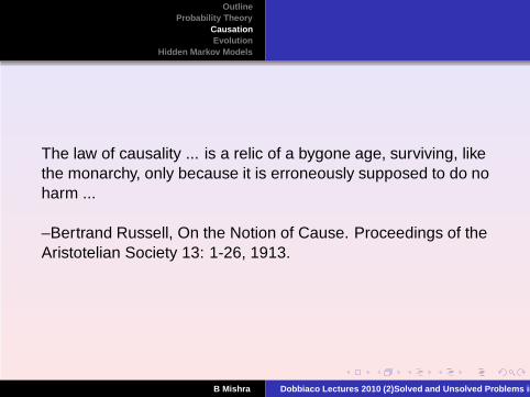
The law of causality ... is a relic of a bygone age, surviving, likethe monarchy, only because it is erroneously supposed to do noharm ...
–Bertrand Russell, On the Notion of Cause. Proceedings of theAristotelian Society 13: 1-26, 1913.
B Mishra Dobbiaco Lectures 2010 (2)Solved and Unsolved Problems in
OutlineProbability Theory
CausationEvolution
Hidden Markov Models
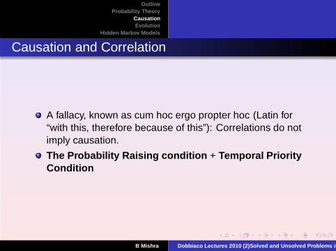
Causation and Correlation
A fallacy, known as cum hoc ergo propter hoc (Latin for“with this, therefore because of this”): Correlations do notimply causation.
The Probability Raising condition + Temporal PriorityCondition
B Mishra Dobbiaco Lectures 2010 (2)Solved and Unsolved Problems in
OutlineProbability Theory
CausationEvolution
Hidden Markov Models
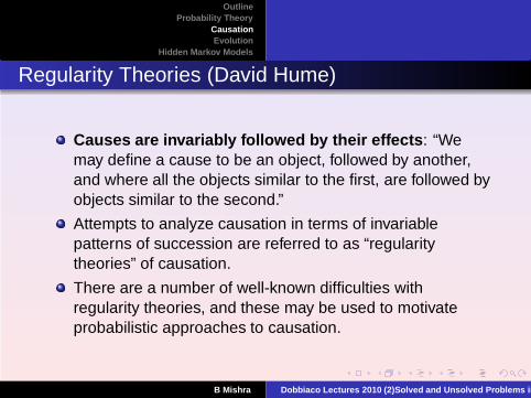
Regularity Theories (David Hume)
Causes are invariably followed by their effects : “Wemay define a cause to be an object, followed by another,and where all the objects similar to the first, are followed byobjects similar to the second.”
Attempts to analyze causation in terms of invariablepatterns of succession are referred to as “regularitytheories” of causation.
There are a number of well-known difficulties withregularity theories, and these may be used to motivateprobabilistic approaches to causation.
B Mishra Dobbiaco Lectures 2010 (2)Solved and Unsolved Problems in

OutlineProbability Theory
CausationEvolution
Hidden Markov Models
Imperfect Regularities
The first difficulty is that most causes are not invariablyfollowed by their effects.
Penetrance : The presence of a disease allele does notalways lead to a disease phenotype.
Probabilistic theories of causation : simply requires thatcauses raise the probability of their effects; an effect maystill occur in the absence of a cause or fail to occur in itspresence.
Thus smoking is a cause of lung cancer, not because allsmokers develop lung cancer, but because smokers aremore likely to develop lung cancer than non-smokers.
B Mishra Dobbiaco Lectures 2010 (2)Solved and Unsolved Problems in
OutlineProbability Theory
CausationEvolution
Hidden Markov Models
Imperfect Regularities: INUS condition
John Stuart Mill and John Mackie offer more refinedaccounts of the regularities that underwrite causalrelations.
An INUS condition : for some effect is an insufficient butnon-redundant part of an unnecessary but sufficientcondition.
Complexity : raises problems for the epistemology ofcausation.
B Mishra Dobbiaco Lectures 2010 (2)Solved and Unsolved Problems in
OutlineProbability Theory
CausationEvolution
Hidden Markov Models
INUS condition
Suppose, for example, that a lit match causes a forest fire.The lighting of the match, by itself, is not sufficient; manymatches are lit without ensuing forest fires. The lit matchis, however, a part of some constellation of conditions thatare jointly sufficient for the fire. Moreover, given that thisset of conditions occurred, rather than some other setsufficient for fire, the lighting of the match was necessary:fires do not occur in such circumstances when lit matchesare not present.
Epistasis, and gene-environment interaction.
B Mishra Dobbiaco Lectures 2010 (2)Solved and Unsolved Problems in
OutlineProbability Theory
CausationEvolution
Hidden Markov Models
Asymmetry
Causation is usually asymmetric.
If A causes B, then, typically, B will not also cause A.
This poses a problem for regularity theories, for it seemsquite plausible that if smoking is an INUS condition for lungcancer, then lung cancer will be an INUS condition forsmoking.
One way of enforcing the asymmetry of causation is tostipulate that causes precede their effects in time.
B Mishra Dobbiaco Lectures 2010 (2)Solved and Unsolved Problems in

OutlineProbability Theory
CausationEvolution
Hidden Markov Models
Spurious Regularities
Suppose that a cause is regularly followed by two effects.For instance, a particular allele A is pleiotropic... It causesa disease trait, but also transcription of another gene B. Bmay be mistakenly thought to be causing the disease.
B is also an INUS condition for disease state. But it’s not acause.
Whenever the barometric pressure drops below a certainlevel, two things happen: First, the height of the column ofmercury in a barometer drops . Shortly afterwards, a stormoccurs. Then, it may well also be the case that wheneverthe column of mercury drops, there will be a storm.
B Mishra Dobbiaco Lectures 2010 (2)Solved and Unsolved Problems in

OutlineProbability Theory
CausationEvolution
Hidden Markov Models
Causes raise the probability of their effects.
This can be expressed formally using the apparatus ofconditional probability.
Let A, B, C, . . . represent factors that potentially stand incausal relations.
Let P be a probability function... such that Pr(A)represents the empirical probability that factor A occurs oris instantiated.
Recall: P(B|A) represents the conditional probability of B,given A.
Pr(B|A) =Pr(A ∧ B)
Pr(A).
B Mishra Dobbiaco Lectures 2010 (2)Solved and Unsolved Problems in
OutlineProbability Theory
CausationEvolution
Hidden Markov Models
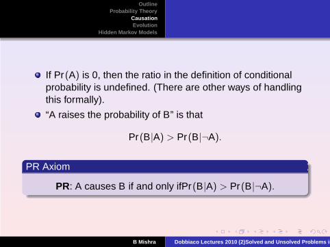
If Pr(A) is 0, then the ratio in the definition of conditionalprobability is undefined. (There are other ways of handlingthis formally).
“A raises the probability of B” is that
Pr(B|A) > Pr(B|¬A).
PR Axiom
PR: A causes B if and only ifPr(B|A) > Pr(B|¬A).
B Mishra Dobbiaco Lectures 2010 (2)Solved and Unsolved Problems in
OutlineProbability Theory
CausationEvolution
Hidden Markov Models
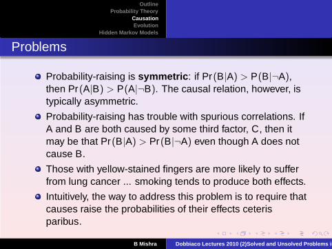
Problems
Probability-raising is symmetric : if Pr(B|A) > P(B|¬A),then Pr(A|B) > P(A|¬B). The causal relation, however, istypically asymmetric.
Probability-raising has trouble with spurious correlations. IfA and B are both caused by some third factor, C, then itmay be that Pr(B|A) > Pr(B|¬A) even though A does notcause B.
Those with yellow-stained fingers are more likely to sufferfrom lung cancer ... smoking tends to produce both effects.
Intuitively, the way to address this problem is to require thatcauses raise the probabilities of their effects ceterisparibus.
B Mishra Dobbiaco Lectures 2010 (2)Solved and Unsolved Problems in
OutlineProbability Theory
CausationEvolution
Hidden Markov Models
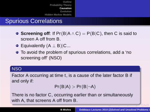
Spurious Correlations
Screening off : If Pr(B|A ∧ C) = P(B|C), then C is said toscreen A off from B.
Equivalently (A ⊥ B)|C...
To avoid the problem of spurious correlations, add a ‘noscreening off’ (NSO)
NSO
Factor A occurring at time t , is a cause of the later factor B ifand only if:
Pr(B|A) > Pr(B|¬A)
There is no factor C, occurring earlier than or simultaneouslywith A, that screens A off from B.
B Mishra Dobbiaco Lectures 2010 (2)Solved and Unsolved Problems in
OutlineProbability Theory
CausationEvolution
Hidden Markov Models
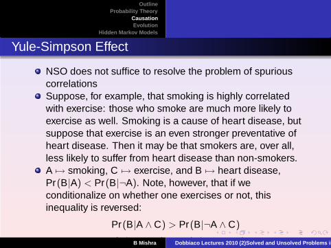
Yule-Simpson Effect
NSO does not suffice to resolve the problem of spuriouscorrelationsSuppose, for example, that smoking is highly correlatedwith exercise: those who smoke are much more likely toexercise as well. Smoking is a cause of heart disease, butsuppose that exercise is an even stronger preventative ofheart disease. Then it may be that smokers are, over all,less likely to suffer from heart disease than non-smokers.A 7→ smoking, C 7→ exercise, and B 7→ heart disease,Pr(B|A) < Pr(B|¬A). Note, however, that if weconditionalize on whether one exercises or not, thisinequality is reversed:
Pr(B|A ∧ C) > Pr(B|¬A ∧ C)
Pr(B|A ∧ ¬C) > Pr(B|¬A ∧ ¬C).B Mishra Dobbiaco Lectures 2010 (2)Solved and Unsolved Problems in
OutlineProbability Theory
CausationEvolution
Hidden Markov Models
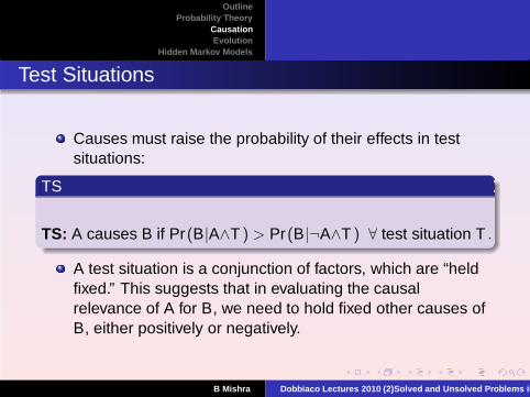
Test Situations
Causes must raise the probability of their effects in testsituations:
TS
TS: A causes B if Pr(B|A∧T ) > Pr(B|¬A∧T ) ∀ test situation T .
A test situation is a conjunction of factors, which are “heldfixed.” This suggests that in evaluating the causalrelevance of A for B, we need to hold fixed other causes ofB, either positively or negatively.
B Mishra Dobbiaco Lectures 2010 (2)Solved and Unsolved Problems in

OutlineProbability Theory
CausationEvolution
Hidden Markov Models
PART V: Evolution
B Mishra Dobbiaco Lectures 2010 (2)Solved and Unsolved Problems in

OutlineProbability Theory
CausationEvolution
Hidden Markov Models
Outline
1 Probability Theory
2 Causation
3 Evolution
4 Hidden Markov Models
B Mishra Dobbiaco Lectures 2010 (2)Solved and Unsolved Problems in

OutlineProbability Theory
CausationEvolution
Hidden Markov Models
B Mishra Dobbiaco Lectures 2010 (2)Solved and Unsolved Problems in
OutlineProbability Theory
CausationEvolution
Hidden Markov Models
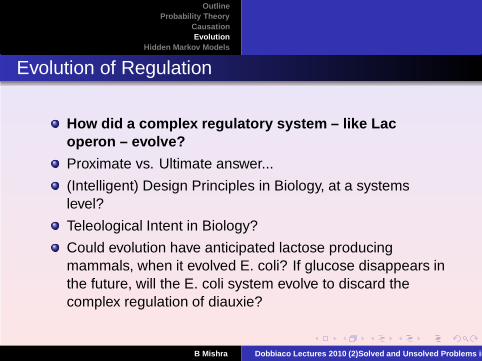
Evolution of Regulation
How did a complex regulatory system – like Lacoperon – evolve?
Proximate vs. Ultimate answer...
(Intelligent) Design Principles in Biology, at a systemslevel?
Teleological Intent in Biology?
Could evolution have anticipated lactose producingmammals, when it evolved E. coli? If glucose disappears inthe future, will the E. coli system evolve to discard thecomplex regulation of diauxie?
B Mishra Dobbiaco Lectures 2010 (2)Solved and Unsolved Problems in
OutlineProbability Theory
CausationEvolution
Hidden Markov Models
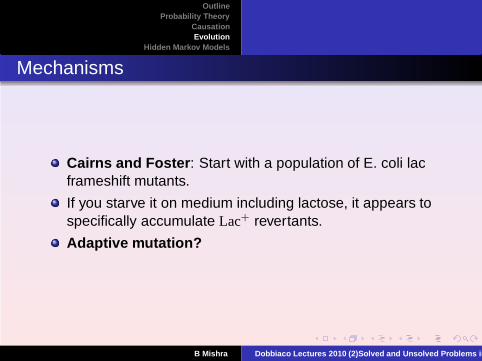
Mechanisms
Cairns and Foster : Start with a population of E. coli lacframeshift mutants.
If you starve it on medium including lactose, it appears tospecifically accumulate Lac+ revertants.
Adaptive mutation?
B Mishra Dobbiaco Lectures 2010 (2)Solved and Unsolved Problems in
OutlineProbability Theory
CausationEvolution
Hidden Markov Models
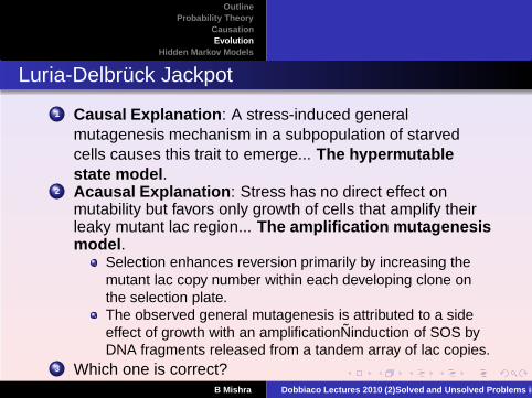
Luria-Delbruck Jackpot
1 Causal Explanation : A stress-induced generalmutagenesis mechanism in a subpopulation of starvedcells causes this trait to emerge... The hypermutablestate model .
2 Acausal Explanation : Stress has no direct effect onmutability but favors only growth of cells that amplify theirleaky mutant lac region... The amplification mutagenesismodel .
Selection enhances reversion primarily by increasing themutant lac copy number within each developing clone onthe selection plate.The observed general mutagenesis is attributed to a sideeffect of growth with an amplificationNinduction of SOS byDNA fragments released from a tandem array of lac copies.
3 Which one is correct?B Mishra Dobbiaco Lectures 2010 (2)Solved and Unsolved Problems in
OutlineProbability Theory
CausationEvolution
Hidden Markov Models
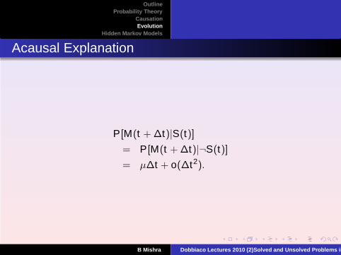
Acausal Explanation
P[M(t + ∆t)|S(t)]
= P[M(t + ∆t)|¬S(t)]
= µ∆t + o(∆t2).
B Mishra Dobbiaco Lectures 2010 (2)Solved and Unsolved Problems in
OutlineProbability Theory
CausationEvolution
Hidden Markov Models
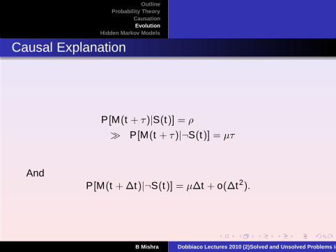
Causal Explanation
P[M(t + τ)|S(t)] = ρ
≫ P[M(t + τ)|¬S(t)] = µτ
AndP[M(t + ∆t)|¬S(t)] = µ∆t + o(∆t2).
B Mishra Dobbiaco Lectures 2010 (2)Solved and Unsolved Problems in
OutlineProbability Theory
CausationEvolution
Hidden Markov Models
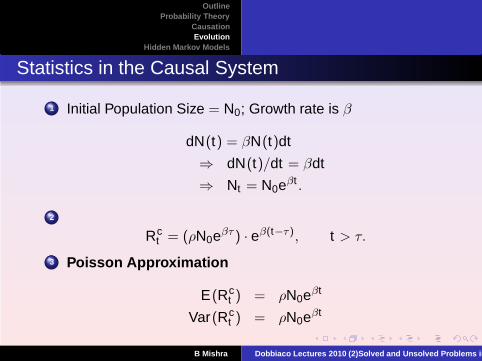
Statistics in the Causal System
1 Initial Population Size = N0; Growth rate is β
dN(t) = βN(t)dt
⇒ dN(t)/dt = βdt
⇒ Nt = N0eβt .
2
Rct = (ρN0eβτ ) · eβ(t−τ), t > τ.
3 Poisson Approximation
E(Rct ) = ρN0eβt
Var(Rct ) = ρN0eβt
B Mishra Dobbiaco Lectures 2010 (2)Solved and Unsolved Problems in
OutlineProbability Theory
CausationEvolution
Hidden Markov Models
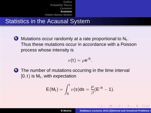
Statistics in the Acausal System
1 Mutations occur randomly at a rate proportional to Nt .Thus these mutations occur in accordance with a Poissonprocess whose intensity is
ν(t) = µeβt .
2 The number of mutations occurring in the time interval[0, t) is Mt , with expectation
E(Mt) =
∫ t
0ν(s)ds =
µ
β(Eβt − 1).
B Mishra Dobbiaco Lectures 2010 (2)Solved and Unsolved Problems in
OutlineProbability Theory
CausationEvolution
Hidden Markov Models
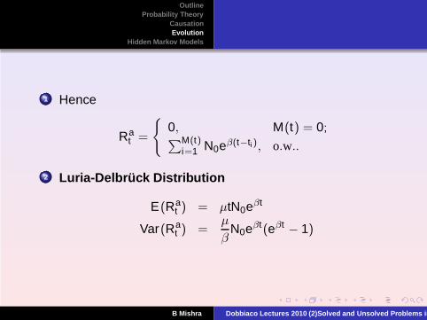
1 Hence
Rat =
0, M(t) = 0;∑M(t)
i=1 N0eβ(t−ti ), o.w..
2 Luria-Delbruck Distribution
E(Rat ) = µtN0eβt
Var(Rat ) =
µ
βN0eβt(eβt − 1)
B Mishra Dobbiaco Lectures 2010 (2)Solved and Unsolved Problems in
OutlineProbability Theory
CausationEvolution
Hidden Markov Models
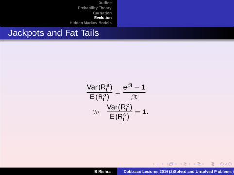
Jackpots and Fat Tails
Var(Rat )
E(Rat )
=eβt − 1
βt
≫ Var(Rct )
E(Rct )
= 1.
B Mishra Dobbiaco Lectures 2010 (2)Solved and Unsolved Problems in

OutlineProbability Theory
CausationEvolution
Hidden Markov Models
B Mishra Dobbiaco Lectures 2010 (2)Solved and Unsolved Problems in

OutlineProbability Theory
CausationEvolution
Hidden Markov Models
History
Historically, Luria-Delbruck experiment involved pure bacterialcultures (starting with a single bacterium), attacked by abacterial virus (bacteriophage). They noticed that the culturewould clear after a few hours due to destruction of the sensitivecells by the virus. However, after further incubation for a fewhours, or sometimes days, the culture would become turbidagain (due to growth of a bacterial variant which is resistant tothe action of the virus).
B Mishra Dobbiaco Lectures 2010 (2)Solved and Unsolved Problems in
OutlineProbability Theory
CausationEvolution
Hidden Markov Models
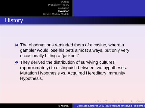
History
The observations reminded them of a casino, where agambler would lose his bets almost always, but only veryoccasionally hitting a “jackpot.”
They derived the distribution of surviving cultures(approximately) to distinguish between two hypotheses:Mutation Hypothesis vs. Acquired Hereditary ImmunityHypothesis.
B Mishra Dobbiaco Lectures 2010 (2)Solved and Unsolved Problems in

OutlineProbability Theory
CausationEvolution
Hidden Markov Models
PART VI: Time
B Mishra Dobbiaco Lectures 2010 (2)Solved and Unsolved Problems in
OutlineProbability Theory
CausationEvolution
Hidden Markov Models
Outline
1 Probability Theory
2 Causation
3 Evolution
4 Hidden Markov Models
B Mishra Dobbiaco Lectures 2010 (2)Solved and Unsolved Problems in
OutlineProbability Theory
CausationEvolution
Hidden Markov Models
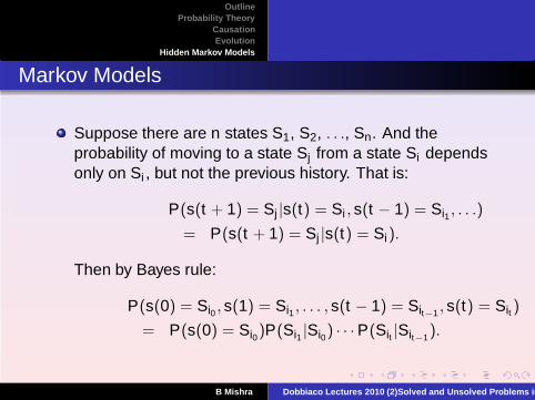
Markov Models
Suppose there are n states S1, S2, . . ., Sn. And theprobability of moving to a state Sj from a state Si dependsonly on Si , but not the previous history. That is:
P(s(t + 1) = Sj |s(t) = Si , s(t − 1) = Si1, . . .)
= P(s(t + 1) = Sj |s(t) = Si).
Then by Bayes rule:
P(s(0) = Si0 , s(1) = Si1, . . . , s(t − 1) = Sit−1 , s(t) = Sit )
= P(s(0) = Si0)P(Si1 |Si0) · · ·P(Sit |Sit−1).
B Mishra Dobbiaco Lectures 2010 (2)Solved and Unsolved Problems in
OutlineProbability Theory
CausationEvolution
Hidden Markov Models
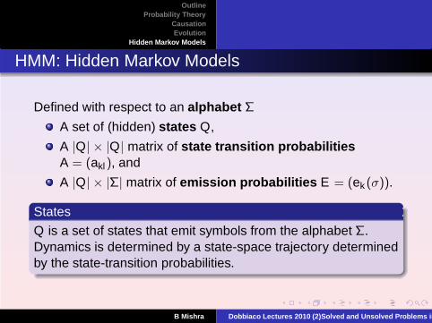
HMM: Hidden Markov Models
Defined with respect to an alphabet Σ
A set of (hidden) states Q,
A |Q| × |Q| matrix of state transition probabilitiesA = (akl), and
A |Q| × |Σ| matrix of emission probabilities E = (ek (σ)).
States
Q is a set of states that emit symbols from the alphabet Σ.Dynamics is determined by a state-space trajectory determinedby the state-transition probabilities.
B Mishra Dobbiaco Lectures 2010 (2)Solved and Unsolved Problems in
OutlineProbability Theory
CausationEvolution
Hidden Markov Models
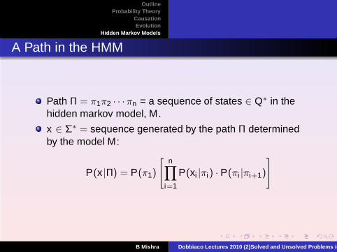
A Path in the HMM
Path Π = π1π2 · · · πn = a sequence of states ∈ Q∗ in thehidden markov model, M.
x ∈ Σ∗ = sequence generated by the path Π determinedby the model M:
P(x |Π) = P(π1)
[
n∏
i=1
P(xi |πi) · P(πi |πi+1)
]
B Mishra Dobbiaco Lectures 2010 (2)Solved and Unsolved Problems in
OutlineProbability Theory
CausationEvolution
Hidden Markov Models
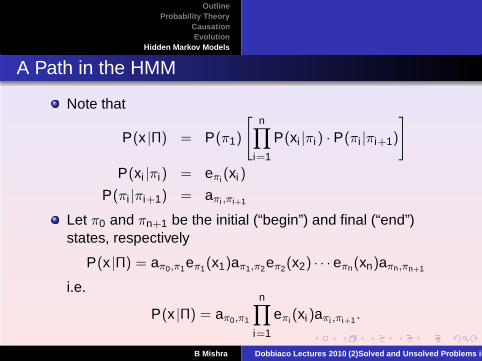
A Path in the HMM
Note that
P(x |Π) = P(π1)
[
n∏
i=1
P(xi |πi) · P(πi |πi+1)
]
P(xi |πi) = eπi (xi )
P(πi |πi+1) = aπi ,πi+1
Let π0 and πn+1 be the initial (“begin”) and final (“end”)states, respectively
P(x |Π) = aπ0,π1eπ1(x1)aπ1,π2eπ2(x2) · · · eπn(xn)aπn,πn+1
i.e.
P(x |Π) = aπ0,π1
n∏
i=1
eπi (xi)aπi ,πi+1.
B Mishra Dobbiaco Lectures 2010 (2)Solved and Unsolved Problems in
OutlineProbability Theory
CausationEvolution
Hidden Markov Models
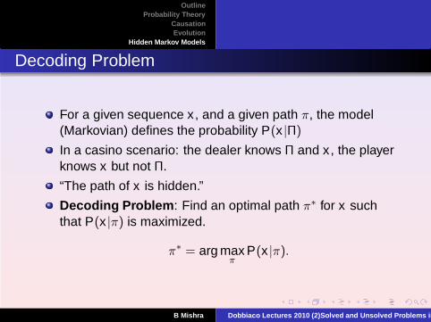
Decoding Problem
For a given sequence x , and a given path π, the model(Markovian) defines the probability P(x |Π)
In a casino scenario: the dealer knows Π and x , the playerknows x but not Π.
“The path of x is hidden.”
Decoding Problem : Find an optimal path π∗ for x suchthat P(x |π) is maximized.
π∗ = arg maxπ
P(x |π).
B Mishra Dobbiaco Lectures 2010 (2)Solved and Unsolved Problems in
OutlineProbability Theory
CausationEvolution
Hidden Markov Models
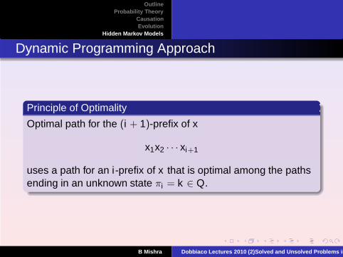
Dynamic Programming Approach
Principle of Optimality
Optimal path for the (i + 1)-prefix of x
x1x2 · · · xi+1
uses a path for an i-prefix of x that is optimal among the pathsending in an unknown state πi = k ∈ Q.
B Mishra Dobbiaco Lectures 2010 (2)Solved and Unsolved Problems in

OutlineProbability Theory
CausationEvolution
Hidden Markov Models
Dynamic Programming Approach
Recurrence: sk (i) = the probability of the most probable pathfor the i-prefix ending in state k
∀k∈Q∀1≤i≤n sk (i) = ek (xi) · maxl∈Q
sl(i − 1)alk .
B Mishra Dobbiaco Lectures 2010 (2)Solved and Unsolved Problems in
OutlineProbability Theory
CausationEvolution
Hidden Markov Models
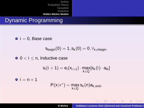
Dynamic Programming
i = 0, Base case
sbegin(0) = 1, sk (0) = 0,∀k 6=begin.
0 < i ≤ n, Inductive case
sl(i + 1) = el(xi+1) · maxk∈Q
[sk (i) · akl ]
i = n + 1P(x |π∗) = max
k∈Qsk (n)ak ,end .
B Mishra Dobbiaco Lectures 2010 (2)Solved and Unsolved Problems in

OutlineProbability Theory
CausationEvolution
Hidden Markov Models
Viterbi Algorithm
Dynamic Programing with “log-score ” function
Sl(i) = log sl(i).
Space Complexity = O(n|Q|).Time Complexity = O(n|Q|).Additive formula:
Sl(i + 1) = log el(xi+1) + maxk∈Q
[Sk (i) + log akl ].
B Mishra Dobbiaco Lectures 2010 (2)Solved and Unsolved Problems in

OutlineProbability Theory
CausationEvolution
Hidden Markov Models
[End of Lecture #2]
B Mishra Dobbiaco Lectures 2010 (2)Solved and Unsolved Problems in