doe/et/51013-137 safety and protection for large

PFC/RR-84-17 DOE/ET/51013-137

SAFETY AND PROTECTION FOR LARGE SCALESUPERCONDUCTING MAGNETS - FY1984 REPORT

by

R.J. Thome, R.D. Pillsbury, Jr., J.V. Minervini,J.M. Tarrh, H.D. Becker, W.R. Mann, U.R. Christensen,M. Pelovitz, W.G. Langton, P. Rezza, and W. Beck

November 1984

Submitted to Idaho National Engineering Laboratory

-i -

TABLE OF CONTENTS

PAGE

1.0 INTRODUCTION 1

2.0 MAGNETIC TO KINETIC ENERGY CONVERSION FOLLOWING

STRUCTURAL FAILURE 6

2.1 Foreword and Abstract 6

2.2 Introduction 7

2.3 Model Description and Results 9

2.4 Conclusions 25

2.5 References for Chapter 2 26

3.0 PROTECTION OF TOROIDAL FIELD COILS USING

MULTIPLE CIRCUITS , 27

3.1 Foreword and Abstract 27

3.2 Discharge of.Single-Circuit Systems 28

3.3 Discharge of Two-Circuit Systems 29

3.4 Discharge of Three-Circuit Systems 33

3.5 Discharge Currents and Voltages (3 Circuits) 34

3.6 Force Considerations (3 Circuits) 36

3.7 Discharge of Multiple-Circuit Systems 39

3.8 Summary and Conclusions 45

3.9 References for Chapter 3 46

4.0 HPDE MAGNET FAILURE 47

4.1 Introduction 47

4.2 Summary 47

4.3 Update of Preliminary Structural Failure Analysis 54

4.4 References -for Chapter 4 58

-ii -

TABLE OF CONTENTS CONT.

PAGE

5.0 TFCX MAGNET OPTIONS

5.1 Option Definition

5.2 Fault Conditions'

5.2.1 PF Fault Influence on PF Coils

5.2.2 PF Fault Influence on TF Coils

5.2.3 TF Fault Influence on TF Coils

5.2.4 TF Fault Influence on PF Coils

5.3 Summary

5.4 References for Chapter 5

6.0 SAFETY RELATED EXPERIMENTS

6.1 ICCS Small Football Coil

6.1.1 Measurement of Critical Current

6.1.2 Measurement of Quench Voltage and Pressure

6.1.3 Attempt to Quench to Failure of the Winding

6.1.4 Summary and Conclusions

6.2 ICCS Termination

6.2.1 Sample Termination

6.2.2 Experimental Set-Up

6.2.3 Energy Calculations

6.2.4 Test Results

6.2.5 Discussion and Summary


7.0 LABORATORY LIQUID HELIUM DEWAR FAILURE

7.1 Dewar Failure

7.2 Thermodynamic .nalysis of Pressurized Dewars -

7.3 Summary

8.0 SAFETY-RELATED ACTIVITIES

8.1 Publications

8.2 MESA Subcontract

59

59

63

64

70

72

73

73

73

74

74

79

79

89

93

94

94

95

99

102

102

108

109

109

114

119

122

122

122

0WAvWWffiWNNW

-iii-

LIST OF FIGURESPAGE

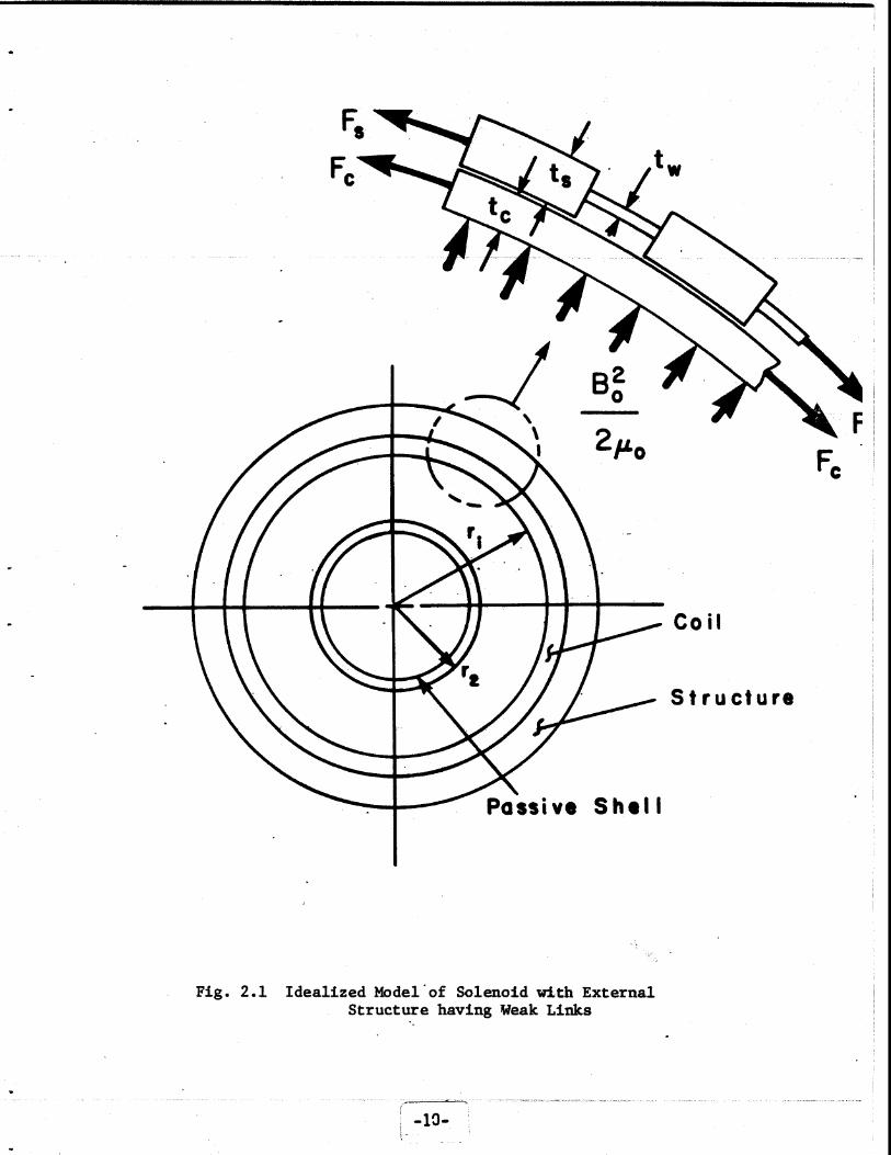
2.1 Idealized Model of Solenoid with External Structurehaving Weak Links. 10

2.2a Ideal elastic-plastic stress-strain curves for the coiland structure and typical design without "weak" links. 11

2.2b Possible design with "weak" links. 11

2.3 Element of coil and structure being accelerated radial-ly by the electromagnetic force, Fem, and restrained bythe hoop tension, Fcr, in the coil. 13

2.4 Surface in [F0 , k2, (0/T d)] space for an infinitesolenoid. 17

2.5 Normalized current vs. time for Case 2 and selectedvalues of (To/Td)- 21

2.6 Normalized radial displacement vs. time for Case 2 andselected values of (To/Td)- 22

2.7 Normalized kinetic energy vs. time for Case 2. 23

3.1 Normalized maximum discharge voltage as functions ofthe coupling coefficient for a system having twocircuits. 32

3.2 Normalized maximum discharge voltages as functions ofthe coupling coefficient for a system having three cir-cuits, discharged under conditions of equal finaltenperatures. 37

3.3 Normalized discharged time constants as functions ofthe coupling coefficient for a system having three cir-cuits which are discharged sequentially under condi-tions for equal final temperatures. 38

3.4 Approximate normalized out-of-plane forces on the in-board leg as a function of the normalized major radiusfor various numbers of coils in a system having threecircuits. 40

3.5 Approximate normalized out-of-plane forces on the out-board leg as functions of the normalized major radiusfor various numbers of coils in a system having threecircuits. 41

3.6 Sketch of a typical TF coil for TFCX, which includes 16TF coils, each having a thickness of 0.541 m. 43

4.1 Overall view of the assembled magnet system. 49

-iv-

LIST OF FIGURES CONT.PAGE

4.2 HPDE Saddle Magnet Coils: 6.8 T Design Lorentz Forces. 50

4.3 Aluminum Force Containment Structure (FCS) 51

4.4 Exaggerated depiction of LTM-related deflections at themagnet midplane. 52

4.5 Collar corner behavior. 53

5.1 Comparison of TF Coil Characteristics 60

5.2 EM loads per unit length on PF coils at start of burnwith plasma. 62

5.3 Typical case of symmetric PF coil fault and PF circuitcurrent changes. 65

5.4 PF coil designations for fault study responses. 66

5.5 Illustration of PF interactions with a TF coil. 71

6.1 Cross section of conductor used in small football test. 76

6.2 Outline of mandrel for small football test. 77

6.3 Photo of small football coil wound on mandrel withside support plates in place. 78

6.4 Schematic of helium flow path for small football coiltest. 80

6.5 Schematic of experimental set-up. 81

6.6 Critical current results of small football coil. 82

6.7 Coil current, voltage and pressure traces as a func-tion of time during Event A. 85

6.8 Coil current, voltage and pressure traces as a func-tion of time during Event B. 87

6.9 Coil current, voltage and pressure traces as a func-tion of time during Event C. 88

6.10 Coil current, voltage and pressure traces as a func-tion of time during Event D. 90

6.11 Trace of voltage drop across the vapor-cooled cur-rent leads during Event D. 91

6.12 Termination Assembly. 96

-v-

LIST OF FIGURES CONT. PAGE

6.13 Termination test section with copper current transferblock and voltage taps attached. 97

6.14 Schematic of experimental set-up for ICCS terminationtest. 98

6.15 Adiabatic heating of copper. 101

6.16 Oscilloscope traces of conductor current and voltageversus time. 103

6.1.7 Conductor resistance versus time. 104

6.18 Power dissipated versus time. 105

6.19 Termination test section after burnout showing cableburned completely through. 106

7.1 Simplified cross section of liquid helium dewar. 110

7.2 Two views of dewar after explosion. 112

7.3 View of dewar and laboratory damage after explosion. 113

7.4 Temperature and pressure in a container filled withenough liquid helium to reach a given vapor volumefraction, then sealed at 15 psia and subjected to agiven total heat input per unit mass. 116

7.5 Model of helium flow through burst disc for a givenheat input rate. 118

7.6 Heat removed per unit burst disc area as a functionof pressure rise in the container and stagnation tem-perature of the flow. 120

-vi-

LIST OF TABLES

PAGE

2.1 Hypothetical Solenoid Characteristics. 19

3.1 Characteristics of Two-Circuit Systems. 33

3.2 Characteristics of Three-Circuit Systems. 35

3.3 Characteristics of TFCX. 44

5.1 Ratio of number of "Large" Excursions to Number ofFaults for PF Interactions with PF Coils. 67

5.2 Range of Fault Factors for PF Interactions with PFCoils. 68

6.1 Small Football Coil Conductor Parameters. 75

ACKNOWLEDGMENTS

The authors would like to express their appreciation to A.M. Dawson

for editing and. B.A. Keesler and D. Marble for report preparation.

1.0 INTRODUCTION

The Fusion Program is moving rapidly into design and construction of

systems using magnets with stored energies in the range of hundreds of

megajoules to gigajoules. For example, the toroidal field coil system

alone for TFCX would store about 4 GJ and the mirror system MFTF-B would

store about 1.6 GJ. Safety and protection analyses of the magnet subsys-

tems become progressively more important as the size and complexity of the

installations increase. MIT has been carrying out a program for INEL ori-

ented toward safety and protection in large scale superconducting magnet

systems. The program involves collection and analysis of information on

actual magnet failures, analyses of general problems associated with safe-

ty and protection, and performance of safety oriented experiments. This

report summarizes work performed in FY84.

In last year's report, we summarized effort in three areas that were

continued th.is year. These are covered in Sections 2.0, 3.0 and 4.0 which

present the new results, but which are self-contained for the sake of con-

venience.

Section 2.0 considers the parameters which influence the conversion

of the stored magnetic energy to kinetic energy of ruptured components in

the event of a major structural failure. Last year's specific results are

summarized and were extended this year to the more general result which

defines a surface in parameter space that separates systems into groups

that either allow or prevent a substantial fraction of the initial stored

energy to be converted to kinetic energy.* The important parameters are

*R.J. Thome, R.D. Pillsbury, Jr., W.G. Langton and W.R. Mann, "Magneticto Kinetic Energy Conversion Following Structural Failure," presented atApplied Superconductivity Conference, San Diego, CA, September 1984.

-1-

shown to be the relative winding ultimate strength, the coupling coeffi-

cient to a secondary circuit, and the ratio of the time scale for compon-

ent acceleration to the time scale for ohmic dissipation. The conclusions

are: (a) a protective circuit reaction involving resistive dissipation

following a major structural failure is unlikely to be effective on a fast

enough time scale in high current density windings; (b) windings with

low enough current densities can absorb the total load following struc-

tural failure, thus limiting the kinetic energy conversion process, al-

though this might involve substantial yielding and deformation of the

winding; and (c) protective circuits involving inductive energy transfer

can respond fast enough to limit the kinetic energy conversion process in

high or low current density configurations and are effective provided they

are well coupled to the primary circuit.

Section 3.0 extends last year's effort in study -of the advantages of

protecting toroidal field coil systems with multiple circuits. The more

general results* are presented in five figures and two tables which relate

the maximum discharge voltages in two and three circuit systems to the

coupling coefficient and relate the out-of-plane forces in a three circuit

system to the number of coils in the system and the normalized major ra-

dius. A specific example based on an early TFCX TF coil design is given.

The primary disadvantages of multiple circuits are the increased circuit

complexity and potential for out-of-plane forces. These are offset by the

substantial reduction in maximum discharge voltages, as well as other de-

sign options which become available when multiple circuits are used.

*R.J. Thome, J.M. Tarrh, R.D. Pillsbury, Jr., W.R. Mann and W.G. Langton,"Protection of Toroidal Field Coils Using Multiple Circuits," presented atEngineering Problems of Fusion Research, Philadelphia, PA, December 1983,IEEE Cat. No. 83CH1916-6 NPS, pp. 2059-2063.

-2-

Section 4.0 completes our studies relative to the structural failure

of a large magnetohydrodynamic (MHD) magnet in December 1982. The event

led to brittle-fracture failures in most of the structural components,

significant displacements (on the order of a meter) of some of the magnet

iron frame components, and similar deformation of the winding with some

conductor fracture. Our FY1983 report contains a detailed description of

the magnet system, a summary of the failure, and the results of a prelim-

inary structural failure analysis. This section contains a brief intro-

ductory summary of the magnet system and cause of failure, and an update

of the previous analysis to document work performed during FY1984.

A preliminary study of fault load conditions was carried out for

three of the options under consideration for TFCX. The specific char-

acteristics of the cases are defined in Section 5.0 and the alteration in

electromagnetic loads under specific TF and PF fault conditions are

compared. In many instances, loads are nontrivial, but are believed to

be manageable through proper structural and protection circuit design.

They indicate a need for ultimate specification of a list of credible

faults and their consideration in the design process. Sixteen fault con-

ditions were considered relative to usual operating conditions at the

start of burn. Other points in the start-up, burn and shut-down scenario

require analysis at a later stage in design and could yield fault factors

which meet or exceed the ranges given. The number of conditions which re-

quire consideration is an order of magnitude larger. The process is

straightforward, but tedious, and requires development of codes which can

allow a large number of cases to be treated without the interactions now

required for transcription and reduction of inputs and outputs.

-3-

Relatively small scale, safety-related experiments which have been

conducted during FY1984 are summarized in Section 6.0. These involved

tests on a small "football" shaped coil wound with a Nb 3Sn internally

cooled cabled superconductor (ICCS) and tests on a sample ICCS termina-

tion. The football-shaped coil was tested to measure current, voltage,

and pressure during a quench. During the tests the coil pressure was

calculated to be 59 psia which is within a factor of 2 of the extrapo-

lated maximum measured pressure of 34 psia. This indicates that a simple

expression for maximum pressure rise during a quench provides a conserva-

tive estimate for cable-in-conduit conductors. In another test, an ICCS

termination was fabricated and tested to investigate failure behavior

due to conductor overheating. The conductor was energized to 1000 am-

peres at room temperature; it burned through in 3.5 seconds. The conduc-

tor failed at the weakest point in the test section., The adiabatic heat-,

ing curve for copper was used to estimate the time to burnout and was

found to be conservative within a factor of 2 of the actual value.

In March 1984, the FBNML experienced a major liquid helium dewar fail-

ure in a small storage dewar in one of the laboratory rooms. Section 7.0

describes the dewar failure, its probable causes, and some safety precau-

tions that should always be taken. In addition, a basic thermodynamic an-

alysis of dewar pressurization is given that provides insight into safe de-

war operation.

Safety and protection analyses of subsystems become progressively

more important as the stored energy increases with each successive genera-

tion of superconducting magnets. If the multigigajoule magnets for future

-4-

fusion facilities are to be operated reliably and safely, a thorough under-

standing of this area is essential. This program is contributing to this

understanding through the insight gained in fundamental analyses and small

scale testing.

-5-

2.0 MAGNETIC TO KINETIC ENERGY CONVERSION FOLLOWING STRUCTURAL FAILURE

R..J. Thome, R.D. Pillsbury, Jr., W.G. Langton and W.R. Mann

2.1 Foreword and Abstract

This effort was begun in FY83 and extended in FY84 to produce the

more general formulation represented by Fig. 2.4. Results were prepared

for presentation at the 1984 Applied Superconductivity Conference, San

Diego and will appear in the Proceedings to be published by the IEEE. The

contents of the paper are given in this chapter which is a self-contained

summary of the FY83 and FY84 work.

A magnet failure which is potentially catastrophic in the sense that

structural components fracture and the winding suffers extensive plastic

deformation can be "safe" under special conditions. It may be desirable

to limit operating current densities to levels at. which the winding could

act to limit magnetic to kinetic energy conversion. A solenoid model was

used to analyze and determine the important governing parameters in the

failure and discharge process. The conclusions are: (a) a protective cir-

cuit reaction involving resistive dissipation following a major structural

failure is unlikely to be effective on a fast enough time scale in high

current density windings; (b) windings with low enough current densities

can absorb the total load following structural failure, thus limiting the

kinetic energy conversion process, although this might involve substan-

tial yielding and deformation of the winding; (c) protective circuits

involving inductive energy transfer can respond fast enough to limit the

kinetic energy conversion process in high or low current density config-

urations and are effective provided they are well coupled to the primary

circuit.

-6-

2.2 Introduction

In late 1982, a massive structural failure occurred in a large MHD

type magnet.1,2 The magnet utilized about 8.4 x 104 kg of copper conduc-

tor, 5.4 x 104 kg of aluminum structure, and 5 x 105 kg of steel in a

flux return frame. The failure occurred at a field level of 4.1 T and

led to brittle fractures in most of the structural components, significant

displacements of some portions of the iron frame, and substantial deform-

ation of the winding with some conductor fracture. The magnet failure

was catastrophic in the sense that most structural components were broken

and the winding suffered extensive plastic deformation. However, oper-

ating procedures prevented possible injury to personnel and the rugged

nature of the winding limited deformations to large but safe values, and

restrained conversion of magnetic to kinetic energy of failed components.

Instrumentation data implied that component fracture and displace-

ments occurred on a time scale of a few to 10's of milliseconds (which

implies fractured component velocities of the order of 50 mph). Data

show that status monitoring equipment initiated an automatic shutdown on

a 100 ms time scale and that several manual shutdown signals were initi-

ated within - 2 seconds. A fraction of the magnetic field decreased

suddenly due to the flux redistribution associated with winding expan-

sion, then remained on for 10's of seconds as the remaining energy was

dissipated sa-fely. Thi.s "remaining energy" has been estimated at - 70%

of the initial magnetic field energy and was unavailable for conversion to

kinetic cnergy primarily because the winding had sufficient cross section

to carry the load in its deformed state without rupture while the energy

dissipated resistively.

-7-

This experience is relevant to superconducting magnet design since

we continually attempt to increase the winding pack current density be-

cause of cost, availability of new materials, and restrictions on space

imposed by other subsystems. As we strive for high current density, we

should recognize that we may be moving into a regime where the winding

can no longer restrain the magnetic to kinetic energy conversion process

in the event of a major structural failure. This implies the possible

need for different structural design criteria for high current density

designs where the winding would not be able to assume a deformed, but

"fail -safe" confi gurati on.

The following section presents an analysis of a simple model to

illustrate the time scales and important parameters in the event of a

major structural failure. A general plot i-s given which illustrates the

relevance of winding cross section (current density), the ineffectiveness

of resistive dissipation on a short time scale and the effectiveness of

an inductively coupled secondary provided the coupling coefficient is

sufficiently high. The analysis is applied to two hypothetical supercon-

ducting solenoids to illustrate the dependence on current density.

-8-

2.3 Model Description and Results

Figure 2.1 shows a long thin solenoid consisting of a coil, an exter-

nal structure, and an internal passive shell which might be a winding

bobbin or a secondary winding. The coil produces a magnetic field B0

within the bore and has a radial build tc and length to. The magnetic2

field produces an outward radial pressure, Bo/(2 "o) which is reacted

by hoop tension Fc in the coil and FS in the structure. The structure is

assumed to be composed of a series of alternating strong and weak links

where the latter are the conceptual equivalent of fasteners, welds or

other stress concentrators in the structural material.

The stress and strain in the materials are determined by a force

balance, geometric compatibility, and the constitutive relations for the

materials. Assume the ideal elastic/plastic stress-strain curves given

in Fig. 2.2a which show the yield strengths for the- structure and coil

materials (awy and acy, respectively) and the ultimate strain capability

of the coil corresponding to winding rupture (Cu). Figure 2.2a also illu-

strates a typical design point without weak links (tw = ts) where the coil

and structure have the same strain and operate at some fraction of their

respective yield strengths. Figure 2.2b, on the other hand, shows a possi-

ble condition when links are present which are weak enough (i.e., tw is

small enough in the model) so that the links are loaded beyond yield and

stretch plastically.

Assume t.at the coil is repeatedly charged and discharged and that,

after a number of cycles, the weak links fail with the materials in the

charged state, c, s and w, at time = t = 0. At t = 0 the entire elec-

tromagnetic load transfers to the coil and subsequent events depend

-9-

F

F t - t

t C

BZ~0

Coil

StrP

Passive Shell

cture

Fig. 2.1 Idealized Model'of Solenoid with ExternalStructure having Weak Links

-13-

S OWy Structure

asSCoil

Fig. 2.2a Ideal elastic-plastic stress-strain curves for thecoil and structure and typical design without "weak" links

T(7- St ru ct ur.

sW

OC y Coil

Fig. 2.2b Possible design with "weak"' links

-11-

strongly on whether the load is of sufficient magnitude and maintained

for a long enough time interval to strain the coil material into the

plastic range and up to its ultimate strain, eu, at which point the coil

material also ruptures. If the latter occurs, the remaining magnetic

energy is available to accelerate the components outward.

For simplicity, the weak links will be assumed to break simultane-

ously and uniformly around the periphery. Figure 2.3 then illustrates the

force balance in which the electromagnetic load is accelerating the mass

outwards, but is restrained by the hoop tension in the coil. The force

balance may be written as follows:

(82/2/po) r to de + f(12) - 2Fcr sin (de/2)

= (Mt do/2/w)(d 2r/dt 2 ) (2.1)

where: Mt total mass of coil and structure, f1 2) = force due to current

in passive secondary winding.

As the coil expands radially, its cross section necks down such that

tcr = tcri/r where: tc = initial coil thickness when at radius, ri, and

tcr = coil thickness when expanded to a radius r.

The restraining force, Fcr, provided by the. coil depends on whether

the coil material is in the elastic range, plastic range or beyond its

ultimate strain. Following the nomenclature in Fig. 2.2b, this becomes

Ec (r/rj-1) tc to, if (r/ri-1) < acy/Ec

Fcr = acy tc to 9 if (r/rj-1) > acy/Ec (2.2)

0 , if (r/ri-1) > eu

-12-

B2 rIod9 +f (12 ) = Fem2 Lo

FCoil Mass

d8 +Structural Mass

22Mt d8 d?-r dO2r dt2 2

8 Fc rFr

Fig. 2.3 Element of coil and structure being accelerated radially bythe electromagnetic force, Fem,and restrained by the hooptension, F cr, in the coil.

-13-

The electromagnetic force is determined by B which is dependent on

the current in the coil, the current in the secondary, and the circuit

characteristics. Assume the circuit to be the coil with an initial in-

ductance, Lo, in series with a resistor R(t) which can be later specified

to characterize a superconducting coil with a discharge resistor or a

conventional resistive coil. The circuit equations are given by

d(LI)/dt + IR(t) + d(MI2 )/dt = 0 (2.3)

where: M = mutual inductance between the original winding and the second

circuit or electrically conducting body; 12 = current in second circuit;

L2 (d12/dt) + d(MI)/dt + 12R2 = 0 (2.4)

where: L2 = self inductance of second circuit; R2 = resistance of the

second circuit.

If the winding and passive shell are infinitely long, then: (a) 12

in the shell will create no field at the coil, hence f(12) = 0 in (2.1);

and (b) M is not a function of r or t. Furthermore, if the time constant

for the secondary (L2 /R2 ) is assumed to be long compared to the charac-

teristic time. for the transient, To, then the above equations can be com-

bined and cast in the following dimensionless form.

(n - k2 ) d + 21n n - + (ro/Td)InTl2 0 (2.5)dT dT

n n2 FPd2 2n In - Fay = d----

d&2 (2.6)

- -------

where: n = r/ri

k2 = M2/(L0 L2) = coupling coefficient

In = I/Io

Io = initial current

T. = t/To

Mtrj

= 2 w r B02/(2 po)

Lo = initial inductance of coil

Ro = characteristic resistance =LO/To

Td = LO/R

Ri = initial coil resistance

Ec/ocy (n -1) if (n -1)< ocy/Ec

Y =1 if (n -1)> acy/Ec

0 if (n-1)> eu

0cy tc toFo = BO 2

ri to

The independent variable in Eqs. (2.5) and (2.6) is T, the normal-

ized time; the dependent variables are n, the normalized radius, and Ins

the normalized current; Td is the characteristic discharge time for the

coil alone; Y is a function of n which determines if the restraining

force supplied by the coil is in the elastic or plastic range or if the

coil has been strained beyond rupture. Fo is a parameter determined by

the characteristics of the coil structural system. It is a measure of

the maximum load carrying capabilities of the coil at yield relative to

the initial magnetic load. The characteristic time, To, is a measure

-15-

of the time required to accelerate the entire mass of the system a dis-

tance ri under the unrestrained action of the total magnetic force ini-

tially available.

The governing equations are nonlinear, but can be written in finite

difference form and integrated forward in time to determine In and n.

The initial conditions (T = 0) are that In = 1, n = 1 + ec and dn/dt = 0.

Note that the character of the system response will be critically depen-

dent on: (a) the magnitude of F0 , because F0 > 1 implies that the winding

has sufficient strength without structure to carry the entire initial

load without yield; (b) k2 , because this determines the amount of the ini-

tial stored energy which'is trapped by the secondary and is unavailable

for conversion to kinetic energy even if rupture occurs; and (c) (ro/Td)

because this governs the rate of energy dissipation in the coil circuit

and thus reduces the amount available for further winding deformation

and/or conversion to kinetic energy.

Once acy/Ec and Cu are selected we would like to choose F0 , k2 and

(To/Td) such that the coil would not strain beyond Cu even if the struc-

ture failed. The surface separating final conditions with strain < eu

from those with strain > eu for the thin solenoid model is given in Fig.

2.4 which is based on eu = 0.2 and Eckacy = 900 (the latter is considered

typical for a winding composite). In this figure, a system with a point,

Fo, k2, (To/Td), which lies inside the surface will have its winding

strained beyond eu and ruptured following structural failure whereas a

system whose point lies outside the surface will not exceed eu. In the

latter case, the winding may or may not deform plastically depending on the

location of the point, but the design point is "safe" in that the magnetic

-16-

I .0E =0.2

E "y,= 900

LL? 0.8 Ec = 5x 10 4

0

0.6 0.01

~0.

0.3C

-0.4 -0.5

0.2-ail:

00;02

0 0.2 0.4 0.6 0.8 1.0

Coupling Coefficient, k

Fig. .2.4 Surface in [F , k2 , (T /Td)] space for an infinite solenoid;windings will not rupiure for design points outside thesurface even if the structure fails.

-17-

energy will not be converted to kinetic energy of fractured winding com-

ponents. If the secondary is present (k2*0) then it oust, of course, be

capable of carrying the load associated with the magnetic energy it traps.

Figure 2.4 shows that an F0 less than 1 is still acceptable even if k2

and (To/Td) = 0 because of the energy absorption capability of the winding

as it deforms. This value will depend on Ec/lcy and eu. It also shows

that (To/Td) must be greater than about 0.1 in order for resistive dis-

sipation to have a significant impact. Since To may be expected to be

of the order of 10 ms, this implies a required discharge time constant of

the order of 100 ms with zero reaction delay. In a large system, a dis-

charge at that rate would probably correspond to an unacceptably high

voltage. As a result we conclude that resistive dissipation cannot be

considered a primary means for justifying a design at reduced Fo. Induc-

tive coupling to a secondary, on the other hand, reacts virtually instan-

taneously and is effective provided the coupling coefficient is suffici-

ently high.

The difference in system behavior can be illustrated with the two

hypothetical cases in Table 2.1 which have the same initial field and bore

size but different winding current densities. Case 1 is for a moderate

to high current density and Case 2 is for a high current density. They

lead to substantially different values for tc. The structural build, ts,

is based on a stress as = 2.76 x 108 N/m2 (4 x 104 psi). The total mass is

that of the structure based on a steel density of 7.8 x 103 kg/m 3 and the

winding based on 8.9 x 10 3 kg/m 3 with a packing factor of 0.7 applied to

the latter. If an operating current level of 2 x 104 A is chosen then the

inductance and stored energy per unit length can be shown to be 0.625 H/m

-18-

TABLE 2.1

HYPOTHETICAL SOLENOID CHARACTERISTICS

CASE

Magnetic Field, [T]

Bore Radius, [m]

Windin Cu Erent Density,[109A/m ]I

Winding Radial Build, tc [m]

Structural Build, ts [m]

Total Mass Per Unit Length,M/t 0 , [kg/m]

Operate Current, [kA]

Inductance Per Unit Length,Lo/10, [H/m]

Stored Energy Per Unit Length,E/to, [J/m)

Wingling Modulus/Yield Stress,Eclacy

Winding Strain, Cc

Characteristic Time, T0 [s]

Relative Winding Strength, F0

Winding Ultimate Strain, eu

1

10

1.0

1.860.482

0.182

3.39 x 104

20

0.625

1.25 -x 108

900

5 x 10-4

1.17 x 10-2

1.0

0.2

2

10

1.0

3.30.241

0.168

2.51 x 104

20

0.625

1.25 x 108

900

5 x 10-4

9.28 x 10-3

0.562

0.2

1 9-

and 125 MJ/m, respectively. The ratio of winding modulus to yield strength

was assumed to be 900 and the ultimate winding strain at fracture was as-

sumed to be 20%. In both cases the initial strain in the winding at the

operating current level was taken as 5 x, 10- 4 . The characteristic time,

To, is about 10 ms for each case. This is representative of the time re-

quired for the magnetic energy to accelerate the system mass and is quite

rapid. The yield stress for the winding was assumed to be acy = 0.7

(2 x 104) = 1.4 x 104 psi. This value, together with some of the charac-

teristics found earlier, allow F0 to be found. Since it is unity for

Case 1 and substantially less than one for Case 2, we expject different

responses in the event of a structural failure. Case 1 may be shown to

deform plastically, but, because F0 = 1, the winding will not rupture

even if k2 = 0 and (T0/Td) = 0 and it is, therefore, "safe."

.Figures 2.5, 2.6 and 2.7 show the response for Case 2 following a

structural failure at t = 0. The abscissa in each figure is time normal-

ized to To. Figure 2.5 shows the current in the coil normalized to the

initial current and the transient which results for four different values

of (To/Td). The case of (ro/ d) = 0 corresponds a zero resistance

situation and increasing (To/Td) implies circuitry with successively

larger resistances (quench or dump resistors). Note that the transient

is well underway in only two times the characteristic time, To. The

normalized radial displacement is shown in Fig. 2.6 over the same time

period and illustrates substantially different reactions depending on the

value of (To/Td). Higher values of (To/Td) generate a condition where

sufficient energy is dissipated rapidly enough in the resistance to limit

the deformation. However, low values result in a deformation which is

-20-

1.0

0

'-

I

0.4I

0.8I I

1.2 1 .6

Normalized Time,,t/T

Fig. 2.5 Normalized current vs time for Case 2 and selectedvalues of (T / d).

-21-

0.5 0.3 0.1 0 To/Td

Ra= (To /Td)n 2

= 0.562

0.8

0.6

0.4

0.2

Case 2:

00 2.0

I I

-

c-1.6-

Case 2: F =0.562o 1.4-00

n2R (To/Td)

- (r/d)= o

0.1

0.3

0.5Z

04 0.8 1.2 1.6 2

Normalized Time t/)

. . ... .. ........ . i,.. . . 6 N o r m a l i z e d r a d i a l d i s p l a c m e n t v s t m e f o r C a e 2and selected value OfT /Td-20-

c 0.5% I I

0.4-w

wCase 2. F= 0.562

03

&- R CM

w

~0.2

0.1-

(T/Td) a 0

E 0.10

0 0.4 0.6 1.2 1.6. 2Normalized Time,ft /T

Fig. 2.7 Normalized kinetic energy vs time for Case 2.

-23-

not limited. The critical condition occurs when the ultimate winding

strain, eu,. is exceeded. In these examples, e = 0.2; therefore, if con-

ditions are such that n - 1 + eu - 1.2 we would expect the winding to rup-

ture and no restraint on conversion of the remaining magnetic energy to

kinetic. This is shown in Fig. 2.7 which is a plot of the instantaneous

kinetic energy per unit length normalized to the magnetic energy per unit

length initially stored at t = 0. For high enough (ro/Td) the kinetic

energy starts at zero, rises to a maximum and decreases to zero. How-

ever, if the energy is not dissipated fast enough, that is, if (To/Td)

is low enough, then the. coil ruptures and the unrestrained magnetic to

kinetic energy conversion occurs. Note that the sudden change in slope

in Fig. 2.7 occurs at the time when the radial displacement in Fig. 2.6

passes through n 1.2 where the ultimate winding strain is exceeded.

Case 2 illustrates that the unrestrained conversion of magnetic to

kinetic energy can be averted even if F0 < 1, provided the usual discharge

time constant is of the same order as To. In many cases, however, this

would require unrealistically high voltages and unrealistically fast

circuit response times since To is likely to be small. As a result we

suspect that in many cases, a response involving resistive dissipation

alone is not feasible. The inductive initiation of current in a secon-

dary, however, can occur virtually instantaneously provided L2/R2 >> TO-

If the coupling coefficient to the secondary were high enough, then the

winding would not strain beyond eu even if (To/Td) = 0 and F0 < = 1. As

an example, Fig. 2.4 shows that winding rupture for Case 2 and (To/Td)

= 0 will not occur provided k2 > 0.54. The secondary must of course be

able to carry the load associated with the magnetic energy it traps.

-24-

2.4 Conclusions

Although the geometry in the previous section is simple it allows

the important parameters to become apparent and the following conclusions

to be drawn: (a) a protective circuit reaction involving dissipation in

resistive elements following a major structural failure is unlikely to be

effective on a fast enough time scale to limit the magnetic to kinetic

energy conversion process in magnets using high current density windings;

(b) protective circuits involving inductive energy transfer can respond

fast enough to limit the kinetic energy conversion process in high or low

current density configurations and can be effective if the coupling coef-

ficient is high enough; (c) windings with low enough current densities

can absorb the total load following structural failure, thus limiting the

kinetic energy conversion process, although this might involve substan-

tial yielding and deformation of the winding.

We would expect that the pressures exerted by the desire for cost

reduction together with our developing knowledge of how to build windings

which are less (cryo-)stable will drive us into higher current density

designs. We should also recognize that this may eventually move us into

a regime where structural design criteria should be different from cases

where the winding itself has enough cross section to be much more "fail-

safe."

-25-


1. H. Becker, J.M. Tarrh and P.G. Marston, "Failure of a Large- CryogenicMHD Magnet", Journal de Physique, Colloque C1, Tome. 45, January 1984.

2. R.J. Thome, J.M. Tarrh, R.D. Pillsbury, et al., "Safety and Protec-tion of Large Scale Superconducting Magnets. -- FY83 Report", PFC/RR-83-33, December 1983.

-26-

3.0 PROTECTION OF TOROIDAL FIELD COILS USING MULTIPLE CIRCUITS

R.J. Thome, J.M. Tarrh, R.D. Pillsbury, Jr., W.R. Mann and W.G. Langton

3.1 Foreword and Abstract

This effort was begun in FY83 and extended in FY84 to produce the

more general results given in Figures 3.1-3.5 and Tables 3.1-3.2. Meth-

ods were also applied to an early version of TFCX and are given in Figure

3.6 and Table .3.3. These results were presented at the Engineering Pro-

blems of Fusion Research Conference in Philadelphia, PA, December 1983

and published in the proceedings for that conference. The contents of the

paper are given in this chapter which is a self-contained summary of the

FY83 and FY84 work.

The protection of toroidal field (TF) coils using multiple circuits

is described. The discharge of a single-circuit TF system is given for

purposes of definition. Two-circuit TF systems are analyzed and the re-

sults presented analytically and graphically. Induced currents, maximum

discharge voltages, and discharge time constants are compared to the

single-circuit system. Three-circuit TF systems are analyzed. In addi-

tion to induced currents, maximum discharge voltages, and time constants,

several different discharge scenarios are included. The impact of hav-

ing discharge rates versus final maximum coil temperatures as require-

ments are examined. The out-of-plane forces which occur in the three-

circuit system are analyzed using an approximate model. The analysis of

multiple circuit TF systems is briefly described and results for a Toroidal

Fusion Core Experiment (TFCX) scale device are given based on computer an-

alysis.

The advantages and disadvantages of using multiple-circuit systems

are summarized and discussed. The primary disadvantages of multiple cir-

cuits are the increased circuit complexity and potential for out-of-plane

-27-

forces. These are offset by the substantial reduction in maximum dis-

charge voltages, as well as other design options which become available

when using multiple circuits.

3.2 Discharge of Single-Circuit Systems

Consider first a single-circuit TF coil system, for purposes of de-

finition. Let there be a total of 2N TF coils connected in series, hav-

ing 6 total inductance Lo and carrying an initial current io. If the

initial total magnetic stored energy E0 = Lo io2/2 is discharged into a

resistance Ro, then the current will exponentially decay to zero from its

initial value of io with a time constant to equal to LO/Ro. The maximum

discharge voltage for this case is given by Vo = ioRo, which occurs at

the beginning of the transient. This can be expressed as

2E0Vo = io(Lo/:o) =- (3.1)

i oo

If the discharge is initiated to limit the joule heating and conse-

quent temperature rise which would occur during a coil quench, the final

maximum conductor temperature Tf can be determined, dependent on the de-

tailed assumptions that are made. To simplify the analysis and presen-

tation of the results, it is assumed that the local heating is adiabatic,

that the resistance of the normal region is small compared to the resis-

tance of the discharge resistor, and that there is no delay time between

the initiation of local heating and the discharge transient. With these

assumptions, it can be shown E1] that for a given conductor, the following

condition will result in the same final maximum conductor temperature, Tf.

io 2C0 = constant (3.2)

-28-

For example, (3.2) states that if an initial current greater than io is

used, the discharge time constant ro must be reduced (by increasing R0 )

to maintain the same final maximum conductor temperature.

3.3 Discharge of Two-Circuit Systems

Consider the same system of 2N TF coils described in the previous.

section. However, assume that alternate coils are now connected in two

separate circuits such that the first, third, fifth,.., 2N-1st coils com-

prise the first circuit while the second, fourth, sixth,.., 2Nth coils

comprise, the second circuit . If both circuits carry an initial current

10, then prior to a discharge the conditions are identical to those of the

single-circuit system. However, if the first circuit of the two-circuit

system is discharged while the second circuit remains charged, the dis-

charge characteristics are very different from those of the single-circuit

system.

The first characteristic to consider is the distribution of currents.

If the first circuit is discharged, the current in the second circuit will

increase to maintain constant flux linkage. Using elementary circuit

theory, it can be shown that when the first circuit is fully discharged,

the current in the second circuit will have increased by a factor (1+k),

where

k = M12 /(LlL 2 )1/ 2 - M/L (3.3)

since M12 = M21 = M and Li = L2 = L because each circuit has an equal num-

ber of identical coils. The parameter k is the familiar coupling coeffi-

cient, which can range in value from 0 to 1. Thus if there is no induc-

tive coupling, M = 0, k = 0, and the current in the second circuit is

-29-

unchanged by the discharge of the first circuit.

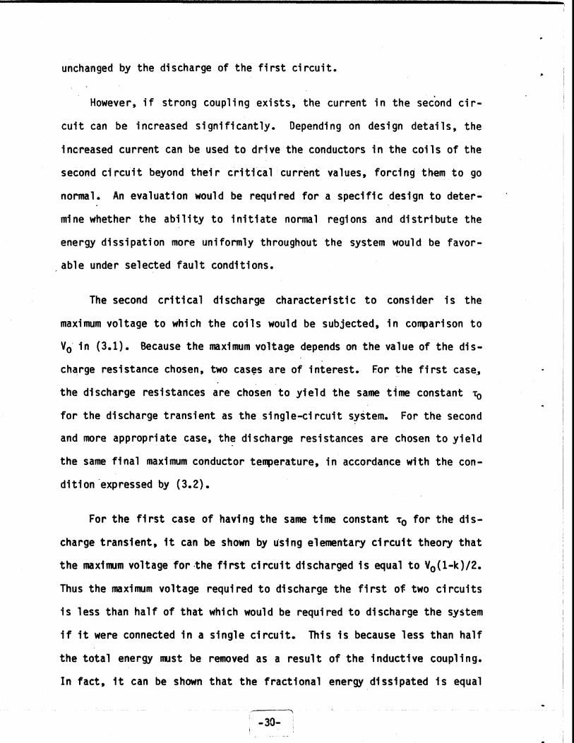
However, if strong coupling exists, the current in the second cir-

cuit can be increased significantly. Depending on design details, the

increased current can be used to drive the conductors in the coils of the

second circuit beyond their critical current values, forcing them to go

normal. An evaluation would be required for a specific design to deter-

mine whether the ability to initiate normal regions and distribute the

energy dissipation more uniformly throughout the system would be favor-

able under selected fault conditions.

The second critical discharge characteristic to consider is the

maximum voltage to which the coils would be subjected, in comparison to

Vo in (3.1). Because the maximum voltage depends on the value of the dis-

charge resistance chosen, two cases are of interest. For the first case,-

the discharge resistances are chosen to yield the same time constant T0

for the discharge transient as the single-circuit system. For the second

and more appropriate case, the discharge resistances are chosen to yield

the same final maximum conductor temperature, in accordance with the con-

dition expressed by (3.2).

For the first case of having the same time constant To for the dis-

charge transient, it can be shown by using elementary circuit theory that

the maximum voltage for -the first circuit discharged is equal to V0 (1-k)/2.

Thus the maximum voltage required to discharge the first of two circuits

is less than half of that which would be required to discharge the system

if it were connected in a single circuit. This is because less than half

the total energy must be removed as a result of the inductive coupling.

In fact, it can be shown that the fractional energy dissipated is equal

-30-

to the normalized maximum discharge voltage for the first circuit. This

can be expressed as

(Eo - E)/Eo = V/Vo (3.4)

where E is the energy remaining after discharge of the first circuit.

If the second circuit was discharged with the same time constant to,

the required maximum voltage would be VO/2. This is assumed to occur

after the first circuit is fully discharged and opened so that there is

no induced current during discharge of the second circuit. The option of

leaving the first circuit closed will be considered in future work.

The case which requires the same final maximum conductor temperature,

Tf, is a more appropriate design condition. It can be shown that the max-

imum voltage for the first circuit discharged is equal. to Vo(1-k)/2,- the

same as in the first case. This is shown plotted as the Circuit 1 curve

in Fig. 3.1, where the maximum discharge voltage is normalized to V0 . Note

that this curve also represents the fractional energy dissipated.

However, when discharging the second circuit, a smaller discharge

time constant is required to limit the temperature rise. A higher maxi-

mum voltage of Vo(1+k) 2 /2 is therefore required. This is shown plotted as

the Circuit 2 curve in Fig. 3.1, again normalized to V0. As shown in the

figure, this may be either greater than or less than the maximum voltage

required for discharge of the single-circuit system, depending on k. The

time constant for this case is given by rO/(1+k)2.

A summary of the discharge characteristics for the two-circuit sys-

tem is given in Table 3.1.

-31-

0'0

0'0

'C

EE

K

E0

2.0

1.5

1.0

0.5

0( 0.6 0.8


Normalized maximum discharge voltage as functionsof the coupling coefficient for a system havingtwo circuits.

-32-

0.2 0.4F 1.0

Fig. 3.1

M

Circuit 2

Circalt I

Table 3.1 Characteristics of Two-Circuit Systems

PARAMETER CIRCUIT 1 CIRCUIT 2

Normalized Current, i/ioinitial value 1 1after discharge of 1 0 1+kafter discharge of 2 0 0

Normalized Max. Voltage, V/Vofor T = (1-k)/2 1/2for Tmax Tf (1-k)/2 (1+k)2/2

Normalized Time Constant, T/T0for Tmax Tf 1 1/(1+k)

3.4 Discharge of Three-Circuit Systems

Consider the same system of 2N TF coils described in the previous

section. However, it is now required that 2N be a multiple of 3 so that

an equal number of identical coils can be included in each of three cir-

cuits. The first circuit will contain the first, fourth, .. , 2N-2nd coils,

the second circuit will contain the second, fifth, .. , 2N-1st coils, and

the third circuit will contain the third, sixth, .. , 2Nth coils. If all

circuits carry an initial current io, then prior to a discharge the condi-

tions are identical to those of the single-circuit system. The analysis is

similar to that for the two-circuit system. Because of the identical coils

and symmetry, the self inductances of each of the three circuits are equal

(L1 = 2 13 1), the mutual inductances are equal (M12 = M21 = M13 =

M31 = M23 = M32 = M), and the coupling coefficients are equal (k12 = k21 =

k13= = =k23 k32 = k = M/L).

In addition to the circuit complexity inherent in the three-circuit

system, there are several features which should be noted. First, one has

-33-

the option of discharging all three circuits sequentially, or of dis-

charging two. circuits simultaneously. The results for a sequential dis-

charge are described herein, as are the results for a simultaneous dis-

charge of Circuits 2 and 3 following the complete discharge of Circuit 1.

The second basic feature which should be noted is that when one cir-

cuit has been discharged but two remain charged, azimuthal symmetry no

longer exists. In traversing the toroid azimuthally, the pattern is: off,

on, on, off, on, on, etc. This asymmetry leads to out-of-plane forces.

The results of an analysis of these forces using an approximate model of

the TF coils are included.

3.5 Discharge Currents and Voltages (3 Circuits)

Discharge characteristics for the three-circuit system are summa-

rized in Table 3.2. These include normalizedcurrents, maximum voltages,

and discharge time constants, all expressed as functions of the coupling

coefficient, k. Again, discharged circuits are assumed to be fully dis-

charged and open circuited to avoid induced currents when the remaining

circuits are discharged.

Normalized currents in Circuits 2 and 3 following discharge of Cir-

cuit 1 are increased by the same amount, as shown in Table 3.2. This is

due to the inductive coupling and symmetry of the configuration. The

amount of the increase, however, is less than that which occurs in the two-

circuit system for a given coupling coefficient. Therefore, there is more

flexibility available for choosing whether or not to use this inductively

driven current increase as a mechanism for initiating normal regions to

distribute the energy dissipation more uniformly throughout the system.

-34--

For the maximum voltages, three cases are summarized in Table 3.2:

(1) sequential discharges with T = To, (2) sequential discharges with

final maximum coil temperatures equal to Tf, and (3) discharge of Circuit

1 followed by the simultaneous discharge of Circuits 2 and 3, with all hav-

ing final maximum coil temperatures equal to Tf. The assumptions associ-

ated with equation (3.2) are used to establish the conditions required to

obtain Tf. Note that Tf is the same value, if (3.2) is satisfied, but the

actual value is unspecified in this analysis because it depends on other

parameters which are not discussed herein, such as the conductor design

details.

Table 3.2. Characteristics of Three-Circuit Systems

PARAMETER CIRCUIT 1 CIRCUIT 2 CIRCUIT 3

Normalized Current, 1/10initial value 1 1

1+2k 1+2kafter discharge of 1 0

1+k 1+k

after discharge of 2 0 0 1+2k

after discharge of 3 . 0 0 0

Normalized Max. Voltage, V/Vo(1-k) (1-k) 1

3(1+k) 3 3

(1-k) (1-k) 1+2k 2 L 22for Tmax = T ------- --

3(1+k) 3 1+k! 3

(1-k) 1 1+2k 2 1 1+2k 2for Tmax = Tf and discharge - - --of 2 and 3 together 3(1+k) 3 1+k 3 1+k

Normalized Time Constant, T/T 0 71+k\2 1)2for sequential discharge 1 --- ----

~1+2k/12

for discharge of 2 and 3 1+ktogether 1 ---- -

-35-

Plots of the normalized maximum discharge voltages are given in Fig.

3.2 as functions of the coupling coefficient for Case 2 (sequential dis-

charges with- Tmax = Tf) and Case 3 (discharge of Circuit 1 followed by

simultaneous discharge of Circuits 2 and 3, all with Tmax = Tf). Note

that the Circuit 1 discharge is the same for both cases. Again,. consis-

tent with (3.4), the fractional energy dissipated during discharge of Cir-

cuit 1 is equal to the normalized maximum discharge voltage. Figure 3.2

shows that the use of multiple circuits can provide a substantial reduc-

tion in the circuit voltages to ground, particularly if the coupling is

low or if Circuits 2 and 3 are discharged simultaneously when using a

three circuit system.

The normalized time constants given in Table 3.2 are plotted in Fig.

3.3 as functions of the coupling coefficient. Only two curves are needed

because the time constant for the simultaneous discharge of Circuits 2 and

3 is equal to the time constant for Circuit 2 in the sequential dis-

charge, and the time constant for Circuit 1 is To.

3.6 Force Considerations (3 Circuits)

When one circuit of a three-circuit system is'discharged, azimuthal

symmetry no longer exists. This results in out-of-plane forces on the TF

coils. As a means for estimating the rough order of magnitude of these

forces, an approximate model of the TF coils has been analyzed. The

model, described by Boris and Kuckes [2) and Thome and Tarrh [3], consists

of 2N straight current filaments of infinite length carrying currents in

the z direction at the locations of the TF coil inner legs (r = a1 ) and

2N straight current filaments carrying currents in the opposite direction

at the locations of the TF outer legs (r = a2)- If R is defined as the

-36-

3.0

02.5-

0' Circuit 3a 2.0U

2--

E 1.5EK

1.0

Circuits 2 and IE 0.5-

0 circuit 2

CircoltI0

0 0.2 0.4 0.6 081.0


Fig. 3.2 Normalized maximum discharge voltages as functionsof the coupling coefficient for a system having threecircuits, discharged under conditions of eiqual finaltemperatures.

-37- i

1.0

0.8-C

0C

0

00

E

0.2

0.'0.2 0.4 -0.6 0.8 1.


Fig. 3.3 Normalized discharge time constants as functions ofthe coupling coefficient for a system having threecircuits which are discharged sequentially underconditions of equal final temperatures.

-38-

average of ai and a2 , which is the major radius of the toroid, while

(a2-al)/2 = a is defined as the minor radius of the toroid, then the nor-

malized out-of-plane forces on both legs can be expressed analytically as

functions of R/a for various numbers of coils for three-circuit systems.

The results of this analysis are plotted in Figs. 3.4 and 3.5, .which

contain the forces on the inner and outer legs, respectively. These

arise from the radial component of field at the leg locations. In both

plots the normalizing quantity is the centering force on the inboard leg

when all circuits are energized, using the approximate model. When Cir-

cuit 1 is discharged, the out-of-plane force is an attraction between the

coils of Circuits 2 and 3 which increases as the number of coils is in-

creased. As shown in the figures, the out-of-plane force on the inner

leg is < 20% of the centering force, while on the outer leg the out-of-

plane force is < 14% of the centering force.

Note that for the two-circuit system, symmetry is maintained if Cir-

cuit 1 is discharged. Thus the two-circuit system has the advantage over

the three-circuit system of having no net out-of-plane loads due to TF coil

interactions.

3.7 Discharge of Multiple-Circuit Systems

An analysis similar to those presented in the previous sections has

been performed for multiple-circuit systems containing as many as nine

separate circuits. To maintain the simplicity of the analysis, it was as-

sumed that the total number of TF coils was an integral multiple of the

total number of circuits. Thus each circuit in the multiple-circuit sys-

tem is assumed to contain an equal number of identical coils for a given

-39-I

I

0.20

I

3.0I

4.0I

5.0Normalized Major Radius, R/a

Approximate normalized out-of-plane forces on theinboard leg as functions of the normalized majorradius -for -various numbers -of coiia-nsystem- -

having three .circuits.

-4 0-

36

30

- 24

- Number of Coils 12

b..

0

C

0

0

4)

E0

z

0.16

0.12

0.08

0.04

fm~-I

Ii I

1.0

Fig. 3.4

6.0

0.16

Number of Coils .360

0.12- 30

c 24

cIs0 0

a-2o 0.08

= 0.04E

zII

1.0 2.0 3.0 4.0 5.0 6.0

Normalized Major Radius, R/a

Fig. 3.5 Approximate normalized out-of-plane forces on theoutboard leg as functions of the normalized majorradius for variousnuihbAQfcA~ilainasystemhaving three circuits.

case. The discharge characteristics for the first circuit in the multiple

-circuit system are presented. The requirements on, and discharge charac-

teristics of, the remaining circuits are the subject of ongoing systems

analysis.

A computer program has been written to examine the discharge charac-,

teristics for specific cases, based on the analysis. The program has been

applied to the TF configuration given in Fig. 3.6, which is an early ver-

sion of the TFCX TF coils. For this application, from 1 to 8 circuits

were considered. In addition to the 16 coil TF set described in Fig. 3.6,

a 12 coil set was analyzed by using the same dimensions shown in the fig-

ure, but with the ampere turns per coil increased. by the ratio of 16/12.

The self and mutual inductances for a given number of multiple circuits

were obtained by computing the self and mutual inductances for and be-

tween individual coils in the complete set, then collapsing the induc-

tance matrix based on the number of multiple circuits. The general form-

ulation and procedure for this calculation, as well as the analysis of the

discharge characteristics, are available [1] and will not be reproduced

here due to space limitations.

Results of this analysis applied to the TFCX configuration are given

in Table 3.3. Spaces In the table are left blank where the basic assump-

tions on joining coils into separate circuits can not be met. Thus there

are no results for the case of 16 TF coils and three circuits, for ex-

ample, because the 16 coils can not be evenly divided among the 3 cir-

cuits. The discharge characteristics given are for discharge of the

first circuit only.

-42-

4

0 24 6 8

r, meters

L358

0.541

Fig. 3.6 Sketch of a typical TF coil for TFCX, which includes16 TF coils, each having a thickness of 0.541 m.

-43-

Table 3.3. Characteristics of TFCX

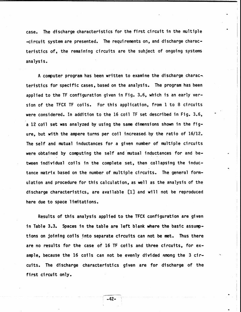
NO. OF NUMBER OF CIRCUITSPARAMETER COILS 1 2 3 4 6 8

Normalized 12 0 1.6 1.3 1.29 1.28 -Current, i/in 16 0 1.74 - 1.36 - 1.35

Normalized 12 1.00 0.20 0.13 0.10 0.06 -Voltage, V/Vn 16 1.00 0.13 - 0.06 - 0.03

Norm. Toroidal 12 0 0.80 0.87 0.90 0.94 -Field, B/Ba 16 0 0.87 - 0.94 - 0.97

The normalized current parameter given is the current in the circuit

adjacent to the discharged circuit, normalized to the current prior to

discharge. The current in the adjacent circuit is given because this is

the circuit most strongly influenced, due to the closer coupling to the

discharged circuit. The most significant current increase occurs for two

circuits, while for three or more circuits the current increase does not

depend strongly on the number of circuits..

The normalized maximum voltage parameter given is also equal to the

fractional energy removed during the discharge of the first circuit, in

accordance with (3.4). As the number.of circuits is increased, the frac-

tional energy removed and the maximum voltage to ground both decrease,

with the most dramatic decrease occurring for two to three circuits in

comparison to one.

The normalized toroidal field parameter is the ratio of the final

average toroidal field to the initial field level. The table indicates

that 80% or more of the initial field level is maintained for the 12 coil

system with two or more circuits when one is discharged, and Lhat 87% or

more is maintained for the 16 coil set.

-44-

3.8 Summary and Conclusions

The use of multiple TF coil circuits has been shown to have advan-

tages and disadvantages. The primary disadvantage is the increased cir-

cuit complexity. While having two circuits may be only moderately more

complex than one, the complexity (and consequent reliability considera-

tions) involved with having three or more circuits is considerably in-

creased. The second major disadvantage of having three or more circuits

is the resulting out-of-plane forces when one circuit is discharged. For

the single and two-circuit systems, there are no unbalanced out-of-plane

loads due to TF coil interactions.

The major advantage of multiple TF coil circuits is the reduction of

maximum discharge voltages to ground. Relative to the single-circuit

system, using two circuits can significantly reduce the discharge volt-

tages, while further reductions can be achieved by using three or more

circuits.

A second advantage of multiple circuits is that one may have the op-

tion of using the inductively-driven coil current increase as a mechanism

for initiating normal regions and spreading the energy dissipation. For

two-circuit systems, it appears that with only moderate coupling the

initiation of normal regions would be unavoidable due to the level of the

increased current. However, with three or more circuits, it appears that

one would have the choice of whether or not to use this mechanism.

-45-


1. R.J. Thome, et al., "Safety and Protection for Large Scale Supercon-ducting Magnets - FY1983 Report", PFC/RR-83-33, December 1983.

2. J.P. Boris and A.F. Kuckes, "Closed Expressions for the MagneticField in Two-Dimensional Multipole Configurations," Nuclear Fusion,Vol. 8, pp. 323-328, 1968.

3. R.J. Thome and J.M. Tarrh, MHD and Fusion Magnets: Field and ForceDesign Concepts. New York: John Wiley, 1982, Ch. 3, pp. 158-160.

-46-

wwwwm

4.0 HPDE MAGNET FAILURE - J.M. Tarrh and H.D. Becker

4.1 Introduction

In December of 1982 a large magnetohydrodynamic (MHD) magnet for the

High Performance Demonstration Experiment (HPDE) at the Arnold Engineering

Development Center (AEDC) suffered a catastrophic structural failure,

which led to brittle-fracture failures in most of the structural compon-

ents, significant displacements (on the order of a meter) of some -of the

magnet iron frame components, and similar deformation of the winding with

some conductor fracture. Our FY83 report contains a detailed description

of the magnet system, a summary of the failures, and the results of a pre-

liminary structural failure analysis.1 This chapter contains a brief in-

troductory summary of the magnet system and cause of failure, and an up-

date of the preliminary analysis to document work performed during FY84.

4.2 Summary

The HPDE employed a large (active bore approximately 1 m square x 7 m

long) iron-bound copper magnet designed to operate in either of two modes:

(1) as a 3.7 T (continuous) water cooled magnet, or (2) as a 6 T (long

pulse) nitrogen-precooled, cryogenic magnet. In either mode, coolant

would flow through conventional hollow copper conductor windings. A uni-

que force containment structure (FCS) was designed for the magnet. An

aluminum alloy (2219) was selected on the basis of thermal considerations

(77 to 350 K operating'temperature range; coefficient of thermal expan-

sion permitting dimensional matching to the coil) and cost.

-47-

Figures 4.1 through 4.3 show, respectively, a photograph prior to the

failure of the magnet including the outer thermal enclosure, the general

distribution of the design Lorentz forces on the coil windings, and the

force containment structure (FCS). Components of the FCS were fastened

together with high strength keys and bolts.

The FCS design analyses identified multiple load paths for support

of the total longitudinal force. The effects of tolerances on the inter-

actions among FCS components increased the complexity of the structural

analysis. Although the design was conservative with respect to support

of the longitudinal loads, the analysis overlooked the effects of trans-

verse loads (in the saddle region) on the longitudinal force support ele-

ments.

Figures 4.4 and 4.5 graphically depict the effects of the transverse

saddle loads on the longitudinal tension members (LTM) and on the collars.

As a result of these transverse loadings, the calculated combined stresses

in the fingers of the LTM (where they are notched to penetrate the face-

plate) were on the order of 130 ksi which is well in excess of the mea-

sured ultimate strength of the 2219 aluminum alloy (at 77 K). These

stresses occurred at a field level of 4 T, which is approximately half the

design load. Stresses in the collar fingers were on the same order.

The magnet failed at a field level of 4.1 T as a result of design de-

fects that were not detected during the FCS design analyses. For a more

detailed discussion of the design and analysis of the failure, including

a discussion of failure scenarios, see Reference 1.

-48-

a .

4*

tm

&--

-L.

-49-

-49-

0

.~~ Lai.

4)

LA6.-0

co

C-)

At 0

INI

CDCcv 0

U_-

it 0. C0~cw% to

Ln I-

0-4-50-

a CDI

ELL

4J

4-)

CL

U

cn.

00

COLLAR

SIXE PLATE SIDE BEAMS

-- LONGITUDINALLTM FINGERS - - TENSION MEMBER

FACE PLATE - -- -

- COIL

B = 0 NO DEFLECTIONS

B +- 4 T NO COLLAR FAILURE

B + 4 T AT COLLAR FAILURE 4A t

FigWe 4,4 Exaggerated depicdion of LTM-related deflectionsat the magnet midplane

-52-

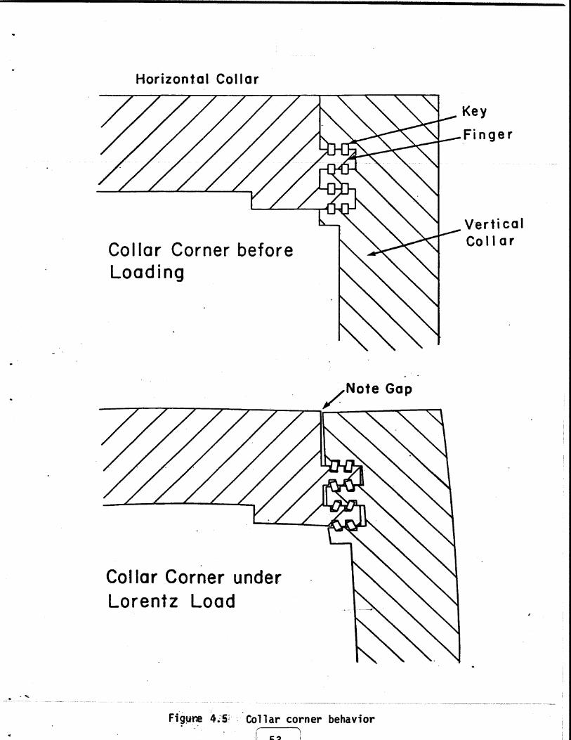
Horizontal Collar

Collar Corner beforeLoading

Note Gap

Collar Corner underLorentz Load

.-,Key_Finger

VerticalCollar

Figure 4.5 Collar corner behavior

I-5 3-

4.3 Update of Preliminary Structural Failure Analysis

During FY84, key elements of the preliminary failure analysis were

reviewed and updated. The principal focus of the effort was to recalcu-

late the magnetic fields and forces using up-to-date tools and techniques

since the preliminary failure analysis had been based on the original de-

sign calculations which were performed during the mid-1970's.

To recalculate the magnetic fields and forces, a current level cor-

responding to a peak on-axis field of 4 T was used, since this was approx-

imately the field strength (and force level) at which failure occurred.

A three-dimensional filamentary model of the coil was constructed using a

2 x 2 matrix of filaments per coil. The coil model closely approximated

the actual coil configuration in that the bore taper was accurately in-

cluded in the model. Two detailed filamentary models of the iron return

frame were also constructed. These were three dimensional in that they

were of finite length. However, the taper was not included in these

models, one of which consisted of the dimensions of the iron at the inlet

end of the magnet, while the other used the outlet end dimensions. The

differences in fields between these two iron models were not significant,

particularly since the fields (and forces) on the coil outlet end turns

were of primary interest. The coil outlet end turn fields and forces were

of primary interest because the structural failure was initiated in the

outlet end turn region of the magnet.

Separate models of the coils and iron were used so that thL cffects

of the iron on the total coil forces could be determined accurately. This

was necessary so that force scaling with current level could be easily ac-

complished, because the total force on the coil over a given region of the

A;54-

coil can vary more (or less) strongly than the square of the current level

depending on whether the field within the coil due to the iron subtracts

from (or adds to) the field due to the coil itself. This is true because,

above saturation, the force on the coil due to the iron is approximately

directly proportional to the current level, whereas the force on-the coil

due to the coil itself is directly proportional to the square of the cur-

rent level. This can be expressed as

F = k12 + IBi (4.1)

where

F = total force on coil region

I = current level

K12 = force on coil due to coil

IBi = force on coil due to iron

k,Bj = proportionality constants

and the negative sign is used if the iron field subtracts from the coil

field (within the coil), while the positive sign is used if the iron field

adds to the coil field (w-ithin the coil). Because the first term in this

equation typically dominates in these configurations, it can be shown that

the negative sign leads to a total force which varies more strongly than

the square of the current level, while the positive sign leads to a total

force which varies less strongly than the square of the current level.

Using these models to determine the forces in the outlet end of the

coil y-ielded the following results (values are forces expressed in MN at

a current level corresponding to a peak on-axis magnetic field of 4 T):

-5 ------

AXIAL LATERAL VERTICAL

Coils Only 17.3 2.5 2.5Coils and Iron 16.4 2.9 3.5

Appropriate scaling of these forces with current level allows comparison

with the original design force calculations summarized in Fig. 4.2. This

was a valuable process, as it uncovered a mistaken assumption that had

been used for the preliminary structural failure analysis. Because the

design peak on-axis magnetic field of the magnet was 6 T, it was assumed

that the forces of Fig. 4.2 corresponded to a 6 T field condition. The

presentations in the original references were unclear on this point. It

was discovered, however, that the Fig. 4.2 forces in fact correspond to a

peak on-axis magnetic field of 6.8 T rather than 6 T. The 6.8 T field

level was a performance goal in effect during the early stages of the mag-

net design. - This goal was relaxed to 6 T during the design process, al-

though the force and coil pressure distributions that were presented in

the original references (the final design report) remained unchanged, cor-

responding to the current level for a. 6.8 T peak on-axis field. (This

discrepancy has been promulgated in several places. 1-3 Consequently, the

coil forces used in our preliminary structural failure analysis were in

error. The force values were scaled from 6 T to 4 T assuming that they

were directly proportional to the square of the field, when in fact they

should have been used closer to 0.30 based on the more recent calculations

described hereinabove.

The actual force levels at failure were therefore considerably less

(by a third) than those used for our preliminary structural failure anal-

ysis. However, we have reviewed the failure analysis in view of the re-

duced force levels and find that while the specific numerical values

-56-

change, all of the conclusions of the preliminary failure analysis remain

valid since the maximum stresses would be of the order of 130 ksi which

exceeds the ultimate strength of 2219 aluminum alloy.

A final comment on the significance of- this failure is in order.

Subsequent to the failure, the structure was considered beyond repair.

The coil windings were considered to be repairable without prohibitive

time, effort, or cost assuming reduced performance requirements (single

mode operation only, pulsed from room temperature). The magnet could have

been rebuilt without an infusion of substantial additional funds by per-

forming the repair and rebuild using the anticipated future operating

funds slated for the facility. The experiment was unique in size and field

strength, and at the time of the failure had just begun to obtain signifi-

cant data on new MHD phenomena (the so-called magnetoaerothermal instabi-

lity), which may be of significance to the overall development and commer-

cialization of MHD. The MHD community was therefore strongly in favor of

repairing the magnet so that these unique experiments could continue.

Nevertheless, the magnet repair was in fact not initiated, and at this time

the facility remains shut down and mothballed with all of the personnel

disbanded to work on other (non-MHD) projects. These facts underscore the

significance of this failure and the criticality of the magnet system as a

component to those large scale technologies which require them.

Additional comments on this magnet failure (among others) were in-

cluded in a workshop on magnet failures held during the MT-8 Conference

in Grenoble. 4

-57-

4.4 Reference for Section 4

1. R.J. Thome, R.D. Pillsbury-, Jr., W.G. Langton, et al., "Safety andProtection for Large Scale Superconducting Magnets -- FY83 Report,"MIT Plasma Fusion Center, Cambridge, MA, December 1983.

2. R.M. James, et al., "Investigation of an Incident During Run Ml-007-018 MHD High Performance Demonstration Experiment (PWT) onDecember 9, 1982," ARVIN/CALSPAN Field Services, Inc., AEDC Divi-sion, Arnold Air Force Station, TN, April 1983.

3. H. Becker, J.M. Tarrh, and P.G. Marston, "Failure of a Large Cryo-genic MHD Magnet," presented at the MT-8 Conference, Grenoble,September 1983, published in Journal de Physique, Colloque Cl,supplement au n0 1, Tome 45, Janvier 1984.

4. P.G. Marston, et al., "Magnet Failure Workshop," Journal DePhysique, Colloque Cl, supplement au no 1, Tome 45, Janvier 1984.

-58-

5.0 TFCX MAGNET OPTIONS - R.J. Thome, U.R. Christensen, M. Pelovitzand W.G. Langton

A preliminary study of fault load conditions was carried out for three

of the options under consideration for TFCX. The specific characteristics

of the cases are defined in this chapter and the alterations in electromag-

netic loads under specific TF and PF fault conditions are compared. A

large number of faults were evaluated, but the study was by no means com-

plete. In many instances, loads are nontrivial, but are believed to be

manageable through proper structural and protection circuit design. They

indicate a need for ultimate specification of a list of credible faults

and their consideration in the design process.

5.1 Option Definition

The TFCX preconceptual design effort defined four options' which

could satisfy the same physics mission. They consisted of machines using

copper or .superconducting TF coils based on "nominal" or "high perfor-

mance" design criteria. In all cases, the PF coil system was supercon-

ducting. Early in the effort, a hybrid system consisting of a nested set

of copper TF coils within a set of superconducting TF coils was also con-

sidered.

This study was initiated before the last TFCX preconceptual design

iteration; hence, the specific machine characteristics are somewhat dif-

ferent from those in the design reports.1 The features of the three sys-

tems are summarized in the elevation views in Fig. 5.1 which shows the TF

winding outline and PF coil cross sections for one quadrant of the machine.

All coil systems are symmetric relative to the z = 0 plane and consist of

TF coils in planes equally spaced around the z axis and PF coils coaxial

with the z axis. The top figure has a maximum toroidal field of 8.45 T

-59-

Comparison of TF Coil Characteristics

TFCX - Cu4250 MJ

4-.38

Radial Coord. (m)

Trcx - uIEncomouvimlNG

E =

MAT =

F =C

F =v

r

S.

S.= 7460 MJ

= 5.36

= 140 MN

= 74.6 MN

= 114.6 MN-m

-

-6

0-

a.

a.

ii.I a.

bore \, 4.4 x 6.4 m(% Hi Perf SC)

C.

Rad'ial Coord. (m)

TFCX - YBRIO

E = 3280 MJ

-3.88 + 1.43 5.31

= 68.0 + 2.8 = 70.8 MN -6

= 32.1 + 18.1 = 50.1 MNS

= 61 + 12.6 1 73.6 MN-m-

S.

S.

S.

U.

S.

I.

a.. 1.

Axial Cooro. (mi

0. a.

bore " 3.4 x 4 m

8.45MT

S.

bore , 4.1 x 6 m(o nom Cu)

69.4

42.3

67.8

MN

MN

MN-m

U

-.

S.

a.

3.

M

E

MAT

F.cF

V

r

MAT

F

FV

rCu

8.0 T

8.0 T

1 0 T

Fig. 5. 1 -

11.

at the winding and is similar to the "nominal" copper design for TFCX;

the center figure has a maximum field of 10 T and is similar in size and

TF level to the "high performance" superconducting. design although the

plasma current and PF system were not yet optimized at this stage; the

lower figure is a "hybrid" of 16 copper coils nested in 16 superconducting

coils with a maximum field of 8.0 T and was under consideration early in

the TFCX design effort, but ultimately discounted as an option. The fig-

urie also summarizes selected characteristics under usual operating condi-

tions, that is: E = stored energy in the TF coils; MAT = megampere-turns

per TF coil ; Fc = net load per TF coil toward the machine axis (centering

force); Fv = vertical load tending to separate the top half of a TF coil

from the bottom half (sum of tension in inboard and outboard legs at the

mid-plane); and Mr = overturning moment on a TF coil about the r axis due

to the interaction of the TF coil. current with the poloidal field. The

figures are drawn to scal-e and indicate the similarity in machine size;

note, however, that the stored energy and loads differ by factors of the

order of two. This is primarily due to the differences in field level,

bore size and average radius. The differences in overturning moment are

also due to these factors and to differences between PF systems.

Figure 5.2 summarizes the megampere turns in each of the PF coils at

the start of burn and with the plasma current indicated. Vectors are

drawn to scale on each PF coil to illustrate the local load per unit coil

circumference due to the PF system and the plasma. These loads are axially

symmetric and uniformly distributed. -In addition, the PF coils (ring

coils in particular) experience a spatially periodic load (not shown) due

to the ripple and stray field from the toroidal field coils.

-61-

Fig. 5.2 - EM loads per unit length on PF coils at start of burnwith plasma; forces are to scale and values are megamp-turns in PF coils

TFCX-Cu

5.15 MA

5.q15

7 *7

- 0

3. S.

force scale

10 MN/m

0.

RedieI Coord. (m)

TFCX - 8UPEPCONDUCIING

9.34 MA

9.3- 6.16

.

3

7.71 .

RedieI Coor2. (m)

TFCX - ITaRID

0.

Rx e a I Cooro. (m)

-62-

a.

E

a.

3.

3.

S.

S.

5. r--6

0e

a.a.

S

00

0

12.2 MA

6.0 -7.0

.. 3.07

6.

I-

1. 0.

- 1.

2.

The OH solenoid in the top figure consists of two coils with the MAT

distributio6 shown so that there are 5 coils with mirror images below the

z = 0 plane in the top system. There are 4 PF coils (8 total) in the super-

conducting system in the center sketch and 5 PF coils (10 total) in the hy-

brid systent in the lower figure. The machines are close to the same size

and represent different stages in three designs on the way toward satis-

faction of the same physics mission, but the load patterns are similar and

of the same order of magnitude although differences of order 2-3 are evi-

dent. These differences between options as well as those for the TF coils

are partially due to the fact that all three cases have not been opti-

mized to the same level. They all represent load levels which are fea-

sible from the engineering standpoint.

5.2- Fault Conditions

The only fault conditions considered in this preliminary study were

changes in electromagnetic loads due to abnormal current distributions in

the coil systems. The conditions illustrated in Figs. 5.1 and 5.2 were

assumed to be the usual or "normal" operating conditions. Excursions

from these current distributions among coils were then postulated in the

form of discharging one (or more) coils and the plasma, then finding the

new coil currents assuming their circuits maintained a constant flux con-

dition. The new currents were then used to recalculate the load patterns

and to ratio the resultant forces to their counterparts under usual operat-

ing conditions. The ratios then indicate when a load exceeds the usual op-

erating conditions (i.e.- ratio > 1) or when it reverses direction relative

to the usual condition (i.e. ratio < 0).

-63-

5.2.1 PF Fault Influence on PF Coils

The first class of conditions considered in this part of the study

assumed that each PF coil pair (one above and one below the z = 0 plane)

was in an independent circuit since it would be likely that independent

control for plasma shaping and other experiments would be necessary. One

circuit (and the plasma) are then discharged to zero because of a fault in

that circuit and the others are assumed to maintain constant flux. This is

a symmetric PF coil fault since a pair of coils is discharged and field

symmetry with respect to the z = 0 plane is retained. A typical result is

illustrated in Fig. 5.3 which shows one of the ring coil pairs (shaded)

discharged to zero current. The number adjacent to the other coils is the

ratio of the final to initial current in that circuit based on a constant

flux assumption. In all three cases, discharging the coil shown leads to

current increases in the inboard coils and a decrease in the outboard

coils. The latter occurs because the outboard coils carry a current of op-

posite sign under usual conditions (see Fig. 5.2). Two questions now

arise: (1) are the individual coil loads now greater than or reversed in

sign relative to those under the usual condition, and (2) is the change in

current level sufficient to induce a normal region in a coil which is still

"on" because its critical current is exceeded?

Cases were considered where each of the circuits was symmetrically

discharged as described earlier and two sample cases were considered where

only one coil (e.g. - above the z = 0 plane) was discharged to gain insight

into an asymmetric fault. For each case and each coil, the ratio of final

to initial current was calculated together with the ratios of final to ini-

tial radial and axial forces. Initial states were as defined in Fig. 5.2

and results are summarized in Tables 5.1 and 5.2 with coils denoted as in

Fig. 5.4.

-64-

Fig. 5.3 - Typical case of symmetric PF coil fault-and PF circuit current changes

initial I = 0.961a.

0.0

1.51 0.79

1. a.

M rf [1.24r TF

Mrf = 1.52r

TF

a.

Radial Coord. (m)

rCx - HY5I'O

Mrf - 1.76

r |TFSC

m -f 0.74r

TFCu

6.

R eaI Ceora. (m 6-65-

-0final I0.0

1.38~

1.05

105

Radial Coord. (ml

Trcx - aurencoNDUCIING

a

S..CC

Ca.

3.

U a

U

a-00

C.,

C

S.

S.

I.

I.

2.

3.

.

0.0

2.20 0.81

1.23

I. - -Fr

0

0C..

7;

a. (a. 6.--a.,

Fig. 5.4 -

a

I-.00

C

I.

5.

9.

a.

3.

3.

a --- .

A

PF coil designations for fault studyresponses (Table 5.1)

TFCX - Cu

r. 0. a.

Radial Coord. in)

TFCX - SUPCnCOwOUCI1NG

9.

Radial Coord. (m)

rFCX - HBriO

1. G.

Rxiel Cooarc. (ml

-66-

a.

4.

7;I.

Z.

3.

'AU.

U. 1. t.

S.

..

S-.

a.

3.

a.

S

0:

a. 0.

C

B '

, ,

FB

A

FB

TABLE 5.1

RATIO OF NUMBER OF "LARGE" EXCURSIONS* TO NUMBER OF FAULTS FOR PFINTERACTIONS WITH PF COILS

COIL

A' AFAULT FACTOR

DESIGNATION

B' B C D

COPPER

SUPERCONDUCTING

HYBRID

FR

Fz

IR

FR

Fz

IR

FR

Fz

IR

0

4/5

1/5

NA

NA

NA

NA

NA

NA

0

4/5

2/5

0

3/52/5

1/6

1/6

4/6

NA

NA

NA

NA

NA

NA

3/6

3/6

4/6

0

3/5

1/5

0

2/51/5

1/6

3/6

2/6

2/50

1/5

2/50

1/5

3/60

1/6

0

4/50

0

4/50

-0

5/60

NA = Coil not in system (See Fig. 5.4).* = "Large" Excursion, implies a case where a ratio was

greater than unity or less than zero; the corres-ponding range of the ratios in each case is given inTable 5.2.

5 = 5 symmetric for Cu optionNUMBER OF FAULTS =5 = 4 symmetric + 1 asymmetric for SC option

6 = 5 symmetric + 1 asymmetric for hybrid option

-67-

SYSTEM

S

0

0 a 0

'-4

'-4

C"iC%

0o

C"j0D

'-4

C"j

0-

'-D

C'DLi

C%J

0c)

. 0D

C',I,

C"j

0

-O m

C"

o a

0

CCD

00 ~

C% C% C% .

U) ON* a

,4 1:

u; %S Sl

*l to 0

V-4 P- V-

C',

I-o

V-4

wN w ce N~ cz =NU- U- . - U.. La. 14 U- L" *-

CD

5-

Li

c-

a-a.0C-,

C%C')

LAJ-j

Q

u.

2MQ-

-LJ0=

05-C-,

Li.

I-

-J

SJ-

zA-

U)

4-)

C1

4-.

4J)

Three ratios or fault factors were evaluated. In summarizing re-

sults in Tables 5.1 and 5.2, excursions in forces or currents which were

greater than 10% (i.e. - fault factor > 1.1) were considered "large" as

well as cases where force directions reversed (i.e. - force fault factor

< 0). The former implies a potential problem in terms of exceeding the

critical current or structural capability and the latter implies a rever-

sal in load direction relative to the usual case (Fig. 5.2). The coil de-

signators in Table 5.1 correspond to those in Fig. 5.4 and the table sum-

marizes the number of "large" excursions in force or current experienced

by the coils relative to the number of faults considered. Table 5.2 gives

the range of the ratios for the calculated faults in each case. Since the

number of fault conditions was limited and the three systems were not ini-

tially optimized to the same level, the systems should not be compared, but

certain common trends are-indicated:

(a) all coils except the outboard ring coil exper-ienced substantial changes in current relativeto their operating levels.

(b) coils can experience loads which are signifi-cant multiples of their usual loads or loadreversals under selected conditions.

Although the excursions are large, they should be considered man-

ageable from the design standpoint provided a sufficiently thorough fault

condition analysis is ultimately performed and protective circuits are em-

ployed if required.

Sixteen fault conditions were considered relative to usual operat-

ing conditions at start of burn. Other points in the start-up, burn and

shut-down scenario require analysis at a later stage in design and could

yield fault factors which meet or exceed the ranges given. The process

is-stratghtforwar4, but tedious and requires development of codes which

-69-

can allow a large number of cases to be treated without the interactions

now required for transcription and reduction of inputs and outputs.

5.2.2 PF Fault Influence on TF Coils

Under usual operating conditions in a symmetric system, the PF in-

teracts with the TF coils such that each TF coil experiences out-of-plane

forces which have no resultant, but which generate a moment about the r-

axis in its plane. This is illustrated in the top sketch in Fig. 5.5 and

in the event that a symmetric PF coil system fault occurs, the magnitude

of this moment will change. For example, Fig. 5.3 gives the ratio of the

overturning moment on a TF coil for the PF coil fault indicated to the

value of the overturning moment under usual conditions. As shown, the

ratios are typically of order 1 to 2. These moment ratios were found to

exceed unity in five out of the fourteien symmetric fault conditions con-

sidered.

In the event that an asymmetric PF coil fault occurs, the out-of-

plane forces will change such that the overturning moment discussed

earlier will change and the forces will have a resultant through the ma-

chine axis. This is shown in the center sketch in Fig. 5.5. There is,

therefore, no net moment about the machine axis, but the resultant is

equivalent to the case in the lower sketch which shows a net out-of-plane

force at the average coil radius and a z-directed moment about an axis

parallel to the z-axis and located at the average radius. To illustrate

the relative magnitude of this type of fault, two sample cases with asym-

metric PF faults were calculated. They indicated that the resultant out-

of-plane force was a few percent of the net centering force under usual

operating conditions and that Mza as defined in the lower sketch in Fig.

5.5 was 25-35% of Mr under usual conditions. Loads of this magnitude are

nVia --and indicate the need for considering a-broa-drange of fatrlts

a~tosmejater time however, they are not so large as to imply lack of

Fig. 5.5 - Illustration of PF interactions with a TF coil.

- symmetric PF produces momentM under usual conditionsr

- symmetric PFchanges M

r

coil fault

TF coil

r

- asymmetric PF coil faultchanges r to Mra

- asymmetric PF coil faultgives net out-of-planeforce through z - axis

resulting in no momentabout the z-axis

Fop

ra

r

- above figure is equivalent toresultant F at (rI+r2)/2opand a moment - F (rl+r 2)/2

opbut the choice of radius toF P can be arbitrary

-71-

z

rz

Fop

z

Mza

N

I

I

I

Mra

r

feasibility. As in the previous section, a sufficient number of faults

was not investigated to indicate a trend between options nor were the in-

itial designs optimized. However, results imply a need for thorough fault

analysis and definition of load excursions for consideration in the design

process.

5.2.3 TF Fault Influence on TF Coils

The magnitude of fault loads in the TF system were estimated for

one case in the TFCX Cu option. This was an extreme situation in which one

coil was completely discharged while the others altered their current to

maintain constant flux linkage. The result is that:

(a) the coil adjacent to the discharge coil experiencesa net out-of-plane force comparable in magnitude tothe centering force it experiences during usual op-eration;

(b) the current in the remaining coils increases about7%;

(c) the centering force on the coil adjacent to thedischarged coil rises less than 1% and the totalvertical load in the coil legs at the mid-planefalls to about 70% of the value before the load.

Item (a) is by far the most significant since a TF coil in a symmetric

PF experiences no net out-of-plane loads under usual conditions. However,

this type of result is common among options, so it will require further

consideration during design when it must be determined to be either: (1) a

condition with vanishing probability because of system configuration; or

(2) an allowable overload for a specified number of fault cycles.

-72-

5.2.4 TF Fault Influence on PF Coils

The change in loads on the PF coils due to TF coil faults were not

calculated for the TFCX options. In general, 2 a TF coil system fault which

is symmetric relative to the machine axis will alter the load distribution

and the associated local bending moments on a PF coil. If the TF system

fault is asymmetric, a PF coil could also experience a moment tending to

rotate it about a line which passes through the machine axis and the fault-

ed coil, as well as a net force in its plane.

5.3 Summary

This study represents the first step fault analysis for TFCX and

indicates that ratios of fault currents and loads under selected condi-

tions are nontrivial; however, no fundamental advantage was apparent

among the copper, superconducting and hybrid .options considered. Th.is

was partially due to the limited number of cases (17) considered, -parti-

ally due to the fact that fault factor ratios are probably similar in

devices of similar size and field level, and partially due to the differ-

ences in level of design detail available for the cases considered. In

general, it will be necessary to evaluate a much larger number of cases at

a later stage in the design. The process is straightforward, but the

codes required for systematic evaluation, transcription of inputs/outputs

and summarizing fault factors need further development.


1. "TFCX - Preconceptual Design Report - Vol. I, II," PPPL, F-Axxx-8407-006, F-Axxx-8407-007, July 1984.

2. R.J. Thome, J.M. Tarrh, "MHD and Fusion Magnets:Field and Force De-sign Concepts, Wiley, 1982, p. 198.

-73-

6.0 SAFETY RELATED EXPERIMENTS

6.1 ICCS Small Football Coil - J.V. Minervini and P. Rezza

A small football coil made of internally-cooled cabled superconductor

(ICCS) was constructed in 1983 and safety related experiments were per-

formed in March 1984. The coil was originally constructed to measure the

effects of strain, cyclic fatigue, and conductor motion on the conductor

characteristics including critical current and stability. The tests de-

scribed here were performed to investigate failure mechanisms in coils

wound with ICCS conductops.

The coil and conductor were described in the FY83 Report 1 but the

characteristics are repeated here for convenience. The conductor was made

up of a 27 strand cable of bronze matrix Nb 3Sn in a sheath of JBK-75

superalloy. The conductor characteristics are summarized in Table 6.1 and

a photograph of the conductor cross section is shown in Fig. 6.1. The

coil and mandrel are shown in schematic in Fig. 6.2. The photograph in

Fig. 6.3 shows the coil with the side support plates in place but for the

tests described here the plate on the side opposite the terminations was

removed. This was done in order to increase the chance for failure.

The experiments were performed in a uniform DC background field pro-

vided by the 6-inch bore Bitter magnet at the Francis Bitter National Mag-

net Laboratory. The test consisted of three parts:

(1) measurement of critical current(2) measurement of quench voltage and pressure(3) attempt to quench to failure of the winding

TABLE 6.1

SMALL FOOTBALL COIL CONDUCTOR PARAMETERS

Material

Cu: Noncopper Ratio

Void Fraction

Sheath

Sheath Wall Thickness

Sheath Dimensions

Strands

Strand Diameter

Nb3Sn, Copper Stabilized

1.8

32%

JBK - 75

0.015 in. (0.38 mm)

0.192" x 0.192" sq. (4.88 mm sq)

27

0.7 mm

4

-75-

4-)u

0 44.)

04 -U)I

44.0L

-76-

bus

HydraulicI input /output

Scale:

I inch

ICCS Conductor

I "football" Winding/SuMandrel

- Conductor Groove

N A A

pport

-+-1

Sect. A-A

ConductorReturnLoop

Figure 6.2 Outline of mandrel forsmall footbal Wtest.

-77-

C

IN:0

~1

-78-

-x

Mr

C

30.

'4-)

o o

U) U

Sa))O

0 '

4-

-4)

U-

(UU

0 to

0M 0

4-

U.

A schematic of the helium flow configuration is shown in Fig. 6.4

and a schematic of the instrumentation set-up is shown in Fig. 6.5.

6.1.1 Measurement of Critical Current

The critical current as a function of field was measured in order

to compare with data taken previously. Apparently the critical current

varied somewhat between experiments and so the Ic versus B measurements

were taken to get a datum. The results are shown in Fig. 6.6. The data

of this experiment (3/14/84) compare very well with the most recent data

taken on 11/29/83 even though one support plate had been removed for this

test. Both sets of data are slightly higher than that taken on 11/25/83.

This is probably not significant. In all cases the data were recorded on

an x-y recorder using an electric field criterion of 1.5 vV/cm to deter-

mi.ne the critical current.

6.1.2 Measurement of Quench Voltage and Pressure

A principal goal of this test was to measure pressure in the coil

during a quench. The peak quench pressure could have a significant impact

on any magnet design since it could determine the maximum helium flow

length and if the coil is connected to a refrigerator, the sudden expulsion

of high pressure helium could have serious consequences for the turbo-ex-

pander. These units are delicate and expensive and would have to be pro-

tected from pressure surges by check valves and expansion chambers.

Of course the ultimate coil failure would be caused by the pressure

bursting the conduit or one of the many joints in the helium flow path.

The maximum quench pressure can be estimated from an expression given by

Miller and Lue 2:

-79-

Pressure Relief ValveTransducer Vapor

CooledLeads

Location ofHelium Look

FlowMeter Pressure Pressure

MeteringVnlvv

Pressure- Regulator

He Gas

Cylinder

-Hoot Exchanger

Initial LHe Level

+ -Dewar

-Bif liar Coll

Fig. 6.4 Schematic of helium flow path for small football Coil test.

-80-

) .

Houstonx- y Recorder

or Supply-

Preston Amp BiomationGaina10

0 Channel I

HomemadeAm Am Channe 2

GaOin 50,000

Preston A

S

Bell Howell Preston AmpCEC-1000 GaInulOOPressure Transducer (o-2wSu

GDC Power Supply

Houstonx-y Recorder

x Lif

t ImetHori-zontoPlot Output

Channels 1,2,3,4 Vertical

Scope

Goqd/BrushRecorder 280

Fig. 6.5 Schematic of experimental set-up.

-81-

Shunt50A

VaporCooled

ll I-o Channel 3

-0 Channel 4

10 ktA Pow

billGvin=10

2800

2400

2000

1600

1200

800

400

0 7

0 Data of 3/14/84

a Data of -1/29/83

0 Data of 11/25/83

Voltage Criterions1.5pV/cm

I

8I

9I

10I

I II

12 13

Magnetic Field, B (Tesla)

Fig. 6.6 Critical current results of small football coil.

-B2-

C)

Ea"So

1.:C

I I I

(223 o. 36Pmax = 0.10 A -

Dh/

where Q is the initial joule heating rate per unit volume of helium (watts/

m3), x is the half-length of the flow path (m), and Dh is the hydraulic

diameter (m). Calculations for full scale magnet designs have indicated

that maximum quench pressures could be as high as several hundreds of atmo-

spheres, implying the possible need for periodic pressure relief devices

along the flow length.

When this test coil was designed no provisions were made for measur-

ing the pressure in the conduit, hence the add-on instrumentation was less

than optimum for this experiment. In addition, a significant problem

arose because of a leak that developed in the helium flow circuit at the

exit tee on the coil termination. It was in such a position that it could

not.be adequately sealed. This prevented operation of the coiT at the de-

sign pressure of 2.5 atmospheres absolute. This pressure was chosen in

order to keep the helium in the conduit in the supercritical region. How-

ever, this pressure had to be throttled down to something closer to one

atmosphere to prevent the warm helium pressurized from the gas bottle

from boiling off a significant amount of external liquid helium. The

significance of this is that the initial helium state is different than

the design condition and thus the thermodynamic history of the fluid fol-

lows a path that differs from the modeled path, the final result being

that the expression for the maximum quench pressure should not necessar-

ily predict the actual maximum pressure, but probably something higher.

-83-

The data were taken over four different current ramps called Events A

through- D. All data were taken at a magnetic field of 12 tesla in order to

keep the critical current low and thus not push the vapor-cooled current

leads above their rating of 2,000 amperes. The scenario for the first two

events, A and 8, was to increase the current in the coilI past the critical

current and hold it at a fixed coil voltage level until the coil quenched.

The circuit breakers were opened when the coil resistance became large

enough to cause the current to decrease due to voltage limiting of the

power supply. During this period the current, voltage across the entire

coil, and pressure at the helium outlet were monitored with the experiment-

al set-up shown in Fig. 6.5. Voltage across the entire coil was monitored

on two different channels of the digital waveform recorder to see the event

with a fine and a coarse resolution simultaneously. The voltage drops

across the vapor-cooled leads were monitored continuously on a brush strip

chart recorder in order to insure that they were in no danger of thermal

runaway.

The data taken during Event A are shown in Fig. 6.7, which are photo-

graphs of the oscilloscope traces on an expanded time scale (SX). The

current dropped off from 1046 A to 894 A before the breakers were opened.

Voltage across the coil at this point was approximately 0.12 volts. The

pressure as a function of time is shown on Channel 4. Before thermal

runaway the pressure had a steady average value of about 0.4 psig with a

oscillation superimposed of about 1.4 psi at a frequency of about 1 Hz.

The pressure oscillation was caused by the steep temperature gradient in

the pressure sensing tube between room temperature and the liquid he-

lium. 3 , 4 In addition to decreasing pressure measurement accuracy, the

-84-

I34t

I * 1000A/DivV a 100 mV/DwP a 3.5 poil/Wv4.096 s/Div

Fig. 6.7 Coil current, voltage and pressure traces as afunction of time during Event A.

-85-

Event Ax5 Horizontal]

Channel

vs tvs t

1

3

4*-Pvst

Scales

P.

+*-I+--V

pressure oscillations cause vastly increased heat-leak to the liquid he-

lium. It would be necessary to operate the pressure transducer in the

cold region in order to eliminate the oscillations.

The pressure began to rise at the start of the voltage increase on

Channel 3 and approached a maximum at about the same time the breaker.s

were opened. The maximum average pressure is about 3.5 psig. The decay

time for the pressure is about 30 seconds. The asymptotic steady-state

pressure is approximately 0.4 psig less than the pressure when operating

at 1046 A. It is interesting to note that after the initial current de-

cay, the resistance change appears to decrease significantly. This may

be caused by coil turns shorted to the mandrel.

The scenario for Event B was similar to Event A (Fig. 6.8) except

that once thermal runaway began, the breakers were not opened until 11.5

seconds after the initial voltage rise (approximately 2 times the heating

of Event A). In this case, current dropped from 1080 A to 937 A and the

peak voltage was extrapolated to be about 0.3 volts. It is clear-in this

case that the pressure peaked before the breakers were opened. The decay

time for the pressure was on the order of 80 seconds.

In Event C (Fig. 6.9), the quench began at a current of 1145 A and

decayed to 785 A when the breakers were opened after 65 seconds. The pres-

sure appeared to reach an initial average level value of 4.2 psig with a

large oscillation of about 4 psig peak -to peak, followed by a slow in-

crease to an average pressure of about 7-8 psig which remained steady

(with large superimposed oscillations) for a good 60 seconds after the

breakers were opened. The decay took an additional 1.5-2.0 minutes. Thus

-86-

Channel

-*V s t

- I vs t

~- V vs t

- P vs t

2

1

3

4

I a 1000 A/DivV. 80 paV/DivV-100 mV/DivPx3.5 psig/Div20.48 s/Div

Fig. 6.8 Coil current, voltage, and pressure traces as afunction of time during Event B.

-87-

V vs t

Ivs t

Scales234t

ChannelChannel

vs t 2

vs t 3

+- I vs t

+ V vs t

+ V vs t

-P vs t

234t

I a 1000 A/DivV x 80 pV/DivV a 200 mV/DivP = 3.5 psig/Div20.48 s/Div

Fig. 6.9 Coil current, voltage, and pressure traces as afunction of time during Event C.

-88-

1

3

2

4

Scales

the total disturbance lasted on the order of 4 minutes after heating began.

This large quench resulted in boiling off most of the helium in the dewar.

At the end of this event only a small amount of helium remained near the

bottom of the coil center cross-over turn with the bulk of the coil un-

covered by liquid.

6.1.3 Attempt to Quench to Failure of the Winding

As a final test an attempt was made to cause the winding to fail,

either by overheating the conductor (burnout) or overpressurizing the con-

duit or joints (blowout). This attempt was called Event D.

The scenario was to energize the coil and leave the current on until

it burned out. In actuality, close monitoring of the vapor-cooled lead

voltage indicated a possibility of lead failure so the run was aborted on

this basis. Total time for initial current ramp to breakers opening was

253 seconds (4.2 minutes) with heating occurring for about 183 seconds

(3.1 minutes).

A portion of Event D is shown in Fig. 6.10. There appeared to be a

slight pressure rise with the current at 1050 A followed by a rapid in-

crease when the current was increased to 1140 A. Thermal runaway occurred

at this point followed by a decay of the current to about 700 A. The in-

strumentation saturated at a pressure of about 14 psig. However, the maxi-

mum pressure was probab-ly on the order of 20 psig. The entire event was

too long for the Biomation to capture with the given settings.

The event was ended when the voltage began to run away on the vapor

cooled leads. A trace of voltage versus time is shown in Fig. 6.11. One

of the leads took most of the flow resulting in the other lead (Channel 1)

-89-

ChanelCAact

K

Scales I23.4t

Fig. 6.10

IV

vs tvs t

+- V vs t

-P vs t.

12

3

4

I a 1000 A/DivV u80 pV/DivV .1.0 V/Di.vP * 3.5 pslg/DIv20.46 s/Div

Coil current, voltage, and pressure traces as afunction of time during Event D.

-90-

vs t

Vs tvS t

3 -N

2 -4 -- o

I I I

ChannelChannel

-W

£9

J

0

P/AW 2

E2

E

(Z IOUUDI43)

0

iT

A9 P/AwBUD4:) OIDOS

A W)

cm u Unk PU3(a 4UOA3)

wd 00:11

(I1 IGUUD43)

/

-91-

-a

1

I

4J

I-o

0

C)

0

0>

4- c

0>c

IT

I

X

I-

.9-I.)-

getting hot. After 35 seconds of heating, the scale was changed for

Channel 1. After an additional 120 seconds (2 minutes) the voltage on

both leads started rising rapidly, probably due to the total absence of

helium coolant. The breakers were opened when the lead voltage hit 275

mV. At this point there was no more helium or magnet time remaining and

the run was ended. The peak coil voltage was 2.4 volts at saturation of

the Biomation scale which is on the order of the current supply limiting

voltage.

Immediately following the end of the run, the coil was pulled from

the dewar and examined for damage. Although none was visible there was a

strong odor of burnt epoxy. Careful examination on the bench after the

coil was warm indicated melted solder and burnt epoxy at a voltage tap B

which is located at .the helium inlet side of the coil just wbere it dis-

appears beneath the retaining plate. This side of the coil is connected

to the vapor-cooled lead on Channel 1 which was the hotter of the pair.

The solder used was 50Pb-5OSn which melts at 4140 F (485 K). This fixes a

minimum temperature at this point. There was no other observable physical

damage and resistance checks of the coil and leads indicated no permanent

damage.

Section 6.2 of this report describes an experiment that was spe-

cifically designed to damage the ICCS conductor by excessive joule

heating.

6.1.4 Summary and Conclusions

A small football-shaped coil wound with ICCS conductor was tested

in order to measure current, voltage, and pressure during a quench. Also,

an attempt was made to determine failure modes by quenching the coil with-

out replenishing the liquid helium. The critical current as a function of

magnetic field was measured and agreed well with the most recent previous

data. This indicated no degradation occurred due to handling.

During the quench tests the coil pressure appeared to reach steady-

state values. This could have been due to either steady-state thermal

equilibrium or pressure relief through the cold helium leak. The pres-

sure relief valve was set at 100 psig and should not have affected this

result. The maximum pressure was calculated to be 59 psia which is with-

in a factor of 2 of the extrapolated maximum measured. pressure of 34 psig.

This is a very good agreement, especially considering the problems with

helium leaks. It indicates that the simple expression for maximum pres-

sure rise during a quench should be a relatively good tool for design of

superconducting coils wound with cable-in-conduit conductors.

Classic pressure oscillations due to a thermal gradient in the

pressure sensor tube were observed. Since this tends to reduce the mea-

surement sensitivity, as well as increase the heat leak, any future tests

should be performed with cold pressure transducers if at all possible.

An attempt was made to cause the conductor to burn out by keeping

the coil energized at approximately 1100 A after a quench was initiated.

However, as the conductor heated up, the coil resistance increased with

-93-

temperature thus causing the coil voltage to increase at constant current.

Unfortunately the power supply could not provide enough voltage to main-

tain a constant current and thus the joule heating energy input was insuf-

ficient to drive the conductor to the melting temperature, approximately

1380-K. The available power supply could only furnish about 3 volts maxi-

mum while a required voltage of 8-10 volts was calculated. This coil was

fail-safe in this sense but this is an artificial situation because it was

wound noninductively. A real coil could have enough inductance and

stored energy to actually burn out the conductor with the inductive volt-

age driving the current.

6.2 ICCS Termination - J.V. Minervini and W. Beck

Part of the experiment described in the previous section was intend-

ed to try to damage the ICCS conductor. However, it was determined that

the impedance mismatch between the power supply and the test coil render-

ed the supply incapable of damaging the conductor by burnout. Another

experiment was developed specifically to achieve the goal of conductor

burnout by joule heating while monitoring the current and voltage history

of the sample.

6.2.1 Sample Termination

It appeared that the most vulnerable portion of an ICCS coil was

near the conductor termination where current must be transferred between

the superconducting cable and the current leads and liquid helium must be

brought from an external tube to parallel flow within the ICCS conduit. A

sample ICCS termination of a subsize conductor was fabricated and instru-

mented in order to measure burnout characteristics. The conductor was

identical to that described in the previous section (Table. 6.1 and Fig.

-94-

6.1) except for the sheath which was round and made of Incoloy 903, a

high nickel superalloy. Figure 6.12 shows a photograph of a termination

before the electrical and fluid connections were made. It was made by re-

moving the outer sheath from the conductor ends, swaging the* bare cable

into copper tubes for-current transfer and welding the tee block to the

sheath and copper tube through transition pieces. The completed test sec-

tion is shown in Fig. 6.13 with the current transfer blocks and voltage

taps in place. The conductor was heated to 750 C for 30 hours to form

Nb3Sn filaments, even though the sample was never energized in the super-

conducting state. This reaction was carried out so that the electrical

and thermal properties of the component materials were truly the same as

those in a real coil which must undergo high temperature activation.

The helium connection was not completed nor was any helium used

during the experiment since-the objective was to burn out the conductor

in a relatively adiabatic environment. There would be little difference

between a helium or an air environment since convective heat transfer is

negligible. In a real coil there would be an additional energy input re-

quired to raise the conductor from helium temperature (4.2 K) to room

temperature but this amount was calculated and was small relative to the

change in enthalpy of the conductor between room temperature (300 K) and

burnout (- 1380 K for copper).

6.2.2 Experimental Set-Up

A schematic of the experimental set-up is shown in Fig. 6.14. The

sample was energized with the same power supply that was used for the pre-

vious small football coil test. However, this sample was designed so that

the maximum resistive voltage was within the power supply limit of about

-95-

42mm

Fig. 6.12 Termination Assembly

-96-

Fig. 6.13 Termination test section with copper current transferblock and voltage taps attached.

-97-

E 1 0

c 02CL

0 E C. qC.! < CL

C

= £0 0 61.C -Ua

0 2IL 0

h.S

0.

E0

4J)

Ln

S-4-

.4-)

4E

04-

4-

0

4-)

L.

0

3 volts. Current through the sample was monitored by measuring the voltage

across a shunt and sample voltage was monitored by taps across the test

length between the current transfer blocks. The initial room temperature

resistance of this length was measured to be 0.34 mi.

The current and voltage signals were recorded on a digital waveform

recorder. After the signals were recorded, the data was saved by photo-

graphing the oscilloscope traces and by outputting the data to an X-Y

plotter. The plotter traces were later digitized on a graphic digitizi.ng

tablet and transferred to a computer for data analysis.

6.2.3 Energy Calculations

If the heating of the conductor is relatively rapid a simple energy

balance computation can be mide to determine the amount of energy and

time required to bring the conductor to the burnout temperature. The

model assumes the joule heating energy Is input adiabatically. 'Since

the heat transfer by convection to stagnant air is relatively poor, the

dominant heat transfer mechanism should be thermal conduction through the

ends of the cable to the large copper current transfer blocks which also

act as heat sinks. The time constant for thermal diffusion, T c, can be

estimated from

12Tc

where I is the half-length of the heated section (- 7.6 cm) and a is the

thermal diffusivity of copper (- 1.0 cm2 /s). The time for cignificant

heat transfer by this mechanism then is approximately 58 seconds. The

adiabatic model should hold as long as the time to burnout is less than

this value.

-99-

The simplest adiabatic heating model assumes that all the joule

energy goes solely into the change of enthalpy of the copper in the con-

ductor. The energy balance equation for a differential energy change is

Pci 2dt = TcCpcdT (6.1)

where J = current density in the conductor (A/cm2)

P = electrical resistivity of copper (9-cm)

C = density of copper (g/cm3)

Cpc = specific heat of copper (J/g)

t = time (seconds)

T = temperature (K).

A parameter G can be defined by lumping together the temperature

dependent variables in Eq. 6.1 and integrating over time to get

t j2Tf ycCpcG= f= ---- dT (6.2)

0 Ti PC

where Ti and Tf are the initial and final temperatures respectively.

Figure 6.15 shows G plotted versus the final temperature for copper with

magnetic field as a parameter. The factor G is 1.2 x 109 for copper be-

tween 300 K and 1380 K. If the current flows solely in the copper cable

at a constant value of. 1000 amperes then the time to burn out the cable

can be computed to be approximately 12 seconds. This should be a minimum

value because some of the current could be carried by the sheath, thereby

lowering the current density. Also, some of the heat energy goes into

raising the enthalpy of sheath and some energy is conducted out the ends

of the cable.

-100-

The simplest adiabatic heating model assumes that all the joule

energy goes solely into the change of enthalpy of the copper in the con-

ductor. The energy balance equation for a differential energy change is

PCJ2dt = YCpcdT (6.1)

whereJ = current density in the conductor (A/cm2)

PC= electrical resistivity of copper (a-cm)

C = density of copper (g/cm 3)

Cpc = specific heat of copper (J/g)

t = time (seconds)

T = temperature (K).

A parameter G can be defined by lumping together the temperature

dependent variables in Eq. 6.1 and integrating over time to get

t Tf ycCpcG= f J2dt = T - dT (6.2)

where Ti and Tf are the initial and final temperatures respectively.

Figure 6.15 shows G plotted versus the final temperature for copper with

magnetic field as a parameter. The factor G is 1.2 x 109 for copper be-

tween 300 K and 1380 K. If the current flows solely in the copper cable

at a constant value of 1000 amperes then the time to burnout the cable

can be computed to be approximately 12 seconds. This should be a minimum

value because some of the current could be carried by the sheath, thereby

lowering the current density. Also, some of the heat energy goes into

raising the enthalpy of sheath and some energy is conducted out the ends

of the cable.

-100-

ADIABATIC HEATING OF COPPERCONDUCTOR FROM 4.20K

'Oe

0N

*

7olO

610

10

OzO kGA -20 kGa a40 kGx a 60 kG0= 80 kG

- *Current Density,

t a Time, s

anCross Section Area,

Cp a Sp. Ht.,9 WS/g K

PaResistivity, JL- cm

ya Density, g/cm-3

t T.f dt .dt

0 1.5

.1

10I

100I

1000T (K)

Fig. 6.15 Adiabatic heating of copper.

A/cm2

cm 2

6.2.4 Test Results

Figure 6,16 shows the- conductor current and voltage as a function

of time. The current was ramped up to approximately 1000 amperes. When

the voltage was held constant the current dropped back because the cable

resistance increased with the higher temperature caused by the joule

heating. Figure 6.17 shows the conductor resistance versus time history.

The current was brought back to 1000 amperes. The voltage required to

maintain this current increased to the point where the power supply

could not quite keep up with the constant current requirement. At this

point the cable burnt out, as is indicated by the sudden.increase in

resistance and voltage, while the current dropped to zero. The total

time that elapsed from initial energization to burnout was 35 seconds

with the current approximately constant at an average value of 950 amp-

eres for about 18 seconds. A plot of the instantaneous power dissipated

as a function of time is shown in Fig. 6.18.

A photograph of the termination after burnout is shown in Fig.

6.19. It shows that both the cable and the sheath burned completely

through. This proves that a significant amount of energy went into the

sheath. The total energy dissipated was computed from the time integral

of the power curve (Fig. 6.18) to be 18.1 kJ, and the actual factor G (Eq.

6.2) was computed to be 2.1 x 109. The difference between this value and

the estimated value can'be attributed to the presence of sheath material.

6.2.5 Discussion Pn' Summary

An ICCS termination was fabricated and tested to investigate fail-

-ure behavior due to conductor overheating. The conductor was energized

to 1000 amperes at room temperature and burned through in 35 seconds. The

-102-

I-(156 A/Div)

(03125 V/Dlv)

z'L+i- -~I ~.--*

IILZI~I FV

22- _LI

twO Burnoutt0 Burnout

t=35s

Time -- +(10.24 s/Div)

Fig. 6.16 Oscilloscope traces of conductor current andvoltage versus time.

-103-

0 0 - - - - - - - - - - - - - -

------------------------------ ------2.5

------- ---------

f--%

(nEC-0

LLJC-D

CE

CO

CrD

ry-

-- - -- - -- - -- - -- - -- - -- - -- - - - -- - -- - -- - -- - -- - - --2.0

Mir -- - - - - - - - - - - - - - - - - - - - - - - - -- - - - - - - - - - - - - -I - - - - - - - - - - - - - ----- -------- -----------

we ------------ ------------- + ------------- 4 ------------- I - -----------------------

oil - - - - - - - - - - - -1 ---------- ------------- ----------

5I

.5

1 . 2. 3. 4. 5.

ICC3 TERMINRTION DRTR

.TEST of 9/25/84

i a a i . . . . b . . . . i . . . . i a a s a0. 1 0 0 1 0

10 1 *

TIME (:second:5)

Fig. 6.17 Conductor resistance versus time.

-104-

1 . 2. 3.

TIME (3econds)

Fig. 6.18 Power dissipated versus time.

-105-

0

1.5

1.4

1

1.2

1.1

1.0

.9

.8

.7

.6.

.5

.4

.3

2'

10 3

0.- 1

----------- -------------------------- - - - - - - - - - - - - - - - - - - -

- - - - - - - - - - - - -- ---------- ------

----------- --------------------------- - - - - - - - - - - - - -

----------- ----------------------------------------- -------

- - - - - - - - - - - - - - - - - - - - - - - - - - - - - - - - - - - - - - - - - - - - - - - - - - - -

------------------------------------ -------------------

----------- -------------- - - - - - - - - -------

----------- --------------- I ------------ ------ ------- -------

----------- --------- -------

----------- ------------- ------- ------------------ -------

----- ------ ------------- ------------------ -------------

------------ -------------- - ------------------------ -------

------------- ------------ ------------- --------------------

----------- --------- --- L ------------ j ------------- --------

- - - - - - - - - - - - - - - - - - - -

-------------

------------

------------

------------

------------

-------------

T - - - - - - - - - - - - -

- - - - - - - - - - - - -

- - - - - - - - - - - - -

T - - - - - - - - - - - - -

- - - - - - - - - - - - -

L -------------

4. 5.

ICCS TERMINRTION DRTRTEST of 9/25/84

10 1

/

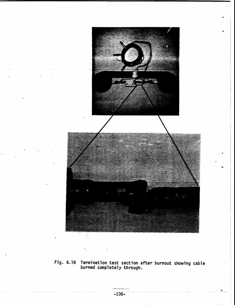
Fig. 6.19 Termination test section after burnout showing cableburned completely through.

-106-

40

conductor failed in the middle of the sheathed section between the tee

block and current bus connection. This should be expected to be the

weakest point in the test section because it is furthest away from low

current density current bus connections and the extra heat capacity of

the helium tee block steel. The implication for a real superconducting

coil is that current burnout would probably occur between tee block and

the beginning of the coil winding, since this section would probably have

the least heat capacity and the highest current density in the coil.

The adiabatic heating curve for copper (Fig. -6.15) was used to

estimate the time to burnout and was found to be within a factor of 2 of

the actual value. The discrepancy can be attributed principally to the

presence of the sheath material and implies that all materials that have

significant heat capacity or current sharing capability, and are in close

contact with the conductor, should be included in the computation. Then

the adiabatic heating curve for copper and/or other materials should be

a relative good predictor of conductor heating behavior.

-107-

6.3 References for Section 6

1. R.J. Thome, et al., "Safety and Protection for Large Scale Supercon-ductivity Magnets - FY83 Report, MIT Plasma Fusion Center Report No.PFC/RR-83-33, December 1983, pp. 111-117.

2. J.R. Miller and J.W. Lue, "Designing Internally Cooled Superconductorsfor use in Large Magnets," Proceedings of the Workshop on Stability ofSuperconductors in Helium I and Helium II, Saclay, France, November16-19, 1981, pp. 247-254, International Institution of Refrigeration,Refrigeration Science and Technology.

3. P. Thullen and J.L. Smith, Jr., "Model for Thermally Sustained Pres-sure Oscillations Associated With Liquid Helium," Advances in Cryo-genic Engineering, Vol. 13, pp. 215-222, Plenum Press, N.Y. 1968.

4. T. Yazaki, A. Tominaga, and Y. Narahara, "Large Heat Transport Due toSpontaneous Gas Oscillation Induced in a Tube With Steep TemperatureGradients," Journal of Heat Transfer, November 1983, Vol. 105, pp.889-894.

-108-

7.0 LABORATORY LIQUID HELIUM DEWAR FAILURE - J.V. Minervini and R.J. Thome

Liquid cryogens are required to maintain superconducting magnets in

the superconducting state so it is not unusual to find large dewars of li-

quid helium and liquid nitrogen located in experimental areas and labora-

tories-where superconducting devices are operated. It is more unusual,

however, to hear reports of significant dewar failures.

On March 19, 1984 the Francis Bitter National Magnet Laboratory ex-

perienced a major dewar failure in one of the laboratory rooms. This

section describes that dewar failure, its probable causes, and some

safety precautions that should always be taken. In addition, a thermo-

dynamic analysis of dewar pressurization is given that provides insight

into the fundamentals of safe dewar operation.

7.1 Dewar Failure

The dewar that failed was a typical, transportable, 25 liter liquid

helium storage dewar. A simplified cross section of the dewar is shown in

Fig. 7.1. The principal components are the spherical helium vessel, the

spherical annular liquid nitrogen shield and an outer spherical vacuum

shell. These components are all suspended from a thin wall neck. They

are fabricated from copper hemispheres and the halves joined by solder at

the equator. An outer stainless steel casing protects the inner vessels

from mechanical damage. The annular gaps between the spherical shells are

evacuated and filled with aluminized mylar superinsulation. The sketch in

Fig. 7.1 shows a helium pressure gauge and pressure relief valve but these

were not present on the dewar that failed. The absence of these safety

Bellows Seal

Nitrogen Vent-

Liquid Helium Filland Discharge

Helium PressureGauge

Helium PressureVacuum Relief Valve

Nitrogen Liquid NitrogenReservoir Fill Line

Vacuum

Helium Inner Helium

Reservoir Assembly

NitrogenOuter ShieldCasing Assembly

Support

Caster-MountedRemovable Dolly

Standard Opening 5/8" O.D. x 0.620" WallLarger Neck Openings Available on Special Order

Fig. 7.1 Simplified cross section of liquid helium dewar.

-110-

devices is not uncommon on many of these dewars. The dewar sits on a frame

with casters so it can be easily rolled around.

The dewar was sitting in a laboratory and exploded during the middle

of a work day. It was totally destroyed and there was significant damage

to the room. The room was unoccupied at the time of the explosion. Figure

7.2 shows a photograph of .the dewar and Fig. 7.3 shows a photograph of the

room after the explosion. The damage to the dewar was complete, with all

of the spherical shells being broken either by failure at the hemispherical

solder joint or by-actual tearing of the metal.

Most of the damage to the room occurred because the dewar separated

into two halves with the top half projected vertically up into the ceiling

and the bottom half driven into the floor. The main projectiles were ver-

tical because the weak- seam was horizontal. Thus, most of the damage was

limited to a cylindrical volume about 8 feet in diameter between the floor

and the ceiling. Most of the room damage derived from the dewar tearing

out a cable tray and flourescent light fixture above with the reaction

force driving the casters into the linoleum floor below.

The probable cause of the failure was an ice blockage in the dewar

neck. The normal method of pressure venting in these dewars is by pres-

sure buildup lifting off a brass plug that sits on top of the fill and

discharge tube. This plug should always be in place except when a trans-

fer tube is inserted for filling or discharging. When the plug is left

out, the ambient temperature air fills the neck tube, condenses on the

cool tube walls and freezes. Eventually, enough air can freeze to com-

pletely block the neck. The steady-state heat leak into the closed helium

-111-

a)

b)

Fig. 7.2 Two(a)(b)-

views of dewar after explosion showingcopper shells and stainless steel outer jacket, andclose-up of inner copper shells and superinsulation.Note the separated solder joint.

-112-

Fig. 7.3 View of dewar and laboratory damage after explosion.The inner copper shells and overhead cable tray arevisible.

-113-

volume drives up the pressure. The next section contains a thermodynamic

ana-lysis of this situation. Without pressure relief, either through a re-

lief valve or burst disk, the pressure will continue to build up, with

possible failure resulting, as happened in this case. The time required

to completely plug up the neck with freezing air can be deceptively short

and is a cumulative process between dewar warm-ups or neck reaming.

Several safety precautions may be taken to prevent such accidents.

These precautions include:

(1) keep neck plug in place except when transferring helium,

(2) maintain liquid nitrogen in shield (suggested interval 3 daysor less),

(3) check for ice blockage in neck of any dewar left unused for 2to 3 days,

(4) ream dewar neck on a regular basis (every day or -so).

These procedures should be followed for all small laboratory dewars

but they are particularly important for dewars that do not have pressure

relief valves or burst disks.

7.2 Thermodynamic Analysis of Pressurized Dewars

If a dewar is unvented, either by design or accident, the thermody-

namic analysis of the pressure rise becomes quite simple. Assume that

the thermodynamic system consists of a mass of helium inside a closed tank

and that the initial state is two-phase helium at a temperature of 4.2 K

and 1 qtmosphere pressure, with a vapor volume fraction of specified value

x. Then any heat energy that leaks into the dewar goes into raising the

internal energy of the helium. The temperature and pressure at any time

after the dewar is sealed is determined by the total amount of energy per

-114-

unit mass input to the system and the initial vapor volume fraction.

This is illustrated in Fig. 7.4 which was generated from the thermo-

dynamic properties of helium. 1 As an illustration, note that a vessel

which is initially full of liquid, x = 0, will experience a relatively

large increase in pressure for a relatively smiall heat input per unit

mass. Hence, it is not desirable to fill a container completely and then

seal it. Of course, the purpose of the dewar is to carry liquid helium,

so it suggests leaving a small amount of ullage, that is, x may be small,

but must be nonzero for safety.

Another simple analysis can be done to determine burst disk dimen-

sions for limiting the maximum pressure in the dewar. A preliminary an-

alysis may be carried out by assuming that during a sudden energy input

the pressure inside the dewar becomes greater than 2.05 times the pressure

outside the vessel. The flow will then be sonic at the point of minimum

area in the vent or burst disk and the flow rate will be determined on

this basis.

The mass flow per unit area under these conditions is:

k+1W k ( 2 ) -- Pok-.. (7.1)A R k +1O

W = mass flow rateA = cross-sectional area of vent passagek = ratio of specific heatsR = gas constantPO = stagnation pressureTo = stagnation temperature

-115-

35 0

2 atm30-

25 - 4 atm

cl)C>

20

z

3 atm

-15 -

- z 7*0K

10 -... 6K

2 atm

5

SATURATIONCURVE

0.1

0 25 50 T5 100

Fig. 7.4 Temperature and pressure in a container filled with enough liquidhelium to reach a given vapor volume fraction, then sealed at 15psia and subjected to a given total heat input per unit mass.

-1-6

We can express W in terms of the gas produced and by an equivalent

number of liters of liquid helium being vaporized. In these terms, the

above formula can be simplified to the following for helium:

_= 30.2 PO(7.2)

W = liters of liquid helium per second which are vaporizedand vented

A = cross-sectional area (in. 2

Po = stagnation pressure (psi)To = stagnation temperature (K)

If a pressure limit of 50 psi is chosen then:

W = 478 A at 10 KW = 87 A at 300 K

This implies that (if the gas temperature is no higher than 10 K) a

1 in. 2 vent will exhaust 478 liters per second of vaporized helium. At

300 K this drops to 87 liters per second. Both rates are adequate from

the standpoint of safety and lower pressures may be had with larger vents.

The helium venting process may also be considered as the removal of

energy from the system at a certain rate as illustrated in Fig. 7.5. The

heat of vaporization of liquid helium is 2580 joules per liter of liquid.

The latter weights 125 grams. The specific heat of helium gas is 2.32

joules/g K so that for the 125 g in a liter of liquid helium, the specific

heat would be 290 joules/liter K.

The rate of energy removal from the system is then:

LQ = W 2580 + 290 (To - 4.2) (7.3)

-117-

SONIC FLOW THROUGH VENT AT ARATE W/A LITERS OF HELIUMVAPORIZED AND VENTED PERSECOND

LIQUIDHELIUM

HEAT ADDITIONdQdt

Fig. 7.5 Model of helium flow through burst disc for a given heat input rate.

-118-

where W is in liters of helium per second. Substitution for W from the

previous equation gives:

1 dQ WATTS P0 (psi)- -- -- = 30.2 - [2580 + 290 (TO(K) - 4.2)] (7.4)A dt in.2

This relationship is shown plotted for 30 and 50 psi dewar pressures

as a function of To in Fig. 7.6. This figure indicates that each square

inch of vent area is capable of venting several hundred kilowatts of heat

generated in the cold area. For a 2 x 106 joule magnet transferring heat

to the helium liquid for 10 seconds, a one square inch vent would be able

to handle the boil off at an internal pressure of 30 - 50 psia.

While the above analysis is only approximate, it does show that rela-

tively small vents can handle large amounts of heat influx into the low

temperature region. Alternately, it can be concluded that overpressures

can be kept to values of a few psi if desired, by using larger vent areas.

7.3 Summary

A small laboratory dewar suffered a catastrophic failure due to ex-

cess pressure buildup after an ice blockage closed off the vent area of

the neck. This was the result of improper dewar usage. Some recommenda-

tions for safe operating procedures were given but these rules should be

transmitted to laboratory personnel and reinforced on a regular basis.

-119-

0

U)

i

00of)

00IT

00I',

?*U!/MX 'V3NV .N3A .LINfl 83d IVAObd38 ±iVH

-120-

00

0

o e

-wuJ

wCL

z0o ~

0z

C0

xOI

4-.

U

-)

-)

C

0 S

'4-34

u

0L

00

00(D

00N

00

00

ai I I

A simple thermodynamic analysis was developed in order to estimate

maximum dewar pressures in a sealed system and burst disk size to gain in-

sight into the fundamental requirements for safe operation. Manufacturers

instructions and code requirements should, however, always be followed.

-121-

8.0 SAFETY RELATED ACTIVITIES - R.J. Thome

8.1- Publications

The following papers were published in FY84 and present work which

was partially supported by the PFC contract monitored by INEL (DOE Con-

tract No. DIE-AC02-78ET51913).

1. R.J. Thome, J.M. Tarrh, R.D. Pillsbury, Jr., W.R. Mann and W.G.Langton, "Protection of Toroidal Field Coils Using Multiple Circuits,"10th Symposiuum on Engineering Problems of Fusion Research, Proceed-ings, IEEE Contract Number 83CH1916-6 NPS, Vol. 2, Philadelphia,Penn., December 1983, pp. 2059-2063.

2. R.J. Thome, R.D. Pillsbury, Jr., W.G. Langton and W.R. Mann, "Magneticto Kinetic Energy Conversion Following Structural Failure," 1984 Ap-plied Superconductivity Conference, to be published in IEEE Trans.Magnetics, MAG-21 (January 1985, Tentatively) San Diego, CA, Septem-ber 1984.

8.2 MESA Subcontract

The MIT Plasma Fusion Center is under subcontract to MESA Corpora-

tion, Ogden, Utah to support their contract "Experience With Magnet Ac-

cidents." The period of performance for the MIT contract is February 1984

through February 1985.

As part of the activity, MIT has prepared a survey which was distri-

buted to the major centers of magnet activity in the U.S. The purpose of

the survey is to gather data on magnet failure experience and classify re-

sults. Results will be'analyzed by MESA Corporation with the help of MIT

and will be presented in a separate report.

-122-

doe/et/51013-137 safety and protection for large

Documents