does postponing minimum retirement age improve …ftp.iza.org/dp9834.pdf · discussion paper series...

Forschungsinstitut zur Zukunft der ArbeitInstitute for the Study of Labor

DI

SC

US

SI

ON

P

AP

ER

S

ER

IE

S

Does Postponing Minimum Retirement Age Improve Healthy Behaviours Before Retirement?Evidence from Middle-Aged Italian Workers

IZA DP No. 9834

March 2016

Marco BertoniGiorgio BrunelloGianluca Mazzarella

Does Postponing Minimum Retirement Age

Improve Healthy Behaviours Before Retirement?

Evidence from Middle-Aged Italian Workers

Marco Bertoni University of Padova

Giorgio Brunello

University of Padova and IZA

Gianluca Mazzarella

University of Padova

Discussion Paper No. 9834 March 2016

IZA

P.O. Box 7240 53072 Bonn

Germany

Phone: +49-228-3894-0 Fax: +49-228-3894-180

E-mail: [email protected]

Any opinions expressed here are those of the author(s) and not those of IZA. Research published in this series may include views on policy, but the institute itself takes no institutional policy positions. The IZA research network is committed to the IZA Guiding Principles of Research Integrity. The Institute for the Study of Labor (IZA) in Bonn is a local and virtual international research center and a place of communication between science, politics and business. IZA is an independent nonprofit organization supported by Deutsche Post Foundation. The center is associated with the University of Bonn and offers a stimulating research environment through its international network, workshops and conferences, data service, project support, research visits and doctoral program. IZA engages in (i) original and internationally competitive research in all fields of labor economics, (ii) development of policy concepts, and (iii) dissemination of research results and concepts to the interested public. IZA Discussion Papers often represent preliminary work and are circulated to encourage discussion. Citation of such a paper should account for its provisional character. A revised version may be available directly from the author.

IZA Discussion Paper No. 9834 March 2016

ABSTRACT

Does Postponing Minimum Retirement Age Improve Healthy Behaviours Before Retirement?

Evidence from Middle-Aged Italian Workers* By increasing the residual working horizon of employed individuals, pension reforms that raise minimum retirement age are likely to affect the returns to investments in health-promoting behaviours before retirement, with consequences for individual health. Using the exogenous variation in minimum retirement age induced by a sequence of Italian pension reforms during the 1990s and 2000s, we show that Italian males aged 40 to 49 reacted to the longer time to retirement by raising regular exercise and by reducing smoking and regular alcohol consumption. Dietary habits were also affected, with positive consequences on obesity and self-reported satisfaction with health. JEL Classification: H55, I12, J26 Keywords: retirement, working horizon, healthy behaviours, pension reforms Corresponding author: Marco Bertoni Department of Economics and Management “Marco Fanno” University of Padova Via del Santo 33 35123 Padova Italy E-mail: [email protected]

* We thank Martina Celidoni, Michele De Nadai, Jan Marcus, Giacomo Pasini, Lorenzo Rocco, Adriana Topo, Elisabetta Trevisan, Guglielmo Weber, Felix Weinhardt, Francesca Zantomio and the audiences at seminars in Berlin, Padova and Venice for comments and suggestions. Marco Bertoni and Giorgio Brunello gratefully acknowledge financial support from the POPA_EHR project at the University of Padova. The usual disclaimer applies.

2

Introduction

There is substantial research in health economics exploring the causal effects of retirement on

individual health and health behaviours. This literature consistently reports that the transition

into retirement has positive short-term effects both on self-reported health and on indices of

physical health. Recent evidence includes Insler, 2014, for the U.S., Coe and Zamarro, 2011,

and Eibich, 2015, for Europe and Zhao et al., 2013, for Japan. Some studies emphasize the

positive changes in health-promoting behaviours – such as additional physical exercise and

reductions in drinking and smoking – when explaining the positive effects of retirement on

overall health (Celidoni and Rebba, 2015, and Kaempfen and Maurer, 2016).1 These positive

effects, however, may be short-lived and disappear with time (the so-called ‘honeymoon

effect’ of retirement).2

The causal impact of retirement on health is typically identified using the exogenous

variation provided by changes in the eligibility conditions for early or full retirement, that

affect retirement patterns without having a direct impact on health (see Coe and Zamarro,

2011). These changes, however, affect not only the individuals who are close to eligibility,

but also younger individuals, and in particular those who – in the absence of constraints –

would choose an optimal retirement age that falls below the minimum required by retirement

rules. Therefore, optimal health behaviours may change even before retirement.

Compared to the growing evidence on the impact of retirement on health, less is known on

the effects of a longer working horizon on individual behaviours before retirement, and what

1 Conversely, Godard, 2016, finds that the retirement transition has a positive effect on the

incidence of obesity among European workers. This effect is particularly pronounced among

those who were employed in blue-collar and physically demanding jobs. The studies on the

effects of retirement on cognition generally find negative effects (see Rohwedder and Willis,

2010, Adams et al., 2012, Mazzonna and Peracchi, 2012, and Celidoni et al., 2013). The

evidence is less clear-cut for mental health (see Charles, 2004, Börsch-Supan and Jürges,

2009, Johnston and Lee, 2009, Clark and Fawaz, 2009, Bonsang and Klein, 2012, Bertoni

and Brunello, 2014, and Fonseca et al., 2015). 2 For instance, Mazzonna and Peracchi, 2014, and Bertoni et al., 2015, estimate that - given

age - a longer time spent in retirement has a negative effect on an index of overall physical

health and on muscle strength, a robust predictor of disability, cardiovascular diseases and

mortality.

3

is known does not include health-promoting behaviours. Hairault et al., 2010, for instance,

shows that French workers exposed to an exogenous increase in their expected retirement age

increase job search effort. They explain this finding by showing that the economic returns to

jobs depend on their expected duration, which increases with retirement age. Following a

similar argument, Montizaan et al., 2010, and Brunello and Comi, 2015, use Dutch and

Italian data and show that policies that increase the residual working horizon have positive

consequences on training participation by active older workers.3 In a study especially close to

ours, De Grip et al., 2012, find that a Dutch reform reducing pension rights and postponing

the minimum retirement age of public sector workers has reduced their mental health.

In this paper, we use data on several cohorts of middle aged Italian working men during the

period 1997 to 2011 to study the impact of changes in minimum retirement age – induced by

reforms affecting eligibility conditions – on health-promoting behaviours before retirement.

By considering only male workers aged 40 to 49, we focus on individuals who are generally

not eligible for retirement and at the same time are not too far from it. Changes in health-

promoting behaviours affect health. Health before retirement is likely to be higher among

middle aged men if better health increases the net utility gains associated to a longer working

horizon. For instance, if earnings and employment in the additional period before retirement

depend on health, affected individuals have an incentive to keep fit so as to reap these

benefits.

Italy provides an interesting setup for the issue at hand, because of the sequence of pension

reforms that occurred during the period under study (see e.g. Angelini et al., 2009). Even

before these reforms, eligibility for early retirement required in most cases that social security

contributions be paid for at least 35 years. The sequence of reforms progressively tightened

eligibility requirements in terms of both age and accrued years of contributions, thereby

3 Montizaan and Vendrik, 2014, find that the same policies negatively affected job

satisfaction of treated Dutch workers. A longer working horizon may also have inter-

generational consequences on the children of potential retirees. Manacorda and Moretti,

2006, find negative effects of a longer parental working horizon (and thus higher parental

income) on the nest-leaving decisions of Italian youngsters. Battistin, et al., 2014, find that

policies raising the retirement age have negatively affected the supply of informal childcare

provided by Italian grandparents, thereby reducing the number of grandchildren.

4

generating exogenous variation in the expected minimum retirement age for comparable

workers observed in different years – when different retirement laws were in place.

We study the effects of changes in minimum retirement age on health-promoting behaviours,

including regular exercise, refraining from smoking and drinking alcohol regularly, and

dietary habits such as refraining from eating red meat or imbibing soft drinks at least once a

day, and eating fruit or vegetables at least once a day. We also consider the effects on the

body mass index.4

Our empirical approach relies on instrumental variables. In Italy, the minimum time to

retirement combines age requirements – that are clearly exogenous – and requirements on the

years of paid social security contributions, that depend on individual careers and are likely to

be endogenous, because negative health shocks affect both health behaviours and working

careers. We instrument minimum actual years to retirement, computed using information on

the actual years of paid contributions, with minimum potential years to retirement – obtained

by replacing the number of years of paid social security contributions with potential

experience – measured as age minus school leaving age, a pre-determined variable in our

setup. Conditional on age-by-school leaving age dummies, sector dummies and non-linear

trends in birth cohort, the only remaining source of variation in the instrument is generated by

the different retirement rules in place in different years – which are exogenous to individual

choices.

We find that a one-year increase in minimum actual years to retirement increases the

likelihood of exercising regularly by 3.28 percentage points (equivalent to 15.74 percent of

the mean value of the outcome in the full sample) and the likelihood of refraining from

smoking and drinking regularly by 3.22 and 2.50 percentage points (equivalent respectively

to 4.88 and 5.40 percent of the mean value of the outcome in the full sample). There is also

evidence that a longer time to retirement reduces the consumption of red meat and soft

drinks, and the prevalence of obesity, although these estimated effects are imprecise. Overall,

self-reported high satisfaction with own health also increases.

We hasten to stress that the range of health behaviours observed in our data does not exhaust

all the important behaviours that may affect health. For instance, we do not have information

on the use of illicit drugs or unsafe sex. Yet our evidence is highly suggestive that postponing

retirement may improve health before retirement.

4 Cawley and Ruhm, 2011, treat obesity as an health behaviour.

5

During the sample period 1997 – 2011, mean years to retirement in our data increased by

about three years. Back-of-the-envelope calculations suggest that the longer minimum

working horizon has had important effects on measured health-promoting behaviours, raising

the frequency of regular exercise by more than 9.8 percentage points – equivalent to more

than 40 percent of the mean value of the outcome in the full sample, a large amount – and

reducing the incidence of smoking and regular drinking by 9.6 and 7.5 percentage points,

equivalent respectively to about 15 and 16 percent of the mean value of the outcomes in the

full sample.

Since these effects are sizeable, especially for physical activity, a natural concern is that the

observed trend in minimum retirement age is capturing the negative trend in several risky

health behaviours, described for instance by Cawley and Ruhm, 2011, for the United States,

and by the OECD, 2015. To dispel this concern, we control for the long-term changes in

behaviours that are not attributable to pension reforms by including in our regressions a

time-varying index of each behaviour for individuals not affected by these reforms (males

aged 65 to 75) or only marginally affected (females aged 40 to 49 who are not in the labour

force or males aged 25 to 30). However, irrespectively of the chosen control group, our

qualitative results are unchanged.

Understanding the effects of a longer working horizon on behaviours before retirement is

important. Several OECD countries have recently introduced pension reforms that raise

minimum retirement age in order to deal with the increased burden of population ageing on

public finances. By delaying retirement and by increasing the residual working horizon of

employed individuals, these reforms may generate unexpected costs and benefits. In this

paper, we highlight that one benefit could be better health before retirement, as constrained

individuals react to the longer horizon by investing in healthy behaviours and reducing

unhealthy ones. Ceteris paribus, in countries with universalistic public health care, better

health before retirement may generate important savings, and these savings should be

accounted for when evaluating the impact of pension reforms.

The paper is organized as follows. In Section 1, we introduce the institutional background

and the sequence of pension reforms affecting minimum retirement age in Italy. Section 2

presents the data. We discuss the empirical setup in Section 3 and results in Section 4.

Conclusions follow.

6

1. Institutional Background: Recent Italian Pension Reforms

To cope with the fiscal consequences of population ageing, starting from the early 1990s

many European countries – including Italy – have undertaken structural changes in their

social security systems, including significant increases in minimum retirement age. In this

paper, we focus on the sequence of Italian social security reforms that took place between

1997 and 2011 – the period covered by our data – and repeatedly changed retirement

eligibility rules.5

Before 1992, the minimum age for old-age pension for men was 60 for employees in the

private sector and for self-employed workers, and 65 for public sector employees -

conditional on having paid social security contributions for at least 15 years. Early retirement

with a seniority pension was instead possible at any age for workers who had paid social

security contributions for at least 35 years.6 The first social security reform (the so-called

“Amato” reform – from the name of the Prime Minister at the time of its implementation)

took place in 1992 and introduced a progressive increase in the requirements for eligibility to

old age pensions, that were expected to reach at least 20 years of paid contributions and age

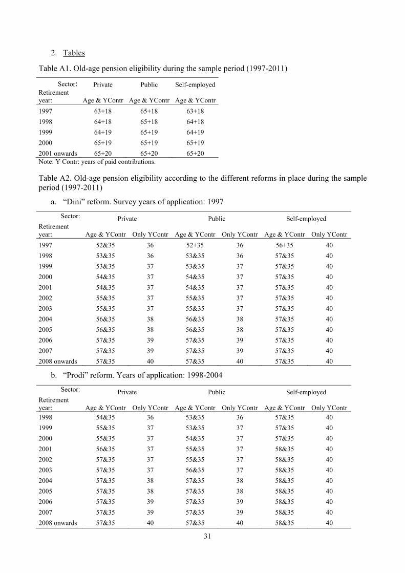
65 by 2001, as shown in Table A1 in the Appendix.

In 1995, a second major reform (the “Dini” reform) tightened the eligibility requirements for

seniority pensions, that were to raise gradually from 1996 to 2008 until either 40 years of

paid contributions independently of age, or 57 years of age and 35 years of paid

contributions.7 The reform also prescribed a faster increase of eligibility requirements for the

self-employed, as documented in Table A2 in the Appendix, where we summarize all

changes in seniority pension eligibility rules introduced by the reforms of interest. After only

5 We exclude the Fornero reform, that substantially changed eligibility rules in 2012. See

Angelini et al., 2009, and Bottazzi et al., 2011, among others for further details on the

pension reforms occurring during our sample period. 6 Since our empirical analysis is restricted to men, we do not discuss here the changes in

pension eligibility rules that apply to females. 7 By introducing eligibility requirements for seniority pensions, this reform abolished the so-

called “baby-pensions”, that since 1973 allowed public employees with at least 20 years of

paid contributions to retire independently of age. This requirement was set as low as 14 years,

6 months and 1 day for married women with children who were employed in the public

sector.

7

three years, in 1998, pension eligibility rules changed again with the “Prodi” reform, that

accelerated the transition period and increased the minimum retirement age to 58 for the self-

employed.

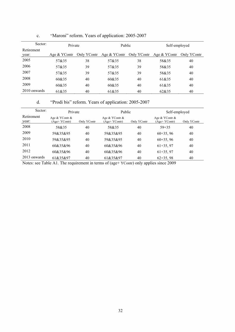
The fourth reform took place in 2005, when Welfare Minister Roberto Maroni changed again

the eligibility requirements for seniority pensions, introducing a sharp 3-year increase in

minimum eligibility age (the so-called “scalone”) from 57 to 60 years for public and private

employees, and from 58 to 61 for the self-employed, starting from year 2008. However, in

2007, the new left-wing government led by Romano Prodi (or “Prodi bis”) postponed the

proposed 3-year increase to 2011, introducing instead a gradual adjustment in the

requirements, starting again from 2008, as documented in Table A2. For this reason, no

worker has actually retired under the requirements prescribed by the “Maroni” reform. Yet,

this reform is still relevant for our purposes, as it changed the expected minimum retirement

age for workers during the years from 2005 to 2008. In addition, under the “Prodi bis”

regime, eligibility to seniority pensions was made conditional to achieving a further

threshold, defined in terms of the sum of age and years of contributions – that also varies by

year of retirement and sector (see Table A2).

This sequence of reforms has generated exogenous variation in the minimum retirement age

of workers with the same age, who have paid social security contributions for the same

number of years and belong to the same sector, but are observed in different years (i.e. were

born in different cohorts), when different retirement laws were in place. To isolate this

variation from endogenous changes in the length of working careers, we define potential

years to retirement PYR at time t as the minimum number of years to retirement prescribed by

the law in place at the time, when the years of paid social security contributions are set equal

to the years of potential labour market experience, or the difference between age and school

leaving age.8 This measure differs from actual years to retirement YR, that are based instead

on actual rather than potential labour market experience.

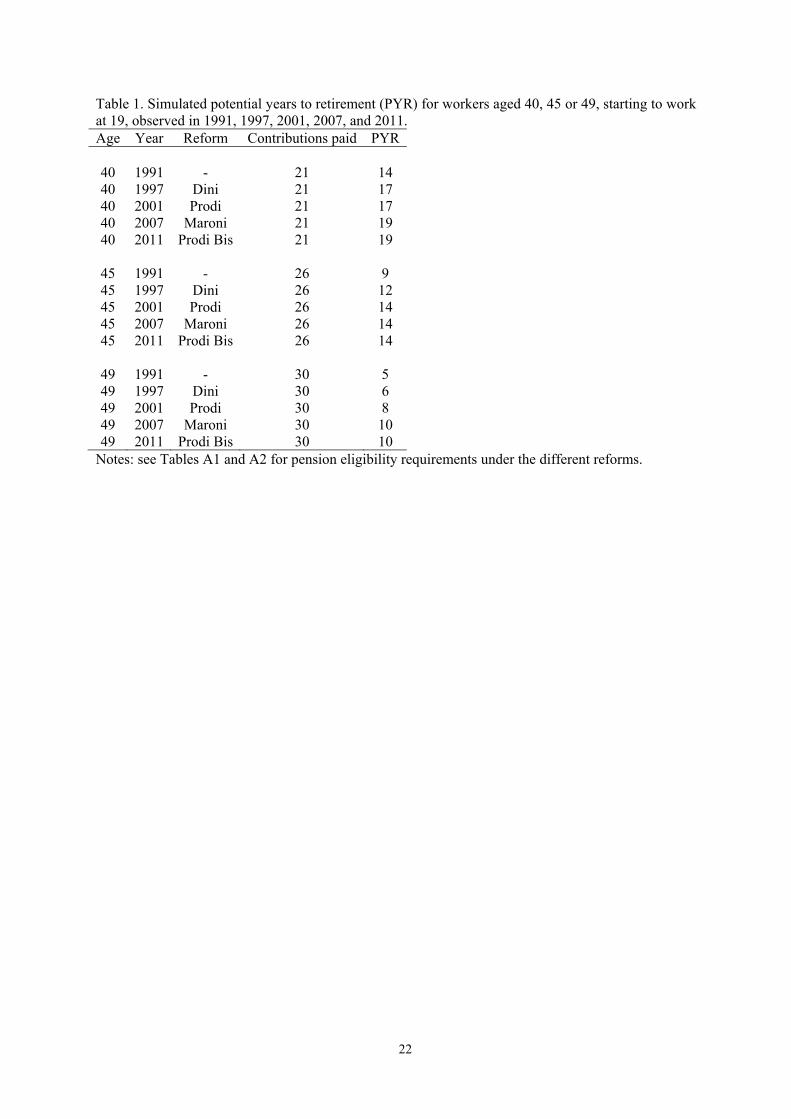
We illustrate how PYR varies over time with the example shown in Table 1, where we

consider hypothetical private sector employees aged 40, 45 and 49 in 1991, 1997, 2001, 2007

and 2011, who started their continuous careers at age 19, after completing secondary school.

8 By so doing, we are assuming that individual labour market careers are continuous. We

compute school leaving age as the canonical number of years required to complete the

highest attained school degree plus six – the school starting age.

8

It turns out that PYR increased from 14 in 1991 to 19 in 2011 for those aged 40, from 9 to 14

years for those aged 45 and from 5 to 10 for those aged 49. Especially for older workers, the

bulk of this increase occurred between 1997 and 2011.

Pension reforms in Italy have also modified pension benefits. The major change occurred in

1995, before the start of our sample period, with the transition from a system based on

defined benefits to a system using defined contributions. Another important change occurred

instead during our sample period, when in 2007 the second Prodi government (“Prodi bis”)

reduced the coefficients used to transform accumulated contributions into pension benefits

for workers retiring from 2010 onwards. Since this change could have altered health

behaviours independently of the changes in minimum retirement age, we account for it in our

empirical analysis.

2. The Data

Our data consist of two samples, a main and an auxiliary sample. The main sample is from

the survey “Aspetti della Vita Quotidiana” (Aspects of Daily Life, hereafter AVQ), carried

out on a yearly basis by the Italian Bureau of Statistics (ISTAT), and the auxiliary sample is

from the Survey on the Income and Wealth of Italian Households (SHIW from now on),

conducted on a bi-annual basis by the Bank of Italy.

AVQ is a cross-sectional annual survey implemented on a sample of about 50,000

individuals. It covers several aspects of daily life, including behaviours such as exercising,

smoking, drinking and dietary habits. We use the waves from 1997 to 2011 (for a total of 14

different years, as in 2004 the survey did not took place), and focus on middle aged (age 40 to

49) males, who are generally too young to be retired but not too far from retirement. We

exclude females because their labour market careers – a crucial aspect of our empirical

exercise – are often more discontinuous than those of men because of childbearing

responsibilities. After eliminating from the sample the very few who are retired, disabled or

have never worked in their life, as well as those with missing values in the variables used in

the analysis we end up with a final sample of 38,966 individuals.

We construct the following indicators of healthy lifestyles: a dummy equal to 1 if the

individual exercises on a regular basis, and 0 otherwise; a dummy equal to 1 if he does not

smoke, and 0 otherwise; a dummy equal to 1 if he does not drink alcohol regularly and 0

9

otherwise;9 a dummy equal to 1 if he refrains from eating red meat at least once a day and 0

otherwise; a dummy equal to 1 if he eats vegetables or fruit at least once a day, and 0

otherwise; a dummy equal to 1 if he refrains from imbibing soft drinks at least once a day,

and 0 otherwise; and a dummy equal to 1 if his BMI is below 30 (not obese), and 0 otherwise.

We also define as indicator of health satisfaction a dummy equal to 1 if the individual is very

satisfied with his own health, and 0 otherwise.

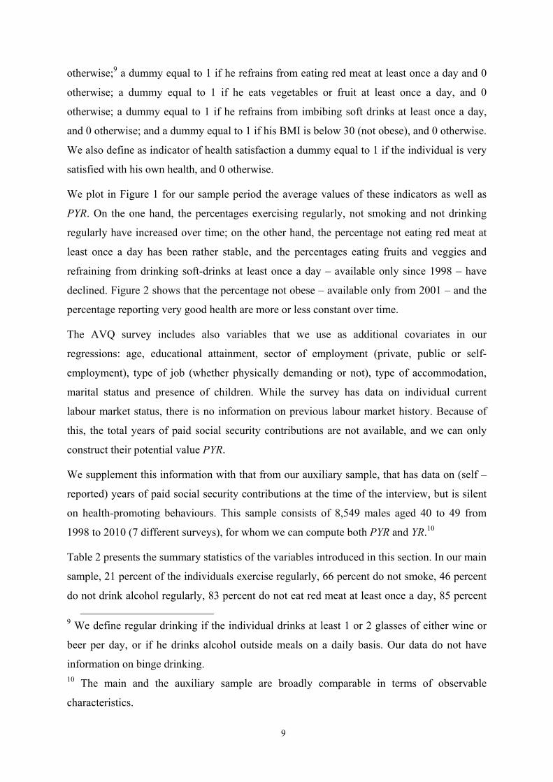
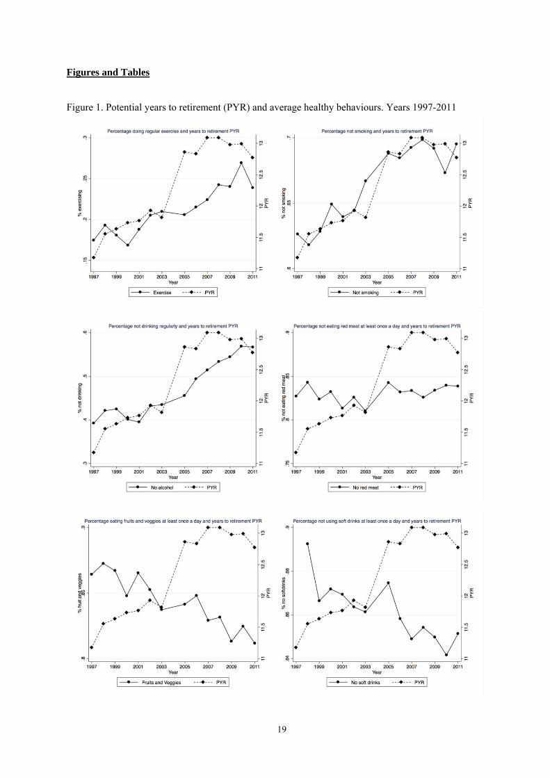
We plot in Figure 1 for our sample period the average values of these indicators as well as

PYR. On the one hand, the percentages exercising regularly, not smoking and not drinking

regularly have increased over time; on the other hand, the percentage not eating red meat at

least once a day has been rather stable, and the percentages eating fruits and veggies and

refraining from drinking soft-drinks at least once a day – available only since 1998 – have

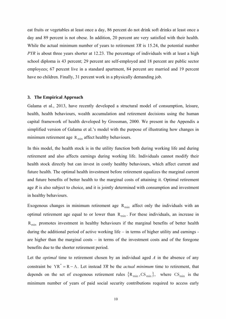
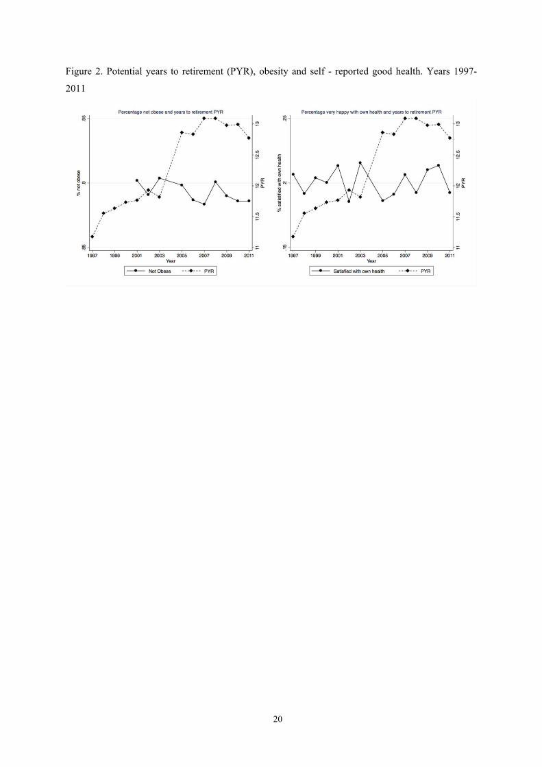
declined. Figure 2 shows that the percentage not obese – available only from 2001 – and the

percentage reporting very good health are more or less constant over time.

The AVQ survey includes also variables that we use as additional covariates in our

regressions: age, educational attainment, sector of employment (private, public or self-

employment), type of job (whether physically demanding or not), type of accommodation,

marital status and presence of children. While the survey has data on individual current

labour market status, there is no information on previous labour market history. Because of

this, the total years of paid social security contributions are not available, and we can only

construct their potential value PYR.

We supplement this information with that from our auxiliary sample, that has data on (self –

reported) years of paid social security contributions at the time of the interview, but is silent

on health-promoting behaviours. This sample consists of 8,549 males aged 40 to 49 from

1998 to 2010 (7 different surveys), for whom we can compute both PYR and YR.10

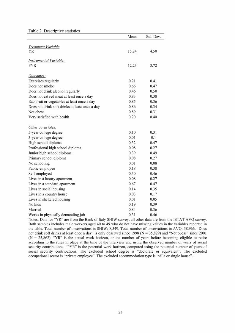
Table 2 presents the summary statistics of the variables introduced in this section. In our main

sample, 21 percent of the individuals exercise regularly, 66 percent do not smoke, 46 percent

do not drink alcohol regularly, 83 percent do not eat red meat at least once a day, 85 percent

9 We define regular drinking if the individual drinks at least 1 or 2 glasses of either wine or

beer per day, or if he drinks alcohol outside meals on a daily basis. Our data do not have

information on binge drinking. 10 The main and the auxiliary sample are broadly comparable in terms of observable

characteristics.

10

eat fruits or vegetables at least once a day, 86 percent do not drink soft drinks at least once a

day and 89 percent is not obese. In addition, 20 percent are very satisfied with their health.

While the actual minimum number of years to retirement YR is 15.24, the potential number

PYR is about three years shorter at 12.23. The percentage of individuals with at least a high

school diploma is 43 percent; 29 percent are self-employed and 18 percent are public sector

employees; 67 percent live in a standard apartment, 84 percent are married and 19 percent

have no children. Finally, 31 percent work in a physically demanding job.

3. The Empirical Approach

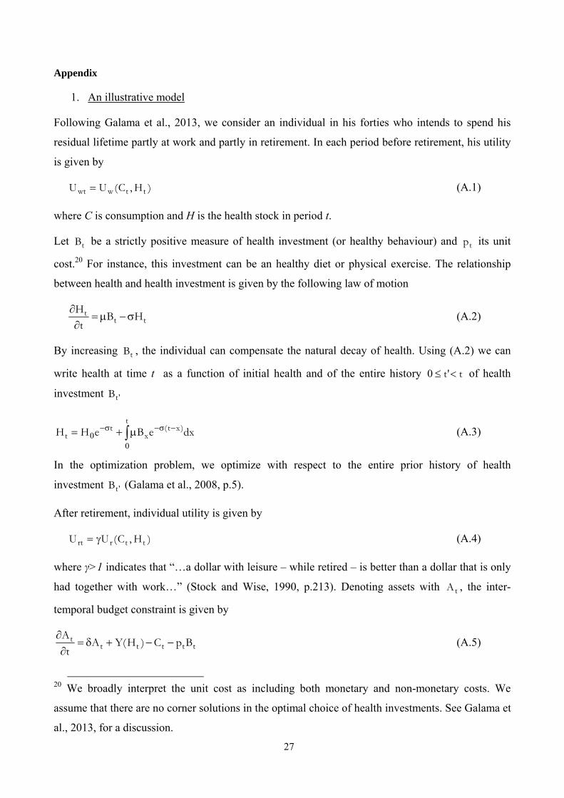
Galama et al., 2013, have recently developed a structural model of consumption, leisure,

health, health behaviours, wealth accumulation and retirement decisions using the human

capital framework of health developed by Grossman, 2000. We present in the Appendix a

simplified version of Galama et al.’s model with the purpose of illustrating how changes in

minimum retirement age minR affect healthy behaviours.

In this model, the health stock is in the utility function both during working life and during

retirement and also affects earnings during working life. Individuals cannot modify their

health stock directly but can invest in costly healthy behaviours, which affect current and

future health. The optimal health investment before retirement equalizes the marginal current

and future benefits of better health to the marginal costs of attaining it. Optimal retirement

age R is also subject to choice, and it is jointly determined with consumption and investment

in healthy behaviours.

Exogenous changes in minimum retirement age minR affect only the individuals with an

optimal retirement age equal to or lower than minR . For these individuals, an increase in

minR promotes investment in healthy behaviours if the marginal benefits of better health

during the additional period of active working life – in terms of higher utility and earnings -

are higher than the marginal costs – in terms of the investment costs and of the foregone

benefits due to the shorter retirement period.

Let the optimal time to retirement chosen by an individual aged A in the absence of any

constraint be ARYR* . Let instead YR be the actual minimum time to retirement, that

depends on the set of exogenous retirement rules minmin CS,R , where minCS is the

minimum number of years of paid social security contributions required to access early

11

retirement, on individual age, and on accumulated social security contributions at age A,

defined as CS.

By modifying minR and minCS , policy makers can alter minimum time to retirement, which

in turn affects the behaviour of individuals for whom YRYR* holds. We model the

empirical relationship between actual minimum years to retirement and healthy behaviours as

follows

itititit XYRB (1)

where the indices i and t are for the individual and time, B is for healthy behaviours, X is a

vector of controls, that includes age by school leaving age dummies, dummies for sector of

employment and a cubic trend in cohort of birth, and ε is the error term. Since our sample

consists of male workers aged 40 to 49 and in Italy transitions from a sector to another are

infrequent in this age range,11 we treat both school leaving age and sector of employment as

pre-determined variables.

The parameter β measures the marginal effect of a one-year increase in the actual minimum

time to retirement on healthy behaviours. Denote with s the share of individuals with

YRYR* and assume that u and c are the marginal effects of YR on B for the sub-groups

with YRYR* and YRYR* , respectively. Then

s

YR

YR

ss

YR

Bc 1 , because

0u . Therefore, the estimated marginal effect of YR in (1) compounds the effect on the

sub-group with YRYR* and the effect on the share of individuals who are constrained by

the minimum retirement age.

As discussed in Section 2, the sequence of pension reforms introduced by Italian

governments during the 1990s and 2000s repeatedly modified both the minimum retirement

11 Using quarterly data from the Italian Labour Force Survey, we estimate the following year-

to-year average transition rates across sectors for workers aged 40 to 49 during the years

2004 to 2011: 1.44 percent from self-employed to private sector employee; 0.23 percent from

self-employed to public sector employee; 0.09 percent from private to public sector

employee; 0.25 percent from private sector employee to self-employed; 0.08 percent from

public to private sector employee and 0.03 percent from public sector employee to self-

employed.

12

age minR and the minimum number of years of paid social security contributions ( minCS )

required to access to retirement with a seniority pension. These changes – that have been

specific to the self-employed and to public and private sector employees – have generated

variability over time in the minimum number of years to retirement among workers of the

same age, who paid social security contributions for the same number of years and belong to

the same sector (i.e. private, public, self-employed).

Since eligibility requires a minimum number of years of paid social security contributions,

YR is shorter for workers with no employment gaps in their careers, even conditional on age,

sector and school leaving age. One reason for observing discontinuous careers is the

experience of negative health shocks – either currently or in the past – which in turn may

depend on the adoption of unhealthy behaviours. These shocks generate reverse causality, as

people who experience bad health – or adopt unhealthy behaviours – also end up having a

longer working horizon. In this case, conditioning on vector X does not suffice in preventing

OLS estimates of β in Eq. (1) from being inconsistent.

We address reverse causality by instrumenting YR with PYR, the potential years to retirement,

or the minimum residual working horizon under the assumption of continuous careers.

Contrarily to YR, the selected instrument does not depend on individual careers and varies

with age, retirement eligibility conditions and education, that are either exogenous or

predetermined for the relevant age group (40 to 49). Conditional on the variables in vector X,

the residual variation in PYR is due exclusively to the changes in retirement rules that took

place over the years – which we treat as exogenous to individual behaviour.

In the reduced form equation,

RititRitRRit XPYRB (2)

the identification of parameter R as the intention to treat effect of PYR on B requires that,

conditional on vector X, PYR is as good as randomly assigned. In support to this assumption,

we show that - as one would expect if PYR can be treated as random given X - the estimates

of R in (2) are broadly unaffected by the inclusion of an additional set of pre-determined

covariates that are likely to correlate with B - including dummies for region of residence, type

of accommodation (a proxy for wealth), marital status, the presence of kids and working in

physically demanding jobs. The estimated value of R is also largely unaffected when we

add time-varying macroeconomic factors (GDP per capita and the relative prices of each

13

outcome of interest), that are likely to influence the adoption of healthy behaviours and to

correlate with changes in eligibility requirements.

In a similar fashion, if healthy behaviours exhibit a long-term positive trend and this trend is

not included in (2), a positive correlation between B and PYR may simply reflect the omitted

trend rather than the effect of pension reforms. To avoid this, we estimate a specification of

(2) that includes as an additional control the variable gtB , defined as the average regional

value of B for three alterative groups (g): a) males aged 65 to 75, who are not affected by

pension reforms; b) females out of the labour force and aged 40 to 49, who are also unlikely

to be affected; c) young males aged 25 to 30, who are far enough from retirement to disregard

changes in PYR in their current behaviours. As reported below, we find that – independently

of the selected control group – the estimates of R are only marginally affected.

The identification of parameter β in Eq. (1) as the (Local) Average Treatment Effect of YR on

B requires two additional conditions: first, we need a significant first-stage relationship

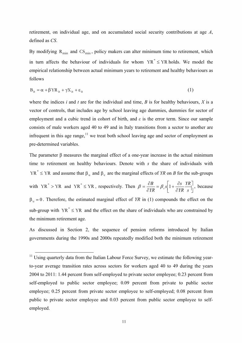
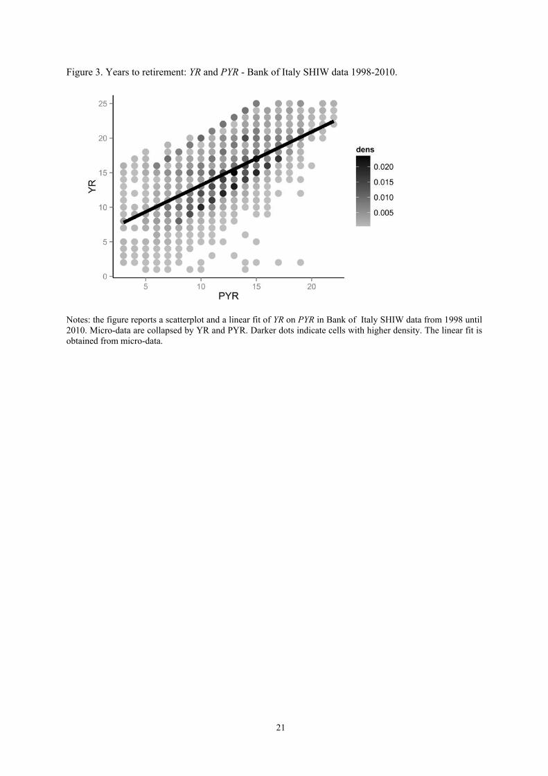
between YR and the selected instrument PYR. Visual evidence that such relationship exists is

reported in Figure 3, where we plot the distribution of YR and PYR in our auxiliary sample, as

well as the linear regression fit, showing a strongly positive association between the two.

Formal evidence is discussed in the next section. Second, we require that PYR influences B

only via its effect on YR, a tenable exclusion restriction in this context.12

As described in the previous section, our key data source - the ISTAT AVQ survey - has

detailed information on the adoption of healthy behaviours, but no information on the years

of paid social security contributions. Since we cannot compute YR using these data, we can

only estimate the reduced form equation (2). We estimate parameter β in Eq. (1) using our

auxiliary SHIW sample and Two-Sample Instrumental Variables (TSIV) (see Angrist and

Krueger, 1992 and Inoue and Solon, 2010).13 Letting π be the effect of PYR on YR in the first

12 We also require a monotonicity condition (see Imbens and Angrist, 1994), stating that

exposure to longer YR cannot lead to shorter PYR. 13 We estimate the first stage using data for 1998, 2000, 2002, 2004, 2006, 2008 and 2010.

Even if we observe in this dataset the accrued years of social security contributions, we still

need to assume continuous careers from the time of observation until retirement (see Battistin

et al., 2009).

14

stage regression, our IV estimate of parameter β is obtained as the ratio

R .14 In all

regressions, we cluster standard errors by cohort, sector and school leaving age.

We estimate equations (1) and (2) for each behaviour separately. However, since the error

terms associated to the different behaviours can be correlated, we also jointly estimate the

system of reduced form equations using seemingly unrelated regressions, but find no

significant change in the standard errors. We also test whether the coefficients associated to

PYR in the reduced form equations are jointly equal to zero, and strongly reject this

hypothesis (p-value<0.01).

4. Empirical Results

If pension reforms that raise minimum retirement age affect at least part of the relevant

population, and workers understand the effects of these changes, average expected retirement

age should raise as YR increases. To document that this is the case, we use our auxiliary

sample drawn from SHIW – where individuals are asked about their expected retirement age

– and regress expected retirement age on minimum age and on the vector of controls X. We

estimate that a one year increase in minimum retirement age raises expected age by about

half a year (0.54, standard error 0.02).15

We estimate equation (2) using a linear probability model and report in Table 3 the estimated

effects of potential minimum time to retirement PYR on healthy behaviours. The table reports

both the estimated coefficients (multiplied by 100) and the percentage effects computed with

respect to the mean of the outcome variable. Panel 1 is for the most parsimonious

specification, that only includes vector X; panel 2 includes additional individual controls;

panel 3 further includes the real GDP per capita, the relevant relative price – measured as the

price of the outcome relative to the average price - and gtB , the regional value of B for males

aged 65 to 75, who are not affected by changes in PYR; panels 4 and 5 are similar to panel 3

14 Inference is carried out by bootstrapping. Notice that, since there is a single endogenous

variable and the model is just identified, our estimation procedure is equivalent to a Two-

Sample Two-Stage Least Squares procedure, which involves computing the fitted values of

YR in the ISTAT AVQ data using the first-stage coefficients estimated in SHIW. 15 See Bottazzi et al., 2006, for additional evidence.

15

except that we use the regional trends in the relevant outcome for males aged 25 to 30 and for

females aged 40 to 49 who are out of the labour force.

Focusing on Panel 1, we find that increasing the residual (potential) working horizon PYR

significantly improves several healthy behaviours. We estimate that a 1-year increase in PYR

raises the probability of practicing sports regularly by 5.92 percent and reduces the

probability of smoking and drinking alcohol on a regular basis by 1.83 and 2.03 percent

respectively. These are statistically significant effects. In addition, increasing PYR by one

year affects nutrition habits by reducing the likelihood of eating read meat and consuming

soft drinks at least once a day by 0.69 and 0.78 percent respectively – although the former

effect is statistically significant only at the 10 percent level. We also detect a small but

imprecisely estimated positive effect of higher PYR on the consumption of fruits and

vegetables. Consistently with these dietary improvements, there is also evidence that a higher

value of PYR increase the probability of not being obese, albeit this effect is imprecisely

estimated.16 Finally, we find that a longer time to retirement improves the probability of

being very satisfied with own health.

Reassuringly for our identification strategy, introducing additional covariates to vector X –

see Panel 2 - does not change our results. Similarly, we do not detect stark changes in our

findings even when we also add macroeconomic controls and regional trends in the outcome

variable for males who are unaffected by the reforms, males very far from retirement age or

females aged 40 to 49 who are out of the labour force – see Panels 3 to 5. Because of this, we

will focus hereafter on the most parsimonious specification in Panel 1.

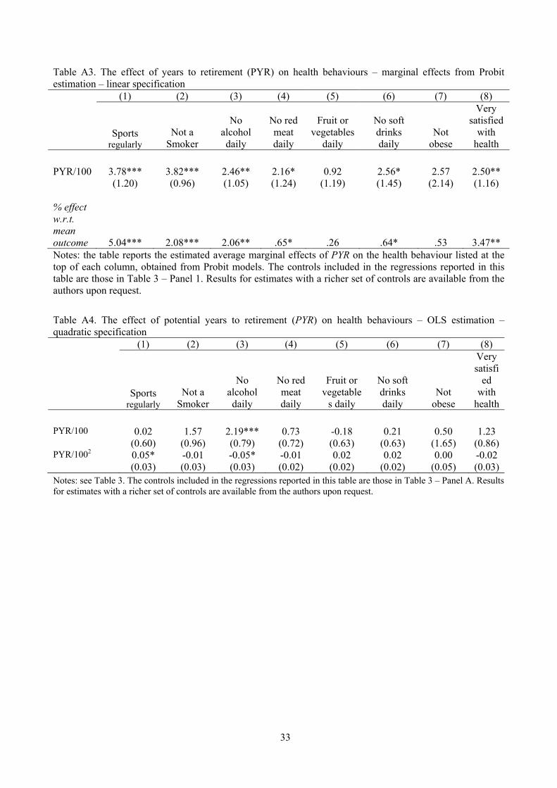
Our empirical findings are robust to several changes in specification. First, Table A3 in the

Appendix shows that results are similar when we compute the marginal effects of PYR on

behaviours using a Probit specification instead of a linear probability model. Second, we

verify whether the linear relationship between behaviours B and PYR - adopted in Eq. (2) - is

overly restrictive by adding to our baseline specification a quadratic term in PYR. As reported

in Table A4 in the Appendix, this term is never statistically significant at the conventional

five percent level of confidence, which lends support to the baseline versus the quadratic

16 This effect is statistically significant at the ten percent level of confidence in less

parsimonious specifications.

16

specification.17 Next, we re-define our outcomes as ordinal variables, but out qualitative

results are still unchanged. For instance, in the case of exercising we distinguish between no

exercising, light physical activity, irregular and regular exercising, and find that an additional

year to retirement has a negative and positive effect of similar size on the former two and

latter two categories respectively.

Last but not least, we consider the potential confounding effects on our estimates of changes

in pension replacement rates, that could have modified healthy behaviours independently of

changes in PYR. The relevant change during our sample period is the method of computation

of pension benefits, that was altered starting in 2007 for those who could retire from 2010

onwards. To control for this effect, we add a dummy equal to 1 for individuals observed in

years 2007-2011 and eligible to retire since 2010, but find no change in our results.18

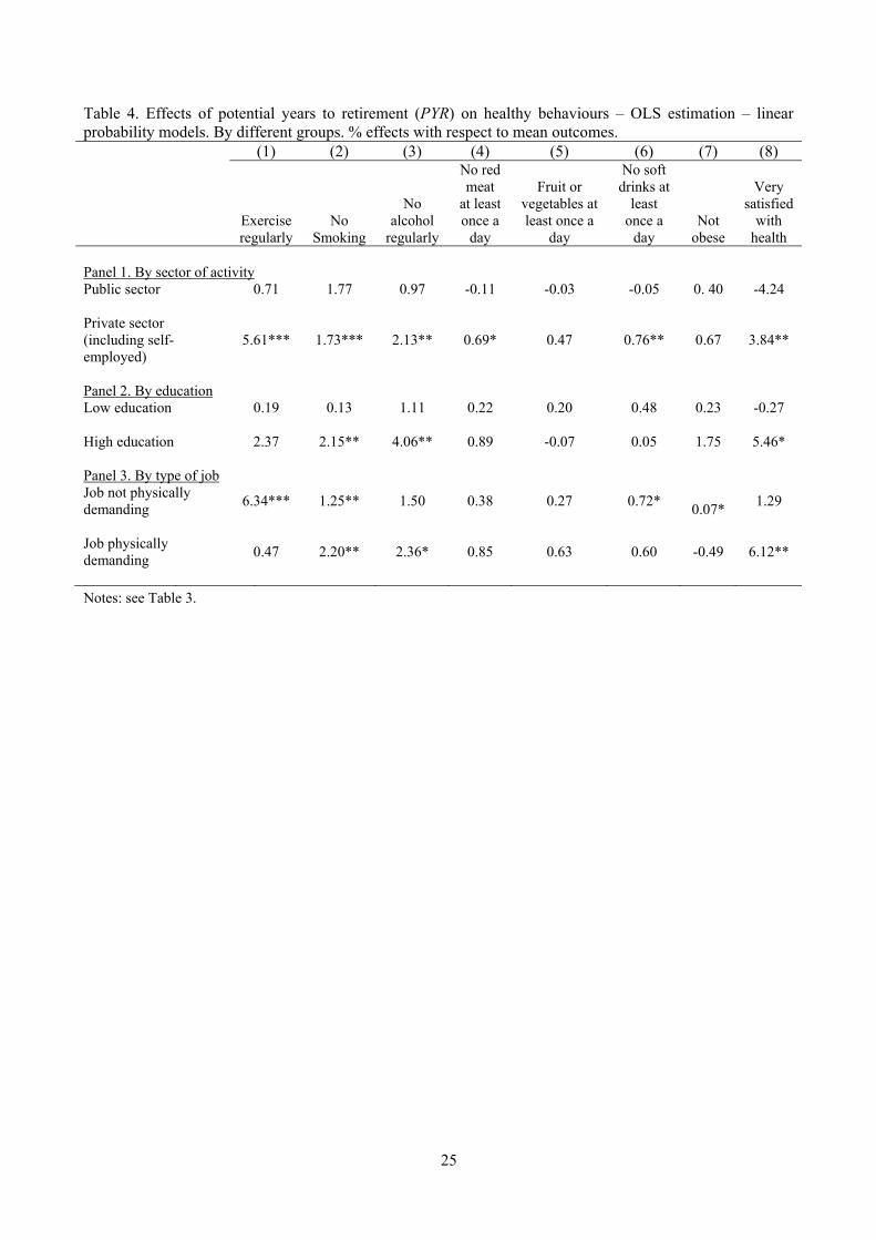
To investigate whether responses to changes in YR are heterogeneous, we estimate separate

regressions by sector of activity (private employees, public employees, self-employed

workers), level of education (below or above high school) and type of job (physically and not

physically demanding job), and report results in Table 4. We find that changes in minimum

retirement age have virtually no effect on public sector workers and generally stronger effects

among the better educated. On the one hand, the better educated may respond more to

changes in minimum retirement age because they typically are more forward looking and

more likely to incorporate future expected changes into their current behaviour. On the other

hand, public employees in Italy have stronger job guarantees than private sector workers, and

therefore may be less concerned with preserving their health in order to work longer. As

expected, we also find that a longer time to retirement does not alter the likelihood of

carrying out regular physical activity by those who are already engaged in a physically

demanding job.19

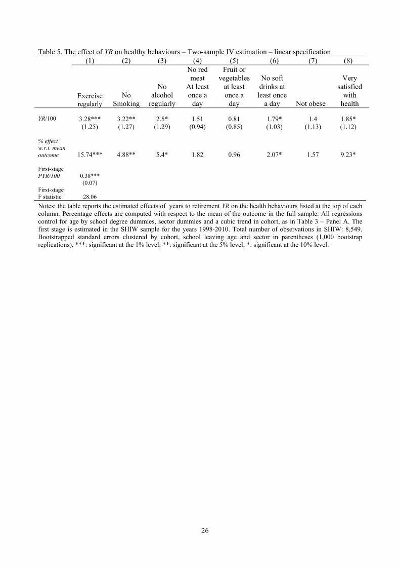
We have presented so far the intention to treat effects of higher potential minimum time to

retirement on healthy behaviours. We now turn to estimating the effects of the actual

minimum time to retirement YR on these behaviours, using potential time PYR as the

17 A specification with dummies for each level of PYR also lends support to the linearity

assumption. 18 The results are available from the authors upon request. 19 Since we find that regular working hours are unaffected by changes in PYR, we conclude

that additional regular exercise occurs mainly during leisure time.

17

instrument for actual time and Two-Sample Instrumental Variables. First, we regress actual

time on potential time and the vector of control X in our auxiliary SHIW sample, and report

the result at the bottom of Table 5. According to our estimates, a 1-year increase in PYR

increases YR conditional on X by 0.38 years. Since the value of the first-stage F statistic for

instrument weakness is 28.06, well above the threshold of 10, our instrument is not weak.

Second, we compute for each behaviour the Two-Sample IV estimate of β as R , and show

our results in the first row of the table (multiplied by 100). We estimate that the IV effects of

YR on B are about 2.5 times larger than the ITT estimates shown in Table 3. When evaluated

at mean values, a one-year increase in the actual minimum time to retirement increases the

likelihood of exercising regularly by 15.74 percent and reduces smoking and drinking by 4.88

and 5.4 percent. We also confirm that higher time to retirement induces a reduction in the

consumption of red meat and soft drinks and in obesity, although these estimates are often

imprecise. Finally, health satisfaction increase by 9.23 percent (statistically significant at the

10 percent level).

These are sizeable effects, especially for physical activity. Back-of-the-envelope calculations

show that, during the sample period 1997 – 2011, mean years to retirement in the SHIW

sample increased from 17 to 20 for those aged 40 and from 8 to 11 for those aged 49. Our

estimates based on the linear specification and the Two-Sample IV method indicate that these

changes have had important effects on healthy behaviours, raising the average probability of

regular exercising from 0.21 to 0.30 (+45%), of not smoking from 0.66 to 0.77 (+16%) and of

not drinking regularly from 0.46 to 0.52 (+13%).

Conclusions

We have investigated the effects of postponing minimum retirement age on healthy

behaviours before retirement using data on several cohorts of middle aged Italian working

men during the period 1997 to 2011, when repeated pension reforms took place in an effort to

contain public expenditure. Because these reforms generated exogenous variation in

minimum retirement age, Italy is an interesting laboratory to study the issue at hand.

While much research has been devoted to establishing whether and how retirement affects the

health of retired individuals, less has been done to understand whether policy measures that

alter the length of the residual working horizon can affect health and healthy behaviours even

18

before retirement. We have estimated the causal effect of changes in the potential as well as

actual minimum number of years to retirement on the health lifestyles of Italian workers aged

40 to 49, who can be 8 to 20 years away from minimum retirement age, and found that -

when evaluated at the mean value of each outcome - a one-year increase in minimum actual

years to retirement raises the likelihood of exercising regularly by 15.74 percent and reduces

smoking and regular drinking by 4.88 and 5.4 percent. Furthermore, a longer time to

retirement increases the probability that red meat and soft drinks are consumed less, and that

fruit and vegetables are consumed more frequently. Because of the improvement in dietary

habits, there is also some evidence that obesity declines. Consistently with these findings, we

also estimate a positive effect on self-reported high satisfaction with health.

Pension reforms that raise minimum retirement age have been introduced in several OECD

countries to deal with the increased burden of population ageing on public finances. By

delaying retirement and by increasing the residual working horizon of employed individuals,

these reforms may reap unexpected dividends. We have highlight that one such dividend

could be better health before retirement, as constrained individuals react to the longer horizon

by investing in healthy behaviours and reducing unhealthy ones. Better health before

retirement may generate important savings to private and public expenditure, and these

savings should be accounted for when evaluating the overall impact of pension reforms.

19

Figures and Tables

Figure 1. Potential years to retirement (PYR) and average healthy behaviours. Years 1997-2011

20

Figure 2. Potential years to retirement (PYR), obesity and self - reported good health. Years 1997-

2011

21

Figure 3. Years to retirement: YR and PYR - Bank of Italy SHIW data 1998-2010.

Notes: the figure reports a scatterplot and a linear fit of YR on PYR in Bank of Italy SHIW data from 1998 until 2010. Micro-data are collapsed by YR and PYR. Darker dots indicate cells with higher density. The linear fit is obtained from micro-data.

22

Table 1. Simulated potential years to retirement (PYR) for workers aged 40, 45 or 49, starting to work at 19, observed in 1991, 1997, 2001, 2007, and 2011.

Notes: see Tables A1 and A2 for pension eligibility requirements under the different reforms.

Age Year Reform Contributions paid PYR

40 1991 - 21 14 40 1997 Dini 21 17 40 2001 Prodi 21 17 40 2007 Maroni 21 19 40 2011 Prodi Bis 21 19



23

Table 2. Descriptive statistics Mean Std. Dev.

Treatment Variable YR Instrumental Variable:

15.24

4.50

PYR 12.23 3.72 Outcomes: Exercises regularly 0.21 0.41 Does not smoke 0.66 0.47 Does not drink alcohol regularly 0.46 0.50 Does not eat red meat at least once a day 0.83 0.38 Eats fruit or vegetables at least once a day 0.85 0.36 Does not drink soft drinks at least once a day 0.86 0.34 Not obese 0.89 0.31 Very satisfied with health 0.20 0.40 Other covariates: 5-year college degree 0.10 0.31 3-year college degree 0.01 0.1 High school diploma 0.32 0.47 Professional high school diploma 0.08 0.27 Junior high school diploma 0.39 0.49 Primary school diploma 0.08 0.27 No schooling 0.01 0.08 Public employee 0.18 0.38 Self-employed 0.30 0.46 Lives in a luxury apartment 0.08 0.27 Lives in a standard apartment 0.67 0.47 Lives in social housing 0.14 0.35 Lives in a country house 0.03 0.17 Lives in sheltered housing 0.01 0.05 No kids 0.19 0.39 Married 0.84 0.36 Works in physically demanding job 0.31 0.46 Notes: Data for “YR” are from the Bank of Italy SHIW survey, all other data are from the ISTAT AVQ survey. Both samples includes male workers aged 40 to 49 who do not have missing values in the variables reported in the table. Total number of observations in SHIW: 8,549. Total number of observations in AVQ: 38,966. “Does not drink soft drinks at least once a day” is only observed since 1998 (N = 35,829) and “Not obese” since 2001 (N = 25,862). “YR” is the actual work horizon, or the number of years before becoming eligible to retire according to the rules in place at the time of the interview and using the observed number of years of social security contributions. “PYR” is the potential work horizon, computed using the potential number of years of social security contributions. The excluded school degree is “doctorate or equivalent”. The excluded occupational sector is “private employee”. The excluded accommodation type is “villa or single house”.

24

Table 3. The effect of potential years to retirement (PYR) on healthy behaviours – OLS estimation – linear probability models. (1) (2) (3) (4) (5) (6) (7) (8)

Exercise regularly

No Smoking

No alcohol

regularly

No red meat

at least once a

day

Fruit or vegetables

at least once a day

No soft drinks at least once a

day Not obese

Very satisfied

with health

Panel 1: includes age by school degree dummies, sector dummies and a cubic trend in cohort

PYR/100 1.23*** 1.21*** 0.94** 0.57* 0.31 0.67** 0.53 0.70** (0.34) (0.34) (0.40) (0.31) (0.27) (0.30) (0.35) (0.33) % effect w.r.t. mean outcome

5.92*** 1.83*** 2.03** 0.69* 0.36 0.78** 0.59 3.47**

Panel 2: includes as additional covariates regional dummies, type of accommodation dummies, having kids, being married and working in physically demanding jobs

PYR/100 1.22*** 1.16*** 0.86** 0.53* 0.29 0.63** 0.57 0.72** (0.33) (0.34) (0.40) (0.30) (0.27) (0.30) (0.35) (0.32) % effect w.r.t. mean outcome

5.86*** 1.76*** 1.86** 0.63* 0.34 0.73** 0.64 3.57**

Panel 3: includes as additional covariates with respect to Panel 2 the real GDP per capita, relative prices and regional trends in the relevant outcome for males aged 65-75

PYR/100 1.21*** 1.10*** 0.84** 0.53* 0.21 0.63** 0.68* 0.72** (0.33) (0.35) (0.40) (0.30) (0.28) (0.30) (0.35) (0.32) % effect w.r.t. mean outcome

5.79*** 1.67*** 1.81** 0.63* 0.25 0.73** 0.76* 3.58**

Panel 4: as Panel 3 but with regional trends in the relevant outcome for males aged 25-30


5.88*** 1.67*** 1.8** 0.64* 0.27 0.70** 0.75* 3.8**

Panel 5: as Panel 4 but with regional trends in the outcome for females not in the labour force aged 40 to 49.


5.86*** 1.67*** 1.89** 0.64* 0.18 0.71** 0.75* 3.67**

Notes: the table reports the estimated effects of PYR/100 on the health behaviour listed at the top of each column. Percentage effects are computed with respect to the mean value of the outcome in the full sample. Total number of observations: 38,966; for “No soft drinks at least once a day”: 35,829; for “Not Obese”: 25,862. In Panel C, we include the relative price of recreational activities in the equation for exercising, tobacco in the equation for smoking, alcohol in the equation for alcohol, meat in the equation for red meat, fruit and vegetables in the equation for fruit and vegetables, soft drinks in the equation for soft drink, and overall food and recreational activities in the equation for obesity. All price data come from the Italian National Statistical Office. Standard errors clustered by cohort, school leaving age and sector in parentheses. ***: significant at the 1% level; **: significant at the 5% level; *: significant at the 10% level.

25

Table 4. Effects of potential years to retirement (PYR) on healthy behaviours – OLS estimation – linear probability models. By different groups. % effects with respect to mean outcomes. (1) (2) (3) (4) (5) (6) (7) (8)

Exercise regularly

No Smoking

No alcohol

regularly

No red meat

at least once a

day

Fruit or vegetables at least once a

day

No soft drinks at

least once a

day Not

obese

Very satisfied

with health

Panel 1. By sector of activity Public sector 0.71 1.77 0.97 -0.11 -0.03 -0.05 0. 40 -4.24 Private sector (including self-employed)

5.61*** 1.73*** 2.13** 0.69* 0.47 0.76**

0.67 3.84**

Panel 2. By education Low education 0.19 0.13 1.11 0.22 0.20 0.48 0.23 -0.27 High education 2.37 2.15** 4.06** 0.89 -0.07 0.05 1.75 5.46* Panel 3. By type of job Job not physically demanding

6.34*** 1.25** 1.50 0.38 0.27 0.72*

0.07* 1.29

Job physically demanding

0.47 2.20** 2.36* 0.85 0.63 0.60 -0.49 6.12**

Notes: see Table 3.

26

Table 5. The effect of YR on healthy behaviours – Two-sample IV estimation – linear specification (1) (2) (3) (4) (5) (6) (7) (8)

Exercise regularly

No Smoking

No alcohol

regularly

No red meat

At least once a

day

Fruit or vegetables

at least once a

day

No soft drinks at least once

a day Not obese

Very satisfied

with health

YR/100 3.28*** 3.22** 2.5* 1.51 0.81 1.79* 1.4 1.85* (1.25) (1.27) (1.29) (0.94) (0.85) (1.03) (1.13) (1.12) % effect w.r.t. mean outcome 15.74*** 4.88** 5.4* 1.82 0.96 2.07* 1.57 9.23* First-stage PYR/100 0.38***

(0.07) First-stage F statistic 28.06

Notes: the table reports the estimated effects of years to retirement YR on the health behaviours listed at the top of each column. Percentage effects are computed with respect to the mean of the outcome in the full sample. All regressions control for age by school degree dummies, sector dummies and a cubic trend in cohort, as in Table 3 – Panel A. The first stage is estimated in the SHIW sample for the years 1998-2010. Total number of observations in SHIW: 8,549. Bootstrapped standard errors clustered by cohort, school leaving age and sector in parentheses (1,000 bootstrap replications). ***: significant at the 1% level; **: significant at the 5% level; *: significant at the 10% level.

27

Appendix

1. An illustrative model

Following Galama et al., 2013, we consider an individual in his forties who intends to spend his

residual lifetime partly at work and partly in retirement. In each period before retirement, his utility

is given by

)H,C(UU ttwwt (A.1)

where C is consumption and H is the health stock in period t.

Let tB be a strictly positive measure of health investment (or healthy behaviour) and tp its unit

cost.20 For instance, this investment can be an healthy diet or physical exercise. The relationship

between health and health investment is given by the following law of motion

ttt HB

t

H

(A.2)

By increasing tB , the individual can compensate the natural decay of health. Using (A.2) we can

write health at time t as a function of initial health and of the entire history t't 0 of health

investment 'tB

dxeBeHH )xt(t

xt

t

00 (A.3)

In the optimization problem, we optimize with respect to the entire prior history of health

investment 'tB (Galama et al., 2008, p.5).

After retirement, individual utility is given by

)H,C(UU ttrrt (A.4)

where γ>1 indicates that “…a dollar with leisure – while retired – is better than a dollar that is only

had together with work…” (Stock and Wise, 1990, p.213). Denoting assets with tA , the inter-

temporal budget constraint is given by

tttttt BpC)H(YA

t

A

(A.5)

20 We broadly interpret the unit cost as including both monetary and non-monetary costs. We

assume that there are no corner solutions in the optimal choice of health investments. See Galama et

al., 2013, for a discussion.

28

where income Y is equal to yearly earnings )H(W t before retirement and to Γ (pension benefits)

after retirement. )H(W t is an increasing and concave function of H, the health stock. Better health

affects earnings both by raising productivity and by increasing the probability of being gainfully

employed, but – as in Galama et al., 2013 – in the model we do not distinguish further between

these two channels.

Changes in minimum retirement age minR affect individual choice only if minR is binding, that is,

if optimal retirement age is lower than or equal to minR . We shall focus on this case. The individual

chooses consumption and healthy behaviours to maximize the following inter-temporal utility

dte)]H,C(U[dte)]H,C(U[Max rtttrt

T

Rrt

ttwtR

s min

min (A.6)

subject to (A.3) and (A.5), where T denotes total lifetime, that we assume to be independent of

health, as in Galama et al., 2013, s is initial age and r is the interest rate. Following Galama et al.,

2008, this is equivalent to maximizing

T

s

tttttt

rtttrt

T

Rrt

ttwtR

sdte]BpC)H(YA[dte)]H,C(U[dte)]H,C(U[Max

min

min

0 (A.7)

where tt e 0 is the co-state variable associated to (A.5). The first order necessary condition for

optimal 'tB when minR't is

T

'tt't

t

't

t

t

tt

rt

't

t

t

rtT

Rrt

't

t

t

wtR

't)p,Z,B(dte]

B

H

H

)H(Yp[dte]

B

H

H

U[dte]

B

H

H

U[

min

min 00 (A.8)

For consumption, the first order condition is

)C,B(eC

U't't

't)r(

't

'wt 00 (A.9)

At the optimum, health investment when minR't equalizes the marginal benefits during both

active working life dte]B

H

H

U[ rt

't

t

t

wtR

'tmin

and after retirement dte]B

H

H

U[ rt

't

t

t

rtT

Rmin

and the net

marginal costs

T

't

t

't

t

t

tt dte]

B

H

H

)H(Yp[0 .

Since the contribution of health to wages ends with retirement, we can re-write (A.8) as follows

29

min

min

R

't

t

't

t

t

trt

't

t

t

wtR

'tdte]

B

H

H

)H(Ydte]

B

H

H

U[ 0

T

'ttmin't't

tt

rt

't

t

t

rtT

R)p,R,C,B(dtepdte]

BH

HU

[min

00

Totally differentiating (A.8) and (A.9) with respect to minR , 'tB and 'tC , we obtain

0

0

21

321

't't

min't't

dCdB

dRdCdB

where Zi

and Z includes minR , 'tB and 'tC .

By Cramer’s rule, we get that

32

min

't

RB

where 1221 >0 because of the second order conditions. Since 2 is negative, the sign of

min

't

RB

depends on the sign of 3 and is positive if

003

min

min

min

min

min

min

R

rRR)r(

R

R

R

wR

H

Ue

H

)H(Y

H

U

In words, postponing minimum retirement age increases optimal healthy behaviours before

retirement if the benefits of a longer working life induced by better health are higher than costs in

terms of leisure due to a shorter retirement period.

For the individuals who are not bound by minimum retirement age, optimal age R can be

determined by inserting the optimal values of tC , tH and tB into the indirect utility function V(R)

and differentiating this function with respect to R. Galama et al., 2013, solve numerically for

optimal retirement age R.

When 0

min

't

R

B, the individual increases her healthy behaviours before retirement, and by so

doing increases her health stock. After retirement, when minR't , he maximizes

T

s

tttttt

rtttrt

T

'tdte]BpCA[dte)]H,C(U[Max 0 (A.9)

The first order necessary condition for optimal 'tB is

30

T

't

tt

rt

't

t

t

rtT

'tdtepdte]

B

H

H

U[ 00 (A.10)

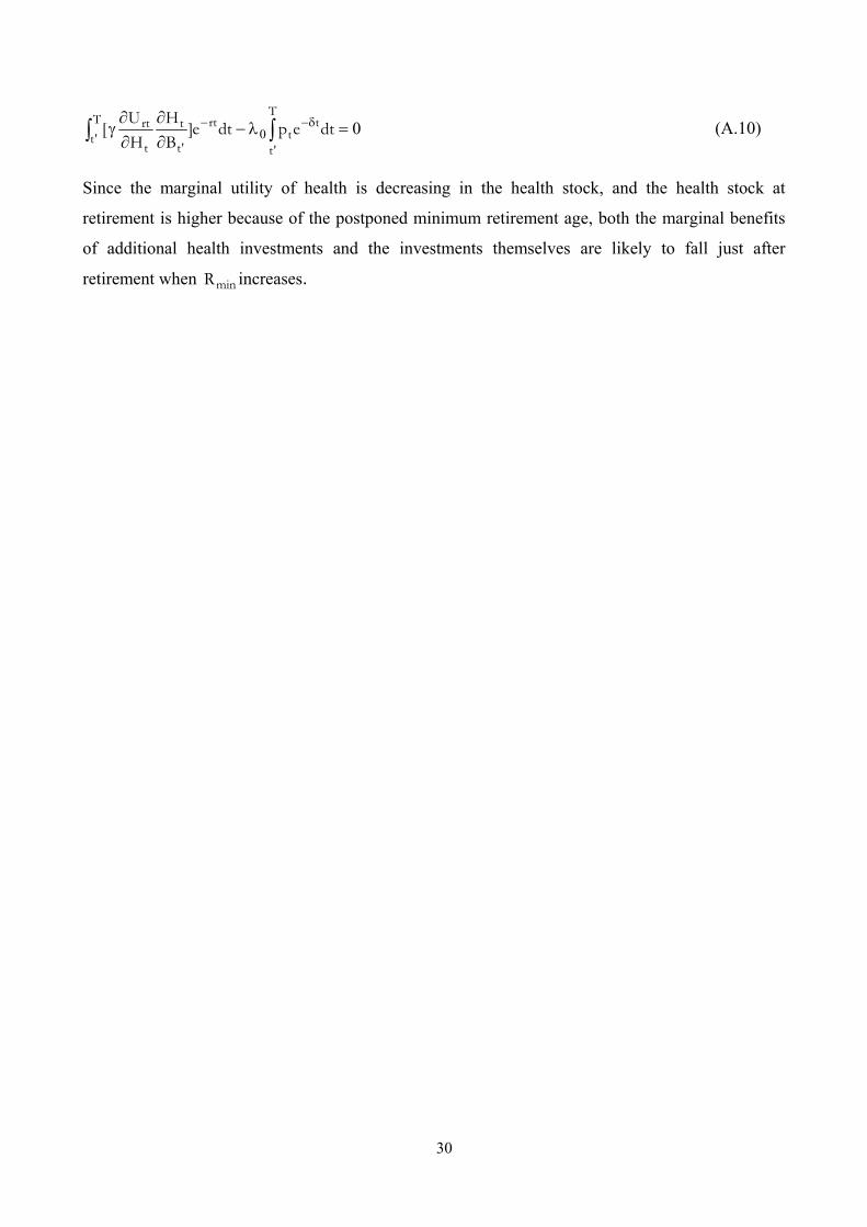
Since the marginal utility of health is decreasing in the health stock, and the health stock at

retirement is higher because of the postponed minimum retirement age, both the marginal benefits

of additional health investments and the investments themselves are likely to fall just after

retirement when minR increases.

31

2. Tables

Table A1. Old-age pension eligibility during the sample period (1997-2011)

Sector: Private Public Self-employedRetirement year: Age & YContr Age & YContr Age & YContr

1997 63+18 65+18 63+18

1998 64+18 65+18 64+18

1999 64+19 65+19 64+19

2000 65+19 65+19 65+19

2001 onwards 65+20 65+20 65+20 Note: Y Contr: years of paid contributions. Table A2. Old-age pension eligibility according to the different reforms in place during the sample period (1997-2011)

a. “Dini” reform. Survey years of application: 1997

Sector: Private Public Self-employed Retirement year: Age & YContr Only YContr Age & YContr Only YContr Age & YContr Only YContr

1997 52&35 36 52+35 36 56+35 40

1998 53&35 36 53&35 36 57&35 40

1999 53&35 37 53&35 37 57&35 40

2000 54&35 37 54&35 37 57&35 40

2001 54&35 37 54&35 37 57&35 40

2002 55&35 37 55&35 37 57&35 40

2003 55&35 37 55&35 37 57&35 40

2004 56&35 38 56&35 38 57&35 40

2005 56&35 38 56&35 38 57&35 40

2006 57&35 39 57&35 39 57&35 40

2007 57&35 39 57&35 39 57&35 40

2008 onwards 57&35 40 57&35 40 57&35 40

b. “Prodi” reform. Years of application: 1998-2004


1998 54&35 36 53&35 36 57&35 40

1999 55&35 37 53&35 37 57&35 40

2000 55&35 37 54&35 37 57&35 40

2001 56&35 37 55&35 37 58&35 40

2002 57&35 37 55&35 37 58&35 40

2003 57&35 37 56&35 37 58&35 40

2004 57&35 38 57&35 38 58&35 40

2005 57&35 38 57&35 38 58&35 40

2006 57&35 39 57&35 39 58&35 40

2007 57&35 39 57&35 39 58&35 40

2008 onwards 57&35 40 57&35 40 58&35 40

32

c. “Maroni” reform. Years of application: 2005-2007


2005 57&35 38 57&35 38 58&35 40 2006 57&35 39 57&35 39 58&35 40 2007 57&35 39 57&35 39 58&35 40 2008 60&35 40 60&35 40 61&35 40 2009 60&35 40 60&35 40 61&35 40 2010 onwards 61&35 40 61&35 40 62&35 40

d. “Prodi bis” reform. Years of application: 2005-2007

Sector: Private Public Self-employed Retirement year:

Age & YContr & (Age+ YContr) Only YContr



2008 58&35 40 58&35 40 59+35 40 2009 59&35&95 40 59&35&95 40 60+35, 96 40 2010 59&35&95 40 59&35&95 40 60+35, 96 40 2011 60&35&96 40 60&35&96 40 61+35, 97 40 2012 60&35&96 40 60&35&96 40 61+35, 97 40 2013 onwards 61&35&97 40 61&35&97 40 62+35, 98 40 Notes: see Table A1. The requirement in terms of (age+ YContr) only applies since 2009

33

Table A3. The effect of years to retirement (PYR) on health behaviours – marginal effects from Probit estimation – linear specification (1) (2) (3) (4) (5) (6) (7) (8)

Sports

regularly Not a

Smoker

No alcohol daily

No red meat daily

Fruit or vegetables

daily

No soft drinks daily

Not obese

Very satisfied

with health

PYR/100 3.78*** 3.82*** 2.46** 2.16* 0.92 2.56* 2.57 2.50** (1.20) (0.96) (1.05) (1.24) (1.19) (1.45) (2.14) (1.16) % effect w.r.t. mean outcome 5.04*** 2.08*** 2.06** .65* .26 .64* .53 3.47** Notes: the table reports the estimated average marginal effects of PYR on the health behaviour listed at the top of each column, obtained from Probit models. The controls included in the regressions reported in this table are those in Table 3 – Panel 1. Results for estimates with a richer set of controls are available from the authors upon request.

Table A4. The effect of potential years to retirement (PYR) on health behaviours – OLS estimation – quadratic specification (1) (2) (3) (4) (5) (6) (7) (8)

Sports

regularly Not a

Smoker

No alcohol daily

No red meat daily

Fruit or vegetable

s daily

No soft drinks daily

Not obese

Very satisfi

ed with

health

PYR/100 0.02 1.57 2.19*** 0.73 -0.18 0.21 0.50 1.23 (0.60) (0.96) (0.79) (0.72) (0.63) (0.63) (1.65) (0.86) PYR/1002 0.05* -0.01 -0.05* -0.01 0.02 0.02 0.00 -0.02 (0.03) (0.03) (0.03) (0.02) (0.02) (0.02) (0.05) (0.03) Notes: see Table 3. The controls included in the regressions reported in this table are those in Table 3 – Panel A. Results for estimates with a richer set of controls are available from the authors upon request.

34

References

Adam, S., Bonsang, E., and Perelman, S., 2012. Does retirement affect cognitive functioning? Journal of Health Economics, 31(3), 490-501.

Angelini, V., Brugiavini, A., and Weber, G., 2009. Ageing and unused capacity in Europe: is there an early retirement trap? Economic Policy, 24(59), 463-508.

Angrist, J. D. and Krueger, A. B., 1992. The effect of age at school entry on educational attainment: An application of instrumental variables with moments from two samples. Journal of American Statistical Association, 87(418), 328-336

Battistin, E., Brugiavini, A., Rettore, E., and Weber, G., 2009. The Retirement Consumption Puzzle: Evidence from a Regression Discontinuity Approach. American Economic Review, 99(5): 2209-26.

Battistin, E., De Nadai, M., and Padula, M., 2014. Roadblocks on the Road to Grandma's House: Fertility Consequences of Delayed Retirement. IZA Discussion Paper n. 8071.

Bertoni, M., Maggi, S. and Weber, G, 2015. Work, retirement and muscle strength loss in old age. Mimeo, University of Padova.

Bertoni, M., and Brunello, G., 2014. Pappa ante Portas: The Retired Husband Syndrome in Japan. IZA DP n. 8350.

Bonsang, E. and Klein, T. J., 2012. Retirement and subjective well-being. Journal of Economic Behavior and Organization, 83(3), 311-329.

Börsch-Supan, A., and Jürges, H., 2009. Early retirement, social security and well-being in Germany. NBER Working Paper n. 12303.

Bottazzi, R., Jappelli, T. and Padula, M., 2006. Retirement expectations, pension reforms, and their impact on private wealth accumulation. Journal of Public Economics, 90 (12), 2187-2212.

Bottazzi, R., Jappelli, T. and Padula, M., 2011. The portfolio effect of pension reforms: evidence from Italy. Journal of Pensions Economics and Finance. 10 (1), 75-97.

Brunello G. and Comi S., 2015, The side effect of pension reforms on the training of older workers. Evidence from Italy. Journal of Economics of Ageing, 113-122.

Cawley J. and Ruhm C., 2011 The economics of risky health behaviors. NBER Working Paper No. w17081.

Celidoni, M., Dal Bianco, C. and Weber, G., 2013. Early retirement and cognitive decline. A longitudinal analysis using SHARE data. “Marco Fanno” Working Paper n. 174, Department of Economics and Management, University of Padua

Celidoni, M., and Rebba, V., 2015. Healthier lifestyles after retirement in Europe? Evidence from SHARE. “Marco Fanno” Working Paper n. 201, Department of Economics and Management, University of Padua

Coe, N. B., and Zamarro, G., 2011. Retirement effects on health in Europe. Journal of Health Economics, 30(1), 77-86.

Charles, K. K., 2004. Is retirement depressing? Labor force inactivity and psychological well-being later in life. Research in Labor Economics, 23, 269-299.

Clark, A. E. and Fawaz, Y., 2009. Valuing jobs via retirement: European evidence. National Institute Economic Review, 209(1), 88-103.

De Grip, A., Lindeboom, M., and Montizaan, R., 2012. Shattered dreams: The effects of changing the pension system late in the game. Economic Journal, 122 (559), 1-25.

Eibich, P., 2015. Understanding the effect of retirement on health: Mechanisms and heterogeneity. Journal of Health Economics, 43, 1-12.

35

Fonseca, R., Kapteyn, A., Lee, J., and Zamarro, G., 2015. Does Retirement Make you Happy? A Simultaneous Equations Approach. A Simultaneous Equations Approach. In: Wise, D.A. (ed.), Insights in the Economics of Aging. Chicago: University of Chicago Press.

Galama, T., Kapteyn, A., Fonseca, R. and Michaud, P. C., 2013, A Health Production Model with Endogenous Retirement, Health Economics, 22, 883-902.

Godard, M., 2016. Gaining weight through retirement? Results from the SHARE study. Journal of Health Economics, 45, 27-46.

Grossman, M., 2000. The human capital model. In: A. J. Culyer & J. P. Newhouse (ed.), Handbook of Health Economics. Elsevier.

Hairault, J. O., Sopraseuth, T., and Langot, F., 2010. Distance to retirement and older workers‘ employment: The case for delaying the retirement age. Journal of the European Economic association, 8(5), 1034-1076.

Imbens, G. W., and Angrist, J. D., 1994. Identification and Estimation of Local Average Treatment Effects. Econometrica, 62(2), 467-475.

Inoue, A., & Solon, G. 2010, Two-sample instrumental variables estimators. The Review of Economics and Statistics, 92(3), 557-561.

Insler, M., 2014. The health consequences of retirement. Journal of Human Resources, 49(1), 195-233.

Johnston, D.W., & Lee, W., 2009, Retiring to the good life? The short-term effects of retirement on health, Economics Letters, 103 (1), 8-11.

Kaempfen, F., & Maurer, J., 2016. Time to burn (calories)? The impact of retirement on physical activity among mature Americans. Journal of Health Economics, 45, 91-102.

Mazzonna, F. & Peracchi, F., 2012. Aging, cognitive abilities and retirement. European Economic Review, 56(4), 691-710.

Mazzonna, F. & Peracchi, F., 2014. Unhealthy retirement? EIEF working paper 09/14 Manacorda, M., & Moretti, E., 2006. Why do Most Italian Youths Live with Their Parents?

Intergenerational Transfers and Household Structure. Journal of the European Economic Association, 4(4), 800–829.

Montizaan R., Cörvers, F., and de Grip, A., 2010. The Effects of Pension Rights and Retirement Age on Training Participation: Evidence from a Natural Experiment. Labour Economics, 2010, 17 (1), 240-247.

Montizaan, R. and Vendrik, M. C. M., 2014. Misery Loves Company: Exogenous Shocks in Retirement Expectations and Social Comparison Effects on Subjective Well-Being. Journal of Economic Behavior and Organization, 97, 1-26.

OECD, 2015. Health at a Glance 2015: OECD Indicators. OECD publishing, Paris. Rohwedder, S., & Willis, R. J. 2010. Mental retirement. The Journal of Economic Perspectives,

24(1), 119. Stock, J. H., Wise, D.A., 1990. The Pension Inducement to Retire: An Option Value Analysis, in

Wise DA (ed.), Issues in the Economics of Ageing, University of Chicago Press, Chicago. Zhao, M., Konishi, Y. and Noguchi, H., 2013. Retiring for Better Health? Evidence from Health

Investment Behaviors in Japan. Waseda University WIAS Discussion Paper no. 20

does postponing minimum retirement age improve …ftp.iza.org/dp9834.pdf · discussion paper series...

Documents