the downside risk of postponing social security benefits
TRANSCRIPT

The Downside Risk of Postponing Social Security Benefits
by
Joseph Friedman
Herbert E. Phillips
Department of Economics
DETU Working Paper 10-08
June 2010
1301 Cecil B. Moore Avenue, Philadelphia, PA 19122
http://www.temple.edu/cla/economics/
The Downside Risk of Postponing Social Security Benefits
Joseph Friedman
Department of Economics
Temple University
Philadelphia, PA 19122
Herbert E Phillips
Department of Finance
Temple University
Philadelphia, PA 19122
Key Words: Social Security, Social Security Benefit
Initiation, Social Security Benefit Postponement, Social
Security Benefit Optimization, Retirement Annuities.
Acknowledgment:
An earlier version of this paper was presented at the AFS/FPA Boston meeting in
October 2008 and received a best paper award.
Abstract
The Downside Risk of Postponing Social Security Benefits
The point that only live participants may initiate or receive Social Security
benefits is typically overlooked. Thus a postponement of benefits at any eligible
retirement age may be likened to participation in a game of chance in which the
participant is subject to a variant form of gambler’s ruin at death. The typical
assumption, therefore, that a participant should automatically opt for a
postponement if the present value of the resulting benefits, discounted to breakeven
age, higher than the present value of the opportunity costs, carries with it the
implication of risk neutrality in relation to the consequence of dying before reaching
breakeven death age. While this implication of risk neutrality is sometimes correct,
it is more likely not. In marked contrast to conclusions reached in previous studies,
this paper shows that a single Social Security participant, who is risk averse as
regards the chances– and contingent consequences– of dying before reaching
breakeven death age, would be well advised to initiate benefits at the earliest age at
which he or she would not be subject to earned income tax penalties.
The Downside Risk of Postponing Social Security Benefits
Joseph Friedman and Hebert E Phillips
1. Introduction
Under current law, the normal retirement age [NRA] for Social Security
participants born between 1943 and 1954 is 66. Participants may claim benefits as
early as early as age 62, which is the presently designated early eligibility age
[EEA], or at any age thereafter– but there is no financial incentive to postpone
benefits beyond age 70.1 Participants who elect to start receiving benefits at the
NRA receive a full retirement benefit [FRB] amount initially, with subsequent
monthly payments increased by an annual inflation adjustment factor. The FRB is
determined by a Principal Insurance Amount [PIA], which the Social Security
Administration calculates on the basis of the number and amount of payments made
into the system prior to the initiation of Social Security Benefits.
1A participant may initiate benefits at the beginning of any month following his or her 62ed
birthday. To simplify the analysis that follows later in the paper, however, we will assume that
initiation versus postponement decisions are made annually, starting at age 62, and that any
participant who has not initiated benefits by age 69 will do so at age 70.
2
The Social Security Administration [SSA] adjusts benefit payments for
Participants who initiate Social Security benefits before or after reaching NRA
relative to the FRB, using adjustment factors that vary by age. The maximum
discount is 25% if benefits are initiated at age 62 and the maximum premium is
32% if initiation takes place at age 70. The delay of benefits by postponement at
any eligible age x, between 62 and 70, therefore, is tantamount to the forfeiture
of a single benefit payment, in exchange for a incremental Social Security benefit
annuity (amount) that will begin one month later and terminate at death.
It is generally assumed that a participant’s decision to initiate benefits or
postpone may result in just two mutually exclusive outcomes: lower lifetime
annuity payments for a longer period of time in the case of initiation or higher
benefit payments for a shorter period of time in the case of postponement. Though
mutually exclusive, these outcomes are not collectively exhaustive. In the case of
postponement there are at least two other possible outcomes:
• A participant may die before initiating benefits, in which case the effective
yield on his or her cumulative postponement investments is -100%.
• A participant may eventually initiate benefits but not live to his or her
3
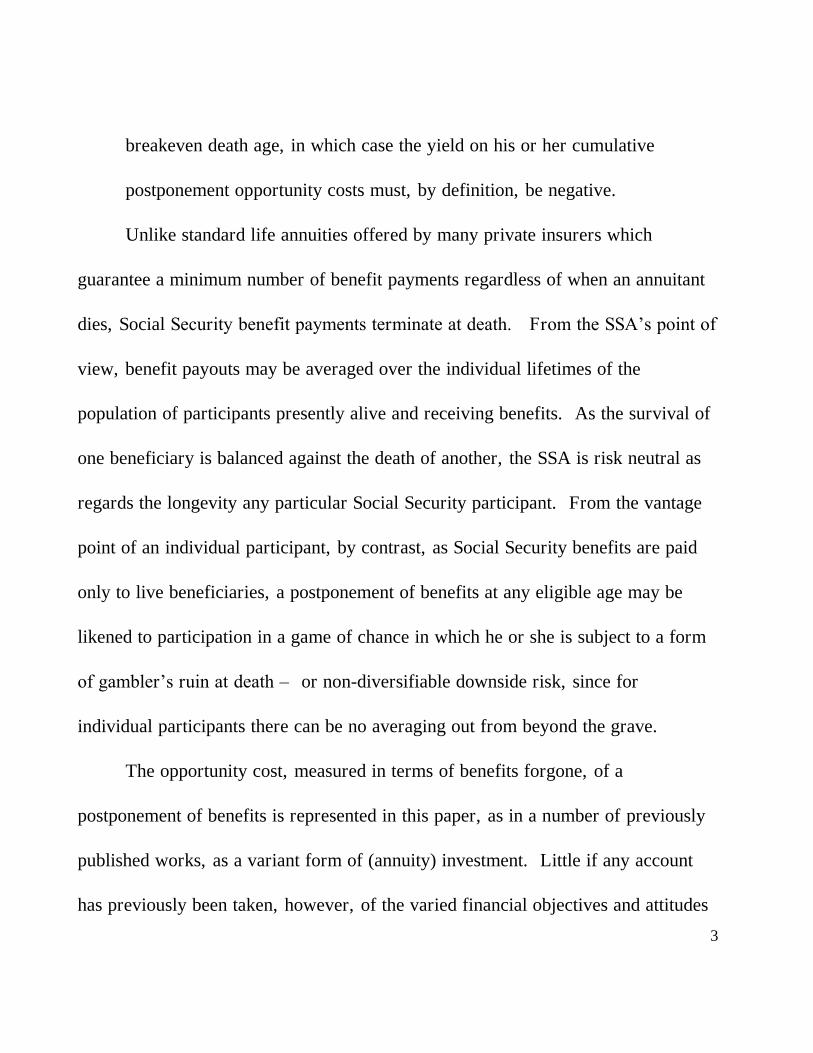
breakeven death age, in which case the yield on his or her cumulative
postponement opportunity costs must, by definition, be negative.
Unlike standard life annuities offered by many private insurers which
guarantee a minimum number of benefit payments regardless of when an annuitant
dies, Social Security benefit payments terminate at death. From the SSA’s point of
view, benefit payouts may be averaged over the individual lifetimes of the
population of participants presently alive and receiving benefits. As the survival of
one beneficiary is balanced against the death of another, the SSA is risk neutral as
regards the longevity any particular Social Security participant. From the vantage
point of an individual participant, by contrast, as Social Security benefits are paid
only to live beneficiaries, a postponement of benefits at any eligible age may be
likened to participation in a game of chance in which he or she is subject to a form
of gambler’s ruin at death – or non-diversifiable downside risk, since for
individual participants there can be no averaging out from beyond the grave.
The opportunity cost, measured in terms of benefits forgone, of a
postponement of benefits is represented in this paper, as in a number of previously
published works, as a variant form of (annuity) investment. Little if any account
has previously been taken, however, of the varied financial objectives and attitudes
4
towards risk of individual participants when contemplating such postponement of
benefits investment decisions. Indeed, the common assumption– that a participant
will or should opt for postponement if the present value of the incremental benefits,
discounted to life expectancy, is higher than the present value of the benefits
forgone– carries with it the implication of risk neutrality in relation to the
probability of dying before reaching breakeven death age.
While the assumption of risk neutrality by an insurance company might be
perfectly reasonable, the normative implications of a risk neutrality assumption –
whether by explicit assertion or by implication– are inconsistent with now standard
investment theory precepts regarding individual behavior in the face of uncertain
outcomes, and attitudes towards risk. Accordingly, the investment objectives and
behavior of individual Social Security participants would seem better characterized
by risk aversion.2
This paper shows that the downside risk associated with the postponement of
benefits by any single participant– of either gender and/or at any eligible age– is an
order of magnitude higher than the potential gain. In the case of a single Social
2By definition, a risk adverse individual is simply one who is made happy by anticipation of
gain but is vexed by uncertainty.

5
Security participant who is risk averse as regards the consequence of dying before
reaching breakeven death age, therefore, it follows that he or she would be well
advised to initiate benefits at the earliest age at which she or he would not be
subject to earned income tax penalties. Postponement of benefits versus initiation
decisions made by married couples are, in general, more complex, and the
implications of risk aversion– which may depend on a myriad of possible unique
contingencies– therefore are less clear cut. The married couple issue was taken up
in a recent paper by Munnell and Soto (2007) but is not formally addressed in this
paper.
2. Review of Recent Literature
Cook, Jennings, and Reichenstein (2002) calculate the present values of SSA
benefit streams, discounted at 3% to life expectancy, categorized by initiation age.
They identify the initiation ages for single male and single female participants,
respectively, that maximize the present values of the expected benefit streams, then
contrast these results– for males and females separately– with the calculated present
value obtained for each alternative initiation age, and conclude that the SSA’s
actuarial benefit adjustments are fair and that that it makes no difference at what
age a beneficiary initiates benefits.
6
Detweiler (1999) considers multiple real rates return and investment
scenarios. He defines negative cash flow as being created by initiation at age 62
and positive cash flow as being created by initiation at the NRA, which at the time
of his study was age 65, and breakeven death age as the time of death at which a
net present value to life expectancy function would go to zero. Based on this logic
he calculates breakeven death ages under a variety of different real interest rate
assumptions, and accounts for the probability of dying at or before one’s breakeven
death age using cumulative distribution mortality data. Restricting his analysis to
individuals who will invest their benefits rather than spend them and who feel
comfortable managing their own investments, he concludes that a male beneficiary
whose expected real rate of return on investments is in excess of approximately
2.25% should probably initiate benefits at age 62, but that a female would require
an expected real rate of return in excess of approximately 4.5% to justify doing so.
Like Detweiler (1999), Spitzer (2006) considers multiple real rates return,
but he also attempts to account for the stochastic nature of rates of return, and their
relationship to alternative financial market conditions and asset allocation strategies.
He performs breakeven analyses for unmarried single male and single female
participants, born between 1943 and 1954, contemplating initiation at age 62 or 66.

7
His results indicate that postponement is more easily justified for female than male
participants because of longer life expectancy, but for either group– all other things
equal– the breakeven initiation age is later the higher discount rate and/or the later
the beneficiary’s age at initiation.
McCormack and Perdue (2006) first consider the case of single male and
female participants, born in 1943, who at age 62 will decide whether to initiate at
age 62, 66, or 70. The analysis is then extended to married couples. Having taken
note of the stochastic implications of a median life expectancy statistic by
referencing a paper by Milevsky, Kwok and Robinson (1997) that reminds us, in
effect, that the median marks the 50th percentile of a distribution, calculate internal
rates of return using a present value to life expectancy model using five percentiles
of a cumulative life expectancy distribution for single male and single female
participants. They explicitly assume, however, that, in each case, the beneficiary
will live to an age commensurate with life expectancy, receive benefits to that date,
and nothing more thereafter.
Munnell and Soto (2007) discuss initiation decision issues confronting
married participants. This situation is more complex. A married women may, for
example, receive benefits based on her own contributions starting at age 62, but can
8
trade her benefit for a maximum of 50% of her husband’s adjusted benefit when he
initiates, provided that her adjusted benefit does not exceed 50% of his. A married
woman at or beyond age 62, by contrast, who would not qualify for benefits on her
own nevertheless qualifies to receive a spousal benefit equal to a maximum of 50%
of her husband’s adjusted benefit. Either way, spousal benefits are subject to
actuarial adjustment depending on the wife’s age when and if she initiates. Upon a
husband’s death, however, regardless of the wife’s age when he passes, she is
entitled to 100% of her husband’s benefits in exchange for her own benefit or
spousal benefit. These authors conclude that a wife with a living and healthy
spouse who happens to be the same age as she, will typically be better off initiating
early. The husband, on the other hand, should take into account not only his own
expected benefit stream over his lifetime, but also the impact that his age on
initiation decision will have on his wife’s spousal and/or contingent benefit streams.
Accordingly, the authors argue, that married men should typically initiate later.
Friedman and Phillips (2008) invoke the same behavioral assumptions as in
the preceding papers, which imply risk neutrality, but replace the discreet
aggregative approaches employed by Detweiler (1999), Spitzer (2006), and
McCormack and Perdue (2006), respectively, with a sequential model that views an

9
initiation versus postponement analysis as an iterative process that plays out over
time. According to this sequential approach, which is also employed in this paper,
the question asked at each decision point is not whether to initiate at that point or
postpone until some critical age, such as 62, 66, or 70, but whether to initiate now
or postpone for just one year. By means of this sequential model, Friedman and
Phillips (2008) conclude that the minimum investment yield required to justify
initiation at any eligible age varies from one eligible retirement age to the next, and
that while early initiation might me beneficial at one age it might not be at the next.
This oscillation is not duplicated this paper– where downside risk and risk aversion
are explicitly taken into account.. .
3. Background, Issue, and Model
A participant may initiate benefits at age 62, or, failing to do so, may revisit
his or her initiation versus postponement decision one month later, and each month
after that until the decision to initiate benefits is made or death occurs– whichever
comes first. As only a live participant can initiate or receive Social Security
benefits, previous works that cast a participant contemplating a postponement of
benefits versus initiation decision as an unbridled present value or yield on
investment maximizer– one who would or should opt for postponement if the

10
present value of the incremental benefits discounted to life expectancy is higher than
the present value of the benefits forgone– carry the implications of participant risk
neutrality as regards the non-diversifiable downside risk of dying before reaching
breakeven death age.
3.1 The Issue
Though the assumption of risk neutrality is never explicitly stated, and in the
past may never have been intended, this implication may, nevertheless, be
appropriate in some cases– though we believe that this would be the exception
rather than the rule. Consider, for example, the case of a reasonably affluent,
unattached, “after me the flood” type of individual: it seems reasonable to suppose
that such a person– while not indifferent to dying– might be indifferent to the
downside risk of dying before reaching breakeven death age, as previously defined.
Such unbridled self-centeredness is not a prerequisite for downside risk neutrality
however. An active investor, for example, with significant holdings outside the
Social Security system may view the return on a traditional Social Security account
as return on a riskless asset. Accordingly, as explained by Friedman and Phillips
(2009), a guaranteed (for life) benefit plan, in the framework of a total retirement
portfolio analysis, may be valued more for its contributions to the reduction of

11
diversifiable risk than as a source of retirement income or estate wealth. In this
framework of total portfolio diversification, paradoxically, an investor/participant
might simultaneously be risk averse as regards risk-return tradeoffs on a total
retirement portfolio and risk neutral as regards the downside risk of dying before
reaching breakeven death age. The operative word, of course, is “might;” there is
no reason to suppose that every participant with financial holdings outside the
Social Security system is efficiently diversified– in the sense fashioned by
Markowitz (1952)– or subscribes to this investment logic.
3.2. The model
The model assumes that a Social Security participant views the initiation
versus postponement of benefits decision process as a sequential decision process,
started at age 62 and revisited annually, on the occasion of each subsequent
birthday, until the decision is made to initiate benefits or the beneficiary dies–
whichever comes first.3 The incremental cost of postponing benefits at any age,
therefore, is measured in terms of the benefits sacrificed in that single year.4
3Please see footnote 1.
4It might be argued that each monthly incremental cost-benefit tradeoff should be
considered, but this would be neither beneficial nor practical. As SSA benefit and cost of living
12
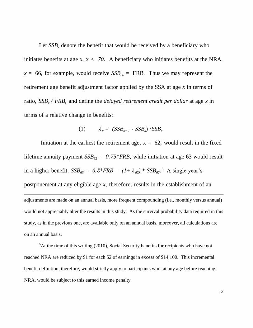
Let SSBx denote the benefit that would be received by a beneficiary who
initiates benefits at age x, x < 70. A beneficiary who initiates benefits at the NRA,
x = 66, for example, would receive SSB66 = FRB. Thus we may represent the
retirement age benefit adjustment factor applied by the SSA at age x in terms of
ratio, SSBx / FRB, and define the delayed retirement credit per dollar at age x in
terms of a relative change in benefits:
(1) λ x = (SSBx+ 1 - SSBx) /SSBx
Initiation at the earliest the retirement age, x = 62, would result in the fixed
lifetime annuity payment SSB62 = 0.75*FRB, while initiation at age 63 would result
in a higher benefit, SSB63 = 0.8*FRB = (1+ λ 62) * SSB62.5 A single year’s
postponement at any eligible age x, therefore, results in the establishment of an
adjustments are made on an annual basis, more frequent compounding (i.e., monthly versus annual)
would not appreciably alter the results in this study. As the survival probability data required in this
study, as in the previous one, are available only on an annual basis, moreover, all calculations are
on an annual basis.
5At the time of this writing (2010), Social Security benefits for recipients who have not
reached NRA are reduced by $1 for each $2 of earnings in excess of $14,100. This incremental
benefit definition, therefore, would strictly apply to participants who, at any age before reaching
NRA, would be subject to this earned income penalty.
13
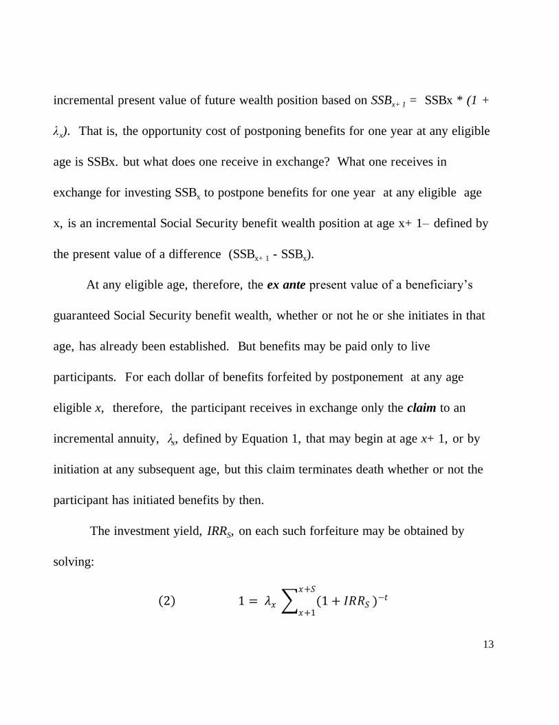
incremental present value of future wealth position based on SSBx+ 1 = SSBx * (1 +
λ x). That is, the opportunity cost of postponing benefits for one year at any eligible
age is SSBx. but what does one receive in exchange? What one receives in
exchange for investing SSBx to postpone benefits for one year at any eligible age
x, is an incremental Social Security benefit wealth position at age x+ 1– defined by
the present value of a difference (SSBx+ 1 - SSBx).
At any eligible age, therefore, the ex ante present value of a beneficiary’s
guaranteed Social Security benefit wealth, whether or not he or she initiates in that
age, has already been established. But benefits may be paid only to live
participants. For each dollar of benefits forfeited by postponement at any age
eligible x, therefore, the participant receives in exchange only the claim to an
incremental annuity, λx, defined by Equation 1, that may begin at age x+ 1, or by
initiation at any subsequent age, but this claim terminates death whether or not the
participant has initiated benefits by then.
The investment yield, IRRS, on each such forfeiture may be obtained by
solving:
2 1 = 𝜆𝑥 (1 + 𝐼𝑅𝑅𝑆 )−𝑡
𝑥+𝑆
𝑥+1

14
for any S, where S denotes the number of years beyond age x (the age at which a
forfeiture was made) that the participant survives. But benefits may be initiated
only by live participants. If a participant dies before reaching age x+ 1, therefore,
or before initiating benefits at any subsequent eligible age, then the ex post
investment yield, IRRS, on each postponement forfeiture, and/or on the total of all
such forfeitures, is -100%.
For reasons that will be made clear below, we call IRRS the unweighted
yield on a one period postponement made at age x by a beneficiary who survives to
age x+ S. The average unweighted yield on a postponement decision made at age x
[AUWYx] may then be calculated as follows:
(3) 𝐴𝑈𝑊𝑌𝑥 = 𝐼𝑅𝑅𝑆
100−𝑥
𝑆=0/(100 − 𝑥)
A single individual in poor health at any age would generally have no incentive to
postpone benefits and a beneficiary older than 70 would never have an incentive to
do so. An individual at any eligible age x, who is in good health, by contrast,
would nevertheless have no way of knowing when the end of life will come. In the
case of outwardly healthy individuals, therefore, prior estimates of death age are
15
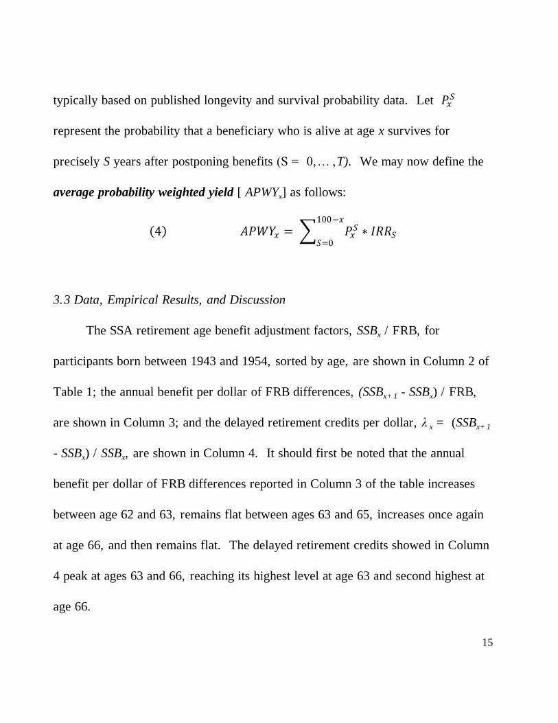
typically based on published longevity and survival probability data. Let 𝑃𝑥𝑆
represent the probability that a beneficiary who is alive at age x survives for
precisely S years after postponing benefits (S = 0,… ,T). We may now define the
average probability weighted yield [ APWYx] as follows:
4 𝐴𝑃𝑊𝑌𝑥 = 𝑃𝑥𝑆
100−𝑥
𝑆=0∗ 𝐼𝑅𝑅𝑆
3.3 Data, Empirical Results, and Discussion
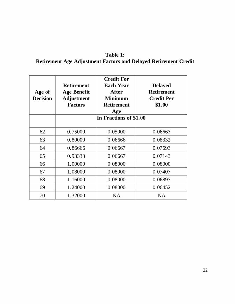
The SSA retirement age benefit adjustment factors, SSBx / FRB, for
participants born between 1943 and 1954, sorted by age, are shown in Column 2 of
Table 1; the annual benefit per dollar of FRB differences, (SSBx+ 1 - SSBx) / FRB,
are shown in Column 3; and the delayed retirement credits per dollar, λ x = (SSBx+ 1
- SSBx) / SSBx, are shown in Column 4. It should first be noted that the annual
benefit per dollar of FRB differences reported in Column 3 of the table increases
between age 62 and 63, remains flat between ages 63 and 65, increases once again
at age 66, and then remains flat. The delayed retirement credits showed in Column
4 peak at ages 63 and 66, reaching its highest level at age 63 and second highest at
age 66.

16
TABLE 1 GOES APPROXIMATELY HERE
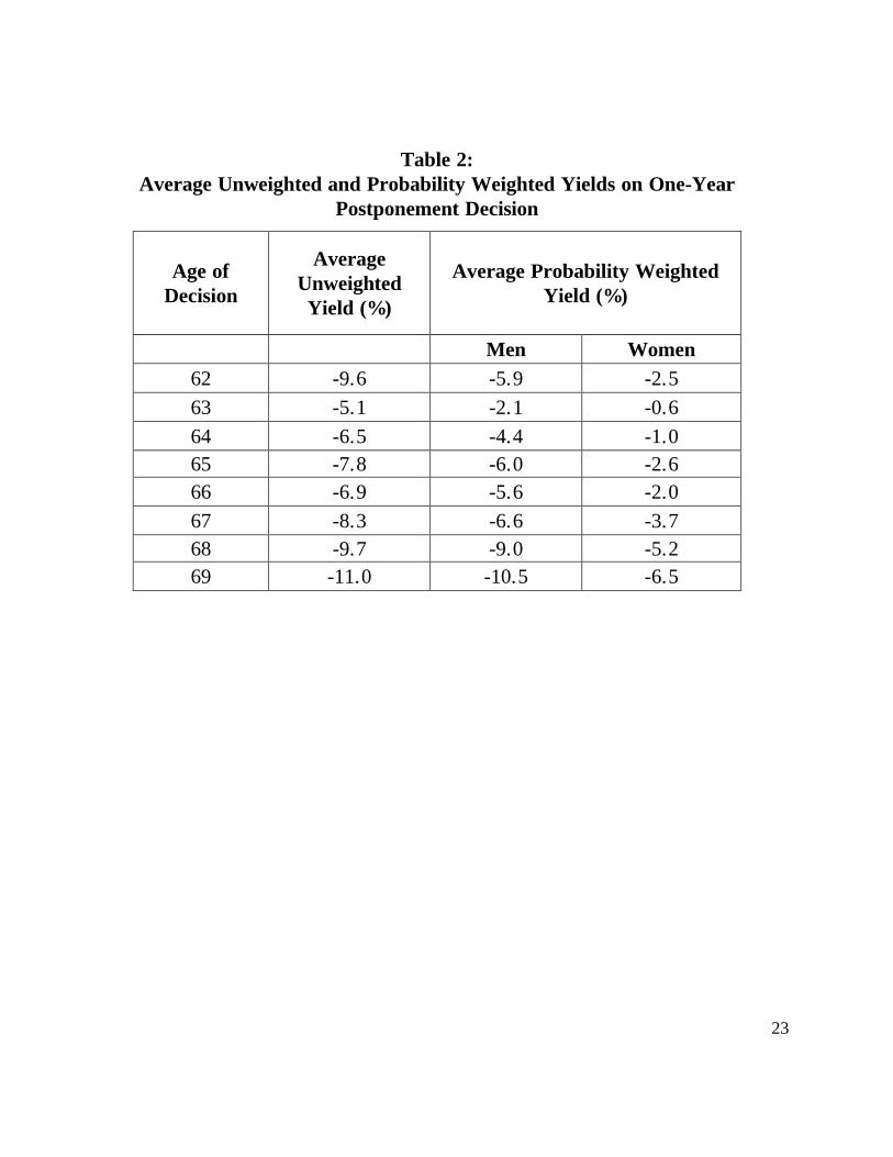
The delayed retirement credits shown in Column 4 of Table 1 were used in
equation (3) to calculate the unweighted yields, IRRS, S = 0, . . . , (100-x). The
AUWYx, and the APWYx, for males and females, separately, for one-year
postponement decisions, were then calculated using equations (4) and (5)
respectively. The results are reported in Table 2.
TABLE 2 GOES APPROXIMATELY HERE
Table 2 suggests that a postponement of Social Security benefits at any
eligible age is more akin to a crap-shoot than a prudent financial investment. Even
before accounting for beneficiary’s survival probabilities, we see from Column 2 of
the table that the Average Unweighted Yield on a one-period postponement is
negative at any age x, fluctuates between ages 62 and 65, but is monotonic
decreasing beyond age 65. What explains this? It should first be noted that a
beneficiary’s yield on a postponement decision made at any age x will be -100% if
he or she dies before the first payment is received; that is if she or he does not
survive to age x+ 1. 6 Indeed, by definition, IRRS is negative until one reaches the
6If this annual analysis were replaced by a monthly analysis, the up-front losses would be of
the same order of magnitude and the table would simply be longer.
17
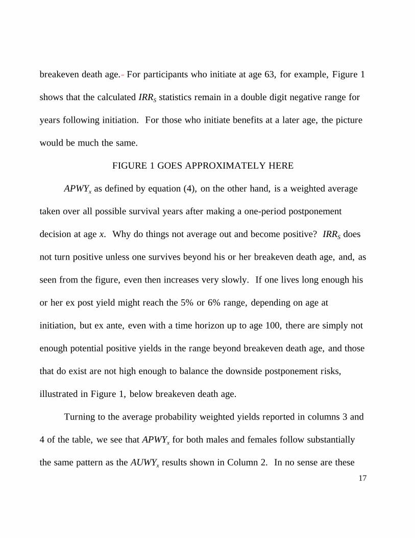
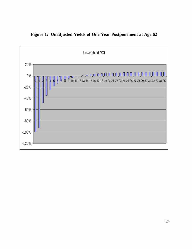
breakeven death age. For participants who initiate at age 63, for example, Figure 1
shows that the calculated IRRS statistics remain in a double digit negative range for
years following initiation. For those who initiate benefits at a later age, the picture
would be much the same.
FIGURE 1 GOES APPROXIMATELY HERE
APWYx as defined by equation (4), on the other hand, is a weighted average
taken over all possible survival years after making a one-period postponement
decision at age x. Why do things not average out and become positive? IRRS does
not turn positive unless one survives beyond his or her breakeven death age, and, as
seen from the figure, even then increases very slowly. If one lives long enough his
or her ex post yield might reach the 5% or 6% range, depending on age at
initiation, but ex ante, even with a time horizon up to age 100, there are simply not
enough potential positive yields in the range beyond breakeven death age, and those
that do exist are not high enough to balance the downside postponement risks,
illustrated in Figure 1, below breakeven death age.
Turning to the average probability weighted yields reported in columns 3 and
4 of the table, we see that APWYx for both males and females follow substantially
the same pattern as the AUWYx results shown in Column 2. In no sense are these

18
results consistent with the previously published and widely held view that, by virtue
of longer life expectancy, females should initiate later than males. On the contrary,
Table 2 suggests, all other things equal, that the postponement of Social Security
benefits by any risk averse participant, who is not indifferent to the downside risk
of dying before reaching breakeven death age, would be a poor bet at any eligible
age regardless of gender, but that single males suffer greater losses on average than
single females. This analysis cannot be easily extended to married couples, for
reasons explained by Munnell and Soto (2007).
Finally, contrasting the difference between AUWYx and APWYx , at any age
and for either gender, we see that the differences are monotonic decreasing with
age for males, but are relatively constant beyond NRA for females. It is intuitively
obvious that because females live longer on average than men, a proportionately
greater number survive to and beyond their breakeven death age than their male
counterparts, and that there are relatively more old age outliers among females than
males.
19
4. Conclusions
Previously published papers that contrast the financial implications of
initiation versus postponement decisions, by employing quite different assumptions
about participant behavior, decision prerogatives, and attitudes towards risk, reach
very different conclusions than those arrived at in the present study. We did not
miss the point in our previous study that benefits are paid only to live participants, 7
but we did overlook the relationship between downside financial risk and one’s
prior uncertainty about when he or she might die.
In light of this prior uncertainty about death age, the decision to postpone
benefits at any eligible age may be likened to participation in a game of chance in
which the beneficiary is subject to a variant form of gambler’s ruin at death. The
same law of large numbers that applies to an insurer or the SSA, therefore, that
calculates averages taken over the lives of many individuals, does not also apply to
an individual participant– for whom there can be no averaging out from beyond the
grave.
The breakeven age was defined as the age at which the present value of the
benefits resulting from postponement is just equal to the opportunity cost of
7See Friedman and Phillips (2008).
20
postponement. It may seem intuitively obvious that the longer one postpones the
initiation of benefits, the later is breakeven age, and the less likely that he or she
will live so long. This is in the nature of risk, but it does not fully explain the
downside risk envisaged in this paper. As explained above and illustrated in
Figure 1, even for participants who survive to their breakeven ages and beyond,
there will not be enough high positive yields to offset the high negative yields that
would result from dying before reaching breakeven age. The downside risk is
explained by two factors: The high negative yields that would be realized by
participants who may not survive to their breakeven ages and by the ex ante
financial reward that is too small to compensate those who manage to live beyond
their breakeven ages.
The major conclusion reached in this paper is that risk adverse participants
would be advised to claim their Social Security benefits as soon as they would not
be subject to the earned income benefit penalty
.

21
References
Cook, K. A., Jennings, W.W., and Reichenstein, W. (2002). “When Should You
Start Your Social Security Benefits?” AAII Journal, 24, 27-34.
Detweiler, J. H. (1999). “A note on the 62-65 Social Security Decision.” National
Estimator, Spring, 39-42.
Friedman, J. , and H.E. Phillips (2008), “Optimizing Social Security Benefit
Initiation and Postponement Decisions: A Sequential Approach.” Financial
Services Review, 17, 155-168.
Friedman, J., and H. E. Phillips (2009), “The Portfolio Implications of Adding
Social Security Private Account Options to Ongoing Investments.“ Financial
Services Review, 18, 333-353.
Jennings, W., and W. Reichenstein (2001), “Estimating the Value of Social
Security Benefits.” Journal of Wealth Management, 4, 14 -29.
Markowitz, H.M., (1952). “Portfolio Selection.” Journal of Finance, 7, 77-91.
McCormack J. M., and G. Perdue (2006), “Optimizing the Initiation of Social
Security Benefits.” Financial Services Review, 15, 335-348.
Munnell A. H., and M. Soto (2007). “When Should Women Claim Social Security
Benefits?” The Journal of Financial Planning, 20, 58-65.
Spitzer, J. J. , (2006). Delaying Social Security Payment: A Bootstrap.” Financial
Services Review, 15, 233-245.
22
Table 1:
Retirement Age Adjustment Factors and Delayed Retirement Credit
Age of
Decision
Retirement
Age Benefit
Adjustment
Factors
Credit For
Each Year
After
Minimum
Retirement
Age
Delayed
Retirement
Credit Per
$1.00
In Fractions of $1.00
62 0.75000 0.05000 0.06667
63 0.80000 0.06666 0.08332
64 0.86666 0.06667 0.07693
65 0.93333 0.06667 0.07143
66 1.00000 0.08000 0.08000
67 1.08000 0.08000 0.07407
68 1.16000 0.08000 0.06897
69 1.24000 0.08000 0.06452
70 1.32000 NA NA
23
Table 2:
Average Unweighted and Probability Weighted Yields on One-Year
Postponement Decision
Age of
Decision
Average
Unweighted
Yield (%)
Average Probability Weighted
Yield (%)
Men Women
62 -9.6 -5.9 -2.5
63 -5.1 -2.1 -0.6
64 -6.5 -4.4 -1.0
65 -7.8 -6.0 -2.6
66 -6.9 -5.6 -2.0
67 -8.3 -6.6 -3.7
68 -9.7 -9.0 -5.2
69 -11.0 -10.5 -6.5
24
Figure 1: Unadjusted Yields of One Year Postponement at Age 62
Unweighted ROI
-120%
-100%
-80%
-60%
-40%
-20%
0%
20%
0 1 2 3 4 5 6 7 8 9 10 11 12 13 14 15 16 17 18 19 20 21 22 23 24 25 26 27 28 29 30 31 32 33 34 35