domain decomposition methods for parallel

INTERNATIONAL JOURNAL FOR NUMERICAL METHODS IN ENGINEERING

Int. J. Numer. Meth. Engng. 44, 281—303 (1999)

DOMAIN DECOMPOSITION METHODS FOR PARALLELSOLUTION OF SHAPE SENSITIVITY ANALYSIS PROBLEMS

MANOLIS PAPADRAKAKIS* AND YIANNIS TSOMPANAKIS

Institute of Structural Analysis and Seismic Research, National Technical University of Athens, Athens 15773, Greece

ABSTRACT

This paper presents the implementation of advanced domain decomposition techniques for parallel solutionof large-scale shape sensitivity analysis problems. The methods presented in this study are based on theFETI method proposed by Farhat and Roux1 which is a dual domain decomposition implementation. Twovariants of the basic FETI method have been implemented in this study: (i) FETI-1 where the rigid-bodymodes of the floating subdomains are computed explicitly. (ii) FETI-2 where the local problem at eachsubdomain is solved by the PCG method and the rigid-body modes are computed explicitly. A two-leveliterative method is proposed particularly tailored to solve re-analysis type of problems, where the dualdomain decomposition method is incorporated in the preconditioning step of a subdomain global PCGimplementation. The superiority of this two-level iterative solver is demonstrated with a number ofnumerical tests in serial as well as in parallel computing environments. Copyright ( 1999 John Wiley& Sons, Ltd.

KEY WORDS: shape sensitivity analysis; domain decomposition methods; preconditioned conjugate gradient; multipleright-hand sides; reanalysis problems

INTRODUCTION

Shape optimization aims to improve the shape of a structure, defined with a number ofparameters called design variables, by minimizing an objective function subject to certainconstraint functions. The shape optimization algorithm proceeds with the following steps: (i)a finite element mesh is generated, (ii) displacements, stresses, frequencies, etc. are evaluateddepending on the type of optimization problem, (iii) the gradients, or the sensitivities of thefunctions are computed by perturbing each design variable by a small amount, (iv) the optimiza-tion problem is solved and the new shape of the structure is defined. These steps are repeated untilconvergence has occurred. The most time-consuming part of a gradient-based optimizationprocess is devoted to the sensitivity analysis phase. For this reason several techniques have beendeveloped for the efficient calculation of the sensitivities in an optimization problem. Thesemi-analytical and the finite-difference approaches are the two most widely used types ofsensitivity analysis techniques. From the algorithmic point of view the semi-analytical techniqueresults in a typical linear solution problem with multiple right-hand sides in which the stiffness

*Correspondence to: Manolis Papadrakakis, Department of Civil Engineering, National Technical University, ZografouCampus, GR 157 73 Athens, Greece. E-mail: [email protected]

Contract/grant sponsor: European Union; Contract/grant number: HC&M/9203390

CCC 0029—5981/99/020281—23$17.50 Received 24 June 1996Copyright ( 1999 John Wiley & Sons, Ltd. Revised 20 February 1998

matrix remains the same, while the finite-difference technique results in a typical re-analysisproblem in which the stiffness matrix is modified due to the perturbations of the design variables.

Shape optimization problems are usually computationally intensive tasks, where 60—90per cent of the computations are spent for the solution of equilibrium equations required for thefinite element analysis and sensitivity analysis. Although it is widely recognized that hybridsolution methods, based on a combination of direct and iterative solvers for solving linear finiteelement equations, outperform their direct counterparts, in sequential as well as parallel comput-ing environments, little effort has been devoted until now to their implementation in the field ofstructural optimization. In a recent paper by Papadrakakis et al.,2 the performance of variousiterative solution methods, based on PCG and Lanczos algorithms, in sequential computingenvironment was demonstrated and compared with the conventional direct skyline solver ina number of topology and shape optimization problems. In the present study two variants of thebasic FETI method of Farhat and Roux1 are implemented for solving sensitivity analysisproblems using the semi-analytical approach, while an innovative two-level parallel solutionmethod is proposed for solving sensitivity analysis problems using the global finite-differenceapproach.

In the two variants of the basic FETI method the rigid-body modes of the floating subdomainsare computed explicitly, while in the second variant a PCG iterative solver with a strongpreconditioner is also used for the solution of the local problem in each subdomain. These twovariants have a beneficial effect on the robustness of basic FETI method for ill-conditionedproblems, while the second variant operates under reduced storage requirements.3 In the presentstudy a two-level iterative method is proposed specially tailored for solving reanalysis type ofproblems in general, a special case of which is the problem arising when the global finite-difference sensitivity analysis approach is used. For this type of problems the two variants of thebasic FETI method are incorporated in the preconditioning step of a global subdomain imple-mentation of the PCG method. This two-level subdomain implementation is applicable in serialand parallel computing environments resulting in a drastic improvement of computing timecompared to the conventional one-level methods.

SHAPE SENSITIVITY ANALYSIS

Sensitivity analysis is the most important and time-consuming part of gradient-based structuraloptimization. Several techniques have been developed which can be mainly distinguished by theirnumerical efficiency and their implementation aspects. The primary objective of sensitivityanalysis is to compute the derivatives of the displacement field with respect to perturbations of theprimary design variables.4 The methods for sensitivity analysis can be divided into discrete andvariational methods.5 In the variational approach the sensitivity coefficients can be determinedby applying basic variational theorems. In this case, the sensitivities are given as boundary andsurface integrals which are solved after the structure has been discretized, whereas in the discreteapproach they are evaluated using the finite element equations. The implementation for dis-crete methods is simpler than the one for variational techniques. A further classification of thediscrete methods is the following:4 (i) Global finite-difference method where the derivatives neededfor the solution of the optimization problem are computed numerically. (ii) Semi-analyticalmethod where the calculation of the sensitivities is performed via analytical and numericalexpressions. (iii) Analytical method where the derivatives of the objective and constraint functionsare obtained analytically.

282 M. PAPADRAKAKIS AND Y. TSOMPANAKIS

Copyright ( 1999 John Wiley & Sons, Ltd. Int. J. Numer. Meth. Engng. 44, 281—303 (1999)

The decision on which method to implement depends strongly on the type of problem, theorganization of the computer program and the access to the source code. The implementation ofanalytical and semi-analytical methods is more complex and requires access to the source code,whereas when a finite-difference method is applied the formulation is much simpler. Dependingon the type of problem and the approach used, the sensitivity analysis together with the finiteelement analysis can take 60—90 per cent of the total computational effort required to solve thewhole optimization problem. An efficient and reliable sensitivity analysis module that can takefull advantage of the innovative computer architectures with parallel processing capabilitiescould therefore result in a considerable reduction of the overall computational effort of theoptimization procedure. In the present study the emphasis is given on the application of efficientdomain decomposition methods in parallel computing environments for solving the systems ofthe algebraic equations encountered in the two most commonly used types of sensitivity analysis,namely the global finite difference and the semi-analytical approaches.

¹he Global Finite-Difference (GFD) approach

The GFD approach provides a simple way of computing the sensitivity coefficients. Thismethod requires the solution of the linear system of equations Ku"f, where u is thedisplacement vector, for the original design variables s0, and for each perturbed design variablespk"s0

k#*s

k, where *s

kis the magnitude of the perturbation, usually taken in the range of

10~3—10~5 of the value of the design variable. The design sensitivities for the displacementsLu/Ls

kare computed using a forward difference scheme:

Lu/Lsk+

*u

*sk

"

u (sk#*s

k)!u (s

k)

*sk

(1)

where u(sk#*s

k) is evaluated by solving the following reanalysis type of problem:

K(sk#*s

k)u (s

k#*s

k)"f (s

k#*s

k) (2)

The Semi-Analytical (SA) approach

The SA approach is based on the chain rule differentiation of the finite element equationsKu"f :

KLu

Lsk

#

LK

Lsk

u"L f

Lsk

(3)

which when rearranged results in

KLu

Lsk

"f *k

(4)

where

f *k"

L f

Lsk

!

LK

Lsk

u (5)

DOMAIN DECOMPOSITION METHODS FOR PARALLEL SOLUTION 283


f *k

represents a pseudo-load vector. The derivatives of LK/Lskand Lf /Ls

kare computed for each

design variable by recalculating the new values of K(sk#*s

k) and f (s

k#*s

k) for a small

perturbation *skof the design variable s

k, while the stiffness matrix remains unchanged through-

out the whole sensitivity analysis.

The Conventional Semi-Analytical (CSA) approach. In the CSA approach, the values of thederivatives in equation (3) are calculated by applying the forward-difference approximation

LK/Lsk+

*K

*sk

"

K (sk#*s

k)!K (s

k)

*sk

(6)

Lf/Lsk+

* f

*sk

"

f (sk#*s

k)!f (s

k)

*sk

(7)

For maximum efficiency of the semi-analytical approach only those elements which are affectedby the perturbation of a certain design variable are involved into the calculations of L f/Ls

kand

LK/Lsk.

The *Exact+ Semi-Analytical (ESA ) approach. The CSA approach may suffer some drawbacks inparticular types of shape optimization problems. This is due to the fact that in the numericaldifferentiation of the element stiffness matrix with respect to shape design variables the compo-nents of the pseudo-load vector associated with the rigid-body rotation do not vanish. Thesolution suggested by Olhoff et al.6 alleviates the problem by performing an ‘exact’ numericaldifferentiation of the elemental stiffness matrix as follows:

Lk

Lsk

"

n+j/1

Lk

Laj

Laj

Lsk

(8)

where n is the number of elemental nodal coordinates affected by the perturbation of the designvariable s

kand a

jis the nodal co-ordinate of the element which can be either an x- or

a y-co-ordinate. This means that by perturbing a design variable all nodes of an element on theperturbed boundary are perturbed as well and the summation is carried out only for theperturbed nodal co-ordinates. The term La

j/Ls

kis computed using the forward-difference

scheme while the derivative Lk/Lajis computed by differentiating the element stiffness matrix

expression.

SOLUTION METHODS IN SENSITIVITY ANALYSIS PROBLEMS

The implementation of hybrid solution schemes in structural optimization, which are based ona combination of direct and preconditioned iterative solvers, has not yet received the attention itdeserves from the research community, even though in finite element linear solution problemsand particularly when dealing with large-scale applications their efficiency is well documented. Ina recent study by Papadrakakis et al.,2 a class of efficient hybrid solution methods was applied inthe context of shape sensitivity analysis and topology optimization problems in sequentialcomputing environment.



In this work domain decomposition methods are applied for solving the sensitivity analysispart of shape optimization problems, in both sequential and parallel computing environments,after being properly modified to address the special features of the particular type of problems athand. The most computational intensive part of sensitivity analysis, using either semi-analyticalor finite-difference sensitivity analysis approaches, is the solution of finite element equilibriumequations (4) or (2), respectively. In the first case, the coefficient matrix remains constant and onlythe right-hand-side vector is changing, which is the typical case for solving linear systems withmultiple right-hand sides, while in the second case the coefficient matrix is slightly modifiedtherefore a typical reanalysis problem needs to be solved.

Solving sensitivity analysis problems with the semi-analytical approach

One of the main shortcomings of iterative solution methods is encountered when a sequence ofright-hand sides has to be processed. In such cases direct methods possess a clear advantage overiterative methods since the most computationally intensive part, associated with the factorizationof the stiffness matrices, is not repeated and only a backward and forward substitution is requiredfor each subsequent right-hand side. The Lanczos method has been used in the past for treatinga sequence of right-hand sides. An efficient implementation of Lanczos method was proposed byPapadrakakis and Smerou7 which handles all approximations to the solution vectors simulta-neously without the necessity for storing the tridiagonal matrix and the orthonormal basis. Thisapproach, however, cannot be implemented in problems with multiple right-hand sides that arenot known at the beginning of the iterative procedure. The most efficient method for this type ofproblems is the dual domain decomposition method FETI with the projection—re-orthogonaliz-ation scheme for handling problems with multiple or repeated right-hand sides. Subsequently, thebasic FETI method, its two variants and the re-orthogonalization procedure will be brieflypresented.

The basic FETI method. The FETI method proposed by Farhat and Roux1 is considered to bevery promising method for solving large-scale problems in both shared and distributed memorycomputer architectures due to its very satisfactory numerical and parallel scalability features.This method operates on totally disconnected subdomains, while the governing equilibriumequations are derived by invoking stationarity of the energy functional subject to displacementconstraints which enforce the compatibility conditions on the subdomain interface. The aug-mented equations are solved for the Lagrange multipliers after eliminating the unknown displace-ments. The resulting interface problem is in general indefinite due to the presence of floatingsubdomains which do not have enough prescribed displacements to eliminate the local rigid-bodymodes.

The application of the FETI method results in the following interface problem:

CKe BeT

Be 0 D Cue

j D" Cf e

0 D (9)

where Keue"f e are the unassembled equations for all subdomains and Be"[B(1) B(2) ) ) ) B(s)]are signed Boolean matrices which localize the subdomain displacements on the interface and‘s’ is the total number of subdomains. The vector of Lagrange multipliers j represents the



interaction forces between the subdomains along their common boundary that impose thecontinuity of the structure.

The system of equation (9) is indefinite but has a unique solution provided that the globalproblem is adequately restrained. Care has to be taken for the handling of the floating subdo-mains which are characterized by a singular stiffness matrix K(j). The system of equation (9) maybe explicitly written for fixed subdomains as

u( j)"K( j)~1( f (j)!B( j)Tj) (10)

and for floating subdomains as

u(j)"K( j)`( f (j)!B( j)Tj)#R( j)c(j) (11)

where K(j)` is a generalized inverse of K(j) for floating subdomains, R( j) corresponds to therigid-body modes of the floating subdomain j, and c( j) specifies a linear combination of these.

If the stiffness matrix K( j) of a floating subdomain is partitioned as

K(j)"CK( j)

11K(j)

12K( j)T

12K( j)

22D (12)

where K( j)11

has full rank, then K( j)` and R( j) are given by

K( j)`"CK(j)~1

110

0 0D and R(j)"C!K( j)~1

11K(j)

12I D (13)

The additional equations required for determining c( j) are provided by the zero energy conditionof the rigid-body modes

R(j)TK( j)u( j)"0 (14)

The combination of the compatibility conditions of equation (9) for the displacements u( j) on theinterface d.o.f. of the subdomains with equations (10), (11) and (14) gives the following interfaceproblem:

CFI

!GI

!GTI

0 D Cj

cD" Cfjfc D

(15)

where

FI"

s+j/1

B(j)K(j)`B( j)T, c"[c(1) ) ) ) c(sf)]T, fj"s+j/1

B( j)K( j)`f (j)

GI"[B(1) )R(1) ) ) ) B(sf) )R(sf)], fc"[ f (1)T )R(1) ) ) ) f (sf)T )R(sf) ]T

and sf

is the total number of floating subdomains. The solution of this indefinite problem can beperformed by a Preconditioned Conjugate Projected Gradient (PCPG) algorithm. The precon-ditioning matrix adopted in this study is the lumped-type preconditioner which does not requireany additional storage, involves only matrix vector products on the interface level and oftenoutperforms the optimal but expensive Dirichlet preconditioner which requires additional stor-age equivalent to the storage of the factorized stiffness matrices of each subdomain.8,11



Two variants of the basic FETI method. In the basic FETI method the solution of the localproblem of equations (10) or (11) is required associated with both internal and interface d.o.f. ofeach subdomain. The solution of this problem by a direct Cholesky solver is most advantageousfor two reasons:8 (i) A solution of equations (10) or (11) has to be performed at each PCPGiteration for calculating, via fast forward and backward substitutions, the product K( j)`Md(j)N

m( j"1, . . . , s), where Md (j)N

mis the direction vector in mth iteration. (ii) The rigid-body modes

R(j) of the floating subdomains are computed as a by-product of the factorization procedureaccording to equation (13).

An alternative way of treating the solution of the local problems is to use a PCG solver wherethe preconditioning matrix is computed by an incomplete, or even a complete factorization of thestiffness matrix but stored in single precision arithmetic.9,11 In this approach the mixed precisionPCG implementation proposed in Reference 10 with a strong preconditioner is adopted in whichall computations are performed in single precision arithmetic except for the matrix—vectormultiplication, occurring during the recursive evaluation of the residual vector, which is per-formed in double precision arithmetic.

The stiffness matrix is stored in double precision arithmetic but in compact form whichdemands only a small fraction of the memory needed by the skyline storage scheme especially forlarge-scale 3-D problems. The storage requirements of this mixed precision PCG are at most halfthe storage of the direct Cholesky (in the case of a complete factorized preconditioner since it isstored in single precision arithmetic) plus the memory for the compact stored stiffness matrix andthe four auxiliary vectors of the PCG method, thus resulting in a great reduction of the memorydemands. This implementation proved to be a robust and reliable solution procedure even forhandling large and ill-conditioned problems, while it is computer storage-effective. It was alsodemonstrated to be more cost-effective than double precision arithmetic calculations for the samestorage demands.10

By adopting this alternative treatment for the solution of the local problem at each subdomainthe rigid-body modes cannot be obtained as a by-product of the factorization procedure aspreviously described for the basic FETI method. Bitzarakis et al.11,12 have proposed an analyti-cal handling of the rigid-body modes for all types of finite elements which permits the incorpora-tion of the PCG algorithm with a strong preconditioner for the solution of the local problem inthe basic FETI method. Under this formulation the floating subdomains are fixed with con-straints equal to the number of local singularities which is less or equal to 3 for 2-D problems andis less or equal to 6 for 3-D ones. For a 2-D problem discretized with plane stress/strain finiteelements, the rigid-body modes associated with 2 translations and 1 rotation produce thefollowing displacements at node i of subdomain j:

R(j)i"[R

1R

2R

3]T (16)

with

R1"C

1

0

0D, R2"C

0

1

0D, R3"C

!yi

xi

0 Dwhere x

i, y

iare the co-ordinates of node i. The rigid body modes matrix R(j) required for the

computation of GIis formed by

R( j)"[R(j)1

R( j)2

. . . R( j)n

]T (17)



where n is the total number of nodes of the subdomain. Similar expressions for R(j)i

may be definedfor plate, shell and 3-D elasticity problems.11 Whenever the boundary conditions of the structureimpose a restriction in some of the translational/rotational movements of a floating subdomain,then only the remaining ‘active’ rigid-body modes of this subdomain need to be calculated andused in the computations. The detection of the correct number of rigid-body modes, whichcorresponds to the size of the null space of the stiffness matrix of floating subdomains, is a veryimportant issue for the FETI method. The analytical handling of the rigid-body modes requiresa slightly complicated algorithm in the case of partially supported subdomains. In the ratherextreme case of subdomains that contain non-rigid-body zero-energy modes the presentedprocedure is not directly applicable and needs further refinement.

The benefits of using the analytical calculation of the rigid-body modes are twofold. The first isrelated to the accuracy of the computations involved in the evaluation of the rigid-body modesand their linear combinations c, while the second is associated with the implementation ofa reduced storage solver for the solution of the local problem. During the factorization procedureof the basic FETI method the restraints are imposed on the last degrees of freedom of the floatingsubdomains and as a result the computation of the rigid-body modes is infected by round-offerrors which become more pronounced for ill-conditioned problems. Thus, the explicit calcu-lation of the rigid-body modes results to a more stabilized procedure which becomes moreevident in large-scale 3-D and ill-conditioned problems.3

¹he re-orthogonalization procedure for treating repeated right-hand sides. A re-orthogonaliz-ation procedure has been proposed recently by Farhat et al.8 for extending the PCG method toproblems with multiple and/or repeated right-hand sides based on the K-conjugate property ofthe search directions (d

m"dT

mKd

i"0 for mOi). The implementation of the re-orthogonalization

technique is impractical when applied to the full problem Ku( j)"f (j) due to excessive storagerequirements. However, this methodology has been efficiently combined with the FETI methodwhere the size of the interface problem can be order(s) of magnitude less than the size of the globalproblem.12 Thus, the cost of re-orthogonalization is negligible compared to the cost of thesolution of the local problems associated with the matrix-vector products of F

Iwith the interface

direction vectors of the FETI method, while the additional memory requirements are notexcessive.

The modified search direction of the PCPG algorithm is given by12

d@m`1

"dm`1

!

m+i/1

dTiF

Idm`1

dTiFIdi

di

(18)

which enforces explicitly the orthogonality condition d@m`1

FIdi"0, i"1, . . . , m. The initial

estimate j(i`1)0

of the solution vector of the subsequent right-hand side

[ f ( j`1)j f (j`1)

c ]T

of equation (15) is given by12

j(j`1)0

"Dkx#x@ (19)

where DTkF

ID

kx"DT

k( f ( j`1)

j !FIx@) and x@"G

I(GT

IG

I)~1f ( j`1)c .



Solving sensitivity analysis problems with the global finite-difference approach

The hybrid solution schemes proposed in Reference 2 for treating reanalysis type of problems,based on the global formulation and solution of the problem of equation (4), proved to be veryefficient compared with the standard skyline solver in a sequential computing environment. Theirparallel implementation, however, is hindered by the inherent scalability difficulties encounteredduring the preconditioning step which incorporates forward and backward substitutions ofa fully factorized stiffness matrix. In order to alleviate this deficiency the Global SubdomainImplementation (GSI) of a subdomain-by-subdomain PCG algorithm is implemented in thisstudy on the global stiffness matrix.3 The dominant matrix-vector operations of the stiffness andthe preconditioning matrices are performed in parallel on the basis of the same multi-elementgroup partitioning of the entire domain.

In order to exploit the parallelizable features of the GSI(PCG) method and to take advantageof the efficiency of a fully factorized preconditioning matrix, the following two-level methodologyis proposed based on the combination of the global subdomain implementation and the FETImethod. The GSI(PCG) method is employed, using a multi-element group partitioning of theentire finite element domain, in which the solution required during the preconditioning step isperformed by the FETI method, or any of its variants, operating on the same mesh partitioning ofthe GSI(PCG) method. In the proposed methodology the preconditioning step of the GSI(PCG)method

zm`1

"C~1k

rm`1

(20)

is performed by FETI. For the solution of this problem two methodologies, namely theGSI(PCG)-FETI and the GSI(NCG)-FETI are proposed. The second approach is based ona Neumann series expansion of the preconditioning step.

The GSI (PCG )-FETI method. In the GSI(PCG)-FETI method the iterations are performed onthe global level with the GSI(PCG) method, using an incomplete Cholesky factorization of thestiffness matrix as preconditioner. Thus, the incomplete factorization of the stiffness matrixK

0#*K can be written as LDLT"K

0#*K!E, where E is an error matrix which does not

have to be formed. Matrix E is usually defined by the computed positions of ‘small’ elements in¸ which do not satisfy a specified magnitude criterion and therefore are discarded.10 For thetypical reanalysis problem

(K0#*K)u"f (21)

matrix E is taken as *K, so that the preconditioning matrix becomes the complete factorizedinitial stiffness matrix: C

k"K

0. Therefore, the solution of the preconditioning step of the

GSI(PCG) algorithm, which has to be performed at each GSI(PCG) iteration, can be effortlesslyexecuted, once K

0is factorized, by a forward and backward substitution.

With the parallel implementation of the two-level GSI(PCG)-FETI method the precondition-ing step can be solved in parallel by the interface dual method for treating the repeated solutionsrequired in equation (20), using the same decomposition of the domain employed by the externalGSI(PCG) method. The procedure continues this way for every re-analysis problem, while thedirection vectors of FETI are being re-orthogonalized in order to further decrease the number ofPCPG iterations of the interface problem within the preconditioning step. The solution ofequation (20) is performed n

i *nrtimes via the FETI method, where n

iand n

rcorrespond to the

number of GSI(PCG) iterations and the number of reanalysis steps, respectively.



The GSI (NCG )-FETI method. The combination of Neumann series expansion and PCGmethod on the global level for the solution of re-analysis problems in shape and topologyoptimization was investigated in a previous study.2 In this work the Neumann series expansion isused to improve the quality of the preconditioning step of the two-level method by computinga better approximation to the inverse preconditioning matrix. The preconditioning matrix is nowdefined as the complete stiffness matrix (K

0#*K), but the solution for z

m`1of equation (20) is

performed approximately using a truncated Neumann series expansion.Thus, the preconditioned vector z

m`1of equation (20) is obtained at each iteration by

zm`1

"(I#K!10 *K)~1K!1

0 rm`1

(22)

where the term in parenthesis can be expressed in a Neumann expansion giving

zm`1

"(I!P#P2!P3#) ) ) )K~10

rm`1

(23)

with P"K~10

*K. The preconditioned residual vector of equation (23) can now be represented bythe following series:

zm`1

"z@0!z@

1#z@

2!z@

3#) ) ) (24)

with

z@0"K~1

0rm`1

(25)

z@0"K~1

0(*Kz@

i~1), i"1, 2, . . . , (26)

The incorporation of the Neumann series expansion in the preconditioned step of the PCGalgorithm can be seen from two different perspectives. From the PCG point of view, animprovement of the quality of the preconditioning matrix is achieved by computing a betterapproximation to the solution of u"(K

0#*K)~1 f during the preconditioning step, than the

one provided by the preconditioning matrix K~10

. From the point of view of the Neumann seriesexpansion, the inaccuracy entailed by the truncated series is alleviated by the conjugate gradientiterative procedure.

In the present study the following parallel implementation of the two-level GSI(NCG)-FETImethod for solving equation (21) is used: A GSI(NCG) method is performed as described in theprevious section, in which the preconditioning step is performed according to equation (24).Equations (25) and (26) can be solved in a parallel computing environment by the FETI methodutilizing the same decomposition of the domain adopted for the external GSI(NCG) method. Theprocedure continues this way for every reanalysis problem, while the direction vectors of FETIare being re-orthogonalized in order to keep the number of PCPG iterations of the interfaceproblem small. The solution of equations (25) and (26) is a typical multiple right hand-sideproblem and it is performed n

j]n

i] n

rtimes via the FETI method, where n

j, n

i, n

rcorrespond to

the number of terms in the Neumann series expansion, the number of GSI(NCG) iterations andthe number of re-analysis steps, respectively.

NUMERICAL TESTS

Before presenting the performance of the methods discussed for the solution of shape optimiza-tion problems it would be appropriate to demonstrate the performance of the two variants of the



Figure 1. 3-D cantilever beam

basic FETI method for solving 2-D and 3-D ill-conditioned problems. All computational resultsreported in this section were run on a SG Power Challenge XL shared memory machine withR8000 processors.

The three versions of the FETI method which are tested and compared are the following: Thebasic FETI method where the computation of the rigid-body modes of the floating subdomains isperformed as a by-product of the factorization procedure. The FETI-1, where the computation ofthe rigid-body modes is performed explicitly via equations (16) and the position of the pseudo-boundary conditions is located by an automatic procedure that avoids close positioning of therestrained d.o.f. The FETI-2, where the rigid-body modes are computed explicitly via equations(16) and the local problem is solved via the PCG algorithm where the preconditioner is thecompletely factorized subdomain stiffness matrix stored in single precision arithmetic. In all testcases the basic FETI method and its variants are applied with re-orthogonalization unlessotherwise stated and the lumped-type preconditioner is used for the PCPG algorithm.

Linear solution test examples

3-D cantilever beam problem. The three versions of FETI are applied first to the 3-D cantileverbeam of Figure 1 which is discretized with 31 104 solid-cube elements resulting in 105 000 d.o.f. Inorder to deteriorate the conditioning of the problem the Poisson ratio is taken l"0)499. Thecharacteristic d.o.f. for 6, 12, 18, 24 and 36 subdomains are depicted in Table I. The convergencetolerance for this example was taken as 3]10~3.

Table I shows the performance of the methods in 6 processors when the structure is dividedwith one way dissection into 6, 12, 18, 24 and 36 subdomains. The global problem size is fixed andthe number of subdomains is increased in an effort to reduce the cost of the local factorizationsand solutions and reduce storage requirements. It can be observed that an improvement in thecomputing time is accomplished by the FETI-2 variant. This improvement becomes more evidentwhen no re-orthogonalization is performed. It was found that using more subdivisions at eachsubdomain is equally advantageous for the basic FETI method and for the variant FETI-2. It canalso be seen that the benefits from the reduced computer storage demands of the FETI-2 methodare still significant when more subdomains are allocated at each processor, while the gains incomputational efficiency remain almost the same.



Table I. 3-D cantilever beam: Characteristic d.o.f. and performance of the methods in six processors

Performance of the methodswith re-orthogonalization

Number of Interf Local PCPG Local Total Storagesubdomains d.o.f. d.o.f. Method Iter time (s) time (s) time (s) (Mb)

FETI 117 25 2,176 2,282 6826 3,705 18,525 FETI-1 117 25 2,174 2,280 682

FETI-2 118 26 2,072 2,178 391FETI 154 94 1,490 1,660 509

12 8,151 8,892 FETI-1 154 94 1,489 1,659 509FETI-2 151 92 1,379 1,548 312FETI 178 158 1,059 1,290 393

18 12,597 6,669 FETI-1 178 158 1,057 1,288 393FETI-2 178 158 982 1,212 263FETI 216 259 942 1,276 351

24 17,043 5,187 FETI-1 212 254 925 1,254 350FETI-2 213 255 864 1,196 254FETI 312 694 991 1,763 361

36 25,935 2,964 FETI-1 298 661 922 1,660 355FETI-2 299 663 867 1,609 292

Figure 2. (a) 2-D plane strain problem; (b) 8 subdomains with optimal aspect ratio

2-D plane strain problem. The basic FETI method and its variants are also applied to the 2-Dplane strain problem of Figure 2(a) which is discretized with 20 385 elements resulting in 41 188d.o.f. as shown in Figure 2(b). In order to increase the conditioning of the problem the Poissonratio is taken as l"0)4999, while the convergence tolerance for this example is taken as 10~6.



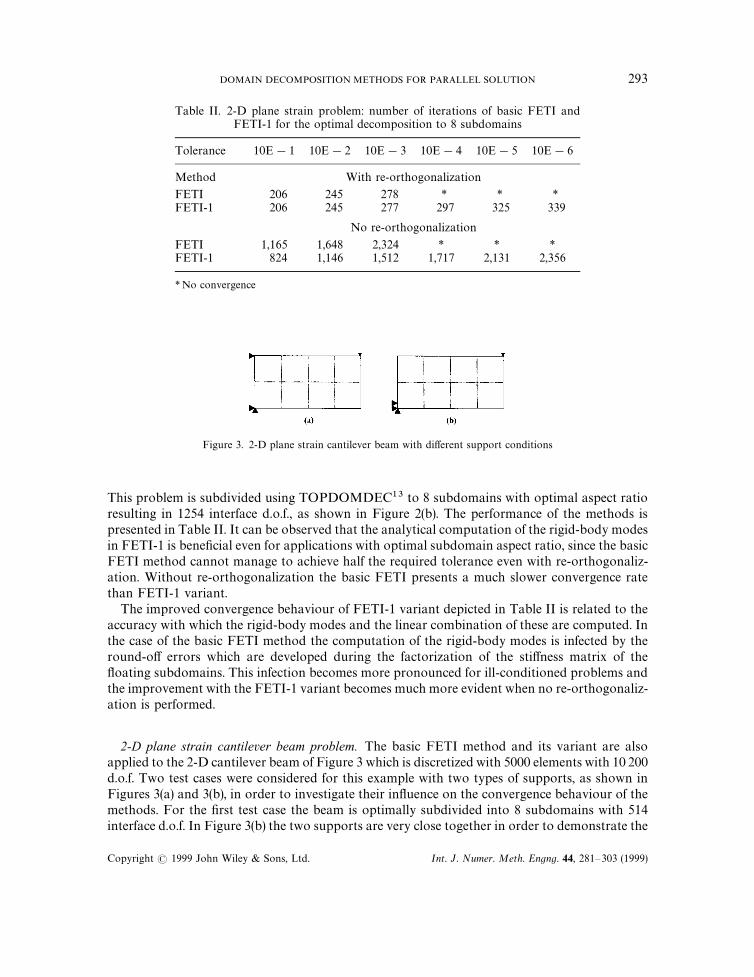
Table II. 2-D plane strain problem: number of iterations of basic FETI andFETI-1 for the optimal decomposition to 8 subdomains

Tolerance 10E!1 10E!2 10E!3 10E!4 10E!5 10E!6

Method With re-orthogonalization

FETI 206 245 278 * * *FETI-1 206 245 277 297 325 339

No re-orthogonalization

FETI 1,165 1,648 2,324 * * *FETI-1 824 1,146 1,512 1,717 2,131 2,356

*No convergence

Figure 3. 2-D plane strain cantilever beam with different support conditions

This problem is subdivided using TOPDOMDEC13 to 8 subdomains with optimal aspect ratioresulting in 1254 interface d.o.f., as shown in Figure 2(b). The performance of the methods ispresented in Table II. It can be observed that the analytical computation of the rigid-body modesin FETI-1 is beneficial even for applications with optimal subdomain aspect ratio, since the basicFETI method cannot manage to achieve half the required tolerance even with re-orthogonaliz-ation. Without re-orthogonalization the basic FETI presents a much slower convergence ratethan FETI-1 variant.

The improved convergence behaviour of FETI-1 variant depicted in Table II is related to theaccuracy with which the rigid-body modes and the linear combination of these are computed. Inthe case of the basic FETI method the computation of the rigid-body modes is infected by theround-off errors which are developed during the factorization of the stiffness matrix of thefloating subdomains. This infection becomes more pronounced for ill-conditioned problems andthe improvement with the FETI-1 variant becomes much more evident when no re-orthogonaliz-ation is performed.

2-D plane strain cantilever beam problem. The basic FETI method and its variant are alsoapplied to the 2-D cantilever beam of Figure 3 which is discretized with 5000 elements with 10 200d.o.f. Two test cases were considered for this example with two types of supports, as shown inFigures 3(a) and 3(b), in order to investigate their influence on the convergence behaviour of themethods. For the first test case the beam is optimally subdivided into 8 subdomains with 514interface d.o.f. In Figure 3(b) the two supports are very close together in order to demonstrate the



Table III. 2-D cantilever beam—Test case 1:number of iterations of basic FETI and FETI-1

Poissonratio 0)3 0)49 0)4999

Method distant supports

FETI 51 116 *FETI-1 51 116 231

close supports

FETI 57 * *FETI-1 57 118 240

*No convergence

Table IV. 2-D cantilever beam—Test case 2:number of iterations of basic FETI and FETI-1

Subdomains 2 4 8

Method l"0)4999

FETI * * 241FETI-1 60 116 240

l"0)499999

FETI * * 316FETI-1 65 172 314

*No convergence

effect of large rigid-body movements associated with small strains on the convergence behaviourof the FETI method. As can be seen in Table III the location of the supports affects theconvergence behaviour of the methods. Furthermore, the basic FETI method is much moresensitive to the position of the restraints since the influence of the infected rigid-body modes bythe round-off errors appears to be more decisive for badly restrained structures.

Table IV depicts the performance of the methods for the cantilever beam of Figure 4 fordifferent number of subdivisions. The results confirm the superiority of FETI-1 over the basicFETI method which is affected by the accuracy with which the rigid-body modes are computedduring the factorization of the subdomain stiffness matrices. This accuracy is reduced as the sizeof the subdomains become larger.

Shape optimization test examples

Two benchmark shape optimization test examples are used to demonstrate the efficiency of theproposed methods using the shape optimization code ADOPT.4 The first example is a long,slender domain which has a rather dense global stiffness matrix with narrow bandwidth, whereasthe global stiffness matrix of the second example has a sparse pattern with a relatively large



Figure 4. 2-D plane strain cantilever beam with different number of subdivisions

bandwidth. The performance of the proposed solution methods is investigated and compared firstin serial computing mode with the conventional direct skyline and PCG, NCG and Lanczossolvers proposed in Reference 2. NCG is a PCG algorithm in which the preconditioning step isperformed via a Neumann series expansion of the stiffness matrix. Furthermore, the parallelperformance of basic FETI method and its variants is investigated in both types of sensitivityanalysis problems, while the two-level PCG method is applied for the GFD sensitivity analysistest cases. The convergence tolerance for all solution methods was taken as 10~3. For these testexamples plane stress conditions and isotropic material properties were assumed (elastic modulusE"210 000 N/mm2 and Poisson’s ratio l"0)3).

The following abbreviations are used: Direct is the conventional skyline direct solver; PCG(t)and Lanczos(t) are the PCG and Lanczos solvers, respectively, with the preconditioning matrixproduced via a complete, or an incomplete Cholesky factorization controlled by the rejectionparameter t10. A value of t between 0 and 1 corresponds to an incomplete Cholesky precondi-tioner, while t"0 gives the complete factorized matrix. NCG-i is the NCG solver with i terms ofthe Neumann series expansion. Finally, the two variants of the two-level methodology, combinedwith the FETI-2 variant, namely the GSI(PCG)-FETI-2 and GSI(NCG)-FETI-2 methods, arecompared with the other solvers, both in serial and parallel computing modes, in the case of GFDsensitivity analysis problems.

Connecting rod problem.14 The problem definition is given in Figure 5. The linearly varyingline load between key points 4 and 6 has a maximum value of p"500 N/mm. The objective is tominimize the volume of the structure, subject to an equivalent stress limit of p

.!9"1200 N/mm2.

The design model, which makes use of symmetry, consists of 12 key points, 4 primary designvariables (7, 10, 11, 12) and 6 secondary design variables (7, 8, 9, 10, 11, 12). The stress constraintis imposed as a global constraint for all the Gauss points and as key point constraint for thekey points 2, 3, 4, 5, 6 and 12. The movement directions are indicated by the dashed arrows.Key points 8 and 9 are linked to 7 so that the shape of the arc is preserved throughoutthe optimization procedure. The problem is analysed with a fine mesh having 39 200 d.o.f.resulting in a dense global stiffness matrix with relatively narrow bandwidth. The characteristicd.o.f. for 4 and 8 subdomains, as depicted in Figure 6, are given in Table V. The ESA and the GFD



Figure 5. Connecting rod: (a) initial shape; (b) final shape

Figure 6. Connecting rod: subdivision in 4 and 8 subdomains

sensitivity analysis methods are used to compute the sensitivities with perturbation value*s"10~4.

Table VI demonstrates the performance of the methods operated in a sequential mode for thecase of ESA sensitivity analysis. In the basic FETI method and its variants the operations are



Table V. Connecting rod: characteristic d.o.f.for 4 and 8 subdomains

Subdomains 4 8

Total d.o.f. 39,200 39,200Internal d.o.f.* 10,038 5,118Interface d.o.f. 474 1,098

*Of the larger subdomain

Table VI. Connecting rod: performance ofthe methods in sequential mode with ESA

sensitivity analysis

Method(4 subdomains- Time Storage1 processor) (s) (Mbytes)

Direct skyline 186 47NCG-1 220 35Lanczos (1E!9) 209 16PCG (0) 205 34PCG (1E!9) 224 15FETI 257 14FETI-1 234 14FETI-2 198 8

Table VII. Connecting rod: performance of the methods in parallel mode withESA sensitivity analysis

Time StorageRight-handsides 1 2 3 4 5 (s) (Mbytes)

Method Iterations(4 processors)FETI 26 12 10 10 8 86 14FETI-2 26 12 10 10 8 69 8

Method Iterations(8 processors)FETI 36 16 15 13 11 59 9FETI-2 36 16 15 13 11 48 6

carried out in 4 subdomains. Following the results depicted in Table I it is expected that theperformance of the basic FETI method and its variants will be further improved for an increasednumber of subdomains. Table VII demonstrates the performance of the basic FETI method andFETI-2 variant, for the case of ESA sensitivity analysis, operated on parallel computing mode in



Table VIII. Connecting rod: performance of themethods in serial mode with GFD sensitivity analysis

Method(4 subdomains-1 processor)

Time(s)

Storage(Mbytes)

Direct skyline 844 47NCG-1 335 36PCG (0) 341 34PCG (1E!9) 374 15FETI 1,085 14FETI-2 823 8GSI(PCG)-FETI-2 368 9GSI(NCG)-FETI-2 360 10

Table IX. Connecting rod: performance of the methods in parallel mode with GFD sensitivity analysis

Right-hand time Storagesides 1 2 3 4 5 (s) (Mbytes)

Method (4 processors) Iterations

FETI 26 26 26 26 26 349 14FETI-2 26 26 26 26 26 264 8GSI(PCG)-FETI-2 26 14 12 10 9 8 8 7 6 124 9GSI(NCG)-FETI-2 26 14 12 10 9 8 8 7 6 122 10


FETI 36 36 36 36 36 247 9FETI-2 36 36 36 36 36 185 6GSI(PCG)-FETI-2 36 17 15 12 11 10 8 8 7 88 7GSI(NCG)-FETI-2 36 17 14 12 11 10 9 8 7 87 8

4 and 8 processors using 4 and 8 subdomains, respectively. Tables VIII and IX depict theperformance of the methods, for the case of GFD sensitivity analysis, operated on sequential andparallel computing modes, respectively. In Tables VII and IX the iteration history is also depictedfor five right-hand sides which correspond to the initial finite element solution and the sensitivityanalysis for the four design variables of the problem. In the case of the two level methods thenumber of iterations corresponds to the number of FETI iterations for the two global iterationsrequired for convergence.

Square plate problem with a central cut-out.14 The problem definition of this example is given inFigure 7 where, due to symmetry, only a quarter of the plate is modelled. The plate is underbiaxial tension with one side loaded with a distributed loading p"0)1538 N/mm2 and the otherside loaded only with half of this value, as shown in Figure 7. The objective is to minimize thevolume of the structure subject to an equivalent stress limit of p

.!9"7)0 N/mm2. The design

model consists of 8 key points and 5 primary design variables (2, 3, 4, 5, 6) which can move along



Figure 7. Square plate: (a) initial shape; (b) final shape

Figure 8. Square plate: subdivision in 4 and 8 subdomains

radial lines. The movement directions are indicated by the dashed arrows. The stress constraintsare imposed as a global constraint for all the Gauss points and as key point constraints for the keypoints 2, 3, 4, 5, 6 and 8. The problem is analysed with a fine mesh with 38 800 d.o.f. resulting ina sparse global stiffness matrix with relatively large bandwidth. The characteristic d.o.f. for 4 and8 subdomains, as depicted in Figure 8, are given in Table X. The ESA and the GFD methods areused to compute the sensitivities with *s"10~5.

Table XI demonstrates the performance of the methods operated in a sequential mode for thecase of ESA sensitivity analysis. In the basic FETI method and its variants the operations arecarried out in 4 subdomains. Table XII demonstrates the performance of the basic FETI method



Table X. Square plate: characteristic d.o.f. for4 and 8 subdomains

Subdomains 4 8

Total d.o.f. 38,800 38,800Internal d.o.f.* 9,738 5,122Interface d.o.f. 998 2,290

*Of the larger subdomain

Table XI. Square plate: performance of the methodsin sequential mode with ESA sensitivity analysis

Method(4 subdomains- Time Storage1 processor) (s) (Mbytes)

Direct skyline 502 95Lanczos (0) 524 63Lanczos (1E!9) 417 29PCG (0) 514 61PCG (1E!9) 425 27FETI 486 43FETI-1 466 43FETI-2 414 26

Table XII. Square plate: performance of the methods in parallel mode with ESAsensitivity analysis

Right-hand Time Storagesides 1 2 3 4 5 6 (s) (Mbytes)

method (4 processors) Iterations

FETI(no reorth) 67 60 65 51 53 53 420 41FETI 33 16 13 10 9 8 150 43FETI-2(no reorth) 67 60 65 51 53 53 306 24FETI-2 33 16 13 10 9 8 120 26

method (8 processors) Iterations

FETI(no reorth) 271 266 253 219 199 204 398 20FETI 64 24 18 14 11 11 92 23FETI-2(no reorth) 269 267 253 220 199 205 290 13FETI-2 64 24 18 14 11 11 70 16

and the FETI-2 variant, for the case of ESA sensitivity analysis, operated on parallel computingmode in 4 and 8 processors using 4 and 8 subdomains, respectively. The benefits from the use ofthe re-orthogonalization are also evident both in terms of PCPG iterations and computing time.Tables XIII and XIV depict the performance of the methods, for the case of GFD sensitivity



Table XIII. Square plate: performance of themethods in serial mode with GFD sensitivity

analysis

Method Time Storage(4 subdomains) (s) (Mbytes)

Direct skyline 2,790 95NCG-1 732 65PCG (0) 745 61PCG (1E!9) 714 27FETI 2,108 43FETI-2 1,782 26GSI(PCG)-FETI-2 795 27GSI(NCG)-FETI-2 779 29

Table XIV. Square plate: performance of the methods in parallel mode with GFD sensitivity analysis

Right-hand Time Storagesides 1 2 3 4 5 6 (s) (Mbytes)


FETI 33 33 33 33 33 33 667 43FETI-2 33 33 33 33 33 33 574 26GSI(PCG)-FETI-2 33 17 13 12 10 10 8 8 7 7 6 256 27GSI(NCG)-FETI-2 33 17 14 12 11 11 9 7 7 6 6 249 29


FETI 64 64 64 64 64 64 396 23FETI-2 64 64 64 64 64 64 332 16GSI(PCG)-FETI-2 64 24 19 17 14 12 11 9 9 8 7 165 17GSI(NCG)-FETI-2 64 24 18 16 14 13 11 10 9 8 7 163 18

analysis, operated on sequential and parallel computing modes, respectively. In Tables XII andXIV the iteration history is also depicted for six right-hand sides, which correspond to the initialfinite element solution and the sensitivity analysis for the five design variables of the problem. Inthe case of the two level methods the number of iterations corresponds to the number of FETIiterations for the two global iterations required for convergence.

DISCUSSION OF THE RESULTS AND CONCLUSIONS

The variant FETI-1, where the rigid-body modes are computed explicitly, increases the robust-ness of the basic FETI method for ill-conditioned problems. Although re-orthogonalizationameliorates this deficiency of the basic FETI method, it is still present in 3-D large-scale and/or2-D ill-conditioned problems, where the basic FETI method was found incapable to converge tostricter tolerances for a class of ill-conditioned problems. The second variant FETI-2, where thelocal problem is solved via the PCG algorithm, retains the characteristics of the first variant and



operates on reduced storage requirements which are particularly important when solving large-scale 3-D problems. The benefits from the reduced computer storage demands of the FETI-2variant are retained when more subdivisions are allocated at each processor since the beneficialeffect of solving local problems with smaller bandwidths is equally exploited by the basic FETImethod and by FETI-2 variant.

In the case of sensitivity analysis with the ‘exact’ semi-analytical approach, the two FETIvariants outperform the basic FETI method, both in sequential and in parallel computing modes,as well as the direct skyline solver, the global PCG and Lanczos methods in sequential computingmode. In the connecting rod problem with a small bandwidth, the direct skyline solver is slightlyfaster than the FETI-2 variant with re-orthogonalization, but requires 6 times more computerstorage. In the square plate problem with a relatively sparse stiffness matrix the FETI-2 methodwith re-orthogonalization is 1)25 times faster than the direct skyline solver and requires 6 timesless computer storage. For this example the global PCG and Lanczos methods with incompleteCholesky factorization preconditioners outperform the skyline solver, both in terms of computingtime and storage. In all cases the re-orthogonalization procedure proved to be extremelybeneficial to the performance of the domain decomposition methods.

In the case of sensitivity analysis with the global finite-difference approach, the superiority ofthe hybrid solution methods is more pronounced. The global PCG and Lanczos methods are 2)5and 4 times faster than the direct solver in the dense and sparse example, respectively, and reducestorage requirements by 65 per cent in both cases. The proposed two-level methods, namely theGSI(PCG)-FETI-2 and GSI(NCG)-FETI-2 (with two terms in the Neumann series expansion),appear to perform equally well, in the sequential mode, compared to the global PCG andLanczos methods with incomplete Cholesky factorization preconditioners, while they outperformthe direct skyline solver and the one-level FETI and its two variants by a factor ranging from 2.3to 3.5 for both examples. In the parallel computing mode the superiority of the two-level methodsis retained over the one-level domain decomposition methods by a factor of more than 2 in bothexamples considered. The benefits of using the FETI-2 variant instead of the basic FETI methodis even more pronounced in this case.

It has to be pointed out that the overall optimization time with the global finite-differencesensitivity analysis is drastically reduced using the parallel version of the proposed two-levelGSI(PCG)-FETI methods. More specifically, using the direct skyline solver, the optimizationtime with the ‘exact’ semi-analytical sensitivity analysis is 5 times faster than the correspondingtime required by the global finite-difference sensitivity analysis, whereas using the paralleltwo-level PCG methods this ratio is reduced to 2. It is anticipated that for large-scale three-dimensional problems and for more design variables the superiority of the proposed methodswill become even more evident. Therefore by using the two-level methods in a parallel com-puting environment, the performance of GFD sensitivity analysis can become competitive to theSA type of sensitivity analysis particularly in large-scale 3-D shape optimization problems.Bearing in mind the simplicity and ease of the implementation of the GFD compared to thatof the SA, the former approach could be a prospective alternative to other sensitivity analysisapproaches.

ACKNOWLEDGEMENTS

This work has been supported by HC & M/9203390 project of the European Union. The authorswish to thank E. Hinton and J. Sienz for providing the shape optimization code ADOPT4. The



authors are also grateful to D. Harbis for his assistance with the linear solution test examples thatare presented in this work.

REFERENCES

1. C. Farhat and F.-X. Roux, ‘A method of finite element tearing and interconnecting and its parallel solution algorithm’,Int. J. Numer Meth. Engng., 32, 1205—1227 (1991).

2. M. Papadrakakis, Y. Tsompanakis, E. Hinton and J. Sienz, ‘Advanced solution methods in topology optimizationand shape sensitivity analysis’, J. Engng. Comput., 13(5), 57—90 (1996).

3. M. Papadrakakis, ‘Domain decomposition techniques for computational structural mechanics’, in M. Papadrakakis(ed.), Parallel Solution Methods in Computational Mechanics, Wiley, New York, 1997, pp. 87—141.

4. J. Sienz, ‘Integrated structural modelling, adaptive analysis and shape optimization’, Ph.D. ¹hesis, Dept. of Civil Eng.,Univ. of Wales, Swansea, UK, 1994.

5. K. U. Bletzinger, S. Kimmich and E. Ramm, ‘Efficient modeling in shape optimal design’, Comput. Systems Engng.,2(5/6), 483—495 (1991).

6. N. Olhoff, J. Rasmussen and E. Lund, ‘Method of exact numerical differentiation for error estimation in finite elementbased semi-analytical shape sensitivity analyses’, Special Report No. 10, Institute of Mechanical Engineering, AalborgUniversity, Aalborg, DK, 1992.

7. M. Papadrakakis and S. Smerou, ‘A new implementation of the Lanczos method in linear problems’, Int. J. Numer.Meth. Engng., 29, 141—159 (1990).

8. C. Farhat and F.-X. Roux, ‘Implicit parallel processing in structural mechanics’, Comput. Mech. Adv., 2, 1—124 (1994).9. M. Papadrakakis and S. Bitzarakis, ‘A dual substructure method for solving large-scale problems on parallel

computers’, Report 95-1, Institute of Structural Analysis and Seismic Research, NTUA, Athens, Greece, 1995.10. N. Bitoulas and M. Papadrakakis, ‘An optimised computer implementation of the incomplete Cholesky factoriz-

ation’, Comput. Systems Engng., 5(3), 265—274 (1994).11. S. Bitzarakis, M. Papadrakakis and A. Kotsopoulos, ‘Parallel solution techniques in computational structural

mechanics’, Comput. Meth. Appl. Mech. Eng., 148, 75—104 (1997).12. C. Farhat, L. Crivelli and F.-X. Roux, ‘Extending substructure based iterative solvers to multiple load and repeated

analyses’, Comput. Meth. Appl. Mech. Engng., 195—209 (1994).13. M. Sharp and C. Farhat, ‘TOPDOMDEC—A totally object oriented program for visualisation, domain decomposi-

tion and parallel processing’, ºser’s Manual, PGSoft and University of Colorado, Boulder, USA, 1994.14. E. Hinton and J. Sienz, ‘Studies with a robust and reliable structural shape optimization tool’, in B. H. V. Topping

(ed.), Developments in Computational ¹echniques for Structural Engineering, CIVIL-COMP Press, Edinburgh, 1995,pp. 343—358.



domain decomposition methods for parallel

Documents