NBER WORKING PAPER SERIES

DOUBLE/DEBIASED MACHINE LEARNING FOR TREATMENT AND STRUCTURAL PARAMETERS

Victor ChernozhukovDenis Chetverikov

Mert DemirerEsther Duflo

Christian HansenWhitney NeweyJames Robins

Working Paper 23564http://www.nber.org/papers/w23564

NATIONAL BUREAU OF ECONOMIC RESEARCH1050 Massachusetts Avenue

Cambridge, MA 02138June 2017

We would like to acknowledge research support from the National Science Foundation. We also thank participants of the MIT Stochastics and Statistics seminar, the Kansas Econometrics conference, the Royal Economic Society Annual Conference, The Hannan Lecture at the Australasian Econometric Society meeting, The Econometric Theory lecture at the EC2 meetings 2016 in Toulouse, The CORE 50th Anniversary Conference, The Becker-Friedman Institute Conference on Machine Learning and Economics, The INET conferences at USC on Big Data, the World Congress of Probability and Statistics 2016, the Joint Statistical Meetings 2016, the New England Day of Statistics Conference, CEMMAP's Masterclass on Causal Machine Learning, and St. Gallen's summer school on “Big Data", for many useful comments and questions. We would like to thank Susan Athey, Peter Aronow, Jin Hahn, Guido Imbens, Mark van der Laan, and Matt Taddy for constructive comments. We thank Peter Aronow for pointing us to the literature on targeted learning on which, along with prior works of Neyman, Bickel, and the many other contributions to semiparametric learning theory, we build. The views expressed herein are those of the authors and do not necessarily reflect the views of the National Bureau of Economic Research.

NBER working papers are circulated for discussion and comment purposes. They have not been peer-reviewed or been subject to the review by the NBER Board of Directors that accompanies official NBER publications.

© 2017 by Victor Chernozhukov, Denis Chetverikov, Mert Demirer, Esther Duflo, Christian Hansen, Whitney Newey, and James Robins. All rights reserved. Short sections of text, not to exceed two paragraphs, may be quoted without explicit permission provided that full credit, including © notice, is given to the source.

Double/Debiased Machine Learning for Treatment and Structural Parameters Victor Chernozhukov, Denis Chetverikov, Mert Demirer, Esther Duflo, Christian Hansen, Whitney Newey, and James Robins NBER Working Paper No. 23564 June 2017 JEL No. C01

ABSTRACT

We revisit the classic semiparametric problem of inference on a low dimensional parameter θ0 in the presence of high-dimensional nuisance parameters η0. We depart from the classical setting by allowing for η0 to be so high-dimensional that the traditional assumptions, such as Donsker properties, that limit complexity of the parameter space for this object break down. To estimate η0, we consider the use of statistical or machine learning (ML) methods which are particularly well-suited to estimation in modern, very high-dimensional cases. ML methods perform well by employing regularization to reduce variance and trading off regularization bias with overfitting in practice. However, both regularization bias and overfitting in estimating η0 cause a heavy bias in estimators of θ0 that are obtained by naively plugging ML estimators of η0 into estimating equations for θ0. This bias results in the naive estimator failing to be N-1/2 consistent, where N is the sample size. We show that the impact of regularization bias and overfitting on estimation of the parameter of interest θ0 can be removed by using two simple, yet critical, ingredients: (1) using Neyman-orthogonal moments/scores that have reduced sensitivity with respect to nuisance parameters to estimate θ0, and (2) making use of cross-fitting which provides an efficient form of data-splitting. We call the resulting set of methods double or debiased ML (DML). We verify that DML delivers point estimators that concentrate in a N-1/2-neighborhood of the true parameter values and are approximately unbiased and normally distributed, which allows construction of valid confidence statements. The generic statistical theory of DML is elementary and simultaneously relies on only weak theoretical requirements which will admit the use of a broad array of modern ML methods for estimating the nuisance parameters such as random forests, lasso, ridge, deep neural nets, boosted trees, and various hybrids and ensembles of these methods. We illustrate the general theory by applying it to provide theoretical properties of DML applied to learn the main regression parameter in a partially linear regression model, DML applied to learn the coefficient on an endogenous variable in a partially linear instrumental variables model, DML applied to learn the average treatment effect and the average treatment effect on the treated under unconfoundedness, and DML applied to learn the local average treatment effect in an instrumental variables setting. In addition to these theoretical applications, we also illustrate the use of DML in three empirical examples.

Victor Chernozhukov Department of Economics Massachusetts Institute of Technology 77 Massachusetts Avenue Cambridge, Mass. 02139 vchern@mit.edu

Denis Chetverikov UCLA, Department of Economics 315 Portola Plaza Bunche Hall, Room 8283 Los Angeles, CA 90095-1477 chetverikov@econ.ucla.edu

Mert Demirer Department of Economics Massachusetts Institute of Technology 77 Massachusetts Avenue E52-300 Cambridge, MA 02139 mdemirer@mit.edu

Esther Duflo Department ofEconomics, E52-544 MIT 77 Massachusetts Avenue Cambridge, MA 02139 and NBER eduflo@mit.edu

Christian Hansen University of Chicago Booth School of Business 5807 South Woodlawn Avenue Chicago, IL 60637 chansen1@chicagobooth.edu

Whitney Newey Department of Economics Massachusetts Institute of Technology 77 Massachusetts Avenue Cambridge, MA 02139 wnewey@mit.edu

James Robins Harvard University T.H. Chan School of Public Health 677 Huntington Avenue Kresge Building Room 823 Boston, MA 02115 robins@hsph.harvard.edu

2 CCDDHNR

treatment effect in an instrumental variables setting. In addition to these theoreticalapplications, we also illustrate the use of DML in three empirical examples.

1. INTRODUCTION AND MOTIVATION

1.1. Motivation

We develop a series of simple results for obtaining root-N consistent estimation, where Nis the sample size, and valid inferential statements about a low-dimensional parameter ofinterest, θ0, in the presence of a high-dimensional or “highly complex” nuisance parame-ter, η0. The parameter of interest will typically be a causal parameter or treatment effectparameter, and we consider settings in which the nuisance parameter will be estimatedusing machine learning (ML) methods such as random forests, lasso or post-lasso, neu-ral nets, boosted regression trees, and various hybrids and ensembles of these methods.These ML methods are able to handle many covariates and provide natural estimatorsof nuisance parameters when these parameters are highly complex. Here, highly complexformally means that the entropy of the parameter space for the nuisance parameter isincreasing with the sample size in a way that moves us outside of the traditional frame-work considered in the classical semi-parametric literature where the complexity of thenuisance parameter space is taken to be sufficiently small. Offering a general and simpleprocedure for estimating and doing inference on θ0 that is formally valid in these highlycomplex settings is the main contribution of this paper.

Example 1.1. (Partially Linear Regression) As a lead example, consider the fol-lowing partially linear regression (PLR) model as in Robinson (1988):

Y = Dθ0 + g0(X) + U, E[U | X,D] = 0, (1.1)

D = m0(X) + V, E[V | X] = 0, (1.2)

where Y is the outcome variable, D is the policy/treatment variable of interest,1 vector

X = (X1, ..., Xp)

consists of other controls, and U and V are disturbances. The first equation is the mainequation, and θ0 is the main regression coefficient that we would like to infer. If Dis exogenous conditional on controls X, θ0 has the interpretation of the treatment ef-fect (TE) parameter or “lift” parameter in business applications. The second equationkeeps track of confounding, namely the dependence of the treatment variable on controls.This equation is not of interest per se but is important for characterizing and remov-ing regularization bias. The confounding factors X affect the policy variable D via thefunction m0(X) and the outcome variable via the function g0(X). In many applications,the dimension p of vector X is large relative to N . To capture the feature that p is notvanishingly small relative to the sample size, modern analyses then model p as increasing

1We consider the case where D is a scalar for simplicity. Extension to the case where D is a vectorof fixed, finite dimension is accomplished by introducing an equation like (1.2) for each element of thevector.

DML 3

with the sample size, which causes traditional assumptions that limit the complexity ofthe parameter space for the nuisance parameters η0 = (m0, g0) to fail.

Regularization Bias. A naive approach to estimation of θ0 using ML methods wouldbe, for example, to construct a sophisticated ML estimator Dθ0 + g0(X) for learning theregression function Dθ0 +g0(X).2 Suppose, for the sake of clarity, that we randomly splitthe sample into two parts: a main part of size n, with observation numbers indexed byi ∈ I, and an auxiliary part of size N − n, with observations indexed by i ∈ Ic. Forsimplicity, we take n = N/2 for the moment and turn to more general cases which coverunequal split-sizes, using more than one split, and achieving the same efficiency as if thefull sample were used for estimating θ0 in the formal development in Section 3. Supposeg0 is obtained using the auxiliary sample and that, given this g0, the final estimate of θ0

is obtained using the main sample:

θ0 =( 1

n

∑i∈I

D2i

)−1 1

n

∑i∈I

Di(Yi − g0(Xi)). (1.3)

The estimator θ0 will generally have a slower than 1/√n rate of convergence, namely,

|√n(θ0 − θ0)| →P ∞. (1.4)

As detailed below, the driving force behind this “inferior” behavior is the bias in learningg0. Figure 1 provides a numerical illustration of this phenomenon for a naive ML estimatorbased on a random forest in a simple computational experiment.

To heuristically illustrate the impact of the bias in learning g0, we can decompose thescaled estimation error in θ0 as

√n(θ0− θ0) =

( 1

n

∑i∈I

D2i

)−1 1√n

∑i∈I

DiUi︸ ︷︷ ︸:=a

+( 1

n

∑i∈I

D2i

)−1 1√n

∑i∈I

Di(g0(Xi)− g0(Xi))︸ ︷︷ ︸:=b

.

The first term is well-behaved under mild conditions, obeying a ; N(0, Σ) for some Σ.Term b is the regularization bias term, which is not centered and diverges in general.Indeed, we have

b = (EDi2)−1 1√

n

∑i∈I

m0(Xi)(g0(Xi)− g0(Xi)) + oP (1)

to the first order. Heuristically, b is the sum of n terms that do not have mean zero,m0(Xi)(g0(Xi) − g0(Xi)), divided by

√n. These terms have non-zero mean because,

in high dimensional or otherwise highly complex settings, we must employ regularizedestimators - such as lasso, ridge, boosting, or penalized neural nets - for informativelearning to be feasible. The regularization in these estimators keeps the variance of theestimator from exploding but also necessarily induces substantive biases in the estimatorg0 of g0. Specifically, the rate of convergence of (the bias of) g0 to g0 in the root meansquared error sense will typically be n−ϕg with ϕg < 1/2. Hence, we expect b to be ofstochastic order

√nn−ϕg → ∞ since Di is centered at m0(Xi) 6= 0, which then implies

(1.4).

2For instance, we could use lasso if we believe g0 is well-approximated by a sparse linear combination ofprespecified functions of X. In other settings, we could, for example, use iterative methods that alternatebetween random forests, for estimating g0, and least squares, for estimating θ0.

4 CCDDHNR

-0.2 -0.15 -0.1 -0.05 0 0.05 0.1 0.15 0.20

1

2

3

4

5

6

7

8

9

10

Non-Orthogonal, n = 500, p = 20

SimulationN(0,'

s)

-0.2 -0.15 -0.1 -0.05 0 0.05 0.1 0.15 0.20

1

2

3

4

5

6

7

8

9

10

Orthogonal, n = 500, p = 20

SimulationN(0,'

s)

1

Figure 1. Left Panel: Behavior of a conventional (non-orthogonal) ML estimator, θ0, in the partiallylinear model in a simple simulation experiment where we learn g0 using a random forest. The g0 in thisexperiment is a very smooth function of a small number of variables, so the experiment is seeminglyfavorable to the use of random forests a priori. The histogram shows the simulated distribution of the

centered estimator, θ0 − θ0. The estimator is badly biased, shifted much to the right relative to thetrue value θ0. The distribution of the estimator (approximated by the blue histogram) is substantivelydifferent from a normal approximation (shown by the red curve) derived under the assumption that the

bias is negligible. Right Panel: Behavior of the orthogonal, DML estimator, θ0, in the partially linearmodel in a simple experiment where we learn nuisance functions using random forests. Note that thesimulated data are exactly the same as those underlying left panel. The simulated distribution of thecentered estimator, θ0−θ0, (given by the blue histogram) illustrates that the estimator is approximatelyunbiased, concentrates around θ0, and is well-approximated by the normal approximation obtained inSection 3 (shown by the red curve).

Overcoming Regularization Biases using Orthogonalization. Now consider asecond construction that employs an “orthogonalized” formulation obtained by directlypartialling out the effect of X from D to obtain the orthogonalized regressor V = D −m0(X). Specifically, we obtain V = D − m0(X), where m0 is an ML estimator of m0

obtained using the auxiliary sample of observations. We are now solving an auxiliaryprediction problem to estimate the conditional mean of D given X, so we are doing“double prediction” or “double machine learning”.

After partialling the effect of X out from D and obtaining a preliminary estimate of g0

from the auxiliary sample as before, we may formulate the following “debiased” machinelearning estimator for θ0 using the main sample of observations:3

θ0 =( 1

n

∑i∈I

ViDi

)−1 1

n

∑i∈I

Vi(Yi − g0(Xi)). (1.5)

By approximately orthogonalizing D with respect to X and approximately removing thedirect effect of confounding by subtracting an estimate of g0, θ0 removes the effect of

3In Section 4, we also consider another debiased estimator, based on the partialling-out approach ofRobinson (1988):

θ0 =( 1

n

∑i∈I

ViVi

)−1 1

n

∑i∈I

Vi(Yi − 0(Xi)), `0(X) = E[Y |X].

DML 5

regularization bias that contaminates (1.3). The formulation of θ0 also provides directlinks to both the classical econometric literature, as the estimator can clearly be inter-preted as a linear instrumental variable (IV) estimator, and to the more recent literatureon debiased lasso in the context where g0 is taken to be well-approximated by a sparselinear combination of prespecified functions of X; see, e.g., Belloni et al. (2013); Zhangand Zhang (2014); Javanmard and Montanari (2014b); van de Geer et al. (2014); Belloniet al. (2014); and Belloni et al. (2014).4

To illustrate the benefits of the auxiliary prediction step and estimating θ0 with θ0,we sketch the properties of θ0 here. We can decompose the scaled estimation error of θ0

into three components:√n(θ0 − θ0) = a∗ + b∗ + c∗.

The leading term, a∗, will satisfy

a∗ = (EV 2)−1 1√n

∑i∈I

ViUi ; N(0,Σ)

under mild conditions. The second term, b∗, captures the impact of regularization biasin estimating g0 and m0. Specifically, we will have

b∗ = (EV 2)−1 1√n

∑i∈I

(m0(Xi)−m0(Xi))(g0(Xi)− g0(Xi)),

which now depends on the product of the estimation errors in m0 and g0. Because thisterm depends only on the product of the estimation errors, it can vanish under a broadrange of data-generating processes. Indeed, this term is upper-bounded by

√nn−(ϕm+ϕg),

where n−ϕm and n−ϕg are respectively the rates of convergence of m0 to m0 and g0 tog0; and this upper bound can clearly vanish even though both m0 and g0 are estimatedat relatively slow rates. Verifying that θ0 has good properties then requires that theremainder term, c∗, is sufficiently well-behaved. Sample-splitting will play a key role inallowing us to guarantee that c∗ = oP (1) under weak conditions as outlined below anddiscussed in detail in Section 3.

The Role of Sample Splitting in Removing Bias Induced by Overfitting.Our analysis makes use of sample-splitting which plays a key role in establishing thatremainder terms, like c∗, vanish in probability. In the partially linear model, we havethat the remainder c∗ contains terms like

1√n

∑i∈I

Vi(g0(Xi)− g0(Xi)) (1.6)

that involve 1/√n normalized sums of products of structural unobservables from model

(1.1)-(1.2) with estimation errors in learning the nuisance functions g0 and m0 and needto be shown to vanish in probability. The use of sample splitting allows simple and tightcontrol of such terms. To see this, assume that observations are independent and recallthat g0 is estimated using only observations in the auxiliary sample. Then, conditioningon the auxiliary sample and recalling that E[Vi|Xi] = 0, it is easy to verify that term

4Each of these works differs in terms of detail but can be viewed through the lens of either “debiasing” or“orthogonalization” to alleviate the impact of regularization bias on subsequent estimation and inference.

6 CCDDHNR

(1.6) has mean zero and variance of order

1

n

∑i∈I

(g0(Xi)− g0(Xi))2 →P 0.

Thus, the term (1.6) vanishes in probability by Chebyshev’s inequality.While sample splitting allows us to deal with remainder terms such as c∗, its direct

application does have the drawback that the estimator of the parameter of interest onlymakes use of the main sample which may result in a substantial loss of efficiency as weare only making use of a subset of the available data. However, we can flip the role of themain and auxiliary samples to obtain a second version of the estimator of the parameterof interest. By averaging the two resulting estimators, we may regain full efficiency.Indeed, the two estimators will be approximately independent, so simply averaging themoffers an efficient procedure. We call this sample splitting procedure where we swap theroles of main and auxiliary samples to obtain multiple estimates and then average theresults cross-fitting. We formally define this procedure and discuss a K-fold version ofcross-fitting in Section 3.

Without sample splitting, terms such as (1.6) may not vanish and can lead to poorperformance of estimators of θ0. The difficulty arises because model errors, such as Vi,and estimation errors, such as g0(Xi) − g0(Xi), are generally related because the datafor observation i is used in forming the estimator g0. The association may then lead topoor performance of an estimator of θ0 that makes use of g0 as a plug-in estimator forg0 even when this estimator converges at a very favorable rate, say N−1/2+ε.

As an artificial but illustrative example of the problems that may result from overfit-ting, let g0(Xi) = g0(Xi) + (Yi − g0(Xi))/N

1/2−ε for any i in the sample used to formestimator g0, and note that the second term provides a simple model that captures over-fitting of the outcome variable within the estimation sample. This estimator is excellentin terms of rates: If the Ui’s and Di’s are bounded, g0 converges uniformly to g0 atthe nearly parametric rate N−1/2+ε. Despite this fast rate of convergence, term c∗ nowexplodes if we do not use sample splitting. For example, suppose that the full sample isused to estimate both g0 and θ0. A simple calculation then reveals that term c∗ becomes

1√N

N∑i=1

Vi(g0(Xi)− g0(Xi)) ∝ N ε →∞.

This bias due to overfitting is illustrated in the left panel of Figure 2. The histogramin the figure gives a simulated distribution for the studentized θ resulting from using thefull sample and the contrived estimator g(Xi) given above. We can see that the histogramis shifted markedly to the left demonstrating substantial bias resulting from overfitting.The right panel of Figure 2 also illustrates that this bias is completely removed bysample splitting. The results the right panel of Figure 2 make use of the two-fold cross-fitting procedure discussed above using the estimator θ and the contrived estimator g(Xi)exactly as in the right panel. The difference is that g(Xi) is formed in one half of thesample and then θ is estimated using the other half of the sample. This procedure is thenrepeated swapping the roles of the two samples and the results are averaged. We cansee that the substantial bias from the full sample estimator has been removed and thatthe spread of the histogram corresponding to the cross-fit estimator is roughly the sameas that of the full sample estimator clearly illustrating the bias-reduction property andefficiency of the cross-fitting procedure.

DML 7

Figure 2. This figure illustrates how the bias resulting from overfitting in the estimation of nuisancefunctions can cause the main estimator θ0 to be biased and how sample splitting completely eliminatesthis problem. Left Panel: The histogram shows the finite-sample distribution of θ0 in the partiallylinear model where nuisance parameters are estimated with overfitting using the full sample, i.e. withoutsample splitting. The finite-sample distribution is clearly shifted to the left of the true parameter valuedemonstrating the substantial bias. Right Panel: The histogram shows the finite-sample distributionof θ0 in the partially linear model where nuisance parameters are estimated with overfitting using thecross-fitting sample-splitting estimator. Here, we see that the use of sample-splitting has completelyeliminated the bias induced by overfitting.

A less contrived example that highlights the improvements brought by sample-splittingis the sparse high-dimensional instrumental variable (IV) model analyzed in Belloni et al.(2012). Specifically, they consider the IV model

Y = Dθ0 + ε

where E[ε|D] 6= 0 but instruments Z exist such that E[D|Z] is not a constant andE[ε|Z] = 0. Within this model, Belloni et al. (2012) focus on the problem of estimating theoptimal instrument, η0(Z) = E[D|Z] using lasso-type methods. If η0(Z) is approximatelysparse in the sense that only s terms of the dictionary of series transformations B(Z) =(B1(Z), . . . , Bp(Z)) are needed to approximate the function accurately, Belloni et al.(2012) require that s2 n to establish their asymptotic results when sample splitting isnot used but show that these results continue to hold under the much weaker requirementthat s n if one employs sample splitting. We note that this example provides aprototypical example where Neyman orthogonality holds and ML methods can usefullybe adopted to aid in learning structural parameters of interest. We also note that theweaker conditions required when using sample sample-splitting would also carry over tosparsity-based estimators in the partially linear model cited above. We discuss this inmore detail in Section 4.

While we find substantial appeal in using sample-splitting, one may also use empiricalprocess methods to verify that biases introduced due to overfitting are negligible. Forexample, consider the problematic term in the partially linear model described previously,

1√n

∑i∈I Vi(g0(Xi)− g0(Xi)). This term is clearly bounded by

supg∈GN

∣∣∣ 1√n

∑i∈I

Vi(g(Xi)− g0(Xi))∣∣∣, (1.7)

where GN is the smallest class of functions that contains estimators of g0, g, with high

8 CCDDHNR

probability. In conventional semiparametric statistical and econometric analysis, the com-plexity of GN is controlled by invoking Donsker conditions which allow verification thatterms such as (1.7) vanish asymptotically. Importantly, Donsker conditions require thatGN has bounded complexity, specifically a bounded entropy integral. Because of the latterproperty, Donsker conditions are inappropriate in settings using ML methods where thedimension of X is modeled as increasing with the sample size and estimators necessarilylive in highly complex spaces. For example, Donsker conditions rule out even the simplestlinear parametric model with high-dimensional regressors with parameter space given bythe Euclidean ball with the unit radius:

GN = x 7→ g(x) = x′θ; θ ∈ RpN : ‖θ‖ 6 1.

The entropy of this model, as measured by the logarithm of the covering number, growsat the rate pN . Without invoking Donsker conditions, one may still show that termssuch as (1.7) vanish as long as GN ’s entropy does not increase with N too rapidly. Afairly general treatment is given in Belloni et al. (2013) who provide a set of conditionsunder which terms like c∗ can vanish making use of the full sample. However, theseconditions on the growth of entropy could result in unnecessarily strong restrictions onmodel complexity, such as very strict requirements on sparsity in the context of lassoestimation as demonstrated in IV example mentioned above. Sample splitting allows oneto obtain good results under very weak conditions.

Neyman Orthogonality and Moment Conditions. Now we turn to a generaliza-tion of the orthogonalization principle above. The first “conventional” estimator θ0 givenin (1.3) can be viewed as a solution to estimating equations

1

n

∑i∈I

ϕ(W ; θ0, g0) = 0,

where ϕ is a known “score” function and g0 is the estimator of the nuisance parameterg0. For example, in the partially linear model above, the score function is ϕ(W ; θ, g) =(Y − θD − g(X))D. It is easy to see that this score function ϕ is sensitive to biasedestimation of g. Specifically, the Gateaux derivative operator5 with respect to g does notvanish:

∂gEϕ(W ; θ0, g0)[g − g0] 6= 0.

The proofs of the general results in Section 3 show that this term’s vanishing is a key toestablishing good behavior of an estimator for θ0.

By contrast the orthogonalized or double/debiased ML estimator θ0 given in (1.5)solves

1

n

∑i∈I

ψ(W ; θ0, η0) = 0,

where η0 is the estimator of the nuisance parameter η0 and ψ is an orthogonalized ordebiased “score” function that satisfies the property that the Gateaux derivative operatorwith respect to η vanishes when evaluated at the true parameter values:

∂ηEψ(W ; θ0, η0)[η − η0] = 0. (1.8)

We refer to property (1.8) as “Neyman orthogonality” and to ψ as the Neyman orthogonal

5See Section 2 for the definition of the Gateaux derivative operator.

DML 9

score function due to the fundamental contributions in Neyman (1959) and Neyman(1979), where this notion was introduced. Intuitively, the Neyman orthogonality conditionmeans that the moment conditions used to identify θ0 are locally insensitive to the valueof the nuisance parameter which allows one to plug-in noisy estimates of these parameterswithout strongly violating the moment condition. In the partially linear model (1.1)-(1.2),the estimator θ0 uses the score function ψ(W ; θ, η) = (Y −Dα−g(X))(D−m(X)), withthe nuisance parameter being η = (m, g). It is easy to see that these score functions ψ arenot sensitive to biased estimation of η0 in the sense that (1.8) holds. The proofs of thegeneral results in Section 3 show that this property and sample splitting are two generickeys that allow establishing good behavior of an estimator for θ0.

1.2. Literature Overview

Our paper builds upon two important bodies of research within the semiparametric liter-ature. The first is the literature on obtaining

√N -consistent and asymptotically normal

estimates of low-dimensional objects in the presence of high-dimensional or nonparamet-ric nuisance functions. The second is the literature on the use of sample-splitting to relaxentropy conditions. We provide links to each of these literatures in turn.

The problem we study is obviously related to the classical semiparametric estimationframework which focuses on obtaining

√N -consistent and asymptotically normal esti-

mates for low-dimensional components with nuisance parameters estimated by conven-tional nonparametric estimators such as kernels or series. See, for example, the work byLevit (1975), Ibragimov and Hasminskii (1981), Bickel (1982), Robinson (1988), Newey(1990), van der Vaart (1991), Andrews (1994a), Newey (1994), Newey et al. (1998),Robins and Rotnitzky (1995), Linton (1996), Bickel et al. (1998), Chen et al. (2003),Newey et al. (2004), van der Laan and Rose (2011), and Ai and Chen (2012). Neymanorthogonality (1.8), introduced by Neyman (1959), plays a key role in optimal testingtheory and adaptive estimation, semiparametric learning theory and econometrics, and,more recently, targeted learning theory. For example, Andrews (1994a), Newey (1994) andvan der Vaart (1998) provide a general set of results on estimation of a low-dimensionalparameter θ0 in the presence of nuisance parameters η0. Andrews (1994a) uses Ney-man orthogonality (1.8) and Donsker conditions to demonstrate the key equicontinuitycondition

1√n

∑i∈I

(ψ(Wi; θ0, η)−

∫ψ(w; θ0, η)dP (w)− ψ(Wi; θ0, η0)

)→P 0,

which reduces to (1.6) in the partially linear regression model. Newey (1994) gives condi-tions on estimating equations and nuisance function estimators so that nuisance functionestimators do not affect the limiting distribution of parameters of interest, providing asemiparametric version of Neyman orthogonality. van der Vaart (1998) discusses use ofsemiparametrically efficient scores to define estimators that solve estimating equationssetting averages of efficient scores to zero. He also uses efficient scores to define k-stepestimators, where a preliminary estimator is used to estimate the efficient score and thenupdating is done to further improve estimation; see also comments below on the use ofsample-splitting.

There is also a related targeted maximum likelihood learning approach, introduced inScharfstein et al. (1999) in the context of treatments effects analysis and substantiallygeneralized by van der Laan and Rubin (2006). van der Laan and Rubin (2006) use max-

10 CCDDHNR

imum likelihood in a least favorable direction and then perform “one-step” or “k-step”updates using the estimated scores in an effort to better estimate the target parameter.6

This procedure is like the least favorable direction approach in semiparametrics; see, forexample, Severini and Wong (1992). The introduction of the likelihood introduces majorbenefits such as allowing simple and natural imposition of constraints inherent in thedata, such as support restrictions when the outcome is binary or censored, and permit-ting the use of likelihood cross-validation to choose the nuisance parameter estimator.This data adaptive choice of the nuisance parameter has been dubbed the “super learner”by van der Laan et al. (2007). In subsequent work, van der Laan and Rose (2011) empha-size the use of ML methods to estimate the nuisance parameters for use with the superlearner. Much of this work, including recent work such as Luedtke and van der Laan(2016), Toth and van der Laan (2016), and Zheng et al. (2016), focuses on formal resultsunder a Donsker condition, though the use of sample splitting to relax these conditionshas also been advocated in the targeted maximum likelihood setting as discussed below.

The Donsker condition is a powerful classical condition that allows rich structures forfixed function classes G, but it is unfortunately unsuitable for high-dimensional settings.Examples of function classes where a Donsker condition holds include functions of asingle variable that have total variation bounded by 1 and functions x 7→ f(x) that haver > dim(x)/2 uniformly bounded derivatives. As a further example, functions composedfrom function classes with VC dimensions bounded by p through a fixed number ofalgebraic and monotone transforms are Donsker. However, this property will no longerhold if we let dim(x) grow to infinity with the sample size as this increase in dimensionwould require that the VC dimension also increases with n. More generally, Donskerconditions are easily violated once dimensions get large. A major point of departureof the present work from the classical literature on semiparametric estimation is itsexplicit focus on high-complexity/entropy cases. One way to analyze the problem ofestimation in high-entropy cases is to see to what degree equicontinuity results continueto hold while allowing moderate growth of the complexity/entropy of GN . Examples ofpapers taking this approach in an approximately sparse settings are Belloni et al. (2013),Belloni et al. (2014), Belloni et al. (2013), Chernozhukov et al. (2015b), Javanmardand Montanari (2014a), van de Geer et al. (2014), and Zhang and Zhang (2014). Inall of these examples, entropy growth must be limited in what may be very restrictiveways. The entropy conditions rule out the contrived overfitting example mentioned above,which does approximate realistic examples, and may otherwise place severe restrictionson the model. For example, in Belloni et al. (2010) and Belloni et al. (2012), the optimalinstrument needs to be sparse of order s

√n.

A key device that we use to avoid strong entropy conditions is cross-fitting via samplesplitting. Cross-fitting is a practical, efficient form of data splitting. Importantly, its usehere is not simply as a device to make proofs elementary (which it does), but as a prac-tical method to allow us to overcome the overfitting/high-complexity phenomena thatcommonly arise in data analysis based on highly adaptive ML methods. Our treatmentbuilds upon the sample-splitting ideas employed in Belloni et al. (2010) and Belloni et al.(2012) who considered sample-splitting in a high-dimensional sparse optimal IV model toweaken the sparsity condition mentioned in the previous paragraph to s n. This workin turn was inspired by Angrist and Krueger (1995). We also build on Ayyagari (2010)

6Targeted minimum loss estimation, which shares similar properties, is also discussed in e.g. van derLaan and Rose (2011) and van der Laan (2015).

DML 11

and Robins et al. (2013), where ML methods and sample splitting were used in the esti-mation of a partially linear model of the effects of pollution while controlling for severalcovariates. We use the term “cross-fitting” to characterize our recommended procedure,partly borrowing the jargon from Fan et al. (2012) which employed a slightly differentform of sample-splitting to estimate the scale parameter in a high-dimensional sparseregression. Of course, the use of sample-splitting to relax entropy conditions has a longhistory in semiparametric estimation problems. For example, Bickel (1982) consideredestimating nuisance functions using a vanishing fraction of the sample, and these resultswere extended to sample splitting into two equal halves and discretization of the param-eter space by Schick (1986). Similarly, van der Vaart (1998) uses 2-way sample splittingand discretization of the parameter space to give weak conditions for k-step estimatorsusing the efficient scores where sample splitting is used to estimate the “updates”; seealso Hubbard et al. (2016). Robins et al. (2008) and Robins et al. (2017) use samplesplitting in the construction of higher-order influence function corrections in semipara-metric estimation. Some recent work in the targeted maximum likelihood literature, forexample Zheng and van der Laan (2011), also notes the utility of sample splitting in thecontext of k-step updating, though this sample splitting approach is different from thecross-fitting approach we pursue.

Plan of the Paper. We organize the rest of the paper as follows. In Section 2, weformally define Neyman orthogonality and provide a brief discussion that synthesizesvarious models and frameworks that may be used to produce estimating equations sat-isfying this key condition. In Section 3, we carefully define DML estimators and developtheir general theory. We then illustrate this general theory by applying it to providetheoretical results for using DML to estimate and do inference for key parameters in thepartially linear regression model and for using DML to estimate and do inference forcoefficients on endogenous variables in a partially linear instrumental variables modelin Section 4. In Section 5, we provide a further illustration of the general theory byapplying it to develop theoretical results for DML estimation and inference for averagetreatment effects and average treatment effects on the treated under unconfoundednessand for DML estimation of local average treatment effects in an IV context within thepotential outcomes framework; see Imbens and Rubin (2015). Finally, we apply DML inthree empirical illustrations in Section 6. In an appendix, we define additional notationand present proofs.

Notation. The symbols P and E denote probability and expectation operators withrespect to a generic probability measure that describes the law of the data. If we need tosignify the dependence on a probability measure P , we use P as a subscript in PP and EP .We use capital letters, such as W , to denote random elements and use the correspondinglower case letters, such as w, to denote fixed values that these random elements cantake. In what follows, we use ‖ · ‖P,q to denote the Lq(P ) norm; for example, we denote

‖f‖P,q := ‖f(W )‖P,q :=(∫|f(w)|qdP (w)

)1/q. We use x′ to denote the transpose of a

column vector x. For a differentiable map x 7→ f(x), mapping Rd to Rk, we use ∂x′f toabbreviate the partial derivatives (∂/∂x′)f , and we correspondingly use the expression∂x′f(x0) to mean ∂x′f(x) |x=x0 , etc.

12 CCDDHNR

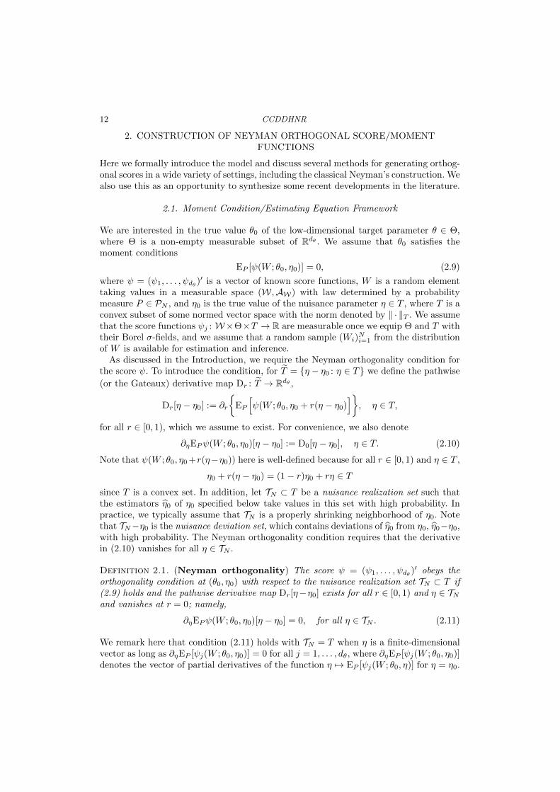
2. CONSTRUCTION OF NEYMAN ORTHOGONAL SCORE/MOMENTFUNCTIONS

Here we formally introduce the model and discuss several methods for generating orthog-onal scores in a wide variety of settings, including the classical Neyman’s construction. Wealso use this as an opportunity to synthesize some recent developments in the literature.

2.1. Moment Condition/Estimating Equation Framework

We are interested in the true value θ0 of the low-dimensional target parameter θ ∈ Θ,where Θ is a non-empty measurable subset of Rdθ . We assume that θ0 satisfies themoment conditions

EP [ψ(W ; θ0, η0)] = 0, (2.9)

where ψ = (ψ1, . . . , ψdθ )′ is a vector of known score functions, W is a random element

taking values in a measurable space (W,AW) with law determined by a probabilitymeasure P ∈ PN , and η0 is the true value of the nuisance parameter η ∈ T , where T is aconvex subset of some normed vector space with the norm denoted by ‖ · ‖T . We assumethat the score functions ψj : W×Θ×T → R are measurable once we equip Θ and T withtheir Borel σ-fields, and we assume that a random sample (Wi)

Ni=1 from the distribution

of W is available for estimation and inference.As discussed in the Introduction, we require the Neyman orthogonality condition for

the score ψ. To introduce the condition, for T = η − η0 : η ∈ T we define the pathwise

(or the Gateaux) derivative map Dr : T → Rdθ ,

Dr[η − η0] := ∂r

EP

[ψ(W ; θ0, η0 + r(η − η0)

], η ∈ T,

for all r ∈ [0, 1), which we assume to exist. For convenience, we also denote

∂ηEPψ(W ; θ0, η0)[η − η0] := D0[η − η0], η ∈ T. (2.10)

Note that ψ(W ; θ0, η0 +r(η−η0)) here is well-defined because for all r ∈ [0, 1) and η ∈ T ,

η0 + r(η − η0) = (1− r)η0 + rη ∈ T

since T is a convex set. In addition, let TN ⊂ T be a nuisance realization set such thatthe estimators η0 of η0 specified below take values in this set with high probability. Inpractice, we typically assume that TN is a properly shrinking neighborhood of η0. Notethat TN−η0 is the nuisance deviation set, which contains deviations of η0 from η0, η0−η0,with high probability. The Neyman orthogonality condition requires that the derivativein (2.10) vanishes for all η ∈ TN .

Definition 2.1. (Neyman orthogonality) The score ψ = (ψ1, . . . , ψdθ )′ obeys the

orthogonality condition at (θ0, η0) with respect to the nuisance realization set TN ⊂ T if(2.9) holds and the pathwise derivative map Dr[η−η0] exists for all r ∈ [0, 1) and η ∈ TNand vanishes at r = 0; namely,

∂ηEPψ(W ; θ0, η0)[η − η0] = 0, for all η ∈ TN . (2.11)

We remark here that condition (2.11) holds with TN = T when η is a finite-dimensionalvector as long as ∂ηEP [ψj(W ; θ0, η0)] = 0 for all j = 1, . . . , dθ, where ∂ηEP [ψj(W ; θ0, η0)]denotes the vector of partial derivatives of the function η 7→ EP [ψj(W ; θ0, η)] for η = η0.

DML 13

Sometimes it will also be helpful to use an approximate Neyman orthogonality condi-tion as opposed to the exact one given in Definition 2.1:

Definition 2.2. (Neyman Near-Orthogonality) The score ψ = (ψ1, . . . , ψdθ )′ obeys

the λN near-orthogonality condition at (θ0, η0) with respect to the nuisance realization setTN ⊂ T if (2.9) holds and the pathwise derivative map Dr[η − η0] exists for all r ∈ [0, 1)and η ∈ TN and is small at r = 0; namely,∥∥∥∂ηEPψ(W ; θ0, η0)[η − η0]

∥∥∥ 6 λN , for all η ∈ TN , (2.12)

where λNN>1 is a sequence of positive constants such that λN = o(N−1/2).

2.2. Construction of Neyman Orthogonal Scores

If we start with a score ϕ that does not satisfy the orthogonality condition above, wefirst transform it into a score ψ that does. Here we outline several methods for doing so.

2.2.1. Neyman Orthogonal Scores for Likelihood and Other M-Estimation Problems withFinite-Dimensional Nuisance Parameters

First, we describe the construction used by Neyman (1959) to derive his celebratedorthogonal score and C(α)-statistic in a maximum likelihood setting.7 Such constructionalso underlies the concept of local unbiasedness in construction of optimal tests in e.g.Ferguson (1967) and was extended to non-likelihood settings by Wooldridge (1991). Thediscussion of Neyman’s construction here draws on Chernozhukov et al. (2015a).

To describe the construction, let θ ∈ Θ ⊂ Rdθ and β ∈ B ⊂ Rdβ , where B is a convexset, be the target and the nuisance parameters, respectively. Further, suppose that thetrue parameter values θ0 and β0 solve the optimization problem

maxθ∈Θ, β∈B

EP [`(W ; θ, β)], (2.13)

where `(W ; θ, β) is a known criterion function. For example, `(W ; θ, β) can be the log-likelihood function associated to observation W . More generally, we refer to `(W ; θ, β)as the quasi-log-likelihood function. Then, under mild regularity conditions, θ0 and β0

satisfy

EP [∂θ`(W ; θ0, β0)] = 0, EP [∂β`(W ; θ0, β0)] = 0. (2.14)

Note that the original score function ϕ(W ; θ, β) = ∂θ`(W ; θ, β) for estimating θ0 willnot generally satisfy the orthogonality condition. Now consider the new score function,which we refer to as the Neyman orthogonal score,

ψ(W ; θ, η) = ∂θ`(W ; θ, β)− µ∂β`(W ; θ, β), (2.15)

where the nuisance parameter is

η = (β′, vec(µ)′)′ ∈ T = B × Rdθdβ ⊂ Rp, p = dβ + dθdβ ,

and µ is the dθ × dβ orthogonalization parameter matrix whose true value µ0 solves the

7The C(α)-statistic, or the orthogonal score statistic, has been explicitly used for testing and estimationin high-dimensional sparse models in Belloni et al. (2015).

14 CCDDHNR

equation

Jθβ − µJββ = 0 (2.16)

for

J =

(Jθθ JθβJβθ Jββ

)= ∂(θ′,β′)EP

[∂(θ′,β′)′`(W ; θ, β)

]∣∣∣θ=θ0; β=β0

.

The true value of the nuisance parameter η is

η0 = (β′0, vec(µ0)′)′; (2.17)

and when Jββ is invertible, (2.16) has the unique solution,

µ0 = JθβJ−1ββ . (2.18)

The following lemma shows that the score ψ in (2.15) satisfies the Neyman orthogonalitycondition.

Lemma 2.1. (Neyman Orthogonal Scores for Quasi-Likelihood Settings) If (2.14)holds, J exists, and Jββ is invertible, the score ψ in (2.15) is Neyman orthogonal at(θ0, η0) with respect to the nuisance realization set TN = T .

Proof. As discussed above, since J exists and Jββ is invertible, (2.16) has the uniquesolution µ0 given in (2.18), and so we have by (2.14) that E[ψ(W ; θ0, η0)] = 0 for η0 givenin (2.17). Moreover,

∂η′EPψ(W ; θ0, η0) =(

[Jθβ − µ0Jββ ],E[∂β′`(W ; θ0, β0)]⊗ Idθ×dθ)

= 0,

where Idθ×dθ is the dθ × dθ identity matrix and ⊗ is the Kronecker product. Hence, theasserted claim holds by the remark after Definition 2.1.

Remark 2.1. (Additional nuisance parameters) Note that the orthogonal score ψ in(2.15) has nuisance parameters consisting of the elements of µ in addition to the ele-ments of β, and Lemma 2.1 shows that Neyman orthogonality holds both with respect toβ and with respect to µ. We will find that Neyman orthogonal scores in other settings,including infinite-dimensional ones, have a similar property.

Remark 2.2. (Efficiency) Note that in this example, µ0 not only creates the necessaryorthogonality but also creates the efficient score for inference on the target parameter θwhen the quasi-log-likelihood function is the true (possibly conditional) log-likelihood, asdemonstrated by Neyman (1959).

Example 2.1. (High-Dimensional Linear Regression) As an application of the con-struction above, consider the following linear predictive model:

Y = Dθ0 +X ′β0 + U, EP [U(X ′, D)′] = 0, (2.19)

D = X ′γ0 + V, EP [V X] = 0, (2.20)

where for simplicity we assume that θ0 is a scalar. The first equation here is the mainpredictive model, and the second equation only plays a role in the construction of theNeyman orthogonal scores. It is well-known that θ0 and β0 in this model solve the opti-

DML 15

mization problem (2.13) with

`(W ; θ, β) = − (Y −Dθ −X ′β)2

2, θ ∈ Θ = R, β ∈ B = Rdβ ,

where we denoted W = (Y,D,X ′)′. Hence, equations (2.14) hold with

∂`θ(W ; θ, β) = (Y −Dθ −X ′β)D, ∂`β(W ; θ, β) = (Y −Dθ −X ′β)X,

and the matrix J satisfies

Jθβ = −EP [DX ′], Jββ = −EP [XX ′].

The Neyman orthogonal score is then given by

ψ(W ; θ, η) = (Y −Dθ −X ′β)(D − µX); η = (β′, vec(µ)′)′;

ψ(W ; θ0, η0) = U(D − µ0X); µ0 = EP [DX ′](EP [XX ′])−1 = γ′0. (2.21)

If the vector of covariates X here is high-dimensional but the vectors of parameters β0

and γ0 are approximately sparse, we can use `1-penalized least squares, `2-boosting, orforward selection methods to estimate β0 and γ0 = µ′0, and hence µ0 = (β′0, vec(µ0)′)′;see references cited in the Introduction.

If Jββ is not invertible, equation (2.16) typically has multiple solutions. In this case,it is convenient to focus on a minimal norm solution,

µ0 = arg min ‖µ‖ such that ‖Jθβ − µJββ‖q = 0

for a suitably chosen norm ‖ · ‖q on the space of dθ×dβ matrices. With an eye on solvingthe empirical version of this problem, we may also consider the relaxed version of thisproblem,

µ0 = arg min ‖µ‖ such that ‖Jθβ − µJββ‖q 6 rN (2.22)

for some rN > 0 such that rN → 0 as N →∞. This relaxation is also helpful when Jββ isinvertible but ill-conditioned. The following lemma shows that using µ0 in (2.22) leads toNeyman near-orthogonal scores. The proof of this lemma can be found in the Appendix.

Lemma 2.2. (Neyman Near-Orthogonal Scores for Quasi-Likelihood Settings)If (2.14) holds, J exists, the solution of the optimization problem (2.22) exists, and µ0 istaken to be this solution, the score ψ defined in (2.15) is Neyman λN near-orthogonal at(θ0, η0) with respect to the nuisance realization set TN = β ∈ B : ‖β−β0‖∗q 6 λN/rN×Rdθdβ , where the norm ‖ · ‖∗q on Rdβ is defined by ‖β‖∗q = supA ‖Aβ‖ with the supremumbeing taken over all dθ × dβ matrices A such that ‖A‖q 6 1.

Example 2.1. (High-Dimensional Linear Regression, Continued) In the high-dimensional linear regression example above, the relaxation (2.22) is helpful when Jββ =EP [XX ′] is ill-conditioned. Specifically, if one suspects that EP [XX ′] is ill-conditioned,one can define µ0 as the solution to the following optimization problem:

min ‖µ‖ such that ‖EP [DX ′]− µEP [XX ′]‖∞ 6 rN . (2.23)

Lemma 2.2 above then shows that using this µ0 leads to a score ψ that obeys the Ney-man near-orthogonality condition. Alternatively, one can define µ0 as the solution of the

16 CCDDHNR

following closely related optimization problem,

minµ

(µEP [XX ′]µ′ − µEP [DX] + rN‖µ‖1

),

whose solution also obeys ‖EP [DX] − µEP [XX ′]‖∞ 6 rN which follows from the firstorder conditions. An empirical version of either problem leads to a Lasso-type estimatorof the regularized solution µ0; see Javanmard and Montanari (2014a).

Remark 2.3. (Giving up Efficiency) Note that the regularized µ0 in (2.22) creates thenecessary near-orthogonality at the cost of giving up somewhat on efficiency of the scoreψ. At the same time, regularization may generate additional robustness gains sinceachieving full efficiency by estimating µ0 in (2.18) may require stronger conditions.

Remark 2.4. (Concentrating-out Approach) The approach for constructing Neyman or-thogonal scores described above is closely related to the following concentrating-out ap-proach which has been used, for example, in Newey (1994), to show Neyman orthogonalitywhen β is infinite dimensional. For all θ ∈ Θ, let βθ be the solution of the following op-timization problem:

maxβ∈B

EP [`(W ; θ, β)].

Under mild regularity conditions, βθ satisfies

∂βEP [`(W ; θ, βθ)] = 0, for all θ ∈ Θ. (2.24)

Differentiating (2.24) with respect to θ and interchanging the order of differentiation gives

0 = ∂θ∂βEP

[`(W ; θ, βθ)

]= ∂β∂θEP

[`(W ; θ, βθ)

]= ∂βEP

[∂θ`(W ; θ, βθ) + [∂θβθ]

′∂β`(W ; θ, βθ)

]= ∂βEP

[ψ(W ; θ, β, ∂θβθ)

]∣∣∣β=βθ

,

where we denoted

ψ(W ; θ, β, ∂θβθ) := ∂θ`(W ; θ, β) + [∂θβθ]′∂β`(W ; θ, β).

This vector of functions is a score with nuisance parameters η = (β′, vec(∂θβθ))′. As be-

fore, additional nuisance parameters, ∂θβθ in this case, are introduced when the orthog-onal score is formed. Evaluating these equations at θ0 and β0, it follows from the previousequation that ψ(W ; θ, β, ∂θβθ) is orthogonal with respect to β and from EP [∂β`(W ; θ0, β0)] =0 that we have orthogonality with respect to ∂θβθ. Thus, maximizing the expected objectivefunction with respect to the nuisance parameters, plugging that maximum back in, anddifferentiating with respect to the parameters of interest produces an orthogonal momentcondition. See also Section 2.2.3.

2.2.2. Neyman Orthogonal Scores in GMM Problems

The construction in the previous section gives a Neyman orthogonal score wheneverthe moment conditions (2.14) hold, and, as discussed in Remark 2.2, the resulting scoreis efficient as long as `(W ; θ, β) is the log-likelihood function. The question, however,remains about constructing the efficient score when `(W ; θ, β) is not necessarily a log-likelihood function. In this section, we answer this question and describe a GMM-based

DML 17

method of constructing an efficient and Neyman orthogonal score in this more generalcase. The discussion here is related to Lee (2005), Bera et al. (2010), and Chernozhukovet al. (2015b).

Since GMM does not require that the equations (2.14) are obtained from the first-orderconditions of the optimization problem (2.13), we use a different notation for the momentconditions. Specifically, we consider parameters θ ∈ Θ ⊂ Rdθ and β ∈ B ⊂ Rdβ , where Bis a convex set, whose true values, θ0 and β0, solve the moment conditions

EP [m(W ; θ0, β0)] = 0, (2.25)

where m : W×Θ×B → Rdm is a known vector-valued function, and dm > dθ + dβ is thenumber of moment conditions. In this case, a Neyman orthogonal score function is

ψ(W ; θ, η) = µm(W ; θ, β), (2.26)

where the nuisance parameter is

η = (β′, vec(µ)′)′ ∈ T = B × Rdθdm ⊂ Rp, p = dβ + dθdm,

and µ is the dθ × dm orthogonalization parameter matrix whose true value is

µ0 =(A′Ω−1 −A′Ω−1Gβ(G′βΩ−1Gβ)−1G′βΩ−1

),

where

Gγ = ∂γ′EP [m(W ; θ, β)]∣∣∣γ=γ0

=[∂θ′EP [m(W ; θ, β)], ∂β′EP [m(W ; θ, β)]

]∣∣∣γ=γ0

=:[Gθ, Gβ

],

for γ = (θ′, β′)′ and γ0 = (θ′0, β′0)′, A is a dm × dθ moment selection matrix, Ω is a

dm× dm positive definite weighting matrix, and both A and Ω can be chosen arbitrarily.Note that setting

A = Gθ and Ω = VarP (m(W ; θ0, β0)]) = EP

[m(W ; θ0, β0)m(W ; θ0, β0)′

]leads to the efficient score in the sense of yielding an estimator of θ0 having the smallestvariance in the class of GMM estimators (Hansen, 1982), and, in fact, to the semi-parametrically efficient score; see Levit (1975), Nevelson (1977), and Chamberlain (1987).Let η0 = (β′0, vec(µ0)′)′ be the true value of the nuisance parameter η = (β′, vec(µ)′)′.The following lemma shows that the score ψ in (2.26) satisfies the Neyman orthogonalitycondition.

Lemma 2.3. (Neyman Orthogonal Scores for GMM Settings) If (2.25) holds, Gγexists, and Ω is invertible, the score ψ in (2.26) is Neyman orthogonal at (θ0, η0) withrespect to the nuisance realization set TN = T .

As in the quasi-likelihood case, we can also consider near-orthogonal scores. Specifically,note that one of the orthogonality conditions that the score ψ in (2.26) has to satisfy isthat µ0Gβ = 0, which can be rewritten as

A′Ω−1/2(I − L(L′L)−1L′)L = 0, where L = Ω−1/2Gβ

Here, the partA′Ω−1/2L(L′L)−1L′ can be expressed as γ0L′, where γ0 = A′Ω−1/2L(L′L)−1

18 CCDDHNR

solves the optimization problem

min ‖γ‖o such that ‖A′Ω−1/2L− γL′L‖∞ = 0,

for a suitably chosen norm ‖ · ‖o. When L′L is close to being singular, this problem canbe relaxed:

min ‖γ‖o such that ‖A′Ω−1/2L− γL′L‖∞ 6 rN . (2.27)

This relaxation leads to Neyman near-orthogonal scores:

Lemma 2.4. (Neyman Near-Orthogonal Scores for GMM settings) In the set-upabove, with γ0 denoting the solution of (2.27), we have for µ0 := A′Ω−1 − γ0L

′Ω−1/2

and η0 = (β′0, vec(µ0)′)′ that ψ defined in (2.26) is the Neyman λN near-orthogonalscore at (θ0, η0) with respect to the nuisance realization set TN = β ∈ B : ‖β − β0‖1 6λN/rN × Rdθdm .

2.2.3. Neyman Orthogonal Scores for Likelihood and Other M-Estimation Problems withInfinite-Dimensional Nuisance Parameters

Here we show that the concentrating-out approach described in Remark 2.4 for thecase of finite-dimensional nuisance parameters can be extended to the case of infinite-dimensional nuisance parameters. Let `(W ; θ, β) be a known criterion function, where θand β are the target and the nuisance parameters taking values in Θ and B, respectivelyand assume that the true values of these parameters, θ0 and β0, solve the optimizationproblem (2.13). The function `(W ; θ, β) is analogous to that discussed above but now,instead of assuming that B is a (convex) subset of a finite-dimensional space, we assumethat B is some (convex) set of functions, so that β is the functional nuisance parameter.For example, `(W ; θ, β) could be a semiparametric log-likelihood where β is the non-parametric part of the model. More generally, `(W ; θ, β) could be some other criterionfunction such as the negative of a squared residual. Also let

βθ = arg maxβ∈B

EP [`(W ; θ, β)] (2.28)

be the “concentrated-out” nonparametric part of the model. Note that βθ is a function-valued function. Now consider the score function

ψ(W ; θ, η) =d`(W ; θ, η(θ))

dθ, (2.29)

where the nuisance parameter is η : Θ→ B, and its true value η0 is given by

η0(θ) = βθ, for all θ ∈ Θ.

Here, the symbol d/dθ denotes the full derivative with respect to θ, so that we differentiatewith respect to both θ arguments in `(W ; θ, η(θ)). The following lemma shows that thescore ψ in (2.29) satisfies the Neyman orthogonality condition.

Lemma 2.5. (Neyman Orthogonal Scores via Concentrating-Out Approach)Suppose that (2.13) holds, and let T be a convex set of functions mapping Θ into Bsuch that η0 ∈ T . Also, suppose that for each η ∈ T , the function θ 7→ `(W ; θ, η(θ))is continuously differentiable almost surely. Then, under mild regularity conditions, thescore ψ in (2.29) is Neyman orthogonal at (θ0, η0) with respect to the nuisance realizationset TN = T .

DML 19

As an example, consider the partially linear model from the Introduction. Let

`(W ; θ, β) = −1

2(Y −Dθ − β(X))2,

and let B be the set of functions of X with finite mean square. Then

(θ0, β0) = arg maxθ∈Θ,β∈B

EP [`(W ; θ, β)]

and

βθ(X) = EP [Y −Dθ|X], θ ∈ Θ.

Hence, (2.29) gives the following Neyman orthogonal score:

ψ(W ; θ, βθ) = −1

2

dY −Dθ − EP [Y −Dθ|X]2

dθ= (D − EP [D|X])× (Y − EP [Y |X]− (D − EP [D|X])θ)

= (D −m0(X))× (Y −Dθ − g0(X)),

which corresponds to the estimator θ0 described in the Introduction in (1.5).It is important to note that the concentrating-out approach described here gives a

Neyman orthogonal score without requiring that `(W ; θ, β) is the log-likelihood func-tion. Except for the technical conditions needed to ensure the existence of derivativesand their interchangeability, the only condition that is required is that θ0 and β0 solvethe optimization problem (2.13). If `(W ; θ, β) is the log-likelihood function, however,it follows from Newey (1994), page 1359, that the concentrating-out approach actuallyyields the efficient score. An alternative, but closely related, approach to derive the effi-cient score in the likelihood setting would be to apply Neyman’s construction describedabove for a one-dimensional least favorable parametric sub-model; see Severini and Wong(1992) and Chap. 25 of van der Vaart (1998).

Remark 2.5. (Generating Orthogonal Scores by Varying B) When we calculate the“concentrated-out” nonparametric part βθ, we can use some other set of functions Υinstead of B on the right-hand side of (2.28):

βθ = arg maxβ∈Υ

EP [`(W ; θ, β)].

By replacing B by Υ we can generate a different Neyman orthogonal score. Of course,this replacement may also change the true value θ0 of the parameter of interest, whichis an important consideration for the selection of Υ. For example, consider the partiallylinear model and assume that X has two components, X1 and X2. Now, consider whatwould happen if we replaced B, which is the set of functions of X with finite mean square,by the set of functions Υ that is the mean square closure of functions that are additivein X1 and X2:

Υ = h(X1) + h(X2).Let EP denote the least squares projection on Υ. Then, applying the previous calculationwith EP replacing EP gives

ψ(W ; θ, βθ) = (D − EP [D|X])× (Y − EP [Y |X] + (D − EP [D|X])θ),

which provides an orthogonal score based on additive function of X1 and X2. Here, itis important to note that the solution to EP [ψ(W, θ, βθ)] = 0 will be the true θ0 only

20 CCDDHNR

when the true function of X in the partially linear model is additive. More generally,the solution of the moment condition would be the coefficient of D in the least squaresprojection of Y on functions of the form Dθ + h1(X1) + h1(X2). Note though that thecorresponding score is orthogonal by virtue of additivity being imposed in the estimationof EP [Y |X] and EP [D|X].

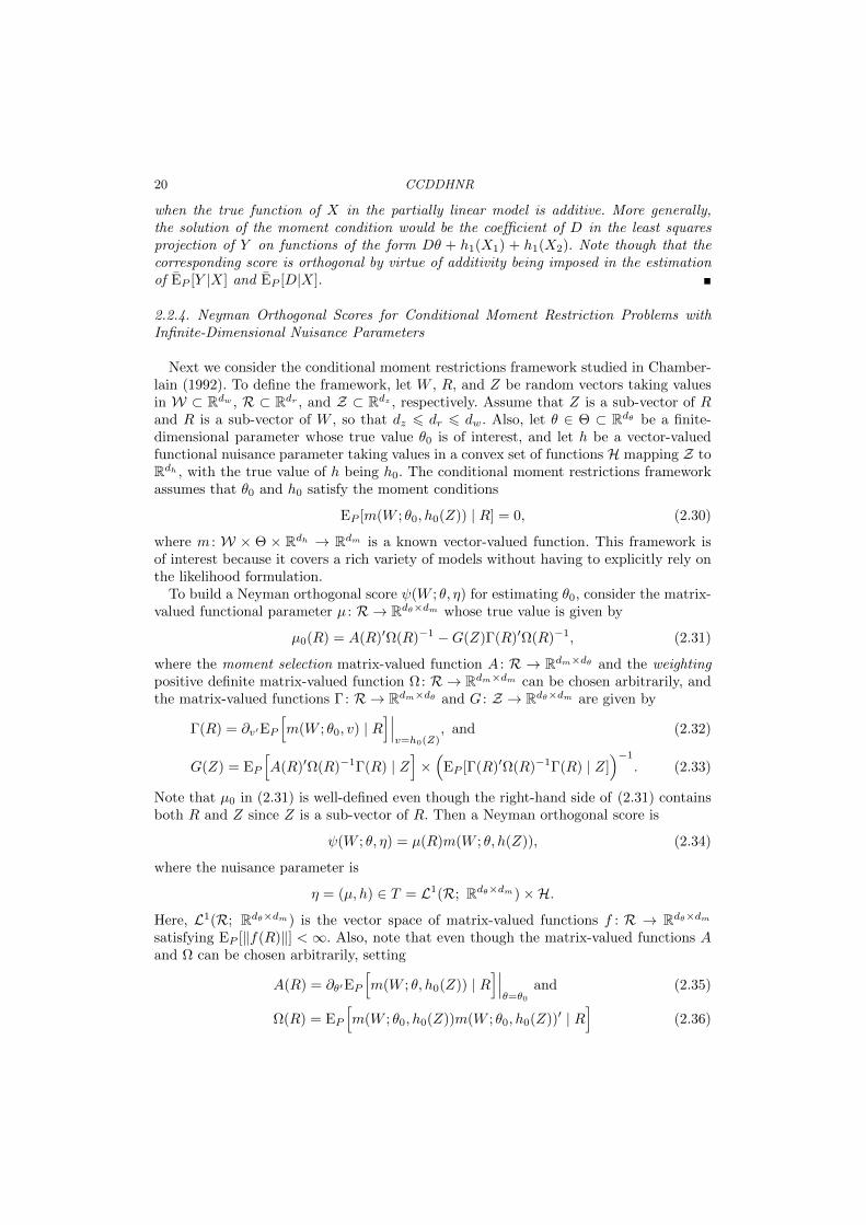
2.2.4. Neyman Orthogonal Scores for Conditional Moment Restriction Problems withInfinite-Dimensional Nuisance Parameters

Next we consider the conditional moment restrictions framework studied in Chamber-lain (1992). To define the framework, let W , R, and Z be random vectors taking valuesin W ⊂ Rdw , R ⊂ Rdr , and Z ⊂ Rdz , respectively. Assume that Z is a sub-vector of Rand R is a sub-vector of W , so that dz 6 dr 6 dw. Also, let θ ∈ Θ ⊂ Rdθ be a finite-dimensional parameter whose true value θ0 is of interest, and let h be a vector-valuedfunctional nuisance parameter taking values in a convex set of functions H mapping Z toRdh , with the true value of h being h0. The conditional moment restrictions frameworkassumes that θ0 and h0 satisfy the moment conditions

EP [m(W ; θ0, h0(Z)) | R] = 0, (2.30)

where m : W × Θ × Rdh → Rdm is a known vector-valued function. This framework isof interest because it covers a rich variety of models without having to explicitly rely onthe likelihood formulation.

To build a Neyman orthogonal score ψ(W ; θ, η) for estimating θ0, consider the matrix-valued functional parameter µ : R → Rdθ×dm whose true value is given by

µ0(R) = A(R)′Ω(R)−1 −G(Z)Γ(R)′Ω(R)−1, (2.31)

where the moment selection matrix-valued function A : R → Rdm×dθ and the weightingpositive definite matrix-valued function Ω: R → Rdm×dm can be chosen arbitrarily, andthe matrix-valued functions Γ: R → Rdm×dθ and G : Z → Rdθ×dm are given by

Γ(R) = ∂v′EP

[m(W ; θ0, v) | R

]∣∣∣v=h0(Z)

, and (2.32)

G(Z) = EP

[A(R)′Ω(R)−1Γ(R) | Z

]×(

EP [Γ(R)′Ω(R)−1Γ(R) | Z])−1

. (2.33)

Note that µ0 in (2.31) is well-defined even though the right-hand side of (2.31) containsboth R and Z since Z is a sub-vector of R. Then a Neyman orthogonal score is

ψ(W ; θ, η) = µ(R)m(W ; θ, h(Z)), (2.34)

where the nuisance parameter is

η = (µ, h) ∈ T = L1(R; Rdθ×dm)×H.

Here, L1(R; Rdθ×dm) is the vector space of matrix-valued functions f : R → Rdθ×dmsatisfying EP [‖f(R)‖] < ∞. Also, note that even though the matrix-valued functions Aand Ω can be chosen arbitrarily, setting

A(R) = ∂θ′EP

[m(W ; θ, h0(Z)) | R

]∣∣∣θ=θ0

and (2.35)

Ω(R) = EP

[m(W ; θ0, h0(Z))m(W ; θ0, h0(Z))′ | R

](2.36)

DML 21

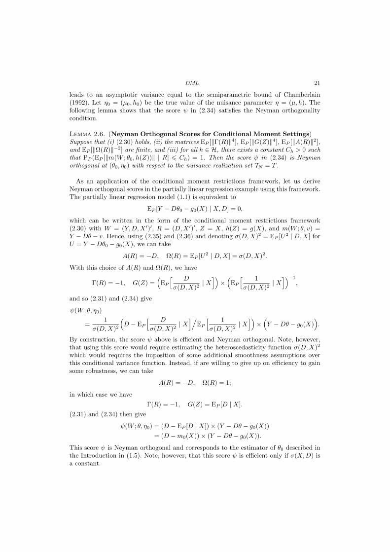
leads to an asymptotic variance equal to the semiparametric bound of Chamberlain(1992). Let η0 = (µ0, h0) be the true value of the nuisance parameter η = (µ, h). Thefollowing lemma shows that the score ψ in (2.34) satisfies the Neyman orthogonalitycondition.

Lemma 2.6. (Neyman Orthogonal Scores for Conditional Moment Settings)Suppose that (i) (2.30) holds, (ii) the matrices EP [‖Γ(R)‖4], EP [‖G(Z)‖4], EP [‖A(R)‖2],and EP [‖Ω(R)‖−2] are finite, and (iii) for all h ∈ H, there exists a constant Ch > 0 suchthat PP (EP [‖m(W ; θ0, h(Z))‖ | R] 6 Ch) = 1. Then the score ψ in (2.34) is Neymanorthogonal at (θ0, η0) with respect to the nuisance realization set TN = T .

As an application of the conditional moment restrictions framework, let us deriveNeyman orthogonal scores in the partially linear regression example using this framework.The partially linear regression model (1.1) is equivalent to

EP [Y −Dθ0 − g0(X) | X,D] = 0,

which can be written in the form of the conditional moment restrictions framework(2.30) with W = (Y,D,X ′)′, R = (D,X ′)′, Z = X, h(Z) = g(X), and m(W ; θ, v) =Y −Dθ − v. Hence, using (2.35) and (2.36) and denoting σ(D,X)2 = EP [U2 | D,X] forU = Y −Dθ0 − g0(X), we can take

A(R) = −D, Ω(R) = EP [U2 | D,X] = σ(D,X)2.

With this choice of A(R) and Ω(R), we have

Γ(R) = −1, G(Z) =(

EP

[ D

σ(D,X)2| X])×(

EP

[ 1

σ(D,X)2| X])−1

,

and so (2.31) and (2.34) give

ψ(W ; θ, η0)

=1

σ(D,X)2

(D − EP

[ D

σ(D,X)2| X]/

EP

[ 1

σ(D,X)2| X])×(Y −Dθ − g0(X)

).

By construction, the score ψ above is efficient and Neyman orthogonal. Note, however,that using this score would require estimating the heteroscedasticity function σ(D,X)2

which would requires the imposition of some additional smoothness assumptions overthis conditional variance function. Instead, if are willing to give up on efficiency to gainsome robustness, we can take

A(R) = −D, Ω(R) = 1;

in which case we have

Γ(R) = −1, G(Z) = EP [D | X].

(2.31) and (2.34) then give

ψ(W ; θ, η0) = (D − EP [D | X])× (Y −Dθ − g0(X))

= (D −m0(X))× (Y −Dθ − g0(X)).

This score ψ is Neyman orthogonal and corresponds to the estimator of θ0 described inthe Introduction in (1.5). Note, however, that this score ψ is efficient only if σ(X,D) isa constant.

22 CCDDHNR

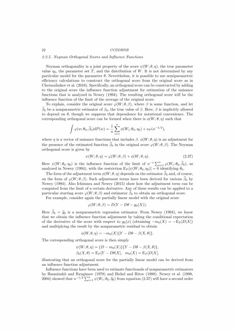
2.2.5. Neyman Orthogonal Scores and Influence Functions

Neyman orthogonality is a joint property of the score ψ(W ; θ, η), the true parametervalue η0, the parameter set T , and the distribution of W . It is not determined by anyparticular model for the parameter θ. Nevertheless, it is possible to use semiparametricefficiency calculations to construct the orthogonal score from the original score as inChernozhukov et al. (2016). Specifically, an orthogonal score can be constructed by addingto the original score the influence function adjustment for estimation of the nuisancefunctions that is analyzed in Newey (1994). The resulting orthogonal score will be theinfluence function of the limit of the average of the original score.

To explain, consider the original score ϕ(W ; θ, β), where β is some function, and let

β0 be a nonparametric estimator of β0, the true value of β. Here, β is implicitly allowedto depend on θ, though we suppress that dependence for notational convenience. Thecorresponding orthogonal score can be formed when there is φ(W ; θ, η) such that∫

ϕ(w; θ0, β0)dP (w) =1

n

n∑i=1

φ(Wi; θ0, η0) + oP (n−1/2),

where η is a vector of nuisance functions that includes β. φ(W ; θ, η) is an adjustment for

the presence of the estimated function β0 in the original score ϕ(W ; θ, β). The Neymanorthogonal score is given by

ψ(W ; θ, η) = ϕ(W ; θ, β) + φ(W ; θ, η). (2.37)

Here ψ(W ; θ0, η0) is the influence function of the limit of n−1∑ni=1 ϕ(Wi; θ0, β0), as

analyzed in Newey (1994), with the restriction EP [ψ(W ; θ0, η0)] = 0 identifying θ0.

The form of the adjustment term φ(W ; θ, η) depends on the estimator β0 and, of course,

on the form of ϕ(W ; θ, β). Such adjustment terms have been derived for various β0 byNewey (1994). Also Ichimura and Newey (2015) show how the adjustment term can becomputed from the limit of a certain derivative. Any of these results can be applied to aparticular starting score ϕ(W ; θ, β) and estimator β0 to obtain an orthogonal score.

For example, consider again the partially linear model with the original score

ϕ(W ; θ, β) = D(Y −Dθ − g0(X)).

Here β0 = g0 is a nonparametric regression estimator. From Newey (1994), we knowthat we obtain the influence function adjustment by taking the conditional expectationof the derivative of the score with respect to g0(x) (obtaining −m0(X) = −EP [D|X])and multiplying the result by the nonparametric residual to obtain

φ(W, θ, η) = −m0(X)Y −Dθ − β(X, θ).

The corresponding orthogonal score is then simply

ψ(W ; θ, η) = D −m0(X)Y −Dθ − β(X, θ),β0(X, θ) = EP [Y −Dθ|X], m0(X) = EP [D|X],

illustrating that an orthogonal score for the partially linear model can be derived froman influence function adjustment.

Influence functions have been used to estimate functionals of nonparametric estimatorsby Hasminskii and Ibragimov (1978) and Bickel and Ritov (1988). Newey et al. (1998,2004) showed that n−1/2

∑ni=1 ψ(Wi; θ0, η0) from equation (2.37) will have a second order

DML 23

remainder in η0, which is the key asymptotic property of orthogonal scores. Orthogonalityof influence functions in semiparametric models follows from van der Vaart (1991), asshown for higher order counterparts in Robins et al. (2008, 2017). Chernozhukov et al.(2016) point out that in general an orthogonal score can be constructed from an original

score and nonparametric estimator β0 by adding to the original score the adjustment termfor estimation of β0 as described above. This construction provides a way of obtainingan orthogonal score from any initial score ϕ(W ; θ, β) and nonparametric estimator β0.

3. DML: POST-REGULARIZED INFERENCE BASED ONNEYMAN-ORTHOGONAL ESTIMATING EQUATIONS

3.1. Definition of DML and Its Basic Properties

We assume that we have a sample (Wi)Ni=1, modeled as i.i.d. copies of W , whose law is

determined by the probability measure P onW. Estimation will be carried out using thefinite-sample analog of the estimating equations (2.9).

We assume that the true value η0 of the nuisance parameter η can be estimated by η0

using a part of the data (Wi)Ni=1. Different structured assumptions on η0 allow us to use

different machine-learning tools for estimating η0. For instance,

1) approximate sparsity for η0 with respect to some dictionary calls for the use offorward selection, lasso, post-lasso, `2-boosting, or some other sparsity-based tech-nique;

2) well-approximability of η0 by trees calls for the use of regression trees and randomforests;

3) well-approximability of η0 by sparse neural and deep neural nets calls for the useof `1-penalized neural and deep neural networks;

4) well-approximability of η0 by at least one model mentioned in 1)-3) above calls forthe use of an ensemble/aggregated method over the estimation methods mentionedin 1)-3).

There are performance guarantees for most of these ML methods that make it possibleto satisfy the conditions stated below. Ensemble and aggregation methods ensure thatthe performance guarantee is approximately no worse than the performance of the bestmethod.

We assume that N is divisible by K in order to simplify the notation. The followingalgorithm defines the simple cross-fitted DML as outlined in the Introduction.

Definition 3.1. (DML1) 1) Take a K-fold random partition (Ik)Kk=1 of observationindices [N ] = 1, ..., N such that the size of each fold Ik is n = N/K. Also, for eachk ∈ [K] = 1, . . . ,K, define Ick := 1, ..., N \ Ik. 2) For each k ∈ [K], construct a MLestimator

η0,k = η0((Wi)i∈Ick)

of η0, where η0,k is a random element in T , and where randomness depends only on thesubset of data indexed by Ick. 3) For each k ∈ [K], construct the estimator θ0,k as thesolution of the following equation:

En,k[ψ(W ; θ0,k, η0,k] = 0, (3.38)

24 CCDDHNR

where ψ is the Neyman orthogonal score, and En,k is the empirical expectation over thek-th fold of the data; that is, En,k[ψ(W )] = n−1

∑i∈Ik ψ(Wi). If achievement of exact 0

is not possible, define the estimator θ0,k of θ0 as an approximate εN -solution:∥∥∥En,k[ψ(W ; θ0,k, η0,k)]∥∥∥ 6 inf

θ∈Θ

∥∥∥En,k[ψ(W ; θ, η0,k)]∥∥∥+ εN , εN = o(δNN

−1/2), (3.39)

where (δN )N>1 is some sequence of positive constants converging to zero. 4) Aggregatethe estimators:

θ0 =1

K

K∑k=1

θ0,k. (3.40)

This approach generalizes the 50-50 cross-fitting method mentioned in the Introduc-tion. We now define a variation of this basic cross-fitting approach that may behavebetter in small samples.

Definition 3.2. (DML2) 1) Take a K-fold random partition (Ik)Kk=1 of observationindices [N ] = 1, ..., N such that the size of each fold Ik is n = N/K. Also, for eachk ∈ [K] = 1, . . . ,K, define Ick := 1, ..., N \ Ik. 2) For each k ∈ [K], construct a MLestimator

η0,k = η0((Wi)i∈Ick)

of η0, where η0,k is a random element in T , and where randomness depends only on the

subset of data indexed by Ick. 3) Construct the estimator θ0 as the solution to the followingequation:

1

K

K∑k=1

En,k[ψ(W ; θ0, η0,k)] = 0, (3.41)

where ψ is the Neyman orthogonal score, and En,k is the empirical expectation over thek-th fold of the data; that is, En,k[ψ(W )] = n−1

∑i∈Ik ψ(Wi). If achievement of exact 0

is not possible define the estimator θ0 of θ0 as an approximate εN -solution:∥∥∥ 1

K

K∑k=1

En,k[ψ(W ; θ0, η0,k)]]∥∥∥ 6 inf

θ∈Θ

∥∥∥ 1

K

K∑k=1

En,k[ψ(W ; θ0, η0,k)]]∥∥∥+ εN , (3.42)

for εN = o(δNN−1/2), where (δN )N>1 is some sequence of positive constants converging

to zero.

Remark 3.1. (Recommendations) The choice of K has no asymptotic impact under ourconditions but, of course, the choice of K may matter in small samples. Intuitively, largervalues of K provide more observations in Ick from which to estimate the high-dimensionalnuisance functions, which seems to be the more difficult part of the problem. We havefound moderate values of K, such as 4 or 5, to work better than K = 2 in a variety ofempirical examples and in simulations. Moreover, we generally recommend DML2 overDML1 though in some problems like estimation of ATE in the interactive model, which wediscuss later, there is no difference between the two approaches. In most other problems,DML2 is better behaved since the pooled empirical Jacobian for the equation in (3.41)exhibits more stable behavior than the separate empirical Jacobians for the equation in(3.38).

DML 25

3.2. Moment Condition Models with Linear Scores

We first consider the case of linear scores, where

ψ(w; θ, η) = ψa(w; η)θ + ψb(w; η), for all w ∈ W, θ ∈ Θ, η ∈ T. (3.43)

Let c0 > 0, c1 > 0, s > 0, q > 2 be some finite constants such that c0 6 c1; and letδNN>1 and ∆NN>1 be some sequences of positive constants converging to zero suchthat δN > N−1/2. Also, let K > 2 be some fixed integer, and let PNN>1 be somesequence of sets of probability distributions P of W on W.

Assumption 3.1. (Linear Scores with Approximate Neyman Orthogonality) For all N >3 and P ∈ PN , the following conditions hold. (i) The true parameter value θ0 obeys(2.9). (ii) The score ψ is linear in the sense of (3.43). (iii) The map η 7→ EP [ψ(W ; θ, η)]is twice continuously Gateaux-differentiable on T . (iv) The score ψ obeys the Neymanorthogonality or, more generally, the Neyman λN near-orthogonality condition at (θ0, η0)with respect to the nuisance realization set TN ⊂ T for

λN := supη∈TN

∥∥∥∂ηEPψ(W ; θ0, η0)[η − η0]∥∥∥ 6 δNN−1/2.

(v) The identification condition holds; namely, the singular values of the matrix

J0 := EP [ψa(W ; η0)]

are between c0 and c1.

Assumption 3.1 requires scores to be Neyman orthogonal or near-orthogonal and im-poses mild smoothness requirements as well as the canonical identification condition.

Assumption 3.2. (Score Regularity and Quality of Nuisance Parameter Estimators) Forall N > 3 and P ∈ PN , the following conditions hold. (i) Given a random subset I of[N ] of size n = N/K, the nuisance parameter estimator η0 = η0((Wi)i∈Ic) belongs tothe realization set TN with probability at least 1 − ∆N , where TN contains η0 and isconstrained by the next conditions. (ii) The moment conditions hold:

mN := supη∈TN

(EP [‖ψ(W ; θ0, η)‖q])1/q 6 c1,

m′N := supη∈TN

(EP [‖ψa(W ; η)‖q])1/q 6 c1.

(iii) The following conditions on the statistical rates rN , r′N , and λ′N hold:

rN := supη∈TN

‖EP [ψa(W ; η)]− EP [ψa(W ; η0)]‖ 6 δN ,

r′N := supη∈TN

(EP [‖ψ(W ; θ0, η)− ψ(W ; θ0, η0)‖2])1/2 6 δN ,

λ′N := supr∈(0,1),η∈TN

‖∂2rEP [ψ(W ; θ0, η0 + r(η − η0))]‖ 6 δN/

√N.

(iv) The variance of the score ψ is non-degenerate: All eigenvalues of the matrix

EP [ψ(W ; θ0, η0)ψ(W ; θ0, η0)′]

are bounded from below by c0.

26 CCDDHNR

Assumptions 3.2(i)-(iii) state that the estimator of the nuisance parameter belongsto the realization set TN ⊂ T , which is a shrinking neighborhood of η0, which contractsaround η0 with the rate determined by the “statistical” rates rN , r′N , and λ′N . These ratesare not given in terms of the norm ‖ · ‖T on T , but rather are the intrinsic rates thatare most connected to the statistical problem at hand. However, in smooth problems,as discussed below this translates, in the worst cases, to the crude requirement that thenuisance parameters are estimated at the rate o(N−1/4).

The conditions in Assumption 3.2 embody refined requirements on the quality of nui-sance parameter estimators. In many applications, where (θ, η) 7→ ψ(W ; θ, η) is smooth,we can bound

rN . εN , r′N . εN , λ′N . ε2N , (3.44)

where εN is the upper bound on the rate of convergence of η0 to η0 with respect to thenorm ‖ · ‖T = ‖ · ‖P,2:

‖η0 − η‖T . εN .Note that TN can be chosen as the set of η that is within a neighborhood of size εN ofη0, possibly with other restrictions, in this case. If only (3.44) holds, Assumption 3.2,particularly λ′N = o(N−1/2), imposes the (crude) rate requirement

εN = o(N−1/4). (3.45)

This rate is achievable for many ML methods under structured assumptions on the nui-sance parameters. See, among many others, Bickel et al. (2009), Buhlmann and van deGeer (2011), Belloni et al. (2011), Belloni and Chernozhukov (2011), Belloni et al. (2012),and Belloni and Chernozhukov (2013) for `1-penalized and related methods in a varietyof sparse models; Kozbur (2016) for forward selection in sparse models; Luo and Spindler(2016) for L2-boosting in sparse linear models; Wager and Walther (2016) for concen-tration results for a class of regression trees and random forests; and Chen and White(1999) for a class of neural nets.

However, the presented conditions allow for more refined statements than (3.45). Wenote that many important structured problems – such as estimation of parameters inpartially linear regression models, estimation of parameters in partially linear structuralequation models, and estimation of average treatment effects under unconfoundedness– are such that some cross-derivatives vanish, allowing more refined requirements than(3.45). This feature allows us to require much finer conditions on the quality of the nui-sance parameter estimators than the crude bound (3.45). For example, in many problems

λ′N = 0, (3.46)

because the second derivatives vanish,

∂2rEP [ψ(W ; θ0, η0 + r(η − η0))] = 0.

This occurs in the following important examples:

• the optimal instrument problem; see Belloni et al. (2012).

• the partially linear regression model when m0(X) = 0 or is otherwise known; seeSection 4.

• the treatment effect examples when the propensity score is known, which includesrandomized control trials as an important special case; see Section 5.

DML 27

If both (3.44) and (3.46) hold, Assumption 3.2, particularly rN = o(1) and r′N = o(1),imposes the weakest possible rate requirement:

εN = o(1).

We note that similar refined rates have appeared in the context of estimation of treatmenteffects in high-dimensional settings under sparsity; see Farrell (2015) and Athey et al.(2016) and related discussion in Remark 5.2. Our refined rate results complement thiswork by applying to a broad class of estimation contexts, including estimation of averagetreatment effects, and to a broad set of ML estimators.

Theorem 3.1. (Properties of the DML) Suppose that Assumptions 3.1 and 3.2 hold.In addition, suppose that δN > N−1/2 for all N > 1. Then the DML1 and DML2estimators θ0 concentrate in a 1/

√N neighborhood of θ0 and are approximately linear

and centered Gaussian:

√Nσ−1(θ0 − θ0) =

1√N

N∑i=1

ψ(Wi) +OP (ρN ) ; N(0, Id), (3.47)

uniformly over P ∈ PN , where the size of the remainder term obeys

ρN := N−1/2 + rN + r′N +N1/2λN +N1/2λ′N . δN , (3.48)

ψ(·) := −σ−1J−10 ψ(·, θ0, η0) is the influence function, and the approximate variance is

σ2 := J−10 EP [ψ(W ; θ0, η0)ψ(W ; θ0, η0)′](J−1

0 )′.

The result establishes that the estimator based on the orthogonal scores achieves theroot-N rate of convergence and is approximately normally distributed. It is notewor-thy that this convergence result, both the rate of concentration and the distributionalapproximation, holds uniformly with respect to P varying over an expanding class ofprobability measures PN . This means that the convergence holds under any sequence ofprobability distributions (PN )N>1 with PN ∈ PN for each N , which in turn implies thatthe results are robust with respect to perturbations of a given P along such sequences.The same property can be shown to fail for methods not based on orthogonal scores.

Theorem 3.2. (Variance Estimator for DML) Suppose that Assumptions 3.1 and3.2 hold. In addition, suppose that δN > N−[(1−2/q)∧1/2] for all N > 1. Consider thefollowing estimator of the asymptotic variance matrix of

√N(θ0 − θ0):

σ2 = J−10

1

K

K∑k=1

En,k[ψ(W ; θ0, η0,k)ψ(W ; θ0, η0,k)′](J−10 )′,

where

J0 =1

K

K∑k=1

En,k[ψa(W ; η0,k)],

and θ0 is either the DML1 or the DML2 estimator. This estimator concentrates aroundthe true variance matrix σ2,

σ2 = σ2 +OP (%N ), %N := N−[(1−2/q)∧1/2] + rN + r′N . δN .

28 CCDDHNR

Moreover, σ2 can replace σ2 in the statement of Theorem 3.1 with the size of the remain-der term updated as ρN = N−[(1−2/q)∧1/2] + rN + r′N +N1/2λN +N1/2λ′N .

Theorems 3.1 and 3.2 can be used for standard construction of confidence regions whichare uniformly valid over a large, interesting class of models:

Corollary 3.1. (Uniformly Valid Confidence Bands) Under the conditions ofTheorem 3.2, suppose we are interested in the scalar parameter `′θ0 for some dθ × 1vector `. Then the confidence interval

CI :=[`′θ0 ± Φ−1(1− α/2)

√`′σ2`/N

]obeys

supP∈PN

∣∣∣PP (θ0 ∈ CI)− (1− α)∣∣∣→ 0.

Indeed, the above theorem implies that CI obeys PPN (θ0 ∈ CI) → (1 − α) under anysequence PN ∈ PN , which implies that these claims hold uniformly in P ∈ PN . Forexample, one may choose PN such that, for some εN → 0

supP∈PN

|PP (θ0 ∈ CI)− (1− α)| 6 |PPN (θ0 ∈ CI)− (1− α)|+ εN → 0.

Next we note that the estimators need not be semi-parametrically efficient, but undersome conditions they can be.

Corollary 3.2. (Cases with Semi-parametric Efficiency) Under the conditions ofTheorem 3.1, if the score ψ is efficient for estimating θ0 at a given P ∈ P ⊂ PN , in thesemi-parametric sense as defined in van der Vaart (1998), then the large sample varianceσ2

0 of θ0 reaches the semi-parametric efficiency bound at this P relative to the model P.

3.3. Models with Nonlinear Scores

Let c0 > 0, c1 > 0, a > 1, v > 0, s > 0, and q > 2 be some finite constants, andlet δNN>1, ∆NN>1, and τNN>1 be some sequences of positive constants converg-ing to zero. To derive the properties of the DML estimator, we will use the followingassumptions.

Assumption 3.3. (Nonlinear Moment Condition Problem with Approximate NeymanOrthogonality) For all N > 3 and P ∈ PN , the following conditions hold. (i) The trueparameter value θ0 obeys (2.9), and Θ contains a ball of radius c1N

−1/2 logN centeredat θ0. (ii) The map (θ, η) 7→ EP [ψ(W ; θ, η)] is twice continuously Gateaux-differentiableon Θ× T . (iii) For all θ ∈ Θ, the identification relation

2‖EP [ψ(W ; θ, η0)]‖ > ‖J0(θ − θ0)‖ ∧ c0is satisfied, for the Jacobian matrix

J0 := ∂θ′

EP [ψ(W ; θ, η0)]∣∣∣θ=θ0

having singular values between c0 and c1. (iv) The score ψ obeys the Neyman orthogonality

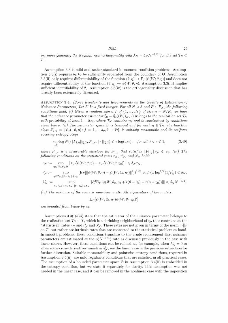
DML 29

or, more generally the Neyman near-orthogonality with λN = δNN−1/2 for the set TN ⊂

T .

Assumption 3.3 is mild and rather standard in moment condition problems. Assump-tion 3.3(i) requires θ0 to be sufficiently separated from the boundary of Θ. Assumption3.3(ii) only requires differentiability of the function (θ, η) 7→ EP [ψ(W ; θ, η)] and does notrequire differentiability of the function (θ, η) 7→ ψ(W ; θ, η). Assumption 3.3(iii) impliessufficient identifiability of θ0. Assumption 3.3(iv) is the orthogonality discussion that hasalready been extensively discussed.

Assumption 3.4. (Score Regularity and Requirements on the Quality of Estimation ofNuisance Parameters) Let K be a fixed integer. For all N > 3 and P ∈ PN , the followingconditions hold. (i) Given a random subset I of 1, . . . , N of size n = N/K, we havethat the nuisance parameter estimator η0 = η0((Wi)i∈Ic) belongs to the realization set TNwith probability at least 1−∆N , where TN contains η0 and is constrained by conditionsgiven below. (ii) The parameter space Θ is bounded and for each η ∈ TN , the functionclass F1,η = ψj(·, θ, η) : j = 1, ..., dθ, θ ∈ Θ is suitably measurable and its uniformcovering entropy obeys

supQ

logN(ε‖F1,η‖Q,2,F1,η, ‖ · ‖Q,2) 6 v log(a/ε), for all 0 < ε 6 1, (3.49)

where F1,η is a measurable envelope for F1,η that satisfies ‖F1,η‖P,q 6 c1. (iii) Thefollowing conditions on the statistical rates rN , r′N , and λ′N hold:

rN := supη∈TN ,θ∈Θ

‖EP [ψ(W ; θ, η)− EP [ψ(W ; θ, η0)]‖ 6 δNτN ,

r′N := supη∈TN ,‖θ−θ0‖6τN

(EP [‖ψ(W ; θ, η)− ψ(W ; θ0, η0)‖2])1/2 and r′N log1/2(1/r′N ) 6 δN ,

λ′N := supr∈(0,1),η∈TN ,‖θ−θ0‖6τN

‖∂2rEP [ψ(W ; θ0, η0 + r(θ − θ0) + r(η − η0))]‖ 6 δNN−1/2.

(iv) The variance of the score is non-degenerate: All eigenvalues of the matrix

EP [ψ(W ; θ0, η0)ψ(W ; θ0, η0)′]

are bounded from below by c0.

Assumptions 3.3(i)-(iii) state that the estimator of the nuisance parameter belongs tothe realization set TN ⊂ T , which is a shrinking neighborhood of η0 that contracts at the“statistical” rates rN and r′N and λ′N . These rates are not given in terms of the norm ‖·‖Ton T , but rather are intrinsic rates that are connected to the statistical problem at hand.In smooth problems, these conditions translate to the crude requirement that nuisanceparameters are estimated at the o(N−1/4) rate as discussed previously in the case withlinear scores. However, these conditions can be refined as, for example, when λ′N = 0 orwhen some cross-derivatives vanish in λ′N ; see the linear case in the previous subsection forfurther discussion. Suitable measurability and pointwise entropy conditions, required inAssumption 3.4(ii), are mild regularity conditions that are satisfied in all practical cases.The assumption of a bounded parameter space Θ in Assumption 3.4(ii) is embedded inthe entropy condition, but we state it separately for clarity. This assumption was notneeded in the linear case, and it can be removed in the nonlinear case with the imposition

30 CCDDHNR

of more complicated Huber-like regularity conditions. Assumption 3.4(iii) is a set of mildgrowth conditions.

Remark 3.2. (Rate Requirements on Nuisance Parameter Estimators) Similar to thediscussion in the linear case, the conditions in Assumption 3.4 are very flexible andembody refined requirements on the quality of the nuisance parameter estimators. Theconditions essentially reduce to the previous conditions in the linear case, with the excep-tion of compactness, which is imposed to make the conditions easy to verify in non-linearcases.

Theorem 3.3. (Properties of the DML for Nonlinear Scores) Suppose that As-sumptions 3.3 and 3.4 hold. In addition, suppose that δN > N−1/2+1/q logN and thatN−1/2 logN 6 τN 6 δN for all N > 1. Then the DML1 and DML2 estimators θ0

concentrate in a 1/√N neighborhood of θ0, and are approximately linear and centered

Gaussian:

√Nσ−1(θ0 − θ0) =

1√N

N∑i=1

ψ(Wi) +OP (ρN ) ; N(0, I),

uniformly over P ∈ PN , where the size of the remainder term obeys

ρN := N−1/2+1/q logN + r′N log1/2(1/r′N ) +N1/2λN +N1/2λ′N . δN ,

ψ(·) := −σ−10 J−1

0 ψ(·, θ0, η0) is the influence function, and the approximate variance is

σ2 := J−10 EP [ψ(W ; θ0, η0)ψ(W ; θ0, η0)′](J−1

0 )′.

Moreover, in the statement above σ2 can be replaced by a consistent estimator σ2, obeyingσ2 = σ2 + oP (%N ) uniformly in P ∈ PN , with the size of the remainder term updatedas ρN = ρN + %N . Furthermore, Corollaries 3.1 and 3.2 continue to hold under theconditions of this theorem.

3.4. Finite-Sample Adjustments to Incorporate Uncertainty Induced by Sample Splitting

The estimation technique developed in this paper relies on subsamples obtained by ran-domly partitioning the sample: an auxiliary sample for estimating the nuisance functionsand a main sample for estimating the parameter of interest. Although the specific samplepartition has no impact on estimation results asymptotically, the effect of the particularrandom split on the estimate can be important in finite samples. To make the resultsmore robust with respect to the partitioning, we propose to repeat the DML estimatorS times, obtaining the estimates

θs0, s = 1, . . . , S.

Features of these estimates may then provide insight into the sensitivity of results tothe sample splitting, and we can report results that incorporate features of this set ofestimates that should be less driven by any particular sample-splitting realization.

Definition 3.3. (Incorporating the Impact of Sample Splitting using Meanand Median Methods) For point estimation, we suggest reporting either

θmean0 =

1

S

S∑s=1

θs0 or θmedian0 = medianθs0Ss=1,

DML 31

where the median operation is applied coordinatewise. To quantify and incorporate thevariation introduced by sample splitting, we consider variance estimators:

σ2,mean =1

S

S∑s=1

(σ2s + (θs − θmean)(θs − θmean)′

), (3.50)

and a more robust version,

σ2,median = medianσ2s + ((θs − θmedian)(θs − θmedian)′Ss=1, (3.51)

where the median picks out the matrix with median operator norm, which preserve non-negative definiteness.

We recommend using medians, reporting θmedian0 and σ2Median, as these quantities are

more robust to outliers.

Corollary 3.3. If S is fixed, as N →∞ and maintaining either Assumptions 3.1 and3.2 or Assumptions 3.3 and 3.4 as appropriate, θmean

0 and θmedian0 are first-order equiva-

lent to θ0 and obey the conclusions of Theorems 3.1 and 3.2 or of Theorem 3.3. Moreover,σ2,median and σ2,mean can replace σ in the statement of the appropriate theorems.

It would be interesting to investigate the behavior under the regime where S →∞ asN →∞.

4. INFERENCE IN PARTIALLY LINEAR MODELS

4.1. Inference in Partially Linear Regression Models

Here we revisit the partially linear regression model

Y = Dθ0 + g0(X) + U, EP [U | X,D] = 0, (4.52)

D = m0(X) + V, EP [V | X] = 0. (4.53)

The parameter of interest is the regression coefficient θ0. If D is conditionally exogenous(as good as randomly assigned conditional on covariates), then θ0 measures the averagecausal/treatment effect of D on potential outcomes.

The first approach to inference on θ0, which we described in the Introduction, is toemploy the DML method using the score function

ψ(W ; θ, η) := Y −Dθ − g(X)(D −m(X)), η = (g,m), (4.54)

where W = (Y,D,X) and g and m are P -square-integrable functions mapping the sup-port ofX to R. It is easy to see that θ0 satisfies the moment condition EPψ(W ; θ0, η0) = 0,and also the orthogonality condition ∂ηEPψ(W ; θ0, η0)[η − η0] = 0 where η0 = (g0,m0).

A second approach employs the Robinson-style “partialling-out” score function

ψ(W ; θ, η) := Y − `(X)− θ(D −m(X))(D −m(X)), η = (`,m), (4.55)

where W = (Y,D,X) and ` and m are P -square-integrable functions mapping the sup-port of X to R. This gives an alternative parameterization of the score function above,and using this score is first-order equivalent to using the previous score. It is easy to seethat θ0 satisfies the moment condition EPψ(W ; θ0, η0) = 0, and also the orthogonalitycondition ∂ηEPψ(W ; θ0, η0)[η − η0] = 0, for η0 = (`0,m0), where `0(X) = EP [Y |Z].

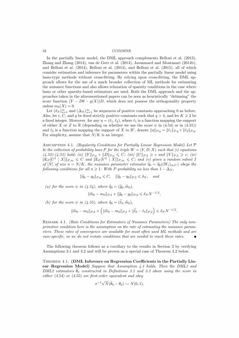
32 CCDDHNR

In the partially linear model, the DML approach complements Belloni et al. (2013),Zhang and Zhang (2014), van de Geer et al. (2014), Javanmard and Montanari (2014b),and Belloni et al. (2014), Belloni et al. (2014), and Belloni et al. (2015), all of whichconsider estimation and inference for parameters within the partially linear model usinglasso-type methods without cross-fitting. By relying upon cross-fitting, the DML ap-proach allows for the use of a much broader collection of ML methods for estimatingthe nuisance functions and also allows relaxation of sparsity conditions in the case wherelasso or other sparsity-based estimators are used. Both the DML approach and the ap-proaches taken in the aforementioned papers can be seen as heuristically “debiasing” thescore function (Y − Dθ − g(X))D, which does not possess the orthogonality propertyunless m0(X) = 0.

Let (δN )∞n=1 and (∆N )∞n=1 be sequences of positive constants approaching 0 as before.Also, let c, C, and q be fixed strictly positive constants such that q > 4, and let K > 2 bea fixed integer. Moreover, for any η = (`1, `2), where `1 is a function mapping the supportof either X or Z to R (depending on whether we use the score ψ in (4.54) or in (4.55))and `2 is a function mapping the support of X to Rl, denote ‖η‖P,q = ‖`1‖P,q ∨ ‖`2‖P,q.For simplicity, assume that N/K is an integer.

Assumption 4.1. (Regularity Conditions for Partially Linear Regression Model) Let Pbe the collection of probability laws P for the triple W = (Y,D,X) such that (i) equations(4.52)-(4.53) hold; (ii) ‖Y ‖P,q + ‖D‖P,q 6 C; (iii) ‖U‖P,2 > c and ‖V ‖P,2 > c; (iv)‖EP [U2 | X]‖P,∞ 6 C and ‖EP [V 2 | X]‖P,∞ 6 C; and (v) given a random subset Iof [N ] of size n = N/K, the nuisance parameter estimator η0 = η0((Wi)i∈Ic) obeys thefollowing conditions for all n > 1: With P -probability no less than 1−∆N ,

‖η0 − η0‖P,q 6 C, ‖η0 − η0‖P,2 6 δN , and

(a) for the score ψ in (4.54), where η0 = (g0, m0),

‖m0 −m0‖P,2 × ‖g0 − g0‖P,2 6 δNN−1/2,

(b) for the score ψ in (4.55), where η0 = (0, m0),

‖m0 −m0‖P,2 ×(‖m0 −m0‖P,2 + ‖0 − `0‖P,2) 6 δNN−1/2.

Remark 4.1. (Rate Conditions for Estimators of Nuisance Parameters) The only non-primitive condition here is the assumption on the rate of estimating the nuisance param-eters. These rates of convergence are available for most often used ML methods and arecase-specific, so we do not restate conditions that are needed to reach these rates.

The following theorem follows as a corollary to the results in Section 3 by verifyingAssumptions 3.1 and 3.2 and will be proven as a special case of Theorem 4.2 below.

Theorem 4.1. (DML Inference on Regression Coefficients in the Partially Lin-ear Regression Model) Suppose that Assumption 4.1 holds. Then the DML1 andDML2 estimators θ0 constructed in Definitions 3.1 and 3.2 above using the score ineither (4.54) or (4.55) are first-order equivalent and obey

σ−1√N(θ0 − θ0) ; N(0, 1),

DML 33

uniformly over P ∈ P, where σ2 = [EPV2]−1EP [V 2U2][EPV

2]−1. Moreover, the resultcontinues to hold if σ2 is replaced by σ2 defined in Theorem 3.2. Consequently, confidenceregions based upon the DML estimators θ0 have uniform asymptotic validity:

limN→∞

supP∈P

∣∣∣PP (θ0 ∈ [θ0 ± Φ−1(1− α/2)σ/√N ])− (1− α)

∣∣∣ = 0.

Remark 4.2. (Asymptotic Efficiency under Homoscedasticity) Under conditional ho-moscedasticity, i.e. E[U2|Z] = E[U2], the asymptotic variance σ2 reduces to E[V 2]−1E[U2],which is the semi-parametric efficiency bound for θ.

Remark 4.3. (Tightness of Conditions under Cross-Fitting) The conditions in Theorem4.1 are fairly sharp, though they are somewhat simplified for ease of presentation. Thesharpness can be understood by examining the case where the regression function g0 andthe propensity function m0 are sparse with sparsity indices sg N and sm N andare estimated by `1-penalized estimators g0 and m0 that have sparsity indices of orderssg and sm and converge to g0 and m0 at the rates

√sg/N and

√sm/N (ignoring logs).

The rate conditions in Assumption 4.1 then require (ignoring logs) that√sg/N

√sm/N N−1/2 ⇔ sgsm N,

which is much weaker than the condition

(sg)2 + (sm)2 N

(ignoring logs) required without sample splitting. For example, if the propensity functionm0 is very sparse (low sm), then the regression function is allowed to be quite dense (highsg), and vice versa. If the propensity function is known (sm = 0) or can be estimated atthe N−1/2 rate, then only consistency for g0 is needed. Such comparisons also extend toapproximately sparse models.

4.2. Inference in Partially Linear IV Models

Here we extend the partially linear regression model studied in Section 4.1 to allow forinstrumental variable (IV) identification. Specifically, we consider the model

Y = Dθ0 + g0(X) + U, EP [U | X,Z] = 0, (4.56)

Z = m0(X) + V, EP [V | X] = 0, (4.57)

where Z is the instrumental variable. As before, the parameter of interest is θ and itstrue value is θ0. If Z = D, the model (4.56)-(4.57) coincides with (4.52)-(4.53) but isotherwise different.

To estimate θ0 and to perform inference on it, we will use the score

ψ(W ; θ, η) := (Y −Dθ − g(X))(Z −m(X)), η = (g,m), (4.58)

where W = (Y,D,X,Z) and g and m are P -square-integrable functions mapping thesupport of X to R. Alternatively, we can use the Robinson-style score

ψ(W ; θ, η) := (Y − `(X)− θ(D − r(X)))(Z −m(X)), η = (`,m, r), (4.59)

where W = (Y,D,X,Z) and `, m, and r are P -square-integrable functions mapping thesupport of X to R. It is straightforward to verify that both scores satisfy the moment

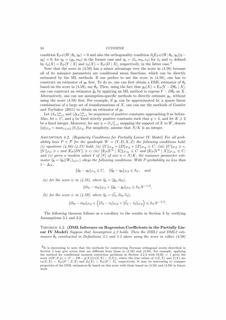
34 CCDDHNR

condition EPψ(W ; θ0, η0) = 0 and also the orthogonality condition ∂ηEPψ(W ; θ0, η0)[η−η0] = 0, for η0 = (g0,m0) in the former case and η0 = (`0,m0, r0) for `0 and r0 definedby `0(X) = EP [Y | X] and r0(X) = EP [D | X], respectively, in the latter case.8

Note that the score in (4.59) has a minor advantage over the score in (4.58) becauseall of its nuisance parameters are conditional mean functions, which can be directlyestimated by the ML methods. If one prefers to use the score in (4.58), one has toconstruct an estimator of g0 first. To do so, one can first obtain a DML estimator of θ0

based on the score in (4.59), say θ0. Then, using the fact that g0(X) = EP [Y −Dθ0 | X],one can construct an estimator g0 by applying an ML method to regress Y −Dθ0 on X.Alternatively, one can use assumption-specific methods to directly estimate g0, withoutusing the score (4.59) first. For example, if g0 can be approximated by a sparse linearcombination of a large set of transformations of X, one can use the methods of Gautierand Tsybakov (2011) to obtain an estimator of g0.

Let (δN )∞n=1 and (∆N )∞n=1 be sequences of positive constants approaching 0 as before.Also, let c, C, and q be fixed strictly positive constants such that q > 4, and let K > 2be a fixed integer. Moreover, for any η = (`j)

lj=1 mapping the support of X to Rl, denote

‖η‖P,q = max16j6l ‖`j‖P,q. For simplicity, assume that N/K is an integer.

Assumption 4.2. (Regularity Conditions for Partially Linear IV Model) For all prob-ability laws P ∈ P for the quadruple W = (Y,D,X,Z) the following conditions hold:(i) equations (4.56)-(4.57) hold; (ii) ‖Y ‖P,q + ‖D‖P,q + ‖Z‖P,q 6 C; (iii) ‖U‖P,2 > c,‖V ‖P,2 > c and |EP [DV ]| > c; (iv) ‖EP [U2 | X]‖P,∞ 6 C and ‖EP [V 2 | X]‖P,∞ 6 C;and (v) given a random subset I of [N ] of size n = N/K, the nuisance parameter esti-mator η0 = η0((Wi)i∈Ic) obeys the following conditions: With P -probability no less than1−∆N ,

‖η0 − η0‖P,q 6 C, ‖η0 − η0‖P,2 6 δN , and

(a) for the score ψ in (4.58), where η0 = (g0, m0),

‖m0 −m0‖P,2 × ‖g0 − g0‖P,2 6 δNN−1/2,

(b) for the score ψ in (4.59), where η0 = (0, m0, r0),

‖m0 −m0‖P,2 ×(‖r0 − r0‖P,2 + ‖0 − `0‖P,2) 6 δNN−1/2.

The following theorem follows as a corollary to the results in Section 3 by verifyingAssumptions 3.1 and 3.2.

Theorem 4.2. (DML Inference on Regression Coefficients in the Partially Lin-ear IV Model) Suppose that Assumption 4.2 holds. Then the DML1 and DML2 esti-mators θ0 constructed in Definitions 3.1 and 3.2 above using the score in either (4.58)

8It is interesting to note that the methods for constructing Neyman orthogonal scores described inSection 2 may give scores that are different from those in (4.58) and (4.59). For example, applyingthe method for conditional moment restriction problems in Section 2.2.4 with Ω(R) = 1 gives thescore ψ(W ; θ, η) = (Y − Dθ − g(X))(r(Z,X) − f(X)), where the true values of r(Z,X) and f(X) arer0(Z,X) = EP [D | Z,X] and f0(X) = EP [D | X], respectively. It may be interesting to compare

properties of the DML estimators θ0 based on this score with those based on (4.58) and (4.59) in futurework.

DML 35

or (4.59) are first-order equivalent and obey

σ−1√N(θ0 − θ0) ; N(0, 1),

uniformly over P ∈ P, where σ2 = [EPV2]−1EP [V 2U2][EPV

2]−1. Moreover, the resultcontinues to hold if σ2 is replaced by σ2 defined in Theorem 3.2. Consequently, confidenceregions based upon the DML estimators θ0 have uniform asymptotic validity:

limN→∞

supP∈P

∣∣∣PP (θ0 ∈ [θ0 ± Φ−1(1− α/2)σ/√N ])− (1− α)

∣∣∣ = 0.

5. INFERENCE ON TREATMENT EFFECTS IN THE INTERACTIVE MODEL

5.1. Inference on ATE and ATTE

In this section, we specialize the results of Section 3 to estimating treatment effects underthe unconfoundedness assumption of Rosenbaum and Rubin (1983). Within this setting,there is a large classical literature focused on low-dimensional settings that providesmethods for adjusting for confounding variables including regression methods, propen-sity score adjustment methods, matching methods, and “doubly-robust” combinationsof these methods; see, for example, Robins and Rotnitzky (1995), Hahn (1998), Hiranoet al. (2003), and Abadie and Imbens (2006) as well as the textbook overview providedin Imbens and Rubin (2015). In this section, we present results that complement this im-portant classic work as well as the rapidly expanding body of work on estimation underunconfoundedness using ML methods; see, among others, Athey et al. (2016), Belloniet al. (2013), Belloni et al. (2014), Farrell (2015), and Imai and Ratkovic (2013).

We specifically consider estimation of average treatment effects when treatment effectsare fully heterogeneous and the treatment variable is binary, D ∈ 0, 1. We considervectors (Y,D,X) such that

Y = g0(D,X) + U, EP [U | X,D] = 0, (5.60)

D = m0(X) + V, EP [V | X] = 0. (5.61)

Since D is not additively separable, this model is more general than the partially linearmodel for the case of binary D. A common target parameter of interest in this model isthe average treatment effect (ATE),9

θ0 = EP [g0(1, X)− g0(0, X)].

Another common target parameter is the average treatment effect for the treated (ATTE),

θ0 = EP [g0(1, X)− g0(0, X)|D = 1].

The confounding factors X affect the policy variable via the propensity score m0(X)and the outcome variable via the function g0(D,X). Both of these functions are unknownand potentially complicated, and we can employ ML methods to learn them.

We proceed to set up moment conditions with scores obeying orthogonality conditions.For estimation of the ATE, we employ

ψ(W ; θ, η) := (g(1, X)− g(0, X)) +D(Y − g(1, X))

m(X)− (1−D)(Y − g(0, X))

1−m(X)− θ, (5.62)

9Without unconfoundedness/conditional exogeneity, these quantities measure association, and couldbe referred to as average predictive effect (APE) and average predictive effect for the exposed (APEX).Inferential results for these objects would follow immediately from Theorem 5.1.

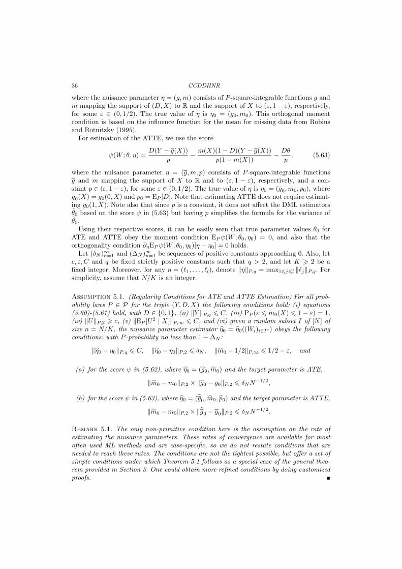
36 CCDDHNR

where the nuisance parameter η = (g,m) consists of P -square-integrable functions g andm mapping the support of (D,X) to R and the support of X to (ε, 1− ε), respectively,for some ε ∈ (0, 1/2). The true value of η is η0 = (g0,m0). This orthogonal momentcondition is based on the influence function for the mean for missing data from Robinsand Rotnitzky (1995).

For estimation of the ATTE, we use the score

ψ(W ; θ, η) =D(Y − g(X))

p− m(X)(1−D)(Y − g(X))

p(1−m(X))− Dθ

p, (5.63)

where the nuisance parameter η = (g,m, p) consists of P -square-integrable functionsg and m mapping the support of X to R and to (ε, 1 − ε), respectively, and a con-stant p ∈ (ε, 1− ε), for some ε ∈ (0, 1/2). The true value of η is η0 = (g0,m0, p0), whereg0(X) = g0(0, X) and p0 = EP [D]. Note that estimating ATTE does not require estimat-ing g0(1, X). Note also that since p is a constant, it does not affect the DML estimatorsθ0 based on the score ψ in (5.63) but having p simplifies the formula for the variance ofθ0.

Using their respective scores, it can be easily seen that true parameter values θ0 forATE and ATTE obey the moment condition EPψ(W ; θ0, η0) = 0, and also that theorthogonality condition ∂ηEPψ(W ; θ0, η0)[η − η0] = 0 holds.

Let (δN )∞n=1 and (∆N )∞n=1 be sequences of positive constants approaching 0. Also, letc, ε, C and q be fixed strictly positive constants such that q > 2, and let K > 2 be afixed integer. Moreover, for any η = (`1, . . . , `l), denote ‖η‖P,q = max16j6l ‖`j‖P,q. Forsimplicity, assume that N/K is an integer.

Assumption 5.1. (Regularity Conditions for ATE and ATTE Estimation) For all prob-ability laws P ∈ P for the triple (Y,D,X) the following conditions hold: (i) equations(5.60)-(5.61) hold, with D ∈ 0, 1, (ii) ‖Y ‖P,q 6 C, (iii) PP (ε 6 m0(X) 6 1− ε) = 1,(iv) ‖U‖P,2 > c, (v) ‖EP [U2 | X]‖P,∞ 6 C, and (vi) given a random subset I of [N ] ofsize n = N/K, the nuisance parameter estimator η0 = η0((Wi)i∈Ic) obeys the followingconditions: with P -probability no less than 1−∆N :

‖η0 − η0‖P,q 6 C, ‖η0 − η0‖P,2 6 δN , ‖m0 − 1/2‖P,∞ 6 1/2− ε, and

(a) for the score ψ in (5.62), where η0 = (g0, m0) and the target parameter is ATE,

‖m0 −m0‖P,2 × ‖g0 − g0‖P,2 6 δNN−1/2,

(b) for the score ψ in (5.63), where η0 = (g0, m0, p0) and the target parameter is ATTE,

‖m0 −m0‖P,2 × ‖g0 − g0‖P,2 6 δNN−1/2.

Remark 5.1. The only non-primitive condition here is the assumption on the rate ofestimating the nuisance parameters. These rates of convergence are available for mostoften used ML methods and are case-specific, so we do not restate conditions that areneeded to reach these rates. The conditions are not the tightest possible, but offer a set ofsimple conditions under which Theorem 5.1 follows as a special case of the general theo-rem provided in Section 3. One could obtain more refined conditions by doing customizedproofs.

DML 37

The following theorem follows as a corollary to the results in Section 3 by verifyingAssumptions 3.1 and 3.2.

Theorem 5.1. (DML Inference on ATE and ATTE) Suppose that either (i) thetarget parameter is ATE, θ0 = EP [g0(1, X)−g0(0, X)], and the score ψ in (5.62) is used,or (ii) the target parameter is ATTE, θ0 = EP [g0(1, X)−g0(0, X) | D = 1], and the scoreψ in (5.63) is used. In addition, suppose that Assumption 5.1 holds. Then the DML1 andDML2 estimators θ0, constructed in Definitions 3.1 and 3.2, are first-order equivalentand obey

σ−1√N(θ0 − θ0) N(0, 1), (5.64)

uniformly over P ∈ P, where σ2 = EP [ψ2(W ; θ0, η0)]. Moreover, the result continuesto hold if σ2 is replaced by σ2 defined in Theorem 3.2. Consequently, confidence regionsbased upon the DML estimators θ0 have uniform asymptotic validity:

limN→∞

supP∈P

∣∣∣PP (θ0 ∈ [θ0 ± Φ−1(1− α/2)σ/√N ])− (1− α)

∣∣∣ = 0.

The scores ψ in (5.62) and (5.63) are efficient, so both estimators are asymptoticallyefficient, reaching the semi-parametric efficiency bound of Hahn (1998).

Remark 5.2. (Tightness of Conditions) The conditions in Assumption 5.1 are fairlysharp though somewhat simplified for ease of presentation. The sharpness can be under-stood by examining the case where the regression function g0 and the propensity func-tion m0 are sparse with sparsity indices sg N and sm N and are estimated by`1-penalized estimators g0 and m0 that have sparsity indices of orders sg and sm andconverge to g0 and m0 at the rates

√sg/N and

√sm/N (ignoring logs). Then the rate

conditions in Assumption 5.1 require√sg/N

√sm/N N−1/2 ⇔ sgsm N

(ignoring logs) which is much weaker than the condition (sg)2 + (sm)2 N (ignoringlogs) required without sample splitting. For example, if the propensity score m0 is verysparse, then the regression function is allowed to be quite dense with sg >

√N , and

vice versa. If the propensity score is known (sm = 0), then only consistency for g0 isneeded. Such comparisons also extend to approximately sparse models. We note thatsimilar refined rates appeared in Farrell (2015) who considers estimation of treatmenteffects in a setting where an approximately sparse model holds for both the regressionand propensity score functions. In interesting related work, Athey et al. (2016) showthat

√N consistent estimation of an average treatment effect is possible under very weak

conditions on the propensity score - allowing for the possibility that the propensity scoremay not be consistently estimated - under strong sparsity of the regression function suchthat sg

√N . Thus, the approach taken in this context and Athey et al. (2016) are

complementary and one may prefer either depending on whether or not the regressionfunction can be estimated extremely well based on a sparse method.

38 CCDDHNR

5.2. Inference on Local Average Treatment Effects

In this section, we consider estimation of local average treatment effects (LATE) with abinary treatment variable, D ∈ 0, 1, and a binary instrument, Z ∈ 0, 1.10 As before,Y denotes the outcome variable, and X is the vector of covariates.

Consider the functions µ0, m0, and p0, where µ0 maps the support of (Z,X) to Rand m0 and p0 respectively map the support of (Z,X) and X to (ε, 1 − ε) for someε ∈ (0, 1/2), such that

Y = µ0(Z,X) + U, EP [U | Z,X] = 0, (5.65)

D = m0(Z,X) + V, EP [V | Z,X] = 0, (5.66)

Z = p0(X) + ζ, EP [ζ | X] = 0. (5.67)

We are interested in estimating

θ0 =EP [µ(1, X)]− EP [µ(0, X)]

EP [m(1, X)]− EP [m(0, X)].

Under the assumptions of Imbens and Angrist (1994) and Frolich (2007), θ0 is the LATE -the average treatment effect for compliers which are observations that would have D = 1if Z were 1 and would have D = 0 if Z were 0. To estimate θ0, we will use the score

ψ(W ; θ, η) := µ(1, X)− µ(0, X) +Z(Y − µ(1, X))

p(X)− (1− Z)(Y − µ(1, X))

1− p(X))

−(m(1, X)−m(0, X) +

Z(D −m(1, X))

p(X)− (1− Z)(D −m(0, X))

1− p(X)

)× θ,

where W = (Y,D,X,Z) and the nuisance parameter η = (µ,m, p) consists of P -square-integrable functions µ, m, and p, with µ mapping the support of (Z,X) to R and m andp respectively mapping the support of (Z,X) and X to (ε, 1− ε) for some ε ∈ (0, 1/2). Itis easy to verify that this score satisfies the moment condition EPψ(W ; θ0, η0) = 0 andalso the orthogonality condition ∂ηEPψ(W ; θ0, η0)[η − η0] = 0 for η0 = (µ0,m0, p0).

Let (δN )∞n=1 and (∆N )∞n=1 be sequences of positive constants approaching 0. Also, letc, C, and q be fixed strictly positive constants such that q > 4, and let K > 2 be a fixedinteger. Moreover, for any η = (`1, `2, `3), where `1 is a function mapping the supportof (Z,X) to R and `2 and `3 are functions respectively mapping the support of (Z,X)and X to (ε, 1− ε) for some ε ∈ (0, 1/2), denote ‖η‖P,q = ‖`1‖P,q ∨‖`2‖P,2 ∨‖`3‖P,q. Forsimplicity, assume that N/K is an integer.

Assumption 5.2. (Regularity Conditions for LATE Estimation) For all probability lawsP ∈ P for the quadruple W = (Y,D,X,Z) the following conditions hold: (i) equations(5.65)-(5.67) hold, with D ∈ 0, 1 and Z ∈ 0, 1; (ii) ‖Y ‖P,q 6 C; (iii) PP (ε 6p0(X) 6 1 − ε) = 1, (iv) EP [m0(1, X) −m0(0, X)] > c, (v) ‖Y − θ0D − EP [Y − θ0D |Z,X]‖P,2 > c; (vi) ‖EP [U2 | X]‖P,∞ 6 C; and (vii) given a random subset I of [N ] ofsize n = N/K, the nuisance parameter estimator η0 = η0((Wi)i∈Ic) obeys the followingconditions: with P -probability no less than 1−∆N :

‖η0 − η0‖P,q 6 C, ‖η0 − η0‖P,2 6 δN , ‖p0 − 1/2‖P,∞ 6 1/2− ε, and

10Similar results can be provided for the local average treatment effect on the treated (LATT) byadapting the following arguments to use the orthogonal scores for the LATT. See, for example, Belloniet al. (2013).

DML 39

‖p0 − p0‖P,2 ×(‖µ0 − µ0‖P,2 + ‖m0 −m0‖P,2

)6 δNN

−1/2.

The following theorem follows as a corollary to the results in Section 3 by verifyingAssumptions 3.1 and 3.2.

Theorem 5.2. (DML Inference on LATE) Suppose that Assumption 5.2 holds. Thenthe DML1 and DML2 estimators θ0 constructed in Definitions 3.1 and 3.2 and based onthe score ψ above are first-order equivalent and obey

σ−1√N(θ0 − θ0) N(0, 1), (5.68)

uniformly over P ∈ P, where σ2 = (EP [m(1, X)−m(0, X)])−2EP [ψ2(W ; θ0, η0)]. More-over, the result continues to hold if σ2 is replaced by σ2 defined in Theorem 3.2. Conse-quently, confidence regions based upon the DML estimators θ0 have uniform asymptoticvalidity:

limN→∞

supP∈P

∣∣∣PP (θ0 ∈ [θ0 ± Φ−1(1− α/2)σ/√N ])− (1− α)

∣∣∣ = 0.

6. EMPIRICAL EXAMPLES

To illustrate the methods developed in the preceding sections, we consider three em-pirical examples. The first example reexamines the Pennsylvania Reemployment Bonusexperiment which used a randomized control trial to investigate the incentive effect ofunemployment insurance. In the second, we use the DML method to estimate the effect of401(k) eligibility, the treatment variable, and 401(k) participation, a self-selected decisionto receive the treatment that we instrument for with assignment to the treatment state,on accumulated assets. In this example, the treatment variable is not randomly assignedand we aim to eliminate the potential biases due to the lack of random assignment byflexibly controlling for a rich set of variables. In the third, we revisit Acemoglu et al.(2001) IV estimation of the effects of institutions on economic growth by estimating apartially linear IV model.

6.1. The effect of Unemployment Insurance Bonus on Unemployment Duration

In this example, we re-analyze the Pennsylvania Reemployment Bonus experiment whichwas conducted by the US Department of Labor in the 1980s to test the incentive effectsof alternative compensation schemes for unemployment insurance (UI). This experimenthas been previously studied by Bilias (2000) and Bilias and Koenker (2002). In theseexperiments, UI claimants were randomly assigned either to a control group or one offive treatment groups.11 In the control group, the standard rules of the UI system ap-plied. Individuals in the treatment groups were offered a cash bonus if they found a jobwithin some pre-specified period of time (qualification period), provided that the job wasretained for a specified duration. The treatments differed in the level of the bonus, thelength of the qualification period, and whether the bonus was declining over time in thequalification period; see Bilias and Koenker (2002) for further details.

In our empirical example, we focus only on the most generous compensation scheme,

11There are six treatment groups in the experiments. Following Bilias (2000). we merge the groups 4and 6.

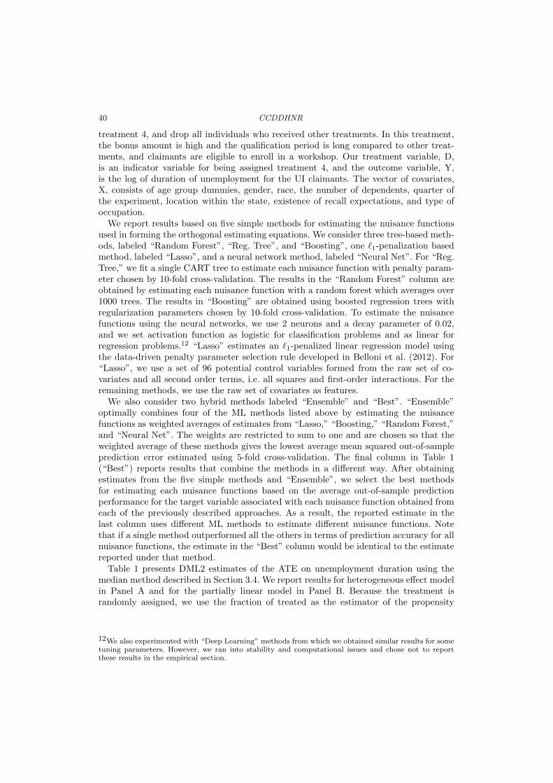
40 CCDDHNR

treatment 4, and drop all individuals who received other treatments. In this treatment,the bonus amount is high and the qualification period is long compared to other treat-ments, and claimants are eligible to enroll in a workshop. Our treatment variable, D,is an indicator variable for being assigned treatment 4, and the outcome variable, Y,is the log of duration of unemployment for the UI claimants. The vector of covariates,X, consists of age group dummies, gender, race, the number of dependents, quarter ofthe experiment, location within the state, existence of recall expectations, and type ofoccupation.

We report results based on five simple methods for estimating the nuisance functionsused in forming the orthogonal estimating equations. We consider three tree-based meth-ods, labeled “Random Forest”, “Reg. Tree”, and “Boosting”, one `1-penalization basedmethod, labeled “Lasso”, and a neural network method, labeled “Neural Net”. For “Reg.Tree,” we fit a single CART tree to estimate each nuisance function with penalty param-eter chosen by 10-fold cross-validation. The results in the “Random Forest” column areobtained by estimating each nuisance function with a random forest which averages over1000 trees. The results in “Boosting” are obtained using boosted regression trees withregularization parameters chosen by 10-fold cross-validation. To estimate the nuisancefunctions using the neural networks, we use 2 neurons and a decay parameter of 0.02,and we set activation function as logistic for classification problems and as linear forregression problems.12 “Lasso” estimates an `1-penalized linear regression model usingthe data-driven penalty parameter selection rule developed in Belloni et al. (2012). For“Lasso”, we use a set of 96 potential control variables formed from the raw set of co-variates and all second order terms, i.e. all squares and first-order interactions. For theremaining methods, we use the raw set of covariates as features.

We also consider two hybrid methods labeled “Ensemble” and “Best”. “Ensemble”optimally combines four of the ML methods listed above by estimating the nuisancefunctions as weighted averages of estimates from “Lasso,” “Boosting,” “Random Forest,”and “Neural Net”. The weights are restricted to sum to one and are chosen so that theweighted average of these methods gives the lowest average mean squared out-of-sampleprediction error estimated using 5-fold cross-validation. The final column in Table 1(“Best”) reports results that combine the methods in a different way. After obtainingestimates from the five simple methods and “Ensemble”, we select the best methodsfor estimating each nuisance functions based on the average out-of-sample predictionperformance for the target variable associated with each nuisance function obtained fromeach of the previously described approaches. As a result, the reported estimate in thelast column uses different ML methods to estimate different nuisance functions. Notethat if a single method outperformed all the others in terms of prediction accuracy for allnuisance functions, the estimate in the “Best” column would be identical to the estimatereported under that method.

Table 1 presents DML2 estimates of the ATE on unemployment duration using themedian method described in Section 3.4. We report results for heterogeneous effect modelin Panel A and for the partially linear model in Panel B. Because the treatment israndomly assigned, we use the fraction of treated as the estimator of the propensity

12We also experimented with “Deep Learning” methods from which we obtained similar results for sometuning parameters. However, we ran into stability and computational issues and chose not to reportthese results in the empirical section.

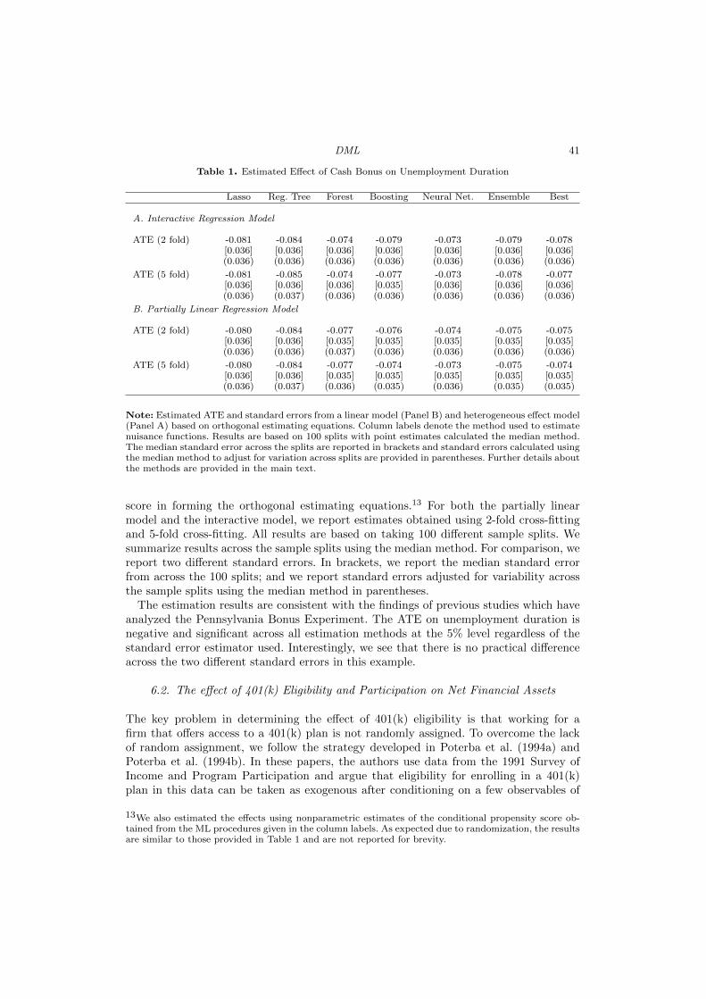
DML 41

Table 1. Estimated Effect of Cash Bonus on Unemployment Duration

Lasso Reg. Tree Forest Boosting Neural Net. Ensemble Best

A. Interactive Regression Model

ATE (2 fold) -0.081 -0.084 -0.074 -0.079 -0.073 -0.079 -0.078[0.036] [0.036] [0.036] [0.036] [0.036] [0.036] [0.036](0.036) (0.036) (0.036) (0.036) (0.036) (0.036) (0.036)

ATE (5 fold) -0.081 -0.085 -0.074 -0.077 -0.073 -0.078 -0.077[0.036] [0.036] [0.036] [0.035] [0.036] [0.036] [0.036](0.036) (0.037) (0.036) (0.036) (0.036) (0.036) (0.036)

B. Partially Linear Regression Model

ATE (2 fold) -0.080 -0.084 -0.077 -0.076 -0.074 -0.075 -0.075[0.036] [0.036] [0.035] [0.035] [0.035] [0.035] [0.035](0.036) (0.036) (0.037) (0.036) (0.036) (0.036) (0.036)

ATE (5 fold) -0.080 -0.084 -0.077 -0.074 -0.073 -0.075 -0.074[0.036] [0.036] [0.035] [0.035] [0.035] [0.035] [0.035](0.036) (0.037) (0.036) (0.035) (0.036) (0.035) (0.035)

Note: Estimated ATE and standard errors from a linear model (Panel B) and heterogeneous effect model(Panel A) based on orthogonal estimating equations. Column labels denote the method used to estimatenuisance functions. Results are based on 100 splits with point estimates calculated the median method.The median standard error across the splits are reported in brackets and standard errors calculated usingthe median method to adjust for variation across splits are provided in parentheses. Further details aboutthe methods are provided in the main text.

score in forming the orthogonal estimating equations.13 For both the partially linearmodel and the interactive model, we report estimates obtained using 2-fold cross-fittingand 5-fold cross-fitting. All results are based on taking 100 different sample splits. Wesummarize results across the sample splits using the median method. For comparison, wereport two different standard errors. In brackets, we report the median standard errorfrom across the 100 splits; and we report standard errors adjusted for variability acrossthe sample splits using the median method in parentheses.

The estimation results are consistent with the findings of previous studies which haveanalyzed the Pennsylvania Bonus Experiment. The ATE on unemployment duration isnegative and significant across all estimation methods at the 5% level regardless of thestandard error estimator used. Interestingly, we see that there is no practical differenceacross the two different standard errors in this example.

6.2. The effect of 401(k) Eligibility and Participation on Net Financial Assets

The key problem in determining the effect of 401(k) eligibility is that working for afirm that offers access to a 401(k) plan is not randomly assigned. To overcome the lackof random assignment, we follow the strategy developed in Poterba et al. (1994a) andPoterba et al. (1994b). In these papers, the authors use data from the 1991 Survey ofIncome and Program Participation and argue that eligibility for enrolling in a 401(k)plan in this data can be taken as exogenous after conditioning on a few observables of

13We also estimated the effects using nonparametric estimates of the conditional propensity score ob-tained from the ML procedures given in the column labels. As expected due to randomization, the resultsare similar to those provided in Table 1 and are not reported for brevity.

42 CCDDHNR

which the most important for their argument is income. The basic idea of their argumentis that, at least around the time 401(k) initially became available, people were unlikelyto be basing their employment decisions on whether an employer offered a 401(k) butwould instead focus on income and other aspects of the job. Following this argument,whether one is eligible for a 401(k) may then be taken as exogenous after appropriatelyconditioning on income and other control variables related to job choice.

A key component of the argument underlying the exogeneity of 401(k) eligibility isthat eligibility may only be taken as exogenous after conditioning on income and othervariables related to job choice that may correlate with whether a firm offers a 401(k).Poterba et al. (1994a) and Poterba et al. (1994b) and many subsequent papers adoptthis argument but control only linearly for a small number of terms. One might wonderwhether such specifications are able to adequately control for income and other relatedconfounds. At the same time, the power to learn about treatment effects decreases as oneallows more flexible models. The principled use of flexible ML tools offers one resolutionto this tension. The results presented below thus complement previous results which relyon the assumption that confounding effects can adequately be controlled for by a smallnumber of variables chosen ex ante by the researcher.

In the example in this paper, we use the same data as in Chernozhukov and Hansen(2004). We use net financial assets - defined as the sum of IRA balances, 401(k) bal-ances, checking accounts, U.S. saving bonds, other interest-earning accounts in banksand other financial institutions, other interest-earning assets (such as bonds held person-ally), stocks, and mutual funds less non-mortgage debt - as the outcome variable, Y , inour analysis. Our treatment variable, D, is an indicator for being eligible to enroll in a401(k) plan. The vector of raw covariates, X, consists of age, income, family size, years ofeducation, a married indicator, a two-earner status indicator, a defined benefit pensionstatus indicator, an IRA participation indicator, and a home ownership indicator.

In Table 2, we report DML2 estimates of ATE of 401(k) eligibility on net financial assetsboth in the partially linear model as in (1.1) and allowing for heterogeneous treatmenteffects using the interactive model outlined in Section 5.1. To reduce the disproportionateimpact of extreme propensity score weights in the interactive model, we trim the propen-sity scores at 0.01 and 0.99. We present two sets of results based on sample-splittingas discussed in Section 3 using 2-fold cross-fitting and 5-fold cross-fitting. As in theprevious section, we consider 100 different sample partitions and summarize the resultsacross different sample splits using the median method. For comparison, we report twodifferent standard errors. In brackets, we report the median standard error from acrossthe 100 splits; and we report standard errors adjusted for variability across the samplesplits using the median method in parentheses. We consider the same methods with thesame tuning choices for estimating the nuisance functions as in the previous example,with one exception, and so do not repeat details for brevity. The one exception is thatwe implement neural networks with 8 neurons and a decay parameter of 0.01 in thisexample.

Turning to the results, it is first worth noting that the estimated ATE of 401(k) eligi-bility on net financial assets is $19,559 with an estimated standard error of 1413 whenno control variables are used. Of course, this number is not a valid estimate of the causaleffect of 401(k) eligibility on financial assets if there are neglected confounding variablesas suggested by Poterba et al. (1994a) and Poterba et al. (1994b). When we turn to theestimates that flexibly account for confounding reported in Table 2, we see that they aresubstantially attenuated relative to this baseline that does not account for confounding,

DML 43

Table 2. Estimated Effect of 401(k) Eligibility on Net Financial Assets

Lasso Reg. Tree Forest Boosting Neural Net. Ensemble Best

A. Interactive Regression Model

ATE (2 fold) 6830 7713 7770 7806 7764 7702 7546[1282] [1208] [1276] [1159] [1328] [1149] [1360](1530) (1271) (1363) (1202) (1468) (1170) (1533)

ATE (5 fold) 7170 7993 8105 7713 7788 7839 7753[1201] [1198] [1242] [1155] [1238] [1134] [1237](1398) (1236) (1299) (1177) (1293) (1148) (1294)

B. Partially Linear Regression Model

ATE (2 fold) 7717 8709 9116 8759 8950 9010 9125[1346] [1363] [1302] [1339] [1335] [1309] [1304](1749) (1427) (1377) (1382) (1408) (1344) (1357)

ATE (5 fold) 8187 8871 9247 9110 9038 9166 9215[1298] [1358] [1295] [1314] [1322] [1299] [1294](1558) (1418) (1328) (1328) (1355) (1310) (1312)

Note: Estimated ATE and standard errors from a linear model (Panel B) and heterogeneous effect model(Panel A) based on orthogonal estimating equations. Column labels denote the method used to estimatenuisance functions. Results are based on 100 splits with point estimates calculated the median method.The median standard error across the splits are reported in brackets and standard errors calculated usingthe median method to adjust for variation across splits are provided in parentheses. Further details aboutthe methods are provided in the main text.

suggesting much smaller causal effects of 401(k) eligibility on financial asset holdings. Itis interesting and reassuring that the results obtained from the different flexible methodsare broadly consistent with each other. This similarity is consistent with the theory thatsuggests that results obtained through the use of orthogonal estimating equations andany sensible method of estimating the necessary nuisance functions should be similar.Finally, it is interesting that these results are also broadly consistent with those reportedin the original work of Poterba et al. (1994a) and Poterba et al. (1994b) which used asimple intuitively motivated functional form, suggesting that this intuitive choice wassufficiently flexible to capture much of the confounding variation in this example.

As a further illustration, we also report the LATE in this example where we take theendogenous treatment variable to be participating in a 401(k) plan. Even after controllingfor features related to job choice, it seems likely that the actual choice of whether toparticipate in an offered plan would be endogenous. Of course, we can use eligibility fora 401(k) plan as an instrument for participation in a 401(k) plan under the conditionsthat were used to justify the exogeneity of eligibility for a 401(k) plan provided above inthe discussion of estimation of the ATE of 401(k) eligibility.

We report DML2 results of estimating the LATE of 401(k) participation using 401(k)eligibility as an instrument in Table 3. We employ the procedure outlined in Section 5.2using the same ML estimators to estimate the quantities used to form the orthogonalestimating equation as we employed to estimate the ATE of 401(k) eligibility outlinedpreviously, so we omit the details for brevity. Looking at the results, we see that the es-timated causal effect of 401(k) participation on net financial assets is uniformly positiveand statistically significant across all of the considered methods. As when looking at theATE of 401(k) eligibility, it is reassuring that the results obtained from the different flex-

44 CCDDHNR

Table 3. Estimated Effect of 401(k) Participation on Net Financial Assets

Lasso Reg. Tree Forest Boosting Neural Net. Ensemble Best

A. Interactive Regression Model

LATE (2 fold) 8978 11073 11384 11329 11094 11119 10952[2192] [1749] [1832] [1666] [1903] [1653] [1657](3014) (1849) (1993) (1718) (2098) (1689) (1699)

LATE (5 fold) 8944 11459 11764 11133 11186 11173 11113[2259] [1717] [1788] [1661] [1795] [1641] [1645](3307) (1786) (1893) (1710) (1890) (1678) (1675)

Note: Estimated LATE based on orthogonal estimating equations. Column labels denote the methodused to estimate nuisance functions. Results are based on 100 splits with point estimates calculated themedian method. The median standard error across the splits are reported in brackets and standard errorscalculated using the median method to adjust for variation across splits are provided in parentheses.Further details about the methods are provided in the main text.

ible methods are broadly consistent with each other. It is also interesting that the resultsbased on flexible ML methods are broadly consistent with, though somewhat attenuatedrelative to, those obtained by applying the same specification for controls as used inPoterba et al. (1994a) and Poterba et al. (1994b) and using a linear IV model whichreturns an estimated effect of participation of $13,102 with estimated standard error of(1922). The mild attenuation may suggest that the simple intuitive control specificationused in the original baseline specification is somewhat too simplistic.

Looking at Tables 2 and 3, there are other interesting observations that can provideuseful insights into understanding the finite sample properties of the DML estimationmethod. First, the standard errors of the estimates obtained using 5-fold cross-fitting arelower than those obtained from 2-fold cross-fitting for all methods across all cases. Thisfact suggests that having more observations in the auxiliary sample may be desirable.Specifically, the 5-fold cross-fitting estimates use more observations to learn the nuisancefunctions than 2-fold cross-fitting and thus likely learn them more precisely. This increasein precision in learning the nuisance functions may then translate into more preciselyestimated parameters of interest. While intuitive, we note that this statement does notseem to be generalizable in that there does not appear to be a general relationshipbetween the number of folds in cross-fitting and the precision of the estimate of theparameter of interest; see the next example. Second, we also see that the standard errorsof the Lasso estimates after adjusting for variation due to sample splitting are noticeablylarger than the standard errors coming from the other ML methods. We believe thatthis is due to the fact that the out-of-sample prediction errors from a linear modeltend to be larger when there is a need to extrapolate. In our framework, if the mainsample includes observations that are outside of the range of the observations in theauxiliary sample, the model has to extrapolate to those observations. The fact that thestandard errors are lower in 5-fold cross-fitting than in 2-fold cross-fitting for the “Lasso”estimations also supports this hypothesis, because the higher number of observations inthe auxiliary sample reduces the degree of extrapolation. We also see that there is anoticeable increase in the standard errors that account for variability due to samplesplitting relative to the simple unadjusted standard errors in this case, though thesedifferences do not qualitatively change the results.

DML 45

6.3. The Effect of Institutions on Economic Growth

To demonstrate DML estimation of partially linear structural equation models with in-strumental variables, we consider estimation of the effect of institutions on aggregateoutput following the work of Acemoglu et al. (2001) (AJR). Estimating the effect ofinstitutions on output is complicated by the clear potential for simultaneity between in-stitutions and output: Specifically, better institutions may lead to higher incomes, buthigher incomes may also lead to the development of better institutions. To help overcomethis simultaneity, AJR use mortality rates for early European settlers as an instrumentfor institution quality. The validity of this instrument hinges on the argument that set-tlers set up better institutions in places where they are more likely to establish long-termsettlements; that where they are likely to settle for the long term is related to settlermortality at the time of initial colonization; and that institutions are highly persistent.The exclusion restriction for the instrumental variable is then motivated by the argu-ment that GDP, while persistent, is unlikely to be strongly influenced by mortality inthe previous century, or earlier, except through institutions.

In their paper, AJR note that their instrumental variable strategy will be invalidatedif other factors are also highly persistent and related to the development of institutionswithin a country and to the country’s GDP. A leading candidate for such a factor, asthey discuss, is geography. AJR address this by assuming that the confounding effect ofgeography is adequately captured by a linear term in distance from the equator and a setof continent dummy variables. Using DML allows us to relax this assumption and replaceit by a weaker assumption that geography can be sufficiently controlled by an unknownfunction of distance from the equator and continent dummies which can be learned byML methods.

We use the same set of 64 country-level observations as AJR. The data set containsmeasurements of GDP, settler morality, an index which measures protection against ex-propriation risk and geographic information. The outcome variable, Y, is the logarithm ofGDP per capita and the endogenous explanatory variable, D, is a measure of the strengthof individual property rights that is used as a proxy for the strength of institutions. Todeal with endogeneity, we use an instrumental variable Z, which is mortality rates forearly European settlers. Our raw set of control variables, X, include distance from theequator and dummy variables for Africa, Asia, North America, and South America.

We report results from applying DML2 following the procedure outlined in Section4.2 in Table 4. The considered ML methods and tuning parameters are the same asthe previous examples except for the Ensemble method, from which we exclude NeuralNetwork since the small sample size causes stability problems in training the NeuralNetwork. We use the raw set of covariates and all second order terms when doing lassoestimation, and we simply use the raw set of covariates in the remaining methods. As inthe previous examples, we consider 100 different sample splits and report the “Median”estimates of the coefficient and two different standard error estimates. In brackets, wereport the median standard error from across the 100 splits; and we report standard errorsadjusted for variability across the sample splits using the median method in parentheses.Finally, we report results from both 2-fold cross-fitting and 5-fold cross-fitting as in theother examples.

In this example, we see uniformly large and positive point estimates across all proce-dures considered. However, the estimated standard errors are also large; so the estimatedeffects are not statistically significant at the 5% level in any case. As in the second exam-

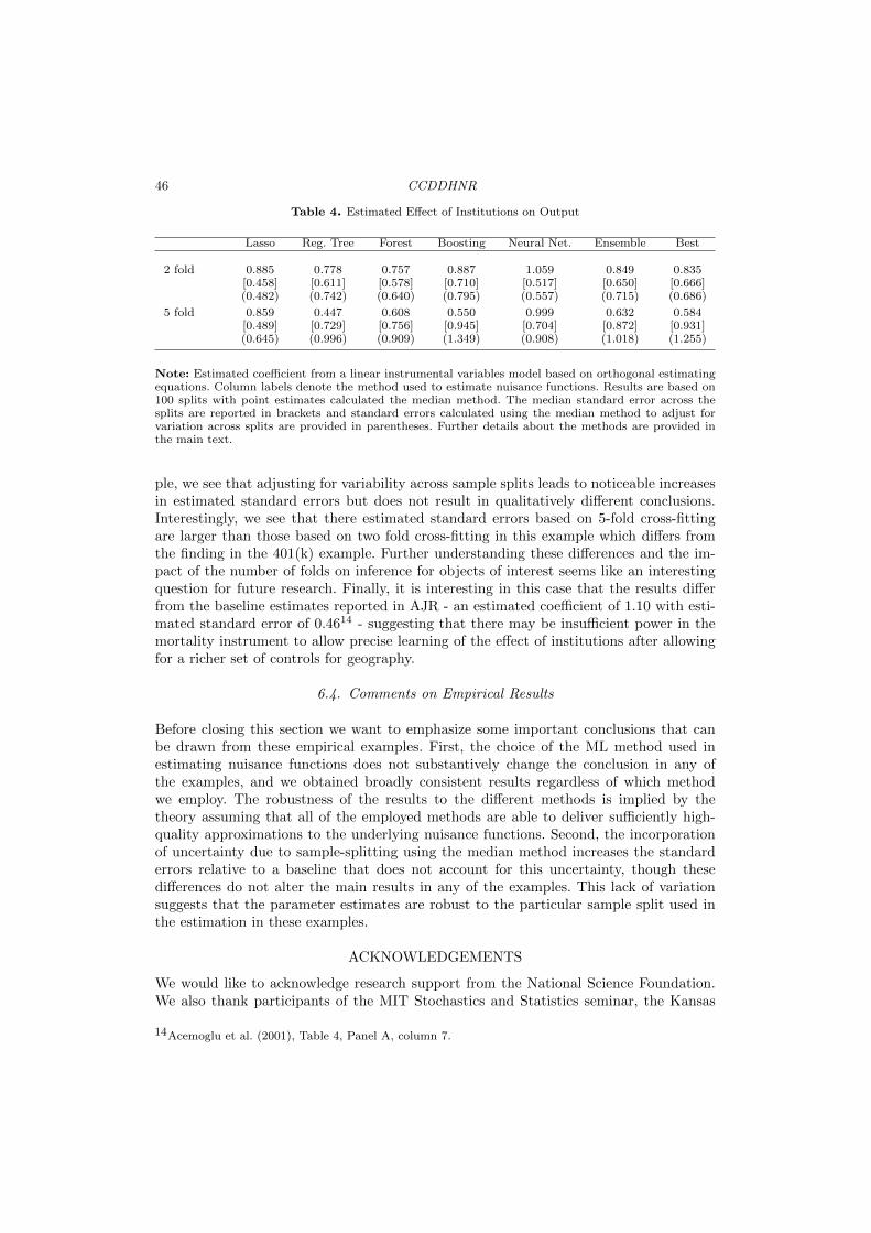
46 CCDDHNR

Table 4. Estimated Effect of Institutions on Output

Lasso Reg. Tree Forest Boosting Neural Net. Ensemble Best

2 fold 0.885 0.778 0.757 0.887 1.059 0.849 0.835[0.458] [0.611] [0.578] [0.710] [0.517] [0.650] [0.666](0.482) (0.742) (0.640) (0.795) (0.557) (0.715) (0.686)

5 fold 0.859 0.447 0.608 0.550 0.999 0.632 0.584[0.489] [0.729] [0.756] [0.945] [0.704] [0.872] [0.931](0.645) (0.996) (0.909) (1.349) (0.908) (1.018) (1.255)

Note: Estimated coefficient from a linear instrumental variables model based on orthogonal estimatingequations. Column labels denote the method used to estimate nuisance functions. Results are based on100 splits with point estimates calculated the median method. The median standard error across thesplits are reported in brackets and standard errors calculated using the median method to adjust forvariation across splits are provided in parentheses. Further details about the methods are provided inthe main text.

ple, we see that adjusting for variability across sample splits leads to noticeable increasesin estimated standard errors but does not result in qualitatively different conclusions.Interestingly, we see that there estimated standard errors based on 5-fold cross-fittingare larger than those based on two fold cross-fitting in this example which differs fromthe finding in the 401(k) example. Further understanding these differences and the im-pact of the number of folds on inference for objects of interest seems like an interestingquestion for future research. Finally, it is interesting in this case that the results differfrom the baseline estimates reported in AJR - an estimated coefficient of 1.10 with esti-mated standard error of 0.4614 - suggesting that there may be insufficient power in themortality instrument to allow precise learning of the effect of institutions after allowingfor a richer set of controls for geography.

6.4. Comments on Empirical Results

Before closing this section we want to emphasize some important conclusions that canbe drawn from these empirical examples. First, the choice of the ML method used inestimating nuisance functions does not substantively change the conclusion in any ofthe examples, and we obtained broadly consistent results regardless of which methodwe employ. The robustness of the results to the different methods is implied by thetheory assuming that all of the employed methods are able to deliver sufficiently high-quality approximations to the underlying nuisance functions. Second, the incorporationof uncertainty due to sample-splitting using the median method increases the standarderrors relative to a baseline that does not account for this uncertainty, though thesedifferences do not alter the main results in any of the examples. This lack of variationsuggests that the parameter estimates are robust to the particular sample split used inthe estimation in these examples.

ACKNOWLEDGEMENTS

We would like to acknowledge research support from the National Science Foundation.We also thank participants of the MIT Stochastics and Statistics seminar, the Kansas

14Acemoglu et al. (2001), Table 4, Panel A, column 7.

DML 47

Econometrics conference, the Royal Economic Society Annual Conference, The HannanLecture at the Australasian Econometric Society meeting, The Econometric Theory lec-ture at the EC2 meetings 2016 in Toulouse, The CORE 50th Anniversary Conference,The Becker-Friedman Institute Conference on Machine Learning and Economics, TheINET conferences at USC on Big Data, the World Congress of Probability and Statistics2016, the Joint Statistical Meetings 2016, the New England Day of Statistics Conference,CEMMAP’s Masterclass on Causal Machine Learning, and St. Gallen’s summer schoolon “Big Data”, for many useful comments and questions. We would like to thank SusanAthey, Peter Aronow, Jin Hahn, Guido Imbens, Mark van der Laan, and Matt Taddyfor constructive comments. We thank Peter Aronow for pointing us to the literature ontargeted learning on which, along with prior works of Neyman, Bickel, and the manyother contributions to semiparametric learning theory, we build.

REFERENCES

Abadie, A. and G. W. Imbens (2006). Large sample properties of matching estimatorsfor average treatment effects. Econometrica 74 (1), 235–267.

Acemoglu, D., S. Johnson, and J. A. Robinson (2001, December). The colonial ori-gins of comparative development: An empirical investigation. American EconomicReview 91 (5), 1369–1401.

Ai, C. and X. Chen (2012). The semiparametric efficiency bound for models of sequentialmoment restrictions containing unknown functions. Journal of Econometrics 170 (2),442–457.

Andrews, D. W. K. (1994a). Asymptotics for semiparametric econometric models viastochastic equicontinuity. Econometrica 62 (1), 43–72.

Andrews, D. W. K. (1994b). Empirical process methods in econometrics. Handbook ofEconometrics, Volume IV, Chapter 37 , 2247–2294.

Angrist, J. D. and A. B. Krueger (1995). Split-sample instrumental variables estimates ofthe return to schooling. Journal of Business and Economic Statistics 13 (2), 225–235.

Athey, S., G. Imbens, and S. Wager (2016). Approximate residual balancing: De-biasedinference of average treatment effects in high-dimensions. arXiv:1604.07125v3 . arXiv,2016.

Ayyagari, R. (2010). Applications of influence functions to semiparametric regressionmodels. Ph.D. Thesis, Harvard School of Public Health, Harvard University.

Belloni, A., D. Chen, V. Chernozhukov, and C. Hansen (2012). Sparse models and meth-ods for optimal instruments with an application to eminent domain. Econometrica 80,2369–2429. ArXiv, 2010.

Belloni, A. and V. Chernozhukov (2011). `1-penalized quantile regression for high di-mensional sparse models. Annals of Statistics 39 (1), 82–130. ArXiv, 2009.

Belloni, A. and V. Chernozhukov (2013). Least squares after model selection in high-dimensional sparse models. Bernoulli 19 (2), 521–547. ArXiv, 2009.

Belloni, A., V. Chernozhukov, I. Fernandez-Val, and C. Hansen (2013). Program evalu-ation with high-dimensional data. arXiv:1311.2645 . arXiv 2013, forthcoming Econo-metrica.

Belloni, A., V. Chernozhukov, and C. Hansen (2010). Lasso methods for gaussian instru-mental variables models. arXiv preprint arXiv:1012.1297 .

Belloni, A., V. Chernozhukov, and C. Hansen (2013). Inference for high-dimensionalsparse econometric models. Advances in Economics and Econometrics. 10th WorldCongress of Econometric Society. August 2010 , III:245–295. ArXiv, 2011.

48 CCDDHNR

Belloni, A., V. Chernozhukov, and C. Hansen (2014). Inference on treatment effects afterselection amongst high-dimensional controls. Review of Economic Studies 81, 608–650.ArXiv, 2011.

Belloni, A., V. Chernozhukov, and K. Kato (2015). Uniform post selection inference forlad regression models and other z-estimators. Biometrika 102, 77–94. ArXiv, 2013.

Belloni, A., V. Chernozhukov, and L. Wang (2011). Square-root-lasso: Pivotal recoveryof sparse signals via conic programming. Biometrika 98 (4), 791–806. Arxiv, 2010.

Belloni, A., V. Chernozhukov, and L. Wang (2014). Pivotal estimation via square-rootlasso in nonparametric regression. Annals of Statistics (arXiv 2011) 42 (2), 757–788.

Belloni, A., V. Chernozhukov, and Y. Wei (2013). Honest confidence regions for logisticregression with a large number of controls. arXiv preprint arXiv:1304.3969 . arXiv2013, forthcoming Journal of Business and Economic Statistics.

Bera, A., G. Montes-Rojas, and W. Sosa-Escudero (2010). General specification testingwith locally misspecified models. Econometric Theory 26, 1838–1845.

Bickel, P. and Y. Ritov (1988). Estimating integrated squared density derivatives.Sankhya A-50, 381–393.

Bickel, P. J. (1982). On adaptive estimation. Annals of Statistics 10 (3), 647–671.Bickel, P. J., C. A. J. Klaassen, Y. Ritov, and J. A. Wellner (1998). Efficient and Adaptive

Estimation for Semiparametric Models. Springer.Bickel, P. J., Y. Ritov, and A. Tsybakov (2009). Simultaneous analysis of Lasso and

Dantzig selector. Annals of Statistics 37 (4), 1705–1732. ArXiv, 2008.Bilias, Y. (2000). Sequential testing of duration data: the case of the pennsylva-

nia’reemployment bonus’ experiment. Journal of Applied Econometrics 15, 575–594.Bilias, Y. and R. Koenker (2002). Quantile regression for duration data: a reappraisal of

the pennsylvania reemployment bonus experiments. Economic Applications of QuantileRegression 2002 , 199–220.

Buhlmann, P. and S. van de Geer (2011). Statistics for High-Dimensional Data. SpringerSeries in Statistics.

Chamberlain, G. (1987). Asymptotic efficiency in estimation with conditional momentrestrictions. Journal of Econometrics 34, 305–334.

Chamberlain, G. (1992). Efficiency bounds for semiparametric regression. Economet-rica 60, 567–596.

Chen, X., O. Linton, and I. van Keilegom (2003). Estimation of semiparametric modelswhen the criterion function is not smooth. Econometrica 71 (5), 1591–1608.

Chen, X. and H. White (1999). Improved rates and asymptotic normality for nonpara-metric neural network estimators. IEEE Transactions on Information Theory 45 (2),682–691.

Chernozhukov, V., D. Chetverikov, and K. Kato (2014). Gaussian approximation ofsuprema of empirical processes. The Annals of Statistics 42 (4), 1564–1597. ArXiv,2012.

Chernozhukov, V., J. Escanciano, H. Ichimura, W. Newey, and J. Robins (2016). Locallyrobust semiparametric estimation. Working paper.

Chernozhukov, V. and C. Hansen (2004). The effects of 401 (k) participation on thewealth distribution: an instrumental quantile regression analysis. Review of Economicsand statistics 86 (3), 735–751.

Chernozhukov, V., C. Hansen, and M. Spindler (2015a). Post-selection and post-regularization inference in linear models with very many controls and instruments.Americal Economic Review: Papers and Proceedings 105, 486–490.

DML 49

Chernozhukov, V., C. Hansen, and M. Spindler (2015b). Valid post-selection and post-regularization inference: An elementary, general approach. Annual Review of Eco-nomics 7, 649–688.

DasGupta, A. (2008). Asymptotic Theory of Statistics and Probability. Springer Textsin Statistics.

Fan, J., S. Guo, and K. Yu (2012). Variance estimation using refitted cross-validation inultrahigh dimensional regression. Journal of the Royal Statistical Society, Series B 74,37–65.

Farrell, M. (2015). Robust inference on average treatment effects with possibly morecovariates than observations. Journal of Econometrics 174 (2), 1–23.

Ferguson, T. (1967). Mathematical Statistics: A Decision Theoretic Approach. AcademicPress.

Frolich, M. (2007). Nonparametric iv estimation of local average treatment effects withcovariates. Journal of Econometrics, 3575.

Gautier, E. and A. Tsybakov (2011). High-dimensional instrumental variables regressionand confidence sets. Working paper.

Hahn, J. (1998). On the role of the propensity score in efficient semiparametric estimationof average treatment effects. Econometrica 1998, 315–331.

Hansen, L. (1982). Large sample properties of generalized method of moments estimators.Econometrica 50, 1029–1054.

Hasminskii, R. and I. Ibragimov (1978). On the nonparametric estimation of functionals.Proceedings of the 2nd Prague Symposium on Asymptotic Statistics, 41–51.

Hirano, K., G. W. Imbens, and G. Ridder (2003). Efficient estimation of average treat-ment effects using the estimated propensity score. Econometrica 71, 1161–1189.

Hubbard, A. E., S. Kherad-Pajouh, and M. J. van der Laan (2016). Statistical inferencefor data adaptive target parameters. International Journal of Biostatistics 12 (1), 3–19.

Ibragimov, I. A. and R. Z. Hasminskii (1981). Statistical Estimation: Asymptotic Theory.Springer-Verlag, New York.

Ichimura, H. and W. Newey (2015). The influence function of semiparametric estimators.Working paper.

Imai, K. and M. Ratkovic (2013). Estimating treatment effect heterogeneity in random-ized program evaluation. Annals of Applied Statistics 7 (1), 443–470.

Imbens, G. and J. Angrist (1994). Identification and estimation of local average treatmenteffects. Econometrica, 467475.

Imbens, G. W. and D. B. Rubin (2015). Causal Inference for Statistics, Social, andBiomedical Sciences: An Introduction. Cambridge University Press.

Javanmard, A. and A. Montanari (2014a). Confidence intervals and hypothesis testingfor high-dimensional regression. Journal of Machine Learning Research 15, 2869–2909.

Javanmard, A. and A. Montanari (2014b). Hypothesis testing in high-dimensional regres-sion under the gaussian random design model: asymptotic theory. IEEE Transactionson Information Theory 60, 6522–6554. ArXiv, 2013.

Kozbur, D. (2016). Testing-based forward model selection. arXiv:1512.02666 . arXiv,2015.

Lee, L. (2005). A c(α)-type gradient test in the gmm approach. Working paper.Levit, B. Y. (1975). On the efficiency of a class of nonparametric estimates. Theory of

Probability and Its Applications 20, 723–740.Linton, O. (1996). Edgeworth approximation for MINPIN estimators in semiparametric

regression models. Econometric Theory 12 (1), 30–60.

50 CCDDHNR

Luedtke, A. R. and M. J. van der Laan (2016). Optimal individualized treatments inresource-limited settings. The international journal of biostatistics 12 (1), 283–303.

Luo, Y. and M. Spindler (2016). High-dimensional l2 boosting: Rate of convergence.arXiv:1602.08927 . arXiv, 2016.

Nevelson, M. (1977). One informational lower bound. Problemy Peredachi Informatsii ,26–31.

Newey, W. (1990). Semiparametric efficiency bounds. Journal of Applied Economet-rics 5 (2), 99–135.

Newey, W. (1994). The asymptotic variance of semiparametric estimators. Economet-rica 62 (6), 1349–1382.

Newey, W. K., F. Hsieh, and J. Robins (1998). Undersmoothing and biascorrected functional estimation. Working paper, MIT Economics Dept.,http://economics.mit.edu/files/11219.

Newey, W. K., F. Hsieh, and J. M. Robins (2004). Twicing kernels and a small biasproperty of semiparametric estimators. Econometrica 72 (3), 947–962.

Neyman, J. (1959). Optimal asymptotic tests of composite statistical hypotheses. Prob-ability and statistics 57, 213.

Neyman, J. (1979). c(α) tests and their use. Sankhya, 1–21.Poterba, J. M., S. F. Venti, and D. A. Wise (1994a). 401(k) plans and tax-deferred

savings. In D. Wise (Ed.), Studies in the Economics of Aging, pp. 105–142. Chicago:University of Chicago Press.

Poterba, J. M., S. F. Venti, and D. A. Wise (1994b). Do 401(k) contributions crowd outother personal saving? Journal of Public Economics 58, 1–32.

Robins, J., L. Li, R. Mukherjee, E. Tchetgen, and A. van der Vaart (2017). Minimaxestimation of a functional on a structured high dimensional model. Annals of Statistics,forthcoming .

Robins, J., L. Li, E. Tchetgen, A. van der Vaart, et al. (2008). Higher order influencefunctions and minimax estimation of nonlinear functionals. In Probability and Statis-tics: Essays in Honor of David A. Freedman, pp. 335–421. Institute of MathematicalStatistics.

Robins, J. and A. Rotnitzky (1995). Semiparametric efficiency in multivariate regressionmodels with missing data. J. Amer. Statist. Assoc 90 (429), 122–129.

Robins, J., P. Zhang, R. Ayyagari, R. Logan, E. Tchetgen, L. Li, A. Lumley, andA. van der Vaart (2013). New statistical approaches to semiparametric regressionwith application to air pollution research. Research Report Health Eff Inst.

Robinson, P. M. (1988). Root-N -consistent semiparametric regression. Economet-rica 56 (4), 931–954.

Rosenbaum, P. R. and D. B. Rubin (1983). The central role of the propensity score inobservational studies for causal effects. Biometrika 70 (1), 41–55.

Scharfstein, D. O., A. Rotnitzky, and J. M. Robins (1999). Rejoinder to ”adjustingfor non-ignorable drop-out using semiparametric non-response models. Journal of theAmerican Statistical Association 94 (448), 1135–1146.

Schick, A. (1986). On asymptotically efficient estimation in semiparametric models.Annals of Statistics 14, 1139–1151.

Severini, T. A. and W. H. Wong (1992). Profile likelihood and conditionally parametricmodels. The Annals of statistics, 1768–1802.

Toth, B. and M. J. van der Laan (2016). Tmle for marginal structural models based onan instrument. U.C. Berkeley Division of Biostatistics Working Paper Series. WorkingPaper 350.

DML 51

van de Geer, S., P. Buhlmann, Y. Ritov, and R. Dezeure (2014). On asymptotically opti-mal confidence regions and tests for high-dimensional models. Annals of Statistics 42,1166–1202. ArXiv, 2013.

van der Laan, M. and D. Rubin (2006). Targeted maximum likelihood learning. ucberkeley division of biostatistics working paper series.

van der Laan, M. J. (2015). A generally efficient targeted minimum loss based estimator.

van der Laan, M. J., E. C. Polley, and A. E. Hubbard (2007). Super learner. StatisticalApplications in Genetics and Molecular Biology 6 (1). Retrieved 24 Feb. 2017, fromdoi:10.2202/1544-6115.1309.

van der Laan, M. J. and S. Rose (2011). Targeted Learning: Causal Inference for Obser-vational and Experimental Data. Springer.

van der Vaart, A. W. (1991). On differentiable functionals. Annals of Statistics 19 (1),178–204.

van der Vaart, A. W. (1998). Asymptotic Statistics. Cambridge University Press.

Wager, S. and G. Walther (2016). Adaptive concentration of regression trees, with ap-plication to random forests. arXiv:1503.06388 . arXiv, 2015.

Wooldridge, J. (1991). Specification testing and quasi-maximum-likelihood estimation.Journal of Econometrics 48, 29–55.

Zhang, C. and S. Zhang (2014). Confidence intervals for low-dimensional parameterswith high-dimensional data. J. R. Statist. Soc. B 76, 217–242. ArXiv, 2012.

Zheng, W., Z. Luo, and M. J. van der Laan (2016). Marginal structural models withcounterfactual effect modifiers. U.C. Berkeley Division of Biostatistics Working PaperSeries. Working Paper 348.

Zheng, W. and M. J. van der Laan (2011). Cross-validated targeted minimum-loss-basedestimation. In Targeted Learning, pp. 459–474. Springer.

APPENDIX: PROOFS OF RESULTS

In this appendix, we use C to denote a strictly positive constant that is independentof n and P ∈ PN . The value of C may change at each appearance. Also, the notationaN . bN means that aN 6 CbN for all n and some C. The notation aN & bN means thatbN . aN . Moreover, the notation aN = o(1) means that there exists a sequence (bN )n>1

of positive numbers such that (i) |aN | 6 bN for all n, (ii) bN is independent of P ∈ PNfor all n, and (iii) bN → 0 as n→∞. Finally, the notation aN = OP (bN ) means that forall ε > 0, there exists C such that PP (aN > CbN ) 6 1− ε for all n. Using this notationallows us to avoid repeating “uniformly over P ∈ PN” many times in the proofs.

Define the empirical process Gn(ψ(W )) as a linear operator acting on measurablefunctions ψ :W → R such that ‖ψ‖P,2 <∞ via,

Gn(ψ(W )) := Gn,I(ψ(W )) :=1√n

∑i∈I

ψ(Wi)−∫ψ(w)dP (w).

Analogously, we defined the empirical expectation as:

En(ψ(W )) := En,I(ψ(W )) :=1

n

∑i∈I

ψ(Wi).

52 CCDDHNR

A.5. Useful Lemmas

The following lemma is useful particularly in the sample-splitting contexts.

Lemma 6.1. (Conditional Convergence Implies Unconditional) Let Xm andYm be sequences of random vectors. (i) If for εm → 0, P(‖Xm‖ > εm | Ym) →P 0,then P(‖Xm‖ > εm) → 0. In particular, this occurs if E[‖Xm‖q/εqm | Ym] →P 0 forsome q > 1, by Markov’s inequality. (ii) Let Am be a sequence of positive constants. If‖Xm‖ = OP (Am) conditional on Ym, namely, that for any `m →∞, P(‖Xm‖ > `mAm |Ym) →P 0, then ‖Xm‖ = OP (Am) unconditionally, namely, that for any `m → ∞,P(‖Xm‖ > `mAm)→ 0.

Proof. Part (i). For any ε > 0 P(‖Xm‖ > εm) 6 E[P(‖Xm‖ > εm | Ym)] → 0, since thesequence P(‖Xm‖ > εm | Ym) is uniformly integrable. To show the second part notethat P(‖Xm‖ > εm | Ym) 6 E[‖Xm‖q/εqm | Ym] ∨ 1 →P 0 by Markov’s inequality. Part(ii). This follows from Part (i).

Let (Wi)ni=1 be a sequence of independent copies of a random element W taking values

in a measurable space (W,AW) according to a probability law P . Let F be a set ofsuitably measurable functions f : W → R, equipped with a measurable envelope F : W →R.

Lemma 6.2. (Maximal Inequality, Chernozhukov et al. (2014)) Work with thesetup above. Suppose that F > supf∈F |f | is a measurable envelope for F with ‖F‖P,q <∞ for some q > 2. Let M = maxi6n F (Wi) and σ2 > 0 be any positive constant suchthat supf∈F ‖f‖2P,2 6 σ2 6 ‖F‖2P,2. Suppose that there exist constants a > e and v > 1such that

log supQN(ε‖F‖Q,2,F , ‖ · ‖Q,2) 6 v log(a/ε), 0 < ε 6 1.

Then

EP [‖Gn‖F ] 6 K

(√vσ2 log

(a‖F‖P,2

σ

)+v‖M‖P,2√

nlog

(a‖F‖P,2

σ

)),

where K is an absolute constant. Moreover, for every t > 1, with probability > 1− t−q/2,

‖Gn‖F 6 (1+α)EP [‖Gn‖F ]+K(q)[(σ+n−1/2‖M‖P,q)

√t+α−1n−1/2‖M‖P,2t

], ∀α > 0,

where K(q) > 0 is a constant depending only on q. In particular, setting a > n andt = log n, with probability > 1− c(log n)−1,

‖Gn‖F 6 K(q, c)

(σ

√v log

(a‖F‖P,2

σ

)+v‖M‖P,q√

nlog

(a‖F‖P,2

σ

)), (A.1)

where ‖M‖P,q 6 n1/q‖F‖P,q and K(q, c) > 0 is a constant depending only on q and c.

A.6. Proof of Lemma 2.2

The proof follows similarly to that of Lemma 2.1, except that now we have to verify(2.12) intead of (2.11). To do so, take any β ∈ B such that ‖β − β0‖∗q 6 λN/rN and any

DML 53

dθ × dβ matrix µ. Denote η = (β′, vec(µ)′)′. Then∥∥∥∂ηEPψ(W, θ0, η0)[η − η0]∥∥∥ =

∥∥∥(Jθβ − µ0Jββ)(β − β0)∥∥∥

6 ‖Jθβ − µ0Jββ‖q × ‖β − β0‖∗q 6 rn × (λN/rN ) = λN .

This completes the proof of the lemma.

A.7. Proof of Lemma 2.3

The proof is similar to that of Lemma 2.1, except that now we have

∂η′EPψ(W, θ0, η0) = [µ0Gβ ,EPm(W, θ0, β0)′ ⊗ Idθ×dθ ] = 0,

where Idθ×dθ is the dθ × dθ identity matrix and ⊗ is the Kronecker product.

A.8. Proof of Lemma 2.4

The proof follows similarly to that of Lemma 2.2, except that now for any β ∈ B suchthat ‖β − β0‖1 6 λN/rN , any dθ × k matrix µ, and η = (β′, vec(µ)′)′, we have∥∥∥∂ηEPψ(W, θ0, η0)[η − η0]

∥∥∥ = ‖µ0Gβ(β − β0)‖

6 ‖A′Ω−1/2L− γ0L′L‖∞ × ‖β − β0‖1

6 rn × (λN/rN ) = λN .

This completes the proof of the lemma.

A.9. Proof of Lemma 2.5

Take any η ∈ T , and consider the function

Q(W ; θ, r) := `(W ; θ, η0(θ) + r(η(θ)− η0(θ))), θ ∈ Θ, r ∈ [0, 1].

Then

ψ(W ; θ, η0 + r(η − η0)) = ∂θQ(W ; θ, r),

and so

∂rEP [ψ(W ; θ, η0 + r(η − η0))] = ∂rEP [∂θQ(W ; θ, r)]

= ∂r∂θEP [Q(W ; θ, r)] = ∂θ∂rEP [Q(W ; θ, r)] (A.2)

= ∂θ∂rEP [`(W ; θ, η0(θ) + r(η(θ)− η0(θ)))].

Hence,

∂rEP [ψ(W ; θ, η0 + r(η − η0))]∣∣∣r=0

= 0

since

∂rEP [`(W ; θ, η0(θ) + r(η(θ)− η0(θ)))]∣∣∣r=0

= 0, for all θ ∈ Θ,

as η0(θ) = βθ solves the optimization problem

maxβ∈B

EP [`(W ; θ, β)], for all θ ∈ Θ.

Here the regularity conditions are needed to make sure that we can interchange EP and∂θ and also ∂θ and ∂r in (A.2). This completes the proof of the lemma.

54 CCDDHNR

A.10. Proof of Lemma 2.6

First, we demonstrate that µ0 ∈ L1(R; Rdθ×dm). Indeed,

EP [‖µ0(R)‖] 6 EP

[‖A(R)′Ω(R)−1‖

]+ EP

[‖G(Z)Γ(R)Ω(R)−1‖

]6 EP

[‖A(R)‖ × ‖Ω(R)‖−1

]+ EP

[‖G(Z)‖ × ‖Γ(R)‖ × ‖Ω(R)‖−1

]6(

EP [‖A(R)‖2]× EP [‖Ω(R)‖−2])1/2

+(

EP

[‖G(Z)‖2 × ‖Γ(R)‖2

]× EP [‖Ω(R)‖−2]

)1/2

,

which is finite by assumptions of the lemma since

EP

[‖G(Z)‖2 × ‖Γ(R)‖2

]6(

EP [‖G(Z)‖4]× EP [Γ(R)‖4])1/2

<∞.

Next, we demonstrate that

EP [‖ψ(W, θ0, η)‖] <∞ for all η ∈ T.

Indeed, for all η ∈ T , there exist µ ∈ L1(R; Rdθ×dm) and h ∈ H such that η = (µ, h),and so

EP [‖ψ(W, θ0, η)‖] = EP [‖µ(X)m(W, θ0, h(Z))‖]

6 EP

[‖µ(R)‖ × ‖m(W, θ0, h(Z))‖

]= EP

[‖µ(R)‖ × EP [‖m(W, θ0, h(Z)) | R]

]6 ChE[‖µ(R)‖],

which is finite by assumptions of the lemma. Further, (2.9) holds because

EP [ψ(W, θ0, η0)] = EP

[µ0(R)m(W, θ0, h0(Z))

]= EP

[µ0(R)EP [m(W, θ0, h0(Z)) | R]

]= 0, (A.3)

where the last equality follows from (2.30).Finally, we demonstrate that (2.11) holds. To do so, take any η = (µ, h) ∈ TN = T .

Then

EP [ψ(W, θ0, η0 + r(η − η0)]

= EP

[(µ0(R) + r(µ(R)− µ0(R)))m(W, θ0, h0(Z) + r(h(Z)− h0(Z)))

],

and so

∂ηEPψ(W, θ0, η0)[η − η0] = I1 + I2,

where

I1 = EP

[(µ(R)− µ0(R))m(W, θ0, h0(Z)

],

I2 = EP

[µ0(R)∂v′m(W, θ0, v)|v=h0(Z)(h(Z)− h0(Z))

].

DML 55

Here I1 = 0 by the same argument as that in (A.3) and I2 = 0 because

I2 = EP

[µ0(R)EP [∂v′m(W, θ0, v)|v=h0(Z) | X](h(Z)− h0(Z))

]= EP

[µ0(R)Γ(X)(h(Z)− h0(Z))

]= EP

[EP [µ0(R)Γ(R) | Z](h(Z)− h0(Z))

]= 0

since

EP [µ0(R)Γ(X) | Z] = EP [A(R)′Ω(R)−1Γ(R) | Z]− EP [G(Z)Γ(R)′Ω(R)−1Γ(R) | Z]

= EP [A(R)′Ω(R)−1Γ(R) | Z]−G(Z)EP [Γ(R)′Ω(R)−1Γ(R) | Z]

= EP [A(R)′Ω(R)−1Γ(R) | Z]− EP [A(R)′Ω(R)−1Γ(R) | Z]

×(

EP [Γ(R)′Ω(R)−1Γ(R) | Z])−1

× EP [Γ(R)′Ω(R)−1Γ(R) | Z]

= EP [A(R)′Ω(R)−1Γ(R) | Z]− EP [A(R)′Ω(R)−1Γ(R) | Z] = 0.

This completes the proof of the lemma.

A.11. Proof of Theorem 3.1 (DML2 case)

To start with, note that (3.48) follows immediately from the assumptions. Hence, itsuffices to show that (3.47) holds uniformly over P ∈ PN .

Fix any sequence PNN>1 such that PN ∈ PN for all N > 1. Since this sequence ischosen arbitrarily, to show that (3.47) holds uniformly over P ∈ PN , it suffices to showthat

√Nσ−1(θ0 − θ0) =

1√N

N∑i=1

ψ(Wi) +OPN (ρN ) ; N(0, Id). (A.4)

To do so, we proceed in 5 steps. Step 1 shows the main argument, and Steps 2–5 presentauxiliary calculations. In the proof, it will be convenient to denote by EN the eventthat η0,k ∈ TN for all k ∈ [K]. Note that by Assumption 3.2 and the union bound,PPN (EN ) > 1−K∆n = 1− o(1) since ∆n = o(1).

Step 1. Denote

J0 :=1

K

K∑k=1

En,k[ψa(W ; η0,k)], RN,1 := J0 − J0,

RN,2 :=1

K

K∑k=1

En,k[ψ(W ; θ0, η0,k)]− 1

N

N∑i=1

ψ(Wi; θ0, η0).

In Steps 2, 3, 4, and 5 below, we will show that

‖RN,1‖ = OPN (N−1/2 + rN ), (A.5)

‖RN,2‖ = OPN (N−1/2r′N + λN + λ′N ), (A.6)

‖N−1/2∑Ni=1 ψ(Wi; θ0, η0)‖ = OPN (1), (A.7)

‖σ−1‖ = OPN (1), (A.8)

respectively. Since N−1/2 + rN 6 ρN = o(1) and all singular values of J0 are boundedbelow from zero by Assumption 3.1, it follows from (A.5) that with PN -probability 1−

56 CCDDHNR

o(1), all singular values of J0 are bounded below from zero as well. Therefore, with thesame PN -probability,

θ0 = −J−10

1

K

K∑k=1

En,k[ψb(W ; η0,k)]

and

√N(θ0 − θ0) = −

√NJ−1

0

( 1

K

K∑k=1

En,k[ψb(W ; η0,k)] + J0θ0

)= −√NJ−1

0

1

K

K∑k=1

En,k[ψ(W ; θ0, η0,k)]

= −(J0 +RN,1

)−1

×( 1√

N

N∑i=1

ψ(Wi; θ0, η0) +√NRN,2

). (A.9)

In addition, given that

(J0 +RN,1)−1 − J−10 = (J0 +RN,1)−1(J0 − (J0 +RN,1))J−1

0

= −(J0 +RN,1)−1RN,1J−10 ,

it follows from (A.5) that

‖(J0 +RN,1)−1 − J−10 ‖ 6 ‖(J0 +RN,1)−1‖ × ‖RN,1‖ × ‖J−1

0 ‖= OPN (1)OPN (N−1/2 + rN )OPN (1) = OPN (N−1/2 + rN ). (A.10)

Moreover, since r′N +√N(λN + λ′N ) 6 ρN = o(1), it follows from (A.6) and (A.7) that∥∥∥ 1√

N

N∑i=1

ψ(Wi; θ0, η0) +√NRN,2

∥∥∥ 6 ∥∥∥ 1√N

N∑i=1

ψ(Wi; θ0, η0)∥∥∥+

∥∥∥√NRN,2∥∥∥= OPN (1) + oPN (1) = OPN (1). (A.11)

Combining (A.10) and (A.11) gives∥∥∥((J0 +RN,1)−1 − J−10

)×( 1√

N

N∑i=1

ψ(Wi; θ0, η0) +√NRN,2

)∥∥∥6∥∥∥(J0 +RN,1)−1 − J−1

0

∥∥∥× ∥∥∥ 1√N

N∑i=1

ψ(Wi; θ0, η0) +√NRN,2

∥∥∥ = OPN (N−1/2 + rN ).

Now, substituting the last bound into (A.9) yields

√N(θ0 − θ0) = −J−1

0 ×( 1√

N

N∑i=1

ψ(Wi; θ0, η0) +√NRN,2

)+OPN (N−1/2 + rN )

= −J−10 × 1√

N

N∑i=1

ψ(Wi; θ0, η0) +OPN (ρN ),

where in the second line we used (A.6) and the definition of ρN . Combining this with

DML 57

(A.8) gives

√Nσ−1(θ0 − θ0) =

1√N

N∑i=1

ψ(Wi) +OPN (ρN ) (A.12)

by the definition of ψ given in the statement of the theorem. In turn, since ρN = o(1),combining (A.12) with the Lindeberg-Feller CLT and the Cramer-Wold device yields(A.4). To complete the proof of the theorem, it remains to establish the bounds (A.5)–(A.8). We do so in four steps below.

Step 2. Here we establish (A.5). Since K is a fixed integer, which is independent of N ,it suffices to show that for any k ∈ [K],∥∥∥En,k[ψa(W ; η0,k)]− EPN [ψa(W ; η0)]

∥∥∥ = OPN (N−1/2 + rN ). (A.13)

To do so, fix any k ∈ [K] and observe that by the triangle inequality,∥∥∥En,k[ψa(W ; η0,k)]− EPN [ψa(W ; η0)]∥∥∥ 6 I1,k + I2,k, (A.14)

where

I1,k :=∥∥∥En,k[ψa(W ; η0,k)]− EPN [ψa(W ; η0,k) | (Wi)i∈Ick ]

∥∥∥,I2,k :=

∥∥∥EPN [ψa(W ; η0,k) | (Wi)i∈Ick ]− EPN [ψa(W ; η0)]∥∥∥.

To bound I2,k, note that on the event EN , which holds with PN -probability 1− o(1),

I2,k 6 supη∈TN

∥∥∥EPN [ψa(W ; η)]− EPN [ψa(W ; η0)]∥∥∥ = rN ,

and so I2,k = OPN (rN ). To bound I1,k, note that conditional on (Wi)i∈Ick , the estimatorη0,k is non-stochastic, and so on the event EN ,

EPN [I21,k | (Wi)i∈Ick ] 6 n−1EPN [‖ψa(W ; η0,k)‖2 | (Wi)i∈Ick ]

6 supη∈TN

n−1EPN [‖ψa(W ; η)‖2] 6 c21/n,

where the last inequality holds by Assumption 3.2. Hence, I1,k = OPN (N−1/2) by Lemma6.1 in the Appendix. Combining the bounds I1,k = OPN (N−1/2) and I2,k = OPN (rN )with (A.14) gives (A.13).

Step 3. Here we establish (A.6). This is the step where we invoke the Neyman orthog-onality (or near-orthogonality) condition. Again, since K is a fixed integer, which isindependent of N , it suffices to show that for any k ∈ [K],

En,k[ψ(W ; θ0, η0,k)]− 1

n

∑i∈Ik

ψ(Wi; θ0, η0) = OPN (N−1/2r′N + λN + λ′N ). (A.15)

To do so, fix any k ∈ [K] and introduce the following additional empirical process nota-tion:

Gn,k[φ(W )] =1√n

∑i∈Ik

(φ(Wi)−

∫φ(w)dPN

),

58 CCDDHNR

where φ is any PN -integrable function onW. Then observe that by the triangle inequality,∥∥∥En,k[ψ(W ; θ0, η0,k)]− 1

n

∑i∈Ik

ψ(Wi; θ0, η0)∥∥∥ 6 I3,k + I4,k√

n, (A.16)

where

I3,k :=∥∥∥Gn,k[ψ(W ; θ0, η0,k)]−Gn,k[ψ(W ; θ0, η0)]

∥∥∥,I4,k :=

√n∥∥∥EPN [ψ(W ; θ0, η0,k) | (Wi)i∈Ick ]− EPN [ψ(W ; θ0, η0)]

∥∥∥.To bound I3,k, note that, as above, conditional on (Wi)i∈Ick , the estimator η0,k is non-stochastic, and so on the event EN ,

EPN [I23,k | (Wi)i∈Ick ] = EPN

[‖ψ(W ; θ0, η0,k)− ψ(W ; θ0, η0)‖2 | (Wi)i∈Ick

]6 supη∈TN

EPN

[‖ψ(W ; θ0, η)− ψ(W ; θ0, η0)‖2 | (Wi)i∈Ick

]6 supη∈TN

EPN

[‖ψ(W ; θ0, η)− ψ(W ; θ0, η0)‖2

]= (r′N )2

by the definition of r′N in Assumption 3.2. Hence, I3,k = OPN (r′N ) by Lemma 6.1 in theAppendix. To bound I4,k, introduce the function

fk(r) := EPN [ψ(W ; θ0, η0 + r(η0,k − η0)) | (Wi)i∈Ick ]− EPN [ψ(W ; θ0, η0)], r ∈ [0, 1].

Then, by Taylor’s expansion,

fk(1) = fk(0) + f ′k(0) + f ′′k (r)/2, for some r ∈ (0, 1).

But ‖fk(0)‖ = 0 since

EPN [ψ(W ; θ0, η0) | (Wi)i∈Ick ] = EPN [ψ(W ; θ0, η0)].

In addition, on the event EN , by the Neyman λN near-orthogonality condition imposedin Assumption 3.1,

‖f ′k(0)‖ =∥∥∥∂ηEPNψ(W ; θ0, η0)[η0,k − η0]

∥∥∥ 6 λN .Moreover, on the event EN ,

‖f ′′k (r)‖ 6 supr∈(0,1)

‖f ′′k (r)‖ 6 λ′N

by the definition λ′N in Assumption 3.2. Hence,

I4,k =√n‖fk(1)‖ = OPN (

√n(λN + λ′N )).

Combining the bounds on I3,k and I4,k with (A.16) and using the fact that n−1 =O(N−1) gives (A.15).

Step 4. To establish (A.7), note that

EPN

[∥∥∥ 1√N

N∑i=1

ψ(Wi; θ0, η0)∥∥∥2]

= EPN

[‖ψ(W ; θ0, η0)‖2

]6 c21

by Assumption 3.2. Combining this with Markov’s inequality gives (A.7).

DML 59

Step 5. Here we establish (A.8). Note that all eigenvalues of the matrix

σ2 = J−10 EP [ψ(W ; θ0, η0)ψ(W ; θ0, η0)′](J−1

0 )′

are bounded from below by c0/c21 since all singular values of J0 are bounded from above

by c1 by Assumption 3.1 and all eigenvalues of EP [ψ(W ; θ0, η0)ψ(W ; θ0, η0)′] are boundedfrom below by c0 by Assumption 3.2. Hence, given that ‖σ−1‖ is the largest eigenvalueof σ−1, it follows that ‖σ−1‖ = c1/

√c0. This gives (A.8) and completes the proof of the

theorem.

A.12. Proof of Theorem 3.1 (DML1 case)

As in the case of the DML2 version, note that (3.48) follows immediately from theassumptions, and so it suffices to show that (3.47) holds uniformly over P ∈ PN .

Fix any sequence PNN>1 such that PN ∈ PN for all N > 1. Since this sequence ischosen arbitrarily, to show that (3.47) holds uniformly over P ∈ PN , it suffices to showthat

√Nσ−1(θ0 − θ0) =

1√N

N∑i=1

ψ(Wi) +OPN (ρN ) ; N(0, Id). (A.17)

To do so, for all k ∈ [K], denote

J0,k := En,k[ψa(W ; η0,k)], RN,1,k := J0,k − J0,

RN,2,k := En,k[ψ(W ; θ0, η0,k)]− 1

n

∑i∈Ik

ψ(Wi; θ0, η0).

Since K is a fixed integer, which is independent of n, it follows by the same argumentsas those in Steps 2–5 in Section A.11 that

maxk∈[K]

‖RN,1,k‖ = OPN (N−1/2 + rN ), (A.18)

maxk∈[K]

‖RN,2,k‖ = OPN (N−1/2r′N + λN + λ′N ), (A.19)

maxk∈[K]

‖n−1/2∑i∈Ik ψ(Wi; θ0, η0)‖ = OPN (1), (A.20)

‖σ−1‖ = OPN (1). (A.21)

Since N−1/2 + rN 6 ρN = o(1) and all singular values of J0 are bounded below fromzero by Assumption 3.1, it follows from (A.18) that for all k ∈ [K], with PN -probability

1 − o(1), all singular values of J0,k are bounded below from zero, and so with the samePN -probability,

θ0,k = −J−10,kEn,k[ψb(W ; η0,k)].

Hence, by the same arguments as those in Step 1 in Section A.11, it follows from thebounds (A.18)–(A.21) that for all k ∈ [K],

√nσ−1(θ0,k − θ0) =

1√n

∑i∈Ik

ψ(Wi) +OPN (ρN ).

60 CCDDHNR

Therefore,

√Nσ−1(θ0 − θ0) =

√Nσ−1

( 1

K

K∑k=1

θ0,k − θ0

)=

1√N

N∑i=1

ψ(Wi) +OPN (ρN ). (A.22)

In turn, since ρN = o(1), combining (A.22) with the Lindeberg-Feller CLT and theCramer-Wold device yields (A.17) and completes the proof of the theorem.

A.13. Proof of Theorem 3.2.

In this proof, all bounds hold uniformly in P ∈ PN for N > 3, and we do not repeat thisqualification throughout. Also, the second asserted claim follows immediately from thefirst one and Theorem 3.1. Hence, it suffices to prove the first asserted claim.

In the proof of Theorem 3.1 in Section A.11, we established that ‖J0−J0‖ = OP (rN +N−1/2). Hence, since ‖J−1

0 ‖ 6 c−10 by Assumption 3.1 and∥∥∥EP [ψ(W ; θ0, η0)ψ(W ; θ0, η0)′]

∥∥∥ 6 EP [‖ψ(W ; θ0, η0)‖2] 6 c21

by Assumption 3.2, it suffices to show that∥∥∥ 1

K

K∑k=1

En,k[ψ(W ; θ0, η0,k)ψ(W ; θ0, η0,k)′]− EP [ψ(W ; θ0, η0)ψ(W ; θ0, η0)′]∥∥∥ = OP (%N ).

Moreover, since both K and dθ, the dimension of ψ, are fixed integers, which are inde-pendent of N , the last bound will follow if we show that for all k ∈ [K] and all j, k ∈ [dθ],

Ikjl :=∣∣∣En,k[ψj(W ; θ0, η0,k)ψl(W ; θ0, η0,k)]− EP [ψj(W ; θ0, η0)ψl(W ; θ0, η0)]

∣∣∣satisfies

Ikjl = OP (%N ). (A.23)

To do so, observe that by the triangle inequality,

Ikjl 6 Ikjl,1 + Ikjl,2, (A.24)

where

Ikjl,1 :=∣∣∣En,k[ψj(W ; θ0, η0,k)ψl(W ; θ0, η0,k)]− En,k[ψj(W ; θ0, η0)ψl(W ; θ0, η0)]

∣∣∣,Ikjl,2 :=

∣∣∣En,k[ψj(W ; θ0, η0)ψl(W ; θ0, η0)]− EP [ψj(W ; θ0, η0)ψl(W ; θ0, η0)]∣∣∣.

We bound Ikjl,2 first. If q > 4, then

EP [I2kjl,2] 6 n−1EP

[(ψj(W ; θ0, η0)ψl(W ; θ0, η0))2

]6 n−1

(EP [ψ4

j (W ; θ0, η0)]× EP [ψ4l (W ; θ0, η0)]

)1/2

6 n−1EP [‖ψ(W ; θ0, η0)‖4] 6 c41,

where the second line holds by Holder’s inequality, and the third one by Assumption3.2. Hence, Ikjl,2 = OP (N−1/2). If q ∈ (2, 4), we apply the following von Bahr-Esseeninequality with p = q/2: if X1, . . . , Xn are independent random variables with mean zero,

DML 61

then for any p ∈ [1, 2],

E

[∣∣∣∣∣n∑i=1

Xi

∣∣∣∣∣p]6(

2− 1

n

) n∑i=1

E[|Xi|p];

see DasGupta (2008), page 650. This gives

EP [Iq/2kjl,2] . n−q/2+1EP

[(ψj(W ; θ0, η0)ψl(W ; θ0, η0))q/2

]6 n−q/2+1EP [‖ψ(W ; θ0, η0)‖q] . n−q/2+1

by Assumption 3.2. Hence, Ikjl,2 = OP (N2/q−1). Conclude that

Ikjl,2 = OP

(N−[(1−2/q)∧(1/2)]

). (A.25)

Next, we bound Ikjl,1. To do so, observe that for any numbers a, b, δa, and δb such that|a| ∨ |b| 6 c and |δa| ∨ |δb| 6 r, we have∣∣∣(a+ δa)(b+ δb)− ab

∣∣∣ 6 2r(c+ r).

Denoting

ψhi := ψh(Wi; θ0, η0) and ψhi := ψh(Wi; θ0, η0,k), for (h, i) ∈ j, l × Ik,

and applying the inequality above with a := ψji, b := ψli, a + δa := ψji, b + δb := ψli,

r := |ψji − ψji| ∨ |ψli − ψli|, and c := |ψji| ∨ |ψli| gives

Ikjl,1 =∣∣∣ 1n

∑i∈Ik

ψjiψli − ψjiψli∣∣∣ 6 1

n

∑i∈Ik

|ψjiψli − ψjiψli|

62

n

∑i∈Ik

(|ψji − ψji| ∨ |ψli − ψli|

)×(|ψji| ∨ |ψli|+ |ψji − ψji| ∨ |ψli − ψli|

)6( 2

n

∑i∈Ik

(|ψji − ψji|2 ∨ |ψli − ψli|2

))1/2

×( 2

n

∑i∈Ik

(|ψji| ∨ |ψli|+ |ψji − ψji| ∨ |ψli − ψli|

)2)1/2

.

In addition, the expression in the last line above is bounded by( 2

n

∑i∈Ik

|ψji|2 ∨ |ψli|2)1/2

+( 2

n

∑i∈Ik

|ψji − ψji|2 ∨ |ψli − ψli|2)1/2

,

and so

I2kjl,1 . RN ×

( 1

n

∑i∈Ik

‖ψ(Wi; θ0, η0)‖2 +RN

),

where

RN :=1

n

∑i∈Ik

‖ψ(Wi; θ0, η0,k)− ψ(Wi; θ0, η0)‖2.

Moreover,1

n

∑i∈Ik

‖ψ(Wi; θ0, η0)‖2 = OP (1),

62 CCDDHNR

by Markov’s inequality since

EP

[ 1

n

∑i∈Ik

‖ψ(Wi; θ0, η0)‖2]

= EP [‖ψ(W ; θ0, η0‖2] 6 c21

by Assumption 3.2. It remains to bound RN . We have

RN .1

n

∑i∈Ik

∥∥∥ψa(Wi; η0,k)(θ0− θ0)∥∥∥2

+1

n

∑i∈Ik

∥∥∥ψ(Wi; θ0, η0,k)−ψ(Wi; θ0, η0)∥∥∥2

. (A.26)

The first term on the right-hand side of (A.26) is bounded from above by( 1

n

∑i∈Ik

‖ψa(Wi; η0,k)‖2)× ‖θ0 − θ0‖2 = OP (1)×OP (N−1) = OP (N−1),

and the conditional expectation of the second term given (Wi)i∈Ick on the event thatη0,k ∈ TN is equal to

EP

[‖ψ(W ; θ0, η0,k)− ψ(W ; θ0, η0)‖2 | (Wi)i∈Ick

]6 supη∈TN

EP

[‖ψ(W ; θ0, η)− ψ(W ; θ0, η0)‖2 | (Wi)i∈Ick

]= (r′N )2.

Since the event that η0,k ∈ TN holds with probability 1−∆N = 1− o(1), it follows thatRN = OP (N−1 + (r′N )2), and so

Ikjl,1 = OP

(N−1/2 + r′N

). (A.27)

Combining the bounds (A.25) and (A.27) with (A.24) gives (A.23) and completes theproof of the theorem.

Proof of Theorem 3.3.

We only consider the case of the DML1 estimator and note that the DML2 estimatorcan be treated similarly.

The main part of the proof is the same as that in the linear case (Theorem 3.1, DML1case, presented in Section A.12), once we have the following lemma that establishesapproximate linearity of the subsample DML estimators θ0,k.

Lemma 6.3. (Linearization for Subsample DML in Nonlinear Problems) Underthe conditions of Theorem 3.3, for any k = 1, . . . ,K, the estimator θ0 = θ0,k defined byequation (3.39) obeys

√nσ−1

0 (θ0 − θ0) =1√n

∑i∈I

ψ(Wi) +OP (ρ′n) (A.28)

uniformly over P ∈ PN , where ρ′n = n−1/2 + rN + r′N + n1/2λN + n1/2λ′N . δN andwhere ψ(·) := −σ−1

0 J−10 ψ(·, θ0, η0).

Proof of Lemma 6.3. Fix any k = 1, . . . ,K and any sequence PNN>1 such thatPN ∈ PN for all N > 1. To prove the asserted claim, it suffices to show that theestimator θ0 = θ0,k satisfies (A.28) with P replaced by PN . To do so, we split the proof

DML 63

into four steps. In the proof, we will use En, Gn, I, and η0 instead of En,k, Gn,k, Ik, andη0,k, respectively.

Step 1. (Preliminary Rate Result). We claim that with PN -probability 1− o(1),

‖θ0 − θ0‖ 6 τN . (A.29)

To show this claim, note that the definition of θ0 implies that∥∥∥En[ψ(W ; θ0, η0)]∥∥∥ 6 ∥∥∥En[ψ(W ; θ0, η0)]

∥∥∥+ εN ,

which in turn implies via the triangle inequality that, with PN -probability 1− o(1),∥∥∥ EPN [ψ(W ; θ, η0)]|θ=θ0∥∥∥ 6 εN + 2I1 + 2I2, (A.30)

where

I1 := supθ∈Θ,η∈TN

∥∥∥EPN [ψ(W ; θ, η)]− EPN [ψ(W ; θ, η0)]∥∥∥,

I2 := maxη∈η0,η0

supθ∈Θ

∥∥∥En[ψ(W ; θ, η)]− EPN [ψ(W ; θ, η)]∥∥∥.

Here εN = o(τN ) because εN = o(δNN−1/2), δN = o(1), and τN > c0N

−1/2 log n. Also,I1 = rN 6 δNτN = o(τN ) by Assumption 3.4(iii). Moreover, applying Lemma 6.2 tothe function class F1,η for η = η0 and η = η0 defined in Assumption 3.4, conditional on(Wi)i∈Ic and Ic, so that η0 is fixed after conditioning, shows that with PN -probability1− o(1),

I2 . N−1/2(1 +N−1/2+1/q log n) . N−1/2 = o(τN ).

Hence, it follows from (A.30) and Assumption 3.3 that with PN -probability 1− o(1),

‖J0(θ0 − θ0)‖ ∧ c0 6∥∥∥ EPN [ψ(W ; θ, η0)]|θ=θ0

∥∥∥ = o(τN ). (A.31)

Combining this bound with the fact that the singular values of J0 are bounded awayfrom zero, which holds by Assumption 3.3, gives the claim of this step.

Step 2. (Linearization) Here we prove the claim of the lemma. First, by definition of θ0,we have

√n∥∥∥En[ψ(W ; θ0, η0)]

∥∥∥ 6 infθ∈Θ

√n∥∥∥En[ψ(W ; θ, η0)]

∥∥∥+ εN√n. (A.32)

Also, it will be shown in Step 4 that

I3 := infθ∈Θ

√n‖En[ψ(W ; θ, η0)]‖

= OPN (n−1/2+1/q log n+ r′N log1/2(1/r′N ) + λN√n+ λ′N

√n). (A.33)

Moreover, for any θ ∈ Θ and η ∈ TN , we have√nEn[ψ(W ; θ, η)] =

√nEn[ψ(W ; θ0, η0)] + Gn[ψ(W ; θ, η)− ψ(W ; θ0, η0)]

+√n(

EPN [ψ(W ; θ, η)), (A.34)

where we are using that EPN [ψ(W ; θ0, η0)]= 0. Finally, by Taylor’s expansion of the

64 CCDDHNR

function r 7→ EPN [ψ(W ; θ0 + r(θ − θ0), η0 + r(η − η0))], which vanishes at r = 0,

EPN [ψ(W ; θ, η)] = J0(θ − θ0) + ∂ηEPNψ(W ; θ0, η0)[η − η0]

+

∫ 1

0

2−1∂2rEPN [W ; θ0 + r(θ − θ0), η0 + r(η − η0)]dr. (A.35)

Therefore, since ‖θ0 − θ0‖ 6 τN and η ∈ TN with PN -probability 1− o(1), and since byNeyman λN -near orthogonality,

‖∂ηEPN [ψ(W ; θ0, η0)][η0 − η0]‖ 6 λN ,

applying (A.34) with θ = θ0 and η = η0, we have with PN -probability 1− o(1),

√n∥∥∥En[ψ(W ; θ0, η0)] + J0(θ0 − θ0)

∥∥∥ 6 λN√n+ εN√n+ I3 + I4 + I5,

where by Assumption 3.4,

I4 :=√n sup‖θ−θ0‖6τN ,η∈TN

∥∥∥ ∫ 1

0

2−1∂2rEPN [W ; θ0 + r(θ − θ0), η0 + r(η − η0)]dr

∥∥∥ 6 λ′N√n,and by Step 3 below, with PN -probability 1− o(1),

I5 := sup‖θ−θ0‖6τN

∥∥∥Gn(ψ(W ; θ, η0)− ψ(W ; θ0, η0))∥∥∥ (A.36)

6 r′N log1/2(1/r′N ) + n−1/2+1/q log n. (A.37)

Therefore, since all singular values of J0 are bounded below from zero by Assumption3.3(iv), it follows that∥∥∥J−1

0

√nEn[ψ(W ; θ0, η0)] +

√n(θ0 − θ0)

∥∥∥= OPN (n−1/2+1/q log n+ r′N log1/2(1/r′N ) + (εN + λN + λ′N )

√n.

The asserted claim now follows by multiplying both parts of the display by Σ−1/20 (under

the norm on the left-hand side) and noting that singular values of Σ0 are bounded belowfrom zero by Assumptions 3.3 and 3.4.

Step 3. Here we derive a bound on I5 in (A.37). We have

I5 . supf∈F2

|Gn(f)|, F2 =ψj(·, θ, η0)− ψj(·, θ0, η0) : j = 1, ..., dθ, ‖θ − θ0‖ 6 τn

.

To bound supf∈F2|Gn(f)|, we apply Lemma 6.2 conditional on (Wi)i∈Ic and Ic so that η0

can be treated as fixed. Observe that with PN -probability 1−o(1), supf∈F2‖f‖PN ,2 . r′N

where we used Assumption 3.4. Thus, an application of Lemma 6.2 to the empiricalprocess Gn(f), f ∈ F2 with an envelope F2 = F1,η0 +F1,η0 and σ = Cr′N for sufficientlylarge constant C conditional on (Wi)i∈Ic and Ic yields that with PN -probability 1−o(1),

supf∈F2

|Gn(f)| . r′N log1/2(1/r′N ) + n−1/2+1/q log n. (A.38)

This follows since ‖F2‖P,q = ‖F1,η0 + F1,η0‖P,q 6 2C1 by Assumption 3.4(ii) and thetriangle inequality, and

log supQN(ε‖F2‖Q,2,F2, ‖ · ‖Q,2) 6 2v log(2a/ε), for all 0 < ε 6 1,

DML 65

because F2 ⊂ F1,η0 −F1,η0 for F1,η defined in Assumption 3.4(ii), and

log supQN(ε‖F1,η0 + F1,η0‖Q,2,F1,η0 −F1,η0 , ‖ · ‖Q,2)

6 log supQN((ε/2)‖F1,η0‖Q,2,F1,η0 , ‖ · ‖Q,2) + log sup

QN((ε/2)‖F1,η0‖Q,2,F1,η0 , ‖ · ‖Q,2)

by the proof of Theorem 3 in Andrews (1994b). The claim of this step follows.

Step 4. Here we derive a bound on I3 in (A.33). Let θ0 = θ0−J−10 En[ψ(W ; θ0, η0)]. Then

‖θ0−θ0‖ = OPN (1/√n) = oPN (τn) since EPN [‖

√nEn[ψ(W ; θ0, η0)]‖] is bounded and the

singular values of J0 are bounded below from zero by Assumption 3.3(iv). Therefore, θ0 ∈Θ with PN -probability 1− o(1) by Assumption 3.3(i). Hence, with the same probability,

infθ∈Θ

√n∥∥∥En[ψ(W ; θ, η0)]

∥∥∥ 6 √n∥∥∥En[ψ(W ; θ0, η0)]∥∥∥,

and so it suffices to show that with PN -probability 1− o(1),

√n∥∥∥En[ψ(W ; θ0, η0)]

∥∥∥ = O(n−1/2+1/q log n+ r′N log1/2(1/r′N ) + λN√n+ λ′N

√n).

To prove it, substitute θ = θ0 and η = η0 into (A.34) and use Taylor’s expansion in(A.35). This shows that with PN -probability 1− o(1),

√n∥∥∥En[ψ(W ; θ0, η0)]

∥∥∥ 6 √n∥∥∥En[ψ(W ; θ0, η0)] + J0(θ0 − θ0)∥∥∥+ λN

√n+ I4 + I5

= λN√n+ I4 + I5,

Combining this with the bounds on I4 and I5 derived above gives the claim of this stepand completes the proof of the theorem.

Proof of Theorems 4.1 and 4.2

Since Theorem 4.1 is a special case of Theorem 4.2 (with Z = D), it suffices to prove thelatter. Also, we only consider the DML estimators based on the score (4.58) and notethat the estimators based on the score (4.59) can be treated similarly.

Observe that the score ψ in (4.58) is linear in θ:

ψ(W ; θ, η) = (Y −Dθ − g(X))(Z −m(X)) = ψa(W ; η)θ + ψb(W ; η),

ψa(W ; η) = D(m(X)− Z), ψb(W ; η) = (Y − g(X))(Z −m(X)).

Therefore, all asserted claims of Theorem 4.2 follow from Theorems 3.1 and 3.2 andCorollary 3.1 as long as we can verify Assumptions 3.1 and 3.2, which we do here. Wedo so with TN being the set of all η = (g,m) consisting of P -square-integrable functionsg and m such that

‖η − η0‖P,q 6 C, ‖η − η0‖P,2 6 δN ,‖m−m0‖P,2 × ‖g − g0‖P,2 6 δNN−1/2.

Also, we replace the constant q and the sequence (δN )N>1 in Assumptions 3.1 and 3.2 by

q/2 and (δ′N )N>1 with δ′N = (C+2√C+2)(δN ∨N−1/2) for all N (recall that we assume

that q > 4, and the analysis in Section 3 only requires that q > 2; also, δ′N satisfiesδ′N > N−1/2, which is required in Theorems 3.1 and 3.2). We proceed in five steps. Allbounds in the proof hold uniformly over P ∈ P but we omit this qualifier for brevity).

66 CCDDHNR

Step 1. We first verify Neyman orthogonality. We have that EPψ(W ; θ0, η0) = 0 bydefinition of θ0 of η0. Also, for any η = (g,m) ∈, TN , the Gateaux derivative in thedirection η − η0 = (g − g0,m−m0) is given by

∂ηEPψ(W ; θ0, η0)[η − η0] = EP

[(g(X)− g0(X))(m0(X)− Z)

]+ EP

[(m0(X)−m(X))(Y −Dθ0 − g0(X))

]= 0,

by the law of iterated expectations, since V = Z −m0(X) and U = (Y −Dθ0 − g0(X))obey EP [V |X] = 0 and EP [U |Z,X] = 0. This gives Assumption 3.1(iv) with λN = 0.

Step 2. Note that

|J0| = |EP [ψa(W ; η0)]| = |EP [D(m0(X)− Z)]| = |EP [DV ]| > c > 0

by Assumption 4.2(iii). In addition,

|EP [ψa(W ; η0)]| = |EP [D(m0(X)− Z)]| 6 ‖D‖P,2‖m0(X)‖P,2 + ‖D‖P,2‖Z‖P,26 2‖D‖P,2‖Z‖P,2 6 2‖D‖P,q‖Z‖P,q 6 2C2

by the triangle inequality, Holder’s inequality, Jensen’s inequality, and Assumption 4.2(ii).This gives Assumption 3.1(v). Hence, given that Assumptions 3.1(i,ii,iii) hold trivially,Steps 1 and 2 together show that all conditions of Assumption 3.1 hold.

Step 3. Note that Assumption 3.2(i) holds by construction of the set TN and Assumption4.2(v). Also, note that ψ(W ; θ0, η0) = UV , and so

EP [ψ(W ; θ0, η0)ψ(W ; θ0, η0)′] = EP [U2V 2] > EP [U2]EP [V 2] > c4 > 0,

by Assumption 4.2(iii), which gives Assumption 3.2(iv).

Step 4. Here we verify Assumption 3.2(ii). For any η = (g,m) ∈ TN , we have

(EP [‖ψa(W ; η)‖q/2])2/q = ‖ψa(W ; η)‖P,q/2 = ‖D(m(X)− Z)‖P,q/26 ‖D(m(X)−m0(X))‖P,q/2 + ‖Dm0(X)‖P,q/2 + ‖DZ‖P,q/26 ‖D‖P,q‖m(X)−m0(X)‖P,q + ‖D‖P,q‖m0(X)‖P,q + ‖D‖P,q‖Z‖P,q6 C‖D‖P,q + 2‖D‖P,q‖Z‖P,q 6 3C2

by Assumption 4.2(ii), which gives the bound on m′N in Assumption 3.2(ii). Also, since

|EP [(D − r0(X))(Z −m0(X))]| = |EP [DV ]| > c

by Assumption 4.2(iii), it follows that θ0 satisfies

|θ0| =|EP [(Y − `0(X))(Z −m0(X))]||EP [(D − r0(X))(Z −m0(X))]|

6 c−1(‖Y ‖P,2 + ‖`0(X)‖P,2

)(‖Z‖P,2 + ‖m0(X)‖P,2

)6 4c−1‖Y ‖P,2‖Z‖P,2 6 4C2/c.

DML 67

Hence,

(EP [‖ψ(W ; θ0, η)‖q/2])2/q = ‖ψ(W ; θ0, η)‖P,q/2= ‖(Y −Dθ0 − g(X))(Z −m(X))‖P,q/26 ‖U(Z −m(X))‖P,q/2 + ‖(g(X)− g0(X))(Z −m(X))‖P,q/26 ‖U‖P,q‖Z −m(X)‖P,q + ‖g(X)− g0(X)‖P,q‖Z −m(X)‖P,q6 (‖U‖P,q + C)‖Z −m(X)‖P,q6 (‖Y −Dθ0‖P,q + ‖g0(X)‖P,q + C)

× (‖Z‖P,q + ‖m0(X)‖P,q + ‖m(X)−m0(X)‖P,q)6 (2‖Y −Dθ0‖P,q + C)(2‖Z‖P,q + C)

6 (2‖Y ‖P,q + 2‖D‖P,q|θ0|+ C)(2‖Z‖P,q + C)

6 3C(3C + 8C3/c),

where we used the fact that since g0(X) = EP [Y − Dθ0 | X], ‖g0(X)‖P,q 6 ‖Y −Dθ0‖P,q by Jensen’s inequality. This gives the bound on mN in Assumption 3.2(ii).Hence, Assumption 3.2(ii) holds.

Step 5. Finally, we verify Assumption 3.2(iii). For any η = (g,m) ∈ TN , we have

‖EP [ψa(W ; η)]− EP [ψa(W ; η0)]‖ = |EP [ψa(W ; η)− ψa(W ; η0)]|= |EP [D(m(X)−m0(X))]|6 ‖D‖P,2‖m(X)−m0(X)‖P,2 6 Cδn 6 δ′N ,

which gives the bound on rN in Assumption 3.2(iii). Further,

(EP [‖ψ(W ; θ0, η)− ψ(W ; θ0, η0)‖2])1/2

= ‖ψ(W ; θ0, η)− ψ(W ; θ0, η0)‖P,2= ‖(U + g0(X)− g(X))(Z −m(X))− U(Z −m0(X))‖P,26 ‖U(m(X)−m0(X))‖P,2 + ‖(g(X)− g0(X))(Z −m(X))‖P,26√C‖m(X)−m0(X)‖P,2 + ‖V (g(X)− g0(X))‖P,2

+ ‖(g(X)− g0(X))(m(X)−m0(X))‖P,26√C‖m(X)−m0(X)‖P,2 +

√C‖g(X)− g0(X)‖P,2

+ ‖g(X)− g0(X)‖P,2 × ‖m(X)−m0(X)‖P,26 (2√C +N−1/2)δN 6 (2

√C + 1)δN 6 δ

′N ,

which gives the bound on r′N in Assumption 3.2(iii). Finally, let

f(r) := EP [ψ(W ; θ0, η0 + r(η − η0)], r ∈ (0, 1).

Then for any r ∈ (0, 1),

f(r) = EP [(U − r(g(X)− g0(X)))(V − r(m(X)−m0(X)))],

and so

∂f(r) = −EP [(g(X)− g0(X))(V − r(m(X)−m0(X)))]

− EP [(U − r(g(X)− g0(X)))(m(X)−m0(X))],

∂2f(r) = 2EP [(g(X)− g0(X))(m(X)−m0(X))].

68 CCDDHNR

Hence,

|∂2f(r)| 6 2‖g(X)− g0(X)‖P,2 × ‖m(X)−m0(X)‖P,2 6 2δNN−1/2 6 δ′NN

−1/2,

which gives the bound on λ′N in Assumption 3.2(iii). Thus, all conditions of Assumptions3.1 are verified. This completes the proof.

Proof of Theorems 5.1 and 5.2

The proof of Theorem 5.2 is similar for that of Theorem 5.1 and therefore omitted. Inturn, regarding Theorem 5.1, we show the proof for the case of ATE and note that theproof for the case of ATTE is similar.

Observe that the score ψ in (5.62) is linear in θ:

ψ(W ; θ, η) = ψa(W ; η)θ + ψb(W ; η), ψa(W ; η) = −1,

ψb(W ; η) = (g(1, X)− g(0, X)) +D(Y − g(1, X))

m(X)− (1−D)(Y − g(0, X))

1−m(X).

Therefore, all asserted claims of Theorem 5.1 follow from Theorems 3.1 and 3.2 andCorollary 3.1 as long as we can verify Assumptions 3.1 and 3.2, which we do here. Wedo so with TN being the set of all η = (g,m) consisting of P -square-integrable functionsg and m such that

‖η − η0‖P,q 6 C, ‖η − η0‖P,2 6 δN ,

‖m−m0‖P,2 ×(‖g − g0‖P,2 + ‖m−m0‖P,2

)6 δNN

−1/2.

Also, we replace the sequence (δN )N>1 in Assumptions 3.1 and 3.2 by (δ′N )N>1 withδ′N = Cε(δN ∨ N−1/2) for all N , where Cε is a sufficiently large constant that dependsonly on ε and C (note that δ′N satisfies δ′N > N−1/2, which is required in Theorems 3.1and 3.2). We proceed in five steps. All bounds in the proof hold uniformly over P ∈ Pbut we omit this qualifier for brevity.

Step 1. We first verify Neyman orthogonality. We have that Eψ(W ; θ0, η0) = 0 bydefinition of θ0 and η0. Also, for any η = (g,m) ∈ TN , the Gateaux derivative in thedirection η − η0 = (g − g0,m−m0) is given by

∂ηEPψ(W ; θ0, η0)[η − η0] = EP

[g(1, X)− g0(1, X)

]− EP

[g(0, X)− g0(0, X)

]− EP

[D(g(1, X)− g0(1, X))

m0(X)

]+ EP

[ (1−D)(g(0, X)− g0(0, X))

1−m0(X)

]− EP

[D(Y − g0(1, X))(m(X)−m0(X))

m20(X)

]− EP

[ (1−D)(Y − g0(0, X))(m(X)−m0(X))

(1−m0(X))2

],

which is 0 by the law of iterated expectations, since

EP [D | X] = m0(X), EP [1−D | X] = 1−m0(X),

EP [D(Y − g0(1, X)) | X] = 0, EP [(1−D)(Y − g0(0, X)) | X] = 0.

This gives Assumption 3.1(iv) with λN = 0.

Step 2. Note that J0 = −1, and so Assumption 3.1(v) holds trivially. Hence, given

DML 69

that Assumptions 3.1(i,ii,iii) hold trivially as well, Steps 1 and 2 together show that allconditions of Assumption 3.1 hold.

Step 3. Note that Assumption 3.2(i) holds by construction of the set TN and Assumption5.1(vi). Also,

EP

[ψ2(W ; θ0, η0)

]= EP

[EP [ψ2(W ; θ0, η0) | X]

]= EP

[EP [(g0(1, X)− g0(0, X)− θ0)2 | X]

+ EP

[(D(Y − g0(1, X))

m0(X)− (1−D)(Y − g0(0, X))

1−m0(X)

)2

| X]]

> EP

[(D(Y − g0(1, X))

m0(X)− (1−D)(Y − g0(0, X))

1−m0(X)

)2]= EP

[D2(Y − g0(1, X))2

m0(X)2+

(1−D)2(Y − g0(0, X))2

(1−m0(X))2

]> EP

[D2(Y − g0(1, X))2

m0(X)2

]>

1

(1− ε)2EP

[D2(Y − g0(1, X))2

]=

1

(1− ε)2EP [D2U2] >

1

(1− ε)2EP [D2]EP [U2] =

ε

(1− ε)2EP [U2] >

c2ε

(1− ε)2.

This gives Assumption 3.2(iv).

Step 4. Here we verify Assumption 3.2(ii). We have

‖g0(D,X)‖P,q = (EP [|g0(D,X)|q])1/q

>(

EP

[|g0(1, X)|qPP (D = 1 | X) + |g0(0, X)|qPP (D = 0 | X)

])1/q

> ε1/q(

EP [|g0(1, X)|q] + EP [|g0(0, X)|q])1/q

> ε1/q(

EP [|g0(1, X)|q] ∨ EP [|g0(0, X)|q])1/q

> ε1/q(‖g0(1, X)‖P,q ∨ ‖g0(0, X)‖P,q

),

where in the third line, we used the facts that PP (D = 1 | X) = m0(X) > ε andPP (D = 0 | X) = 1 −m0(X) > ε. Hence, given that ‖g0(D,X)‖P,q 6 ‖Y ‖P,q 6 C byJensen’s inequality and Assumption 5.1(ii), it follows that

‖g0(1, X)‖P,q 6 C/ε1/q and ‖g0(0, X)‖P,q 6 C/ε1/q.

Similarly, for any η ∈ (g,m) ∈ TN ,

‖g(1, X)− g0(1, X)‖P,q 6 C/ε1/q and ‖g(0, X)− g0(0, X)‖P,q 6 C/ε1/q

since ‖g(D,X)− g0(D,X)‖P,q 6 C. In addition,

|θ0| = |EP [g0(1, X)− g0(0, X)]| 6 ‖g0(1, X)‖P,2 + ‖g0(0, X)‖P,2 6 2C/ε1/q.

70 CCDDHNR

Therefore, for any η = (g,m) ∈ TN , we have

(EP [|ψ(W ; θ0, η)|q])1/q = ‖ψ(W ; θ0, η)‖P,q

6 (1 + ε−1)(‖g(1, X)‖P,q + ‖g(0, X)‖P,q

)+ 2‖Y ‖P,q/ε+ |θ0|

6 (1 + ε−1)(‖g(1, X)− g0(1, X)‖P,q + ‖g(0, X)− g0(0, X)‖P,q

)+ (1 + ε−1)

(‖g0(1, X)‖P,q + ‖g0(0, X)‖P,q

)+ 2C/ε+ 2C/ε1/q

6 4C(1 + ε−1)/ε1/q + 2C/ε+ 2C/ε1/q.

This gives the bound on mN in Assumption 3.2(ii). Also, we have

(EP [|ψa(W ; η)|q])1/q = 1.

This gives the bound on m′N in Assumption 3.2(ii). Hence, Assumption 3.2(ii) holds.

Step 5. Finally, we verify Assumption 3.2(iii). For any η = (g,m) ∈ TN , we have

‖EP [ψa(W ; η)− ψa(W ; η0)]‖ = |1− 1| = 0 6 δ′N ,

which gives the bound on rN in Assumption 3.2(iii). Further, by the triangle inequality,

(EP [‖ψ(W ; θ0, η)− ψ(W ; θ0, η0)‖2])1/2 = ‖ψ(W ; θ0, η)− ψ(W ; θ0; η0)‖P,26 I1 + I2 + I3,

where

I1 :=∥∥∥g(1, X)− g0(1, X)

∥∥∥P,2

+∥∥∥g(0, X)− g0(0, X)

∥∥∥P,2,

I2 :=∥∥∥D(Y − g(1, X))

m(X)− D(Y − g0(1, X))

m0(X)

∥∥∥P,2,

I3 :=∥∥∥ (1−D)(Y − g(0, X))

1−m(X)− (1−D)(Y − g0(0, X))

1−m0(X)

∥∥∥P,2.

To bound I1, note that by the same argument as that used in Step 4,

‖g(1, X)− g0(1, X)‖P,2 6 δN/ε1/2 and ‖g(0, X)− g0(0, X)‖P,2 6 δN/ε1/2, (A.39)

and so I1 6 2δN/ε1/2. To bound I2, we have

I2 6 ε−2∥∥∥Dm0(X)(Y − g(1, X))−Dm(X)(Y − g0(1, X))

∥∥∥P,2

6 ε−2∥∥∥m0(X)(g0(1, X) + U − g(1, X))−m(X)U

∥∥∥P,2

6 ε−2(∥∥∥m0(X)(g(1, X)− g0(1, X))

∥∥∥P,2

+∥∥∥(m(X)−m0(X))U

∥∥∥P,2

)6 ε−2

(‖g(1, X)− g0(1, X)‖P,2 +

√C‖m(X)−m0(X)‖P,2

)6 ε−2(ε−1/2 +

√C)δN ,

where the first inequality follows from the bounds ε 6 m0(X) 6 1− ε and ε 6 m(X) 61 − ε, the second from the facts that D ∈ 0, 1 and for D = 1, Y = g0(1, X) + U , thethird from the triangle inequality, the fourth from the facts that m0(X) 6 1 and EP [U2 |X] 6 C, and the fifth from (A.39). Similarly, I3 6 ε−2(ε−1/2 +

√C)δN . Combining these

inequalities shows that

(EP [‖ψ(W ; θ0, η)− ψ(W ; θ0, η0)‖2])1/2 6 2(ε−1/2 + ε−5/2 +√Cε−2)δN 6 δ

′N ,

DML 71

as long as Cε in the definition of δ′N satisfies Cε > 2(ε−1/2 + ε−5/2 +√Cε−2). This gives

the bound on r′N in Assumption 3.2(iii).Finally, let

f(r) := EP [ψ(W ; θ0, η0 + r(η − η0))], r ∈ (0, 1).

Then for any r ∈ (0, 1),

∂2f(r) = EP

[D(g(1, X)− g0(1, X))(m(X)−m0(X))

(m0(X) + r(m(X)−m0(X)))2

]+ EP

[ (1−D)(g(0, X)− g0(0, X))(m(X)−m0(X))

(1−m0(X)− r(m(X)−m0(X)))2

]+ EP

[ (g(1, X)− g0(1, X))(m(X)−m0(X))

(m0(X) + r(m(X)−m0(X)))2

]+ 2EP

[D(Y − g0(1, X)− r(g(1, X)− g0(1, X)))(m(X)−m0(X))2

(m0(X) + r(m(X)−m0(X)))2

]+ EP

[ (g(0, X)− g0(0, X))(m(X)−m0(X))

(1−m0(X)− r(m(X)−m0(X)))2

]− 2EP

[ (1−D)(Y − g0(0, X)− r(g(0, X)− g0(0, X)))(m(X)−m0(X))2

(1−m0(X)− r(m(X)−m0(X)))2

],

and so, given that

D(Y − g0(1, X)) = DU, (1−D)(Y − g0(0, X)) = (1−D)U,

EP [U | D,X] = 0, |m(X)−m0(X)| 6 2,

it follows that for some constant C ′ε that depends only on ε and C,

|∂2f(r)| 6 C ′ε‖m−m0‖P,2 × ‖g − g0‖P,2 6 δ′NN−1/2,

as long as the constant Cε in the definition of δ′N satisfies Cε > C ′ε. This gives the boundon λ′N in Assumption 3.2(iii). Thus, all conditions of Assumptions 3.1 are verified. Thiscompletes the proof.