
Revision of Emission Factors for AP-42 Section 11.9Western Surface Coal Mining
Revised Final Report
For U.S. Environmental Protection AgencyOffice of Air Quality Planning and Standards
Emission Factor and Inventory GroupResearch Triangle Park, NC 27711
Attn: Ron Myers (MD-14)
EPA Contract 68-D2-0159Work Assignment No. 4-02
MRI Project No. 4604-02
September 1998
Revision of Emission Factors for AP-42 Section 11.9Western Surface Coal Mining
Revised Final Report
For U.S. Environmental Protection AgencyOffice of Air Quality Planning and Standards
Emission Factor and Inventory Group
EPA Contract 68-D2-0159Work Assignment No. 4-02
MRI Project No. 4604-02
September 1998

iii
NOTICE
The information in this document has been funded wholly or in part by the United StatesEnvironmental Protection Agency under Contract No. 68-D2-0159 to Midwest Research Institute. It hasbeen reviewed by the Office of Air Quality Planning and Standards, U. S. Environmental ProtectionAgency, and has been approved for publication. Mention of trade names or commercial products does notconstitute endorsement or recommendation for use.

iv
PREFACE
This report was prepared by Midwest Research Institute (MRI) for the Office of Air Quality
Planning and Standards (OAQPS), U. S. Environmental Protection Agency (EPA), under Contract
No. 68-D2-0159, Work Assignment No.4-02. Mr. Ron Myers was the requester of the work.
Approved for:
MIDWEST RESEARCH INSTITUTE
Roy NeulichtProgram ManagerEnvironmental Engineering Department
Jeff Shular, DirectorEnvironmental Engineering Department
July 1998
v
TABLE OF CONTENTS
Page
Section 1 Introduction . . . . . . . . . . . . . . . . . . . . . . . . . . . . . . . . . . . . . . . . . . . . . . . . . . . . . . 1
Section 2 Revision of AP-42 Section on Western Surface Coal Mining . . . . . . . . . . . . . . . . . . 22.1 Background . . . . . . . . . . . . . . . . . . . . . . . . . . . . . . . . . . . . . . . . . . . . . . . . . . . . 22.2 Recommended Changes to AP-42 Section . . . . . . . . . . . . . . . . . . . . . . . . . . . . . . 42.3 Revisions to AP-42 Section . . . . . . . . . . . . . . . . . . . . . . . . . . . . . . . . . . . . . . . . . 5
Section 3 References . . . . . . . . . . . . . . . . . . . . . . . . . . . . . . . . . . . . . . . . . . . . . . . . . . . . . . . 11
1
Section 1Introduction
The EPA's Office of Air Quality Planning and Standards (OAQPS), Emission Factor andInventory Group (EFIG) develops and publishes emission factors for various applications. Factors are used by states, industry, consultants, and others in the air quality managementprocess. The purpose of this work assignment is to assist EPA in the improvement anddocumentation of emission factors contained in AP-42, Compilation of Air Pollutant EmissionFactors.
Section 234 of the Clean Air Act Amendments (CAAA) places certain responsibilities onEFIG to develop improved emission factors for activities at western surface coal mines. Over thepast 3 years, a series of studies were undertaken first to review and then to expand/improve themeasured emission factor data base for western surface coal mines. The objective of this workassignment was to incorporate the results of those studies in the AP-42 Section 11.9 on westernsurface coal mining.
The remainder of this report is structured as follows: Section 2 describes the revisionsmade to the surface coal mining section; References are given in Section 3; the appendices containthe revised AP-42 section and supporting information.
The principal pollutant of interest is particulate matter (PM), with special emphasis placedon PM-10--particulate matter equal to or less than 10 micrometers in aerodynamic diameter(µmA). PM-10 is the basis for the current NAAQS and thus represents the size range of thegreatest regulatory interest. However, much of the historical surface coal mine field measurementdata base predates promulgation of the PM-10 standard; thus, most of the test data reflectparticulate sizes other than PM-10. Of these, the most important is TSP, or total suspendedparticulate, as measured by the standard high-volume (hi-vol) air sampler.
2
Section 2Revision of AP-42 Section on Western Surface Coal Mining
Section 234 of the CAAA directed EPA to examine available emission factors anddispersion models to address potential overestimation of the air quality impacts of surface coalmining. Over the past 4 years, a series of studies have not only reviewed available emissionfactors but also collected new field measurements at a mine in Wyoming's Powder River Basinagainst which those factors could be compared and revised as necessary.
This section describes how AP 42 Section 11.9—"Western Surface Coal Mining"— hasbeen revised in response to the newer studies. The section begins with a brief overview of therecent studies. Particular emphasis is placed on changes that have occurred in "typical operatingpractices" since the time that the original data base supporting the current AP-42 emission factorswas assembled. For example, common haul truck capacities are now two to three times greaterthan those represented in the old emission factor data base.
2.1 Background
The current version of AP-42 Section 11.9 (included as Section 8.24 in earlier editions)was first drafted in 19834 and made use of field data collected during the late 1970s and early1980s.5,6 Minor changes to this section were subsequently made; the changes were related to(a) emissions from blasting and (b) estimating PM-10 emissions.
As noted above, Section 234 of the CAAA directed EPA to examine available emissionfactors and dispersion models to address potential overestimation of the air quality impacts ofsurface coal mining. An initial study1 thoroughly reviewed emission factors either currently usedfor or potentially applicable to inventorying particulate matter emissions at surface coal mines. Foreach anthropogenic emission source, the current emission factor was reviewed. The reportconcluded that additional source testing was necessary to address major shortcomings in the database. Table 1 summarizes recommendations made in Reference 1.
A second planning program2 recommended an "integrated" approach to fieldmeasurements and combined extensive long-term air quality and meteorological monitoring withintensive short-term, source-directed testing. This approach would have effectively isolatedseparate steps in the emission factor/dispersion model methodology. As a practical matter,funding was inadequate to support the integrated approach. Under the revised multiyearapproach, source-directed measurements were to be conducted first.
3
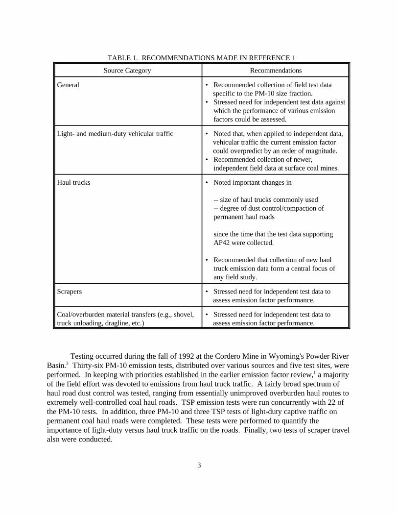
TABLE 1. RECOMMENDATIONS MADE IN REFERENCE 1
Source Category Recommendations
General • Recommended collection of field test data specific to the PM-10 size fraction.• Stressed need for independent test data against
which the performance of various emissionfactors could be assessed.
Light- and medium-duty vehicular traffic • Noted that, when applied to independent data, vehicular traffic the current emission factor could overpredict by an order of magnitude.• Recommended collection of newer,
independent field data at surface coal mines.
Haul trucks • Noted important changes in
-- size of haul trucks commonly used-- degree of dust control/compaction ofpermanent haul roads
since the time that the test data supportingAP42 were collected.
• Recommended that collection of new haultruck emission data form a central focus ofany field study.
Scrapers • Stressed need for independent test data to assess emission factor performance.
Coal/overburden material transfers (e.g., shovel,truck unloading, dragline, etc.)
• Stressed need for independent test data to assess emission factor performance.
Testing occurred during the fall of 1992 at the Cordero Mine in Wyoming's Powder RiverBasin.3 Thirty-six PM-10 emission tests, distributed over various sources and five test sites, wereperformed. In keeping with priorities established in the earlier emission factor review,1 a majorityof the field effort was devoted to emissions from haul truck traffic. A fairly broad spectrum ofhaul road dust control was tested, ranging from essentially unimproved overburden haul routes toextremely well-controlled coal haul roads. TSP emission tests were run concurrently with 22 ofthe PM-10 tests. In addition, three PM-10 and three TSP tests of light-duty captive traffic onpermanent coal haul roads were completed. These tests were performed to quantify theimportance of light-duty versus haul truck traffic on the roads. Finally, two tests of scraper travelalso were conducted.
4
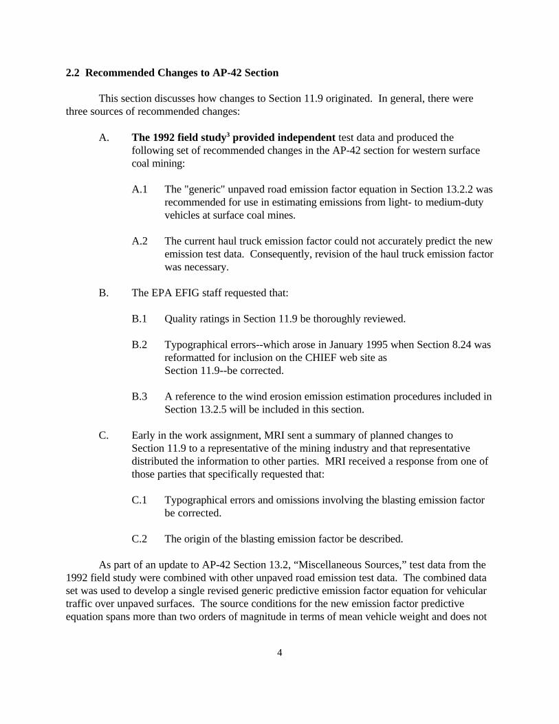
2.2 Recommended Changes to AP-42 Section
This section discusses how changes to Section 11.9 originated. In general, there werethree sources of recommended changes:
A. The 1992 field study3 provided independent test data and produced thefollowing set of recommended changes in the AP-42 section for western surfacecoal mining:
A.1 The "generic" unpaved road emission factor equation in Section 13.2.2 wasrecommended for use in estimating emissions from light- to medium-dutyvehicles at surface coal mines.
A.2 The current haul truck emission factor could not accurately predict the newemission test data. Consequently, revision of the haul truck emission factorwas necessary.
B. The EPA EFIG staff requested that:
B.1 Quality ratings in Section 11.9 be thoroughly reviewed.
B.2 Typographical errors--which arose in January 1995 when Section 8.24 wasreformatted for inclusion on the CHIEF web site asSection 11.9--be corrected.
B.3 A reference to the wind erosion emission estimation procedures included inSection 13.2.5 will be included in this section.
C. Early in the work assignment, MRI sent a summary of planned changes toSection 11.9 to a representative of the mining industry and that representativedistributed the information to other parties. MRI received a response from one ofthose parties that specifically requested that:
C.1 Typographical errors and omissions involving the blasting emission factorbe corrected.
C.2 The origin of the blasting emission factor be described.
As part of an update to AP-42 Section 13.2, “Miscellaneous Sources,” test data from the1992 field study were combined with other unpaved road emission test data. The combined dataset was used to develop a single revised generic predictive emission factor equation for vehiculartraffic over unpaved surfaces. The source conditions for the new emission factor predictiveequation spans more than two orders of magnitude in terms of mean vehicle weight and does not

5
Sizerange Run
Measuredemissionfactors
(lb/VMT)
AP-42 Section13.2.2
estimates(Ib/VMT)
Predictedto
observedratio
PM-10 BB-44 0.25 0.24 0.976
PM-10 BB-45 0.078 0.26 3.35
PM-10 BB-48 0.12 0.26 2.19
Geometric mean 0.13 0.25 1.91
TSP BB-44 1.3 0.54 0.426
TSP BB-45 0.60 0.58 0.960
TSP BB-48 0.49 0.58 1.19
Geometric mean 0.72 0.57 0.786
exhibit any systematic bias for the individual subsets (e.g., haul trucks at mines, light-duty vehicleson publicly accessible roads, scrapers in travel mode, etc.) that constitute the expanded data base. The background document (Ref 7) for the revised Section 13.2.2, “Unpaved Roads,” describesthe development and validation of the unpaved road emission factor equation.
Also as part of the 1997 update to AP-42, EPA requested additional information onemission tests underlying the current version of Section 11.9. A series of appendices have beenprepared to make this information available through the EPA’s Technology Transfer Network(TTN).
2.3 Revisions to AP-42 Section
The previous section discussed the origin of recommended changes to AP-42Section 11.9. This section describes how each change was made.
Change A.1-Substitution of the generic unpaved road emission factor for the formerlight-/medium-duty vehicle frame emission factor. The 1992 field study provided newindependent test data against which the recommended factor could be evaluated. Although inmany cases, the AP-42 Section 8.24 model had been found to produce very accurate estimates thesame model had been found to be capable of providing very unacceptable estimates in other cases. This variation is believed to have been the result of the model's dependence on the fourth powerof moisture content.
Table 2 compares the 1992 test results to estimates obtained from the Section 13.2.2"generic" model that is recommended in place of the Section 8.24 model.
6
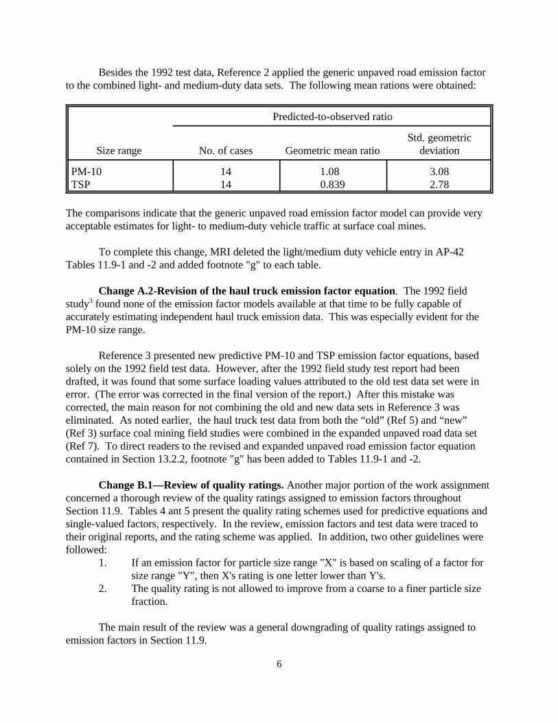
Besides the 1992 test data, Reference 2 applied the generic unpaved road emission factorto the combined light- and medium-duty data sets. The following mean rations were obtained:
Size range
Predicted-to-observed ratio
No. of cases Geometric mean ratioStd. geometric
deviation
PM-10TSP
1414
1.08 0.839
3.082.78
The comparisons indicate that the generic unpaved road emission factor model can provide veryacceptable estimates for light- to medium-duty vehicle traffic at surface coal mines.
To complete this change, MRI deleted the light/medium duty vehicle entry in AP-42Tables 11.9-1 and -2 and added footnote "g" to each table.
Change A.2-Revision of the haul truck emission factor equation. The 1992 fieldstudy3 found none of the emission factor models available at that time to be fully capable ofaccurately estimating independent haul truck emission data. This was especially evident for thePM-10 size range.
Reference 3 presented new predictive PM-10 and TSP emission factor equations, basedsolely on the 1992 field test data. However, after the 1992 field study test report had beendrafted, it was found that some surface loading values attributed to the old test data set were inerror. (The error was corrected in the final version of the report.) After this mistake wascorrected, the main reason for not combining the old and new data sets in Reference 3 waseliminated. As noted earlier, the haul truck test data from both the “old” (Ref 5) and “new”(Ref 3) surface coal mining field studies were combined in the expanded unpaved road data set (Ref 7). To direct readers to the revised and expanded unpaved road emission factor equationcontained in Section 13.2.2, footnote "g" has been added to Tables 11.9-1 and -2.
Change B.1—Review of quality ratings. Another major portion of the work assignmentconcerned a thorough review of the quality ratings assigned to emission factors throughoutSection 11.9. Tables 4 ant 5 present the quality rating schemes used for predictive equations andsingle-valued factors, respectively. In the review, emission factors and test data were traced totheir original reports, and the rating scheme was applied. In addition, two other guidelines werefollowed:
1. If an emission factor for particle size range "X" is based on scaling of a factor forsize range "Y", then X's rating is one letter lower than Y's.
2. The quality rating is not allowed to improve from a coarse to a finer particle sizefraction.
The main result of the review was a general downgrading of quality ratings assigned toemission factors in Section 11.9.

7
TABLE 4. QUALITY RATING SCHEME FOR SINGLE-VALUED EMISSION FACTORS
CodeNo. of
test sitesNo. of tests
per siteTotal No.of tests
Test datavariabilitya
Adjustmentfor EFratingb
1 $3 $3 - <F2 0
2 $3 $3 - >F2 -1
3 2 $2 $5 <F2 -1
4 2 $2 $5 >F2 -2
5 - - $3 < F2 -2
6 - - $3 >F2 -3
7 1 2 2 <F2 -3
8 1 2 2 >F2 -4
9 1 1 1 - -4aData spread in relation to central value. F2 denotes factor of two.bDifference between emission factor rating and test data rating.
TABLE 5. QUALITY RATING SCHEME FOR EMISSION FACTOR EQUATIONS
CodeNo. of
test sitesNo. of tests
per siteTotal No.of testsa
Adjustment for EFratingb
1 $3 $3 $(9 + 3P) 0
2 $2 $3 $3P -1
3 $1 -- <3P -2aP denotes number of correction parameters in emission factor equation.bDifference between emission factor rating and test data rating.
Change B.2—Correction of typographical errors in Section 11.9. A variety of errorshad been noted and were corrected.
Change B.3—Use of the generic wind erosion procedure. Much of the data basesupporting AP-42 Section 13.2.5 ("Industrial Wind Erosion") pertains to coal surfaces. A newfootnote has been added to AP-42 Tables 11.9-1 and -2 to direct readers to consider the use ofSection 13.2.5 to estimate emissions from wind erosion.

8
Change C.1—Correction of typographical error and omissions in the blastingemission factor. As noted at the beginning of Section 2.1, AP-42 Section 8.24 was revisedduring the 1980s to change the predictive emission factor equation for blasting. (This revision isdiscussed in more detail below.) However, the metric and English versions of the equation didnot correspond to one another, and no units were specified for the input variable. These errorswere corrected.
Change C.2—Origin of the revised blasting emission factor predictive equation. Asnoted above, the blasting emission factor in Tables 8.24-1 and -2 was revised during the 1980s. When Section 8.24 was first drafted in 1983, it included TSP and PM-15 predictive emissionfactor equations for blasting, of the general form
e = k (A)a / (D)b (M)d (2)
where:e = emission factor, expressed in mass of emissions per blastA = area blasted (area)D = hole depth (length)M = material moisture content (fraction)
and k, a, b, and c regression-based values, all greater than zero. In particular, the exponent formoisture was approximately 2. This functional form was first developed in Reference 1. Inaddition, a PM-2.5 emission factor was developed and was presented as 0.03 of the TSP emissionfactor. The PM-2.5 to TSP ratio was based upon the geometric mean of the 19 coal andoverburden blasting tests that were conducted.
In September 1985, EPA included the unchanged Section 8.24 blasting equation inSection 8.18.2 ("Crushed Stone Processing"). By 1986, crushed stone industry representativeshad raised concerns and questioned the appropriateness of the moisture term for stone. Theynoted that moisture values in the coal mining data set were easily an order of magnitude or greaterthan values for stone.
In 1986, EPA asked Midwest Research Institute under a level-of-effort contract to reviewavailable blasting emission test data. In June of 1986, MRI sent a letter to OAQPS that presentedthe results from that review. (A copy of that letter is contained in Appendix E.) This letterpresented the following emission factor for use in the crushed stone industry, based on areexamination of the original (surface coal mining) data set:
e = 0.00050 (A)1.5 (3)
where:
e = TSP emission factor (lb/blast)A = area blasted (m2)
9
Later, MRI submitted draft interim guidance materials on estimating emissions fromblasting at both surface coal mining and stone operations. (A copy of that material is alsopresented in Appendix E). Because equation (3) was developed from coal mining test data, thatequation was recommended for use in estimating emissions at surface coal mines. In addition, aPM-10 to TSP ratio of 0.52 was suggested, based on the analogy with particle size data collectedduring emission tests of material handling operations. In the revisions to the section, the ratio ofPM-2.5 to TSP of 0.03 was dropped from the blasting emission factor table.
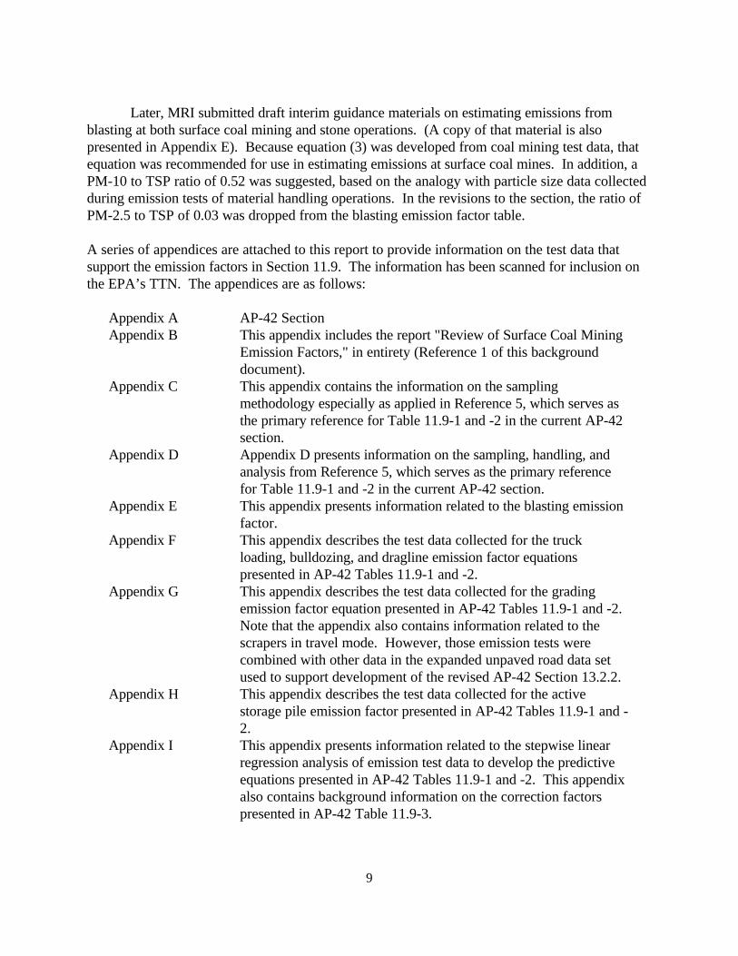
A series of appendices are attached to this report to provide information on the test data thatsupport the emission factors in Section 11.9. The information has been scanned for inclusion onthe EPA’s TTN. The appendices are as follows:
Appendix A AP-42 SectionAppendix B This appendix includes the report "Review of Surface Coal Mining
Emission Factors," in entirety (Reference 1 of this backgrounddocument).
Appendix C This appendix contains the information on the samplingmethodology especially as applied in Reference 5, which serves asthe primary reference for Table 11.9-1 and -2 in the current AP-42section.
Appendix D Appendix D presents information on the sampling, handling, andanalysis from Reference 5, which serves as the primary referencefor Table 11.9-1 and -2 in the current AP-42 section.
Appendix E This appendix presents information related to the blasting emissionfactor.
Appendix F This appendix describes the test data collected for the truckloading, bulldozing, and dragline emission factor equationspresented in AP-42 Tables 11.9-1 and -2.
Appendix G This appendix describes the test data collected for the gradingemission factor equation presented in AP-42 Tables 11.9-1 and -2. Note that the appendix also contains information related to thescrapers in travel mode. However, those emission tests werecombined with other data in the expanded unpaved road data setused to support development of the revised AP-42 Section 13.2.2.
Appendix H This appendix describes the test data collected for the activestorage pile emission factor presented in AP-42 Tables 11.9-1 and -2.
Appendix I This appendix presents information related to the stepwise linearregression analysis of emission test data to develop the predictiveequations presented in AP-42 Tables 11.9-1 and -2. This appendixalso contains background information on the correction factorspresented in AP-42 Table 11.9-3.
10
Section 3References
1. G. E. Muleski, Review of Surface Coal Mining Emission Factors, EPA-454/R-95-007,U. S. Environmental Protection Agency, Research Triangle Park, NC, July 1991.
2. G. E. Muleski and C. Cowherd, Jr., Surface Cal Mine Study Plan, EPA-454/R-95-009,U. S. Environmental Protection Agency, Research Triangle Park, NC, March 1992.
3. G. E. Muleski and C. Cowherd, Jr., Surface Coal Mine Emission Factor Field Study,EPA-454/R-95-010, U. S. Environmental Protection Agency, Research Triangle Park,NC, January 1994.
4. C. Cowherd, Jr., B. Petermann, and P. Englehart, Fugitive Dust Emission Factor Updatefor AP-42. EPA Contract 68-02-3177, Work Assignment 25, September 1983.
5. Improved Emission Factors for Fugitive Dust From Western Surface Coal Mines,EPA-600/7-84-048, U. S. Environmental Protection Agency, Volumes I and II, March1984.
6. Shearer, D.L., R.A. Dougherty, and C.C. Easterbrook, Coal Mining Emission FactorDevelopment and Modeling Study, TRC Environmental Consultants, July 1981.
7. Emission Factor Documentation for AP-42 Section 13.2.2, Unpaved Roads (Draft),Midwest Research Institute, EPA Contract 68-D2-0159, Work Assignment 4-02,September 1997.

Appendices
i
TABLE OF CONTENTSPage
Appendix A -- Revised AP-42 Section 11.9 . . . . . . . . . . . . . . . . . . . . . . . . . . . . . . . . . . . . . . A-1
Appendix B -- "Review of Surface Coal Mining Emission Factors" . . . . . . . . . . . . . . . . . . . . B-1
Appendix C -- Sampling Methodology . . . . . . . . . . . . . . . . . . . . . . . . . . . . . . . . . . . . . . . . . . C-1C.1 -- Section 4.2 of Report: "Fugitive Dust Emission Factor
Update for AP-42" . . . . . . . . . . . . . . . . . . . . . . . . . . . . . . . . . . . . . . . . . . . . . C-3C.2 -- Section 3 of Report: "Improved Emission Factors for Fugitive
Dust from Western Surface Coal Mining Sources--Volume 1 - Sampling Methodology and Test Results" . . . . . . . . . . . . . . . . . . . . . . . . . . C-8
Appendix D -- Sample Handling and Analysis . . . . . . . . . . . . . . . . . . . . . . . . . . . . . . . . . . . . D-1D.1 -- Section 4 of Report: "Improved Emission Factors for Fugitive
Dust from Western Surface Coal Mining Sources--Volume 1 - Sampling Methodology and Test Results" . . . . . . . . . . . . . . . . . . . . . . . . . . D-3
Appendix E -- Materials Related to Blasting Emission Factor . . . . . . . . . . . . . . . . . . . . . . . . . E-1E.1 -- Section 5.5 and 8.5 of "Fugitive Dust Emission Factor Update
for AP-42 . . . . . . . . . . . . . . . . . . . . . . . . . . . . . . . . . . . . . . . . . . . . . . . . . . . . E-3E.2 -- Memorandum from Chatten Cowherd, MRI, to James Southerland,
EPA, June 1986 . . . . . . . . . . . . . . . . . . . . . . . . . . . . . . . . . . . . . . . . . . . . . . E-26E.3 -- Memorandum from Greg Muleski, MRI, to Frank Noonan,
EPA, April 1987 . . . . . . . . . . . . . . . . . . . . . . . . . . . . . . . . . . . . . . . . . . . . . . E-30E.4 -- Section 9 of “Improved Emission Factors For Fugitive Dust
From Western Surface Coal Mining Sources--Volume I -Sampling Methodology and Test Results” . . . . . . . . . . . . . . . . . . . . . . . . . . E-34
Appendix F -- Materials Related to Truck Loading, Bulldozing, and Dragline Emission Factors . . . . . . . . . . . . . . . . . . . . . . . . . . . . . . . . . . . . . . . F-1
F.1 -- Sections 5.5 and 8.5 of EPA report "Fugitive Dust Emission Factor Update for AP-42" . . . . . . . . . . . . . . . . . . . . . . . . . . . . . . . . . . . . . . . . . . . . . F-3
F.2 -- Section 8 of EPA report "Improved Emission Factors for Fugitive Dust from Western Surface Coal Mining Sources--Volume I - Sampling Methodology and Test Results . . . . . . . . . . . . . . . . . . . . . . . . . . F-25
Appendix G -- Materials Related to Scraper and Grading Emission Factors . . . . . . . . . . . . . . G-1G.1 -- Sections 5.5 and 8.5 of EPA report "Fugitive Dust Emission Factor
Update for AP-42" . . . . . . . . . . . . . . . . . . . . . . . . . . . . . . . . . . . . . . . . . . . . . G-3
TABLE OF CONTENTS (CONTINUED)Page
ii
G.2 -- Section 7 of EPA report "Improved Emission Factors for Fugitive Dust From Western Surface Coal Mining Sources--Volume I - Sampling Methodology and Test Results" . . . . . . . . . . . . . . . . . . . . . . . . . G-26
Appendix H -- Materials Related to Active Storage Pile Emission Factor . . . . . . . . . . . . . . . . H-1H.1 -- Sections 5.5 and 8.5 of EPA report "Fugitive Dust Emission Factor
Update for AP-42" . . . . . . . . . . . . . . . . . . . . . . . . . . . . . . . . . . . . . . . . . . . . . H-3H.2 -- Section 10 of EPA report "Improved Emission Factors For Fugitive
Dust From Western Surface Coal Mining Sources --Volume I - Sampling Methodology and Test Results" . . . . . . . . . . . . . . . . . . . . . . . . . H-22
Appendix I -- Development of Correction Factors and Emission Factor Equations . . . . . . . . . I-1I.1 -- Sections 5 and 13, and Appendices A and B of the EPA report “Improved
Emission Factors For Fugitive Dust From Western Surface Coal Mining Sources - Volume I and 11.” . . . . . . . . . . . . . . . . . . . . . . . . . . . . . . . . . . . . . I-3

Appendix ARevised AP-42 Section 11.9
October 1997
This appendix contains revisions to AP-42 Section 11.9 "Western Surface Coal Mining." The
purpose of the changes was to improve emission factors contained in AP-42, "Compilation of Air Pollutant
Emission Factors." The revised AP-42 Section was removed from this file and is located in a seperate file.

Appendix B“Review of Surface Coal Mining Emission Factors”
This appendix contains the interim EPA report “Review of Surface Coal Mining Emission
Factors,” in entirety. The report provides a review of held-measurement-based emission factors for surface
coal mines and describes held testing needs to address gaps in the data base.
United States Office of Air Quality EPA-454/R-95-007Environmental Protection Planning and Standards July 1991Agency Research Triangle Park, NC 27711Air
REVIEW OF
SURFACE COAL MINING
EMISSION FACTORS

EPA-45/R-95-007
REVIEW OF
SURFACE COAL MINING
EMISSION FACTORS
Emission Factor And Inventory GroupEmissions, Monitoring, And Analysis Division
U. S. Environmental Protection AgencyResearch Triangle Park, NC 27711
July 1991

This report has been reviewed by the Office of Air Quality Planning And Standards, U. S.Environmental Protection Agency, and has been approved for publication. Any mention of the trade namesor commercial products is not intended to constitute endorsement or recommendation for use.
EPA-45/R-95-007
B-5
PREFACE
This interim report was prepared by Midwest Research Institute under U.S. EnvironmentalProtection Agency (EPA) Contract No. 68-DO-0137, Work Assignment No. 10. The principal author ofthis report is Dr. Greg Muleski; he was assisted by Mr. Robert Dobson and Ms. Karen Connery.Mr. Dennis Shipman of the Office of Air Quality Planning and Standards serves as the EPA's technicalmonitor of the work assignment.
Approved:
Charles F. Holt, Ph.D., DirectorEngineering and Environmental Technology Department
July 11, 1991

B-6

B-7
CONTENTS
1. Introduction . . . . . . . . . . . . . . . . . . . . . . . . . . . . . . . . . . . . . . . . . . . . . . . . . . . . . . . . B-82. Overview of the Surface Coal Mining Industry . . . . . . . . . . . . . . . . . . . . . . . . . . . . . . B-103. Overview of Emission Sources and Measurements at Surface Coal Mines . . . . . . . . . . B-13
Important Emission Sources . . . . . . . . . . . . . . . . . . . . . . . . . . . . . . . . . . . . . . . . B-13Field Measurements at Surface Coal Mines . . . . . . . . . . . . . . . . . . . . . . . . . . . . . B-14
4. Emission Factors For Use at Surface Coal Mines . . . . . . . . . . . . . . . . . . . . . . . . . . . . . B-18AP-42 Emission Factors and Predictive Equations . . . . . . . . . . . . . . . . . . . . . . . . B-18Evaluation of Alternative Emission Factors . . . . . . . . . . . . . . . . . . . . . . . . . . . . . B-19
5. Summary and Recommendations . . . . . . . . . . . . . . . . . . . . . . . . . . . . . . . . . . . . . . . . . B-276. References . . . . . . . . . . . . . . . . . . . . . . . . . . . . . . . . . . . . . . . . . . . . . . . . . . . . . . . . . B-49
B-8
SECTION 1
INTRODUCTION
As part of the Clean Air Act Amendments of 1990, the U.S. Environmental Protection Agency has
the need to review and revise emission factors for criteria pollutants. Specifically, Section 234 of Title I
requires field testing for emission factors for surface coal mines. This interim report provides a review of
currently available, field-measurement-based emission factors for surface coal mines (SCMs) and describes
field testing needs to address gaps in the data base.
A principal purpose of the review is to provide a common basis for discussion at a workshop to be
held in Kansas City, Missouri, during August 1991. This report has been sent to interested parties who
have been invited to participate at the workshop. These parties include coal and mining industry groups,
environmental organizations, and state and federal agencies for mining activities and environmental
protection.
Throughout the report, the review focuses on the strengths and weaknesses of the available data,
thus identifying major gaps within the data base.
The remainder of this report is structured as follows. Section 2 presents a brief overview of the
surface coal mining industry. Section 3 describes the types of emission sources found at SCMs,
emphasizing operating characteristics that are potentially different between various parts of the country. In
Section 4, the methods available to estimate emissions from SCM sources are discussed and major gaps
within the data base are identified. Section 5 summarizes the results of the review and presents a series of
recommendations. Section 6 lists the references cited in the report.
Emission factors relate the amount of mass emitted per unit activity of the source. For example, a
common unit for travel related emissions is “lb/vmt,” or pounds emitted per vehicle mile traveled. Thus,
the “source extent” on a road is measured in terms of the total miles traveled by vehicles over the road.
Similarly, if a material handling emission factor is expressed in terms of pounds emitted per ton (or, cubic
yard), then the source extent is measured in terms of the tons or cubic yards of material transferred.
The following discussion uses English—such as pounds and miles—rather than metric (Sl)
units—such as kilograms and kilometers. This approach has been taken because it is believed that
individuals taking part in the Kansas City workshop will be more familiar with common English units.

B-9
The principal pollutant of interest in this report is “particulate matter” (PM), with special emphasis
placed on “PM-10" or (particulate matter no greater than 10 Fma (microns in aerodynamic diameters).
PM-10 is the basis for the current National Ambient Air Quality Standards (NAAQSs) for particulate
matter as well as the EPA's Prevention of Significant Deterioration (PSD) increments.
PM-10 thus represents the size range of particulate matter that is of the greatest regulatory interest.
Nevertheless, formal establishment of PM-10 as the standard basis is relatively recent, and virtually all
surface coal mine field measurements reflect a particulate size other than PM-10. Other size ranges
employed in this report are:
TSP Total Suspended Particulate, as measured by the standard high-volume (hi-vol) air
sampler. TSP was the basis for the previous NAAQSs and PSD increments. TSP is a
relatively coarse size fraction. While the capture characteristics of the hi-vol sampler are
dependent upon approach wind velocity, the effective D50 (i.e., 50 percent of the particles
are captured and 50 percent are not) varies roughly from 25 to 50 Fma.
SP Suspended Particulate, which is used as a surrogate for TSP. Defined as PM no greater
than 30 Fma. Also denoted as “PM-30.”
IP Inhalable Particulate, defined as PM no greater than 15 Fma. Throughout the late 1970s
and the early 1980s, it was clear that EPA intended to revise the NAAQSs to reflect a size
range finer than TSP. What was not clear was the size fraction that would be eventually
used, with values between 7 and 15 Fma frequently mentioned. Thus, many field studies at
SCMs were conducted using IP measurements because it was believed that would be the
basis for the new NAAQS. IP may also be represented by “PM-15.”
FP Fine Particulate, defined as PM no greater than 2.5 Fma. Also denoted as “PM-2.5.”
It is again emphasized that this is an interim report whose purpose is to provide a common basis
for further discussion at the Kansas City workshop. It is probable that several issues in addition to those
presented here will be raised at the workshop. This report, then, is an initial focus point for constructive
discussions and, in that sense, represents very much a “work in progress.”

B-10
SECTION 2
OVERVIEW OF THE SURFACE COAL MINING INDUSTRY
Coal is mined in 26 states. The leading coal producers are Kentucky, Wyoming, West Virginia,
Pennsylvania, Illinois, Texas, Virginia, and Ohio; these states account for approximately 75% of U.S. coal
production.1
United States coal reserves total approximately 490 billion tons. Of that total, 330 billion tons are
estimated to be minable by underground methods and 160 billion tons by surface methods. Since the early
1970s surface mines have accounted for more than half of the total coal produced. In 1985 coal was
produced by both underground and surface mining in 15 of the 26 coal-producing states, with the remaining
11 having surface mines only.
For discussion purposes in this report, the U.S. coal mining industry has been divided into three
major regions:
• Appalachian Region
- Northern Appalachia
- Central Appalachia
- Southern Appalachia
• Midwest Region
• West Region
- Powder River
- Rocky Mountain
(The small amount of coal mining in Alaska is not considered in this report.) Each region and subregion is
briefly described in the following paragraphs.2
Northern Appalachia includes the states of Maryland, Pennsylvania, Ohio, and northern West
Virginia. Coal production is largely high to medium sulfur bituminous coal. Eastern Pennsylvania is home
to the only working anthracite mines in the United States. Bituminous coal production in the Northern
Appalachian Region totaled 155.5 million tons in 1985 of which 62.2 million tons were surface mined and
93.4 were mined using underground methods (see Figure 1). Northern Appalachia is characterized by a
small number of underground mines and a large number of very small surface operations.

B-11
Central Appalachia includes areas in Southern West Virginia, Virginia, the eastern half of
Kentucky, and Northern Tennessee. The coal reserve base is approximately 52 billion tons of bituminous
coal, of which 7.9 billion tons are minable by surface methods and 44.1 billion tons are recoverable by
underground methods. Production in 1985 was 232.4 million tons of which 72.1 million tons were surface
mined (see Figure 2).
Central Appalachia is characterized by a large number of “mom and pop” surface and underground
mines. The mines are termed in this way due to the small, informal, family nature of most of the
operations.
Southern Appalachia includes the mining areas of Alabama and southern Tennessee. The reserve
base totals 4.9 billion tons of bituminous coal split equally between surface and underground mining
methods. A 1-billion ton reserve of lignite is not presently mined. Production of bituminous coal in
Southern Appalachia totaled 30.1 million tons in 1985 of which 13.9 million tons were surface mined.
Southern Appalachia is characterized by a few producers with large capacity underground mines, and
medium to small surface mines (see Figure 3).
The Midwest Region includes regions of Illinois, Indiana, and western Kentucky and is also known
as the Illinois Coal Basin. The entire 110 billion ton reserve base is bituminous. Of this total, 21 billion
tons are surface minable. Coal production in the Midwest totaled 131.4 million tons in 1985 (74.1 million
tons surface mined).
The Midwest Region is characterized by large corporate mines. This is particularly true of
underground mines. As shown in Figure 4, Midwest surface mines are quite uniformly distributed over a
very broad range of annual production values.
Western coal mining is divided into two areas, the Rocky Mountain Region and the Powder River
Basin. The Powder River Basin includes Montana and Wyoming. The reserve base ranges from lignite to
reasonably high quality bituminous. The total reserve base is 189.4 billion tons, of which 168 billion tons
is classified as subbituminous, 16 billion tons as lignite, and 6 billion tons as bituminous. Production in the
Powder River Basin totaled 174 million tons in 1985, virtually all of which was surface mined (Figure 5).
The Powder River Basin is characterized by very large surface mines, with the largest mines in the United
States in this region.
The Rocky Mountain Region includes the states of Colorado, Utah, New Mexico, and Arizona.
This region has reserves in four different classifications: anthracite, bituminous, subbituminous, and lignite.
Recoverable reserves total 18.5 billion tons, of which 8 billion tons are considered minable by surface
methods.
B-12
Coal production in the Rocky Mountain Region totaled 61.9 million tons in 1985 of which
42 million tons were surface mined. The total consisted of bituminous and subbituminous coal. Large
surface operations and large underground operations characterize the region (see Figure 6).
Tables 1 and 2 provide summary information for the 1985 United States coal production in the
Appalachian/Midwest and West regions, respectively.
In summary, the number of mines increases and the average size decreases as one considers U.S.
surface coal mines from east to west. The Appalachian Region has many small surface operations while
the relatively few western mines are almost all very large. The Midwest Region represents the transition
between the two extremes, with surface mines in all size ranges relatively common.
Approximately 50% of the coal surface mined in the United States is from eastern regions, where
mines tend to be relatively small. As will be seen in the next section, emissions from eastern SCMs have
not been considered to any great extent. Consequently, potential differences in PM emissions due not only
to the different size of mines, but also different climate factors in the east, have not been fully
characterized.

B-13
SECTION 3
OVERVIEW OF EMISSION SOURCES AND MEASUREMENTS AT SURFACE COAL MINES
Throughout the surface mining process—from initial removal of topsoil until final
reclamation—particulate matter (PM) may be emitted from a variety of operations. This Section (a)
discusses major PM emission sources at surface coal mines and (b) provides a short history of field
measurement of those emission sources.
IMPORTANT EMISSION SOURCES
Table 3 summarizes particulate matter emission sources typically found at surface coal mines; the
operations listed in the Table are largely sequential. All sources may be present simultaneously throughout
different areas at any one mine.
Clearly, PM sources vary in importance not only from one mine to another—depending on, say,
strip ratios or the type of equipment used (power shovel, dragline, bucket wheel excavator [BWE])—but
also from one time to another at the same mine—for example, when haul distances and hence haulage-
related emissions are the greatest.
Several prior studies have examined, in general terms, the relative importance of different emission
sources at SCMs. Inventories of hypothetical examples as well as of actual mines indicate that typically
over half (roughly 60% to 90%) of the total suspended particulate (TSP) emission rate is due to the
following four traffic-related sources:
• scraper travel
• coal haul trucks
• overburden haul trucks
• general (light and medium duty) traffic
Not all of the four sources are necessarily important at every mine. For example, overburden haul
trucks are not used at a dragline mine; in that case, overburden removal by dragline becomes far more
important. Also, general traffic might not be important at, say, small mines with deep coal seams.
In very general terms, the four traffic-related sources listed above plus overburden removal by
dragline should account for roughly 70% of total TSP emissions at most large surface mines.3

B-14
FIELD MEASUREMENTS AT SURFACE COAL MINES
Since 1973, production in U.S. western mines has more than tripled.1,2 The expansion is in large
part the result of events during the early 1970s: the original Clean Air Act resulted in high demand for low-
sulfur western coals, and the 1973 oil embargo stressed the importance of energy independence and spurred
mining activities. Thus, the development of large western SCMs was accompanied by a more widespread
interest in protecting the environment.
It is not surprising, then, that essentially all of the available field measurement data base (a) dates
from the late 1970s and early 1980s and (b) primarily reflects western SCMs. Consequently, two
limitations of available data become immediately apparent:
1. Eastern surface coal mines may not be well characterized in terms of emission characteristics.
Recall that these mines tend to be substantially smaller in terms of production and disturbed
area. In addition, there has long been a suspicion that open dust emission levels differ
substantially between the eastern and western United States. This point is discussed further in
the next section.
2. Throughout the country, available field measurements generally do not reference the particle
size range of current regulatory interest, because of the relatively recent emergence of PM-10
as the basis for the PM NAAQSs. Furthermore, some field measurements have been found to
be unreliable in terms of particle size characterization. This, too, is discussed in Section 4.0.
Table 4 summarizes major field measurement studies undertaken to determine emission factors
generally applicable for SCMs.5-8 Note that only two of the test programs considered mines east of the
Mississippi River. The PEDCo/MRI study forms the principal basis for EPA's recommended emission
factors for western surface coal. These factors are included in Section 8.24 of the EPA publication
“Compilation of Air Pollutant Emission Factors,” commonly referred to as “AP-42.”9
Throughout the next section, it is assumed that the reader is familiar with common open dust
source measurement techniques such as “upwind/ downwind” and “exposure profiling.” Detailed
descriptions of open source measurement methodologies are available elsewhere.10
The EDS study was conducted to develop PM emission factors for primary surface mining
activities. Two mines in the Powder River Basin were considered, with tests conducted between fall 1978
and summer 1979. Emission factors are presented for the following sources:
trucks hauling coal or overburden (with and without watering as a control measure)
coal dumping
train loading

B-15
overburden replacement
topsoil removal by scrapers
wind erosion of stripped overburden and reclaimed land
With the exception of haul trucks, emissions were characterized using an upwind/downwind
approach; haul truck tests employed exposure profiling. Results are summarized in Table 5. TSP was the
particle size range of interest.
This industry-sponsored program paid particular attention to particle deposition and its
implications for dispersion modeling. Emission factors are presented not only for at-source conditions, and
“apparent” factors are given for distances of 500 and 1,000 m. At-source emission factors have largely
been incorporated into AP-42 Section 8.24.
The PEDCo/MRI study was conducted with the express goal of developing emission factor
equations for western SCM operations. TSP, IP, SP, and FP were the size ranges of interest. Three
mines—in the Fort Union, the Powder River, and the San Juan Fields—were considered over the summer
and fall of 1979 and the summer of 1980.
A combination of the exposure profiling, upwind/downwind, and portable wind tunnel sampling
methodologies were employed to characterize emissions from the sources listed in Table 6, which
summarizes the upwind/downwind and exposure profiling tests emissions testing conducted. Wind tunnel
measurements and wind erosion emission factors are described later.
As noted earlier, this study provides most of the experimental basis for AP-42 Section 8.24.
The Skelly and Loy study, conducted as one part of an EPA contract, is the only field program in
Table 4 devoted entirely to eastern surface coal mining. Upwind/downwind field measurements were
collected over a short, 10-day period to determine TSP emission factors for
haul trucks
drilling/overburden removal/coal loading (considered as one source)
regrading of land where coal had been removed
See Table 7.
The scope and extent of this “screening type” study are much more limited than those for the other
programs listed in Table 4. In addition, the authors noted that wind speeds and haul truck travel speeds
were substantially higher than in the western studies. Consequently, it is very difficult to interpret the
Skelly & Loy emission factors that are roughly an order of magnitude greater than corresponding western
results. At the very least, however, this study indicates a need for further characterization of PM emissions
at eastern SCMs.
B-16
The scope of the PEDCo/BuMines study was much more focused than the other studies in Table 4.
While the other programs considered several emission sources, this program was undertaken to determine
the efficiency and cost-effectiveness of dust controls applied to SCM haul roads. Tests were conducted at
three mines—including one east of the Mississippi—during the summer and fall of 1982. Types of
controls considered included: salts, surfactants, adhesives, bitumens, films, and plain water. Table 8
summarizes results of this test program.
Three points should be noted about this study. First, the report states that, because of the emphasis
on control efficiencies, there was no attempt made to develop general emission factors for unpaved haul
roads.
Second, exposure profiling measurements were made using stacked filtration units (SFUs). The
SFUs were designed to produce data for the SP and FP size fractions. However, an independent contractor
has found that the SFU collection media were selected on the basis of pore size and collection efficiency
was not verified through calibration. A 1985 collaborative study of five different exposure profiling
systems found that, as samples are collected, SFUs become more efficient. As a consequence,
concentration and emission factors are systematically underestimated.12,13 Overall, the independent
evaluation concluded that SFUs could not be recommended for open dust emission characterization. As a
result, this independent emissions data base is of little value in judging the “predictive accuracy” of haul
road emissions factors.
Finally, much of the control efficiency data in the PEDCo/BuMines exhibit anomalous behavior,
such as showing increased efficiency over time. It is believed that much of this is due to the fact that
control efficiencies were not referenced to dry, uncontrolled emissions. A 1987 update to Section 11.2 of
AP-42 demonstrated the regulatory importance of referencing unpaved road efficiency to worst-case
conditions.13
Besides studies specifically directed toward surface coal mines, other field programs have
produced emission factors that are applicable to a wide range of sources at SCMs. Field tests have been
conducted on public roads as well as in various industries, including coal-fired power plants, iron and steel
plants, stone quarrying, mining, and smelting operations. The results of these tests have been incorporated
into “generic” emission factor models.
Section 11.2 of AP-42 presents generic open dust emission factors which can be applied to the
following SCM sources
• scraper travel
• material handling activities for topsoil, overburden, and coal

B-17
• haul roads for both overburden and coal
• loading and unloading of trucks
• loadout for transit
• general traffic
Note that generic emission factors are available for the four or five most important emission sources
identified earlier.
Finally, as part of a recently completed study for the State of Arizona, MRI conducted a critical
review of unpaved road emission estimations.14 The review encompassed the PEDCo/MRI data.6 Pertinent
results from this study are discussed in the next section.

B-18
SECTION 4
EMISSION FACTORS FOR USE AT SURFACE COAL MINES
The preceding Section described common PM emission sources and past field measurement efforts
at SCMs. This Section first describes EPA guidance on emission estimation for SCMs and then presents a
critical review of available emission factors.
AP-42 EMISSION FACTORS AND PREDICTIVE EQUATIONS
EPA publication AP-42, “Compilation of Air Pollutant Emission Factors,” represents official
agency guidance on the emission factors to be used for a wide variety of process, open, and mobile
emission sources. Section 8.24 of AP-42, entitled “Western Surface Coal Mining,” presents numerous
predictive equations and single-valued emission factors for use at western SCMs. Figures 7 and 8
reproduce AP-42 Tables 8.24-2 and 8.24-4, respectively.
The western SCM emission factor equations presented for TSP and IP in Figure 7 are, almost
without exception, the results from the PEDCo/MRI field study (Tables 4 and 7). Changes since the
Section was originally prepared in 1983 have (a) revised the equation for blasting and (b) added PM-10
scaling factors for use with the IP emission equations. Quality ratings are generally high, with most
equations rated “A” (excellent) or “B” (above average).15
The single-valued emission factors given in Figure 8 were developed from the data of three field
studies: PEDCo/MRI, EDS, and an early screening study performed by PEDCo for EPA Region VIII.
That screening study surveyed 12 operations at 5 different mines (denoted by Roman numerals in
Table 8.24-4). Although that report presented emission factors, it made no attempt to develop generally
applicable emission factors. Quality ratings for the single-valued emission factors are generally low; most
factors are rated between “C” (average) and “E” (poor). For many of the sources, the reader is encouraged
to use the “generic” emission factors found in Section 11.2 of AP-42.
Taken together, Figures 7 and 8 represent official EPA guidance on estimating particulate
emissions at surface coal mines. Quality ratings are to be decreased one letter grade (e.g., from B to C) if
the factors are applied to an eastern mine.

B-19
EVALUATION OF ALTERNATIVE EMISSION FACTORS
In this section, PM emission sources at SCMs are considered one by one, in the same order as
Table 3. Emission factors available for each source are then discussed. Strengths and weaknesses of the
factors emphasized, and implications for future testing are also discussed.
The emission factors and predictive equations have been assigned numbers for convenience; these
are shown in Tables 9 and 10.
Topsoil Related Activities
Removal—The two emission factors identified for this operation (numbers 2.a and 2.b in Table 10)
are already included in AP-42. Both factors have low quality ratings; in keeping with the general guidance
given in Section 8.24, the value of 0.058 lb/ton is preferred because of fewer restrictions on its use.
All testing has been performed at western SCMs, and the applicability of the factor to eastern
mines has not yet been established. However, because topsoil removal tends to be a relatively minor
operation in terms of PM emissions—less than 1% of the total—it appears that further characterization of
this source is not as critical as for other sources.
Scraper travel—Recall that this was earlier identified as one of the four or five most important
emission sources at SCMs. The two emission factors available for this source are:
• the scraper equation (numbers 5.a and 5.b in Table 9) developed during the PEDCo/MRI study
and included in Section 8.24
• the general unpaved road emission factor (number 5.c in Table 9) presented in Section 11.2.1
of AP-42
With the exception of an essentially linear dependence on silt content, the models bear little
resemblance to one another. In general, the AP-42 emission factor model developed during the
PEDCo/MRI study is recommended for use at western surface coal mines.
Note, however, that over the past 15 years numerous investigators have questioned the ability of
unpaved road emission factors developed from tests in the eastern United States to adequately predict
emissions in the west. A recent field study of unpaved roads in Arizona, however, found no evidence to
support contentions that western unpaved travel emissions are systematically underpredicted.
In the case of scrapers, however, that question can be turned around to: Do tests conducted at
western SCMs tend to adequately predict emissions at eastern mines? Although the applicability of the
model to eastern mines has never been empirically demonstrated, the AP-42 model is also generally
recommended for eastern mines.
B-20
In a larger sense, the AP-42 Section 8.24 emission factor models suffer from a lack of independent
test data against which model performance can be assessed. In other words, all available test data were
used to develop the emission factor models. As a result, there are no data available to compare measured
emission factors against calculated values.
At a minimum, then, a limited field study of not only scraper but all other travel-related emissions
at eastern mines is needed to gauge the applicability of the AP-42 emission factors. In the larger sense,
however, the collection of independent test data (at both eastern and western mines) is important to assess
model performance. The need for independent assessment grows as the relative importance of the emission
source increases. Consequently, the theme of independent data will be repeated throughout this report for
the four or five most important sources identified earlier.
Material handling, storage, and replacement activities—Only one emission factor (number 7.a in
Table 10) specifically addressing topsoil handling was found. This factor dates from an early Region VIII
screening study and is restricted in AP-42 as applicable to SCMs similar to a lignite mine in North Dakota.
However, Table 8.24-4 suggests that the generic material handling predictive equation in Section 11.2.3
(number 2.c or 4.c in Table 9) should result in greater accuracy. The generic equation should also be more
applicable to eastern mines, and is recommended for general use.
This source is a relatively minor contributor to PM emissions at SCMs and the need for further
study is less critical than for other sources.
Overburden Related Activities
Drilling—In addition to the single-valued emission factors developed during the PEDCo/MRI
study (number 1.a in Table 10), the Skelly & Loy study presents an emission factor for combined
D/OR/CL—”drilling/overburden removal/coal loading” (number 2.d in Table 9). Because the Skelly &
Loy value is for combined sources, the single-valued factor (number 1.a) for overburden drilling is
recommended. Again, this factor has not been shown to be applicable to eastern mines. Drilling emissions
are relatively small contributions to total PM emissions at surface mines, and further field study is not
considered critically important at this time.
Blasting—Only a TSP emission factor for blasting is available at this time. This equation (number
1.b in Table 9) is the result of a 1987 reexamination of certain sources in AP-42 Section 8.24 and replaced
the earlier expression (number 1.a in Table 9). The factor has not been shown to be applicable to eastern
mines. The contribution of blasting to total PM emissions at surface mines is usually small, so use of a
TSP factor to estimate PM-10 emissions should not be overly restrictive. Furthermore, blasting presents
B-21
formidable logistical difficulties in sampling; consequently, further field study is not recommended at this
time.
Removal—For overburden removal without draglines, two emission factors were identified
(number 4.a in Table 10 and the combined D/OR/CL emission factor from Skelly & Loy). The Skelly &
Loy value is, of course, combined with other sources and is based on removal by front-end loaders instead
of power shovels. AP-42 restricts the use of the 0.037 lb/ton to specific mine locations. Again,
Table 8.24-4 of AP-42 suggests that the generic material handling predictive equation in Section 11.2.3
(number 2.c in Table 9) should result in greater accuracy. The generic equation should also be more
applicable to eastern mines, and is thus recommended for general use.
The AP-42 generic material handling equation was recently updated and the need for further study
is not believed to be critical at present.
For dragline mines, there are two potentially available emission factors
• the dragline equation (number 4.b in Table 9) developed during the PEDCo/MRI and included
in Section 8.24
• the general material handling emission factor (number 4.c in Table 9) presented in
Section 11.2.3 of AP-42
In general, the AP-42 dragline emission factor is recommended for both western and eastern
dragline mines. At a minimum, a limited field study is needed to assess the applicability of the emission
factor to eastern mines. Because this can be one of the four or five most important PM sources at dragline
mines, there is a need for additional field tests (at both eastern and western mines) to independently assess
model performance.
Haul trucks—No fewer than four forms of emission factors (numbers 8.a through 8.e in Table 9)
were found for this source. The interest in this PM source should not be particularly surprising because it
is often one of the two most important PM contributors at truck-shovel mines. The two single-valued
factors (8.c and 8.e) are not recommended for general use. Thus, the emission factors considered
potentially applicable to this source are:
• the haul truck equation (numbers 8.a and 8.b in Table 9) developed during the PEDCO/MRI
study and included in Section 8.24
• the general unpaved road emission factor (number 8.d in Table 9) presented in Section 11.2.1
of AP-42

B-22
As was the case with scrapers, the two models bear little functional resemblance to one another.
The recent Arizona study found that the generic unpaved road equation tends to over predict haul truck
emissions measured at western SCMs.14 In general, then, the AP-42 Section 8.24 emission factor models
developed are recommended for use at both eastern and western surface coal mines.
This recommendation is, however, provisional in that additional independent data are critically
needed. That is, while something is known about the unpaved road equation, nothing is known about the
performance of the Section 8.24 model when applied either to eastern mines or to independent data from
western mines. (Because of problems noted earlier about sampler design, the PEDCo/BuMines study
results do not provide reliable data for model validation purposes.) Because overburden and coal haul
trucks can account for up to half of the total PM emissions at surface coal mines, independent quantitative
assessment of the available models should be an important objective of any future field effort.
At a minimum, then, field study of haul truck emissions at eastern mines should be considered in
future field efforts. In addition, collection of independent test data (at both eastern and western mines) is
important to provide a gauge of model performance.
Material handling and storage activities—As with topsoil operations, the generic material handling
equation (number 2.c in Table 9) should be more applicable to a broad range of SCMs and is recommended
for general use. This source is a relatively minor contributor to PM emissions at SCMs and the need for
further study is less critical than for other sources. Note, however, that overburden tends to have moisture
contents outside the range of the generic equation. Some limited testing is suggested to determine the
accuracy of the equation in those applications.
Replacement—For truck-shovel operations, this can be a relatively important PM emission source.
Only one directly applicable factor (0.012 lb/ton, number 3.a in Table 10) was found; this value represents
TSP results from western SCMs. In general, emissions from this source should be fairly accurately
estimated using the generic material handling equation, which is potentially applicable to a wide range of
mines and material characteristics. Because of the importance of this source at truck-shovel mines, further
field characterization study is strongly suggested.
Dozer activities—Only the PEDCo/MRI study has tested emissions from dozers at SCMs. The
results were combined into the predictive emission equation (numbers 3.a and 3.b in Table 9) presented in
Section 8.24. Those models are recommended for both western and eastern mines.

B-23
The dozer equations result in emission rates (i.e., lb/hr) rather than emission factors. The use of a
rate has hindered application of the equation to other types of particulate sources—most notably, landfills
and remediation sites— which may not share the same dozer operating patterns with SCMs.17
Because dozers can account for a reasonably important fraction (approximately 1% to 3% each for
overburden and coal) of emissions at SCMs, some additional field study is recommended. At a minimum,
the applicability of the dozer equation to eastern mines should be addressed. It is recommended that field
results be expressed in terms of emission factors (instead of rates) to facilitate transfer of the results to
other emission sources.
Coal Activities
Drilling—Material presented earlier in connection with the drilling of overburden is equally
applicable here. The single-valued factor for coal drilling (number 1.b in Table 10) is recommended.
Although the factor has not been shown to be applicable to eastern mines, drilling can be expected to be a
relatively small contributor to the total PM emission rate. Further field study is not considered critically
important at this time.
Blasting—Again, material presented earlier for overburden is equally applicable here. The
reexamined TSP equation (number 1.b in Table 9) is recommended. Because of logistical difficulties in
sampler deployment, further field study is not recommended at this time.
Coal loading—Two emission factors pertaining specifically to SCMs were identified: the
PEDCo/MRI equation presented in AP-42 and the Skelly & Lay combined “D/OR/CL” factor. The Skelly
& Loy value is based on a screening study of several simultaneous sources; its general use is not
recommended. In addition, the generic materials handling equation is potentially applicable to this source.
The similarity between the models numbered 2.a/2.b, and 2.c ends at their functional dependence
on moisture. There is no overlap in the moisture values contained in the data bases supporting the two
models; the generic factor is based on tests of dry materials (approximately 0.25% to 5% moisture) while
the SCM data base has moisture contents ranging from 6.6% to 38%. Emission factors calculated from the
two models can easily differ by an order of magnitude or more.
The difficulty in reliably estimating coal loading emissions should not be particularly surprising
because that source exhibited high variability during the test program. The test report noted that coal
loading data were more variable than the other data and that uncertainty in predictions is proportionately
greater.6 Over a total 25 tests at three mines, the relative standard deviation (or, coefficient of variation)
B-24
was 210 percent, or roughly twice that of any other source tested. At one mine, the mean measured
emission factor was an order of magnitude greater than the mean at the other two mines.
The generic materials handling equation (number 2.c in Table 9) was recently reexamined and was
found to predict reasonably well TSP emissions from a rotary coal car dumper at a power plant.13,18 That
factor, on the other hand, is not based on any field tests conducted at SCMs; its applicability to coal
loading at mines has not been demonstrated.
In general, it is recommended that an emission factor appropriate to a coal loading operation be
based on the moisture content of the coal being loaded. For moisture contents greater than 5 %, models
labeled as 2.a/2.b in Table 9 are recommended. For coals with lower moisture contents, the model 2.c in
the Table is suggested. The reader is cautioned that the appropriate input value is surface moisture
content, which can be determined by oven drying for approximately 1.5 hr at 110°C. Longer drying times
for coal can result in the loss of bound moisture, yielding an overestimated surface moisture content.
Although coal loading tends to contribute only slightly to the total emissions at SCMs, there is
often confusion and/or debate as to appropriate emission factors and input variables (i.e., surface versus
bound moisture contents). Furthermore, emissions have been found to vary widely between mines.
Reexamination of this source is recommended for any future field studies.
Truck haulage—The remarks about further study made in connection with overburden haul trucks
are equally applicable here.
Truck unloading—Table 8.24-4 of AP-42 (see Figure 8) provides several factors for coal truck
unloading, depending upon the type of truck dump or upon mine type (Roman numerals I through V). The
table further suggests that the generic material handling predictive equation in Section 11.2.3 (number 2.c
in Table 9) should result in greater accuracy. The generic equation should also be more applicable to
eastern mines and is recommended for general use. Recall that the generic equation performed
satisfactorily when applied to independent coal car dumping test data. Truck unloading tends to be a minor
contributor to total mine emissions and further field study is not critically needed at this time. However,
collection of some field data with higher moisture contents is recommended.
Material handling and storage activities—As with topsoil and overburden operations, the generic
material handling equation (number 2.c in Table 9) should be more applicable to a broad range of SCMs
and is recommended for any intermediate handling operations. This source is a relatively minor contributor
to PM emissions at SCMs and the need for further study is less critical than for other sources.
Dozer activity—Remarks made earlier concerning this source and the need for further study are
equally applicable here.
B-25
Loadout for train transit—Table 8.24-4 of AP-42 (see Figure 8) provides two factors for train
loading. In general, however, the generic material handling predictive equation is recommended. Again,
recall that the generic equation (a) should be more applicable to eastern mines and (b) satisfactorily
predicted coal car dumping test results.
General Activities
General (medium/light-duty) vehicle travel—Three emission factor equations were identified as
applicable for general vehicle travel:
• the general vehicle expressions developed during PEDCo/MRI and included in AP-42
Section 8.24 (numbers 7.a and 7.b in Table 9)
• the generic unpaved road emission factor included in AP-42 Section 11.2.1 (number 7.c in
Table 9)
• recently developed models for light-duty (nominally 4 wheel, 35 to 55 mph, and 2 tons)
vehicles on Arizona unpaved roads under dry conditions (numbers 7.d and 7.e in Table 9)
Unlike other travel-related sources under consideration here, independent emissions test data are
available to examine the Section 8.24 model. When applied to the independent data from Arizona and
Colorado (with average moisture contents around 0.2%), the Section 8.24 model overpredicted by two
orders of magnitude. This is at least partially the result of the narrow range of moisture contents (0.9% to
1.7%) in Section 8.24 data base.
As part of the Arizona study, a review of historical data revealed no evidence on the part of the-
Section 11.2.1 unpaved road model to systematically underpredict emissions from western roads.
Because of the demonstrated weakness of the Section 8.24 model, the following recommendations
have been made for estimating emissions from general traffic at SCMs:
1. The “Arizona” models (numbers 7.d and 7.e in Table 9) are recommended for light vehicles
(less than 3 tons) traveling at least 35 mph on unpaved roads in arid portions of the western
United States.
2. For other situations, the generic unpaved road model (number 7.c in Table 9) is recommended.
Because general traffic can account for a large portion of the total PM emissions at a SCM,
collection of additional field test data (at both eastern and western mines) should be an important objective
of any future field effort.
B-26
Road grading—Two emission factors were found for this source: the model from the PEDCo/MRI
study included in Section 8.24 (numbers 6.a/6.b in Table 9) and the single-valued factor of 54 lb/hr from
the Skelly & Loy program (number 6.c in Table 9). The general use of the Section 8.24 model is
recommended. Recall that these factors have not been shown to be applicable to eastern mines.
In addition, the generic unpaved road equation from AP-42 Section 11.2.1 has been shown to
conservatively overestimate the measured grading emission factors. Because grading typically represents a
minor contributor to total PM emissions, the overestimation is probably not overly restrictive. Further field
study of grading emissions is not as critical as for other emission sources at present. Any future testing of
graders should emphasize eastern mines.
Wind erosion (open areas, storage piles)—Wind erosion of particulate has been recently
reexamined, and a new Section of AP-42 (Section 11.2.7, Industrial Aggregate Wind Erosion) prepared.9
Because substantially over half of underlying data are from coal piles at SCMs, and at end-user locations,
the need for future field study is not critical at this time. Any future testing should focus on
eastern mines.
B-27
SECTION 5
SUMMARY AND RECOMMENDATIONS
Table 11 summarizes the results from a review of available field measurements from surface coal
mines, and discusses suggested field testing. For each anthropogenic emission source, an emission factor is
suggested.
Overall, the recommendations follow the guidelines presented in Section 8.24 of AP-42; the most
notable exception is that for general light- to medium-duty traffic. For this source, independent test data
allowed an objective evaluation and selection based on the performance of available emission models. For
the reader's convenience, recommendations are either shown in boldface or are underlined.
Although a method has been recommended to estimate emissions for each major PM source at
SCMs, additional testing should be considered necessary to address major shortcomings in the data base.
The following paragraphs present general conclusions and recommendations.
1. Although mines in the east account for half of the coal surface mined in the United States,
particulate emission sources at those mines have not been well characterized. In general,
eastern surface coal mines are smaller but more numerous than mines west of the Mississippi.
Eastern mines have only begun to be considered in terms of not only particulate emissions, but
also operating characteristics that affect emission levels.
There have long been suspicions that emission factors developed from eastern tests
underestimate emissions in the west. In the case of SCMs, the question becomes turned around
to: Can test results from western SCMs tend to adequately predict emissions at eastern mines?
That is, how applicable are the AP-42 Section 8.24 emission factors to the eastern United
States? At a minimum, then, some eastern field verification of the AP-42 SCM emission
factors is necessary.
2. Applicability to eastern mines notwithstanding, it is unknown how well most of the AP-42
SCM factors perform in a general sense. Essentially all available test data were used in
developing the Section 8.24 factors. Thus, there are no independent data against which
calculated emission factors can be objectively compared. The lack of independent test data
represents a limitation on the use of the SCM factors in both eastern and western mines.
B-28
The need for independent assessment grows as the relative importance of the emission source
increases. Consequently, the theme of independent data is repeated throughout Table 11 for
the most important (in terms of contribution to total emission levels) sources.
3. Because most SCM field measurements were made during the late 1970s and early 1980s, data
generally reflect a particle size range other than PM-10. The PM-10 emission factors
presented in AP-42 Section 8.24 are actually scaled IP factors, with the scaling based on size
data presented for the generic emission factors presented in Section 11.2. At a minimum,
limited field verification of PM-10 emission factors at eastern and western SCMs should be
considered necessary.
4. In keeping with the guidance provided in AP-42 Section 8.24, the generic equation of
Section 11.2.3 has been recommended for many of the materials handling operations. That
equation has been recently updated and has been found to satisfactorily predict TSP emissions
from coal dumping operations. Nevertheless, because so many of material handling operations
at SCMs involve materials with surface moisture contents outside the range of the
Section 11.2.3 factor, Table 11 suggests that additional field testing be conducted.

B-29
Figure 1. Histograms showing (a) number of mines and (b) total amount production as a function of mine size for the Northern Appalachia Region in 1985. From Reference 3.
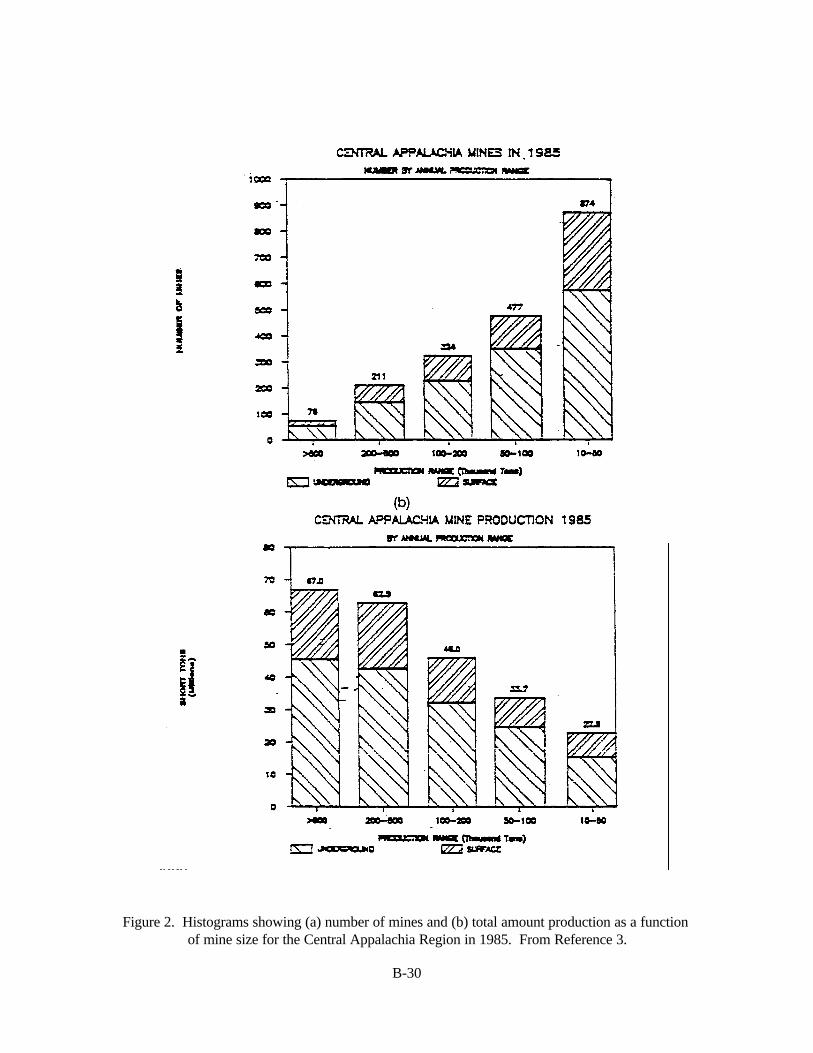
B-30
Figure 2. Histograms showing (a) number of mines and (b) total amount production as a function of mine size for the Central Appalachia Region in 1985. From Reference 3.
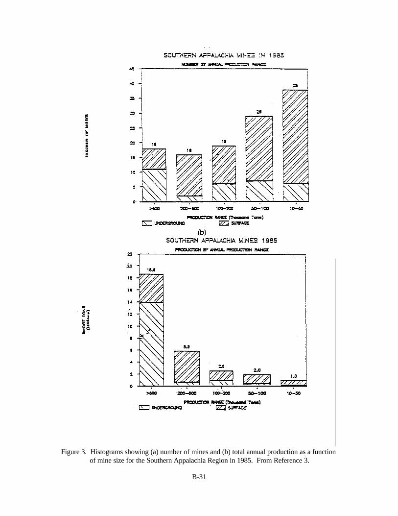
B-31
Figure 3. Histograms showing (a) number of mines and (b) total annual production as a function of mine size for the Southern Appalachia Region in 1985. From Reference 3.

B-32
Figure 4. Histograms showing (a) number of mines and (b) total annual production as a function of mine size for the Midwest Region in 1985. From Reference 3.

B-33
Figure 5. Histograms showing (a) number of mines and (b) total annual production as a functionof mine size for the Powder River Basin in 1985. From Reference 3.

B-34
Figure 6. Histograms showing (a) number of mines and (b) total amount production as a functionof mine size for the Rocky Mountain Region in 1985. From Reference 3.
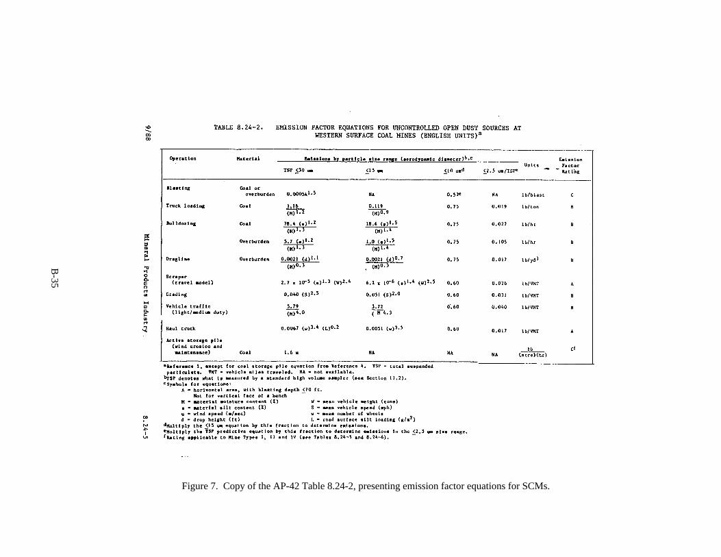
B-35
Figure 7. Copy of the AP-42 Table 8.24-2, presenting emission factor equations for SCMs.
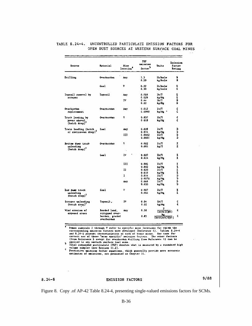
B-36
Figure 8. Copy .of AP-42 Table 8.24-4, presenting single-valued emissions factors for SCMs.

B-37
TABLE 1. EASTERN AND MIDWESTERN UNITED STATES COAL PRODUCTION STATISTICS
Eastern coal production (tons x 103) Average mine size (tons/yr)
Region Total UndergroundPercent oftotal (%) Surface
Percent oftotal (%) Underground Surface
Northern Appalachia 155,532 93,367 60.0 62,165 40.0 472,000 103,000
Central Appalachia 232,380 160,296 69.0 72,083 31.0 127,000 108,000
Southern Appalachia 30,122 16,233 53.9 13,889 46.1 507,000 158,000
Midwest 131,415 57,303 43.6 74,112 56.4 939,000 481,000
Pennsylvania Anthracite 4,281 440 10.3 3,841 89.7 49,000 55,000
Totals 553,730 327,639 59.2 226,091 40.8 -- --
TABLE 2. WESTERN UNITED STATES COAL PRODUCTION STATISTICS
Eastern coal production (tons x 103) Average mine size (tons/yr)
Region Total UndergroundPercent oftotal (%) Surface
Percent oftotal (%) Underground Surface
Rocky Mountain 61,876 19,925 32.2 41,951 67.8 510,000 1,824,000
Powder River Basin 173,997 1,058 0.6 172,939 99.4 1,058,000 4,941,000
Totals 235,873 20,983 8.8 214,890 91.2 -- --

B-38
TABLE 3. SUMMARY OF MAJOR EMISSIONSOURCES AT SURFACE COAL MINES
Topsoil related activities< Removal< Scraper travel< Material handling and storage activities< Replacement
Overburden related activities< Drilling< Blasting<< Removal<< Truck haulage< Material handling and storage activities< Replacement< Dozer activity
Coal seam activities< Drilling< Blasting< Loading< Truck haulage< Truck unloading< Processing (crushing, screening, etc.)< Material handling and storage activities< Dozer activity< Loadout for transit
General activities< Vehicle travel< Road grading< Wind erosion of open areas and materials in storage
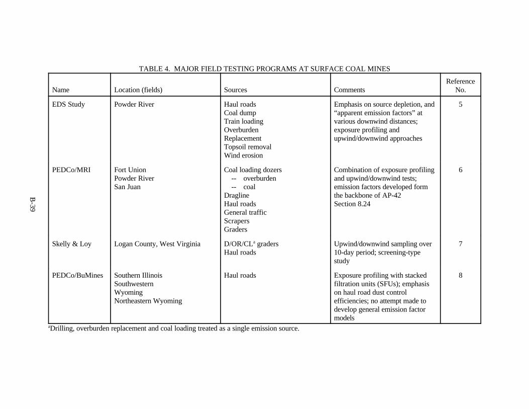
B-39
TABLE 4. MAJOR FIELD TESTING PROGRAMS AT SURFACE COAL MINES
Name Location (fields) Sources CommentsReference
No.
EDS Study Powder River Haul roadsCoal dumpTrain loadingOverburdenReplacementTopsoil removalWind erosion
Emphasis on source depletion, and“apparent emission factors” atvarious downwind distances;exposure profiling andupwind/downwind approaches
5
PEDCo/MRI Fort UnionPowder RiverSan Juan
Coal loading dozers-- overburden-- coal
DraglineHaul roadsGeneral trafficScrapersGraders
Combination of exposure profilingand upwind/downwind tests;emission factors developed formthe backbone of AP-42Section 8.24
6
Skelly & Loy Logan County, West Virginia D/OR/CLa gradersHaul roads
Upwind/downwind sampling over10-day period; screening-typestudy
7
PEDCo/BuMines Southern IllinoisSouthwesternWyomingNortheastern Wyoming
Haul roads Exposure profiling with stackedfiltration units (SFUs); emphasison haul road dust controlefficiencies; no attempt made todevelop general emission factormodels
8
aDrilling, overburden replacement and coal loading treated as a single emission source.
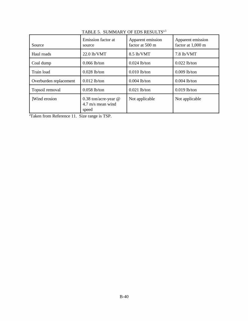
B-40
TABLE 5. SUMMARY OF EDS RESULTSa,5
SourceEmission factor atsource
Apparent emissionfactor at 500 m
Apparent emissionfactor at 1,000 m
Haul roads 22.0 lb/VMT 8.5 lb/VMT 7.8 lb/VMT
Coal dump 0.066 lb/ton 0.024 lb/ton 0.022 lb/ton
Train load 0.028 lb/ton 0.010 lb/ton 0.009 lb/ton
Overburden replacement 0.012 lb/ton 0.004 lb/ton 0.004 lb/ton
Topsoil removal 0.058 lb/ton 0.021 lb/ton 0.019 lb/ton
]Wind erosion 0.38 ton/acre-year @4.7 m/s mean windspeed
Not applicable Not applicable
aTaken from Reference 11. Size range is TSP.
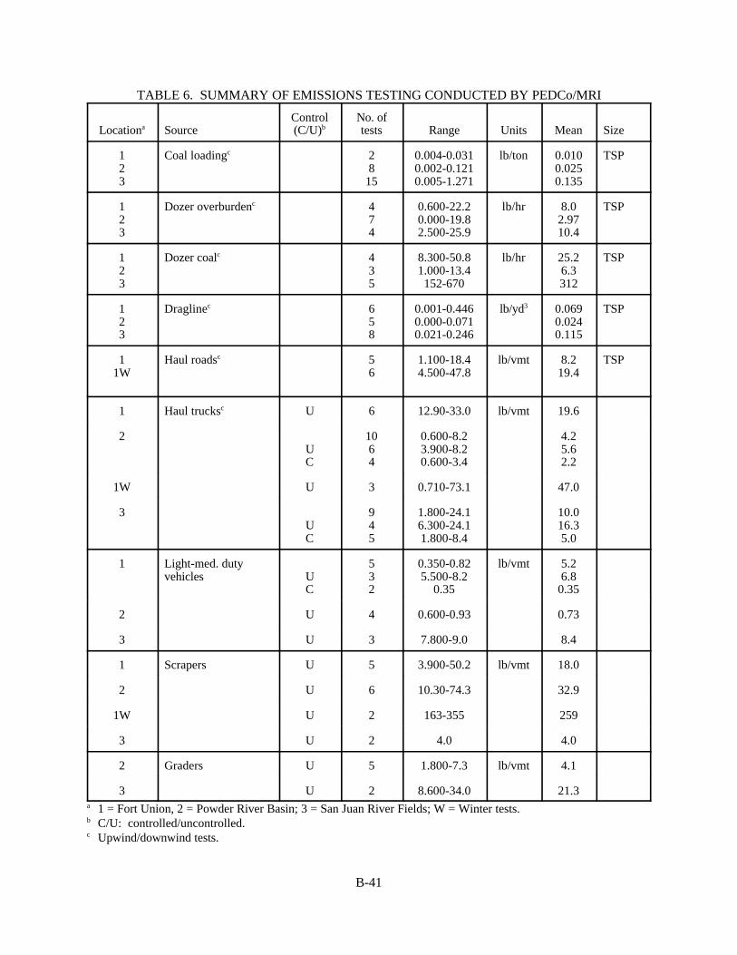
B-41
TABLE 6. SUMMARY OF EMISSIONS TESTING CONDUCTED BY PEDCo/MRI
Locationa SourceControl(C/U)b
No. oftests Range Units Mean Size
123
Coal loadingc 28
15
0.004-0.0310.002-0.1210.005-1.271
lb/ton 0.0100.0250.135
TSP
123
Dozer overburdenc 474
0.600-22.20.000-19.82.500-25.9
lb/hr 8.02.9710.4
TSP
123
Dozer coalc 435
8.300-50.81.000-13.4
152-670
lb/hr 25.26.3312
TSP
123
Draglinec 658
0.001-0.4460.000-0.0710.021-0.246
lb/yd3 0.0690.0240.115
TSP
11W
Haul roadsc 56
1.100-18.44.500-47.8
lb/vmt 8.219.4
TSP
1 Haul trucksc U 6 12.90-33.0 lb/vmt 19.6
2UC
1064
0.600-8.23.900-8.20.600-3.4
4.25.62.2
1W U 3 0.710-73.1 47.0
3UC
945
1.800-24.16.300-24.11.800-8.4
10.016.35.0
1 Light-med. dutyvehicles U
C
532
0.350-0.825.500-8.2
0.35
lb/vmt 5.26.8
0.35
2 U 4 0.600-0.93 0.73
3 U 3 7.800-9.0 8.4
1 Scrapers U 5 3.900-50.2 lb/vmt 18.0
2 U 6 10.30-74.3 32.9
1W U 2 163-355 259
3 U 2 4.0 4.0
2 Graders U 5 1.800-7.3 lb/vmt 4.1
3 U 2 8.600-34.0 21.3a 1 = Fort Union, 2 = Powder River Basin; 3 = San Juan River Fields; W = Winter tests.b C/U: controlled/uncontrolled.c Upwind/downwind tests.
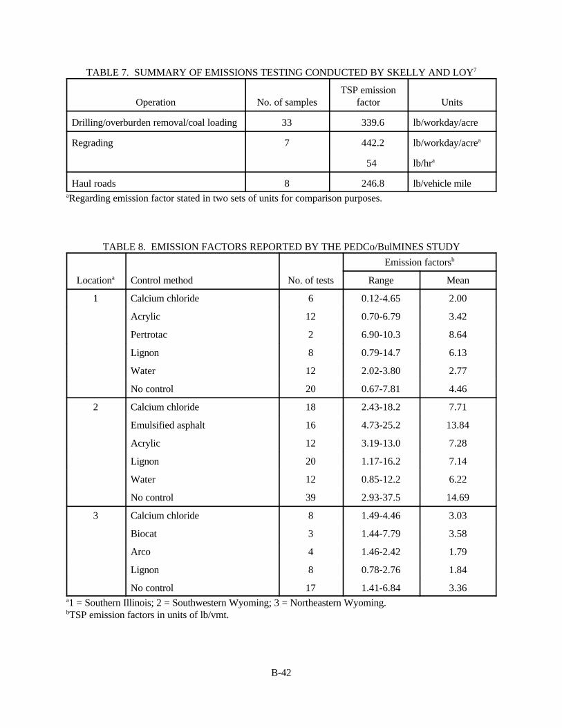
B-42
TABLE 7. SUMMARY OF EMISSIONS TESTING CONDUCTED BY SKELLY AND LOY7
Operation No. of samplesTSP emission
factor Units
Drilling/overburden removal/coal loading 33 339.6 lb/workday/acre
Regrading 7 442.2 lb/workday/acrea
54 lb/hra
Haul roads 8 246.8 lb/vehicle mileaRegarding emission factor stated in two sets of units for comparison purposes.
TABLE 8. EMISSION FACTORS REPORTED BY THE PEDCo/BulMINES STUDY
Locationa Control method No. of tests
Emission factorsb
Range Mean
1 Calcium chloride 6 0.12-4.65 2.00
Acrylic 12 0.70-6.79 3.42
Pertrotac 2 6.90-10.3 8.64
Lignon 8 0.79-14.7 6.13
Water 12 2.02-3.80 2.77
No control 20 0.67-7.81 4.46
2 Calcium chloride 18 2.43-18.2 7.71
Emulsified asphalt 16 4.73-25.2 13.84
Acrylic 12 3.19-13.0 7.28
Lignon 20 1.17-16.2 7.14
Water 12 0.85-12.2 6.22
No control 39 2.93-37.5 14.69
3 Calcium chloride 8 1.49-4.46 3.03
Biocat 3 1.44-7.79 3.58
Arco 4 1.46-2.42 1.79
Lignon 8 0.78-2.76 1.84
No control 17 1.41-6.84 3.36a1 = Southern Illinois; 2 = Southwestern Wyoming; 3 = Northeastern Wyoming.bTSP emission factors in units of lb/vmt.

B-43
TABLE 9. SUMMARY OF EMISSION FACTOR EQUATIONS FROM SCM’s
No. Source Materiala Equation/Factorb Particle size Units Reference
1.a1.b
Blasting C or OC or O
961 A0.8/D1.8 M0.0005A1.5
TSPTSP
lb/blastlb/blast
PEDCo/MRIAP-42 § 8.24c
2.a2.b2.c2.d
Truck loading CCC or OC
1.16/M1.3
0.089/M0.9
k (0.0032)(U/5)1.3/(M/2)1.4
339.6
TSPPM-10eTSP
lb/tonlb/tonlb/tonlb/workday/acre
PEDCo/MRIAP-42 § 8.24d
AP-42 § 11.2.3Skelly & Loy
3.a3.b3.c3.d3.e
Bulldozing CCOOO
78.4 s1.2/M1.3
14 s1.5/M1.4
5.7 s1.2/M1.3
0.75 s1.5/M1.4
54
TSPPM-10TSPPM-10TSP
lb/hrlb/hrlb/hrlb/hrlb/hr
PEDCo/MRIAP-42 § 8.24d
PEDCo/MRIAP-42 § 8.24d
Skelly & Loy
4.a4.b4.c
Dragline OOO
0.0021 d1.1/M0.3
0.0016 d0.7/M0.3
k(0.0032)(U/5)1.3/(M/2)1.4
TSPPM-10e
lb/yd3
lb/yd3
lb/ton
PEDCo/MRIAP-42 § 8.24d
AP-42 § 11.2.3
5.a5.b5.c
Scrapers in travelmode
2.7 x 10⁻⁵s1.3 W2.4
3.7 x 10⁻⁶ s1.4 W2.5
k(5.9)(s/12)(S/30)(W/3)0.7
(w / 4)p0.5 365
365
−
TSPPM-10f
lb/vmtlb/vmtlb/vmt
PEDCo/MRIAP-42 § 8.24d
AP-42 § 11.2.1
6.a6.b6.c
Grading 0.040 S2.5
0.031 S2.0
54
TSPPM-10TSP
lb/vmtlb/vmtlb/hr
PEDCo/MRIAP-42 § 8.24d
Skelly & Loy
7.a7.b7.c7.d7.e
General traffic 5.79/M4.0
1.9/M4.3
k(5.9)(s/12)(S/30)(W/3)0.7
(w/4)0.5(365-p)/3654.83(S/45)1.50
1.22(S/45)1.89
TSPPM-10f
TSPPM-10
lb/vmtlb/vmtlb/vmt
lb/vmtlb/vmt
PEDCo/MRIAP-42 § 8.24d
AP-42 § 11.2.1
Reference 14Reference 14

B-44
TABLE 9. (continued)
No. Source Materiala Equation/Factorb Particle size Units Reference
8.a8.b8.c8.d
8.e
Haul trucks 0.0067 w3.4 L0.2
0.0031 w3.5
246.8k(5.9)(s/12)(S/30)(W/3)0.7
(w/4)0.5(365-p)/36522.0
TSPPM-10TSPf
TSP
lb/vmtlb/vmtlb/vmtlb/vmt
lb/vmt
PEDCO/MRIAP-42 § 8.24d
Skelly & LoyAP-42 § 11.2.1
TRC/EDSaC = coal O = overburden, T = topsoil.bSymbols used:
A = area blasted, ft2
M = moisture content, %D = blasthole depth, fts = silt content, %U = mean wind speed, mph
W = mean vehicle weight, tonS = mean vehicle speed, mphw = mean number of wheelsL = surface silt loading, g/mp = mean annual number of days with at least 0.01 in. of precipitation
cFactor based on a reexamination of PEDCo/MRI study results.dPM-10 factors based on IP emission factors developed in PEDCo/MRI study.eFor SP, k = 0.74; for PM-10, k = 0.35.fFor SP, k = 0.80; for PM-10, k = 0.36.

B-45
Table 10. AVAILABLE SINGLE-VALUED EMISSION FACTORS
No. Source MaterialaTSP emission
factor Units
1.a Drilling O 1.3 lb/hole
1.b C 0.22b lb/hole
2.a. Topsoil removal by scraper T 0.058 lb/T
2.b T 0.44b lb/T
3.a Overburden replacement O 0.012 lb/T
4.a Truck loading by power shovel (batch drop) O 0.037b lb/t
5.a. Train loading (batch or continuous) C 0.028 lb/T
5.b C 0.0002b lb/T
6.a Dump truck unloading (batch) O 0.002b lb/T
6.b C 0.027b lb/T
6.c C 0.005b lb/T
6.d C 0.020b lb/T
6.e C 0.014b lb/T
6.f C 0.066 lb/T
6.g C 0.007b lb/T
7.a Scraper unloading (batch) T 0.04b lb/T
8.a Wind erosion of exposed areas S 0.38 T/acre-yraO = overburden; C = coal; T = topsoil; S = seeded land, stripped overburden, graded overburden.bFactor restricted to use at certain types of mines (see Roman numerals I through V in Figure 8).
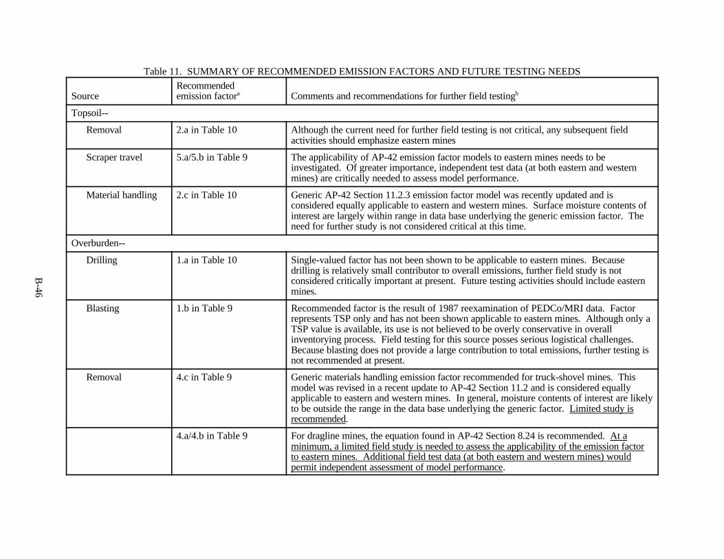
B-46
Table 11. SUMMARY OF RECOMMENDED EMISSION FACTORS AND FUTURE TESTING NEEDS
SourceRecommendedemission factora Comments and recommendations for further field testingb
Topsoil--
Removal 2.a in Table 10 Although the current need for further field testing is not critical, any subsequent fieldactivities should emphasize eastern mines
Scraper travel 5.a/5.b in Table 9 The applicability of AP-42 emission factor models to eastern mines needs to beinvestigated. Of greater importance, independent test data (at both eastern and westernmines) are critically needed to assess model performance.
Material handling 2.c in Table 10 Generic AP-42 Section 11.2.3 emission factor model was recently updated and isconsidered equally applicable to eastern and western mines. Surface moisture contents ofinterest are largely within range in data base underlying the generic emission factor. Theneed for further study is not considered critical at this time.
Overburden--
Drilling 1.a in Table 10 Single-valued factor has not been shown to be applicable to eastern mines. Becausedrilling is relatively small contributor to overall emissions, further field study is notconsidered critically important at present. Future testing activities should include easternmines.
Blasting 1.b in Table 9 Recommended factor is the result of 1987 reexamination of PEDCo/MRI data. Factorrepresents TSP only and has not been shown applicable to eastern mines. Although only aTSP value is available, its use is not believed to be overly conservative in overallinventorying process. Field testing for this source posses serious logistical challenges. Because blasting does not provide a large contribution to total emissions, further testing isnot recommended at present.
Removal 4.c in Table 9 Generic materials handling emission factor recommended for truck-shovel mines. Thismodel was revised in a recent update to AP-42 Section 11.2 and is considered equallyapplicable to eastern and western mines. In general, moisture contents of interest are likelyto be outside the range in the data base underlying the generic factor. Limited study isrecommended.
4.a/4.b in Table 9 For dragline mines, the equation found in AP-42 Section 8.24 is recommended. At aminimum, a limited field study is needed to assess the applicability of the emission factorto eastern mines. Additional field test data (at both eastern and western mines) wouldpermit independent assessment of model performance.

B-47
Table 11. (continued)
SourceRecommendedemission factora Comments and recommendations for further field testingb
Haul trucks 8.a./8.b. in Table 9 Because overburden and coal haul trucks can account for up to half of the total PMemissions, it is important to have an independent assessment of model performance. Thus,collection of new field data at both eastern and western mines should be an importantobjective of any future field effort
Material handling 2.c in Table 10 Generic AP-42 Section 11.2.3 emission factor model was recently updated and isconsidered equally applicable to eastern and western mines. Moisture values are probablyoutside the range of the underlying data base, however. Limited field testingrecommended, in conjunction with other overburden handling operations.
Dozer activity 4.a/4.b in Table 9 At a minimum, the applicability of the emission model to eastern mines should be fieldverified. To facilitate the transfer of results, it is recommended that results be expressedas emission factors rather than emission rates.
Replacement 2.c in Table 9 Because of the importance of this source at truck-shovel mines, further fieldcharacterization (at both eastern and western mines) study is strongly suggested.
Coal--
Drilling 1.b in Table 10 Single-valued factor has not been shown to be applicable to eastern mines. Drilling is arelatively small contributor to overall emissions. Further field study is not consideredcritcally important at this time. Future testing activities should include eastern mines.
Blasting 1.b. in Table 9 TSP factor resulted from 1987 reexamination of PEDCo/MRI data. Has not been shownapplicable to eastern mines. Although only a TSP value is available, its use is not believedto be overly conserative in overall inventorying process. Very difficult source for fieldtesting. Further testing not recommended at present.
Coal loading 2.a./2.b or 2.c in Table 9 Model 2.a/2.b recommended for surface moisture contents greater than 4%, model 2.crecommended for surface moisture contents less than 5%. Because of confusion and/ordebate as to appropriate emission factors and input variables (i.e., surface versus boundmoisture contents) and because of high variability between mines, reexamination of thissource is recommended in future field studies. This testing could be combined with testingof other handling activities (below).
Haul trucks 8.a/8.b in Table 9 Because overburden and coal haul trucks can account for up to half of the total PMemissions, it is important to have an independent assessment of model performance. Thuscollection of new field data at both eastern and western mines should be an importantobjective of any future field effort.

B-48
Table 11. (continued)
SourceRecommendedemission factora Comments and recommendations for further field testingb
Unloading 2.c in Table 10 Generic AP-42 Section 11.2.3 emission factor model was recently updated and isconsidered equally applicable to eastern and western mines. Moisture contents of interestfor coal unloading, however, tend to be far greater than those in generic data base. Limited field testing effort, perhaps focused on eastern mines, is recommended.
Material handling 2.c. in Table 10 Same as previous comment.
Dozer activity 4.a/4.b in Table 9 At a minimum, the applicability of the emission model to eastern mines should be fieldverified. To facilitate the transfer of results, it is recommended that results be expressedas emission factors rather than emission rates.
Loadout for transit 2.c in Table 10 Same as comment for coal unloading.
General--
General traffic 7.c or 7.d/7.e in Table 9 Model 7.d/7.e recommended for light-duty, higher speed traffic in arid portions of thewestern United States. Because general traffic can account for a large portion of the totalPM emissions at a SCM, collection of additional field test data (at both eastern andwestern mines) should be an important objective of any future field effort. Note that, whenapplied to independent data, the light- and medium-duty unpaved road emission model inSection 8.24 overpredicted by one or two orders of magnitude.
Road grading 6.a/6.b in Table 9 Generic unpaved road equation will conservatively overestimate the measured gradingemission factors, and the overestimation is probably not overly restrictive in developing amine-wide PM inventory. Further testing is not critical at present. Future testing ofgraders should emphasize eastern mines.
aEmission factors in bold differ from general guidelines given in Section 8.24 of AP-42.bSuggested field testing underlined.

B-49
SECTION 6
REFERENCES
1. U.S. Environmental Protection Agency, Non-Metallic Mineral Processing Plants, BackgroundInformation for Proposed Standards.
2. Bureau of Mines, Minerals Yearbook (1986), Volume II.
3. Department of Commerce, Coal in the United States, Coal Exporters Association, U.S. Department ofCommerce, International Trade Administration Office of Energy, March 1987.
4. Cole, C. F., B. L. Murphy, J. S. Evans, A. Garsd, Quantification of Uncertainties in EPA's FugitiveEmissions and Modeling Methodologies at Surface Coa/Mines, TRC Environmental Consultants,February 1985.
5. Shearer, D. L., R. A. Dougherty, C. C. Easterbrook, Coal Mining Emission Factor Development andModeling Study, TRC Environmental Consultants, July 1981.
6. U.S. Environmental Protection Agency, Improved Emission Factors for Fugitive Dust from WesternSurface Coal Mining Sources, EPA-600/7-84-048, Two Volumes, March 1984.
7. Ettinger, W. S., and R. E. McClure, Fugitive Dust Generation on a Southern West Virginia SurfaceCoal Mine, APCA Speciality Conference on Fugitive Dust Issues in the Coal Use Cycle, April 1983.
8. Rosenbury, K. D., and R. A. Zimmer, Cost-Effectiveness of Dust Controls Used on Unpaved HaulRoads, Two Volumes, Final Report for U.S. Bureau of Mines, Minneapolis, Minnesota,December 1983.
9. U.S. Environmental Protection Agency, Compilation of Air Pollutant Emission Factors (AP-42),Research Triangle Park, North Carolina, September 1985.
10. Cowherd, C., Jr., and J. S. Kinsey (1986), Identification, Assessment, and Control of FugitiveParticulate Emissions, EPA-600/8-86-023, U.S. Environmental Protection Agency, Washington,D.C.
11. Jacko, R. B., Air Quality, in Surface Mining Environmental Monitoring and ReclamationHandbook, Edited by L.V.A. Sendlein, H. Yazicigili, and C. L. Carlson, Elsevier; New York, 1983.
12. Pyle, B. E., and J. D. McCain, Critical Review of Open Source Particulate Emission Measurements:Part II—Field Comparison, Final Report. Southern Research Institute, Project No. 5050-4, preparedfor the U.S. Environmental Protection Agency, February 1986.
B-50
13. Muleski, G. E., Update of Fugitive Dust Emission Factors in AP-42 Section 11.2, Report for U.S.Environmental Protection Agency, MRI Project No. 8681-L(19), July 1987.
14. Muleski, G. E., Unpaved Road Emission Impact, Report for Arizona Department of EnvironmentalQuality, March 1991.
15. U.S. Environmental Protection Agency, Technical Procedures for Developing AP-42 EmissionFactors and Preparing AP-42 Sections, April 1980.
16. U.S. Environmental Protection Agency, Survey of Fugitive Dust from Coal Mines,EPA-908/1-78-003, February 1978.
17. Muleski, G. E., Update of Fugitive Dust Emission Factors in AP-42, Report for U.S. EnvironmentalProtection Agency, MRI Project No. 8481-L(11), August 1986.
18. Brookman, E. T., D. H. Carnes, P. A. Catizone, K. J. Kelley, Determination of Fugitive Coal DustEmissions from Rotary Railcar Dumping, TRC Environmental Consultants, May 1984.
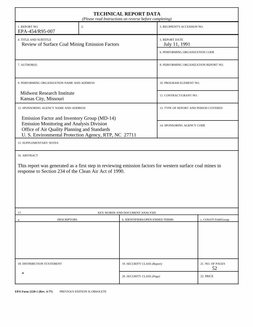
TECHNICAL REPORT DATA(Please read Instructions on reverse before completing)
1. REPORT NO.
EPA-454/R95-0072. 3. RECIPIENT'S ACCESSION NO.
4. TITLE AND SUBTITLE
Review of Surface Coal Mining Emission Factors5. REPORT DATE
July 11, 1991
6. PERFORMING ORGANIZATION CODE
7. AUTHOR(S)
8. PERFORMING ORGANIZATION REPORT NO.
9. PERFORMING ORGANIZATION NAME AND ADDRESS
Midwest Research Institute Kansas City, Missouri
10. PROGRAM ELEMENT NO.
11. CONTRACT/GRANT NO.
12. SPONSORING AGENCY NAME AND ADDRESS
Emission Factor and Inventory Group (MD-14) Emission Monitoring and Analysis Division Office of Air Quality Planning and Standards U. S. Environmental Protection Agency, RTP, NC 27711
13. TYPE OF REPORT AND PERIOD COVERED
14. SPONSORING AGENCY CODE
15. SUPPLEMENTARY NOTES
16. ABSTRACT
This report was generated as a first step in reviewing emission factors for western surface coal mines inresponse to Section 234 of the Clean Air Act of 1990.
17. KEY WORDS AND DOCUMENT ANALYSIS
a. DESCRIPTORS b. IDENTIFIERS/OPEN ENDED TERMS c. COSATI Field/Group
18. DISTRIBUTION STATEMENT
*
19. SECURITY CLASS (Report) 21. NO. OF PAGES
52
20. SECURITY CLASS (Page) 22. PRICE
EPA Form 2220-1 (Rev. 4-77) PREVIOUS EDITION IS OBSOLETE

C-1
Appendix CSampling Methodology
This appendix contains information on methods of sampling fugitive dust emissions. The
information found in this appendix is from Section 4.2 of the EPA report “Fugitive Dust Emission Factor
Update for AP-42 ” and Section 3 of the EPA report “Improved Emission Factors For Fugitive Dust From
Western Surface Coal Mining Sources - Volume I - Sampling Methodology and Test Results.”

C-2
TABLE OF CONTENTS
Page
C.1 Section 4.2 of Report: "Fugitive Dust Emission Factor Update for AP-42." . . . . . . . . . . . . . C-3
C.2 Section 3 of Report: "Improved Emission Factors for Fugitive Dust From Western Surface Coal Mining Sources--Volume 1 - Sampling Methodology and Test Results." . . . . . . . . . . . . . . . . . . . . . . . . . . . . . . . . . . . . . . . . . . . . . . . . . . . . . . . . C-8

C-3
C.1 Section 4.2 of Report: "Fugitive Dust Emission Factor Update for AP-42."
4.2 Methods of Emission Factor Determination
Fugitive dust emission rates and particle size distributions are difficult to quantify because of thediffuse and variable nature of such sources and the wide range of particle size involved including particleswhich deposit immediately adjacent to the source. Standard source testing methods, which are designed forapplication to confined flows under steadystate, forced-flow conditions, are not suitable for measurementof fugitive emissions unless the plume can be drawn into a forced-flow system.
Mass Emissions Measurement
For field measurement of fugitive mass emissions, three basic techniques have been defined(Development of Procedures for Measurement of Fugitive Emissions, EPA-600/2-76-284) which aresummarized as follows:
1. The quasi-stack method involves capturing the entire emissions stream with enclosures orhoods and applying conventional source testing techniques to the confined flow.
2. The roof monitor method involves measurement of concentrations and airflows across welldefined building openings such as roof monitors, ceiling vents, and windows.
3. The upwind-downwind method involves measurement of upwind and downwind air quality,utilizing ground based samplers under known meteorological conditions, and calculation of source strengthwith atmospheric dispersion equations.
Because it is impractical to enclose open dust sources or to capture the entire emissions plume, theupwind-downwind method is the only one of these three that is suitable for measurement of particulateemissions from open dust sources.
The basic procedure of the upwind-downwind method involves the measurement of particulateconcentrations both upwind and downwind of the pollutant source. The number of upwind samplinginstruments depend on the isolability of the source operation of concern (i.e., the absence of interferencefrom other sources upwind). Increasing the number of downwind instruments improves the reliability indetermining the emission rate by providing better plume definition. In order to reasonably define the plumeemanating from a point source, instruments need to be located at two downwind distances and threecrosswind distances at a minimum. The same sampling requirements pertain to line sources except thatmeasurement need not be made at multiple crosswind distances.
After the concentration(s) measured upwind are subtracted from the downwind concentrations, thenet downwind concentrations are then used as input to dispersion equations (normally of the Gaussiantype) to back calculate the particulate emission rate required to generate the downwind pollutantconcentration measured. A number of meteorological parameters must be concurrently recorded for inputto this dispersion equation. At a minimum the wind direction and speed must be recorded on-site.

C-4
While the upwind-downwind method is applicable to virtually all types of sources, it hassignificant limitations with regard to development of source-specific emission factors. The majorlimitations are as follows:
1. In attempting to quantify a large area source, overlapping of plumes from upwind(background) sources may preclude the determination of the specific contribution of the area source.
2. Because of the impracticality of adjusting the locations of the sampling array for shifts in winddirection during sampling, it cannot be assumed that plume position is fixed in the application of thedispersion model.
3. The usual assumption that an area source is uniformly emitting does not allow for realisticrepresentation of spatial variation in source activity.
4. The typical use of uncalibrated atmospheric dispersion models introduces the possibility ofsubstantial error (a factor of three according to Turner, 1970) in the calculated emission rate, even if thestringent requirement of unobstructed dispersion from a simplified source configuration is met.
Two additional measurement techniques, exposure profiling and the wind tunnel method offerdistinct advantages for source-specific quantification of fugitive emissions from open dust sources.
The exposure profiling technique uses the isokinetic profiling concept that is the basis forconventional (ducted) source testing. The passage of airborne pollutant immediately downwind of thesource is measured directly by means of simultaneous multipoint sampling over the effective cross sectionof the fugitive emissions plume. This technique uses a mass-balance calculation scheme similar to EPAMethod 5 stack testing rather than requiring indirect calculation through the application of a generalizedatmospheric dispersion model.
For measurement of nonbuoyant fugitive emissions, profiling sampling heads are distributed overa vertical network positioned just downwind (usually about 5 m) from the source. If total particulateemissions are measured, sampling intakes are pointed into the wind and sampling velocity is adjusted tomatch the local mean wind speed, as monitored by distributed anemometers.
The size of the sampling grid needed for exposure profiling of a particular source may beestimated by observation of the visible size of the plume or by calculation of plume dispersion. Grid sizeadjustments may be required based on the results of preliminary testing. Particulate sampling heads shouldbe symmetrically distributed over the concentrated portion of the plume containing about 90% of the totalmass flux (exposure). For example, assuming that the exposure from a point source is normally dis-tributed, the exposure values measured by the samplers at the edge of the grid should be about 25% of thecenterline exposure.
To calculate emission rates using the exposure profiling technique, a conservation of massapproach is used. The passage of airborne particulate, i.e., the quantity of emissions per unit of sourceactivity, is obtained by spatial integration of distributed measurements of exposure (mass/area) over theeffective cross section of the plume. The exposure is the point value of the flux (mass/area-time) ofairborne particulate integrated over the time of measurement. The steps in the calculation procedure arepresented in the paragraphs below.
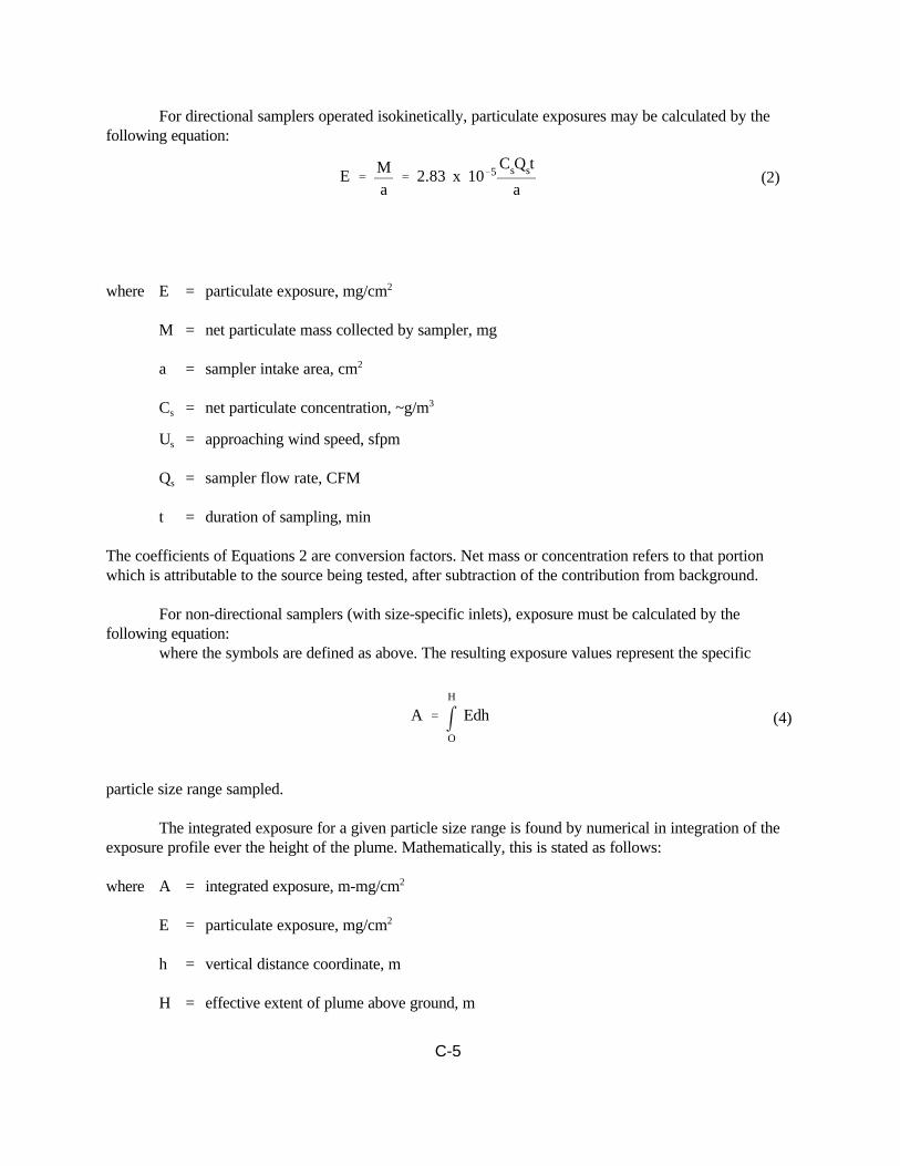
C-5
E 'Ma
' 2.83 x 10&5CsQst
a(2)
A ' mH
O
Edh (4)
For directional samplers operated isokinetically, particulate exposures may be calculated by thefollowing equation:
where E = particulate exposure, mg/cm2
M = net particulate mass collected by sampler, mg
a = sampler intake area, cm2
Cs = net particulate concentration, ~g/m3
Us = approaching wind speed, sfpm
Qs = sampler flow rate, CFM
t = duration of sampling, min
The coefficients of Equations 2 are conversion factors. Net mass or concentration refers to that portionwhich is attributable to the source being tested, after subtraction of the contribution from background.
For non-directional samplers (with size-specific inlets), exposure must be calculated by thefollowing equation:
where the symbols are defined as above. The resulting exposure values represent the specific
particle size range sampled.
The integrated exposure for a given particle size range is found by numerical in integration of theexposure profile ever the height of the plume. Mathematically, this is stated as follows:
where A = integrated exposure, m-mg/cm2
E = particulate exposure, mg/cm2
h = vertical distance coordinate, m
H = effective extent of plume above ground, m

C-6
Physically, A represents the total passage of airborne particulate matter downwind of the source, per unitlength of line source.
The wind tunnel method utilizes a portable pull-through wind tunnel with an open-floored testsection placed directly over the surface to be tested. Air is drawn through the tunnel at controlledvelocities. The exit air stream from the test section passes through a circular duct fitted with an isokineticprobe at the downstream end. Air is drawn through the probe by a high-volume sampling train. Thistechnique provides for precise study of the wind erosion process with minimal interference frombackground sources.
Particle Sizing
High-volume cascade impactors with glass fiber impaction substrates, which are commonly usedto measure mass size distribution of atmospheric particulate, may be adapted for sizing of fugitiveparticulate emissions. A cyclone preseparator (or other device) is needed to remove coarse particles whichotherwise would be subject to particle bounce within the impactor causing fine particle bias. Once again,the sampling intake should be pointed into the wind and the sampling velocity adjusted to the mean localwind speed by fitting the intake with a nozzle of appropriate size.
The recently developed EPA version of the dichotomous sampler, which is virtually free of particlebounce problems is useful for quantification of fine particle mass concentrations. However, this deviceoperates at a low flow rate (1 cu m/hr) yielding only 0.024 mg of sample in 24 hr for each 10 Fg/m3 ofTSP concentration. Thus, an analytical balance of high precision is required to determine massconcentrations below and above the fine particulate (2.5 Fm) cutpoint (the minimum in the typical bimodalsize distribution of atmospheric particulate). In addition, the dichotomous sampler was designed to have a15 Fm cutpoint for capture of airborne particles (the upper size limit for inhalable particulate based onunit density); however, recent wind tunnel studies have shown that this cutpoint is wind sensitive(Wedding, 1980).
The size-selective inlet for a standard high-volume sampler is also designed to capture particulatematter smaller than 15 Fm in aerodynamic diameter. This unit is much less wind sensitive than thedichotomous sampler but it does not provide a cutpoint at 2.5 Fm. However, it can be adapted for use witha high volume cascade impactor to define a mass size distribution of smaller than 15 Fm in diameter.Recently, size-specific inlets with 10 Fm cutpoints have become available for both dichotomous samplersand high-volume samplers.
Emission Factor Derivation
Usually the final emission factor for a given source operation, as presented in a test report, isderived simply as the arithmetic average of the individual emission factors calculated from each test of thatsource. Frequently the range of individual emission factor values is also presented.
As an alternative to the presentation of a final emission factor as a single-valued arithmetic mean,an emission factor may be presented in the form of a predictive equation derived by regression analysis oftest data. Such an equation mathematically relates emissions to parameters which characterize sourceconditions. These parameters may be grouped into three categories:
C-7
1. Measures of sources activity or energy expended (for example, the speed and weight of avehicle traveling on an unpaved road).
2. Properties of the material being disturbed (for example, the content of suspendable fines in thesurface material on an unpaved road).
3. Climatic parameters (for example, number of precipitation-free days per year on whichemissions tend to be at a maximum).
An emission factor equation is useful if it is successful in “explaining” much of the observedvariance in emission factor values on the basis of corresponding variances in specific source parameters.This enables more reliable estimates of source emissions on a site-specific basis.
A generic emission factor equation is one that is developed for a source operation defined on thebasis of a single dust generation mechanism which crosses industry lines. An example would be vehiculartraffic on unpaved roads. To establish its applicability, a generic equation should be developed from testdata obtained in different industries.
C-8
C.2 Section 3 of Report: "Improved Emission Factors for Fugitive Dust From Western Surface CoalMining Sources--Volume 1 - Sampling Methodology and Test Results."
SECTION 3SAMPLING METHODOLOGY
TECHNIQUES AVAILABLE TO SAMPLE FUGITIVE DUST EMISSIONS
Five basic techniques have been used to measure fugitive dust emissions. These are quasi-stack,roof monitor, exposure profiling, upwind-downwind and wind tunnel. Several experimental samplingmethods are in developmental stages.
In the quasi-stack method of sampling, the emissions from a well-defined process are captured in atemporary enclosure and vented to a duct or stack of regular cross-sectional area. The emissionconcentration and the flow rate of the air stream in the duct are measured using standard stack sampling orother conventional methods.
Roof monitor sampling is used to measure fugitive emissions entering the ambient air frombuildings or other enclosure openings. This type of sampling is applicable to roof vents, doors, windows,or numerous other openings located in such fashion that they prevent the installation of temporaryenclosures.
The exposure profiling technique employs a single profile tower with multiple sampling heads toperform simultaneous multipoint isokinetic sampling over the plume cross-section. The profiling tower is 4to 6 meters in height and is located downwind and as close to the source as possible (usually 5 meters).This method uses monitors located directly upwind to determine the background contribution. Amodification of this technique employs balloon-suspended samplers.
With the upwind-downwind technique, an array of samplers is set up both upwind and downwindof the source. The source contribution is determined to be the difference between the upwind anddownwind concentrations. The resulting contribution is then used in standard dispersion equations to back-calculate the source strength.
The wind tunnel method utilizes a portable wind tunnel with an open-floored test section placeddirectly over the surface to be tested. Air is drawn through the tunnel at controlled velocities. A probe islocated at the end of the test section and the air is drawn through a sampling train.
Several sampling methods using new sampling equipment or sampling arrays are in various stagesof development. These include tracer studies, lidar, acoustic radar, photometers, quartz crystal impactors,etc.
SELECTION OF SAMPLING METHODS
Each of the five basic techniques used to measure fugitive dust emissions has inherent advantages,disadvantages, and limitations to its use.
C-9
The quasi-stack method is the most accurate of the airborne fugitive emission sampling techniquesbecause it captures virtually all of the emissions from a given source and conveys them to a measurementlocation with minimal dilution (Kalika et al. 1976). Its use is restricted to emission sources that can beisolated and are arranged to permit the capture of the emissions. There are no reported uses of thistechnique for sampling open sources at mines.
The roof monitor method is not as accurate as the quasi-stack method because a significantportion of the emissions escape through other openings and a higher degree of dilution occurs beforemeasurement. This method can be used to measure many indoor sources where emissions are released tothe ambient air at low air velocities through large openings. With the exception of the preparation plantand enclosed storage, none of the sources at mines occur within buildings.
The exposure profiling technique is applicable to sources where the ground-based profiler towercan be located vertically across the plume and where the distance from the source to the profiling towercan remain fixed at about 5 meters. This limits application to point sources and line sources. An exampleof a line source that can be sampled with this technique is haul trucks operating on a haul road. Sourcessuch as draglines cannot be sampled using this technique because the source works in a general area(distance between source and tower cannot be fixed), and because of sampling equipment and personnelsafety.
The upwind-downwind method is the least accurate of the methods described because only a smallportion of the emissions are captured in the highly diluted transport air stream (Kalika et al. 1976). It is,however, a universally applicable method. It can be used to quantify emissions from a variety of sourceswhere the requirements of exposure profiling cannot be met.
The wind tunnel method has been used to measure wind erosion of soil surfaces and coal piles(Gillette 1978; Cowherd et al. 1979). It offers the advantages of measurement of wind erosionunder controlled wind conditions. The flow field in the tunnel has been shown to adequately simulate theproperties of ambient winds which entrain particles from erodible surfaces (Gillette 1978).
Experimental sampling methods present at least three problems for coal mine applications. First,none have been used in coal mines to date. Second, they are still in experimental stages, so considerabletime would be required for testing and development of standard operating procedures. Third, the persample costs would be considerably higher than for currently available sampling techniques, thus reducingthe number of samples that could be obtained. Therefore, these techniques were not considered applicablemethods for this study.
After review of the inherent advantages, disadvantages and limitations of each of the five basicsampling techniques, the basic task was to determine which sampling method was most applicable to thespecific sources to be sampled, and whether that method could be adapted to meet the multiple objectivesof the study and the practical constraints of sampling in a surface coal mine.
Drilling was the only source which could be sampled with the quasi-stack method. No roofmonitor sampling could be performed because none of the sources to be sampled occurs within a building.It was decided that the primary sampling method of the study would be exposure profiling. The decisionwas based primarily on the theoretically greater accuracy of the profiling technique as opposed to upwind-downwind sampling and its previous use in similar applications. Where the constraints of exposure

C-10
profiling could not be met (point sources with too large a cross-sectional area), upwind-downwind wouldbe used. The wind tunnel would be used for wind erosion sampling.
SAMPLING CONFIGURATIONS
Basic Configurations
Exposure Profiling--
Source strength--The exposure profiler consisted of a portable tower, 4 to 6 m in height,supporting an array of sampling heads. Each sampling head was operated as an isokinetic exposuresampler. The air flow stream passed through a settling chamber sampler. The air flow stream passedthrough a settling chamber (trapping particles larger than about 50 Fm in diameter), and then flowedupward through a standard 8 in. x 10 in. glass fiber filter positioned horizontally. Sampling intakes werepointed into the wind, and the sampling velocity of each intake was adjusted to match the local mean windspeed as determined prior to each test. Throughout each test, wind speed was monitored by recordinganemometers at two heights, and the vertical wind speed profile was determined by assuming a logarithmicdistribution. This distribution has been found to describe surface winds under neutral atmosphericstability, and is a good approximation for other stability classes over the short vertical distances separatingthe profiler samples (Cowherd, Axetell, Guenther, and Jutze 1974). Sampling time was adequate toprovide sufficient particulate mass ($10 mg) and to average over several units of cyclic fluctuation in theemission rate (e.g., vehicle passes on an unpaved road). A diagram of the profiling tower appears in Figure3-1.
The devices used in the exposure profiling tests to measure concentrations and/or fluxes ofairborne particulate matter are listed in Table 3-1. Note that only the (isokinetic) profiling samplersdirectly measure particulate exposure (mass per unit intake area) as well as particulate concentration(mass per unit volume). However, in the case of the other sampling devices, exposure may be calculated asthe product of concentration, mean wind speed at the height of the sampler intake, and sampling time.
Two deployments of sampling equipment were used in this study: the basic deployment describedin Table 3-2 and the special deployment shown in Table 3-3 for the comparability study.
Particle size--Two Sierra dichotomous samplers, a standard hi-vol, and a Sierra cascade impactorwere used to measure particle sizes downwind. The dichotomous samplers collected fine and coarsefractions with upper cut points (50 percent efficiency) of 2.5 Fm and approximately 15 Fm. (Adjustmentsfor wind speed sensitivity of the 15 Fm cut point are discussed in Section 5; limitations of this samplingtechnique are described on Pages 12-4 and 12-5.)
The high-volume parallel-slot cascade impactor with a 20 cfm flow controller was equipped with aSierra cyclone preseparator to remove coarse particles that otherwise would tend to bounce off the glassfiber impaction substrates. The bounce-through of coarse particles produces an excess of catch on thebackup filter. This results in a positive bias in the measurement of fine particles (see Page 6-3). Thecyclone sampling intake was directed into the wind and the sampling velocity adjusted to mean wind speedby fitting the intake with a nozzle of appropriate size, resulting in isokinetic sampling for wind speedsranging from 5 to 15 mph.
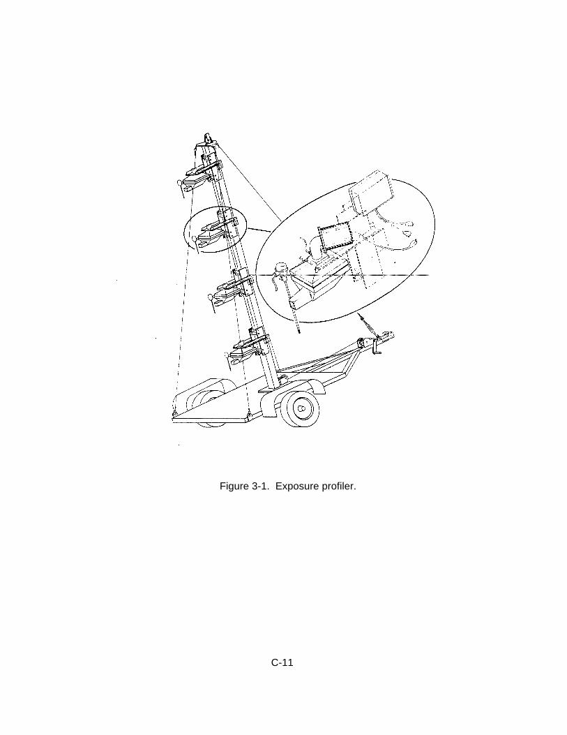
C-11
Figure 3-1. Exposure profiler.
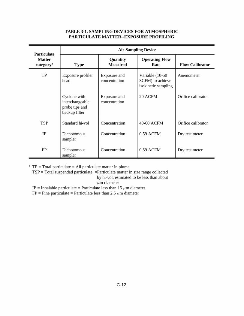
C-12
TABLE 3-1. SAMPLING DEVICES FOR ATMOSPHERICPARTICULATE MATTER--EXPOSURE PROFILING
ParticulateMatter
categorya
Air Sampling Device
TypeQuantityMeasured
Operating FlowRate Flow Calibrator
TP Exposure profilerhead
Exposure andconcentration
Variable (10-50SCFM) to achieveisokinetic sampling
Anemometer
Cyclone withinterchangeableprobe tips andbackup filter
Exposure andconcentration
20 ACFM Orifice calibrator
TSP Standard hi-vol Concentration 40-60 ACFM Orifice calibrator
IP Dichotomoussampler
Concentration 0.59 ACFM Dry test meter
FP Dichotomoussampler
Concentration 0.59 ACFM Dry test meter
a TP = Total particulate = All particulate matter in plumeTSP = Total suspended particulate =Particulate matter in size range collected
by hi-vol, estimated to be less than aboutFm diameter
IP = Inhalable particulate = Particulate less than 15 Fm diameterFP = Fine particulate = Particulate less than 2.5 Fm diameter

C-13
TABLE 3-2. BASIC EQUIPMENT DEPLOYMENT FOR EXPOSURE PROFILING
LocationDistance from
Source (m) Equipment Intake Height (m)a
Upwind 5 1 Dichotomous sampler1 Standard hi-vol2 Dustfall buckets1 Continuous wind monitor
2.52.50.754.0
Downwind 5-10 1 MRI exposure profiler with 4sampling heads
1.53.04.56.0
(1.0)(2.0)(3.0)(4.0)
1 Standard hi-vol1 Hi-vol with cascade impactor2 Dichotomous samplers
2.52.51.54.5
(2.0)(2.0)
(3.0)
2 Dustfall buckets2 Warm wire anemometers
0.751.54.5
(1.0)(3.0)
Downwind 20 2 Dustfall buckets 0.75
Downwind 50 2 Dustfall buckets 0.75
a Alternative heights for sources generating lower plume heights are given in parentheses.

C-14
TABLE 3-3. SPECIAL EQUIPMENT DEPLOYMENT FOR EXPOSUREPROFILING--COMPARABILITY TESTS
LocationDistance from
Source (m) Equipment
IntakeHeight
(m)a
Upwind 5-10 1 Standard hi-vol1 Standard hi-vol2 Dustfall buckets1 Continuous wind monitor
1.252.50.754.0
Downwind 5 1 MRI exposure profiler with 4sampling heads
1 Standard hi-vol2 Hi-vols with cascade impactors
1.53.04.56.02.51.5
4 Dichotomous samplers
2 Dustfall buckets2 Warm wire anemometers
1.53.04.56.00.751.54.5
Downwind 20 1 Hi-vol with cascade impactor2 Dustfall buckets
2.50.75
Downwind 50 2 Dustfall buckets 0.75
Figure 3-2. Upwind-downwind sampling array.Figure 3-3. Wind tunnel.Figure 3-4. Quasi-stack sampling--temporary enclosure for drill sampling.

C-15
Deposition--Particle deposition was measured by placing dustfall buckets along a line downwindof the source at distances of 5 m, 20 m, and 50 m from the source. Greater distances would have beendesirable for establishing the deposition curve, but measurable weights of dustfall could not be obtained beyond about 50 m during the 1-hour test periods. Dustfall buckets were collocated at each distance. Thebucket openings were located 0.75 m above ground to avoid the impact of saltating particles generated bywind erosion downwind of the source.
Exposure Profiling Modification for Sampling Blasts--
Source strength--The exposure profiler concept was modified for sampling blasts. The largehorizontal and vertical dimensions of the plumes necessitated a suspended array of samplers as well asground-based samplers in order to sample over the plume cross-section in two dimensions. Five 47 mmPVC filter heads and sampling orifices were attached to a line suspended from a tethered balloon. Thesamplers were located at five heights with the highest at 30.5 m (2.5, 7.6, 15.2, 22.9, and 30.5 m). Eachsampler was attached to a wind vane so that the orifices would face directly into the wind. The samplerswere connected to a ground based pump with flexible tubing. The pump maintained an isokinetic flow ratefor a wind speed of 5 mph. In order to avoid equipment damage from the blast debris and to obtain arepresentative sample of the plume, the balloon-suspended samplers were located about 100 m downwindof the blast area. This distance varied depending on the size of the blast and physical constraints. Thedistance was measured with a tape measure. The balloon-supported samplers were supplemented with fivehi-vol/dichot pairs located on an arc at the same distance as the balloon from the edge of the blast area,and were spaced 20 m apart.
Particle size--The five ground-based dichotomous samplers provided the basic particle sizeinformation.
Deposition--There was no measurement of deposition with this sampling method. Dustfall sampleswould have been biased by falling debris from the blast.
Upwind-Downwind--
Source strength--The total upwind-downwind array used for sampling point sources included 15samplers, of which 10 were hi-vols and 5 were dichotomous samplers. The arrangement is shownschematically in Figure 3-2. The downwind distances of the samplers from point sources were nominally30 m, 60 m, 100 m, and 200 m. Frequently, distances in the array had to be modified because of physicalobstructions (e.g., highwall) or potential interfering sources. A tape measure was used to measure source--to-sampler distances. The upwind samplers were placed 30 to 100 m upwind, depending on accessibility.The hi-vol and dichotomous samplers were mounted on tripod stands at a height of 2.5 m. This was thehighest manageable height for this type of rapid-mount stand.
This array was modified slightly when sampling line sources. The array consisted of two hi-vol/dichot pairs at 5 m, 20 m, and 50 m with 2 hi-vols at 100 m. The two rows of samplers were normallyseparated by 20 m.
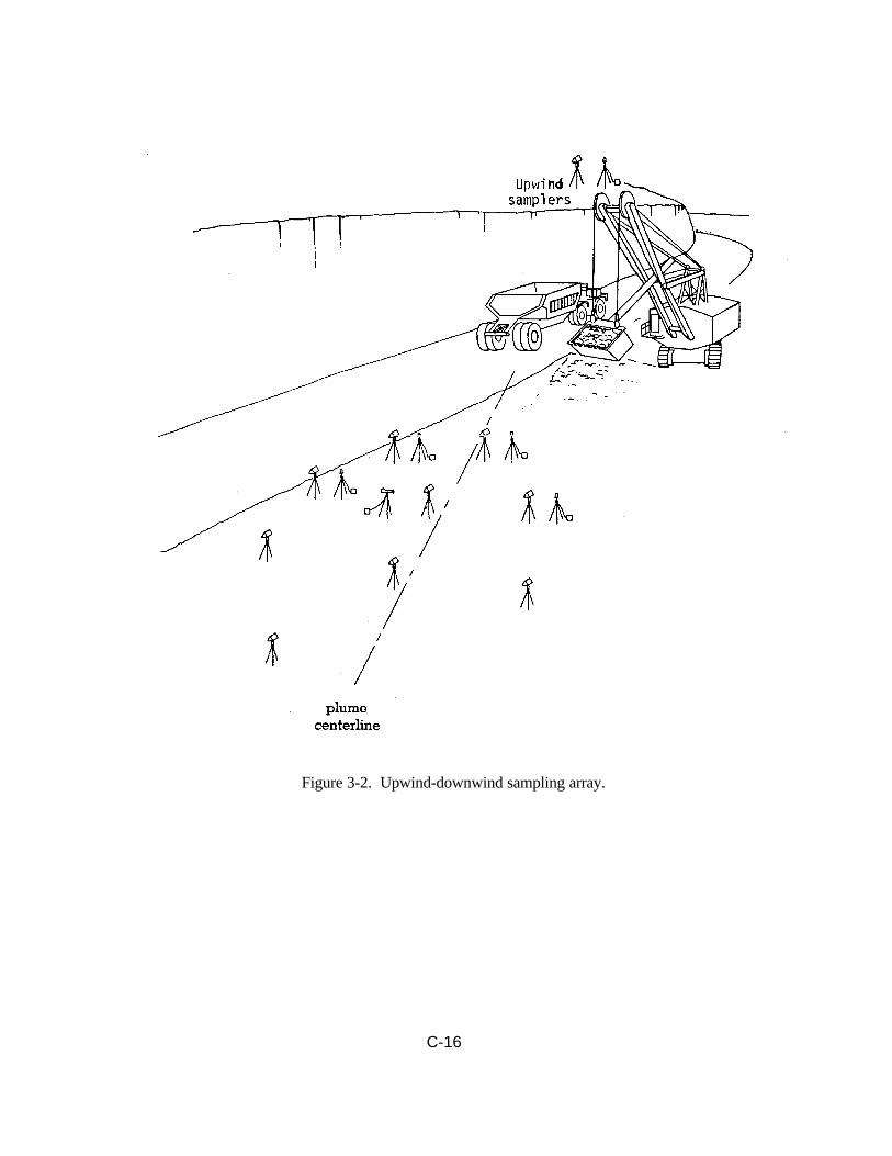
C-16
Figure 3-2. Upwind-downwind sampling array.

C-17
Particle size--In addition to the dichotomous samplers located upwind of the source and at 30 mand 60 m distances downwind of the source, millipore filters were exposed for shorter time periods duringthe sampling at different downwind distances. These filters were to be subjected to microscopicexamination for sizing, but most of this work was suspended because of poor agreement of microscopywith aerodynamic sizing methods in the comparability study.
Deposition--The upwind-downwind method allows indirect measurement of deposition throughcalculation of apparent emission rates at different downwind distances. The reduction in apparent emissionrates as a function of distance is attributed to deposition. At distances beyond about 100 m, depositionrates determined by this method would probably be too small to be detectedseparate from plume dispersion.
Wind Tunnel--
Source strength--For the measurement of dust emissions generated by wind erosion of exposedareas and storage piles, a portable wind tunnel was used. The tunnel consisted of an inlet section, a testsection, and an outlet diffuser. As a modification to previous wind tunnel designs, the working section hada 1 foot by 1 foot cross section. This enlargement was made so that the tunnel could be used with roughersurfaces. The open-floored test section of the tunnel was placed directly on the surface to be tested (1 ft x8 ft), and the tunnel air flow was adjusted to predetermined values that corresponded to the means of theupper NOAA wind speed ranges. Tunnel wind speed was measured by a pitot tube at the downstream endof the test section. Tunnel wind speeds were related to wind speed at the standard 10 m height by means ofa logarithmic profile.
An airtight seal was maintained along the sides of the tunnel by rubber flaps attached to thebottom edges of the tunnel sides. These were covered with material from areas adjacent to the test surfaceto eliminate air infiltration.
To reduce the dust levels in the tunnel air intake stream, testing was conducted only when ambientwinds were well below the threshold velocity for erosion of the exposed material. A portable high-volumesampler with an open-faced filter (roof structure removed) was operated on top of the inlet section tomeasure background dust levels. The filter was vertically oriented parallel to the tunnel inlet face.
An emission sampling module was used with the pull-through wind tunnel in measuring particulateemissions generated by wind erosion. As shown in Figure 3-3, the sampling module was located betweenthe tunnel outlet hose and the fan inlet. The sampling train, which was operated at 15-25 cfm, consisted ofa tapered probe, cyclone precollector, parallel-slot cascade impactor, backup filter, and high-volumemotor. Interchangeable probe tips were sized for isokinetic sampling over the desired tunnel wind speedrange. The emission sampling train and the portable hi-vol were calibrated in the field prior to testing.
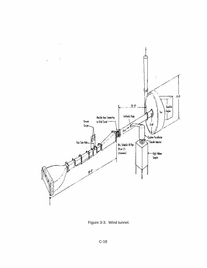
C-18
Figure 3-3. Wind tunnel.

C-19
Particle size--The size distribution for 30 Fm and smaller particles was generated from thecascade impactor used as the total particulate sampler. The procedure for correction of the size data toaccount for particle bounce-through is described in Section 5.
Deposition--No method of measuring the deposition rate of particles suspended by wind erosion inthe test section could be incorporated into the design of the wind tunnel.
Quasi-Stack--
Source strength--An enclosure was fabricated consisting of an adjustable metal frame coveredwith plastic. The frame was 6 feet long with maximum openings at the ends of 5 x 6 feet. Due to problemswith the plastic during high winds, the original enclosure was replaced with a wood enclosure withopenings 4 x 6 feet, as shown in Figure 3-4. For each test, the enclosure was placed downwind of the drillbase. The outlet area was divided into four rectangles of equal area, and the wind velocity was measured atthe center of each rectangle with a hot wire anemometer to define the wind profile inside the frame.
Four exposure profiler samplers with flow controllers were used to sample the plume. Using thewind profile data, the sampler flow rates were adjusted at 2 to 3 minute intervals to near-isokineticconditions.
Particle size--The only particle size measurements made with this sampling method was the splitbetween the filter catch and settling chamber catch in the profiler heads.
Deposition--There was no direct measurement of deposition with this sampling method.
Sampling Configurations by Source
The basic sampling configurations were adapted to each source to be tested. Samplingconfigurations used for each source are indicated in Table 3-4 and described below.
Overburden Drilling--
This activity was sampled using the quasi-stack configuration.
Blasting--
The plume from a blast is particularly difficult to sample because of the vertical and horizontaldimensions of the plume and the inability to place sampling equipment near the blast. Further, the plume issuspected to be non-Gaussian because of the way in which the plume is initially formed. Therefore,upwind-downwind sampling is not appropriate. To sample blasts, a modification of the exposure profilingtechnique was developed. This modification was discussed previously. A typical sampling array is shownin Figure 3-5. The same sampling procedure was used for overburden blasts and coal blasts.
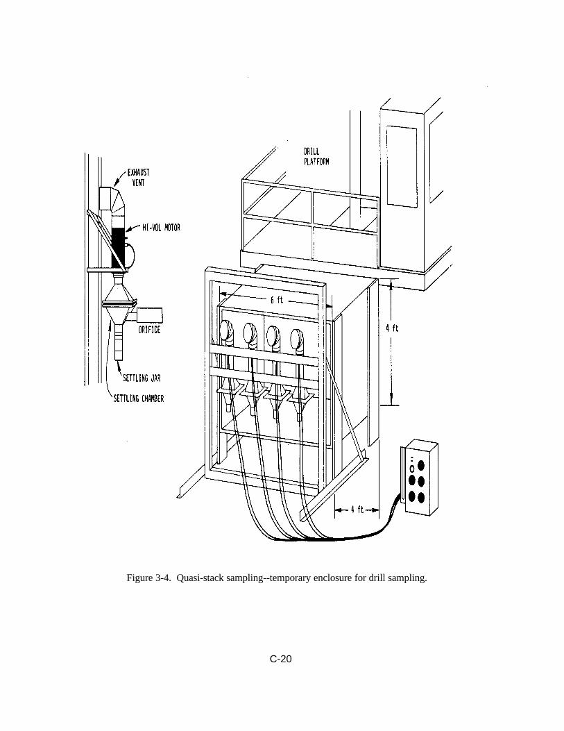
C-20
Figure 3-4. Quasi-stack sampling--temporary enclosure for drill sampling.

C-21
TABLE 3-4. SAMPLING CONFIGURATIONS FOR SIGNIFICANT SOURCES
Source Point, Line, or Areaa Sampling Configuration
Drilling (overburden) Point Quasi-stack
Blasting (coal and overburden) Area Exposure profiling (modification
Coal loading (shovel/truck and front-end loader)
Point or area Upwind/downwind
Dozer (coal and overburden) Line or point Upwind/downwind
Dragline Point or area Upwind/downwind
Haul truck Line Exposure profiling
Light- and medium-duty vehicles Line Exposure profiling
Scraper Line Exposure profiling
Grader Line Exposure profiling
Wind erosion of exposed areas Area Wind tunnel
Wind erosion of storage piles Area Wind tunnel
a Several of these sources could be operated as a line, point, or area source. Where possible, thepredominant method of operation was used. In other cases, sampling requirements dictated the type ofoperation.

C-22
Figure 3-5. Blast sampling with modified exposure profiling configuration.
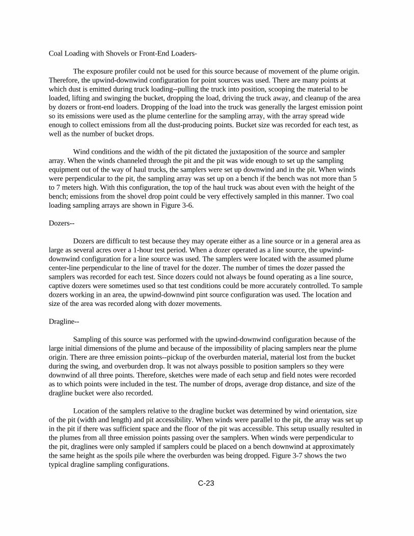
C-23
Coal Loading with Shovels or Front-End Loaders-
The exposure profiler could not be used for this source because of movement of the plume origin.Therefore, the upwind-downwind configuration for point sources was used. There are many points atwhich dust is emitted during truck loading--pulling the truck into position, scooping the material to beloaded, lifting and swinging the bucket, dropping the load, driving the truck away, and cleanup of the areaby dozers or front-end loaders. Dropping of the load into the truck was generally the largest emission pointso its emissions were used as the plume centerline for the sampling array, with the array spread wideenough to collect emissions from all the dust-producing points. Bucket size was recorded for each test, aswell as the number of bucket drops.
Wind conditions and the width of the pit dictated the juxtaposition of the source and samplerarray. When the winds channeled through the pit and the pit was wide enough to set up the samplingequipment out of the way of haul trucks, the samplers were set up downwind and in the pit. When windswere perpendicular to the pit, the sampling array was set up on a bench if the bench was not more than 5to 7 meters high. With this configuration, the top of the haul truck was about even with the height of thebench; emissions from the shovel drop point could be very effectively sampled in this manner. Two coalloading sampling arrays are shown in Figure 3-6.
Dozers--
Dozers are difficult to test because they may operate either as a line source or in a general area aslarge as several acres over a 1-hour test period. When a dozer operated as a line source, the upwind-downwind configuration for a line source was used. The samplers were located with the assumed plumecenter-line perpendicular to the line of travel for the dozer. The number of times the dozer passed thesamplers was recorded for each test. Since dozers could not always be found operating as a line source,captive dozers were sometimes used so that test conditions could be more accurately controlled. To sampledozers working in an area, the upwind-downwind pint source configuration was used. The location andsize of the area was recorded along with dozer movements.
Dragline--
Sampling of this source was performed with the upwind-downwind configuration because of thelarge initial dimensions of the plume and because of the impossibility of placing samplers near the plumeorigin. There are three emission points--pickup of the overburden material, material lost from the bucketduring the swing, and overburden drop. It was not always possible to position samplers so they weredownwind of all three points. Therefore, sketches were made of each setup and field notes were recordedas to which points were included in the test. The number of drops, average drop distance, and size of thedragline bucket were also recorded.
Location of the samplers relative to the dragline bucket was determined by wind orientation, sizeof the pit (width and length) and pit accessibility. When winds were parallel to the pit, the array was set upin the pit if there was sufficient space and the floor of the pit was accessible. This setup usually resulted inthe plumes from all three emission points passing over the samplers. When winds were perpendicular tothe pit, draglines were only sampled if samplers could be placed on a bench downwind at approximatelythe same height as the spoils pile where the overburden was being dropped. Figure 3-7 shows the twotypical dragline sampling configurations.

C-24
Sampling array on a bench
Figure 3-6. Coal loading with upwind-downwind configuration.
Sampling array in the pit

C-25
Sampling array in the pit
Sampling array at about the same height as the spoils pile
Figure 3-7. Dragline sampling with upwind-downwind concentration.
C-26
Haul Trucks--
Most sampling periods for haul trucks at the first mine were performed as part of thecomparability study (see Section 6), employing both exposure profiling and upwind-downwind configura-tions. Haul trucks were used to perform the comparative study because they are a uniformly-emitting linesource and because haul road traffic is the largest particulate source in most mines. At subsequent mines,exposure profiling was used to sample this source. For each test, the wind was approximatelyperpendicular to the road, the air intakes of the samplers were pointed directly into the wind, and thesamplers extended to a height of 6 m to capture the vertical extent of the plume. In a few cases, more than<U10 of the plume mass extended above the top sampler because of a combination of light winds, unstableatmospheric conditions, and large vehicles. Consistent travel speed and diversion of watering trucks wasrequested during each sampling period. A haul truck sampling array in shown in Figure 3-8.
Light- and Medium-Duty Vehicles--
The sampling methodology for this category of vehicles was nearly identical to the haul truckprocedures. The only exceptions were that: (l) a 4 m sampler height was adequate to sample the plumefrom the smaller vehicles and (2) pickup trucks belonging to the contractor were used for better control ofvehicle speed and weight. In most cases, access roads specifically for lighter vehicles were used for testing.However, some sampling for light- and medium-duty vehicles was done on haul roads. Samples of the roadsurfaces were taken so that differences due to road properties could be evaluated (a full discussion ofsource characterization is included in the next subsection). A light- and medium-duty vehicle samplingarray is shown in previously cited Figure 3-8.
Scraper--
This source was sampled by the exposure profiling method. Scrapers were sampled while travelingon a temporary road so that the emissions could be tested as a line source. Neither the loading nor theemptying operations were sampled, since both had been estimated to have insignificant emissionscompared to scraper travel. The profiler was extended to 6 m to sample the vertical extent of the plume. Inorder to secure a suitable setup in a location without interference from other sources, it was oftennecessary to use captive equipment. A typical sampling array for scrapers IS shown in Figure 3-9.
Graders--
Exposure profiling was used to sample graders. Graders operate in a fairly constant manner; onlythe speed and travel surface (on road/off road) vary over time. It was assumed that the travel surface couldbe considered as a correction factor rather than requiring two separate emission factors. As with dozers,captive equipment was sometimes necessary to sample this source because graders did not normally drivepast the same location repetitively. Even if they were regrading a short stretch of road, they would be at adifferent location on the road cross section with each pass, making it difficult to reposition the profiler.Therefore, captive equipment allowed better control of test variables.

C-27
Haul truck level
Light- and medium-duty truck
Figure 3-8. Haul road sampling with exposure profiling configuration.

C-28
Figure 3-9. Scraper sampling with exposure profiling configuration.
C-29
Wind Erosion of Exposed Areas and Storage Piles--
The wind tunnel was used to sample these two sources. In measuring emissions with the portablewind tunnel, it was necessary to place the tunnel on a flat, nearly horizontal section of surface. Care wastaken not to disturb the natural crust on the surface, with the exception of removing a few large clumpsthat prevented the tunnel test section from making an airtight seal with the surface.
The threshold velocity for wind erosion and emission rates at several predetermined wind speedsabove the threshold were measured on each test surface. Wind erosion of exposed surfaces had been shownto decay in time for velocities well above the threshold value for the exposed surface. Therefore, some testsof a given surface were performed sequentially to trace the decay of the erosion rate over time at high testvelocities. A typical wind tunnel sampling configuration is shown in Figure 3-10.
Changes Made in Response to Comments
The basic sampling designs presented above represent the combined efforts of the two contractorsas well as comments received from the technical review group. Specific changes made in response totechnical review group comments are summarized below.
1. Dichotomous samplers were added to the exposure profiling sampling method. They wereplaced at four heights corresponding to the isokinetic sampling heights during thecomparability study, and at two heights for the remainder of the tests. With this arrangement,dichotomous samplers replaced the cascade impactor as the primary particle size sampler inexposure profiling.
2. A fourth row of downwind samplers was added to the upwind-downwind array. Two hi-volewere placed at 200 m from the source to aid in the measurement of deposition.
3. The quasi-stack sampling method was adopted for sampling overburden drilling and anenclosure was designed and fabricated.
4. The modification of the exposure profiling method to sample blasts was devised.
5. Provisions were made to sample scrapers, and other sources as required, as captive equipmentin locations not subject to other dust interferences.
SOURCE CHARACTERIZATION PROCEDURES
In order to determine the parameters that affect dust generation from an individual source, thesuspected parameters must be measured at the time of the emission test. These parameters fall into threecategories: properties of the materials being disturbed by wind or machinery, operating parameters of themining equipment involved, and meteorological conditions. Table 3-5 lists the potential parameters bysource that were quantified during the study.

C-30
Figure 3-10. Wind erosion sampling with wind tunnel.

C-31
TABLE 3-5. SOURCE CHARACTERIZATION PARAMETERS MONITORED DURING TESTING
Source Parametera Quantification Technique
All tests Wind speed and directionTemperatureSolar intensityHumidityAtmospheric pressurePercent cloud cover
AnemometerThermometerPyranographSling psychrometerBarometerVisual estimate
Overburden drilling Silt contentMoisture contentDepth of hole
Dry sievingOven dryingDrill operator
Blasting Number of holesSize of blast areaMoisture content
Visual countMeasurementFrom mining company
Coal loading Silt contentMoisture contentBucket capacityEquipment operation
Dry sievingOven dryingEquipment specificationsRecord variations
Dozer Silt contentMoisture contentSpeedBlade size
Dry sievingOven dryingTime/distanceEquipment specifications
Dragline Silt contentMoisture contentBucket capacityDrop distance
Dry sievingOven dryingEquipment specificationsVisual estimate
Haul truck Surface silt contentVehicle speedVehicle weightSurface loadingSurface moisture contentNumber of wheels
Dry sievingRadar gunTruck scaleMass/area of collected road sampleOven dryingVisual observation
Light- and medium-dutyvehicles
Same parameters and quantification techniques as for haul trucks
Scraper Same parameters and quantification techniques as for haul trucks
Grader Same parameters and quantification techniques as for haul trucks
Wind erosion of exposed areas Surface erodibilitySurface silt contentSurface moisture contentSurface roughness height
Dry sievingDry sieving, before and after testOven drying, before and after testMeasurement
Wind erosion of storage piles Same parameters and quantification techniques as for wind erosion of exposed areas
a Most of the meteorological parameters monitored during all tests are needed to estimate emission rates, and arenot considered to be potential correction parameters in the emission factor equations.

C-32
Representative samples of materials (topsoil, overburden, coal, or road surface) were obtained ateach test location. Unpaved and paved roads were sampled by removing loose material (by means ofvacuuming and/or broom sweeping) from lateral strips of road surface extending across the travel portion.Loose aggregate materials being transferred were sampled with a shovel to a depth exceeding the size ofthe largest aggregate pieces. Erodible surfaces were sampled to a depth of about 1 centimeter. The sampleswere analyzed to determine moisture and silt content.
Mining equipment travel speeds were measured by radar gun or with a stop watch over a knowntravel distance. Equipment specifications and traveling weights were obtained from mine personnel. Forseveral sources, it was necessary to count vehicle passes, bucket drops, etc. These counts were usuallyrecorded by two people during the test to ensure the accuracy of the results. Frequent photographs weretaken during each test to establish the sampling layout (to supplement the ground-measured distances),source activity patterns, and plume characteristics.
Micro-meteorological conditions were recorded for each test. Most of these data were used in thecalculation of concentrations or emission rates rather than as potential correction factors for the emissionfactor equations. During the test, a recording wind instrument measured wind direction and wind speed atthe sampling site. A pyranograph was used to measure solar intensity. Humidity was determined with asling psychrometer. A barometer was used to record atmospheric pressure. The percent of cloud cover wasvisually estimated.
In addition to monitoring micro-meteorological conditions, a fixed monitoring station at the minemonitored parameters affecting the entire area. Data were recorded on temperature, humidity, wind speedand direction, and precipitation.
ADJUSTMENTS MADE DURING SAMPLING
The sampling configurations detailed in this section were the result of a careful study designprocess completed prior to actual field sampling. Actual field conditions forced changes to elements of thestudy design.
A modification to the upwind-downwind sampling array was required. Whereas the study designcalled for two hi-vole at 200 m downwind of the source, this setup could not be adapted to field conditions.Three major reasons for the deviation from the study designs were: (a) the difficulty of locating thesamplers where they were not subjected to other dust interferences; (b) the difficulty of extending power tothe samplers; and © in many sampling locations, there was not 200 m of accessible ground downwind ofthe source. Therefore, only 1 hi-vol was routinely placed at the 200 m distance and in some cases nosampler was located at that distance.
Four modifications were made to the exposure profiling sampling array. First, it was impracticalto mount dichotomous samplers at all four heights on the profiling tower as called for in the original studydesign. Dichotomous samplers were placed at two heights. Second, the study design called for an exposureprofiling test to be terminated if the standard deviation of the wind direction exceeded 22.5° during the testperiod. Because unstable atmospheric conditions were encountered at Mine 1 during the summer season, itwas necessary to relax this restriction. However, this change had no effect on the direction-insensitivedichotomous sampler which served as the primary sizing device. At the third mine, a second cascadeimpactor and hi-vol were added alongside the profiler at the height of the third profiling head. This was to
C-33
provide backup data on particle size distribution in the upper portion of the plume and on the TSPconcentration profile. Finally, greased substrates were used with the cascade impactors at the third mine totest whether particle bounce-through observed at the first two mines would be diminished.
A modification was required to the balloon sampling array. The study design specified that thefive ground-based sampler pairs be located 10 m apart and that the balloon samplers be located on theblast plume centerline. This was found to be impractical under field conditions. The location of the plumecenterline was very dependent on the exact wind direction at the time of the blast. Because the balloonsampling array required at least one hour to set up, it was impossible to anticipate the exact wind directionone hour hence. Therefore, the ground-based samplers were placed 20 to 30 m apart when the wind wasvariable so that some of the samplers were in the plume. The balloon sometimes could not be moved to theplume centerline quickly enough after the blast. Rapid sequence photography was used during the test toassist in determining the plume centerline) the emission factor calculation procedure was adjustedaccordingly.
ERROR ANALYSES FOR SAMPLING METHODS
Separate error analyses were prepared for the exposure profiling and upwind-downwind samplingmethods. These analyses were documented in interim technical reports and will only be summarized here(Midwest Research Institute 1979; PEDCo Environmental 1979).
A summary of potential errors (lF) in the exposure profiling method initially estimated by MRI isshown in Table 3-6. Potential errors fall in the categories of sample collection, laboratory analysis, andemission factor calculation. For particles less than 15 Fm, the error in the technique was estimated byMRI to range from -14 percent to +8 percent. Subsequent field experience on this project indicated thatactual error was 30 to 35 percent in that size range and higher for the less than 30 Fm (suspendedparticulate) size range.
Potential errors initially estimated by PEDCo for the upwind-downwind sampling method aresummarized in Table 3-7. A delineation was made between errors associated with line sources andpoint/area sources. The estimated errors were ±30.5 percent and ±50.1 percent, respectively.
SUMMARY OF TESTS PERFORMED
Sampling performed is shown in Table 3-8. The number of samples are shown by source andmine. A total of 265 tests were completed.
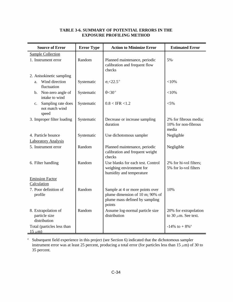
C-34
TABLE 3-6. SUMMARY OF POTENTIAL ERRORS IN THEEXPOSURE PROFILING METHOD
Source of Error Error Type Action to Minimize Error Estimated Error
Sample Collection1. Instrument error Random Planned maintenance, periodic
calibration and frequent flowchecks
5%a
2. Anisokinetic samplinga. Wind direction
fluctuationSystematic F2<22.5E <10%
b. Non-zero angle ofintake to wind
Systematic 2<30E <10%
c. Sampling rate doesnot match windspeed
Systematic 0.8 < IFR <1.2 <5%
3. Improper filter loading Systematic Decrease or increase samplingduration
2% for fibrous media;10% for non-fibrousmedia
4. Particle bounce Systematic Use dichotomous sampler NegligibleLaboratory Analysis5. Instrument error Random Planned maintenance, periodic
calibration and frequent weightchecks
Negligible
6. Filter handling Random Use blanks for each test. Controlweighing environment forhumidity and temperature
2% for hi-vol filters;5% for lo-vol filters
Emission FactorCalculation7. Poor definition of
profileRandom Sample at 4 or more points over
plume dimension of 10 m; 90% ofplume mass defined by samplingpoints
10%
8. Extrapolation ofparticle sizedistribution
Random Assume log-normal particle sizedistribution
20% for extrapolationto 30 Fm. See text.
Total (particles less than15 Fm)
-14% to + 8%a
a Subsequent field experience in this project (see Section 6) indicated that the dichotomous samplerinstrument error was at least 25 percent, producing a total error (for particles less than 15 Fm) of 30 to35 percent.

C-35
TABLE 3-7. SUMMARY OF POTENTIAL ERRORS IN THEUPWIND-DOWNWIND SAMPLING METHOD
Estimated Error
Source of ErrorData Restraints to
Limit Error Line Source Point/Area Source
Measurement
1. High volume samplermeasurements
Orientation of roof withinaverage wind direction
18.8% 18.8%
2. Wind speed measurement Average wind speed >1.0mph
4.6% 4.6%
3. Location relative to thesource
a. Distance from source Measure from downwindedge of source
1.7% 1.7%
b. Distance from plumeé in y dimension
Samplers should be within2Fy of centerline
- 5.8E
c. Distance from plumeé in z dimension
Samplers should be within2Fz of centerline
0.5 m 1.0 m
Atmospheric DispersionEquation
4. Initial plume dispersionHorizontalVertical
-0.2 m
0.2 m0.5 m
5. Dispersion coefficientsEmpirical valuesEstimation of stabilityclass
3.2%15.9%
5.8/3.2%21.1/15.9%
6. Subtraction of abackground concentration
This error will be higherwhen the wind reversesbriefly or upwind samplersare biased by nearbysources
18.8% 18.8%
7. Gaussian plume shape cannot quantify
8. Steady state dispersion Marginal passes <12% ofgood passes
6.0% 6.0%
Total 30.5% 50.1%
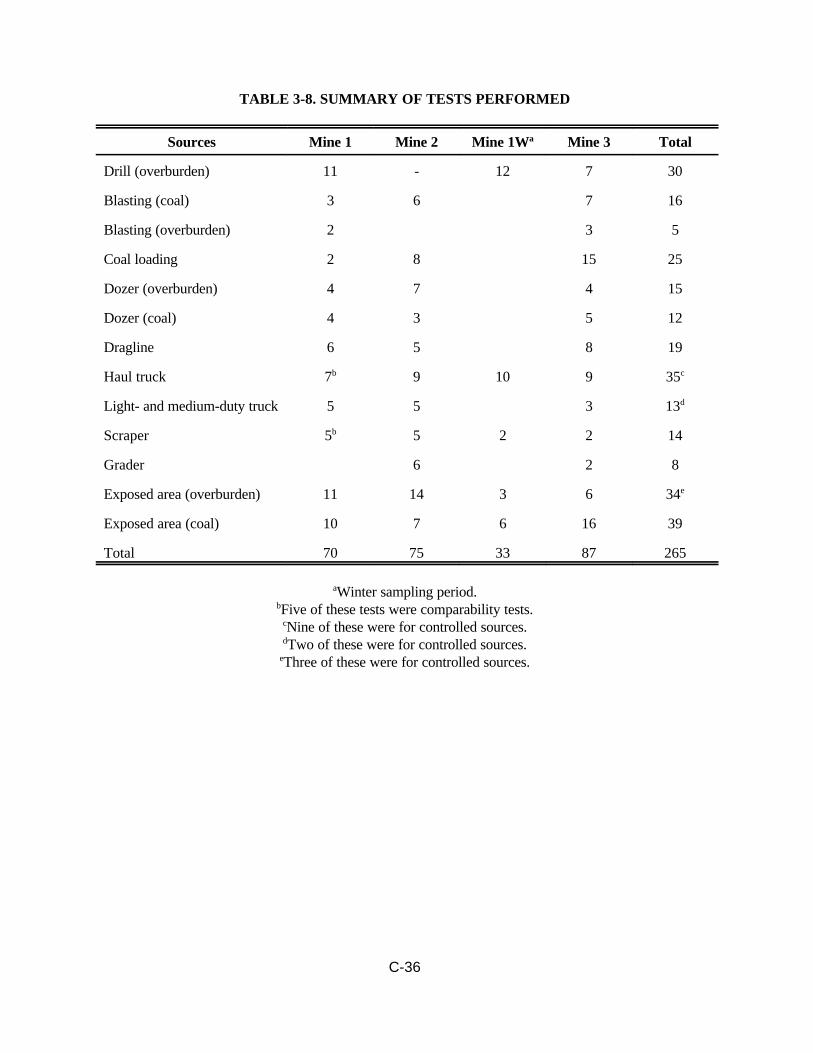
C-36
TABLE 3-8. SUMMARY OF TESTS PERFORMED
Sources Mine 1 Mine 2 Mine 1Wa Mine 3 Total
Drill (overburden) 11 - 12 7 30
Blasting (coal) 3 6 7 16
Blasting (overburden) 2 3 5
Coal loading 2 8 15 25
Dozer (overburden) 4 7 4 15
Dozer (coal) 4 3 5 12
Dragline 6 5 8 19
Haul truck 7b 9 10 9 35c
Light- and medium-duty truck 5 5 3 13d
Scraper 5b 5 2 2 14
Grader 6 2 8
Exposed area (overburden) 11 14 3 6 34e
Exposed area (coal) 10 7 6 16 39
Total 70 75 33 87 265
aWinter sampling period.bFive of these tests were comparability tests.
cNine of these were for controlled sources.dTwo of these were for controlled sources.
eThree of these were for controlled sources.

D-1
Appendix DSample Handling and Analysis
This appendix contains information on the handling and analysis of fugitive dust emission samples.
All information found in this appendix, is from section 4 of the EPA report “Improved Emission Factors
For Fugitive Dust From Western Surface Coal Mining Sources - Volume I -Sampling Methodology and
Test Results.”

D-2
TABLE OF CONTENTS
Page
D.1 Section 4 of Report: "Improved Emission Factors for Fugitive Dust From Western Surface Coal Mining Sources--Volume 1 - Sampling Methodology and Test Results . . . . . . . . . . . . . . . . . . . . . . . . . . . . . . . . . . . . . . . . . . . . . . . . . . . . . . . D-3

D-3
D.1 Section 4 of Report: "Improved Emission Factors for Fugitive Dust From Western Surface Coal
Mining Sources--Volume 1 - Sampling Methodology and Test Results.
SECTION 4
SAMPLE HANDLING AND ANALYSIS
SAMPLE HANDLING
Several different types of particulate samples were collected during the field work: hi-vol glass
filters, filters and settling chamber catches from exposure profilers, cascade impactor stages, cyclone
precollector catches, Teflon filters from dichotomous samplers, millipore filter cartridges for microscopic
analysis, PVC filters from the balloon sampling system, and dustfall samples. These samples all required
slightly different handling procedures.
At the end of each run, the collected samples were transferred carefully to protective containers.
All transfer operations except removal of cartridges from the instruments were done in a van or in the field
lab to minimize sample losses and contamination. Sample media were carried and transported locally in an
upright position, and covered with temporary snap-on shields or covers where appropriate. Hi-vol and
profiler filters were folded and placed in individual envelopes. Dust collected on interior surfaces of profiler
probes and cyclone precollectors was rinsed with distilled water into containers with the settling chamber
catches.
In order to reduce the amount of material dislodged from the taut dichotomous filters during
handling, the preweighed filters were placed in plastic holders that were then kept in individual petri dishes
throughout the handling process. The petri dishes were sealed with tape before being returned to the
laboratory and stacked in small carrying cases so that they would not be inverted. Many of the dichotomous
filters were hand-carried back to the laboratory by air travel rather than returning with the sampling
equipment and other samples in the van.
In spite of the special handling procedures adopted for the dichotomous filters, loose particulate
material was observed in some of the petri dishes and material could be seen migrating across the filter
surfaces with any bumping of the filter holder. Several corrective actions were investigated by PEDCo and

D-4
MRI throughout the study, but this remained an unresolved handling problem. First, ringed Teflon filters
were substituted for the mesh-backed filters initially used in an attempt to reduce movement or vibration of
the exposed filters. Next, the possibility of weighing the filters in the field was reviewed. However, a
sensitive microbalance and strict filter equilibration procedures were required because of the small weights
involved--filter tare weights less than 100 mg and many upwind and fine particle fraction sample weights
less than 50 Fg. (See Pages 12-4 and 12-5 for further discussion of dichotomous samplers.)
PVC filters for the balloon samplers and millipore filters for particle size analysis were sent to the
field in plastic cartridges. These cartridges were uncapped and affixed to the air pumps during sampling,
then resealed and returned to the laboratory for gravimetric or microscopic analysis. Loss of material from
these filter surfaces was not observed to be a problem as it was with the Teflon filters.
All samples except the dichotomous filters were labeled with the name of the mine, date, operation,
sampler, and a unique sample number (dichotomous sample holders had only the sample number). This
same information was also recorded on a field data sheet at the time of sampling. Copies of the field data
sheets were shown in the study design report.
To minimize the problem of particle bounce, the glass fiber cascade impactor substrates were
greased for use at Mine 3. The grease solution was prepared by dissolving 100 grams of stopcock grease in
1 liter of reagent grade toluene. A low pressure spray gun was used to apply this solution to the impaction
surfaces. No grease was applied to the borders and backs of the substrates. After treatment, the substrates
were equilibrated and weighed using standard procedures. The substrates were handled, transported and
stored in specially designed frames which protected the greased surfaces.
After samples were taken at the mines, they were kept in the field lab until returned to the main
laboratory. All samples were accounted for by the field crew by checking against the field data sheet
records prior to leaving the field location. Photocopies of the data sheets were made and transported sepa-
rately from the samples. Upon reaching the lab, the chain of custody was maintained by immediately
logging in the sample numbers of all samples received. No samples were known to have been lost through
misplacement or inadequate labeling during the entire study.
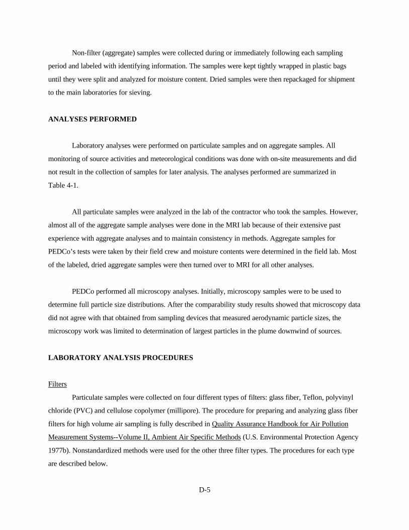
D-5
Non-filter (aggregate) samples were collected during or immediately following each sampling
period and labeled with identifying information. The samples were kept tightly wrapped in plastic bags
until they were split and analyzed for moisture content. Dried samples were then repackaged for shipment
to the main laboratories for sieving.
ANALYSES PERFORMED
Laboratory analyses were performed on particulate samples and on aggregate samples. All
monitoring of source activities and meteorological conditions was done with on-site measurements and did
not result in the collection of samples for later analysis. The analyses performed are summarized in
Table 4-1.
All particulate samples were analyzed in the lab of the contractor who took the samples. However,
almost all of the aggregate sample analyses were done in the MRI lab because of their extensive past
experience with aggregate analyses and to maintain consistency in methods. Aggregate samples for
PEDCo’s tests were taken by their field crew and moisture contents were determined in the field lab. Most
of the labeled, dried aggregate samples were then turned over to MRI for all other analyses.
PEDCo performed all microscopy analyses. Initially, microscopy samples were to be used to
determine full particle size distributions. After the comparability study results showed that microscopy data
did not agree with that obtained from sampling devices that measured aerodynamic particle sizes, the
microscopy work was limited to determination of largest particles in the plume downwind of sources.
LABORATORY ANALYSIS PROCEDURES
Filters
Particulate samples were collected on four different types of filters: glass fiber, Teflon, polyvinyl
chloride (PVC) and cellulose copolymer (millipore). The procedure for preparing and analyzing glass fiber
filters for high volume air sampling is fully described in Quality Assurance Handbook for Air Pollution
Measurement Systems--Volume II, Ambient Air Specific Methods (U.S. Environmental Protection Agency
1977b). Nonstandardized methods were used for the other three filter types. The procedures for each type
are described below.
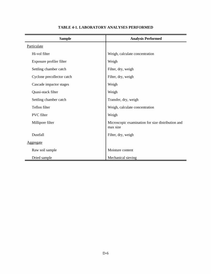
D-6
TABLE 4-1. LABORATORY ANALYSES PERFORMED
Sample Analysis Performed
Particulate
Hi-vol filter Weigh, calculate concentration
Exposure profiler filter Weigh
Settling chamber catch Filter, dry, weigh
Cyclone precollector catch Filter, dry, weigh
Cascade impactor stages Weigh
Quasi-stack filter Weigh
Settling chamber catch Transfer, dry, weigh
Teflon filter Weigh, calculate concentration
PVC filter Weigh
Millipore filter Microscopic examination for size distribution andmax size
Dustfall Filter, dry, weigh
Aggregate
Raw soil sample Moisture content
Dried sample Mechanical sieving
D-7
Glass fiber filters were numbered and examined for defects, then equilibrated for 24 hours at 70EF
and less than 50 percent relative humidity in a special weighing room. The filters were weighed to the
nearest 0.1 mg. The balance was checked at frequent intervals with standard weights to assure accuracy.
The filters remained in the same controlled environment for another 24 hours, after which a second analyst
reweighed 10 percent of them as a precision check. All the filters in each set in which check weights varied
by more than 3.0 mg from initial weights were reweighed. After weighing, the filters were packed flat,
alternating with onionskin paper, for shipment to the field.
When exposed filters were returned from the field, they were equilibrated under the same
conditions as the initial weighing. They were weighed and check weighed in the same manner.
Teflon filters from dichotomous samplers were desiccated for 24 hours over anhydrous calcium
sulfate (Drierite) before weighing, both before and after use. The filters were weighed in the same constant
temperature and humidity room as the glass fiber filters. They were weighed to the nearest 0.01 mg and the
check weighing had to agree within 0.10 mg or all filters in the set were reweighed. The filters themselves
were not numbered, but were placed in numbered petri dishes for handling and transport. Plastic filter
holders were also placed on the filters in the lab so they could be inserted directly into the dichotomous
samplers in the field.
PVC filters were treated in exactly the same manner as the Teflon filters, with the exception that
they were placed in plastic cartridges rather than petri dishes.
The millipore filters used for microscopic analysis were not weighed to determine the amount of
material collected. After they were exposed and returned to the lab in a plastic cartridge, a radial section of
the filter was cut and mounted on a glass microscope slide. The filter section was then immersed in an
organic fluid that rendered it invisible under the microscope, and a cover slip was placed over it. The slide
was examined under a light microscope at 100 power using phase contrast illumination. The particles were
sized by comparison with a calibrated reticle in the eyepiece. Ten different fields and at least 200 particles
were counted on each slide. Also, the diameters of the three largest individual particles observed were
recorded.
D-8
Settling Chamber Catches and Dustfall Samples
Laboratory grade dionized distilled water was used in the field laboratory to recover samples from
settling chambers and dustfall buckets. Each unit was thoroughly washed five to eight separate times. A
wash consisted of spraying 15 to 25 ml of water into the unit, swirling the unit around, and then quanti-
tatively pouring the water into a sample jar. After the last wash, the sample jar (holding 150 ± 50 ml of
wash water) was sealed and packed for shipping to MRI for sample recovery.
At the MRI laboratory, the entire wash solution was passed through a 47 mm Buchner type funnel
holding a Type AP glass fiber filter under suction. The sample jar was then rinsed twice with 10 to 20 ml
of dionized water. This water was passed through the Buchner funnel ensuring collection of all suspended
material on the 47 mm filter. The tared filter was then dried in an oven at 100°C for 24 hours. After drying,
the filters were conditioned at constant temperature 24 ± 2°C and constant humidity 45 ± 5 percent relative
humidity for 24 hours.
All filters, both tared and exposed, were weighed to ±5 Fg with a 10 percent audit of tared and
exposed filters. Audit limits were ±100 Fg. Blank values were determined by washing “clean” (unexposed)
settling chambers and dustfall buckets in the field and following the above procedures.
Aggregate Samples
Samples of road dust and other aggregate materials were collected in 20 to 25 kg quantities for
analysis of moisture and silt content. The samples were stored briefly in airtight plastic bags, then reduced
with a sample splitter (riffle) or by coning and quartering to about 1 kg (800 to 1600 g).
The final split samples were placed in a tared metal pan, weighed on a balance, and dried in an
oven at 110°C overnight. Laboratory procedures called for drying of materials composed of hydrated
minerals or organic materials like coal and certain soils for only 2 hours. The samples were then reweighed
and the moisture content calculated as the weight loss divided by the original weight of the sample alone.
This moisture analysis was done in the field lab.

D-9
Dried samples were placed in plastic containers and sealed for shipment to main laboratories for
determination of silt contents. This was done by mechanical dry sieving, with the portion passing a 200-
mesh screen constituting the silt portion. The nest of sieves was placed on a conventional sieve shaker for
15 min. The material passing the 200-mesh screen, particles of less than 75 Fm diameter, constituted the
smallest particles which could be accurately determined by dry sieving according to ASTM methods.
More detailed sample collection and laboratory procedures for the moisture and silt analyses were
presented in an appendix to the study design report.
QUALITY ASSURANCE PROCEDURES AND RESULTS
Quality assurance was an important concern from the beginning of this field study because of its
size, complexity, and importance. Several special activities were instituted as part of the overall quality
assurance effort. The primary one was delineation of specific quality assurance procedures to be followed
throughout the study. This list of procedures was subjected to review by the technical review group; a
revised version is presented in Table 4-2. It covers sampling flow rates, sampling media, sampling
equipment and data calculations.
In addition to the quantitative checks listed in Table 4-2, many nonquantifiable procedures related
to sample handling and visual inspection of equipment were adopted. Some of these were based on standard
practices but others were set more stringent than normal requirements. No quality assurance procedures for
operating or maintaining dichotomous samplers had been recommended yet by EPA, so considerable
project effort was expended in developing and testing these procedures.
Meteorological equipment and monitoring procedures are not covered in Table 4-2. Approved
equipment was used and it was operated and maintained according to manufacturer’s instructions.
Meteorological instruments had been calibrated in a laboratory wind tunnel prior to the field work.
Adherence to the specified quality assurance procedures was checked periodically by the Project
Officer and other members of the technical review group, by intercontractor checks, and by external
independent audits. Results of the quality assurance program for flow rates and weighing are summarized
in Table 4-3. Results of the audits are described in the following section.

D-10
TABLE 4-2. QUALITY ASSURANCE PROCEDURES FOR MINING EMISSIONFACTOR STUDY
Activity QA Check/Requirement
Sampling flow rates
Calibration
Profilers, hi-vols, andimpactors
Calibrate flows in operating ranges using calibration orifice, once at eachmine prior to testing.
Dichotomous samplers Calibrate flows in operating ranges with displaced volume test metersonce at each mine prior to testing.
Single-point checksProfilers, hi-vols, andimpactors
Check 25% of units with rotameter, calibration orifice, electroniccalibrator once at each site prior to testing (different units each time). Ifany flows deviate by more than 7%, check all other units of same typeand recalibrate non-complying units. (See alternative check below).
Dichotomous samplers Check 25% of units with calibration orifice once at each site prior totesting (different units each time). If any flows deviate by more than 5%,check all other units and recalibrate non-complying units.
Alternative If flows cannot be checked at test site, check all units every two weeksand recalibrate units which deviate by more than 7% (5% for dichots).
Orifice calibration Calibrate against displaced volume test meter annually.
Sampling media
Preparation Inspect and imprint glass fiber media with ID numbers.
Inspect and place Teflon media (dichot filters) in petri dishes labeled withID numbers.
Conditioning Equilibrate media for 24 hours in clean controlled room with relativehumidity of less than 50% (variation of less than ±5%) and withtemperature between 20°C and 25°C (variation of less than ±3%).
Weighing Weigh hi-vol filters and impactor substrates to nearest 0.1 mg and weighdichot filters to nearest 0.01 mg.
Auditing of weights (tareand final)
Independently verify weights of 7% of filters and substrates (at least 4from each batch). Reweigh batch if weights of any hi-vol filters orsubstrates deviate by more than ±3.0 mg or if weights of any dichotfilters deviate by more than ±0.1 mg.
Correction for handlingeffects
Weigh and handle at least one blank for each 10 filters or substrates ofeach type for each test.
Prevention of handlinglosses
Transport dichot filters upright in filter cassettes placed in protectivepetri dishes.
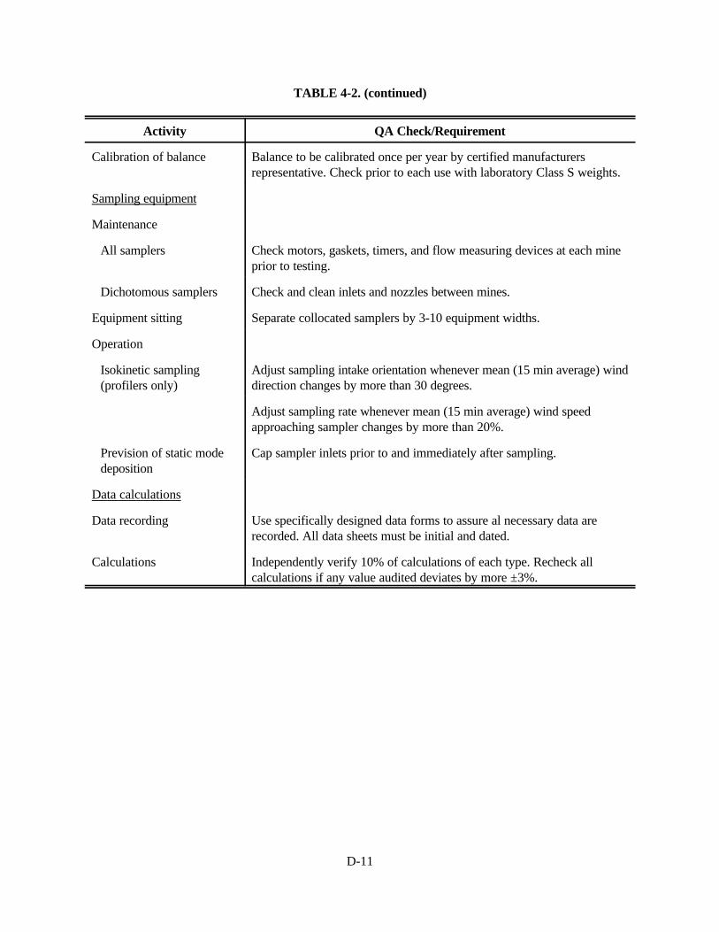
D-11
TABLE 4-2. (continued)
Activity QA Check/Requirement
Calibration of balance Balance to be calibrated once per year by certified manufacturersrepresentative. Check prior to each use with laboratory Class S weights.
Sampling equipment
Maintenance
All samplers Check motors, gaskets, timers, and flow measuring devices at each mineprior to testing.
Dichotomous samplers Check and clean inlets and nozzles between mines.
Equipment sitting Separate collocated samplers by 3-10 equipment widths.
Operation
Isokinetic sampling(profilers only)
Adjust sampling intake orientation whenever mean (15 min average) winddirection changes by more than 30 degrees.
Adjust sampling rate whenever mean (15 min average) wind speedapproaching sampler changes by more than 20%.
Prevision of static modedeposition
Cap sampler inlets prior to and immediately after sampling.
Data calculations
Data recording Use specifically designed data forms to assure al necessary data arerecorded. All data sheets must be initial and dated.
Calculations Independently verify 10% of calculations of each type. Recheck allcalculations if any value audited deviates by more ±3%.

D-12
TABLE 4-3. QUALITY ASSURANCE RESULTS
Activity QA Check/Requirement
Calibration
Profilers, hi-vols, andimpactors
PEDCo calibrated hi-vols a total of 6 times in the 4 visits.
MRI had flow controllers on all 3 types of units. These set flows werecalibrated a total of 4 times for profilers, 7 times for hi-vols andimpactors.
Dichotomous samplers PEDCo and MRI calibrated their 9 dichots a total of 6 times, at leastonce at each mine visit. Actual flow rates varied as much as 9.1%between calibrations.
Single point checks
Profilers, hi-vols, andimpactors
Out of a total of 29 single point checks, only 2 PEDCo hi-vols werefound to be outside the 7% allowable deviation, thus requiringrecalibration. For MRI, 20 single point checks produced no units out ofcompliance.
Dichotomous samplers The dichotomous samplers were recalibrated with a test meter each timerather than checking flow with a calibrated orifice.
Weighings
Tare and final weights PEDCo reweighed a total of 250 unexposed and exposed hi-vol filtersduring the study. Three of the reweighings differed by more than 3.0 mg.For 238 dichot filter reweighings, only four differed by more than 0.1mg.
MRI reweighed a total of 524 unexposed and exposed glass fiber filtersduring the study. Four of the reweighings differed by more than 3.0 mg.For 43 dichot filter reweighings, only one differed by more than 0.1 mg.
Blank filters PEDCo analyzed 88 blank hi-vol and 69 blank dichot filters. The averageweight increase was 3.4 mg (0.087%) for hi-vols, 0.036 mg (0.038%) fordichots. The highest blanks were 26.3 and 0.22 mg, respectively.
MRI analyzed 67 hi-vol and dichot filter blanks. The highest blanks were7.05 mg and 0.52 mg, respectively.
D-13
AUDITS
In addition to the rigorous internal quality assurance program and the review procedures set up
with the technical review group, several independent audits were carried out during this study to further
increase confidence in results. Two different levels of audits were employed:
Intercontractor - MRI audited PEDCo and vice versa
External - Performed by an EPA instrument or laboratory expert or a third EPA contractor
The audit activities and results of audits are summarized in Table 4-4.
Although there are no formal pass/fail criteria for audits such as these, all of the audits except the
collocated samplers in the comparability study and filter weighings seemed to indicate that measurements
were being made correctly and accurately. The collocated sampler results are discussed further in Sections
6 and 12. All the filters that exceeded allowable tolerances upon reweighing (10 percent of audited filters)
lost weight. In the case of the hi-vol filters, loose material was observed in the filter folders and noted on
the MRI data sheet. The amounts lost from the dichot filters would not be as readily noticeable in the petri
dishes. The several extra handling steps required for auditing the filters, including their transport from
Cincinnati to Kansas City, could have caused loss of material from the filters.
In addition to the external flow calibration audit at the third mine (shown in Table 4-4), another one
was conducted at the second mine. However, results of this earlier audit were withdrawn by the contractor
who performed it after it was learned that some critical steps, such as the auditee being present and current
calibration curves being provided at the time of the audit, had not been followed. However, the preliminary
results of that withdrawn audit showed generally acceptable performance of almost all the sampling
equipment.
Some of the calculations of each contractor were repeated by the other as an audit activity. In
general, the data were found to be free of calculation errors, but differences in assumptions and values read
from curves led to frequent differences in final emission rates. No effort was made to estimate the average
difference in independently calculated emission rates.

D-14
TABLE 4-4. AUDITS CONDUCTED AND RESULTS
Activity
Inter-Contractoror External
AuditContractor
Audited Date
No. andType ofUnits Results
Flow Calibration I PEDCo 8-22-79 2 hi-vol Each 4% from cal. curve
MRI 8-27-79 1 hi-vol1 impactor2 dichot
Hi-vol and impactor within 4%of curve; dichot within 2%
PEDCo 10-12-79 2 hi-vol One within 1%, other out by12.6%
MRI 10-12-79 2 hi-vol1 dichot
Both within 7%Within 5%
E(EPA,
OAQPS)
PEDCo 8-01-79 7 dichot All set 5 to 11% high
MRI 8-01-79 2 dichot One within 1%, other out by10%
E(contractor)
MRI 8-06-80
PEDCo 8-05-80 10 hi-vol 7 within 5%, 2 within 7%, one8.3% from cal. curve
PEDCo 8-06-80 5 dichot Total flows all within 5%, 2coarse flows differed by 6.2 and9.2%
Filter weighing I PEDCo 1-02-80 39 hi-vol31 dichot
Three hi-vol filters varied bymore than 5.0 mg; all lost weightand loose material in folder wasnoted. Four dichots exceededthe 0.10 mg tolerance and alllost weight
MRI - Filters not submitted yet
Laboratory procedures E(EPA,
EMSL)
PEDCo 10-30-79 Compreh.review
No problems found
MRI 11-13-79 Compreh.review
No problems found
Collocated samplers I Both 7-26-79 to8-09-79
18 hi-vol10 dichot
Paired hi-vol values differed byan avg. of 34%; IP values by35%
Systems audit E(EPA,
OAQPS)
Both 8-01-79 All Checked siting, calibration, filterhandling, and maintenanceprocedures. Few minorproblems found but concludedthat operations should providereliable data

E-1
Appendix E
Materials Related to Blasting Emission Factor
This appendix contains information related to emission factors for blasting. The information
contained in the appendix includes four items: Section 5.5 and 8.5 of “Fugitive Dust Emission Factor
Update for AP-42 ”; memorandum from Chatten Cowherd, MRI, to James Southerland, EPA, June 1986;
memorandum from Greg Muleski, MRI, to Frank Noonan, EPA, April 1987; and Section 9 of “Improved
Emission Factors For Fugitive Dust From Western Surface Coal Mining Sources--Volume I -Sampling
Methodology and Test Results.”

E-2
TABLE OF CONTENTS
Page
E.1 Section 5.5 and 8.5 of "Fugitive Dust Emission Factor Update for AP-42 . . . . . . . . . E-3
E.2 Memorandum from Chatten Cowherd, MRI, to James Southerland, EPA, June 1986 E-26
E.3 Memorandum from Greg Muleski, MRI, to Frank Noonan, EPA, April 1987 . . . . . . E-30
E.4 Section 9 of “Improved Emission Factors For Fugitive Dust From Western
Surface Coal Mining Sources--Volume I -Sampling Methodology and
Test Results.” . . . . . . . . . . . . . . . . . . . . . . . . . . . . . . . . . . . . . . . . . . . . . . . . . . . . . E-34

E-3
TABLE 23. COAL STORAGE SOURCE TESTING INFORMATION(Test Report 4)
Operation Equipment Material Site Test date No. of tests
Wind erosion Storage pile Coal Plant 1 3/74 2
8/74 2
E.1 Section 5.5 and 8.5 of "Fugitive Dust Emission Factor Update for AP-42
5.5 Section 8.24 - Western Surface Coal Mining and Processing
5.5.1 Test Report 4 (1977)
This study developed an emission factor for coal storage only. Four tests at one coal storage pile
(location not given) were conducted using the upwind-downwind technique. Table 23 presents the source
testing information fo r this study.
High-volume samplers were used to collect the airborne particulates from one upwind and four
downwind positions. The wind parameters were recorded at 15-min intervals. A sampling array similar to
that described in Section 5.3.2 (Test Report 6) was employed in this study. This sampling system meets the
minimum requirements of the upwind-downwind sampling technique. Optical microscopy was employed to
determine a particle size distribution. However, the particle size distribution for the emission factor was
determined from particle counting only (not-mass fraction), which is unrepresentative of a mass size
distribution.
This methodology is of generally sound quality; and emission rates were determined in a similar
manner to that described in Section 5.3.2 (Test Report 6). However, the report lacks sufficient detail for
adequate validation. For example, no indication is given as to sampling height. Also the field data recorded
at the sampling stations are not presented. The test data are therefore rated B.
Table 24 presents the developed emission factor, conditions tested and the appropriate rating. Only
one pile was sampled, although it was two different sizes during testing. The rating code refers to Table 4.
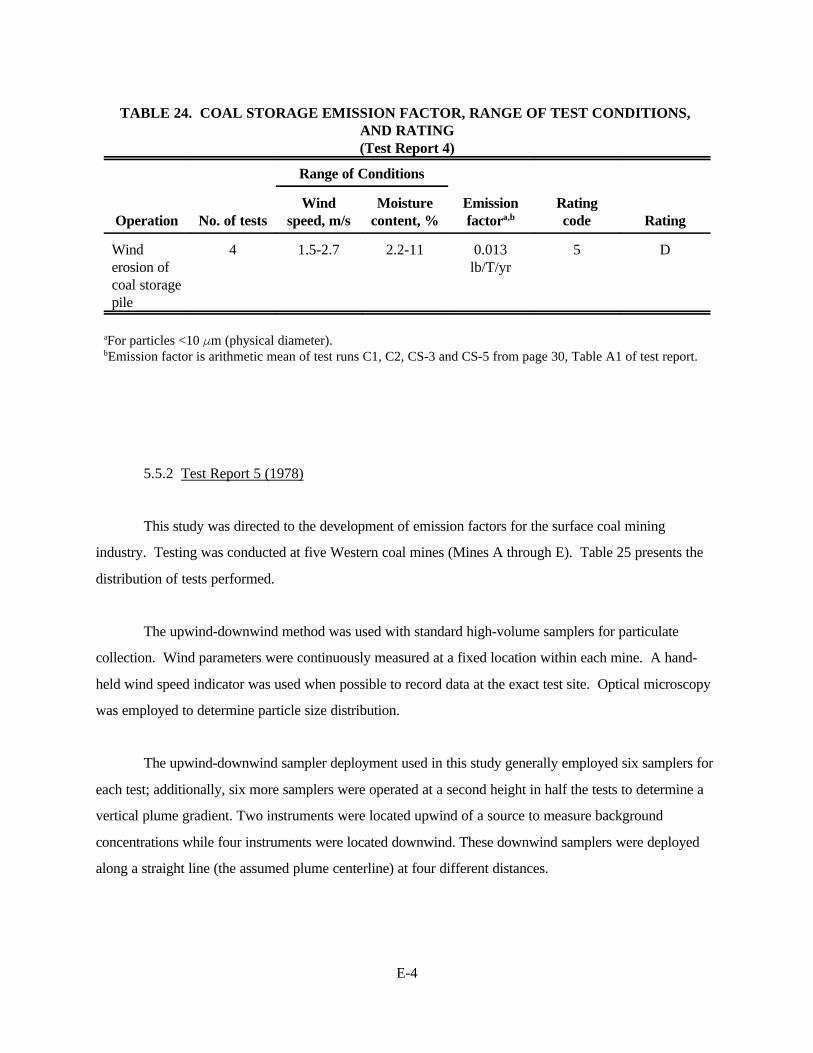
E-4
TABLE 24. COAL STORAGE EMISSION FACTOR, RANGE OF TEST CONDITIONS, AND RATING(Test Report 4)
Range of Conditions
Operation No. of testsWind
speed, m/sMoisture
content, %Emissionfactora,b
Ratingcode Rating
Winderosion ofcoal storagepile
4 1.5-2.7 2.2-11 0.013lb/T/yr
5 D
aFor particles <10 Fm (physical diameter).bEmission factor is arithmetic mean of test runs C1, C2, CS-3 and CS-5 from page 30, Table A1 of test report.
5.5.2 Test Report 5 (1978)
This study was directed to the development of emission factors for the surface coal mining
industry. Testing was conducted at five Western coal mines (Mines A through E). Table 25 presents the
distribution of tests performed.
The upwind-downwind method was used with standard high-volume samplers for particulate
collection. Wind parameters were continuously measured at a fixed location within each mine. A hand-
held wind speed indicator was used when possible to record data at the exact test site. Optical microscopy
was employed to determine particle size distribution.
The upwind-downwind sampler deployment used in this study generally employed six samplers for
each test; additionally, six more samplers were operated at a second height in half the tests to determine a
vertical plume gradient. Two instruments were located upwind of a source to measure background
concentrations while four instruments were located downwind. These downwind samplers were deployed
along a straight line (the assumed plume centerline) at four different distances.
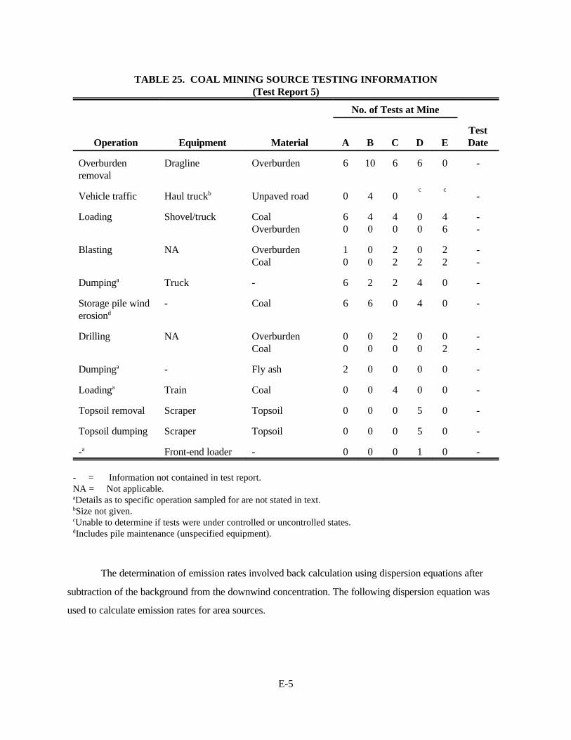
E-5
TABLE 25. COAL MINING SOURCE TESTING INFORMATION(Test Report 5)
No. of Tests at Mine
Operation Equipment Material A B C D ETestDate
Overburdenremoval
Dragline Overburden 6 10 6 6 0 -
Vehicle traffic Haul truckb Unpaved road 0 4 0c c
-
Loading Shovel/truck CoalOverburden
60
40
40
00
46
--
Blasting NA OverburdenCoal
10
00
22
02
22
--
Dumpinga Truck - 6 2 2 4 0 -
Storage pile winderosiond
- Coal 6 6 0 4 0 -
Drilling NA OverburdenCoal
00
00
20
00
02
--
Dumpinga - Fly ash 2 0 0 0 0 -
Loadinga Train Coal 0 0 4 0 0 -
Topsoil removal Scraper Topsoil 0 0 0 5 0 -
Topsoil dumping Scraper Topsoil 0 0 0 5 0 -
-a Front-end loader - 0 0 0 1 0 -
- = Information not contained in test report.NA = Not applicable.aDetails as to specific operation sampled for are not stated in text.bSize not given.cUnable to determine if tests were under controlled or uncontrolled states.dIncludes pile maintenance (unspecified equipment).
The determination of emission rates involved back calculation using dispersion equations after
subtraction of the background from the downwind concentration. The following dispersion equation was
used to calculate emission rates for area sources.
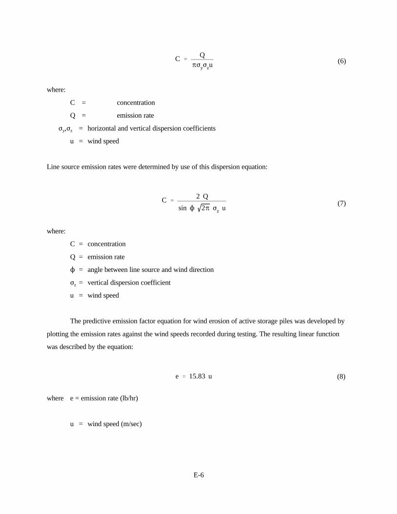
E-6
C 'Q
BFyFzu(6)
C '2 Q
sin N 2B Fz u(7)
e ' 15.83 u (8)
where:
C = concentration
Q = emission rate
Fy,Fz = horizontal and vertical dispersion coefficients
u = wind speed
Line source emission rates were determined by use of this dispersion equation:
where:
C = concentration
Q = emission rate
N = angle between line source and wind direction
Fz = vertical dispersion coefficient
u = wind speed
The predictive emission factor equation for wind erosion of active storage piles was developed by
plotting the emission rates against the wind speeds recorded during testing. The resulting linear function
was described by the equation:
where e = emission rate (lb/hr)
u = wind speed (m/sec)
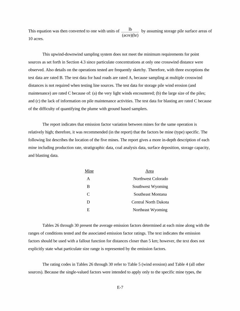
E-7
This equation was then converted to one with units of by assuming storage pile surface areas oflb(acre)(hr)
10 acres.
This upwind-downwind sampling system does not meet the minimum requirements for point
sources as set forth in Section 4.3 since particulate concentrations at only one crosswind distance were
observed. Also details on the operations tested are frequently sketchy. Therefore, with three exceptions the
test data are rated B. The test data for haul roads are rated A, because sampling at multiple crosswind
distances is not required when testing line sources. The test data for storage pile wind erosion (and
maintenance) are rated C because of: (a) the very light winds encountered; (b) the large size of the piles;
and (c) the lack of information on pile maintenance activities. The test data for blasting are rated C because
of the difficulty of quantifying the plume with ground based samplers.
The report indicates that emission factor variation between mines for the same operation is
relatively high; therefore, it was recommended (in the report) that the factors be mine (type) specific. The
following list describes the location of the five mines. The report gives a more in-depth description of each
mine including production rate, stratigraphic data, coal analysis data, surface deposition, storage capacity,
and blasting data.
Mine Area
A Northwest Colorado
B Southwest Wyoming
C Southeast Montana
D Central North Dakota
E Northeast Wyoming
Tables 26 through 30 present the average emission factors determined at each mine along with the
ranges of conditions tested and the associated emission factor ratings. The text indicates the emission
factors should be used with a fallout function for distances closer than 5 km; however, the text does not
explicitly state what particulate size range is represented by the emission factors.
The rating codes in Tables 26 through 30 refer to Table 5 (wind erosion) and Table 4 (all other
sources). Because the single-valued factors were intended to apply only to the specific mine types, the

E-8
requirement for more than one test site was waived. The rating for the equation developed for storage pile
wind erosion (and maintenance) is applicable when the equation is applied to mine types A, B, or D.
5.5.3 Test Report 14 (1981)
This study was conducted to determine improved fugitive dust emission factors for Western
surface coal mines. Field testing was conducted in three coal fields; Powder River Basin (Mine 1), North
Dakota (Mine 2), and Four Corners (Mine 3). The testing was performed during 1979 and 1980. Table 31
lists the testing information for this study.
The primary sampling method was exposure profiling. When source configuration made it
necessary, alternate methods were used, including upwind-downwind, balloon, and quasi-stack sampling.
Particle size distributions were determined by use of dichotomous samplers. Other equipment utilized were:
(a) high volume samplers for determining upwind concentrations; (b) dustfall buckets for determining
downwind particulate deposition; and (c) recording wind instruments to determine mean wind speed and
direction for adjusting the exposure profiler to isokinetic sampling conditions and for use in upwind-
downwind calculations.
Exposure profiling was used to measure emissions from moving point sources (see Table 31). The
exposure profiling sampling system was similar to that described in Section 5.1.1 and therefore meets the
minimum system design requirements. The upwind-downwind sampling system consisted generally of 15
particulate collection devices; 5 dichotomous samplers and 10 Hi-Vols.
One Hi-Vol and one dichotomous sampler were placed upwind while the remaining instruments
were placed at multiple downwind and crosswind distances. This system also meets the minimum upwind-
downwind requirements as described in Section 4.3.
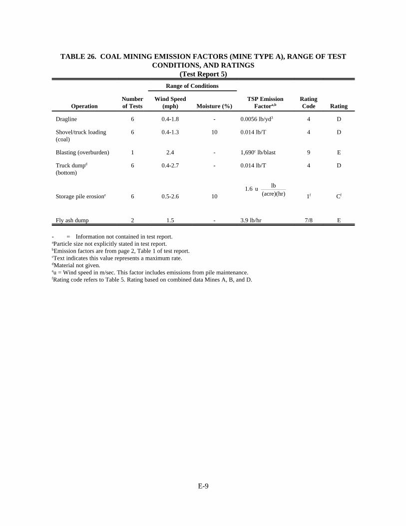
E-9
1.6 u lb(acre)(hr)
TABLE 26. COAL MINING EMISSION FACTORS (MINE TYPE A), RANGE OF TESTCONDITIONS, AND RATINGS
(Test Report 5)
Range of Conditions
OperationNumberof Tests
Wind Speed(mph) Moisture (%)
TSP EmissionFactora,b
RatingCode Rating
Dragline 6 0.4-1.8 - 0.0056 lb/yd3 4 D
Shovel/truck loading(coal)
6 0.4-1.3 10 0.014 lb/T 4 D
Blasting (overburden) 1 2.4 - 1,690c lb/blast 9 E
Truck dumpd
(bottom)6 0.4-2.7 - 0.014 lb/T 4 D
Storage pile erosione 6 0.5-2.6 10 1f Cf
Fly ash dump 2 1.5 - 3.9 lb/hr 7/8 E
- = Information not contained in test report.aParticle size not explicitly stated in test report.bEmission factors are from page 2, Table 1 of test report.cText indicates this value represents a maximum rate.dMaterial not given.eu = Wind speed in m/sec. This factor includes emissions from pile maintenance.fRating code refers to Table 5. Rating based on combined data Mines A, B, and D.
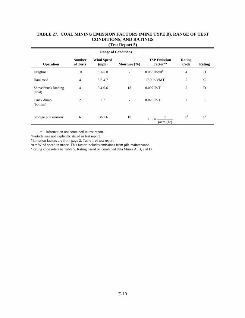
E-10
1.6 u lb(acre)(hr)
TABLE 27. COAL MINING EMISSION FACTORS (MINE TYPE B), RANGE OF TESTCONDITIONS, AND RATINGS
(Test Report 5)
Range of Conditions
OperationNumberof Tests
Wind Speed(mph) Moisture (%)
TSP EmissionFactora,b
RatingCode Rating
Dragline 10 3.1-5.8 - 0.053 lb/yd3 4 D
Haul road 4 3.7-4.7 - 17.0 lb/VMT 5 C
Shovel/truck loading(coal)
4 0.4-0.6 18 0.007 lb/T 5 D
Truck dump(bottom)
2 3.7 - 0.020 lb/T 7 E
Storage pile erosionc 6 0.8-7.6 18 1d Cd
- = Information not contained in test report.aParticle size not explicitly stated in test report.bEmission factors are from page 2, Table 1 of test report.cu = Wind speed in m/sec. This factor includes emissions from pile maintenance.dRating code refers to Table 5. Rating based on combined data Mines A, B, and D.
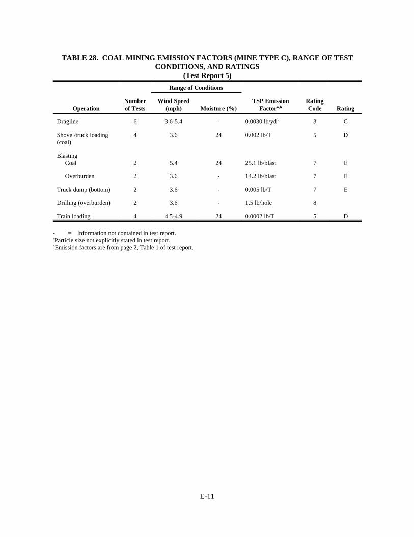
E-11
TABLE 28. COAL MINING EMISSION FACTORS (MINE TYPE C), RANGE OF TESTCONDITIONS, AND RATINGS
(Test Report 5)
Range of Conditions
OperationNumberof Tests
Wind Speed(mph) Moisture (%)
TSP EmissionFactora,b
RatingCode Rating
Dragline 6 3.6-5.4 - 0.0030 lb/yd3 3 C
Shovel/truck loading(coal)
4 3.6 24 0.002 lb/T 5 D
BlastingCoal 2 5.4 24 25.1 lb/blast 7 E
Overburden 2 3.6 - 14.2 lb/blast 7 E
Truck dump (bottom) 2 3.6 - 0.005 lb/T 7 E
Drilling (overburden) 2 3.6 - 1.5 lb/hole 8
Train loading 4 4.5-4.9 24 0.0002 lb/T 5 D
- = Information not contained in test report.aParticle size not explicitly stated in test report.bEmission factors are from page 2, Table 1 of test report.

E-12
1.6 u lb(acre)(hr)
TABLE 29. COAL MINING EMISSION FACTORS (MINE TYPE D), RANGE OF TESTCONDITIONS, AND RATINGS
(Test Report 5)
Range of Conditions
OperationNumberof Tests
Wind Speed(mph) Moisture (%)
TSP EmissionFactora,b
RatingCode Rating
Dragline 6 5.8-7.2 - 0.021 lb/yd3 3 C
Blasting (coal) 2 4.0 38 78.1 lb/blast 7 E
Truck dump (bottom) 4 4.5-6.7 - 0.027 lb/T 6 E
Storage pile erosionc 4 0.9-1.3 38 1d Cd
Topsoil removalScraping 5 5.8-7.6 - 0.35 lb/yd3 4 D
Dumping 5 2.2-3.6 - 0.03 lb/yd3 3 C
Front-end loader 1 2.7 - 0.12 lb/T 9 E
- = Information not contained in test report.aParticle size not explicitly stated in test report.bEmission factors are from page 2, Table 1 of test report.cu = Wind speed in m/sec.dRating code refers to Table 5. Rating based on combined data Mines A, B, and D.
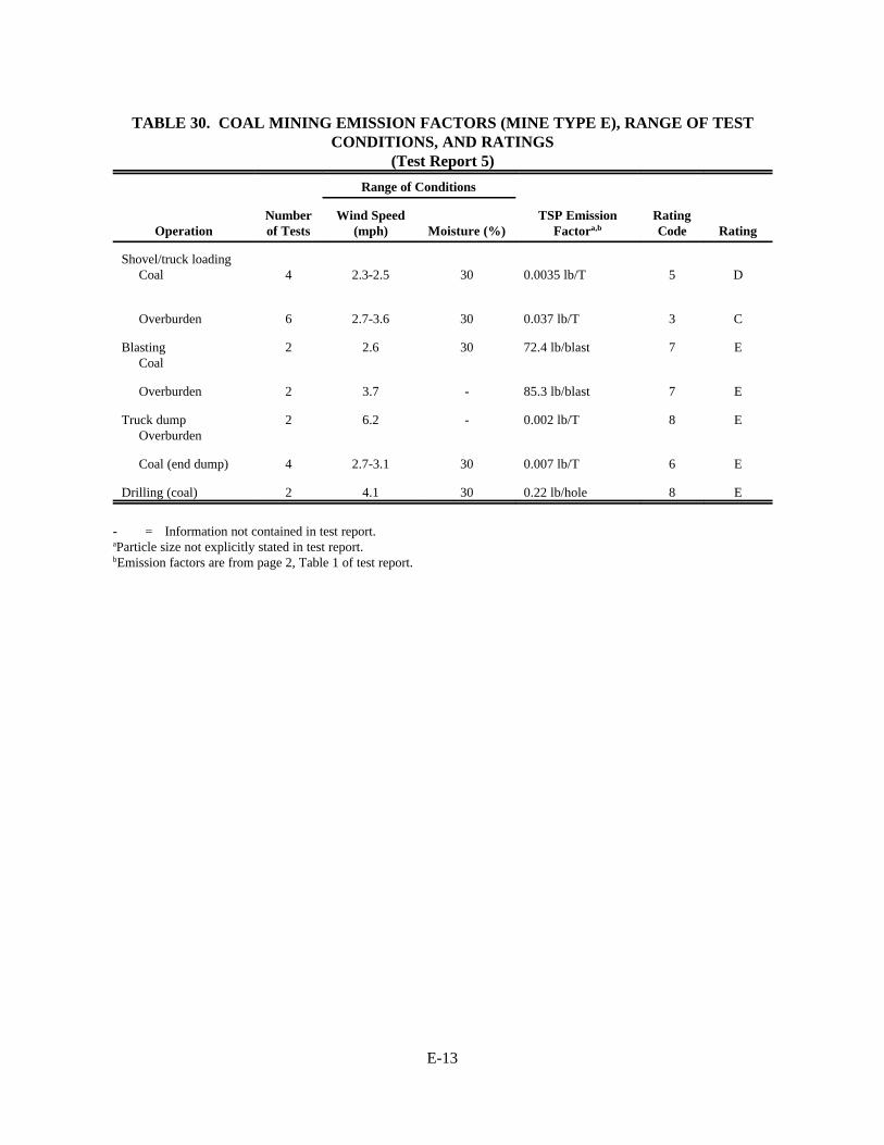
E-13
TABLE 30. COAL MINING EMISSION FACTORS (MINE TYPE E), RANGE OF TESTCONDITIONS, AND RATINGS
(Test Report 5)
Range of Conditions
OperationNumberof Tests
Wind Speed(mph) Moisture (%)
TSP EmissionFactora,b
RatingCode Rating
Shovel/truck loadingCoal 4 2.3-2.5 30 0.0035 lb/T 5 D
Overburden 6 2.7-3.6 30 0.037 lb/T 3 C
BlastingCoal
2 2.6 30 72.4 lb/blast 7 E
Overburden 2 3.7 - 85.3 lb/blast 7 E
Truck dumpOverburden
2 6.2 - 0.002 lb/T 8 E
Coal (end dump) 4 2.7-3.1 30 0.007 lb/T 6 E
Drilling (coal) 2 4.1 30 0.22 lb/hole 8 E
- = Information not contained in test report.aParticle size not explicitly stated in test report.bEmission factors are from page 2, Table 1 of test report.

E-14
TABLE 31. COAL MINING SOURCE TESTING INFORMATION (Test Report 14)
Operation Equipment Material Test Methoda Site (mine) Test Dates
No.of
Tests
Drilling NA Overburden Quasi-stack 1, 3 7/79, 8/79,12/79, 7/80
30
Blasting NA Coal Balloonb 1, 2, 3 8/79,10/79,7/80, 8/80
14
Overburden Balloonb 1, 3 8/79, 8/80 4
Loading Shovel/truck Coal Uw-Dw 1, 2 8/79, 10/79 10
Front-endloader/truck
Coal Uw-Dw 3 7/80, 8/80 15
Dozing Dozer Coal Uw-Dw 1, 2, 3 8/79,10/79, 8/80
12
Overburden Uw-Dw 1, 2, 3 8/79,10/79,7/80, 8/80
15
Dragline Dragline Overburden Uw-Dw 1, 2, 3 8/79,10/79,7/80, 8/80
19
Vehicle traffic Haul truck Unpaved road Uw-Dw 1 8/79, 12/79 11
Unpaved road Profiling 1, 2 ,3 7/79, 8/79,12/79
21
Light-mediumduty
Unpaved road Profiling 1, 2, 3 8/79,10/79, 8/80
10
Scrapersc (travel mode)
Scraper Unpaved surface Uw-Dw 1 7/79 5
Unpaved surface Profiling 1, 2, 3 7/79,10/79,12/79, 8/80
15
Grading Grader Unpaved surface Profiling 2, 3 10/79, 8/80 7
- = Information not contained in test report.NA = Not applicable.aUw-Dw = Upwind-downwind.bThis is actually a modified version of exposure profiling.cLoading and dumping not tested.
E-15
The test data were collected using a well documented sound methodology and, therefore, are rated
A for line sources and for drilling. The test data for coal loading, dozing, and dragline operations are rated
B because of the poorly defined plume characteristics and the interference of the pit areas with plume
dispersion. For blasting the test data are rated C because of the difficulty of quantifying the large plume
with a single line of samplers.
Table 32 presents the average emission factors, range of test conditions, and ratings assigned for
Test Report 14. These single-valued factors were determined by substituting geometric means of the test
conditions into a set of predictive emission factor equations also developed in the study. The equations are
listed in Table 33. The rating codes in Table 32 refer to Table 4, and the codes in Table 33 refer to
Table S.
5.5.4 Test Report 15 (1981)
A portion of this study was devoted to the development of surface coal mining emission factors.
Field testing was performed from August 1978 through the summer of 1979 at two surface coal mines
located in the Powder River Basin of Wyoming. Table 34 presents the source testing information for this
study.
The test methods employed to develop emission factors were: upwind-downwind, profiling, and a
tracer technique. Particle sizing was performed by optical microscopy of exposed Millipore filters.
The profiling technique employed in this study was actually a variation of the exposure profiling
procedure described in Section 5.1.1 (Test Report 7). High volume samplers were used instead of
directional isokinetic intakes; therefore, the emission rates determined by profiling were for TSP (total
suspended particulate).
The tracer technique utilized arrays of both high-volume samplers and tracer samplers with a
straightforward calculation scheme. These sampling systems meet the minimum requirements as set forth in
Section 4.3; therefore; the test data are rated A.
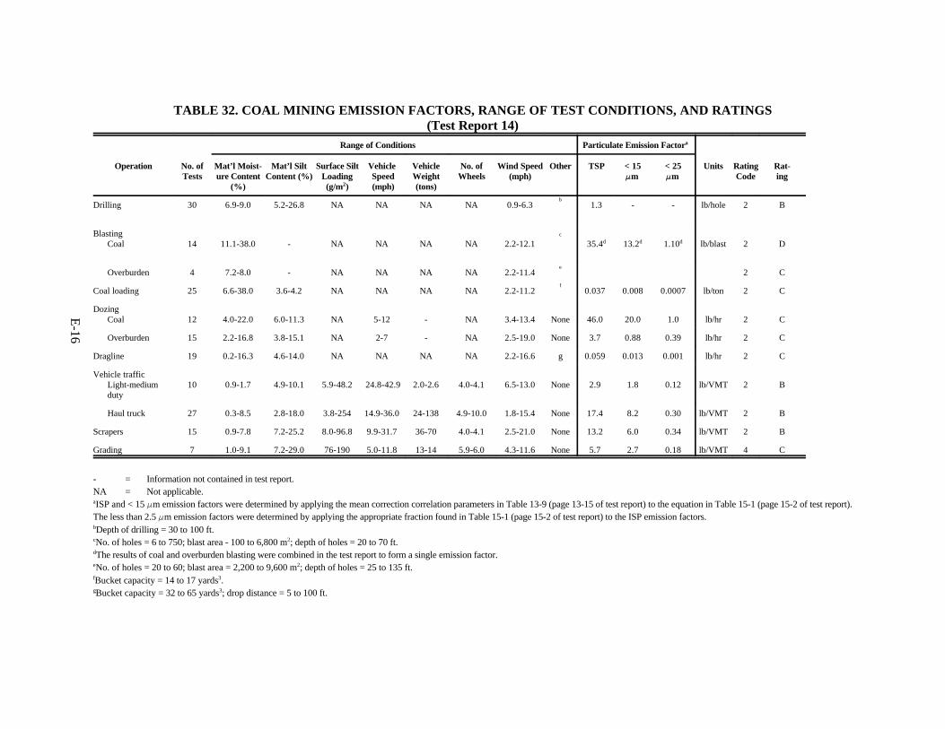
E-16
TABLE 32. COAL MINING EMISSION FACTORS, RANGE OF TEST CONDITIONS, AND RATINGS(Test Report 14)
Range of Conditions Particulate Emission Factora
Operation No. ofTests
Mat’l Moist-ure Content
(%)
Mat’l SiltContent (%)
Surface SiltLoading(g/m2)
VehicleSpeed(mph)
VehicleWeight(tons)
No. ofWheels
Wind Speed(mph)
Other TSP < 15FFm
< 25FFm
Units RatingCode
Rat-ing
Drilling 30 6.9-9.0 5.2-26.8 NA NA NA NA 0.9-6.3b
1.3 - - lb/hole 2 B
BlastingCoal 14 11.1-38.0 - NA NA NA NA 2.2-12.1
c
35.4d 13.2d 1.10d lb/blast 2 D
Overburden 4 7.2-8.0 - NA NA NA NA 2.2-11.4e
2 C
Coal loading 25 6.6-38.0 3.6-4.2 NA NA NA NA 2.2-11.2f
0.037 0.008 0.0007 lb/ton 2 C
DozingCoal 12 4.0-22.0 6.0-11.3 NA 5-12 - NA 3.4-13.4 None 46.0 20.0 1.0 lb/hr 2 C
Overburden 15 2.2-16.8 3.8-15.1 NA 2-7 - NA 2.5-19.0 None 3.7 0.88 0.39 lb/hr 2 C
Dragline 19 0.2-16.3 4.6-14.0 NA NA NA NA 2.2-16.6 g 0.059 0.013 0.001 lb/hr 2 C
Vehicle trafficLight-mediumduty
10 0.9-1.7 4.9-10.1 5.9-48.2 24.8-42.9 2.0-2.6 4.0-4.1 6.5-13.0 None 2.9 1.8 0.12 lb/VMT 2 B
Haul truck 27 0.3-8.5 2.8-18.0 3.8-254 14.9-36.0 24-138 4.9-10.0 1.8-15.4 None 17.4 8.2 0.30 lb/VMT 2 B
Scrapers 15 0.9-7.8 7.2-25.2 8.0-96.8 9.9-31.7 36-70 4.0-4.1 2.5-21.0 None 13.2 6.0 0.34 lb/VMT 2 B
Grading 7 1.0-9.1 7.2-29.0 76-190 5.0-11.8 13-14 5.9-6.0 4.3-11.6 None 5.7 2.7 0.18 lb/VMT 4 C
- = Information not contained in test report.NA = Not applicable.aISP and < 15 Fm emission factors were determined by applying the mean correction correlation parameters in Table 13-9 (page 13-15 of test report) to the equation in Table 15-1 (page 15-2 of test report).The less than 2.5 Fm emission factors were determined by applying the appropriate fraction found in Table 15-1 (page 15-2 of test report) to the ISP emission factors.bDepth of drilling = 30 to 100 ft.cNo. of holes = 6 to 750; blast area - 100 to 6,800 m2; depth of holes = 20 to 70 ft.dThe results of coal and overburden blasting were combined in the test report to form a single emission factor.eNo. of holes = 20 to 60; blast area = 2,200 to 9,600 m2; depth of holes = 25 to 135 ft.fBucket capacity = 14 to 17 yards3.gBucket capacity = 32 to 65 yards3; drop distance = 5 to 100 ft.
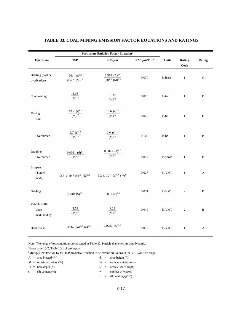
E-17
961 (A)0.8
(D)1.8 (M)1.9
0.119
(M)0.9
78.4 (s)1.2
(M)1.3
5.7 (s)1.2
(M)1.3
1.0 (s)1.5
(M)1.4
0.0021 (d)1.1
(M)0.3
0.0021 (d)0.7
(M)0.3
2.7 x 10&5 (s)1.3 (W)2.4 6.2 x 10&6 (s)1.4 (W)2.5
0.040 (S)2.5 0.051 (S)2.0
5.79
(M)4.0
3.22
(M)4.3
0.0067 (w)3.4 (L)0.2 0.0051 (w)3.5
TABLE 33. COAL MINING EMISSION FACTOR EQUATIONS AND RATINGS
Particulate Emission Factor Equationa
Operation TSP < 15 FFm < 2.5 FFm/TSPb Units Rating
Code
Rating
Blasting (coal or
overburden)
2,550 (A)0.6
(D)1.5 (M)2.30.030 lb/blast 1 C
Coal loading1.16
(M)1.2 0.019 lb/ton 1 B
Dozing
Coal
18.6 (s)1.5
(M)1.4 0.022 lb/hr 1 B
Overburden 0.105 lb/hr 1 B
Dragline
Overburden 0.017 lb/yard3 1 B
Scrapers
(Travel
mode)
0.026 lb/VMT 1 A
Grading 0.031 lb/VMT 2 B
Vehicle traffic
Light-
medium duty
0.040 lb/VMT 2 B
Haul trucks 0.017 lb/VMT 1 A
Note: The range of test conditions are as stated in Table 32. Particle diameters are aerodynamic.aFrom page 15-2, Table 15-1 of test report.bMultiply this fraction by the TSP predictive equation to determine emissions in the < 2.5 Fm size range.
A = area blasted (ft2) d = drop height (ft)
M = moisture content (%) W = vehicle weight (tons)
D = hole depth (ft) S = vehicle speed (mph)
s = silt content (%) w = number of wheels
L = silt loading (g/m2)
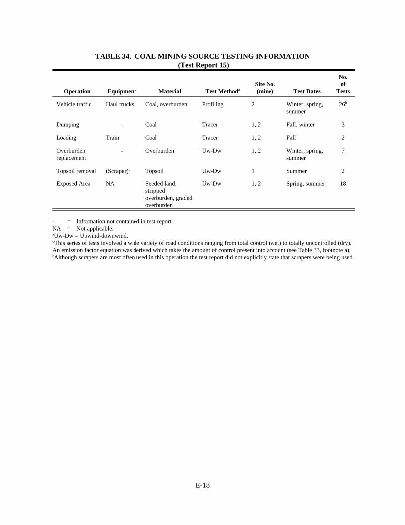
E-18
TABLE 34. COAL MINING SOURCE TESTING INFORMATION (Test Report 15)
Operation Equipment Material Test MethodaSite No.(mine) Test Dates
No.of
Tests
Vehicle traffic Haul trucks Coal, overburden Profiling 2 Winter, spring,summer
26b
Dumping - Coal Tracer 1, 2 Fall, winter 3
Loading Train Coal Tracer 1, 2 Fall 2
Overburdenreplacement
- Overburden Uw-Dw 1, 2 Winter, spring,summer
7
Topsoil removal (Scraper)c Topsoil Uw-Dw 1 Summer 2
Exposed Area NA Seeded land,strippedoverburden, gradedoverburden
Uw-Dw 1, 2 Spring, summer 18
- = Information not contained in test report.NA = Not applicable.aUw-Dw = Upwind-downwind.bThis series of tests involved a wide variety of road conditions ranging from total control (wet) to totally uncontrolled (dry).An emission factor equation was derived which takes the amount of control present into account (see Table 33, footnote a).cAlthough scrapers are most often used in this operation the test report did not explicitly state that scrapers were being used.
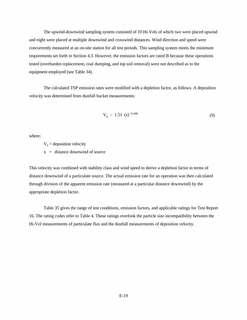
E-19
Vd ' 1.51 (x)&0.588 (9)
The upwind-downwind sampling system consisted of 10 Hi-Vols of which two were placed upwind
and eight were placed at multiple downwind and crosswind distances. Wind direction and speed were
concurrently measured at an on-site station for all test periods. This sampling system meets the minimum
requirements set forth in Section 4.3. However, the emission factors are rated B because these operations
tested (overburden replacement, coal dumping, and top soil removal) were not described as to the
equipment employed (see Table 34).
The calculated TSP emission rates were modified with a depletion factor, as follows. A deposition
velocity was determined from dustfall bucket measurements:
where:
Vd = deposition velocity
x = distance downwind of source
This velocity was combined with stability class and wind speed to derive a depletion factor in terms of
distance downwind of a particulate source. The actual emission rate for an operation was then calculated
through division of the apparent emission rate (measured at a particular distance downwind) by the
appropriate depletion factor.
Table 35 gives the range of test conditions, emission factors, and applicable ratings for Test Report
16. The rating codes refer to Table 4. These ratings overlook the particle size incompatibility between the
Hi-Vol measurements of particulate flux and the dustfall measurements of deposition velocity.
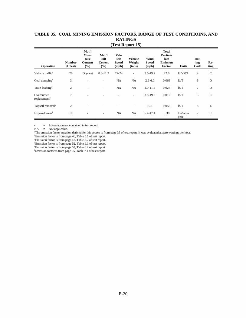
E-20
TABLE 35. COAL MINING EMISSION FACTORS, RANGE OF TEST CONDITIOINS, ANDRATINGS
(Test Report 15)
OperationNumberof Tests
Mat’lMois-ture
Content(%)
Mat’lSilt
Conent(%)
Veh-icle
Speed(mph)
VehicleWeight(tons)
WindSpeed(mph)
TotalParticu-
lateEmission
Factor Units
Rat-ing
CodeRa-ting
Vehicle traffica 26 Dry-wet 8.3-11.2 22-24 - 3.6-19.2 22.0 lb/VMT 4 C
Coal dumpingb 3 - - NA NA 2.9-6.0 0.066 lb/T 6 D
Train loadingc 2 - - NA NA 4.0-11.4 0.027 lb/T 7 D
Overburdenreplacementd
7 - - - - 3.8-19.9 0.012 lb/T 3 C
Topsoil removala 2 - - - - 10.1 0.058 lb/T 8 E
Exposed areasf 18 - - NA NA 5.4-17.4 0.38 ton/acre-year
2 C
- = Information not contained in test report.NA = Not applicable.aThe emission factor equation derived for this source is from page 35 of test report. It was evaluated at zero wettings per hour.bEmission factor is from page 46, Table 5.1 of test report.cEmission factor is from page 47, Table 5.2 of test report.dEmission factor is from page 52, Table 6.1 of test report.eEmission factor is from page 52, Table 6.2 of test report.fEmission factor is from page 55, Table 7.1 of test report.
E-21
8.5 Western Surface Coal Mining and Processing
Since no emission factors are currently presented in AP-42 for coal mining. The predictive
emission factor equations presented in Table 49 are recommended for inclusion in AP-42 under a section
named “Western Surface Coal Mining.” Table 50 presents the single-valued emission factors for western
surface coal mining. It is recommended that for any source operation not covered by the equations in
Table 49, the highest rated single valued factors from Table 50 be incorporated in AP-42.
All of the recommended factors may be applied to Eastern surface coal mining. However, each
should then be aerated one letter value (e.g., C to D).

E-22
961 (A)0.8
(D)1.8 (M)1.9
1.16
(M)1.2 0.119
(M)0.9
78.4 (s)1.2
(M)1.3
18.6 (s)1.5
(M)1.4
5.7 (s)1.2
(M)1.3
1.0 (s)1.5
(M)1.4
0.0021 (d)1.1
(M)0.3
0.0021 (d)0.7
(M)0.3
2.7 x 10&5 (s)1.3 (W)2.4 6.2 x 10&6 (s)1.4 (W)2.5
0.040 (S)2.5 0.051 (S)2.0
5.79
(M)4.0
3.72
(M)4.3
0.0067 (w)3.4 (L)0.2 0.0051 (w)3.5
TABLE 49. WESTERN SURFACE COAL MINING PREDICTIVE EMISSION FACTOR
EQUATIONS
(Test Reports 5 and 14)Particulate Emission Factor Equation
Operation Material TSP < 15 FFm < 2.5FFm/TSPa Units
TestRe-port
Rating
Blasting Coal oroverburden
2,550 (A)0.6
(D)1.5 (M)2.3 0.030 lb/blast 14 C
Truck loading Coal 0.019 lb/ton 14 B
Dozing Coal 0.022 lb/hr 14 B
Overburden 0.105 lb/hr 14 B
Dragline Overburden 0.017 lb/yard3 14 B
Scrapers (travelmode) 0.026 lb/VMT 14 A
Grading 0.031 lb/VMT 14 B
Vehicle traffic(light-mediumduty)
0.040 lb/VMT 14 B
Haul trucks 0.017 lb/VMT 14 A
Storage pile(Winderosion andmaintenance)
Coal 1.6 u - - 5 Cb
- = Unable to be determined from informaiton continaed in test report.aMultiply this fraction by the TSP predictive equation to detemrine emissions in the < 2.5 Fm size range.bRating applicable to Mine Types A, B, and D (see p 61).A = area blasted (ft2) d = drop height (ft)M = moisture content (%) W = vehicle weight (tons)D = hole depth (ft) S = vehicle speed (mph)s = silt content (%) w = number of wheels
F = wind speed (m/sec) L = silt loading (g/m2)
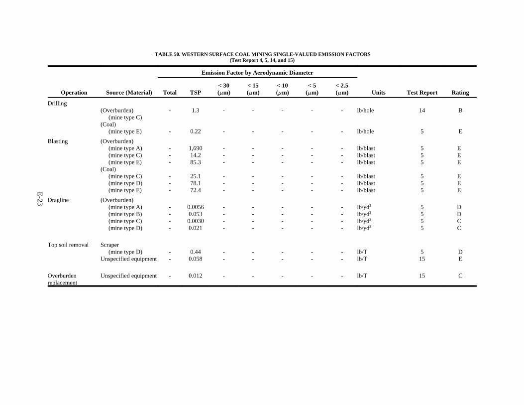
E-23
TABLE 50. WESTERN SURFACE COAL MINING SINGLE-VALUED EMISSION FACTORS(Test Report 4, 5, 14, and 15)
Emission Factor by Aerodynamic Diameter
Operation Source (Material) Total TSP< 30(FFm)
< 15(FFm)
< 10(FFm)
< 5(FFm)
< 2.5(FFm) Units Test Report Rating
Drilling(Overburden)
(mine type C)(Coal)
(mine type E)
-
-
1.3
0.22
-
-
-
-
-
-
-
-
-
-
lb/hole
lb/hole
14
5
B
E
Blasting (Overburden)(mine type A)(mine type C)(mine type E)
(Coal)(mine type C)(mine type D)(mine type E)
---
---
1,69014.285.3
25.178.172.4
---
---
---
---
---
---
---
---
---
---
lb/blastlb/blastlb/blast
lb/blastlb/blastlb/blast
555
555
E*E*E*
E*E*E*
Dragline (Overburden)(mine type A)(mine type B)(mine type C)(mine type D)
----
0.00560.0530.00300.021
----
----
----
----
----
lb/yd3
lb/yd3
lb/yd3
lb/yd3
5555
D*D*C*C*
Top soil removal Scraper(mine type D)
Unspecified equipment--
0.440.058
--
--
--
--
--
lb/Tlb/T
515
DE
Overburdenreplacement
Unspecified equipment - 0.012 - - - - - lb/T 15 C

E-24
TABLE 50. WESTERN SURFACE COAL MINING SINGLE-VALUED EMISSION FACTORS(Test Report 4, 5, 14, and 15) (cont.)
Emission Factor by Aerodynamic Diameter
Operation Source (Material) Total TSP< 30(FFm)
< 15(FFm)
< 10(FFm)
< 5(FFm)
< 2.5(FFm) Units Test Report Rating
Batch-drop Dumping via truck(Overburden-bottom)
(mine type E)(Coal-end)
(mine type E)(Material notspecified-bottom)
(mine type A)(mine type B)(mine type C)(mine type D)
Dumping viascraper (top soil)
(mine type D)Dumping viaunspecifiedequipment orprocess(Coal)(Fly-ash)
(mine type A)Front-endloader/truck(Materialunspecified)
(mine type D)Power shovel/truck(Overburden)
(mine type E)
-
-
----
-
-
-
-
-
0.002
0.007
0.0140.0200.0050.027
0.04
0.066
3.9
0.12
0.037
-
-
----
-
-
-
-
-
-
-
----
-
-
-
-
-
-
-
----
-
-
-
-
-
-
-
----
-
-
-
-
-
-
-
----
-
-
-
-
-
lb/T
lb/T
lb/Tlb/Tlb/Tlb/T
lb/T
lb/T
lb/hr
lb/T
lb/T
5
5
5555
5
15
5
5
5
E
E
DEEE
C
D
E*
E*
C
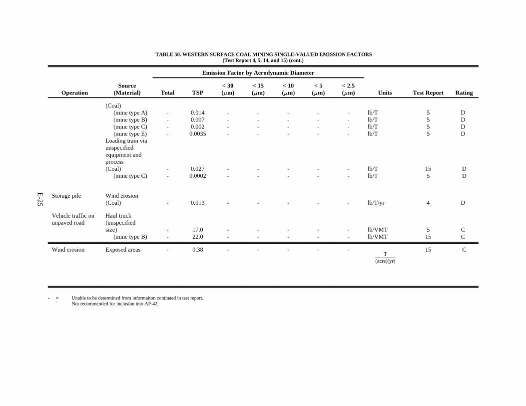
E-25
T(acre)(yr)
TABLE 50. WESTERN SURFACE COAL MINING SINGLE-VALUED EMISSION FACTORS(Test Report 4, 5, 14, and 15) (cont.)
Emission Factor by Aerodynamic Diameter
OperationSource
(Material) Total TSP< 30(FFm)
< 15(FFm)
< 10(FFm)
< 5(FFm)
< 2.5(FFm) Units Test Report Rating
(Coal)(mine type A)(mine type B)(mine type C)(mine type E)
Loading train viaunspecifiedequipment andprocess(Coal)
(mine type C)
----
--
0.0140.0070.0020.0035
0.0270.0002
----
--
----
--
----
--
----
--
----
--
lb/Tlb/Tlb/Tlb/T
lb/Tlb/T
5555
155
D*D*D*D*
DD
Storage pile Wind erosion(Coal) - 0.013 - - - - - lb/T/yr 4 D*
Vehicle traffic onunpaved road
Haul truck(unspecifiedsize)
(mine type B)--
17.022.0
--
--
--
--
--
lb/VMTlb/VMT
515
C*C*
Wind erosion Exposed areas - 0.38 - - - - - 15 C
- = Unable to be determined from informaiton continaed in test report.* = Not recommended for inclusion into AP-42.
E-26
E.2 Memorandum from Chatten Cowherd, MRI, to James Southerland, EPA, June 1986.
MIDWEST RESEARCH INSTITUTE
425 Volker Boulevard
Kansas City, Missouri 64 (cut off)
Telephone (816) 753-(cut off)
June 2, 1986
Mr. James H. Southerland
U.S. Environmental Protection Agency
Office of Air Quality Planning
and Standards
Research Triangle Park, NC 27711
Dear Mr. Southerland:
In response to your recent inquiry, this letter presents our opinion regarding the appropriateness of the emission
factor for blasting as presented in AP-42 Section 8.19.2, Crushed Stone Processing. As noted in the footnote
to Table 8.19.2-2, the subject emission factor was adapted from Table 8.24-2 in the section on Western Surface
Coal Mining, based on tests of coal and overburden blasting at three mines.
A major concern regarding the derivation of this blasting emission factor equation has to do with the moisture
data used to characterize coal. There are only three moisture values (11, 22, 38%) used to represent conditions
for 14 tests at the three mines, and these high values are believed to include bound as well as unbound moisture.
The moisture values of 7.2 and 8.0% used for the our tests of overburden appear to be reasonable.
Another potential concern relates to the fact that the equation was derived mostly from tests of coal. At first
glance, it would seem likely that the techniques for blasting unfractured stone might vary considerably from
E-27
those used for unfractured coal. For example, limited data from Mine 1 indicate that about five times more
explosive is used to blast a given area of overburden as compared to the same area of coal.
In reexamining the original data underlying the equation, we have uncovered a simple relationship between
TSP mass emissions (per blast) and area blasted, as depicted in the attached figure. Except for one
overburden data point for a 135-ft depth of blast, all the coal and overburden data fit this correlation
reasonably well. The depth of blast for coal is consistently about 20 ft. but the depth of blast for
overburden ranges from 20 ft to 70 ft (excluding the outlier point). Although more explosive is required to
blast a given area of overburden (at a typical depth), there appears to be an offsetting effect of lower
friability, so that both overburden and coal fit the same relationship.
Finally, although data on area blasted from the two Monsanto tests of granite and traprock are not
available, we have estimated these values based on Monsanto's calculated quantities of rock blasted and an
assumed depth of 20 ft. As shown on the attached figure the two Monsanto values, which are based on a
much less accurate measurement method, bracket the overall range of mining emission factors for blasting.
Based on the results of this new review of the blasting emission factor equation, we do not recommend that
the emission factor equation originally developed for western surface coal mines be used for stone quarries.
The moisture content data base is inadequate and the values for coal are suspect. Moreover, no significant
dependence of emissions on either moisture content or depth fo blasting (up to 70 ft) is evident.
To estimate TSP emissions from blasting of unfractured stone (assuming the blasting depth does not exceed
70 ft), we recommend the following equation:
e = 0.00050 A1.5
where:
e = TSP emission factor (lb/blast)
A = area blasted (m2)
If the exposed frontal face of the blasted area is of the same magnitude as the top face, it may be
appropriate to use the sum of the frontal and top areas. Note that for relatively small blast areas typical of
rock quarries (<1000 m2), there is more scatter in the supporting data, as shown on the attached figure.

E-28
Please contact me or Dr. Greg Muleski if you have questions about this information.
Sincerely,
MIDWEST RESEARCH INSTITUTE
Chatten Cowherd, Director
Environmental Systems Department
CC/jer
Enclosure

E-29

E-30
E.3 Memorandum from Greg Muleski, MRI, to Frank Noonan, EPA, April 1987
April 3, 1987
Mr. Frank Noonan (MD-14)
Criteria Emissions Section, AMTB, MDAD
Office of Air Quality Planning and Standards
U.S. Environmental Protection Agency
Research Triangle Park, NC 27711
Dear Frank:
Enclosed are the revised copies of the interim guidance and test design drafts we discussed last week.
Please call if you have any questions.
Sincerely,
MIDWEST RESEARCH INSTITUTE
Gregory E. Muleski, Ph.D.
Senior Environmental Engineer
GEM/jer
Enclosure

E-31
DRAFT
INTERIM GUIDANCE FOR ESTIMATING PARTICULATE EMISSIONS
FROM BLASTING OPERATIONS
The U.S. Environmental Protection Agency (EPA) has determined that the AP-42 particulate emission
factor equation for blasting should no longer be applied to coal mines (AP-42 Section 8.24) or stone quarries
(AP-42 Section 8.19.2). The purpose of this document is to provide interim guidance on the estimation of
emissions from blasting operations conducted at western surface coal mines and from operations involving the
blasting of unfractured stone.
Western Surface Coal Mining
The particulate emission factor equation for blasting, which appears in Table 8.24-2, was originally
derived based on 14 tests of coal and 4 tests of overburden at three western surface coal mines. It contains a
strong dependence on moisture content of material blasted. A major concern regarding the derivation of the
equation has to do with the moisture data used to characterize coal. First, problems in obtaining representative
samples of in-place coal were encountered. Second, there are only three moisture values (11, 22, and 38%) used
to represent conditions for 14 tests at the three mines, and these high values are believed to include bound as
well as unbound moisture. The moisture values of 7.2 and 8.0% used for the four tests of overburden appear
to be reasonable.
In reexamining the original data underlying the equation, a simple relationship between TSP mass
emissions (per blast) and area blasted was uncovered, as depicted in Figure 1. Except for one overburden data
point for a 135-ft depth of blast, all the coal and overburden data fit this correlation reasonably well. The depth
of blast for coal is consistently about 20 ft, but the depth of blast for overburden ranges from 20 to 70 ft
(excluding the outlier point). Although more explosive is required to blast a given area of overburden (at a
typical depth), it appears that there may be an offsetting effect of lower friability, so that both overburden and
coal fit the same relationship.
Therefore, to estimate the TSP emissions from blasting of coall or overburden (assuming the blasting
depth does not exceed 70 ft), the following equation is recommended:

E-32
e = 0.00050 A1.5
where:
e = TSP emission factor (lb/blast)
A = area blasted (m2)
The area blasted (A) refers to the horizontal area and does not include the vertical face of a bench. For
example, if a blast employs M rows (separated by a distance x meters) of N holes separated by a distance y
meters, then the area blasted by the (M@N) holes is (M@N@x@y) square meters.
In order to estimate PM10 emissions (#10µmA) from blasting, the value obtained from Equation 1 for
TSP emissions (#30µmA) should be multiplied by 0.5. This value represents and average PM10/PM30 ratio
derived from teh materials handling particle size data currently presented in Section 11.2.3 of AP-42. The
PM10 size fraction was not quantified directly in the study of blasting emissions from western surface coal
mines.
The quality rating for the new emission factor equation may be derived in the same manner as was done
for the quation for blasting currently given in Section 8.24, Western Surface Coal Mining. As stated in the
supporting background document (EPA-450/4-83-003), the blasting test data from teh western suface coal
mines are rated C. According t the quality rating criteria for emission factor equations, there is no reduction
of qualty rating (i.e., the equation is also rated C) if used to estimate blasting emissions in western surface coal
mines.
Crushed Stone Processing
Only two single-valued emission factors for blasting of unfractured stone appear in the literature. As
indicated in the background document for Section 8.19, Construction Aggregate (EPA-450/4-83-007), the
single-valued emission factors for blasting of granite and traprock are both rated E (poor). The principal reason
for the low rating of these factors is the small number of supporting tests (one or two) for each factor, even
though the test data from these “screening studies” are rated B in both cases.
The new emission factor equation presented above for coal and over-burden blasting at western surface
coal mines provides a possible alternative to the single-valued emission factors for estimation of particulate

E-33
emissions from blasting operation at stone quarries. As stated above, the emission factor equation carries a C
quality rating if applied to western surface coal mines. For application to similar blasting operations in other
industries, the equation would be rated D provided that: (a) reliable values of the correction parameters have
been determined for the specific sources of interest; and (b) the correction parameter values are with in ranges
tested in developing the equation. Because of typical dissimilarities in the techniques used for blasting in
western surface coal mines as compared to stone quarries, there is ample reason for further reducing the rating
of the emission factor equation to E for application to blasting of unfractured stone. In particular most stone
quarries involve relatively small blast areas (A < 1000 m2), which bracket the lower end of the range shown
in Figure 1 for western surface coal mines. Moreover, it can be seen in Figure 1 that the scatter in the data for
blast areas smaller than about 2000 m2 indicate a decrease in reliability of the equation even when applied to
western surface coal mines.
Therefore, it is concluded that for a wide range of industrial applications involving blasting of
unfractured stone, the single-valued emission factors as well as the newly develop emission factor equation
yield only crude estimates (E-rated) of particulate emissions. At this low degree of quantitation, it is difficult
to reason as to which estimate is more reliable. Unfortunately, in the absence of much needed additional test
data, the investigator must deal with the problem of selecting the most appropriate emission factor on a case-
by-case basis.
It is strongly recommended that reliable emission factors for estimated particulate emissions from
blasting of unfractured stone be based on site specific field testing. The attachment Design of Field Studies
of Blasting Emissions, presents applicable guidance on available sampling methods, sampling devices, and test
design considerations.

E-34
E.4 Section 9 of "Improved Emission Factors For Fugitive Dust From Western Surface Coal Mining
Sources--Volume I - Sampling methodology and Test Results."
SECTION 9
RESULTS FOR SOURCE TESTED BY BALLOON SAMPLING
SUMMARY OF TESTS PERFORMED
Blasting was the only source tested by the balloon sampling method. Overburden and coal blasts
were both sampled with the same procedure, but the data were kept separate during the data analysis phase
so that the option of developing separate emission factors was available. A total of 18 successful tests were
completed--14 for coal blasts and 4 for overburden blasts. Three more blasts were sampled, but the balloon
was hit and broken in one and the plumes missed the sampler arrays in two others; no attempt was made to
calculate emission rates for these three tests.
The overburden was not blasted at the mine in North Dakota (second mine), so overburden blast
tests were confined to the first and third mines. The resulting sample size of four is not large enough for
development of a-statistically sound emission factor.
The sampling array consisted of balloon-supported samplers at five heights plus five pairs of
ground-based hi-vols and dichots to establish the horizontal extent of the plume. No measure of deposition
rate was made with this configuration because all samplers were at the same distance from the source.
Samplers at Mine 2 were located in the pit for coal blasts, but samplers at Mines 1 and 3 were
located on the highwall above the pit. Therefore, some (prior) deposition is included in the emission rate
measured at the latter mines. These are the only emission rates in the study that are not representative of
emissions directly from the source.
Test conditions for the blasting tests are summarized in Table 9-1. An extremely wide range of
blast sizes was sampled--from 6 to 750 holes and from 100 to 9600 m2. The variation in moisture contents
was also quite wide. The only potential correction factor with a limited range during testing was the depth
of the holes. All the holes for coal blasts were about 20 ft deep. Overburden holes had a range of 25 to
135 ft. but there are not enough data points to develop a correction factor.

E-35
TABLE 9-1. TEST CONDITIONS FOR BLASTING
Sampling Conditions Source CharacteristicsSoil
Properties Meteorological Conditions
Test Date Start TimeDuration,Minutes
SamplersIn or Out
of PitNo. ofHoles Area m2
Tons ofExplosive
Depth ofHoles, ft.
Moisture,%
Temp.,EEF
WindSpeed, m/s Stab Class
Mine 1
Coal 123
8/10/798/10/798/14/79
15:0015:3012:00
537
outoutout
336
42
1100100
1600
1.00.21.3
222220
222222
828262
1.11.01.4
AAB
Ovb 12
8/14/798/20/79
14:3014:45
168
outout
3320
34002200
12.010.0
7060
7.27.2
6676
5.12.0
DA
Mine 2
Coal 123456
10/25/7910/26/7910/29/7910/29/7910/29/7910/30/79
11:2811:009:33
12:0714:3014:35
683676
inininininin
195210180150110
96
110011001000
8001100
600
202020202020
383838383838
454343433847
2.61.61.81.03.25.4
CCCBDD
Mine 3
Coal 23456
7/28/807/29/808/01/808/04/808/06/80
14:2014:1013:1014:1510:45
1321257
12
outoutoutoutout
250750200150160
41006800340024002700
2020202020
11.111.111.111.111.1
99104909582
1.71.22.02.71.3
BBACB
Ovb 12
8/06/808/12/80
14:3515:05
1010
outout
5060
96005000
13525
8.08.0
9395
1.71.0
AA
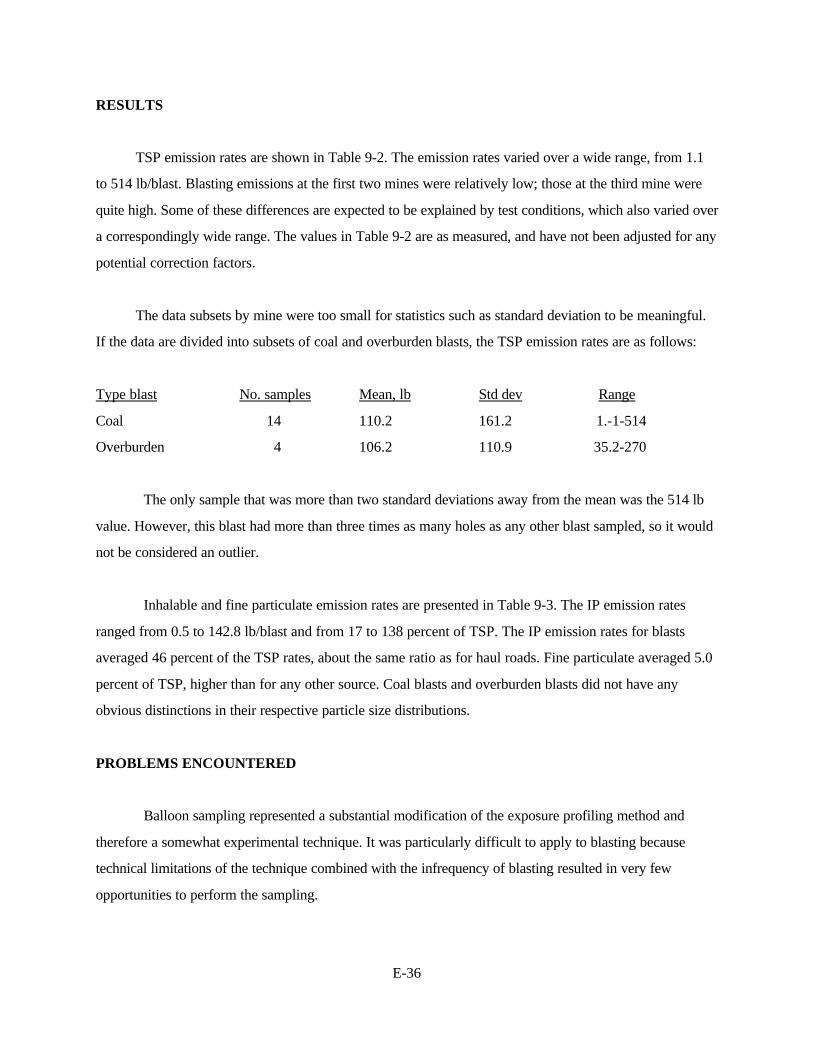
E-36
RESULTS
TSP emission rates are shown in Table 9-2. The emission rates varied over a wide range, from 1.1
to 514 lb/blast. Blasting emissions at the first two mines were relatively low; those at the third mine were
quite high. Some of these differences are expected to be explained by test conditions, which also varied over
a correspondingly wide range. The values in Table 9-2 are as measured, and have not been adjusted for any
potential correction factors.
The data subsets by mine were too small for statistics such as standard deviation to be meaningful.
If the data are divided into subsets of coal and overburden blasts, the TSP emission rates are as follows:
Type blast No. samples Mean, lb Std dev Range
Coal 14 110.2 161.2 1.-1-514
Overburden 4 106.2 110.9 35.2-270
The only sample that was more than two standard deviations away from the mean was the 514 lb
value. However, this blast had more than three times as many holes as any other blast sampled, so it would
not be considered an outlier.
Inhalable and fine particulate emission rates are presented in Table 9-3. The IP emission rates
ranged from 0.5 to 142.8 lb/blast and from 17 to 138 percent of TSP. The IP emission rates for blasts
averaged 46 percent of the TSP rates, about the same ratio as for haul roads. Fine particulate averaged 5.0
percent of TSP, higher than for any other source. Coal blasts and overburden blasts did not have any
obvious distinctions in their respective particle size distributions.
PROBLEMS ENCOUNTERED
Balloon sampling represented a substantial modification of the exposure profiling method and
therefore a somewhat experimental technique. It was particularly difficult to apply to blasting because
technical limitations of the technique combined with the infrequency of blasting resulted in very few
opportunities to perform the sampling.

E-37
TABLE 9-2. APPARENT EMISSION RATES FOR BLASTINGHigh-Volume (30 FFm)
Test No. Pound/BlastDistance from
Source, m Test No. Pound/BlastDistance from
Source, m
Mine 1Coal
123
32.52.7
51.7
969637
Mine 1Overburden
12
40.479.4
100100
Mine 2Coal
123456
8.81.1
10.71.6
40.311.8
130213130160170180
Mine 3Coal
23456
401514148113206
901601285382
Mine 3Overburden
12
35.2270
110200

E-38
TABLE 9-3. APPARENT EMISSION RATES FOR BLASTINGDichotomous (15 FFm, 2.5 FFm)
Test No.
Pound/BlastDistance
fromSource, m Test No.
Pound/Blast
Distance fromSource, mIP FP IP FP
Mine 1Coal
123
44.9a
1.5617.3
3.620.321.23
969637
Mine 1Overburden
12
32.948.9
0.790.09
100100
Mine 2Coal
123456
1.550.623.570.45
15.301.99
0.100.060.800.101.270.01
130213130160170180
Mine 3Coal
23456
123.4142.887.935.371.3
10.412.313.02.1
19.8
901601285382
Mine 3Overburden
12
16.993.9
3.516.2
110200
aDichotomous concentrations are greater than hi-vol, value represents 20.5µm cut point for IP.

E-39
This sampling method could not be used when ground level winds were greater than about 6 m/s
because the balloon could not be controlled on its tether. At wind speeds less than about 1 m/s, wind
direction tended to vary and the sampling array could not be located with any confidence of being in the
plume. Also, at low wind speeds, the plume from the blast frequently split or rose vertically from the blast
site. Therefore, sampling was constrained to a fairly narrow range of wind speeds.
For safety reasons, a source-sampler distance of 100 m or more was usually required. At this
distance, the plume could disperse vertically above the top sampler inlet under unstable atmospheric
conditions.
Even though sampling was done at very large mines, only one or two blasts per day were
scheduled. This often created difficulties in obtaining the prescribed number of blasting tests at each mine.
Since blasting was not a continuous operation, there was no continuous plume to provide
assistance in locating the samplers. For coal blasts in particular, the portion of the plume below the high
wall usually was channeled parallel to the pit but any portion rising above the high wall was subject to
ambient winds and often separated from the plume in the pit.
Finally, representative soil samples could not be obtained for this source because of the abrupt
change in the characteristics of the soil caused by the blast. The moisture contents reported in Table 9-1
were for samples of coal in place and overburden from drilling tests (both prior to blasting).

F-1
Appendix FMaterials Related to Truck Loading, Bulldozing, and Dragline
Emission Factors
This appendix contains information related to truck loading, bulldozing and dragline emission
factors. The information is from Sections 5.5 and 8.5 of EPA report “Fugitive Dust Emission Factor
Update for AP42 ” and Section 8 of EPA report “Improved Emission Factors For Fugitive Dust From
Western Surface Coal Mining Sources - Volume I - Sampling Methodology and Test Results.”
F-2
TABLE OF CONTENTS
Page
F.1 Sections 5.5 and 8.5 of EPA report "Fugitive Dust Emission Factor Update for AP-42" . . . . . . . . . . . . . . . . . . . . . . . . . . . . . . . . . . . . . . . . . . . . . . . . F-3
F.2 Section 8 of EPA report "Improved Emission Factors for Fugitive Dust fromWestern Surface Coal Mining Sources--Volume I - Sampling Methodology and Test Results . . . . . . . . . . . . . . . . . . . . . . . . . . . . . . . . . . . . . . . . . . . . . . . . . . F-25
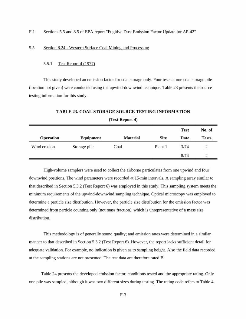
F-3
F.1 Sections 5.5 and 8.5 of EPA report "Fugitive Dust Emission Factor Update for AP-42"
5.5 Section 8.24 - Western Surface Coal Mining and Processing
5.5.1 Test Report 4 (1977)
This study developed an emission factor for coal storage only. Four tests at one coal storage pile
(location not given) were conducted using the upwind-downwind technique. Table 23 presents the source
testing information for this study.
TABLE 23. COAL STORAGE SOURCE TESTING INFORMATION
(Test Report 4)
Operation Equipment Material Site
Test
Date
No. of
Tests
Wind erosion Storage pile Coal Plant 1 3/74 2
8/74 2
High-volume samplers were used to collect the airborne particulates from one upwind and four
downwind positions. The wind parameters were recorded at 15-min intervals. A sampling array similar to
that described in Section 5.3.2 (Test Report 6) was employed in this study. This sampling system meets the
minimum requirements of the upwind-downwind sampling technique. Optical microscopy was employed to
determine a particle size distribution. However, the particle size distribution for the emission factor was
determined from particle counting only (not mass fraction), which is unrepresentative of a mass size
distribution.
This methodology is of generally sound quality; and emission rates were determined in a similar
manner to that described in Section 5.3.2 (Test Report 6). However, the report lacks sufficient detail for
adequate validation. For example, no indication is given as to sampling height. Also the field data recorded
at the sampling stations are not presented. The test data are therefore rated B.
Table 24 presents the developed emission factor, conditions tested and the appropriate rating. Only
one pile was sampled, although it was two different sizes during testing. The rating code refers to Table 4.

F-4
TABLE 24. COAL STORAGE EMISSION FACTOR, RANGE OF TEST CONDITIONS,AND RATING(Test Report 4)
Range of Conditions
OperationNo. ofTests
WindSpeed(m/S)
MoistureContent
(%)EmissionFactora,b
RatingCode Rating
Wind erosion ofcoal storage pile
4 1.5-2.7 2.2-111 0.013lb/T/yr
5 D
aFor particles < 10 Fm (physical diameter).
bEmission factor is arithmetic mean of test runs C1, C2, CS-3 and CS-5 from page 30, Table A1 of test report.
5.5.2 Test Report 5 (1978)
This study was directed to the development of emission factors for the surface coal mining
industry. Testing was conducted at five Western coal mines (Mines A through E). Table 25 presents the
distribution of tests performed.
The upwind-downwind method was used with standard high-volume samplers for particulate
collection. Wind parameters were continuously measured at a fixed location within each mine. A hand-held
wind speed indicator was used when possible to record data at the exact test site. Optical microscopy was
employed to determine particle size distribution.
The upwind-downwind sampler deployment used in this study generally employed six samplers for
each test; additionally, six more samplers were operated at a second height in half the tests to determine a
vertical plume gradient. Two instruments were located upwind of a source to measure background
concentrations while four instruments were located downwind. These downwind samplers were deployed
along a straight line (the assumed plume centerline) at four different distances.
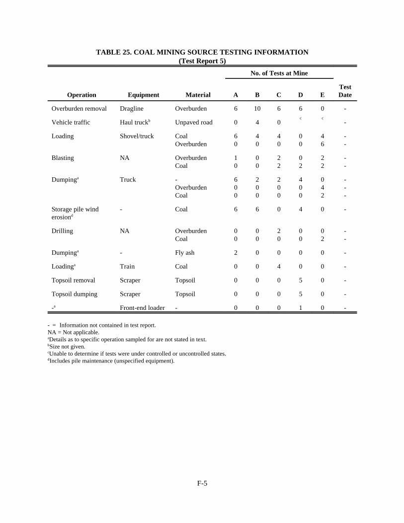
F-5
TABLE 25. COAL MINING SOURCE TESTING INFORMATION(Test Report 5)
No. of Tests at Mine
Operation Equipment Material A B C D ETestDate
Overburden removal Dragline Overburden 6 10 6 6 0 -
Vehicle traffic Haul truckb Unpaved road 0 4 0c c
-
Loading Shovel/truck CoalOverburden
60
40
40
00
46
--
Blasting NA OverburdenCoal
10
00
22
02
22
--
Dumpinga Truck -OverburdenCoal
600
200
200
400
042
---
Storage pile winderosiond
- Coal 6 6 0 4 0 -
Drilling NA OverburdenCoal
00
00
20
00
02
--
Dumpinga - Fly ash 2 0 0 0 0 -
Loadinga Train Coal 0 0 4 0 0 -
Topsoil removal Scraper Topsoil 0 0 0 5 0 -
Topsoil dumping Scraper Topsoil 0 0 0 5 0 -
-a Front-end loader - 0 0 0 1 0 -
- = Information not contained in test report.NA = Not applicable.aDetails as to specific operation sampled for are not stated in text.bSize not given.cUnable to determine if tests were under controlled or uncontrolled states.dIncludes pile maintenance (unspecified equipment).

F-6
C 'Q
BFyFzu(6)
The determination of emission rates involved back calculation using dispersion equations after
subtraction of the background from the downwind concentration. The following dispersion equation was
where:
C = concentration
Q = emission rate
Fy,Fz = horizontal and vertical dispersion coefficients
u = wind speed
Line source emission rates were determined by use of this dispersion equation:
C '2 Q
sin N 2B Fz u(7)
where:
C = concentration
Q = emission rate
N = angle between line source and wind direction
Fz = vertical dispersion coefficient
u = wind speed
The predictive emission factor equation for wind erosion of active storage piles was developed by
plotting the emission rates against the wind speeds recorded during testing. The resulting linear function was
described by the equation:
e ' 15.83 u (8)
where:
e = emission rate (lb/hr)
u = wind speed (m/sec)
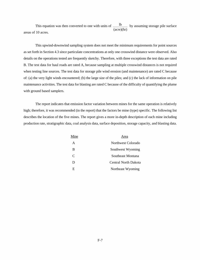
F-7
This equation was then converted to one with units of by assuming storage pile surfacelb(acre)(hr)
areas of 10 acres.
This upwind-downwind sampling system does not meet the minimum requirements for point sources
as set forth in Section 4.3 since particulate concentrations at only one crosswind distance were observed. Also
details on the operations tested are frequently sketchy. Therefore, with three exceptions the test data are rated
B. The test data for haul roads are rated A, because sampling at multiple crosswind distances is not required
when testing line sources. The test data for storage pile wind erosion (and maintenance) are rated C because
of: (a) the very light winds encountered; (b) the large size of the piles; and (c) the lack of information on pile
maintenance activities. The test data for blasting are rated C because of the difficulty of quantifying the plume
with ground based samplers.
The report indicates that emission factor variation between mines for the same operation is relatively
high; therefore, it was recommended (in the report) that the factors be mine (type) specific. The following list
describes the location of the five mines. The report gives a more in-depth description of each mine including
production rate, stratigraphic data, coal analysis data, surface deposition, storage capacity, and blasting data.
Mine Area
A Northwest Colorado
B Southwest Wyoming
C Southeast Montana
D Central North Dakota
E Northeast Wyoming

F-8
Tables 26 through 30 present the average emission factors determined at each mine along with the
ranges of conditions tested and the associated emission factor ratings. The text indicates that the emission
factors should be used with a fallout function for distances closer than 5 km; however, the text does not
explicitly state what particulate size range is represented by the emission factors.
The rating codes in Tables 26 through 30 refer to Table 5 (wind erosion) and Table 4 (all other
sources). Because the single-valued factors were intended to apply only to the specific mine types, the
requirement for more than one test site was waived. The rating for the equation developed for storage pile wind
erosion (and maintenance) is applicable when the equation is applied to mine types A, B. or D.
5.5.3 Test Report 14 (1981)
This study was conducted to determine improved fugitive dust emission factors for Western surface
coal mines. Field testing was conducted in three coal fields; Powder River Basin (Mine 1), North Dakota (Mine
2), and Four Corners (Mine 3). The testing was performed during 1979 and 1980. Table 31 lists the testing
information for this study.
The primary sampling method was exposure profiling. When source configuration made it necessary,
alternate methods were used, including upwind-downwind, balloon, and quasi-stack sampling. Particle size
distributions were determined by use of dichotomous samplers. Other equipment utilized were: (a) high volume
samplers for determining upwind concentrations; (b) dustfall buckets for determining downwind particulate
deposition; and © recording wind instruments to determine mean wind speed and direction for adjusting the
exposure profiler to isokinetic sampling conditions and for use in upwind-downwind calculations.
Exposure profiling was used to measure emissions from moving point sources (see Table 31). The
exposure profiling sampling system was similar to that described in Section 5.1.1 and therefore meets the
minimum system design requirements. The upwind-downwind sampling system consisted generally of 15
particulate collection devices; 5 dichotomous samplers and 10 Hi-vols.
One Hi-Vol and one dichotomous sampler were placed upwind while the remaining instruments were
placed at multiple downwind and crosswind distances. This system also meets the minimum upwind-downwind
requirements as described in Section 4.3.

F-9
TABLE 26. COAL MINING EMISSION FACTORS (MINE TYPE A), RANGE OF TESTCONDITIONS, AND RATINGS
(Test Report 5)
Range of Conditions
OperationNumberof Tests
Wind Speed(mph) Moisture (%)
TSP EmissionFactora,b
RatingCode Rating
Dragline 6 0.4-1.8 - 0.0056 lb/yd3 4 D
Shovel/truck loading(coal)
6 0.4-1.3 10 0.014 lb/T 4 D
Blasting (overburden) 1 2.4 - 1,690c lb/blast 9 E
Truck dumpd
(bottom)6 0.4-2.7 - 0.014 lb/T 4 D
Storage pile erosione 6 0.5-2.6 10 1.6 u lb(acre)(hr)
1f Cf
Fly ash dump 2 1.5 - 3.9 lb/hr 7/8 E
- = Information not contained in test report.aParticle size not explicitly stated in test report.bEmission factors are from page 2, Table 1 of test report.cText indicates this value represents a maximum rate.dMaterial not given.eu = Wind speed in m/sec. This factor includes emissions from pile maintenance.fRating code refers to Table 5. Rating based on combined data Mines A, B, and D.

F-10
TABLE 27. COAL MINING EMISSION FACTORS (MINE TYPE B), RANGE OF TESTCONDITIONS, AND RATINGS
(Test Report 5)
Range of Conditions
OperationNumberof Tests
Wind Speed(mph) Moisture (%)
TSP EmissionFactora,b
RatingCode Rating
Dragline 10 3.1-5.8 - 0.053 lb/yd3 4 D
Haul road 4 3.7-4.7 - 17.0 lb/VMT 5 C
Shovel/truck loading(coal)
4 0.4-0.6 18 0.007 lb/T 5 D
Truck dump(bottom)
2 3.7 - 0.020 lb/T 7 E
Storage pile erosionc 6 0.8-7.6 18 1.6 u lb(acre)(hr)
1d Cd
- = Information not contained in test report.aParticle size not explicitly stated in test report.bEmission factors are from page 2, Table 1 of test report.cu = Wind speed in m/sec. This factor includes emissions from pile maintenance.dRating code refers to Table 5. Rating based on combined data Mines A, B, and D.

F-11
TABLE 28. COAL MINING EMISSION FACTORS (MINE TYPE C), RANGE OF TESTCONDITIONS, AND RATINGS
(Test Report 5)
Range of Conditions
OperationNumberof Tests
Wind Speed(mph) Moisture (%)
TSP EmissionFactora,b
RatingCode Rating
Dragline 6 3.6-5.4 - 0.0030 lb/yd3 3 C
Shovel/truck loading(coal)
4 3.6 24 0.002 lb/T 5 D
BlastingCoal 2 5.4 24 25.1 lb/blast 7 E
Overburden 2 3.6 - 14.2 lb/blast 7 E
Truck dump (bottom) 2 3.6 - 0.005 lb/T 7 E
Drilling (overburden) 2 3.6 - 1.5 lb/hole 8
Train loading 4 4.5-4.9 24 0.0002 lb/T 5 D
- = Information not contained in test report.aParticle size not explicitly stated in test report.bEmission factors are from page 2, Table 1 of test report.
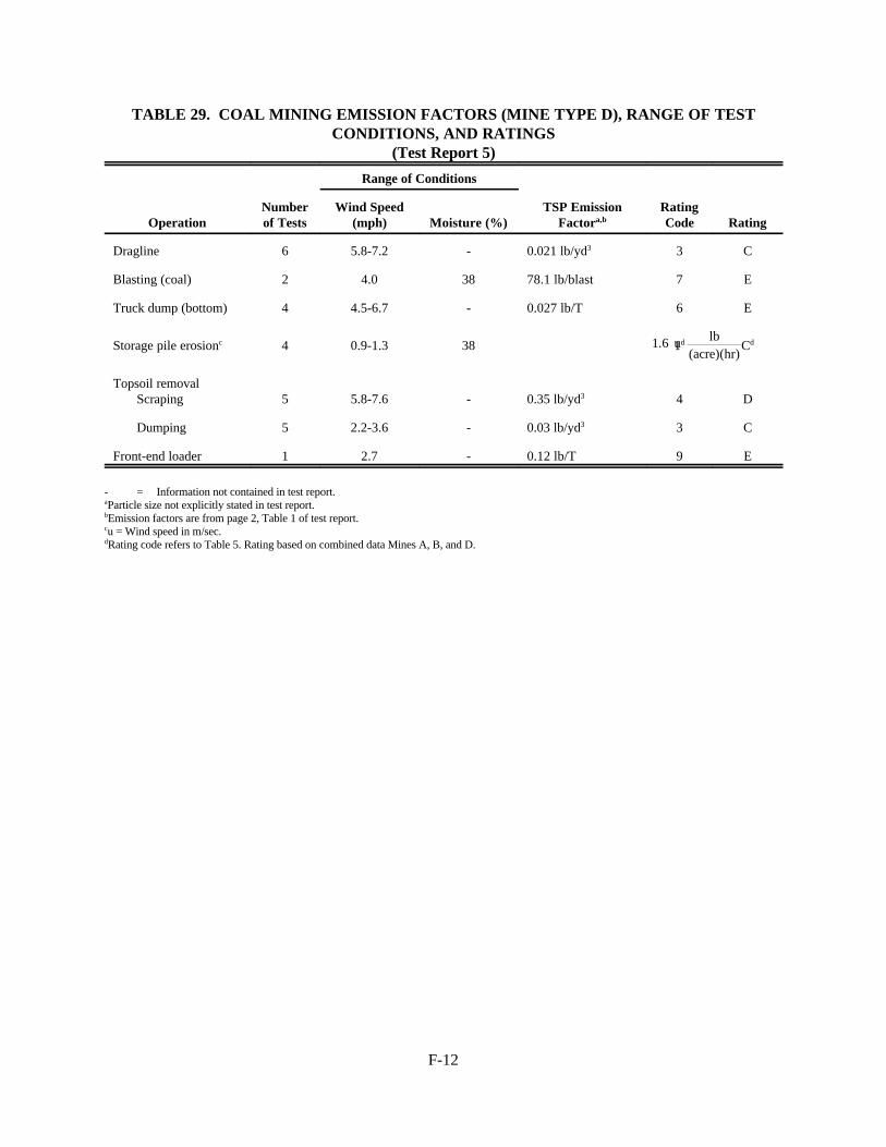
F-12
TABLE 29. COAL MINING EMISSION FACTORS (MINE TYPE D), RANGE OF TESTCONDITIONS, AND RATINGS
(Test Report 5)
Range of Conditions
OperationNumberof Tests
Wind Speed(mph) Moisture (%)
TSP EmissionFactora,b
RatingCode Rating
Dragline 6 5.8-7.2 - 0.021 lb/yd3 3 C
Blasting (coal) 2 4.0 38 78.1 lb/blast 7 E
Truck dump (bottom) 4 4.5-6.7 - 0.027 lb/T 6 E
Storage pile erosionc 4 0.9-1.3 38 1.6 u lb(acre)(hr)
1d Cd
Topsoil removalScraping 5 5.8-7.6 - 0.35 lb/yd3 4 D
Dumping 5 2.2-3.6 - 0.03 lb/yd3 3 C
Front-end loader 1 2.7 - 0.12 lb/T 9 E
- = Information not contained in test report.aParticle size not explicitly stated in test report.bEmission factors are from page 2, Table 1 of test report.cu = Wind speed in m/sec.dRating code refers to Table 5. Rating based on combined data Mines A, B, and D.

F-13
TABLE 30. COAL MINING EMISSION FACTORS (MINE TYPE E), RANGE OF TESTCONDITIONS, AND RATINGS
(Test Report 5)
Range of Conditions
OperationNumberof Tests
Wind Speed(mph) Moisture (%)
TSP EmissionFactora,b
RatingCode Rating
Shovel/truck loadingCoal 4 2.3-2.5 30 0.0035 lb/T 5 D
Overburden 6 2.7-3.6 30 0.037 lb/T 3 C
BlastingCoal
2 2.6 30 72.4 lb/blast 7 E
Overburden 2 3.7 - 85.3 lb/blast 7 E
Truck dumpOverburden
2 6.2 - 0.002 lb/T 8 E
Coal (end dump) 4 2.7-3.1 30 0.007 lb/T 6 E
Drilling (coal) 2 4.1 30 0.22 lb/hole 8 E
- = Information not contained in test report.aParticle size not explicitly stated in test report.bEmission factors are from page 2, Table 1 of test report.

F-14
TABLE 31. COAL MINING SOURCE TESTING INFORMATION (Test Report 14)
Operation Equipment Material Test Methoda Site (mine) Test Dates
No.of
Tests
Drilling NA Overburden Quasi-stack 1, 3 7/79, 8/79,12/79, 7/80
30
Blasting NA Coal Balloonb 1, 2, 3 8/79,10/79,7/80, 8/80
14
Overburden Balloonb 1, 3 8/79, 8/80 4
Loading Shovel/truck Coal Uw-Dw 1, 2 8/79, 10/79 10
Front-endloader/truck
Coal Uw-Dw 3 7/80, 8/80 15
Dozing Dozer Coal Uw-Dw 1, 2, 3 8/79, 10/79,8/80
12
Overburden Uw-Dw 1, 2, 3 8/79, 10/79,7/80, 8/80
15
Dragline Dragline Overburden Uw-Dw 1, 2, 3 8/79, 10/79,7/80, 8/80
19
Vehicle traffic Haul truck Unpaved road Uw-Dw 1 8/79, 12/79 11
Unpaved road Profiling 1, 2 ,3 7/79, 8/79,12/79
21
Light-medium duty
Unpaved road Profiling 1, 2, 3 8/79, 10/79,8/80
10
Scrapersc (travel mode)
Scraper Unpaved surface Uw-Dw 1 7/79 5
Unpaved surface Profiling 1, 2, 3 7/79, 10/79,12/79, 8/80
15
Grading Grader Unpaved surface Profiling 2, 3 10/79, 8/80 7
- = Information not contained in test report.NA = Not applicable.aUw-Dw = Upwind-downwind.bThis is actually a modified version of exposure profiling.cLoading and dumping not tested.

F-15
The test data were collected using a well documented sound methodology and, therefore, are rated
A for line sources and for drilling. The test data for coal loading, dozing, and dragline operations are rated
B because of the poorly defined plume characteristics and the interference of the pit areas with plume
dispersion. For blasting the test data are rated C because of the difficulty of quantifying the large plume
with a single line of samplers.
Table 32 presents the average emission factors, range of test conditions, and ratings assigned for
Test Report 14. These single-valued factors were determined by substituting geometric means of the test
conditions into a set of predictive emission factor equations also developed in the study. The equations are
listed in Table 33. The rating codes in Table 32 refer to Table 4, and the codes in Table 33 refer to Table
5.
5.5.4 Test Report 15 (1981)
A portion of this study was devoted to the development of surface coal mining emission factors.
Field testing was performed from August 1978 through the summer of 1979 at two surface coal mines
located in the Powder River Basin of Wyoming. Table 34 presents the source testing information for this
study.
The test methods employed to develop emission factors were: upwind-downwind, profiling, and a
tracer technique. Particle sizing was performed by optical microscopy of exposed Millipore filters.
The profiling technique employed in this study was actually a variation of the exposure profiling
procedure described in Section 5.1.1 (Test Report 7). High volume samplers were used instead of
directional isokinetic intakes; therefore, the emission rates determined by profiling were for TSP (total
suspended particulate).
The tracer technique utilized arrays of bcch high-volume samplers and tracer samplers with a
straightforward calculation scheme. These sampling systems meet the minimum requirements as set forth in
Section 4.3; therefore; the test data are rated A.

F-16
TABLE 32. COAL MINING EMISSION FACTORS, RANGE OF TEST CONDITIONS, AND RATINGS(Test Report 14)
Range of Conditions Particulate Emission Factora
Operation No. ofTests
Mat’l Moist-ure Content
(%)
Mat’l SiltContent (%)
Surface SiltLoading(g/m2)
VehicleSpeed(mph)
VehicleWeight(tons)
No. ofWheels
Wind Speed(mph)
Other TSP < 15FFm
< 25FFm
Units RatingCode
Rat-ing
Drilling 30 6.9-9.0 5.2-26.8 NA NA NA NA 0.9-6.3 b 1.3 - - lb/hole 2 B
BlastingCoal 14 11.1-38.0 - NA NA NA NA 2.2-12.1 c 35.4d 13.2d 1.10d 2 D
Overburden 4 7.2-8.0 - NA NA NA NA 2.2-11.4 e lb/blast 2 C
Coal loading 25 6.6-38.0 3.6-4.2 NA NA NA NA 2.2-11.2 f 0.037 0.008 0.0007 lb/ton 2 C
DozingCoal 12 4.0-22.0 6.0-11.3 NA 5-12 - NA 3.4-13.4 None 46.0 20.0 1.0 lb/hr 2 C
Overburden 15 2.2-16.8 3.8-15.1 NA 2-7 - NA 2.5-19.0 None 3.7 0.88 0.39 lb/hr 2 C
Dragline 19 0.2-16.3 4.6-14.0 NA NA NA NA 2.2-16.6 g 0.059 0.013 0.001 lb/hr 2 C
Vehicle trafficLight-mediumduty
10 0.9-1.7 4.9-10.1 5.9-48.2 24.8-42.9 2.0-2.6 4.0-4.1 6.5-13.0 None 2.9 1.8 0.12 lb/VMT 2 B
Haul truck 27 0.3-8.5 2.8-18.0 3.8-254 14.9-36.0 24-138 4.9-10.0 1.8-15.4 None 17.4 8.2 0.30 lb/VMT 2 B
Scrapers 15 0.9-7.8 7.2-25.2 8.0-96.8 9.9-31.7 36-70 4.0-4.1 2.5-21.0 None 13.2 6.0 0.34 lb/VMT 2 B
Grading 7 1.0-9.1 7.2-29.0 76-190 5.0-11.8 13-14 5.9-6.0 4.3-11.6 None 5.7 2.7 0.18 lb/VMT 4 C
- = Information not contained in test report.NA = Not applicable.aISP and < 15 Fm emission factors were determined by applying the mean correction correlation parameters in Table 13-9 (page 13-15 of test report) to the equation in Table 15-1 (page 15-2 of test report).The less than 2.5 Fm emission factors were determined by applying the appropriate fraction found in Table 15-1 (page 15-2 of test report) to the ISP emission factors.bDepth of drilling = 30 to 100 ft.cNo. of holes = 6 to 750; blast area - 100 to 6,800 m2; depth of holes = 20 to 70 ft.dThe results of coal and overburden blasting were combined in the test report to form a single emission factor.eNo. of holes = 20 to 60; blast area = 2,200 to 9,600 m2; depth of holes = 25 to 135 ft.fBucket capacity = 14 to 17 yards3.gBucket capacity = 32 to 65 yards3; drop distance = 5 to 100 ft.
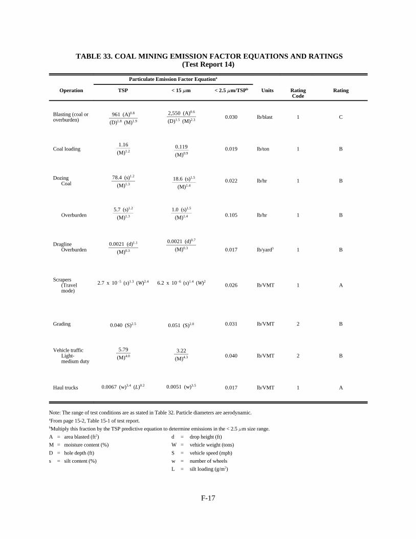
F-17
961 (A)0.8
(D)1.8 (M)1.9
0.119
(M)0.9
78.4 (s)1.2
(M)1.318.6 (s)1.5
(M)1.4
5.7 (s)1.2
(M)1.3
1.0 (s)1.5
(M)1.4
0.0021 (d)1.1
(M)0.3
0.0021 (d)0.7
(M)0.3
2.7 x 10&5 (s)1.3 (W)2.4 6.2 x 10&6 (s)1.4 (W)2.
0.040 (S)2.5 0.051 (S)2.0
5.79
(M)4.03.22
(M)4.3
0.0067 (w)3.4 (L)0.2 0.0051 (w)3.5
TABLE 33. COAL MINING EMISSION FACTOR EQUATIONS AND RATINGS(Test Report 14)
Particulate Emission Factor Equationa
Operation TSP < 15 FFm < 2.5 FFm/TSPb Units RatingCode
Rating
Blasting (coal oroverburden)
2,550 (A)0.6
(D)1.5 (M)2.30.030 lb/blast 1 C
Coal loading1.16
(M)1.2 0.019 lb/ton 1 B
DozingCoal 0.022 lb/hr 1 B
Overburden 0.105 lb/hr 1 B
DraglineOverburden 0.017 lb/yard3 1 B
Scrapers(Travelmode)
0.026 lb/VMT 1 A
Grading 0.031 lb/VMT 2 B
Vehicle trafficLight-medium duty
0.040 lb/VMT 2 B
Haul trucks 0.017 lb/VMT 1 A
Note: The range of test conditions are as stated in Table 32. Particle diameters are aerodynamic.aFrom page 15-2, Table 15-1 of test report.bMultiply this fraction by the TSP predictive equation to determine emissions in the < 2.5 Fm size range.
A = area blasted (ft2) d = drop height (ft)
M = moisture content (%) W = vehicle weight (tons)
D = hole depth (ft) S = vehicle speed (mph)
s = silt content (%) w = number of wheels
L = silt loading (g/m2)
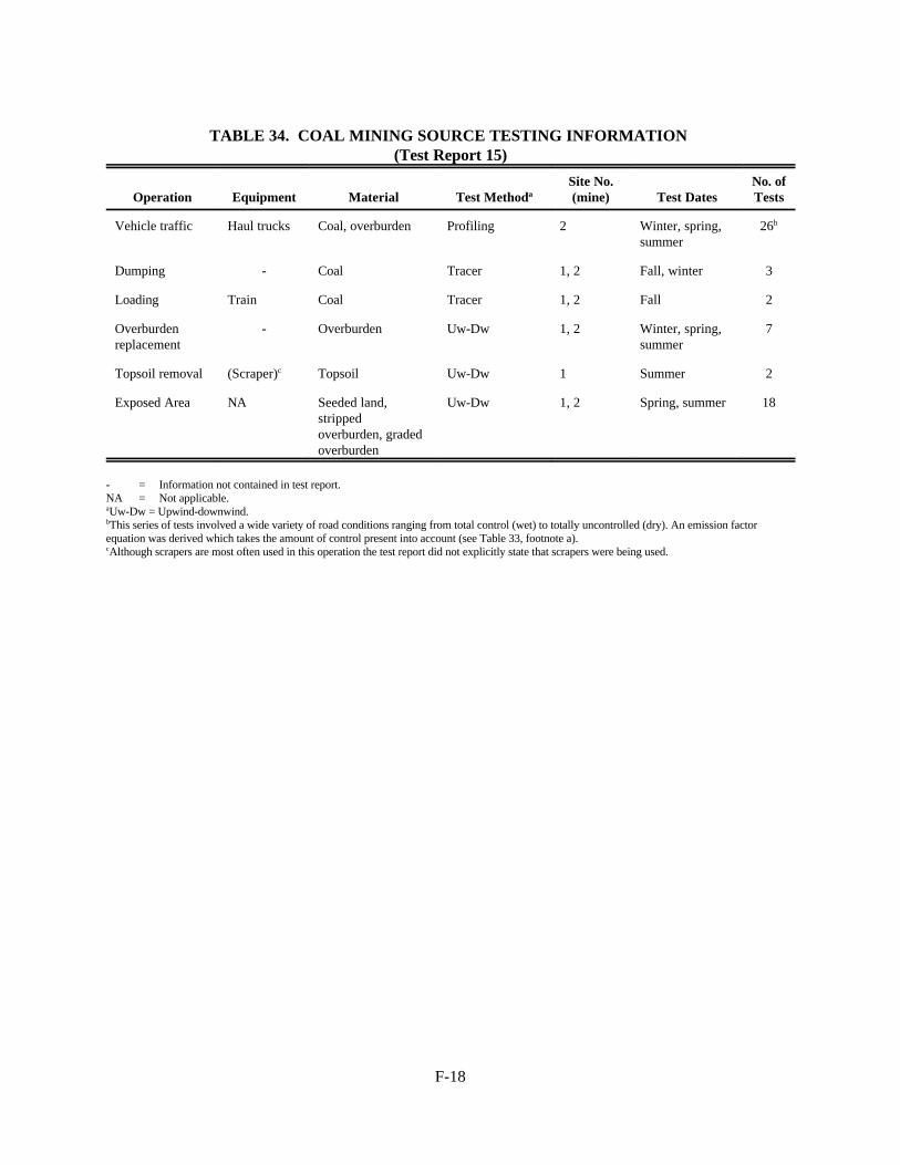
F-18
TABLE 34. COAL MINING SOURCE TESTING INFORMATION (Test Report 15)
Operation Equipment Material Test MethodaSite No.(mine) Test Dates
No. ofTests
Vehicle traffic Haul trucks Coal, overburden Profiling 2 Winter, spring,summer
26b
Dumping - Coal Tracer 1, 2 Fall, winter 3
Loading Train Coal Tracer 1, 2 Fall 2
Overburdenreplacement
- Overburden Uw-Dw 1, 2 Winter, spring,summer
7
Topsoil removal (Scraper)c Topsoil Uw-Dw 1 Summer 2
Exposed Area NA Seeded land,strippedoverburden, gradedoverburden
Uw-Dw 1, 2 Spring, summer 18
- = Information not contained in test report.NA = Not applicable.aUw-Dw = Upwind-downwind.bThis series of tests involved a wide variety of road conditions ranging from total control (wet) to totally uncontrolled (dry). An emission factorequation was derived which takes the amount of control present into account (see Table 33, footnote a).cAlthough scrapers are most often used in this operation the test report did not explicitly state that scrapers were being used.

F-19
Vd ' 1.51 (x)&0.588 (9)
The upwind-downwind sampling system consisted of 10 Hi-Vols of which two were placed upwind
and eight were placed at multiple downwind and crosswind distances. Wind direction and speed were
concurrently measured at an on-site station for all test periods. This sampling system meets the minimum
requirements set forth in Section 4.3. However, the emission factors are rated B because these operations
tested (overburden replacement, coal dumping, and top soil removal) were not described as to the
equipment employed (see Table 34).
The calculated TSP emission rates were modified with a depletion factor, as follows. A deposition
velocity was determined from dustfall bucket measurements:
where Vd = deposition velocity
x = distance downwind of source
This velocity was combined with stability class and wind speed to derive a depletion factor in terms
of distance downwind of a particulate source. The actual emission rate for an operation was then calculated
through division of the apparent emission rate (measured at a particular distance downwind) by the
appropriate depletion factor.
Table 35 gives the range of test conditions, emission factors, and applicable ratings for Test
Report 16. The rating codes refer to Table 4. These ratings overlook the particle size incompatibility
between the Hi-Vol measurements of particulate flux and the dustfall measurements of deposition velocity.
8.5 Western Surface Coal Mining and Processing
Since no emission factors are currently presented in AP-42 for coal mining. The predictive
emission factor equations presented in Table 49 are recommended for inclusion in AP-42 under a section
named “Western Surface Coal Mining.” Table 50 presents the single-valued emission factors for western
surface coal mining. It is recommended that for any source operation not covered by the equations in
Table 49, the highest rated single-valued factors from Table 50 be incorporated in AP-42.
All of the recommended factors may be applied to Eastern surface coal mining. However, each
should then be aerated one letter value (e.g., C to D).
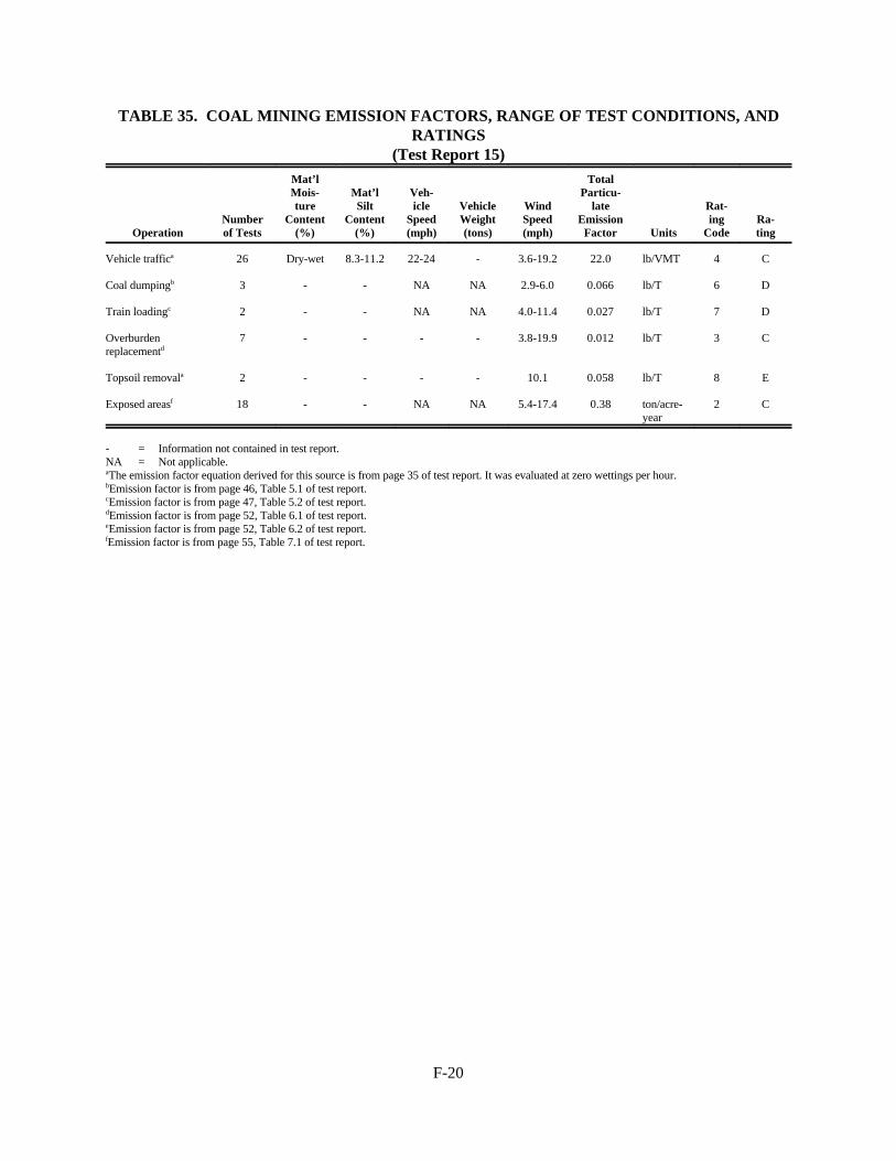
F-20
TABLE 35. COAL MINING EMISSION FACTORS, RANGE OF TEST CONDITIONS, ANDRATINGS
(Test Report 15)
OperationNumberof Tests
Mat’lMois-ture
Content(%)
Mat’lSilt
Content(%)
Veh-icle
Speed(mph)
VehicleWeight(tons)
WindSpeed(mph)
TotalParticu-
lateEmission
Factor Units
Rat-ing
CodeRa-ting
Vehicle traffica 26 Dry-wet 8.3-11.2 22-24 - 3.6-19.2 22.0 lb/VMT 4 C
Coal dumpingb 3 - - NA NA 2.9-6.0 0.066 lb/T 6 D
Train loadingc 2 - - NA NA 4.0-11.4 0.027 lb/T 7 D
Overburdenreplacementd
7 - - - - 3.8-19.9 0.012 lb/T 3 C
Topsoil removala 2 - - - - 10.1 0.058 lb/T 8 E
Exposed areasf 18 - - NA NA 5.4-17.4 0.38 ton/acre-year
2 C
- = Information not contained in test report.NA = Not applicable.aThe emission factor equation derived for this source is from page 35 of test report. It was evaluated at zero wettings per hour.bEmission factor is from page 46, Table 5.1 of test report.cEmission factor is from page 47, Table 5.2 of test report.dEmission factor is from page 52, Table 6.1 of test report.eEmission factor is from page 52, Table 6.2 of test report.fEmission factor is from page 55, Table 7.1 of test report.

F-21
0.119
(M)0.9
78.4 (s)1.2
(M)1.318.6 (s)1.5
(M)1.4
5.7 (s)1.2
(M)1.318.6 (s)1.5
(M)1.4
0.0021 (d)1.1
(M)0.31.0 (s)1.5
(M)1.4
2.7 x 10&5 (s)1.3 (W)2.4 6.2 x 10&6 (s)1.4 (W)2.5
0.040 (S)2.5
0.051 (S)2.0
5.79
(M)4.0
3.72
(M)4.3
0.0067 (w)3.4 (L)0.2 0.0051 (w)3.5
lb(acre)(hr)
TABLE 49. WESTERN SURFACE COAL MINING PREDICTIVE EMISSION FACTOREQUATIONS
(Test Reports 5 and 14)
Particulate Emission Factor Equation
Operation Material TSP < 15 FFm< 2.5
FFm/TSPa UnitsTestRe-port
Rating
BlastingCoal oroverburden
961 (A)0.8
(D)1.8 (M)1.9
2,550 (A)0.6
(D)1.5 (M)2.30.030 lb/blast 14 C
Truck loading Coal1.16
(M)1.2 0.019 lb/ton 14 B
Dozing Coal 0.022 lb/hr 14 B
Overburden 0.105 lb/hr 14 B
Dragline Overburden 0.017 lb/yard3 14 B
Scrapers (travelmode)
0.026 lb/VMT 14 A
Grading 0.031 lb/VMT 14 B
Vehicle traffic(light-mediumduty)
0.040 lb/VMT 14 B
Haul trucks 0.017 lb/VMT 14 A
Storage pile(Winderosion andmainten-ance
Coal 1.6 u - - 5 Cb
- = Unable to be determined from information contained in test report.aMultiply this fraction by the TSP predictive equation to determine emissions in the < 2.5 Fm size range.bRating applicable to Mine Types A, B, and D (see p 61).A = area blasted (ft2) d = drop height (ft)M = moisture content (%) W = vehicle weight (tons)D = hole depth (ft) S = vehicle speed (mph)s = silt content (%) w = number of wheelsF = wind speed (m/sec) L = silt loading (g/m2)
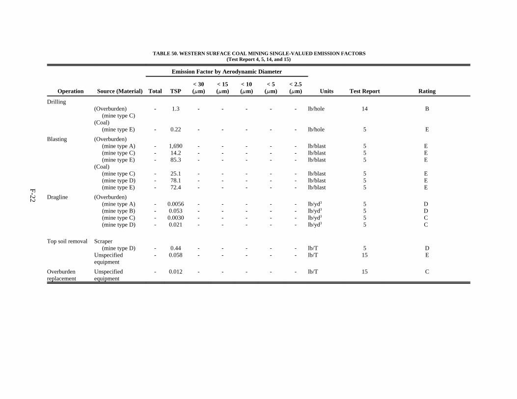
F-22
TABLE 50. WESTERN SURFACE COAL MINING SINGLE-VALUED EMISSION FACTORS(Test Report 4, 5, 14, and 15)
Emission Factor by Aerodynamic Diameter
Operation Source (Material) Total TSP< 30(FFm)
< 15(FFm)
< 10(FFm)
< 5(FFm)
< 2.5(FFm) Units Test Report Rating
Drilling(Overburden)
(mine type C)(Coal)
(mine type E)
-
-
1.3
0.22
-
-
-
-
-
-
-
-
-
-
lb/hole
lb/hole
14
5
B
E
Blasting (Overburden)(mine type A)(mine type C)(mine type E)
(Coal)(mine type C)(mine type D)(mine type E)
---
---
1,69014.285.3
25.178.172.4
---
---
---
---
---
---
---
---
---
---
lb/blastlb/blastlb/blast
lb/blastlb/blastlb/blast
555
555
E*E*E*
E*E*E*
Dragline (Overburden)(mine type A)(mine type B)(mine type C)(mine type D)
----
0.00560.0530.00300.021
----
----
----
----
----
lb/yd3
lb/yd3
lb/yd3
lb/yd3
5555
D*D*C*C*
Top soil removal Scraper(mine type D)
Unspecifiedequipment
--
0.440.058
--
--
--
--
--
lb/Tlb/T
515
DE
Overburdenreplacement
Unspecifiedequipment
- 0.012 - - - - - lb/T 15 C

F-23
TABLE 50. WESTERN SURFACE COAL MINING SINGLE-VALUED EMISSION FACTORS(Test Report 4, 5, 14, and 15) (cont.)
Emission Factor by Aerodynamic Diameter
Operation Source (Material) Total TSP< 30(FFm)
< 15(FFm)
< 10(FFm)
< 5(FFm)
< 2.5(FFm) Units Test Report Rating
Batch-drop Dumping via truck(Overburden-bottom)
(mine type E)(Coal-end)
(mine type E)(Material notspecified-bottom)
(mine type A)(mine type B)(mine type C)(mine type D)
Dumping viascraper (top soil)
(mine type D)Dumping viaunspecifiedequipment orprocess(Coal)(Fly-ash)
(mine type A)Front-endloader/truck(Materialunspecified)
(mine type D)Power shovel/truck(Overburden)
(mine type E)
-
-
----
-
-
-
-
-
0.002
0.007
0.0140.0200.0050.027
0.04
0.066
3.9
0.12
0.037
-
-
----
-
-
-
-
-
-
-
----
-
-
-
-
-
-
-
----
-
-
-
-
-
-
-
----
-
-
-
-
-
-
-
----
-
-
-
-
-
lb/T
lb/T
lb/Tlb/Tlb/Tlb/T
lb/T
lb/T
lb/hr
lb/T
lb/T
5
5
5555
5
15
5
5
5
E
E
DEEE
C
D
E*
E*
C
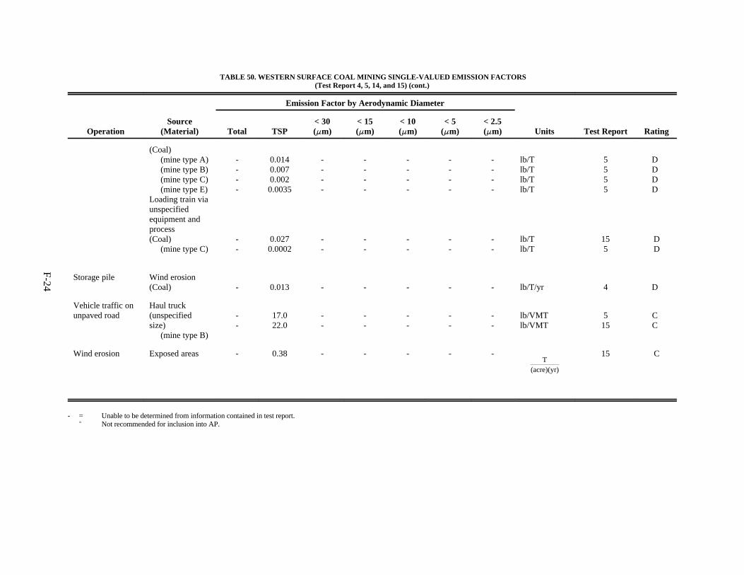
F-24
T(acre)(yr)
TABLE 50. WESTERN SURFACE COAL MINING SINGLE-VALUED EMISSION FACTORS(Test Report 4, 5, 14, and 15) (cont.)
Emission Factor by Aerodynamic Diameter
OperationSource
(Material) Total TSP< 30(FFm)
< 15(FFm)
< 10(FFm)
< 5(FFm)
< 2.5(FFm) Units Test Report Rating
(Coal)(mine type A)(mine type B)(mine type C)(mine type E)
Loading train viaunspecifiedequipment andprocess(Coal)
(mine type C)
----
--
0.0140.0070.0020.0035
0.0270.0002
----
--
----
--
----
--
----
--
----
--
lb/Tlb/Tlb/Tlb/T
lb/Tlb/T
5555
155
D*D*D*D*
DD
Storage pile Wind erosion(Coal) - 0.013 - - - - - lb/T/yr 4 D*
Vehicle traffic onunpaved road
Haul truck(unspecifiedsize)
(mine type B)
--
17.022.0
--
--
--
--
--
lb/VMTlb/VMT
515
C*C*
Wind erosion Exposed areas - 0.38 - - - - - 15 C
- = Unable to be determined from information contained in test report.* = Not recommended for inclusion into AP.

F-25
F.2 Section 8 of EPA report "Improved Emission Factors for Fugitive Dust from Western Surface Coal Mining Sources--Volume I - Sampling
Methodology and Test Results
SECTION 8
RESULTS FOR SOURCES TESTED BY UPWIND-DOWNWIND SAMPLING
SUMMARY OF TESTS PERFORMED
Five different sources were tested by the upwind-downwind method--coal loading, dozers,
draglines, haul roads, and scrapers. However, haul roads and scrapers were tested by upwind-downwind
sampling only as part of the comparability study, with the exception of six additional upwind-downwind
haul road tests during the winter sampling period. Test conditions, net concentrations, and calculated
emission rates for the comparability tests were presented in Section 6. Test conditions and emission rates
for haul road tests are repeated here for easier comparison with winter haul road tests, but scraper data are
not shown again. Haul roads were tested by the upwind-downwind method during the winter when limited
operations and poor choices for sampling locations precluded sampling of dozers or draglines, the two
primary choices.
A total of 87 successful upwind-downwind tests were conducted at the three mines/four visits.
They were distributed by source and by mine as follows:
Number of tests
Source Mine 1 Mine 2 Mine 1W Mine 3
Coal loading 2 8 15
Dozer, overburden 4 7 4
Dozer, coal 4 3 5
Draglines 6 5 8
Haul roads 5 6
Scrapers 5

F-26
Test conditions for the coal loading tests are summarized in Table 8-1. Correction factors for this
source may be difficult to develop: bucket capacities and silt contents did not vary significantly during the
tests, nor did drop distances (not shown in the table). One variable not included in the table was type of
coal loading equipment. At the first two mines, shovels were used; at the third mine, front-end loaders were
used.
Test conditions for dozers are summarized in Tables 8-2 and 8-3 for dozers working overburden
and coal, respectively. These two source categories exhibited a wide range of operating and soil
characteristics in their tests--speed varied from 2 to 10 mph, silt contents from 3.8 to 15.1 percent, and
moisture contents from 2.2 to 22 percent. This indicates a good potential for correction factors. Also, there
is a possibility of producing a single emission factor for the two dozer operations.
Dragline test conditions are shown in Table 8-4. Bucket sizes for the different tests were all nearly
the same, but large differences in drop distances (5 to 100 ft), silt contents (4.6 to 14 percent), and moisture
contents (0.2 to 16.3 percent) were obtained. One dragline variable used in the preliminary data analysis for
the statistical plan, operator skill, was not included in Table 8-4 because it was judged to be too subjective
and of little value as a correction factor for predicting emissions from draglines. Also, it was not found to
be a significant variable in the preliminary data analysis.
Test conditions for haul roads tested by upwind-downwind sampling are summarized in Table 8-5.
Most of the tests for this source were done by exposure profiling, so this subset of tests was not analyzed
separately to develop another emission factor. Instead, the calculated emission rates and test conditions for
these tests were combined with the exposure profiling test data in the data analysis and emission factor
development phase.
RESULTS
The apparent TSP emission rates calculated from the concentrations at each hi-vol sampler are
shown in Tables 8-6 through 8-10 for coal loading, dozers (overburden), dozers (coal), draglines, and haul
roads, respectively. These reported emission rates have not been adjusted for any potential correction
factors. The individual emission rates are shown as a function of source sampler distances in these tables.
Distance is an important factor in the evaluation of deposition.

F-27
TABLE 8-1. TEST CONDITIONS FOR COAL LOADING
Source Characteristics Soil Properties Meteorological Conditions
Test Date Start Time
SamplingDuration,Minutes
No. ofTrucks
BucketCapacity,
Yd3 Silt, %Moisture,
% Temp., EEFWind
Speed, m/s Stab Class
Mine 112
8/11/798/11/79
12:3513:45
4339
103
1717
Nodata
2222
8791
1.01.0
AA
Mine 212345678
10/16/7910/16/7910/16/7910/16/7910/18/7910/18/7910/18/7910/30/79
9:4512:4516:0017:009:40
12:5015:3016:00
7280453042403635
44433225
1414141414141416
Nodata
3838383838383838
4655565650576038
4.34.32.92.62.14.84.95.0
CCCCCDDC
Mine 3123456789101112131415
7/26/807/26/807/26/807/30/807/30/807/30/808/05/808/07/808/07/808/07/808/07/808/12/808/12/808/12/808/12/80
8:349:26
10:2710:3511:5012:5810:159:17
10:0212:0012:488:42
10:0310:4211:30
354424235265543446284722181322
2324
108232344233
161616161616161616161616161616
3.63.63.64.24.24.23.94.04.04.04.03.73.73.73.7
11.911.911.918.018.018.012.211.111.111.111.16.66.66.66.6
74808294959593828310010079898989
1.71.01.01.11.12.91.31.01.31.21.92.01.91.82.5
CAAAABBCDBACCCD
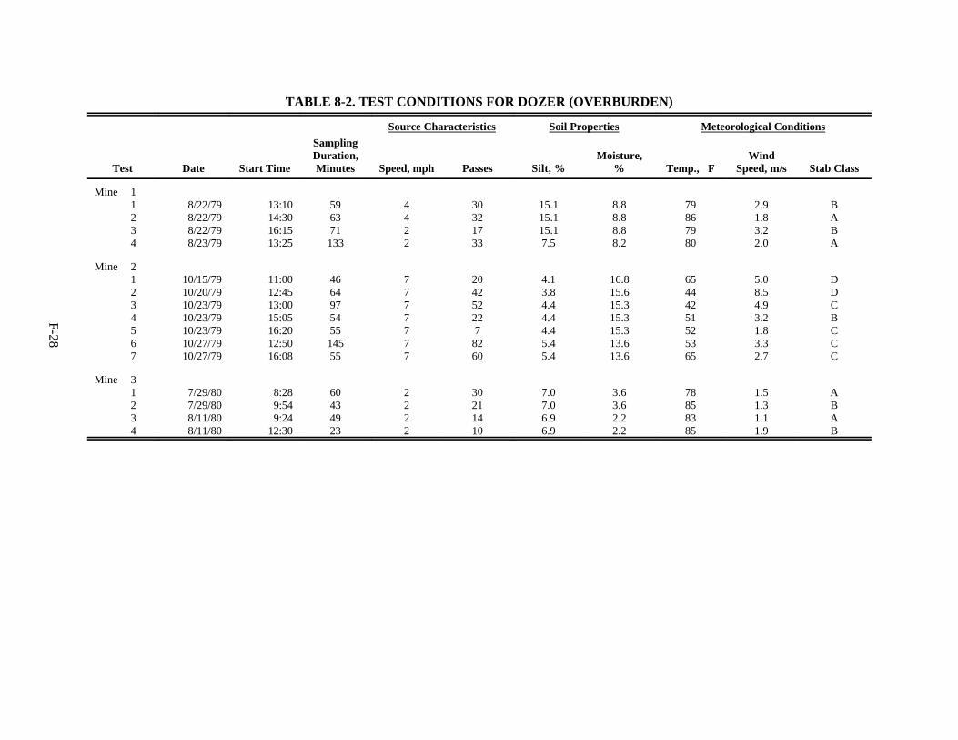
F-28
TABLE 8-2. TEST CONDITIONS FOR DOZER (OVERBURDEN)
Source Characteristics Soil Properties Meteorological Conditions
Test Date Start Time
SamplingDuration,Minutes Speed, mph Passes Silt, %
Moisture,% Temp., EEF
WindSpeed, m/s Stab Class
Mine 11234
8/22/798/22/798/22/798/23/79
13:1014:3016:1513:25
596371133
4422
30321733
15.115.115.17.5
8.88.88.88.2
79867980
2.91.83.22.0
BABA
Mine 21234567
10/15/7910/20/7910/23/7910/23/7910/23/7910/27/7910/27/79
11:0012:4513:0015:0516:2012:5016:08
466497545514555
7777777
204252227
8260
4.13.84.44.44.45.45.4
16.815.615.315.315.313.613.6
65444251525365
5.08.54.93.21.83.32.7
DDCBCCC
Mine 31234
7/29/807/29/808/11/808/11/80
8:289:549:24
12:30
60434923
2222
30211410
7.07.06.96.9
3.63.62.22.2
78858385
1.51.31.11.9
ABAB
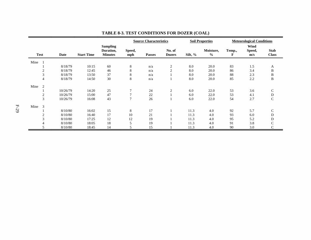
F-29
TABLE 8-3. TEST CONDITIONS FOR DOZER (COAL)
Source Characteristics Soil Properties Meteorological Conditions
Test Date Start Time
SamplingDuration,Minutes
Speed,mph Passes
No. ofDozers Silt, %
Moisture,%
Temp.,EEF
WindSpeed,
m/sStabClass
Mine 11234
8/18/798/18/798/18/798/18/79
10:1512:4513:5014:50
60463730
8888
n/an/an/an/a
2211
8.08.08.08.0
20.020.020.020.0
83868885
1.53.42.32.2
ABBB
Mine 2123
10/26/7910/26/7910/26/79
14:2015:0016:08
254743
777
242226
211
6.06.06.0
22.022.022.0
535354
3.64.12.7
CDC
Mine 312345
8/10/808/10/808/10/808/10/808/10/80
16:0216:4017:2518:0518:45
1517121814
8101255
1721191915
11111
11.311.311.311.311.3
4.04.04.04.04.0
9293959190
5.76.05.23.83.0
CDDCC

F-30
TABLE 8-4. TEST CONDITIONS FOR DRAGLINES
Source Characteristics Soil Properties Meteorological Conditions
Test Date Start Time
SamplingDuration,Minutes Buckets
BucketCapacity,
Yd3
DropDist.,
Ft. Silt, %Moisture,
%Temp.,EEF
WindSpeed,
m/sStabClass
Mine 1123456
8/08/798/08/798/08/798/17/798/17/798/17/79
11:1514:0916:4011:0014:4016:00
496260444931
32464454495
606060606060
103220283082
6.46.46.46.46.46.4
8.48.48.48.48.48.4
788388848684
2.43.13.92.01.01.8
BBCAAA
Mine 212345
10/13/7910/13/7910/13/7910/21/7910/24/79
12:1514:2816:0012:4814:45
6872745283
637166466
3232323232
40405
1030
11.411.411.412.65.0
15.615.615.616.314.9
4752533854
4.74.13.63.92.7
DCCDC
Mine 312345678
7/31/807/31/807/31/807/31/808/02/808/02/808/02/808/02/80
10:1911:3512:4013:2810:3011:3512:3413:45
4153355529402655
3037402222241823
5555555565656565
100601003010202525
14.014.014.04.65.05.05.05.0
2.72.72.71.20.20.20.20.2
8593949688888890
1.01.92.22.16.27.44.13.6
AABBDDCC
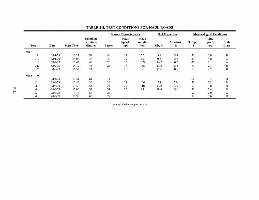
F-31
TABLE 8-5. TEST CONDITIONS FOR HAUL ROADS
Source Characteristics Soil Properties Meteorological Conditions
Test Date Start Time
SamplingDuration,Minutes Passes
MeanSpeed,mph
MeanWeight,
ton Silt, %Moisture,
%Temp.,EEF
WindSpeed,
m/sStabClass
Mine 1J9J10J12J20J21
8/01/798/01/798/02/798/09/798/09/79
10:2114:0210:4714:1016:52
5947494621
4443202313
1919151715
7266109138121
9.49.414.211.611.6
3.42.26.88.58.5
8389817377
3.84.81.12.12.2
BCABB
Mine 1W123456
12/04/7912/08/7912/08/7912/08/7912/09/7912/09/79
10:5412:4013:5015:009:15
10:30
643854525563
142824312522
242020
10611895
15.9a
13.818.0
5.0a
4.95.1
645356565259
5.76.25.85.42.05.0
DDDDCD
aAverage of other samples this day.

F-32
TABLE 8-6. APPARENT EMISSION RATES FOR COAL LOADINGHigh Volume (30 FFm)
Apparent Emission Rates at Specified Distances, lb/ton
Test No. First Second Third Fourth Distances from Source, m
Mine 112
0.0060.005
0.0050.004
0.0050.010
0.0050.008
0.0060.010
0.0080.017
0.0100.016
0.0100.031
2520
5045
8075
Mine 212345678
0.0300.0430.0140.0130.0050.0220.0300.005
0.0570.0890.0230.0180.0070.0250.0080.004
0.0500.0710.0190.0130.0070.0390.0110.005
0.0480.1210.0170.0120.0080.0120.0180.004
0.0340.0670.0110.0100.0150.0210.0380.005
0.043a
0.0170.0160.004
0.009
0.081a
0.0450.0260.0130.0130.0120.010
0.045a
0.0020.0120.0170.017
0.010
0.0130.0330.027
3465578030101030
65968210562282860
1311621832061016262110 199
170170
Mine 3123456789
101112131415
0.1280.1150.0600.0050.0060.008
0.0410.0420.1940.0410.0390.3640.1650.177
0.1130.0490.067
0.0050.0140.0050.0510.0470.1000.0290.0340.8420.2820.161
0.1680.0080.0550.0160.0070.0100.0260.0690.0590.2000.1300.0490.9120.2910.131
0.0380.0610.0380.0110.0070.016
a
0.0700.0640.1330.0450.0511.2710.3560.128
0.0720.0430.0350.0120.0130.0210.041
0.0880.0530.0560.0190.0140.0150.0360.0790.0660.2140.1910.0361.2180.3520.265
0.0360.057
0.0560.1040.0700.2220.1340.0771.2140.5070.267
0.0150.0430.0510.009
0.017
0.0250.0550.0420.0100.0190.029
1113129121616106045452935353535
1325856242727209075654965656262
1489694313434351301151058995959292
166150148455050
aInterference from truck trafic.

F-33
TABLE 8-7. APPARENT EMISSION RATES FOR DOZER (OVERBURDEN)High Volume (30 FFm)
Apparent Emission Rates at Specified Distances, lb/h
Test No. First Second Third Fourth Distance from Source, m
Mine 11234
14.312.02.53.4
18.213.02.65.5
11.617.02.34.9
9.017.90.81.3
7.87.93.22.3
10.322.21.80.6
10.515.7
aa
a
8.92.48.1
4.58.21.513.1
15202525
44495452
78838878
180185190138
Mine 21234567
0.82.11.83.0
0.81.0
0.30.62.22.91.60.71.5
2.0a
2.30.84.80.80.7
0.60.71.80.00.00.41.3
6.1
2.11.93.6
3.03.70.08.61.21.5
2.43.50.017.3
3.5
1.83.50.019.8
5.36.33.217.62.40.0
2.71.0
252025258
31
564658582366
811001001005390
151162162162103146
Mine 31234
4.52.521.025.9
5.24.814.9
4.65.018.020.1
5.54.317.815.9
8.05.0
3.86.414.417.7
7.04.916.723.9
8.85.0
4.86.3
25202543
45404159
75706381
115110
aUsed as upwind concentration.

F-34
TABLE 8-8. APPARENT EMISSION RATES FOR DOZER (COAL)High-Volume (30 FFm)
Apparent Emission Rates at Specified Distances, lb/h
Test No. First Second Third Fourth Distance from Source, m
Mine 11234
13.447.18.311.9
16.734.938.522.0
12.140.912.116.5
15.434.312.525.0
20.123.119.030.8
16.834.8
bb
14.150.831.218.4
23.537.945.046.8
20.4a
11.624.3
125125125125
155155155155
193193193193
292292292292
Mine 2123
9.73.01.6
8.05.82.5
10.45.23.8
8.66.63.4
6.48.44.2
11.54.61.0
13.49.54.4
304040
426767
537878
Mine 312345
281298300255160
234453255152
284217533324243
303153427368193
229164540306239
340217540414245
283250526366300
300242670293261
3030303030
6060606060
9191919191
133133133133133
aLess than upwind concentration.bUsed as upwind concentration.
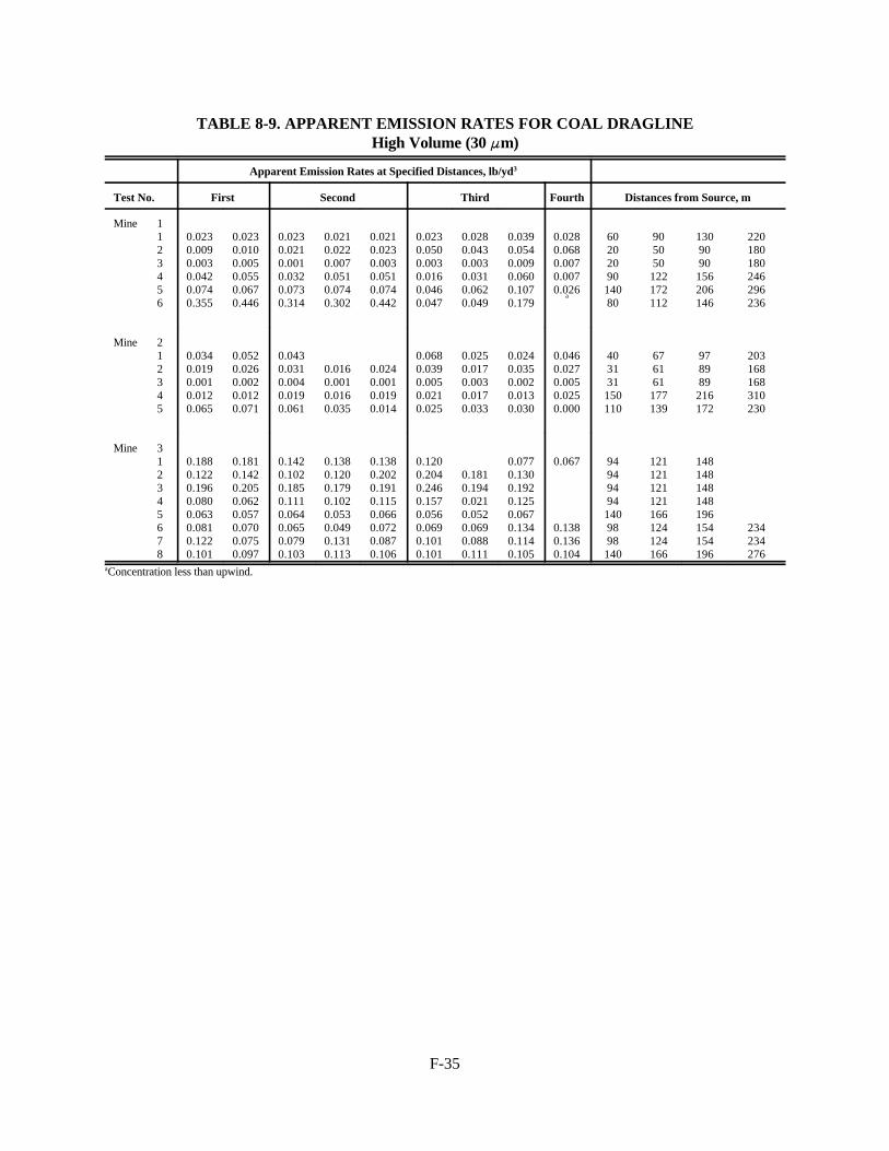
F-35
TABLE 8-9. APPARENT EMISSION RATES FOR COAL DRAGLINEHigh Volume (30 FFm)
Apparent Emission Rates at Specified Distances, lb/yd3
Test No. First Second Third Fourth Distances from Source, m
Mine 1123456
0.0230.0090.0030.0420.0740.355
0.0230.0100.0050.0550.0670.446
0.0230.0210.0010.0320.0730.314
0.0210.0220.0070.0510.0740.302
0.0210.0230.0030.0510.0740.442
0.0230.0500.0030.0160.0460.047
0.0280.0430.0030.0310.0620.049
0.0390.0540.0090.0600.1070.179
0.0280.0680.0070.0070.026
a
6020209014080
905050122172112
1309090156206146
220180180246296236
Mine 212345
0.0340.0190.0010.0120.065
0.0520.0260.0020.0120.071
0.0430.0310.0040.0190.061
0.0160.0010.0160.035
0.0240.0010.0190.014
0.0680.0390.0050.0210.025
0.0250.0170.0030.0170.033
0.0240.0350.0020.0130.030
0.0460.0270.0050.0250.000
403131150110
676161177139
978989216172
203168168310230
Mine 312345678
0.1880.1220.1960.0800.0630.0810.1220.101
0.1810.1420.2050.0620.0570.0700.0750.097
0.1420.1020.1850.1110.0640.0650.0790.103
0.1380.1200.1790.1020.0530.0490.1310.113
0.1380.2020.1910.1150.0660.0720.0870.106
0.1200.2040.2460.1570.0560.0690.1010.101
0.1810.1940.0210.0520.0690.0880.111
0.0770.1300.1920.1250.0670.1340.1140.105
0.067
0.1380.1360.104
949494941409898140
121121121121166124124166
148148148148196154154196
234234276
aConcentration less than upwind.
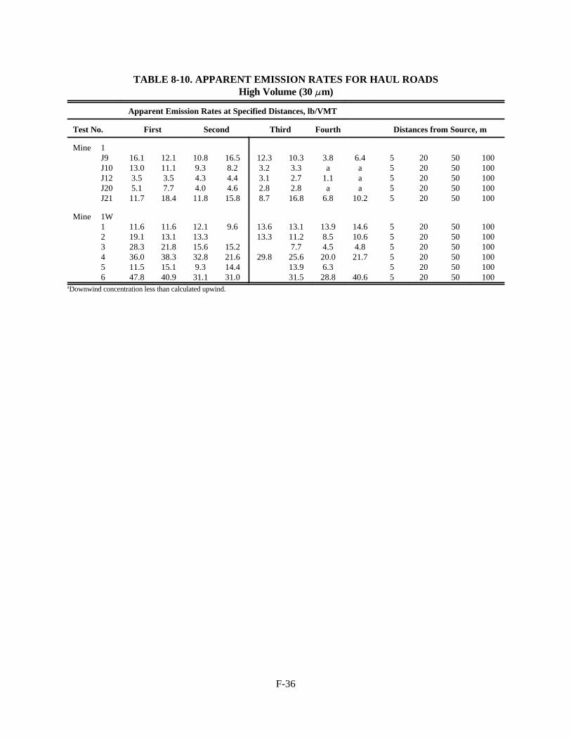
F-36
TABLE 8-10. APPARENT EMISSION RATES FOR HAUL ROADSHigh Volume (30 FFm)
Apparent Emission Rates at Specified Distances, lb/VMT
Test No. First Second Third Fourth Distances from Source, m
Mine 1J9J10J12J20J21
16.113.03.55.111.7
12.111.13.57.718.4
10.89.34.34.011.8
16.58.24.44.615.8
12.33.23.12.88.7
10.33.32.72.816.8
3.8a
1.1a
6.8
6.4aaa
10.2
55555
2020202020
5050505050
100100100100100
Mine 1W123456
11.619.128.336.011.547.8
11.613.121.838.315.140.9
12.113.315.632.89.331.1
9.6
15.221.614.431.0
13.613.3
29.8
13.111.27.725.613.931.5
13.98.54.520.06.328.8
14.610.64.821.7
40.6
555555
202020202020
505050505050
100100100100100100
aDownwind concentration less than calculated upwind.

F-37
When the samples were evaluated for deposition as described in Section 5, only 21 out of the 87
upwind-downwind samples (including scrapers) demonstrated distinct fallout over the three or four
distances. The percentage of tests showing fallout was much higher for sources sampled as line sources
than for sources sampled as point sources: 13 out of 25 (52 percent) for line sources compared to 8 out of
62 (12.g percent) for point sources.
It was concluded that some problem exists with the point source dispersion equation because its
results rarely indicate deposition, although the same type and size distribution of emissions are involved as
with the line source dispersion equation. The sensitivity of calculated emission rates to several inputs to the
point source equation (such as initial plume width, initial horizontal dispersion, distance from plume
centerline, and stability class) were examined, but no single input parameter could be found that would
change the emission data by distance to show deposition.
The single-value TSP emission rates for each test determined from the multiple emission rate values
are summarized in Table 8-11. The means and standard deviations for these tests are shown below:
Source No. Tests Units Mean Std Dev Range
Coal loading 25 lb/ton 0.105 0.220 0.0069-1.09
Dozer, overburden 15 lb/h 6.8 6.9 0.9-20.7
Dozer, coal 12 1b/h 134.3 155.6 3.0-439
Dragline 19 lb/yd3 0.088 0.093 0.003-0.400
Haul road 11 lb/VMT 17.4 10.9 3.6-37.2
Scraper 5 1b/VMT 18.1 11.4 5.7-35.6
It should be emphasized that the mean values reported here are not emission factors; they do not have any
consideration of correction factors included in them.
Emission rates for coal loading varied over a wide range, from 0.0069 to 1.09 lb/ton. Rates at the
third mine averaged an order of magnitude higher than at the first two mines. Since a front-end loader was
used at the third mine and shovels at the first two, the wide differences in average emission rates may
indicate that separate emission factors are required for these two types of coal loading.

F-38
TABLE 8-11. EMISSION RATES FOR UPWIND-DOWNWIND TESTS
Coal Loading Dozer, Overburden Dozer, Coal Dragline Haul Road/Scraper
Test No.
EmissionRate,lb/ton Test No.
EmissionRate,lb/h Test No.
EmissionRate,lb/h Test No.
EmissionRate,lb/yd3 Test No.
EmissionRate,
lb/VMT
Mine 112
Mine 212345678
Mine 3123456789101112131415
0.00690.0100
0.0440.0680.01470.01340.00990.02280.02060.0065
0.1200.0820.0510.01050.00870.01400.0350.0620.0580.1930.0950.0421.09
0.3580.188
Mine 11234
Mine 21234567
Mine 31234
16.212.62.63.0
0.91.82.61.39.21.01.0
5.45.218.020.7
Mine 11234
Mine 2123
Mine 312345
16.140.119.021.3
9.16.23.0
289222439323224
Mine 1123456
Mine 212345
Mine 312345678
0.0240.0290.0040.0480.0700.400
0.0420.0260.0030.0160.068
0.1840.1330.1920.0990.0600.1040.105
Haul RoadMine 1
J9J10J12J20J21
Mine 1W123456
ScraperMine 1
J1J2J3J4J5
14.112.03.66.415.0
12.916.125.037.212.836.0
10.618.635.65.720.0
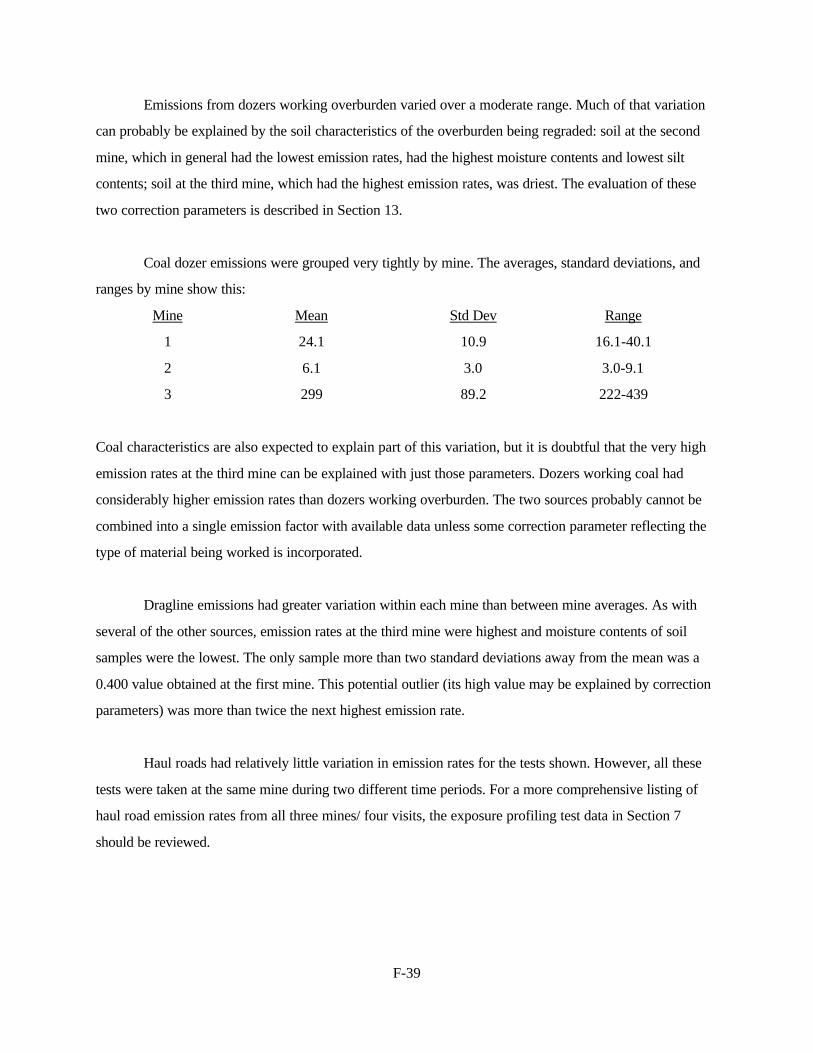
F-39
Emissions from dozers working overburden varied over a moderate range. Much of that variation
can probably be explained by the soil characteristics of the overburden being regraded: soil at the second
mine, which in general had the lowest emission rates, had the highest moisture contents and lowest silt
contents; soil at the third mine, which had the highest emission rates, was driest. The evaluation of these
two correction parameters is described in Section 13.
Coal dozer emissions were grouped very tightly by mine. The averages, standard deviations, and
ranges by mine show this:
Mine Mean Std Dev Range
1 24.1 10.9 16.1-40.1
2 6.1 3.0 3.0-9.1
3 299 89.2 222-439
Coal characteristics are also expected to explain part of this variation, but it is doubtful that the very high
emission rates at the third mine can be explained with just those parameters. Dozers working coal had
considerably higher emission rates than dozers working overburden. The two sources probably cannot be
combined into a single emission factor with available data unless some correction parameter reflecting the
type of material being worked is incorporated.
Dragline emissions had greater variation within each mine than between mine averages. As with
several of the other sources, emission rates at the third mine were highest and moisture contents of soil
samples were the lowest. The only sample more than two standard deviations away from the mean was a
0.400 value obtained at the first mine. This potential outlier (its high value may be explained by correction
parameters) was more than twice the next highest emission rate.
Haul roads had relatively little variation in emission rates for the tests shown. However, all these
tests were taken at the same mine during two different time periods. For a more comprehensive listing of
haul road emission rates from all three mines/ four visits, the exposure profiling test data in Section 7
should be reviewed.

F-40
Average IP and FP emission rates for each test, along with IP emission rates calculated from each
sampler, are presented by source in Tables 8-12 through 8-16. The values could be averaged without first
considering deposition because dichotomous samplers were only located at the first two distances from the
source (leaving only about a 30 m distance in which measurable deposition could occur) and because
smaller particles do not have significant deposition. Although the IP data from the upwind-downwind tests
have a large amount of scatter, no reduction in emission rates with distance is evident.
The average ratios of IP and FP to TSP emission rates are:
Avg. Ratio of IP to Avg. Ratio of FP to
Source TSP Emission Rates TSP Emission Rates
Coal loading 0.30 0.030
Dozer, overburden 0.86 0.196
Dozer, coal 0.49 0.031
Dragline 0.32 0.032
Haul road 0.42 0.024
These values are different than the average ratios of net concentrations because of the effect of deposition
on calculation of the single-value TSP emission rates.
The overburden dozer IP/TSP ratios are much higher than for other sources because five of the 15
tests had IP concentrations much higher than TSP concentrations. When the IP concentration exceeds the
TSP concentration, correction of the IP value to 15 Fm size from the actual (wind speed dependent) cut
point cannot be performed by the method described on Page 5-36. For such cases in Table 8-13 (and Table
8-14 through 8-16), the uncorrected IP values were reported along with their estimated cut points. If the
five tests with uncorrected IP data were eliminated, the average IP/TSP ratio would be 0.28, much closer to
that of the other sources. No explanation was found for the high IP concentrations compared to TSP
concentrations for overburden dozers.
For all sources except overburden dozers, the IP and FP emission rate variabilities (as measured by
the relative standard deviation) were about the same as TSP emission rate variabilities. Due to the four high
dichotomous sample values, the IP and FP emission rates for overburden dozers had about twice the
relative standard deviation as the TSP emission rates.

F-41
TABLE 8-12. EMISSION RATES FOR COAL LOADINGDichotomous (15 FFm, 2.5 FFm)
Apparent IP Emission Rates at SpecifiedDistances, lb/ton
Test No. First Second
Avg. IPEmission
Rate, lb/ton
Avg. FPEmission
Rate, lb/tonDistances from
Source, m
Mine 1
1 0.002 0.001 0.002 0.001 0.002 0.002 0.0001 25 50
2 0.001 0.001 0.002 0.007 0.006 0.003 0.0002 20 45
Mine 2
1 0.005 0.006 0.002 0.005 0.005 0.0002 34 65
2 0.013 0.050 0.018 0.009 0.022 0.0008 65 96
3 0.003 0.002 0.005 0.003 0.003 0.0001 57 82
4 0.002 0.008 0.005 0.005 0.005 0.0018 80 105
5 0.001 0.004 0.002 0.008 0.004 0.0007 30 62
6 0.005 0.011 0.039 0.014 0.017 0.0029 10 28
7 0.013 0.001 0.005 0.011 0.008 0.0008 10 28
8 0.004 0.003 0.005 0.004 0.0002 30 60
Mine 3
1 0.112 0.035 0.023 0.006 0.004 0.044 0.0038 111 132
2 0.011 0.005 0.008 0.0005 31 58
3 0.003 0.008 0.039 0.016 0.0022 29 56
4 0.001 0.001 0.004 0.001 0.002 0.0002 12 24
5 0.001 0.001 0.001 0.003 0.001 0.0001 16 27
6 0.002 0.009 0.011 0.003 0.006 0.0001 16 27
7 0.002 0.011 0.012 0.008 0.0012 10 20
8 0.011 0.000 0.018 0.020 0.012 0.0012 60 90
9 0.012 0.012 0.021 0.013 0.014 0.0005 45 75
10 0.051 0.029 0.040 0.036 0.038 0.0033 45 65
11 0.003 0.011 0.056 0.009 0.020 0.0005 29 49
12 0.012 0.006 0.015 0.010 0.011 0.0021 35 65
13 0.575 0.182 0.404 0.352 0.378 0.0054 35 65
14 0.116 0.093 0.152 0.122 0.121 0.0035 35 62
15 No dichotomous data for test
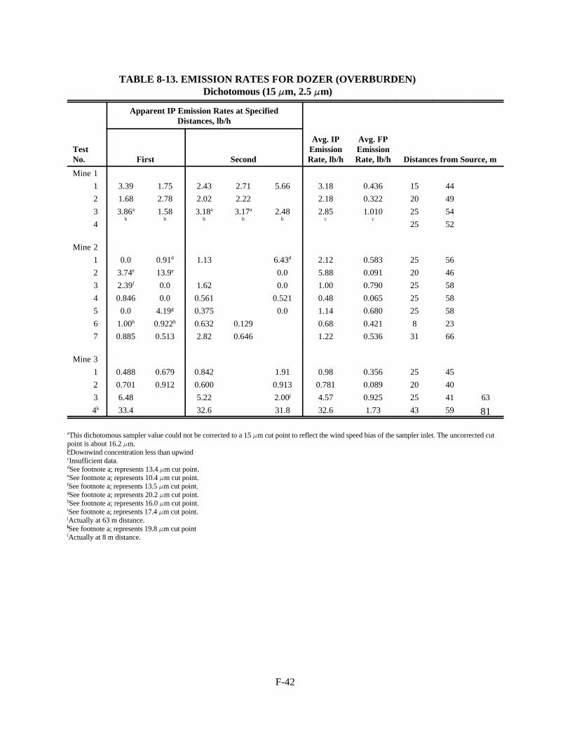
F-42
TABLE 8-13. EMISSION RATES FOR DOZER (OVERBURDEN)Dichotomous (15 FFm, 2.5 FFm)
Apparent IP Emission Rates at SpecifiedDistances, lb/h
TestNo. First Second
Avg. IPEmissionRate, lb/h
Avg. FPEmissionRate, lb/h Distances from Source, m
Mine 1
1 3.39 1.75 2.43 2.71 5.66 3.18 0.436 15 44
2 1.68 2.78 2.02 2.22 2.18 0.322 20 49
3 3.86a 1.58 3.18a 3.17a 2.48 2.85 1.010 25 54
4b b b b b c c
25 52
Mine 2
1 0.0 0.91d 1.13 6.43d 2.12 0.583 25 56
2 3.74e 13.9e 0.0 5.88 0.091 20 46
3 2.39f 0.0 1.62 0.0 1.00 0.790 25 58
4 0.846 0.0 0.561 0.521 0.48 0.065 25 58
5 0.0 4.19g 0.375 0.0 1.14 0.680 25 58
6 1.00h 0.922h 0.632 0.129 0.68 0.421 8 23
7 0.885 0.513 2.82 0.646 1.22 0.536 31 66
Mine 3
1 0.488 0.679 0.842 1.91 0.98 0.356 25 45
2 0.701 0.912 0.600 0.913 0.781 0.089 20 40
3 6.48 5.22 2.00j 4.57 0.925 25 41 63
4k 33.4 32.6 31.8 32.6 1.73 43 59 81
aThis dichotomous sampler value could not be corrected to a 15 Fm cut point to reflect the wind speed bias of the sampler inlet. The uncorrected cutpoint is about 16.2 Fm.bcDownwind concentration less than upwindcInsufficient data.dSee footnote a; represents 13.4 Fm cut point.eSee footnote a; represents 10.4 Fm cut point.fSee footnote a; represents 13.5 Fm cut point.gSee footnote a; represents 20.2 Fm cut point.hSee footnote a; represents 16.0 Fm cut point.iSee footnote a; represents 17.4 Fm cut point.jActually at 63 m distance.klSee footnote a; represents 19.8 Fm cut pointlActually at 8 m distance.

F-43
TABLE 8-14. EMISSION RATES FOR DOZER (COAL)Dichotomous (15 FFm, 2.5 FFm)
Apparent IP Emission Rates at Specified Distances, lb/h
Test No. First Second
Avg. IPEmissionRate, lb/h
Avg. FPEmissionRate, lb/h
Distances fromSource, m
Mine 1
1 3.94 3.94 4.18 3.89 6.97 4.49 0.243 125 155
2 38.0 42.0a 67.2a 21.1 31.2a 39.9 0.730 125 155
3 7.91 1.49 2.44 3.89 7.94 4.73 1.000 125 155
4 6.49 6.48 11.5 13.4 27.0 13.0 2.68 125 155
Mine 2
1 1.73 3.58 1.02 2.71 2.26 0.252 30 42
2 2.08 1.03 2.94 2.98 2.26 0.199 40 67
3 0.82 0.43 0.57 1.86 0.92 0.138 40 67
Mine 3
1 214 96 222 177 3.50 30 60
2 254 223 119 113 178 2.25 30 60
3 229 273 259 185 236 4.49 30 60
4 161 157 183 204 176 3.28 30 60
5 70 78 109 72 82.2 3.50 30 60
aThis dichotomous sampler value could not be corrected to a 15 Fm cut point to reflect the wind speed bias of the sampler inlet. The uncorrectedcut point is about 15.8 Fm.

F-44
TABLE 8-15. EMISSION RATES FOR DRAGLINEDichotomous (15 FFm, 2.5 FFm)
Apparent IP Emission Rates at SpecifiedDistances, lb/h
Test No. First Second
Avg. IPEmission
Rate, lb/yd3
Avg. FPEmission
Rate, lb/yd3Distances from
Source, m
Mine 1
1 0.008 0.004 0.002 0.066 0.010 0.006 0.0009 60 90
2 0.008 0.004 0.008 0.021 0.021 0.012 0.0002 20 50
2 0.001 0.001 0.002 0.004 0.002 0.002 0.0001 20 50
4 0.007 0.007 0.003 0.008 0.007 0.006 0.0001 90 120
5 0.010 0.006 0.016 0.025 0.021 0.016 0.0009 140 170
6 0.060 0.038 0.060 0.042 0.104 0.061 0.0087 80 110
Mine 2
1 0.002 0.003 0.003 0.003 0.0002 40 67
2 0.009 0.009 0.002 0.008 0.007 0.0008 31 61
3 0.001 0.001 0.002 0.001 0.001 0.0003 31 61
4 0.026 0.010 0.005 0.020 0.015 0.0010 150 177
5 0.022 0.028 0.038 0.052a 0.035 0.0110 110 139
Mine 3
1 0.008 0.028 0.015 0.024 0.018 0.0017 94 121
2 0.013 0.017 0.017 0.017 0.016 0.0011 94 121
3 0.058 0.052b 0.063 0.058 0.006 94 121
4 0.044 0.063 0.039 0.026 0.043 0.005 94 121
5 0.038 0.055 0.034 0.025 0.038 0.0001 140 166
6 0.034 0.029 0.011 0.040 0.028 0.0017 98 124
7 0.036 0.022 0.019 0.020 0.024 0.0023 98 124
8 0.028 0.003 0.014 0.023 0.017 0.0004 140 166
a This dichotomous sampler value could not be corrected to a 15 Fm cut point to reflect the wind speed bias of the samplerinlet. The uncorrected cut point is about 17.4 Fm.bSee footnote a; represents 19.0 Fm cut point.

F-45
TABLE 8-16. EMISSION RATES FOR HAUL ROADSDichotomous (15 FFm, 2.5 FFm)
Apparent IP Emission Rates at SpecifiedDistances, lb/VMT
TestNo.
First Second Third Avg. IPEmission
Rate,lb/VMT
Avg. FPEmission
Rate,lb/VMT
Distances fromSource, m
Mine 1
J9 8.71 5.61 5.65 12.13
3.74 5.08 6.82 0.141 5 20 50
J10 7.42 4.50 7.91 7.24 3.55a 6.17a 6.13 0.300 5 20 50
J12 0.74 0.52 1.50 0.96 0.00 0.53 0.71 0.095 5 20 50
J20 3.81 3.80 5.63b 5.83b
5.37b 8.92b 5.56 0.401 5 20 50
J21 5.22 7.41 5.26 5.72 5.65 7.01 6.04 0.758 5 20 50
Mine1W
1 4.28 5.91 7.32 6.59 6.02 0.192 5 20
2 7.18 11.69
9.11 9.33 0.062 5 20
3 17.12
13.33
8.57 8.97 12.00 0.804 5 20
4 5.41 3.80 8.06 4.62 5.47 0.620 5 20
5 2.26 1.57 1.00 1.42 1.56 0.217 5 20
6 10.78
12.36
10.25
14.36
11.94 0.165 5 20
a This dichotomous sampler value could not be corrected to a 15 Fm cut point to reflect the wind speed bias of the samplerinlet. The uncorrected cut point is about 13.6 Fm.
b See footnote a; represent 19.0 Fm cut point.
F-46
PROBLEMS ENCOUNTERED
The most common problem associated with upwind-downwind sampling was the long time
required to set up the complex array of 16 samplers and auxiliary equipment. On many occasions, the
wind direction would change or the mining operation would move while the samplers were still being
set up.
Another frequent problem was mining equipment breakdown or reassignment. At various
times, the sampling team encountered these situations: power loss to dragline; front-end loader broke
down while loading first truck; dozer broke down, 2 hours until replacement arrived; dozer operator
called away to operate frontend loader; and brief maintenance check of dragline leading to shutdown
for the remainder of shift for repair.
A third problem was atypical operation of the mining equipment during sampling. One
example was the noticeable difference in dragline operators' ability to lift and swing the bucket without
losing material. Sampling of a careless operator resulted in emission rates two to five times as high as
the previous operator working in the same location.
The dragline presented other difficulties in sampling by the upwind-downwind method. For
safety reasons or because of topographic obstructions, it was often impossible to place samplers in a
regular array downwind of the dragline. Therefore, many samples were taken well off the plume
centerline, resulting in large adjustment factor values in the dispersion equation calculations and the
potential for larger errors. Estimating average source-to-sampler distances for moving operations such
as draglines was also difficult.
Sampling of coal loading operations was complicated by the many related dust-producing
activities that are associated with it. It is impossible to sample coal loading by the upwind-downwind
method without also getting some contributions from the haul truck pulling into position, from a front-
end loader cleaning spilled coal from the loading area, and from the shovel or frontend loader
restacking the loose coal between trucks. It can be argued that all of these constitute necessary parts of
the overall coal loading operation and they are not a duplication of emissions included in other
emission factors, but the problem arises in selecting loading operations that have typical amounts of
this associated activity.

F-47
Adverse meteorology also created several problems in obtaining samples. Weather-related
problems were not limited to the upwind-downwind sampling method or the five sources sampled by
this method, but the large number of upwind-downwind tests resulted in more of these test periods
being impacted by weather. Wind speed caused problems most frequently. When wind speeds were
less than 1 m/s or greater than about 8 m/s, sampling could not be done. Extremely low and high
winds occurred on a surprisingly large number of days, causing lost work time by the field crew,
delays in starting some tests, and premature cessation of others. Variable wind directions and wind
shifts were other meteorological problems encountered. In addition to causing extra movement and set
up of the sampling equipment, changes in wind direction also ruined upwind samples for some
sampling periods in progress. Finally, several sampling days were lost due to rain.

G-1
Appendix GMaterials Related to Scraper and Grading Emission Factors
This appendix contains information related to scraper and grading emission factors. The
information is from Sections 5.5 and 8.5 of EPA report “Fugitive Dust Emission Factor Update for AP-42”
and Section 7 of EPA report “Improved Emission Factors For Fugitive Dust From Western Surface Coal
Mining Sources - Volume I - Sampling Methodology and Test Results.”

G-2
TABLE OF CONTENTS
Page
G.1 Sections 5.5 and 8.5 of EPA report "Fugitive Dust Emission Factor Update for AP-42" . . . . . . . . . . . . . . . . . . . . . . . . . . . . . . . . . . . . . . . . . . . . . . . . . G-3
G.2 Section 7 of EPA report "Improved Emission Factors for Fugitive Dust From Western Surface Coal Mining Sources--Volume I - Sampling Methodology and Test Results" . . . . . . . . . . . . . . . . . . . . . . . . . . . . . . . . . . . . . . . . . . . . . . . . . . G-26

G-3
G.1 Sections 5.5 and 8.5 of EPA report "Fugitive Dust Emission Factor Update for AP-42"
5.5 Section 8.24 - Western Surface Coal Mining and Processing
5.5.1 Test Report 4 (1977)
This study developed an emission factor for coal storage only. Four tests at one coal storage pile
(location not given) were conducted using the upwind-downwind technique. Table 23 presents the source
testing information for this study.
TABLE 23. COAL STORAGE SOURCE TESTING INFORMATION
(Test Report 4)
Operation Equipment Material Site Test Date No. of Tests
Wind erosion Storage pile Coal Plant 1 3/74 2
8/74 2
High-volume samplers were used to collect the airborne particulates from one upwind and four
downwind positions. The wind parameters were recorded at 15-min intervals. A sampling array similar to
that described in Section 5.3.2 (Test Report 6) was employed in this study. This sampling system meets the
minimum requirements of the upwind-downwind sampling technique. Optical microscopy was employed to
determine a particle size distribution. However, the particle size distribution for the emission factor was
determined from particle counting only (not mass fraction), which is unrepresentative of a mass size
distribution.
This methodology is of generally sound quality; and emission rates were determined in a similar
manner to that described in Section 5.3.2 (Test Report 6). However, the report lacks sufficient detail for
adequate validation. For example, no indication is given as to sampling height. Also the field data recorded
at the sampling stations are not presented. The test data are therefore rated B.
Table 24 presents the developed emission factor, conditions tested and the appropriate rating.
Only one pile was sampled, although it was two different sizes during testing. The rating code refers to
Table 4.

G-4
TABLE 24. COAL STORAGE EMISSION FACTOR, RANGE OF TEST CONDITIONS,AND RATING (Test Report 4)
Range of conditions
Operation No. ofTests
WindSpeed(m/s)
MoistureContent
(T)
EmissionFactora,b
RatingCode
Rating
Wind erosionof coal storagepiles
4 1.5-2.7 2.2-11 0.013lb/T/yr
5 D
aFor particles < 10 Fm (physical diameter).
bEmission factor is arithmetic mean of test runs C1, C2, CS-3 and CS-5 from page 30, Table A1 oftest report.
5.5.2 Test Report S (1978)
This study was directed to the development of emission factors for the surface coal mining
industry. Testing was conducted at five Western coal mines (Mines A through E). Table 25 presents
the distribution of tests performed.
The upwind-downwind method was used with standard high-volume samplers for particulate
collection. Wind parameters were continuously measured at a fixed location within each mine. A
hand-held wind speed indicator was used when possible to record data at the exact test site. Optical
microscopy was employed to determine particle size distribution.
The upwind-downwind sampler deployment used in this study generally employed six
samplers for each test; additionally, six more samplers were operated at a second height in half the
tests to determine a vertical plume gradient. Two instruments were located upwind of a source to
measure background concentrations while four instruments were located downwind. These downwind
samplers were deployed along a straight line (the assumed plume centerline) at four different
distances.
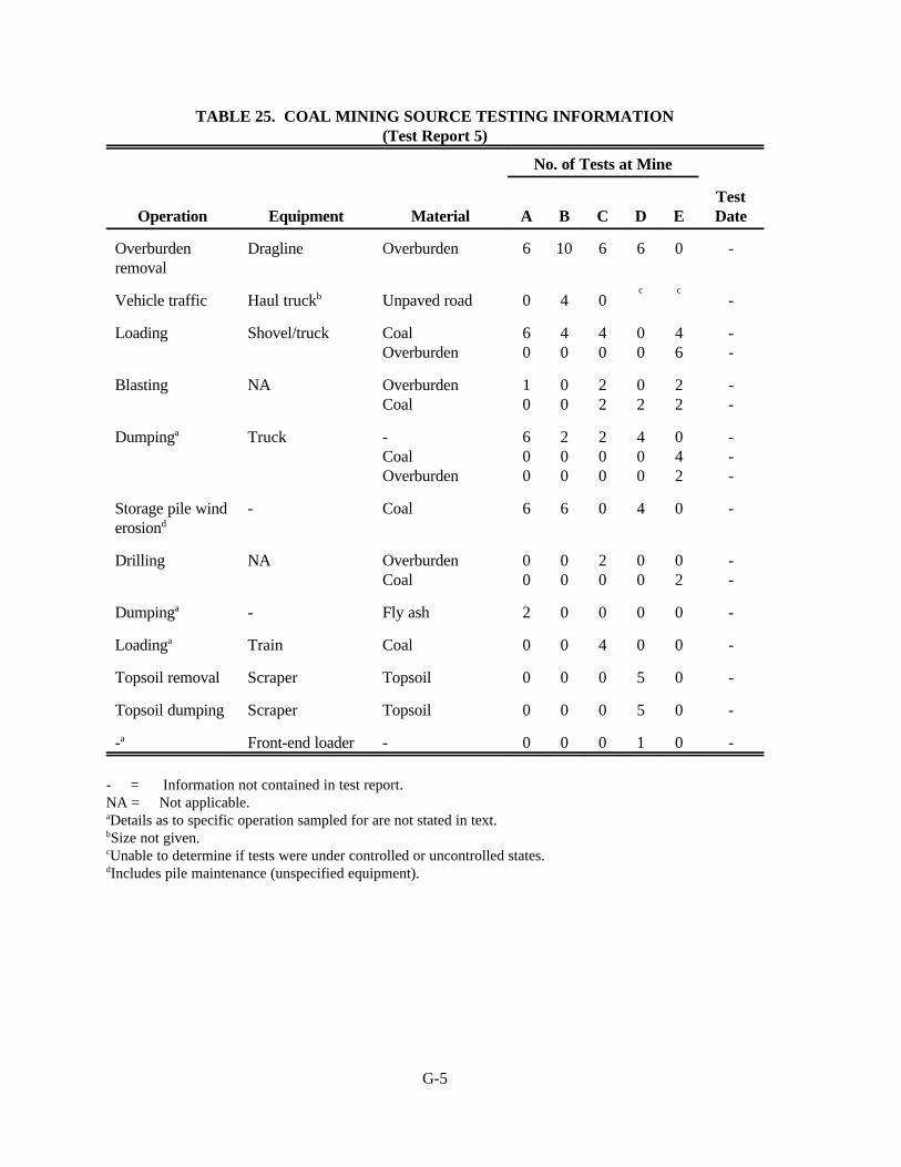
G-5
TABLE 25. COAL MINING SOURCE TESTING INFORMATION(Test Report 5)
No. of Tests at Mine
Operation Equipment Material A B C D ETestDate
Overburdenremoval
Dragline Overburden 6 10 6 6 0 -
Vehicle traffic Haul truckb Unpaved road 0 4 0c c
-
Loading Shovel/truck CoalOverburden
60
40
40
00
46
--
Blasting NA OverburdenCoal
10
00
22
02
22
--
Dumpinga Truck -CoalOverburden
600
200
200
400
042
---
Storage pile winderosiond
- Coal 6 6 0 4 0 -
Drilling NA OverburdenCoal
00
00
20
00
02
--
Dumpinga - Fly ash 2 0 0 0 0 -
Loadinga Train Coal 0 0 4 0 0 -
Topsoil removal Scraper Topsoil 0 0 0 5 0 -
Topsoil dumping Scraper Topsoil 0 0 0 5 0 -
-a Front-end loader - 0 0 0 1 0 -
- = Information not contained in test report.NA = Not applicable.aDetails as to specific operation sampled for are not stated in text.bSize not given.cUnable to determine if tests were under controlled or uncontrolled states.dIncludes pile maintenance (unspecified equipment).
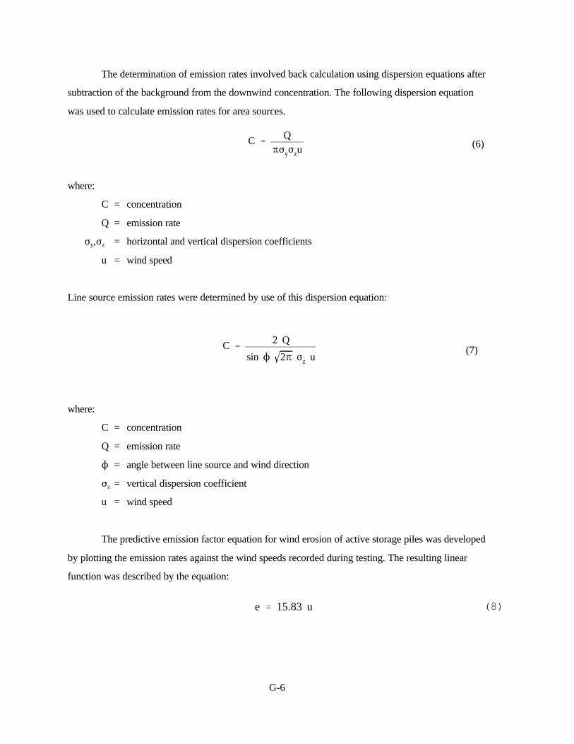
G-6
C 'Q
BFyFzu(6)
C '2 Q
sin N 2B Fz u(7)
e ' 15.83 u (8)
The determination of emission rates involved back calculation using dispersion equations after
subtraction of the background from the downwind concentration. The following dispersion equation
was used to calculate emission rates for area sources.
where:
C = concentration
Q = emission rate
Fy,Fz = horizontal and vertical dispersion coefficients
u = wind speed
Line source emission rates were determined by use of this dispersion equation:
where:
C = concentration
Q = emission rate
N = angle between line source and wind direction
Fz = vertical dispersion coefficient
u = wind speed
The predictive emission factor equation for wind erosion of active storage piles was developed
by plotting the emission rates against the wind speeds recorded during testing. The resulting linear
function was described by the equation:

G-7
lb(acre)(hr)
where:
e = emission rate (lb/hr)
u = wind speed (m/sec)
This equation was then converted to one with units of by assuming storage pile surface
areas of 10 acres.
This upwind-downwind sampling system does not meet the minimum requirements for point
sources as set forth in Section 4.3 since particulate concentrations at only one crosswind distance were
observed. Also details on the operations tested are frequently sketchy. Therefore, with three exceptions
the test data are rated B. The test data for haul roads are rated A, because sampling at multiple
crosswind distances is not required when testing line sources. The test data for storage pile wind
erosion (and maintenance) are rated C because of: (a) the very light winds encountered; (b) the large
size of the piles; and (c) the lack of information on pile maintenance activities. The test data for
blasting are rated C because of the difficulty of quantifying the plume with ground based samplers.
The report indicates that emission factor variation between mines for the same operation is
relatively high; therefore, it was recommended (in the report) that the factors be mine (type) specific.
The following list describes the location of the five mines. The report gives a more in-depth
description of each mine including production rate, stratigraphic data, coal analysis data, surface
deposition, storage capacity, and blasting data.
Mine Area
A Northwest Colorado
B Southwest Wyoming
C Southeast Montana
D Central North Dakota
E Northeast Wyoming
Tables 26 through 30 present the average emission factors determined at each mine along with
the ranges of conditions tested and the associated emission factor ratings. The text indicates that the
emission factors should be used with a fallout function for distances closer than 5 km; however, the
text does not explicitly state what particulate size range is represented by the emission factors.

G-8
1.6 u lb(acre)(hr)
TABLE 26. COAL MINING EMISSION FACTORS (MINE TYPE A), RANGE OF TESTCONDITIONS, AND RATINGS
(Test Report 5)
Range of Conditions
OperationNumberof Tests
Wind Speed(mph)
Moisture(%)
TSP EmissionFactora,b
RatingCode Rating
Dragline 6 0.4-1.8 - 0.0056 lb/yd3 4 D
Shovel/truck loading(coal)
6 0.4-1.3 10 0.014 lb/T 4 D
Blasting (overburden) 1 2.4 - 1,690c lb/blast 9 E
Truck dumpd
(bottom)6 0.4-2.7 - 0.014 lb/T 4 D
Storage pile erosione 6 0.5-2.6 10 1f Cf
Fly ash dump 2 1.5 - 3.9 lb/hr 7/8 E
- = Information not contained in test report.aParticle size not explicitly stated in test report.bEmission factors are from page 2, Table 1 of test report.cText indicates this value represents a maximum rate.dMaterial not given.eu = Wind speed in m/sec. This factor includes emissions from pile maintenance.fRating code refers to Table 5. Rating based on combined data Mines A, B, and D.

G-9
1.6 u lb(acre)(hr)
TABLE 27. COAL MINING EMISSION FACTORS (MINE TYPE B), RANGE OF TESTCONDITIONS, AND RATINGS
(Test Report 5)
Range of Conditions
OperationNumberof Tests
Wind Speed(mph)
Moisture(%)
TSP EmissionFactora,b
RatingCode Rating
Dragline 10 3.1-5.8 - 0.053 lb/yd3 4 D
Haul road 4 3.7-4.7 - 17.0 lb/VMT 5 C
Shovel/truck loading(coal)
4 0.4-0.6 18 0.007 lb/T 5 D
Truck dump(bottom)
2 3.7 - 0.020 lb/T 7 E
Storage pile erosionc 6 0.8-7.6 18 1d Cd
- = Information not contained in test report.aParticle size not explicitly stated in test report.bEmission factors are from page 2, Table 1 of test report.cu = Wind speed in m/sec. This factor includes emissions from pile maintenance.dRating code refers to Table 5. Rating based on combined data Mines A, B, and D.
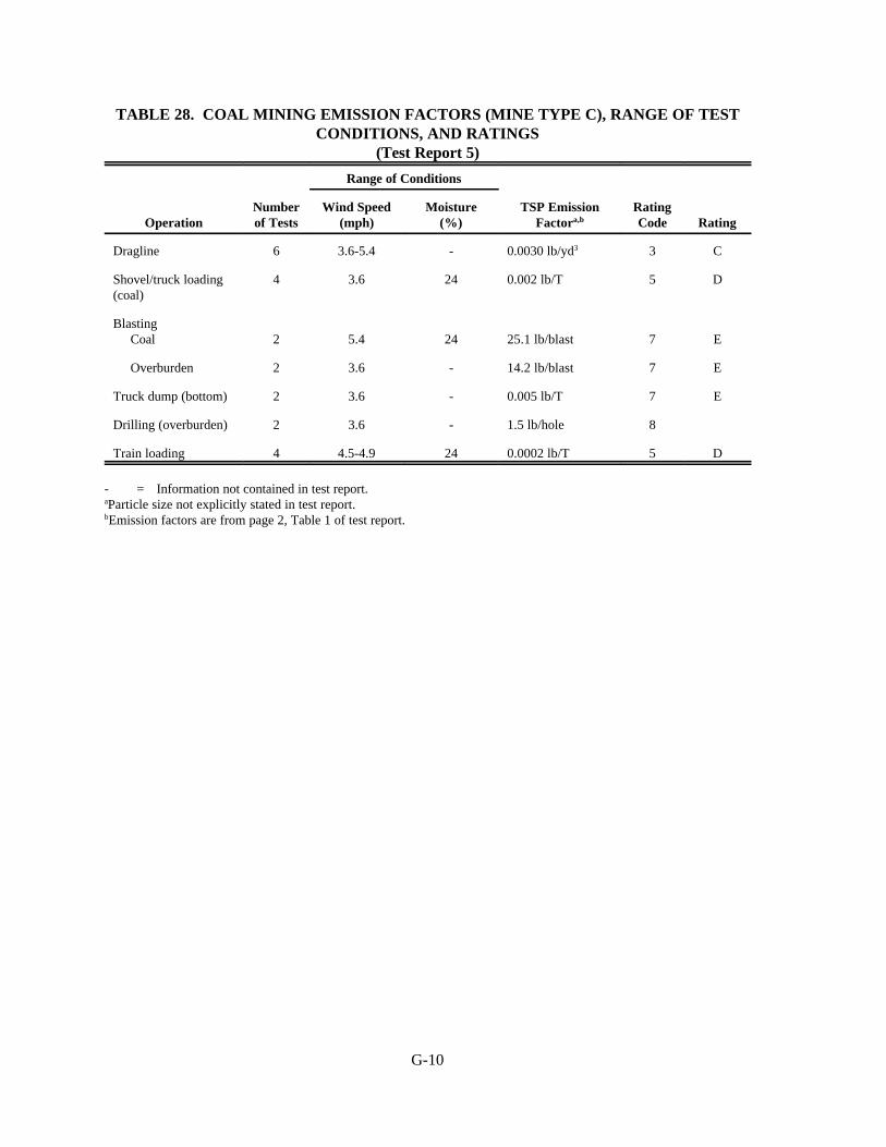
G-10
TABLE 28. COAL MINING EMISSION FACTORS (MINE TYPE C), RANGE OF TESTCONDITIONS, AND RATINGS
(Test Report 5)
Range of Conditions
OperationNumberof Tests
Wind Speed(mph)
Moisture(%)
TSP EmissionFactora,b
RatingCode Rating
Dragline 6 3.6-5.4 - 0.0030 lb/yd3 3 C
Shovel/truck loading(coal)
4 3.6 24 0.002 lb/T 5 D
BlastingCoal 2 5.4 24 25.1 lb/blast 7 E
Overburden 2 3.6 - 14.2 lb/blast 7 E
Truck dump (bottom) 2 3.6 - 0.005 lb/T 7 E
Drilling (overburden) 2 3.6 - 1.5 lb/hole 8
Train loading 4 4.5-4.9 24 0.0002 lb/T 5 D
- = Information not contained in test report.aParticle size not explicitly stated in test report.bEmission factors are from page 2, Table 1 of test report.
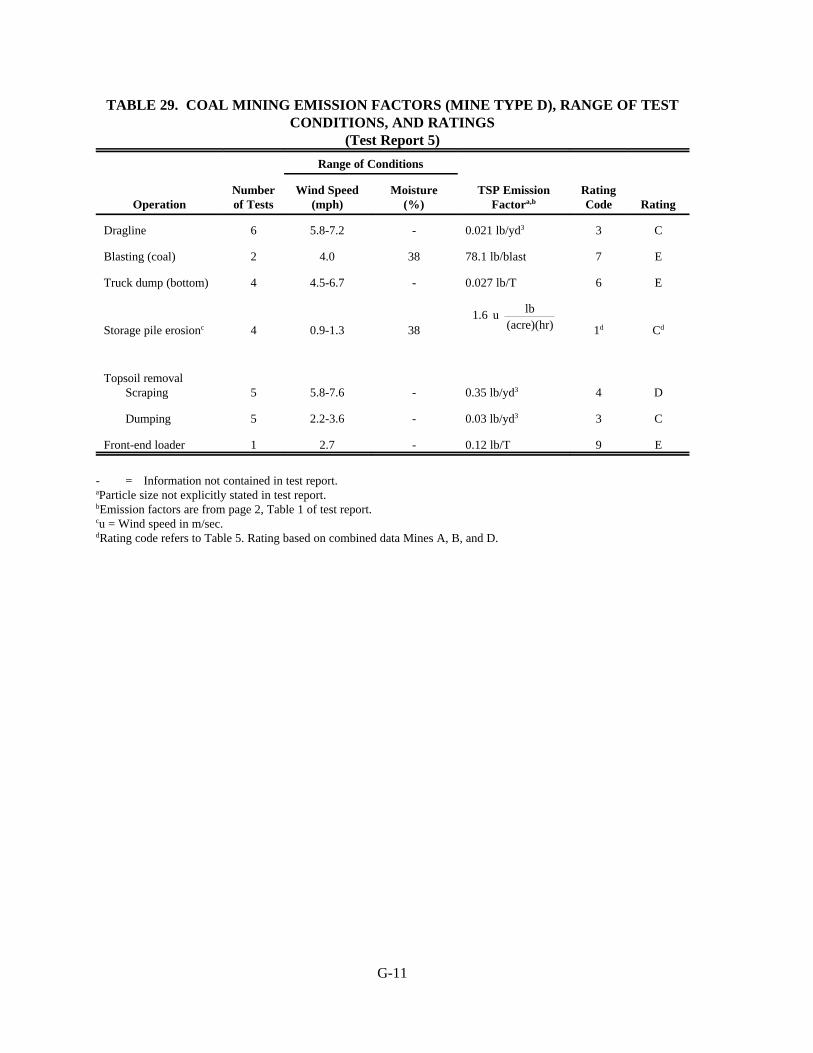
G-11
1.6 u lb(acre)(hr)
TABLE 29. COAL MINING EMISSION FACTORS (MINE TYPE D), RANGE OF TESTCONDITIONS, AND RATINGS
(Test Report 5)
Range of Conditions
OperationNumberof Tests
Wind Speed(mph)
Moisture(%)
TSP EmissionFactora,b
RatingCode Rating
Dragline 6 5.8-7.2 - 0.021 lb/yd3 3 C
Blasting (coal) 2 4.0 38 78.1 lb/blast 7 E
Truck dump (bottom) 4 4.5-6.7 - 0.027 lb/T 6 E
Storage pile erosionc 4 0.9-1.3 38 1d Cd
Topsoil removalScraping 5 5.8-7.6 - 0.35 lb/yd3 4 D
Dumping 5 2.2-3.6 - 0.03 lb/yd3 3 C
Front-end loader 1 2.7 - 0.12 lb/T 9 E
- = Information not contained in test report.aParticle size not explicitly stated in test report.bEmission factors are from page 2, Table 1 of test report.cu = Wind speed in m/sec.dRating code refers to Table 5. Rating based on combined data Mines A, B, and D.

G-12
TABLE 30. COAL MINING EMISSION FACTORS (MINE TYPE E), RANGE OF TESTCONDITIONS, AND RATINGS
(Test Report 5)
Range of Conditions
OperationNumberof Tests
Wind Speed(mph)
Moisture(%)
TSP EmissionFactora,b
RatingCode Rating
Shovel/truck loadingCoal 4 2.3-2.5 30 0.0035 lb/T 5 D
Overburden 6 2.7-3.6 30 0.037 lb/T 3 C
BlastingCoal
2 2.6 30 72.4 lb/blast 7 E
Overburden 2 3.7 - 85.3 lb/blast 7 E
Truck dumpOverburden
2 6.2 - 0.002 lb/T 8 E
Coal (end dump) 4 2.7-3.1 30 0.007 lb/T 6 E
Drilling (coal) 2 4.1 30 0.22 lb/hole 8 E
- = Information not contained in test report.aParticle size not explicitly stated in test report.bEmission factors are from page 2, Table 1 of test report.

G-13
The rating codes in Tables 26 through 30 refer to Table 5 (wind erosion) and Table 4 (all other
sources). Because the single-valued factors were intended to apply only to the specific mine types,- the
requirement for more than one test site was waived. The rating for the equation developed for storage
pile wind erosion (and maintenance) is applicable when the equation is applied to mine types A, B. or
D.
5.5.3 Test Report 14 (1981)
This study was conducted to determine improved fugitive dust emission factors for Western
surface coal mines. Field testing was conducted in three coal fields; Powder River Basin (Mine 1),
North Dakota (Mine 2), and Four Corners (Mine 3). The testing was performed during 1979 and
1980. Table 31 lists the testing information for this study.
The primary sampling method was exposure profiling. When source configuration made it
necessary, alternate methods were used, including upwind-downwind, balloon, and quasi-stack
sampling. Particle size distributions were determined by use of dichotomous samplers. Other
equipment utilized were: (a) high volume samplers for determining upwind concentrations; (b) dustfall
buckets for determining downwind particulate deposition; and (c) recording wind instruments to
determine mean wind speed and direction for adjusting the exposure profiler to isokinetic sampling
conditions and for use in upwind-downwind calculations.
Exposure profiling was used to measure emissions from moving point sources (see Table 31).
The exposure profiling sampling system was similar to that described in Section 5.1.1 and therefore
meets the minimum system design requirements. The upwind-downwind sampling system consisted
generally of 15 particulate collection devices; 5 dichotomous samplers and 10 Hi-vols.
One Hi-vol and one dichotomous sampler were placed upwind while the remaining
instruments were placed at multiple downwind and crosswind distances. This system also meets the
minimum upwind-downwind requirements as described in Section 4.3.

G-14
TABLE 31. COAL MINING SOURCE TESTING INFORMATION (Test Report 14)
Operation Equipment MaterialTest
Methoda Site (mine) Test Dates No. of Tests
Drilling NA Overburden Quasi-stack 1, 3 7/79, 8/79,12/79, 7/80
30
Blasting NA Coal Balloonb 1, 2, 3 8/79,10/79,7/80, 8/80
14
Overburden Balloonb 1, 3 8/79, 8/80 4
Loading Shovel/truck Coal Uw-Dw 1, 2 8/79, 10/79 10
Front-endloader/truck
Coal Uw-Dw 3 7/80, 8/80 15
Dozing Dozer Coal Uw-Dw 1, 2, 3 8/79, 10/79,8/80
12
Overburden Uw-Dw 1, 2, 3 8/79, 10/79,7/80, 8/80
15
Dragline Dragline Overburden Uw-Dw 1, 2, 3 8/79, 10/79,7/80, 8/80
19
Vehicletraffic
Haul truck Unpaved road Uw-Dw 1 8/79, 12/79 11
Unpaved road Profiling 1, 2 ,3 7/79, 8/79,12/79
21
Light-medium duty
Unpaved road Profiling 1, 2, 3 8/79, 10/79,8/80
10
Scrapersc (travel mode)
Scraper Unpavedsurface
Uw-Dw 1 7/79 5
Unpavedsurface
Profiling 1, 2, 3 7/79, 10/79,12/79, 8/80
15
Grading GraderUnpavedsurface
Profiling 2, 3 10/79, 8/80 7
- = Information not contained in test report.NA = Not applicable.aUw-Dw = Upwind-downwind.bThis is actually a modified version of exposure profiling.cLoading and dumping not tested.
G-15
The test data were collected using a well documented sound methodology and, therefore, are
rated A for line sources and for drilling. The test data for coal loading, dozing, and dragline operations
are rated B because of the poorly defined plume characteristics and the interference of the pit areas
with plume dispersion. For blasting the test data are rated C because of the difficulty of quantifying
the large plume with a single line of samplers.
Table 32 presents the average emission factors, range of test conditions, and ratings assigned
for Test Report 14. These single-valued factors were determined by substituting geometric means of
the test conditions into a set of predictive emission factor equations also developed in the study. The
equations are listed in Table 33. The rating codes in Table 32 refer to Table 4, and the codes in
Table 33 refer to Table 5.
5.5.4 Test Report 15 (1981)
A portion of this study was devoted to the development of surface coal mining emission
factors. Field testing was performed from August 1978 through the summer of 1979 at two surface
coal mines located in the Powder River Basin of Wyoming. Table 34 presents the source testing
information for this study.
The test methods employed to develop emission factors were: upwind-downwind, profiling,
and a tracer technique. Particle sizing was performed by optical microscopy of exposed Millipore
filters.
The profiling technique employed in this study was actually a variation of the exposure
profiling procedure described in Section 5.1.1 (Test Report 7). High volume samplers were used
instead of directional isokinetic intakes; therefore, the emission rates determined by profiling were for
TSP (total suspended particulate).
The tracer technique utilized arrays of Bach high-volume samplers and tracer samplers with a
straightforward calculation scheme. These sampling systems meet the minimum requirements as set
forth in Section 4.3; therefore; the test data are rated A.
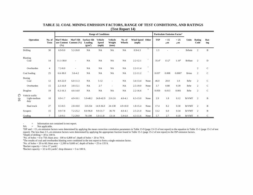
G-16
TABLE 32. COAL MINING EMISSION FACTORS, RANGE OF TEST CONDITIONS, AND RATINGS(Test Report 14)
Range of Conditions Particulate Emission Factora
Operation No. ofTests
Mat’l Moist-ure Content
(%)
Mat’l SiltContent (%)
Surface SiltLoading(g/m2)
VehicleSpeed(mph)
VehicleWeight(tons)
No. ofWheels
Wind Speed(mph)
Other TSP < 15FFm
< 25FFm
Units RatingCode
Rat-ing
Drilling 30 6.9-9.0 5.2-26.8 NA NA NA NA 0.9-6.3b
1.3 - - lb/hole 2 B
BlastingCoal 14 11.1-38.0 - NA NA NA NA 2.2-12.1
c35.4d 13.2d 1.10d lb/blast 2 D
Overburden 4 7.2-8.0 - NA NA NA NA 2.2-11.4e
2 C
Coal loading 25 6.6-38.0 3.6-4.2 NA NA NA NA 2.2-11.2f
0.037 0.008 0.0007 lb/ton 2 C
DozingCoal 12 4.0-22.0 6.0-11.3 NA 5-12 - NA 3.4-13.4 None 46.0 20.0 1.0 lb/hr 2 C
Overburden 15 2.2-16.8 3.8-15.1 NA 2-7 - NA 2.5-19.0 None 3.7 0.88 0.39 lb/hr 2 C
Dragline 19 0.2-16.3 4.6-14.0 NA NA NA NA 2.2-16.6g
0.059 0.013 0.001 lb/hr 2 C
Vehicle trafficLight-mediumduty
10 0.9-1.7 4.9-10.1 5.9-48.2 24.8-42.9 2.0-2.6 4.0-4.1 6.5-13.0 None 2.9 1.8 0.12 lb/VMT 2 B
Haul truck 27 0.3-8.5 2.8-18.0 3.8-254 14.9-36.0 24-138 4.9-10.0 1.8-15.4 None 17.4 8.2 0.30 lb/VMT 2 B
Scrapers 15 0.9-7.8 7.2-25.2 8.0-96.8 9.9-31.7 36-70 4.0-4.1 2.5-21.0 None 13.2 6.0 0.34 lb/VMT 2 B
Grading 7 1.0-9.1 7.2-29.0 76-190 5.0-11.8 13-14 5.9-6.0 4.3-11.6 None 5.7 2.7 0.18 lb/VMT 4 C
- = Information not contained in test report.NA = Not applicable.aISP and < 15 Fm emission factors were determined by applying the mean correction correlation parameters in Table 13-9 (page 13-15 of test report) to the equation in Table 15-1 (page 15-2 of testreport). The less than 2.5 Fm emission factors were determined by applying the appropriate fraction found in Table 15-1 (page 15-2 of test report) to the ISP emission factors.bDepth of drilling = 30 to 100 ft.cNo. of holes = 6 to 750; blast area - 100 to 6,800 m2; depth of holes = 20 to 70 ft.dThe results of coal and overburden blasting were combined in the test report to form a single emission factor.eNo. of holes = 20 to 60; blast area = 2,200 to 9,600 m2; depth of holes = 25 to 135 ft.fBucket capacity = 14 to 17 yards3.gBucket capacity = 32 to 65 yards3; drop distance = 5 to 100 ft.

G-17
961 (A)0.8
(D)1.8 (M)1.9
0.119
(M)0.9
78.4 (s)1.2
(M)1.3
5.7 (s)1.2
(M)1.3
1.0 (s)1.5
(M)1.4
0.0021 (d)1.1
(M)0.3
0.0021 (d)0.7
(M)0.3
2.7 x 10&5 (s)1.3 (W)2.4 6.2 x 10&6 (s)1.4 (W)2.5
0.040 (S)2.5 0.051 (S)2.0
5.79
(M)4.0
3.22
(M)4.3
0.0067 (w)3.4 (L)0.2 0.0051 (w)3.5
TABLE 33. COAL MINING EMISSION FACTOR EQUATIONS AND RATINGS(Test Report 14)
Particulate Emission Factor Equationa
Operation TSP < 15 FFm < 2.5 FFm/TSPb Units RatingCode
Rating
Blasting (coalor overburden)
2,550 (A)0.6
(D)1.5 (M)2.30.030 lb/blast 1 C
Coal loading1.16
(M)1.2 0.019 lb/ton 1 B
DozingCoal
18.6 (s)1.5
(M)1.4 0.022 lb/hr 1 B
Overburden 0.105 lb/hr 1 B
DraglineOverburden 0.017 lb/yard3 1 B
Scrapers(Travelmode)
0.026 lb/VMT 1 A
Grading 0.031 lb/VMT 2 B
Vehicle trafficLight-mediumduty
0.040 lb/VMT 2 B
Haul trucks 0.017 lb/VMT 1 A
Note: The range of test conditions are as stated in Table 32. Particle diameters are aerodynamic.aFrom page 15-2, Table 15-1 of test report.bMultiply this fraction by the TSP predictive equation to determine emissions in the < 2.5 Fm size range.
A = area blasted (ft2) d = drop height (ft)
M = moisture content (%) W = vehicle weight (tons)
D = hole depth (ft) S = vehicle speed (mph)
s = silt content (%) w = number of wheels
L = silt loading (g/m2)

G-18
TABLE 34. COAL MINING SOURCE TESTING INFORMATION (Test Report 15)
Operation Equipment Material Test MethodaSite No.(mine) Test Dates
No.of
Tests
Vehicle traffic Haul trucks Coal overburden Profiling 2 Winter, spring,summer
26b
Dumping - Coal Tracer 1, 2 Fall, winter 3
Loading Train Coal Tracer 1, 2 Fall 2
Overburdenreplacement
- Overburden Uw-Dw 1, 2 Winter, spring,summer
7
Topsoil removal (Scraper)c Topsoil Uw-Dw 1 Summer 2
Exposed Area NA Seeded land,strippedoverburden, gradedoverburden
Uw-Dw 1, 2 Spring, summer 18
- = Information not contained in test report.NA = Not applicable.aUw-Dw = Upwind-downwind.bThis series of tests involved a wide variety of road conditions ranging from total control (wet) to totally uncontrolled(dry). An emission factor equation was derived which takes the amount of control present into account (see Table 33,footnote a).cAlthough scrapers are most often used in this operation the test report did not explicitly state that scrapers were beingused.
G-19
Vd ' 1.51 (x)&0.588 (9)
The upwind-downwind sampling system consisted of 10 Hi-Vols of which two were placed
upwind and eight were placed at multiple downwind and crosswind distances. Wind direction and
speed were concurrently measured at an on-site station for all test periods. This sampling system
meets the minimum requirements set forth in Section 4.3. However, the emission factors are rated B
because these operations tested (overburden replacement, coal dumping, and top soil removal) were
not described as to the equipment employed (see Table 34).
The calculated TSP emission rates were modified with a depletion factor, as follows. A
deposition velocity was determined from dustfall bucket measurements:
where:
Vd = deposition velocity
x = distance downwind of source
This velocity was combined with stability class and wind speed to derive a depletion factor in terms of
distance downwind of a particulate source. The actual emission rate for an operation was then
calculated through division of the apparent emission rate (measured at a particular distance
downwind) by the appropriate depletion factor.
Table 35 gives the range of test conditions, emission factors, and applicable ratings for Test
Report 16. The rating codes refer to Table 4. These ratings overlook the particle size incompatibility
between the Hi-Vol measurements of particulate flux and the dustfall measurements of deposition
velocity.

G-20
TABLE 35. COAL MINING EMISSION FACTORS, RANGE OF TEST CONDITIONS,AND RATINGS(Test Report 15)
OperationNumberof Tests
Mat’lMois-ture
Content(%)
Mat’lSilt
Con-tent(%)
Veh-icle
Speed(mph)
VehicleWeight(tons)
WindSpeed(mph)
TotalParticu-
lateEmission
Factor Units
Rat-ingCod
eRat-ing
Vehicle traffica 26 Dry-wet 8.3-11.2
22-24 - 3.6-19.2 22.0 lb/VMT 4 C
Coal dumpingb 3 - - NA NA 2.9-6.0 0.066 lb/T 6 D
Train loadingc 2 - - NA NA 4.0-11.4 0.027 lb/T 7 D
Overburdenreplacementd
7 - - - - 3.8-19.9 0.012 lb/T 3 C
Topsoil removala 2 - - - - 10.1 0.058 lb/T 8 E
Exposed areasf 18 - - NA NA 5.4-17.4 0.38 ton/acre-year
2 C
- =Information not contained in test report.
NA =Not applicable.
aThe emission factor equation derived for this source is from page 35 of test report. It was evaluated at zero wettings per hour.bEmission factor is from page 46, Table 5.1 of test report.cEmission factor is from page 47, Table 5.2 of test report.dEmission factor is from page 52, Table 6.1 of test report.eEmission factor is from page 52, Table 6.2 of test report.fEmission factor is from page 55, Table 7.1 of test report.
G-21
8.5 Western Surface Coal Mining and Processing
Since no emission factors are currently presented in AP-42 for coal mining. The predictive
emission factor equations presented in Table 49 are recommended for inclusion in AP-42 under a
section named “Western Surface Coal Mining.” Table SO presents the single-valued emission factors
for western surface coal mining. It is recommended that for any source operation not covered by the
equations in Table 49, the highest rated single valued factors from Table 50 be incorporated in AP-42.
All of the recommended factors may be applied to Eastern surface coal mining. However,
each should then be aerated one letter value (e.g., C to D).
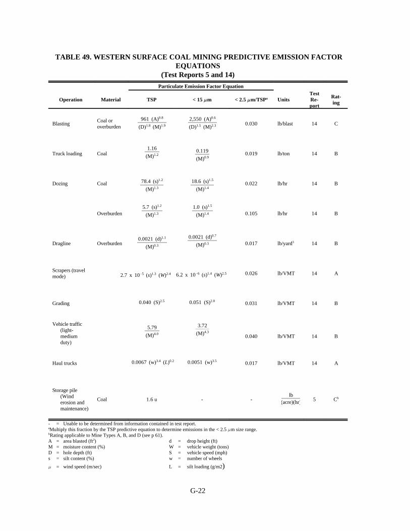
G-22
961 (A)0.8
(D)1.8 (M)1.9
0.0021 (d)1.1
(M)0.3
2,550 (A)0.6
(D)1.5 (M)2.3
1.16
(M)1.20.119
(M)0.9
78.4 (s)1.2
(M)1.3
18.6 (s)1.5
(M)1.4
5.7 (s)1.2
(M)1.3
1.0 (s)1.5
(M)1.4
0.0021 (d)0.7
(M)0.3
2.7 x 10&5 (s)1.3 (W)2.4 6.2 x 10&6 (s)1.4 (W)2.5
0.040 (S)2.5 0.051 (S)2.0
3.72
(M)4.3
0.0067 (w)3.4 (L)0.2 0.0051 (w)3.5
lb(acre)(hr)
5.79
(M)4.0
TABLE 49. WESTERN SURFACE COAL MINING PREDICTIVE EMISSION FACTOREQUATIONS
(Test Reports 5 and 14)
Particulate Emission Factor Equation
Operation Material TSP < 15 FFm < 2.5 FFm/TSPa UnitsTestRe-port
Rat-ing
BlastingCoal oroverburden
0.030 lb/blast 14 C
Truck loading Coal 0.019 lb/ton 14 B
Dozing Coal 0.022 lb/hr 14 B
Overburden 0.105 lb/hr 14 B
Dragline Overburden 0.017 lb/yard3 14 B
Scrapers (travelmode)
0.026 lb/VMT 14 A
Grading 0.031 lb/VMT 14 B
Vehicle traffic(light-mediumduty)
0.040 lb/VMT 14 B
Haul trucks 0.017 lb/VMT 14 A
Storage pile(Winderosion andmaintenance)
Coal 1.6 u - - 5 Cb
- = Unable to be determined from information contained in test report.aMultiply this fraction by the TSP predictive equation to determine emissions in the < 2.5 Fm size range.bRating applicable to Mine Types A, B, and D (see p 61).A = area blasted (ft2) d = drop height (ft)M = moisture content (%) W = vehicle weight (tons)D = hole depth (ft) S = vehicle speed (mph)s = silt content (%) w = number of wheels
F = wind speed (m/sec) L = silt loading (g/m2)

G-23
TABLE 50. WESTERN SURFACE COAL MINING SINGLE-VALUED EMISSION FACTORS(Test Report 4, 5, 14, and 15)
Emission Factor by Aerodynamic Diameter
Operation Source (Material) Total TSP< 30(FFm)
< 15(FFm)
< 10(FFm)
< 5(FFm)
< 2.5(FFm) Units Test Report Rating
Drilling(Overburden)
(mine type C)(Coal)
(mine type E)
-
-
1.3
0.22
-
-
-
-
-
-
-
-
-
-
lb/hole
lb/hole
14
5
B
E
Blasting (Overburden)(mine type A)(mine type C)(mine type E)
(Coal)(mine type C)(mine type D)(mine type E)
---
---
1,69014.285.3
25.178.172.4
---
---
---
---
---
---
---
---
---
---
lb/blastlb/blastlb/blast
lb/blastlb/blastlb/blast
555
555
E*E*E*
E*E*E*
Dragline (Overburden)(mine type A)(mine type B)(mine type C)(mine type D)
----
0.00560.0530.00300.021
----
----
----
----
----
lb/yd3
lb/yd3
lb/yd3
lb/yd3
5555
D*D*C*C*
Top soil removal Scraper(mine type D)
Unspecifiedequipment
--
0.440.058
--
--
--
--
--
lb/Tlb/T
515
DE
Overburdenreplacement
Unspecifiedequipment
- 0.012 - - - - - lb/T 15 C
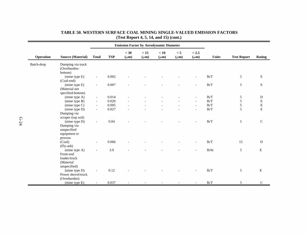
G-24
TABLE 50. WESTERN SURFACE COAL MINING SINGLE-VALUED EMISSION FACTORS(Test Report 4, 5, 14, and 15) (cont.)
Emission Factor by Aerodynamic Diameter
Operation Source (Material) Total TSP< 30(FFm)
< 15(FFm)
< 10(FFm)
< 5(FFm)
< 2.5(FFm) Units Test Report Rating
Batch-drop Dumping via truck(Overburden-bottom)
(mine type E)(Coal-end)
(mine type E)(Material notspecified-bottom)
(mine type A)(mine type B)(mine type C)(mine type D)
Dumping viascraper (top soil)
(mine type D)Dumping viaunspecifiedequipment orprocess(Coal)(Fly-ash)
(mine type A)Front-endloader/truck(Materialunspecified)
(mine type D)Power shovel/truck(Overburden)
(mine type E)
-
-
----
-
-
-
-
-
0.002
0.007
0.0140.0200.0050.027
0.04
0.066
3.9
0.12
0.037
-
-
----
-
-
-
-
-
-
-
----
-
-
-
-
-
-
-
----
-
-
-
-
-
-
-
----
-
-
-
-
-
-
-
----
-
-
-
-
-
lb/T
lb/T
lb/Tlb/Tlb/Tlb/T
lb/T
lb/T
lb/hr
lb/T
lb/T
5
5
5555
5
15
5
5
5
E
E
DEEE
C
D
E*
E*
C
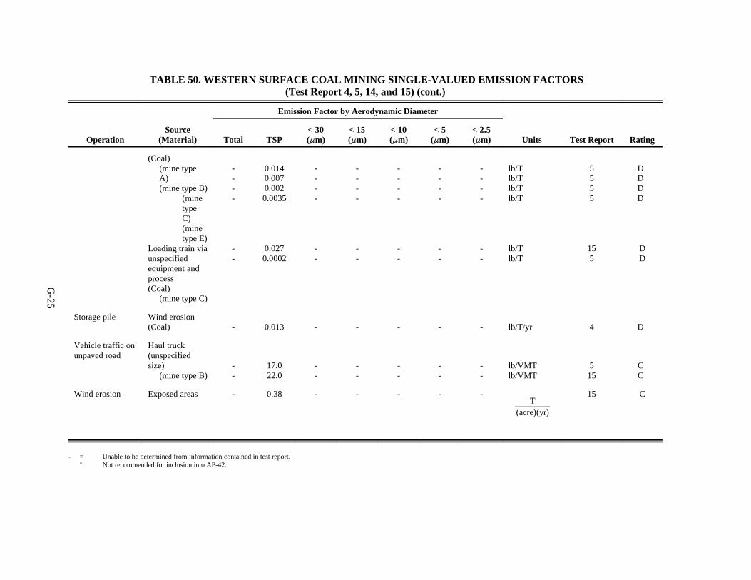
G-25
T(acre)(yr)
TABLE 50. WESTERN SURFACE COAL MINING SINGLE-VALUED EMISSION FACTORS(Test Report 4, 5, 14, and 15) (cont.)
Emission Factor by Aerodynamic Diameter
OperationSource
(Material) Total TSP< 30(FFm)
< 15(FFm)
< 10(FFm)
< 5(FFm)
< 2.5(FFm) Units Test Report Rating
(Coal)(mine typeA)(mine type B)
(minetypeC)(minetype E)
Loading train viaunspecifiedequipment andprocess(Coal)
(mine type C)
----
--
0.0140.0070.0020.0035
0.0270.0002
----
--
----
--
----
--
----
--
----
--
lb/Tlb/Tlb/Tlb/T
lb/Tlb/T
5555
155
D*D*D*D*
DD
Storage pile Wind erosion(Coal) - 0.013 - - - - - lb/T/yr 4 D*
Vehicle traffic onunpaved road
Haul truck(unspecifiedsize)
(mine type B)--
17.022.0
--
--
--
--
--
lb/VMTlb/VMT
515
C*C*
Wind erosion Exposed areas - 0.38 - - - - - 15 C
- = Unable to be determined from information contained in test report.* = Not recommended for inclusion into AP-42.

G-26
G.2 Section 7 of EPA report "Improved Emission Factors for Fugitive Dust From Western
Surface Coal Mining Sources--Volume I - Sampling Methodology and Test Results"
SECTION 7
RESULTS FOR SOURCES TESTED BY EXPOSURE PROFILING
SUMMARY OF TESTS PERFORMED
As previously discussed, exposure profiling was used to test particulate emissions from haul
trucks, light-duty and medium-duty vehicles, scrapers (travel mode) and graders. These sources were
tested at three mines during the period July 1979 through August 1980.
A total of 63 successful exposure profiling tests were conducted at the three mines/four visits.
They were distributed by source and by mine as follows:
Number of Tests
Source
Controlled/
Uncontrolled Mine 1 Mine 2 Mine 1W Mine 3
Haul trucks U 6 6 3 4
C 0 4 0 5
Light- and med.- duty
vehicles
U 3 4 0 3
C 2 0 0 0
Scrapers U 5 6 2 2
Graders U 0 5 0 2
Light and variable wind conditions were encountered at Mine 1 during the test period July-
August 1979, with winds occasionally reversing and traffic-generated emissions impacting on the
upwind sampling station. These events were termed “bad passes.”
G-27
Table 7-1 lists the site conditions for the exposure profiling tests of dust emissions generated
by haul trucks. The comparability tests are indicated by an asterisk after the run number. In addition
to the testing of uncontrolled sources, watering of haul roads was tested as a control measure.
Table 7-2 gives the road and traffic characteristics for the exposure profiling tests of haul
trucks. This source category exhibited a wide range of road and traffic characteristics, indicating a
good potential for identifying and quantifying correction parameters. Most tests involved a blend of
vehicle types dominated by haul trucks. Silt and moisture values were determined by laboratory
analysis of road surface aggregate samples obtained from the test roads. Mean vehicle speeds and
weights are arithmetic averages for the mixes of vehicles which passed over the test roads during
exposure profiling.
Table 7-3 lists the site conditions for the exposure profiling tests of dust emissions generated
by light- and medium-duty vehicles. In addition to the testing of uncontrolled roads, the application of
calcium chloride to an access road was tested as a control measure.
Table 7-4 gives the road and traffic conditions for the exposure profiling tests of light- and
medium-duty vehicles. Small variations in mean vehicle weight and mean number of vehicle wheels
were observed for this source category. No access roads were available at Mine 2, so light-duty
vehicles were tested at a haul road site.
Table 7-5 lists the site conditions for the exposure profiling tests of dust emissions generated
by scrapers (travel mode). Table 7-6 gives the road and traffic conditions for the exposure profiling
tests of scrapers. All scrapers tested were four-wheeled vehicles, which excluded this parameter from
consideration as a correction factor.
Table 7-7 lists the site conditions for the exposure profiling tests of dust emissions generated
by graders. Table 7-8 gives the road and traffic conditions for the exposure profiling tests of graders.
All graders tested were six-wheeled vehicles and weighed 14 tons. Therefore, mean vehicle weight and
mean number of vehicle wheels were excluded from consideration as correction factors.

G-28
TABLE 7-1. EXPOSURE PROFILING SITE CONDITIONS - HAUL TRUCKS
Profiler Meteorology
Vehicle Passes
Mine/Sitea Runb DateStartTime
SamplingDuration
(min) Good BadTemp(°C)
WindSpeedc
(m/s)
Mine 1/Site 2 J-6 7/30/79 16:06 67 2 37 24.5 0.9
J-9* 8/01/79 10:21 51 41 0 28.3 4.8
J-10* 8/01/79 14:08 52 43 2 31.0 4.4
J-11d 8/01/79 17:39 48 40 0 30.5 4.2
J-12* 8/02/79 10:50 49 18 1 26.7 0.8
J-20* 8/09/79 14:10 49 23 0 23.0 2.5
J-21* 8/09/79 16:51 26 13 1 25.0 1.6
Mine 2/Site 1 K-1 10/11/79 10:21 86 65 0 14.6 6.2
Mine 2/Site 3 (Watered) K-6 10/15/79 11:03 177 84 0 17.8 3.4
Mine 2/Site 3 K-7 10/15/79 14:50 53 57 0 23.5 2.6
Mine 2/Site 3 (Watered) K-8 10/16/79 11:02 105 43 0 10.3 5.7
Mine 2/Site 3 K-9 10/16/79 13:18 89 63 0 12.0 5.0
K-10 10/17/79 10:37 65 40 0 10.6 5.0
K-11 10/17/79 12:05 64 50 0 12.5 5.2
K-12 10/17/79 13:38 58 43 0 15.5 5.4
Mine 2/Site 3 (Watered) K-13 10/23/79 10:47 73 78 0 4.0 3.7
Mine 1/Site 5 L-1 12/07/79 14:04 92 57 0 0.7 1.9
Mine 1/Site 6 L-2 12/08/79 13:12 4e 23f 0 12.2 6.9
L-3 12/08/79 13:45 48 26 0 13.2 6.5
L-4 12/08/79 15:04 47 32 0 13.6 6.1
Mine 3/Site 1 P-1 7/25/80 16:28 57 15 0 35 3.8
Mine 3/Site 2 P-2 7/26/80 10:25 95 10 2 27 1.8
P-3 7/27/80 9:10 89 18 0 27 3.8
Mine 3/Site 2(Watered)
P-4 7/28/80 8:41 135 48 0 27 3.7
Mine 3/Site 2 P-5 7/29/80 7:32 108 38 0 32 2.8

TABLE 7-1. (CONTINUED)
G-29
Mine 3/Site 2(Watered)
P-6 7/30/80 7:12 112 48 0 29 2.2
P-7 7/31/80 7:27 95 35 0 29 2.5
P-8 7/31/80 9:22 103 49 0 29 3.0
P-9 8/01/80 7:51 142 48 0 27 3.7a Mine 1/Site 2 - Mine B tipple road (haul road to crusher).
Mine 2/Site 1 - 250m west of haul truck unloading station.Mine 2/Site 3 - 1 mile west of haul truck unloading station.Mine 1/Site 5 - About 100m east of haul road sites for summer testing.Mine 1/Site 6 - About 250m northeast of haul road sites for summer testing.Mine 2/Site 1 - Near Ramp 5 east of lake.Mine 2/Site 2 - Between Ramps 2 and 3.
bAsterisk indicates comparability test.cValue at 3m above the ground, interpolated from 1.5 and 4.5m warm wire anemometer data using a logarithmic profile.dMRI comparative equipment run; PEDCO did not test.eRepresents total time that the profiler ran properly; there was a prior period for which isokinetic flows could not be obtained.fRepresents the total number of passes during the attempted run (while the equipment, other than the profiler, was operating).
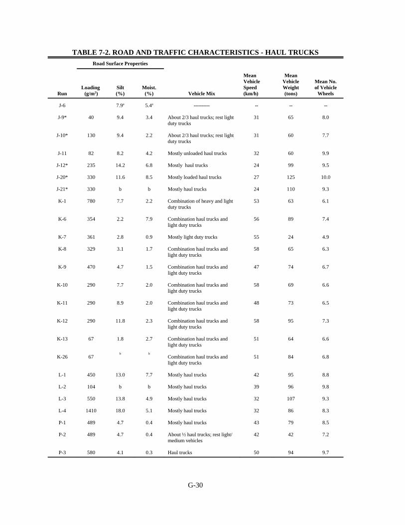
G-30
TABLE 7-2. ROAD AND TRAFFIC CHARACTERISTICS - HAUL TRUCKS
Road Surface Properties
RunLoading
(g/m2)Silt(%)
Moist.(%) Vehicle Mix
MeanVehicleSpeed(km/h)
MeanVehicleWeight(tons)
Mean No.of Vehicle
Wheels
J-6 7.9a 5.4a ---------- -- -- --
J-9* 40 9.4 3.4 About 2/3 haul trucks; rest lightduty trucks
31 65 8.0
J-10* 130 9.4 2.2 About 2/3 haul trucks; rest lightduty trucks
31 60 7.7
J-11 82 8.2 4.2 Mostly unloaded haul trucks 32 60 9.9
J-12* 235 14.2 6.8 Mostly haul trucks 24 99 9.5
J-20* 330 11.6 8.5 Mostly loaded haul trucks 27 125 10.0
J-21* 330 b b Mostly haul trucks 24 110 9.3
K-1 780 7.7 2.2 Combination of heavy and lightduty trucks
53 63 6.1
K-6 354 2.2 7.9 Combination haul trucks andlight duty trucks
56 89 7.4
K-7 361 2.8 0.9 Mostly light duty trucks 55 24 4.9
K-8 329 3.1 1.7 Combination haul trucks andlight duty trucks
58 65 6.3
K-9 470 4.7 1.5 Combination haul trucks andlight duty trucks
47 74 6.7
K-10 290 7.7 2.0 Combination haul trucks andlight duty trucks
58 69 6.6
K-11 290 8.9 2.0 Combination haul trucks andlight duty trucks
48 73 6.5
K-12 290 11.8 2.3 Combination haul trucks andlight duty trucks
58 95 7.3
K-13 67 1.8 2.7 Combination haul trucks andlight duty trucks
51 64 6.6
K-26 67b b
Combination haul trucks andlight duty trucks
51 84 6.8
L-1 450 13.0 7.7 Mostly haul trucks 42 95 8.8
L-2 104 b b Mostly haul trucks 39 96 9.8
L-3 550 13.8 4.9 Mostly haul trucks 32 107 9.3
L-4 1410 18.0 5.1 Mostly haul trucks 32 86 8.3
P-1 489 4.7 0.4 Mostly haul trucks 43 79 8.5
P-2 489 4.7 0.4 About ½ haul trucks; rest light/medium vehicles
42 42 7.2
P-3 580 4.1 0.3 Haul trucks 50 94 9.7
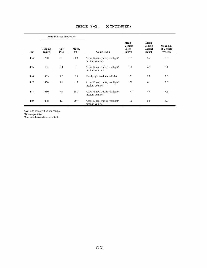
TABLE 7-2. (CONTINUED)
Road Surface Properties
RunLoading
(g/m2)Silt(%)
Moist.(%) Vehicle Mix
MeanVehicleSpeed(km/h)
MeanVehicleWeight(tons)
Mean No.of Vehicle
Wheels
G-31
P-4 200 2.0 0.3 About ½ haul trucks; rest light/medium vehicles
51 55 7.6
P-5 131 3.1 c About ½ haul trucks; rest light/medium vehicles
50 47 7.1
P-6 489 2.8 2.9 Mostly light/medium vehicles 51 25 5.6
P-7 458 2.4 1.5 About ½ haul trucks; rest light/medium vehicles
50 61 7.6
P-8 680 7.7 15.3 About ½ haul trucks; rest light/medium vehicles
47 47 7.5
P-9 438 1.6 20.1 About ½ haul trucks; rest light/medium vehicles
50 58 8.7
aAverage of more than one sample.bNo sample taken.cMoisture below detectable limits.
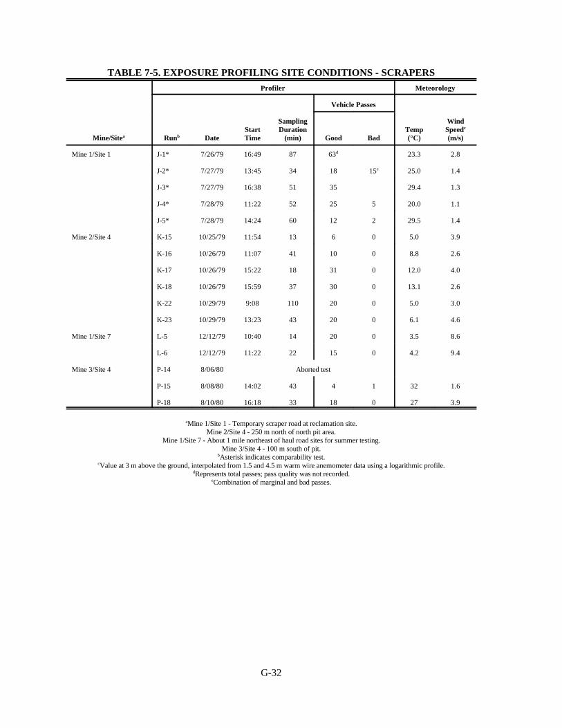
G-32
TABLE 7-5. EXPOSURE PROFILING SITE CONDITIONS - SCRAPERS
Profiler Meteorology
Vehicle Passes
Mine/Sitea Runb DateStartTime
SamplingDuration
(min) Good BadTemp(°C)
WindSpeedc
(m/s)
Mine 1/Site 1 J-1* 7/26/79 16:49 87 63d 23.3 2.8
J-2* 7/27/79 13:45 34 18 15e 25.0 1.4
J-3* 7/27/79 16:38 51 35 29.4 1.3
J-4* 7/28/79 11:22 52 25 5 20.0 1.1
J-5* 7/28/79 14:24 60 12 2 29.5 1.4
Mine 2/Site 4 K-15 10/25/79 11:54 13 6 0 5.0 3.9
K-16 10/26/79 11:07 41 10 0 8.8 2.6
K-17 10/26/79 15:22 18 31 0 12.0 4.0
K-18 10/26/79 15:59 37 30 0 13.1 2.6
K-22 10/29/79 9:08 110 20 0 5.0 3.0
K-23 10/29/79 13:23 43 20 0 6.1 4.6
Mine 1/Site 7 L-5 12/12/79 10:40 14 20 0 3.5 8.6
L-6 12/12/79 11:22 22 15 0 4.2 9.4
Mine 3/Site 4 P-14 8/06/80 Aborted test
P-15 8/08/80 14:02 43 4 1 32 1.6
P-18 8/10/80 16:18 33 18 0 27 3.9
aMine 1/Site 1 - Temporary scraper road at reclamation site.Mine 2/Site 4 - 250 m north of north pit area.
Mine 1/Site 7 - About 1 mile northeast of haul road sites for summer testing.Mine 3/Site 4 - 100 m south of pit.
bAsterisk indicates comparability test.cValue at 3 m above the ground, interpolated from 1.5 and 4.5 m warm wire anemometer data using a logarithmic profile.
dRepresents total passes; pass quality was not recorded.eCombination of marginal and bad passes.

G-33
TABLE 7-6. ROAD AND TRAFFIC CHARACTERISTICS - SCRAPERS
Road Surface Properties
RunLoading
(g/m2)Silt(%)
Moist.(%) Vehicle Mix
MeanVehicleSpeed(km/h)
MeanVehicleWeight(tons)
Mean No.of Vehicle
Wheels
J-1* 121 8.9a 5.7a Mostly scrapers 31 50 4.1
J-2* 313 23.4a 2.3a Mostly scrapers 31 53 4.0
J-3* 310 15.8 4.1 Mostly scrapers 39 54 4.1
J-4* 55 14.6a 1.5a Unloaded scrapers 32 36 4.0
J-5* 310 10.6a 0.9a Loaded scrapers 29 70 4.0
K-15b b b
Mostly unloaded scrapersc 45 46 4.0
K-16 384 25.2d 6.0 All scrapers 48 64 4.0
K-17 384 25.2d 6.0 Mostly scrapers 37 57 4.1
K-18 384 25.2d 6.0 All scrapers 40 66 4.0
K-22 301 21.6 5.4 All unloaded scrapers 51 45 4.0
K-23 318 24.6 7.8 All scrapers 45 54 4.0
L-5 238 21.0e
All scrapers 34 53 4.0
L-6 238 21.0e
All scrapers 32 50 4.0
P-15f
7.2 1.0 Mostly scrapers 26 42 4.0
P-18f
7.2 1.0 Scrapers 16 64 4.0
aAverage of more than one sample.bNo sample taken.cTest stopped prematurely; scraper drivers quit for lunch.dAverage silt of Runs K-19 to K-23.eUnrepresentative sample taken after grader pass; sample not analyzed.fSample not analyzed for loading.

G-34
TABLE 7-7. EXPOSURE PROFILING SITE CONDITIONS - GRADERS
Profiler Meteorology
Vehicle Passes
Mine/Sitea Runb DateStartTime
SamplingDuration
(min) Good BadTemp(°C)
WindSpeedc
(m/s)
Mine 2/Site 4 K-19 10/27/79 10:24 57 40 0 10.2 5.2
K-20 10/27/79 11:46 59 40 0 13.4 4.5
K-21 10/27/79 13:34 49 40 0 17.4 4.3
Mine 2/Site 5 K-24 10/30/79 10:16 35 30 0 6.5 4.4
K-25 10/30/79 11:16 39 30 0 7.8 4.6
Mine 3/Site 4 8/10/80 17:45 129 9 0 27 3.5
P-17 8/10/80 13:28 67 15 0 27 1.9
aMine 2/Site 4 - 250 m north of north pit area.Mine 2/Site 5 - 250 m northwest of haul truck unloading station.
Mine 3/Site 4 - 100 m south of pit.bValue at 3 m above the ground, interpolated from 1.5 and 4.5 m warm wire anemometer data using a logarithmic profile.

G-35
TABLE 7-8. ROAD AND TRAFFIC CHARACTERISTICS - GRADERS
Road Surface Properties
RunLoading
(g/m2)Silt(%)
Moist.(%) Vehicle Mix
MeanVehicleSpeed(km/h)
MeanVehicleWeight(tons)
Mean No.of Vehicle
Wheels
K-19 328 23.1 9.1 All graders 8 14 6.0
K-20 535 29.0 8.8 All graders 10 14 6.0
K-21 495 27.8 7.2 All graders 10 14 6.0
K-24 597 17.6 4.0 Mostly graders 10 13 5.9
K-25 776 24.5 5.4 All graders 10 14 6.0
P-16a
7.2 1.0 Graders 19 14 6.0
P-17a
7.2 1.0 Graders 16 14 6.0
aSample not analyzed for loading.

G-36
RESULTS
The measured emission rates are shown in Tables 7-9 through 7-12 for haul trucks, light- and
medium-duty vehicles, scrapers, and graders, respectively. In each case, emission rates are given for
TP, SP, IP, and FP.
For certain runs, emission rates could not be calculated. For haul truck run L-2, the profiler
samples did not maintain a consistent flow rate. Haul truck run J-6 was not analyzed because of the
predominance of bad passes. The emissions from run J-7, the access road treated with calcium
chloride, were too low to be measured. Scraper run P-15 produced only a TP emission factor;
questionable results from a single dichotomous sampler prevented calculation of reliable emission
rates for SP, IP, and FP.
The means, standard deviations, and ranges of SP emission rates for each source category are
shown below:
SP Emission Rate (lbs/VMT)
Source No. Tests Mean Std. Dev. Range
Haul trucksUncontrolledControlled
199
18.84.88
20.23.44
0.71-67.20.60-8.4
Light- and medium-dutyvehicles
UncontrolledControlled
102
4.160.35a
3.73a
0.64-9.0a
ScrapersUncontrolled 14 57.8 95.3 3.9-355
GradersUncontrolled 7 9.03 11.2 1.8-34.0
a On one of two tests, the emissions were below detectable limits.
As expected, the SP emission rates for controlled road sources were substantially lower than for
uncontrolled sources. The mean emission rate for watered haul roads was 26 percent of the mean for
uncontrolled haul roads. For light- and medium-duty vehicles, the mean emission rate for roads treated
with calcium chloride was 8 percent of the mean for uncontrolled roads.
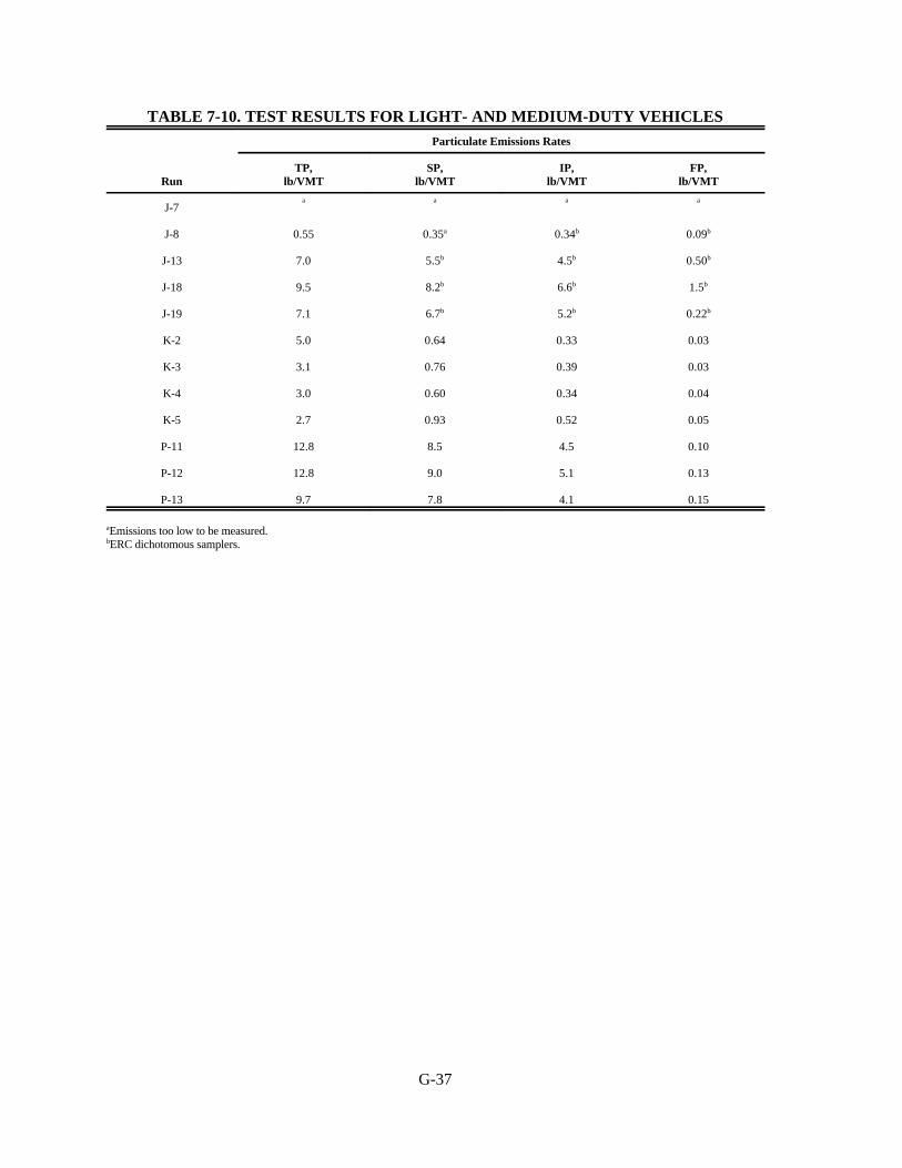
G-37
TABLE 7-10. TEST RESULTS FOR LIGHT- AND MEDIUM-DUTY VEHICLES
Particulate Emissions Rates
RunTP,
lb/VMTSP,
lb/VMTIP,
lb/VMTFP,
lb/VMT
J-7a a a a
J-8 0.55 0.35a 0.34b 0.09b
J-13 7.0 5.5b 4.5b 0.50b
J-18 9.5 8.2b 6.6b 1.5b
J-19 7.1 6.7b 5.2b 0.22b
K-2 5.0 0.64 0.33 0.03
K-3 3.1 0.76 0.39 0.03
K-4 3.0 0.60 0.34 0.04
K-5 2.7 0.93 0.52 0.05
P-11 12.8 8.5 4.5 0.10
P-12 12.8 9.0 5.1 0.13
P-13 9.7 7.8 4.1 0.15
aEmissions too low to be measured.bERC dichotomous samplers.

G-38
TABLE 7-11. TEST RESULTS FOR SCRAPERSParticulate Emission Rates
RunaTP,
lb/VMTSP,
lb/VMTIP,
lb/VMTFP,
lb/VMT
J-1* 41.4 8.6 4.2 0.27
J-2* 66.5 9.4 4.0 0.19
J-3* 125 50.2 26.1 1.5
J-4* 27.5 3.9 1.7 0.09
J-5* 96.7 17.7 10.0 1.4
K-15 126 16.2 7.2 0.39
K-16 206 29.2 15.6 1.8
K-17 232 74.3 35.6 1.6
K-18 179 43.0 19.3 0.81
K-22 58.4 10.3 4.8 0.29
K-23 118 24.5 11.1 0.54
L-5 360b 355b 217b 0.72b
L-6 184 163 94.0 1.0
P-15 383c c c
P-18 18.8d 4.0d 1.4d 0.02d
aAsterisk indicates comparability test.bProfiler samplers malfunctioned.cOnly one dichotomous sampler and only four good passes.dOnly two profilers operational.
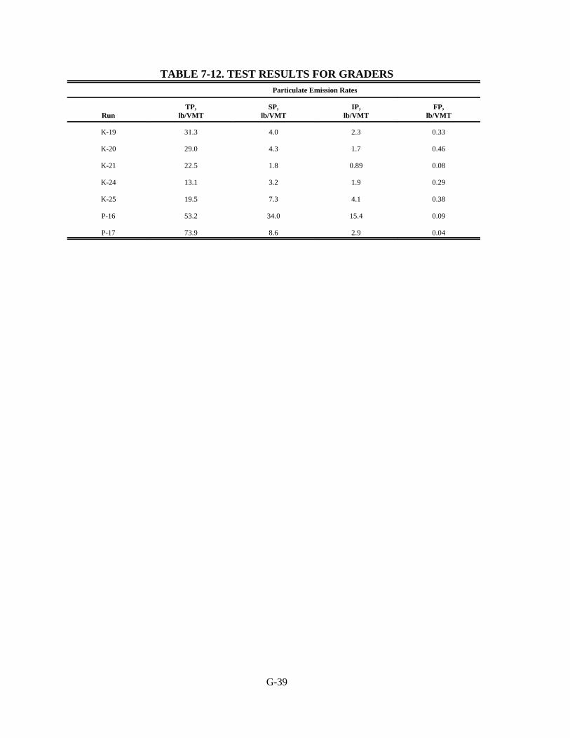
G-39
TABLE 7-12. TEST RESULTS FOR GRADERSParticulate Emission Rates
RunTP,
lb/VMTSP,
lb/VMTIP,
lb/VMTFP,
lb/VMT
K-19 31.3 4.0 2.3 0.33
K-20 29.0 4.3 1.7 0.46
K-21 22.5 1.8 0.89 0.08
K-24 13.1 3.2 1.9 0.29
K-25 19.5 7.3 4.1 0.38
P-16 53.2 34.0 15.4 0.09
P-17 73.9 8.6 2.9 0.04

G-40
The average ratios of IF and FP to SP emission rates are:
SourceAverage Ratio of IP to
SP Emission RatesAverage Ratio of FP to
SP Emission Rates
Haul trucks 0.50 0.033
Light- and medium-duty vehicles 0.63 0.112
Scrapers 0.49 0.026
Graders 0.48 0.055
As indicated, SP emissions from light- and medium-duty vehicles contained a much larger proportion
of small particles than did the other source categories.
The measured dustfall rates are shown in Tables 7-13 through 7-16 for haul trucks, light- and
medium-duty vehicles, scrapers, and graders, respectively.
Flux data from collocated samplers are given for the upwind sampling location and for three
downwind distances. The downwind dustfall fluxes decay sharply with distance from the source.
PROBLEMS ENCOUNTERED
Adverse meteorology created the most frequent difficulties in sampling emissions from
unpaved roads. Isokinetic sampling cannot be achieved with the existing profilers when wind speeds are
less than 4 mph. Problems of light winds occurred mostly during the summer testing at Mine 1. In
addition, wind direction shifts resulted in source plume impacts on the upwind samplers on several
occasions. These events, termed "bad passes," were confined for the most part to summer testing at
Mine 1.
Bad passes were not counted in determining source impact on downwind samplers. Measured
upwind particulate concentrations were adjusted to mean observed upwind concentrations for adjoining
sampling periods at the same site when no bad passes occurred.
Another problem encountered was mining equipment breakdown or reassignment. On several
occasions sampling equipment had been deployed but testing could not be conducted because the
mining vehicle activity scheduled for the test road did not occur.
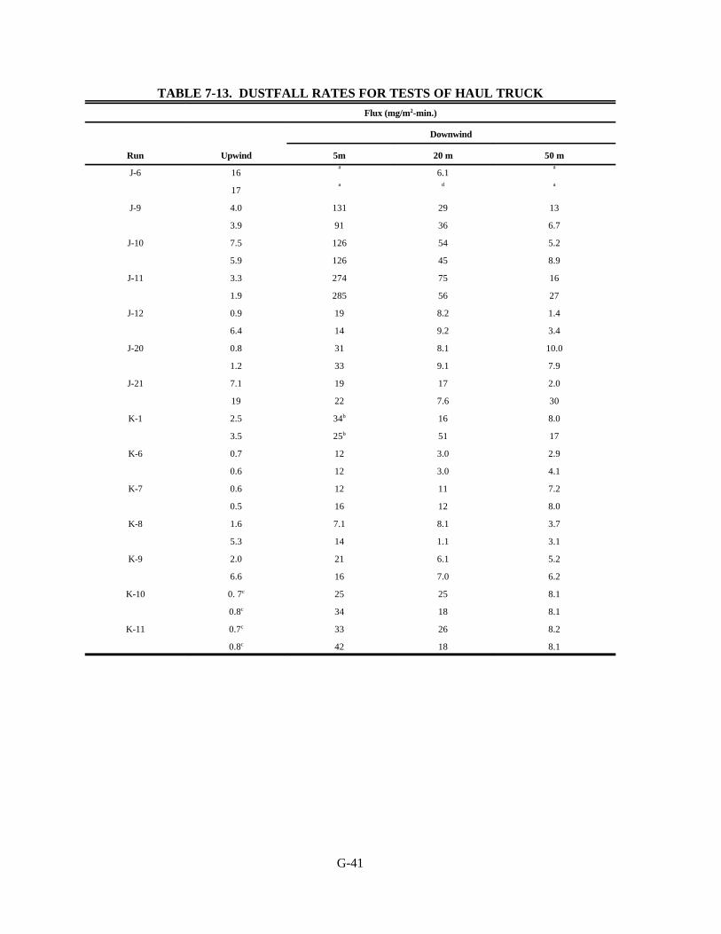
G-41
TABLE 7-13. DUSTFALL RATES FOR TESTS OF HAUL TRUCK
Flux (mg/m2-min.)
Downwind
Run Upwind 5m 20 m 50 m
J-6 16a
6.1a
17a d a
J-9 4.0 131 29 13
3.9 91 36 6.7
J-10 7.5 126 54 5.2
5.9 126 45 8.9
J-11 3.3 274 75 16
1.9 285 56 27
J-12 0.9 19 8.2 1.4
6.4 14 9.2 3.4
J-20 0.8 31 8.1 10.0
1.2 33 9.1 7.9
J-21 7.1 19 17 2.0
19 22 7.6 30
K-1 2.5 34b 16 8.0
3.5 25b 51 17
K-6 0.7 12 3.0 2.9
0.6 12 3.0 4.1
K-7 0.6 12 11 7.2
0.5 16 12 8.0
K-8 1.6 7.1 8.1 3.7
5.3 14 1.1 3.1
K-9 2.0 21 6.1 5.2
6.6 16 7.0 6.2
K-10 0. 7c 25 25 8.1
0.8c 34 18 8.1
K-11 0.7c 33 26 8.2
0.8c 42 18 8.1
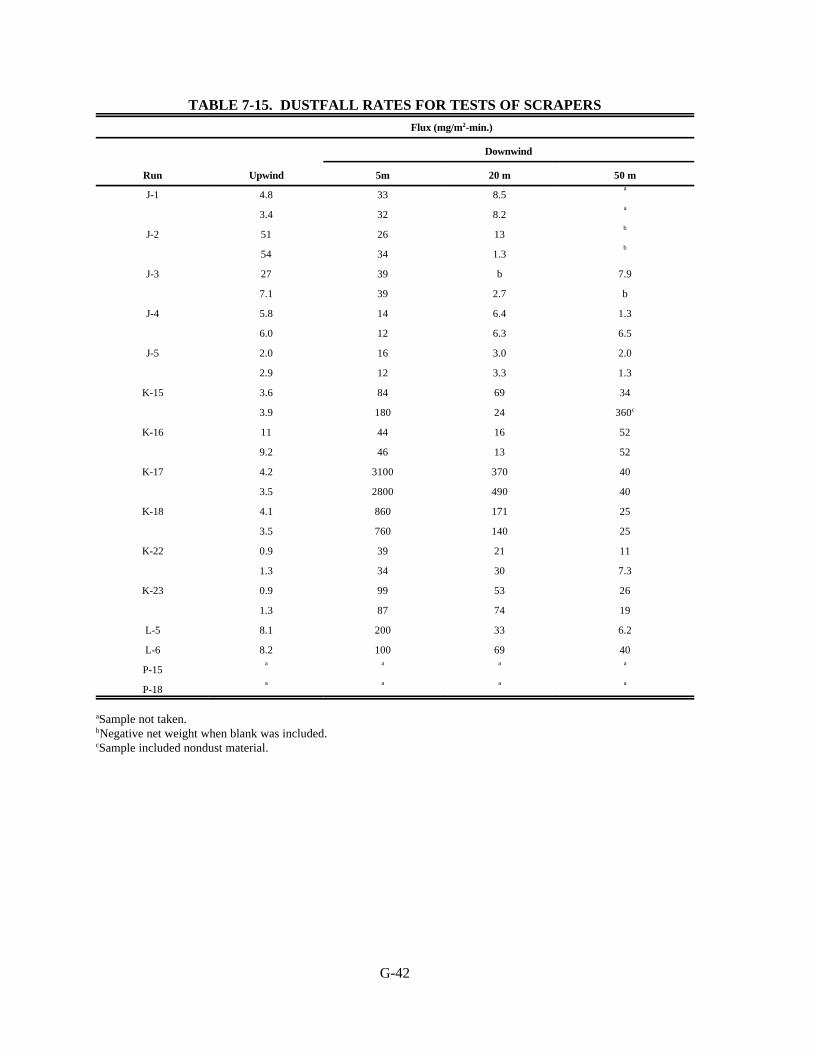
G-42
TABLE 7-15. DUSTFALL RATES FOR TESTS OF SCRAPERS
Flux (mg/m2-min.)
Downwind
Run Upwind 5m 20 m 50 m
J-1 4.8 33 8.5a
3.4 32 8.2a
J-2 51 26 13b
54 34 1.3b
J-3 27 39 b 7.9
7.1 39 2.7 b
J-4 5.8 14 6.4 1.3
6.0 12 6.3 6.5
J-5 2.0 16 3.0 2.0
2.9 12 3.3 1.3
K-15 3.6 84 69 34
3.9 180 24 360c
K-16 11 44 16 52
9.2 46 13 52
K-17 4.2 3100 370 40
3.5 2800 490 40
K-18 4.1 860 171 25
3.5 760 140 25
K-22 0.9 39 21 11
1.3 34 30 7.3
K-23 0.9 99 53 26
1.3 87 74 19
L-5 8.1 200 33 6.2
L-6 8.2 100 69 40
P-15a a a a
P-18a a a a
aSample not taken.bNegative net weight when blank was included.cSample included nondust material.

G-43
TABLE 7-16. DUSTFALL RATES FOR TESTS OF GRADERS
Flux (mg/m2-min.)
Downwind
Run Upwind 5m 20 m 50 m
K-19 2.5 46 52 28
2.6 75 36 18
K-20 2.6 20 53 28
2.7 25 37 19
K-21 2.6 65 62 34
2.7 56 43 22
K-24 2.7 64 49 23
4.5 48 40 16
K-25 2.8 61 46 22
4.7 46 39 15
P-16a
22 2.9 0.2a
22 9.8 6.6
P-17a
21 6.1 6.6a
27 10 9.9
aSample not taken
H-1
Appendix HMaterials Related to Active Storage Pile Emission Factor
This appendix contains information related to emission factors for active storage piles. The
information is from Sections 5.5 and 8.5 of EPA report “Fugitive Dust Emission Factor Update for AP42"
and Section 10 of EPA report “Improved Emission Factors For Fugitive Dust From Western Surface Coal
Mining Sources - Volume I - Sampling Methodology and Test Results.”

H-2
TABLE OF CONTENTS
Page
H.1 Sections 5.5 and 8.5 of EPA report "Fugitive Dust Emission Factor Update for AP-42" . . . . . . . . . . . . . . . . . . . . . . . . . . . . . . . . . . . . . . . . . . . . . . . . . . . . . . . . . . . H-3
H.2 Section 10 of EPA report "Improved Emission Factors For Fugitive Dust FromWestern Surface Coal Mining Sources --Volume I - Sampling Methodologyand Test Results" . . . . . . . . . . . . . . . . . . . . . . . . . . . . . . . . . . . . . . . . . . . . . . . . . . . . . . H-22

H-3
H.1 Section 5.5 of EPA report "Fugitive Dust Emission Factor Update for AP-42"
5.5 Section 8.24 - Western Surface Coal Mining and Processing
5.5.1 Test Report 4 (1977)
This study developed an emission factor for coal storage only. Four tests at one coal storage pile(location not given) were conducted using the upwind-downwind technique. Table 23 presents the sourcetesting information for this study.
High-volume samplers were used to collect the airborne particulates from one upwind and fourdownwind positions. The wind parameters were recorded at 15-min intervals. A sampling array similar tothat described in Section 5.3.2 (Test Report 6) was employed in this study. This sampling system meetsthe minimum requirements of the upwind-downwind sampling technique. Optical microscopy wasemployed to determine a particle size distribution. However, the particle size distribution for the emissionfactor was determined from particle counting only (not mass fraction), which is unrepresentative of a masssize distribution.
This methodology is of generally sound quality; and emission rates were determined in a similarmanner to that described in Section 5.3.2 (Test Report 6). However, the report lacks sufficient detail foradequate validation. For example, no indication is given as to sampling height. Also the field datarecorded at the sampling stations are not presented. The test data are therefore rated B
Table 24 presents the developed emission factor, conditions tested and the appropriate rating. Onlyone pile was sampled, although it was two different sizes during testing. The rating code refers to Table 4.
5.5.2 Test Report 5 (1978)
This study was directed to the development of emission factors for the surface coal miningindustry. Testing was conducted at five Western coal mines (Mines A through E). Table 25 presents thedistribution of tests performed.
The upwind-downwind method was used with standard high-volume samplers for particulatecollection. Wind parameters were continuously measured at a fixed location within each mine. A hand-held wind speed indicator was used when possible to record data at the exact test site. Optical microscopywas employed to determine particle size distribution.
The upwind-downwind sampler deployment used in this study generally employed six samplers foreach test; additionally, six more samplers were operated at a second height in half the tests to determine avertical plume gradient. Two instruments were located upwind of a source to measure backgroundconcentrations while four instruments were located downwind. These downwind samplers were deployedalong a straight line (the assumed plume centerline) at four different distances.
The determination of emission rates involved back calculation using dispersion equations aftersubtaction of the background from the downwind concentration. The following dispersion equation wasused to calculate emission rates for area sources.
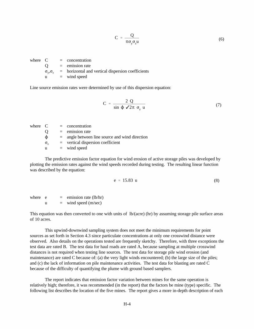
H-4
C 'Q
BFyFzu(6)
C '2 Q
sin N T2B Fz u (7)
e ' 15.83 u (8)
where C = concentrationQ = emission rateFy,Fz = horizontal and vertical dispersion coefficientsu = wind speed
Line source emission rates were determined by use of this dispersion equation:
where C = concentrationQ = emission rateN = angle between line source and wind directionFz = vertical dispersion coefficientu = wind speed
The predictive emission factor equation for wind erosion of active storage piles was developed byplotting the emission rates against the wind speeds recorded during testing. The resulting linear functionwas described by the equation:
where e = emission rate (lb/hr)u = wind speed (m/sec)
This equation was then converted to one with units of lb/(acre) (hr) by assuming storage pile surface areasof 10 acres.
This upwind-downwind sampling system does not meet the minimum requirements for pointsources as set forth in Section 4.3 since particulate concentrations at only one crosswind distance wereobserved. Also details on the operations tested are frequently sketchy. Therefore, with three exceptions thetest data are rated B. The test data for haul roads are rated A, because sampling at multiple crosswinddistances is not required when testing line sources. The test data for storage pile wind erosion (andmaintenance) are rated C because of: (a) the very light winds encountered; (b) the large size of the piles;and (c) the lack of information on pile maintenance activities. The test data for blasting are rated Cbecause of the difficulty of quantifying the plume with ground based samplers.
The report indicates that emission factor variation between mines for the same operation isrelatively high; therefore, it was recommended (in the report) that the factors be mine (type) specific. Thefollowing list describes the location of the five mines. The report gives a more in-depth description of each
H-5
mine including production rate, stratigraphic data, coal analysis data, surface deposition, storage capacity,and blasting data.
Mine Area
A Northwest ColoradoB Southwest WyomingC Southeast MontanaD Central North DakotaE Northeast Wyoming
Tables 26 through 30 present the average emission factors determined at each mine along with theranges of conditions tested and the associated emission factor ratings. The text indicates that the emissionfactors should be used with a fallout function for distances closer than 5 km; however, the text does notexplicitly state what particulate size range is represented by the emission factors.
The rating codes in Tables 26 through 30 refer to Table 5 (wind erosion) and Table 4 (all othersources). Because the single-valued factors were intended to apply only to the specific mine types, therequirement for more than one test site was waived. The rating for the equation developed for storage pilewind erosion (and maintenance) is applicable when the equation is applied to mine types A, B. or D.
5.5.3 Test Report 14 (1981)
This study was conducted to determine improved fugitive dust emission factors for Westernsurface coal mines. Field testing was conducted in three coal fields; Powder River Basin (Mine 1), NorthDakota (Mine 2), and Four Corners (Mine 3). The testing was performed during 1979 and 1980. Table 31lists the testing information for this study.
The primary sampling method was exposure profiling. When source configuration made itnecessary, alternate methods were used, including upwinddownwind, balloon, and quasi-stack sampling. Particle size distributions were determined by use of dichotomous samplers. Other equipment utilizedwere: (a) high volume samplers for determining upwind concentrations; (b) dustfall buckets for determiningdownwind particulate deposition; and (c) recording wind instruments to determine mean wind speed anddirection for adjusting the exposure profiler to isokinetic sampling conditions and for use in upwind-downwind calculations.
Exposure profiling was used to measure emissions from moving point sources (see Table 31). Theexposure profiling sampling system was similar to that described in Section 5.1.1 and therefore meets theminimum system design requirements. The upwind-downwind sampling system consisted generally of15 particulate collection devices; 5 dichotomous samplers and 10 Hi-vols.
One Hi-Vol and one dichotomous sampler were placed upwind while the remaining instrumentswere placed at multiple downwind and crosswind distances. This system also meets the minimum upwind-downwind requirements as described in Section 4.3.
The test data were collected using a well documented sound methodology and, therefore, are ratedA for line sources and for drilling. The test data for coal loading, dozing, and dragline operations are ratedB because of the poorly defined plume characteristics and the interference of the pit areas with plume
H-6
Vd ' 1.51 (x)&0.588 (9)
dispersion. For blasting the test data are rated C because of the difficulty of quantifying the large plumewith a single line of samplers.
Table 32 presents the average emission factors, range of test conditions, and ratings assigned forTest Report 14. These single-valued factors were determined by substituting geometric means of the testconditions into a set of predictive emission factor equations also developed in the study. The equations arelisted in Table 33. The rating codes in Table 32 refer to Table 4, and the codes in Table 33 refer toTable 5.
5.5.4 Test Report 15 (1981)
A portion of this study was devoted to the development of surface coal mining emission factors. Field testing was performed from August 1978 through the summer of 1979 at two surface coal mineslocated in the Powder River Basin of Wyoming. Table 34 presents the source testing information for thisstudy.
The test methods employed to develop emission factors were: upwinddownwind, profiling, and atracer technique. Particle sizing was performed by optical microscopy of exposed Millipore filters.
The profiling technique employed in this study was actually a variation of the exposure profilingprocedure described in Section 5.1.1 (Test Report 7). High volume samplers were used instead ofdirectional isokinetic intakes; therefore, the emission rates determined by profiling were for TSP (totalsuspended particulate).
The tracer technique utilized arrays or both high-volume samplers and t lacer samplers with astraightforward calculation scheme. These sampling systems meet the minimum requirements as set forthin Section 4.3; therefore; the test data are rated A.
The upwind-downwind sampling system consisted of 10 Hi-Vols of which two were placed upwindand eight were placed at multiple downwind and crosswind distances. Wind direction and speed wereconcurrently measured at an on-site station for all test periods. This sampling system meets the minimumrequirements set forth in Section 4.3. However, the emission factors are rated B because these operationstested (overburden replacement, coal dumping, and top soil removal) were not described as to theequipment employed (see Table 34).
The calculated TSP emission rates were modified with a depletion factor, as follows. A depositionvelocity was determined from dustfall bucket measurements:
where Vd = deposition velocityx = distance downwind of source
This velocity was combined with stability class and wind speed to derive a depletion factor in termsof distance downwind of a particulate source. The actual emission rate for an operation was thencalculated through division of the apparent emission rate (measured at a particular distance downwind) bythe appropriate depletion factor.

H-7
Table 35 gives the range of test conditions, emission factors, and applicable ratings for TestReport 16. The rating codes refer to Table 4. These ratings overlook the particle size incompatibilitybetween the Hi-Vol measurements of particulate flux and the dustfall measurements of deposition velocity.
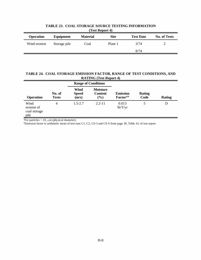
H-8
TABLE 23. COAL STORAGE SOURCE TESTING INFORMATION(Test Report 4)
Operation Equipment Material Site Test Date No. of Tests
Wind erosion Storage pile Coal Plant 1 3/74 2
8/74
TABLE 24. COAL STORAGE EMISSION FACTOR, RANGE OF TEST CONDITIONS, ANDRATING (Test Report 4)
Range of Conditions
OperationNo. ofTests
WindSpeed(m/s)
MoistureContent
(%)EmissionFactora,b
RatingCode Rating
Winderosion ofcoal storagepile
4 1.5-2.7 2.2-11 0.013lb/T/yr
5 D
aFor particles < 10, Fm (physical diameter).bEmission factor is arithmetic mean of test runs C1, C2, CS-3 and CS-S from page 30, Table A1 of test report.
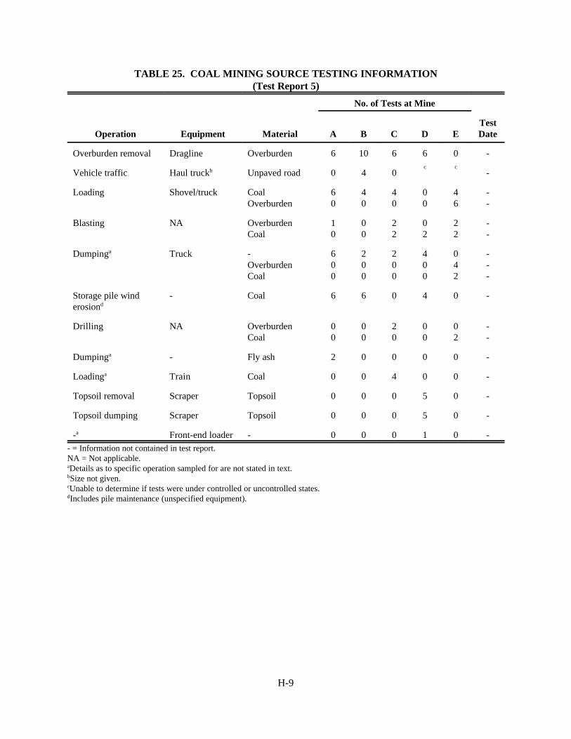
H-9
TABLE 25. COAL MINING SOURCE TESTING INFORMATION(Test Report 5)
No. of Tests at Mine
Operation Equipment Material A B C D ETestDate
Overburden removal Dragline Overburden 6 10 6 6 0 -
Vehicle traffic Haul truckb Unpaved road 0 4 0c c
-
Loading Shovel/truck CoalOverburden
60
40
40
00
46
--
Blasting NA OverburdenCoal
10
00
22
02
22
--
Dumpinga Truck -OverburdenCoal
600
200
200
400
042
---
Storage pile winderosiond
- Coal 6 6 0 4 0 -
Drilling NA OverburdenCoal
00
00
20
00
02
--
Dumpinga - Fly ash 2 0 0 0 0 -
Loadinga Train Coal 0 0 4 0 0 -
Topsoil removal Scraper Topsoil 0 0 0 5 0 -
Topsoil dumping Scraper Topsoil 0 0 0 5 0 -
-a Front-end loader - 0 0 0 1 0 -- = Information not contained in test report.NA = Not applicable.aDetails as to specific operation sampled for are not stated in text.bSize not given.cUnable to determine if tests were under controlled or uncontrolled states.dIncludes pile maintenance (unspecified equipment).

H-10
TABLE 26. COAL MINING EMISSION FACTORS (MINE TYPE A), RANGE OF TESTCONDITIONS, AND RATINGS
(Test Report 5)Range of Conditions
OperationNumberof Tests
Wind Speed(mph) Moisture (%)
TSP EmissionFactora,b
RatingCode Rating
Dragline 6 0.4-1.8 - 0.0056 lb/yd3 4 D
Shovel/truck loading(coal)
6 0.4-1.3 10 0.014 lb/T 4 D
Blasting (overburden) 1 2.4 - 1,690c lb/blast 9 E
Truck dumpd
(bottom)6 0.4-2.7 - 0.014 lb/T 4 D
Storage pile erosione 6 0.5-2.6 10 1.6 u lb(acre)(hr)
1f Cf
Fly ash dump 2 1.5 - 3.9 lb/hr 7/8 E- = Information not contained in test report.aParticle size not explicitly stated in test report.bEmission factors are from page 2, Table 1 of test report.cText indicates this value represents a maximum rate.dMaterial not given.eu = Wind speed in m/sec. This factor includes emissions from pile maintenance.fRating code refers to Table 5. Rating based on combined data Mines A, B, and D.
TABLE 27. COAL MINING EMISSION FACTORS (MINE TYPE B), RANGE OF TESTCONDITIONS, AND RATINGS
(Test Report 5)Range of Conditions
OperationNumberof Tests
Wind Speed(mph) Moisture (%)
TSP EmissionFactora,b
RatingCode Rating
Dragline 10 3.1-5.8 - 0.053 lb/yd3 4 D
Haul road 4 3.7-4.7 - 17.0 lb/VMT 5 C
Shovel/truck loading(coal)
4 0.4-0.6 18 0.007 lb/T 5 D
Truck dump(bottom)
2 3.7 - 0.020 lb/T 7 E
Storage pile erosionc 6 0.8-7.6 18 1.6 u lb(acre)(hr)
1d Cd
- = Information not contained in test report.aParticle size not explicitly stated in test report.bEmission factors are from page 2, Table 1 of test report.cu = Wind speed in m/sec. This factor includes emissions from pile maintenance.dRating code refers to Table 5. Rating based on combined data Mines A, B, and D.

H-11
TABLE 28. COAL MINING EMISSION FACTORS (MINE TYPE C), RANGE OF TESTCONDITIONS, AND RATINGS
(Test Report 5)Range of Conditions
OperationNumberof Tests
Wind Speed(mph) Moisture (%)
TSP EmissionFactora,b
RatingCode Rating
Dragline 6 3.6-5.4 - 0.0030 lb/yd3 3 C
Shovel/truck loading(coal)
4 3.6 24 0.002 lb/T 5 D
BlastingCoal 2 5.4 24 25.1 lb/blast 7 E
Overburden 2 3.6 - 14.2 lb/blast 7 E
Truck dump (bottom) 2 3.6 - 0.005 lb/T 7 E
Drilling (overburden) 2 3.6 - 1.5 lb/hole 8
Train loading 4 4.5-4.9 24 0.0002 lb/T 5 D- = Information not contained in test report.aParticle size not explicitly stated in test report.bEmission factors are from page 2, Table 1 of test report.
TABLE 29. COAL MINING EMISSION FACTORS (MINE TYPE D), RANGE OF TESTCONDITIONS, AND RATINGS
(Test Report 5)Range of Conditions
OperationNumberof Tests
Wind Speed(mph) Moisture (%)
TSP EmissionFactora,b
RatingCode Rating
Dragline 6 5.8-7.2 - 0.021 lb/yd3 3 C
Blasting (coal) 2 4.0 38 78.1 lb/blast 7 E
Truck dump (bottom) 4 4.5-6.7 - 0.027 lb/T 6 E
Storage pile erosionc 4 0.9-1.3 38 1.6 u lb(acre)(hr)
1d Cd
Topsoil removalScraping 5 5.8-7.6 - 0.35 lb/yd3 4 D
Dumping 5 2.2-3.6 - 0.03 lb/yd3 3 C
Front-end loader 1 2.7 - 0.12 lb/T 9 E- = Information not contained in test report.aParticle size not explicitly stated in test report.bEmission factors are from page 2, Table 1 of test report.cu = Wind speed in m/sec.dRating code refers to Table 5. Rating based on combined data Mines A, B, and D.

H-12
TABLE 30. COAL MINING EMISSION FACTORS (MINE TYPE E), RANGE OF TESTCONDITIONS, AND RATINGS
(Test Report 5)Range of Conditions
OperationNumberof Tests
Wind Speed(mph) Moisture (%)
TSP EmissionFactora,b
RatingCode Rating
Shovel/truck loadingCoal 4 2.3-2.5 30 0.0035 lb/T 5 D
Overburden 6 2.7-3.6 30 0.037 lb/T 3 C
BlastingCoal
2 2.6 30 72.4 lb/blast 7 E
Overburden 2 3.7 - 85.3 lb/blast 7 E
Truck dumpOverburden
2 6.2 - 0.002 lb/T 8 E
Coal (end dump) 4 2.7-3.1 30 0.007 lb/T 6 E
Drilling (coal) 2 4.1 30 0.22 lb/hole 8 E- = Information not contained in test report.aParticle size not explicitly stated in test report.bEmission factors are from page 2, Table 1 of test report.

H-13
TABLE 31. COAL MINING SOURCE TESTING INFORMATION (Test Report 14)
Operation Equipment Material Test Methoda Site (mine) Test Dates
No.of
Tests
Drilling NA Overburden Quasi-stack 1, 3 7/79, 8/79,12/79, 7/80
30
Blasting NA Coal Balloonb 1, 2, 3 8/79,10/79,7/80, 8/80
14
Overburden Balloonb 1, 3 8/79, 8/80 4
Loading Shovel/truck Coal Uw-Dw 1, 2 8/79, 10/79 10
Front-endloader/truck
Coal Uw-Dw 3 7/80, 8/80 15
Dozing Dozer Coal Uw-Dw 1, 2, 3 8/79, 10/79,8/80
12
Overburden Uw-Dw 1, 2, 3 8/79, 10/79,7/80, 8/80
15
Dragline Dragline Overburden Uw-Dw 1, 2, 3 8/79, 10/79,7/80, 8/80
19
Vehicle traffic Haul truck Unpaved road Uw-Dw 1 8/79, 12/79 11
Unpaved road Profiling 1, 2 ,3 7/79, 8/79,12/79
21
Light-medium duty
Unpaved road Profiling 1, 2, 3 8/79, 10/79,8/80
10
Scrapersc (travel mode)
Scraper Unpaved surface Uw-Dw 1 7/79 5
Unpaved surface Profiling 1, 2, 3 7/79, 10/79,12/79, 8/80
15
Grading Grader Unpaved surface Profiling 2, 3 10/79, 8/80 7- = Information not contained in test report.NA = Not applicable.aUw-Dw = Upwind-downwind.bThis is actually a modified version of exposure profiling.cLoading and dumping not tested.
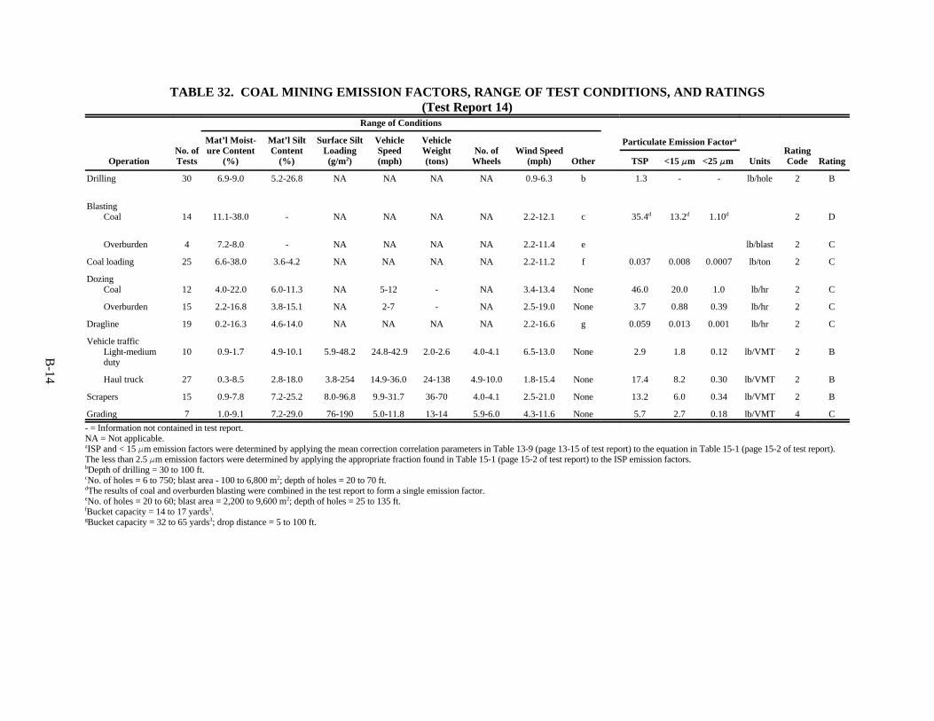
B-14
TABLE 32. COAL MINING EMISSION FACTORS, RANGE OF TEST CONDITIONS, AND RATINGS(Test Report 14)
OperationNo. ofTests
Range of Conditions
Particulate Emission Factora
UnitsRatingCode Rating
Mat’l Moist-ure Content
(%)
Mat’l SiltContent
(%)
Surface SiltLoading(g/m2)
VehicleSpeed(mph)
VehicleWeight(tons)
No. ofWheels
Wind Speed(mph) Other TSP <15 FFm <25 FFm
Drilling 30 6.9-9.0 5.2-26.8 NA NA NA NA 0.9-6.3 b 1.3 - - lb/hole 2 B
BlastingCoal 14 11.1-38.0 - NA NA NA NA 2.2-12.1 c 35.4d 13.2d 1.10d 2 D
Overburden 4 7.2-8.0 - NA NA NA NA 2.2-11.4 e lb/blast 2 C
Coal loading 25 6.6-38.0 3.6-4.2 NA NA NA NA 2.2-11.2 f 0.037 0.008 0.0007 lb/ton 2 C
DozingCoal 12 4.0-22.0 6.0-11.3 NA 5-12 - NA 3.4-13.4 None 46.0 20.0 1.0 lb/hr 2 C
Overburden 15 2.2-16.8 3.8-15.1 NA 2-7 - NA 2.5-19.0 None 3.7 0.88 0.39 lb/hr 2 C
Dragline 19 0.2-16.3 4.6-14.0 NA NA NA NA 2.2-16.6 g 0.059 0.013 0.001 lb/hr 2 C
Vehicle trafficLight-mediumduty
10 0.9-1.7 4.9-10.1 5.9-48.2 24.8-42.9 2.0-2.6 4.0-4.1 6.5-13.0 None 2.9 1.8 0.12 lb/VMT 2 B
Haul truck 27 0.3-8.5 2.8-18.0 3.8-254 14.9-36.0 24-138 4.9-10.0 1.8-15.4 None 17.4 8.2 0.30 lb/VMT 2 B
Scrapers 15 0.9-7.8 7.2-25.2 8.0-96.8 9.9-31.7 36-70 4.0-4.1 2.5-21.0 None 13.2 6.0 0.34 lb/VMT 2 B
Grading 7 1.0-9.1 7.2-29.0 76-190 5.0-11.8 13-14 5.9-6.0 4.3-11.6 None 5.7 2.7 0.18 lb/VMT 4 C
- = Information not contained in test report.NA = Not applicable.aISP and < 15 Fm emission factors were determined by applying the mean correction correlation parameters in Table 13-9 (page 13-15 of test report) to the equation in Table 15-1 (page 15-2 of test report).The less than 2.5 Fm emission factors were determined by applying the appropriate fraction found in Table 15-1 (page 15-2 of test report) to the ISP emission factors.bDepth of drilling = 30 to 100 ft.cNo. of holes = 6 to 750; blast area - 100 to 6,800 m2; depth of holes = 20 to 70 ft.dThe results of coal and overburden blasting were combined in the test report to form a single emission factor.eNo. of holes = 20 to 60; blast area = 2,200 to 9,600 m2; depth of holes = 25 to 135 ft.fBucket capacity = 14 to 17 yards3.gBucket capacity = 32 to 65 yards3; drop distance = 5 to 100 ft.
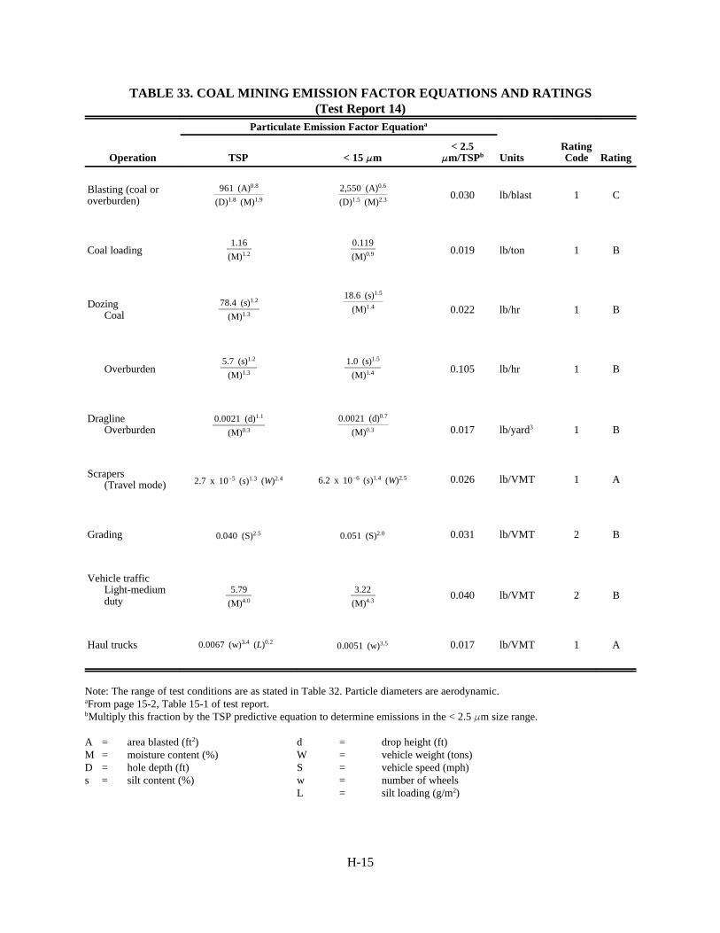
H-15
5.7 (s)1.2
(M)1.3
1.0 (s)1.5
(M)1.4
0.0021 (d)1.1
(M)0.3
0.0021 (d)0.7
(M)0.3
2.7 x 10&5 (s)1.3 (W)2.4 6.2 x 10&6 (s)1.4 (W)2.5
0.040 (S)2.5 0.051 (S)2.0
5.79
(M)4.0
3.22
(M)4.3
0.0067 (w)3.4 (L)0.2 0.0051 (w)3.5
TABLE 33. COAL MINING EMISSION FACTOR EQUATIONS AND RATINGS(Test Report 14)
Particulate Emission Factor Equationa
Operation TSP < 15 FFm< 2.5
FFm/TSPb UnitsRatingCode Rating
Blasting (coal oroverburden)
961 (A)0.8
(D)1.8 (M)1.9
2,550 (A)0.6
(D)1.5 (M)2.3 0.030 lb/blast 1 C
Coal loading1.16
(M)1.2
0.119
(M)0.9 0.019 lb/ton 1 B
DozingCoal
78.4 (s)1.2
(M)1.3
18.6 (s)1.5
(M)1.4 0.022 lb/hr 1 B
Overburden 0.105 lb/hr 1 B
DraglineOverburden 0.017 lb/yard3 1 B
Scrapers(Travel mode) 0.026 lb/VMT 1 A
Grading 0.031 lb/VMT 2 B
Vehicle trafficLight-mediumduty 0.040 lb/VMT 2 B
Haul trucks 0.017 lb/VMT 1 A
Note: The range of test conditions are as stated in Table 32. Particle diameters are aerodynamic.aFrom page 15-2, Table 15-1 of test report.bMultiply this fraction by the TSP predictive equation to determine emissions in the < 2.5 Fm size range.
A = area blasted (ft2) d = drop height (ft)M = moisture content (%) W = vehicle weight (tons)D = hole depth (ft) S = vehicle speed (mph)s = silt content (%) w = number of wheels
L = silt loading (g/m2)
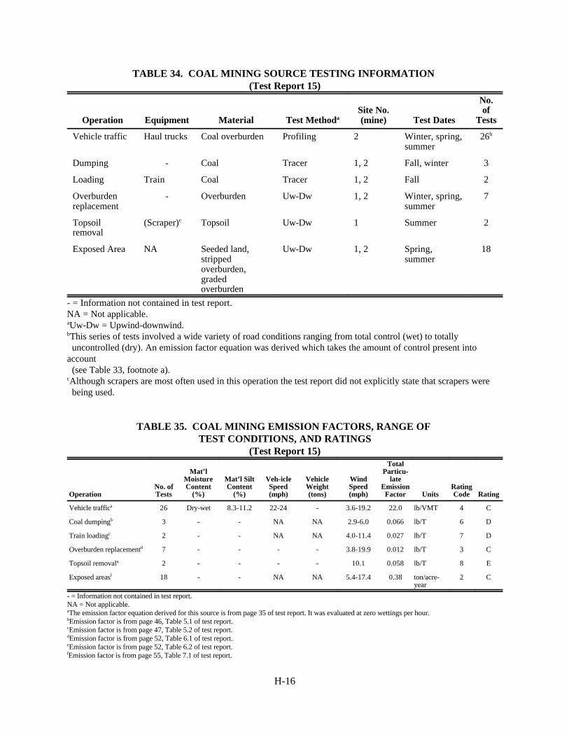
H-16
TABLE 34. COAL MINING SOURCE TESTING INFORMATION (Test Report 15)
Operation Equipment Material Test MethodaSite No.(mine) Test Dates
No.of
Tests
Vehicle traffic Haul trucks Coal overburden Profiling 2 Winter, spring,summer
26b
Dumping - Coal Tracer 1, 2 Fall, winter 3
Loading Train Coal Tracer 1, 2 Fall 2
Overburdenreplacement
- Overburden Uw-Dw 1, 2 Winter, spring,summer
7
Topsoilremoval
(Scraper)c Topsoil Uw-Dw 1 Summer 2
Exposed Area NA Seeded land,strippedoverburden,gradedoverburden
Uw-Dw 1, 2 Spring,summer
18
- = Information not contained in test report.NA = Not applicable.aUw-Dw = Upwind-downwind.bThis series of tests involved a wide variety of road conditions ranging from total control (wet) to totally uncontrolled (dry). An emission factor equation was derived which takes the amount of control present intoaccount (see Table 33, footnote a).cAlthough scrapers are most often used in this operation the test report did not explicitly state that scrapers were being used.
TABLE 35. COAL MINING EMISSION FACTORS, RANGE OF TEST CONDITIONS, AND RATINGS
(Test Report 15)
OperationNo. ofTests
Mat’lMoistureContent
(%)
Mat’l SiltContent
(%)
Veh-icleSpeed(mph)
VehicleWeight(tons)
WindSpeed(mph)
TotalParticu-
lateEmission
Factor UnitsRatingCode Rating
Vehicle traffica 26 Dry-wet 8.3-11.2 22-24 - 3.6-19.2 22.0 lb/VMT 4 C
Coal dumpingb 3 - - NA NA 2.9-6.0 0.066 lb/T 6 D
Train loadingc 2 - - NA NA 4.0-11.4 0.027 lb/T 7 D
Overburden replacementd 7 - - - - 3.8-19.9 0.012 lb/T 3 C
Topsoil removala 2 - - - - 10.1 0.058 lb/T 8 E
Exposed areasf 18 - - NA NA 5.4-17.4 0.38 ton/acre-year
2 C
- = Information not contained in test report.NA = Not applicable.aThe emission factor equation derived for this source is from page 35 of test report. It was evaluated at zero wettings per hour.bEmission factor is from page 46, Table 5.1 of test report.cEmission factor is from page 47, Table 5.2 of test report.dEmission factor is from page 52, Table 6.1 of test report.eEmission factor is from page 52, Table 6.2 of test report.fEmission factor is from page 55, Table 7.1 of test report.
H-17
8.5 Western Surface Coal Mining and Processing
Since no emission factors are currently presented in AP-42 for coal mining. The predictiveemission factor equations presented in Table 49 are recommended for inclusion in AP-42 under a sectionnamed "Western Surface Coal Mining." Table 50 presents the single-valued emission factors for westernsurface coal mining. It is recommended that for any source operation not covered by the equations in Table49, the highest rated singlevalued factors from Table 50 be incorporated in AP-42.
All of the recommended factors may be applied to Eastern surface coal mining. However, eachshould then be aerated one letter value (e.g., C to D).
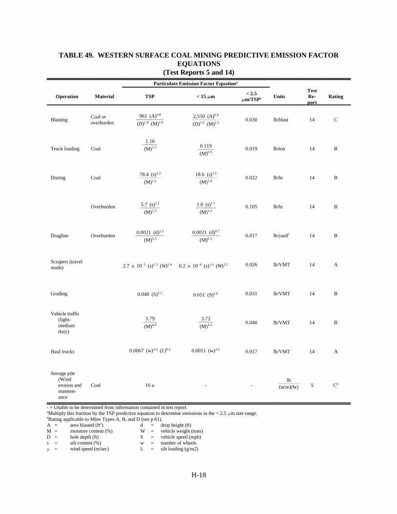
H-18
0.119
(M)0.9
78.4 (s)1.2
(M)1.3
18.6 (s)1.5
(M)1.4
5.7 (s)1.2
(M)1.3
1.0 (s)1.5
(M)1.4
0.0021 (d)1.1
(M)0.3
0.0021 (d)0.7
(M)0.3
2.7 x 10&5 (s)1.3 (W)2.4 6.2 x 10&6 (s)1.4 (W)2.5
0.040 (S)2.5 0.051 (S)2.0
5.79
(M)4.0
3.72
(M)4.3
0.0067 (w)3.4 (L)0.2 0.0051 (w)3.5
lb(acre)(hr)
TABLE 49. WESTERN SURFACE COAL MINING PREDICTIVE EMISSION FACTOREQUATIONS
(Test Reports 5 and 14)
Particulate Emission Factor Equationa
Operation Material TSP < 15 FFm< 2.5
FFm/TSPa UnitsTestRe-port
Rating
BlastingCoal oroverburden
961 (A)0.8
(D)1.8 (M)1.9
2,550 (A)0.6
(D)1.5 (M)2.30.030 lb/blast 14 C
Truck loading Coal
1.16
(M)1.2 0.019 lb/ton 14 B
Dozing Coal 0.022 lb/hr 14 B
Overburden 0.105 lb/hr 14 B
Dragline Overburden 0.017 lb/yard3 14 B
Scrapers (travelmode)
0.026 lb/VMT 14 A
Grading 0.031 lb/VMT 14 B
Vehicle traffic (light-
mediumduty)
0.040 lb/VMT 14 B
Haul trucks 0.017 lb/VMT 14 A
Storage pile(Winderosion andmainten-ance
Coal 16 u - - 5 Cb
- = Unable to be determined from information contained in test report.aMultiply this fraction by the TSP predictive equation to determine emissions in the < 2.5 Fm size range.bRating applicable to Mine Types A, B, and D (see p 61).A = area blasted (ft2) d = drop height (ft)M = moisture content (%) W = vehicle weight (tons)D = hole depth (ft) S = vehicle speed (mph)s = silt content (%) w = number of wheelsF = wind speed (m/sec) L = silt loading (g/m2)
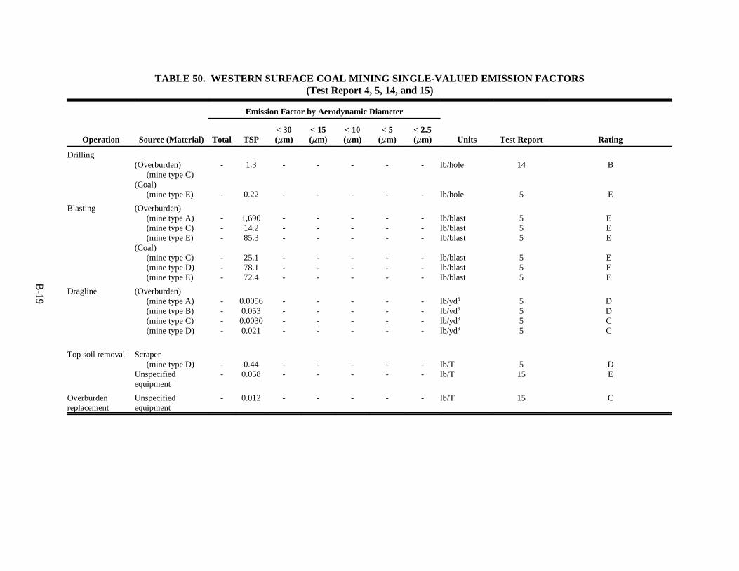
B-19
TABLE 50. WESTERN SURFACE COAL MINING SINGLE-VALUED EMISSION FACTORS(Test Report 4, 5, 14, and 15)
Emission Factor by Aerodynamic Diameter
Operation Source (Material) Total TSP< 30(FFm)
< 15(FFm)
< 10(FFm)
< 5(FFm)
< 2.5(FFm) Units Test Report Rating
Drilling(Overburden)
(mine type C)(Coal)
(mine type E)
-
-
1.3
0.22
-
-
-
-
-
-
-
-
-
-
lb/hole
lb/hole
14
5
B
E
Blasting (Overburden)(mine type A)(mine type C)(mine type E)
(Coal)(mine type C)(mine type D)(mine type E)
---
---
1,69014.285.3
25.178.172.4
---
---
---
---
---
---
---
---
---
---
lb/blastlb/blastlb/blast
lb/blastlb/blastlb/blast
555
555
E*E*E*
E*E*E*
Dragline (Overburden)(mine type A)(mine type B)(mine type C)(mine type D)
----
0.00560.0530.00300.021
----
----
----
----
----
lb/yd3
lb/yd3
lb/yd3
lb/yd3
5555
D*D*C*C*
Top soil removal Scraper(mine type D)
Unspecifiedequipment
--
0.440.058
--
--
--
--
--
lb/Tlb/T
515
DE
Overburdenreplacement
Unspecifiedequipment
- 0.012 - - - - - lb/T 15 C
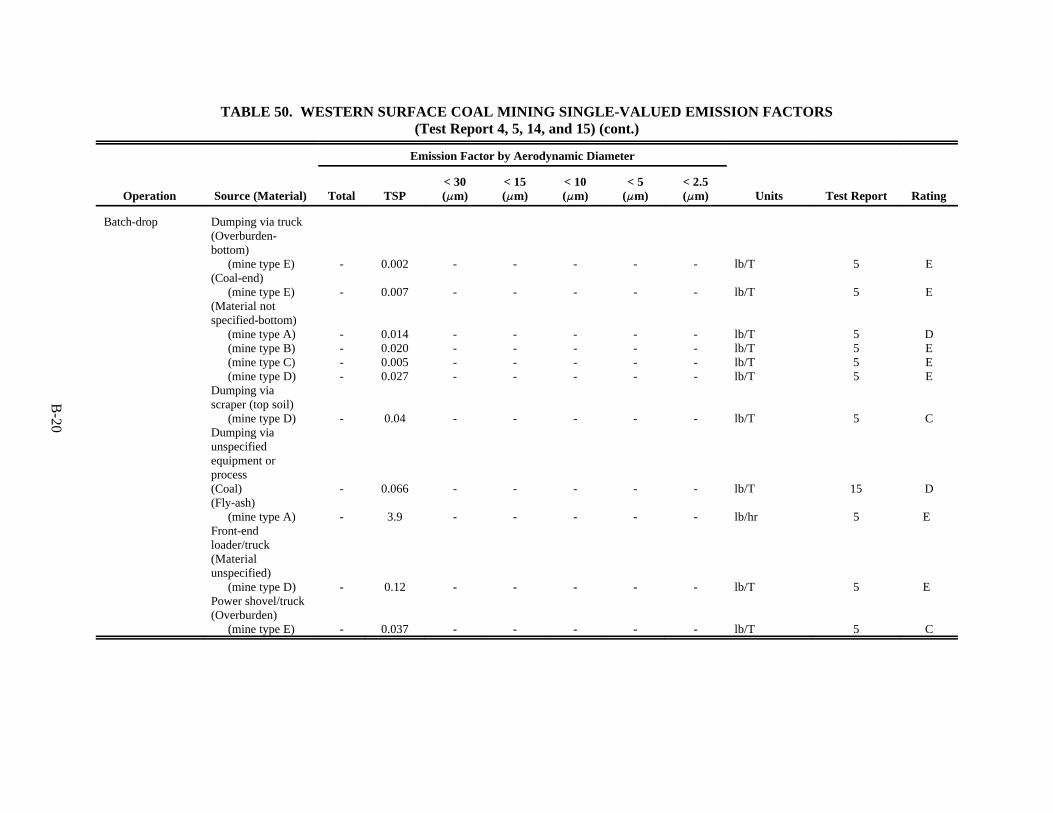
B-20
TABLE 50. WESTERN SURFACE COAL MINING SINGLE-VALUED EMISSION FACTORS(Test Report 4, 5, 14, and 15) (cont.)
Emission Factor by Aerodynamic Diameter
Operation Source (Material) Total TSP< 30(FFm)
< 15(FFm)
< 10(FFm)
< 5(FFm)
< 2.5(FFm) Units Test Report Rating
Batch-drop Dumping via truck(Overburden-bottom)
(mine type E)(Coal-end)
(mine type E)(Material notspecified-bottom)
(mine type A)(mine type B)(mine type C)(mine type D)
Dumping viascraper (top soil)
(mine type D)Dumping viaunspecifiedequipment orprocess(Coal)(Fly-ash)
(mine type A)Front-endloader/truck(Materialunspecified)
(mine type D)Power shovel/truck(Overburden)
(mine type E)
-
-
----
-
-
-
-
-
0.002
0.007
0.0140.0200.0050.027
0.04
0.066
3.9
0.12
0.037
-
-
----
-
-
-
-
-
-
-
----
-
-
-
-
-
-
-
----
-
-
-
-
-
-
-
----
-
-
-
-
-
-
-
----
-
-
-
-
-
lb/T
lb/T
lb/Tlb/Tlb/Tlb/T
lb/T
lb/T
lb/hr
lb/T
lb/T
5
5
5555
5
15
5
5
5
E
E
DEEE
C
D
E*
E*
C
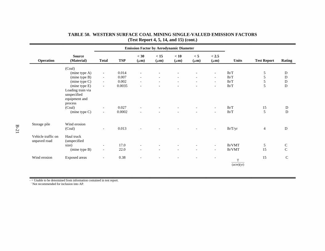
B-21
T(acre)(yr)
TABLE 50. WESTERN SURFACE COAL MINING SINGLE-VALUED EMISSION FACTORS(Test Report 4, 5, 14, and 15) (cont.)
Emission Factor by Aerodynamic Diameter
OperationSource
(Material) Total TSP< 30(FFm)
< 15(FFm)
< 10(FFm)
< 5(FFm)
< 2.5(FFm) Units Test Report Rating
(Coal)(mine type A)(mine type B)(mine type C)(mine type E)
Loading train viaunspecifiedequipment andprocess(Coal)
(mine type C)
----
--
0.0140.0070.0020.0035
0.0270.0002
----
--
----
--
----
--
----
--
----
--
lb/Tlb/Tlb/Tlb/T
lb/Tlb/T
5555
155
D*D*D*D*
DD
Storage pile Wind erosion(Coal) - 0.013 - - - - - lb/T/yr 4 D*
Vehicle traffic onunpaved road
Haul truck(unspecifiedsize)
(mine type B)--
17.022.0
--
--
--
--
--
lb/VMTlb/VMT
515
C*C*
Wind erosion Exposed areas - 0.38 - - - - - 15 C
- = Unable to be determined from information contained in test report.* = Not recommended for inclusion into AP.

H-22
H.2 Section 10 of EPA report "Improved Emission Factors For Fugitive Dust From Western SurfaceCoal Mining Sources --Volume I - Sampling Methodology and Test Results"
SECTION 10
RESULTS FOR SOURCES TESTED BY WIND TUNNEL METHOD
SUMMARY OF TESTS PERFORMED
As discussed previously, the wind tunnel method was used to test particulate emissions generatedby wind erosion of coal storage piles and exposed ground areas. These sources were tested at three minesites during the period October 1979 through August 1980.
A total of 37 successful wind tunnel tests were conducted at the three mines. Tests at Mine 1 tookplace in late autumn, with below normal temperatures and snowfall being encountered. Emissions testswere distributed by source and by mine as follows:
Number of Tests
Source Mine 1 Mine 2 Mine 3
Coal storage piles 4 7 16
Exposed ground piles 1 5 4
The decision of when to sample emissions from a given test surface was based on the first observation ofvisible emissions as the tunnel flow rate was increased. At Mines 1 and 2, if visible emissions in theblower exhaust were not observed at a particular tunnel flow rate, no air sampling was performed, but avelocity profile was obtained. Then the tunnel flow rate was increased to -he next level and the processrepeated. When visible emissions were observed, emission sampling was performed and then repeated atthe same wind speed (but for a longer sampling time) to measure the decay in the erosion rate. At Mine 3,particle movement on the test surface was used as the indicator that the threshold velocity had been reachedand that emission sampling should be performed. Five tests on coal piles and seven tests on exposedground areas were conducted on surfaces where no erosion was visually observed, and in these cases noemissions sampling was performed.
Table 10-1 lists the test site parameters for the wind tunnel tests conducted on coal pile surfaces. The ambient temperature and relative humidity measurements were obtained just above the coal surfaceexternal to the tunnel.
Table 10-2 gives the tunnel test conditions for the wind erosion emission tests on coal surfaces. The equivalent speed at 10 m was determined by extrapolation of the logarithmic velocity profile measuredin the wind tunnel test section above the eroding surface. The friction velocity, which is a measure of thewind shear at the eroding surface, was determined from the velocity profile.
Table 10-3 gives the erosion-related properties of the coal surfaces from which wind-generatedemissions were measured. The silt and moisture values were determined from laboratory analysis ofaggregate samples taken from representative undisturbed sections of the erodible surface ("before" erosion)and from the actual test surface after erosion; therefore, only one "before" condition and one "after"
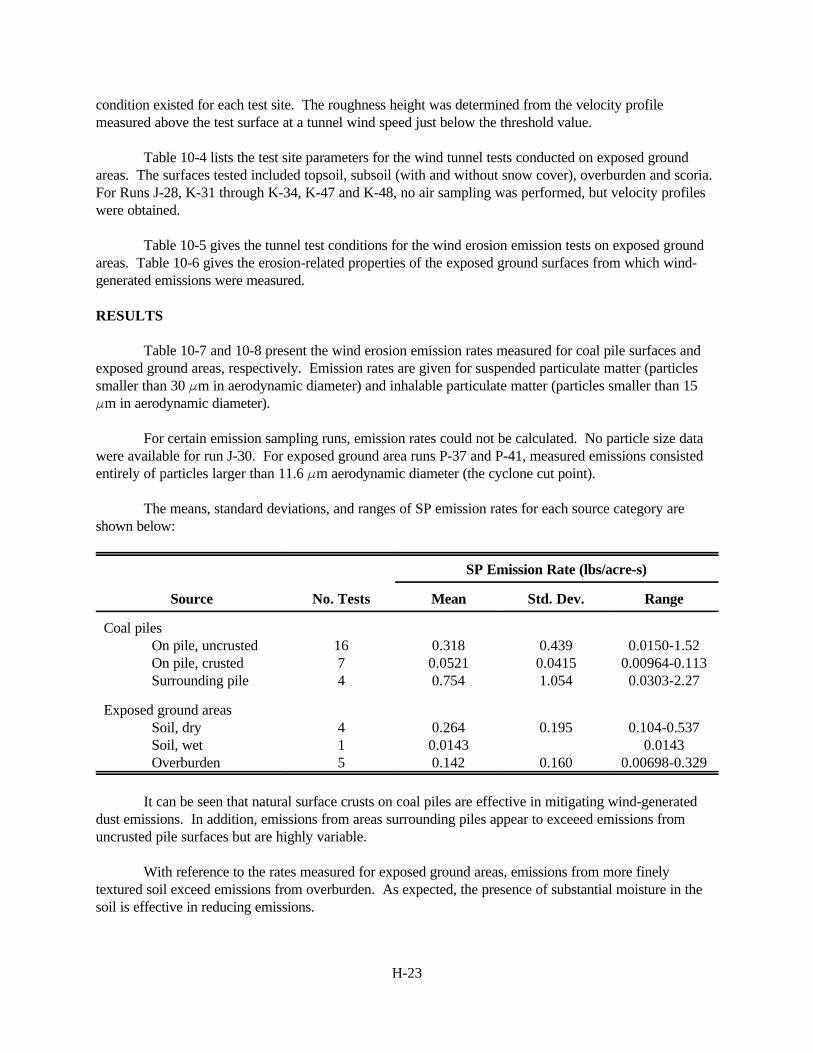
H-23
condition existed for each test site. The roughness height was determined from the velocity profilemeasured above the test surface at a tunnel wind speed just below the threshold value.
Table 10-4 lists the test site parameters for the wind tunnel tests conducted on exposed groundareas. The surfaces tested included topsoil, subsoil (with and without snow cover), overburden and scoria. For Runs J-28, K-31 through K-34, K-47 and K-48, no air sampling was performed, but velocity profileswere obtained.
Table 10-5 gives the tunnel test conditions for the wind erosion emission tests on exposed groundareas. Table 10-6 gives the erosion-related properties of the exposed ground surfaces from which wind-generated emissions were measured.
RESULTS
Table 10-7 and 10-8 present the wind erosion emission rates measured for coal pile surfaces andexposed ground areas, respectively. Emission rates are given for suspended particulate matter (particlessmaller than 30 Fm in aerodynamic diameter) and inhalable particulate matter (particles smaller than 15Fm in aerodynamic diameter).
For certain emission sampling runs, emission rates could not be calculated. No particle size datawere available for run J-30. For exposed ground area runs P-37 and P-41, measured emissions consistedentirely of particles larger than 11.6 Fm aerodynamic diameter (the cyclone cut point).
The means, standard deviations, and ranges of SP emission rates for each source category areshown below:
SP Emission Rate (lbs/acre-s)
Source No. Tests Mean Std. Dev. Range
Coal pilesOn pile, uncrustedOn pile, crustedSurrounding pile
1674
0.3180.05210.754
0.4390.04151.054
0.0150-1.520.00964-0.1130.0303-2.27
Exposed ground areasSoil, drySoil, wetOverburden
415
0.2640.01430.142
0.195
0.160
0.104-0.5370.0143
0.00698-0.329
It can be seen that natural surface crusts on coal piles are effective in mitigating wind-generateddust emissions. In addition, emissions from areas surrounding piles appear to exceeed emissions fromuncrusted pile surfaces but are highly variable.
With reference to the rates measured for exposed ground areas, emissions from more finelytextured soil exceed emissions from overburden. As expected, the presence of substantial moisture in thesoil is effective in reducing emissions.
H-24
Examination of the conditions under which tests were conducted indicates (1) an increase inemission rate with wind speed and (2) a decrease in emission rate with time after onset of erosion. Thismust be considered in comparing emission rates for different source conditions.
PROBLEMS ENCOUNTERED
The only significant problem in this phase of the study was the unforeseen resistnace of selectedtest surfaces to wind erosion. Threshold velocities were unexpectedly high and occasionally above themaximum tunnel wind speed. This occurred primarily because of the presence of natural surface crustswhich protected against erosion. As a result, the testing of many surfaces was limited to determination ofsurface roughness heights.
Although testing of emissions was intended to be restricted only to dry surfaces, the occurrence ofsnowfall at Mine 1 provided an interesting test condition for the effect of surface moisture. This helps tobetter quantify the seasonal variation in wind-generated emissions.
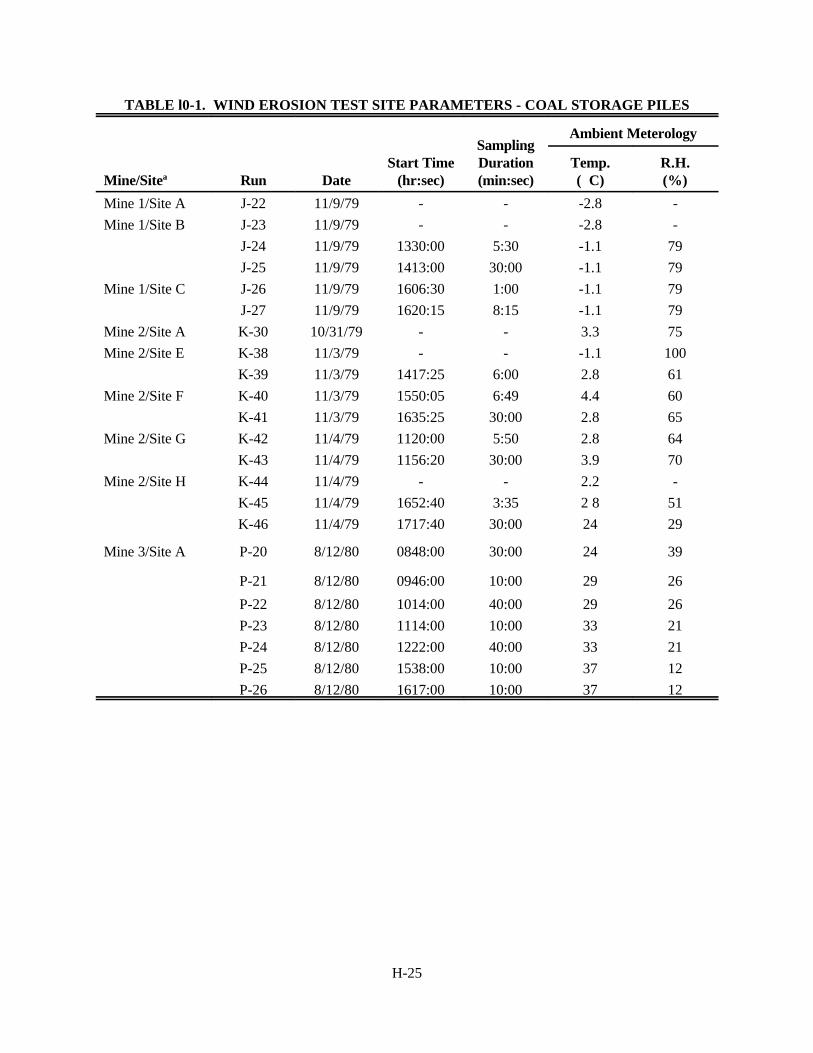
H-25
TABLE l0-1. WIND EROSION TEST SITE PARAMETERS - COAL STORAGE PILES
Mine/Sitea Run DateStart Time
(hr:sec)
SamplingDuration(min:sec)
Ambient Meterology
Temp.(EEC)
R.H.(%)
Mine 1/Site A J-22 11/9/79 - - -2.8 -
Mine 1/Site B J-23 11/9/79 - - -2.8 -
J-24 11/9/79 1330:00 5:30 -1.1 79
J-25 11/9/79 1413:00 30:00 -1.1 79
Mine 1/Site C J-26 11/9/79 1606:30 1:00 -1.1 79
J-27 11/9/79 1620:15 8:15 -1.1 79
Mine 2/Site A K-30 10/31/79 - - 3.3 75
Mine 2/Site E K-38 11/3/79 - - -1.1 100
K-39 11/3/79 1417:25 6:00 2.8 61
Mine 2/Site F K-40 11/3/79 1550:05 6:49 4.4 60
K-41 11/3/79 1635:25 30:00 2.8 65
Mine 2/Site G K-42 11/4/79 1120:00 5:50 2.8 64
K-43 11/4/79 1156:20 30:00 3.9 70
Mine 2/Site H K-44 11/4/79 - - 2.2 -
K-45 11/4/79 1652:40 3:35 2 8 51
K-46 11/4/79 1717:40 30:00 24 29
Mine 3/Site A P-20 8/12/80 0848:00 30:00 24 39
P-21 8/12/80 0946:00 10:00 29 26
P-22 8/12/80 1014:00 40:00 29 26
P-23 8/12/80 1114:00 10:00 33 21
P-24 8/12/80 1222:00 40:00 33 21
P-25 8/12/80 1538:00 10:00 37 12
P-26 8/12/80 1617:00 10:00 37 12
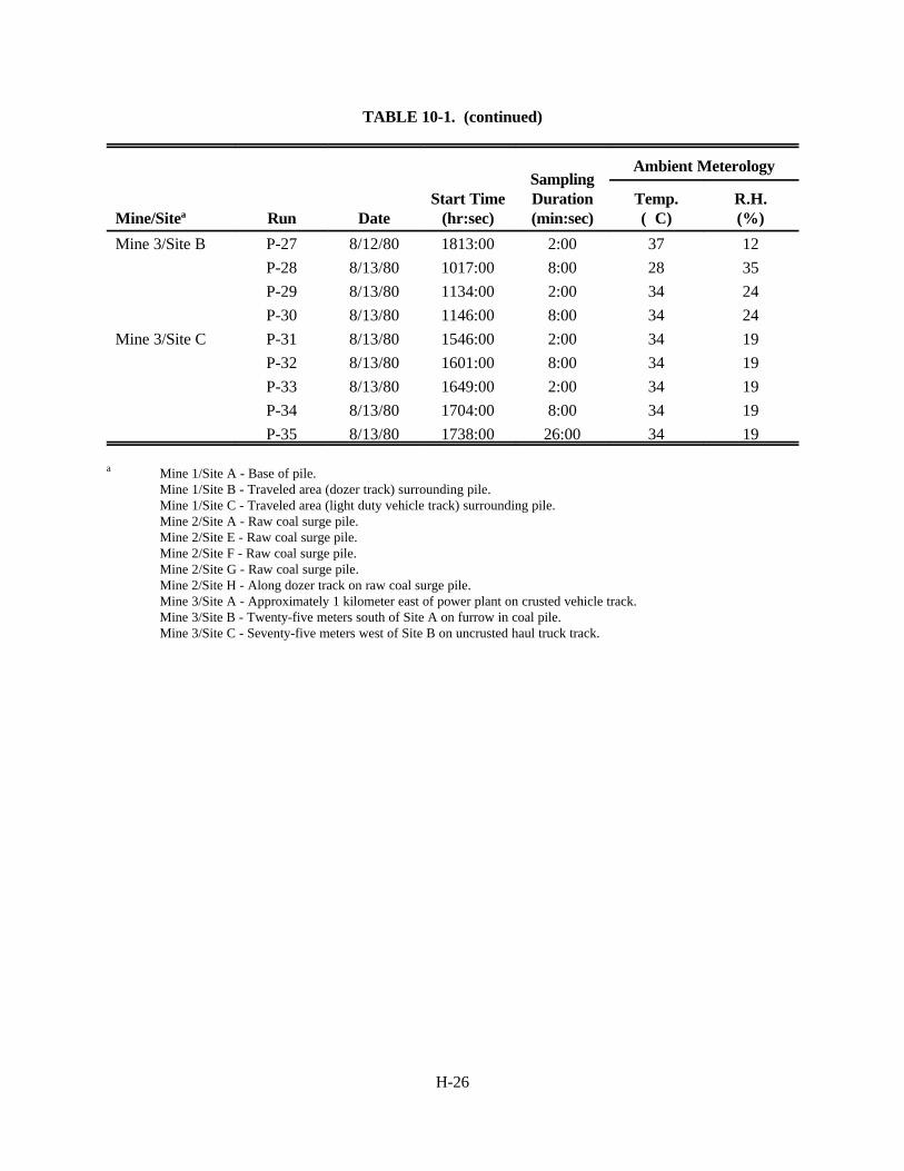
TABLE 10-1. (continued)
Mine/Sitea Run DateStart Time
(hr:sec)
SamplingDuration(min:sec)
Ambient Meterology
Temp.(EEC)
R.H.(%)
H-26
Mine 3/Site B P-27 8/12/80 1813:00 2:00 37 12
P-28 8/13/80 1017:00 8:00 28 35
P-29 8/13/80 1134:00 2:00 34 24
P-30 8/13/80 1146:00 8:00 34 24
Mine 3/Site C P-31 8/13/80 1546:00 2:00 34 19
P-32 8/13/80 1601:00 8:00 34 19
P-33 8/13/80 1649:00 2:00 34 19
P-34 8/13/80 1704:00 8:00 34 19
P-35 8/13/80 1738:00 26:00 34 19
a Mine 1/Site A - Base of pile.Mine 1/Site B - Traveled area (dozer track) surrounding pile.Mine 1/Site C - Traveled area (light duty vehicle track) surrounding pile.Mine 2/Site A - Raw coal surge pile.Mine 2/Site E - Raw coal surge pile.Mine 2/Site F - Raw coal surge pile.Mine 2/Site G - Raw coal surge pile.Mine 2/Site H - Along dozer track on raw coal surge pile.Mine 3/Site A - Approximately 1 kilometer east of power plant on crusted vehicle track.Mine 3/Site B - Twenty-five meters south of Site A on furrow in coal pile.Mine 3/Site C - Seventy-five meters west of Site B on uncrusted haul truck track.
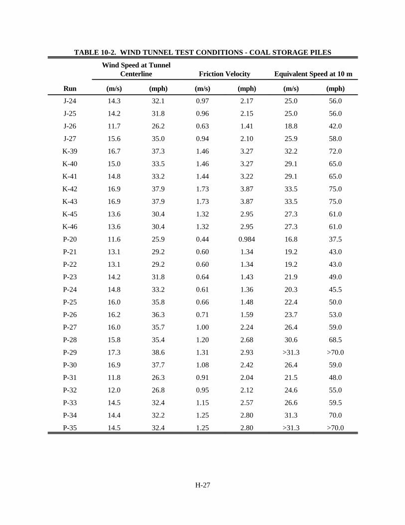
H-27
TABLE 10-2. WIND TUNNEL TEST CONDITIONS - COAL STORAGE PILES
Run
Wind Speed at TunnelCenterline Friction Velocity Equivalent Speed at 10 m
(m/s) (mph) (m/s) (mph) (m/s) (mph)
J-24 14.3 32.1 0.97 2.17 25.0 56.0
J-25 14.2 31.8 0.96 2.15 25.0 56.0
J-26 11.7 26.2 0.63 1.41 18.8 42.0
J-27 15.6 35.0 0.94 2.10 25.9 58.0
K-39 16.7 37.3 1.46 3.27 32.2 72.0
K-40 15.0 33.5 1.46 3.27 29.1 65.0
K-41 14.8 33.2 1.44 3.22 29.1 65.0
K-42 16.9 37.9 1.73 3.87 33.5 75.0
K-43 16.9 37.9 1.73 3.87 33.5 75.0
K-45 13.6 30.4 1.32 2.95 27.3 61.0
K-46 13.6 30.4 1.32 2.95 27.3 61.0
P-20 11.6 25.9 0.44 0.984 16.8 37.5
P-21 13.1 29.2 0.60 1.34 19.2 43.0
P-22 13.1 29.2 0.60 1.34 19.2 43.0
P-23 14.2 31.8 0.64 1.43 21.9 49.0
P-24 14.8 33.2 0.61 1.36 20.3 45.5
P-25 16.0 35.8 0.66 1.48 22.4 50.0
P-26 16.2 36.3 0.71 1.59 23.7 53.0
P-27 16.0 35.7 1.00 2.24 26.4 59.0
P-28 15.8 35.4 1.20 2.68 30.6 68.5
P-29 17.3 38.6 1.31 2.93 >31.3 >70.0
P-30 16.9 37.7 1.08 2.42 26.4 59.0
P-31 11.8 26.3 0.91 2.04 21.5 48.0
P-32 12.0 26.8 0.95 2.12 24.6 55.0
P-33 14.5 32.4 1.15 2.57 26.6 59.5
P-34 14.4 32.2 1.25 2.80 31.3 70.0
P-35 14.5 32.4 1.25 2.80 >31.3 >70.0
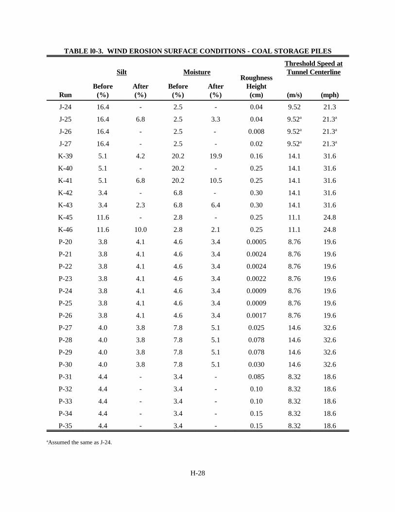
H-28
TABLE l0-3. WIND EROSION SURFACE CONDITIONS - COAL STORAGE PILES
Run
Silt MoistureRoughness
Height(cm)
Threshold Speed atTunnel Centerline
Before(%)
After(%)
Before(%)
After(%) (m/s) (mph)
J-24 16.4 - 2.5 - 0.04 9.52 21.3
J-25 16.4 6.8 2.5 3.3 0.04 9.52a 21.3a
J-26 16.4 - 2.5 - 0.008 9.52a 21.3a
J-27 16.4 - 2.5 - 0.02 9.52a 21.3a
K-39 5.1 4.2 20.2 19.9 0.16 14.1 31.6
K-40 5.1 - 20.2 - 0.25 14.1 31.6
K-41 5.1 6.8 20.2 10.5 0.25 14.1 31.6
K-42 3.4 - 6.8 - 0.30 14.1 31.6
K-43 3.4 2.3 6.8 6.4 0.30 14.1 31.6
K-45 11.6 - 2.8 - 0.25 11.1 24.8
K-46 11.6 10.0 2.8 2.1 0.25 11.1 24.8
P-20 3.8 4.1 4.6 3.4 0.0005 8.76 19.6
P-21 3.8 4.1 4.6 3.4 0.0024 8.76 19.6
P-22 3.8 4.1 4.6 3.4 0.0024 8.76 19.6
P-23 3.8 4.1 4.6 3.4 0.0022 8.76 19.6
P-24 3.8 4.1 4.6 3.4 0.0009 8.76 19.6
P-25 3.8 4.1 4.6 3.4 0.0009 8.76 19.6
P-26 3.8 4.1 4.6 3.4 0.0017 8.76 19.6
P-27 4.0 3.8 7.8 5.1 0.025 14.6 32.6
P-28 4.0 3.8 7.8 5.1 0.078 14.6 32.6
P-29 4.0 3.8 7.8 5.1 0.078 14.6 32.6
P-30 4.0 3.8 7.8 5.1 0.030 14.6 32.6
P-31 4.4 - 3.4 - 0.085 8.32 18.6
P-32 4.4 - 3.4 - 0.10 8.32 18.6
P-33 4.4 - 3.4 - 0.10 8.32 18.6
P-34 4.4 - 3.4 - 0.15 8.32 18.6
P-35 4.4 - 3.4 - 0.15 8.32 18.6
aAssumed the same as J-24.
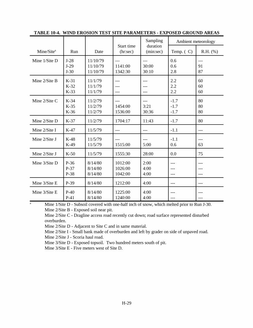
H-29
TABLE 10-4. WIND EROSION TEST SITE PARAMETERS - EXPOSED GROUND AREAS
Mine/Sitea Run DateStart time(hr:sec)
Samplingduration(min:sec)
Ambient meteorology
Temp. (EC) R.H. (%)
Mine 1/Site D J-28J-29J-30
11/10/7911/10/7911/10/79
---1141:001342:30
---30:0030:10
0.60.62.8
---9187
Mine 2/Site B K-31K-32K-33
11/1/7911/1/7911/1/79
---------
---------
2.22.22.2
606060
Mine 2/Site C K-34K-35K-36
11/2/7911/2/7911/2/79
---1454:001536:00
---3:2130:36
-1.7-1.7-1.7
808080
Mine 2/Site D K-37 11/2/79 1704:17 11:43 -1.7 80
Mine 2/Site I K-47 11/5/79 --- --- -1.1 ---
Mine 2/Site J K-48K-49
11/5/7911/5/79
---1515:00
---5:00
-1.10.6
---63
Mine 2/Site J K-50 11/5/79 1555:30 28:00 0.0 75
Mine 3/Site D P-36P-37P-38
8/14/808/14/808/14/80
1012:001026:001042:00
2:004:004:00
---------
---------
Mine 3/Site E P-39 8/14/80 1212:00 4:00 --- ---
Mine 3/Site E P-40P-41
8/14/808/14/80
1225:001240:00
4:004:00
------
------
a Mine 1/Site D - Subsoil covered with one-half inch of snow, which melted prior to Run J-30.Mine 2/Site B - Exposed soil near pit.Mine 2/Site C - Dragline access road recently cut down; road surface represented disturbedoverburden.Mine 2/Site D - Adjacent to Site C and in same material.Mine 2/Site I - Small bank made of overburden and left by grader on side of unpaved road.Mine 2/Site J - Scoria haul road.Mine 3/Site D - Exposed topsoil. Two hundred meters south of pit.Mine 3/Site E - Five meters west of Site D.

H-30
TABLE 10-5. WIND TUNNEL TEST CONDITIONS - EXPOSED GROUND AREAS
Run
Wind speed attunnel centerline Friction velocity
Equivalent speedat 10 m
(m/s) (mph) (m/s) (mph) (m/s) (mph)
J-29 18.1 40.5 1.96 4.38 38.0 85.0
J-30 16.6 37.1 1.62 3.62 32.6 73.0
K-35 15.1 33.7 1.54 3.44 30.9 69.0
K-36 14.8 33.1 1.51 3.38 30.0 67.0
K-37 15.1 33.7 1.54 3.44 30.9 69.0
K-49 15.8 35.4 1.56 3.49 30.4 68.0
K-50 15.8 35.4 1.56 3.49 30.4 68.0
P-36 10.3 19.6 0.87 1.95 15.7 35.0
P-37 10.3 19.6 0.87 1.95 15.7 35.0
P-38 10.3 19.6 0.87 1.95 15.7 35.0
P-39 6.3 14.0 0.33 0.738 10.3 23.0
P-40 8.1 18.0 0.44 0.984 13.0 29.0
P-41 10.7 23.9 1.00 2.24 20.1 45.0

H-31
TABLE 10-6. WIND EROSION SURFACE CONDITION - EXPOSED GROUND AREAS
Run
Silt Moisture RoughnessHeight(cm)
Threshold speed attunnel centerline
Before (%) After (%) Before (%) After (%) (ms/) (mph)
J-29 -- -- -- -- 0.38 >18.3 >41
J-30 -- -- -- -- 0.25 >18.3 >41
K-35 21.1 18.8 6.4 5.6 0.30 10.5 23.4
K-36 21.1 18.8 6.4 5.6 0.30 10.5 23.4
K-37 21.1 22.7 6.4 5.6 0.30 10.5 23.4
K-49 18.8 -- 4.1 -- 0.26 13.5 30.1
K-50 18.8 15.1 4.1 2.7 0.26 13.5 30.1
P-36 5.1 -- 0.8 -- 0.13 4.65 10.4
P-37 5.1 -- 0.8 -- 0.13 4.65 10.4
P-38 5.1 -- 0.8 -- 0.13 4.65 10.4
P-39 5.1 -- -- -- 0.0075 5.14 11.5
P-40 5.1 -- -- -- 0.01 5.14 11.5
P-41 5.1 -- -- -- 0.21 5.14 11.5

H-32
TABLE 10-7. WIND EROSION TEST RESULTS - COAL STORAGE PILES
Emission Rate
Suspended Particulate Inhalable Particulate
(g/m2-s) (lb/acre-s) (g/m2-s) (lb/acre-s)
J-24 0.00340 0.0303 0.00226 0.0202
J-25 0.00520 0.0464 0.00344 0.0307
J-26 0.254 2.27 0.157 1.40
J-27 0.0748 0.668 0.0472 0.421
K-39 0.170 1.52 0.119 1.06
K-40 0.111 0.991 0.0722 0.644
K-41 0.00454 0.0405 0.00296 0.0264
K-42 0.0961 0.831 0.0626 0.559
K-43 0.00436 0.0389 0.00279 0.0249
K-45 0.0598 0.534 0.0436 0.389
K-46 0.00741 0.0661 0.00548 0.0489
P-20 0.0127 0.113 0.00811 0.0724
P-21 0.00966 0.0862 0.00414 0.0369
P-22 0.00108 0.00964 0.000597 0.00533
P-23 0.00232 0.0207 0.00139 0.0124
P-24 0.00176 0.0157 0.00107 0.00955
P-25 0.00392 0.0350 O.C0231 0.0206
P-26 0.00948 0.0846 0.00533 0.0476
P-27 0.0386 0.344 0.0202 0.180
P-28 0.00578 0.0516 0.00343 0.0306
P-29 0.0161 0.144 0.0112 0.100
P-30 0.00168 0.0150 0.000970 0.00866
P-31 0.0191 0.170 0.0101 0.0901
P-32 0.00231 0.0206 0.000943 0.00842
P-33 0.0274 0.245 0.0157 0.140
P-34 0.00605 0.0540 0.00303 0.0270
P-35 0.00278 0.0248 0.00185 0.0165
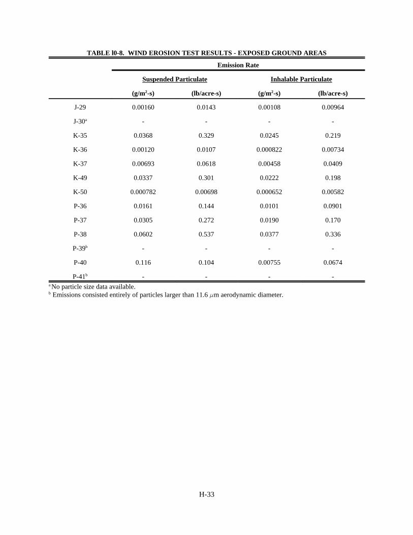
H-33
TABLE l0-8. WIND EROSION TEST RESULTS - EXPOSED GROUND AREAS
Emission Rate
Suspended Particulate Inhalable Particulate
(g/m2-s) (lb/acre-s) (g/m2-s) (lb/acre-s)
J-29 0.00160 0.0143 0.00108 0.00964
J-30a - - - -
K-35 0.0368 0.329 0.0245 0.219
K-36 0.00120 0.0107 0.000822 0.00734
K-37 0.00693 0.0618 0.00458 0.0409
K-49 0.0337 0.301 0.0222 0.198
K-50 0.000782 0.00698 0.000652 0.00582
P-36 0.0161 0.144 0.0101 0.0901
P-37 0.0305 0.272 0.0190 0.170
P-38 0.0602 0.537 0.0377 0.336
P-39b - - - -
P-40 0.116 0.104 0.00755 0.0674
P-41b - - - -a No particle size data available.b Emissions consisted entirely of particles larger than 11.6 Fm aerodynamic diameter.
I-1
Appendix IDevelopment of Correction Factors and Emission
Factor Equations
This appendix contains information on the development of correction factors and emission factor
equations for fugitive dust emissions. The information is from Sections 5 and 13, and Appendices A and B
of the EPA report “Improved Emission Factors For Fugitive Dust From Western Surface Coal Mining
Sources - Volume I and 11.”
I-2
TABLE OF CONTENTS
I.1 Sections 5 and 13, and Appendices A and B of the EPA report “Improved
Emission Factors For Fugitive Dust From Western Surface Coal Mining
Sources - Volume I and 11.” . . . . . . . . . . . . . . . . . . . . . . . . . . . . . . . . . . . . . . . . . . . . . . I-3
I-3
n't 2s 2
1
d 2(Eq.1)
SECTION 5
CALCULATION AND DATA ANALYSIS METHODOLOGY
NUMBER OF TESTS PER SOURCE
The study design proposed the number of samples to be collected for each operation, but these
initial numbers were based primarily on available sampling time and the relative importance of each
operation as a dust source. Several members of the technical review group requested a statistical analysis to
determine the appropriate number of samples to be taken.
After sampling data were obtained from the first two mines/three visits, the total sample size
needed to achieve a specified margin of error and confidence level could be calculated by knowing the
variability of the partial data set. This method of estimating required sample size, in which about half of the
preliminarily-estimated sample size is taken and its standard deviation is used to provide a final estimate of
sample size, is called the two-stage or Stein method. The two-stage method, along with two preliminary
data evaluations, constituted the statistical plan finally prepared for the study.
The steps in estimating total sample sizes and remaining samples in the statistical plan were:
1. Determine (by source) whether samples taken in different seasons and/or at different mines
were from the same population. If they were, total sample size could be calculated directly.
2. Evaluate potential correction factors. If samples were not from a single distribution, significant
correction factors could bring them into a single distribution. If they were from populations
with the same mean, correction factors could reduce the residual standard deviation.
3. Calculate required sample sizes using residual standard deviations.
4. Calculate remaining samples required to achieve the desired margin of error and confidence
level and recommend the number of samples for each source to be taken at the third mine.
Two-Stage Method for Estimating Sample Size
If samples are to be taken from a single normal population, the required total sample size can be
calculated with the following equation based on the two-stage sampling method (Natrella 1963):
where n = number of samples required for first and second stages combined
s1 = estimate of population standard deviation based on n1 samples
t = tabled t-value for risk % and nl-1degrees of freedom
d = margin of error in estimating population mean
* Another test, the x2 test for goodness of fit, may be more appropriate for determining whether data arefrom a population with a normal distribution, but it was not used in the original statistical plan.
I-4
The margin of error, d, and the risk, ", that the estimate of the mean will deviate from the
population mean by an amount d or greater are specified by the user. A relative error of 25 percent(d/x)
and a risk level of 20 percent have been specified for the calculations presented herein based on the
intended use for the results, the measurement errors involved in obtaining the samples, and the accuracy of
emission factors currently being used for other sources. Having specified d (or ) and ", the onlyd/x
additional value needed to calculate n for each source is the estimate of population standard deviation, s1
(or ), based on the partial sample obtained to date, nl. s1/x
Samples from the Same Normal Population
One important restriction on the use of Equation 1, as noted above, is that samples (from different
mines) must be from a single normal distribution. If average emission rates for a specific source at three
different mines are 2, 10, and 50 lb/ton, and the three samples have relatively low variability, the combined
data cannot be assumed to be normally distributed with a common mean. Regardless of how many samples
were taken at each mine, the data would be trimodally distributed.
Therefore, before Equation 1 can be used to calculate the total sample size, a check should be
performed to determine whether the available data from different mines are from populations with the same
mean and variance. If not, the mines would need to be treated separately and thus require a calculation of
required sample size for each mine, using the analogue of Equation 1 (n = number of samples at a single
mine). The total sample size would then be the total of the three sample sizes calculated for the respective
mines.
A statistical test can be performed on the data to evaluate whether two or more sets of samples
taken at different mines or in different seasons are from distributions (populations) having the same means
and variances (Natrella 1963; Hald 1952).* This test was performed in the statistical plan and indicated
that all sources at the first two mines/three visits except coal dozers, haul roads, and overburden drills were
from the same populations. Therefore, with the exceptions noted, total sample sizes could be determined
directly.
Correction Factors
The approach on which this study has been based is that the final emission factors will be mean
emission rates with correction factors attached to adequately account for the wide range of mining and
meteorological conditions over which the emission factors must be applied. The use of correction factors
may affect required sample sizes, in that correction factors which reduce the uncertainty (standard
deviation) in estimating an emission factor also reduce the sample size necessary to attain a desired
I-5
precision with a specified confidence. Therefore, the partial data from two mines were analyzed for
significant correction factors that could reduce the sample standard deviations and thus possibly reduce
required sample sizes. It should be pointed out that some additional samples are needed to adequately
quantify the effect of each correction factor on the emission factor, so a small reduction in sample size due
to the use of a correction factor would be offset by this need for extra data.
Independent variables thought to be candidates for correction factors were measured or monitored
with each sample of emission rate. The potential correction factors were listed in Table 3-5.
The approach for evaluation of correction factors described later in this section, multiple linear
regression, was used to identify significant correction factors in the partial data set. However, analysis was
not as thorough (e.g., did not include transformations) because it was being done only to get a slightly
better estimate of the optimum sample size.
The independent variables considered and their effects on standard deviation are summarized in
Table 5-1. Using appropriate values of s (standard deviation) in Equation 1, the sample sizes consistent
with the previously-discussed relative error of 25 percent and risk level of 20 percent were calculated.
These numbers are shown in Table 5-2, which was taken from the statistical plan. Some and s values inx
this table may not agree exactly with values reported later in the results sections because of minor changes
in calculation procedures between the time the statistical plan (e.g., method of extrapolating to 30 Fm SP
emission rate) was released and the final report was prepared.
These sample sizes were calculated after 2 mines/3 visits, leaving only one mine visit to obtain all
the additional samples. It was not possible to complete the sampling requirements specified in Table 5-2 at
the third mine within available project resources. Therefore, an attempt was made to get relative errors for
all sources down to 0.31 and major sources (haul trucks, scrapers, and draglines) down to 0.25 by slightly
reallocating the number of samples required for several of the sources. Table 5-3 compares four different
sets of sample sizes:
1. Originally proposed in study design.2. Calculated after 2 mines/3 visits to achieve a relative error of 25 percent at risk level of 0.20.3. Proposed in statistical plan as feasible totals after third mine.4. Actually collected at 3 mines/4 visits.
CALCULATION PROCEDURES
Exposure Profiling
To calculate emission rates using the exposure profiling technique, a conservation of mass
approach is used. The passage of airborne particulate, i.e., the quantity of emissions per unit of source
activity, is obtained by spatial integration of distributed measurements of exposure (mass/area) over the
effective cross section of the plume. The exposure is the point value of the flux (mass/area-time) of
I-6
cs'3.53x10⁴ mQst
(Eq. 3)
airborne particulate integrated over the time of measurement. The steps in the calculation procedure are
presented in the paragraphs below.
Step 1 Calculate Weights of Collected Sample--In order to calculate the total weight of particulate
matter collected by a sampler, the weights of air filters and of intake wash filters (profiler intakes and
cyclone precollectors only) are determined before and after use. The weight change of an unexposed filter
(blank) is used to adjust for the effects of filter handling. The following equation is used to calculate the
weight of particulate matter collected.
Particulate Final Tare Final Tare
sample = filter - filter - blank - blank (Eq. 2)
weight weight weight weight weight
Because of the typically small fractions of fines in fugitive dust plumes and the low sampling rate
of the dichotomous sampler, no weight gain may be detected on the fine filter of this instrument. This
makes it necessary to estimate a minimum detectable FP concentration corresponding to the minimum
weight gain which can be detected by the balance (0.005 mg). Since four individual tare and final weights
produce the particulate sample weight (Equation 2), the minimum detectable weight on a filter is 0.01 mg.
To calculate the minimum FP concentration, the sampling rate (1 m3/h) and duration of sampling
must be taken into account. For example, the minimum concentration which can be detected for a one-hour
sampling period is 10 Fg/m3. The actual sampling time should be used to calculate the minimum
concentration.
Step 2 Calculate Particulate Concentrations--The concentration of particulate matter measured by
a sampler, expressed in units of micrograms per standard cubic meter (Fg/som), is given by the following
equation:
where Cs = particulate concentration, Fg/scm
m = particulate sample weight, mg
Qs = sampler flow rate, SCFM
t = duration of sampling, min
I-7
{{
The coefficient in Equation 3 is simply a conversion factor. To be consistent with the National Ambient Air
Quality Standard for TSP, all concentrations are expressed in standard conditions (25°C and 29.92 in. of
Hg).
The specific particulate matter concentrations are determined from the various particulate catches
as follows:
Profiler: filter catch + intake catch
TP - or
Cyclone/cascade impactor: cyclone catch + substrate catches + backup
filter catch
TSP - Hi-vol sampler: filter catch
SP - Calculated: sub-30 Fm fraction determined by extrapolation of sub-2.5 and sub-15 Fm
fractions assuming a lognormal size distribution
IP - Size-selective inlet: filter catch
Dichotomous sampler: coarse particulate filter catch + fine particulate filter catch
FP - Dichotomous sampler: fine particle filter catch multiplied by 1.11
The dichotomous sampler total flow of l m3/h is divided into a coarse particle flow of 0.1 m3/h and a fine
particle flow of 0.9 m3/h. The mass collected on the fine particle filter is adjusted for fine particles which
remain in the air stream destined for the coarse particle filter.
Upwind (background) concentrations of TP or any of the respective size fractions are subtracted
from corresponding downwind concentrations to produce “net” concentrations attributable to the tested
source. Upwind sampling at one height (2.5 meters) did not allow determination of vertical variations of the
upwind concentration. Because the upwind concentration at 2.5 meters may be greater than at the 4 to 6
meter height of the downwind profiling tower, this may cause a downward bias of the net concentration.
Upwind TP is preferably obtained with an isokinetic sampler, but should be represented well by the upwind
TSP concentration measured by a standard hi-vol, if there are no nearby sources that would have a coarse
particle impact on the background station.
Step 3 Calculate Isokinetic Flow Ratios--The isokinetic flow ratio (IFR) is the ratio of the sampler
intake air speed to the wind speed approaching the sampler. It is given by:
I-8
IFR' QaU
'QS
aUs
(Eq. 4)
where Q = sampler flow rate, ACFM
Qs = sampler flow rate, SCFM
a = intake area of sampler, ft2
U = approaching wind speed, fpm
Us = approaching wind speed, sfpm
IFR is of interest in the sampling of TP, since isokinetic sampling assures that particles of all sizes are
sampled without bias.
Step 4 Calculate Downwind Particle Size Distributions--The downwind particle size distribution of
source-contributed particulate matter at a given height may be calculated from net TP, IP, and FP
concentrations at the same height (and distance from the source). Normally, the TP value from the
exposure profiler head would be used, unless a cascade impactor operates much closer to isokinetic
sampling conditions than the exposure profiler head.
The proper inlet cut-point of each dichotomous sampler must be determined based on the mean
wind speed at the height of the sampler. The concentration from a single upwind dichotomous sampler
should be adequately representative of the background contribution to the downwind dichotomous sampler
concentrations. The reasons are: (a) the background concentration should not vary appreciably with height;
(b) the upwind sampler, which is operated at an intermediate height, is exposed to a mean wind speed
which is within about 20 percent of the wind speed extremes that correspond to the range of downwind
sampler heights; and (c) errors resulting from the above conditions are small because of the typically small
contribution of background in comparison to the source plume.
Independent particle size distributions may be determined from a cascade impactor using the
proper 50 percent cutoff diameters for the cyclone precollector and each impaction stage. Corrections for
coarse particle bounce are recommended.
If it can be shown that the FP and apparent IP fractions of the net TP concentrations do not vary
significantly with height in the plume, i.e., by more than about 10 percent, then the plume can be
adequately characterized by a single particle size distribution. This size distribution is developed from the
dichotomous sampler net concentrations. The fine particle cutpoint of the dichotomous sampler (2.5 Fm)
corresponds to the midpoint of the normally observed bimodel size distribution of atmospheric aerosol. The
coarse mode represents particles produced by a single formation mechanism and can be expected to consist
of particles of lognormally distributed size. The best fit lognormal line through the data points (mass
I-9
' 3.05 x 10&8 CsUsT (Eq. 6)
E 'Ma
' 2.83 x 10&5CsQst
a(Eq. 5)
A ' mH
O
Edh (Eq. 7)
fractions of TP) is determined using a standard linear regression on transformed data points as described by
Reider and Cowherd (1979). This best fit line is extrapolated or interpolated to determine SP and IP
fractions of TP.
Step 5 Calculate Particulate Exposures and Integrate Profiles--For directional samplers operated
isokinetically, particulate exposures may be calculated by the following equation:
where E = particulate exposure, mg/cm2
M = net particulate mass collected by sampler, mg
a = sampler intake area, cm2
Cs = net particulate concentration, Fg/sm3
Us = approaching wind speed, sfpm
Qs = sampler flow rate, SCFM
t = duration of sampling, min
The coefficients of Equations 5 and 6 are conversion factors. Net mass or concentration refers to that
portion which is attributable to the source being tested, after subtraction of the contribution from
background.
Note that the above equations may also be written in terms of test parameters expressed in actual
rather than standard conditions. As mentioned earlier, the MRI profiler heads and warm-wire anemometers
give readings expressed at standard conditions.
The integrated exposure for a given particle size range is found by numerical integration of the
exposure profile over the height of the plume. Mathematically, this is stated as follows:
where A = integrated exposure, m-mg/cm2
E = particulate exposure, m-mg/cm2
h = vertical distance coordinate, m
H = effective extent of plume above ground, m
I-10
e ' 35.5 AN
(Eq. 8)
Physically, A represents the total passage of airborne particulate matter downwind of the source, per unit
length of line source.
The net exposure must equal zero at the vertical extremes of the profile, i.e., at the ground where
the wind velocity equals zero and at the effective height of the plume where the net concentration equals
zero. The maximum TP exposure usually occurs below a height of 1 m, so that there is a sharp decay in TP
exposure near the ground. The effective height of the plume is determined by extrapolation of the two
uppermost net TSP concentrations.
Integration of the portion of the net TP exposure profile that extends above a height of 1 m is
accomplished using Simpson's Rule on an odd number of equally spaced exposure values. The maximum
error in the integrated exposure resulting from extrapolation above the top sampler is estimated to be one-
half of the fraction of the plume mass which lies above the top sampler. The portion of the profile below a
height of 1 m is adequately depicted as a vertical line representing uniform exposure, because of the
offsetting effects of the usual occurrence of maximum exposure and the decay to zero exposure at ground
level (see Figure 5-1).
Step 6 Calculate Particulate Emission Rates--The TP emission rate for airborne particulate of a
given particle size range generated by vehicles traveling along a straight-line road segment, expressed in
pounds of emissions per vehicle-mile traveled (VMT), is given by:
where e = particulate emission rate, lb/VMT
A = integrated exposure, m-mg/cm2
N = number of vehicle passes, dimensionless
The coefficient of Equation 8 is simply a conversion factor. The metric equivalent emission rate is
expressed in kilograms (or grams) of particulate emissions per vehicle-kilometer traveled (VKT)
The SP, IP, and FP emission rates for a given test are calculated by multiplying the TP emission
rate by the respective size fractions obtained in Step 4.
Dustfall flux decays with distance downwind of the source, and the flux distribution may be
integrated to determine the portion of the TP emission which settles out near the source. Although this
effect has been analyzed in previous studies, it is not essential to the reduction of profiling data.
Consequently, no such analysis is being performed in the present study as part of the profiling calculations.
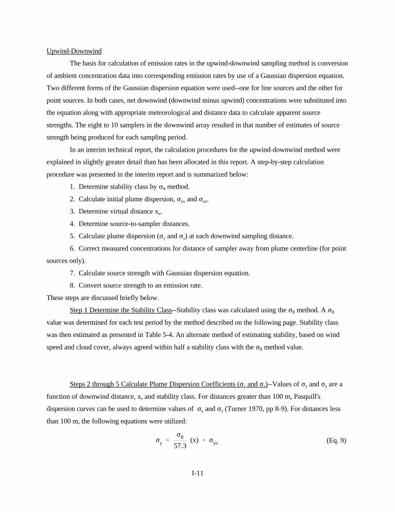
I-11
Fy 'F2
57.3(x) % Fyo (Eq. 9)
Upwind-Downwind
The basis for calculation of emission rates in the upwind-downwind sampling method is conversion
of ambient concentration data into corresponding emission rates by use of a Gaussian dispersion equation.
Two different forms of the Gaussian dispersion equation were used--one for line sources and the other for
point sources. In both cases, net downwind (downwind minus upwind) concentrations were substituted into
the equation along with appropriate meteorological and distance data to calculate apparent source
strengths. The eight to 10 samplers in the downwind array resulted in that number of estimates of source
strength being produced for each sampling period.
In an interim technical report, the calculation procedures for the upwind-downwind method were
explained in slightly greater detail than has been allocated in this report. A step-by-step calculation
procedure was presented in the interim report and is summarized below:
1. Determine stability class by F2 method.
2. Calculate initial plume dispersion, Fyo and Fzo.
3. Determine virtual distance xo.
4. Determine source-to-sampler distances.
5. Calculate plume dispersion (Fy and Fz) at each downwind sampling distance.
6. Correct measured concentrations for distance of sampler away from plume centerline (for point
sources only).
7. Calculate source strength with Gaussian dispersion equation.
8. Convert source strength to an emission rate.
These steps are discussed briefly below.
Step 1 Determine the Stability Class--Stability class was calculated using the F2 method. A F2
value was determined for each test period by the method described on the following page. Stability class
was then estimated as presented in Table 5-4. An alternate method of estimating stability, based on wind
speed and cloud cover, always agreed within half a stability class with the F2 method value.
Steps 2 through 5 Calculate Plume Dispersion Coefficients (Fy and Fz)--Values of Fy and Fz are a
function of downwind distance, x, and stability class. For distances greater than 100 m, Pasquill's
dispersion curves can be used to determine values of Fy and Fz (Turner 1970, pp 8-9). For distances less
than 100 m, the following equations were utilized:

I-12
Fz ' a(x % xo)b (Eq. 10)
xo 'b Fzo'a
The variables in Equations 9 and 10 were determined as follows:
F2 - The F2 value is the standard deviation of horizontal wind direction and was obtained by dividing
the wind direction strip chart recording for the test period into increments of 1 min each, specifying
an average direction for each increment, and calculating the standard deviation of the resulting set
of readings. The upper limit of F2 for use in Equation 18 is 32°.
P - The source-to-sampler distance was measured in the field and later obtained from the sketch of the
sampling setup for each test. It is the straight line distance from the source to the sampler rather
than the perpendicular distance from the source to a row of samplers.
Fyo - Initial horizontal plume dispersion is the initial plume width divided by 4.30 (Turner 1970). The
average initial plume width was observed and recorded during sampling. Photographs were also
taken.
a,b - These are empirically-derived dispersion coefficients that are only applicable within 100 m of a
ground-level source (Zimmerman and Thompson 1975). The coefficients are a function of stability
class:
Stability class a b
A 0.180 0.945
B 0.145 0.932
C 0.110 0.915
D 0.085 0.870
xo - The virtual distance term, xo, is used to simulate the effect of initial vertical plume dispersion. It is
estimated from the initial vertical plume dispersion value, Fzo, which in turn is the observed initial
plume height divided by 2.15 (Turner 1970):
Step 6 Correct Concentrations for Distance of Sampler Away from Plume Centerline--The
dispersion equations assume that sampling is done along the plume centerline. For line sources, this is a
reasonable assumption because the emissions occur at ground level and have an initial vertical dispersion
(Fzo) of 3 to 5 m. Therefore, the plume centerline is at about 2.5 m height, the same as the sampler heights.
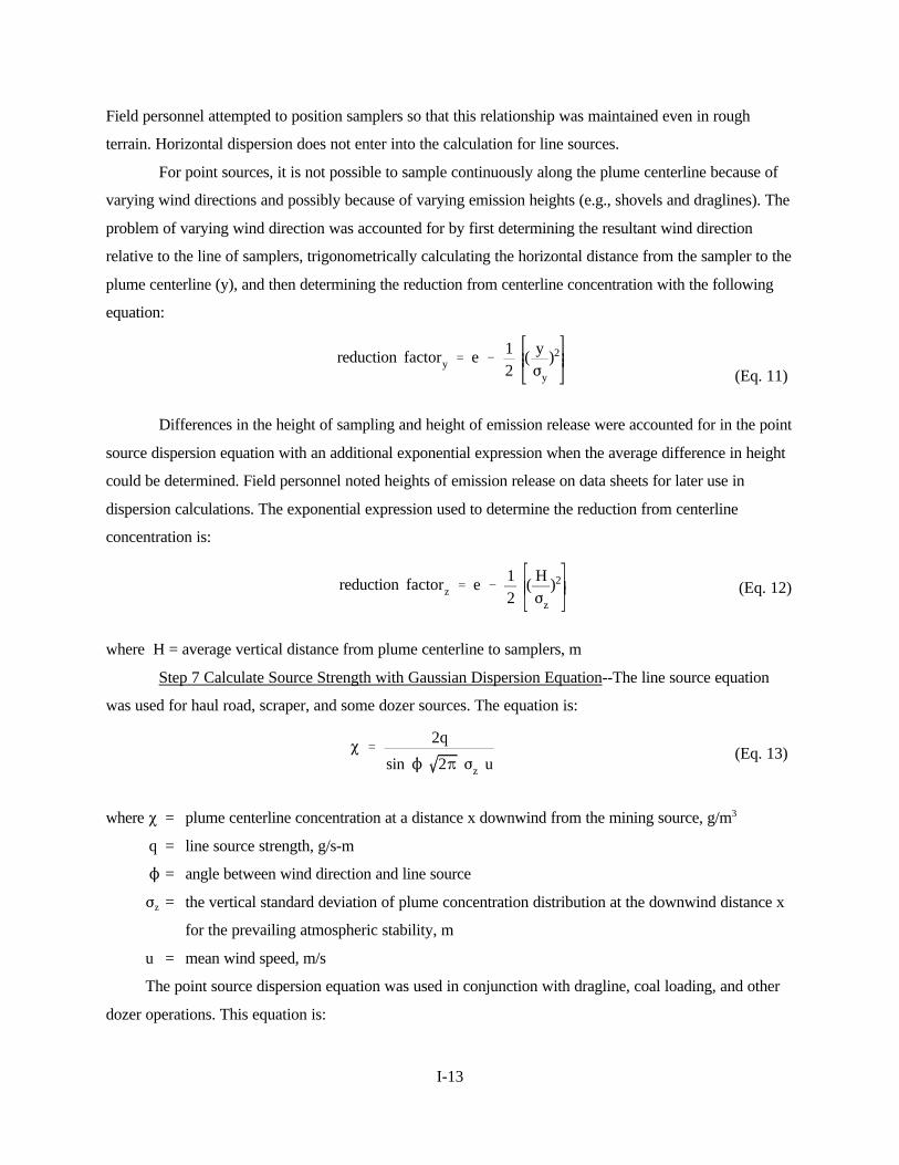
I-13
reduction factory ' e &12
( yFy
)2
(Eq. 11)
reduction factorz ' e &12
( HFz
)2(Eq. 12)
P '2q
sin N 2B Fz u(Eq. 13)
Field personnel attempted to position samplers so that this relationship was maintained even in rough
terrain. Horizontal dispersion does not enter into the calculation for line sources.
For point sources, it is not possible to sample continuously along the plume centerline because of
varying wind directions and possibly because of varying emission heights (e.g., shovels and draglines). The
problem of varying wind direction was accounted for by first determining the resultant wind direction
relative to the line of samplers, trigonometrically calculating the horizontal distance from the sampler to the
plume centerline (y), and then determining the reduction from centerline concentration with the following
equation:
Differences in the height of sampling and height of emission release were accounted for in the point
source dispersion equation with an additional exponential expression when the average difference in height
could be determined. Field personnel noted heights of emission release on data sheets for later use in
dispersion calculations. The exponential expression used to determine the reduction from centerline
concentration is:
where H = average vertical distance from plume centerline to samplers, m
Step 7 Calculate Source Strength with Gaussian Dispersion Equation--The line source equation
was used for haul road, scraper, and some dozer sources. The equation is:
where P = plume centerline concentration at a distance x downwind from the mining source, g/m3
q = line source strength, g/s-m
N = angle between wind direction and line source
Fz = the vertical standard deviation of plume concentration distribution at the downwind distance x
for the prevailing atmospheric stability, m
u = mean wind speed, m/s
The point source dispersion equation was used in conjunction with dragline, coal loading, and other
dozer operations. This equation is:
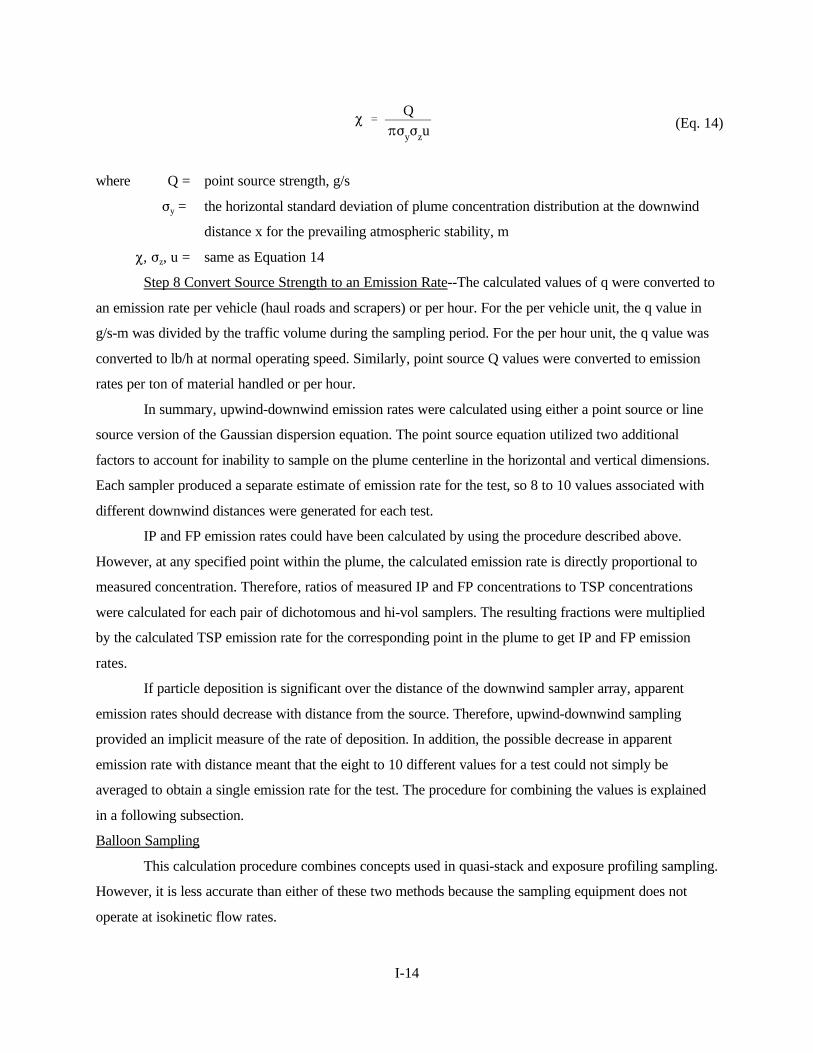
I-14
P 'Q
BFyFzu(Eq. 14)
where Q = point source strength, g/s
Fy = the horizontal standard deviation of plume concentration distribution at the downwind
distance x for the prevailing atmospheric stability, m
P, Fz, u = same as Equation 14
Step 8 Convert Source Strength to an Emission Rate--The calculated values of q were converted to
an emission rate per vehicle (haul roads and scrapers) or per hour. For the per vehicle unit, the q value in
g/s-m was divided by the traffic volume during the sampling period. For the per hour unit, the q value was
converted to lb/h at normal operating speed. Similarly, point source Q values were converted to emission
rates per ton of material handled or per hour.
In summary, upwind-downwind emission rates were calculated using either a point source or line
source version of the Gaussian dispersion equation. The point source equation utilized two additional
factors to account for inability to sample on the plume centerline in the horizontal and vertical dimensions.
Each sampler produced a separate estimate of emission rate for the test, so 8 to 10 values associated with
different downwind distances were generated for each test.
IP and FP emission rates could have been calculated by using the procedure described above.
However, at any specified point within the plume, the calculated emission rate is directly proportional to
measured concentration. Therefore, ratios of measured IP and FP concentrations to TSP concentrations
were calculated for each pair of dichotomous and hi-vol samplers. The resulting fractions were multiplied
by the calculated TSP emission rate for the corresponding point in the plume to get IP and FP emission
rates.
If particle deposition is significant over the distance of the downwind sampler array, apparent
emission rates should decrease with distance from the source. Therefore, upwind-downwind sampling
provided an implicit measure of the rate of deposition. In addition, the possible decrease in apparent
emission rate with distance meant that the eight to 10 different values for a test could not simply be
averaged to obtain a single emission rate for the test. The procedure for combining the values is explained
in a following subsection.
Balloon Sampling
This calculation procedure combines concepts used in quasi-stack and exposure profiling sampling.
However, it is less accurate than either of these two methods because the sampling equipment does not
operate at isokinetic flow rates.

I-15
E ' 60 V(u)t (Eq. 15)
The balloon samplers were preset to a flow rate that was isokinetic at a wind speed of 5 mph. Since
wind speed only approached this speed in two of the 18 tests, the sampling rates were normally super-
isokinetic. The other two types of equipment in the array, hi-vols and dichotomous samplers, sample at a
relatively constant air flow. In spite of this limitation, it was judged that a calculation involving integration
of concentrations would yield better results than could be obtained by using a dispersion equation.
Step 1. Plot Concentration Data in Horizontal and Vertical Dimensions--Concentration data from
the ground-based hi-vols and balloon-suspended samplers yield a concentration profile of the plume in both
the horizontal and vertical directions. By combining these profiles with visual observations and
photographs, it was possible to determine the plume boundaries. Conceptually, the next step was to
approximate the volume of air that passed the sampling array by multiplying the product of wind speed and
sampling duration by the cross-sectional area of the plume. This concept is similar to the procedures used
in the quasi-stack calculations. Quasi-stack calculations are discussed in the next subsection.
The calculation procedure is essentially a graphical integration technique. Concentrations measured
by the ground-level hi-vols (2.5 m height) were plotted against their horizontal spacing. By using visual
observations, photographs taken in the field, and the curve itself, the profile was extrapolated to zero
concentration at both edges of the plume. The resulting curve was assumed to represent the concentration
profile at ground level and was graphically integrated. This concept is demonstrated in Figure 5-2.
Step 2 Estimate the Volume Formed by the Two Profiles--The balloon samplers were suspended at
five specific heights of 2.5, 7.6, 15.2, 22.9, and 30.5 m. Since concentrations measured by these samplers
were not directly comparable to those from hi-vols, concentrations at the four heights above 2.5 m were
expressed as ratios of the 2.5 m concentration. The resulting curve of relative concentration versus height
was extrapolated to a height of zero concentration, as shown in Figure 5-3. The next step was to multiply
each of the ratios by the area under the ground-level concentration profile. This produced an approximation
of the relative integrated concentration at each of the five heights. By using a trapezoidal approximation
technique, an estimate of the volume formed by the two profiles was obtained.
Step 3 Calculate the TSP Emission Rate--The final emission rate calculation was made with the
following equation:
where E = total emissions from blast, mg
V = volume under the two profiles, mg/m
u = wind speed, m/s
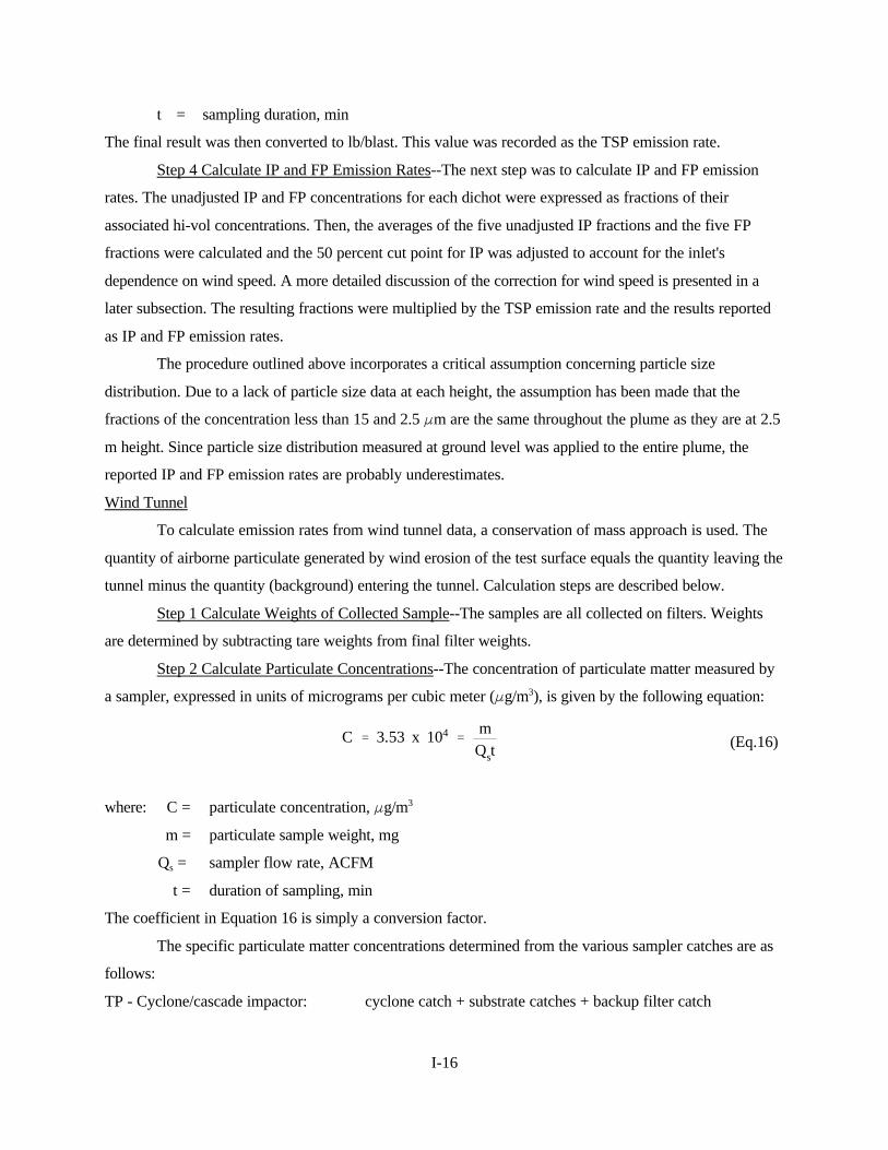
I-16
C ' 3.53 x 10⁴ 'm
Qst(Eq.16)
t = sampling duration, min
The final result was then converted to lb/blast. This value was recorded as the TSP emission rate.
Step 4 Calculate IP and FP Emission Rates--The next step was to calculate IP and FP emission
rates. The unadjusted IP and FP concentrations for each dichot were expressed as fractions of their
associated hi-vol concentrations. Then, the averages of the five unadjusted IP fractions and the five FP
fractions were calculated and the 50 percent cut point for IP was adjusted to account for the inlet's
dependence on wind speed. A more detailed discussion of the correction for wind speed is presented in a
later subsection. The resulting fractions were multiplied by the TSP emission rate and the results reported
as IP and FP emission rates.
The procedure outlined above incorporates a critical assumption concerning particle size
distribution. Due to a lack of particle size data at each height, the assumption has been made that the
fractions of the concentration less than 15 and 2.5 Fm are the same throughout the plume as they are at 2.5
m height. Since particle size distribution measured at ground level was applied to the entire plume, the
reported IP and FP emission rates are probably underestimates.
Wind Tunnel
To calculate emission rates from wind tunnel data, a conservation of mass approach is used. The
quantity of airborne particulate generated by wind erosion of the test surface equals the quantity leaving the
tunnel minus the quantity (background) entering the tunnel. Calculation steps are described below.
Step 1 Calculate Weights of Collected Sample--The samples are all collected on filters. Weights
are determined by subtracting tare weights from final filter weights.
Step 2 Calculate Particulate Concentrations--The concentration of particulate matter measured by
a sampler, expressed in units of micrograms per cubic meter (Fg/m3), is given by the following equation:
where: C = particulate concentration, Fg/m3
m = particulate sample weight, mg
Qs = sampler flow rate, ACFM
t = duration of sampling, min
The coefficient in Equation 16 is simply a conversion factor.
The specific particulate matter concentrations determined from the various sampler catches are as
follows:
TP - Cyclone/cascade impactor: cyclone catch + substrate catches + backup filter catch
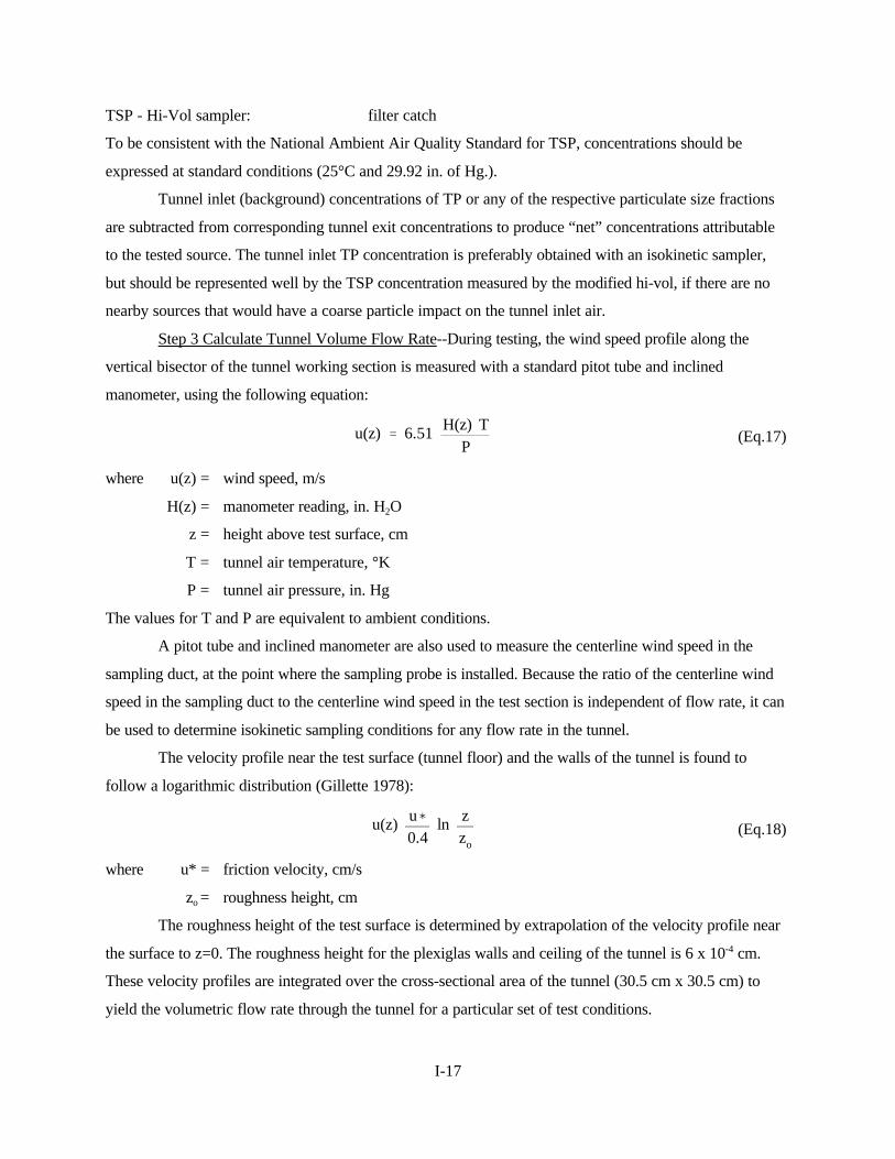
I-17
u(z) ' 6.51 H(z) TP
(Eq.17)
u(z) u(0.4
ln zzo
(Eq.18)
TSP - Hi-Vol sampler: filter catch
To be consistent with the National Ambient Air Quality Standard for TSP, concentrations should be
expressed at standard conditions (25°C and 29.92 in. of Hg.).
Tunnel inlet (background) concentrations of TP or any of the respective particulate size fractions
are subtracted from corresponding tunnel exit concentrations to produce “net” concentrations attributable
to the tested source. The tunnel inlet TP concentration is preferably obtained with an isokinetic sampler,
but should be represented well by the TSP concentration measured by the modified hi-vol, if there are no
nearby sources that would have a coarse particle impact on the tunnel inlet air.
Step 3 Calculate Tunnel Volume Flow Rate--During testing, the wind speed profile along the
vertical bisector of the tunnel working section is measured with a standard pitot tube and inclined
manometer, using the following equation:
where u(z) = wind speed, m/s
H(z) = manometer reading, in. H2O
z = height above test surface, cm
T = tunnel air temperature, °K
P = tunnel air pressure, in. Hg
The values for T and P are equivalent to ambient conditions.
A pitot tube and inclined manometer are also used to measure the centerline wind speed in the
sampling duct, at the point where the sampling probe is installed. Because the ratio of the centerline wind
speed in the sampling duct to the centerline wind speed in the test section is independent of flow rate, it can
be used to determine isokinetic sampling conditions for any flow rate in the tunnel.
The velocity profile near the test surface (tunnel floor) and the walls of the tunnel is found to
follow a logarithmic distribution (Gillette 1978):
where u* = friction velocity, cm/s
zo = roughness height, cm
The roughness height of the test surface is determined by extrapolation of the velocity profile near
the surface to z=0. The roughness height for the plexiglas walls and ceiling of the tunnel is 6 x 10⁻⁴ cm.
These velocity profiles are integrated over the cross-sectional area of the tunnel (30.5 cm x 30.5 cm) to
yield the volumetric flow rate through the tunnel for a particular set of test conditions.
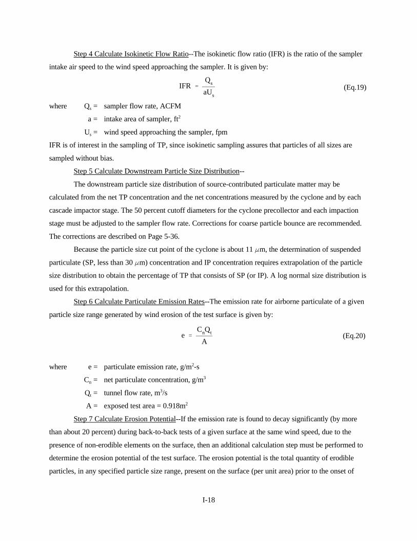
I-18
IFR 'Qs
aUs
(Eq.19)
e 'CnQt
A(Eq.20)
Step 4 Calculate Isokinetic Flow Ratio--The isokinetic flow ratio (IFR) is the ratio of the sampler
intake air speed to the wind speed approaching the sampler. It is given by:
where Qs = sampler flow rate, ACFM
a = intake area of sampler, ft2
Us = wind speed approaching the sampler, fpm
IFR is of interest in the sampling of TP, since isokinetic sampling assures that particles of all sizes are
sampled without bias.
Step 5 Calculate Downstream Particle Size Distribution--
The downstream particle size distribution of source-contributed particulate matter may be
calculated from the net TP concentration and the net concentrations measured by the cyclone and by each
cascade impactor stage. The 50 percent cutoff diameters for the cyclone precollector and each impaction
stage must be adjusted to the sampler flow rate. Corrections for coarse particle bounce are recommended.
The corrections are described on Page 5-36.
Because the particle size cut point of the cyclone is about 11 Fm, the determination of suspended
particulate (SP, less than 30 Fm) concentration and IP concentration requires extrapolation of the particle
size distribution to obtain the percentage of TP that consists of SP (or IP). A log normal size distribution is
used for this extrapolation.
Step 6 Calculate Particulate Emission Rates--The emission rate for airborne particulate of a given
particle size range generated by wind erosion of the test surface is given by:
where e = particulate emission rate, g/m2-s
Cn = net particulate concentration, g/m3
Qt = tunnel flow rate, m3/s
A = exposed test area = 0.918m2
Step 7 Calculate Erosion Potential--If the emission rate is found to decay significantly (by more
than about 20 percent) during back-to-back tests of a given surface at the same wind speed, due to the
presence of non-erodible elements on the surface, then an additional calculation step must be performed to
determine the erosion potential of the test surface. The erosion potential is the total quantity of erodible
particles, in any specified particle size range, present on the surface (per unit area) prior to the onset of

I-19
Mt ' Moe&kt (Eq. 21)
lnMo & L1
Mo
lnMo & L2
Mo
't1
t2
(Eq. 22)
E ' PV (Eq. 23)
erosion. Because wind erosion is an avalanching process, it is reasonable to assume that the loss rate from
the surface is proportional to the amount of erodible material remaining:
where Mt = quantity of erodible material present on the surface at any time, g/m2
Mo = erosion potential, i.e., quantity of erodible material present on the surface before the
onset of erosion, g/m2
k = constant, s-1
t = cumulative erosion time, s
Consistent with Equation 21, the erosion potential may be calculated from the measured losses
from the test surface for two erosion times:
where Ll = measured loss during time period 0 to tl, g/m2
L2 = measured loss during time period 0 to t2, g/m2
The loss may be back-calculated as the product of the emission rate from Equation 20 and the cumulative
erosion time.
Quasi-Stack
The source strengths of the drill tests are determined by multiplying the average particulate
concentration in the sampled volume of air by the total volume of air that passed through the enclosure
during the test. For this calculation procedure, the air passing through the enclosure is assumed to contain
all of the particulate emitted by the source. This calculation can be expressed as:
where E = source strength, g
P = concentration, g/m3
V = total volume, m3
Step 1 Determine Particle Size Fractions--As described in Section 3, isokinetic samplers were used
to obtain total concentration data for the particulate emissions passing through the enclosure. Originally,
these data were to be related to particle size, based on the results of microscopic analyses. However, the

I-20
Vi ' (ui) (a'4)(t) (Eq. 24)
E ' j4
i'1vi Pi (Eq. 25)
inconsistent results obtained from the comparability tests precluded the use of this technique for particle
sizing. Consequently, the total concentration data were divided into suspended and settleable fractions. The
filter fraction of the concentration was assumed to be suspended particulate and the remainder was
assumed to be settleable particulate.
Step 2 Determine Concentration for Each Sampler--Rather than traverse the enclosure, as is done
in conventional source testing, four separate profiler samplers were used during each test. These samplers
were spaced at regular intervals along the horizontal centerline of the enclosure. Each sampler was set to
the approximate isokinetic sampling rate. This rate was determined from the wind velocity measured at
each sampler with a hot-wire anemometer. The wind velocity was checked at each sampler every 2 to 3
minutes and the sampling rates were adjusted as necessary.
Step 3 Calculate Volume of Air Sampled by Each Profiler--In order to simplify the calculation of
source strength, it was assumed that the concentration and wind velocity measured at each sampler were
representative of one-fourth the cross-sectional area of the enclosure. Thus, the total volume of air
associated with each profiler concentration was calculated as follows:
where Vi = total volume of air associated with sampler i, m3
ui = mean velocity measured at sampler i, m/min
a = cross-sectional area of enclosure, m2
t = sampling duration, min
Step 4 Calculate the Total Emissions as Sum of Four Partial Emission Rates--Separate source
strengths, E, are calculated for the total concentration and the fraction captured on the filter. The equation
is:
These source strengths, in grams, were converted to pounds per hole drilled and are reported in Section 11.
PARTICLE SIZE CORRECTIONS
Several different size fraction measurements require a mathematical calculation to correct for some
deficiency in the sampling equipment from ideal size separation. Three of the calculation procedures are
described here:
Correction of dichotomous samples to 15 Fm values
Conversion of physical diameters measured microscopically to equivalent aerodynamic diameters
Correction of cascade impactor data to account for particle bounce-through.

I-21
Correction of Dichotomous Data
Recent research indicates that the collection efficiency of the dichotomous sampler inlet is
dependent on wind speed (Wedding 1980). As shown in Figure 5-4, the 50 percent cut point that is
nominally 15 Fm actually varies from 10 to 22 Fm over the range of wind speeds tested.
The procedure developed in the present study to correct dichot concentrations to a 15 Fm cut point
was to:
1. Determine the average wind speed for each test period.
2. Estimate the actual cut point for the sample from Figure 5-4.
3. Calculate net concentrations for each stage by subtracting upwind dichot concentrations.
4. Calculate the total concentration less than the estimated cut point diameter by summing the net
concentrations on the two stages.
5. Adjust the fine fraction (<2.5 Fm) concentration by multiplying by 1.11 to account for fine
particles that remain in the portion of the air stream that carries the coarse fraction particles.
6. Calculate the ratio of fine fraction to net TSP concentration and the ratio of total net dichot
concentration to net TSP concentration.
7. Plot (on log-probability paper) two data points on a graph of particle size versus fraction of
TSP concentration. The two points are the fraction less than 2.5 Fm and the fraction less than the cut point
determined in step 2.
8. Draw a straight line through the two points and interpolate or extrapolate the fraction less than
15 Fm. (Steps 7 and 8 are a graphical solution that may be replaced by a calculator program that can
perform the linear interpolation or extrapolation with greater precision.)
9. Calculate the net concentration less than 15 Fm from this fraction and the known net TSP
concentration.
A relatively small error is involved in the assumption of a log linear curve between the two points
because the 15 Fm point is so near the point for the actual upper limit particle size. The largest uncertainty
in applying this correction is probably the accuracy of the research data in Figure 5-4.
Conversion of Microscopy Data to Aerodynamic Diameters
Three calculation procedures for converting physical particle diameters into equivalent
aerodynamic diameters were found in the literature (Hesketh 1977; Stockham 1977; and Mercer 1973).
One of these was utilized in calculations in a recent EPA publication, so this procedure was adopted
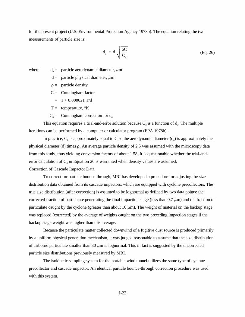
I-22
da ' d DCCa
(Eq. 26)
for the present project (U.S. Environmental Protection Agency 1978b). The equation relating the two
measurements of particle size is:
where da = particle aerodynamic diameter, Fm
d = particle physical diameter, Fm
D = particle density
C = Cunningham factor
= 1 + 0.000621 T/d
T = temperature, °K
Ca = Cunningham correction for da
This equation requires a trial-and-error solution because Ca is a function of da. The multiple
iterations can be performed by a computer or calculator program (EPA 1978b).
In practice, Ca is approximately equal to C so the aerodynamic diameter (da) is approximately the
physical diameter (d) times D. An average particle density of 2.5 was assumed with the microscopy data
from this study, thus yielding conversion factors of about 1.58. It is questionable whether the trial-and-
error calculation of Ca in Equation 26 is warranted when density values are assumed.
Correction of Cascade Impactor Data
To correct for particle bounce-through, MRI has developed a procedure for adjusting the size
distribution data obtained from its cascade impactors, which are equipped with cyclone precollectors. The
true size distribution (after correction) is assumed to be lognormal as defined by two data points: the
corrected fraction of particulate penetrating the final impaction stage (less than 0.7 Fm) and the fraction of
particulate caught by the cyclone (greater than about 10 Fm). The weight of material on the backup stage
was replaced (corrected) by the average of weights caught on the two preceding impaction stages if the
backup stage weight was higher than this average.
Because the particulate matter collected downwind of a fugitive dust source is produced primarily
by a uniform physical generation mechanism, it was judged reasonable to assume that the size distribution
of airborne particulate smaller than 30 Fm is lognormal. This in fact is suggested by the uncorrected
particle size distributions previously measured by MRI.
The isokinetic sampling system for the portable wind tunnel utilizes the same type of cyclone
precollector and cascade impactor. An identical particle bounce-through correction procedure was used
with this system.

I-23
COMBINING RESULTS OF INDIVIDUAL SAMPLES AND TESTS
Combining Samples
In the quasi-stack and exposure profiling sampling methods, multiple samples were taken across
the plume and the measurements were combined in the calculations to produce a single estimate of emission
rate for each test. However, in the upwind-downwind method, several (eight to 10) independent estimates of
emission rate were generated for a single sampling period. These independent estimates were made at
different downwind distances and therefore had differing amounts of deposition associated with them.
The procedure for combining upwind-downwind samples was based on comparison of emission
rates as a function of distance. If apparent emission rates consistently decreased with distance (not more
than two values out of progression for a test), the average from the front row samplers was taken as the
initial emission rate and deposition at succeeding distances was reported as a percent of the initial emission
rate. If apparent emission rates did not have a consistent trend or increased with distance, then all values
were averaged to get an emission rate for the test and deposition was reported as negligible. Since
deposition cannot be a negative value, increases in apparent emission rates with distance were attributed to
data scatter, non-Gaussian plume dispersion, or inability to accurately locate the plume centerline (for point
sources).
The amount of deposition from the front row to the back row of samplers is related to the distance
of these samplers from the source, i.e., if the front samplers are at the edge of the source and back row is
100 m downwind (this was the standard set-up for line sources), a detectable reduction in apparent
emission rates should result. However, if the front row is 60 m from the source and back row is 100 m
further downwind (typical set-up for point sources due to safety considerations), the reduction in apparent
emission rates with distance is likely to be less than the average difference due to data scatter.
These dual methods of obtaining a single estimate of emission rate for each test introduce an
upward bias into the data; high levels on the front row in general lead to their retention as the final values,
while low levels in general lead to averaging with higher emission rates from subsequent rows. This bias is
thought to be less than the errors that would result in applying either of these methods universally for the
different deposition situations described above. It should also be noted that other types of deposition
measurements are possible.
Any single estimate more than two standard deviations away from the average of the remaining
samples was considered an outlier and not included in calculating the average emission rate.

I-24
Combining Tests
Emission rates for three particle size ranges were reported for all tests, along with data on the
conditions under which the tests were taken. These data were first subjected to multiple linear regression
(MLR) analysis, as described below. Of the three size ranges, only the TSP and IP data were used in the
MLR analysis. This analysis identified significant correction parameters for each source.
Next, adjusted emission rates were calculated for each test with the significant correction
parameters. From this data set, average emission rates (base emission factors) and confidence intervals
were calculated. The emission factor equation is this average emission rate times the correction factors
determined from the MLR analysis.
PROCEDURE FOR DEVELOPMENT OF CORRECTION FACTORS
The method used to evaluate independent variables for possible use as correction factors was
stepwise MLR. It was available as a computer program as part of the Statistical Package for the Social
Sciences (SPSS). The MLR program outputs of interest in evaluating the data sets for each source were the
multiple regression coefficient, significance of the variable, and reduction in relative standard deviation due
to each variable. The stepwise MLR technique is described in moderate detail in Appendix A. Further
information on it can be found in the following references: Statistical Methods, Fourth Edition (Snedecor
1946); Applied Regression Analysis (Draper 1965); and SPSS, Second Edition (Nie 1975).
Because of the high relative standard deviations for the data sets and the desire to have(s/x)
correction factors in the emission factor equations multiplicative rather than additive, all independent and
dependent variable data were transformed to natural logarithms before being entered in the MLR program.
The stepwise regression program first selected the potential correction factor that was the best
predictor of TSP emission rate, changed the dependent variable values to reflect the impact of this
independent variable, then repeated this process with remaining potential correction factors until all had
been used in the MLR equation or until no improvement in the predictive equation was obtained by adding
another variable. Not all variables included in the MLR equation were necessarily selected as correction
factors.
A detailed description of correction factor development procedures is given in Section 13 of
Volume II.
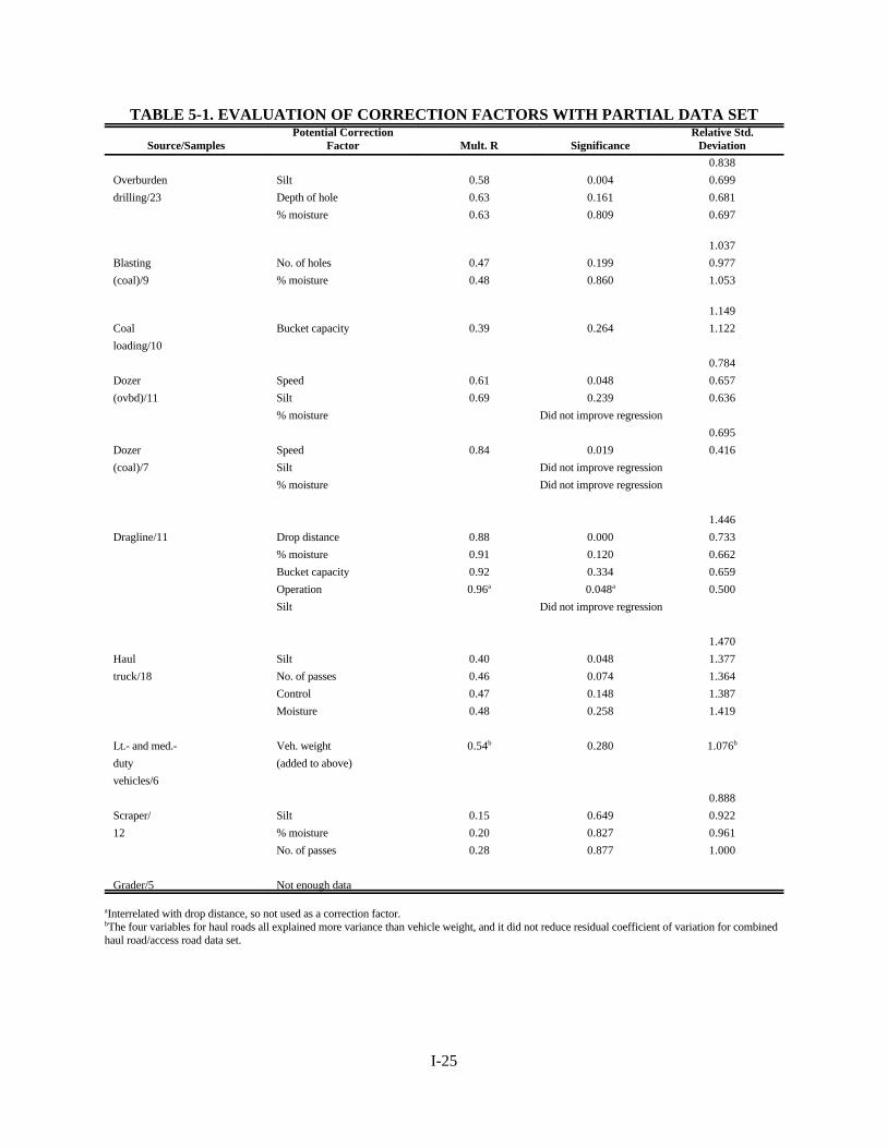
I-25
TABLE 5-1. EVALUATION OF CORRECTION FACTORS WITH PARTIAL DATA SET
Source/SamplesPotential Correction
Factor Mult. R SignificanceRelative Std.
Deviation
0.838
Overburden Silt 0.58 0.004 0.699
drilling/23 Depth of hole 0.63 0.161 0.681
% moisture 0.63 0.809 0.697
1.037
Blasting No. of holes 0.47 0.199 0.977
(coal)/9 % moisture 0.48 0.860 1.053
1.149
Coal Bucket capacity 0.39 0.264 1.122
loading/10
0.784
Dozer Speed 0.61 0.048 0.657
(ovbd)/11 Silt 0.69 0.239 0.636
% moisture Did not improve regression
0.695
Dozer Speed 0.84 0.019 0.416
(coal)/7 Silt Did not improve regression
% moisture Did not improve regression
1.446
Dragline/11 Drop distance 0.88 0.000 0.733
% moisture 0.91 0.120 0.662
Bucket capacity 0.92 0.334 0.659
Operation 0.96a 0.048a 0.500
Silt Did not improve regression
1.470
Haul Silt 0.40 0.048 1.377
truck/18 No. of passes 0.46 0.074 1.364
Control 0.47 0.148 1.387
Moisture 0.48 0.258 1.419
Lt.- and med.- Veh. weight 0.54b 0.280 1.076b
duty (added to above)
vehicles/6
0.888
Scraper/ Silt 0.15 0.649 0.922
12 % moisture 0.20 0.827 0.961
No. of passes 0.28 0.877 1.000
Grader/5 Not enough data
aInterrelated with drop distance, so not used as a correction factor.bThe four variables for haul roads all explained more variance than vehicle weight, and it did not reduce residual coefficient of variation for combinedhaul road/access road data set.
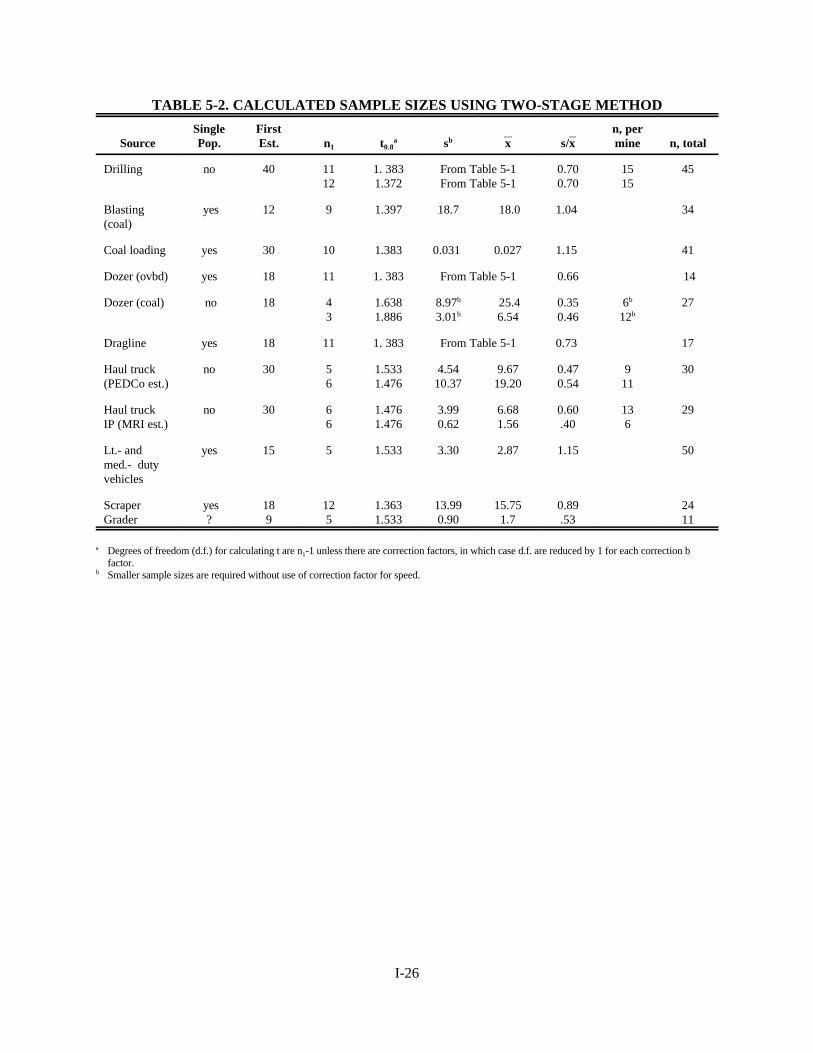
I-26
TABLE 5-2. CALCULATED SAMPLE SIZES USING TWO-STAGE METHOD
SourceSinglePop.
FirstEst. n1 t0.8
a sb x s/xn, permine n, total
Drilling no 40 1112
1. 3831.372
From Table 5-1From Table 5-1
0.700.70
1515
45
Blasting(coal)
yes 12 9 1.397 18.7 18.0 1.04 34
Coal loading yes 30 10 1.383 0.031 0.027 1.15 41
Dozer (ovbd) yes 18 11 1. 383 From Table 5-1 0.66 14
Dozer (coal) no 18 43
1.6381.886
8.97b
3.01b 25.46.54
0.350.46
6b
12b27
Dragline yes 18 11 1. 383 From Table 5-1 0.73 17
Haul truck (PEDCo est.)
no 30 56
1.5331.476
4.5410.37
9.6719.20
0.470.54
911
30
Haul truck IP (MRI est.)
no 30 66
1.4761.476
3.990.62
6.681.56
0.60.40
136
29
Lt.- andmed.- dutyvehicles
yes 15 5 1.533 3.30 2.87 1.15 50
ScraperGrader
yes?
189
125
1.3631.533
13.990.90
15.751.7
0.89.53
2411
a Degrees of freedom (d.f.) for calculating t are n1-1 unless there are correction factors, in which case d.f. are reduced by 1 for each correction bfactor.
b Smaller sample sizes are required without use of correction factor for speed.

I-27
TABLE 5-3. SAMPLE SIZES PROPOSED AND OBTAINED
Source
SamplesProposed inStudy dsn
SamplesRequired by
2-StageMethod
SamplesProposed in
Stat Plan
Rel. Errorfor Samplesin Stat Plan
SamplesActuallyCollect
Drilling 40 45 30 0.20 30
Blasting (coal) 12 34 16 0.36 16
Coal loading 30 41 24 0.32 25
Dozer (ovbd) 18 14 16 0.31 15
Dozer (coal) 18 27 10 0.31 12
Dragline 18 17 19 0.21 19
Haul truck 30 30 40 0.19 36
Lt.- and med. - dutyvehicles
15 50 12a 0.45a 12
Scrapers 18 24 24 0.24 15
Graders 9 11 8 0.27 7
aExpected to be combined with haul roads in a single emission factor.

I-28
TABLE 5-4. FF22 METHOD OF DETERMINING ATMOSPHERIC STABILITY CLASS
FF22 Stability Class
F2 >22.5E17.5 <F2 <22.512.5 <F2 <17.5
F2 <12.5
ABCD
(F2 <7.5° would be E stability, but D would be used because all sampling occurred during daytime and E isonly a nighttime stability class)
Source: Mitchell 1979.

I-29
Figure 5-1. Illustration of exposure profile extrapolation procedures (haul truck J-9).
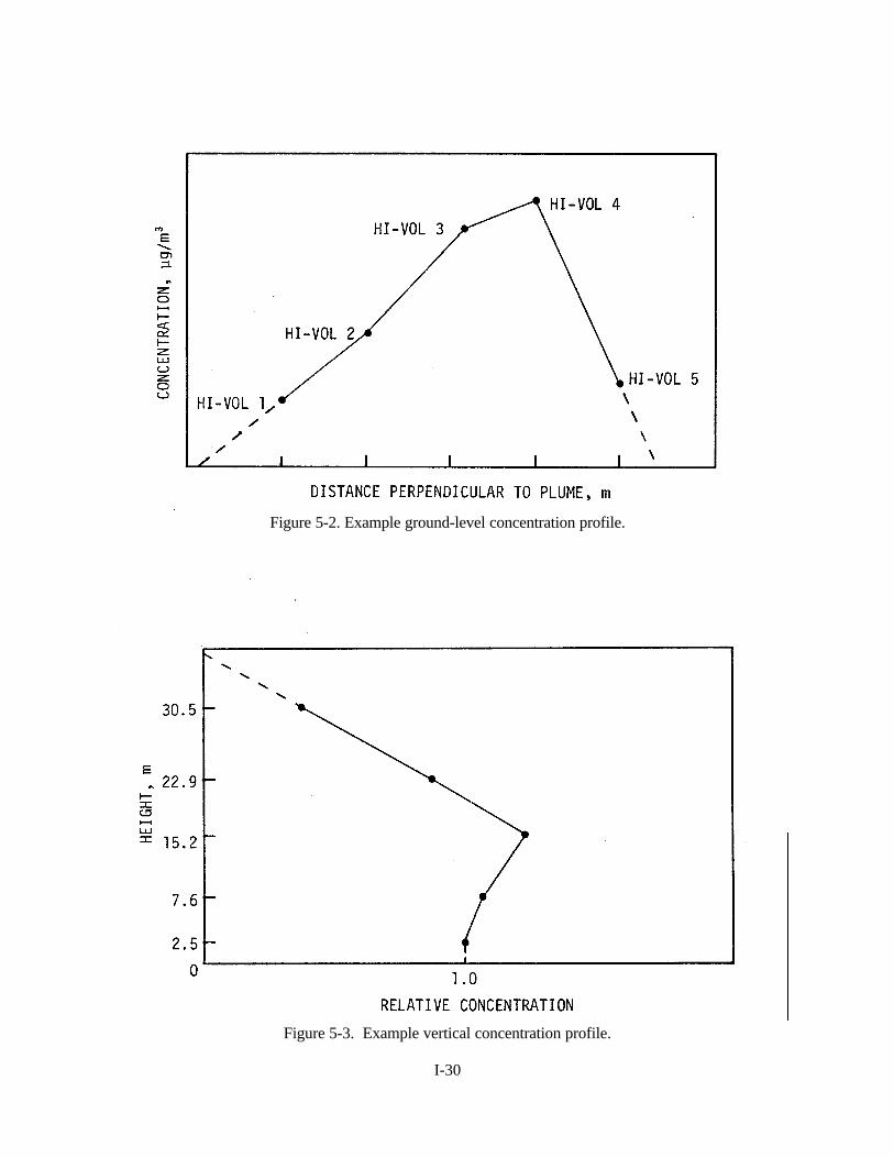
I-30
Figure 5-2. Example ground-level concentration profile.
Figure 5-3. Example vertical concentration profile.

I-31
Figure 5-4. Plot of the 50 percent cut point of the inlet versus wind speed.

I-32
SECTION 13
DEVELOPMENT OF CORRECTION FACTORS
AND EMISSION FACTOR EQUATIONS
The method for developing correction factors was based on multiple linear regression (MLR), as
described in Section 5 (Page 5-32). To summarize the method briefly, values for all variables being
considered as possible correction factors were tabulated by source with the corresponding TSP emission
rates for each test, then the data were transformed to their natural logarithms. The transformed data were
input to the MLR program, specifying the stepwise option and permitting entry of all variables that in-
creased the multiple regression coefficient (initially allowing the program to determine the order of entry of
the variables).
The MLR output of greatest interest was the significance of each variable. In nontechnical terms,
significance is the probability that the observed relationship between the independent and dependent
variables is due to chance. If the significance was less than 0.05, the variable was included as a correction
factor; if it was between 0.05 and 0.20, its inclusion was discretionary; and if above 0.20, the variable was
not included. The correction factors were multiplicative because of the ln transformation; the power for
each significant correction factor was specified in the MLR output as the coefficient (B value) for that
variable in the linear regression equation.
This MLR analysis could not be employed with data from the wind erosion sources because
sequential tests were found to be related and were grouped, thus reducing the number of independent data
points. With the large number of potential correction parameters in relation to data points, regression
analysis was not feasible.
MULTIPLE LINEAR REGRESSION ANALYSIS
The stepwise multiple linear regression program that is the nucleus of the correction factor
development procedure is explained in moderate detail in Appendix A. Further information on it can be
found in the following three references: Statistical Methods, Fourth Edition (Snedecor 1946); Applied
Regression Analysis (Draper and Smith 1965); and SPSS, Second Edition (Nie 1975).
The independent variables that were evaluated as possible correction factors are listed in
Table 13-1. An assessment was made during the MLR analysis to determine the portion of the total
variation in the emission factors explained by the correction factors (multiple regression coefficient
squared) and whether additional variables should have been considered. The data for each of these
variables were presented in tables throughout Sections 7 through 11 (Volume I), and have not been
repeated here.
I-33
The data were all transformed to their natural logarithms prior to running MLR. The presumption
that the ln transformation would provide better final emission factor equations was based on three
considerations: the data sets all had high relative standard deviations indicating that the distributions of the
emission factor were skewed to the right (i.e., a long upper tail); the homogeneity of variances (a condition
for any least squares analysis) was increased; and multiplicative correction factors were preferable to
additive ones.
More than one MLR run was usually required to obtain the final MLR equation, with its
associated significance and regression coefficients (B values). Second and third runs were needed to
eliminate a data point shown to be an outlier, to remove a variable highly correlated with another, to
remove a variable with significance of 0.05 to 0.20 that entered the stepwise regression ahead of another
variable still being evaluated, or to eliminate a dummy variable (such as a source subcategory or control/no
control) after its significance had been determined. The sequence of MLR runs with the TSP data for each
source is documented by presenting in Table 13-2 the results of the first run for each source (with all the
variables included), a description in Table 13-3 of all changes made to get to the final run, and in Table 13-
4 the results of the final run.
The multiple regression (correlation) coefficient, R. is a measure of how well the variables in the
equation explain variations in emission rate. (Actually, R2 is the portion of the total variation explained by
the use of the specified variables). Significance, the second reported statistic, estimates the chance that the
observed correlation for a particular variable is due to random variation. Finally, the residual relative
standard deviation measures the amount of variability left in the transformed data set after adjustment as
indicated by the regression equation. In the transformed data set, the mean logarithmic values can be quite
small. Consequently, the relative standard deviations are larger than normally encountered in regression
analysis.
Several independent variables were fairly significant (less than 0.20) when they entered the
regression equations, but were not included as correction factors in the final emission factors. The reasons
for omitting these potential correction factors are explained below, by source:
Drills/Silt -This variable was highly significant but was inversely rather than directly related to emission
rate. Therefore, the last potential correction factor for this source is eliminated; the reported emission
factor is simply the geometric mean of the observed values.
Blasts/No. of holes -This variable was highly correlated with another independent variable, area blasted,
which entered the regression equation before number of holes.

I-34
Coal loading/Bucket size -Bucket size was related to emission rate by a power of -12.3 in the regression
equation, primarily because of the very narrow range of bucket sizes tested--14 to 17 yd3 . Also, bucket
size only had a correlation of 0.05 with emission rate.
Dozer, all/Dozer speed - Although equipment speed was significant in the combined data set, it was not
significant in either of the subsets (coal dozers or overburden dozers).
Dragline/Silt - In the first run, silt was not a significant variable. However, when an outlier was removed, it
became highly significant but was inversely rather than directly related to emission rate.
Scrapers/Vehicle speed - This parameter was significant at the 0.111 level, in the discretionary range. It
was omitted because of its high correlation with silt which entered the equation earlier.
Light- and medium-duty vehicles/Weight - This was omitted to preserve the simplicity of the resulting
equation in light of the high correlation between emission factor and moisture, the first parameter
entered.
Haul trucks/Vehicle speed - Inverse relationship with emission rate was inconsistent with all previous
studies.
Haul trucks/Weight - This parameter was omitted because its coefficient was negative, which is difficult to
justify from the physics of the problem.
These relationships conflicted with previous experience in fugitive dust testing. While the actual
relationship may be similar to that indicated by the MLR equation, some confirmation in the form of
additional data was thought to be needed before including these dubious parameters as correction factors.
The transformations, initial MLR runs, adjustments, and additional MLR runs were done by the
same procedures with the IP emission data as with the TSP data, using the same values of the independent
variables. The results are summarized in an analogous series of three tables—Tables 13-5, 13-6, and 13-7.
As indicated in Table 13-6, very few changes were required from the initial runs of the IP data, with the
benefit of the prior TSP runs. For every source, the same independent variables were highly significant for
IP as for TSP.
EMISSION FACTOR PREDICTION EQUATIONS
The prediction equations obtained from the MLR analyses are summarized in Table 13-8. These
equations were taken directly from the MLR runs described in Tables 13-4 and 13-7, with the coefficients
in the Table 13-8 equations being the exponentials of the MLR equation constant terms and the exponents
for each term being the B values. These equations give estimates of the median value of the emission
factors for given value(s) of the correction factor(s). (The coefficients and exponents are from the
intermediate MLR step that includes only the significant variables that appear in the final equation.) All but

I-35
four of the independent variables in the equations in Table 13-8 are significant at the 0.05 level or better.
The four variables in the discretionary range (0.05 to 0.20) that were included are: L in haul truck TSP
equation, % = 0.146; A in the coal blasting IP equation,% = 0.051; M in the overburden IP equation, % =
0.071; and S in the grader IP equation, % = 0.078. The geometric mean values and ranges of the correction
factors are summarized in Table 13-9.
CONFIDENCE AND PREDICTION INTERVALS
A computational procedure for obtaining confidence and prediction intervals for emission factors is
described in Appendix B at the end of this volume of the report. An example of this computation is given
here for coal loading emission data versus the moisture content correction factor.
Figure 13-1 summarizes the results of this example and also includes the observed emission
factors. The line in the center of the graph is the predicted median emission rate estimated by the geometric
mean. The inside set of curves give the confidence interval for the “true median” as a function of moisture
content (M), and the outside set of curves give the prediction interval for an individual emission factor. The
intervals vary in length as a function of M. The widths of the intervals are measures of the precision of the
estimated factors. These precisions are comparable to those of existing emission factors as illustrated in
Section 14.
To summarize the information contained in these curves for confidence intervals, the following
information is presented:
1. Prediction equation for the media emission factor from Table 13-8: TSP, lb/ton = 1.16/M1.2.
2. Geometric mean and range (maximum and minimum values) of moisture content correction
factor from Table 13-9: GM = 17.8 percent, 6.6 to 38 percent.
3. Estimated median emission factor at the geometric mean (GM) of the correction factor from
Table 13-10: 0.034 lb/ton.
4. Ninety-five percent confidence intervals for the median emission factor (the median value for a
large number of tests over one year) at the GM of each correction factor from Table 13-10: 0.023 lb/ton to
0.049 lb/ton.
5. Ninety-five percent prediction intervals for an individual emission factor (approximately one
hour) at the GM of the correction factor from Table 13-10: 0.005 lb/ton to 0.215 lb/ton.
The confidence and prediction interval data are given only for one value of the correction factor(s)
in order to simplify the presentation. The widths of the intervals at the GM are indicative of the widths at
other values provided one uses a percentage of the median value in deriving the confidence and prediction
limits. For example, for the coal loading data the lower confidence limits are approximately 50 to 70
percent of the median value, the upper limits are 140 to 170 percent of the median value; the lower

I-36
prediction limits are 15 percent of the median value and the upper limits are 630 percent (or 6.3 times) of
the median value. The coal loading data are slightly more variable than data for other sources and hence the
limits are proportionately wider than for the other sources.
Fine particulate (FP) emission factors were not developed by the same series of steps as were the
TSP and IP factors, because of the larger variances expected in these data sets and the many tests with
negligible readings. However, the relative standard deviations calculated from data in Table 12-2 indicate
variability approximately the same as for TSP and IP data. The geometric mean ratios of FP to TSP
presented in Table 13-8 are proposed for use with the TSP emission factor equations to derive FP emission
factors. The FP emission factor is obtained by multiplying the median FP/TSP ratio times the calculated
TSP emission factor for each source.
EMISSION FACTORS FOR WIND EROSION SOURCES
In nearly all of the tests of wind erosion emissions from the surfaces of coal piles and exposed
ground areas, the SP and IP emission rates were found to decay sharply with time. An exception was the
sandy topsoil tested at Mine 3; in that case, an increase in emission rate was observed, probably because of
the entrainment effect of infiltration air as the loose soil surface receded below the sides of the wind tunnel.
The concept of erosion potential was introduced in Section 5 to treat the case of an exponentially
decreasing quantity of erodible material on the test surface. The erosion potential is the total quantity of
particles, in any specified particle size range, present on the surface (per unit area) that can be removed by
erosion at a particular wind speed.
The calculation of erosion potential necessitated grouping of sequential tests on the same surface.
In effect, this reduced the number of independent data points for coal and overburden emissions from 32 to
16. As a result, the decision was made not to subject these data to regression analysis because of the large
number of potentially significant correction parameters in relation to the number of emission measurements
for any given surface type and condition.
Table 13-11 lists the calculated values of erosion potential classified by erodible surface type and
by wind speed at the tunnel centerline. For the most part, the test wind speeds fit into 3-mph increments;
values of erosion potential for the few runs performed at other wind speeds are listed under the nearest
wind speed category. Whenever erosion potential is given as a range, the extremes represent two data
points obtained at nominally the same conditions.

I-37
lnMo & L1
Mo
lnMo & L2
Mo
't1
t2
(Eq. 22)
l &L2
Mo
' l &L1
Mo
t2
t1
(Eq. 22a)
Erosion potential was calculated using Equation 22 (Chapter 5), which is repeated here:
where Mo = erosion potential, i.e., quantity of erodible material present on the surface before the
onset of erosion, g/m2
t = cumulative erosion time, s
L1 = measured loss during time period 0 to t1, g/m2
L2 = measured loss during time period 0 to t2, g/m2
Alternatively, Equation 22 can be rewritten as follows:
An iterative calculation procedure was required to calculate erosion potential from Equation 22 or
22a. Further, two cumulative loss values and erosion times obtained from back-to-back testing of the same
surface were required. Each loss value was calculated as the product of the emission rate and the erosion
time.
For example, Runs P-27 and P-28 took place on a coal pile furrow at a tunnel centerline wind
speed of 36 mph. The incremental losses were calculated as follows:
P-27: 0.0386 g/m2-s x 120 s = 4.63 g/m2
P-28: 0.00578 g/m2-s x 480 s = 2.77 g/m2
Thus the values substituted into Equation 22 for this test series were:
L1 = 4.63 g/m2
t1 = 120 s
L2 = 4.63 + 2.77 = 7.40 g/m2
t2 = 120 + 480 = 600 s
A value of Mo = 10 was selected and substituted into the right-hand side of Equation 22a and the
left-hand side was solved for Mo. The resulting value of 7.75 was then substituted back into the right-hand
side to obtain a new solution--7.48. Additional substitutions were made and the iteration procedure
converged quickly to 7.46 for erosion potential (Mo), indicating that only a small additional loss (0.06 g/m2)
I-38
would have occurred if the tunnel had been operated beyond the 600-s time period at the same wind speed.
The corresponding nonmetric value for the erosion potential is 67 lb/acre, which rounds to 70 lb/acre.
Data from unpaired runs (J-26, J-27, K-39, P-20, and K-37) were used to derive estimated values
of erosion potential. Except for J-26, the erosion times were long enough so that the measured losses
approximated the corresponding erosion potentials.
Note that whenever a surface was tested at sequentially increasing wind speeds, the measured
losses from the lower speeds were added to the losses at the next higher speeds and so on. This reflects the
hypothesis that, if the lower speeds had not been tested beforehand, correspondingly greater losses would
have occurred at the higher speeds.
The emissions from the coal pile at Mine 3 appear to be significantly lower than the coal pile
emissions measured at Mines 1 and 2. The coal pile at Mine 3, which had been inactive for a period of
days, was noticeably crusted; but attempts were made to test areas where relatively fresh vehicle tracks
were present. It is not known what percentage of the erosion potential of these test areas may have been lost
because of brief periods of high winds which typically occurred with the evening wind shift. The coal pile
furrow tested at Mine 3 had a much greater portion of large chunks of coal (exceeding 1 inch in size) on the
surface, in comparison with the scraper and truck tracks.
The uncrusted overburden and scoria surfaces tested at Mine 2 exhibited emission rates that were
much lower than the coal surfaces tested, except for the coal pile furrow. This reflects the larger portion of
nonerodible coarse aggregates present on these non-coal surfaces.
The wind speeds that were used in the testing (Table 13-11), which exceeded the threshold for the
onset of visually observable emissions, corresponded to the upper extremes of the frequency distributions of
hourly mean wind speeds observed (at a height of 5-10 m) for most areas of the country. For flat surfaces,
the wind speed at the centerline of the wind tunnel, 15 cm above the surface, is about half the value of the
wind speed at the 10 m reference height. However, for elevated pile surfaces, particularly on the windward
faces, the ratio (u15+/uref) may approach and even exceed unity. It should be noted that smart but
measurable erosion may have occurred at the threshold velocity.
In estimating the magnitude of wind generated emissions, wind gusts must also be taken into
account. For the surfaces tested, typically about three-fourths of the erosion potential was emitted within 5
min of cumulative erosion time. Therefore, although the mean wind speeds at surface coal mines will
usually not be high enough to produce continuous wind erosion, gusts may quickly deplete the erosion
potential over a period of a few hours. Because erosion potential increases rapidly with increasing wind
speed, estimated emissions should be related to the gusts of highest magnitude.

I-39
Emission Factor ' f @ P(u%
15) (Eq. 29)
The routinely measured meteorological variable which best reflects the magnitude of wind gusts is
the fastest mile. This quantity represents the wind speed corresponding to the whole mile of wind movement
which has passed by the 1-mile contact anemometer in the least amount of time. Daily measurements of the
fastest mile are presented in the monthly Local Climatological Data (LCD) summaries. The duration of the
fastest mile, typically about 2 min (for a fastest mile of 30 mph), matches well with the half life of the
erosion process, which ranges between 1 and 4 min.
Emissions generated by wind erosion are also dependent on the frequency of disturbance of the
erodible surface because each time that a surface is disturbed, its erosion potential is restored. A
disturbance is defined as an action which results in the exposure of fresh surface material. On a storage
pile, this would occur whenever aggregate material is either added to or removed from the old surface. A
disturbance of an exposed ground area may also result from the turning of surface material to a depth
exceeding the size of the largest pieces of material present.
Although vehicular traffic alters the surface by pulverizing surface material, this effect probably
does not restore the full erosion potential, except for surfaces that crust before substantial wind erosion
occurs. In that case, breaking of the crust over the area of the tire/surface contact once again exposes the
erodible material beneath.
The emission factor for wind generated emissions of a specified particle size range may be
expressed in units of lb/acre month as follows:
where f = frequency of disturbance, per month
= erosion potential corresponding to the observed (or probable) fastest mile of wind for theP(u%
15)
period between disturbances, after correcting the fastest mile to a height of 15 cm (as
described below), lb/acre.
is taken directly from Table 13-ll for the type of surface being considered. Interpolation or limitedP(u%
15)
extrapolation of erosion potential data may be required.
When applying Equation 29 to an erodible surface, a modified form of Equation 18 (Page 5-23) is
used to correct the fastest mile of wind from the reference anemometer height at the reporting weather
station to a height of 15 cm. The correction equation is as follows:
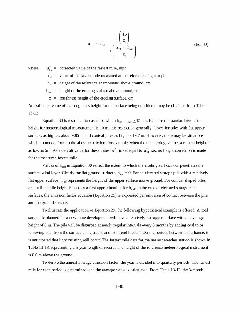
I-40
u%
15 ' u%
ref
ln 15zo
lnhref & hsurf
zo
(Eq. 30)
where = corrected value of the fastest mile, mphu%
15
= value of the fastest mile measured at the reference height, mphu%
ref
href = height of the reference anemometer above ground, cm
hsurf = height of the eroding surface above ground, cm
zo = roughness height of the eroding surface, cm
An estimated value of the roughness height for the surface being considered may be obtained from Table
13-12.
Equation 30 is restricted to cases for which href - hsurf > 15 cm. Because the standard reference
height for meteorological measurement is 10 m, this restriction generally allows for piles with flat upper
surfaces as high as about 9.85 m and conical piles as high as 19.7 m. However, there may be situations
which do not conform to the above restriction; for example, when the meteorological measurement height is
as low as 5m. As a default value for these cases, is set equal to i.e., no height correction is madeu%
15 u%
ref
for the measured fastest mile.
Values of hsurf in Equation 30 reflect the extent to which the eroding surf contour penetrates the
surface wind layer. Clearly for flat ground surfaces, hsurf = 0. For an elevated storage pile with a relatively
flat upper surface, hsurf represents the height of the upper surface above ground. For conical shaped piles,
one-half the pile height is used as a first approximation for hsurf. In the case of elevated storage pile
surfaces, the emission factor equation (Equation 29) is expressed per unit area of contact between the pile
and the ground surface.
To illustrate the application of Equation 29, the following hypothetical example is offered. A coal
surge pile planned for a new mine development will have a relatively flat upper surface with an average
height of 6 m. The pile will be disturbed at nearly regular intervals every 3 months by adding coal to or
removing coal from the surface using trucks and front-end loaders. During periods between disturbance, it
is anticipated that light crusting will occur. The fastest mile data for the nearest weather station is shown in
Table 13-13, representing a 5-year length of record. The height of the reference meteorological instrument
is 8.0 m above the ground.
To derive the annual average emission factor, the year is divided into quarterly periods. The fastest
mile for each period is determined, and the average value is calculated. From Table 13-13, the 3-month

I-41
u%
15 ' 43ln 15
0.06
ln 800&6000.06
' 29 mph
SP emission factor '0.33mo
x 140 lbacre
' 46 lbacre&mo
fastest mile values of 47, 38, 45, and 41 mph yield an average of 43 mph. Next, Equation 30 is used to
correct the average fastest mile from the reference height of 8 m to 15 cm above the 6-m height of the upper
pile surface. A value of 0.06 cm is used as the roughness height for a lightly crusted coal pile surface, as
taken from Table 13-12. Substitution of these data into Equation 30 yields:
From Table 13-11, the SP erosion potential for 29 mph on a lightly crusted coal pile is 140 lb/acre.
Substitution into Equation 29 yields:
Using the appropriate IP/SP ratio from Table 13-12, the corresponding IP emission factor is 46 x 0.55 =
25 lb/acre-mo.
One notable limitation in the use of Equation 29 is its application to active storage piles. Because
the fastest mile is recorded only once per day, use of the daily fastest mile to represent a surface disturbed
more than once per day will result in an over-estimate of emissions.
The approach outlined above for calculation of emission factors appears to be fundamentally
sound, but data limitations produce a large amount of uncertainty in the calculated factors. Even though the
erosion potential values are judged to be accurate to within a factor of two or better for the surfaces tested,
it is not known how well these surfaces represent the range of erodible surface conditions found at Western
surface coal mines. Additional uncertainty results from the use of Equation 30 to correct the fastest mile
values to a height of 15 cm above the erodible surface. Taking all the sources of uncertainty into account, it
is thought that the wind erosion emission factors derived for surfaces similar to those tested are accurate to
within a factor of about three.
The levels of uncertainty in SP and IP emission factors derived by the technique outlined in this
section could be reduced substantially by gathering more data to better define:
1. Relationship of erosion potential to wind speed.
2. Relationship between approach wind speed and the distribution of surface wind speed around
basic pile shapes of varying size.
3. Relationship of erosion potential to surface texture.
4. Effect of crusting.

I-42
Previous research on wind erosion of natural surfaces could provide some insight into the nature of
these effects. Soil loss resulting from wind erosion of agricultural land has been the subject of field and
laboratory investigation for a number of years. This research has focused on the movement of total soil
mass, primarily sand-sized aggregates, as a function of wind and soil conditions (Bagnold 1941; Chepil and
Woodruff 1963). Only relatively recently, however, have field measurements been performed in an effort to
quantify fine particle emissions produced during wind erosion of farm fields (Gillette and Blifford 1972;
Gillette 1978).
Until further research is accomplished, it is recommended that wind erosion factors be used with
full consideration of their uncertainty and preliminary nature. It is recommended that their use be restricted
to estimates of emissions relative to other mine sources and that they not be used for estimating the ambient
air impact of wind erosion at surface coal mines.
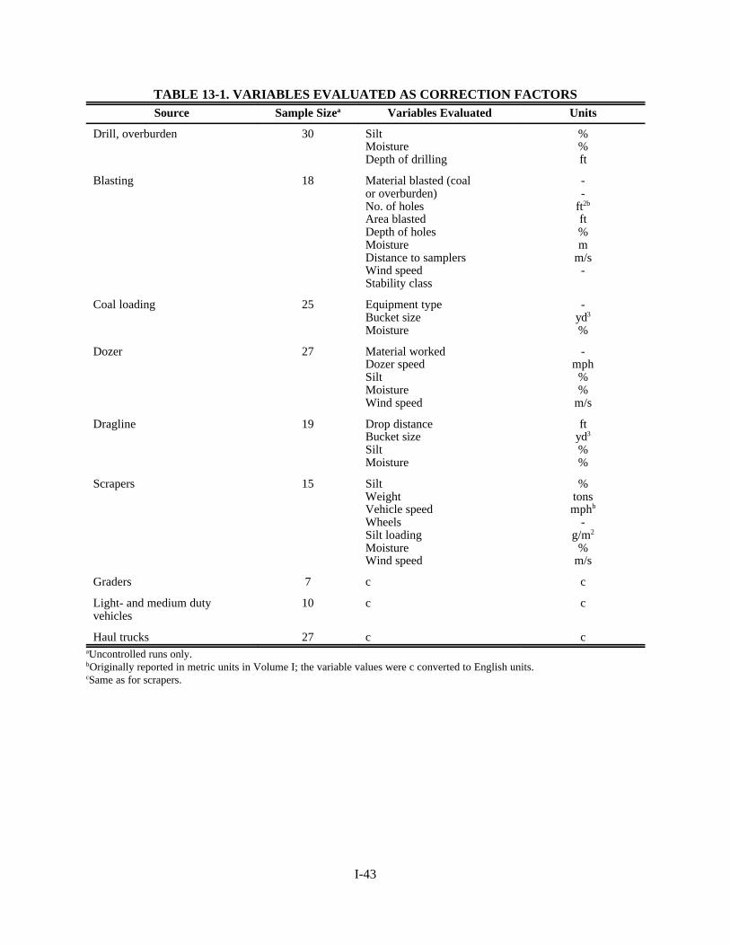
I-43
TABLE 13-1. VARIABLES EVALUATED AS CORRECTION FACTORSSource Sample Sizea Variables Evaluated Units
Drill, overburden 30 SiltMoistureDepth of drilling
%%ft
Blasting 18 Material blasted (coalor overburden)No. of holesArea blastedDepth of holesMoistureDistance to samplersWind speedStability class
--
ft2b
ft%m
m/s-
Coal loading 25 Equipment typeBucket sizeMoisture
-yd3
%
Dozer 27 Material workedDozer speedSiltMoistureWind speed
-mph
%%
m/s
Dragline 19 Drop distanceBucket sizeSiltMoisture
ftyd3
%%
Scrapers 15 SiltWeightVehicle speedWheelsSilt loadingMoistureWind speed
%tonsmphb
-g/m2
%m/s
Graders 7 c c
Light- and medium dutyvehicles
10 c c
Haul trucks 27 c caUncontrolled runs only.bOriginally reported in metric units in Volume I; the variable values were c converted to English units.cSame as for scrapers.
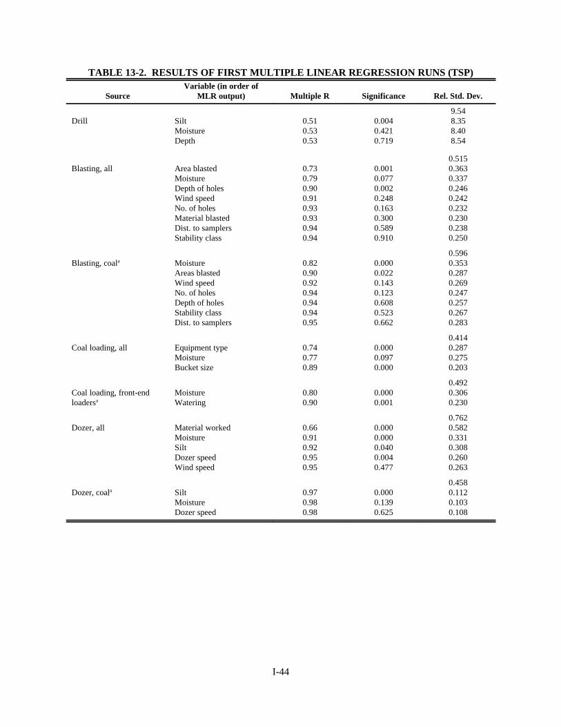
I-44
TABLE 13-2. RESULTS OF FIRST MULTIPLE LINEAR REGRESSION RUNS (TSP)
SourceVariable (in order of
MLR output) Multiple R Significance Rel. Std. Dev.
Drill SiltMoistureDepth
0.510.530.53
0.0040.4210.719
9.548.358.408.54
Blasting, all Area blastedMoistureDepth of holesWind speedNo. of holesMaterial blastedDist. to samplersStability class
0.730.790.900.910.930.930.940.94
0.0010.0770.0020.2480.1630.3000.5890.910
0.5150.3630.3370.2460.2420.2320.2300.2380.250
Blasting, coala MoistureAreas blastedWind speedNo. of holesDepth of holesStability classDist. to samplers
0.820.900.920.940.940.940.95
0.0000.0220.1430.1230.6080.5230.662
0.5960.3530.2870.2690.2470.2570.2670.283
Coal loading, all Equipment typeMoistureBucket size
0.740.770.89
0.0000.0970.000
0.4140.2870.2750.203
Coal loading, front-endloadersa
MoistureWatering
0.800.90
0.0000.001
0.4920.3060.230
Dozer, all Material workedMoistureSiltDozer speedWind speed
0.660.910.920.950.95
0.0000.0000.0400.0040.477
0.7620.5820.3310.3080.2600.263
Dozer, coala SiltMoistureDozer speed
0.970.980.98
0.0000.1390.625
0.4580.1120.1030.108

I-45
TABLE 13-2 (continued)
SourceVariable (in order of
MLR output) Multiple R Significance Rel. Std. Dev.
Dozer, overburdena MoistureSiltDozer speed
0.780.870.91
0.0010.0290.072
0.8670.5660.4710.417
Dragline Drop distanceMoistureSiltBucket size
0.740.850.860.87
0.0000.0040.3650.147
0.4160.2880.2290.2300.236
Scrapers (all uncontrolled) WeightMoistureWheelsSiltVehicle speedSilt loadingWind speed
0.680.800.850.940.960.970.97
0.0220.0760.2320.0280.1870.3180.794
0.5260.4070.3500.3360.2350.2120.2060.235
Graders (all uncontrolled)b Silt loadingVehicle speedWheels
0.400.630.96
0.5000.4710.226
16.93317.90918.6149.144
Light- and medium-dutyvehicles (all uncontrolled)c
MoistureWeightWheelsSiltSilt loadingWind speed
0.970.990.990.991.001.00
0.0000.0050.3490.6810.1330.202
6.5621.7411.0191.0171.0930.8900.749
Haul trucks (includesuw. -dw. tests, all uncontrolled)
Vehicle speedWind speedMoistureSilt loadingWheelsWeightSilt
0.510.720.890.910.910.920.92
0.0110.0030.0000.0390.7010.3180.886
0.7880.6930.5730.3900.3570.3650.3640.375
a This source was evaluated initially as a subset of the entire data set and was not carried through the subsequent dataanalyses.
b Weight, moisture, silt, and wind speed were rejected in the first MLR because of an insufficient tolerance level.c Vehicle speed was rejected because of an insufficient tolerance level.
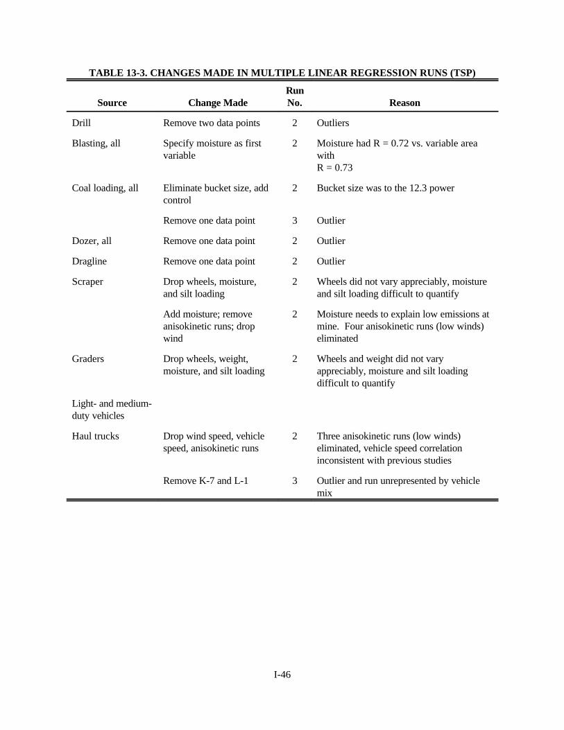
I-46
TABLE 13-3. CHANGES MADE IN MULTIPLE LINEAR REGRESSION RUNS (TSP)
Source Change MadeRunNo. Reason
Drill Remove two data points 2 Outliers
Blasting, all Specify moisture as firstvariable
2 Moisture had R = 0.72 vs. variable areawithR = 0.73
Coal loading, all Eliminate bucket size, addcontrol
2 Bucket size was to the 12.3 power
Remove one data point 3 Outlier
Dozer, all Remove one data point 2 Outlier
Dragline Remove one data point 2 Outlier
Scraper Drop wheels, moisture,and silt loading
2 Wheels did not vary appreciably, moistureand silt loading difficult to quantify
Add moisture; removeanisokinetic runs; dropwind
2 Moisture needs to explain low emissions atmine. Four anisokinetic runs (low winds)eliminated
Graders Drop wheels, weight,moisture, and silt loading
2 Wheels and weight did not varyappreciably, moisture and silt loadingdifficult to quantify
Light- and medium-duty vehicles
Haul trucks Drop wind speed, vehiclespeed, anisokinetic runs
2 Three anisokinetic runs (low winds)eliminated, vehicle speed correlationinconsistent with previous studies
Remove K-7 and L-1 3 Outlier and run unrepresented by vehiclemix

I-47
TABLE 13-4. RESULTS OF FINAL MULTIPLE LINEAR REGRESSION RUNS (TSP)
Source Variable Multiple R Significance Rel. Std. Dev.
5.30Drill Silt 0.59 0.001 4.36
0.515Blasting, all Moisture 0.72 0.001 0.367
Depth 0.84 0.009 0.300Area 0.90 0.012 0.246
0.341Coal loading, all Moisture 0.67 0.000 0.258
Control 0.77 0.012 0.2270.774
Dozer, all Material worked 0.67 0.000 0.587Moisture 0.93 0.000 0.298Silt 0.95 0.005 0.253Dozer speed 0.97 0.003 0.210
0.389Dragline Drop distance 0.80 0.000 0.241
Moisture 0.91 0.001 0.172Silt 0.93 0.043 0.153
0.647Scrapers Silt 0.70 0.036 0.494
Weight 0.93 0.006 0.271Vehicle speed 0.96 0. 111 0. 225Moisture 0.96 0.634 0.243
2.013Graders Vehicle speed 0.83 0.022 1.237
Wind speed 0.87 0.333 1.212Silt 0.90 0.451 1.252
6.562Light- and Moisture 0.97 0.000 1.741medium-duty Weight 0.99 0.005 1.019vehicles Wheels 0.99 0.349 1.017
Silt 0.99 0.681 1.093Silt loading 1.00 0.133 0.890Wind speed 1.00 0.202 0.749
0.540Haul trucks Wheels 0.66 0.002 0.416
Silt loading. 0.72 0.146 0.400Weight 0.80 0.036 0.355Silt 0.82 0.324 0.355Moisture 0.82 0.458 0.360

I-48
TABLE 13-5. RESULTS OF FIRST MULTIPLE LINEAR REGRESSION RUNS (IP)
SourceVariable (in order
of MLR output) Multiple R SignificanceRel. Std.
Dev.
Drill N/A 9.54
0.753
Blasting, all Moisture 0.81 0.015 0.367
Depth of holes 0.88 0.040 0.330
Area blasted 0.92 0.000 0.451
Wind speed 0.93 0.210 0.321
No. of holes 0.94 0.225 0.312
Material blasted 0.95 0.272 0.307
Dist. to samplers 0.95 0.313 0.305
Stability class 0.95 0.841 0.323
0.933
Blasting, coala Moisture 0.86 0.000 0.490
Areas blasted 0.91 0.050 0.421
No. of holes 0.93 0.146 0.392
Wind speed 0.94 0.202 0.373
Dist. to samplers 0.96 0.248 0.360
Stability class 0.96 0.489 0.373
0.235
Coal loading, all Moisture 0.49 0.017 0.210
Control 0.66 0.017 0.185
Equipment type 0.67 0.576 0.189
1.569
Dozer, all Material worked 0.71 0.000 1.132
Moisture 0.91 0.000 0.683
Silt 0.94 0.006 0.579
Dozer speed 0.97 0.001 0.449
0.682
Dozer, coala Moisture 0.91 0.000 0.291
Silt 0.96 0.012 0.213
Dozer speed 0.96 0.420 0.216
8.262
Dozer, overburdena Silt 0.77 0.004 5.550
Moisture 0.85 0.071 4.830
Dozer speed 0.87 0.290 4.756
0.259
Dragline Moisture 0.49 0.032 0.232
Drop distance 0.69 0.015 0.197
Silt.72 0.72 0.281 0.196
Bucket size 0.73 0.582 0.200
a This source was evaluated initially as a subset of the entire data set and was not carried through the subsequent data analyses.

I-49
TABLE 13-5 (continued)
SourceVariable (in order
of MLR output) Multiple R SignificanceRel. Std.
Dev.
0.987
Scrapers (all uncontrolled) Weight 0.71 0.015 0.735
Moisture 0.81 0.094 0.647
Wheels 0.86 0.173 0.600
Silt 0.93 0.058 0.469
Vehicle speed 0.96 0.086 0.371
Silt loading 0.98 0.238 0.341
Wind speed 0.98 0.737 0.386
0.906
Graders (all uncontrolled) Silt 0.30 0.626 0.998
Wheels 0.65 0.397 0.975
Silt loading 0.87 0.442 0.883
1.977
Light- and medium-duty Silt loading 0.97 0.000 0.526
vehicles (all uncontrolled) Silt 0.98 0.043 0.410
Vehicle speed 0.99 0.010 0.243
Wind speed 1.00 0.044 0.170
1.991
Haul trucks (includes Vehicle speed 0.40 0.046 1.861
uw.-dw. tests, all Wind speed 0.64 0.006 1.600
uncontrolled) Moisture 0.84 0.000 1.153
Silt loading 0.84 0.695 1.177
Wheels 0.84 0.754 1.205
Weight 0.85 0.609 1.228
Silt 0.85 0.724 1.259
a This source was evaluated initially as a subst of the entire data set and was not carried through the subsequentdata analyses.

I-50
TABLE 13-6. CHANGES MADE IN MULTIPLE LINEAR REGRESSION RUNS (IP)
Source Change Made Run No. Reason
Blasting, all None
Coal loading, all None
Dozer, all Remove one data point 2 Outlier
Dragline None
Scrapers Drop wheels, silt loading,wind speed; removeanisokinetic runs
2 Wheels did not varyappreciably, silt loadingdifficult to quantify; fouranisokinetic runs (lowwinds) eliminated
Graders Drop wheels, weight,moisture, and silt loading
2 Wheels and weight did notvary appreciably; moistureand silt loading difficult toquantify
Light- and medium-dutyvehicles
None
Haul trucks Drop wind speed, vehiclespeed; remove anisokineticruns plus K-7 and L-1
2 Three anisokinetic runs(low winds) eliminated.Vehicle speed correlationinconsistent with previousstudies. L-1 is outlier andK-7 had unrepresentativevehicle mix

I-51
TABLE 13-7. RESULTS OF FINAL MULTIPLE LINEAR REGRESSION RUNS (IP)
Source Variable Multiple R Significance Rel. Std. Dev.
0.753Blasting, all Moisture 0.81 0.000 0.451
Depth of holes 0.88 0.015 0.376Area blasted 0.92 0.040 0.330
0.235Coal loading, all Moisture 0.49 0.017 0.210
Control 0.66 0.017 0.1851.676
Dozer, all Material worked 0.70 0.000 1.230Moisture 0.92 0.000 0.696Silt 0.95 0.006 0.583Dozer speed 0.98 0.000 0.405
0.259Dragline Moisture 0.49 0.032 0.232
Drop distance 0.69 0.015 0.1971.706
Scrapers Silt 0.67 0.046 1.346Weight 0.90 0.015 0.856Vehicle speed 0.96 0.036 0.580
3.439Graders Vehicle speed 0.70 0.078 2.680
Wind speed 0.81 0.246 2.478Silt 0.89 0.254 2.220
1.977Light- and Moisture 0.95 0.000 0.667medium-duty Weight 0.99 0.005 0.389vehicles Silt 0.99 0.084 0.321
Vehicle speed 0.99 0.217 0.298Silt loading 1.00 0.161 0.253Wind speed 1.00 0.216 0.216
1.043Haul trucks Wheels 0.65 0.003 0.816
Weight 0.68 0.272 0.809Silt loading 0.72 0.198 0.790Silt 0.73 0.617 0.810Moisture 0.74 0.473 0.823

I-52
TABLE 13-8. PREDICTION EQUATIONS FOR MEDIAN EMISSION RATES
Source
Prediction Equations FP/TSPRatios
MedianValue UnitsTSP IP
Drill 1.3 Nonea Nonea lb/hole
Blasting, all961 A 0.8
D1.8 M1.9
2550 A 0.6
D1.5 M2.30.30 lb/blast
Coal loading 1.16/M1.2 0.119/M0.9 0.019 lb/ton
Dozer, all
Coal 78.4 s1.2/M1.3 18.6 s1.5/M1.4 0.022 lb/in
Overburden 5.7 s1.2/M1.3 1.0 s1.5/M1.4 0.105 1b/h
Dragline 0.0021 d1.1/M0.3 0.0021 d0.7/M0.3 0.017 1b/yd3
Scrapers (2.7x10⁻⁵)s1.3W2.4 (6.2x10⁻⁶)s1.4W2.5 0.026 1b/VMT
Graders 0.040 S2.5 0.051 S2.0 0.031 1b/VMT
Light- and medium-duty vehicles
5.79/M4.0 3.72/M4.3 0. 040 lb/VMT
Haul trucks 0.0067 w3.4L0.2 0.0051 w3.5 0.017 1b/VMT
a Test method allowed for measurement of TSP only.
s = silt content, % W = vehicle weight, tonsA = area blasted, ft2 S = vehicle speed, mphD = depth of holes, ft w = number of wheelsM = moisture content, % L = silt loading, g/m2
d = drop distance, ft
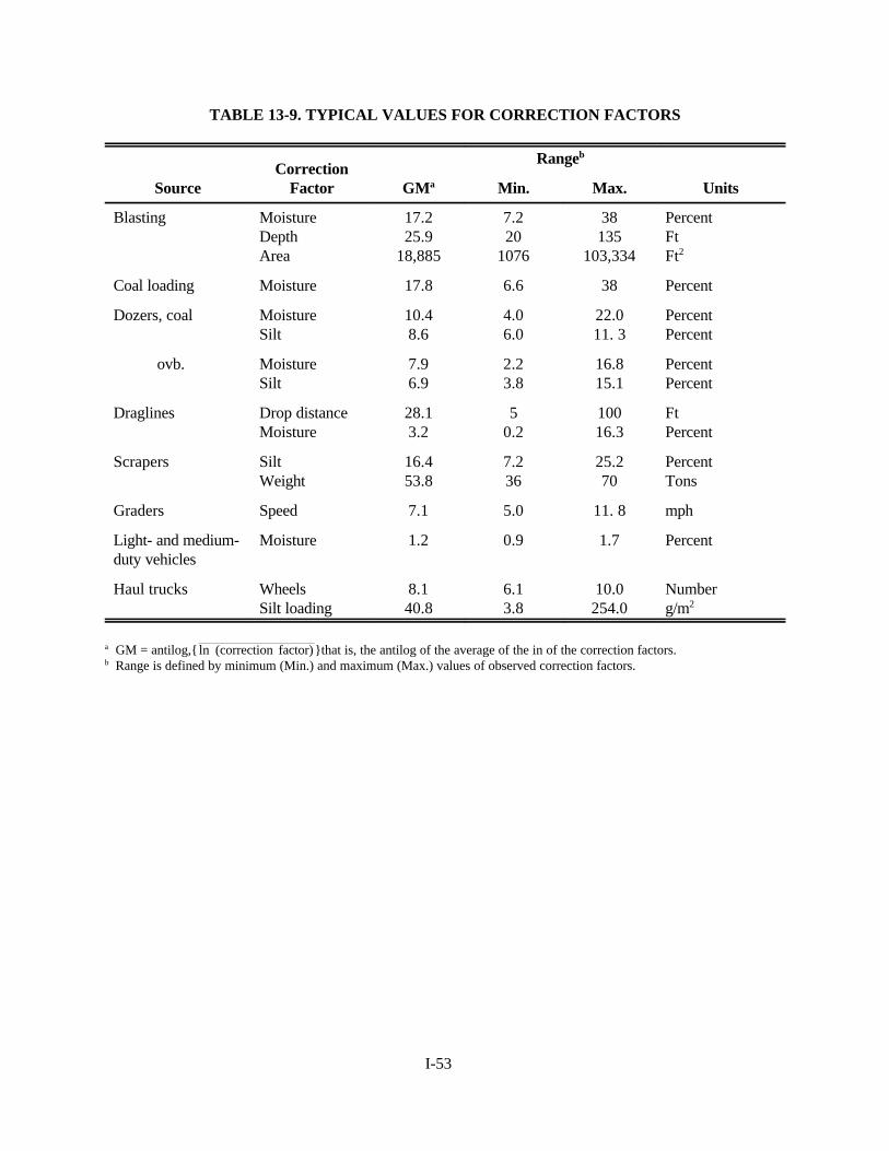
I-53
TABLE 13-9. TYPICAL VALUES FOR CORRECTION FACTORS
SourceCorrection
Factor GMa
Rangeb
UnitsMin. Max.
Blasting MoistureDepthArea
17.225.9
18,885
7.220
1076
38135
103,334
PercentFtFt2
Coal loading Moisture 17.8 6.6 38 Percent
Dozers, coal MoistureSilt
10.48.6
4.06.0
22.011. 3
PercentPercent
ovb. MoistureSilt
7.96.9
2.23.8
16.815.1
PercentPercent
Draglines Drop distanceMoisture
28.13.2
50.2
10016.3
FtPercent
Scrapers SiltWeight
16.453.8
7.236
25.270
PercentTons
Graders Speed 7.1 5.0 11. 8 mph
Light- and medium-duty vehicles
Moisture 1.2 0.9 1.7 Percent
Haul trucks WheelsSilt loading
8.140.8
6.13.8
10.0254.0
Numberg/m2
a GM = antilog,{ }that is, the antilog of the average of the in of the correction factors.ln (correction factor)b Range is defined by minimum (Min.) and maximum (Max.) values of observed correction factors.
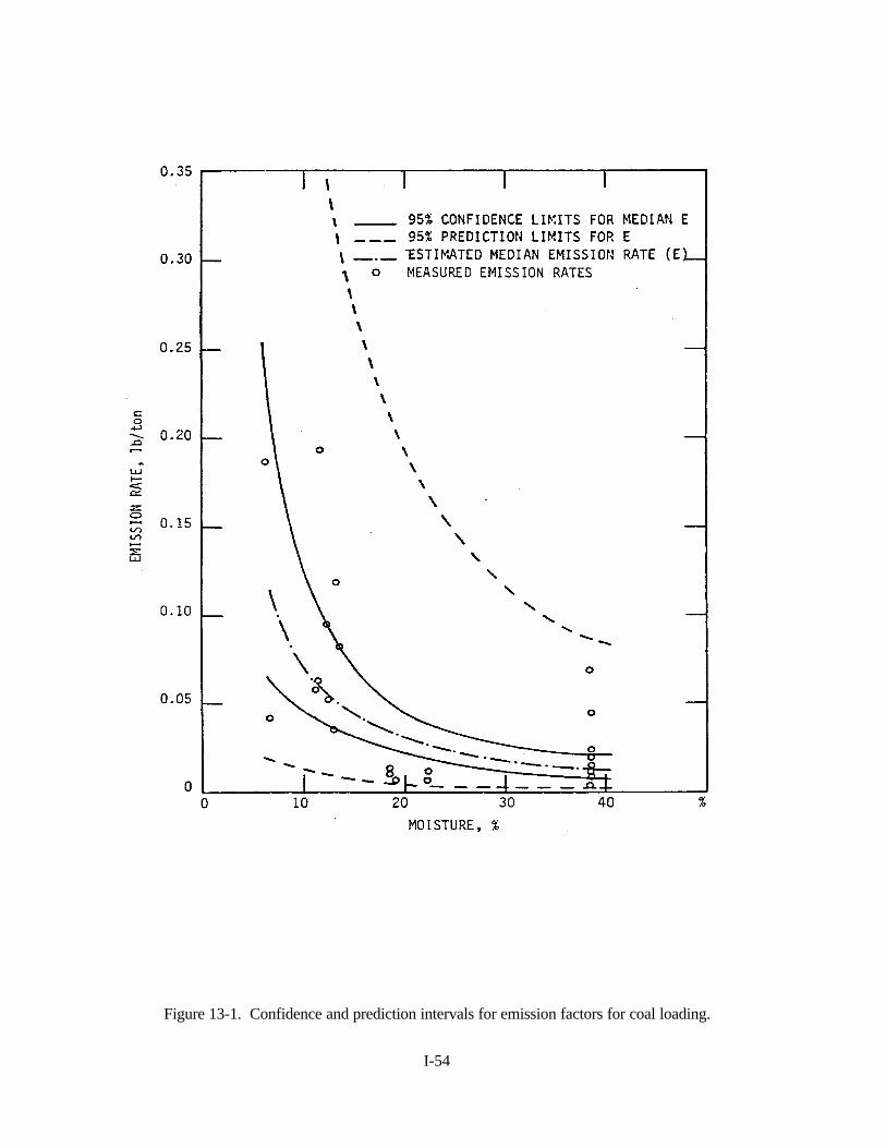
I-54
Figure 13-1. Confidence and prediction intervals for emission factors for coal loading.
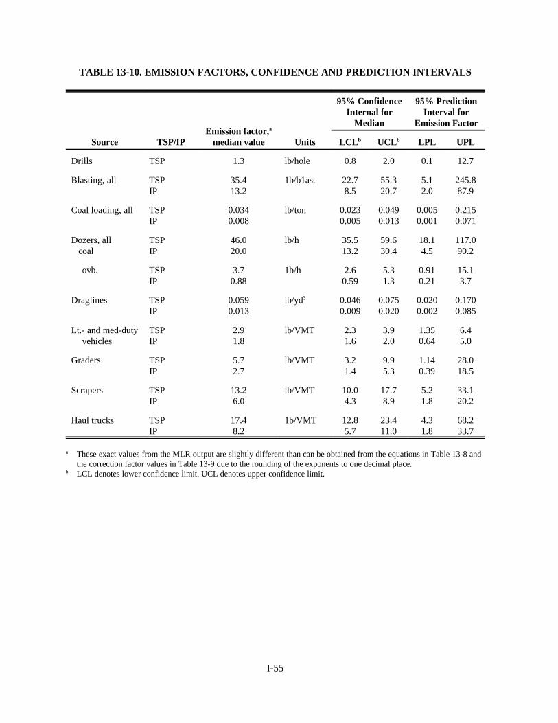
I-55
TABLE 13-10. EMISSION FACTORS, CONFIDENCE AND PREDICTION INTERVALS
Source TSP/IPEmission factor,a
median value Units
95% ConfidenceInternal for
Median
95% PredictionInterval for
Emission Factor
LCLb UCLb LPL UPL
Drills TSP 1.3 lb/hole 0.8 2.0 0.1 12.7
Blasting, all TSPIP
35.413.2
1b/b1ast 22.78.5
55.320.7
5.12.0
245.887.9
Coal loading, all TSPIP
0.0340.008
lb/ton 0.0230.005
0.0490.013
0.0050.001
0.2150.071
Dozers, all coal
TSPIP
46.020.0
lb/h 35.513.2
59.630.4
18.14.5
117.090.2
ovb. TSPIP
3.70.88
1b/h 2.60.59
5.31.3
0.910.21
15.13.7
Draglines TSPIP
0.0590.013
lb/yd3 0.0460.009
0.0750.020
0.0200.002
0.1700.085
Lt.- and med-dutyvehicles
TSPIP
2.91.8
lb/VMT 2.31.6
3.92.0
1.350.64
6.45.0
Graders TSPIP
5.72.7
lb/VMT 3.21.4
9.95.3
1.140.39
28.018.5
Scrapers TSPIP
13.26.0
lb/VMT 10.04.3
17.78.9
5.21.8
33.120.2
Haul trucks TSPIP
17.48.2
1b/VMT 12.85.7
23.411.0
4.31.8
68.233.7
a These exact values from the MLR output are slightly different than can be obtained from the equations in Table 13-8 andthe correction factor values in Table 13-9 due to the rounding of the exponents to one decimal place.
b LCL denotes lower confidence limit. UCL denotes upper confidence limit.
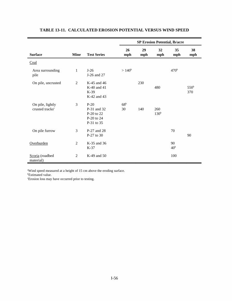
I-56
TABLE 13-11. CALCULATED EROSION POTENTIAL VERSUS WIND SPEED
Surface Mine Test Series
SP Erosion Potential, lb/acre
26mph
29mph
32mph
35mph
38mph
Coal
Area surroundingpile
1 J-26J-26 and 27
> 140b 470b
On pile, uncrusted 2 K-45 and 46K-40 and 41K-39K-42 and 43
230480 550b
370
On pile, lightlycrusted tracksc
3 P-20P-31 and 32P-20 to 22P-20 to 24P-31 to 35
68b
30 140 260130b
On pile furrow 3 P-27 and 28P-27 to 30
7090
Overburden 2 K-35 and 36K-37
9040b
Scoria (roadbedmaterial)
2 K-49 and 50 100
aWind speed measured at a height of 15 cm above the eroding surface.bEstimated value.cErosion loss may have occurred prior to testing.
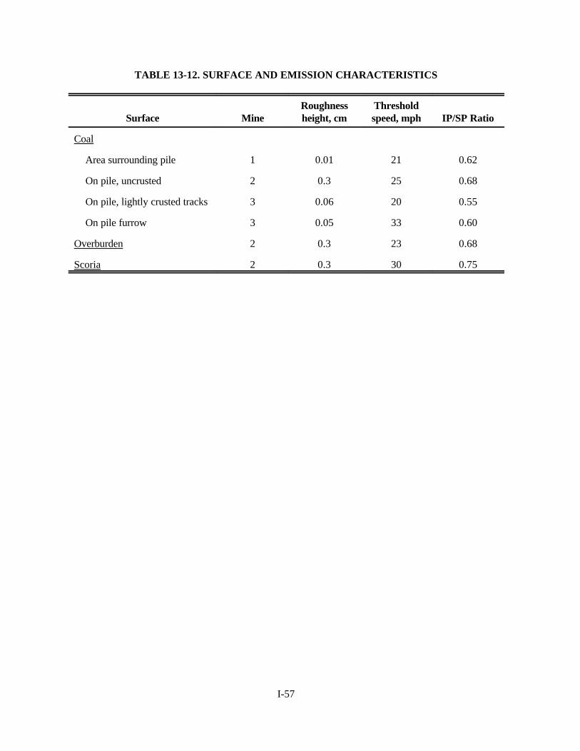
I-57
TABLE 13-12. SURFACE AND EMISSION CHARACTERISTICS
Surface MineRoughnessheight, cm
Thresholdspeed, mph IP/SP Ratio
Coal
Area surrounding pile 1 0.01 21 0.62
On pile, uncrusted 2 0.3 25 0.68
On pile, lightly crusted tracks 3 0.06 20 0.55
On pile furrow 3 0.05 33 0.60
Overburden 2 0.3 23 0.68
Scoria 2 0.3 30 0.75
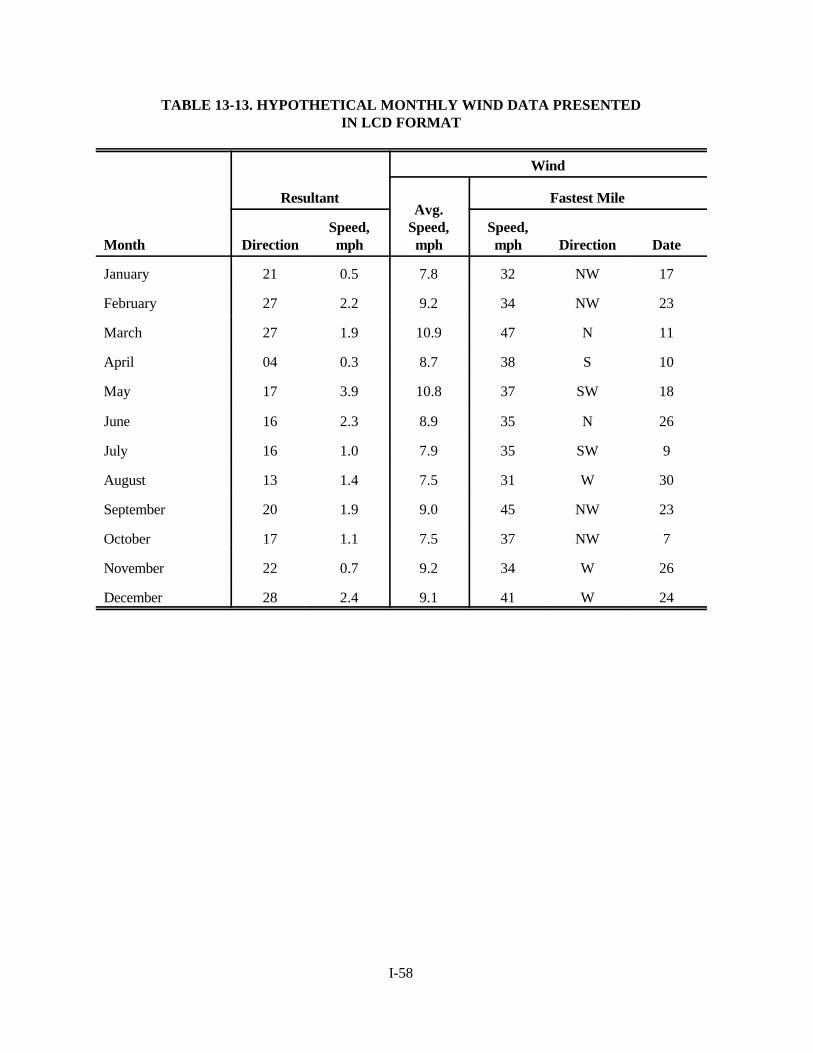
I-58
TABLE 13-13. HYPOTHETICAL MONTHLY WIND DATA PRESENTEDIN LCD FORMAT
Month
Resultant
Wind
Avg.Speed,mph
Fastest Mile
DirectionSpeed,mph
Speed,mph Direction Date
January 21 0.5 7.8 32 NW 17
February 27 2.2 9.2 34 NW 23
March 27 1.9 10.9 47 N 11
April 04 0.3 8.7 38 S 10
May 17 3.9 10.8 37 SW 18
June 16 2.3 8.9 35 N 26
July 16 1.0 7.9 35 SW 9
August 13 1.4 7.5 31 W 30
September 20 1.9 9.0 45 NW 23
October 17 1.1 7.5 37 NW 7
November 22 0.7 9.2 34 W 26
December 28 2.4 9.1 41 W 24

I-59
APPENDIX A
STEPWISE MULTIPLE LINEAR REGRESSION
Multiple linear regression (MLR) is a statistical technique for estimating expected values of a
dependent variable, in this case particulate emission rates, in terms of corresponding values of two or
more other (independent) variables. MLR uses the method of least squares to determine a linear
prediction equation from a set of simultaneously-obtained data points for all the variables. The equation
is of the form:
Emission rate Blxl + B2x2 + Bnxn + . . . + Bnxn + constant
where x1 to xn = concurrent quantitative values for each of the independent variables
B1 to Bn = corresponding coefficients
The coefficients are estimates of the rate of change in emission rates produced by each variable.
They can be determined easily by use of an MLR computer program or with a programmed calculator.
Other outputs of the MLR program are:
1. A correlation matrix. It gives the simple correlation coefficients of all of the variables
(dependent and independent) with one another. It is useful for identifying two interdependent
(highly correlated—either positive or negative) variables (two variables that produce the
same effect on emission rates), one of which should be eliminated from the analysis.
2. The multiple correlation coefficient (after addition of each independent variable to the
equation). The square of the multiple correlation coefficient is the fraction of total variance
in emission rates that is accounted for by the variables in the equation at that point.
3. Residual coefficient of variability. This is the standard deviation of the emission rates
predicted by the equation (with the sample data set) divided by the mean of the predicted
emission rates, expressed as a percent. If a variable eliminates some sample variance, it will
reduce the standard deviation and hence the relative coefficient of variability.
4. Significance of regression as a whole. This value is calculated from an F test by comparing
the variance accounted for by the regression equation to the residual variance. A 0.05
significance level is a 1 in 20 chance of the correlation being due to random occurrence.
5. Significance of each variable. This is a measure of whether the coefficient (B) is different
than 0, or that the relationship with the dependent variable is due to random occurrence.
Variables that do not meet a prespecified significance level may be eliminated from the
equation.

I-60
6. Constant in the equation.
The multiple correlation coefficient, unlike the simple correlation coefficient, is always positive
and varies from 0 to 1.0. A value of zero indicates no correlation and 1.0 means that all sample points lie
precisely on the regression plane. Because of random fluctuations in field data and inability to identify all
the factors affecting emission rates, the multiple coefficient is almost never zero even when there is no
real correlation and never 1.0 even when concentrations track known variables very closely. Therefore, it
is important to test for statistical significance .
The form of MLR in the program used in this study was stepwise MLR. Variables were added to
the equation in order of greatest increase in the multiple correlation coefficient, with concentrations then
adjusted for that variable and regressed against the remaining variables again. The procedure can be
ended by specifying a maximum number of variables or a minimum F value in the significance test. In
subsequent runs, the order of entry of variables was sometimes altered by specifying that a certain
variable be entered first or last.
In order to satisfy the requirement that the variables be quantitative, some were input as dummy
variables with only two possible values. For example, in an MLR run of all blasts, one variable had a
value of 0 for all coal blasts and 1 for all overburden blasts. The significance of this variable determined
whether there was a significant difference between coal and overburden blast emission rates, and the B
value was a direct measure of the difference between the two average emission rates after adjustment for
other variables in the MLR equation.
A statistically significant regression relationship between independent variables and particulate
emission rates is no indication that the independent variables cause the observed changes in emission rate,
as both may be caused by a neglected third variable.
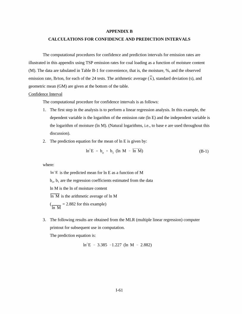
I-61
lnvE ' bo % b1 (ln M & ln M) (B-1)
lnvE & 3.385 &1.227 (ln M & 2.882)
APPENDIX B
CALCULATIONS FOR CONFIDENCE AND PREDICTION INTERVALS
The computational procedures for confidence and prediction intervals for emission rates are
illustrated in this appendix using TSP emission rates for coal loading as a function of moisture content
(M). The data are tabulated in Table B-1 for convenience, that is, the moisture, %, and the observed
emission rate, lb/ton, for each of the 24 tests. The arithmetic average ( ), standard deviation (s), andx
geometric mean (GM) are given at the bottom of the table.
Confidence Interval
The computational procedure for confidence intervals is as follows:
1. The first step in the analysis is to perform a linear regression analysis. In this example, the
dependent variable is the logarithm of the emission rate (ln E) and the independent variable is
the logarithm of moisture (ln M). (Natural logarithms, i.e., to base e are used throughout this
discussion).
2. The prediction equation for the mean of ln E is given by:
where:
is the predicted mean for ln E as a function of MlnvE
bo, b1 are the regression coefficients estimated from the data
ln M is the ln of moisture content
is the arithmetic average of ln Mln M
( = 2.882 for this example)ln M
3. The following results are obtained from the MLR (multiple linear regression) computer
printout for subsequent use in computation.
The prediction equation is:
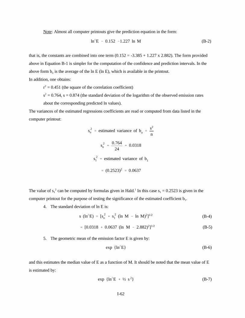
I-62
lnvE & 0.152 &1.227 ln M (B-2)
s 2o ' estimated variance of bo '
s2
n
s 2o '
0.76424
' 0.0318
s 21 ' estimated variance of b1
' (0.2523)2 ' 0.0637
' [0.0318 % 0.0637 (ln M & 2.882)2]1/2 (B-5)
s (lnvE) ' [s 2o % s 2
1 (ln M & ln M)2]1/2 (B-4)
exp {lnvE} (B-6)
exp {lnvE % ½ s 2} (B-7)
Note: Almost all computer printouts give the prediction equation in the form:
that is, the constants are combined into one term (0.152 = -3.385 + 1.227 x 2.882). The form provided
above in Equation B-1 is simpler for the computation of the confidence and prediction intervals. In the
above form bo is the average of the ln E (ln E), which is available in the printout.
In addition, one obtains:
r2 = 0.451 (the square of the correlation coefficient)
s2 = 0.764, s = 0.874 (the standard deviation of the logarithm of the observed emission rates
about the corresponding predicted ln values).
The variances of the estimated regressions coefficients are read or computed from data listed in the
computer printout:
The value of s12 can be computed by formulas given in Hald.1 In this case s1 = 0.2523 is given in the
computer printout for the purpose of testing the significance of the estimated coefficient b1.
4. The standard deviation of ln E is:
5. The geometric mean of the emission factor E is given by:
and this estimates the median value of E as a function of M. It should be noted that the mean value of E
is estimated by:

I-63
exp {lnvE ± t s(lnvE)} (B-8)
exp {lnvE ± 2.074 s(lnvE)} (B-8)
95% Limits{UCL ' 0.049 lb/tonLCL ' 0.023 lb/ton
exp {lnvE ± 1.321 s(lnvE)}
80% Limits{UCL ' 0.043 lb/tonLCL ' 0.027 lb/ton
exp {lnvE} ' 0.0339
Throughout the remainder of this discussion the GM values are used as estimates of the corresponding
median emission value.
6. The confidence interval for the median value of E as a function of M is obtained by:
where and s are obtained from Equations B-2 and B-4, respectively, and t is read for thelnvE (lnvE)
desired confidence level from a standard t table available in almost any statistical test (e.g., Hald's
tables2). Substituting values of M in Equation (B-8) (and B-2 and B-4) yields the results plotted in Figure
13-1 and repeated here for convenience as Figure B-1. One must not go beyond the limits for observed M
because there are no data or theory to support the extrapolation.
The 95 percent confidence limits for the median E at the GM of M (i.e., exp {2.882} = 17.85%)
are:
where
lnvE ' &3.385
s(lnvE) ' [0.0318 % 0.0637(0)]1/2 ' 0.178
and the upper (UCL) and lower (LCL) 95 percent confidence limits are:
Similarly, the 80 percent confidence limits are given by:
or
The median value is:

I-64
95% Limits{UCL ' 1.45 x predicated medianLCL ' 0.68 x predicted median
80% Limits{UCL ' 1.27 x predicted medianLCL ' 0.80 x predicted median
s (ln E) ' [s 2(lnvE) % s 2]1/2
' [s 2
n% s 2
1 (ln M & ln M)2 % s 2]1/2(B-9)
The above confidence limits are also expressed below as percentages of the predicted median, 0.0339.
These limits are a measure of the quality of the prediction of the median emission E for given M
on the basis of the data from the three mines. The widths of these confidence intervals are consistent with
data typically reported by EPA as stated in Section 15.
One application of these limits would be to estimate the median annual emissions based on a
large number of tons of coal loaded at the mine with GM moisture content of 17.85 percent. If the
moisture content deviates from this value (17.85%), it is necessary to calculate the interval at the
appropriate value of M using Equation (B-8 ) .
Because of the complication in presenting the complete results for all sources and pollutants as in
Figure B-1, the confidence intervals are presented only for the correction factors (M in this example) at
their GM value. Table 13-10 contains these data for all sources and pollutants.
Prediction Interval
The confidence interval previously described gives a measure of the quality of the data and of the
predicted median which is applicable only for a large number of operations relative to the emission factor
of interest. In the example in this appendix, this would imply a large number of coal loading operations
(or tonnage of coal loaded). There will be applications in which the number of operations is not large and
a prediction interval is desired which is expressed as a function of the number of operations. The
calculation of this interval follows the first three steps of that for the confidence interval; the subsequent
steps, starting with Step 4, are as follows:
4. The standard deviation of an individual predicted In emission factor is:

I-65
s (ln E) ' [0.0318 % 0.0637 (ln M & 2.882)2 % 0.764]1/2 (B-10)
exp {lnvE ± t s(ln E)}
exp {lnvE ± t[0.0318 % 0.0637 (ln M & 2.882)2 % 0.764]1/2} (B-11)
95% Limits{UPL ' 0.215 lb/tonLPL ' 0.005 lb/ton
80% Limits{UPL ' 0.110 lb/tonLPL ' 0.010 lb/ton
exp{lnvE ± t [s 2 (ln E) %s 2
N]1/2
} (B-12)
For the coal loading data,
5. The prediction interval for an emission factor E is
For the coal loading data, this interval is given by:
The results are plotted in Figure B-1 as a function of M. For the GM of M (i.e., ln M = 2.882),
the prediction limits are:
6. The prediction interval for an individual value is obviously much wider than the
corresponding confidence interval for a median value. If it is desired to predict the emissions
based on a number of operations, say N (e.g., N tons of coal), the confidence interval is
given by
that is, the last term in Equation B-9 is divided by N instead of 1. Note that as N becomes
large this result simplifies to that of Equation (B-8).
Test for Normality
One of the major assumptions in the calculations of the confidence and prediction intervals is that
the ln residuals (deviations of the ln E from ln E) are normally distributed, hence the lognormality
assumption for the original (and transformed data). A check for normality was performed on the ln
residuals for six data sets with the largest number of data values. In two of the six cases the data deviated
from normality (these two cases were TSP and IP emissions for Blasting). Based on these results, the
lognormal assumption was made because of both computational convenience and adequate
approximation for most of the data.
I-66
REFERENCES
1. Hald, A. Statistical Theory with Engineering Applications. John Wiley and Sons, Inc. New York. 1952.
2. Hald, A. Statistical Tables and Formulas. John Wiley and Sons, Inc. New York. 1952.
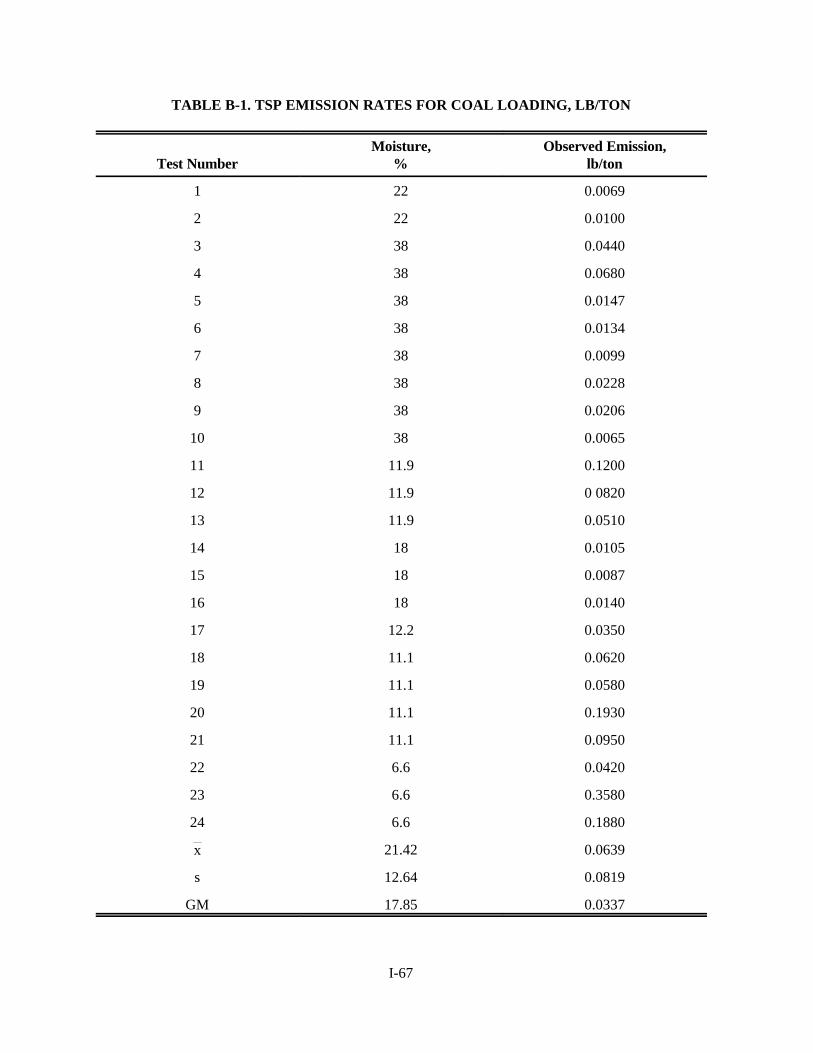
I-67
TABLE B-1. TSP EMISSION RATES FOR COAL LOADING, LB/TON
Test NumberMoisture,
%Observed Emission,
lb/ton
1 22 0.0069
2 22 0.0100
3 38 0.0440
4 38 0.0680
5 38 0.0147
6 38 0.0134
7 38 0.0099
8 38 0.0228
9 38 0.0206
10 38 0.0065
11 11.9 0.1200
12 11.9 0 0820
13 11.9 0.0510
14 18 0.0105
15 18 0.0087
16 18 0.0140
17 12.2 0.0350
18 11.1 0.0620
19 11.1 0.0580
20 11.1 0.1930
21 11.1 0.0950
22 6.6 0.0420
23 6.6 0.3580
24 6.6 0.1880
21.42 0.0639x
s 12.64 0.0819
GM 17.85 0.0337
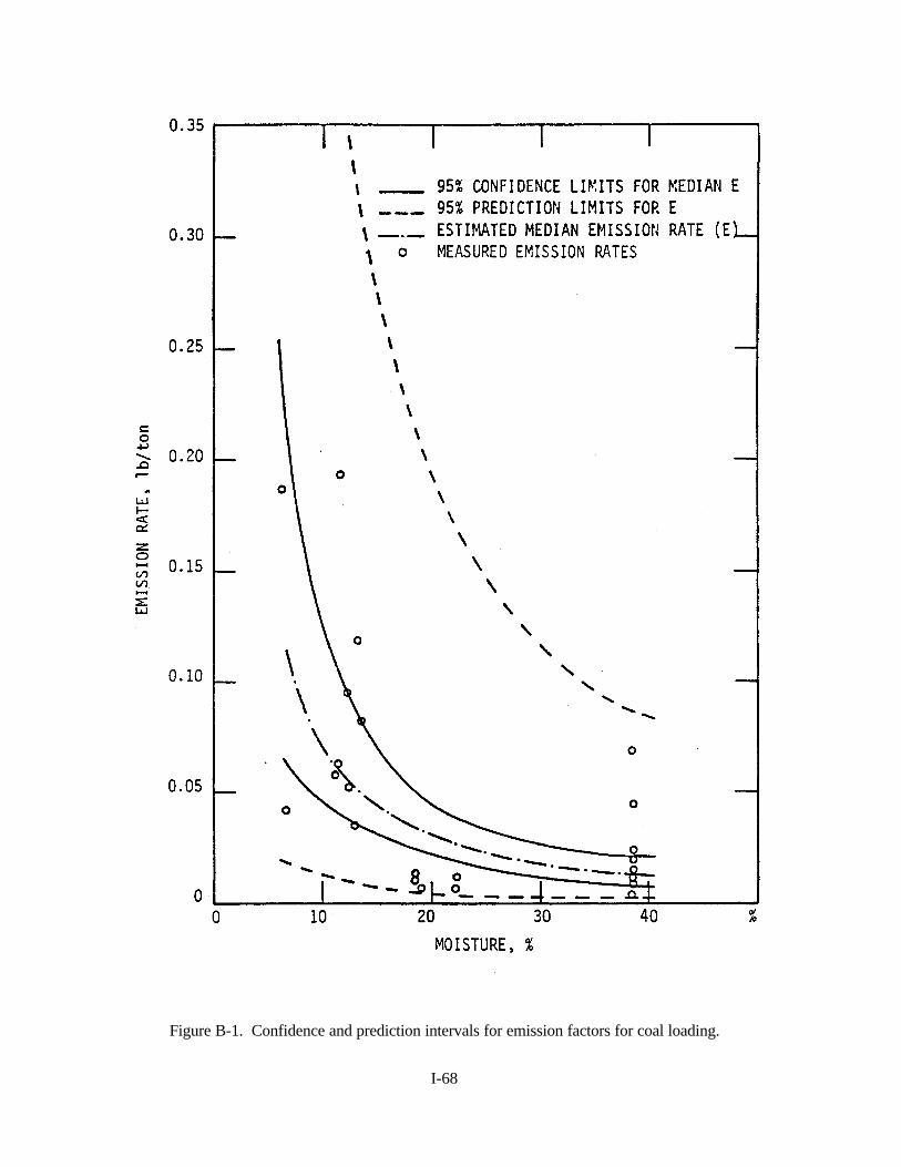
I-68
Figure B-1. Confidence and prediction intervals for emission factors for coal loading.


