
Cohort MortalityBy Rajeev Shah
CMIB UKCMIB, UK

StructureStructure
• The Continuous Mortality I i i B (CMIB)Investigation Bureau (CMIB)
• Two way mortality tablesTwo way mortality tables
• Cohort Effects

The CMIBThe CMIB
• Role• Features
Wh ffi t ib t d t• Why offices contribute data
NB “Office” = “company”ff p y

Role of the CMIBRole of the CMIB• Research – Mortality, IP and CI.y,
– Methodologies– GraduationGraduation– Models
D t ll ti• Data collection• Analysis & reporting
– Industry experience– Contributing officesg
• Standard Tables• Projecting future experience• Projecting future experience

Features of the CMIBFeatures of the CMIB
• Governed by the actuarial professionC ti i ti ti• Continuous investigations
• Independentp• Confidentiality is paramount
d d d li / /• Produce standard mortality/IP/CI tables
• Actuarial profession provides expertise

Why offices contribute data (1)Why offices contribute data (1)• Helps the market price and reserveHelps the market price and reserve
rationally– Provides confidence to regulators and consumers
h k i• Acts as a check on own assumptions– Comparison with industry experience and trendsComparison with industry experience and trends
– Small areas of experience e.g. Cause of Claim
• Benchmarking of underwriting/claims controlcontrol

Why offices contribute data (2)Why offices contribute data (2)
B fit f h d id• Benefit from new research and ideas– CMIB provides interface for exchange of ideas between
academia and the commercial world
Li it d d ti ithi ffi• Limited resources and expertise within offices
• Confidence in the CMIB and the actuarialConfidence in the CMIB and the actuarial profession
• Benevolent?t d t di d h– e.g. promote understanding and research

Standard mortality tablesStandard mortality tables
Period Assured Lives Annuitants Pensioners1924-29 (males)( )1947-48
1949 52 (males)1949-52 (males)1967-70 (males)
1975-78 (females)1979-82
1991-94

Comparison of the mortality of male assured livesComparison of the mortality of male assured livesComparison of the mortality of male assured livesComparison of the mortality of male assured lives400
300
350
250
300
f 196
7-70
150
200
cent
age
o
1924-291949-52
100
150
Perc
1967-70
1991 941979-82
0
501991-941979-82
17 22 27 32 37 42 47 52 57 62 67 72 77 82 87 92 97
Age
Two way mortality tables

Two way mortality tablesTwo way mortality tables
• Standard tables• Show mortality rates by age and
calendar yearcalendar year• Allow for projected mortality
improvements

T t bl f th b t blTwo way table for qx – the base table
Age 1992 1993 1994 1995 1996 1997 1998 1999 2000 2001 2002 2003 2004 20056061 C 1992C 199261626364
C=1992C=1992
65 66 67 68 69 70 71 72 72 73 74 75 7676 77

T t bl f f bi th 1935Two way table for qx- year of birth 1935
Age 1992 1993 1994 1995 1996 1997 1998 1999 2000 2001 2002 2003 2004 200560616162636465 66 67 68 69 70 71 72
B=1935B=193572 73 74 75 7676 77

T t bl f f 2000Two way table for qx – year of use 2000
Age 1992 1993 1994 1995 1996 1997 1998 1999 2000 2001 2002 2003 2004 200560 61 61 62 63 64 U=2000U=200065 66 67 68 69 70 71 72 72 73 74 75 7676 77

Cohort Effects

The problemThe problem
I h l li j i• Is the latest mortality projection (the “92” Series) still appropriate?(the 92 Series) still appropriate?
•If not, how should it change?

Pensioners 100A/E using the “92” Series projected mortality rates:Males
110110
100
tio
90
A/E
Rat
80 AmountsLi
100
701992 1993 1994 1995 1996 1997 1998 1999 2000
Lives
1992 1993 1994 1995 1996 1997 1998 1999 2000

Pensioners 100A/E using the “92” Series projected mortality g p j yrates: Males, lives, by age
66 - 70105
110
71 - 75
76 - 8095
100
atio
81 - 85
86 - 9085
90
95
0 A
/E R
a
91 - 9580
85
100
70
75
1992 1993 1994 1995 1996 1997 1998 1999

Cohort dataCohort data
• Assured lives 1947 to 1999A 10 t 100+• Age range 10 to 100+
• … 2-way table of qxy q• Pre 1974 data had to be entered manually
Ul i d i l• Ultimate durations only• Relatively homogeneousy g• Other data sets not as complete

SmoothingSmoothing
• Lots of attempts, but finallyt di i l li• … two dimensional splines
• Imposes no “shape” on the datap p• Smooth in two directions
f f i d• Lots of features in data• but difficult to see patterns in qxs… but difficult to see patterns in qxs
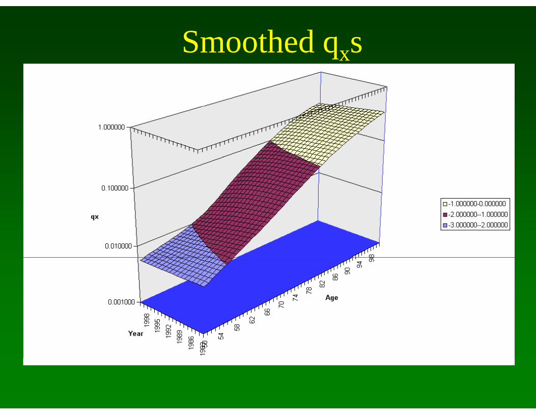
Smoothed qxsqx
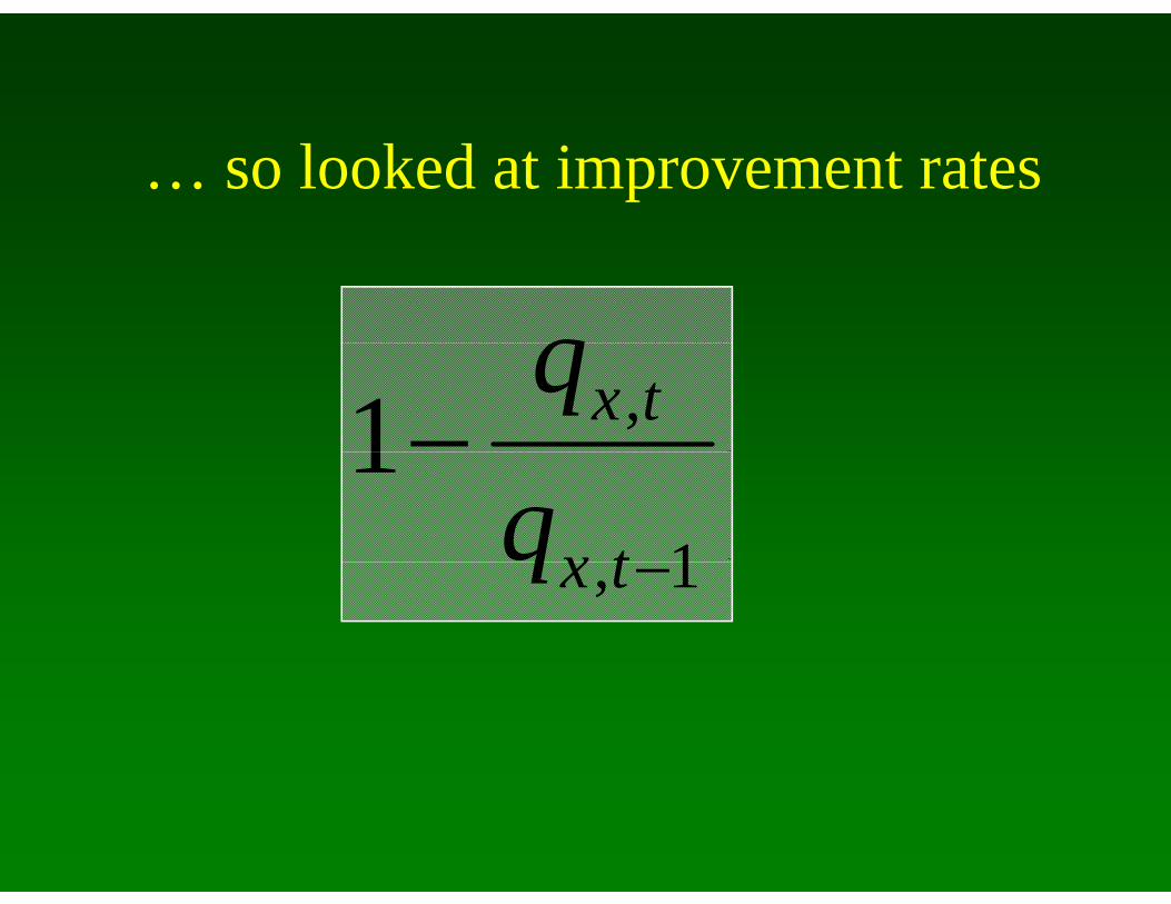
… so looked at improvement rates
q ,1 txq
1
1txq 1, txq

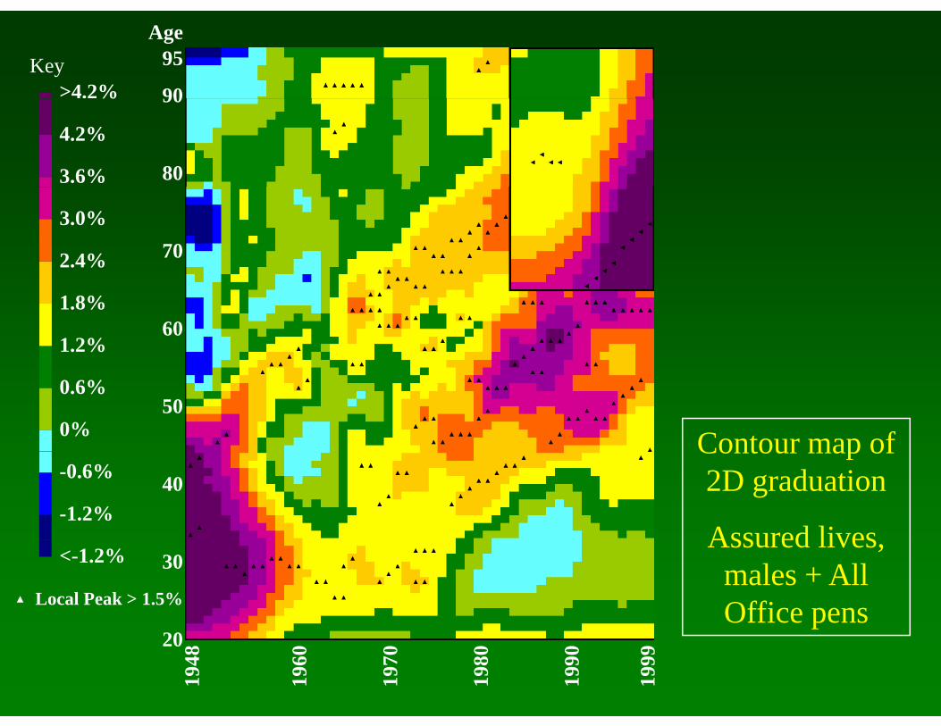
Improvement factorsp

95
90
AgeKey
>4.2%
80
90%
4.2%
3.6%
703.0%
2.4%
601.8%
1.2%
500.6%
0% Contour map of40-0.6%
-1.2%
Contour map of 2D graduation
Assured lives30
Local Peak > 1.5%
<-1.2%Assured lives,
males, all durations
20
1948
1960
1970
1980
1990
1999

Key>4.2%
95
90
Age
%
4.2%
3.6% 80
90
3.0%
2.4% 70
1.8%
1.2%60
0.6%
0%50 GAD Contour
map-0.6%
-1.2%40
map
Male Population<-1.2% 30Population, England &
Wales20
1948
1960
1970
1980
1990
1999
Wa es

Pensioner cohort dataPensioner cohort data
• 1983 – 1999 • Males, Females, Lives & Amounts• Data issues• Data issues• All Offices & Loyal Officesy• Males – improving more quickly than
A d LiAssured Lives

All Office Pensioners 100A/E using the “92” Series projected with Assured lives actual mortality improvements - Males
110110
100
tio
90
A/E
Rat
80 AmountsLi
100
A
701992 1993 1994 1995 1996 1997 1998 1999
Lives
1992 1993 1994 1995 1996 1997 1998 1999
95
90
AgeKey
>4.2%
80
90%
4.2%
3.6%
703.0%
2.4%
601.8%
1.2%
500.6%
0% Contour map of40-0.6%
-1.2%
Contour map of 2D graduation
Assured lives30
Local Peak > 1.5%
<-1.2%Assured lives,
males + All Office pens
20
1948
1960
1970
1980
1990
1999
p

95
90
AgeKey
>4.2%
80
90%
4.2%
3.6%
703.0%
2.4%
601.8%
1.2%
500.6%
0% Contour map of40-0.6%
-1.2%
Contour map of 2D graduation
Assured lives30
Local Peak > 1.5%
<-1.2%Assured lives, males + Loyal
Office pens20
1948
1960
1970
1980
1990
1999
p

All Office crude data to 1992 then “92” Series projectionAll Office crude data to 1992, then 92 Series projection
Crude Projection
100Age
C udedata Projection
90
80
61
70
61
< 1 2% 1 2% 0 6% 0% 0 6% 1 2% 1 8% 2 4% 3 0% 3 6% 4 2% <4 2%
1967
2040
1986
1992
2000
2010
2020
2030
1980
<-1.2% -1.2% -0.6% 0% 0.6% 1.2% 1.8% 2.4% 3.0% 3.6% 4.2% <4.2%

All Office to 1992, then “92” Series projection
Crude data Projection
Graduated data
, p j
100Age data Projectiondata
90
80
61
70
1967
2040
1983
1992
2000
2010
2020
2030
1980
61
< 1 2% 1 2% 0 6% 0% 0 6% 1 2% 1 8% 2 4% 3 0% 3 6% 4 2% <4 2%<-1.2% -1.2% -0.6% 0% 0.6% 1.2% 1.8% 2.4% 3.0% 3.6% 4.2% <4.2%

All Office to 83 - Loyal Office to 99 - then “92” Series
Crude d t Projection
Graduated d t
yprojection
100Age data Projectiondata
90
80
61
70
61
1967
2040
1983
1992
2000
2010
2020
2030
1980
< 1 2% 1 2% 0 6% 0% 0 6% 1 2% 1 8% 2 4% 3 0% 3 6% 4 2% <4 2%<-1.2% -1.2% -0.6% 0% 0.6% 1.2% 1.8% 2.4% 3.0% 3.6% 4.2% <4.2%

Sh t h tShort cohortCrude d t Projection
Graduated d t
100Age data Projectiondata
90
80
61
70
61
1967
2040
1983
1999
2010
2020
2030
1980
< 1 2% 1 2% 0 6% 0% 0 6% 1 2% 1 8% 2 4% 3 0% 3 6% 4 2% <4 2%<-1.2% -1.2% -0.6% 0% 0.6% 1.2% 1.8% 2.4% 3.0% 3.6% 4.2% <4.2%
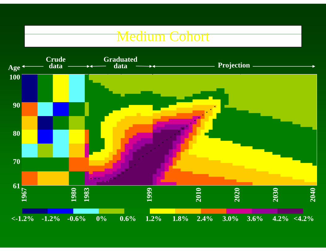
M di C h tMedium CohortCrude d t Projection
Graduated d t
100Age data Projectiondata
90
80
61
70
61
< 1 2% 1 2% 0 6% 0% 0 6% 1 2% 1 8% 2 4% 3 0% 3 6% 4 2% <4 2%
1967
2040
1983
1999
2010
2020
2030
1980
<-1.2% -1.2% -0.6% 0% 0.6% 1.2% 1.8% 2.4% 3.0% 3.6% 4.2% <4.2%

L C h tCrude d t Projection
Graduated d t
Long Cohort
100Age data Projectiondata
90
80
61
70
61
< 1 2% 1 2% 0 6% 0% 0 6% 1 2% 1 8% 2 4% 3 0% 3 6% 4 2% <4 2%
1967
2040
1983
1999
2010
2020
2030
1980
<-1.2% -1.2% -0.6% 0% 0.6% 1.2% 1.8% 2.4% 3.0% 3.6% 4.2% <4.2%

95
90
AgeKey
>4.2%
80
90%
4.2%
3.6%
703.0%
2.4%
601.8%
1.2%
500.6%
0% Contour map of40-0.6%
-1.2%
Contour map of 2D graduation
Assured lives30
Local Peak > 1.5%
<-1.2%Assured lives,
males + Medium Cohort
1948
1960
1970
1980
1990
1999
20

D i fi h 1992 99 d ?Does it fit the 1992-99 data?

All Office Pensioners 100A/E using the “92” Series projected with Medium Cohort improvement factors - Males
110110
100
tio
90
A/E
Rat
80 AmountsLi
100
A
701992 1993 1994 1995 1996 1997 1998 1999
Lives
1992 1993 1994 1995 1996 1997 1998 1999

Loyal Office Pensioners 100A/E using the “92” Series projected with Medium Cohort improvement factors - Males
110110
100
io
90
A/E
Rat
i
80 AmountsLi
100
A
701992 1993 1994 1995 1996 1997 1998 1999
Lives
1992 1993 1994 1995 1996 1997 1998 1999
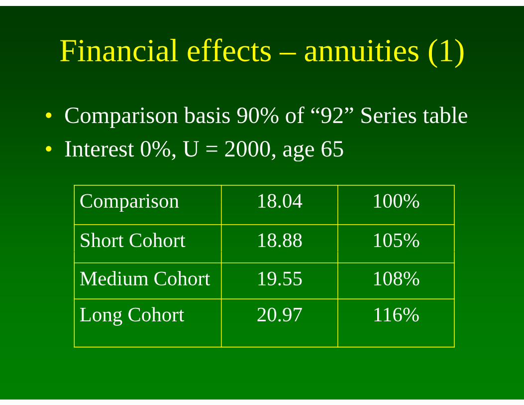
Financial effects – annuities (1)Financial effects annuities (1)
• Comparison basis 90% of “92” Series table• Interest 0% U = 2000 age 65Interest 0%, U 2000, age 65
Comparison 18 04 100%Comparison 18.04 100%
Short Cohort 18.88 105%
Medium Cohort 19.55 108%
Long Cohort 20.97 116%
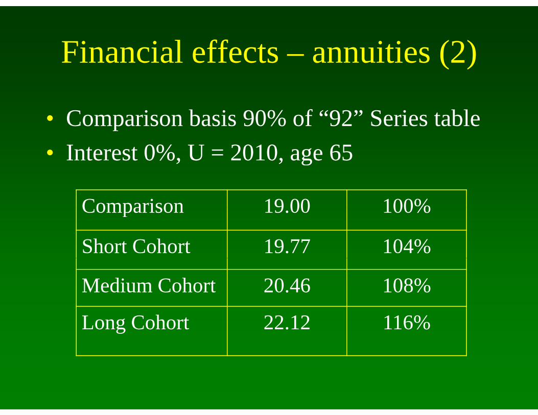
Financial effects – annuities (2)Financial effects annuities (2)
• Comparison basis 90% of “92” Series table• Interest 0% U = 2010 age 65Interest 0%, U 2010, age 65
Comparison 19 00 100%Comparison 19.00 100%
Short Cohort 19.77 104%
Medium Cohort 20.46 108%
Long Cohort 22.12 116%

Financial effects – annuities (3)Financial effects annuities (3)
• Comparison basis 90% of “92” Series table• Interest 3% U = 2000 age 65Interest 3%, U 2000, age 65
Comparison 13 08 100%Comparison 13.08 100%
Short Cohort 13.61 104%
Medium Cohort 13.94 107%
Long Cohort 14.58 112%

Financial effects – annuities (4)Financial effects annuities (4)
• Comparison basis 90% of “92” Series table• Interest 3% U = 2010 age 65Interest 3%, U 2010, age 65
Comparison 13 65 100%Comparison 13.65 100%
Short Cohort 14.14 104%
Medium Cohort 14.48 106%
Long Cohort 15.24 112%

Expectation of life for males aged 60 in 2000
a(55)M29
1999
1999 lc
a(55)M
PA(90)M
PMA8025
27
Life
1992
1999 mc
1999 sc
PMA92
PMA92mc23
25
ctat
ion
of L
1980
1992
PMA92lc
PMA92sc19
21
Expe
c
1955
1968
1970
1980
1990
2000
2010
2020
2030
17
1955
2 2 2 2

Things not yet doneThings not yet done
• Amounts v Lives• Males v Females• Males v Females• Graduate crude improvement factors• Comparison with other countries• Medical experts• Medical experts• Causes of death• Demography• Projection techniques (1 s d ?)• Projection techniques (1 s.d.?)

Where to get CMIB papers?Where to get CMIB papers?
www actuaries org ukwww.actuaries.org.uk
![[PPT]PowerPoint Presentationc.ymcdn.com/sites/ · Web viewDisclosures I, Rajeev Shah, DO NOT have a financial interest/arrangement or affiliation with one or more organizations that](https://cdn.vdocument.in/doc/165x107/5ae5f78c7f8b9a3d3b8c8c9e/pptpowerpoint-viewdisclosures-i-rajeev-shah-do-not-have-a-financial-interestarrangement.jpg)


