
Comparing
Two
Populations or
Groups10.1: part 2:
Comparing Two Proportions
Confidence Intervals

(Please grab a chromebook)Warm Up: Breakfast time
Researchers designed a survey to compare the
proportions of children who come to school
without eating breakfast in two low-income
elementary schools. An SRS of 80 students from
School 1 found that 19 had not eaten breakfast.
At School 2, an SRS of 150 students included 26
who had not had breakfast. More than 1500
students attend each school. Do these data
give convincing evidence at the 𝛼 = 0.05 level
of a difference in population proportions?
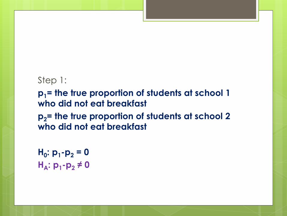
Step 1:
p1= the true proportion of students at school 1
who did not eat breakfast
p2= the true proportion of students at school 2 who did not eat breakfast
H0: p1-p2 = 0
HA: p1-p2 ≠ 0

Step 2 Solution If conditions are met, we should perform a two-
sample z test for the difference of proportions1. Random?
Yes
2. 10%:Sampling without replacement, so check:
80≤𝟏
𝟏𝟎𝟖𝟎𝟎 and 150≤
𝟏
𝟏𝟎𝟏𝟓𝟎𝟎
3. Large counts:
The counts of “successes” and “failures” in each sample or group are all at least 10
𝟏𝟗 ≥ 𝟏𝟎, 𝒂𝒏𝒅 𝟔𝟏 ≥ 𝟏𝟎𝟐𝟔 ≥ 𝟏𝟎, 𝒂𝒏𝒅 𝟏𝟐𝟒 ≥ 𝟏𝟎

Step 3 Solution
𝑛1 = 80Ƹ𝑝1 = 0.2375𝑛2 = 150Ƹ𝑝2 = 0.1733,
Ƹ𝑝1 − Ƹ𝑝2 = 0.0642Ƹ𝑝𝑐 = 0.1957
Test statistic: 𝒛 = 𝟏. 𝟏𝟕
P-value: 0.2427

Step 4 Solution
Because our P-value, 0.2427, is greater than
𝛼 = 0.05, we fail to reject the null hypothesis.
There is not convincing evidence that the
true proportions of students at the two
schools who didn’t eat breakfast are
different.

What IS the average difference between
the proportion of students from each
school who have not eaten breakfast?
To answer this, we will use a confidence
interval about a difference in proportions.

Conditions for constructing a
confidence interval about a
difference in proportions.1. Random?
The data come from two independent random samples or from two groups in a randomized experiment.
2. 10%:
When sampling without replacement, check that 𝒏𝟏 ≤𝟏
𝟏𝟎𝑵𝟏 and 𝒏𝟐 ≤
𝟏
𝟏𝟎𝑵𝟐
Do NOT need to check 10% in an experiment (unless the individuals are randomly sampled).
3. Large counts:
The counts of “successes” and “failures” in each sample or group are all at least 10
𝒏𝟏ෝ𝒑𝟏 ≥ 𝟏𝟎, 𝒂𝒏𝒅 𝒏𝟏(𝟏 − ෝ𝒑𝟏) ≥ 𝟏𝟎𝒏𝟐ෝ𝒑𝟐 ≥ 𝟏𝟎, 𝒂𝒏𝒅 𝒏𝟐(𝟏 − ෝ𝒑𝟐) ≥ 𝟏𝟎

Proceeding with Confidence
Intervals
Because we do not know the values of the
parameters p1and p2 in the standard
deviation formula, they are replaced by
Ƹ𝑝1 𝑎𝑛𝑑 Ƹ𝑝2. The result is the standard error of
the statistic, Ƹ𝑝1 − Ƹ𝑝2.
𝑺𝑬ෝ𝒑𝟏−ෝ𝒑𝟐 =ෝ𝒑𝟏(𝟏 − ෝ𝒑𝟏)
𝒏𝟏+ෝ𝒑𝟐(𝟏 − ෝ𝒑𝟐)
𝒏𝟐
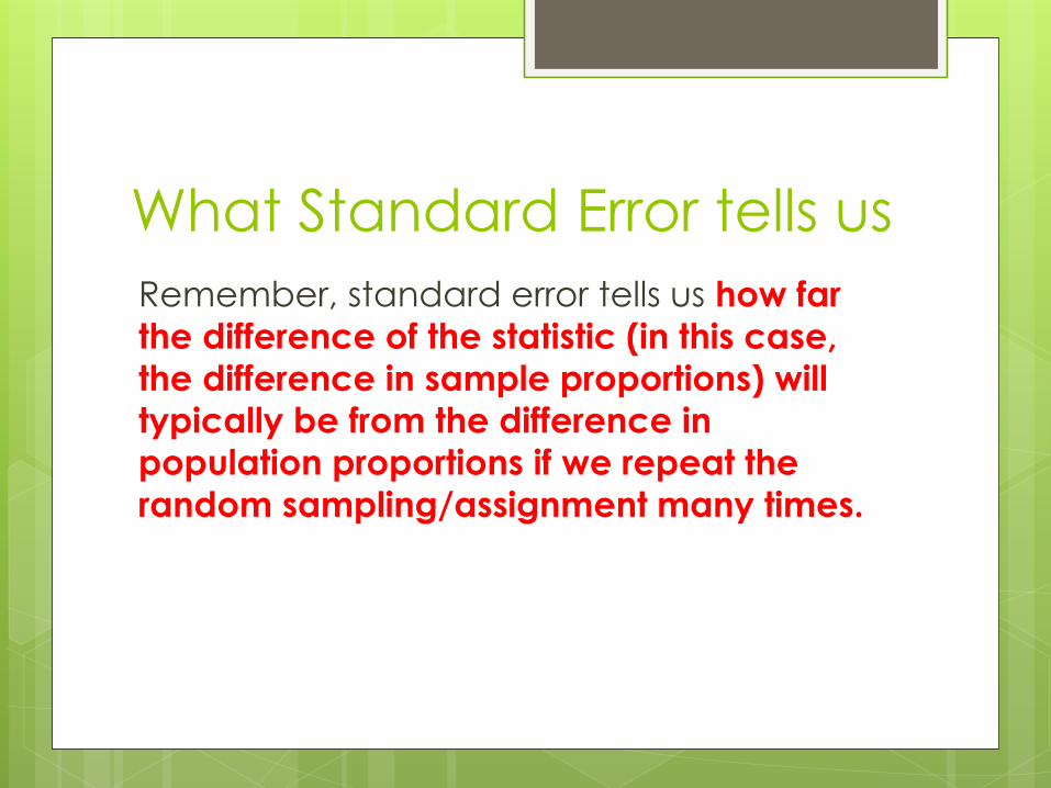
What Standard Error tells us
Remember, standard error tells us how far
the difference of the statistic (in this case,
the difference in sample proportions) will
typically be from the difference in
population proportions if we repeat the
random sampling/assignment many times.

Confidence interval for p1- p2
The format is still
Statistic ± (critical value) × (standard error)
( Ƹ𝑝1− Ƹ𝑝2) ± 𝒛ෝ𝒑𝟏(𝟏 − ෝ𝒑𝟏)
𝒏𝟏+ෝ𝒑𝟐(𝟏 − ෝ𝒑𝟐)
𝒏𝟐
Ending interval should look like…
< 𝑝1 − 𝑝2 <

Example 1
Back to the Breakfast problem
Construct the confidence interval for the true
difference in proportions of students between
School 1 and School 2 who did not have
breakfast on a given morning.
We are 95% that the interval from -0.047 to 0.175
captures the true difference in proportions of
students from School 1 and School 2 who did
not have breakfast on a given morning.

Significance test conclusions
and confidence intervalsWe are always looking for zero in the confidence interval.
• If zero is in the confidence interval, this means that there isn’t a significant difference between the proportions of two populations. The null hypothesis should have failed to be rejected.
• If zero is not in the confidence interval, this means that there is a significant difference between the proportions of two populations. The null hypothesis should have been rejected.
• An interval bound by two negatives tells us that the second population’s proportion was larger than the first.
• An interval bound by two positives tells us that the first population proportion was larger.
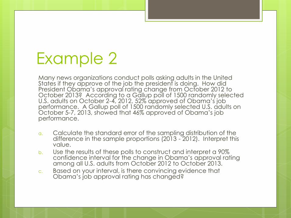
Example 2Many news organizations conduct polls asking adults in the United States if they approve of the job the president is doing. How did President Obama’s approval rating change from October 2012 to October 2013? According to a Gallup poll of 1500 randomly selected U.S. adults on October 2-4, 2012, 52% approved of Obama’s job performance. A Gallup poll of 1500 randomly selected U.S. adults on October 5-7, 2013, showed that 46% approved of Obama’s job performance.
a. Calculate the standard error of the sampling distribution of the difference in the sample proportions (2013 - 2012). Interpret this value.
b. Use the results of these polls to construct and interpret a 90% confidence interval for the change in Obama’s approval rating among all U.S. adults from October 2012 to October 2013.
c. Based on your interval, is there convincing evidence that Obama’s job approval rating has changed?

Another simulation

Penguin StudyAre metal bands used for tagging harmful to penguins? Researchers (Saraux et al., 2011) investigated this question with a sample of 20 penguins near Antarctica. All of these penguins had already been tagged with RFID chips, and the researchers randomly assigned 10 of them to receive a metal band on their flippers in addition to the RFID chip. The other 10 penguins did not receive a metal band. Researchers then kept track of which penguins survived for the 4.5-year study and which did not.

a. Identify and classify the
explanatory and response variables in this study.Explanatory:
whether or not the penguins were
“banned”
Response:
Did the penguin survive or not

b. Why did the researchers
include a comparison group in
this study?
Why didn’t they just see how
many penguins survived while
wearing a metal band?

c. Is this an observational
study or an experiment?
Explain how you know.

Hypothesis TestLet pm= the proportion of penguins who survived from the metal-band group.Let pc= the proportion of penguins who survived from the control group.
Ho: the survival rate of the banned penguins was the same as those without bands:
pm - pc = 0
HA: the survival rate of the banned penguins was less than those without bands:
pm - pc< 0

Results
No metal band (control)
Metal band Total
Survived 6 3 9
Did not survive 4 7 11
Total 10 10 20
The researchers found that 9 of the 20 penguins
survived, of whom 3 had a metal band and 6 did
not.
Complete the table.

Is it possible that this difference could have happened even if the metal band had no
effect; i.e., simply due simply to the random
nature of assigning penguins to groups (i.e.,
the luck of the draw)?
Sure, this is possible. But how unlikely is it? In order to answer this question we will once again turn to simulation. Like always, we will perform our simulation assuming that the null hypothesis is true: that the metal band has no effect on penguin survival. More specifically, we will assume that the 9 penguins who survived would have done so with the metal band or not, and the 11 penguins who did not survive also would have not survived with the metal band or not. This situation is too complex to be modeled by flipping a coin, but we can use cards.

Simulatione) You will need 20 cards: 10 black, 10 red. The black cards will represent the penguins who would have died no matter if they had a metal band or not, and the red cards would represent the penguins who would have lived no matter what.
f) Perform this shuffling and dealing. Then fill in the table of simulated results in the table.g) Calculate the difference in proportions who survived (control minus metal band group).
h) Repeat this shuffling and dealing a second time. Again fill in the table of simulated results:i) Calculate the difference in proportions who survived (control minus metal band group):
j) Plot both of your difference in proportions on a constructed dotplot of the differences in success proportions (control minus metal band group). Be careful to label the axis clearly and correctly.

Using the Applet We really need to carry out this simulated random assignment process hundreds, preferably thousands of times. This would be very tedious and time-consuming by hand, so let’s turn to the Two Proportions applet found at: http://www.rossmanchance.com/ISIapplets.html.
l) Enter the observed counts in the 2×2 table for this study into the table in the upper left cell of the applet.
• Click: Use Table
• Check the Show Shuffle Options and then press the Shufflebutton.
• Check the Show table box on the
• Press the Shuffle more times.
• Increase the Number of Shuffles so that the applet “shuffles” at least 1000 total hands.

m) Describe the resulting (null) distribution of
the differences in sample proportions of
survival between the two groups.
Comment on its shape (does this look
familiar), center (why does the center make
sense?), and variability.

n) Determine the proportion of your 1000 simulated random assignments for which the results are at least as extreme as the actual study (which, you’ll recall, saw a 0.30 difference in success proportions between the groups). Report and interpret this (approximate) p-value, including what is meant by the phrase “by chance alone” in this context.
The P-value describes how common the study’s actual difference in penguin survival rate is, assuming that there is no difference in survival rates between the banned and non-banned penguins; it describes how often the results from the study occurred by chance alone, with no influence of the bands on the survival rates.

o) Is your simulated p-value small enough so that you would consider a difference in the observed proportion of successes of 0.30 or more to be surprising under the null model that the metal band has no effect on penguins’ survival?
p) Explain why it would not be appropriate to conclude that this experiment provides strong evidence that the metal band has no effect on penguins’ survival.

Full Study We have a confession to make: The results described above were actually just a small part of the study. We chose to start with partial results to make the by-hand simulation with cards fairly manageable. But the actual study involved 100 penguins, with 50 randomly assigned to each group. The researchers found that 16 of 50 survived in the metal band group, and 31 of 50 survived in the control group.
q) Record the actual results from the full study in the 2×2 table:
r) Determine the conditional proportions who survived in each group. Also calculate the difference in these proportions (control – metal band). Is the value of this difference similar to what you calculated earlier for the partial study?
No metal band (control)
Metal band Total
Survived 31 16 47
Did not survive 19 34 53
Total 50 50 100

s) Describe how you could use cards to perform a simulation analysis based on data from the full study. Indicate what would be different from your earlier simulation analysis, and also indicate what would remain the same.
t) Use the applet to conduct a simulation analysis based on data from the full study. Conduct at least 1000 repetitions of the random assignment. Again describe the (null) distribution of the difference in conditional proportions of survival between the two groups (shape, center, variability).
u) Use the applet to determine the (approximate) p-value from your simulation analysis. Interpret what this p-value means in this context.


