comparing populations using sample statistics

Building Concepts: Comparing Populations Using

Sample Statistics TEACHER NOTES

©2016 Texas Instruments Incorporated 1 education.ti.com

Lesson Overview

In this TI-Nspire lesson, students compare two populations based on

samples of the same size from each population. Students use

measures of both center and spread to make informal inferences

about the difference between two populations.

Learning Goals

1. Make conjectures about

differences between two

populations based on samples

of the same size from those

populations;

2. recognize that measures of

both center and spread are

important in comparing the

means from two different

samples;

3. recognize that as the sample

size increases, the variability in

the difference of means or

difference in medians

decreases.

Measures of center and spread are useful in comparing two

random samples of the same size from different

populations.

Prerequisite Knowledge Vocabulary

Comparing Populations using Sample Statistics is the twenty-first

lesson in a series of lessons that explore the concepts of statistics

and probability. In this lesson students compare two populations

and make informal inferences about the difference between them.

This lesson builds on the concepts of the previous lessons. Prior to

working on this lesson students should have completed Tables

and Measures of Center and Spread, and Sample Means.

Students should understand:

• how to find and interpret measures of central tendency;

• that random sampling is likely to produce a sample that is

representative of the population;

• how sample size affects the spread of a sampling distribution of

sample means.

mean: the sum of all the data

values in a set of data divided by

the number of data values

median: the value that

separates the upper half of the

distribution of a set of data

values from the lower half

interquartile range: the

difference between the upper

quartile and the lower quartile

mean absolute deviation: the

mean of the absolute values of

all deviations from the mean of

a set of data

random sample: sample in

which every possible

combination of sample size n

from the population has the

same chance of being selected.




Lesson Pacing

This lesson should take 50–90 minutes to complete with students, though you may choose to extend, as

needed.

Lesson Materials

Compatible TI Technologies:

TI-Nspire CX Handhelds, TI-Nspire Apps for iPad®, TI-Nspire Software

Comparing Populations using Sample Statistics_Student.pdf

Comparing Populations using Sample Statistics_Student.doc

Comparing Populations using Sample Statistics.tns

Comparing Populations using Sample Statistics_Teacher Notes

To download the TI-Nspire activity (TNS file) and Student Activity sheet, go to

http://education.ti.com/go/buildingconcepts.

Class Instruction Key

The following question types are included throughout the lesson to assist you in guiding students in their

exploration of the concept:

Class Discussion: Use these questions to help students communicate their understanding of the

lesson. Encourage students to refer to the TNS activity as they explain their reasoning. Have students

listen to your instructions. Look for student answers to reflect an understanding of the concept. Listen for

opportunities to address understanding or misconceptions in student answers.

Student Activity: Have students break into small groups and work together to find answers to the

student activity questions. Observe students as they work and guide them in addressing the learning goals

of each lesson. Have students record their answers on their student activity sheet. Once students have

finished, have groups discuss and/or present their findings. The student activity sheet can also be

completed as a larger group activity, depending on the technology available in the classroom.

Deeper Dive: These questions are provided for additional student practice and to facilitate a deeper

understanding and exploration of the content. Encourage students to explain what they are doing and to

share their reasoning.

http://education.ti.com/go/buildingconcepts




Mathematical Background

The lessons Sample Proportions and Sample Means deal with finding measures of center for proportions

and for means. Many of the practical problems dealing with measures of center involve comparing two or

more groups, such as comparing average scores for males and females or comparing average time spent

on homework by sixth grade students and by eighth grade students. Such comparisons may involve

making conjectures about population characteristics (parameters) and constructing arguments based on

sample data to support the conjectures; for example, does the difference between the means of samples

from two populations provide convincing evidence that the means of the two populations also differ?

Graphical representations can show how two samples vary. Constructing sampling distributions of a

sample mean using simulations can show how much the sample mean varies between the two

populations. Two simulated sampling distributions that have a small amount of variability and little overlap

provide some evidence of a real difference between the two population means. If the overlap of the two

distributions is more substantial, the evidence is weaker for declaring that a difference between the

populations exists. This can be confirmed by investigating the numerical difference between the two

sample means. If there is no difference between two population means you would expect a simulated

sampling distribution of the differences to center around 0; if there is a difference, you would expect the

distribution to cluster around the actual difference, some value greater or less than 0. In later work, this

process is quantified, but in this lesson, students just explore the notion of a difference in a general way.




Part 1, Page 1.3

Focus: Measures of center and variability

from random samples can be useful in

drawing informal comparative inferences

about two populations.

Page 1.3 shows the distribution of two

samples each of size 20 from data about the

number of hours a week middle school

students in a large city spend doing

homework.

TI-Nspire

Technology Tips

b accesses

page options.

e cycles through

bins in the

histograms.

· takes new

data.

Up/Down arrows

move between

distributions.

/. resets the

page.

Sample generates new random samples.

Measures shows the intervals mean+/-MAD and IQR on the distributions.

The arrow keys on the screen or handheld change the sample size.

Selecting a bar displays the domain of the bar.

Reset returns to the original two distributions.

Class Discussion

These questions engage students in thinking about how to compare two different random samples

by looking at a histogram of each sample chosen from two different populations and considering

measures of center and spread. Note that the original samples on page 1.3 are the same for every

student, but the sample command generates random samples so all students will have different

samples.

Page 1.3 shows the distribution of two samples, each of size 20 from data about the number of

hours a week middle school students in a large city spend doing homework.

Have students… Look for/Listen for…

Make a conjecture about whether you think

there is a difference in the number of hours

boys and girls spend per week on

homework.

Answers will vary. It may appear that girls do

more homework than boys.




Class Discussion (continued)


Select menu> Measures> Mean +/- MAD. Do

the intervals determined by the mean +/-

MAD support your conjecture?

Answers may vary. From the samples on page

1.3, it appears that the girls do more homework

than the boys, with the mean number of hours

1.6 hours apart (6.8 to 5.6 hours). The intervals

have some overlap, but not enough to cause us

to question our conjecture. The interval for the

mean absolute deviation goes from about 1

54

hours to about 1

84

hours for the girls and from

about 4 hours to 1

62

hours for the boys.

Select menu> Measures> LQ, Median, UQ.

Do these measures support your

conjecture?

Answer: It looks like girls do more hours of

homework per week than boys since nearly half

of the girls do more hours of homework than

three fourths of the boys. Also, it looks like 75%

of the girls do more hours of homework than 50%

of the boys. The IQR for the boys is larger at

about 3 hours and shifted to the left, from 1

32

to

16

2 hours, while the IQR for the girls was

smaller at about 1

22

hours, from 1

52

to almost 8

hours.

Generate another two samples of size 20 selected

from the same population of seventh graders.

Do these new samples support your

conjecture about the difference in boys and

girls and the number of hours per work they

do homework?

Answers will vary as the samples are randomly

generated. In one set of samples, the number of

hours girls spent doing homework was more

variable than the number of hours boys did

homework. However, the mean and median

hours of homework for the girls were both about

two hours more than the mean and median for

the boys (1

52

hours to 1

74

hours); 75% of the

girls did more hours of homework than 50% of

the boys. These also support the conjecture.





Select several more samples of size 20.

Based on these samples do you think there

is evidence that boys spend less time on

homework than girls?

Answers will vary. A typical response might be

that it is really hard to tell as sometimes the

intervals for mean +/-MAD overlap a lot with the

interval determined by the LQ and UQ and

sometimes they don’t.

Why is it important to look at the distribution

of hours per week both boys and girls spend

doing homework rather than using only the

measures of center for the distributions?

Make a sketch to support your reasoning.

Answers will vary. You need to know how the

data are spread out; suppose the distributions

are relatively mound shaped and symmetric, and

the mean of one was 5 and of the other was 8. If

the ranges for each were very small, i.e. if the

first went from 3.5 to 6.5 and the second from 8

to 10, the two distributions would not overlap at

all and would seem to be samples from

populations with a distinct difference in center. If

the interval for mean+/- MAD of the first went

from 0 to 10 and of the second from 4 to 12, the

distributions overlap and it would not be clear

whether they overlap by chance or due to a real

difference in the population.

Part 1, Page 1.5

Focus: Students use measures of center and

variability from random samples to draw

informal comparative inferences about two

populations.

On page 1.5, the data are random samples

of the number of hours boys and girls do

homework from another school in the

district.

TI-Nspire

Technology Tips

b accesses

page options.

e cycles through

buttons or bars on

the histogram.

· activates a

button.

Up/Down arrows

choose where tab

is active.

/. resets the

page.

Sample generates different random samples from two populations.

Measures shows the intervals mean +/-MAD and IQR on the distributions.

Show Histogram and Show Boxplot cycle between displaying the

distributions as box plots or as histograms.

New Pops generates random samples from new schools.

The arrow keys on the screen or handheld change the sample size.

Reset returns to the original two distributions.

Class Discussion




In these questions, students use box plots, histograms and summary measures to make conjectures

about whether the samples come from different populations.


Go to page 1.5. The data are random samples of

the number of hours boys and girls do homework

from another school in the district.

Do the two samples seem to show a

difference between the number of hours

boys and girls spend doing homework?

Explain your reasoning.

Answers will vary as the samples are randomly

generated. In one set of samples, 3

4 (75%) of

the girls spent more hours on homework than 3

4

of the boys, so the evidence clearly supports the

statement that girls in that school do more hours

of homework per week than boys.

Change the display to a histogram and

display the mean and the mean +/-MAD. Do

the histogram and the measures of center

and spread support your thinking from the

question above?

Answers will depend on student distributions. For

the sample used above: Yes, most of the girls

seem to spend more time doing homework than

the boys do. The measures of center are 2.6

hours apart (7.4 mean hours for the girls and 4.8

mean hours for the boys; 7.1 median hours for

the girls and 4.5 hours for the boys) and the

intervals determined by the mean +/-MAD do not

overlap, while the intervals determined by the

IQR overlap by only about an hour.

Generate several more random samples of

the number of hours of homework for boys

and for girls from this school. Do the

samples provide evidence that boys and

girls are different with respect to how much

time they spend doing homework? Explain

why or why not.

Answers will depend on student distributions. For

the sample used in the first question: Yes boys

and girls seem to be different with respect to how

much homework they do because typically the

samples show that at least 3

4 of the girls spend

more hours doing homework than 3

4 of the boys

spend. The measures of center are usually at

least 2.5 hours apart, and the intervals

determined by the IQR and the mean +/-MAD

often do not overlap.






Work with a partner and use New Pops to

generate several random samples of students

from another school in the district. Do these

samples provide evidence that boys and girls at

that school are different with respect to how

much time they spend doing homework?

Explain why or why not.

Answers will vary because the populations are

randomly generated. In some cases, the

difference between the measures of center will

typically greater than one MAD, and the boys are

consistently doing more homework than the girls.

This would indicate a difference. Other students

may observe little difference in the measures of

center, and it could vary from sample to sample

whether boys or girls do more homework. In this

case students should say there isn’t evidence of

a difference.

Repeat the problem above with random samples

from three or four other schools in the district,

i.e., other populations. Be ready to share your

thinking with the class.

Answers will vary because populations are

randomly generated. Be sure responses are

comparing centers in terms of measures of

spread and overlap of the distributions. Thinking

about what you can say about how boys and girls

in the top or bottom half of the distributions

compare will be helpful.

Part 2, Pages 2.2 and 2.3

Focus: Simulated sampling distributions of the

differences in sample means can be used to

develop a sense of variability in sample

differences when making comparison between

population means.

The commands on pages 2.2 and 2.3

function in the same way as those on

page 1.3.

Selecting points on the sampling distribution

of differences displays the sample

distributions that generated that point.

Note: after the first 10 samples, Sample

generates 10 sample differences at a time.

TI-Nspire

Technology Tips

b accesses

page options.

e cycles

between bins on

each distribution or

between points on

the number line.

Up/Down arrows

choose where tab

is active.

/. resets the

page.




Class Discussion

Teacher Tip: In the following series of questions students consider the distributions

of the two samples and generate simulated sampling distributions of the statistic, the

difference, to compare two populations, boys and girls, with respect to the number of

hours doing homework per week. This first set of questions explores two random

samples where the evidence from the simulated distributions suggests there is a

difference in the means of the two populations.

In these questions, students consider a statistic calculated from two samples, the difference in

sample means.

One of the strategies in statistics is to find a

numerical way to quantify observations. Which of

the following might be useful to see whether two

samples came from populations with the same

characteristics? Explain your reasoning.

a. The difference between the length of the

intervals formed by the mean +/- MAD and

the IQR

b. The difference between the ranges of each

sample

c. The difference between the means of each

sample

d The difference between the medians of each

sample

Answers will vary. While a and b give measures

of spread, the measures are not anchored to a

position and so just finding the differences

between the lengths would not give indication of

how the centers compare. Either c or d might be

useful in at least knowing about the difference in

a measure of center.

Go to page 2.2. The samples are randomly drawn

from surveys given to students in schools in a

different district.





Describe the distributions of the number of

hours boys in the sample spend doing

homework and the number of hours girls in

the sample spend doing homework. Use the

intervals represented by the IQR (or mean +/-

MAD) to support your thinking.

The first sample is the same after that, samples

will vary randomly.

Answer: The sample of girls has more variability

in the number of hours they spend doing

homework than the sample of boys. (Note, the

range is larger for the girls than for boys as is the

IQR.) The mean number of hours both boys and

girls spent doing homework was close to 6 hours

per week. 75% of both the boys and the girls

spend at least 4.5 hours a week on homework

although the top 25% of the girls spend more

than 8 and up to 11 hours per week on

homework, while the top 25% of the boys spend

between 7 and 8 hours per week.

The dot on the number line on the right of

the page has a value .0 7 . What does the

number .0 7 tell you?

Answer: 0.7 is the difference between the

mean number of hours spent on homework for

the sample of 20 boys minus the mean number

of hours spent on homework for the sample of 20

girls. Thus, the girls spent about 7

10of an hour

more doing homework than boys.

Does the difference in the samples seem to

indicate a real difference in the mean

number of hours per week boys and girls

spent on homework?

Answers may vary. It does not seem like there is

a real difference. The means are pretty close

together, and there is quite a lot of overlap

between the two sample distributions, although

the girls do have more variability in the number of

hours doing homework than boys.

Teacher Tip: In the following questions students explore random samples where the

evidence suggests there is not a difference in the means of the two populations

sampled. Students should compare their simulated sampling distributions of the

differences in sample means when answering the last question in this series and note

that the simulated distributions in means for the samples from the populations on

page 2.2 have very similar shapes, centers and spreads as do the simulated

sampling distributions of the differences in means for samples from the populations

on page 2.3.





Generate two other samples.

What is the difference between the means

for each of these two samples? Looking at

the distributions of the two samples, would

you say there was a difference between the

number of hours per week boys and girls

typically spend doing homework?

Answers will vary because the samples are being

randomly generated. In one case the differences

were 1.6 hours and 2.6 hours. There still

appears to be a lot of overlap between the two

sample distributions, but in each case the girls

have spent more time doing homework, on

average, than the boys have.

Generate 20 random samples. What do you

notice about the simulated distribution of

the differences in the sample means?

Interpret your answer in terms of the

number of hours boys and girls spend doing

homework.

Answer: All of the differences seem to be

negative. The sampling distribution is boy mean –

girl mean, so a negative difference indicates that

the girls have a greater mean number of hours

doing homework. Fairly consistently, the

distributions show that 75% of the girls do more

homework than 25% or 50% of the boys, e.g.,

75% of the girls but only 25% of the boys do more

than 6.5 hours of homework per week.

Generate about 100 samples. Did any

simulation ever have boys doing more

homework than the girls, on average?

Explain your reasoning.

Answers may vary. If boys did more homework on

average, then the difference in the sample means

would be positive. None of the differences in the

simulated sampling distribution were positive.

Describe the simulated distribution of

sample differences. What would you

conclude about the number of hours spent

on homework by boys and by girls?

Answer: The simulated distribution is mound

shaped and relatively symmetric, with a center

around 2.5 hours. The range goes from about

4 to 0.7 hours. This distribution supports the

conjecture that girls do more hours of homework

than boys. No samples ever had the boys doing

more homework than the girls.




Student Activity Questions—Activity 1

1. Which of the following results is unlikely to occur by chance when sampling from this district?

Give an example from the TNS activity to support your reasoning.

Sample 1: Boys’ mean minus girls’ mean was 0.

Sample 2: Boys’ mean minus girls’ mean was 3 .


Sample 4 Boys’ mean minus girls’ mean was 0.5.

Answers may vary slightly due to random generation of samples. The simulated sampling distribution

should indicate that 0 and 0.5 are very unlikely to happen when sampling from this district. A

difference of 4 did not occur often, while a difference of 3 was common.

2. Go to page 2.3. These samples come surveys from students in another district.

a. Look at the distributions, then go to page 2.2 and Reset. How do the distributions on page

2.2 compare to the distributions on page 2.2?

Answer: The distributions are the same.

b. Go back to page 2.3 and generate 10 samples. Looking at the last two samples, would you

say there was a difference between the number of hours per week boys and girls typically

spend doing homework?

Answers may vary. In one case, the 10th sample had a difference in means of 0.4 which meant the

boys spent, on average, 0.4 hours more on homework than the girls. However, all of the boys

times were greater than the minimum girl time and less that the maximum girl time. This does not

indicate a difference in average time spent on homework for boys and girls in this district.

c. Did any simulation ever produce results where, on average, boys did more homework than

the girls? Explain your reasoning.

Answers may vary. If boys did more homework on average, then the difference in the sample

means would be positive. About half of the differences in the means were positive.

d. Generate at least 100 samples. Describe the simulated distribution of sample differences.

What would you conclude about the number of hours spent per week on homework by

boys and by girls in this district?

Answer: The simulated distribution is mound shaped and relatively symmetric, with a center

around 0 hours. The range goes from about 1.5 to 1.5 hours. This simulated sampling

distribution suggests that boys and girls in this district seem to spend about the same amount of

time doing homework.




Student Activity Questions—Activity 1 (continued)

3. Which of the outcomes below would be least likely to occur by chance when sampling from

this district? Give an example from the TNS activity to support your reasoning.




Answers will vary. The simulated sampling distribution should indicate that only a difference of 3

was unusual. All of the other differences were common in the distributions.

4. Suppose you drew random samples of 20 boys and 20 girls from another district and asked

them about the number of hours they spent on homework each week.

a. Interpret the following statement: Mean girls – mean boys = 2.5

Answer: The girls typically spent 2.5 more hours per week doing homework than boys.

b. Write an equation showing that a sample of boys spent more time, on average, doing

homework than girls.

Answers will vary: Mean boys – mean girls = 2.

c. Marcus said all you needed to know was the means of a random sample from two

populations and a small difference between the two means, like 1.5, would be evidence that

the populations are different. What would you say to Marcus? Give an example to explain

your answer.

Answers will vary. Students should recognize that knowing the difference in means without

knowing how the distributions vary is not enough information to see if there is really a difference. A

good example is the district shown on page 2.3. A difference of 1.5 hours occurred often in the

simulation, but because the distributions of times for the boys and girls overlapped so much,

sometimes the boys were higher by 1.5 hours and sometimes the girls were higher by 1.5 hours.

Even though there could be a difference between the sample means, if the distributions overlap a

lot, it is impossible to tell if there is actually a difference.




Part 3, Pages 1.5, 2.2, and 2.3

Focus: Sample size makes a difference in deciding whether the population means

are really different based on samples of the same size from each population.

Class Discussion


Go to page 1.5.

Change the sample size to 10. Generate

samples and try to decide whether there is a

real difference in the mean number of hours

per week boys and girls spend doing

homework.

Answers: The amount of variability within the

samples makes it difficult to really see if there is

a difference between the number of hours boys

and girls spend doing homework.

Experiment with different populations and

answer the question above.

Answers may vary. The same answer as above;

too much variability to really see if there is a

difference.

Change the sample size to 100, then answer

the first question. You might want to change

populations as well.

Answers may vary. It is easier to make a

conjecture about whether the difference in the

means might be due to chance or if it is a real

difference because the variability from sample to

sample seems to be smaller.

Student Activity Questions—Activity 2

1. Work with several partners to investigate comparing differences in means when the sample

sizes for each sample both increase. Using sample sizes of 10, 40, 60 and 100, generate

simulated sampling distributions of the sample means for pages 2.2 and 2.3.

a. Fill in the table for the spread of the means in each distribution.

Sample

size

Page 2.2- sampling

distribution of the

difference in means

Length of

interval: |max-

min|

Page 2.3- spread

of difference in

means

Length of

interval: |max-

min|

10 4.7 to 0.7 4 2 to 2 4

40 3.5 to 1.0 2.5 1.2 to 1.2 2.4

80 3 to 1.5 1.5 0.8 to 0.8 1.6

100 2.8 to 1.5 1.3 0.8 to 0.5 1.3




Student Activity Questions—Activity 2 (continued)

b. Compare your distributions with those of your partners. What conjecture would you make

about how sample size affects the distributions of the differences in sample means for the

number of hours of homework for boys and girls?

Answer: As the sample size increases, the variability in the differences in the sample means of the

hours per week that boys and girls do homework decreases. It makes it much easier to see if

there really is a difference.

Deeper Dive — Page 2.2

On page 2.2, suppose you could increase the

sample size to 150. Make an estimate of

what you think the spread of the difference

in the sample means would be.

Answers may vary. The spread would still be

around 1.1 to 1.2. For samples of size 10, the

spread was about 4 hours, but the spreads got

“smaller slower” as the sample size increased.

The change from samples of size 10 to those of

size 40 was about 1.5, while from samples of

size 80 to those of size 100 the change was only

about 0.2 or 0.3.

Deeper Dive — Pages 2.2 and 2.3

Refer to Student Activity 2. Answer the

questions by thinking about the difference in

medians rather than the differences in

means.

Answers may vary. The conclusions should be

basically the same.

Deeper Dive

Why is it necessary to know both a measure

of center and a measure of spread to

compare two distributions in a fair way?

Answers will vary. Without some measure of

spread, you cannot tell what is typical- how large

the variation around the mean or median typically

would be. A large difference between means, say

50, might not mean much if the range for each

sample was 500.

Reflect on other activities you have done

that involved taking random samples. Which

ones had the same conclusion you made in

the Class Discussion?

Answer: Sample Proportions and Sample Means

both had simulations that showed an increase in

sample size led to a decrease in variability.




Sample Assessment Items

After completing the lesson, students should be able to answer the following types of questions. If students

understand the concepts involved in the lesson, they should be able to answer the following questions

without using the TNS activity.

1. The scores on an achievement for 20 randomly selected boys and 20 randomly selected girls were

collected. Which expression provides some evidence that girls scored better than boys?

a. mean boys – mean girls > 0

b. mean boys – mean girls < 0

c. mean boys – mean girls = 0

d. mean girls – mean boys < 0

Answer: b. mean boys – mean girls < 0

2. The plot below shows the distribution of the median number of hours per week spent doing homework

by randomly chosen females and males. Which of the following statements is not true?

a. The evidence supports the claim that males and females do not do about the same amount of

homework per week.

b. Those who do the most homework per week are female.

c. Half of the male sample medians are less than about 3 hours of homework per week.

d. Half of the female sample medians are within one hour of 4 hours while half of the male sample

medians are within half hour of 3 hours.

Answer: a. The evidence supports the claim that males and females do not do about the same

amount of homework per week.




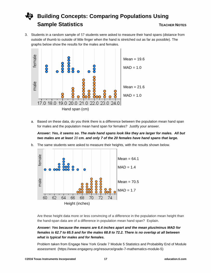
3. Students in a random sample of 57 students were asked to measure their hand spans (distance from

outside of thumb to outside of little finger when the hand is stretched out as far as possible). The

graphs below show the results for the males and females.

a. Based on these data, do you think there is a difference between the population mean hand span

for males and the population mean hand span for females? Justify your answer.

Answer: Yes, it seems so. The male hand spans look like they are larger for males. All but

two males are at least 20 cm. and only 7 of the 20 females have hand spans that large.

b. The same students were asked to measure their heights, with the results shown below.

Are these height data more or less convincing of a difference in the population mean height than

the hand-span data are of a difference in population mean hand span? Explain.

Answer: Yes because the means are 6.4 inches apart and the mean plus/minus MAD for

females is 62.7 to 65.5 and for the males 68.8 to 72.2. There is no overlap at all between

what is typical for males and for females.

Problem taken from Engage New York Grade 7 Module 5 Statistics and Probability End of Module

assessment (https://www.engageny.org/resource/grade-7-mathematics-module-5)

Mean = 64.1

MAD = 1.4

Mean = 70.5

MAD = 1.7

Height (inches)

Mean = 19.6

MAD = 1.0

Mean = 21.6

MAD = 1.0

Hand span (cm)




Student Activity Solutions

In these activities you will make conjectures about differences between two populations and compare two

populations and make informal inferences about the difference between them. After completing the

activities, discuss and/or present your findings to the rest of the class.

Activity 1 [Page 2.2 and 2.3]

1. Which of the following results is unlikely to occur by chance when sampling from this district? Give an

example from the TNS activity to support your reasoning.




Sample 4 Boys’ mean minus girls’ mean was 0.5.

Answers may vary slightly due to random generation of samples. The simulated sampling distribution

should indicate that 0 and 0.5 are very unlikely to happen when sampling from this district. A

difference of 4 did not occur often, while a difference of 3 was common.

2. Go to page 2.3. These samples come from surveys of students in another district.

a. Look at the distributions, then go to page 2.2 and Reset. How do the distributions on page 2.2

compare to the distributions on page 2.2?

Answer: The distributions are the same.

b. Go back to page 2.3 and generate 10 samples. Looking at the last two samples, would you say

there was a difference between the number of hours per week boys and girls typically spend doing

homework?

Answers may vary. In one case, the 10th sample had a difference in means of 0.4 which meant the

boys spent, on average, 0.4 hours more on homework than the girls. However, all of the boys

times were greater than the minimum girl time and less that the maximum girl time. This does not

indicate a difference in average time spent on homework for boys and girls in this district.

c. Did any simulation ever produce results where, on average, boys did more homework than the

girls? Explain your reasoning.

Answers may vary. If boys did more homework on average, then the difference in the sample

means would be positive. About half of the differences in the means were positive.

d. Generate at least 100 samples. Describe the simulated distribution of sample differences. What

would you conclude about the number of hours spent per week on homework by boys and by girls

in this district?

Answer: The simulated distribution is mound shaped and relatively symmetric, with a center

around 0 hours. The range goes from about 1.5 to 1.5 hours. This simulated sampling

distribution suggests that boys and girls in this district seem to spend about the same amount of

time doing homework.




3. Which of the outcomes below would be least likely to occur by chance when sampling from this

district? Give an example from the TNS activity to support your reasoning.




Answers will vary. The simulated sampling distribution should indicate that only a difference of 3 was

unusual. All of the other differences were common in the distributions.

4. Suppose you drew random samples of 20 boys and 20 girls from another district and asked them

about the number of hours they spent on homework each week.

a. Interpret the following statement: Mean girls – mean boys = 2.5

Answer: The girls typically spent 2.5 more hours per week doing homework than boys.

b. Write an equation showing that a sample of boys spent more time, on average, doing homework

than girls.

Answers will vary: Mean boys – mean girls = 2.

c. Marcus said all you needed to know was the means of a random sample from two populations and

a small difference between the two means, like 1.5, would be evidence that the populations are

different. What would you say to Marcus? Give an example to explain your answer.

Answers will vary. Students should recognize that knowing the difference in means without

knowing how the distributions vary is not enough information to see if there is really a difference. A

good example is the district shown on page 2.3. A difference of 1.5 hours occurred often in the

simulation, but because the distributions of times for the boys and girls overlapped so much,

sometimes the boys were higher by 1.5 hours and sometimes the girls were higher by 1.5 hours.

Even though there could be a difference between the sample means, if the distributions overlap a

lot, it is impossible to tell if there is actually a difference.




Activity 2 [Pages 2.2 and 2.3]

1. Work with several partners to investigate comparing differences in means when the sample sizes for

each sample both increase. Using sample sizes of 10, 40, 60 and 100, generate simulated sampling

distributions of the sample means for pages 2.2 and 2.3.

a. Fill in the table for the spread of the means in each distribution.

Sample

size

Page 2.2- sampling

distribution of the

difference in means

Length of

interval: |max-

min|

Page 2.3- spread

of difference in

means

Length of

interval: |max-

min|

10 –4.7 to –0.7 4 –2 to 2 4

40 –3.5 to –1.0 2.5 –1.2 to 1.2 2.4

80 –3 to –1.5 1.5 –0.8 to 0.8 1.6

100 –2.8 to –1.5 1.3 –0.8 to 0.5 1.3

b. Compare your distributions with those of your partners. What conjecture would you make about

how sample size affects the distributions of the differences in sample means for the number of

hours of homework for boys and girls?

Answer: As the sample size increases, the variability in the differences in the sample means of the

hours per week that boys and girls do homework decreases. It makes it much easier to see if

there really is a difference.

comparing populations using sample statistics

Documents